06-Garagash Large Toughness

Engineering Fracture Mechanics 73 (2006) 456–481

www.elsevier.com/locate/engfracmech

Plane-strain propagation of a fluid-driven fracture duringinjection and shut-in: Asymptotics of large toughness

Dmitry I. Garagash *

Department of Civil and Environmental Engineering, Clarkson University, 230 Rowley Laboratories, 8 Clarkson Ave.,

Potsdam, NY 13699-5710, USA

Received 1 September 2004; received in revised form 14 June 2005; accepted 6 July 2005Available online 2 November 2005

Abstract

This paper considers the problem of plane-strain fluid-driven fracture propagating in an impermeable elastic mediumunder condition of large toughness or, equivalently, of low fracturing fluid viscosity. We construct an explicit solution for afracture propagating in the toughness-dominated regime when the energy dissipated in the viscous fluid flow inside thefracture is negligibly small compared to the energy expended in fracturing the solid medium. The next order correctionsin viscosity to this limiting solution are then derived, allowing the range of problem parameters corresponding to thetoughness-dominated regime to be established. The first-order small viscosity (large toughness) solution is shown to pro-vide an excellent approximation of the solution for the crack length in the wide range of the viscosity parameter. Further-more, this solution, when combined with the first-order small-toughness solution of Garagash and Detournay [Journal ofApplied Mechanics, 2005], provides a simple analytical approximation of the crack length solution in practically the entirerange of viscosity (toughness). It is also shown that the established method of asymptotic expansion in small parameter isequally applicable to study other small effects (e.g., fluid inertia) on the otherwise toughness-dominated solution. A solu-tion for the fracture evolution during shut-in (i.e., after fluid injection rate is suddenly stopped) is also obtained. This solu-tion, which corresponds to a slowing fracture evolving towards the toughness-dominated steady state, draws attention tothe possibility of substantial fracture growth after fluid injection is ceased especially under conditions when the fracturepropagation during injection phase is dominated by viscous dissipation. 2005 Elsevier Ltd. All rights reserved.

Keywords: Hydraulic fracture; Toughness; Inertia; Asymptotic solutions; Scaling

1. Introduction

The problem of a fluid-driven fracture in rock arises in various applications ranging from hydraulic frac-turing treatment used in the oil industry to stimulate oil production from underground reservoirs [1] to theformation of intrusive dykes in the earth crust and magma transport in the lithosphere [2]. Other applications

0013-7944/$ - see front matter 2005 Elsevier Ltd. All rights reserved.

doi:10.1016/j.engfracmech.2005.07.012

* Tel.: +1 315 268 6501; fax: +1 315 268 7985.E-mail address: [email protected]

mailto:[email protected]

D.I. Garagash / Engineering Fracture Mechanics 73 (2006) 456–481 457

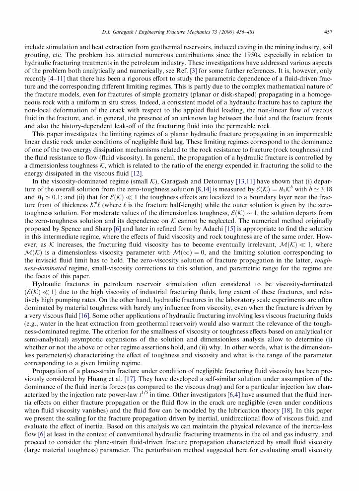
include stimulation and heat extraction from geothermal reservoirs, induced caving in the mining industry, soilgrouting, etc. The problem has attracted numerous contributions since the 1950s, especially in relation tohydraulic fracturing treatments in the petroleum industry. These investigations have addressed various aspectsof the problem both analytically and numerically, see Ref. [3] for some further references. It is, however, onlyrecently [4–11] that there has been a rigorous effort to study the parametric dependence of a fluid-driven frac-ture and the corresponding different limiting regimes. This is partly due to the complex mathematical nature ofthe fracture models, even for fractures of simple geometry (planar or disk-shaped) propagating in a homoge-neous rock with a uniform in situ stress. Indeed, a consistent model of a hydraulic fracture has to capture thenon-local deformation of the crack with respect to the applied fluid loading, the non-linear flow of viscousfluid in the fracture, and, in general, the presence of an unknown lag between the fluid and the fracture frontsand also the history-dependent leak-off of the fracturing fluid into the permeable rock.

This paper investigates the limiting regimes of a planar hydraulic fracture propagating in an impermeablelinear elastic rock under conditions of negligible fluid lag. These limiting regimes correspond to the dominanceof one of the two energy dissipation mechanisms related to the rock resistance to fracture (rock toughness) andthe fluid resistance to flow (fluid viscosity). In general, the propagation of a hydraulic fracture is controlled bya dimensionless toughness K, which is related to the ratio of the energy expended in fracturing the solid to theenergy dissipated in the viscous fluid [12].

In the viscosity-dominated regime (small K), Garagash and Detournay [13,11] have shown that (i) depar-ture of the overall solution from the zero-toughness solution [8,14] is measured by EðKÞ ¼ B1Kb with b ’ 3.18and B1 ’ 0.1; and (ii) that for EðKÞ 1 the toughness effects are localized to a boundary layer near the frac-ture front of thickness K6‘ (where ‘ is the fracture half-length) while the outer solution is given by the zero-toughness solution. For moderate values of the dimensionless toughness, EðKÞ 1, the solution departs fromthe zero-toughness solution and its dependence on K cannot be neglected. The numerical method originallyproposed by Spence and Sharp [6] and later in refined form by Adachi [15] is appropriate to find the solutionin this intermediate regime, where the effects of fluid viscosity and rock toughness are of the same order. How-ever, as K increases, the fracturing fluid viscosity has to become eventually irrelevant, MðKÞ 1, whereMðKÞ is a dimensionless viscosity parameter with Mð1Þ ¼ 0, and the limiting solution corresponding tothe inviscid fluid limit has to hold. The zero-viscosity solution of fracture propagation in the latter, tough-ness-dominated regime, small-viscosity corrections to this solution, and parametric range for the regime arethe focus of this paper.

Hydraulic fractures in petroleum reservoir stimulation often considered to be viscosity-dominatedðEðKÞ 1Þ due to the high viscosity of industrial fracturing fluids, long extent of these fractures, and rela-tively high pumping rates. On the other hand, hydraulic fractures in the laboratory scale experiments are oftendominated by material toughness with barely any influence from viscosity, even when the fracture is driven bya very viscous fluid [16]. Some other applications of hydraulic fracturing involving less viscous fracturing fluids(e.g., water in the heat extraction from geothermal reservoir) would also warrant the relevance of the tough-ness-dominated regime. The criterion for the smallness of viscosity or toughness effects based on analytical (orsemi-analytical) asymptotic expansions of the solution and dimensionless analysis allow to determine (i)whether or not the above or other regime assertions hold, and (ii) why. In other words, what is the dimension-less parameter(s) characterizing the effect of toughness and viscosity and what is the range of the parametercorresponding to a given limiting regime.

Propagation of a plane-strain fracture under condition of negligible fracturing fluid viscosity has been pre-viously considered by Huang et al. [17]. They have developed a self-similar solution under assumption of thedominance of the fluid inertia forces (as compared to the viscous drag) and for a particular injection law char-acterized by the injection rate power-law t1/5 in time. Other investigators [6,4] have assumed that the fluid iner-tia effects on either fracture propagation or the fluid flow in the crack are negligible (even under conditionswhen fluid viscosity vanishes) and the fluid flow can be modeled by the lubrication theory [18]. In this paperwe present the scaling for the fracture propagation driven by inertial, unidirectional flow of viscous fluid, andevaluate the effect of inertia. Based on this analysis we can maintain the physical relevance of the inertia-lessflow [6] at least in the context of conventional hydraulic fracturing treatments in the oil and gas industry, andproceed to consider the plane-strain fluid-driven fracture propagation characterized by small fluid viscosity(large material toughness) parameter. The perturbation method suggested here for evaluating small viscosity

458 D.I. Garagash / Engineering Fracture Mechanics 73 (2006) 456–481

effects on the otherwise toughness-dominated solution of a plane-strain hydraulic fracture is equally applicableto either other fracture geometries and/or to evaluate other small effects (such as fluid inertia) on the solution.

The paper is organized as follows. Firstly, we summarize the model describing a plane-strain fluid-drivenfracture and discuss the scaling of the sought solution for a general fluid injection law, the relevance of theinertia-less assumption, and the asymptotic zero-viscosity solution of a fracture propagating in the tough-ness-dominated regime. The next-order small-viscosity (large-toughness) solution is then obtained for twoinjection laws, namely, a constant injection rate and the shut-in (when injection rate is abruptly reduced tozero and the injected volume remaining constant thereafter), via an asymptotic series expansion in smalldimensionless viscosity, MðKÞ ¼ K4. (The utility of the series expansion method to evaluate small effectson the zero-viscosity solution other than that of the viscosity is demonstrated in Appendix C for the caseof small fluid inertia.) We conclude with the discussion of the parametric dependence of a fluid-driven fracturein view of the two limiting propagation regimes.

2. Problem formulation

Consider propagation of a finite two-dimensional fracture of half length ‘(t) in an impermeable linear elas-tic medium characterized by Youngs modulus E, Poissons ratio m, and toughness KIc. An incompressible fluidof viscosity l is injected at the center of the fracture at a rate Q(t), see Fig. 1, and the volume of injected fluid isgiven at any time t, V ðtÞ ¼

R t0Qdt. The crack is loaded by the internal fluid pressure pf(x, t) and by the far-field

confining stress r0. The fracture is assumed to be in mobile equilibrium at all times and its propagation isquasi-static. We will search for the solution of the fluid-driven fracture problem: the net pressure in the frac-ture p = pf(x, t) r0, the crack opening w(x, t), and the fracture half-length ‘(t), where x is the position alongthe crack and t is the time.

Main assumptions underlining the considered model of plane-strain fracture propagation are summarizedas follows:

• The fracture is fully fluid-filled at all times, i.e., there is no lag between the fracture and fluid front. Thisassumption is particularly relevant at or near the toughness-dominated propagation regime, when the frac-ture tip is ‘‘blunt’’ and the lag is an exponentially small function of toughness [9].

• Fracture propagation is described in the framework of linear elastic fracture mechanics (LEFM), charac-terized by the stress singularity at the fracture tip and the propagation criterion in mobile equilibriumrequiring the stress intensity factor to be equal to the material toughness KIc [19]. The LEFM assumptionrequires negligible inelastic deformations away form the fracture front and the smallness of the process zonenear the fracture front (wherein the inelasticity is assumed to be localized). The process zone at the fracturefront bears some similarity with the fluid lag behind the fracture front, as both regularize otherwise singularfields of stress and fluid pressure, respectively. The effect of the process zone on fracture propagation cangenerally be neglected (or represented via the effective fracture toughness [20]) when its dimension is smallcompared to the fracture extent and/or under the condition of large confining stress.

Fig. 1. Sketch of a plane-strain fluid-driven fracture.


• The flow of incompressible fluid in the fracture is unidirectional and laminar. These assumptions are jus-tifiable given the smallness of the crack opening compared to the crack length and small opening gradient[6], and low Reynolds number of the flow [4].

• No fluid exchange between the fracture and the surrounding solid is taking place.

Under above assumptions, the governing equations are formulated over the half of the crack, 0 6 x 6 ‘, onthe account of the problem symmetry. The formulation makes use of the following effective materialparameters:

E0 ¼ E1 m2

; l0 ¼ 12l; K 0 ¼ 42

p

1=2

KIc; ð1Þ

with the meaning of plane-strain elastic modulus, effective viscosity and toughness, respectively.The fluid flow in the fracture is governed by continuity of mass and momentum. An integral form of the

local continuity equation and the global fluid balance, stating that the injected fluid volume V(t) is equal tothe fracture volume, are given by

o

ot

Z ‘

xwdx ¼ wv;

Z ‘

0

wdx ¼ 1

2V ðtÞ; ð2Þ

where v(x, t) is the fluid mean velocity (in the cross-section normal to the flow) and wv is the fluid flow rate perunit (out-of-plane) width of the crack. In writing Eq. (2)a, the fluid velocity at the fracture tip, v(x = ‘) hasbeen taken equal to the tip velocity d‘/dt, following the zero fluid lag assumption. The momentum balanceequation for unidirectional laminar flow at small or very large values of Reynolds number is [21,4]

ovot

þ 1

2

ov2

ox¼ 1

qopox

þ l0vw2

; ð3Þ

where l 0v/w2 is the Poiseuille expression for the viscous shear stress in the laminar channel flow. The lubrica-tion flow approximation [18]

v ¼ w2

l0opox

ð4Þ

results from Eq. (3) when inertia terms (the left hand side of Eq. (3)) are neglected. Nilson [4,5] and Spence andSharp [6] argue for the lubrication approximation [Eq. (4)], whereas Huang et al. [17] consider inertial formu-lation [Eq. (3)] and neglect the viscous shear stress l 0v/w2. In the next section we analyze the scaling of theproblem and formulate the parametric regimes where one or the other assumption can be used.

The solid deformation and the fracture propagation criterion are prescribed by equations of linear elasticfracture mechanics. The crack opening w is related to the net pressure p by an integral equation [22],

wðx; tÞ ¼ 4

pE0

Z ‘

0

Gx‘;x0

‘

pðx0; tÞdx0; Gðn; n0Þ ¼ ln

ffiffiffiffiffiffiffiffiffiffiffiffiffi1 n2

pþ

ffiffiffiffiffiffiffiffiffiffiffiffiffiffi1 n02

pffiffiffiffiffiffiffiffiffiffiffiffiffi1 n2

p


p

. ð5Þ

The criterion of continuous quasi-static propagation of a fracture in mobile equilibrium, KI = KIc, is expressedas the tip asymptote of the crack opening [19]

w ¼ K 0

E0 ð‘ xÞ1=2 ‘ x ‘. ð6Þ

Eqs. (2), (3) or (4), and (5), (6) fully define the fracture length ‘(t), fluid velocity v(x, t), the opening w(x, t), andthe net pressure p(x, t) as functions of the parameter set [Eq. (1)], the fluid density q, and the injection law V(t).

3. Scaling

A particular insight into the different regimes of hydraulic fracture propagation and nature of correspond-ing solutions (e.g., self-similarity) can be gained from scaling considerations [4,6,23,9,24]. Following


Detournay [24], let us introduce the scaled coordinate n = x/‘(t) 2 [0, 1] and the following dimensionlessquantities: the opening X, the net pressure P, the crack half-length c, and the fluid velocity # as

wðx; tÞ ¼ eðtÞLðtÞXðn; tÞ; pðx; tÞ ¼ eðtÞE0Pðn; tÞ; ð7Þ‘ðtÞ ¼ LðtÞcðtÞ; vðx; tÞ ¼ t1LðtÞ#ðn; tÞ; ð8Þ

where L(t) is the crack lengthscale which is to be defined further for relevant fracture propagation regimes, and

eðtÞ ¼ L2ðtÞV ðtÞ ð9Þ
is a small dimensionless parameter with the meaning of a characteristic crack aspect ratio. Using the alterna-tive scaling for the opening and the velocity
Xðn; tÞ ¼ Xðn; tÞ=cðtÞ; #ðn; tÞ ¼ #ðn; tÞ=cðtÞ;
and scaling Eqs. (7)–(9), governing Eqs. (2) and (3), (5) and (6) can be written as follows:
• fluid mass:

t _VV

Z 1

nXdnþ t _L

LnXþWT ¼ X #;

Z 1

0

Xdn ¼ 1

2c2; ð10Þ

• fluid momentum:

Gqc2 #

t _LL

1 n#

o #

on

1þ o #

onþ UT

þ Gm

#

X2¼ oP

on; ð11Þ

• LEFM:

Xðn; tÞ ¼ L1fPgðn; tÞ; limn!1

ð1 nÞ1=2X ¼ Gkc1=2. ð12Þ

The overdot in above equations corresponds to the time derivative, o/ot, and elasticity operator L1 in Eq. (12)is defined by

L1fPgðn; tÞ ¼ 4

p

Z 1

0

Gðn; n0ÞPðn0; tÞdn0. ð13Þ

with the kernel G(n, n 0) given by Eq. (5)b. The terms WT and UT are time-transient parts in the continuity Eq.(10) and momentum Eq. (11), respectively,

WT ¼ tZ 1

n

_Xþ _cc

X noXon

dn; UT ¼ t _c

c1 n

#

o #

on

þ t _#

#. ð14Þ

Three dimensionless groups Gk, Gm, and Gq appearing in Eqs. (10)–(12) are defined as

Gk ¼K 0

E0L3=2

V; Gm ¼ l0

E0L6

tV 3; Gq ¼

qE0

L4

t2Vð15Þ

and quantify the relative effects of solid toughness, fluid viscosity, and fluid inertia, respectively. Formally, analgebraic constraint of the form Ga

kGbmG

cq ¼ 1 can be applied to these groups to fix the fracture lengthscale L in

Eqs. (7)–(9). Assuming injection power law of time, V ta, the fracture lengthscale L and the final form of thedimensionless groups resulting from the above constraint are respective power laws of time. Consequently,t _V =V and t _L=L in continuity Eq. (10)a and momentum Eq. (11) are the corresponding constant exponents,and the time derivative operator to(Æ)/ot in Eqs. (10), (11) and (14) can be replaced by

to

ot¼ t _Gk

Gk

!Gk

o

oGkþ t _Gm

Gm

!Gm

o

oGmþ t _Gq

Gq

!Gq

o

oGq; ð16Þ

where coefficients in the brackets are also constant exponents in the time power laws for Gk, Gm, and Gq, respec-tively. Consequently, the time dependence of the normalized solution of Eqs. (10)–(12) can be replaced by thatof dimensionless groups, resulting, e.g., for the opening X ¼ Xðn;Gk;Gm;GqÞ.


The three different physically motivated scalings [Eqs. (7)–(9)] (corresponding to the three different defini-tions of fracture lengthscale L) of the governing Eqs. (10)–(12) result from setting one of the three dimension-less groups [Eq. (15)] to unity. The lengthscale L, and the expressions of the dimensionless groups in thesethree scalings, identified as the toughness- ðGk ¼ 1Þ, the viscosity- ðGm ¼ 1Þ, and the inertia- ðGq ¼ 1Þ scalings,are presented in Table 1. The remaining two (non-unity) dimensionless groups in each scaling then define theparameters governing the solution of Eqs. (10)–(12). These parameters can have the meaning of either non-dimensionalized toughness (Ks), or viscosity (Ms), or inertia effects (Rs), see Table 1. The toughness- andthe viscosity scalings are naturally related to the asymptotic cases where dissipation in the solid due to frac-turing prevails over the dissipation in the viscous fluid (viscosity is irrelevant, Gm ¼ Mk ¼ 0) and vice a versa(toughness is irrelevant, Gk ¼ Km ¼ 0), respectively [24]. Corresponding number Gq (Rk or Rm) quantifies theeffect of inertia in these two scalings. The inertia-scaling can be naturally related to the asymptotic case whereinertia prevails over the viscous shear stresses (viscosity is irrelevant, Gm ¼ Mq ¼ 0). Parameter Gk ¼ Kq in thelatter case quantifies the effect of toughness in the inertia-dominated solution.

Solution of the governing Eqs. (10)–(12) in either one of the three scalings in Table 1 depends on twoparameters only (with the remaining dimensionless group equal to unity). Governing parameters in the threescalings are interrelated as follows:

TableQuant

Scaling

(k)

(m)

(q)

Mk ¼ K4m ; Rk ¼ M2=3

k Rm; Mq ¼ MkK4q ð17Þ

while the relations between dimensionless field variables X, P, #, and c in different scalings can be readilyestablished from scaling Eqs. (7)–(9) and the following relations between the three lengthscales Lk,m,q:

Lm

Lk¼ K2=3

m ;Lq

Lk¼ K2=3

q . ð18Þ

Examination of the toughness and the viscosity scalings shows that in the case of injection with a constant rate

Q0 (fracture volume is V = Q0t), the viscosity Mk and toughness Km parameters are constants while the cor-responding inertia parameters are negative power law of time ðRk;m t1=3Þ. Consequently, inertia effects maybe important at early stages of fracture propagation, but vanish with time. The corresponding large-timezero-inertia ðRk;m ¼ 0Þ asymptotic solution is self-similar, as originally observed by Spence and Sharp [6], sincethe remaining parameter Mk or Km is time-independent (the transient part of the fluid flux in fluid continuityEq. (10) is zero, WT = 0). This solution is characterized by the fracture length varying as t2/3. On the otherhand, early-time zero-toughness inertia-dominated asymptotic solution in inertia-scaling, Kq ¼ Mq ¼ 0, isalso self-similar, with the fracture length varying as t3/4.

Huang et al. [17] have considered a particular case of increasing injection rate, _V t1=5, which in the inertiascaling [Table 1] implies a constant value for the toughness parameter Kq and a positive time power law for theviscosity parameter, Mq t1=5. Their self-similar solution for inviscid fluid ðMq ¼ 0Þ characterized by thefracture length varying as t4/5, corresponds, therefore, to the early-time solution. In the case when injectionrate _V increases with time faster than t1/3, effects of both toughness and viscosity on the fracture propagationdecrease with time (see the inertia scaling in Table 1) as the fracture evolves towards the inertia-dominatedregime.

Examination of the toughness, the viscosity, and the inertia scalings during the shut-in (when the injectionrate is suddenly reduced to zero and the injected volume remaining constant thereafter), _V ¼ 0, shows that

1ities corresponding to toughness (k), viscosity (m) and inertia (q) scalings

L Gk Gm Gq

Lk ¼E0VK 0

2=3 1 Mk ¼l0VE0t

E0

K 0

4

Rk ¼qE05=3V 5=3

K 08=3t2

Lm ¼ E0V 3tl0

1=6

Km ¼ K 0

E0E0tl0V

1=4

1 Rm ¼ qV

l02=3E01=3t4=3

Lq ¼ E0Vt2

q

1=4

Kq ¼ K 0

E0E0t2

qV 5=3

3=8

Mq ¼ l0E01=2t2

q3=2V 3=21


Mk t1, Rk t2; Km t1=4, Rm t4=3; and Kq t3=4, Mq t2, respectively. Thus, the shut-in solutionevolves towards the zero-inertia toughness-dominated asymptotic limit ðMk ¼ Rk ¼ 0Þ, while the early-timeshut-in regime has to be determined by the corresponding regime at the end of the injection phase (prior tothe shut-in) given the continuity of the governing parameters between the injection and the shut-in.

Following the above discussion, the criterion for negligible fluid inertia effect on hydraulic fracture pro-pagation can be formulated as the smallness of appropriate inertia parameter

Rk ¼qE05=3V 5=3

K 08=3t2 1 when Mk ¼

l0VE0t

E0

K 0

4

K 1; ð19Þ

Rm ¼ qV

l02=3E01=3t4=3 1 when Mk J 1. ð20Þ

The duality of the above criterion reflects a simple observation that the inertia effects are quantified by twodifferent parameters (Rk vs. Rm) in the two extremities of fracture propagation dominated by the toughnessðMk 1Þ and the viscosity ðMk 1Þ, respectively. Let us consider a parameter set consistent with the appli-cation of hydraulic fracturing to the well-stimulation in petroleum industry: q = 103 kg/m3, l = 107 MPa s(100 cp), E 0 = 10 GPa, KIc = 1 MPa Æ m1/2 and a constant injection rate value Q0 = 104 m2 s1. For the aboveset at t = 1 min and at t = 1 h the fracture lengthscales are Lk Lm 7 m and Lk Lm 100 m, respectively,and the inertia parameters areRk Rm 105 andRk Rm 106, respectively. Clearly, the effect of inertiacan be neglected in this case. Furthermore, the dependence of inertia numbers on pumping time is weakðRk;m t1=3Þ and injection rates as high as Q0 0.1 m2 s1 would be required for a sizable inertia effectðRk;m 1Þ for the propagation time t > 1 min. Even though, out of the practical range in traditional hydraulicfracturing treatments, high values of the injection rate are conceivable over a short time period in an explosive-generated fracture.

The main focus of the following analysis is on the case where the fluid inertia can be neglected ðRk;m ¼ 0Þand the effect of the fluid viscosity on the fracture propagation is small compared to the effect of the materialtoughness (Mk 1 and Km 1). We acknowledge, however, that the perturbation method, which is devel-oped in the forthcoming Section 6.1 in order to study small viscosity effects in the inertia-less solution, isequally applicable to study other small effects, e.g., the effects of the fluid inertia (see Appendix C).

4. Equations in toughness scaling with no inertia

Unless stated otherwise, we assume the case of the inertia-less fluid flow in a fracture [Eqs. (19) and (20)],which results in the lubrication theory [Eq. (11) with Gq ¼ 0 or Eq. (4)]. Solution in the toughness scaling thendepends on a single parameter, the dimensionless viscosity Mk. Omitting hereafter the scaling index k forbrevity, solution in the toughness scaling

Fðn;MÞ ¼ fXðn;MÞ;Pðn;MÞ; #ðn;MÞ; cðMÞg ð21Þ
is governed by the reduced form of fluid mass and momentum Eqs. (10) and (11)
t _VV

Z 1

nXdnþ 2

3nX

þWT ¼ X

3

MoPon

;

Z 1

0

Xdn ¼ 1

2c2ð22Þ

and the unchanged LEFM Eq. (12)

Xðn;MÞ ¼ L1fPgðn;MÞ; limn!1

ð1 nÞ1=2X ¼ c1=2. ð23Þ

In the continuity Eq. (22)a, reduced Poiseuille momentum Eq. (11), # ¼ X2

MoPon , has been used, and elasticity

operator L1 in Eq. (23)a is defined by Eq. (13). The expression for the transient part WT [Eq. (14)] of the fluidflux is given by

WT ¼ t _MZ 1

n

oXoMþ 1

cdcdM X n

oXon

dn. ð24Þ


Consider a fluid injection law in the form

Q ¼ Q0½HðtÞ Hðt tÞ ð25Þ
(where H(Æ) is the Heavyside function) corresponding to a constant rate _V ¼ Q0 from t = 0 to a certain time t*,followed by the shut-in. The form of parameters in the toughness scaling [Table 1] and of the lubrication Eq.(22) can be further particularized for the two parts of the injection history [Eq. (25)] as follows.
During the injection phase at a constant rate Q0 (0 < t < t*), the crack lengthscale Lk and the dimensionlessviscosity M reduce to

Lk ¼E0Q0tK 0

2=3

; M ¼ l0Q0

E0E0

K 0

4

; 0 < t < t. ð26Þ

Since M is a constant, the transient term WT in Eq. (22)a vanishes and Eqs. (22) assume a self-similar form

MZ 1

nXdnþ 2

3nX

¼ X

3 dPdn

;

Z 1

0

Xdn ¼ 1

2c2. ð27Þ

This is the self-similarity originally discovered by Spence and Sharp [6].During the shut-in (t > t*), the injection volume remains constant, V(t) = V* = Q0t*, and the crack length-

scale Lk and the dimensionless viscosity M reduce to

Lk ¼E0V

K 0

2=3

; M ¼ l0V

E0tE0

K 0

4

¼ Mtt; t > t; ð28Þ

where M ¼ l0Q0E03=K 04 is the constant value of the dimensionless viscosity at t = t*, according to Eq. (26)b,

and V* = Q0t* is the constant value of the crack volume during the shut-in. Since the term multiplied by t _VV in

Eqs. (22) is zero for t > t*, Eqs. (22) with (24) become

t > t:Z 1

n

oX

oM1þ 1

cdc

dM1X n

oXon

dn ¼ X

3 oPon

;

Z 1

0

Xdn ¼ 1

2c2; ð29Þ

where M1 plays a role of dimensionless time [Eq. (28)b]. Note that, even though injection rate is discontin-uous at t* , the scaling lengthscale Lk is continuous, as well as the normalized solution for the opening X, thenet pressure P, and the crack half-length c.

The dimensionless viscosity M characterizes the relative importance of the fluid viscous properties l 0 andthe solid toughness K 0 for hydraulic fracture propagation. In this paper we focus on the ‘‘large toughness’’ (or,alternatively, ‘‘small viscosity’’) solution for a fluid-driven fracture. The large toughness solution is sought as aseries expansion in terms of the viscosity M, with the first term of the expansion, O(1), corresponding to thezero-viscosity solution ðM ¼ 0Þ and the subsequent terms (M1, M2, etc.) providing the next-order viscositycorrections. Under conditions when the viscosity correction is small, the fracture is said to propagate in thetoughness-dominated regime, which corresponds to the zero-viscosity solution.

5. Zero-viscosity solution

The zero-viscosity solution F 0ðnÞ ¼ Fðn; 0Þ is independent of the injection law. Eqs. (22) and (23) withM ¼ 0 yield

0 ¼ X3

0

dP0

dn; c2

0 ¼ 2

Z 1

0

X0 dg; ð30Þ

X0 ¼ L1fP0g; limn!1

ð1 nÞ1=2X0 ¼ c1=20 . ð31Þ

Solution of Eqs. (30) and (31) corresponds to uniform net pressure along the crack and the corresponding clas-sical elliptic crack opening

X0 ¼p1=3

2


q; P0 ¼

p1=3

8’ 0:1831; c0 ¼

2

p2=3’ 0:9324. ð32Þ


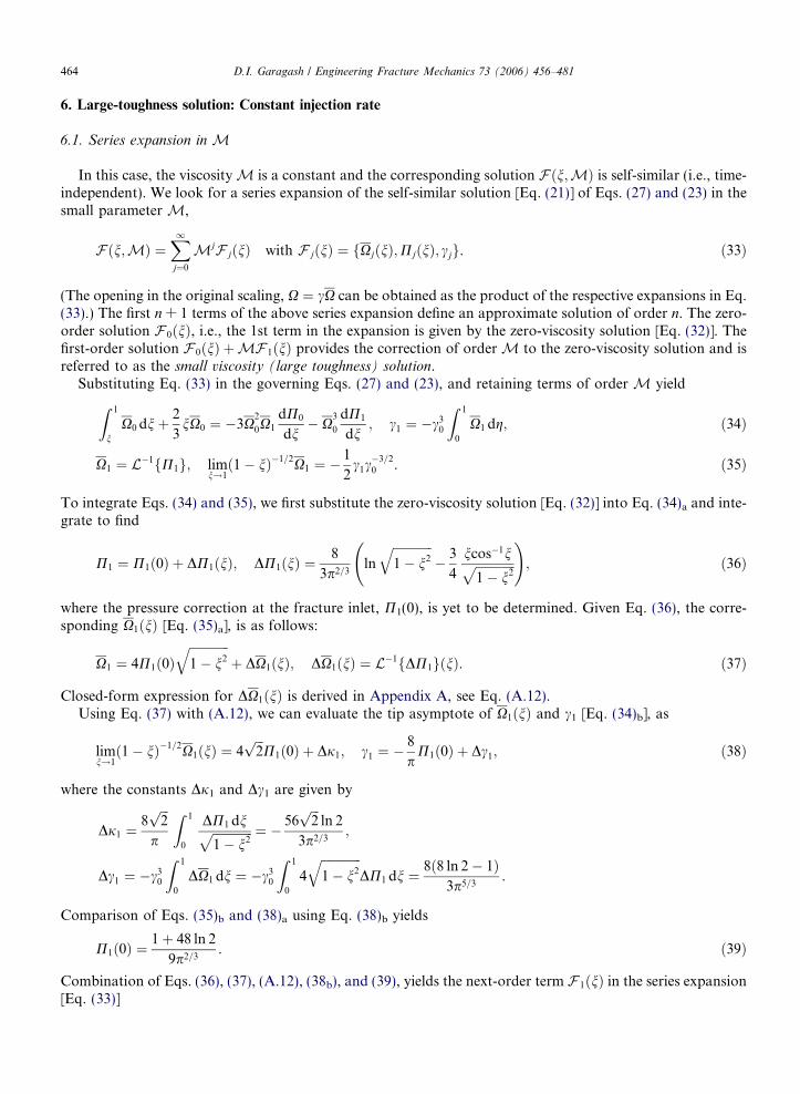
6. Large-toughness solution: Constant injection rate

6.1. Series expansion in M

In this case, the viscosity M is a constant and the corresponding solution Fðn;MÞ is self-similar (i.e., time-independent). We look for a series expansion of the self-similar solution [Eq. (21)] of Eqs. (27) and (23) in thesmall parameter M,

Fðn;MÞ ¼X1j¼0

MjF jðnÞ with F jðnÞ ¼ fXjðnÞ;PjðnÞ; cjg. ð33Þ

(The opening in the original scaling, X ¼ cX can be obtained as the product of the respective expansions in Eq.(33).) The first n + 1 terms of the above series expansion define an approximate solution of order n. The zero-order solution F 0ðnÞ, i.e., the 1st term in the expansion is given by the zero-viscosity solution [Eq. (32)]. Thefirst-order solution F 0ðnÞ þMF 1ðnÞ provides the correction of order M to the zero-viscosity solution and isreferred to as the small viscosity (large toughness) solution.

Substituting Eq. (33) in the governing Eqs. (27) and (23), and retaining terms of order M yield
Z 1
nX0 dnþ

2

3nX0 ¼ 3X

2

0X1

dP0

dn X

3

0

dP1

dn; c1 ¼ c30

Z 1

0

X1 dg; ð34Þ

X1 ¼ L1fP1g; limn!1

ð1 nÞ1=2X1 ¼ 1

2c1c

3=20 . ð35Þ

To integrate Eqs. (34) and (35), we first substitute the zero-viscosity solution [Eq. (32)] into Eq. (34)a and inte-grate to find

P1 ¼ P1ð0Þ þ DP1ðnÞ; DP1ðnÞ ¼8

3p2=3ln


q 3

4

ncos1nffiffiffiffiffiffiffiffiffiffiffiffiffi1 n2

p !

; ð36Þ

where the pressure correction at the fracture inlet, P1(0), is yet to be determined. Given Eq. (36), the corre-sponding X1ðnÞ [Eq. (35)a], is as follows:

X1 ¼ 4P1ð0Þffiffiffiffiffiffiffiffiffiffiffiffiffi1 n2

qþ DX1ðnÞ; DX1ðnÞ ¼ L1fDP1gðnÞ. ð37Þ

Closed-form expression for DX1ðnÞ is derived in Appendix A, see Eq. (A.12).Using Eq. (37) with (A.12), we can evaluate the tip asymptote of X1ðnÞ and c1 [Eq. (34)b], as

limn!1

ð1 nÞ1=2X1ðnÞ ¼ 4ffiffiffi2

pP1ð0Þ þ Dj1; c1 ¼ 8

pP1ð0Þ þ Dc1; ð38Þ

where the constants Dj1 and Dc1 are given by

Dj1 ¼8ffiffiffi2

p

p

Z 1

0

DP1 dnffiffiffiffiffiffiffiffiffiffiffiffiffi1 n2

p ¼ 56ffiffiffi2

pln 2

3p2=3;

Dc1 ¼ c30

Z 1

0

DX1 dn ¼ c30

Z 1

0

4


qDP1 dn ¼ 8ð8 ln 2 1Þ

3p5=3.

Comparison of Eqs. (35)b and (38)a using Eq. (38)b yields

P1ð0Þ ¼1þ 48 ln 2

9p2=3. ð39Þ

Combination of Eqs. (36), (37), (A.12), (38b), and (39), yields the next-order term F 1ðnÞ in the series expansion[Eq. (33)]

2

-2

-1

0

1

2

4

6

0 0.2 0.4 0.6 0.8 10

0 0.2 0.4 0.6 0.8 1

Ω

ξ ξ

Ω

Ω

ΠΠ

Π

1

0

1

0

(a) (b)

Fig. 2. (Constant injection rate, zero inertia) Zero- and first-order viscosity terms of normalized opening, (a), and net-pressure, (b), in thesmall viscosity solution.


X1 ¼8

3p2=32p 4nsin1n 5

6 ln 2


q 3

2ln

1þffiffiffiffiffiffiffiffiffiffiffiffiffi1 n2

p 1þ ffiffiffiffiffiffiffi1n2

p

1ffiffiffiffiffiffiffiffiffiffiffiffiffi1 n2

p 1 ffiffiffiffiffiffiffi1n2

p

2664

3775

0BB@

1CCA; ð40Þ

P1 ¼8

3p2=3

1

24þ ln 4


q 3

4

ncos1nffiffiffiffiffiffiffiffiffiffiffiffiffi1 n2

p !

; ð41Þ

c1 ¼ 32ð1þ 6 ln 2Þ9p5=3

’ 2:7220. ð42Þ

Profiles of opening and pressure for the zero-viscosity solution [Eq. (32)] and the first-order terms [Eqs. (40)–(42)] are shown in Fig. 2.

6.2. Discussion

Similarly to the first-order term above, we can work out terms in the expansion [Eq. (33)] to any givenorder, OðMjÞ, jP 2. These terms and their integrals have to be implemented numerically in view of theirincreasing complexity with increasing term-order. The results for the coefficients of the high-order expansionterms (up to OðM10Þ) for the crack half-length c, the net pressure P(0), and the opening Xð0Þ at the inlet aresummarized in Table 2.

The plot of the zero-order O(1), the first-order OðMÞ and the higher order OðM10Þ small viscosity solutionsfor the crack half-length c [dashed lines in Fig. 3] in comparison to the finite viscosity numerical solution [15](open circles) show that the small viscosity expansion diverges at M ¼ Oð0:01Þ. Using standard methods ofanalysis and improvement of diverging series [25], we can establish that the small viscosity series divergedue to a nearest (non-physical) singularity on the negative real axis of the parameter M, M ¼ Msi withMsi ’ 0:0333, of the form c const ðMþMsiÞ1=2, see Appendix B. This suggests an Euler transformation,or a reformulation of the small viscosity series in terms of the following small parameter

dðMÞ ¼ Mffiffiffiffiffiffiffiffiffiffiffiffiffiffiffiffiffiffiffiffiffiffiffiffiffi1þM=Msi

p . ð43Þ

This transformation eliminates the singularity and increases the radius of series convergence (improves the ser-ies). The series in terms of dðMÞ are obtained by the substitution of the inverse of Eq. (43), MðdÞ, into theviscosity expansion [Eq. (33)] and expanding the result into the Tailor series in d. Since dðMÞ is equal tothe first order to M, the improved first-order small viscosity solution is of particularly simple form,F 0ðnÞ þ dðMÞF 1ðnÞ.

The plot of the O(d) and the O(d10) solutions [solid lines in Fig. 3] show at least an order of magnitudeincrease of the radius of convergence of the small viscosity expansion. The eventual divergence of theimproved series may indicate the emergence of a new state of the solution influenced by the viscosity to an

Table 2Numerical values of coefficients of the OðMjÞ terms (j = 0,1, . . . ,10) in the expansion [Eq. (33)] of crack half-length c, net pressure P(0)and normalized opening Xð0Þ at the inlet

cj · 0.04j Pj(0) · 0.04j Xjð0Þ 0:04j

j = 0 +0.93239 +0.18307 +0.73229j = 1 0.10888 +0.07101 +0.30548j = 2 +0.05961 0.03171 0.07971j = 3 0.04528 +0.02359 +0.05544j = 4 +0.04003 0.02099 0.04726j = 5 0.03864 +0.02049 +0.04479j = 6 +0.03951 0.02120 0.04532j = 7 0.04206 +0.02282 +0.04792j = 8 +0.04613 0.02527 0.05234j = 9 0.05177 +0.02860 +0.05857j = 10 +0.05917 0.03294 0.06681

0.001 0.01 0.1 10.5

0.6

0.7

0.8

0.9

1.0

γ

Fig. 3. (Constant injection rate, zero inertia) Zero-viscosity O(1) solution and small viscosity solutions for the crack half-length: theoriginal series expansions [Eq. (33)] to OðMÞ and OðM10Þ (dashed lies) and the improved series expansions to O(d) and O(d10) (solid lines).Open circles show finite toughness (viscosity) numerical solution (after Adachi [15]).


extent which cannot be captured by corrections to the otherwise toughness-dominated state. This new statehas to be intimately related to the existence of an intermediate tip asymptote defined by viscous dissipation[11], and characterized by the opening varying as (1 n)2/3 at some (small) distance away from the tipn = 1, which cannot be correctly captured by the small-viscosity solution with the near tip opening behaviorof the form (1 n)1/2.

The improved first-order solution for the net pressure, P ¼ P0 þ dðMÞP1 and the opening in the originalscaling X ¼ ðc0 þ dðMÞc1ÞðX0 þ dðMÞX1Þ is shown in Fig. 4 for various values of the viscosity M ¼f0; 0:01; 0:03; 0:1g. The O(d) solution agrees well with the numerical solution [15] (shown by open circles) withsome departure observed at a higher viscosity value M ¼ 0:1. (Note that the O(d) approximation of the cracklength c [Fig. 3] is apparently more accurate than the O(d) approximation for the opening and the net pres-sure.) Since the first-order solution depends linearly on dðMÞ ¼ MþOðM2Þ, the increase in the viscosity Mfrom 0 to 0.1 entails a significant departure from the zero-viscosity limit (Fig. 4). On the other hand, the solu-tion converges rapidly towards the zero-viscosity limit with increasing toughness K ¼ M1=4 [Eq. (17)a].

Owing to the logarithmic tip singularity of the viscosity correction to the net pressure, dðMÞP1ðnÞ, the zero-viscosity approximation breaks down near the fracture tip. Indeed, the approximation error introduced by thezero-viscosity solution for the net pressure is OðdðMÞÞ away from the tip, 1 n = O(1), and O(1) or greater inthe near tip region defined by 1 n ¼ O exp 3p

32M1

. Consequently, the viscosity correction to the net

pressure has to be accounted for in the solution regardless of the smallness ofM in order to accurately capture

ξ

Ω

0.00.0 0.2 0.4 0.6 0.8 1.0

ξ0.0 0.2 0.4 0.6 0.8 1.0

0.2

0.4

0.6

0.8

Π

0.12

0.15

0.18

0.21

0.24

0.27

0.30

=0

=0.1

(a) (b)

0

0.01

0.03

0.1

Fig. 4. (Constant injection rate, zero inertia) Dimensionless opening X ¼ cX and net pressure P in the improved first-order smallviscosity solution for various values of M.


the near tip behavior. Note, however, that the extent of the latter near tip region, where the zero-viscosity pres-sure solution P0(n) is not an accurate approximation, is exponentially small.

The zero-viscosity solution governs fracture propagation in the toughness-dominated regime, whilst thesmall viscosity solution provides a viscosity correction to the latter solution, and, therefore, can be used toestimate the parametric range of the toughness-dominated regime. Indeed, the threshold value of viscosityM0 ’ 3:4 103 for the toughness-dominated regime ðM < M0Þ can be obtained by requiring a 1% maximumdeviation in the dimensionless fracture length from the zero-viscosity solution, i.e., M0 ¼ 0:01jc0=c1j ’0:0034. The corresponding threshold value of toughness K1 ¼ M1=4

0 for the toughness-dominated regimeðK > K1Þ is then estimated as K1 ’ 4:13.

6.2.1. Remark on small inertia effects on zero-viscosity solution

The perturbation method suggested in Section 6.1 to study the effect of small viscosity on the inertia-lesspropagation of a plane-strain fluid-driven fracture can be applied (i) to other one-dimensional fracture geom-etries (e.g., an edge crack or a radial crack) and/or (ii) to analyze other small effects in the fluid flow in a prop-agating fracture (e.g., inertia).

Indeed, in the case of a different one-dimensional fracture geometry, the method is directly applicable giventhe appropriate form of kernel G [Eq. (13)] in the elasticity integral operator L1fg, see Eqs. (31)a and (35)a;and, in the case of a radial fracture [10], the appropriate form of the toughness scaling and of the lubricationequations.1

On the other hand, the analysis using the method of Section 6.1 of the effect of small fluid inertia on thepropagation of a plane-strain fracture driven by inviscid fluid is given in Appendix C. The small inertia solu-tion is obtained in the toughness scaling in the form

1 Th

F ¼X1j¼0

ðRðtÞÞjF jðnÞ with F jðnÞ ¼ fXjðnÞ;PjðnÞ; cjg; ð44Þ

where F 0ðnÞ is the zero-viscosity, zero-inertia solution [Eq. (32)] and subsequent terms are the inertia correc-tions. The zero-order (zero-inertia) and the next-order small inertia solutions up to the OðR5Þ for the fracturedimensionless half-length cðRÞ are shown in Fig. 5.

The OðR5Þ small inertia solution for the dimensionless opening X and the net pressure P is shown in Fig. 6for various values of inertia parameter, R ¼ f0; 0:1; 0:2; 0:3; 0:4; 0:5g. It is interesting to point out that the netpressure increases in the direction of the flow from the injection point to the fracture tip. This result, alsoreported by Huang et al. [17] for a special case of increasing injection rate with time, can be attributed tothe Bernoullis effect for the flow of inviscid fluid with the decreasing velocity in the direction of the flow.For a flow of a viscous fluid with negligible inertia, the net pressure decreases in the direction of the flowdue to the viscous dissipation, see, e.g., Fig. 4(b). Conceivably, if effects of viscosity and inertia are compara-ble, the net pressure may develop a non-monotonic profile with the maximum in the interior of the crack.

e scaling and the lubrication equations for the case of an edge plane-strain crack are identical to that of a Griffiths crack.

γ

0.90

0.95

1.00

1.05

1.10

1.15

0.0 0.1 0.2 0.3 0.4 0.5 0.6

Fig. 5. (Constant injection rate, zero viscosity) Small inertia solutions [Eq. (33)] for crack half-length to OðRnÞ; c ¼Pn

j¼0Rjcj, withn = 0,1, . . . , 5.

ξ ξ

Ω

0.00.0 0.2 0.4 0.6 0.8 1.0 0.0 0.2 0.4 0.6 0.8 1.0

0.2

0.4

0.6

0.8

Π

0.00

0.05

0.10

0.15

0.20

0.25

=0.5

=0

(b)(a)

=0.5

=0

0.4

0.20.1

0.3

Fig. 6. (Constant injection rate, zero viscosity) The OðR5Þ small inertia solution for dimensionless opening X ¼ cX, (a), and net pressureP, (b), for various values of R.


Since the net pressure in the zero-viscosity solution has the minimum at the injection point, the crack maytend to develop a tear-drop shape for larger values of the inertia parameter R, as shown in Fig. 6(a).

7. Large-toughness solution: Shut-in

In this section we construct a solution for a fluid-driven fracture during the shut-in (t P t*) which followsthe injection phase at a constant rate Q0 (t < t*) described by the first-order large-toughness solution developedin Section 6.

7.1. Nature of the solution

Let us define a dimensionless time s starting with the shut-in instant, i.e., s(t*) = 0,

s ¼ 1

M 1

M¼ 1

M

tt 1

; ð45Þ

where MðtÞ ¼ Mt=t is the dimensionless viscosity during the shut-in (tP t*), see Eq. (28), and M is theconstant value of dimensionless viscosity prior to the shut-in (t 6 t*), see Eq. (26). In view of Eq. (45), it isconvenient to define the solution in terms of the shut-in time s (instead of M), as

F sðn; sÞ ¼ Fðn;MðsÞÞ. ð46Þ


Prior to the shut-in (s 6 0), the solution is given by the self-similar large-toughness solution in the constantinjection rate case [Eq. (33)], with M ¼ M 1,

F sðn; s 6 0Þ ¼ Fðn;MÞ ¼ F 0ðnÞ þMF 1ðnÞ þ ; ð47Þ

where the zero-viscosity solution F 0ðnÞ and the next-order viscosity correction F 1ðnÞ, are given by Eqs. (32)and (40)–(42), respectively. Eq. (47) then provides the initial condition for the shut-in solution F s ðn; s P 0Þ,which is governed by Eq. (29) with oðM1Þ ¼ os, (45), and (23). The self-similar zero-viscosity solution F 0ðnÞsatisfies the shut-in governing equations, but contradicts the initial condition at s = 0 [Eq. (47)], which differsfrom F 0ðnÞ by terms of order M. Consequently, the shut-in solution has to evolve from the initial viscosity-dependent state [Eq. (47)] towards the zero-viscosity large-time limit. This evolution of the solution effectivelycorresponds to a ‘‘time-removal’’ of the initial viscosity term MF 1ðnÞ in Eq. (47). Acknowledging the shut-intime scaling [Eq. (45)] and the large-toughness condition, M 1, evolution of the fracture to the toughness-dominated regime given by the zero-viscosity solution F 0ðnÞ will take place over a small-time interval,t t* t*, and can be viewed as a time boundary layer.

Based on the initial condition [Eq. (47)] and the smallness of M, we can present the shut-in solution in theform of a series expansion in M

F sðn; s P 0Þ ¼ F 0ðnÞ þMF 1sðn; sÞ þ with F 1sðn; 0Þ ¼ F 1ðnÞ. ð48Þ

The term F 1sðn; sÞ ¼ fX1sðn; sÞ;P1sðn; sÞ; c1sðsÞg is the time-dependent correction to the zero-viscosity solutionF 0ðnÞ. The former vanishes for large time s, F 1sðn; s ! 1Þ ¼ 0.

Substitution of the series expansion [Eq. (48)] with Eqs. (32) and (45) into Eqs. (29), and (23) while retainingterms of order M, allows us to obtain the governing equations for F 1sðn; sÞ as follows:

_c1scos1nþ 4

p

Z 1

n

_X1s dn ¼ 2ð1 n2Þ3=2 oP1s

on; c1s ¼ 8

p2

Z 1

0

X1s dn; ð49Þ

X1s ¼ L1fP1sg; limn!1

ð1 nÞ1=2X1s ¼ pc1s25=2

; ð50Þ

where the overdot corresponds to o/os.Let us introduce the following representation for the opening X1s, pressure P1s, and crack length c1s terms:

X1sðn; sÞ ¼ c1sðsÞWðn; sÞ;P1sðn; sÞ ¼ c1sðsÞPðn; sÞ;

c1sðsÞ ¼ c1 expZ s

0

AðsÞds;ð51Þ

where A ¼ _c1s=c1s < 0 corresponds to the rate of exponential decay of the next-order viscosity correction c1sfor the fracture length cs. In view of Eq. (51), and a new field variable defined as

U ¼ cos1nþ 4

p

Z 1

nW dn; ð52Þ

the fluid flow Eq. (49) are reduced to

_U ¼ 2ð1 n2Þ3=2 oPon

AU; Ujn¼0 ¼ 0; ð53Þ

while the LEFM Eq. (50) become

W ¼ L1fPg; limn!1

ð1 nÞ1=2W ¼ p

25=2. ð54Þ

Initial conditions for W and P follow from Eq. (48), with Eq. (51) in the form

Wðn; 0Þ ¼ X1ðnÞ=c1; Pðn; 0Þ ¼ P1ðnÞ=c1. ð55Þ


The governing Eqs. (52)–(54) in scaling [Eqs. (51)], suggest a self-similar (i.e., time-independent) large-timesolution when _U in Eqs. (53) vanishes and the exponent A(s) tends to a constant value A(1) < 0. This self-similar solution has the meaning of an intermediate large-time asymptote, corresponding to the time whenthe details of the imposed initial conditions [Eqs. (55)], become irrelevant. This large-time solution corre-sponds to an exponential decay of the opening X1s, pressure P1s, and crack length c1s terms in time with con-stant exponential rate A(1) < 0, see Eqs. (51).

7.2. Method of solution

According to Eq. (52), _Ujn¼1 ¼ 0 , and the asymptotic form of the lubrication Eq. (53)a near the tip can beintegrated in n to yield a pressure-term asymptote, Pðn; sÞ ¼ 1

4AðsÞ lnð1 nÞ, as n ! 1. The initial value

A(0) = 3p/(2(1 + 6ln2)) can then be obtained by evaluating the latter asymptote at s = 0 and applyingthe pressure-term initial condition [Eq. (55)b] with P1(n) and c1 given by Eqs. (41) and (42), respectively.Finally, the pressure-term asymptote can be expressed in terms of the initial data and the time varying param-eter A(s),

n ! 1: Pðn; sÞ ¼ AðsÞAð0Þ Pðn; 0Þ. ð56Þ

Based on the asymptotic, Eq. (56), and initial value, Eqs. (55), considerations, we can represent the solutionfor P and W as a sum of (logarithmically) singular and regular parts as follows:

P ¼ AðsÞAð0Þ Pðn; 0Þ þ dPðn; sÞ; W ¼ AðsÞ

Að0ÞWðn; 0Þ þ dWðn; sÞ. ð57Þ

Functions dPðn; sÞ and dWðn; sÞ are regular in n 2 [0,1] with initial condition following from Eq. (55):

dPðn; 0Þ ¼ dWðn; 0Þ ¼ 0. ð58Þ
Continuity Eq. (53)b and elasticity Eqs. (54) yield
AðsÞAð0Þ 1 ¼ 8

p2

Z 1

0

dW dn; ð59Þ

dW ¼ L1fdPg; limn!1

ð1 nÞ1=2dW ¼ p

25=2AðsÞAð0Þ 1

. ð60Þ

Summarizing, via the representation [Eq. (57)], the solution for the pressure P, opening W, and crack lengthc1s reduces to the solution for the regular parts of the pressure and opening terms, dPðn; sÞ and dWðn; sÞ,respectively, and the exponent A(s) given by Eqs. (52), (53), (59), (60) and initial condition [Eq. (58)]. Thelarge-time self-similar asymptote of the above solution is governed by the latter equations with _U ¼ 0 inthe lubrication Eq. (53)a and the time-dependent exponent A(s) replaced by its limit value A(1).

Solution of Eqs. (52), (53), (59), (60), and (58) is sought via the numerical method of lines (see Liskovets [26]for general discussion, and Nilson and Griffiths [27] and Garagash and Detournay [28] for applications of themethod to hydraulic fracture problems). This method approximates Eqs. (59) and (60) by a coupled system ofordinary differential equations (ODEs) governing the time evolution of the values of dPðn; sÞ at the fixedgrid points over the space interval representing the crack. Details of the numerical method are given inAppendix D.

7.3. Results and discussion

Calculations of the solution fdWðn; sÞ; dPðn; sÞ;AðsÞg of Eqs. (52), (53), (59), (60), and (58) have been car-ried out using 26 grid points equally spaced along the half-length of the crack that include the inlet and the tip.(Convergence of the numerical scheme has been evaluated by carrying out calculations with 11 grid pointswhich produced practically identical results.) The corresponding normalized next-order terms in opening,W ¼ X1s=c1s, and pressure, P ¼ P1s=c1s, [Eq. (57)], along the crack are shown in Fig. 7 for various times. This

-2

-3

-1

0

-3 -2 -1 1

10log τ0

-1.1

-1

-0.9

A

Fig. 8. (Shut-in, zero-inertia) Evolution of next-order crack length term c1s(s) and its exponential decay rate A ¼ _c1s=c1s.

0 0.2 0.4 0.6 0.8 1

ξ

-2

-1.5

-1

-0.5

0

-1

-0.5

0

0.5

1

Fig. 7. (Shut-in, zero-inertia) Distribution of pressure P ¼ P1s=c1s and opening W ¼ X1s=c1s renormalized first-order terms in the shut-insolution expansion [Eq. (48)] along the crack for discrete time-set s ¼ 1

Mtt 1

¼ f0; 0:01; 0:05; 0:1;1g (time s = 0 corresponds to the

shut-in instant t = t*).


figure shows that overall variation of W and P with time s is marginal, and it is mainly driven by the stepchange of the gradient of the pressure term P at the inlet, n = 0, from the finite value corresponding to theinitial conditions (constant non-zero injection rate) to zero value instantaneously upon the shut-in. Conse-quently, the evolution of the next-order opening X1s ¼ c1sW , and pressure P1s ¼ c1sP terms in the shut-insolution expansion [Eq. (48)] is largely defined by the time evolution of the next-order term in the fracturelength, c1s.

Evolution of the length c1s and of its exponential rate A ¼ _c1s=c1s with time s is shown in Fig. 8 in a semi-logarithmic scale. The next-order crack length term c1s evolves from the initial value c1 [Eq. (42)] to zero atlarge time, when the shut-in solution approaches its large-time zero-viscosity limit. The rate A of exponentialdecay of c1s saturates at the large-time value A(1) ’ 1.1 for s J s1 = 0.33,2 see Fig. 8. Consequently, fors J s1, the next-order viscosity correction F 1sðn; sÞ in the shut-in solution [Eq. (48)] is given by the interme-diate large-time asymptote

2 Th

X1s ’ c1sðsÞWðn;1Þ; P1s ’ c1sðsÞPðn;1Þ; c1s ’ c1sðs1ÞeAð1Þðss1Þ; ð61Þ

is time threshold corresponds to the 0.1% difference between the solution A(s) and the asymptote A(1).

Ω

ξξ

τ Πτ

τ = 0 τ = 0τ = ∞

τ = ∞

0.2

0.4

0.6

0.8

0.17

0.15

0.19

0.21

0 0.2 0.4 0.6 0.8 10

0 0.2 0.4 0.6 0.8 1(b)(a)

Fig. 9. (Shut-in, zero-inertia) Dimensionless opening Xs ¼ csXs, (a), and net pressure Ps, (b), along the crack at various timess = 0,0.01,0.1,0.5,1,2.5,1 and initial value M ¼ 0:01 of the viscosity parameter.


where c1sðs1Þ ¼ c1 expR s10 AðsÞds ’ 1:923. Interestingly, the intermediate large-time asymptote for c1s [Eq.

(61)c] provides an excellent approximation for the whole shut-in time range, see dashed curve in Fig. 8.Fig. 9 shows the distribution of the dimensionless opening Xs and the net pressure Ps along the fracture

length for M ¼ 0:01 at various times. The shut-in solution evolves from the initial state (s = 0) given bythe small viscosity-solution with M ¼ 0:01 for the constant injection rate case towards the toughness-domi-nated large-time limit with M ¼ 0 [Fig. 4]. The solution is effectively given (within 1% accuracy) by thelarge-time toughness-dominated limit for s J 3.08 (as inferred from the considerations for the crack length[Eq. (61)c]), or, in physical time, t t J 3:08Mt. Evolution of the normalized crack lengthcs ¼ c0 þMc1sðsÞ during the shut-in can be trivially inferred from that of c1s(s), see Fig. 7(b).

Let us consider the evolution of fracture length in more detail. For an inviscid fluid, M ¼ 0, the normal-ized crack length is given by the zero-viscosity solution, cs = c0. Since the lengthscale of the fractureLk = (E 0V*/K

0)2/3 is constant during the shut-in [Eq. (28)a] (recall that Lk t2/3 [Eq. (26)a] during the constantinjection rate stage, t < t*), the fracture length remains unchanged during the shut-in, ‘ = Lkc0. For small butnon-zero dimensionless viscosity M, the dimensionless fracture length at the shut-in instant is given bycs ðs ¼ 0Þ ¼ c0 þMc1s ðs ¼ 0Þ, with c1s (s = 0) = c1 ’ 2.72 [Eq. (42)]. Thus, time removal of the initialviscosity length correction during the shut-in corresponds to further growth of the fracture byDcs ¼ Mc1 > 0. The dimensionless time interval during the shut-in, sstop, required for fracture dimension-less length cs to grow within 1% of its terminal length c0, can be estimated from the intermediate large-timeasymptote [Eq. (61)] as sstop ¼ 5:17þ 0:91 lnM. For example for M ¼ 0:01, sstop ’ 1 and the correspondingphysical time interval Dtstop is given by Dtstop=t ¼ Msstop ’ 0:01. The corresponding fracture length growthduring the shut-in as a fraction of its length ‘* at the end of the injection phase (t = t*) is given byD‘=‘ ’ Mc1=c0 ’ 2:9M, or 2.9% for M ¼ 0:01. Similarly, the terminal net pressure drop at the fractureinlet during the shut-in is Dp=p ’ MP1ð0Þ=P0ð0Þ ’ 9:6M or 9.6% forM ¼ 0:01. Above points are illus-trated in Fig. 10 which shows the injection and the shut-in phases of hydraulic fracture evolution in the smallviscosity solution for the fracture half-length and net pressure at the fracture inlet normalized by their respec-tive values at the end of injection phase (t = t*) and various values of the viscosity parameter in the injectionphase M ¼ f0:003; 0:01; 0:03g.

It is interesting to note that the fracture propagation during the shut-in can have much greater extent (thanestimated above) if fracture propagation during the preceding injection phase is not constrained to the large-toughness parametric regime. Indeed, let us consider fracture propagation prior to the shut-in in the viscosity-dominated regime K 1 ðM 1Þ with fracture length at the shut-in instant given by ‘(t*) = Lm(t*)c0 whereLmðtÞ ¼ Q1=2

0 E01=6l01=6t2=3 and c0 ’ 0.61524 [14]. The shut-in instant is followed by the fracture evolution dri-ven by increasing dimensionless toughness K ¼ Kðt=tÞ1=4 (or decreasing dimensionless viscosityM ¼ Mðt=tÞ) towards the toughness-dominated regime. In the latter, the terminal fracture length is givenby ‘stop = Lk(t*)ck0 with Lk(t*) = (E 0Q0t*/K

0)2/3 and c0 ’ 0.9324. Resulting fracture length increase factor dur-ing the shut-in ‘stop=‘ðtÞ K2=3

¼ M1=6 1 is exceedingly large. Even though, this large fracture growth

during the shut-in may be limited by the fracturing fluid leak-off into the solid. Further investigation of the

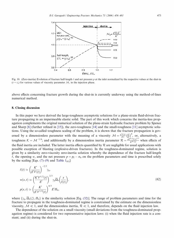
Fig. 10. (Zero-inertia) Evolution of fracture half-length ‘ and net pressure p at the inlet normalized by the respective values at the shut-in(t = t

*) for various values of viscosity parameter M in the injection phase.


above effects concerning fracture growth during the shut-in is currently underway using the method-of-linesnumerical method.

8. Closing discussion

In this paper we have derived the large-toughness asymptotic solutions for a plane-strain fluid-driven frac-ture propagating in an impermeable elastic solid. The part of this work which concerns the inertia-less prop-agation complements the original numerical solution of the plane-strain hydraulic fracture problem by Spenceand Sharp [6] (further refined in [15]), the zero-toughness [14] and the small-toughness [11] asymptotic solu-tions. Using the so-called toughness scaling of the problem, it is shown that the fracture propagation is gov-

erned by a dimensionless parameter with the meaning of a viscosity M ¼ l0V ðtÞE0t

E0

K 0

4, or, alternatively, a

toughness K ¼ M1=4; and additionally by a dimensionless inertia parameter R ¼ qE05=3V ðtÞ5=3

K 08=3t2when effects of

the fluid inertia are included. The latter inertia effects quantified byR are negligible for usual applications withpossible exception of blasting (explosive-driven fractures). In the toughness-dominated regime, solution isgiven by a similarity zero-viscosity zero-inertia solution whereby the dependence of the fracture half-length‘, the opening w, and the net pressure p = pf r0 on the problem parameters and time is prescribed solelyby the scaling [Eqs. (7)–(9) and Table 1(k)]:

‘ðtÞ ’ K 0

E0V ðtÞ

2=3

c0;

wðx; tÞ ’ K 0V 1=2ðtÞE0

2=3

c0X0

x‘ðtÞ

;

pðx; tÞ ’ K 0

E0V 1=4ðtÞ

4=3

E0P0;

ð62Þ

where fc0;X0ðnÞ;P0g is the similarity solution [Eq. (32)]. The range of problem parameters and time for thefracture to propagate in the toughness-dominated regime is constrained by the estimate on the dimensionlessviscosity, M 1, and the dimensionless inertia, R 1, and therefore, depends on the fluid injection law.

The dependence of the solution on a small viscosity (small deviations from the toughness-dominated prop-agation regime) is considered for two representative injection laws: (i) when the fluid injection rate is a con-stant; and (ii) during the shut-in.

0.001 0.01 0.1 1 10

crac

k le

ngth

, (E

'V(t

)/K

')-2/3

0.4

0.6

0.8

1.0

3 4viscosity, ( )E K V t tµ −′ ′ ′= ×

Fig. 11. (Zero-inertia) Dependence of dimensionless crack half-length on dimensionless viscosity M for a constant injection rate: (i) zero-viscosity and zero-toughness [14] solutions are shown by dashed lines; (ii) improved small viscosity and small-toughness [11] asymptoticsolutions are shown by solid lines; and (iii) numerical finite toughness solution [15] is shown by open circles. Triangles show evolution ofthe shut-in solution with diminishing viscosity parameter M ¼ M

tt for two initial values, M ¼ f0:01; 0:03g towards the toughness-

dominated regime, M ’ 0.


8.1. Constant injection rate

In this case, we suggested a method of asymptotic series expansions which allows to study small effects offluid viscosity or/and fluid inertia on the otherwise zero-viscosity, zero-inertia solution of the toughness-dom-inated regime of fracture propagation. The small-viscosity ðM 1Þ similarity expansion of the zero-inertiasolution allows to establish condition M < M0 with M0 ’ 3:4 103 (1% departure from the zero-viscositysolution [Eq. (62)]) which defines a constraint on the solid parameters, fluid viscosity, and fluid injection rateunder which viscosity is irrelevant for fluid-driven fracture propagation (toughness-dominated regime). Thelatter threshold M0 ’ 3:4 103 and the threshold M1 ’ 4:16 for the viscosity-dominated regimeM > M1 (1% departure from the zero-toughness solution, see [11]) provide the parametric rangeM 2 ðM0; M1Þ where both the toughness and the viscosity influence the propagation of a hydraulic fracture.

Fig. 11 shows the variation of the dimensionless fracture length in the toughness scaling with the dimen-sionless viscosity M, in

• the small-toughness asymptotic solution,3

3 Co

c ¼ M1=6ðc0 þ EðM1=4Þc1Þ
with c0 ’ 0.6152, c1 ’ 0.1754,and EðKÞ ¼ 0:1K3:18 is the small-toughness ðK ¼ M1=4Þ parameter [11];and
• the improved small-viscosity asymptotic solution,

c ¼ c0 þ dðMÞc1 with dðMÞ ¼ Mð1þM=MsiÞ1=2

and c0 ’ 0.9324, c1 ’ 2.7220, and Msi ’ 0:0333. The finite toughness numerical solution of Adachi [15] isalso shown in this plot (open circles).

Remarkably, the range of viscosity in which the solution departs from the first-order small-toughness solu-tion and the improved first-order small-viscosity solution is very narrow, 0:2KMK 0:4, see Fig. 11, i.e., thesetwo asymptotes, when combined, effectively approximate the solution in the complete range of the viscosityparameter M.

nverted from the viscosity (m) to the toughness (k) scalings via ck ¼ K2=3cm ¼ M1=6cm [Section 3].


The small-inertia ðRðtÞ 1Þ series expansion of the zero-viscosity solution allows to study the solutiondeparture from the inertia-less regime. In this case, the solution expansion is not self-similar (RðtÞ is a decreas-ing function of time), but each coefficient of the series is. The distribution of the net pressure in the small-iner-tia, zero-viscosity solution shows an increase from the inlet to the tip (an opposite behavior to that of thesmall-viscosity, zero-inertia solution where viscous dissipation in the flow reduces the pressure with the dis-tance in the flow) due to the Bernoullis effect for the flow of inviscid fluid in the crack [17]. Consequently,with increasing inertia, the crack can develop a tear-drop shape with the maximum opening away from thecrack inlet [Fig. 6(a)].

The small-inertia expansion of the zero-viscosity solution and the small-viscosity expansion of the zero-inertia solution can be simply combined to the first order to obtain the OðM;RÞ small viscosity, small inertiasolution. For the dimensionless net pressure we have

Pðn;M;RÞ ¼ P0 þ dðMÞPðlÞ1 ðnÞ þ RPðqÞ

1 ðnÞ ð63Þ
with PðlÞ
1 ðnÞ and PðqÞ1 ðnÞ denote the expressions for the corresponding first-order term P1(n) in [Eq. (41)] and

[Eqs. (C.9)–(C.11)], respectively. Given that the viscosity term PðlÞ1 ðnÞ and the inertia term PðqÞ

1 ðnÞ in [Eq. (63)]decreases and increases in the direction of the flow, respectively. An investigation of Eq. (63) then shows that ifthe effect of the inertia is comparable to or exceeds the effect of the viscosity ðR > 3

2p2=3dðMÞÞ the net pressure

develops a non-monotonic profile with the maximum in the interior of the crack.

8.2. Shut-in

During the shut-in (following an injection), the large-time limit corresponds to an immobile fracture givenby the zero-viscosity zero-inertia solution [Eq. (62)] for a constant injected volume V(t P t*) = V(t*). Evolu-tion of the large-toughness solution from the shut-in instant towards the large-time limit corresponds to aslowing fracture and vanishing effect of the viscosity in time. Fig. 11 illustrates the convergence of the shut-in solution for the crack length (shown by triangles) towards the toughness-dominated limit. The extent offracture propagation during the shut-in D‘ as a fraction of the length ‘* at the end of injection phase, is givenby D‘=‘ ’ 2:9M. The latter is a small fraction for the considered case of a fracture initially propagating inthe large-toughness (small-viscosity) parametric regime, i.e., when M is small. However, much greater extentof the shut-in propagation is anticipated for fractures which propagation during the injection phase is char-acterized by smaller values of the dimensionless toughness. This effect can be partly offset by a progressivefluid leak-off into the permeable rock in field hydraulic fracturing applications, but can be expected to beprominent for tight reservoir rocks or in the hydrofrac laboratory tests in impermeable materials (e.g., PMMA[16]). The transient shut-in solution with the fluid leak-off in arbitrary parametric regime (not confined to thelarge-toughness case) would constitute an interesting problem for the future work.

Acknowledgements

Acknowledgement is made to the Donors of The Petroleum Research Fund, administered by the AmericanChemical Society, for partial support of this research under Grant ACS-PRF 36729-G2. The author is gratefulto Emmanuel Detournay and Jose I. Adachi for interesting discussions and thorough review of the early ver-sion of this manuscript, and to the anonymous reviewer for the comment which led to the improvement of thesmall-viscosity series.

Appendix A. Closed-form expression for DX1ðnÞ, Eq. (37)

In this Appendix we provide details of the calculation of the integral expression for DX1ðnÞ, defined in Eq.(37)b, with DP1(n) given in Eq. (36)b. This integral can be decomposed into two integrals corresponding to thetwo terms in DP1(n) [Eq. (36)b],

DX1ðnÞ ¼8

3p2=3IlnðfÞ

3

4IcosðfÞ

f ¼


q ðA:1Þ


with Iln(f) and Icos(f) given by

IlnðfÞ ¼ 4

p

Z 1

0

Gðf; f0Þ ln f0 dffiffiffiffiffiffiffiffiffiffiffiffiffi1 f02

q; ðA:2Þ

IcosðfÞ ¼4

p

Z 1

0

Gðf; f0Þsin1f0 df0; ðA:3Þ

where the substitution f0 ¼ffiffiffiffiffiffiffiffiffiffiffiffiffiffi1 n02

phas been used. The kernel Gðf; f0Þ is given by

Gðf; f0Þ ¼ Gffiffiffiffiffiffiffiffiffiffiffiffiffi1 f2

q;

ffiffiffiffiffiffiffiffiffiffiffiffiffi1 f02

q ¼ ln

fþ f0

f f0

.

At first, let us consider the integral Iln(f), which can be decomposed as

IlnðfÞ ¼ Ið1Þln ðfÞ þ Ið2Þln ðfÞ; ðA:4Þ

Ið1Þln ðfÞ ¼4

p

Z 1

0

lnfþ f0

f f0


pf0

df0; Ið2Þln ðfÞ ¼8fp

Z 1

0

ln f0ffiffiffiffiffiffiffiffiffiffiffiffiffi1 f02

pf2 f02

df0.

Differentiating integral Ið1Þln ðfÞ with respect to the parameter f and then carrying out the integration in f 0 yieldsdI

ð1Þln =df ¼ 4. Consequently, the integral can be expressed as I

ð1Þln ðfÞ ¼ 4ð1 fÞ þ I

ð1Þln ð1Þ, where I

ð1Þln (1) is a yet

unknown constant. Integration by parts and further simplifications result in Ið1Þln ð1Þ ¼ 2p 4. Summarizing,

Ið1Þln ðfÞ ¼ 2p 4f. ðA:5Þ
The second term Ið2Þln ðfÞ in the expression for Iln(f) is first integrated by parts which upon some algebra resultsin
Ið2Þln ðfÞ ¼ 8

pfJ1

4

p


qJ2ðfÞ; ðA:6Þ

J1 ¼Z 1

0

sin1f0

f0df0 ¼ p ln 4

4; ðA:7Þ

J2ðfÞ ¼Z 1

0

lnfþ f0

f f01 ff0 þ


p ffiffiffiffiffiffiffiffiffiffiffiffiffi1 f02

p1þ ff0 þ


p ffiffiffiffiffiffiffiffiffiffiffiffiffi1 f02

p

df0

f0. ðA:8Þ

Integral J2(f) upon the substitution f ¼ sin a and f0 ¼ sin a0, and some algebra becomes

J2ðaÞ ¼ J2ðsin aÞ ¼Z p=2

0

cot a0 lnsinðaþ a0Þsinða a0Þ

da0. ðA:9Þ

Differentiation of the integral J2ðaÞ with respect to the parameter a and further integration yieldsdJ2ðaÞ=da ¼ p. Utilizing the known value of J2 at a = p/2, J2ðp=2Þ ¼ 0, see Eq. (A.9), we finally obtain

J2ðfÞ ¼ pcos1f. ðA:10Þ
Lastly, let us consider Icos(f). Differentiating with respect to the parameter f, and carrying out the integration,yields dIcos(f)/df = 2ln [4(1 f2)]. Utilizing condition Icos(0) = 0, we obtain
IcosðfÞ ¼ 2 2ð1 ln 2Þfþ lnð1þ fÞ1þf

ð1 fÞ1f

" # !. ðA:11Þ

Substitution of Eqs. (A.11) and (A.4) with (A.5) and (A.6) into Eq. (A.1) yields the final expression

DX1 ¼8

3p2=32p 4nsin1n ð1þ 7 ln 2Þ


q 3

2ln

1þffiffiffiffiffiffiffiffiffiffiffiffiffi1 n2

p 1þ ffiffiffiffiffiffiffi1n2

p

ð1ffiffiffiffiffiffiffiffiffiffiffiffiffi1 n2

pÞ1

ffiffiffiffiffiffiffi1n2

p

2664

3775

0BB@

1CCA. ðA:12Þ

1/j

-400.0 0.1 0.2 0.3 0.4 0.5 0.6

-35

-30

-25

-20

-15

-10

-5

0

1si(2 )S −

1si 33.3−

1

j

j

γγ −

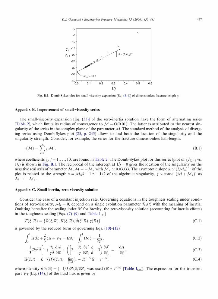
Fig. B.1. Domb-Sykes plot for small viscosity expansion [Eq. (B.1)] of dimensionless fracture length c.


Appendix B. Improvement of small-viscosity series

The small-viscosity expansion [Eq. (33)] of the zero-inertia solution have the form of alternating series[Table 2], which limits its radius of convergence to M ¼ Oð0:01Þ. The latter is attributed to the nearest sin-gularity of the series in the complex plane of the parameter M. The standard method of the analysis of diverg-ing series using Domb-Sykes plot [25, p. 245] allows to find both the location of the singularity and thesingularity strength. Consider, for example, the series for the fracture dimensionless half-length,

cðMÞ ¼X1j¼0

cjMj; ðB:1Þ

where coefficients cj, j = 1, . . . , 10, are found in Table 2. The Domb-Sykes plot for this series (plot of cj/cj1 vs.1/j) is shown in Fig. B.1. The reciprocal of the intercept at 1/j = 0 gives the location of the singularity on thenegative real axis of parameterM,M ¼ Msi withMsi ’ 0:03333. The asymptotic slope S ’ ð2MsiÞ1 of theplot is related to the strength a ¼ MsiS 1 ’ 1=2 of the algebraic singularity, c const ðMþMsiÞa asM ! Msi.

Appendix C. Small inertia, zero-viscosity solution

Consider the case of a constant injection rate. Governing equations in the toughness scaling under condi-tions of zero-viscosity, Mk ¼ 0, depend on a single evolution parameter RkðtÞ with the meaning of inertia.Omitting hereafter the scaling index k for brevity, the zero-viscosity solution (accounting for inertia effects)in the toughness scaling [Eqs. (7)–(9) and Table 1(k)]

Fðn;RÞ ¼ Xðn;RÞ;Pðn;RÞ; #ðn;RÞ; cðRÞ

ðC:1Þ

is governed by the reduced form of governing Eqs. (10)–(12)
Z 1
nXdnþ 2

3nXþWT ¼ X #;

Z 1

0

Xdn ¼ 1

2c2; ðC:2Þ

1

3Rc2 # 1þ R

c #

oc #oR þ 2R

cocoR

n# 3

o #

on

¼ oP

on; ðC:3Þ

Xðn; tÞ ¼ L1fPgðn; tÞ; limn!1

ð1 nÞ1=2X ¼ c1=2; ðC:4Þ

where identity tðo=otÞ ¼ ð1=3ÞRðo=oRÞ was used (R t1=3 [Table 1(k)]). The expression for the transientpart WT [Eq. (14)a] of the fluid flux is given by

4 Asor of awhen n


WT ¼ 1

3

Z 1

nR oX

oRþRc

ocoR X n

oXon

dn; ðC:5Þ

while the expression for the transient part UT [Eq. (14)b] in the momentum equation has been used with theabove identity to arrive to Eq. (C.3).

The above system of equations explicitly depends on the evolving-in-time parameter R , and, therefore, itsgeneral solution (except for the zero and the infinite limits of R) cannot be self-similar.4 The limit of zero iner-tia, R ¼ 0, constitutes a self-similar limit given by Eq. (32). Since the effect of the fluid inertia quantified by Rdecreases with time, the above limit corresponds to the large-time asymptote of a fracture driven by an inviscidfluid. The transition towards this self-similar limit can be studied using the perturbation method of Section 6.1.

Substituting small inertia expansion [Eq. (44)] into Eqs. (C.2)–(C.5) and collecting terms of the same orderin R yield equations for the expansion terms to any given order. In constructing expansions for the governingequations, the care should be exercised in evaluating expansions for the transient terms, e.g.,

Rc

ocoR ¼ c1

c0Rþ 2c2

c0 c21c20

R2 þOðR3Þ.

The contribution of transient terms in lubrication Eq. (C.3) is OðR2Þ, consequently, the equations governingthe OðRÞ term in the expansion are particularly simple

1

X0

Z 1

nX0 dnþ

2

3n ¼ #0; c1 ¼ c30

Z 1

0

X1 dg; ðC:6Þ

1

3c20 #0 1þ 2

n#0

3

d #0

dn

¼ dP1

dn; ðC:7Þ

X1ðnÞ ¼ L1fP1gðnÞ; limn!1

ð1 nÞ1=2X1 ¼ 1

2c1c

3=20 . ðC:8Þ

Substitution of the expression for #0 following from Eq. (C.6)a into Eq. (C.7) and integration yields the pres-sure term profile

P1 ¼ P1ð0Þ þ DP1ðnÞ with ðC:9Þ

DP1ðnÞ ¼1

6p4=3

p2

4þ 5n2

3þ 6ncos1nffiffiffiffiffiffiffiffiffiffiffiffiffi

1 n2p ð1þ 2n2Þðcos1nÞ2

1 n2

!; ðC:10Þ

where the inlet value P1(0) is unknown. Corresponding expression for the opening term X1 ¼ L1fP1g is ofthe form (37). Following the treatment of Section 6.1 we can obtain the solution constants as follows:

P1ð0Þ ¼ 21p2 13

216p4=3’ 0:19546; ðC:11Þ

c1 ¼4ð6p2 43Þ

27p7=3’ 0:16621. ðC:12Þ

Similarly, we obtain the higher order terms in the expansion (44). The integrals arising in the evaluation of theelasticity and the lubrication equations for successive expansion terms increase in complexity, and, therefore,are implemented numerically. The results for the terms in the inertia expansion of the zero-viscosity solutionup to the OðR5Þ for the crack length c, the inlet, P(0), and the tip, P(1), values of the net pressure, and theinlet normalized opening Xð0Þ are summarized in Table C.1. Profiles of the opening and the pressure terms inthe inertia expansion of the zero-viscosity solution (44) are shown in Fig. C.1.

discussed in Section 3, a self-similar solution exists when the injection rate is increasing with time as _V t1=5. The treatment of thisny other power law injection case, _V ta with a > 0, is identical to the treatment of a constant injection rate case considered hereumerical coefficients in Eqs. (C.2)a and (C.3) are modified accordingly.

Table C.1Numerical values of coefficients of the OðRjÞ terms, j = 0,1, . . . ,5, in the expansion [Eq. (44)] of crack half-length c, net pressure at theinlet, P(0), net pressure at the tip, P(1), and normalized opening Xð0Þ at the inlet

cj Pj(0) Pj(1) Xjð0Þj = 0 0.93239 0.18307 0.18307 0.73229j = 1 0.16621 0.19546 0.062952 0.376464j = 2 0.154028 0.144179 0.0301009 0.259143j = 3 0.200661 0.205116 0.028148 0.324525j = 4 0.305301 0.381546 0.0280604 0.517134j = 5 0.502836 0.816739 0.0168989 0.936821

ξ

-1.0-0.8-0.6-0.4-0.20.0

0.0 0.2 0.4 0.6 0.8 1.0

ξ0.0 0.2 0.4 0.6 0.8 1.0

0.20.40.60.81.0

Π

-1.0

-0.5

0.0

0.5

(a) (b)

Ω

0Ω0Π

1Ω1Π

5Π

5Ω4Ω

2Ω

2Π

4Π

Fig. C.1. (Constant injection rate, zero-viscosity) Zero- to the fifth-order inertia terms of normalized opening, (a), and net-pressure, (b), insmall inertia expansion of the zero-viscosity solution.


Appendix D. Method of lines numerical approach

A general method-of-lines numerical approach [26–28] is used to solve the system of coupled Eqs. (52), (53),(59), (60), and (58) for the regular parts dPðn; sÞ and dWðn; sÞ of the pressure and opening terms, respectively,and crack length exponent A(s ). The method of lines as applied here essentially corresponds to a discretizationof the solution in space, but not in time, such that the governing equations reduce to a system of coupledODEs in time. This system governs the evolution of the values of the solution at a discrete set of points inthe space interval along the crack.

First, a set of fixed grid points ni, i = 1, . . . ,M with n1 = 0 and nM = 1 is selected. (Even though a uniformgrid spacing is used in the computation of the final results, the development below does not make this assump-tion.) The regular function dPðn; sÞ is then approximated by a piecewise linear function defined by its valuesfdPiðsÞg at the grid points ni

dPðn; sÞ ’ dPiðsÞ þdPiþ1ðsÞ dPiðsÞ

niþ1 nin nið Þ; n 2 ½ni; niþ1Þ. ðD:1Þ

The corresponding expression for dWðn; sÞ is given by the elasticity integral [Eq. (60)a], computed explicitly forthe piecewise linear distribution of dP [Eq. (D.1)]

dWðn; sÞ ¼XM1

i¼1

½Iaðn; n0ÞaiðsÞ þ Ibðn; n0ÞbiðsÞn0¼niþ1

n0¼ni. ðD:2Þ

In the above expression ai(s) and bi(s) are given by

ai ¼ dPi dPiþ1 dPi

niþ1 nini; bi ¼

dPiþ1 dPi

niþ1 ni; ðD:3Þ

and the functions Ia,b(n, n 0) are defined as follows:


Iaðn; n0Þ ¼4

p

Z n0

G n; n0ð Þdn0

¼ 4

p2


qsin1n0 þ n0 ln


pþ


pffiffiffiffiffiffiffiffiffiffiffiffiffiffi1 n02

p


p

þ n lnn n0

nþ n01þ nn0 þ


p ffiffiffiffiffiffiffiffiffiffiffiffiffi1 n2

p1 nn0 þ


p ffiffiffiffiffiffiffiffiffiffiffiffiffi1 n2

p

!; ðD:4Þ

Ibðn; n0Þ ¼4

p

Z n0

Gðn; n0Þn0dn0 ¼ 4

p


q ffiffiffiffiffiffiffiffiffiffiffiffiffi1 n2

qþ n02 n2

2ln


pþ


pffiffiffiffiffiffiffiffiffiffiffiffiffiffi1 n02

p


p

!

. ðD:5Þ

With the help of Eqs. (57) and (D.2), an expression for the function U ¼ cos1nþ 4p

R 1

n W dn in the lubricationEq. (53)a is given by

Uðn;sÞ¼ cos1nþ 4

pAðsÞAð0Þ

1

c1

Z 1

nX1ðnÞdnþ

XM1

i¼1

½Jað1;n0Þ Jaðn;n0ÞaiðsÞþ ½Jbð1;n0Þ Jbðn;n0ÞbiðsÞ½ n0¼niþ1

n0¼ni

!.

ðD:6Þ
Lengthy closed-form expressions for the functions Ja,b(n, n 0) = nIa,b(n, n 0)dn and
R 1

n X1ðnÞdn are omitted herefor brevity.

Substitution of Eq. (D.6) into the lubrication Eq. (53)a and its evaluation at the mid-points ni+1/2 =(ni + ni+1)/2 (i = 1, . . . ,M 1) of the grid elements yields a system of M 1 coupled ordinary differentialequations

4

p

_AðsÞc1Að0Þ

Z 1

nX1ðnÞdnþ

XM1

i¼1

½Jað1; n0Þ Jaðn; n0Þ _aiðsÞ þ ½Jbð1; n0Þ Jbðn; n0Þ _biðsÞ n0¼niþ1

n0¼ni

!

¼ 2ð1 n2Þ3=2 AðsÞAð0Þ

1

c1

dP1

dnþ biðsÞ

AðsÞUðn; sÞ; n ¼ niþ1=2; ðD:7Þ

on M + 1 unknowns: A(s), dP1ðsÞ; . . . ; dPMðsÞ. (Note that in Eq. (D.7), U is given by Eq. (D.6) and ai, bi aredefined in terms of fdPig by Eq. (D.3).)

Two additional equations of the linear algebraic form are provided by the global continuity condition,Ujn=0 = 0, Eq. (59), with (D.6) and (D.3), and the tip condition [Eq. (60)b]. The latter, given the propertiesof the functions Ia,b(n, n 0) [Eqs. (D.4) and (D.5)], has the form

XM1

i¼1

½Iaðn0ÞaiðsÞ þ Ibðn0ÞbiðsÞn0¼niþ1

n0¼ni¼ p

25=2AðsÞAð0Þ 1

; ðD:8Þ

where Ia;bðn0Þ ¼ limn!1ð1 nÞ1=2Ia;bðn; n0Þ,

Iaðn0Þ ¼8ffiffiffi2

p

psin1n0; Ibðn0Þ ¼ 8

ffiffiffi2

p

p


q.

These two linear algebraic relations are used to reduce the number of unknowns in Eq. (D.7), i = 1, . . . ,M 1,by two (e.g., by expressing A(s) and dP1ðsÞ in terms of dP2ðsÞ; . . . ; dPMðsÞ).

Initial conditions are provided by Eq. (58) in the form

dPið0Þ ¼ 0; i ¼ 1; . . . ;M . ðD:9Þ
Summarizing, the system of M 1 ODEs [Eq. (D.7)] plus two linear algebraic relations [Eqs. (59) and (D.8)],and initial conditions [Eq. (D.9)] is solved numerically for A(s) and dP1ðsÞ; . . . ; dPMðsÞ by means of the ODEsolver in the software Mathematica, version 4.1 ( 1988–2000 Wolfram Research, Inc.).
The self-similar ‘‘large-time’’ asymptote of the above solution can be obtained either as the large-time limitof the above numerical solution or can be solved directly. Indeed, this limit solution is time-independent (i.e.,A and dP1; . . . ; dPM are asymptotic constants) and the right hand side of the lubrication Eq. (D.7) evaluated at


the grid element midpoint, n = ni+1/2, is zero. Thus, Eqs. (D.7), (59), and (D.8) yield a system of algebraicequations on M + 1 unknown constants A and dP1; . . . ; dPM . This algebraic system is solved numericallyusing Mathematica, which utilizes a damped Newtons method, the secant method and Brents method.

References

[1] Economides MJ, Nolte KG, editorsReservoir stimulation. 3rd ed. Chichester, UK: John Wiley & Sons; 2000.[2] Spence DA, Turcotte DL. Magma-driven propagation of cracks. J Geophys Res 1985;90:575–80.[3] Detournay E, Garagash DI. The tip region of a fluid-driven fracture in a permeable elastic solid. J Fluid Mech 2003;494:1–32.[4] Nilson RH. Gas driven fracture propagation. ASME J Appl Mech 1981;48:757–62.[5] Nilson RH. Similarity solutions for wedge-shaped hydraulic fracture driven into a permeable medium by a constant inlet pressure. Int

J Numer Anal Methods Geomech 1988;12:477–95.[6] Spence DA, Sharp PW. Self-similar solution for elastohydrodynamic cavity flow. Proc Roy Soc London, Ser A 1985(400):289–313.[7] Lister JR. Buoyancy-driven fluid fracture: The effects of material toughness and of low-viscosity precursors. J Fluid Mech

1990;210:263–80.[8] Carbonell RS, Desroches J, Detournay E. A comparison between a semi-analytical and a numerical solution of a two-dimensional

hydraulic fracture. Int J Solids Struct 1999;36(31–32):4869–88.[9] Garagash DI. Hydraulic fracture propagation in elastic rock with large toughness. In: Girard J, Liebman M, Breeds C,

Doe T, editors. Rock around the rim—proceedings of the 4th North American rock mechanics symposium. Rotterdam: Balkema;2000. p. 221–8.

[10] Savitski AA, Detournay E. Propagation of a fluid-driven penny-shaped fracture in an impermeable rock: Asymptotic solutions. Int JSolids Struct 2002;39(26):6311–37.

[11] Garagash DI, Detournay E. Plane-strain propagation of a fluid-driven fracture: small toughness solution. ASME J Appl Mech2005;72:916–28.

[12] Detournay E. Fluid and solid singularities at the tip of a fluid-driven fracture. In: Detournay D, Pearson JRA, editors.Proceedings of the IUTAM symposium on non-linear singularities in deformation and flow, Haifa. Dordrecht: Kluwer AcademicPubl.; 1999. p. 27–42.

[13] Garagash DI, Detournay E. Viscosity-dominated regime of a fluid-driven fracture in an elastic medium. In: Karihaloo BL, editor.IUTAM symposium on analytical and computational fracture mechanics of non-homogeneous materials, Cardiff. Solid mechanicsand its applications, vol. 97, March 2002. p. 25–9.

[14] Adachi JI, Detournay E. Self-similar solution of a plane-strain fracture driven by a power-law fluid. Int J Numer Anal MethodsGeomech 2002;26:579–604.

[15] Adachi JI. Fluid-driven fracture in permeable rock. PhD thesis, University of Minnesota, 2001.[16] Bunger AP, Detournay E, Jeffrey RG. Crack tip behavior in near-surface fluid-driven fracture experiments. CR Acad Sci Paris

2005;333:299–304.[17] Huang N, Szewczyk A, Li Y. Self-similar solution in problems of hydraulic fracturing. ASME J Appl Mech 1990;57:877–81.[18] Batchelor GK. An introduction to fluid dynamics. Cambridge, UK: Cambridge University Press; 1967.[19] Rice JR. Mathematical analysis in the mechanics of fracture. In: Liebowitz H, editor. Fracture, an advanced treatise, vol. II. New

York, NY: Academic Press; 1968. p. 191–311 [Chapter 3].[20] Papanastasiou P. The effective fracture toughness in hydraulic fracturing. Int J Fracture 1999;96:127–47.[21] Shapiro RA. The dynamics and thermodynamics of compressible fluid flow, vol. II. New York: Ronald Press; 1954.[22] Sneddon IN, Lowengrub M. Crack problems in the classical theory of elasticity. New York, NY: John Wiley & Sons; 1969.[23] Nilson RH, Morrison FA. Transient gas or liquid flow along a preexisting or hydraulically-induced fracture in permeable medium.

ASME J Appl Mech 1986;53:157–65.[24] Detournay E. Propagation regimes of fluid-driven fractures in impermeable rocks. Int J Geomech 2004;4(1):1–11.[25] Van Dyke M. Perturbation methods in fluid mechanics. Stanford: Parabolic Press; 1975.[26] Liskovets OA. The method of lines. J Differ Eqs 1965;1:1308.[27] Nilson RH, Griffiths SK. Numerical analysis of hydraulically-driven fractures. Comput Methods Appl Mech Eng 1983;36:359–70.[28] Garagash DI, Detournay E. An analysis of the influence of the pressurization rate on the borehole breakdown pressure. Int J Solids

Struct 1997;34(24):3099–118.

Documents

06-Garagash Large Toughness