Embed Size (px)
DESCRIPTION
MI BOOK ALONG WITH MRS PPT.........GAURAV GAVE ME SO I UPLOADED IT
Citation preview

This page intentionally left blank
Introduction to Medical ImagingPhysics, Engineering and Clinical Applications
Covering the basics of X-rays, CT, PET, nuclear medicine, ultrasound and MRI, thistextbook provides senior undergraduate and beginning graduate students with a broadintroduction to medical imaging. Over 130 end-of-chapter exercises are included, inaddition to solved example problems, which enable students to master the theory as wellas providing them with the tools needed to solve more difficult problems. The basictheory, instrumentation and state-of-the-art techniques and applications are covered,bringing students immediately up-to-date with recent developments, such as combinedcomputed tomography/positron emission tomography, multi-slice CT, four-dimensionalultrasound and parallel imaging MR technology. Clinical examples provide practicalapplications of physics and engineering knowledge to medicine. Finally, helpful refer-ences to specialized texts, recent review articles and relevant scientific journals areprovided at the end of each chapter, making this an ideal textbook for a one-semestercourse in medical imaging.
Nadine Barrie Smith is a faculty member in the Bioengineering Department and theGraduate Program in Acoustics at Pennsylvania State University. She also holds avisiting faculty position at the Leiden University Medical Center. She is a Senior Memberof the IEEE, and of the American Institute of Ultrasound in Medicine where she is onboth the Bioeffects and Technical Standards Committees. Her current research involvesultrasound transducer design, ultrasound imaging and therapeutic applications of ultra-sound. She has taught undergraduate medical imaging and graduate ultrasound imagingcourses for the past 10 years.
Andrew Webb is Professor of Radiology at the Leiden University Medical Center, andDirector of the C.J. Gorter High Field Magnetic Resonance Imaging Center. He is aSenior Member of the IEEE, and a Fellow of the American Institute of Medical andBiological Engineering. His research involves many areas of high field magnetic reso-nance imaging. He has taught medical imaging classes for graduates and undergraduatesboth nationally and internationally for the past 15 years.
Cambridge Texts in Biomedical Engineering
Series Editors
W. Mark Saltzman, Yale University
Shu Chien, University of California, San Diego
Series Advisors
William Hendee, Medical College of Wisconsin
Roger Kamm, Massachusetts Institute of Technology
Robert Malkin, Duke University
Alison Noble, Oxford University
Bernhard Palsson, University of California, San Diego
Nicholas Peppas, University of Texas at Austin
Michael Sefton, University of Toronto
George Truskey, Duke University
Cheng Zhu, Georgia Institute of Technology
Cambridge Texts in Biomedical Engineering provides a forum for high-quality accessible
textbooks targeted at undergraduate and graduate courses in biomedical engineering. It
covers a broad range of biomedical engineering topics from introductory texts to
advanced topics including, but not limited to, biomechanics, physiology, biomedical
instrumentation, imaging, signals and systems, cell engineering, and bioinformatics. The
series blends theory and practice, aimed primarily at biomedical engineering
students, it also suits broader courses in engineering, the life sciences and medicine.

Introduction toMedical ImagingPhysics, Engineering andClinical Applications
Nadine Barrie SmithPennsylvania State University
Andrew WebbLeiden University Medical Center

cambridge university press
Cambridge, New York, Melbourne, Madrid, Cape Town, Singapore,Sao Paulo, Delhi, Dubai, Tokyo, Mexico City
Cambridge University PressThe Edinburgh Building, Cambridge CB2 8RU, UK
Published in the United States of America by Cambridge University Press, New York
www.cambridge.orgInformation on this title: www.cambridge.org/9780521190657
� N. Smith and A. Webb 2011
This publication is in copyright. Subject to statutory exceptionand to the provisions of relevant collective licensing agreements,no reproduction of any part may take place without the writtenpermission of Cambridge University Press.
First published 2011
Printed in the United Kingdom at the University Press, Cambridge
A catalogue record for this publication is available from the British Library
Library of Congress Cataloging-in-Publication Data
Webb, Andrew (Andrew G.)Introduction to medical imaging : physics, engineering, and clinicalapplications / Andrew Webb, Nadine Smith.
p. ; cm.Includes bibliographical references and index.ISBN 978-0-521-19065-7 (hardback)1. Diagnostic imaging. 2. Medical physics. I. Smith, Nadine, 1962–2010.II. Title.[DNLM: 1. Diagnostic Imaging. WN 180]
RC78.7.D53.W43 2011616.07#54–dc22 2010033027
ISBN 978-0-521-19065-7 Hardback
Additional resources for this publication at www.cambridge.org/9780521190657
Cambridge University Press has no responsibility for the persistenceor accuracy of URLs for external or third-party internet websites referredto in this publication, and does not guarantee that any contenton such websites is, or will remain, accurate or appropriate.

‘‘This is an excellently prepared textbook for a senior/first year graduate level course.
It explains physical concepts in an easily understandable manner. In addition, a problem
set is included after each chapter. Very few books on the market today have this choice.
I would definitely use it for teaching a medical imaging class at USC.’’
K. Kirk Shung, University of Southern California
‘‘I have anxiously anticipated the release of this book and will use it with both students
and trainees.’’
Michael B. Smith, Novartis Institutes for Biomedical Research
‘‘An excellent and approachable text for both undergraduate and graduate student.’’
Richard Magin, University of Illinois at Chicago

Contents
1 General image characteristics, data acquisitionand image reconstruction
1
1.1 Introduction 11.2 Specificity, sensitivity and the receiver operating
characteristic (ROC) curve2
1.3 Spatial resolution 51.3.1 Spatial frequencies 51.3.2 The line spread function 61.3.3 The point spread function. 71.3.4 The modulation transfer function 8
1.4 Signal-to-noise ratio 101.5 Contrast-to-noise ratio 121.6 Image filtering 121.7 Data acquisition: analogue-to-digital converters 15
1.7.1 Dynamic range and resolution 161.7.2 Sampling frequency and bandwidth 181.7.3 Digital oversampling 19
1.8 Image artifacts 201.9 Fourier transforms 20
1.9.1 Fourier transformation of time- and spatialfrequency-domain signals
21
1.9.2 Useful properties of the Fourier transform 221.10 Backprojection, sinograms and filtered backprojection 24
1.10.1 Backprojection 261.10.2 Sinograms 271.10.3 Filtered backprojection 27
Exercises 30
2 X-ray planar radiography and computed tomography 34
2.1 Introduction 342.2 The X-ray tube 362.3 The X-ray energy spectrum 40
2.4 Interactions of X-rays with the body 422.4.1 Photoelectric attenuation 422.4.2 Compton scattering 43
2.5 X-ray linear and mass attenuation coefficients 452.6 Instrumentation for planar radiography 47
2.6.1 Collimators 482.6.2 Anti-scatter grids 48
2.7 X-ray detectors 502.7.1 Computed radiography 502.7.2 Digital radiography 52
2.8 Quantitative characteristics of planar X-ray images 542.8.1 Signal-to-noise 542.8.2 Spatial resolution 572.8.3 Contrast-to-noise 58
2.9 X-ray contrast agents 592.9.1 Contrast agents for the GI tract 592.9.2 Iodine-based contrast agents 60
2.10 Specialized X-ray imaging techniques 612.10.1 Digital subtraction angiography 612.10.2 Digital mammography 622.10.3 Digital fluoroscopy 63
2.11 Clinical applications of planar X-ray imaging 642.12 Computed tomography 66
2.12.1 Spiral/helical CT 672.12.2 Multi-slice spiral CT 68
2.13 Instrumentation for CT 682.13.1 Instrumentation development for helical CT 692.13.2 Detectors for multi-slice CT 70
2.14 Image reconstruction in CT 712.14.1 Filtered backprojection techniques 712.14.2 Fan beam reconstructions 732.14.3 Reconstruction of helical CT data 732.14.4 Reconstruction of multi-slice helical CT scans 742.14.5 Pre-processing data corrections 74
2.15 Dual-source and dual-energy CT 752.16 Digital X-ray tomosynthesis 762.17 Radiation dose 772.18 Clinical applications of CT 80
2.18.1 Cerebral scans 802.18.2 Pulmonary disease 812.18.3 Liver imaging 812.18.4 Cardiac imaging 82
Exercises 83
viii Contents

3 Nuclear medicine: Planar scintigraphy, SPECTand PET/CT
89
3.1 Introduction 893.2 Radioactivity and radiotracer half-life 913.3 Properties of radiotracers for nuclear medicine 923.4 The technetium generator 933.5 The distribution of technetium-based radiotracers
within the body96
3.6 The gamma camera 973.6.1 The collimator 973.6.2 The detector scintillation crystal and coupled
photomultiplier tubes100
3.6.3 The Anger position network and pulse height analyzer 1033.6.4 Instrumental dead time 106
3.7 Image characteristics 1083.8 Clinical applications of planar scintigraphy 1093.9 Single photon emission computed tomography (SPECT) 1103.10 Data processing in SPECT 112
3.10.1 Scatter correction 1123.10.2 Attenuation correction 1143.10.3 Image reconstruction 115
3.11 SPECT/CT 1163.12 Clinical applications of SPECT and SPECT/CT 117
3.12.1 Myocardial perfusion 1173.12.2 Brain SPECT and SPECT/CT 120
3.13 Positron emission tomography (PET) 1213.14 Radiotracers used for PET/CT 1233.15 Instrumentation for PET/CT 124
3.15.1 Scintillation crystals 1253.15.2 Photomultiplier tubes and pulse height analyzer 1273.15.3 Annihilation coincidence detection 127
3.16 Two-dimensional and three-dimensional PET imaging 1293.17 PET/CT 1303.18 Data processing in PET/CT 131
3.18.1 Attenuation correction 1313.18.2 Corrections for accidental and multiple coincidences 1313.18.3 Corrections for scattered coincidences 1333.18.4 Corrections for dead time 134
3.19 Image characteristics 1343.20 Time-of-flight PET 1353.21 Clinical applications of PET/CT 137
3.21.1 Whole-body PET/CT scanning 137
ix Contents
3.21.2 PET/CT applications in the brain 1373.21.3 Cardiac PET/CT studies 139
Exercises 139
4 Ultrasound imaging 145
4.1 Introduction 1454.2 Wave propagation and characteristic acoustic impedance 1464.3 Wave reflection, refraction and scattering in tissue 149
4.3.1 Reflection, transmission and refraction at tissueboundaries
149
4.3.2 Scattering by small structures 1524.4 Absorption and total attenuation of ultrasound
energy in tissue153
4.4.1 Relaxation and classical absorption 1544.4.2 Attenuation coefficients 155
4.5 Instrumentation 1564.6 Single element ultrasound transducers 157
4.6.1 Transducer bandwidth 1594.6.2 Beam geometry and lateral resolution 1614.6.3 Axial resolution 1634.6.4 Transducer focusing 163
4.7 Transducer arrays 1654.7.1 Linear arrays 1664.7.2 Phased arrays 1674.7.3 Beam-forming and steering via pulse transmission
for phased arrays168
4.7.4 Analogue and digital receiver beam-formingfor phased arrays
171
4.7.5 Time-gain compensation 1724.7.6 Multi-dimensional arrays 1734.7.7 Annular arrays 174
4.8 Clinical diagnostic scanning modes 1754.8.1 A-mode scanning: ophthalmic pachymetry 1754.8.2 M-mode echocardiography 1754.8.3 Two-dimensional B-mode scanning 1764.8.4 Compound scanning 177
4.9 Image characteristics 1784.9.1 Signal-to-noise 1784.9.2 Spatial resolution 1784.9.3 Contrast-to-noise 179
4.10 Doppler ultrasound for blood flow measurements 1794.10.1 Pulsed wave Doppler measurements 1814.10.2 Duplex and triplex image acquisition 182
x Contents
4.10.3 Aliasing in pulsed wave Doppler imaging 1844.10.4 Power Doppler 1864.10.5 Continuous-wave Doppler measurements 186
4.11 Ultrasound contrast agents 1874.11.1 Microbubbles 1874.11.2 Harmonic and pulse inversion imaging 190
4.12 Safety guidelines in ultrasound imaging 1914.13 Clinical applications of ultrasound 193
4.13.1 Obstetrics and gynaecology 1934.13.2 Breast imaging 1944.13.3 Musculoskeletal structure 1944.13.4 Echocardiography 195
4.14 Artifacts in ultrasound imaging 196Exercises 197
5 Magnetic resonance imaging (MRI) 204
5.1 Introduction 2045.2 Effects of a strong magnetic field on protons in the body 205
5.2.1 Proton energy levels 2065.2.2 Classical precession 209
5.3 Effects of a radiofrequency pulse on magnetization 2115.3.1 Creation of transverse magnetization 212
5.4 Faraday induction: the basis of MR signal detection 2135.4.1 MR signal intensity 2145.4.2 The rotating reference frame 214
5.5 T1 and T2 relaxation times 2155.6 Signals from lipid 2195.7 The free induction decay 2205.8 Magnetic resonance imaging 2215.9 Image acquisition 223
5.9.1 Slice selection 2235.9.2 Phase encoding 2265.9.3 Frequency encoding 228
5.10 The k-space formalism and image reconstruction 2295.11 Multiple-slice imaging 2315.12 Basic imaging sequences 233
5.12.1 Multi-slice gradient echo sequences 2335.12.2 Spin echo sequences 2345.12.3 Three-dimensional imaging sequences 237
5.13 Tissue relaxation times 2395.14 MRI instrumentation 241
5.14.1 Superconducting magnet design 241
xi Contents
5.14.2 Magnetic field gradient coils 2445.14.3 Radiofrequency coils 2475.14.4 Receiver design 250
5.15 Parallel imaging using coil arrays 2525.16 Fast imaging sequences 254
5.16.1 Echo planar imaging 2555.16.2 Turbo spin echo sequences 256
5.17 Magnetic resonance angiography 2575.18 Functional MRI 2595.19 MRI contrast agents 261
5.19.1 Positive contrast agents 2615.19.2 Negative contrast agents 263
5.20 Image characteristics 2645.20.1 Signal-to-noise 2645.20.2 Spatial resolution 2655.20.3 Contrast-to-noise 266
5.21 Safety considerations – specific absorption rate (SAR) 2675.22 Lipid suppression techniques 2675.23 Clinical applications 268
5.23.1 Neurological applications 2685.23.2 Body applications 2695.23.3 Musculoskeletal applications 2705.23.4 Cardiology applications 271
Exercises 273
Index 283
xii Contents
1 General image characteristics, dataacquisition and image reconstruction
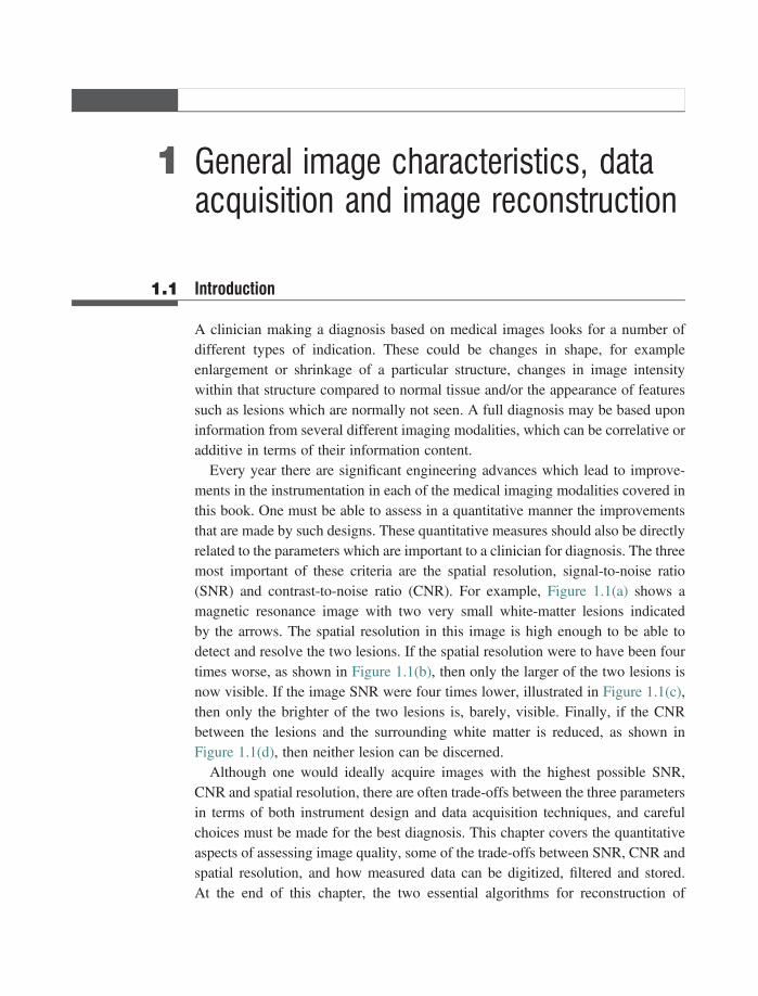
1.1 Introduction
A clinician making a diagnosis based on medical images looks for a number ofdifferent types of indication. These could be changes in shape, for exampleenlargement or shrinkage of a particular structure, changes in image intensitywithin that structure compared to normal tissue and/or the appearance of featuressuch as lesions which are normally not seen. A full diagnosis may be based uponinformation from several different imaging modalities, which can be correlative oradditive in terms of their information content.
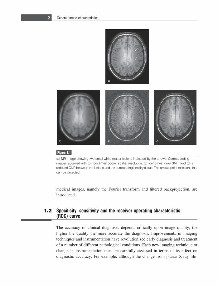
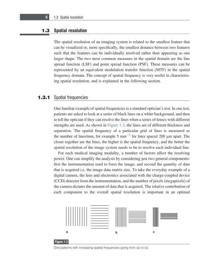
Every year there are significant engineering advances which lead to improve-ments in the instrumentation in each of the medical imaging modalities covered inthis book. One must be able to assess in a quantitative manner the improvementsthat are made by such designs. These quantitative measures should also be directlyrelated to the parameters which are important to a clinician for diagnosis. The threemost important of these criteria are the spatial resolution, signal-to-noise ratio(SNR) and contrast-to-noise ratio (CNR). For example, Figure 1.1(a) shows amagnetic resonance image with two very small white-matter lesions indicatedby the arrows. The spatial resolution in this image is high enough to be able todetect and resolve the two lesions. If the spatial resolution were to have been fourtimes worse, as shown in Figure 1.1(b), then only the larger of the two lesions isnow visible. If the image SNR were four times lower, illustrated in Figure 1.1(c),then only the brighter of the two lesions is, barely, visible. Finally, if the CNRbetween the lesions and the surrounding white matter is reduced, as shown inFigure 1.1(d), then neither lesion can be discerned.
Although one would ideally acquire images with the highest possible SNR,CNR and spatial resolution, there are often trade-offs between the three parametersin terms of both instrument design and data acquisition techniques, and carefulchoices must be made for the best diagnosis. This chapter covers the quantitativeaspects of assessing image quality, some of the trade-offs between SNR, CNR andspatial resolution, and how measured data can be digitized, filtered and stored.At the end of this chapter, the two essential algorithms for reconstruction of
medical images, namely the Fourier transform and filtered backprojection, areintroduced.
1.2 Specificity, sensitivity and the receiver operating characteristic(ROC) curve
The accuracy of clinical diagnoses depends critically upon image quality, thehigher the quality the more accurate the diagnosis. Improvements in imagingtechniques and instrumentation have revolutionized early diagnosis and treatmentof a number of different pathological conditions. Each new imaging technique orchange in instrumentation must be carefully assessed in terms of its effect ondiagnostic accuracy. For example, although the change from planar X-ray film
a
b c d
Figure 1.1
(a) MR image showing two small white-matter lesions indicated by the arrows. Correspondingimages acquired with (b) four times poorer spatial resolution, (c) four times lower SNR, and (d) areduced CNR between the lesions and the surrounding healthy tissue. The arrows point to lesions thatcan be detected.
2 General image characteristics
to digital radiography clearly has many practical advantages in terms of datastorage and mobility, it would not have been implemented clinically had thediagnostic quality of the scans decreased. Quantitative assessment of diagnosticquality is usually reported in terms of specificity and sensitivity, as described in theexample below.
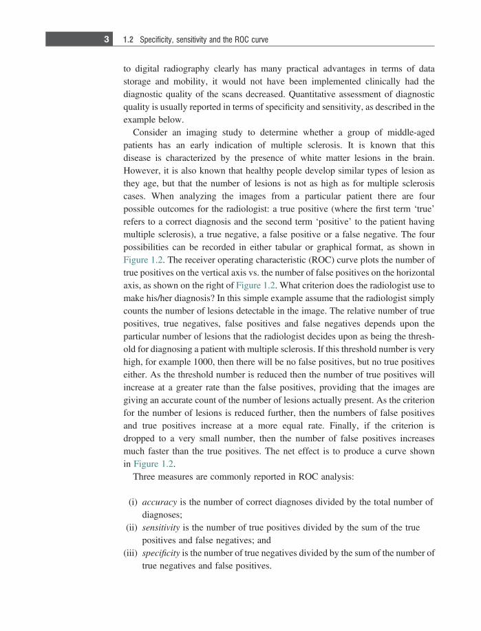
Consider an imaging study to determine whether a group of middle-agedpatients has an early indication of multiple sclerosis. It is known that thisdisease is characterized by the presence of white matter lesions in the brain.However, it is also known that healthy people develop similar types of lesion asthey age, but that the number of lesions is not as high as for multiple sclerosiscases. When analyzing the images from a particular patient there are fourpossible outcomes for the radiologist: a true positive (where the first term ‘true’refers to a correct diagnosis and the second term ‘positive’ to the patient havingmultiple sclerosis), a true negative, a false positive or a false negative. The fourpossibilities can be recorded in either tabular or graphical format, as shown inFigure 1.2. The receiver operating characteristic (ROC) curve plots the number oftrue positives on the vertical axis vs. the number of false positives on the horizontalaxis, as shown on the right of Figure 1.2. What criterion does the radiologist use tomake his/her diagnosis? In this simple example assume that the radiologist simplycounts the number of lesions detectable in the image. The relative number of truepositives, true negatives, false positives and false negatives depends upon theparticular number of lesions that the radiologist decides upon as being the thresh-old for diagnosing a patient with multiple sclerosis. If this threshold number is veryhigh, for example 1000, then there will be no false positives, but no true positiveseither. As the threshold number is reduced then the number of true positives willincrease at a greater rate than the false positives, providing that the images aregiving an accurate count of the number of lesions actually present. As the criterionfor the number of lesions is reduced further, then the numbers of false positivesand true positives increase at a more equal rate. Finally, if the criterion isdropped to a very small number, then the number of false positives increasesmuch faster than the true positives. The net effect is to produce a curve shownin Figure 1.2.
Three measures are commonly reported in ROC analysis:
(i) accuracy is the number of correct diagnoses divided by the total number ofdiagnoses;
(ii) sensitivity is the number of true positives divided by the sum of the truepositives and false negatives; and
(iii) specificity is the number of true negatives divided by the sum of the number oftrue negatives and false positives.
3 1.2 Specificity, sensitivity and the ROC curve
The aim of clinical diagnosis is to maximize each of the three numbers, with anideal value of 100% for all three. This is equivalent to a point on the ROC curvegiven by a true positive fraction of 1, and a false positive fraction of 0. Thecorresponding ROC curve is shown as the dotted line in Figure 1.2. The closerthe actual ROC curve gets to this ideal curve the better, and the integral underthe ROC curve gives a quantitative measure of the quality of the diagnosticprocedure.
A number of factors can influence the shape of the ROC curve, but from thepoint-of-view of the medical imaging technology, the relevant question is: ‘whatfraction of true lesions is detected using the particular imaging technique?’. Themore lesions that are missing on the image, then intuitively the poorer the resultingdiagnosis. ‘Missing lesions’ may occur, referring to Figure 1.1, due to poor SNR,CNR or spatial resolution. In turn, these will lead to a decreased percentageaccuracy, sensitivity and specificity of the diagnostic procedure.
Example 1.1 Suppose that a criterion used for diagnosis is, in fact, completely unrelated to theactual medical condition, e.g. as a trivial example, trying to diagnose cardiacdisease by counting the number of lesions in the brain. Draw the ROC curve forthis particular situation.
Solution Since the criterion used for diagnosis is independent of the actual condition,effectively we have an exactly equal chance of a true positive or a false positive,irrespective of the number of lesions found in the brain. Therefore, the ROC curveis a straight line at an angle of 45� to the main axes, as shown below.
sisorelcs elpitluM
noitautis lautcA
yhtlaeHsisorelcs elpitluMsisongaiD
yhtlaeH
evitisop eslaFevitisop eurT
evitagen eurTevitagen eslaF
noitcarf evitisop eurT
noitcarf evitisop eslaF
0
5.0
0.1
0.15.0
x
x
x
x
xx x
xx
0
Figure 1.2
The receiver operating characteristic curve. (left) The 2 3 2 table showing the four possibleoutcomes of clinical diagnosis. (right) A real ROC curve (solid line), with the ideal curve also shown(dotted line).
4 General image characteristics
1.3 Spatial resolution
The spatial resolution of an imaging system is related to the smallest feature thatcan be visualized or, more specifically, the smallest distance between two featuressuch that the features can be individually resolved rather than appearing as onelarger shape. The two most common measures in the spatial domain are the linespread function (LSF) and point spread function (PSF). These measures can berepresented by an equivalent modulation transfer function (MTF) in the spatialfrequency domain. The concept of spatial frequency is very useful in characteriz-ing spatial resolution, and is explained in the following section.
1.3.1 Spatial frequencies
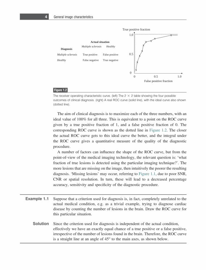
One familiar example of spatial frequencies is a standard optician’s test. In one test,patients are asked to look at a series of black lines on a white background, and thento tell the optician if they can resolve the lines when a series of lenses with differentstrengths are used. As shown in Figure 1.3, the lines are of different thickness andseparation. The spatial frequency of a particular grid of lines is measured asthe number of lines/mm, for example 5 mm21 for lines spaced 200 lm apart. Thecloser together are the lines, the higher is the spatial frequency, and the better thespatial resolution of the image system needs to be to resolve each individual line.
For each medical imaging modality, a number of factors affect the resolvingpower. One can simplify the analysis by considering just two general components:first the instrumentation used to form the image, and second the quantity of datathat is acquired i.e. the image data matrix size. To take the everyday example of adigital camera, the lens and electronics associated with the charge-coupled device(CCD) detector form the instrumentation, and the number of pixels (megapixels) ofthe camera dictates the amount of data that is acquired. The relative contribution ofeach component to the overall spatial resolution is important in an optimal
a b c
Figure 1.3
Grid patterns with increasing spatial frequencies going from (a) to (c).
5 1.3 Spatial resolution
engineering design. There is no advantage in terms of image quality in increasingthe CCD matrix size from 10 megapixels to 20 megapixels if the characteristics ofthe lens are poor, e.g. it is not well focused, produces blur, or has chromaticaberration. Similarly, if the lens is extremely well-made, then it would be sub-optimal to have a CCD with only 1 megapixel capability, and image quality wouldbe improved by being able to acquire a much greater number of pixels.
1.3.2 The line spread function
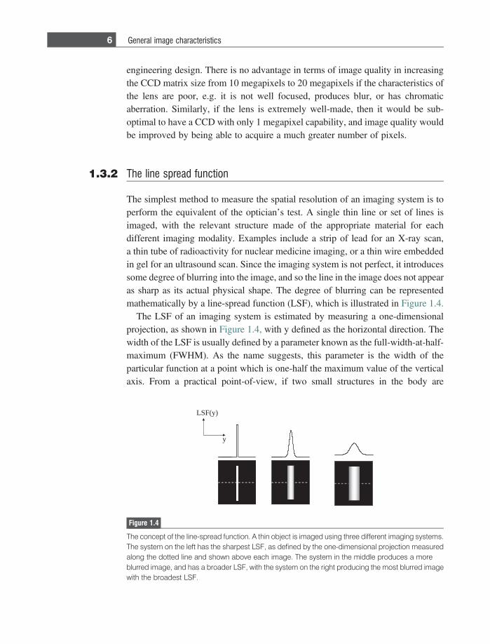
The simplest method to measure the spatial resolution of an imaging system is toperform the equivalent of the optician’s test. A single thin line or set of lines isimaged, with the relevant structure made of the appropriate material for eachdifferent imaging modality. Examples include a strip of lead for an X-ray scan,a thin tube of radioactivity for nuclear medicine imaging, or a thin wire embeddedin gel for an ultrasound scan. Since the imaging system is not perfect, it introducessome degree of blurring into the image, and so the line in the image does not appearas sharp as its actual physical shape. The degree of blurring can be representedmathematically by a line-spread function (LSF), which is illustrated in Figure 1.4.
The LSF of an imaging system is estimated by measuring a one-dimensionalprojection, as shown in Figure 1.4, with y defined as the horizontal direction. Thewidth of the LSF is usually defined by a parameter known as the full-width-at-half-maximum (FWHM). As the name suggests, this parameter is the width of theparticular function at a point which is one-half the maximum value of the verticalaxis. From a practical point-of-view, if two small structures in the body are
LSF(y)
y
Figure 1.4
The concept of the line-spread function. A thin object is imaged using three different imaging systems.The system on the left has the sharpest LSF, as defined by the one-dimensional projection measuredalong the dotted line and shown above each image. The system in the middle produces a moreblurred image, and has a broader LSF, with the system on the right producing the most blurred imagewith the broadest LSF.
6 General image characteristics
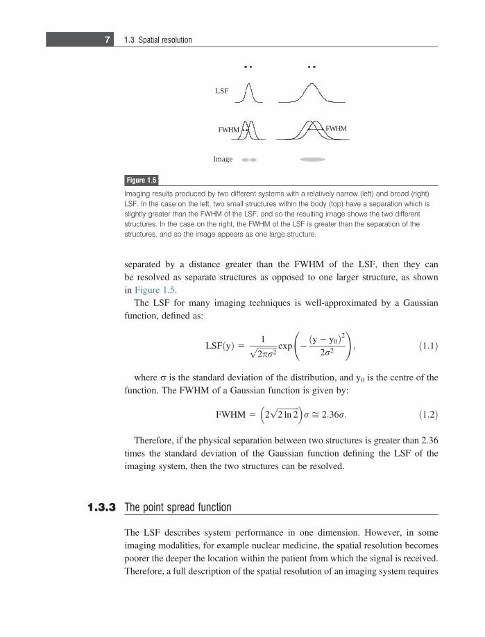
separated by a distance greater than the FWHM of the LSF, then they canbe resolved as separate structures as opposed to one larger structure, as shownin Figure 1.5.
The LSF for many imaging techniques is well-approximated by a Gaussianfunction, defined as:
LSF yð Þ 51ffiffiffiffiffiffiffiffiffiffi
2pr2p exp � y� y0ð Þ2
2r2
!; ð1:1Þ
where r is the standard deviation of the distribution, and y0 is the centre of thefunction. The FWHM of a Gaussian function is given by:
FWHM 5 2ffiffiffiffiffiffiffiffiffiffiffi2 ln 2p� �
r ffi 2:36r: ð1:2Þ
Therefore, if the physical separation between two structures is greater than 2.36times the standard deviation of the Gaussian function defining the LSF of theimaging system, then the two structures can be resolved.
1.3.3 The point spread function
The LSF describes system performance in one dimension. However, in someimaging modalities, for example nuclear medicine, the spatial resolution becomespoorer the deeper the location within the patient from which the signal is received.Therefore, a full description of the spatial resolution of an imaging system requires
MHWF MHWF
FSL
egamI
Figure 1.5
Imaging results produced by two different systems with a relatively narrow (left) and broad (right)LSF. In the case on the left, two small structures within the body (top) have a separation which isslightly greater than the FWHM of the LSF, and so the resulting image shows the two differentstructures. In the case on the right, the FWHM of the LSF is greater than the separation of thestructures, and so the image appears as one large structure.
7 1.3 Spatial resolution
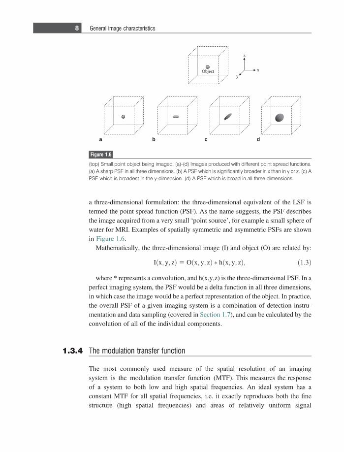
a three-dimensional formulation: the three-dimensional equivalent of the LSF istermed the point spread function (PSF). As the name suggests, the PSF describesthe image acquired from a very small ‘point source’, for example a small sphere ofwater for MRI. Examples of spatially symmetric and asymmetric PSFs are shownin Figure 1.6.
Mathematically, the three-dimensional image (I) and object (O) are related by:
I x; y; zð Þ 5 O x; y; zð Þ � h x; y; zð Þ; ð1:3Þ
where * represents a convolution, and h(x,y,z) is the three-dimensional PSF. In aperfect imaging system, the PSF would be a delta function in all three dimensions,in which case the image would be a perfect representation of the object. In practice,the overall PSF of a given imaging system is a combination of detection instru-mentation and data sampling (covered in Section 1.7), and can be calculated by theconvolution of all of the individual components.
1.3.4 The modulation transfer function
The most commonly used measure of the spatial resolution of an imagingsystem is the modulation transfer function (MTF). This measures the responseof a system to both low and high spatial frequencies. An ideal system has aconstant MTF for all spatial frequencies, i.e. it exactly reproduces both the finestructure (high spatial frequencies) and areas of relatively uniform signal
Object x
y
z
a b c d
Figure 1.6
(top) Small point object being imaged. (a)-(d) Images produced with different point spread functions.(a) A sharp PSF in all three dimensions. (b) A PSF which is significantly broader in x than in y or z. (c) APSF which is broadest in the y-dimension. (d) A PSF which is broad in all three dimensions.
8 General image characteristics
intensity (low spatial frequencies). In practice, as seen previously, imagingsystems have a finite spatial resolution, and the high spatial frequencies mustat some value start to be attenuated: the greater the attenuation the poorer thespatial resolution. Mathematically, the MTF is given by the Fourier transform ofthe PSF:
MTF kx; ky; kz� �
5 F PSF x; y; zð Þf g; ð1:4Þ
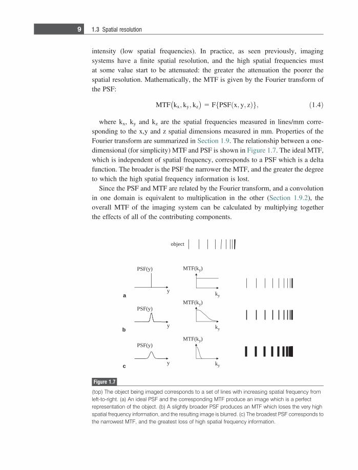
where kx, ky and kz are the spatial frequencies measured in lines/mm corre-sponding to the x,y and z spatial dimensions measured in mm. Properties of theFourier transform are summarized in Section 1.9. The relationship between a one-dimensional (for simplicity) MTF and PSF is shown in Figure 1.7. The ideal MTF,which is independent of spatial frequency, corresponds to a PSF which is a deltafunction. The broader is the PSF the narrower the MTF, and the greater the degreeto which the high spatial frequency information is lost.
Since the PSF and MTF are related by the Fourier transform, and a convolutionin one domain is equivalent to multiplication in the other (Section 1.9.2), theoverall MTF of the imaging system can be calculated by multiplying togetherthe effects of all of the contributing components.
k(FTM y)
ky
ky
ky
)y(FSP
y
y
y
)y(FSP
)y(FSP
k(FTM y)
k(FTM y)
tcejbo
a
b
c
Figure 1.7
(top) The object being imaged corresponds to a set of lines with increasing spatial frequency fromleft-to-right. (a) An ideal PSF and the corresponding MTF produce an image which is a perfectrepresentation of the object. (b) A slightly broader PSF produces an MTF which loses the very highspatial frequency information, and the resulting image is blurred. (c) The broadest PSF corresponds tothe narrowest MTF, and the greatest loss of high spatial frequency information.
9 1.3 Spatial resolution
1.4 Signal-to-noise ratio
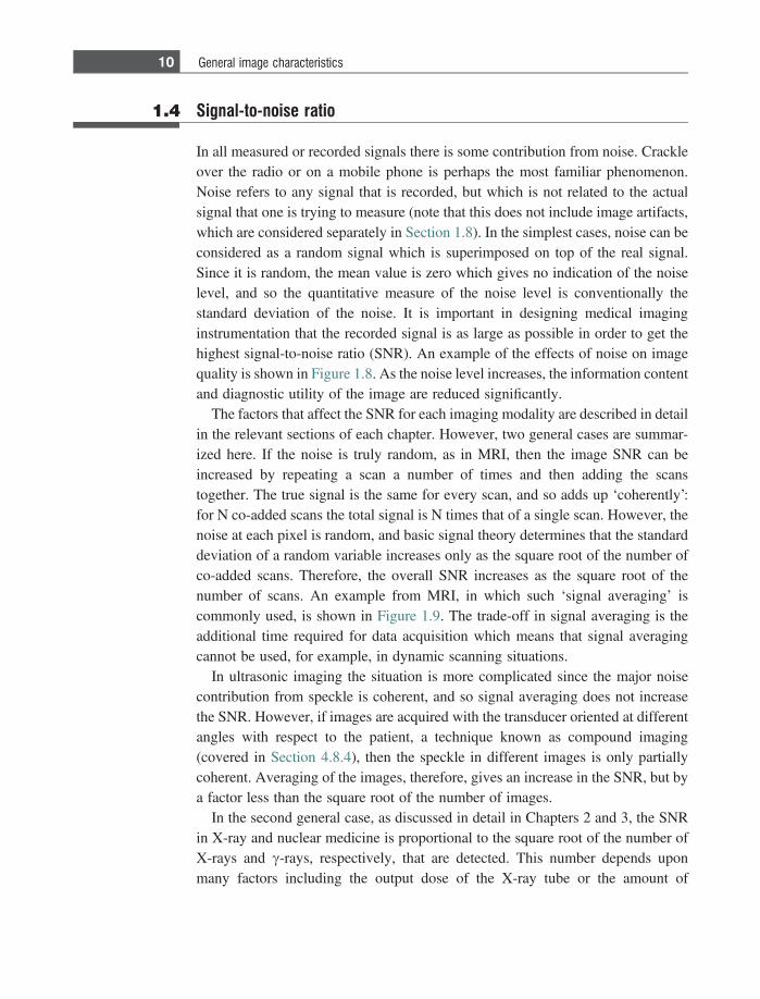
In all measured or recorded signals there is some contribution from noise. Crackleover the radio or on a mobile phone is perhaps the most familiar phenomenon.Noise refers to any signal that is recorded, but which is not related to the actualsignal that one is trying to measure (note that this does not include image artifacts,which are considered separately in Section 1.8). In the simplest cases, noise can beconsidered as a random signal which is superimposed on top of the real signal.Since it is random, the mean value is zero which gives no indication of the noiselevel, and so the quantitative measure of the noise level is conventionally thestandard deviation of the noise. It is important in designing medical imaginginstrumentation that the recorded signal is as large as possible in order to get thehighest signal-to-noise ratio (SNR). An example of the effects of noise on imagequality is shown in Figure 1.8. As the noise level increases, the information contentand diagnostic utility of the image are reduced significantly.
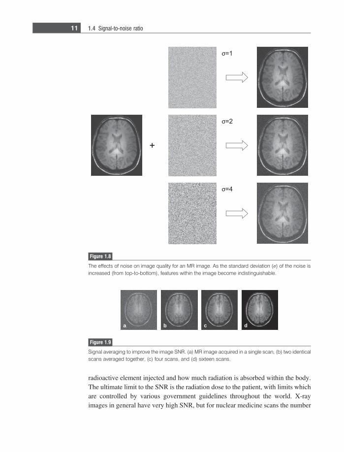
The factors that affect the SNR for each imaging modality are described in detailin the relevant sections of each chapter. However, two general cases are summar-ized here. If the noise is truly random, as in MRI, then the image SNR can beincreased by repeating a scan a number of times and then adding the scanstogether. The true signal is the same for every scan, and so adds up ‘coherently’:for N co-added scans the total signal is N times that of a single scan. However, thenoise at each pixel is random, and basic signal theory determines that the standarddeviation of a random variable increases only as the square root of the number ofco-added scans. Therefore, the overall SNR increases as the square root of thenumber of scans. An example from MRI, in which such ‘signal averaging’ iscommonly used, is shown in Figure 1.9. The trade-off in signal averaging is theadditional time required for data acquisition which means that signal averagingcannot be used, for example, in dynamic scanning situations.
In ultrasonic imaging the situation is more complicated since the major noisecontribution from speckle is coherent, and so signal averaging does not increasethe SNR. However, if images are acquired with the transducer oriented at differentangles with respect to the patient, a technique known as compound imaging(covered in Section 4.8.4), then the speckle in different images is only partiallycoherent. Averaging of the images, therefore, gives an increase in the SNR, but bya factor less than the square root of the number of images.
In the second general case, as discussed in detail in Chapters 2 and 3, the SNRin X-ray and nuclear medicine is proportional to the square root of the number ofX-rays and c-rays, respectively, that are detected. This number depends uponmany factors including the output dose of the X-ray tube or the amount of
10 General image characteristics
radioactive element injected and how much radiation is absorbed within the body.The ultimate limit to the SNR is the radiation dose to the patient, with limits whichare controlled by various government guidelines throughout the world. X-rayimages in general have very high SNR, but for nuclear medicine scans the number
a b c d
Figure 1.9
Signal averaging to improve the image SNR. (a) MR image acquired in a single scan, (b) two identicalscans averaged together, (c) four scans, and (d) sixteen scans.
Figure 1.8
The effects of noise on image quality for an MR image. As the standard deviation (r) of the noise isincreased (from top-to-bottom), features within the image become indistinguishable.
11 1.4 Signal-to-noise ratio
of c-rays detected is much lower, and so the scanning time is prolonged comparedto X-ray scans, with the total time limited by patient comfort.
1.5 Contrast-to-noise ratio
Even if a particular image has a very high SNR, it is not diagnostically usefulunless there is a high enough CNR to be able to distinguish between differenttissues, and in particular between healthy and pathological tissue. Various defini-tions of image contrast exist, the most common being:
CAB 5 SA � SBj j; ð1:5Þ
where CAB is the contrast between tissues A and B, and SA and SB are the signalsfrom tissues A and B, respectively. The CNR between tissues A and B is defined interms of the respective SNRs of the two tissues:
CNRAB 5CAB
rN5
SA � SBj jrN
5 SNRA � SNRBj j; ð1:6Þ
where rN is the standard deviation of the noise.In addition to the intrinsic contrast between particular tissues, the CNR clearly
depends both on the image SNR and spatial resolution. For example, in Figure 1.1,a decreased spatial resolution in Figure 1.1(b) reduced the image CNR due to‘partial volume’ effects. This means that the contrast between the lesion andhealthy tissue is decreased, since voxels (volumetric pixels) contain contributionsfrom both the high contrast lesion, but also from the surrounding tissue due to thebroadened PSF. Figure 1.1(c) and Equation (1.6) show that a reduced SNR alsoreduces the CNR.
1.6 Image filtering
After the data have been acquired and digitized and the images reconstructed,further enhancements can be made by filtering the images. This process is similarto that available in many software products for digital photography. The particularfilter used depends upon the imaging modality, and the image characteristics thatmost need to be enhanced.
The simplest types of filter are either high-pass or low-pass, referring to theircharacteristics in the spatial frequency domain, i.e. a high-pass filter accentuatesthe high spatial frequency components in the image, and vice-versa. High spatial
12 General image characteristics
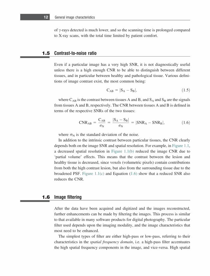
frequencies correspond to small objects and edges in the images, and so these are‘sharpened’ using a high-pass filter, therefore improving the spatial resolution.However, the noise present in the image, since it has a random pixel-to-pixelvariation, also corresponds to very high spatial frequencies, and so the SNR of ahigh-pass filtered image decreases, as shown in Figure 1.10. A high-pass filter issuited, therefore, to images with very high intrinsic SNR, in which the aim is tomake out very fine details.
In contrast, a low-pass filter attenuates the noise, therefore increasing the SNRin the filtered image. The trade-off is that other features in the image which arealso represented by high spatial frequencies, e.g. small features, are smoothed outby this type of filter. Low-pass filters are typically applied to images with intrinsi-cally low SNR and relatively poor spatial resolution (which is not substantiallyfurther degraded by application of the filter), such as planar nuclear medicinescans.
Specialized filters can also be used for detecting edges in images, for example.This process is very useful if the aim is to segment images into different tissuecompartments. Since edges have a steep gradient in signal intensity from one pixelto the adjacent one, one can consider the basic approach to be measuring the slope
k
Low-pass filter
MTF(k)
k
High-pass filter
MTF(k)
Figure 1.10
The effects of low-pass and high-pass filtering. Low-pass filters improve the SNR at the expense of aloss in spatial resolution: high-pass filters increase the spatial resolution but reduce the SNR.
13 1.6 Image filtering
of the image by performing a spatial derivative. Since edge detection also amplifiesthe noise in an image, the process is usually followed by some form of low-passfiltering to reduce the noise.
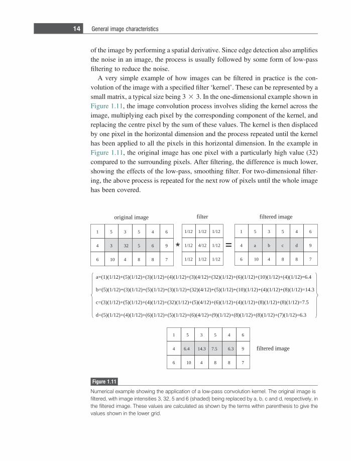
A very simple example of how images can be filtered in practice is the con-volution of the image with a specified filter ‘kernel’. These can be represented by asmall matrix, a typical size being 3 3 3. In the one-dimensional example shown inFigure 1.11, the image convolution process involves sliding the kernel across theimage, multiplying each pixel by the corresponding component of the kernel, andreplacing the centre pixel by the sum of these values. The kernel is then displacedby one pixel in the horizontal dimension and the process repeated until the kernelhas been applied to all the pixels in this horizontal dimension. In the example inFigure 1.11, the original image has one pixel with a particularly high value (32)compared to the surrounding pixels. After filtering, the difference is much lower,showing the effects of the low-pass, smoothing filter. For two-dimensional filter-ing, the above process is repeated for the next row of pixels until the whole imagehas been covered.
351
2334
4016
645
965
788
21/121/121/1
21/121/421/1
21/121/121/1
351
ba4
4016
645
9dc
788
/4()3(+)21/1()4(+)21/1()3(+)21/1()5(+)21/1()1(=a 4.6=)21/1()4(+)21/1()01(+)21/1()6(+)21/1()23(+)21
/4()23(+)21/1()3(+)21/1()5(+)21/1()3(+)21/1()5(=b 3.41=)21/1()8(+)21/1()4(+)21/1()01(+)21/1()5(+)21
/4()5(+)21/1()23(+)21/1()4(+)21/1()5(+)21/1()3(=c 5.7=)21/1()8(+)21/1()8(+)21/1()4(+)21/1()6(+)21
/4()6(+)21/1()5(+)21/1()6(+)21/1()4(+)21/1()5(=d 3.6=)21/1()7(+)21/1()8(+)21/1()8(+)21/1()9(+)21
351
3.414.64
4016
645
96.35.7
788
egami lanigiro retlif egami deretlif
egami deretlif
Figure 1.11
Numerical example showing the application of a low-pass convolution kernel. The original image isfiltered, with image intensities 3, 32, 5 and 6 (shaded) being replaced by a, b, c and d, respectively, inthe filtered image. These values are calculated as shown by the terms within parenthesis to give thevalues shown in the lower grid.
14 General image characteristics
This is a very simple demonstration of filtering. In practice much more sophis-ticated mathematical approaches can be used to optimize the performance of thefilter given the properties of the particular image. This is especially true if the MTFof the system is known, in which case either ‘matched’ filtering or deconvolutiontechniques can be used.
1.7 Data acquisition: analogue-to-digital converters
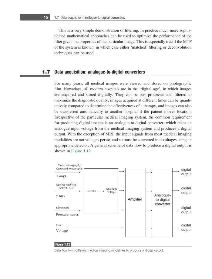
For many years, all medical images were viewed and stored on photographicfilm. Nowadays, all modern hospitals are in the ‘digital age’, in which imagesare acquired and stored digitally. They can be post-processed and filtered tomaximize the diagnostic quality, images acquired at different times can be quanti-tatively compared to determine the effectiveness of a therapy, and images can alsobe transferred automatically to another hospital if the patient moves location.Irrespective of the particular medical imaging system, the common requirementfor producing digital images is an analogue-to-digital converter, which takes ananalogue input voltage from the medical imaging system and produces a digitaloutput. With the exception of MRI, the input signals from most medical imagingmodalities are not voltages per se, and so must be converted into voltages using anappropriate detector. A general scheme of data flow to produce a digital output isshown in Figure 1.12.
X-rays
Planar radiographyComputed tomography
-rays
Nuclear medicineSPECT, PET
Pressure waves
Ultrasound
Voltage
MRI
Detector
Analogue-to-digitalconverter
digitaloutput
digitaloutput
digitaloutput
digitaloutput
Amplifier
Analoguevoltage
Figure 1.12
Data flow from different medical imaging modalities to produce a digital output.
15 1.7 Data acquisition: analogue-to-digital converters
1.7.1 Dynamic range and resolution
The ideal analogue-to-digital converter (ADC) converts a continuous voltage sig-nal into a digital signal with as high a fidelity as possible, while introducing as littlenoise as possible. The important specifications of an ADC are the dynamic range,voltage range (maximum-to-minimum), maximum sampling frequency and fre-quency bandwidth.
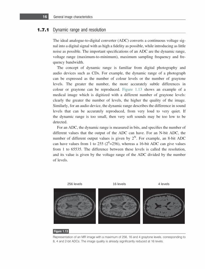
The concept of dynamic range is familiar from digital photography andaudio devices such as CDs. For example, the dynamic range of a photographcan be expressed as the number of colour levels or the number of graytonelevels. The greater the number, the more accurately subtle differences incolour or graytone can be reproduced. Figure 1.13 shows an example of amedical image which is digitized with a different number of graytone levels:clearly the greater the number of levels, the higher the quality of the image.Similarly, for an audio device, the dynamic range describes the difference in soundlevels that can be accurately reproduced, from very loud to very quiet. Ifthe dynamic range is too small, then very soft sounds may be too low to bedetected.
For an ADC, the dynamic range is measured in bits, and specifies the number ofdifferent values that the output of the ADC can have. For an N-bit ADC, thenumber of different output values is given by 2N. For example, an 8-bit ADCcan have values from 1 to 255 (28=256), whereas a 16-bit ADC can give valuesfrom 1 to 65535. The difference between these levels is called the resolution,and its value is given by the voltage range of the ADC divided by the numberof levels.
256 levels 16 levels 4 levels
Figure 1.13
Representation of an MR image with a maximum of 256, 16 and 4 graytone levels, corresponding to8, 4 and 2-bit ADCs. The image quality is already significantly reduced at 16 levels.
16 General image characteristics
Example 1.2 What is the minimum voltage difference that can be measured by a 5 volt, 12-bitADC?
Solution There are 4096 different levels that can be measured by the ADC, with values from25 to 5 volts (note that the maximum voltage of the ADC refers to positive andnegative values). Therefore, the minimum voltage difference is given by 10/4096 =2.44 mV.
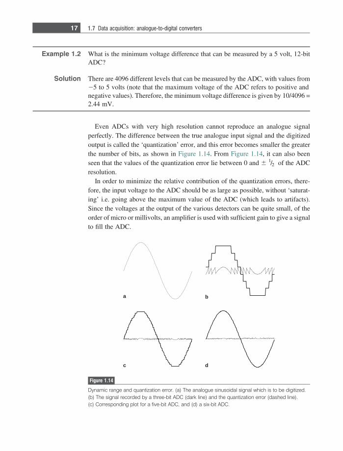
Even ADCs with very high resolution cannot reproduce an analogue signalperfectly. The difference between the true analogue input signal and the digitizedoutput is called the ‘quantization’ error, and this error becomes smaller the greaterthe number of bits, as shown in Figure 1.14. From Figure 1.14, it can also beenseen that the values of the quantization error lie between 0 and 6 1/2 of the ADCresolution.
In order to minimize the relative contribution of the quantization errors, there-fore, the input voltage to the ADC should be as large as possible, without ‘saturat-ing’ i.e. going above the maximum value of the ADC (which leads to artifacts).Since the voltages at the output of the various detectors can be quite small, of theorder of micro or millivolts, an amplifier is used with sufficient gain to give a signalto fill the ADC.
a b
c d
Figure 1.14
Dynamic range and quantization error. (a) The analogue sinusoidal signal which is to be digitized.(b) The signal recorded by a three-bit ADC (dark line) and the quantization error (dashed line).(c) Corresponding plot for a five-bit ADC, and (d) a six-bit ADC.
17 1.7 Data acquisition: analogue-to-digital converters
1.7.2 Sampling frequency and bandwidth
The second important set of specifications for the ADC is the maximumfrequency that can be sampled and the bandwidth over which measurementsare to be made. The Nyquist theorem states that a signal must be sampled at leasttwice as fast as the bandwidth of the signal to reconstruct the waveform accurately,otherwise the high-frequency content will alias at a frequency inside the spectrumof interest [1;2].
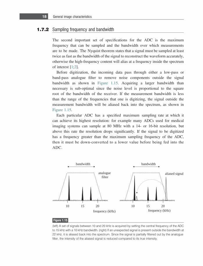
Before digitization, the incoming data pass through either a low-pass orband-pass analogue filter to remove noise components outside the signalbandwidth as shown in Figure 1.15. Acquiring a larger bandwidth thannecessary is sub-optimal since the noise level is proportional to the squareroot of the bandwidth of the receiver. If the measurement bandwidth is lessthan the range of the frequencies that one is digitizing, the signal outside themeasurement bandwidth will be aliased back into the spectrum, as shown inFigure 1.15.
Each particular ADC has a specified maximum sampling rate at which itcan achieve its highest resolution: for example many ADCs used for medicalimaging systems can sample at 80 MHz with a 14- or 16-bit resolution, butabove this rate the resolution drops significantly. If the signal to be digitizedhas a frequency greater than the maximum sampling frequency of the ADC,then it must be down-converted to a lower value before being fed into theADC.
51 0201
langis desaila
htdiwdnab
)zHk( ycneuqerf51 0201
htdiwdnab
)zHk( ycneuqerf
eugolanaretlif
Figure 1.15
(left) A set of signals between 10 and 20 kHz is acquired by setting the central frequency of the ADCto 15 kHz with a 10 kHz bandwidth. (right) If an unexpected signal is present outside the bandwidth at22 kHz, it is aliased back into the spectrum. Since the signal is partially filtered out by the analoguefilter, the intensity of the aliased signal is reduced compared to its true intensity.
18 General image characteristics
1.7.3 Digital oversampling
There are a number of problems with the simple sampling scheme described in theprevious section. First, the analogue filters cannot be made absolutely ‘sharp’ (andhave other problems such as group delays and frequency-dependent phase shiftsthat are not discussed here). Second, the resolution of a 14- or 16-bit ADC may notbe sufficient to avoid quantization noise, but higher resolution ADCs typically donot have high enough sampling rates and are extremely expensive. Fortunately,there is a method, termed oversampling, which can alleviate both issues [3].
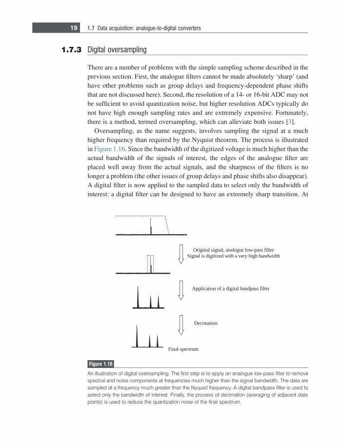
Oversampling, as the name suggests, involves sampling the signal at a muchhigher frequency than required by the Nyquist theorem. The process is illustratedin Figure 1.16. Since the bandwidth of the digitized voltage is much higher than theactual bandwidth of the signals of interest, the edges of the analogue filter areplaced well away from the actual signals, and the sharpness of the filters is nolonger a problem (the other issues of group delays and phase shifts also disappear).A digital filter is now applied to the sampled data to select only the bandwidth ofinterest: a digital filter can be designed to have an extremely sharp transition. At
retlif ssap-wol eugolana ,langis lanigirOhtdiwdnab hgih yrev a htiw dezitigid si langiS
retlifssapdnab latigid a fo noitacilppA
noitamiceD
murtceps laniF
Figure 1.16
An illustration of digital oversampling. The first step is to apply an analogue low-pass filter to removespectral and noise components at frequencies much higher than the signal bandwidth. The data aresampled at a frequency much greater than the Nyquist frequency. A digital bandpass filter is used toselect only the bandwidth of interest. Finally, the process of decimation (averaging of adjacent datapoints) is used to reduce the quantization noise of the final spectrum.
19 1.7 Data acquisition: analogue-to-digital converters
this stage, the filtered data have N-times as many data points (where N is theoversampling factor) as would have been acquired without oversampling, andthe final step is to ‘decimate’ the data, in which successive data points are averagedtogether. Since the quantization error in alternate data points is assumed to berandom, the quantization noise in the decimated data set is reduced. For everyfactor-of-four in oversampling, the equivalent resolution of the ADC increases by1-bit.
1.8 Image artifacts
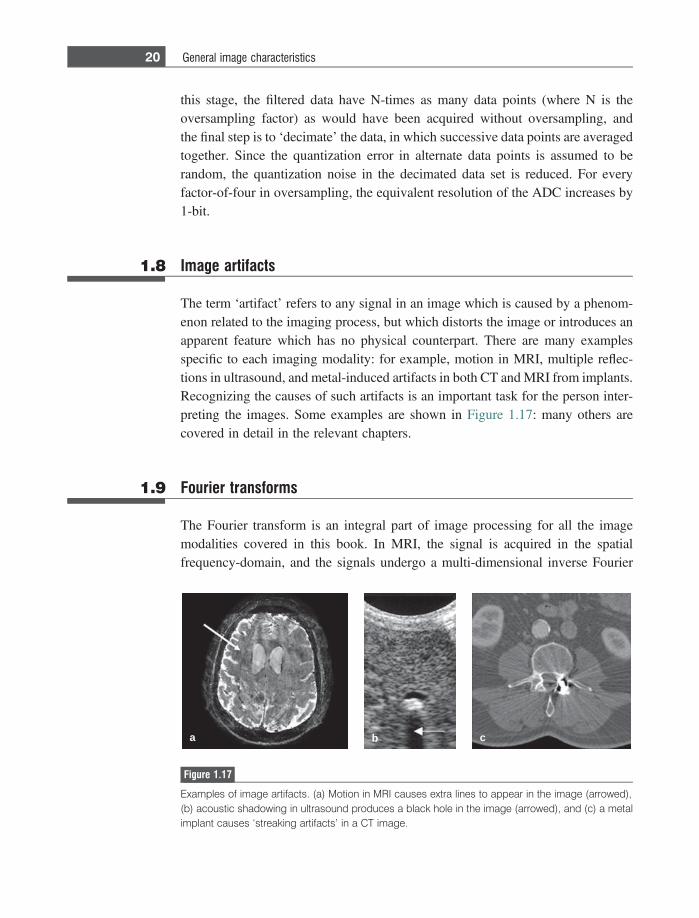
The term ‘artifact’ refers to any signal in an image which is caused by a phenom-enon related to the imaging process, but which distorts the image or introduces anapparent feature which has no physical counterpart. There are many examplesspecific to each imaging modality: for example, motion in MRI, multiple reflec-tions in ultrasound, and metal-induced artifacts in both CT and MRI from implants.Recognizing the causes of such artifacts is an important task for the person inter-preting the images. Some examples are shown in Figure 1.17: many others arecovered in detail in the relevant chapters.
1.9 Fourier transforms
The Fourier transform is an integral part of image processing for all the imagemodalities covered in this book. In MRI, the signal is acquired in the spatialfrequency-domain, and the signals undergo a multi-dimensional inverse Fourier
a b c
Figure 1.17
Examples of image artifacts. (a) Motion in MRI causes extra lines to appear in the image (arrowed),(b) acoustic shadowing in ultrasound produces a black hole in the image (arrowed), and (c) a metalimplant causes ‘streaking artifacts’ in a CT image.
20 General image characteristics
transform to produce the image. In CT, SPECT and PET, filtered backprojectionalgorithms are implemented using Fourier transforms. In ultrasonic imaging, spec-tral Doppler plots are the result of Fourier transformation of the time-domaindemodulated Doppler signals. This section summarizes the basis mathematicsand properties of the Fourier transform, with emphasis on those properties relevantto the imaging modalities covered.
1.9.1 Fourier transformation of time- and spatialfrequency-domain signals
The forward Fourier transform of a time-domain signal, s(t), is given by:
SðfÞ 5
�
sðtÞe�j2pftdt: ð1:7Þ
The inverse Fourier transform of a frequency-domain signal, S(f), is given by:
sðtÞ 51
2p
�
SðfÞe1 j2pftdf: ð1:8Þ
The forward Fourier transform of a spatial-domain signal, q(x), has the form:
SðkÞ 5
�
sðxÞe�j2pkxxdx: ð1:9Þ
The corresponding inverse Fourier transform of a spatial frequency-domainsignal, S(k), is given by:
sðxÞ 5
�
SðkÞe1 j2pkxxdk: ð1:10Þ
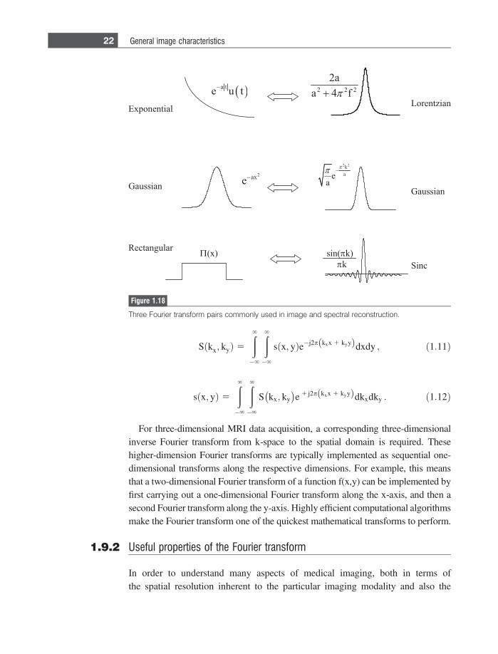
Some useful Fourier-pairs are shown in Figure 1.18: each of the particularfunctions occurs in multiple instances in the medical imaging modalities coveredhere.
In imaging, signals are clearly often acquired in more than one dimension, andimage reconstruction then requires multi-dimensional Fourier transformation. Forexample, MRI intrinsically acquires two-dimensional k-space data, for which theFourier pairs are given by:
21 1.9 Fourier transforms
Sðkx; kyÞ 5
�
�
sðx; yÞe�j2p kxx 1 kyyð Þdxdy ; ð1:11Þ
sðx; yÞ 5
�
�
S kx; ky� �
e 1 j2p kxx 1 kyyð Þdkxdky : ð1:12Þ
For three-dimensional MRI data acquisition, a corresponding three-dimensionalinverse Fourier transform from k-space to the spatial domain is required. Thesehigher-dimension Fourier transforms are typically implemented as sequential one-dimensional transforms along the respective dimensions. For example, this meansthat a two-dimensional Fourier transform of a function f(x,y) can be implemented byfirst carrying out a one-dimensional Fourier transform along the x-axis, and then asecond Fourier transform along the y-axis. Highly efficient computational algorithmsmake the Fourier transform one of the quickest mathematical transforms to perform.
1.9.2 Useful properties of the Fourier transform
In order to understand many aspects of medical imaging, both in terms ofthe spatial resolution inherent to the particular imaging modality and also the
Figure 1.18
Three Fourier transform pairs commonly used in image and spectral reconstruction.
22 General image characteristics

effects of image post-processing, a number of mathematical properties of theFourier transform are very useful. The most relevant examples are listed below,with specific examples from the imaging modalities covered in this book.
(a) Linearity. The Fourier transform of two additive functions is additive:
as1ðtÞ 1 bs2ðtÞ5aS1ðfÞ 1 bS2ðfÞ ,aS1ðxÞ 1 bS2ðxÞ5as1ðkxÞ 1 bs2ðkxÞ
ð1:13Þ
where 5 represents forward Fourier transformation from left-to-right, and theinverse Fourier transform from right-to-left. This theorem shows that when theacquired signal is, for example, the sum of a number of different sinusoidalfunctions, each with a different frequency and different amplitude, then therelative amplitudes of these components are maintained when the data areFourier transformed, as shown in Figure 1.19.
(b) Convolution. If two signals are multiplied together, then the signal in theFourier domain is given by the convolution of the two individual Fouriertransformed components, e.g.
s1 tð Þs2 tð Þ5S1 fð Þ � S2 fð Þ ,s1 kxð Þs2 kxð Þ5S1 xð Þ � S2 xð Þ
ð1:14Þ
where * represents a convolution. This relationship is shown in Figure 1.20.The convolution, f(x), of two functions p(x) and q(x) is defined as:
f xð Þ 5 p xð Þ � q xð Þ 5
�
p x� sð Þq sð Þds: ð1:15Þ
emit
ycneuqerf
+
+
emit
TF
f1
f1
f2 f3
f2
f3
=
Figure 1.19
A time-domain signal (centre) is composed of three different time-domain signals (left). The Fouriertransformed frequency spectrum (right) produces signals for each of the three frequencies with thesame amplitudes as in the time-domain data.
23 1.9 Fourier transforms
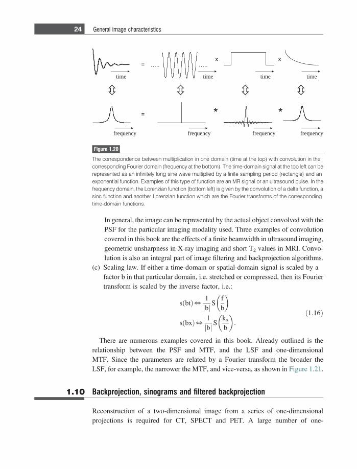
In general, the image can be represented by the actual object convolved with thePSF for the particular imaging modality used. Three examples of convolutioncovered in this book are the effects of a finite beamwidth in ultrasound imaging,geometric unsharpness in X-ray imaging and short T2 values in MRI. Convo-lution is also an integral part of image filtering and backprojection algorithms.
(c) Scaling law. If either a time-domain or spatial-domain signal is scaled by afactor b in that particular domain, i.e. stretched or compressed, then its Fouriertransform is scaled by the inverse factor, i.e.:
sðbtÞ5 1bj j S
fb
� �
sðbxÞ5 1bj j S
kx
b
� �:
ð1:16Þ
There are numerous examples covered in this book. Already outlined is therelationship between the PSF and MTF, and the LSF and one-dimensionalMTF. Since the parameters are related by a Fourier transform the broader theLSF, for example, the narrower the MTF, and vice-versa, as shown in Figure 1.21.
1.10 Backprojection, sinograms and filtered backprojection
Reconstruction of a two-dimensional image from a series of one-dimensionalprojections is required for CT, SPECT and PET. A large number of one-
…..…..
frequency
time
frequency frequency frequency
time time time
Figure 1.20
The correspondence between multiplication in one domain (time at the top) with convolution in thecorresponding Fourier domain (frequency at the bottom). The time-domain signal at the top left can berepresented as an infinitely long sine wave multiplied by a finite sampling period (rectangle) and anexponential function. Examples of this type of function are an MR signal or an ultrasound pulse. In thefrequency domain, the Lorenzian function (bottom left) is given by the convolution of a delta function, asinc function and another Lorenzian function which are the Fourier transforms of the correspondingtime-domain functions.
24 General image characteristics
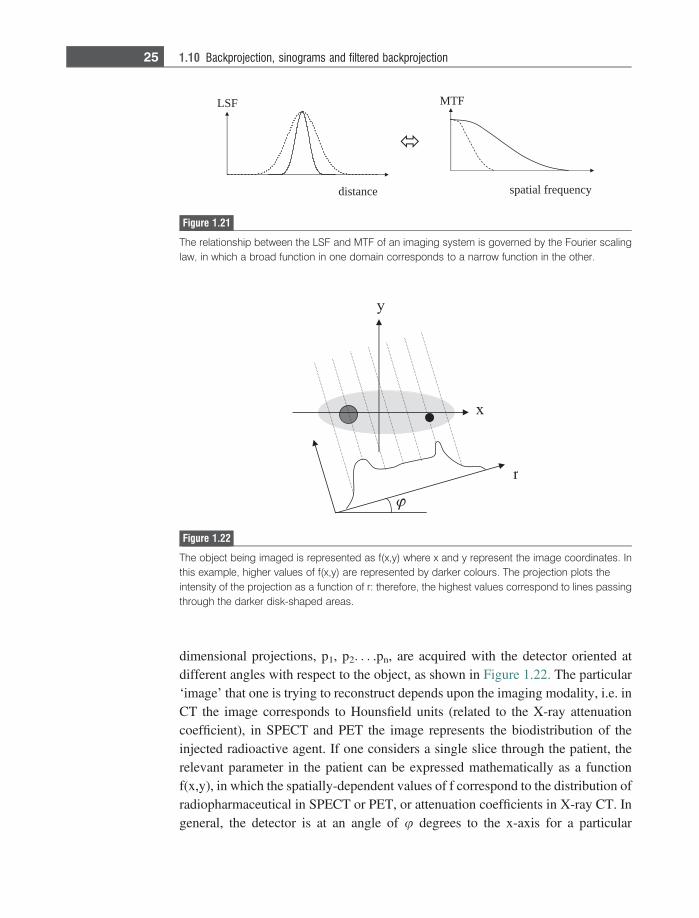
dimensional projections, p1, p2. . . .pn, are acquired with the detector oriented atdifferent angles with respect to the object, as shown in Figure 1.22. The particular‘image’ that one is trying to reconstruct depends upon the imaging modality, i.e. inCT the image corresponds to Hounsfield units (related to the X-ray attenuationcoefficient), in SPECT and PET the image represents the biodistribution of theinjected radioactive agent. If one considers a single slice through the patient, therelevant parameter in the patient can be expressed mathematically as a functionf(x,y), in which the spatially-dependent values of f correspond to the distribution ofradiopharmaceutical in SPECT or PET, or attenuation coefficients in X-ray CT. Ingeneral, the detector is at an angle of u degrees to the x-axis for a particular
MTF
spatial frequency
LSF
distance
Figure 1.21
The relationship between the LSF and MTF of an imaging system is governed by the Fourier scalinglaw, in which a broad function in one domain corresponds to a narrow function in the other.
Figure 1.22
The object being imaged is represented as f(x,y) where x and y represent the image coordinates. Inthis example, higher values of f(x,y) are represented by darker colours. The projection plots theintensity of the projection as a function of r: therefore, the highest values correspond to lines passingthrough the darker disk-shaped areas.
25 1.10 Backprojection, sinograms and filtered backprojection
measurement, with u having values between 0 and 360�. The measured projectionat every angle u is denoted by p(r,u).
1.10.1 Backprojection
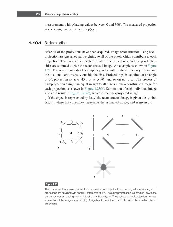
After all of the projections have been acquired, image reconstruction using back-projection assigns an equal weighting to all of the pixels which contribute to eachprojection. This process is repeated for all of the projections, and the pixel inten-sities are summed to give the reconstructed image. An example is shown in Figure1.23. The object consists of a simple cylinder with uniform intensity throughoutthe disk and zero intensity outside the disk. Projection p1 is acquired at an angleu=0�, projection p2 at u=45�, p3 at u=90� and so on up to p8. The process ofbackprojection assigns an equal weight to all pixels in the reconstructed image foreach projection, as shown in Figure 1.23(b). Summation of each individual imagegives the result in Figure 1.23(c), which is the backprojected image.
If the object is represented by f(x,y) the reconstructed image is given the symbolfðx; yÞ, where the circumflex represents the estimated image, and is given by:
p1 p2
p3
p4p5p6
p7
p8
1 2 3 4
5 6 7 8
c
a b
Figure 1.23
The process of backprojection. (a) From a small round object with uniform signal intensity, eightprojections are obtained with angular increments of 45�. The eight projections are shown in (b) with thedark areas corresponding to the highest signal intensity. (c) The process of backprojection involvessummation of the images shown in (b). A significant ‘star artifact’ is visible due to the small number ofprojections.
26 General image characteristics
fðx; yÞ 5 +n
j 5 1pðr;ujÞdu; ð1:17Þ
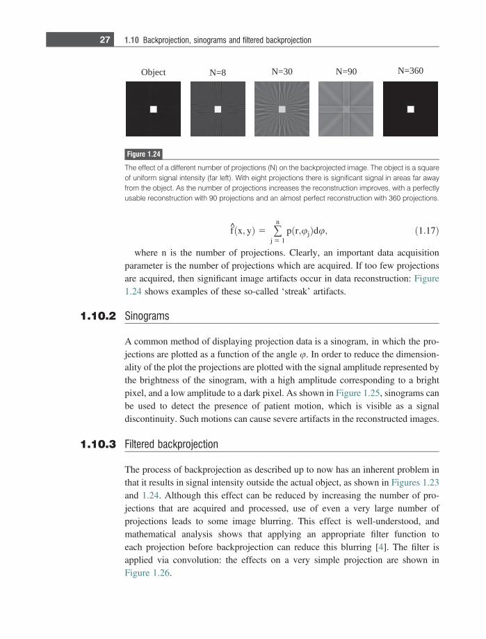
where n is the number of projections. Clearly, an important data acquisitionparameter is the number of projections which are acquired. If too few projectionsare acquired, then significant image artifacts occur in data reconstruction: Figure1.24 shows examples of these so-called ‘streak’ artifacts.
1.10.2 Sinograms
A common method of displaying projection data is a sinogram, in which the pro-jections are plotted as a function of the angle u. In order to reduce the dimension-ality of the plot the projections are plotted with the signal amplitude represented bythe brightness of the sinogram, with a high amplitude corresponding to a brightpixel, and a low amplitude to a dark pixel. As shown in Figure 1.25, sinograms canbe used to detect the presence of patient motion, which is visible as a signaldiscontinuity. Such motions can cause severe artifacts in the reconstructed images.
1.10.3 Filtered backprojection
The process of backprojection as described up to now has an inherent problem inthat it results in signal intensity outside the actual object, as shown in Figures 1.23and 1.24. Although this effect can be reduced by increasing the number of pro-jections that are acquired and processed, use of even a very large number ofprojections leads to some image blurring. This effect is well-understood, andmathematical analysis shows that applying an appropriate filter function toeach projection before backprojection can reduce this blurring [4]. The filter isapplied via convolution: the effects on a very simple projection are shown inFigure 1.26.
Object N=8 N=30 N=90 N=360
Figure 1.24
The effect of a different number of projections (N) on the backprojected image. The object is a squareof uniform signal intensity (far left). With eight projections there is significant signal in areas far awayfrom the object. As the number of projections increases the reconstruction improves, with a perfectlyusable reconstruction with 90 projections and an almost perfect reconstruction with 360 projections.
27 1.10 Backprojection, sinograms and filtered backprojection
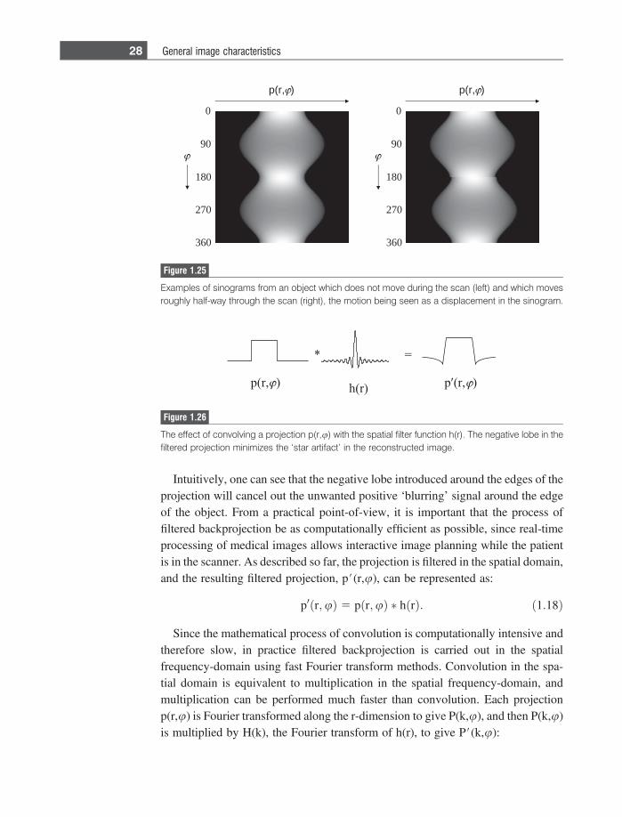
Intuitively, one can see that the negative lobe introduced around the edges of theprojection will cancel out the unwanted positive ‘blurring’ signal around the edgeof the object. From a practical point-of-view, it is important that the process offiltered backprojection be as computationally efficient as possible, since real-timeprocessing of medical images allows interactive image planning while the patientis in the scanner. As described so far, the projection is filtered in the spatial domain,and the resulting filtered projection, p#(r,u), can be represented as:
p0 r;uð Þ 5 p r;uð Þ � h rð Þ: ð1:18Þ
Since the mathematical process of convolution is computationally intensive andtherefore slow, in practice filtered backprojection is carried out in the spatialfrequency-domain using fast Fourier transform methods. Convolution in the spa-tial domain is equivalent to multiplication in the spatial frequency-domain, andmultiplication can be performed much faster than convolution. Each projectionp(r,u) is Fourier transformed along the r-dimension to give P(k,u), and then P(k,u)is multiplied by H(k), the Fourier transform of h(r), to give P#(k,u):
Figure 1.26
The effect of convolving a projection p(r,u) with the spatial filter function h(r). The negative lobe in thefiltered projection minimizes the ‘star artifact’ in the reconstructed image.
90
0
270
180
360
90
0
270
180
360
p(r, ) p(r, )
Figure 1.25
Examples of sinograms from an object which does not move during the scan (left) and which movesroughly half-way through the scan (right), the motion being seen as a displacement in the sinogram.
28 General image characteristics
P0 k;uð Þ 5 P k;uð ÞH kð Þ: ð1:19Þ
The filtered projections, P#(k,u), are inverse Fourier transformed back into thespatial-domain, and backprojected to give the final image, fðx; yÞ:
f x; yð Þ 5 +n
j 5 1F�1 P0 k;uj
� � du: ð1:20Þ
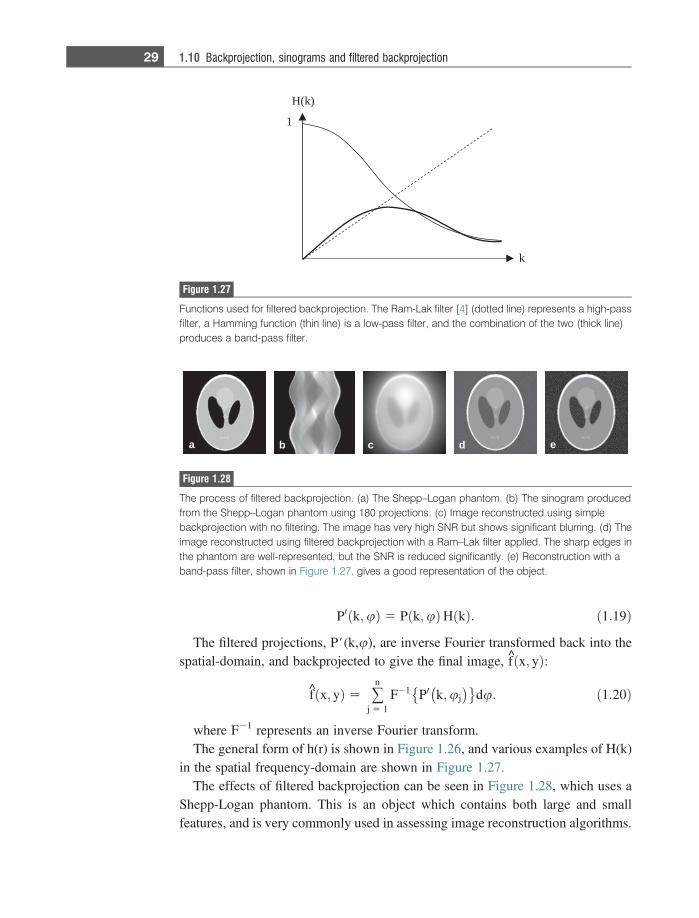
where F21 represents an inverse Fourier transform.The general form of h(r) is shown in Figure 1.26, and various examples of H(k)
in the spatial frequency-domain are shown in Figure 1.27.The effects of filtered backprojection can be seen in Figure 1.28, which uses a
Shepp-Logan phantom. This is an object which contains both large and smallfeatures, and is very commonly used in assessing image reconstruction algorithms.
H(k)
k
1
Figure 1.27
Functions used for filtered backprojection. The Ram-Lak filter [4] (dotted line) represents a high-passfilter, a Hamming function (thin line) is a low-pass filter, and the combination of the two (thick line)produces a band-pass filter.
a b c d e
Figure 1.28
The process of filtered backprojection. (a) The Shepp–Logan phantom. (b) The sinogram producedfrom the Shepp–Logan phantom using 180 projections. (c) Image reconstructed using simplebackprojection with no filtering. The image has very high SNR but shows significant blurring. (d) Theimage reconstructed using filtered backprojection with a Ram–Lak filter applied. The sharp edges inthe phantom are well-represented, but the SNR is reduced significantly. (e) Reconstruction with aband-pass filter, shown in Figure 1.27, gives a good representation of the object.
29 1.10 Backprojection, sinograms and filtered backprojection

The various shapes represent different features within the brain, including theskull, ventricles and several small features either overlapping other structures orplaced close together.
Exercises
Specificity, sensitivity and the ROC1.1 In a patient study for a new test for multiple sclerosis (MS), 32 of the 100
patients studied actually have MS. For the data given below, complete the two-by-two matrices and construct an ROC. The number of lesions (50, 40, 30, 20or 10) corresponds to the threshold value for designating MS as the diagnosis.
2 0
50 lesions 40 lesions
8 1
30 lesions
16 3
20 lesions
22 6
10 lesions
28 12
1.2 Choose a medical condition and suggest a clinical test which would have:(a) High sensitivity but low specificity;(b) Low sensitivity but high specificity.
1.3. What does an ROC curve that lies below the random line suggest? Could thisbe diagnostically useful?
Spatial resolution1.4 For the one-dimensional objects O(x) and PSFs h(x) shown in Figure 1.29,
draw the resulting projections I(x). Write down whether each object contains
O(x) I(x)h(x)
a
b
c
d
Figure 1.29
See Exercise 1.4.
30 General image characteristics

high, low or both spatial frequencies, and which is affected most by theaction of h(x).
1.5 Show mathematically that the FWHM of a Gaussian function is given by:
FWHM 5 2ffiffiffiffiffiffiffiffiffiffiffi2 ln 2p� �
r ffi 2:36r:
1.6 Plot the MTF on a single graph for each of the convolution filters shownbelow.
1
1 1
1 1
12
1 1 1
1
1 1
1 1
4
1 1 1
1
1 1
1 1
1
1 1 1
1.7 What type of filter is represented by the following kernel?
1
1 -1
0 -1
0
1 0 -1
1.8 Using the filter in Exercise 1.7 calculate the filtered image using the originalimage from Figure 1.11.
Data acquisition1.9 An ultrasound signal is digitized using a 16-bit ADC at a sampling rate of 3
MHz. If the image takes 20 ms to acquire, how much data (in Mbytes) is therein each ultrasound image. If images are acquired for 20 s continuously, whatis the total data output of the scan?
1.10 If a signal is digitized at a sampling rate of 20 kHz centred at 10 kHz, at whatfrequency would a signal at 22 kHz appear?
1.11 A signal is sampled every 1 ms for 20 ms, with the following actual values ofthe analogue voltage at successive sampling times. Plot the values of thevoltage recorded by a 5 volt, 4-bit ADC assuming that the noise level is muchlower than the signal and so can be neglected. On the same graph, plot thequantization error.
31 Exercises
SignalðvoltsÞ 5 �4:3; 1 1:2;�0:6;�0:9; 1 3:4;�2:7; 1 4:3; 1 0:1;�3:2;
�4:6; 1 1:8; 1 3:6; 1 2:4;�2:7; 1 0:5;�0:5;�3:7; 1 2:1;�4:1;�0:4
1.12 Using the same signal as in exercise 1.11, plot the values of the voltage andthe quantization error recorded by a 5 volt, 8-bit ADC.
Fourier transforms1.13 In Figure 1.20 plot the time and frequency domain signals for the case where
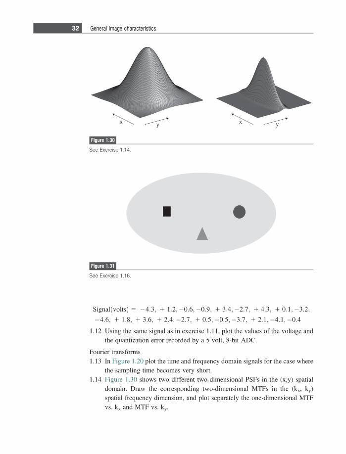
the sampling time becomes very short.1.14 Figure 1.30 shows two different two-dimensional PSFs in the (x,y) spatial
domain. Draw the corresponding two-dimensional MTFs in the (kx, ky)spatial frequency dimension, and plot separately the one-dimensional MTFvs. kx and MTF vs. ky.
x y x y
Figure 1.30
See Exercise 1.14.
Figure 1.31
See Exercise 1.16.
32 General image characteristics
Backprojection1.15 For Figure 1.25, suggest one possible shape that could have produced the
sinogram.1.16 For the object shown in Figure 1.31: (a) draw the projections at angles of 0,
45, 90, and 135�, and (b) draw the sinogram from the object. Assume that adark area corresponds to an area of high signal.
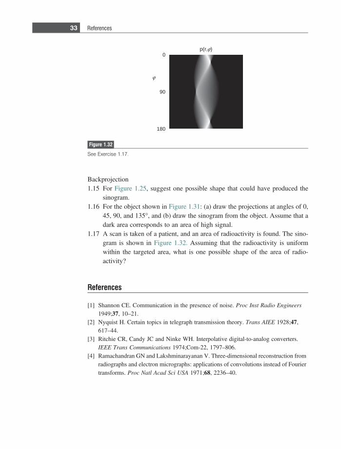
1.17 A scan is taken of a patient, and an area of radioactivity is found. The sino-gram is shown in Figure 1.32. Assuming that the radioactivity is uniformwithin the targeted area, what is one possible shape of the area of radio-activity?
References
[1] Shannon CE. Communication in the presence of noise. Proc Inst Radio Engineers
1949;37, 10–21.[2] Nyquist H. Certain topics in telegraph transmission theory. Trans AIEE 1928;47,
617–44.[3] Ritchie CR, Candy JC and Ninke WH. Interpolative digital-to-analog converters.
IEEE Trans Communications 1974;Com-22, 1797–806.[4] Ramachandran GN and Lakshminarayanan V. Three-dimensional reconstruction from
radiographs and electron micrographs: applications of convolutions instead of Fouriertransforms. Proc Natl Acad Sci USA 1971;68, 2236–40.
90
0
180
p(r, )
Figure 1.32
See Exercise 1.17.
33 References
2 X-ray planar radiography andcomputed tomography
2.1 Introduction
X-ray planar radiography is one of the mainstays of a radiology department,providing a first ‘screening’ for both acute injuries and suspected chronic diseases.Planar radiography is widely used to assess the degree of bone fracture in an acuteinjury, the presence of masses in lung cancer/emphysema and other airway path-ologies, the presence of kidney stones, and diseases of the gastrointestinal (GI)tract. Depending upon the results of an X-ray scan, the patient may be referred for afull three-dimensional X-ray computed tomography (CT) scan for more detaileddiagnosis.
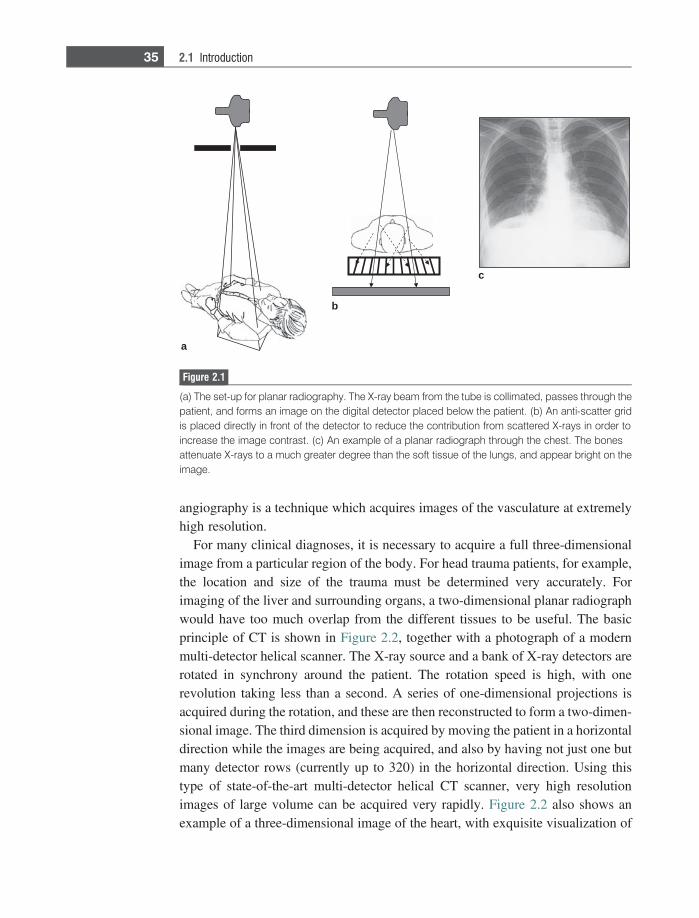
The basis of both planar radiography and CT is the differential absorption ofX-rays by various tissues. For example, bone and small calcifications absorb X-rays much more effectively than soft tissue. X-rays generated from a source aredirected towards the patient, as shown in Figure 2.1(a). X-rays which pass throughthe patient are detected using a solid-state flat panel detector which is placed justbelow the patient. The detected X-ray energy is first converted into light, then intoa voltage and finally is digitized. The digital image represents a two-dimensionalprojection of the tissues lying between the X-ray source and the detector. Inaddition to being absorbed, X-rays can also be scattered as they pass throughthe body, and this gives rise to a background signal which reduces the imagecontrast. Therefore, an ‘anti-scatter grid’, shown in Figure 2.1(b), is used to ensurethat only X-rays that pass directly through the body from source-to-detector arerecorded. An example of a two-dimensional planar X-ray is shown in Figure2.1(c). There is very high contrast, for example, between the bones (white) whichabsorb X-rays, and the lung tissue (dark) which absorbs very few X-rays.
There are a number of specialized applications of radiography which requirerelated but modified instrumentation. X-ray fluoroscopy is a technique in whichimages are continuously acquired to study, for example, the passage of anX-ray contrast agent through the GI tract. Digital mammography uses muchlower X-ray energies than standard X-ray scans, and is used to obtain images withmuch finer resolution than standard planar radiography. Digital subtraction
angiography is a technique which acquires images of the vasculature at extremelyhigh resolution.
For many clinical diagnoses, it is necessary to acquire a full three-dimensionalimage from a particular region of the body. For head trauma patients, for example,the location and size of the trauma must be determined very accurately. Forimaging of the liver and surrounding organs, a two-dimensional planar radiographwould have too much overlap from the different tissues to be useful. The basicprinciple of CT is shown in Figure 2.2, together with a photograph of a modernmulti-detector helical scanner. The X-ray source and a bank of X-ray detectors arerotated in synchrony around the patient. The rotation speed is high, with onerevolution taking less than a second. A series of one-dimensional projections isacquired during the rotation, and these are then reconstructed to form a two-dimen-sional image. The third dimension is acquired by moving the patient in a horizontaldirection while the images are being acquired, and also by having not just one butmany detector rows (currently up to 320) in the horizontal direction. Using thistype of state-of-the-art multi-detector helical CT scanner, very high resolutionimages of large volume can be acquired very rapidly. Figure 2.2 also shows anexample of a three-dimensional image of the heart, with exquisite visualization of
a
b
c
Figure 2.1
(a) The set-up for planar radiography. The X-ray beam from the tube is collimated, passes through thepatient, and forms an image on the digital detector placed below the patient. (b) An anti-scatter gridis placed directly in front of the detector to reduce the contribution from scattered X-rays in order toincrease the image contrast. (c) An example of a planar radiograph through the chest. The bonesattenuate X-rays to a much greater degree than the soft tissue of the lungs, and appear bright on theimage.
35 2.1 Introduction
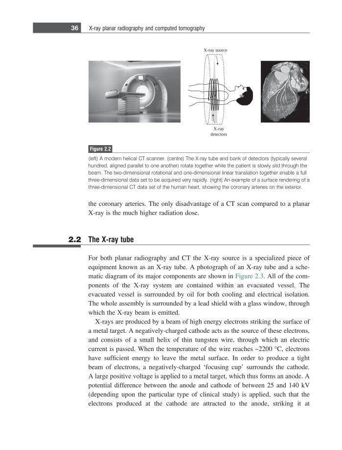
the coronary arteries. The only disadvantage of a CT scan compared to a planarX-ray is the much higher radiation dose.
2.2 The X-ray tube
For both planar radiography and CT the X-ray source is a specialized piece ofequipment known as an X-ray tube. A photograph of an X-ray tube and a sche-matic diagram of its major components are shown in Figure 2.3. All of the com-ponents of the X-ray system are contained within an evacuated vessel. Theevacuated vessel is surrounded by oil for both cooling and electrical isolation.The whole assembly is surrounded by a lead shield with a glass window, throughwhich the X-ray beam is emitted.
X-rays are produced by a beam of high energy electrons striking the surface ofa metal target. A negatively-charged cathode acts as the source of these electrons,and consists of a small helix of thin tungsten wire, through which an electriccurrent is passed. When the temperature of the wire reaches ~2200 �C, electronshave sufficient energy to leave the metal surface. In order to produce a tightbeam of electrons, a negatively-charged ‘focusing cup’ surrounds the cathode.A large positive voltage is applied to a metal target, which thus forms an anode. Apotential difference between the anode and cathode of between 25 and 140 kV(depending upon the particular type of clinical study) is applied, such that theelectrons produced at the cathode are attracted to the anode, striking it at
X-ray source
X-raydetectors
Figure 2.2
(left) A modern helical CT scanner. (centre) The X-ray tube and bank of detectors (typically severalhundred, aligned parallel to one another) rotate together while the patient is slowly slid through thebeam. The two-dimensional rotational and one-dimensional linear translation together enable a fullthree-dimensional data set to be acquired very rapidly. (right) An example of a surface rendering of athree-dimensional CT data set of the human heart, showing the coronary arteries on the exterior.
36 X-ray planar radiography and computed tomography
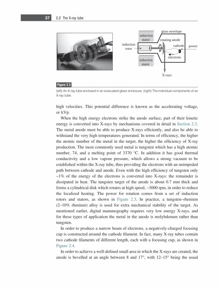
high velocities. This potential difference is known as the accelerating voltage,or kVp.
When the high energy electrons strike the anode surface, part of their kineticenergy is converted into X-rays by mechanisms covered in detail in Section 2.3.The metal anode must be able to produce X-rays efficiently, and also be able towithstand the very high temperatures generated. In terms of efficiency, the higherthe atomic number of the metal in the target, the higher the efficiency of X-rayproduction. The most commonly used metal is tungsten which has a high atomicnumber, 74, and a melting point of 3370 �C. In addition it has good thermalconductivity and a low vapour pressure, which allows a strong vacuum to beestablished within the X-ray tube, thus providing the electrons with an unimpededpath between cathode and anode. Even with the high efficiency of tungsten only~1% of the energy of the electrons is converted into X-rays: the remainder isdissipated in heat. The tungsten target of the anode is about 0.7 mm thick andforms a cylindrical disk which rotates at high speed, ~3000 rpm, in order to reducethe localized heating. The power for rotation comes from a set of inductionrotors and stators, as shown in Figure 2.3. In practice, a tungsten–rhenium(2–10% rhenium) alloy is used for extra mechanical stability of the target. Asmentioned earlier, digital mammography requires very low energy X-rays, andfor these types of application the metal in the anode is molybdenum rather thantungsten.
In order to produce a narrow beam of electrons, a negatively-charged focusingcup is constructed around the cathode filament. In fact, many X-ray tubes containtwo cathode filaments of different length, each with a focusing cup, as shown inFigure 2.4.
In order to achieve a well-defined small area in which the X-rays are created, theanode is bevelled at an angle between 8 and 17�, with 12–15� being the usual
inductionrotor
inductionstator
cathode
electrons
rotating anode
glass envelope
X-rays
inductionstator
power
Figure 2.3
(left) An X-ray tube enclosed in an evacuated glass enclosure. (right) The individual components of anX-ray tube.
37 2.2 The X-ray tube
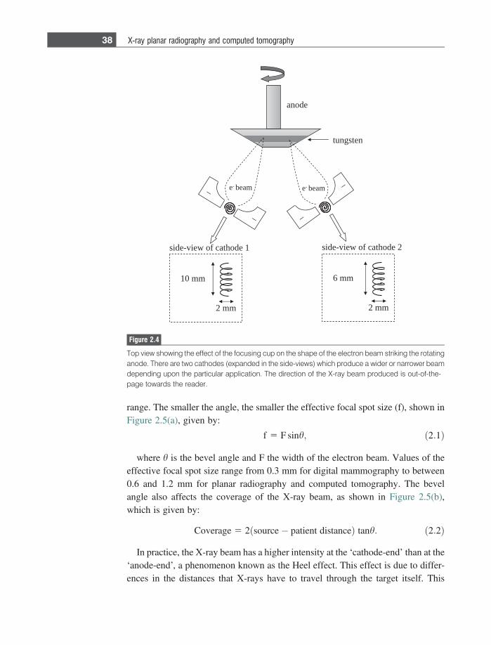
range. The smaller the angle, the smaller the effective focal spot size (f), shown inFigure 2.5(a), given by:
f 5 F sinh; ð2:1Þ
where h is the bevel angle and F the width of the electron beam. Values of theeffective focal spot size range from 0.3 mm for digital mammography to between0.6 and 1.2 mm for planar radiography and computed tomography. The bevelangle also affects the coverage of the X-ray beam, as shown in Figure 2.5(b),which is given by:
Coverage 5 2 source� patient distanceð Þ tanh: ð2:2Þ
In practice, the X-ray beam has a higher intensity at the ‘cathode-end’ than at the‘anode-end’, a phenomenon known as the Heel effect. This effect is due to differ-ences in the distances that X-rays have to travel through the target itself. This
edona
_
_ _
_
netsgnut
mm 01
mm 2
1 edohtac fo weiv-edis
mm 6
mm 2
2 edohtac fo weiv-edis
e- maeb e- maeb
Figure 2.4
Top view showing the effect of the focusing cup on the shape of the electron beam striking the rotatinganode. There are two cathodes (expanded in the side-views) which produce a wider or narrower beamdepending upon the particular application. The direction of the X-ray beam produced is out-of-the-page towards the reader.
38 X-ray planar radiography and computed tomography
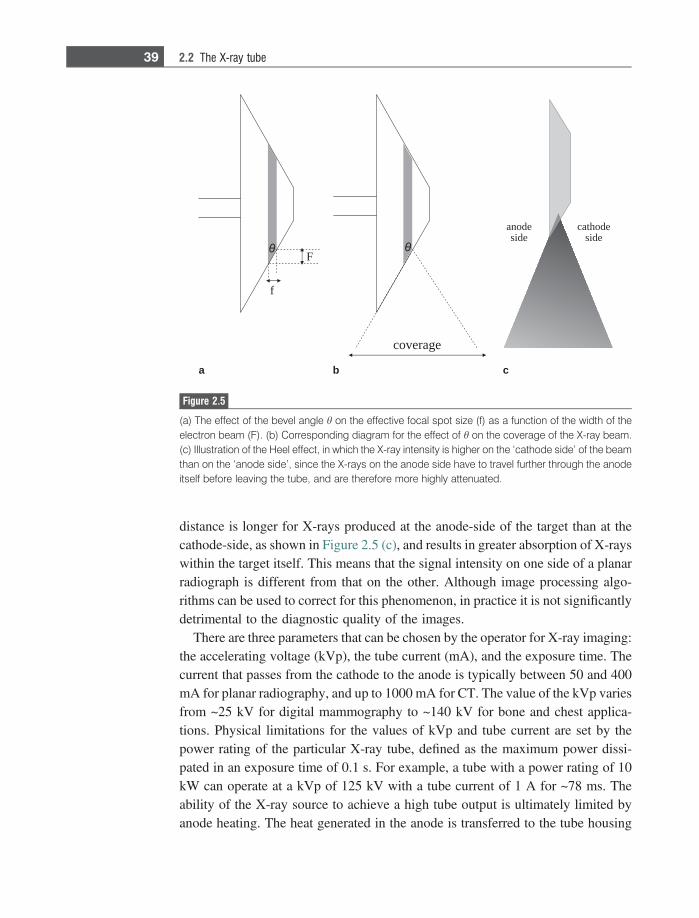
distance is longer for X-rays produced at the anode-side of the target than at thecathode-side, as shown in Figure 2.5 (c), and results in greater absorption of X-rayswithin the target itself. This means that the signal intensity on one side of a planarradiograph is different from that on the other. Although image processing algo-rithms can be used to correct for this phenomenon, in practice it is not significantlydetrimental to the diagnostic quality of the images.
There are three parameters that can be chosen by the operator for X-ray imaging:the accelerating voltage (kVp), the tube current (mA), and the exposure time. Thecurrent that passes from the cathode to the anode is typically between 50 and 400mA for planar radiography, and up to 1000 mA for CT. The value of the kVp variesfrom ~25 kV for digital mammography to ~140 kV for bone and chest applica-tions. Physical limitations for the values of kVp and tube current are set by thepower rating of the particular X-ray tube, defined as the maximum power dissi-pated in an exposure time of 0.1 s. For example, a tube with a power rating of 10kW can operate at a kVp of 125 kV with a tube current of 1 A for ~78 ms. Theability of the X-ray source to achieve a high tube output is ultimately limited byanode heating. The heat generated in the anode is transferred to the tube housing
coverage
F
f
anodeside
cathodeside
a b c
Figure 2.5
(a) The effect of the bevel angle h on the effective focal spot size (f) as a function of the width of theelectron beam (F). (b) Corresponding diagram for the effect of h on the coverage of the X-ray beam.(c) Illustration of the Heel effect, in which the X-ray intensity is higher on the ‘cathode side’ of the beamthan on the ‘anode side’, since the X-rays on the anode side have to travel further through the anodeitself before leaving the tube, and are therefore more highly attenuated.
39 2.2 The X-ray tube
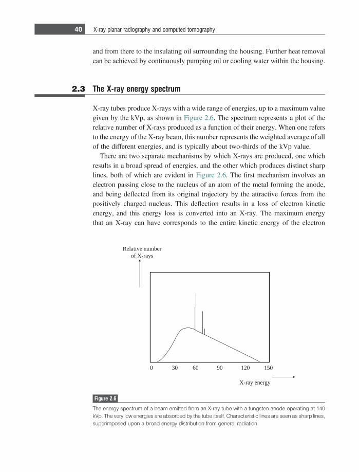
and from there to the insulating oil surrounding the housing. Further heat removalcan be achieved by continuously pumping oil or cooling water within the housing.
2.3 The X-ray energy spectrum
X-ray tubes produce X-rays with a wide range of energies, up to a maximum valuegiven by the kVp, as shown in Figure 2.6. The spectrum represents a plot of therelative number of X-rays produced as a function of their energy. When one refersto the energy of the X-ray beam, this number represents the weighted average of allof the different energies, and is typically about two-thirds of the kVp value.
There are two separate mechanisms by which X-rays are produced, one whichresults in a broad spread of energies, and the other which produces distinct sharplines, both of which are evident in Figure 2.6. The first mechanism involves anelectron passing close to the nucleus of an atom of the metal forming the anode,and being deflected from its original trajectory by the attractive forces from thepositively charged nucleus. This deflection results in a loss of electron kineticenergy, and this energy loss is converted into an X-ray. The maximum energythat an X-ray can have corresponds to the entire kinetic energy of the electron
0510210906030
rebmun evitaleRsyar-X fo
ygrene yar-X
Figure 2.6
The energy spectrum of a beam emitted from an X-ray tube with a tungsten anode operating at 140kVp. The very low energies are absorbed by the tube itself. Characteristic lines are seen as sharp lines,superimposed upon a broad energy distribution from general radiation.
40 X-ray planar radiography and computed tomography
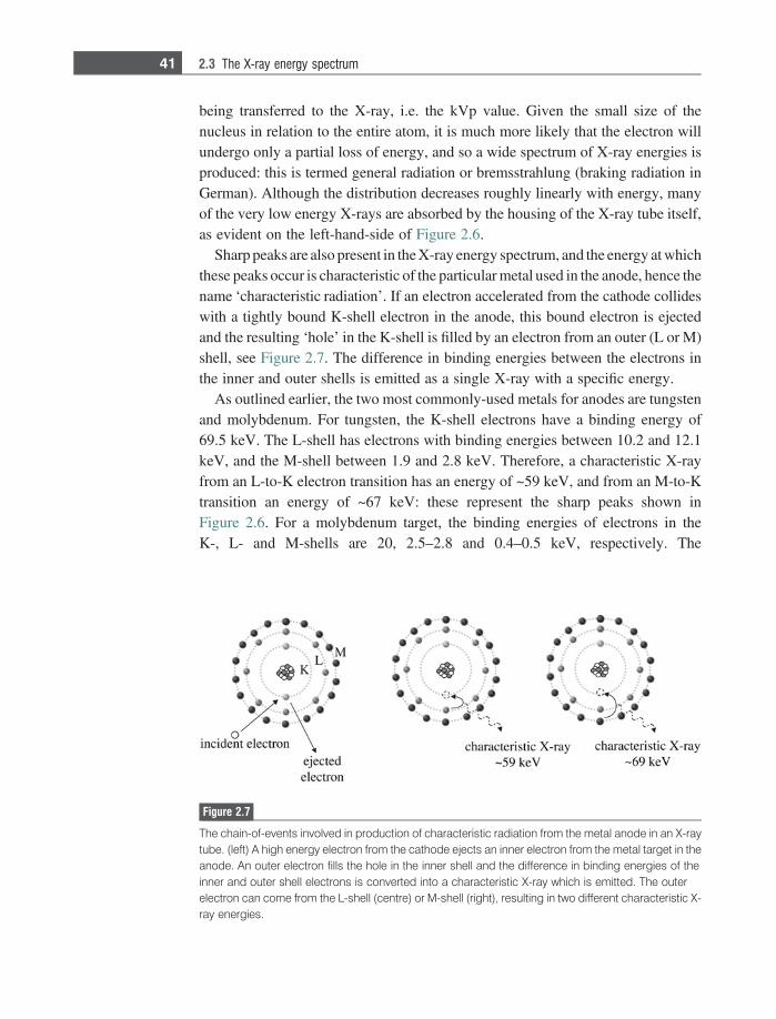
being transferred to the X-ray, i.e. the kVp value. Given the small size of thenucleus in relation to the entire atom, it is much more likely that the electron willundergo only a partial loss of energy, and so a wide spectrum of X-ray energies isproduced: this is termed general radiation or bremsstrahlung (braking radiation inGerman). Although the distribution decreases roughly linearly with energy, manyof the very low energy X-rays are absorbed by the housing of the X-ray tube itself,as evident on the left-hand-side of Figure 2.6.
Sharp peaks are also present in the X-ray energy spectrum, and the energy at whichthese peaks occur is characteristic of the particular metal used in the anode, hence thename ‘characteristic radiation’. If an electron accelerated from the cathode collideswith a tightly bound K-shell electron in the anode, this bound electron is ejectedand the resulting ‘hole’ in the K-shell is filled by an electron from an outer (L or M)shell, see Figure 2.7. The difference in binding energies between the electrons inthe inner and outer shells is emitted as a single X-ray with a specific energy.
As outlined earlier, the two most commonly-used metals for anodes are tungstenand molybdenum. For tungsten, the K-shell electrons have a binding energy of69.5 keV. The L-shell has electrons with binding energies between 10.2 and 12.1keV, and the M-shell between 1.9 and 2.8 keV. Therefore, a characteristic X-rayfrom an L-to-K electron transition has an energy of ~59 keV, and from an M-to-Ktransition an energy of ~67 keV: these represent the sharp peaks shown inFigure 2.6. For a molybdenum target, the binding energies of electrons in theK-, L- and M-shells are 20, 2.5–2.8 and 0.4–0.5 keV, respectively. The
Figure 2.7
The chain-of-events involved in production of characteristic radiation from the metal anode in an X-raytube. (left) A high energy electron from the cathode ejects an inner electron from the metal target in theanode. An outer electron fills the hole in the inner shell and the difference in binding energies of theinner and outer shell electrons is converted into a characteristic X-ray which is emitted. The outerelectron can come from the L-shell (centre) or M-shell (right), resulting in two different characteristic X-ray energies.
41 2.3 The X-ray energy spectrum
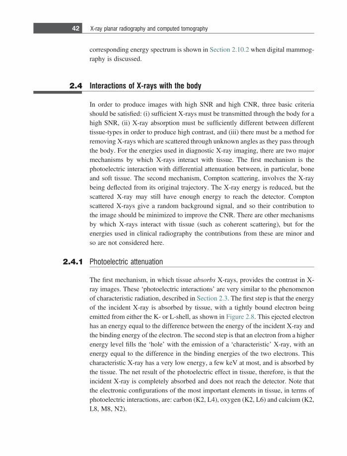
corresponding energy spectrum is shown in Section 2.10.2 when digital mammog-raphy is discussed.
2.4 Interactions of X-rays with the body
In order to produce images with high SNR and high CNR, three basic criteriashould be satisfied: (i) sufficient X-rays must be transmitted through the body for ahigh SNR, (ii) X-ray absorption must be sufficiently different between differenttissue-types in order to produce high contrast, and (iii) there must be a method forremoving X-rays which are scattered through unknown angles as they pass throughthe body. For the energies used in diagnostic X-ray imaging, there are two majormechanisms by which X-rays interact with tissue. The first mechanism is thephotoelectric interaction with differential attenuation between, in particular, boneand soft tissue. The second mechanism, Compton scattering, involves the X-raybeing deflected from its original trajectory. The X-ray energy is reduced, but thescattered X-ray may still have enough energy to reach the detector. Comptonscattered X-rays give a random background signal, and so their contribution tothe image should be minimized to improve the CNR. There are other mechanismsby which X-rays interact with tissue (such as coherent scattering), but for theenergies used in clinical radiography the contributions from these are minor andso are not considered here.
2.4.1 Photoelectric attenuation
The first mechanism, in which tissue absorbs X-rays, provides the contrast in X-ray images. These ‘photoelectric interactions’ are very similar to the phenomenonof characteristic radiation, described in Section 2.3. The first step is that the energyof the incident X-ray is absorbed by tissue, with a tightly bound electron beingemitted from either the K- or L-shell, as shown in Figure 2.8. This ejected electronhas an energy equal to the difference between the energy of the incident X-ray andthe binding energy of the electron. The second step is that an electron from a higherenergy level fills the ‘hole’ with the emission of a ‘characteristic’ X-ray, with anenergy equal to the difference in the binding energies of the two electrons. Thischaracteristic X-ray has a very low energy, a few keV at most, and is absorbed bythe tissue. The net result of the photoelectric effect in tissue, therefore, is that theincident X-ray is completely absorbed and does not reach the detector. Note thatthe electronic configurations of the most important elements in tissue, in terms ofphotoelectric interactions, are: carbon (K2, L4), oxygen (K2, L6) and calcium (K2,L8, M8, N2).
42 X-ray planar radiography and computed tomography

The probability of a photoelectric interaction (Ppe) occurring depends on theenergy (E) of the incident X-ray, the effective atomic number (Zeff) of the tissue,and the tissue density (q):
Ppe } qZ3
eff
E3 : ð2:3Þ
The effective atomic number of tissue is ~7.4, of lipid ~6.9, and of bone ~13.8(the high value is due primarily to the presence of calcium). The relative densitiesare 1: 0.9: 1.85. Equation (2.3) indicates that, at low X-ray energies, the photo-electric effect produces high constrast between bone (high attenuation) and softtissue (low attenuation), but that the contrast decreases with increasing X-rayenergy. This is further expanded upon in Section 2.5.
2.4.2 Compton scattering
Compton scattering refers to the interaction between an incident X-ray and aloosely bound electron in an outer shell of an atom in tissue. In Compton scatteringa small fraction of the incident X-ray energy is transferred to this loosely-boundelectron. With the additional energy, the electron is ejected, and the X-ray isdeflected from its original path by an angle h, as shown in Figure 2.9.
The energy of the scattered X-ray can be calculated by applying the lawsof conservation of momentum and energy. The standard Compton equation com-putes the change in wavelength between the incident and scattered X-ray, which isgiven by:
Figure 2.8
A photoelectric interaction between an incident X-ray and tissue involves an inner electron beingemitted (left), an electron from an outer shell filling the hole in the inner shell (middle), and thedifference in the binding energies being transferred to a characteristic X-ray. This X-ray has very lowenergy and is absorbed after travelling ~1 mm in tissue.
43 2.4 Interactions of X-rays with the body

Dk 5h
m0c1� coshð Þ; ð2:4Þ
where m0 is the rest mass of the ejected electron, and c is the speed of light. Thischange in wavelength can easily be converted into the relevant loss in energy (DE):
DE 5 EX;inc � EX;scat 5hckinc� hc
kscat: ð2:5Þ
The energy of the scattered X-ray is then given by:
EX;scat 5EX;inc
1 1EX;inc
mc2
� �1� coshð Þ
: ð2:6Þ
Figure 2.10 shows a graph of scattered X-ray energy vs. scatter angle for anincident energy of 70 keV. As can be seen from the graph, the energy of the X-rayis reduced only by a very small amount even for quite large deflection angles, andso it is very likely that it will pass through the body and be detected as if it wereprimary radiation, i.e. radiation which has not been scattered at all. Of course, if thescatter angle is very large the trajectory of the scattered X-ray will miss thedetector, and the X-ray will effectively have been attenuated.
The probability of an X-ray undergoing Compton scattering is, to first order,independent of atomic number, is proportional to the tissue electron density, and isonly weakly dependent on the energy of the incident X-ray.
At low X-ray energies, the photoelectric effect dominates over Comptonscattering. Since the Zeff of bone is approximately twice that of tissue, there isfar greater attenuation in bone than in tissue, and excellent tissue contrast. How-ever, at higher X-ray energies the contribution from Compton scattering becomes
incident X-ray
scattered X-ray
ejectedelectron
X-ray
scatteredX-ray
electron
EX,inc
EX,scatpX,scat
Figure 2.9
Compton scattering of an incident X-ray involves an outer electron being ejected from a tissuemolecule (left), with the X-ray being scattered at an angle h with respect to its initial trajectory (right).
44 X-ray planar radiography and computed tomography
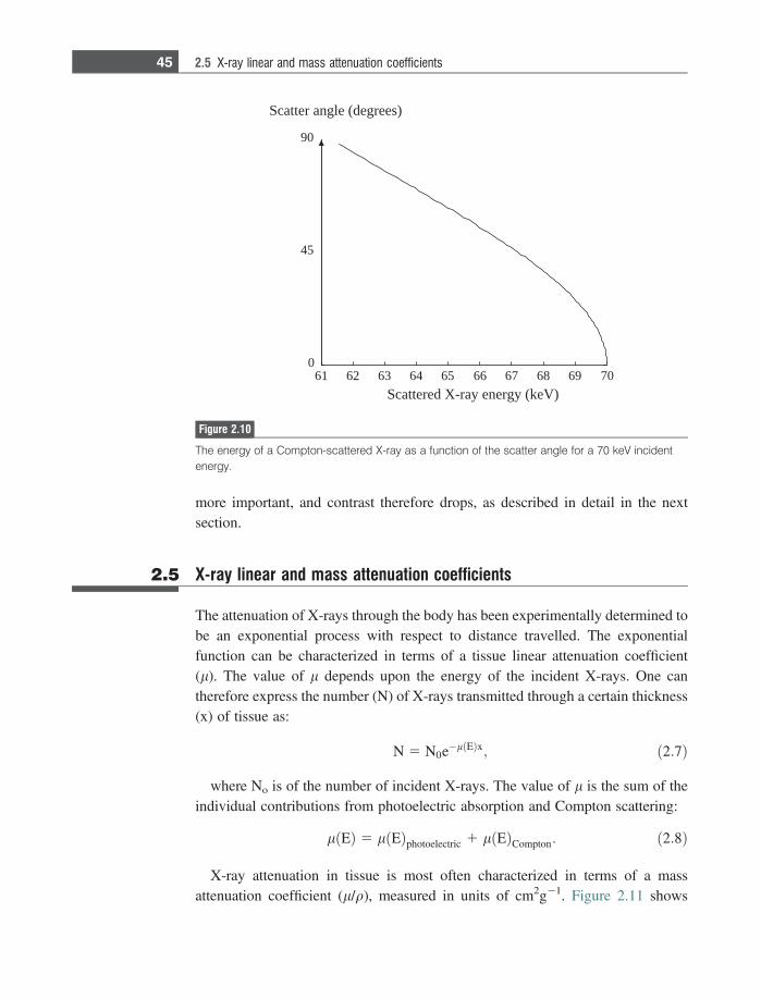
more important, and contrast therefore drops, as described in detail in the nextsection.
2.5 X-ray linear and mass attenuation coefficients
The attenuation of X-rays through the body has been experimentally determined tobe an exponential process with respect to distance travelled. The exponentialfunction can be characterized in terms of a tissue linear attenuation coefficient(l). The value of l depends upon the energy of the incident X-rays. One cantherefore express the number (N) of X-rays transmitted through a certain thickness(x) of tissue as:
N 5 N0e�l Eð Þx; ð2:7Þ
where No is of the number of incident X-rays. The value of l is the sum of theindividual contributions from photoelectric absorption and Compton scattering:
l Eð Þ 5 l Eð Þphotoelectric 1 l Eð ÞCompton: ð2:8Þ
X-ray attenuation in tissue is most often characterized in terms of a massattenuation coefficient (l/q), measured in units of cm2g21. Figure 2.11 shows
61 62 63 64 65 66 67 68 69 700
45
90
Scattered X-ray energy (keV)
Scatter angle (degrees)
Figure 2.10
The energy of a Compton-scattered X-ray as a function of the scatter angle for a 70 keV incidentenergy.
45 2.5 X-ray linear and mass attenuation coefficients
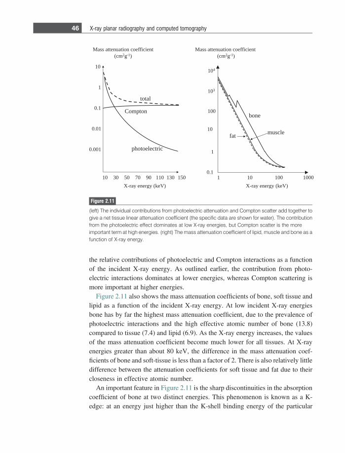
the relative contributions of photoelectric and Compton interactions as a functionof the incident X-ray energy. As outlined earlier, the contribution from photo-electric interactions dominates at lower energies, whereas Compton scattering ismore important at higher energies.
Figure 2.11 also shows the mass attenuation coefficients of bone, soft tissue andlipid as a function of the incident X-ray energy. At low incident X-ray energiesbone has by far the highest mass attenuation coefficient, due to the prevalence ofphotoelectric interactions and the high effective atomic number of bone (13.8)compared to tissue (7.4) and lipid (6.9). As the X-ray energy increases, the valuesof the mass attenuation coefficient become much lower for all tissues. At X-rayenergies greater than about 80 keV, the difference in the mass attenuation coef-ficients of bone and soft-tissue is less than a factor of 2. There is also relatively littledifference between the attenuation coefficients for soft tissue and fat due to theircloseness in effective atomic number.
An important feature in Figure 2.11 is the sharp discontinuities in the absorptioncoefficient of bone at two distinct energies. This phenomenon is known as a K-edge: at an energy just higher than the K-shell binding energy of the particular
0510310110907050301
01
1
1.0
10.0
100.0 cirtceleotohp
tneiciffeoc noitaunetta ssaMmc( 2g 1- )
notpmoC
latot
)Vek( ygrene yar-X
tneiciffeoc noitaunetta ssaMmc( 2g 1- )
)Vek( ygrene yar-X
tafelcsum
enob
1.0
1
01
1
001
01 3
01 4
000100101
Figure 2.11
(left) The individual contributions from photoelectric attenuation and Compton scatter add together togive a net tissue linear attenuation coefficient (the specific data are shown for water). The contributionfrom the photoelectric effect dominates at low X-ray energies, but Compton scatter is the moreimportant term at high energies. (right) The mass attenuation coefficient of lipid, muscle and bone as afunction of X-ray energy.
46 X-ray planar radiography and computed tomography
atom (calcium for bone), the probability of photoelectric interactions increasesdramatically, typically by a factor of 5 to 8. One can see that, without these jumps,the attenuation of bone would be very similar to that of muscle and lipid. Thephenomenon of a K-edge is also critical in the design of both X-ray contrast agentsand X-ray detectors, which are covered later in this chapter.
The attenuation properties of tissue can also be described in terms of the half-value layer (HVL), which as the name suggests is the thickness of tissue whichreduces the intensity of the X-ray beam by a factor of one-half. From Equation(2.7), the value of the HVL is given by (ln 2)/l. At an X-ray energy of 100 keV,for example, the HVL for muscle is 3.9 cm and for bone is 2.3 cm: the corres-ponding numbers at 30 keV (relevant for mammography) are 1.8 cm and 0.4 cm,respectively.
Example 2.1 If the thickness of the chest is 20 cm, what percentage of X-rays are transmittedthrough the chest at an incident X-ray energy of 70 keV assuming HVL valuesof 3.5 and 1.8 cm21 for muscle and bone, respectively, and the bone thickness to be4 cm and the tissue thickness 16 cm?
Solution For the muscle, the value of l is given by (ln 2)/3.5~0.2 cm21. For 16 cm of tissue:
NN0
5 e� 0:2ð Þ16 5 0:04:
For bone the value of l is (ln 2)/1.8~0.4 cm21. For 4 cm of bone:
NN0
5 e� 0:4ð Þ4 5 0:2:
Therefore, overall the percentage is given by 100 3 (0.2 3 0.04) = 0.8%.
2.6 Instrumentation for planar radiography
In addition to the X-ray tube, the other basic components of a planar X-rayradiography system are: (i) a collimator to reduce the patient dose and amountof Compton scattered X-rays, (ii) an anti-scatter grid to reduce further the contri-bution of scattered X-rays to the image, and (iii) a digital detector which convertsthe energy of the transmitted X-rays into light: the light is then converted into avoltage using photodiodes, and this voltage is digitized using an analogue-to-digital converter, as covered in Chapter 1.
47 2.6 Instrumentation for planar radiography
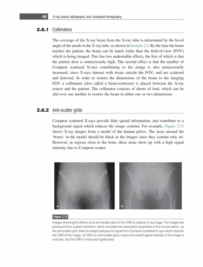
2.6.1 Collimators
The coverage of the X-ray beam from the X-ray tube is determined by the bevelangle of the anode in the X-ray tube, as shown in Section 2.2. By the time the beamreaches the patient, the beam can be much wider than the field-of-view (FOV)which is being imaged. This has two undesirable effects, the first of which is thatthe patient dose is unnecessarily high. The second effect is that the number ofCompton scattered X-rays contributing to the image is also unnecessarilyincreased, since X-rays interact with tissue outside the FOV, and are scatteredand detected. In order to restrict the dimensions of the beam to the imagingFOV a collimator (also called a beam-restrictor) is placed between the X-raysource and the patient. The collimator consists of sheets of lead, which can beslid over one another to restrict the beam in either one or two dimensions.
2.6.2 Anti-scatter grids
Compton scattered X-rays provide little spatial information, and contribute to abackground signal which reduces the image contrast. For example, Figure 2.12shows X-ray images from a model of the human pelvis. The areas around the‘bones’ in the model should be black in the images since they contain only air.However, in regions close to the bone, these areas show up with a high signalintensity due to Compton scatter.
a b
Figure 2.12
Images showing the effects of an anti-scatter grid on the CNR of a planar X-ray image. The images areproduced from a pelvic phantom, which simulates the absorption properties of the human pelvis. (a)No anti-scatter grid: there is a large background signal from Compton-scattered X-rays which reducesthe CNR of the image. (b) With an anti-scatter grid in place the overall signal intensity of the image isreduced, but the CNR is improved significantly.
48 X-ray planar radiography and computed tomography
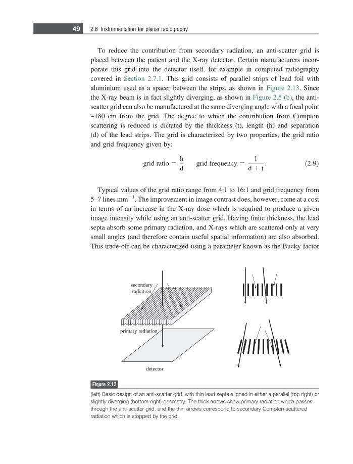
To reduce the contribution from secondary radiation, an anti-scatter grid isplaced between the patient and the X-ray detector. Certain manufacturers incor-porate this grid into the detector itself, for example in computed radiographycovered in Section 2.7.1. This grid consists of parallel strips of lead foil withaluminium used as a spacer between the strips, as shown in Figure 2.13. Sincethe X-ray beam is in fact slightly diverging, as shown in Figure 2.5 (b), the anti-scatter grid can also be manufactured at the same diverging angle with a focal point~180 cm from the grid. The degree to which the contribution from Comptonscattering is reduced is dictated by the thickness (t), length (h) and separation(d) of the lead strips. The grid is characterized by two properties, the grid ratioand grid frequency given by:
grid ratio 5hd
grid frequency 51
d 1 t: ð2:9Þ
Typical values of the grid ratio range from 4:1 to 16:1 and grid frequency from5–7 lines mm21. The improvement in image contrast does, however, come at a costin terms of an increase in the X-ray dose which is required to produce a givenimage intensity while using an anti-scatter grid. Having finite thickness, the leadsepta absorb some primary radiation, and X-rays which are scattered only at verysmall angles (and therefore contain useful spatial information) are also absorbed.This trade-off can be characterized using a parameter known as the Bucky factor
noitaidar yramirp
rotceted
yradnocesnoitaidar
Figure 2.13
(left) Basic design of an anti-scatter grid, with thin lead septa aligned in either a parallel (top right) orslightly diverging (bottom right) geometry. The thick arrows show primary radiation which passesthrough the anti-scatter grid, and the thin arrows correspond to secondary Compton-scatteredradiation which is stopped by the grid.
49 2.6 Instrumentation for planar radiography
(BF). If an equal X-ray dose is incident upon the detector in the presence andabsence of an anti-scatter grid, then the dose that is delivered to the patientincreases by a factor BF. Typical values of BF are between 4 and 10. In Figure2.12(b), for example, the image contrast is improved significantly by use of an anti-scatter grid: however, the X-ray dose to the patient is almost ten times higher thanfor the image in Figure 2.12(a) acquired without an anti-scatter grid.
2.7 X-ray detectors
Traditional X-ray film is essentially a thing of the past, with current diagnosesbeing performed almost exclusively from digital images displayed on high reso-lution computer screens. In addition to the higher quality images made possibleusing digital detectors, the ability to store and transfer images easily through largemedical data centres via so-called picture archiving and communication systems(PACS) has become extremely important. There are two basic digital detectortechnologies which are currently used, computed radiography and digital radiog-raphy. The former is currently cheaper and more widespread, but is anticipated tobe superseded by the latter technology within the next decade, especially as thecosts of digital radiography fall.
2.7.1 Computed radiography
Computed radiography (CR) instrumentation consists of a detector plate and aCR reader which digitizes the plate after the X-ray image has been acquired.The CR plate consists of a thin layer of phosphor crystals, most commonlybarium fluorohalide activated with europium ions (BaFX:Eu2+), where the halideX is a mixture of bromine and iodine. The plate size ranges from 18 3 24 cm formammography to 35 3 43 cm for chest radiography. The plates can be categorizedas either high resolution (HR), usually used for mammography, or standard forgeneral applications. Note that HR plates have a thinner phosphor layer (~140 lm)compared to standard plates (230 lm), and the phosphor crystals are physicallysmaller [1].
The CR plates convert the X-rays which pass through the patient and the anti-scatter grid into light. When X-rays strike the plate they release electrons in thephosphor layer: these electrons are trapped for a timescale of hours in sites formedby dislocations in the phosphor crystal lattice. This effectively forms a ‘latent’image, i.e. one which is present but is not immediately visible. The CR plate isprotected by a light-tight cassette which is transparent to X-rays. After the image
50 X-ray planar radiography and computed tomography
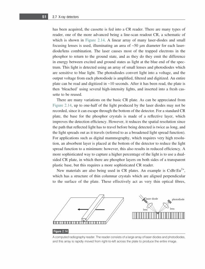
has been acquired, the cassette is fed into a CR reader. There are many types ofreader, one of the more advanced being a line-scan readout CR, a schematic ofwhich is shown in Figure 2.14. A linear array of many laser-diodes and smallfocusing lenses is used, illuminating an area of ~50 lm diameter for each laser-diode/lens combination. The laser causes most of the trapped electrons in thephosphor to return to the ground state, and as they do they emit the differencein energy between excited and ground states as light at the blue end of the spec-trum. This light is detected using an array of small lenses and photodiodes whichare sensitive to blue light. The photodiodes convert light into a voltage, and theoutput voltage from each photodiode is amplified, filtered and digitized. An entireplate can be read and digitized in ~10 seconds. After it has been read, the plate isthen ‘bleached’ using several high-intensity lights, and inserted into a fresh cas-sette to be reused.
There are many variations on the basic CR plate. As can be appreciated fromFigure 2.14, up to one-half of the light produced by the laser diodes may not berecorded, since it can escape through the bottom of the detector. For a standard CRplate, the base for the phosphor crystals is made of a reflective layer, whichimproves the detection efficiency. However, it reduces the spatial resolution sincethe path that reflected light has to travel before being detected is twice as long, andthe light spreads out as it travels (referred to as a broadened light spread function).For applications such as digital mammography, which requires very high resolu-tion, an absorbent layer is placed at the bottom of the detector to reduce the lightspread function to a minimum: however, this also results in reduced efficiency. Amore sophisticated way to capture a higher percentage of the light is to use a dual-sided CR plate, in which there are phosphor layers on both sides of a transparentplastic base, but this requires a more sophisticated CR reader.
New materials are also being used in CR plates. An example is CsBr:Eu2+,which has a structure of thin columnar crystals which are aligned perpendicularto the surface of the plate. These effectively act as very thin optical fibres,
edoid resal
snel snel
edoidotohp
Figure 2.14
A computed radiography reader. The reader consists of a large array of laser diodes and photodiodes,and this array is rapidly moved from right-to-left across the plate to produce the entire image.
51 2.7 X-ray detectors
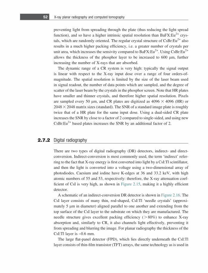
preventing light from spreading through the plate (thus reducing the light spreadfunction), and so have a higher intrinsic spatial resolution than BaFX:Eu2+ crys-tals, which are randomly oriented. The regular crystal structure of CsBr:Eu2+ alsoresults in a much higher packing efficiency, i.e. a greater number of crystals perunit area, which increases the sensivity compared to BaFX:Eu2+. Using CsBr:Eu2+
allows the thickness of the phosphor layer to be increased to 600 lm, furtherincreasing the number of X-rays that are absorbed.
The dynamic range of a CR system is very high: typically the signal outputis linear with respect to the X-ray input dose over a range of four orders-of-magnitude. The spatial resolution is limited by the size of the laser beam usedin signal readout, the number of data points which are sampled, and the degree ofscatter of the laser beam by the crystals in the phosphor screen. Note that HR plateshave smaller and thinner crystals, and therefore higher spatial resolution. Pixelsare sampled every 50 lm, and CR plates are digitized as 4096 3 4096 (HR) or2048 3 2048 matrix sizes (standard). The SNR of a standard image plate is roughlytwice that of a HR plate for the same input dose. Using a dual-sided CR plateincreases the SNR by close to a factor of 2 compared to single-sided, and using newCsBr:Eu2+ based plates increases the SNR by an additional factor of 2.
2.7.2 Digital radiography
There are two types of digital radiography (DR) detectors, indirect- and direct-conversion. Indirect-conversion is most commonly used, the term ‘indirect’ refer-ring to the fact that X-ray energy is first converted into light by a CsI:Tl scintillator,and then the light is converted into a voltage using a two-dimensional array ofphotodiodes. Caesium and iodine have K-edges at 36 and 33.2 keV, with highatomic numbers of 55 and 53, respectively: therefore, the X-ray attenuation coef-ficient of CsI is very high, as shown in Figure 2.15, making it a highly efficientdetector.
A schematic of an indirect-conversion DR detector is shown in Figure 2.16. TheCsI layer consists of many thin, rod-shaped, CsI:Tl ‘needle crystals’ (approxi-mately 5 lm in diameter) aligned parallel to one another and extending from thetop surface of the CsI layer to the substrate on which they are manufactured. Theneedle structure gives excellent packing efficiency (.80%) to enhance X-rayabsorption and, similarly to CR, it also channels light effectively, preventing itfrom spreading and blurring the image. For planar radiography the thickness of theCsI:Tl layer is ~0.6 mm.
The large flat-panel detector (FPD), which lies directly underneath the CsI:Tllayer consists of thin-film transistor (TFT) arrays, the same technology as is used in
52 X-ray planar radiography and computed tomography
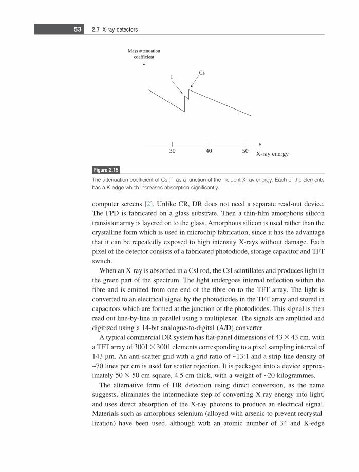
computer screens [2]. Unlike CR, DR does not need a separate read-out device.The FPD is fabricated on a glass substrate. Then a thin-film amorphous silicontransistor array is layered on to the glass. Amorphous silicon is used rather than thecrystalline form which is used in microchip fabrication, since it has the advantagethat it can be repeatedly exposed to high intensity X-rays without damage. Eachpixel of the detector consists of a fabricated photodiode, storage capacitor and TFTswitch.
When an X-ray is absorbed in a CsI rod, the CsI scintillates and produces light inthe green part of the spectrum. The light undergoes internal reflection within thefibre and is emitted from one end of the fibre on to the TFT array. The light isconverted to an electrical signal by the photodiodes in the TFT array and stored incapacitors which are formed at the junction of the photodiodes. This signal is thenread out line-by-line in parallel using a multiplexer. The signals are amplified anddigitized using a 14-bit analogue-to-digital (A/D) converter.
A typical commercial DR system has flat-panel dimensions of 43 3 43 cm, witha TFT array of 3001 3 3001 elements corresponding to a pixel sampling interval of143 lm. An anti-scatter grid with a grid ratio of ~13:1 and a strip line density of~70 lines per cm is used for scatter rejection. It is packaged into a device approx-imately 50 3 50 cm square, 4.5 cm thick, with a weight of ~20 kilogrammes.
The alternative form of DR detection using direct conversion, as the namesuggests, eliminates the intermediate step of converting X-ray energy into light,and uses direct absorption of the X-ray photons to produce an electrical signal.Materials such as amorphous selenium (alloyed with arsenic to prevent recrystal-lization) have been used, although with an atomic number of 34 and K-edge
Mass attenuationcoefficient
CsI
4030 50 X-ray energy
Figure 2.15
The attenuation coefficient of CsI:Tl as a function of the incident X-ray energy. Each of the elementshas a K-edge which increases absorption significantly.
53 2.7 X-ray detectors
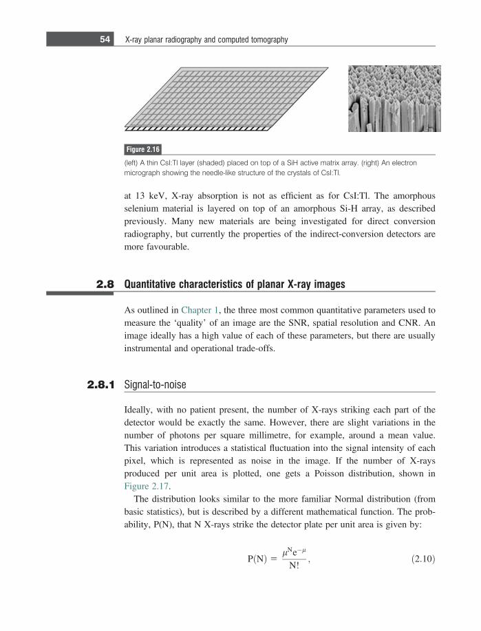
at 13 keV, X-ray absorption is not as efficient as for CsI:Tl. The amorphousselenium material is layered on top of an amorphous Si-H array, as describedpreviously. Many new materials are being investigated for direct conversionradiography, but currently the properties of the indirect-conversion detectors aremore favourable.
2.8 Quantitative characteristics of planar X-ray images
As outlined in Chapter 1, the three most common quantitative parameters used tomeasure the ‘quality’ of an image are the SNR, spatial resolution and CNR. Animage ideally has a high value of each of these parameters, but there are usuallyinstrumental and operational trade-offs.
2.8.1 Signal-to-noise
Ideally, with no patient present, the number of X-rays striking each part of thedetector would be exactly the same. However, there are slight variations in thenumber of photons per square millimetre, for example, around a mean value.This variation introduces a statistical fluctuation into the signal intensity of eachpixel, which is represented as noise in the image. If the number of X-raysproduced per unit area is plotted, one gets a Poisson distribution, shown inFigure 2.17.
The distribution looks similar to the more familiar Normal distribution (frombasic statistics), but is described by a different mathematical function. The prob-ability, P(N), that N X-rays strike the detector plate per unit area is given by:
P Nð Þ 5lNe�l
N!; ð2:10Þ
Figure 2.16
(left) A thin CsI:Tl layer (shaded) placed on top of a SiH active matrix array. (right) An electronmicrograph showing the needle-like structure of the crystals of CsI:Tl.
54 X-ray planar radiography and computed tomography
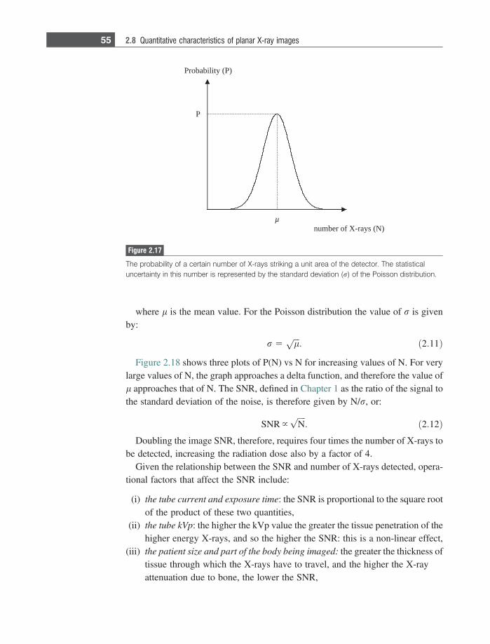
where l is the mean value. For the Poisson distribution the value of r is givenby:
r 5ffiffiffilp
: ð2:11Þ
Figure 2.18 shows three plots of P(N) vs N for increasing values of N. For verylarge values of N, the graph approaches a delta function, and therefore the value ofl approaches that of N. The SNR, defined in Chapter 1 as the ratio of the signal tothe standard deviation of the noise, is therefore given by N/r, or:
SNR }ffiffiffiffiNp
: ð2:12ÞDoubling the image SNR, therefore, requires four times the number of X-rays to
be detected, increasing the radiation dose also by a factor of 4.Given the relationship between the SNR and number of X-rays detected, opera-
tional factors that affect the SNR include:
(i) the tube current and exposure time: the SNR is proportional to the square rootof the product of these two quantities,
(ii) the tube kVp: the higher the kVp value the greater the tissue penetration of thehigher energy X-rays, and so the higher the SNR: this is a non-linear effect,
(iii) the patient size and part of the body being imaged: the greater the thickness oftissue through which the X-rays have to travel, and the higher the X-rayattenuation due to bone, the lower the SNR,
Probability (P)
P
µnumber of X-rays (N)
Figure 2.17
The probability of a certain number of X-rays striking a unit area of the detector. The statisticaluncertainty in this number is represented by the standard deviation (r) of the Poisson distribution.
55 2.8 Quantitative characteristics of planar X-ray images
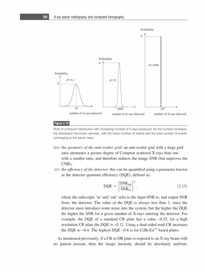
(iv) the geometry of the anti-scatter grid: an anti-scatter grid with a large gridratio attenuates a greater degree of Compton scattered X-rays than onewith a smaller ratio, and therefore reduces the image SNR (but improves theCNR),
(v) the efficiency of the detector: this can be quantified using a parameter knownas the detector quantum efficiency (DQE), defined as:
DQE 5SNRout
SNRin
� �2
; ð2:13Þ
where the subscripts ‘in’ and ‘out’ refer to the input SNR to, and output SNRfrom, the detector. The value of the DQE is always less than 1, since thedetector must introduce some noise into the system, but the higher the DQEthe higher the SNR for a given number of X-rays entering the detector. Forexample, the DQE of a standard CR plate has a value ~0.25, for a highresolution CR plate the DQE is ~0.12. Using a dual-sided read CR increasesthe DQE to ~0.4. The highest DQE ~0.8 is for CsBr:Eu2+ based plates.
As mentioned previously, if a CR or DR plate is exposed to an X-ray beam withno patient present, then the image intensity should be absolutely uniform.
ProbabilityP
1000
number of X-rays detected
σ =31
Probability
P
10
number of X-rays detected
σ =3.1
Probability
P
106
number of X-rays detected
σ =1000
Figure 2.18
Plots of a Poisson distribution with increasing number of X-rays produced. As the number increases,the distribution becomes narrower, with the mean number of events and the total number of eventsconverging to the same value.
56 X-ray planar radiography and computed tomography
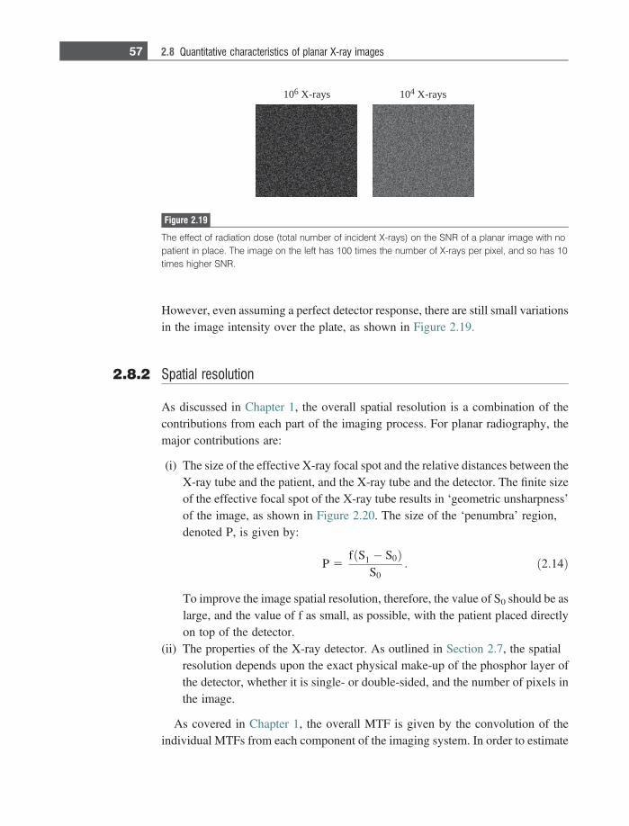
However, even assuming a perfect detector response, there are still small variationsin the image intensity over the plate, as shown in Figure 2.19.
2.8.2 Spatial resolution
As discussed in Chapter 1, the overall spatial resolution is a combination of thecontributions from each part of the imaging process. For planar radiography, themajor contributions are:
(i) The size of the effective X-ray focal spot and the relative distances between theX-ray tube and the patient, and the X-ray tube and the detector. The finite sizeof the effective focal spot of the X-ray tube results in ‘geometric unsharpness’of the image, as shown in Figure 2.20. The size of the ‘penumbra’ region,denoted P, is given by:
P 5fðS1 � S0Þ
S0: ð2:14Þ
To improve the image spatial resolution, therefore, the value of S0 should be aslarge, and the value of f as small, as possible, with the patient placed directlyon top of the detector.
(ii) The properties of the X-ray detector. As outlined in Section 2.7, the spatialresolution depends upon the exact physical make-up of the phosphor layer ofthe detector, whether it is single- or double-sided, and the number of pixels inthe image.
As covered in Chapter 1, the overall MTF is given by the convolution of theindividual MTFs from each component of the imaging system. In order to estimate
106 X-rays 104 X-rays
Figure 2.19
The effect of radiation dose (total number of incident X-rays) on the SNR of a planar image with nopatient in place. The image on the left has 100 times the number of X-rays per pixel, and so has 10times higher SNR.
57 2.8 Quantitative characteristics of planar X-ray images
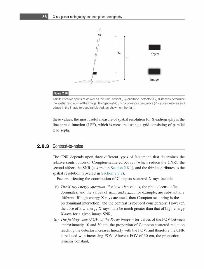
these values, the most useful measure of spatial resolution for X-radiography is theline spread function (LSF), which is measured using a grid consisting of parallellead septa.
2.8.3 Contrast-to-noise
The CNR depends upon three different types of factor: the first determines therelative contribution of Compton-scattered X-rays (which reduce the CNR), thesecond affects the SNR (covered in Section 2.8.1), and the third contributes to thespatial resolution (covered in Section 2.8.2).
Factors affecting the contribution of Compton-scattered X-rays include:
(i) The X-ray energy spectrum. For low kVp values, the photoelectric effectdominates, and the values of lbone and ltissue, for example, are substantiallydifferent. If high energy X-rays are used, then Compton scattering is thepredominant interaction, and the contrast is reduced considerably. However,the dose of low-energy X-rays must be much greater than that of high-energyX-rays for a given image SNR,
(ii) The field-of-view (FOV) of the X-ray image – for values of the FOV betweenapproximately 10 and 30 cm, the proportion of Compton scattered radiationreaching the detector increases linearly with the FOV, and therefore the CNRis reduced with increasing FOV. Above a FOV of 30 cm, the proportionremains constant,
f
S0S1
p
object
image
Figure 2.20
A finite effective spot size as well as the tube–patient (S0) and tube–detector (S1) distances determinethe spatial resolution of the image. The ‘geometric unsharpness’ or penumbra (P) causes features andedges in the image to become blurred, as shown on the right.
58 X-ray planar radiography and computed tomography
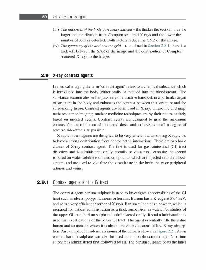
(iii) The thickness of the body part being imaged – the thicker the section, then thelarger the contribution from Compton scattered X-rays and the lower thenumber of X-rays detected. Both factors reduce the CNR of the image,
(iv) The geometry of the anti-scatter grid – as outlined in Section 2.8.1, there is atrade-off between the SNR of the image and the contribution of Comptonscattered X-rays to the image.
2.9 X-ray contrast agents
In medical imaging the term ‘contrast agent’ refers to a chemical substance whichis introduced into the body (either orally or injected into the bloodstream). Thesubstance accumulates, either passively or via active transport, in a particular organor structure in the body and enhances the contrast between that structure and thesurrounding tissue. Contrast agents are often used in X-ray, ultrasound and mag-netic resonance imaging: nuclear medicine techniques are by their nature entirelybased on injected agents. Contrast agents are designed to give the maximumcontrast for the minimum administered dose, and to have as small a degree ofadverse side-effects as possible.
X-ray contrast agents are designed to be very efficient at absorbing X-rays, i.e.to have a strong contribution from photoelectric interactions. There are two basicclasses of X-ray contrast agent. The first is used for gastrointestinal (GI) tractdisorders and is administered orally, rectally or via a nasal cannula: the secondis based on water-soluble iodinated compounds which are injected into the blood-stream, and are used to visualize the vasculature in the brain, heart or peripheralarteries and veins.
2.9.1 Contrast agents for the GI tract
The contrast agent barium sulphate is used to investigate abnormalities of the GItract such as ulcers, polyps, tumours or hernias. Barium has a K-edge at 37.4 keV,and so is a very efficient absorber of X-rays. Barium sulphate is a powder, which isprepared for patient administration as a thick suspension in water. For studies ofthe upper GI tract, barium sulphate is administered orally. Rectal administration isused for investigations of the lower GI tract. The agent essentially fills the entirelumen and so areas in which it is absent are visible as areas of low X-ray absorp-tion. An example of an adenocarcinoma of the colon is shown in Figure 2.21. As anenema, barium sulphate can also be used as a ‘double contrast agent’: bariumsulphate is administered first, followed by air. The barium sulphate coats the inner
59 2.9 X-ray contrast agents
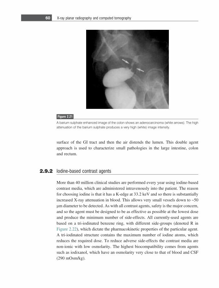
surface of the GI tract and then the air distends the lumen. This double agentapproach is used to characterize small pathologies in the large intestine, colonand rectum.
2.9.2 Iodine-based contrast agents
More than 40 million clinical studies are performed every year using iodine-basedcontrast media, which are administered intravenously into the patient. The reasonfor choosing iodine is that it has a K-edge at 33.2 keV and so there is substantiallyincreased X-ray attenuation in blood. This allows very small vessels down to ~50lm diameter to be detected. As with all contrast agents, safety is the major concern,and so the agent must be designed to be as effective as possible at the lowest doseand produce the minimum number of side-effects. All currently-used agents arebased on a tri-iodinated benzene ring, with different side-groups (denoted R inFigure 2.22), which dictate the pharmacokinetic properties of the particular agent.A tri-iodinated structure contains the maximum number of iodine atoms, whichreduces the required dose. To reduce adverse side-effects the contrast media arenon-ionic with low osmolarity. The highest biocompatibility comes from agentssuch as iodixanol, which have an osmolarity very close to that of blood and CSF(290 mOsm/kg).
Figure 2.21
A barium sulphate enhanced image of the colon shows an adenocarcinoma (white arrows). The highattenuation of the barium sulphate produces a very high (white) image intensity.
60 X-ray planar radiography and computed tomography
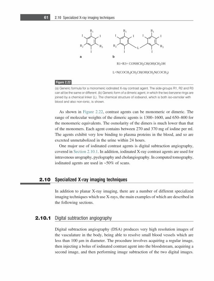
As shown in Figure 2.22, contrast agents can be monomeric or dimeric. Therange of molecular weights of the dimeric agents is 1300–1600, and 650–800 forthe monomeric equivalents. The osmolarity of the dimers is much lower than thatof the monomers. Each agent contains between 270 and 370 mg of iodine per ml.The agents exhibit very low binding to plasma proteins in the blood, and so areexcreted unmetabolized in the urine within 24 hours.
One major use of iodinated contrast agents is digital subtraction angiography,covered in Section 2.10.1. In addition, iodinated X-ray contrast agents are used forintravenous urography, pyelography and cholangiography. In computed tomography,iodinated agents are used in ~50% of scans.
2.10 Specialized X-ray imaging techniques
In addition to planar X-ray imaging, there are a number of different specializedimaging techniques which use X-rays, the main examples of which are described inthe following sections.
2.10.1 Digital subtraction angiography
Digital subtraction angiography (DSA) produces very high resolution images ofthe vasculature in the body, being able to resolve small blood vessels which areless than 100 lm in diameter. The procedure involves acquiring a regular image,then injecting a bolus of iodinated contrast agent into the bloodstream, acquiring asecond image, and then performing image subtraction of the two digital images.
I
R2
I
I
R1
R3
L=N(COCH3)CH2CH(OH)CH2N(COCH3)
I
R2
I
I
R1
II
I
R1
R3L
R1=R3= CONHCH2CH(OH)CH2OH
ba
Figure 2.22
(a) Generic formula for a monomeric iodinated X-ray contrast agent. The side-groups R1, R2 and R3can all be the same or different. (b) Generic form of a dimeric agent, in which the two benzene rings arejoined by a chemical linker (L). The chemical structure of iodixanol, which is both iso-osmolar withblood and also non-ionic, is shown.
61 2.10 Specialized X-ray imaging techniques
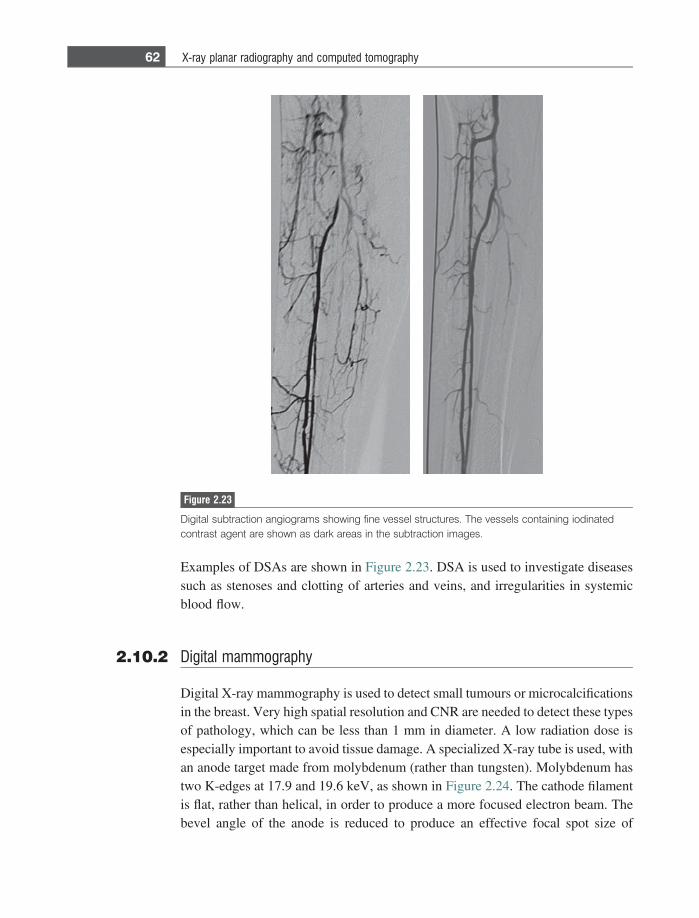
Examples of DSAs are shown in Figure 2.23. DSA is used to investigate diseasessuch as stenoses and clotting of arteries and veins, and irregularities in systemicblood flow.
2.10.2 Digital mammography
Digital X-ray mammography is used to detect small tumours or microcalcificationsin the breast. Very high spatial resolution and CNR are needed to detect these typesof pathology, which can be less than 1 mm in diameter. A low radiation dose isespecially important to avoid tissue damage. A specialized X-ray tube is used, withan anode target made from molybdenum (rather than tungsten). Molybdenum hastwo K-edges at 17.9 and 19.6 keV, as shown in Figure 2.24. The cathode filamentis flat, rather than helical, in order to produce a more focused electron beam. Thebevel angle of the anode is reduced to produce an effective focal spot size of
Figure 2.23
Digital subtraction angiograms showing fine vessel structures. The vessels containing iodinatedcontrast agent are shown as dark areas in the subtraction images.
62 X-ray planar radiography and computed tomography
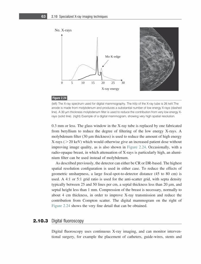
0.3 mm or less. The glass window in the X-ray tube is replaced by one fabricatedfrom beryllium to reduce the degree of filtering of the low energy X-rays. Amolybdenum filter (30 lm thickness) is used to reduce the amount of high energyX-rays (.20 keV) which would otherwise give an increased patient dose withoutimproving image quality, as is also shown in Figure 2.24. Occasionally, with aradio-opaque breast, in which attenuation of X-rays is particularly high, an alumi-nium filter can be used instead of molybdenum.
As described previously, the detector can either be CR or DR-based. The highestspatial resolution configuration is used in either case. To reduce the effects ofgeometric unsharpness, a large focal-spot-to-detector distance (45 to 80 cm) isused. A 4:1 or 5:1 grid ratio is used for the anti-scatter grid, with septa densitytypically between 25 and 50 lines per cm, a septal thickness less than 20 lm, andseptal height less than 1 mm. Compression of the breast is necessary, normally toabout 4 cm thickness, in order to improve X-ray transmission and reduce thecontribution from Compton scatter. The digital mammogram on the right ofFigure 2.24 shows the very fine detail that can be obtained.
2.10.3 Digital fluoroscopy
Digital fluoroscopy uses continuous X-ray imaging, and can monitor interven-tional surgery, for example the placement of catheters, guide-wires, stents and
0 5 10 15 20 25 30
No. X-rays
X-ray energy
Mo K-edge
Figure 2.24
(left) The X-ray spectrum used for digital mammography. The kVp of the X-ray tube is 26 keV.Theanode is made from molybdenum and produces a substantial number of low energy X-rays (dashedline). A 30 lm thickness molybdenum filter is used to reduce the contribution from very low energy X-rays (solid line). (right) Example of a digital mammogram, showing very high spatial resolution.
63 2.10 Specialized X-ray imaging techniques
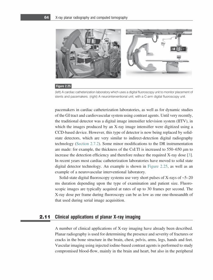
pacemakers in cardiac catheterization laboratories, as well as for dynamic studiesof the GI tract and cardiovascular system using contrast agents. Until very recently,the traditional detector was a digital image intensifier television system (IITV), inwhich the images produced by an X-ray image intensifier were digitized using aCCD-based device. However, this type of detector is now being replaced by solid-state detectors, which are very similar to indirect-detection digital radiographytechnology (Section 2.7.2). Some minor modifications to the DR instrumentationare made: for example, the thickness of the CsI:Tl is increased to 550–650 lm toincrease the detection efficiency and therefore reduce the required X-ray dose [3].In recent years most cardiac catheterization laboratories have moved to solid statedigital detector technology. An example is shown in Figure 2.25, as well as anexample of a neurovascular interventional laboratory.
Solid-state digital fluoroscopy systems use very short pulses of X-rays of ~5–20ms duration depending upon the type of examination and patient size. Fluoro-scopic images are typically acquired at rates of up to 30 frames per second. TheX-ray dose per frame during fluoroscopy can be as low as one one-thousandth ofthat used during serial image acquisition.
2.11 Clinical applications of planar X-ray imaging
A number of clinical applications of X-ray imaging have already been described.Planar radiography is used for determining the presence and severity of fractures orcracks in the bone structure in the brain, chest, pelvis, arms, legs, hands and feet.Vascular imaging using injected iodine-based contrast agents is performed to studycompromised blood-flow, mainly in the brain and heart, but also in the peripheral
Figure 2.25
(left) A cardiac catheterization laboratory which uses a digital fluoroscopy unit to monitor placement ofstents and pacemakers. (right) A neurointerventional unit, with a C-arm digital fluoroscopy unit.
64 X-ray planar radiography and computed tomography
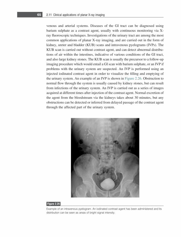
venous and arterial systems. Diseases of the GI tract can be diagnosed usingbarium sulphate as a contrast agent, usually with continuous monitoring via X-ray fluoroscopic techniques. Investigations of the urinary tract are among the mostcommon applications of planar X-ray imaging, and are carried out in the form ofkidney, ureter and bladder (KUB) scans and intravenous pyelograms (IVPs). TheKUB scan is carried out without contrast agent, and can detect abnormal distribu-tions of air within the intestines, indicative of various conditions of the GI tract,and also large kidney stones. The KUB scan is usually the precursor to a follow-upimaging procedure which would entail a GI scan with barium sulphate, or an IVP ifproblems with the urinary system are suspected. An IVP is performed using aninjected iodinated contrast agent in order to visualize the filling and emptying ofthe urinary system. An example of an IVP is shown in Figure 2.26. Obstruction tonormal flow through the system is usually caused by kidney stones, but can resultfrom infections of the urinary system. An IVP is carried out as a series of imagesacquired at different times after injection of the contrast agent. Normal excretion ofthe agent from the bloodstream via the kidneys takes about 30 minutes, but anyobstructions can be detected or inferred from delayed passage of the contrast agentthrough the affected part of the urinary system.
Figure 2.26
Example of an intravenous pyelogram. An iodinated contrast agent has been administered and itsdistribution can be seen as areas of bright signal intensity.
65 2.11 Clinical applications of planar X-ray imaging
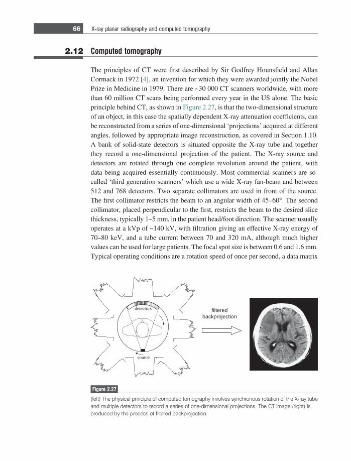
2.12 Computed tomography
The principles of CT were first described by Sir Godfrey Hounsfield and AllanCormack in 1972 [4], an invention for which they were awarded jointly the NobelPrize in Medicine in 1979. There are ~30 000 CT scanners worldwide, with morethan 60 million CT scans being performed every year in the US alone. The basicprinciple behind CT, as shown in Figure 2.27, is that the two-dimensional structureof an object, in this case the spatially dependent X-ray attenuation coefficients, canbe reconstructed from a series of one-dimensional ‘projections’ acquired at differentangles, followed by appropriate image reconstruction, as covered in Section 1.10.A bank of solid-state detectors is situated opposite the X-ray tube and togetherthey record a one-dimensional projection of the patient. The X-ray source anddetectors are rotated through one complete revolution around the patient, withdata being acquired essentially continuously. Most commercial scanners are so-called ‘third generation scanners’ which use a wide X-ray fan-beam and between512 and 768 detectors. Two separate collimators are used in front of the source.The first collimator restricts the beam to an angular width of 45–60�. The secondcollimator, placed perpendicular to the first, restricts the beam to the desired slicethickness, typically 1–5 mm, in the patient head/foot direction. The scanner usuallyoperates at a kVp of ~140 kV, with filtration giving an effective X-ray energy of70–80 keV, and a tube current between 70 and 320 mA, although much highervalues can be used for large patients. The focal spot size is between 0.6 and 1.6 mm.Typical operating conditions are a rotation speed of once per second, a data matrix
filteredbackprojection
source
detectors
Figure 2.27
(left) The physical principle of computed tomography involves synchronous rotation of the X-ray tubeand multiple detectors to record a series of one-dimensional projections. The CT image (right) isproduced by the process of filtered backprojection.
66 X-ray planar radiography and computed tomography
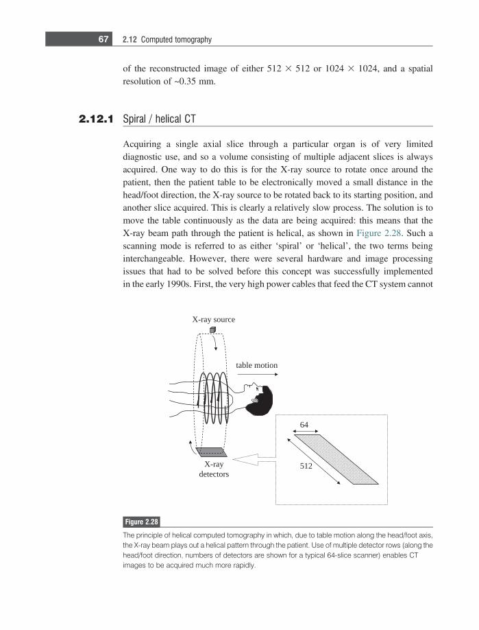
of the reconstructed image of either 512 3 512 or 1024 3 1024, and a spatialresolution of ~0.35 mm.
2.12.1 Spiral / helical CT
Acquiring a single axial slice through a particular organ is of very limiteddiagnostic use, and so a volume consisting of multiple adjacent slices is alwaysacquired. One way to do this is for the X-ray source to rotate once around thepatient, then the patient table to be electronically moved a small distance in thehead/foot direction, the X-ray source to be rotated back to its starting position, andanother slice acquired. This is clearly a relatively slow process. The solution is tomove the table continuously as the data are being acquired: this means that theX-ray beam path through the patient is helical, as shown in Figure 2.28. Such ascanning mode is referred to as either ‘spiral’ or ‘helical’, the two terms beinginterchangeable. However, there were several hardware and image processingissues that had to be solved before this concept was successfully implementedin the early 1990s. First, the very high power cables that feed the CT system cannot
X-ray source
X-raydetectors
512
64
table motion
Figure 2.28
The principle of helical computed tomography in which, due to table motion along the head/foot axis,the X-ray beam plays out a helical pattern through the patient. Use of multiple detector rows (along thehead/foot direction, numbers of detectors are shown for a typical 64-slice scanner) enables CTimages to be acquired much more rapidly.
67 2.12 Computed tomography

physically be rotated continuously in one direction, and similarly for the datatransfer cables attached to the detector bank. A ‘contactless’ method of bothdelivering power and receiving data had to be designed. Second, the X-ray tubeis effectively operating in continuous mode, and therefore the anode heating ismuch greater than for single-slice imaging. Finally, since the beam pattern throughthe patient is now helical rather than consisting of parallel projections, modifiedimage reconstruction algorithms had to be developed. The first ‘spiral CT’, devel-oped in the early 1990s, significantly reduced image acquisition times and enabledmuch greater volumes to be covered in a clinical scan.
In a helical scan, the pitch (p) is defined as the ratio of the table feed (d) perrotation of the X-ray tube to the collimated slice thickness (S):
p 5dS: ð2:15Þ
The value of p typically used in clinical scans lies between 1 and 2. Thereduction in tissue radiation dose, compared to an equivalent series of single-slicescans, is equal to the value of p.
2.12.2 Multi-slice spiral CT
The efficiency of spiral CT can be increased further by incorporating an array ofdetectors, rather than having just a single detector, in the head/foot direction. Suchan array is also shown in Figure 2.28. The increase in efficiency arises from thehigher values of the table feed per rotation that can be used. Multi-slice spiral CTcan be used to image larger volumes in a given time, or to image a given volume ina shorter scan time, compared to conventional spiral CT. The effective slice thick-ness is dictated by the dimensions of the individual detectors, rather than thecollimated X-ray beam width as is the case for a single detector, which allowsthinner slices to be acquired. Modern multi-detector CT (MDCT) systems have upto 256 or 320 detector rows.
2.13 Instrumentation for CT
Several components of the CT system such as the X-ray tube, collimator and anti-scatter grid are very similar to the instrumentation described previously for planarX-radiography. The tube and detectors have to be fixed to a heavy gantry, whichrotates very rapidly, generating large gravitational forces. High power cables areused to deliver power to the X-ray tube, and a large parallel cable is used to transfer
68 X-ray planar radiography and computed tomography
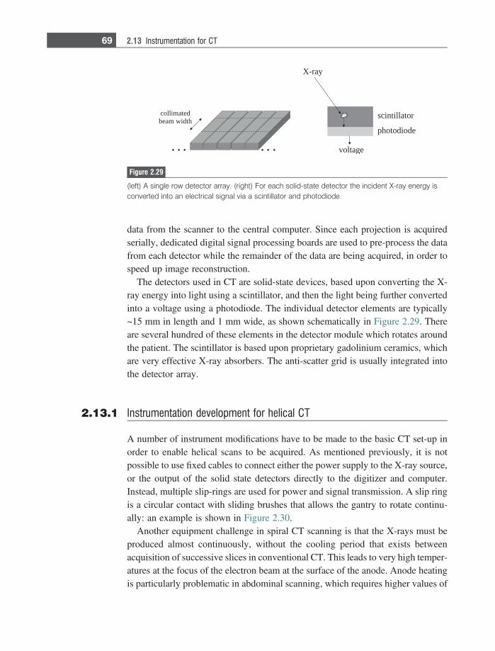
data from the scanner to the central computer. Since each projection is acquiredserially, dedicated digital signal processing boards are used to pre-process the datafrom each detector while the remainder of the data are being acquired, in order tospeed up image reconstruction.
The detectors used in CT are solid-state devices, based upon converting the X-ray energy into light using a scintillator, and then the light being further convertedinto a voltage using a photodiode. The individual detector elements are typically~15 mm in length and 1 mm wide, as shown schematically in Figure 2.29. Thereare several hundred of these elements in the detector module which rotates aroundthe patient. The scintillator is based upon proprietary gadolinium ceramics, whichare very effective X-ray absorbers. The anti-scatter grid is usually integrated intothe detector array.
2.13.1 Instrumentation development for helical CT
A number of instrument modifications have to be made to the basic CT set-up inorder to enable helical scans to be acquired. As mentioned previously, it is notpossible to use fixed cables to connect either the power supply to the X-ray source,or the output of the solid state detectors directly to the digitizer and computer.Instead, multiple slip-rings are used for power and signal transmission. A slip ringis a circular contact with sliding brushes that allows the gantry to rotate continu-ally: an example is shown in Figure 2.30.
Another equipment challenge in spiral CT scanning is that the X-rays must beproduced almost continuously, without the cooling period that exists betweenacquisition of successive slices in conventional CT. This leads to very high temper-atures at the focus of the electron beam at the surface of the anode. Anode heatingis particularly problematic in abdominal scanning, which requires higher values of
scintillator
photodiode
voltage
X-ray
collimatedbeam width
Figure 2.29
(left) A single row detector array. (right) For each solid-state detector the incident X-ray energy isconverted into an electrical signal via a scintillator and photodiode.
69 2.13 Instrumentation for CT
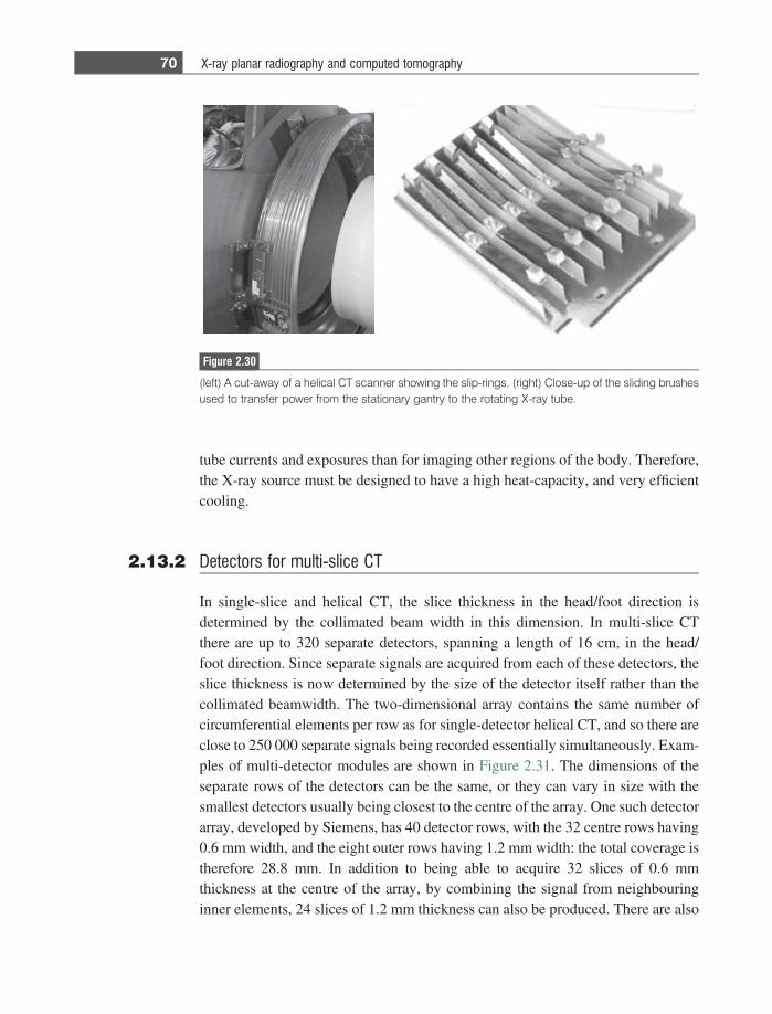
tube currents and exposures than for imaging other regions of the body. Therefore,the X-ray source must be designed to have a high heat-capacity, and very efficientcooling.
2.13.2 Detectors for multi-slice CT
In single-slice and helical CT, the slice thickness in the head/foot direction isdetermined by the collimated beam width in this dimension. In multi-slice CTthere are up to 320 separate detectors, spanning a length of 16 cm, in the head/foot direction. Since separate signals are acquired from each of these detectors, theslice thickness is now determined by the size of the detector itself rather than thecollimated beamwidth. The two-dimensional array contains the same number ofcircumferential elements per row as for single-detector helical CT, and so there areclose to 250 000 separate signals being recorded essentially simultaneously. Exam-ples of multi-detector modules are shown in Figure 2.31. The dimensions of theseparate rows of the detectors can be the same, or they can vary in size with thesmallest detectors usually being closest to the centre of the array. One such detectorarray, developed by Siemens, has 40 detector rows, with the 32 centre rows having0.6 mm width, and the eight outer rows having 1.2 mm width: the total coverage istherefore 28.8 mm. In addition to being able to acquire 32 slices of 0.6 mmthickness at the centre of the array, by combining the signal from neighbouringinner elements, 24 slices of 1.2 mm thickness can also be produced. There are also
Figure 2.30
(left) A cut-away of a helical CT scanner showing the slip-rings. (right) Close-up of the sliding brushesused to transfer power from the stationary gantry to the rotating X-ray tube.
70 X-ray planar radiography and computed tomography
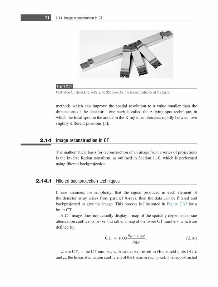
methods which can improve the spatial resolution to a value smaller than thedimensions of the detector – one such is called the z-flying spot technique, inwhich the focal spot on the anode in the X-ray tube alternates rapidly between twoslightly different positions [5].
2.14 Image reconstruction in CT
The mathematical basis for reconstruction of an image from a series of projectionsis the inverse Radon transform, as outlined in Section 1.10, which is performedusing filtered backprojection.
2.14.1 Filtered backprojection techniques
If one assumes, for simplicity, that the signal produced in each element ofthe detector array arises from parallel X-rays, then the data can be filtered andbackprojected to give the image. This process is illustrated in Figure 2.32 for abrain CT.
A CT image does not actually display a map of the spatially-dependent tissueattenuation coefficents per se, but rather a map of the tissue CT numbers, which aredefined by:
CTo 5 1000lo � lH2O
lH2O; ð2:16Þ
where CTo is the CT number, with values expressed in Hounsfield units (HU),and lo the linear attenuation coefficient of the tissue in each pixel. The reconstructed
Figure 2.31
Multi-slice CT detectors, with up to 320 rows for the largest detector at the back.
71 2.14 Image reconstruction in CT
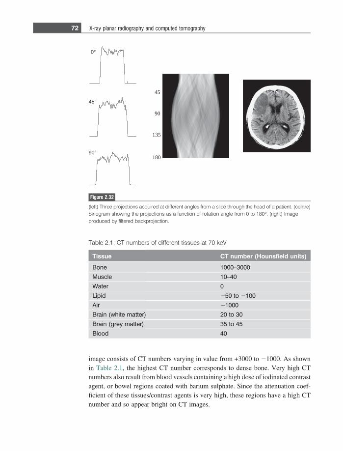
image consists of CT numbers varying in value from +3000 to 21000. As shownin Table 2.1, the highest CT number corresponds to dense bone. Very high CTnumbers also result from blood vessels containing a high dose of iodinated contrastagent, or bowel regions coated with barium sulphate. Since the attenuation coef-ficient of these tissues/contrast agents is very high, these regions have a high CTnumber and so appear bright on CT images.
45
90
180
135
0°
45°
90°
Figure 2.32
(left) Three projections acquired at different angles from a slice through the head of a patient. (centre)Sinogram showing the projections as a function of rotation angle from 0 to 180�. (right) Imageproduced by filtered backprojection.
Table 2.1: CT numbers of different tissues at 70 keV
Tissue CT number (Hounsfield units)
Bone 1000–3000
Muscle 10–40
Water 0
Lipid 250 to 2100
Air 21000
Brain (white matter) 20 to 30
Brain (grey matter) 35 to 45
Blood 40
72 X-ray planar radiography and computed tomography
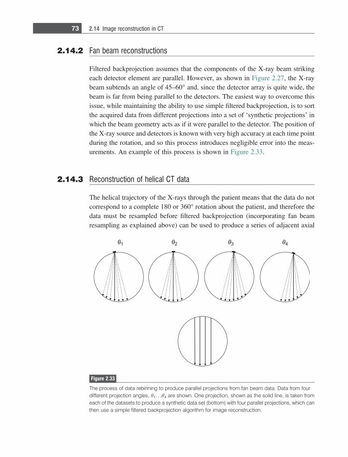
2.14.2 Fan beam reconstructions
Filtered backprojection assumes that the components of the X-ray beam strikingeach detector element are parallel. However, as shown in Figure 2.27, the X-raybeam subtends an angle of 45–60� and, since the detector array is quite wide, thebeam is far from being parallel to the detectors. The easiest way to overcome thisissue, while maintaining the ability to use simple filtered backprojection, is to sortthe acquired data from different projections into a set of ‘synthetic projections’ inwhich the beam geometry acts as if it were parallel to the detector. The position ofthe X-ray source and detectors is known with very high accuracy at each time pointduring the rotation, and so this process introduces negligible error into the meas-urements. An example of this process is shown in Figure 2.33.
2.14.3 Reconstruction of helical CT data
The helical trajectory of the X-rays through the patient means that the data do notcorrespond to a complete 180 or 360� rotation about the patient, and therefore thedata must be resampled before filtered backprojection (incorporating fan beamresampling as explained above) can be used to produce a series of adjacent axial
Figure 2.33
The process of data rebinning to produce parallel projections from fan beam data. Data from fourdifferent projection angles, h1. . .h4 are shown. One projection, shown as the solid line, is taken fromeach of the datasets to produce a synthetic data set (bottom) with four parallel projections, which canthen use a simple filtered backprojection algorithm for image reconstruction.
73 2.14 Image reconstruction in CT
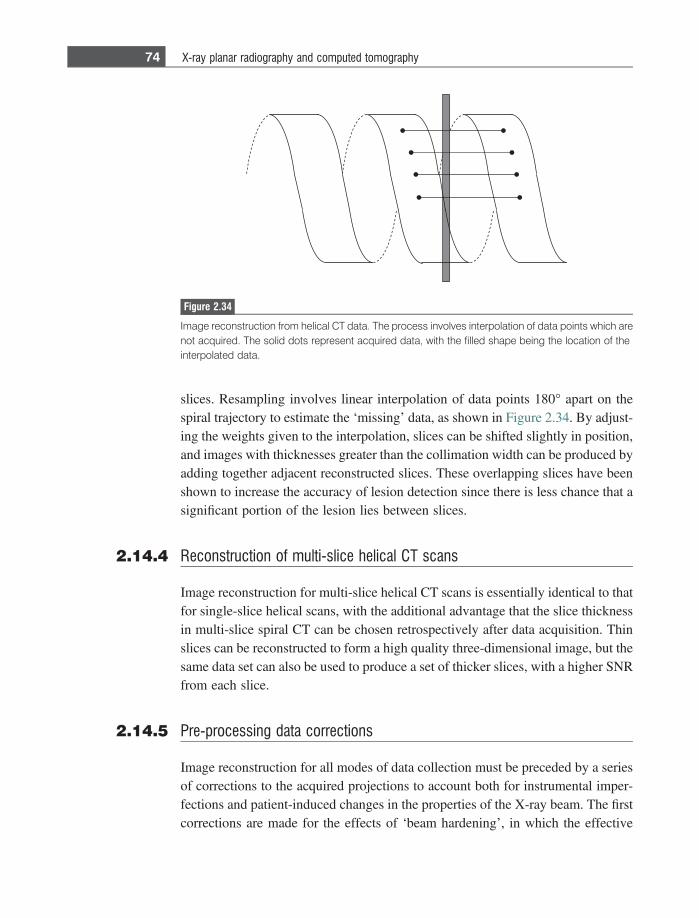
slices. Resampling involves linear interpolation of data points 180� apart on thespiral trajectory to estimate the ‘missing’ data, as shown in Figure 2.34. By adjust-ing the weights given to the interpolation, slices can be shifted slightly in position,and images with thicknesses greater than the collimation width can be produced byadding together adjacent reconstructed slices. These overlapping slices have beenshown to increase the accuracy of lesion detection since there is less chance that asignificant portion of the lesion lies between slices.
2.14.4 Reconstruction of multi-slice helical CT scans
Image reconstruction for multi-slice helical CT scans is essentially identical to thatfor single-slice helical scans, with the additional advantage that the slice thicknessin multi-slice spiral CT can be chosen retrospectively after data acquisition. Thinslices can be reconstructed to form a high quality three-dimensional image, but thesame data set can also be used to produce a set of thicker slices, with a higher SNRfrom each slice.
2.14.5 Pre-processing data corrections
Image reconstruction for all modes of data collection must be preceded by a seriesof corrections to the acquired projections to account both for instrumental imper-fections and patient-induced changes in the properties of the X-ray beam. The firstcorrections are made for the effects of ‘beam hardening’, in which the effective
Figure 2.34
Image reconstruction from helical CT data. The process involves interpolation of data points which arenot acquired. The solid dots represent acquired data, with the filled shape being the location of theinterpolated data.
74 X-ray planar radiography and computed tomography
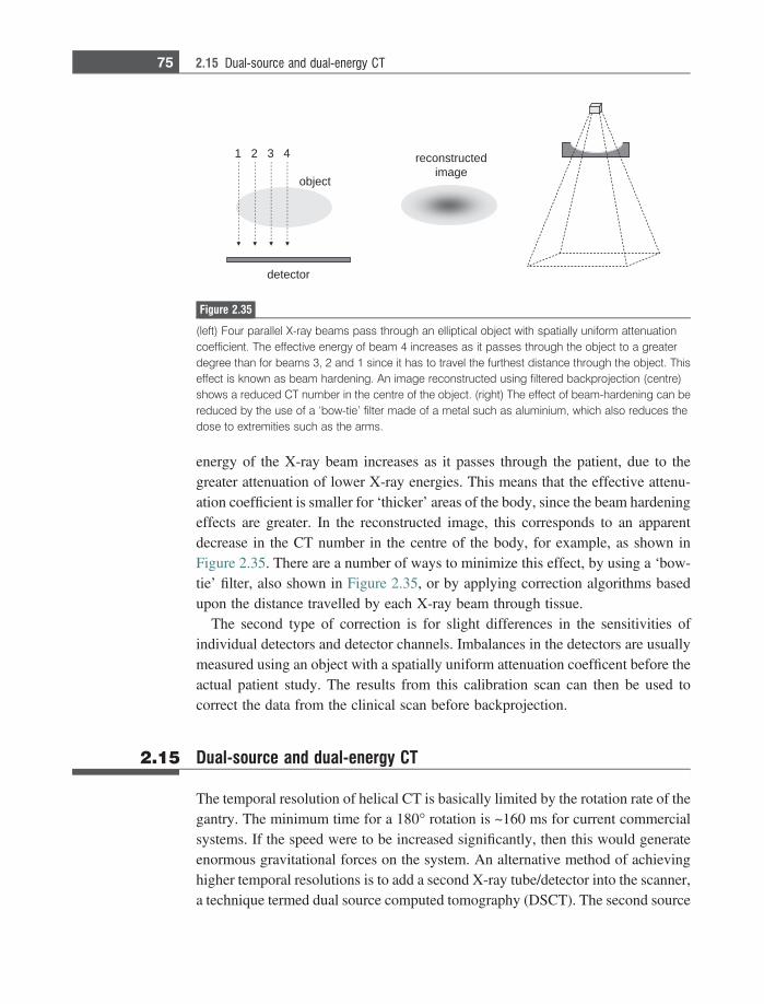
energy of the X-ray beam increases as it passes through the patient, due to thegreater attenuation of lower X-ray energies. This means that the effective attenu-ation coefficient is smaller for ‘thicker’ areas of the body, since the beam hardeningeffects are greater. In the reconstructed image, this corresponds to an apparentdecrease in the CT number in the centre of the body, for example, as shown inFigure 2.35. There are a number of ways to minimize this effect, by using a ‘bow-tie’ filter, also shown in Figure 2.35, or by applying correction algorithms basedupon the distance travelled by each X-ray beam through tissue.
The second type of correction is for slight differences in the sensitivities ofindividual detectors and detector channels. Imbalances in the detectors are usuallymeasured using an object with a spatially uniform attenuation coefficent before theactual patient study. The results from this calibration scan can then be used tocorrect the data from the clinical scan before backprojection.
2.15 Dual-source and dual-energy CT
The temporal resolution of helical CT is basically limited by the rotation rate of thegantry. The minimum time for a 180� rotation is ~160 ms for current commercialsystems. If the speed were to be increased significantly, then this would generateenormous gravitational forces on the system. An alternative method of achievinghigher temporal resolutions is to add a second X-ray tube/detector into the scanner,a technique termed dual source computed tomography (DSCT). The second source
4321
tcejbo
detcurtsnoceregami
rotceted
Figure 2.35
(left) Four parallel X-ray beams pass through an elliptical object with spatially uniform attenuationcoefficient. The effective energy of beam 4 increases as it passes through the object to a greaterdegree than for beams 3, 2 and 1 since it has to travel the furthest distance through the object. Thiseffect is known as beam hardening. An image reconstructed using filtered backprojection (centre)shows a reduced CT number in the centre of the object. (right) The effect of beam-hardening can bereduced by the use of a ‘bow-tie’ filter made of a metal such as aluminium, which also reduces thedose to extremities such as the arms.
75 2.15 Dual-source and dual-energy CT
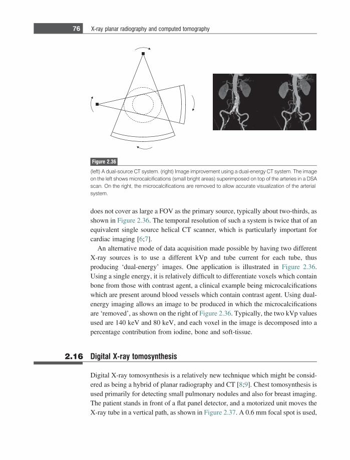
does not cover as large a FOV as the primary source, typically about two-thirds, asshown in Figure 2.36. The temporal resolution of such a system is twice that of anequivalent single source helical CT scanner, which is particularly important forcardiac imaging [6;7].
An alternative mode of data acquisition made possible by having two differentX-ray sources is to use a different kVp and tube current for each tube, thusproducing ‘dual-energy’ images. One application is illustrated in Figure 2.36.Using a single energy, it is relatively difficult to differentiate voxels which containbone from those with contrast agent, a clinical example being microcalcificationswhich are present around blood vessels which contain contrast agent. Using dual-energy imaging allows an image to be produced in which the microcalcificationsare ‘removed’, as shown on the right of Figure 2.36. Typically, the two kVp valuesused are 140 keV and 80 keV, and each voxel in the image is decomposed into apercentage contribution from iodine, bone and soft-tissue.
2.16 Digital X-ray tomosynthesis
Digital X-ray tomosynthesis is a relatively new technique which might be consid-ered as being a hybrid of planar radiography and CT [8;9]. Chest tomosynthesis isused primarily for detecting small pulmonary nodules and also for breast imaging.The patient stands in front of a flat panel detector, and a motorized unit moves theX-ray tube in a vertical path, as shown in Figure 2.37. A 0.6 mm focal spot is used,
Figure 2.36
(left) A dual-source CT system. (right) Image improvement using a dual-energy CT system. The imageon the left shows microcalcifications (small bright areas) superimposed on top of the arteries in a DSAscan. On the right, the microcalcifications are removed to allow accurate visualization of the arterialsystem.
76 X-ray planar radiography and computed tomography
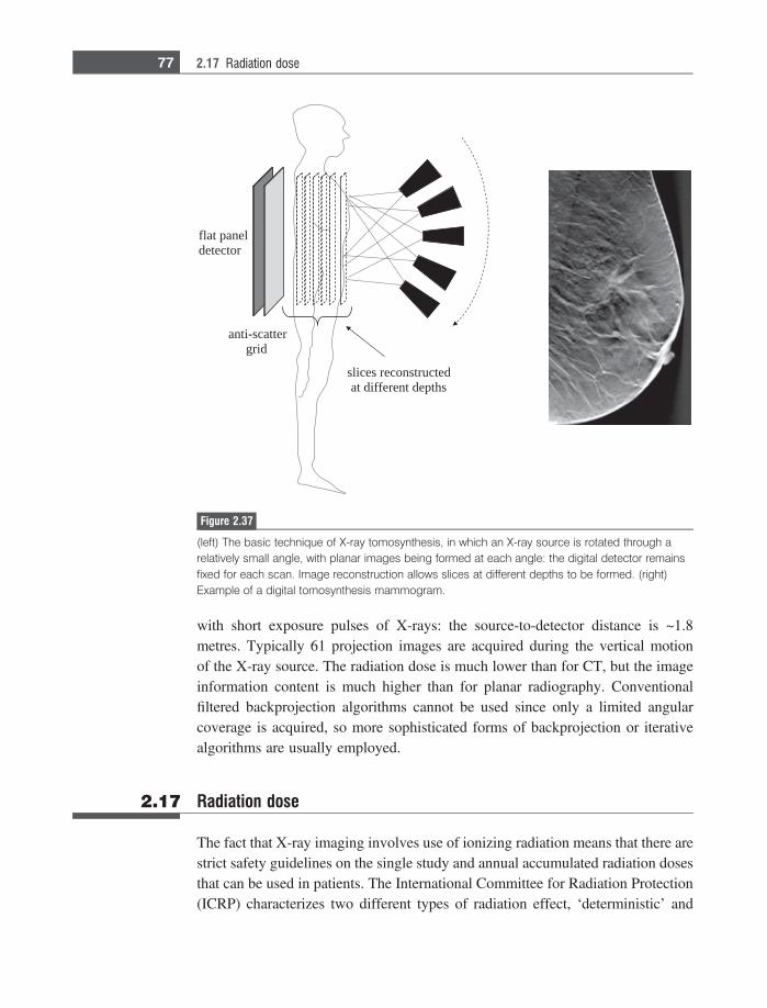
with short exposure pulses of X-rays: the source-to-detector distance is ~1.8metres. Typically 61 projection images are acquired during the vertical motionof the X-ray source. The radiation dose is much lower than for CT, but the imageinformation content is much higher than for planar radiography. Conventionalfiltered backprojection algorithms cannot be used since only a limited angularcoverage is acquired, so more sophisticated forms of backprojection or iterativealgorithms are usually employed.
2.17 Radiation dose
The fact that X-ray imaging involves use of ionizing radiation means that there arestrict safety guidelines on the single study and annual accumulated radiation dosesthat can be used in patients. The International Committee for Radiation Protection(ICRP) characterizes two different types of radiation effect, ‘deterministic’ and
flat paneldetector
anti-scattergrid
slices reconstructedat different depths
Figure 2.37
(left) The basic technique of X-ray tomosynthesis, in which an X-ray source is rotated through arelatively small angle, with planar images being formed at each angle: the digital detector remainsfixed for each scan. Image reconstruction allows slices at different depths to be formed. (right)Example of a digital tomosynthesis mammogram.
77 2.17 Radiation dose

‘stochastic’. Deterministic effects refer to cellular damage which leads to a loss intissue function if a sufficient number of cells are damaged. The probability of thishappening is very low at low radiation doses, but climbs steadily towards unitywith a dose above a certain threshold level. In contrast, stochastic effects refer tothe biological situation in which the cell is not killed, but genetic mutations causedby chromosomal damage lead, in time, to development of cancer. These stochasticeffects may occur at a much lower dose than deterministic effects: the higher thedose the greater the probability of cancer occurring, but importantly there is noabsolute threshold level. Given that the deterministic threshold limits are far abovethe doses encountered in normal X-ray procedures, the greatest concern is stochasticeffects.
Quantitatively, the absorbed dose (D) is defined as the radiation energy (E),measured in Joules, absorbed per kg of tissue. The value of D is given in units ofgrays (Gy), where 1 Gy equals 1 Joule/kg. The equivalent dose (HT) in a tissue isgiven by:
HT 5 +R
wRDT;R; ð2:17Þ
where
DT;R 51
mT
ðmT
DRdm: ð2:18Þ
Note that DT,R is the mean absorbed dose in tissue (T) with mass (mT) from agiven amount of radiation R, and wR is the radiation weighting factor (with a valueof 1 for both X-rays and c-rays). The unit of HT is J/kg, but it is typically reportedin sieverts (Sv), or millesieverts for realistic doses.
Some tissues are more sensitive to radiation damage than others, and this istaken into account by calculating the effective dose (E), which is given by thetissue equivalent dose weighted by the tissue weighting factor (wT) of that organ:
E 5 +T
wTHT: ð2:19Þ
Values of wT for different tissues are given in Table 2.2 with the number definedon a scale such that:
+T
wT 5 1: ð2:20Þ
The values of wT represent the fraction of the total stochastic radiation risk forall the different organs and tissue. For the gonads, which have the highest risk, this
78 X-ray planar radiography and computed tomography
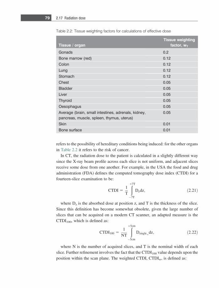
refers to the possibility of hereditary conditions being induced: for the other organsin Table 2.2 it refers to the risk of cancer.
In CT, the radiation dose to the patient is calculated in a slightly different waysince the X-ray beam profile across each slice is not uniform, and adjacent slicesreceive some dose from one another. For example, in the USA the food and drugadministration (FDA) defines the computed tomography dose index (CTDI) for afourteen-slice examination to be:
CTDI 51T
ð17T
�7T
Dzdz; ð2:21Þ
where Dz is the absorbed dose at position z, and T is the thickness of the slice.Since this definition has become somewhat obsolete, given the large number ofslices that can be acquired on a modern CT scanner, an adapted measure is theCTDI100, which is defined as:
CTDI100 51
NT
ðþ5cm
�5cm
Dsingle;z dz; ð2:22Þ
where N is the number of acquired slices, and T is the nominal width of eachslice. Further refinement involves the fact that the CTDI100 value depends upon theposition within the scan plane. The weighted CTDI, CTDIw, is defined as:
Table 2.2: Tissue weighting factors for calculations of effective dose
Tissue / organTissue weighting
factor, wT
Gonads 0.2
Bone marrow (red) 0.12
Colon 0.12
Lung 0.12
Stomach 0.12
Chest 0.05
Bladder 0.05
Liver 0.05
Thyroid 0.05
Oesophagus 0.05
Average (brain, small intestines, adrenals, kidney,pancreas, muscle, spleen, thymus, uterus)
0.05
Skin 0.01
Bone surface 0.01
79 2.17 Radiation dose
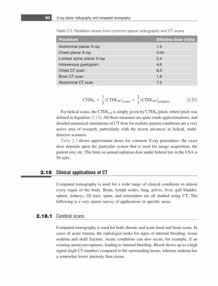
CTDIw 513
CTDI100ð Þcentre 123
CTDI100ð Þperiphery: ð2:23Þ
For helical scans, the CTDIvol is simply given by CTDIw/pitch, where pitch wasdefined in Equation (2.15). All these measures are quite crude approximations, anddetailed numerical simulations of CT dose for realistic patient conditions are a veryactive area of research, particularly with the recent advances in helical, multi-detector scanners.
Table 2.3 shows approximate doses for common X-ray procedures: the exactdose depends upon the particular system that is used for image acquisition, thepatient size, etc. The limit on annual radiation dose under federal law in the USA is50 mSv.
2.18 Clinical applications of CT
Computed tomography is used for a wide range of clinical conditions in almostevery organ of the body. Brain, lymph nodes, lung, pelvis, liver, gall bladder,spleen, kidneys, GI tract, spine, and extremities are all studied using CT. Thefollowing is a very sparse survey of applications in specific areas.
2.18.1 Cerebral scans
Computed tomography is used for both chronic and acute head and brain scans. Incases of acute trauma, the radiologist looks for signs of internal bleeding, tissueoedema and skull fracture. Acute conditions can also occur, for example, if anexisting aneurysm ruptures, leading to internal bleeding. Blood shows up as a highsignal (high CT number) compared to the surrounding tissue, whereas oedema hasa somewhat lower intensity than tissue.
Table 2.3: Radiation doses from common planar radiography and CT scans
Procedure Effective dose (mSv)
Abdominal planar X-ray 1.5
Chest planar X-ray 0.04
Lumbar spine planar X-ray 2.4
Intravenous pyelogram 4.6
Chest CT scan 8.3
Brain CT scan 1.8
Abdominal CT scan 7.2
80 X-ray planar radiography and computed tomography
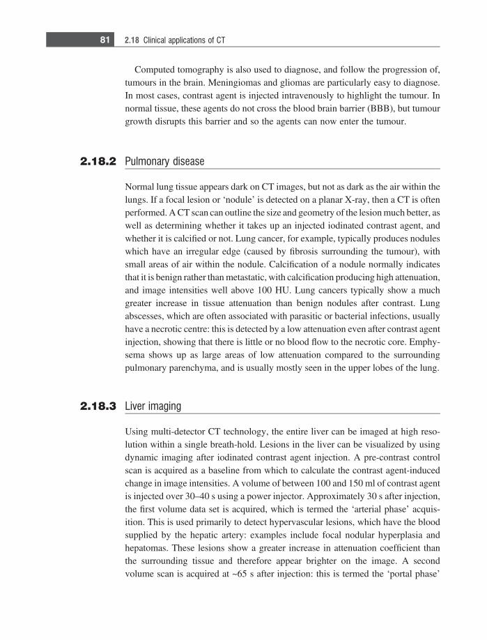
Computed tomography is also used to diagnose, and follow the progression of,tumours in the brain. Meningiomas and gliomas are particularly easy to diagnose.In most cases, contrast agent is injected intravenously to highlight the tumour. Innormal tissue, these agents do not cross the blood brain barrier (BBB), but tumourgrowth disrupts this barrier and so the agents can now enter the tumour.
2.18.2 Pulmonary disease
Normal lung tissue appears dark on CT images, but not as dark as the air within thelungs. If a focal lesion or ‘nodule’ is detected on a planar X-ray, then a CT is oftenperformed. A CT scan can outline the size and geometry of the lesion much better, aswell as determining whether it takes up an injected iodinated contrast agent, andwhether it is calcified or not. Lung cancer, for example, typically produces noduleswhich have an irregular edge (caused by fibrosis surrounding the tumour), withsmall areas of air within the nodule. Calcification of a nodule normally indicatesthat it is benign rather than metastatic, with calcification producing high attenuation,and image intensities well above 100 HU. Lung cancers typically show a muchgreater increase in tissue attenuation than benign nodules after contrast. Lungabscesses, which are often associated with parasitic or bacterial infections, usuallyhave a necrotic centre: this is detected by a low attenuation even after contrast agentinjection, showing that there is little or no blood flow to the necrotic core. Emphy-sema shows up as large areas of low attenuation compared to the surroundingpulmonary parenchyma, and is usually mostly seen in the upper lobes of the lung.
2.18.3 Liver imaging
Using multi-detector CT technology, the entire liver can be imaged at high reso-lution within a single breath-hold. Lesions in the liver can be visualized by usingdynamic imaging after iodinated contrast agent injection. A pre-contrast controlscan is acquired as a baseline from which to calculate the contrast agent-inducedchange in image intensities. A volume of between 100 and 150 ml of contrast agentis injected over 30–40 s using a power injector. Approximately 30 s after injection,the first volume data set is acquired, which is termed the ‘arterial phase’ acquis-ition. This is used primarily to detect hypervascular lesions, which have the bloodsupplied by the hepatic artery: examples include focal nodular hyperplasia andhepatomas. These lesions show a greater increase in attenuation coefficient thanthe surrounding tissue and therefore appear brighter on the image. A secondvolume scan is acquired at ~65 s after injection: this is termed the ‘portal phase’
81 2.18 Clinical applications of CT
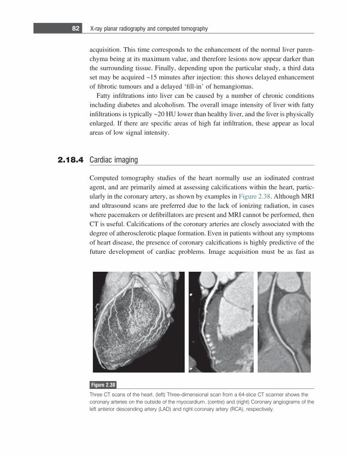
acquisition. This time corresponds to the enhancement of the normal liver paren-chyma being at its maximum value, and therefore lesions now appear darker thanthe surrounding tissue. Finally, depending upon the particular study, a third dataset may be acquired ~15 minutes after injection: this shows delayed enhancementof fibrotic tumours and a delayed ‘fill-in’ of hemangiomas.
Fatty infiltrations into liver can be caused by a number of chronic conditionsincluding diabetes and alcoholism. The overall image intensity of liver with fattyinfiltrations is typically ~20 HU lower than healthy liver, and the liver is physicallyenlarged. If there are specific areas of high fat infiltration, these appear as localareas of low signal intensity.
2.18.4 Cardiac imaging
Computed tomography studies of the heart normally use an iodinated contrastagent, and are primarily aimed at assessing calcifications within the heart, partic-ularly in the coronary artery, as shown by examples in Figure 2.38. Although MRIand ultrasound scans are preferred due to the lack of ionizing radiation, in caseswhere pacemakers or defibrillators are present and MRI cannot be performed, thenCT is useful. Calcifications of the coronary arteries are closely associated with thedegree of atherosclerotic plaque formation. Even in patients without any symptomsof heart disease, the presence of coronary calcifications is highly predictive of thefuture development of cardiac problems. Image acquisition must be as fast as
Figure 2.38
Three CT scans of the heart. (left) Three-dimensional scan from a 64-slice CT scanner shows thecoronary arteries on the outside of the myocardium. (centre) and (right) Coronary angiograms of theleft anterior descending artery (LAD) and right coronary artery (RCA), respectively.
82 X-ray planar radiography and computed tomography

possible to ‘freeze’ the cardiac motion and acquire all the projections within asingle breath-hold if possible: image acquisition is gated to the heart motion via anECG trigger. Although CT angiography is not a routine clinical procedure, it isvery useful to rule out coronary stenoses in patients with a predisposition to thedisease, and is highly informative in patients with a known or suspected congenitalartery anomaly.
Exercises
The X-ray energy spectrum2.1 Plot the energy spectra from a tungsten tube with the following kVp values:
120 keV, 80 keV, 60 keV and 40 keV.2.2 (a) Calculate the total number of electrons bombarding the target of an X-ray
tube operated at 100 mA for 0.1 seconds.(b) Calculate the maximum energy and minimum wavelength for an X-ray
beam generated at 110 kVp.2.3 The spectrum of X-ray energies changes as the X-rays pass through tissue
due to the energy dependence of the linear attenuation coefficient: this is aphenomenon known as beam hardening. A typical energy distribution of thebeam from the X-ray source is shown in Figure 2.6. Sketch the energyspectrum after the beam has passed through the body.
2.4 Look up the exact binding energies of the L and M shell electrons in tung-sten. Plot the exact distribution of characteristic energy lines that are pro-duced based upon these binding energies.
2.5 Two X-ray images of the hand are shown in Figure 2.39. One corresponds toan X-ray beam with an effective energy of 140 keV and the other to an
a b
Figure 2.39
See Exercise 2.5.
83 Exercises

effective energy of 50 keV. Explain which is which, and the reasons for thedifferences in image contrast and signal intensity.
2.6 Planar X-rays of a horse’s leg are shown in Figure 2.40. In (a), the kVp andtube current (mA) are chosen to give high contrast between the bone andsurrounding tissue. Explain how the kVp and mA settings would have to bechanged (increased, decreased, remain constant) to give the images shown in(b) and (c).
2.7 Starting from Equation (2.4) derive both Equations (2.5) and (2.6).
Linear and mass attenuation coefficients2.8 Show two mechanisms involving scattering in the body which allow Compton
scattered X-rays to be detected despite the presence of an anti-scattering grid.2.9 In Figure 2.41 calculate the X-ray intensity, as a function of the incident
intensity I0, that reaches the detector for each of the three X-ray beams. Thedark-shaded area represents bone, and the light-shaded area represents tissue.The linear attenuation coefficients at the effective X-ray energy of 68 keV are10 cm21 and 1 cm21 for bone and tissue, respectively.
2.10 The linear attenuation coefficient of a gadolinium-based phosphor used fordetection of X-rays is 560 cm21 at an X-ray energy of 150 keV. Whatpercentage of X-rays are detected by phosphor layers of 10 lm, 25 lm,and 50 lm thickness? What are the trade-offs in terms of spatial resolution?
X-ray detectors2.11 An X-ray with energy 60 keV strikes a gadolinium-based phosphor on a CR
plate producing photons at a wavelength of 415 nm. The energy conversioncoefficient for this process is 20%. How many photons are produced foreach incident X-ray? (Planck’s constant = 6.6331034 Js, 1 eV=1.6023
10219J).2.12 An X-ray is Compton scattered by an angle h at a distance z from the top of
the anti-scatter grid. Using simple geometry, calculate the maximum value ofh for a given grid ratio h/d that results in the X-ray being detected.
a b c
Figure 2.40
See Exercise 2.6.
84 X-ray planar radiography and computed tomography
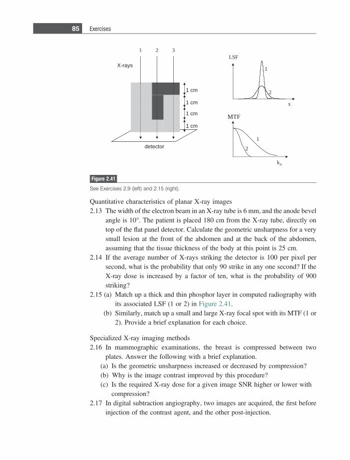
Quantitative characteristics of planar X-ray images2.13 The width of the electron beam in an X-ray tube is 6 mm, and the anode bevel
angle is 10�. The patient is placed 180 cm from the X-ray tube, directly ontop of the flat panel detector. Calculate the geometric unsharpness for a verysmall lesion at the front of the abdomen and at the back of the abdomen,assuming that the tissue thickness of the body at this point is 25 cm.
2.14 If the average number of X-rays striking the detector is 100 per pixel persecond, what is the probability that only 90 strike in any one second? If theX-ray dose is increased by a factor of ten, what is the probability of 900striking?
2.15 (a) Match up a thick and thin phosphor layer in computed radiography withits associated LSF (1 or 2) in Figure 2.41.
(b) Similarly, match up a small and large X-ray focal spot with its MTF (1 or2). Provide a brief explanation for each choice.
Specialized X-ray imaging methods2.16 In mammographic examinations, the breast is compressed between two
plates. Answer the following with a brief explanation.(a) Is the geometric unsharpness increased or decreased by compression?(b) Why is the image contrast improved by this procedure?(c) Is the required X-ray dose for a given image SNR higher or lower with
compression?2.17 In digital subtraction angiography, two images are acquired, the first before
injection of the contrast agent, and the other post-injection.
mc 1
mc 1
mc 1
syar-X
rotceted
mc 1
31 2FSL
1
2
x
kx
1
2
FTM
Figure 2.41
See Exercises 2.9 (left) and 2.15 (right).
85 Exercises
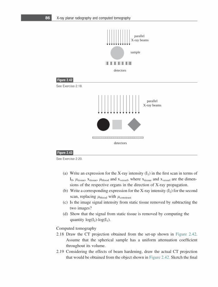
(a) Write an expression for the X-ray intensity (I1) in the first scan in terms ofI0, ltissue, xtissue, lblood and xvessel, where xtissue and xvessel are the dimen-sions of the respective organs in the direction of X-ray propagation.
(b) Write a corresponding expression for the X-ray intensity (I2) for the secondscan, replacing lblood with lconstrast
(c) Is the image signal intensity from static tissue removed by subtracting thetwo images?
(d) Show that the signal from static tissue is removed by computing thequantity log(I2)-log(I1).
Computed tomography2.18 Draw the CT projection obtained from the set-up shown in Figure 2.42.
Assume that the spherical sample has a uniform attenuation coefficientthroughout its volume.
2.19 Considering the effects of beam hardening, draw the actual CT projectionthat would be obtained from the object shown in Figure 2.42. Sketch the final
srotceted
lellarapsmaeb yar-X
Figure 2.43
See Exercise 2.20.
srotceted
elpmas
lellarapsmaeb yar-X
Figure 2.42
See Exercise 2.18.
86 X-ray planar radiography and computed tomography
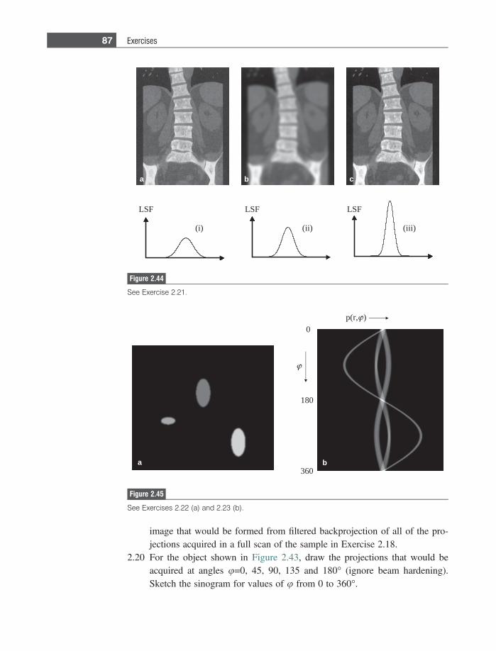
image that would be formed from filtered backprojection of all of the pro-jections acquired in a full scan of the sample in Exercise 2.18.
2.20 For the object shown in Figure 2.43, draw the projections that would beacquired at angles u=0, 45, 90, 135 and 180� (ignore beam hardening).Sketch the sinogram for values of u from 0 to 360�.
LSF
(i) (iii)
LSF LSF
a b c
(ii)
Figure 2.44
See Exercise 2.21.
a
180
0
360
p(r, )
b
Figure 2.45
See Exercises 2.22 (a) and 2.23 (b).
87 Exercises
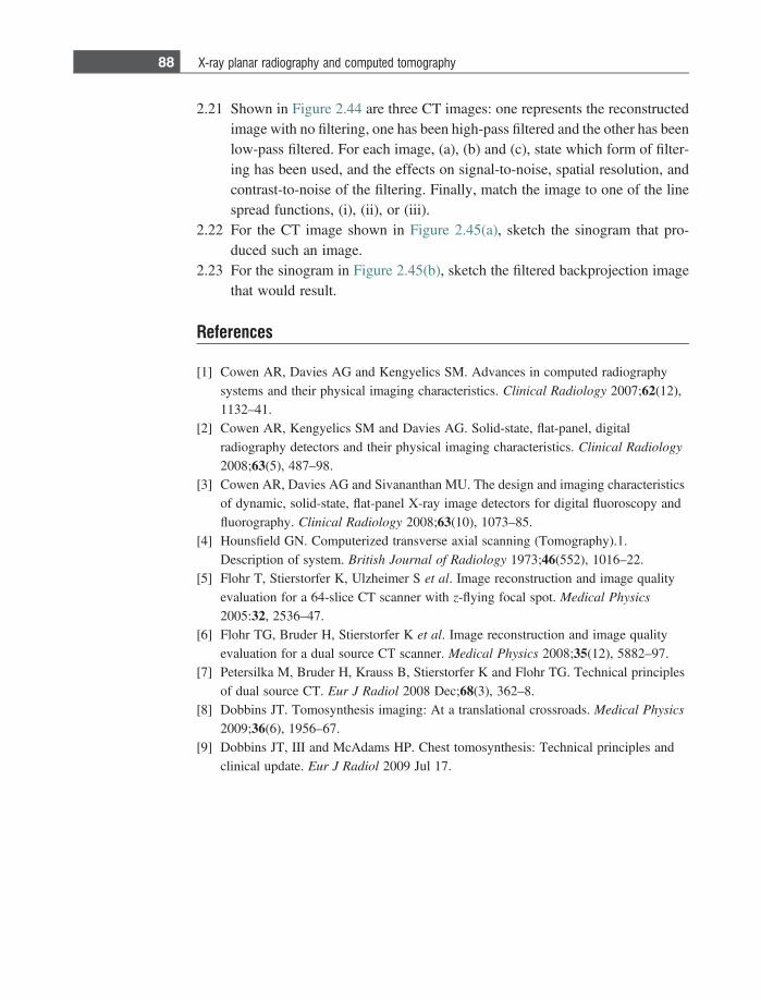
2.21 Shown in Figure 2.44 are three CT images: one represents the reconstructedimage with no filtering, one has been high-pass filtered and the other has beenlow-pass filtered. For each image, (a), (b) and (c), state which form of filter-ing has been used, and the effects on signal-to-noise, spatial resolution, andcontrast-to-noise of the filtering. Finally, match the image to one of the linespread functions, (i), (ii), or (iii).
2.22 For the CT image shown in Figure 2.45(a), sketch the sinogram that pro-duced such an image.
2.23 For the sinogram in Figure 2.45(b), sketch the filtered backprojection imagethat would result.
References
[1] Cowen AR, Davies AG and Kengyelics SM. Advances in computed radiographysystems and their physical imaging characteristics. Clinical Radiology 2007;62(12),1132–41.
[2] Cowen AR, Kengyelics SM and Davies AG. Solid-state, flat-panel, digitalradiography detectors and their physical imaging characteristics. Clinical Radiology
2008;63(5), 487–98.[3] Cowen AR, Davies AG and Sivananthan MU. The design and imaging characteristics
of dynamic, solid-state, flat-panel X-ray image detectors for digital fluoroscopy andfluorography. Clinical Radiology 2008;63(10), 1073–85.
[4] Hounsfield GN. Computerized transverse axial scanning (Tomography).1.Description of system. British Journal of Radiology 1973;46(552), 1016–22.
[5] Flohr T, Stierstorfer K, Ulzheimer S et al. Image reconstruction and image qualityevaluation for a 64-slice CT scanner with z-flying focal spot. Medical Physics
2005:32, 2536–47.[6] Flohr TG, Bruder H, Stierstorfer K et al. Image reconstruction and image quality
evaluation for a dual source CT scanner. Medical Physics 2008;35(12), 5882–97.[7] Petersilka M, Bruder H, Krauss B, Stierstorfer K and Flohr TG. Technical principles
of dual source CT. Eur J Radiol 2008 Dec;68(3), 362–8.[8] Dobbins JT. Tomosynthesis imaging: At a translational crossroads. Medical Physics
2009;36(6), 1956–67.[9] Dobbins JT, III and McAdams HP. Chest tomosynthesis: Technical principles and
clinical update. Eur J Radiol 2009 Jul 17.
88 X-ray planar radiography and computed tomography
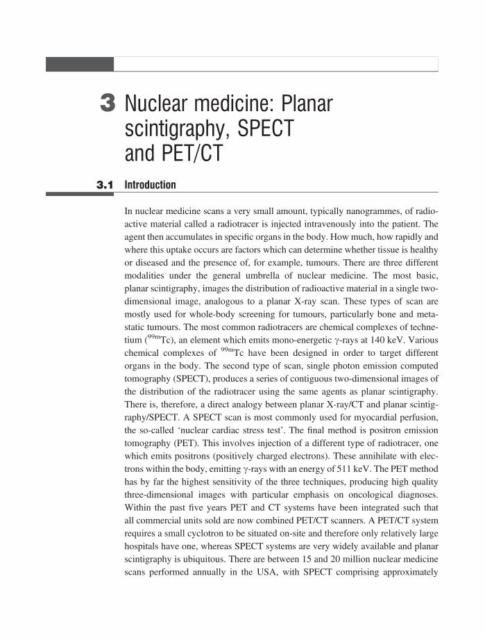
3 Nuclear medicine: Planarscintigraphy, SPECTand PET/CT
3.1 Introduction
In nuclear medicine scans a very small amount, typically nanogrammes, of radio-active material called a radiotracer is injected intravenously into the patient. Theagent then accumulates in specific organs in the body. How much, how rapidly andwhere this uptake occurs are factors which can determine whether tissue is healthyor diseased and the presence of, for example, tumours. There are three differentmodalities under the general umbrella of nuclear medicine. The most basic,planar scintigraphy, images the distribution of radioactive material in a single two-dimensional image, analogous to a planar X-ray scan. These types of scan aremostly used for whole-body screening for tumours, particularly bone and meta-static tumours. The most common radiotracers are chemical complexes of techne-tium (99mTc), an element which emits mono-energetic c-rays at 140 keV. Variouschemical complexes of 99mTc have been designed in order to target differentorgans in the body. The second type of scan, single photon emission computedtomography (SPECT), produces a series of contiguous two-dimensional images ofthe distribution of the radiotracer using the same agents as planar scintigraphy.There is, therefore, a direct analogy between planar X-ray/CT and planar scintig-raphy/SPECT. A SPECT scan is most commonly used for myocardial perfusion,the so-called ‘nuclear cardiac stress test’. The final method is positron emissiontomography (PET). This involves injection of a different type of radiotracer, onewhich emits positrons (positively charged electrons). These annihilate with elec-trons within the body, emitting c-rays with an energy of 511 keV. The PET methodhas by far the highest sensitivity of the three techniques, producing high qualitythree-dimensional images with particular emphasis on oncological diagnoses.Within the past five years PET and CT systems have been integrated such thatall commercial units sold are now combined PET/CT scanners. A PET/CT systemrequires a small cyclotron to be situated on-site and therefore only relatively largehospitals have one, whereas SPECT systems are very widely available and planarscintigraphy is ubiquitous. There are between 15 and 20 million nuclear medicinescans performed annually in the USA, with SPECT comprising approximately
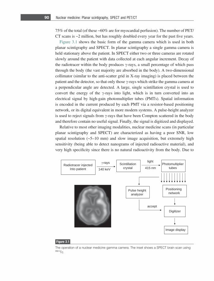
75% of the total (of these ~60% are for myocardial perfusion). The number of PET/CT scans is ~2 million, but has roughly doubled every year for the past five years.
Figure 3.1 shows the basic form of the gamma camera which is used in bothplanar scintigraphy and SPECT. In planar scintigraphy a single gamma camera isheld stationary above the patient. In SPECT either two or three cameras are rotatedslowly around the patient with data collected at each angular increment. Decay ofthe radiotracer within the body produces c-rays, a small percentage of which passthrough the body (the vast majority are absorbed in the body). A two-dimensionalcollimator (similar to the anti-scatter grid in X-ray imaging) is placed between thepatient and the detector, so that only those c-rays which strike the gamma camera ata perpendicular angle are detected. A large, single scintillation crystal is used toconvert the energy of the c-rays into light, which is in turn converted into anelectrical signal by high-gain photomultiplier tubes (PMTs). Spatial informationis encoded in the current produced by each PMT via a resistor-based positioningnetwork, or its digital equivalent in more modern systems. A pulse-height analyzeris used to reject signals from c-rays that have been Compton scattered in the bodyand therefore contain no useful signal. Finally, the signal is digitized and displayed.
Relative to most other imaging modalities, nuclear medicine scans (in particularplanar scintigraphy and SPECT) are characterized as having a poor SNR, lowspatial resolution (~5–10 mm) and slow image acquisition, but extremely highsensitivity (being able to detect nanograms of injected radioactive material), andvery high specificity since there is no natural radioactivity from the body. Due to
detcejni recartoidaRtneitap otnI Vek 041
noitallitnicSlatsyrc
thgil
mn 514reilpitlumotohP
sebut
gninoitisoPkrowten
thgieh esluPrezylana
tpeccarezitigiD
yalpsid egamI
syar-
Figure 3.1
The operation of a nuclear medicine gamma camera. The inset shows a SPECT brain scan using99mTc.
90 Nuclear medicine: Planar scintigraphy, SPECT and PET/CT
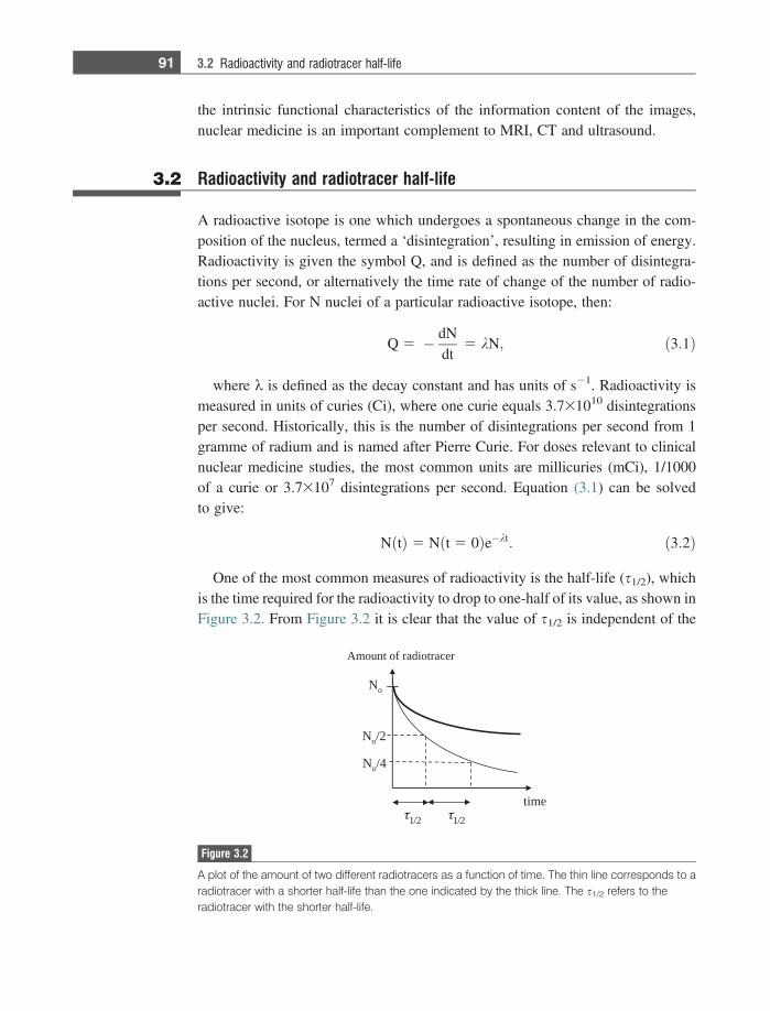
the intrinsic functional characteristics of the information content of the images,nuclear medicine is an important complement to MRI, CT and ultrasound.
3.2 Radioactivity and radiotracer half-life
A radioactive isotope is one which undergoes a spontaneous change in the com-position of the nucleus, termed a ‘disintegration’, resulting in emission of energy.Radioactivity is given the symbol Q, and is defined as the number of disintegra-tions per second, or alternatively the time rate of change of the number of radio-active nuclei. For N nuclei of a particular radioactive isotope, then:
Q 5 � dNdt
5 kN; ð3:1Þ
where k is defined as the decay constant and has units of s21. Radioactivity ismeasured in units of curies (Ci), where one curie equals 3.731010 disintegrationsper second. Historically, this is the number of disintegrations per second from 1gramme of radium and is named after Pierre Curie. For doses relevant to clinicalnuclear medicine studies, the most common units are millicuries (mCi), 1/1000of a curie or 3.73107 disintegrations per second. Equation (3.1) can be solvedto give:
NðtÞ 5 N t 5 0ð Þe�kt: ð3:2Þ
One of the most common measures of radioactivity is the half-life (s1/2), whichis the time required for the radioactivity to drop to one-half of its value, as shown inFigure 3.2. From Figure 3.2 it is clear that the value of s1/2 is independent of the
No
emit
2/1
No 2/
No 4/
recartoidar fo tnuomA
2/1
Figure 3.2
A plot of the amount of two different radiotracers as a function of time. The thin line corresponds to aradiotracer with a shorter half-life than the one indicated by the thick line. The s1/2 refers to theradiotracer with the shorter half-life.
91 3.2 Radioactivity and radiotracer half-life

value of N. Since the value of k is also independent of N, s1/2 also corresponds tothe time for the number of radioactive nuclei to drop by half, and so from Equation(3.2) the value of s1/2 is given by:
s1=2 5ln 2k: ð3:3Þ
In nuclear medicine scans the total radioactive dose experienced by the patient islimited by federal safely guidelines. To calculate the dose, the biological half-lifeof the radiotracer (how long the radiotracer remains in the body) must also beconsidered. In many cases, excretion of the radiotracer from tissue is an exponen-tial decay which can be characterized by a corresponding biological half-life,s1/2,bio. The effective half-life (s1/2,eff) of the radioactivity within the body is acombination of the two half-lives and is given by:
s1=2;eff 5s1=2s1=2;bio
s1=2 1 s1=2;bio: ð3:4Þ
Therefore, the value of s1/2,eff is always less than the shorter of the two half-lives, s1/2 and s1/2,bio.
Example 3.1 Two patients undergo nuclear medicine scans. One receives a dose of radiotracer Aand the other radioatracer B. The half-life of A is 6 hours and of B is 24 hours. Ifthe administered dose of radiotracer A is three times that of radiotracer B, and thebiological half-lives of A and B are 6 and 12 hours respectively, at what time is theradioactivity in the body the same for the two patients?
Solution Mathematically we can solve the following for the time t:
3e�tkA 5 e�tkB :
The values of kA and kB can be derived from Equation (3.4) and are 6.42 3 1025
and 2.41 3 1025 s21, respectively. Solving for t gives a value of 7.63 hours.
3.3 Properties of radiotracers for nuclear medicine
The ideal properties of a radiotracer for planar scintigraphy and SPECT include:
(i) A radioactive half-life that is short enough to produce significant radioactivitywithout requiring a very large initial dose, but not so short that there issignificant decay before the required post-injection delay to allow the radio-tracer to clear the blood and distribute in the relevant organs.
92 Nuclear medicine: Planar scintigraphy, SPECT and PET/CT
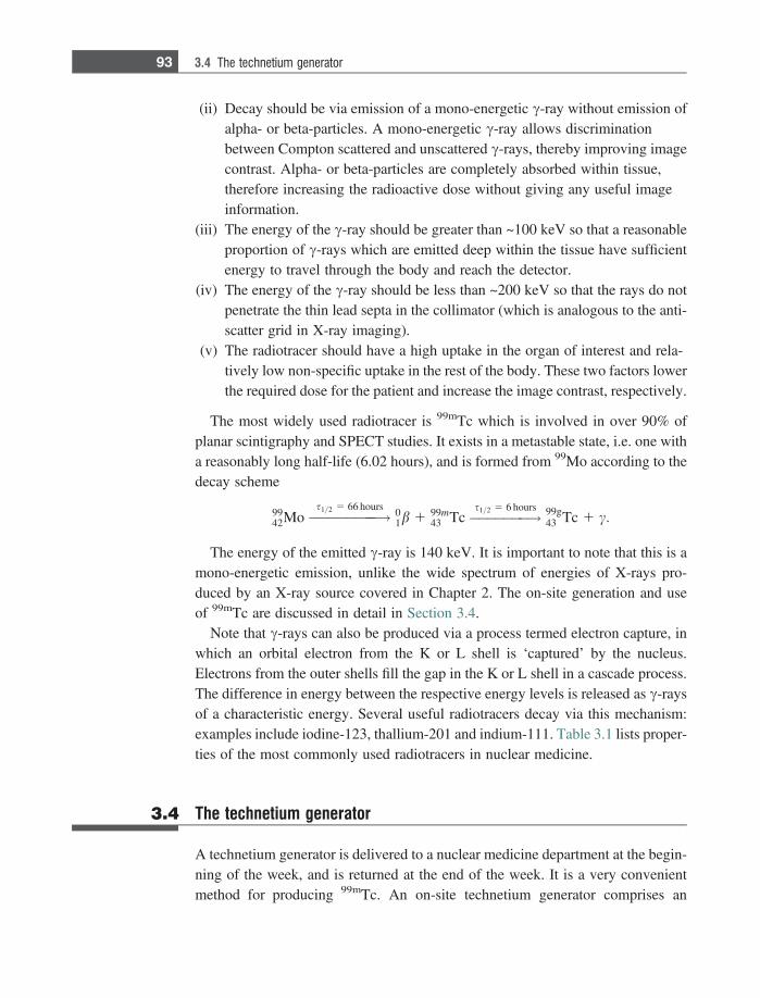
(ii) Decay should be via emission of a mono-energetic c-ray without emission ofalpha- or beta-particles. A mono-energetic c-ray allows discriminationbetween Compton scattered and unscattered c-rays, thereby improving imagecontrast. Alpha- or beta-particles are completely absorbed within tissue,therefore increasing the radioactive dose without giving any useful imageinformation.
(iii) The energy of the c-ray should be greater than ~100 keV so that a reasonableproportion of c-rays which are emitted deep within the tissue have sufficientenergy to travel through the body and reach the detector.
(iv) The energy of the c-ray should be less than ~200 keV so that the rays do notpenetrate the thin lead septa in the collimator (which is analogous to the anti-scatter grid in X-ray imaging).
(v) The radiotracer should have a high uptake in the organ of interest and rela-tively low non-specific uptake in the rest of the body. These two factors lowerthe required dose for the patient and increase the image contrast, respectively.
The most widely used radiotracer is 99mTc which is involved in over 90% ofplanar scintigraphy and SPECT studies. It exists in a metastable state, i.e. one witha reasonably long half-life (6.02 hours), and is formed from 99Mo according to thedecay scheme
9942Mo !s1=2 5 66 hours
01b 1 99m
43 Tc !s1=2 5 6 hours 99g43 Tc 1 c:
The energy of the emitted c-ray is 140 keV. It is important to note that this is amono-energetic emission, unlike the wide spectrum of energies of X-rays pro-duced by an X-ray source covered in Chapter 2. The on-site generation and useof 99mTc are discussed in detail in Section 3.4.
Note that c-rays can also be produced via a process termed electron capture, inwhich an orbital electron from the K or L shell is ‘captured’ by the nucleus.Electrons from the outer shells fill the gap in the K or L shell in a cascade process.The difference in energy between the respective energy levels is released as c-raysof a characteristic energy. Several useful radiotracers decay via this mechanism:examples include iodine-123, thallium-201 and indium-111. Table 3.1 lists proper-ties of the most commonly used radiotracers in nuclear medicine.
3.4 The technetium generator
A technetium generator is delivered to a nuclear medicine department at the begin-ning of the week, and is returned at the end of the week. It is a very convenientmethod for producing 99mTc. An on-site technetium generator comprises an
93 3.4 The technetium generator
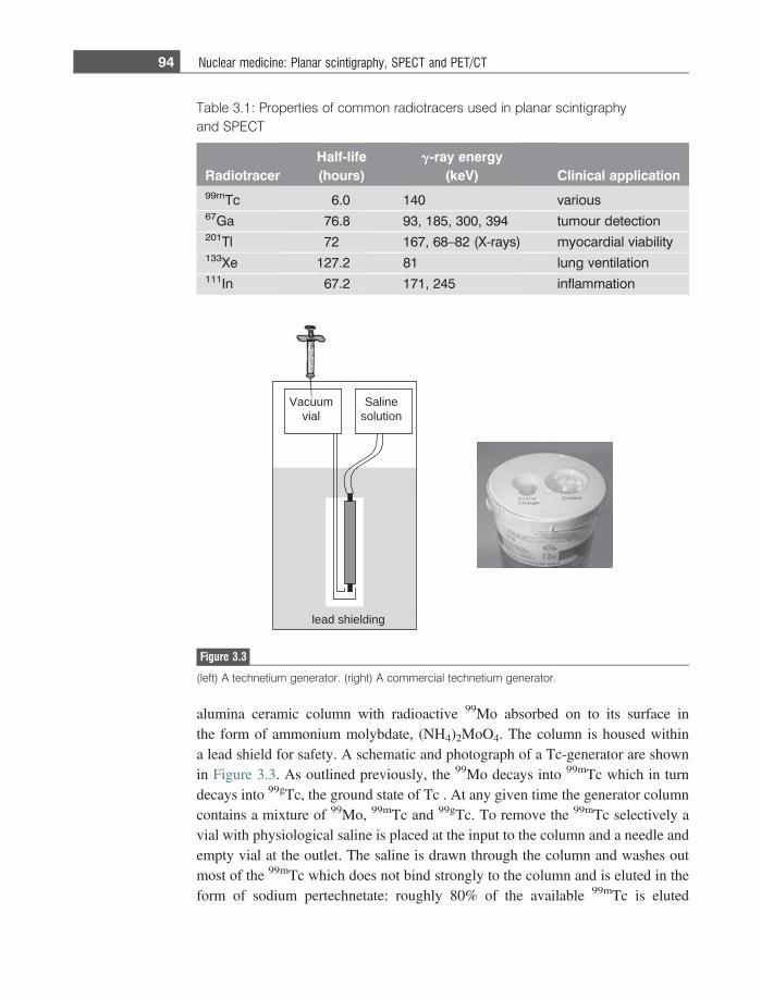
alumina ceramic column with radioactive 99Mo absorbed on to its surface inthe form of ammonium molybdate, (NH4)2MoO4. The column is housed withina lead shield for safety. A schematic and photograph of a Tc-generator are shownin Figure 3.3. As outlined previously, the 99Mo decays into 99mTc which in turndecays into 99gTc, the ground state of Tc . At any given time the generator columncontains a mixture of 99Mo, 99mTc and 99gTc. To remove the 99mTc selectively avial with physiological saline is placed at the input to the column and a needle andempty vial at the outlet. The saline is drawn through the column and washes outmost of the 99mTc which does not bind strongly to the column and is eluted in theform of sodium pertechnetate: roughly 80% of the available 99mTc is eluted
Salinesolution
Vacuumvial
lead shielding
Figure 3.3
(left) A technetium generator. (right) A commercial technetium generator.
Table 3.1: Properties of common radiotracers used in planar scintigraphyand SPECT
RadiotracerHalf-life(hours)
g-ray energy(keV) Clinical application
99mTc 6.0 140 various67Ga 76.8 93, 185, 300, 394 tumour detection201Tl 72 167, 68–82 (X-rays) myocardial viability133Xe 127.2 81 lung ventilation111In 67.2 171, 245 inflammation
94 Nuclear medicine: Planar scintigraphy, SPECT and PET/CT

compared to less than 1% of the 99Mo. Appropriate radioassays are then carried outto determine the concentration and purity of the eluted 99mTc, with Al and 99Moimpurities required to be below certain safety levels. Typically, the technetium iseluted every 24 hours, and the generator is replaced once a week. Most nuclearmedicine scans are therefore scheduled for the beginning of a week.
The time-dependence of the radioactivity can be analyzed as a two-step process.The number of 99Mo atoms, denoted by N1, decreases with time from an initialmaximum value N0 at time t = 0. This radioactive decay produces N2 atoms of99mTc, which decay to form N3 atoms of 99gTc, the final stable product:
99Mo !k1 99mTc !k2 99gTc
N1ð Þ N2ð Þ N3ð Þ:
The values of k1 and k2, derived from the respective half-lives, are 2.9231026
s21 and 3.2131025 s21, respectively. The decay of the 99Mo (termed the parentnucleus) is given by Equation (3.2), N1 5 Noe�k1t. Since there is a two-step decayprocess, the amount of 99mTc increases due to the decay of 99Mo, but decreases dueto its own decay to 99gTc:
dN2
dt5 k1N1�k2N20
dN2
dt1 k2N2 5 k1N1: ð3:5Þ
There are a number of methods for solving this simple first order differentialequation. For example, the homogeneous and particular equations can be solved:
homogeneousð ÞN2 5 Ce�k2t
ðparticularÞN2 5 De�k1t: ð3:6Þ
For the particular solution, solving for D gives:
D 5k1N0
k2 � k1: ð3:7Þ
Adding together the homogeneous and particular solutions:
N2 5 Ce�k2t 1k1N0
k2 � k1e�k1t: ð3:8Þ
Since we know that N2 = 0 at t = 0, using this boundary condition we can solvefor the constant C:
C 5 � k1N0
k2 � k1: ð3:9Þ
95 3.4 The technetium generator
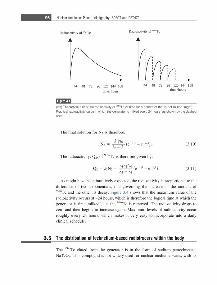
The final solution for N2 is therefore:
N2 5k1N0
k2 � k1e�k1t � e�k2t� �
: ð3:10Þ
The radioactivity, Q2, of 99mTc is therefore given by:
Q2 5 k2N2 5k1k2N0
k2 � k1e�k1t � e�k2t� �
: ð3:11Þ
As might have been intuitively expected, the radioactivity is proportional to thedifference of two exponentials, one governing the increase in the amount of99mTc and the other its decay. Figure 3.4 shows that the maximum value of theradioactivity occurs at ~24 hours, which is therefore the logical time at which thegenerator is first ‘milked’, i.e. the 99mTc is removed. The radioactivity drops tozero and then begins to increase again. Maximum levels of radioactivity occurroughly every 24 hours, which makes it very easy to incorporate into a dailyclinical schedule.
3.5 The distribution of technetium-based radiotracers within the body
The 99mTc eluted from the generator is in the form of sodium pertechnetate,NaTcO4. This compound is not widely used for nuclear medicine scans, with its
42 0216984 86144127
tcaoidaR tivi foy m99 cT
t sruoh/emit sruoh/emi
42 0216984 86144127
tcaoidaR tivi foy m99 cT
Figure 3.4
(left) Theoretical plot of the radioactivity of 99mTc vs time for a generator that is not milked. (right)Practical radioactivity curve in which the generator is milked every 24 hours, as shown by the dashedlines.
96 Nuclear medicine: Planar scintigraphy, SPECT and PET/CT
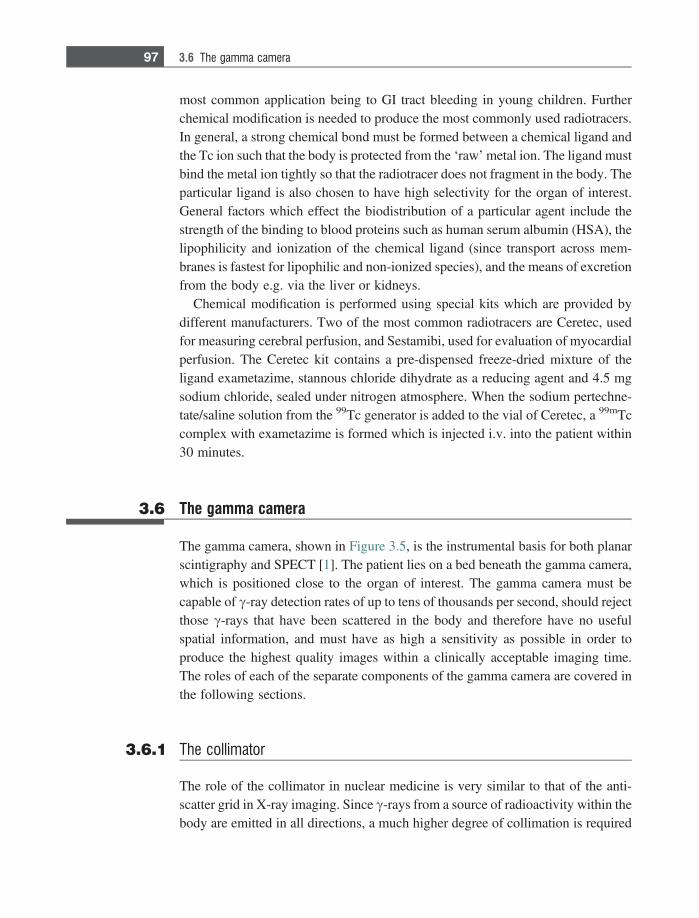
most common application being to GI tract bleeding in young children. Furtherchemical modification is needed to produce the most commonly used radiotracers.In general, a strong chemical bond must be formed between a chemical ligand andthe Tc ion such that the body is protected from the ‘raw’ metal ion. The ligand mustbind the metal ion tightly so that the radiotracer does not fragment in the body. Theparticular ligand is also chosen to have high selectivity for the organ of interest.General factors which effect the biodistribution of a particular agent include thestrength of the binding to blood proteins such as human serum albumin (HSA), thelipophilicity and ionization of the chemical ligand (since transport across mem-branes is fastest for lipophilic and non-ionized species), and the means of excretionfrom the body e.g. via the liver or kidneys.
Chemical modification is performed using special kits which are provided bydifferent manufacturers. Two of the most common radiotracers are Ceretec, usedfor measuring cerebral perfusion, and Sestamibi, used for evaluation of myocardialperfusion. The Ceretec kit contains a pre-dispensed freeze-dried mixture of theligand exametazime, stannous chloride dihydrate as a reducing agent and 4.5 mgsodium chloride, sealed under nitrogen atmosphere. When the sodium pertechne-tate/saline solution from the 99Tc generator is added to the vial of Ceretec, a 99mTccomplex with exametazime is formed which is injected i.v. into the patient within30 minutes.
3.6 The gamma camera
The gamma camera, shown in Figure 3.5, is the instrumental basis for both planarscintigraphy and SPECT [1]. The patient lies on a bed beneath the gamma camera,which is positioned close to the organ of interest. The gamma camera must becapable of c-ray detection rates of up to tens of thousands per second, should rejectthose c-rays that have been scattered in the body and therefore have no usefulspatial information, and must have as high a sensitivity as possible in order toproduce the highest quality images within a clinically acceptable imaging time.The roles of each of the separate components of the gamma camera are covered inthe following sections.
3.6.1 The collimator
The role of the collimator in nuclear medicine is very similar to that of the anti-scatter grid in X-ray imaging. Since c-rays from a source of radioactivity within thebody are emitted in all directions, a much higher degree of collimation is required
97 3.6 The gamma camera
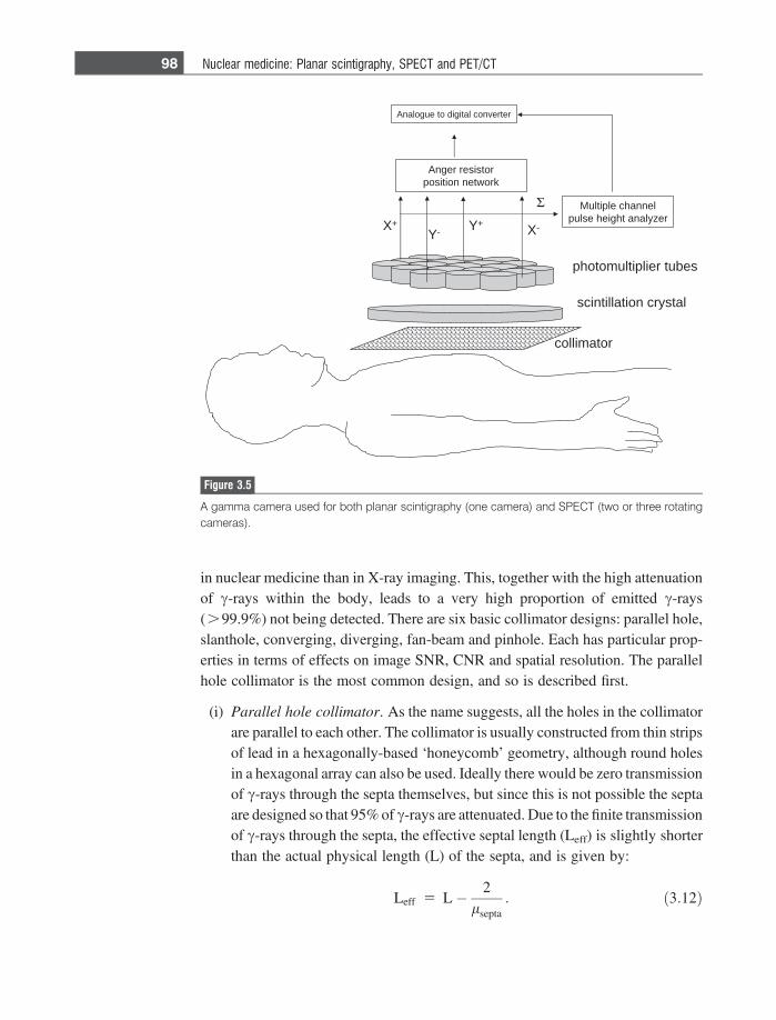
in nuclear medicine than in X-ray imaging. This, together with the high attenuationof c-rays within the body, leads to a very high proportion of emitted c-rays(.99.9%) not being detected. There are six basic collimator designs: parallel hole,slanthole, converging, diverging, fan-beam and pinhole. Each has particular prop-erties in terms of effects on image SNR, CNR and spatial resolution. The parallelhole collimator is the most common design, and so is described first.
(i) Parallel hole collimator. As the name suggests, all the holes in the collimatorare parallel to each other. The collimator is usually constructed from thin stripsof lead in a hexagonally-based ‘honeycomb’ geometry, although round holesin a hexagonal array can also be used. Ideally there would be zero transmissionof c-rays through the septa themselves, but since this is not possible the septaare designed so that 95% of c-rays are attenuated. Due to the finite transmissionof c-rays through the septa, the effective septal length (Leff) is slightly shorterthan the actual physical length (L) of the septa, and is given by:
Leff 5 L� 2lsepta
: ð3:12Þ
X+
Y-Y+
X-
Σ Multiple channel
pulse height analyzer
Anger resistor
position network
Analogue to digital converter
collimator
scintillation crystal
photomultiplier tubes
Figure 3.5
A gamma camera used for both planar scintigraphy (one camera) and SPECT (two or three rotatingcameras).
98 Nuclear medicine: Planar scintigraphy, SPECT and PET/CT
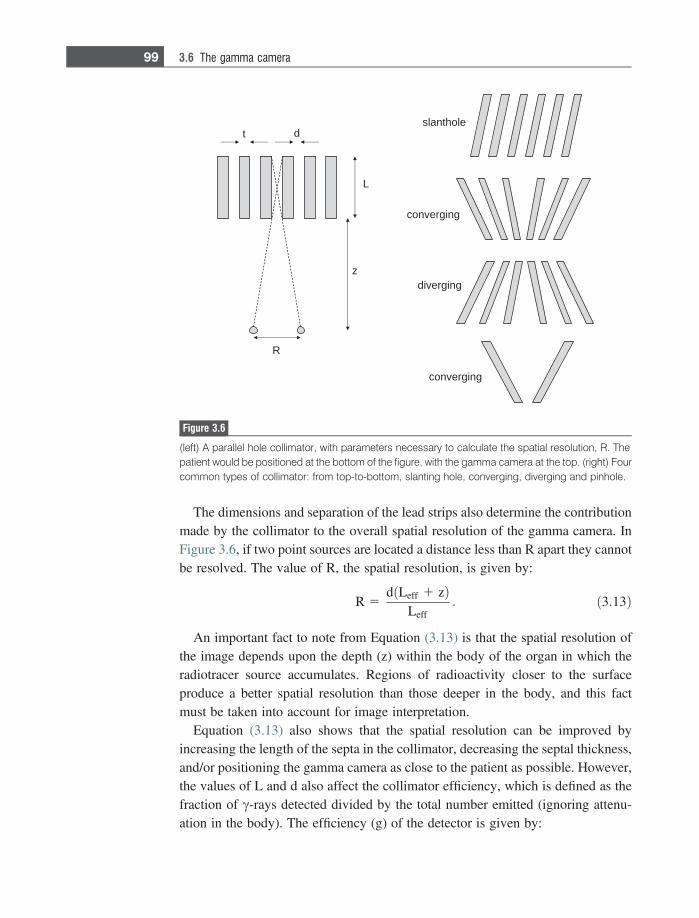
The dimensions and separation of the lead strips also determine the contributionmade by the collimator to the overall spatial resolution of the gamma camera. InFigure 3.6, if two point sources are located a distance less than R apart they cannotbe resolved. The value of R, the spatial resolution, is given by:
R 5d Leff 1 zð Þ
Leff: ð3:13Þ
An important fact to note from Equation (3.13) is that the spatial resolution ofthe image depends upon the depth (z) within the body of the organ in which theradiotracer source accumulates. Regions of radioactivity closer to the surfaceproduce a better spatial resolution than those deeper in the body, and this factmust be taken into account for image interpretation.
Equation (3.13) also shows that the spatial resolution can be improved byincreasing the length of the septa in the collimator, decreasing the septal thickness,and/or positioning the gamma camera as close to the patient as possible. However,the values of L and d also affect the collimator efficiency, which is defined as thefraction of c-rays detected divided by the total number emitted (ignoring attenu-ation in the body). The efficiency (g) of the detector is given by:
L
slanthole
converging
converging
diverging
dt
R
z
Figure 3.6
(left) A parallel hole collimator, with parameters necessary to calculate the spatial resolution, R. Thepatient would be positioned at the bottom of the figure, with the gamma camera at the top. (right) Fourcommon types of collimator: from top-to-bottom, slanting hole, converging, diverging and pinhole.
99 3.6 The gamma camera
g � K2 d2
L2eff
d2
d 1 tð Þ2; ð3:14Þ
where the value of K depends upon the particular hole-geometry and has a valueof 0.26 for hexagonal holes in a hexagonal array. It is clear from Equation (3.14) thatthere is an intrinsic trade-off between spatial resolution and collimator efficiency.
Collimators used for 99mTc imaging are referred to as low-energy (140 keVc-rays): those with relatively large holes are termed low-energy all-purpose(LEAP) and those with smaller holes and longer septa are called low-energyhigh-resolution (LEHR). Medium energy and high energy collimators have septaof increasing thickness and are used for 67Ga/111In and 131I, respectively.
(ii) Slanthole collimators consist of parallel septa which are all tilted at the sameangle with respect to the detection crystal. They are used primarily for breastand cardiac imaging.
(iii) Converging collimators have the holes focused towards the body, with thecentre of curvature ideally located at the middle of the imaging field-of-view(FOV). A converging collimator is used to magnify the image and increasethe spatial resolution.
(iv) A diverging collimator is essentially a converging collimator that has beenturned around. This enables a larger FOV, compared to a parallel hole col-limator, to be imaged. One application is planar scintigraphy of the wholebody.
(v) Fan-beam collimators are used primarily for brain and heart studies. The twodimensions of the collimator have different geometries: in the head/footdirection the holes are parallel, whereas in the radial direction they are similarto a converging collimator. Thus, these types of collimator provide imagemagnification over a reduced FOV.
(vi) Pinhole collimators are used for imaging very small organs such as the thyroidand parathyroid. These collimators have a single hole with interchangeableinserts that come with a 3, 4 or 6 mm aperture. A pinhole collimator producesan image with significant magnification and higher spatial resolution, but alsoproduces geometric distortion, particularly at the edges of the image.
3.6.2 The detector scintillation crystal and coupled photomultiplier tubes
c-rays not attenuated in the body are detected using a scintillation crystal whichconverts their energy into light. In the gamma camera, the detector is a large singlecrystal of thallium-activated sodium iodide, NaI(Tl), approximately 40–50 cm
100 Nuclear medicine: Planar scintigraphy, SPECT and PET/CT
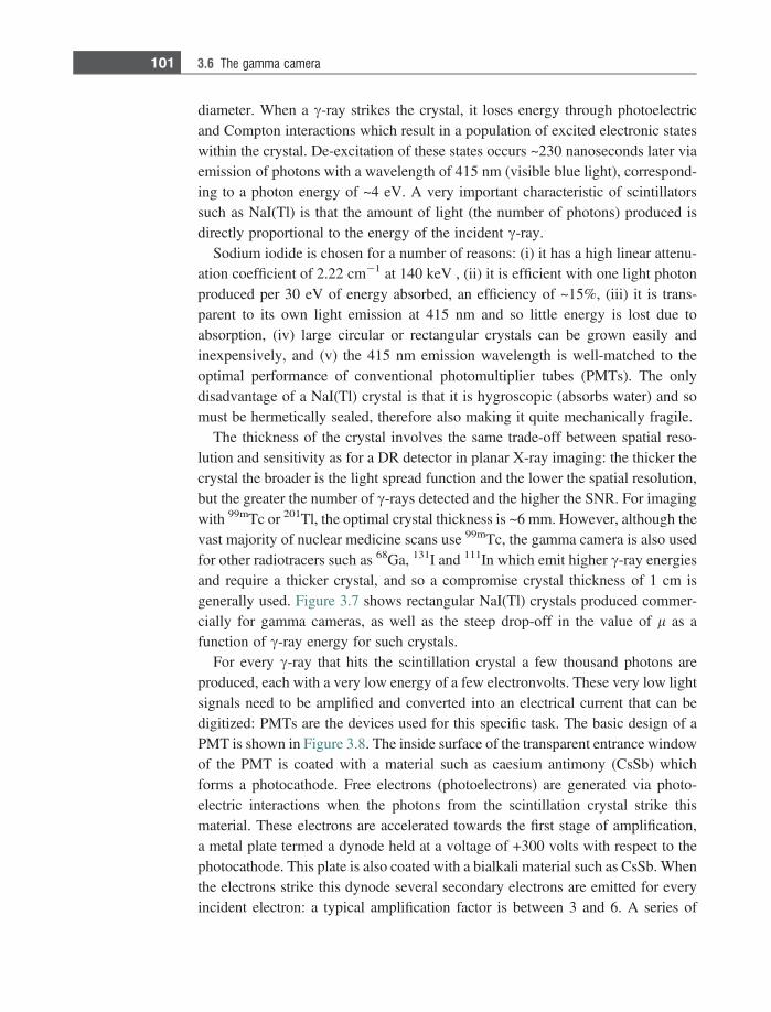
diameter. When a c-ray strikes the crystal, it loses energy through photoelectricand Compton interactions which result in a population of excited electronic stateswithin the crystal. De-excitation of these states occurs ~230 nanoseconds later viaemission of photons with a wavelength of 415 nm (visible blue light), correspond-ing to a photon energy of ~4 eV. A very important characteristic of scintillatorssuch as NaI(Tl) is that the amount of light (the number of photons) produced isdirectly proportional to the energy of the incident c-ray.
Sodium iodide is chosen for a number of reasons: (i) it has a high linear attenu-ation coefficient of 2.22 cm21 at 140 keV , (ii) it is efficient with one light photonproduced per 30 eV of energy absorbed, an efficiency of ~15%, (iii) it is trans-parent to its own light emission at 415 nm and so little energy is lost due toabsorption, (iv) large circular or rectangular crystals can be grown easily andinexpensively, and (v) the 415 nm emission wavelength is well-matched to theoptimal performance of conventional photomultiplier tubes (PMTs). The onlydisadvantage of a NaI(Tl) crystal is that it is hygroscopic (absorbs water) and somust be hermetically sealed, therefore also making it quite mechanically fragile.
The thickness of the crystal involves the same trade-off between spatial reso-lution and sensitivity as for a DR detector in planar X-ray imaging: the thicker thecrystal the broader is the light spread function and the lower the spatial resolution,but the greater the number of c-rays detected and the higher the SNR. For imagingwith 99mTc or 201Tl, the optimal crystal thickness is ~6 mm. However, although thevast majority of nuclear medicine scans use 99mTc, the gamma camera is also usedfor other radiotracers such as 68Ga, 131I and 111In which emit higher c-ray energiesand require a thicker crystal, and so a compromise crystal thickness of 1 cm isgenerally used. Figure 3.7 shows rectangular NaI(Tl) crystals produced commer-cially for gamma cameras, as well as the steep drop-off in the value of l as afunction of c-ray energy for such crystals.
For every c-ray that hits the scintillation crystal a few thousand photons areproduced, each with a very low energy of a few electronvolts. These very low lightsignals need to be amplified and converted into an electrical current that can bedigitized: PMTs are the devices used for this specific task. The basic design of aPMT is shown in Figure 3.8. The inside surface of the transparent entrance windowof the PMT is coated with a material such as caesium antimony (CsSb) whichforms a photocathode. Free electrons (photoelectrons) are generated via photo-electric interactions when the photons from the scintillation crystal strike thismaterial. These electrons are accelerated towards the first stage of amplification,a metal plate termed a dynode held at a voltage of +300 volts with respect to thephotocathode. This plate is also coated with a bialkali material such as CsSb. Whenthe electrons strike this dynode several secondary electrons are emitted for everyincident electron: a typical amplification factor is between 3 and 6. A series of
101 3.6 The gamma camera
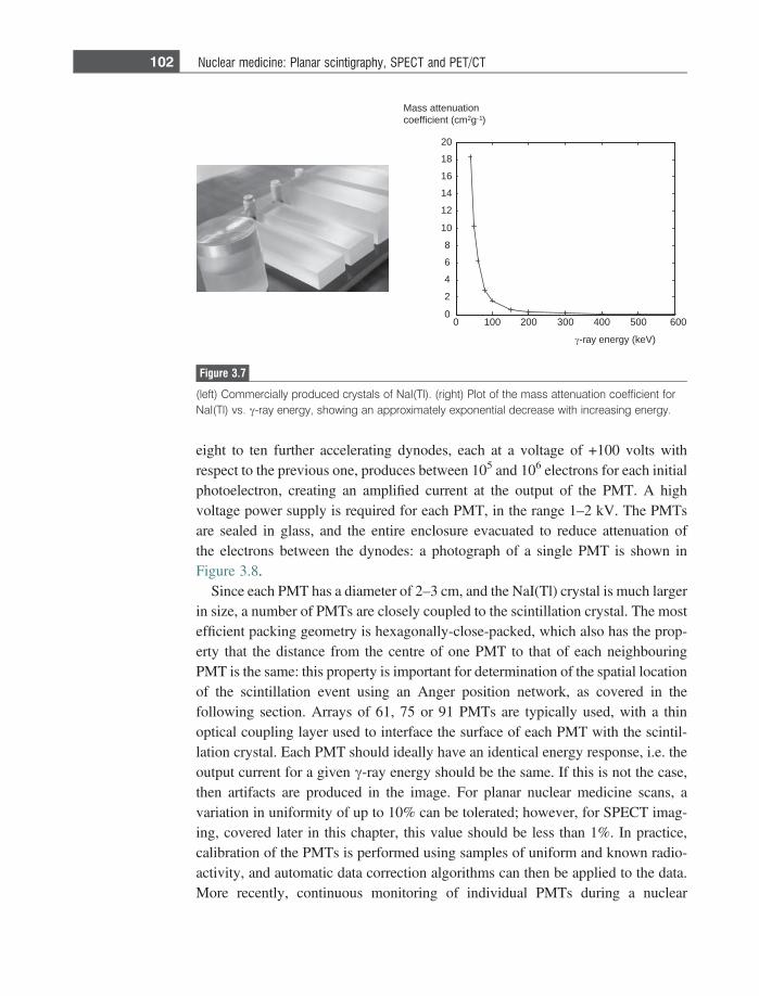
eight to ten further accelerating dynodes, each at a voltage of +100 volts withrespect to the previous one, produces between 105 and 106 electrons for each initialphotoelectron, creating an amplified current at the output of the PMT. A highvoltage power supply is required for each PMT, in the range 1–2 kV. The PMTsare sealed in glass, and the entire enclosure evacuated to reduce attenuation ofthe electrons between the dynodes: a photograph of a single PMT is shown inFigure 3.8.
Since each PMT has a diameter of 2–3 cm, and the NaI(Tl) crystal is much largerin size, a number of PMTs are closely coupled to the scintillation crystal. The mostefficient packing geometry is hexagonally-close-packed, which also has the prop-erty that the distance from the centre of one PMT to that of each neighbouringPMT is the same: this property is important for determination of the spatial locationof the scintillation event using an Anger position network, as covered in thefollowing section. Arrays of 61, 75 or 91 PMTs are typically used, with a thinoptical coupling layer used to interface the surface of each PMT with the scintil-lation crystal. Each PMT should ideally have an identical energy response, i.e. theoutput current for a given c-ray energy should be the same. If this is not the case,then artifacts are produced in the image. For planar nuclear medicine scans, avariation in uniformity of up to 10% can be tolerated; however, for SPECT imag-ing, covered later in this chapter, this value should be less than 1%. In practice,calibration of the PMTs is performed using samples of uniform and known radio-activity, and automatic data correction algorithms can then be applied to the data.More recently, continuous monitoring of individual PMTs during a nuclear
0 100 200 300 400 500 6000
2
4
6
8
10
12
14
16
18
20
-ray energy (keV)
Mass attenuation coefficient (cm2g-1)
Figure 3.7
(left) Commercially produced crystals of NaI(Tl). (right) Plot of the mass attenuation coefficient forNaI(Tl) vs. c-ray energy, showing an approximately exponential decrease with increasing energy.
102 Nuclear medicine: Planar scintigraphy, SPECT and PET/CT
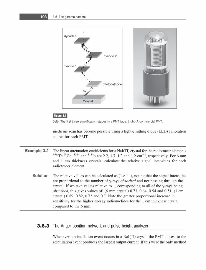
medicine scan has become possible using a light-emitting diode (LED) calibrationsource for each PMT.
Example 3.2 The linear attenuation coefficients for a NaI(Tl) crystal for the radiotracer elements99mTc,68Ga, 131I and 111In are 2.2, 1.7, 1.3 and 1.2 cm21, respectively. For 6 mmand 1 cm thickness crystals, calculate the relative signal intensities for eachradiotracer element.
Solution The relative values can be calculated as (1-e2lx), noting that the signal intensitiesare proportional to the number of c-rays absorbed and not passing through thecrystal. If we take values relative to 1, corresponding to all of the c-rays beingabsorbed, this gives values of: (6 mm crystal) 0.73, 0.64, 0.54 and 0.51, (1 cmcrystal) 0.89, 0.82, 0.73 and 0.7. Note the greater proportional increase insensitivity for the higher energy radionuclides for the 1 cm thickness crystalcompared to the 6 mm.
3.6.3 The Anger position network and pulse height analyzer
Whenever a scintillation event occurs in a NaI(Tl) crystal the PMT closest to thescintillation event produces the largest output current. If this were the only method
hv
photocathode
dynode 1
dynode 2
dynode 3
Crystal
Figure 3.8
(left). The first three amplification stages in a PMT tube. (right) A commercial PMT.
103 3.6 The gamma camera
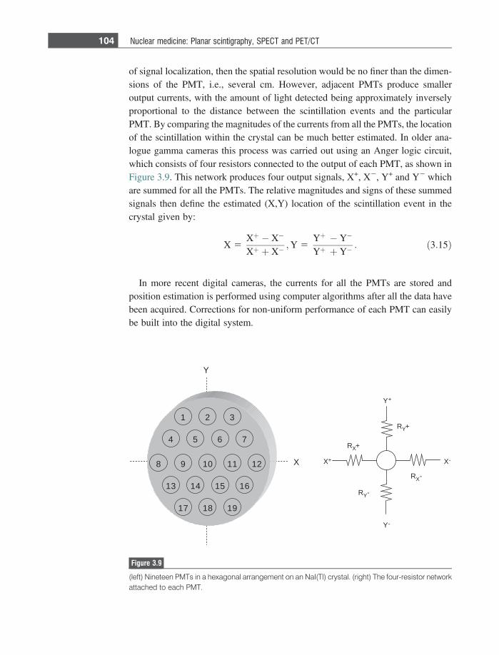
of signal localization, then the spatial resolution would be no finer than the dimen-sions of the PMT, i.e., several cm. However, adjacent PMTs produce smalleroutput currents, with the amount of light detected being approximately inverselyproportional to the distance between the scintillation events and the particularPMT. By comparing the magnitudes of the currents from all the PMTs, the locationof the scintillation within the crystal can be much better estimated. In older ana-logue gamma cameras this process was carried out using an Anger logic circuit,which consists of four resistors connected to the output of each PMT, as shown inFigure 3.9. This network produces four output signals, X+, X2, Y+ and Y2 whichare summed for all the PMTs. The relative magnitudes and signs of these summedsignals then define the estimated (X,Y) location of the scintillation event in thecrystal given by:
X 5Xþ � X�
Xþ þ X�;Y 5
Yþ � Y�
Yþ þ Y�: ð3:15Þ
In more recent digital cameras, the currents for all the PMTs are stored andposition estimation is performed using computer algorithms after all the data havebeen acquired. Corrections for non-uniform performance of each PMT can easilybe built into the digital system.
321
7654
198 10 11 2
1 13 14 15 6
1 17 18 9
Y+
RY+
Y-
X-X+
RX+
RX-
RY-
X
Y
Figure 3.9
(left) Nineteen PMTs in a hexagonal arrangement on an NaI(Tl) crystal. (right) The four-resistor networkattached to each PMT.
104 Nuclear medicine: Planar scintigraphy, SPECT and PET/CT
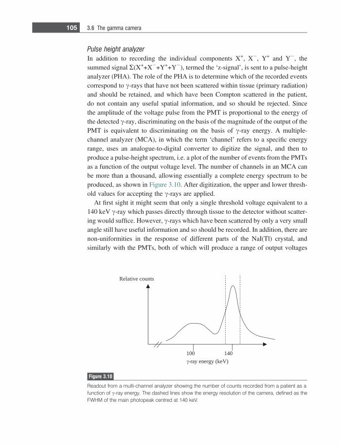
Pulse height analyzer
In addition to recording the individual components X+, X2, Y+ and Y2, thesummed signal R(X++X2+Y++Y2), termed the ‘z-signal’, is sent to a pulse-heightanalyzer (PHA). The role of the PHA is to determine which of the recorded eventscorrespond to c-rays that have not been scattered within tissue (primary radiation)and should be retained, and which have been Compton scattered in the patient,do not contain any useful spatial information, and so should be rejected. Sincethe amplitude of the voltage pulse from the PMT is proportional to the energy ofthe detected c-ray, discriminating on the basis of the magnitude of the output of thePMT is equivalent to discriminating on the basis of c-ray energy. A multiple-channel analyzer (MCA), in which the term ‘channel’ refers to a specific energyrange, uses an analogue-to-digital converter to digitize the signal, and then toproduce a pulse-height spectrum, i.e. a plot of the number of events from the PMTsas a function of the output voltage level. The number of channels in an MCA canbe more than a thousand, allowing essentially a complete energy spectrum to beproduced, as shown in Figure 3.10. After digitization, the upper and lower thresh-old values for accepting the c-rays are applied.
At first sight it might seem that only a single threshold voltage equivalent to a140 keV c-ray which passes directly through tissue to the detector without scatter-ing would suffice. However, c-rays which have been scattered by only a very smallangle still have useful information and so should be recorded. In addition, there arenon-uniformities in the response of different parts of the NaI(Tl) crystal, andsimilarly with the PMTs, both of which will produce a range of output voltages
041001
stnuoc evitaleR
)Vek( ygrene yar-
Figure 3.10
Readout from a multi-channel analyzer showing the number of counts recorded from a patient as afunction of c-ray energy. The dashed lines show the energy resolution of the camera, defined as theFWHM of the main photopeak centred at 140 keV.
105 3.6 The gamma camera
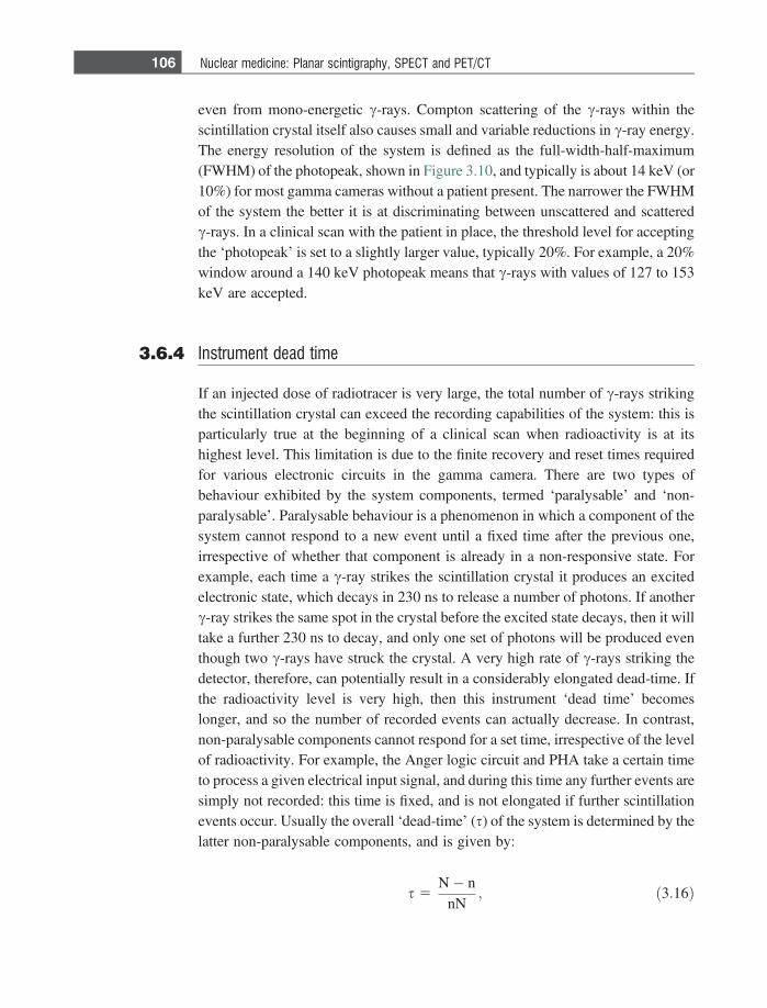
even from mono-energetic c-rays. Compton scattering of the c-rays within thescintillation crystal itself also causes small and variable reductions in c-ray energy.The energy resolution of the system is defined as the full-width-half-maximum(FWHM) of the photopeak, shown in Figure 3.10, and typically is about 14 keV (or10%) for most gamma cameras without a patient present. The narrower the FWHMof the system the better it is at discriminating between unscattered and scatteredc-rays. In a clinical scan with the patient in place, the threshold level for acceptingthe ‘photopeak’ is set to a slightly larger value, typically 20%. For example, a 20%window around a 140 keV photopeak means that c-rays with values of 127 to 153keV are accepted.
3.6.4 Instrument dead time
If an injected dose of radiotracer is very large, the total number of c-rays strikingthe scintillation crystal can exceed the recording capabilities of the system: this isparticularly true at the beginning of a clinical scan when radioactivity is at itshighest level. This limitation is due to the finite recovery and reset times requiredfor various electronic circuits in the gamma camera. There are two types ofbehaviour exhibited by the system components, termed ‘paralysable’ and ‘non-paralysable’. Paralysable behaviour is a phenomenon in which a component of thesystem cannot respond to a new event until a fixed time after the previous one,irrespective of whether that component is already in a non-responsive state. Forexample, each time a c-ray strikes the scintillation crystal it produces an excitedelectronic state, which decays in 230 ns to release a number of photons. If anotherc-ray strikes the same spot in the crystal before the excited state decays, then it willtake a further 230 ns to decay, and only one set of photons will be produced eventhough two c-rays have struck the crystal. A very high rate of c-rays striking thedetector, therefore, can potentially result in a considerably elongated dead-time. Ifthe radioactivity level is very high, then this instrument ‘dead time’ becomeslonger, and so the number of recorded events can actually decrease. In contrast,non-paralysable components cannot respond for a set time, irrespective of the levelof radioactivity. For example, the Anger logic circuit and PHA take a certain timeto process a given electrical input signal, and during this time any further events aresimply not recorded: this time is fixed, and is not elongated if further scintillationevents occur. Usually the overall ‘dead-time’ (s) of the system is determined by thelatter non-paralysable components, and is given by:
s 5N� n
nN; ð3:16Þ
106 Nuclear medicine: Planar scintigraphy, SPECT and PET/CT
where N is the true count rate (number of scintillations per second), and n is themeasured count rate. The maximum measurable count rate is given by 1/s.
Corrections for the dead-time are based upon calibrations using phantoms ofknown radioactivity, and also independent electronic measurements of the deadtime of individual components of the system. For example, Figure 3.11 shows aplot of measured count rate vs radioactivity from a calibrated source showing theasymptotic behaviour described by Equation (3.16). Experimentally, this type ofcurve can be produced by imaging a source with known radioactivity, andacquiring images at different time points as the source radioactivity decays (datapoints on the right of the graph at high count rates are acquired at the beginningof this experiment). This gives a calibration curve for correcting the acquiredimages.
Example 3.3 Suppose that the true count rate in a gamma camera is 10 000 per second, but themeasured rate is only 8000 per second. What is the dead time of the system?
Solution From Equation (3.16) the value of s is given as 25 ls. So rather than acquiring onecount every 100 ls (the true value), there is a 25 ls effective delay and one event isrecorded every 125 ls.
derusaemetar tnuoc
ytivitcaoidaR
detalopartxeetar eurt
etar tnuoC
Figure 3.11
Correction curve used to account for dead time losses. At very low count rates, the true rate andmeasured count rate are linearly related. As the radioactivity increases, the measured count ratereaches an asymptotic value, well below the true value.
107 3.6 The gamma camera
3.7 Image characteristics
Planar scintigraphy scans have no background signal since there is no natural c-rayemission from the body, and therefore the images have a high intrinsic contrast.However, a large proportion of emitted c-rays are scattered in the body and, if notremoved, would result in a significant random background signal which wouldreduce the image contrast. Therefore quite severe collimation is required, whichreduces the number of recorded events well below that of planar X-rays, forexample, and therefore the SNR is much lower. Collimation also introduces sig-nificant depth-dependent broadening, Equation (3.13), and the requirement forlow-pass filtering of the images due to the low SNR further degrades the spatialresolution.
Signal-to-noise
Since radioactive decay is a statistical process, in the sense that the spatial distri-bution of radioactivity at any one time does not have a single value but an averageone with associated standard deviation according to the Poisson distribution (Sec-tion 2.8.1), the image SNR is proportional to the square root of the total number ofdetected c-rays. This is exactly the same situation as for X-ray imaging. Factorsthat affect the SNR include:
(i) The amount of radiotracer administered, the time after administering theradiotracer at which imaging begins, the amount of radiotracer that accumu-lates in the organ being imaged, and the total time of the scan. Organs that aredeep within the patient, or on the opposite side to the planar detector willexperience more tissue attenuation of the c-rays, and therefore lower SNR,than organs closer to the detector.
(ii) The intrinsic sensitivity of the gamma camera. Since parameters that affect theSNR such as the crystal thickness are fixed, the only factors that can bechanged are the collimator properties (septal length, thickness and separation)and geometry (parallel, pinhole, converging or diverging).
(iii) Post-acquisition image filtering – due to the relatively low SNR of nuclearmedicine images, a low-pass filter is often applied to the image (see Section1.6). This filter increases the SNR but blurs the image, reducing the spatialresolution. The properties of the filter must be chosen carefully to maximizethe CNR.
Spatial resolution
The spatial resolution of the image is given by the combination of two majorinstrument components:
108 Nuclear medicine: Planar scintigraphy, SPECT and PET/CT
Rsystem 5
ffiffiffiffiffiffiffiffiffiffiffiffiffiffiffiffiffiffiffiffiffiffiffiffiffiffiffiffiffiR2
gamma 1 R2coll
q; ð3:17Þ
where Rgamma is the intrinsic spatial resolution of the gamma camera and Rcoll isdetermined by the collimator geometry. Contributions to Rgamma include the uncer-tainty in the exact location at which light is produced in the scintillation crystal,determined by the thickness of the crystal, and also the intrinsic resolution of theAnger position encoder (either analogue or digital). A typical value of Rgamma liesin the range 3–5 mm. The contribution from Rcoll depends upon the collimator typeand also the depth within the body of the organ in which the radiotracer accumu-lates, as seen in Equation (3.13). Typical values for the overall system spatialresolution are approximately 1–2 cm at large depths within the body, and 5–8mm close to the collimator surface.
Contrast and contrast-to-noise
The theoretical image contrast is extremely high in nuclear medicine since there isno background signal from tissues in which the radiotracer has not distributed.However, the presence of Compton scattered c-rays produces a random back-ground signal, with more scatter close to regions in which the radiotracer concen-trates. Factors affecting the spatial resolution also affect the contrast through the‘partial volume’ effect, in which image blurring causes signal ‘bleed’ from smallareas of high signal intensity to those where no radiotracer is present. The param-eters for low pass filtering of the final image must be chosen carefully since there isa compromise between too strong a filter reducing the contrast due to image blurand too weak a filter not reducing the noise sufficiently.
3.8 Clinical applications of planar scintigraphy
Over the past 20 years, the role of nuclear medicine in the clinic has changedsignificantly. For example, previous brain scanning has largely been replaced byPET, CT and MRI, and ventilation/perfusion scans are now largely performedusing multi-detector CT for evaluating pulmonary embolism. The major clinicalapplication of planar scintigraphy is whole-body bone scanning which constitutesabout 20% of all nuclear medicine scans. In addition, the thyroid, gastrointestinaltract, liver and kidneys are scanned using planar scintigraphy with specializedagents. For example, 99mTc can be attached to small particles of sulphur colloid,less than 100 nm diameter, which concentrate in healthy Kupffer cells in the liver,spleen and bone marrow. Pathological conditions such as cirrhosis of the liverresult in diseased Kupffer cells which can no longer uptake the radiotracer, andtherefore areas of low signal intensity, ‘cold spots’, are present in the image.
109 3.8 Clinical applications of planar scintigraphy
Bone scanning and tumour detection
Whole body scanning using 99mTc phosphonates such as hydroxymethylene-diphosphonate (HMDP, trade name Osteoscan) can be used to detect bonetumours, and also soft-tissue tumours which cause deformation and remodelingof bone structure. The mode of concentration of these agents in bone is thought toinvolve the affinity of diphosphonate for the metabolically active bone mineralhydroxyapatite, which exhibits increased metabolic turnover during bone growth.The usual response of bone to a tumour is to form new bone at the site of thetumour. For example, spinal tumours, which consist of metastatic lesions growingin the spinal marrow space, cause the bone structure of the spine to remodel. Thisresults in local uptake of the radiotracer. Scanning starts 2–3 hours after injectionof the radiotracer into a patient’s bloodstream to allow accumulation within theskeletal structure, and several scans with longitudinal overlap are used to cover thewhole body, as shown in Figure 3.12. If any suspected tumours are detected, thenfurther localized scans can be acquired. Bone infarctions or aggressive bone meta-stases often show up as signal voids in the nuclear medicine scan, since bonenecrosis has occurred and there is no blood flow to deliver the radiotracer to thatregion.
Other radiotracers which can be used in tumour detection are 67Ga-citrate and201Tl. Radiotracer ligands can also be designed for active targetting of specifictumours which are known to express certain receptors. For example, 111In-DTPA-octreotide has been designed to target tumours which over-express somatostatinreceptors.
3.9 Single photon emission computed tomography (SPECT)
SPECT uses two or three gamma cameras which rotate around the patient detectingc-rays at a number of different angles. Either filtered backprojection or iterativetechniques are used to reconstruct multiple two-dimensional axial slices from theacquired projections. The relationship between planar scintigraphy and SPECT isanalogous to that between planar X-ray imaging and CT. SPECT uses essentiallythe same instrumentation and many of the same radiotracers as planar scintigraphy,and most SPECT machines can also be used for planar scans. The majority ofSPECT scans are used for myocardial perfusion studies to detect coronary arterydisease or myocardial infarction, although SPECT is also used for brain studies todetect areas of reduced blood flow associated with stroke, epilepsy or neurodege-nerative diseases such as Alzheimers.
Since the array of PMTs is two-dimensional in nature, the data can be recon-structed as a series of adjacent slices, as shown in Figure 3.13. A 360� rotation is
110 Nuclear medicine: Planar scintigraphy, SPECT and PET/CT
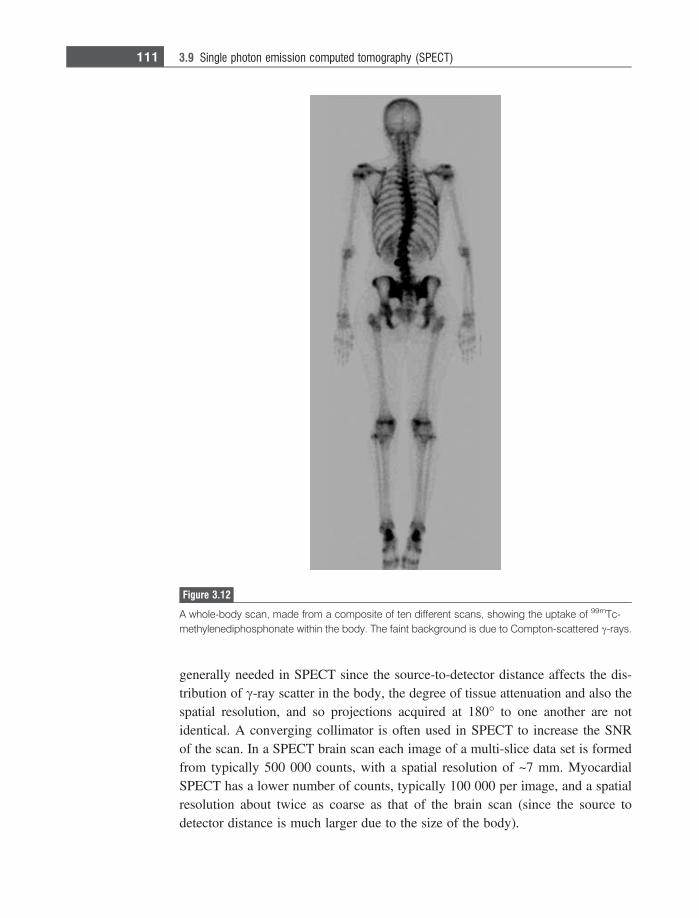
generally needed in SPECT since the source-to-detector distance affects the dis-tribution of c-ray scatter in the body, the degree of tissue attenuation and also thespatial resolution, and so projections acquired at 180� to one another are notidentical. A converging collimator is often used in SPECT to increase the SNRof the scan. In a SPECT brain scan each image of a multi-slice data set is formedfrom typically 500 000 counts, with a spatial resolution of ~7 mm. MyocardialSPECT has a lower number of counts, typically 100 000 per image, and a spatialresolution about twice as coarse as that of the brain scan (since the source todetector distance is much larger due to the size of the body).
Figure 3.12
A whole-body scan, made from a composite of ten different scans, showing the uptake of 99mTc-methylenediphosphonate within the body. The faint background is due to Compton-scattered c-rays.
111 3.9 Single photon emission computed tomography (SPECT)
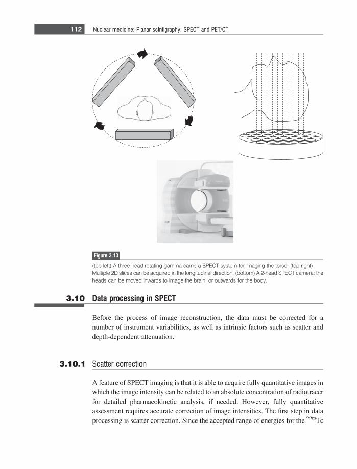
3.10 Data processing in SPECT
Before the process of image reconstruction, the data must be corrected for anumber of instrument variabilities, as well as intrinsic factors such as scatter anddepth-dependent attenuation.
3.10.1 Scatter correction
A feature of SPECT imaging is that it is able to acquire fully quantitative images inwhich the image intensity can be related to an absolute concentration of radiotracerfor detailed pharmacokinetic analysis, if needed. However, fully quantitativeassessment requires accurate correction of image intensities. The first step in dataprocessing is scatter correction. Since the accepted range of energies for the 99mTc
Figure 3.13
(top left) A three-head rotating gamma camera SPECT system for imaging the torso. (top right)Multiple 2D slices can be acquired in the longitudinal direction. (bottom) A 2-head SPECT camera: theheads can be moved inwards to image the brain, or outwards for the body.
112 Nuclear medicine: Planar scintigraphy, SPECT and PET/CT
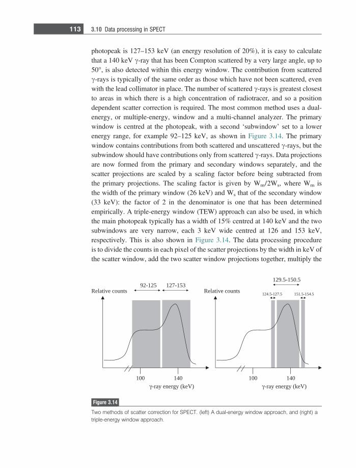
photopeak is 127–153 keV (an energy resolution of 20%), it is easy to calculatethat a 140 keV c-ray that has been Compton scattered by a very large angle, up to50�, is also detected within this energy window. The contribution from scatteredc-rays is typically of the same order as those which have not been scattered, evenwith the lead collimator in place. The number of scattered c-rays is greatest closestto areas in which there is a high concentration of radiotracer, and so a positiondependent scatter correction is required. The most common method uses a dual-energy, or multiple-energy, window and a multi-channel analyzer. The primarywindow is centred at the photopeak, with a second ‘subwindow’ set to a lowerenergy range, for example 92–125 keV, as shown in Figure 3.14. The primarywindow contains contributions from both scattered and unscattered c-rays, but thesubwindow should have contributions only from scattered c-rays. Data projectionsare now formed from the primary and secondary windows separately, and thescatter projections are scaled by a scaling factor before being subtracted fromthe primary projections. The scaling factor is given by Wm/2Ws, where Wm isthe width of the primary window (26 keV) and Ws that of the secondary window(33 keV): the factor of 2 in the denominator is one that has been determinedempirically. A triple-energy window (TEW) approach can also be used, in whichthe main photopeak typically has a width of 15% centred at 140 keV and the twosubwindows are very narrow, each 3 keV wide centred at 126 and 153 keV,respectively. This is also shown in Figure 3.14. The data processing procedureis to divide the counts in each pixel of the scatter projections by the width in keV ofthe scatter window, add the two scatter window projections together, multiply the
041001 041001
stnuoc evitaleR
)Vek( ygrene yar-
351-721521-29stnuoc evitaleR
)Vek( ygrene yar-
5.721-5.421
5.051-5.921
5.451-5.151
Figure 3.14
Two methods of scatter correction for SPECT. (left) A dual-energy window approach, and (right) atriple-energy window approach.
113 3.10 Data processing in SPECT
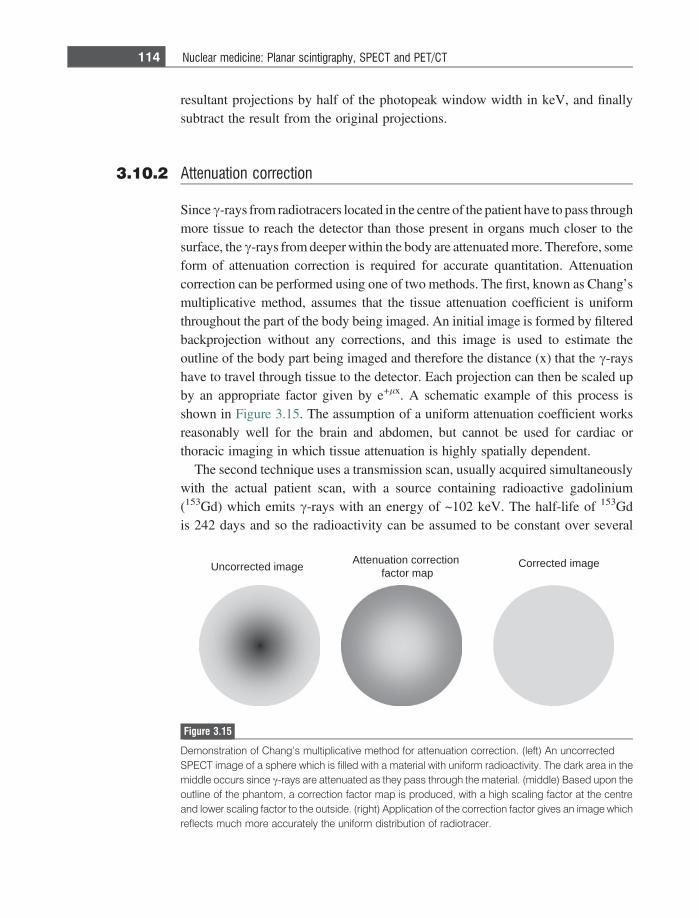
resultant projections by half of the photopeak window width in keV, and finallysubtract the result from the original projections.
3.10.2 Attenuation correction
Since c-rays from radiotracers located in the centre of the patient have to pass throughmore tissue to reach the detector than those present in organs much closer to thesurface, the c-rays from deeper within the body are attenuated more. Therefore, someform of attenuation correction is required for accurate quantitation. Attenuationcorrection can be performed using one of two methods. The first, known as Chang’smultiplicative method, assumes that the tissue attenuation coefficient is uniformthroughout the part of the body being imaged. An initial image is formed by filteredbackprojection without any corrections, and this image is used to estimate theoutline of the body part being imaged and therefore the distance (x) that the c-rayshave to travel through tissue to the detector. Each projection can then be scaled upby an appropriate factor given by e+lx. A schematic example of this process isshown in Figure 3.15. The assumption of a uniform attenuation coefficient worksreasonably well for the brain and abdomen, but cannot be used for cardiac orthoracic imaging in which tissue attenuation is highly spatially dependent.
The second technique uses a transmission scan, usually acquired simultaneouslywith the actual patient scan, with a source containing radioactive gadolinium(153Gd) which emits c-rays with an energy of ~102 keV. The half-life of 153Gdis 242 days and so the radioactivity can be assumed to be constant over several
Uncorrected image Attenuation correction factor map
Corrected image
Figure 3.15
Demonstration of Chang’s multiplicative method for attenuation correction. (left) An uncorrectedSPECT image of a sphere which is filled with a material with uniform radioactivity. The dark area in themiddle occurs since c-rays are attenuated as they pass through the material. (middle) Based upon theoutline of the phantom, a correction factor map is produced, with a high scaling factor at the centreand lower scaling factor to the outside. (right) Application of the correction factor gives an image whichreflects much more accurately the uniform distribution of radiotracer.
114 Nuclear medicine: Planar scintigraphy, SPECT and PET/CT
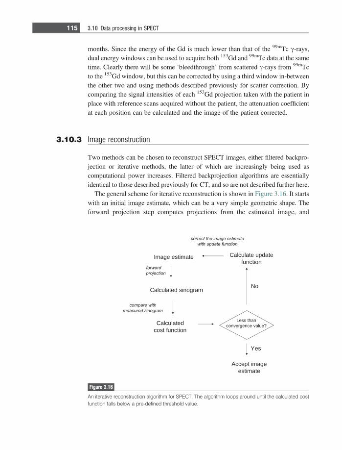
months. Since the energy of the Gd is much lower than that of the 99mTc c-rays,dual energy windows can be used to acquire both 153Gd and 99mTc data at the sametime. Clearly there will be some ‘bleedthrough’ from scattered c-rays from 99mTcto the 153Gd window, but this can be corrected by using a third window in-betweenthe other two and using methods described previously for scatter correction. Bycomparing the signal intensities of each 153Gd projection taken with the patient inplace with reference scans acquired without the patient, the attenuation coefficientat each position can be calculated and the image of the patient corrected.
3.10.3 Image reconstruction
Two methods can be chosen to reconstruct SPECT images, either filtered backpro-jection or iterative methods, the latter of which are increasingly being used ascomputational power increases. Filtered backprojection algorithms are essentiallyidentical to those described previously for CT, and so are not described further here.
The general scheme for iterative reconstruction is shown in Figure 3.16. It startswith an initial image estimate, which can be a very simple geometric shape. Theforward projection step computes projections from the estimated image, and
etamitse egamI
drawrof
noitcejorp
margonis detaluclaC
htiw erapmoc
margonis derusaem
detaluclaCnoitcnuf tsoc
naht sseL?eulav ecnegrevnoc
seY
egami tpeccAetamitse
oN
etadpu etaluclaCnoitcnuf
mi eht tcerroc etamitse ega
noitcnuf etadpu htiw
Figure 3.16
An iterative reconstruction algorithm for SPECT. The algorithm loops around until the calculated costfunction falls below a pre-defined threshold value.
115 3.10 Data processing in SPECT
assembles them into a sinogram. During this process, estimates of the distributionof scattered c-rays, spatially-dependent attenuation and a depth-dependent pointspread function can be built into the forward model. The sinogram is then com-pared with the one that is actually acquired, and the difference between the two iscalculated as a cost function. This cost function can be a simple sum-of-squaresdifference between the actual and predicted data on a pixel-by-pixel basis, or canweight more heavily the areas of the sinogram which have the highest signalintensity. Based upon the cost function the estimated data are now updated toimprove the similarity between actual and estimated data. There are a number ofpossible update functions, and the appropriate choice is an active area of mathe-matical development. Since there is never perfect agreement between the measuredand estimated sinograms, a lower threshold value of the cost function, which isdetermined to be acceptable, is defined (alternatively the total number of iterationscan be given a maximum value). At each stage of the iteration, this calculated costfunction is compared with this threshold. If it is above the threshold, i.e. thereconstruction is not ‘good enough’, then the estimated image is recalculated usingan update function based upon the error. Iterative reconstruction is a very computa-tionally intensive process, and there are a number of methods that have beendevised to speed it up. One general class is termed ‘ordered subsets’, in whichthe early iterative stages use only a small subset of the acquired profiles, with thisnumber increasing to the full amount as the iteration progresses. The most commonalgorithm used is referred to as the maximum-likelihood expectation-maximum(ML-EM) method.
3.11 SPECT/CT
Since 2005 there has been an increasing trend to combine SPECT with CT in acombined scanner [2;3]. In 2008 there were approximately 1000 SPECT/CT systemsinstalled worldwide. A SPECT/CT system acquires data from the two image modal-ities with a single integrated patient bed and gantry. The two imaging studies areperformed with the patient remaining on the table, which is moved from the CTscanner to the SPECT system, as shown in Figure 3.17. Typical clinical systems usea two-head SPECT camera with a multi-slice CT scanner. The primary advantagesof a combined SPECT/CT over a stand-alone SPECT system are: (i) improvedattenuation correction for SPECT reconstruction using the high resolution anatom-ical information from the CT scanner, and (ii) the fusion of high-resolution anatom-ical (CT) with functional (SPECT) information, allowing the anatomical location ofradioactive ‘hot’ or ‘cold’ spots to be defined much better with reduced partialvolume effects compared to SPECT alone. In terms of the advantages of CT-based
116 Nuclear medicine: Planar scintigraphy, SPECT and PET/CT
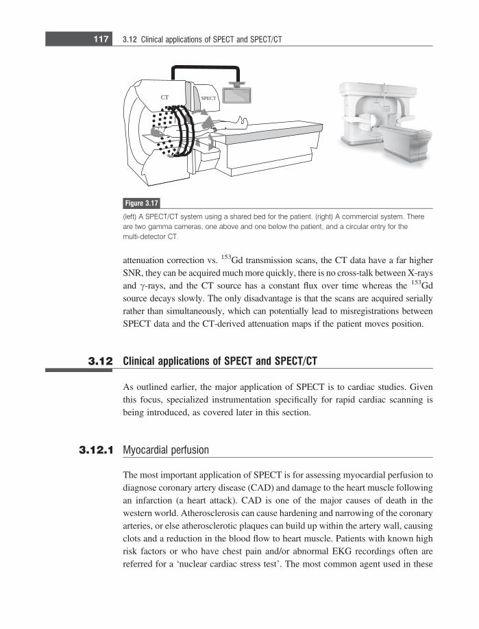
attenuation correction vs. 153Gd transmission scans, the CT data have a far higherSNR, they can be acquired much more quickly, there is no cross-talk between X-raysand c-rays, and the CT source has a constant flux over time whereas the 153Gdsource decays slowly. The only disadvantage is that the scans are acquired seriallyrather than simultaneously, which can potentially lead to misregistrations betweenSPECT data and the CT-derived attenuation maps if the patient moves position.
3.12 Clinical applications of SPECT and SPECT/CT
As outlined earlier, the major application of SPECT is to cardiac studies. Giventhis focus, specialized instrumentation specifically for rapid cardiac scanning isbeing introduced, as covered later in this section.
3.12.1 Myocardial perfusion
The most important application of SPECT is for assessing myocardial perfusion todiagnose coronary artery disease (CAD) and damage to the heart muscle followingan infarction (a heart attack). CAD is one of the major causes of death in thewestern world. Atherosclerosis can cause hardening and narrowing of the coronaryarteries, or else atherosclerotic plaques can build up within the artery wall, causingclots and a reduction in the blood flow to heart muscle. Patients with known highrisk factors or who have chest pain and/or abnormal EKG recordings often arereferred for a ‘nuclear cardiac stress test’. The most common agent used in these
SPECTCT
Figure 3.17
(left) A SPECT/CT system using a shared bed for the patient. (right) A commercial system. Thereare two gamma cameras, one above and one below the patient, and a circular entry for themulti-detector CT.
117 3.12 Clinical applications of SPECT and SPECT/CT
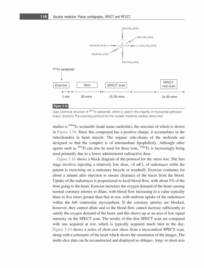
studies is 99mTc-sestamibi (trade name cardiolite), the structure of which is shownin Figure 3.18. Since this compound has a positive charge, it accumulates in themitochondria in heart muscle. The organic side-chains of the molecule aredesigned so that the complex is of intermediate lipophilicity. Although otheragents such as 201Tl can also be used for these tests, 99mTc is increasingly beingused primarily due to a lower administered radioactive dose.
Figure 3.18 shows a block diagram of the protocol for the stress test. The firststage involves injecting a relatively low dose, ~8 mCi, of radiotracer while thepatient is exercising on a stationary bicycle or treadmill. Exercise continues forabout a minute after injection to ensure clearance of the tracer from the blood.Uptake of the radiotracer is proportional to local blood flow, with about 5% of thedose going to the heart. Exercise increases the oxygen demand of the heart causingnormal coronary arteries to dilate, with blood flow increasing to a value typicallythree to five times greater than that at rest, with uniform uptake of the radiotracerwithin the left ventricular myocardium. If the coronary arteries are blocked,however, they cannot dilate and so the blood flow cannot increase sufficiently tosatisfy the oxygen demand of the heart, and this shows up as an area of low signalintensity on the SPECT scan. The results of this first SPECT scan are comparedwith one acquired at rest, which is typically acquired much later in the day.Figure 3.19 shows a series of short-axis slices from a myocardical SPECT scan,along with a schematic of the heart which shows the orientation of the images. Themulti-slice data can be reconstructed and displayed as oblique-, long- or short-axis
Exercise
99mTc-sestamibi
1 min
Rest SPECT scan
30 mins 15-30 mins
...............
SPECTrest scan
15-30 mins
Figure 3.18
(top) Chemical structure of 99mTc-sestamibi, which is used in the majority of myocardial perfusionscans. (bottom) The scanning protocol for the nuclear medicine cardiac stress test.
118 Nuclear medicine: Planar scintigraphy, SPECT and PET/CT
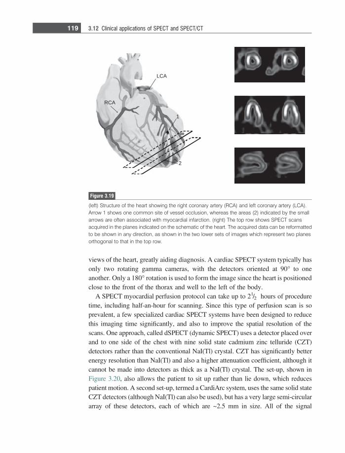
views of the heart, greatly aiding diagnosis. A cardiac SPECT system typically hasonly two rotating gamma cameras, with the detectors oriented at 90� to oneanother. Only a 180� rotation is used to form the image since the heart is positionedclose to the front of the thorax and well to the left of the body.
A SPECT myocardial perfusion protocol can take up to 21/2 hours of proceduretime, including half-an-hour for scanning. Since this type of perfusion scan is soprevalent, a few specialized cardiac SPECT systems have been designed to reducethis imaging time significantly, and also to improve the spatial resolution of thescans. One approach, called dSPECT (dynamic SPECT) uses a detector placed overand to one side of the chest with nine solid state cadmium zinc telluride (CZT)detectors rather than the conventional NaI(Tl) crystal. CZT has significantly betterenergy resolution than NaI(Tl) and also a higher attenuation coefficient, although itcannot be made into detectors as thick as a NaI(Tl) crystal. The set-up, shown inFigure 3.20, also allows the patient to sit up rather than lie down, which reducespatient motion. A second set-up, termed a CardiArc system, uses the same solid stateCZT detectors (although NaI(Tl) can also be used), but has a very large semi-circulararray of these detectors, each of which are ~2.5 mm in size. All of the signal
LCA
RCA
1
2
Figure 3.19
(left) Structure of the heart showing the right coronary artery (RCA) and left coronary artery (LCA).Arrow 1 shows one common site of vessel occlusion, whereas the areas (2) indicated by the smallarrows are often associated with myocardial infarction. (right) The top row shows SPECT scansacquired in the planes indicated on the schematic of the heart. The acquired data can be reformattedto be shown in any direction, as shown in the two lower sets of images which represent two planesorthogonal to that in the top row.
119 3.12 Clinical applications of SPECT and SPECT/CT
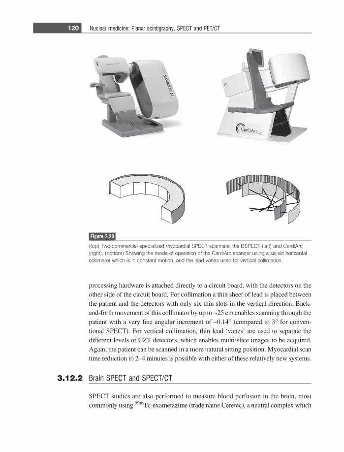
processing hardware is attached directly to a circuit board, with the detectors on theother side of the circuit board. For collimation a thin sheet of lead is placed betweenthe patient and the detectors with only six thin slots in the vertical direction. Back-and-forth movement of this collimator by up to ~25 cm enables scanning through thepatient with a very fine angular increment of ~0.14� (compared to 3� for conven-tional SPECT). For vertical collimation, thin lead ‘vanes’ are used to separate thedifferent levels of CZT detectors, which enables multi-slice images to be acquired.Again, the patient can be scanned in a more natural sitting position. Myocardial scantime reduction to 2–4 minutes is possible with either of these relatively new systems.
3.12.2 Brain SPECT and SPECT/CT
SPECT studies are also performed to measure blood perfusion in the brain, mostcommonly using 99mTc-exametazime (trade name Ceretec), a neutral complex which
Figure 3.20
(top) Two commercial specialized myocardial SPECT scanners, the DSPECT (left) and CardiArc(right). (bottom) Showing the mode of operation of the CardiArc scanner using a six-slit horizontalcollimator which is in constant motion, and the lead vanes used for vertical collimation.
120 Nuclear medicine: Planar scintigraphy, SPECT and PET/CT
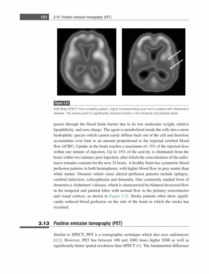
passes through the blood brain barrier due to its low molecular weight, relativelipophilicity, and zero charge. The agent is metabolized inside the cells into a morehydrophilic species which cannot easily diffuse back out of the cell and thereforeaccumulates over time to an amount proportional to the regional cerebral bloodflow (rCBF). Uptake in the brain reaches a maximum of ~5% of the injected dosewithin one minute of injection. Up to 15% of the activity is eliminated from thebrain within two minutes post-injection, after which the concentration of the radio-tracer remains constant for the next 24 hours. A healthy brain has symmetric bloodperfusion patterns in both hemispheres, with higher blood flow in grey matter thanwhite matter. Diseases which cause altered perfusion patterns include epilepsy,cerebral infarction, schizophrenia and dementia. One commonly studied form ofdementia is Alzheimer’s disease, which is characterized by bilateral decreased flowin the temporal and parietal lobes with normal flow in the primary sensorimotorand visual cortices, as shown in Figure 3.21. Stroke patients often show signifi-cantly reduced blood perfusion on the side of the brain in which the stroke hasoccurred.
3.13 Positron emission tomography (PET)
Similar to SPECT, PET is a tomographic technique which also uses radiotracers[4;5]. However, PET has between 100 and 1000 times higher SNR as well assignificantly better spatial resolution than SPECT (6). The fundamental difference
Figure 3.21
(left) Brain SPECT from a healthy patient. (right) Corresponding scan from a patient with Alzheimer’sdisease. The arrows point to significantly reduced activity in the temporal and parietal lobes.
121 3.13 Positron emission tomography (PET)
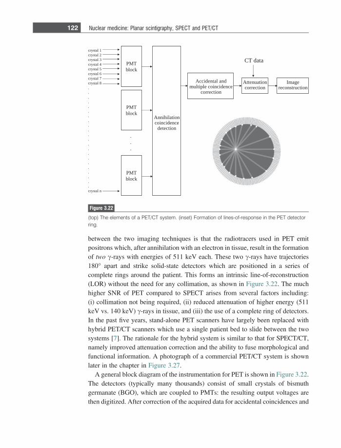
between the two imaging techniques is that the radiotracers used in PET emitpositrons which, after annihilation with an electron in tissue, result in the formationof two c-rays with energies of 511 keV each. These two c-rays have trajectories180� apart and strike solid-state detectors which are positioned in a series ofcomplete rings around the patient. This forms an intrinsic line-of-reconstruction(LOR) without the need for any collimation, as shown in Figure 3.22. The muchhigher SNR of PET compared to SPECT arises from several factors including:(i) collimation not being required, (ii) reduced attenuation of higher energy (511keV vs. 140 keV) c-rays in tissue, and (iii) the use of a complete ring of detectors.In the past five years, stand-alone PET scanners have largely been replaced withhybrid PET/CT scanners which use a single patient bed to slide between the twosystems [7]. The rationale for the hybrid system is similar to that for SPECT/CT,namely improved attenuation correction and the ability to fuse morphological andfunctional information. A photograph of a commercial PET/CT system is shownlater in the chapter in Figure 3.27.
A general block diagram of the instrumentation for PET is shown in Figure 3.22.The detectors (typically many thousands) consist of small crystals of bismuthgermanate (BGO), which are coupled to PMTs: the resulting output voltages arethen digitized. After correction of the acquired data for accidental coincidences and
1latsyrc2latsyrc3latsyrc4latsyrc5latsyrc6latsyrc7latsyrc8latsyrc
.
.
.
.
.
.
.
.
.
.
.
.
.
.
.
.
.
.
.
.
.
.nlatsyrc
TMPkcolb
TMPkcolb
noitalihinnAecnedicnioc
noitceted
dnalatnediccAecnedicniocelpitlum
noitcerroc
noitaunettAnoitcerroc
egamInoitcurtsnocer
atadTC
.
.
.
TMPkcolb
Figure 3.22
(top) The elements of a PET/CT system. (inset) Formation of lines-of-response in the PET detectorring.
122 Nuclear medicine: Planar scintigraphy, SPECT and PET/CT
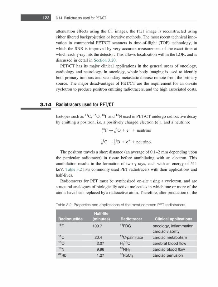
attenuation effects using the CT images, the PET image is reconstructed usingeither filtered backprojection or iterative methods. The most recent technical inno-vation in commercial PET/CT scanners is time-of-flight (TOF) technology, inwhich the SNR is improved by very accurate measurement of the exact time atwhich each c-ray hits the detector. This allows localization within the LOR, and isdiscussed in detail in Section 3.20.
PET/CT has its major clinical applications in the general areas of oncology,cardiology and neurology. In oncology, whole body imaging is used to identifyboth primary tumours and secondary metastatic disease remote from the primarysource. The major disadvantages of PET/CT are the requirement for an on-sitecyclotron to produce positron emitting radiotracers, and the high associated costs.
3.14 Radiotracers used for PET/CT
Isotopes such as 11C, 15O, 18F and 13N used in PET/CT undergo radioactive decayby emitting a positron, i.e. a positively charged electron (e+), and a neutrino:
189 F! 18
8 O 1 e1 1 neutrino
116 C! 11
5 B 1 e1 1 neutrino:
The positron travels a short distance (an average of 0.1–2 mm depending uponthe particular radiotracer) in tissue before annihilating with an electron. Thisannihilation results in the formation of two c-rays, each with an energy of 511keV. Table 3.2 lists commonly used PET radiotracers with their applications andhalf-lives.
Radiotracers for PET must be synthesized on-site using a cyclotron, and arestructural analogues of biologically active molecules in which one or more of theatoms have been replaced by a radioactive atom. Therefore, after production of the
Table 3.2: Properties and applications of the most common PET radiotracers
RadionuclideHalf-life
(minutes) Radiotracer Clinical applications18F 109.7 18FDG oncology, inflammation,
cardiac viability11C 20.4 11C-palmitate cardiac metabolism15O 2.07 H2
15O cerebral blood flow13N 9.96 13NH3 cardiac blood flow82Rb 1.27 82RbCl2 cardiac perfusion
123 3.14 Radiotracers used for PET/CT
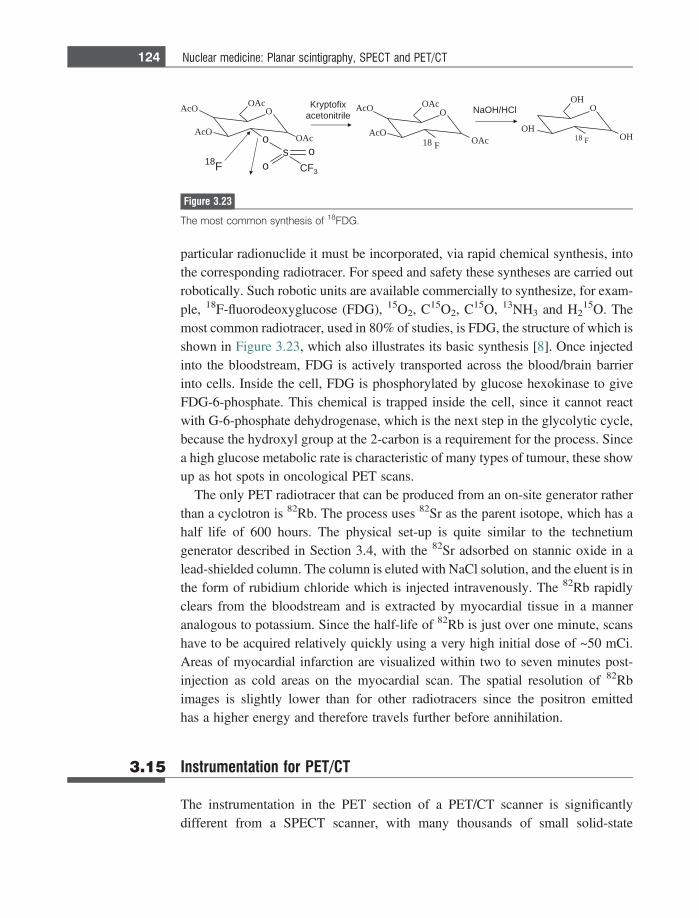
particular radionuclide it must be incorporated, via rapid chemical synthesis, intothe corresponding radiotracer. For speed and safety these syntheses are carried outrobotically. Such robotic units are available commercially to synthesize, for exam-ple, 18F-fluorodeoxyglucose (FDG), 15O2, C15O2, C15O, 13NH3 and H2
15O. Themost common radiotracer, used in 80% of studies, is FDG, the structure of which isshown in Figure 3.23, which also illustrates its basic synthesis [8]. Once injectedinto the bloodstream, FDG is actively transported across the blood/brain barrierinto cells. Inside the cell, FDG is phosphorylated by glucose hexokinase to giveFDG-6-phosphate. This chemical is trapped inside the cell, since it cannot reactwith G-6-phosphate dehydrogenase, which is the next step in the glycolytic cycle,because the hydroxyl group at the 2-carbon is a requirement for the process. Sincea high glucose metabolic rate is characteristic of many types of tumour, these showup as hot spots in oncological PET scans.
The only PET radiotracer that can be produced from an on-site generator ratherthan a cyclotron is 82Rb. The process uses 82Sr as the parent isotope, which has ahalf life of 600 hours. The physical set-up is quite similar to the technetiumgenerator described in Section 3.4, with the 82Sr adsorbed on stannic oxide in alead-shielded column. The column is eluted with NaCl solution, and the eluent is inthe form of rubidium chloride which is injected intravenously. The 82Rb rapidlyclears from the bloodstream and is extracted by myocardial tissue in a manneranalogous to potassium. Since the half-life of 82Rb is just over one minute, scanshave to be acquired relatively quickly using a very high initial dose of ~50 mCi.Areas of myocardial infarction are visualized within two to seven minutes post-injection as cold areas on the myocardial scan. The spatial resolution of 82Rbimages is slightly lower than for other radiotracers since the positron emittedhas a higher energy and therefore travels further before annihilation.
3.15 Instrumentation for PET/CT
The instrumentation in the PET section of a PET/CT scanner is significantlydifferent from a SPECT scanner, with many thousands of small solid-state
O
HO
HO
81 F HO
O
OcA
cAO
81 F cAO
OcAO
OcA
cAO
cAO
OcA
os
ooFC 3
81 F
lCH/HOaNxifotpyrKelirtinoteca
Figure 3.23
The most common synthesis of 18FDG.
124 Nuclear medicine: Planar scintigraphy, SPECT and PET/CT
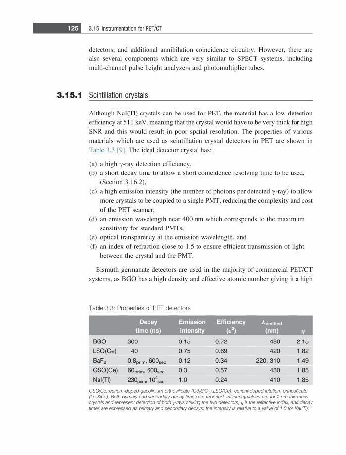
detectors, and additional annihilation coincidence circuitry. However, there arealso several components which are very similar to SPECT systems, includingmulti-channel pulse height analyzers and photomultiplier tubes.
3.15.1 Scintillation crystals
Although NaI(Tl) crystals can be used for PET, the material has a low detectionefficiency at 511 keV, meaning that the crystal would have to be very thick for highSNR and this would result in poor spatial resolution. The properties of variousmaterials which are used as scintillation crystal detectors in PET are shown inTable 3.3 [9]. The ideal detector crystal has:
(a) a high c-ray detection efficiency,(b) a short decay time to allow a short coincidence resolving time to be used,
(Section 3.16.2),(c) a high emission intensity (the number of photons per detected c-ray) to allow
more crystals to be coupled to a single PMT, reducing the complexity and costof the PET scanner,
(d) an emission wavelength near 400 nm which corresponds to the maximumsensitivity for standard PMTs,
(e) optical transparency at the emission wavelength, and(f) an index of refraction close to 1.5 to ensure efficient transmission of light
between the crystal and the PMT.
Bismuth germanate detectors are used in the majority of commercial PET/CTsystems, as BGO has a high density and effective atomic number giving it a high
Table 3.3: Properties of PET detectors
Decaytime (ns)
Emissionintensity
Efficiency(e2)
lemitted
(nm) h
BGO 300 0.15 0.72 480 2.15
LSO(Ce) 40 0.75 0.69 420 1.82
BaF2 0.8prim, 600sec 0.12 0.34 220, 310 1.49
GSO(Ce) 60prim, 600sec 0.3 0.57 430 1.85
NaI(Tl) 230prim, 104sec 1.0 0.24 410 1.85
GSO(Ce):cerium-doped gadolinium orthosilicate (Gd2SiO5),LSO(Ce): cerium-doped lutetium orthosilicate(Lu2SiO5). Both primary and secondary decay times are reported, efficiency values are for 2 cm thicknesscrystals and represent detection of both c-rays striking the two detectors, g is the refractive index, and decaytimes are expressed as primary and secondary decays; the intensity is relative to a value of 1.0 for NaI(Tl).
125 3.15 Instrumentation for PET/CT
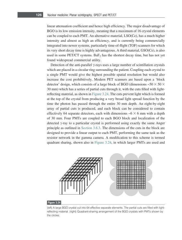
linear attenuation coefficient and hence high efficiency. The major disadvantage ofBGO is its low emission intensity, meaning that a maximum of 16 crystal elementscan be coupled to each PMT. An alternative material, LSO(Ce), has a much higherintensity and almost as high an efficiency, and is currently being commerciallyintegrated into newer systems, particularly time-of-flight (TOF) scanners for whichits very short decay time is highly advantageous. A third material, GSO(Ce), is alsoused in some PET/CT systems. BaF2 has the shortest decay time, but has not yetfound widespread commercial utility.
Detection of the anti-parallel c-rays uses a large number of scintillation crystalswhich are placed in a circular ring surrounding the patient. Coupling each crystal toa single PMT would give the highest possible spatial resolution but would alsoincrease the cost prohibitively. Modern PET scanners are based upon a ‘blockdetector’ design, which consists of a large block of BGO (dimensions ~50 3 50 3
30 mm) which has a series of partial cuts through it, with the cuts filled with light-reflecting material, as shown in Figure 3.24. The cuts prevent light which is formedat the top of the crystal from producing a very broad light spread function by thetime the photon has passed through the entire 30 mm depth. An eight-by-eightarray of partial cuts is produced, and each block can be considered to containeffectively 64 separate detectors, each with dimensions ~6 3 6 mm with a depthof 30 mm. Four PMTs are coupled to each BGO block and localization of thedetected c-ray to a particular crystal is performed using exactly the same Angerprinciple as outlined in Section 3.6.3. The dimensions of the cuts in the block aredesigned to provide a linear output to each PMT, performing the same task as theresistor network in the gamma camera. A modification to this scheme is termedquadrant sharing, shown also in Figure 3.24, in which larger PMTs are used and
Figure 3.24
(left) A large BGO crystal cut into 64 effective separate elements. The partial cuts are filled with light-reflecting material. (right) Quadrant-sharing arrangement of the BGO crystals with PMTs shown bythe circles.
126 Nuclear medicine: Planar scintigraphy, SPECT and PET/CT
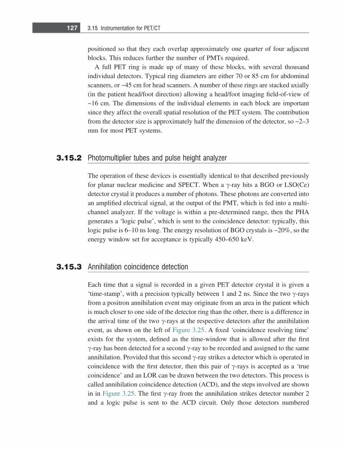
positioned so that they each overlap approximately one quarter of four adjacentblocks. This reduces further the number of PMTs required.
A full PET ring is made up of many of these blocks, with several thousandindividual detectors. Typical ring diameters are either 70 or 85 cm for abdominalscanners, or ~45 cm for head scanners. A number of these rings are stacked axially(in the patient head/foot direction) allowing a head/foot imaging field-of-view of~16 cm. The dimensions of the individual elements in each block are importantsince they affect the overall spatial resolution of the PET system. The contributionfrom the detector size is approximately half the dimension of the detector, so ~2–3mm for most PET systems.
3.15.2 Photomultiplier tubes and pulse height analyzer
The operation of these devices is essentially identical to that described previouslyfor planar nuclear medicine and SPECT. When a c-ray hits a BGO or LSO(Ce)detector crystal it produces a number of photons. These photons are converted intoan amplified electrical signal, at the output of the PMT, which is fed into a multi-channel analyzer. If the voltage is within a pre-determined range, then the PHAgenerates a ‘logic pulse’, which is sent to the coincidence detector: typically, thislogic pulse is 6–10 ns long. The energy resolution of BGO crystals is ~20%, so theenergy window set for acceptance is typically 450–650 keV.
3.15.3 Annihilation coincidence detection
Each time that a signal is recorded in a given PET detector crystal it is given a‘time-stamp’, with a precision typically between 1 and 2 ns. Since the two c-raysfrom a positron annihilation event may originate from an area in the patient whichis much closer to one side of the detector ring than the other, there is a difference inthe arrival time of the two c-rays at the respective detectors after the annihilationevent, as shown on the left of Figure 3.25. A fixed ‘coincidence resolving time’exists for the system, defined as the time-window that is allowed after the firstc-ray has been detected for a second c-ray to be recorded and assigned to the sameannihilation. Provided that this second c-ray strikes a detector which is operated incoincidence with the first detector, then this pair of c-rays is accepted as a ‘truecoincidence’ and an LOR can be drawn between the two detectors. This process iscalled annihilation coincidence detection (ACD), and the steps involved are shownin in Figure 3.25. The first c-ray from the annihilation strikes detector number 2and a logic pulse is sent to the ACD circuit. Only those detectors numbered
127 3.15 Instrumentation for PET/CT
between 7 and 13 are ‘in coincidence’ with detector number 2 since unscatteredc-rays which originate from within the head must lie within the volume defined bydetectors 7–13, as shown in Figure 3.25. When the second c-ray is detected incrystal 10 a second logic pulse is sent to the ACD circuit, which adds the twopulses together. If the summed signal is greater than a threshold set to a value justless than twice the amplitude of each individual logic pulse, then a coincidence isaccepted and an LOR established between the two detectors. The coincidenceresolving time is defined as twice the length of each logic pulse, with a valuetypically between 6 and 12 ns.
Example 3.4 Assume that the head is an ellipse with major dimensions 28 and 22 cm. Thepatient is placed within a head PET scanner with a circular arrangement, diameter45 cm, of BGO detectors. What is the maximum time difference that can occur foran event between two detectors?
Solution The maximum difference clearly corresponds to a scintillation event occurringeither right at the front or at the back of the head. Assuming that the head isperfectly centred in the PET scanner, there is a 28 cm difference in the trajectoriesof the two c-rays. Assuming that the c-rays travel through tissue at the speedof light, 3 3 108 m/s, then the times of detection will be ~930 ps, or just less than1 ns apart.
2789
01112131
emit
demmuSlangis
12
3
4
5
6
789
01
11
21
31
5161
41
Figure 3.25
The principle of annihilation coincidence detection. (left) The two c-rays reach detectors 2 and 10,triggering respective logic pulses of length s. (right) If both logic pulses are sent to the coincidencedetector within the system coincidence resolving time 2s, then the summed signal lies above thethreshold value (dashed line) and a coincidence is recorded.
128 Nuclear medicine: Planar scintigraphy, SPECT and PET/CT
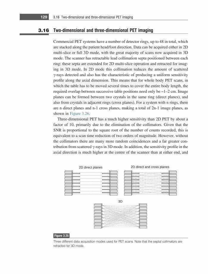
3.16 Two-dimensional and three-dimensional PET imaging
Commercial PET systems have a number of detector rings, up to 48 in total, whichare stacked along the patient head/foot direction. Data can be acquired either in 2Dmulti-slice or full 3D mode, with the great majority of scans now acquired in 3Dmode. The scanner has retractable lead collimation septa positioned between eachring: these septa are extended for 2D multi-slice operation and retracted for imag-ing in 3D mode. In 2D mode this collimation reduces the amount of scatteredc-rays detected and also has the characteristic of producing a uniform sensitivityprofile along the axial dimension. This means that for whole body PET scans, inwhich the table has to be moved several times to cover the entire body length, therequired overlap between successive table positions need only be ~1–2 cm. Imageplanes can be formed between two crystals in the same ring (direct planes), andalso from crystals in adjacent rings (cross planes). For a system with n rings, thereare n direct planes and n-1 cross planes, making a total of 2n-1 image planes, asshown in Figure 3.26.
Three-dimensional PET has a much higher sensitivity than 2D PET by about afactor of 10, primarily due to the elimination of the collimators. Given that theSNR is proportional to the square root of the number of counts recorded, this isequivalent to a scan time reduction of two orders of magnitude. However, withoutthe collimators there are many more random coincidences and a far greater con-tribution from scattered c-rays in 3D mode. In addition, the sensitivity profile in theaxial direction is much higher at the centre of the scanner than at either end, and
senalptceridD2 senalpssorcdnatceridD2
D3
Figure 3.26
Three different data acquisition modes used for PET scans. Note that the septal collimators areretracted for 3D mode.
129 3.16 Two-dimensional and three-dimensional PET imaging
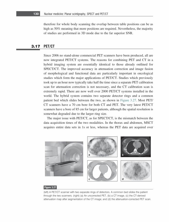
therefore for whole body scanning the overlap between table positions can be ashigh as 50% meaning that more positions are required. Nevertheless, the majorityof studies are performed in 3D mode due to the far superior SNR.
3.17 PET/CT
Since 2006 no stand-alone commercial PET scanners have been produced, all arenow integrated PET/CT systems. The reasons for combining PET and CT in ahybrid imaging system are essentially identical to those already outlined forSPECT/CT. The improved accuracy in attenuation correction and image fusionof morphological and functional data are particularly important in oncologicalstudies which form the major applications of PET/CT. Studies which previouslytook up to an hour now typically take half the time since a separate PET calibrationscan for attenuation correction is not necessary, and the CT calibration scan isextremely rapid. There are now well over 2000 PET/CT systems installed in theworld. The hybrid system contains two separate detector rings and a commonpatient bed which slides between the two, as shown in Figure 3.27. Most PET/CT scanners have a 70 cm bore for both CT and PET. The very latest PET/CTscanners have a bore of 85 cm for larger patients, although the spatial resolution issomewhat degraded due to the larger ring size.
The major issue with PET/CT, as for SPECT/CT, is the mismatch between thedata acquisition times of the two modalities. In the thorax and abdomen, MSCTacquires entire data sets in 1s or less, whereas the PET data are acquired over
a
c d
b
Figure 3.27
(left) A PET/CT scanner with two separate rings of detectors. A common bed slides the patientthrough the two scanners. (right) (a) An uncorrected PET, (b) a CT image, (c) the CT-derivedattenuation map after segmentation of the CT image, and (d) the attenuation-corrected PET scan.
130 Nuclear medicine: Planar scintigraphy, SPECT and PET/CT
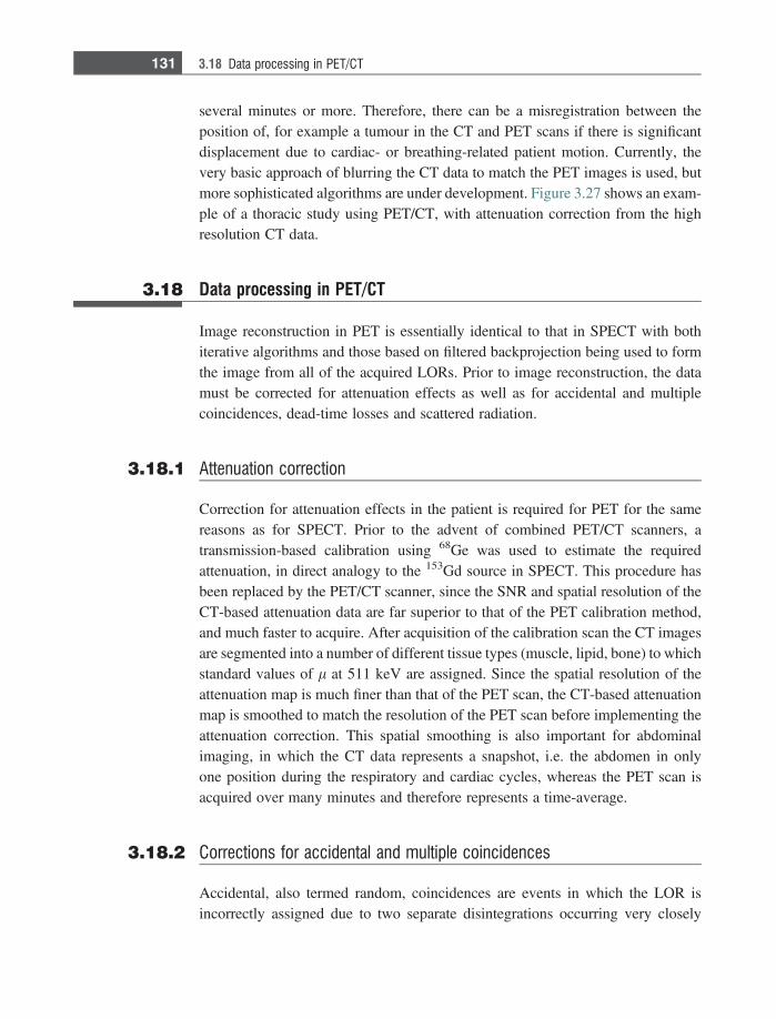
several minutes or more. Therefore, there can be a misregistration between theposition of, for example a tumour in the CT and PET scans if there is significantdisplacement due to cardiac- or breathing-related patient motion. Currently, thevery basic approach of blurring the CT data to match the PET images is used, butmore sophisticated algorithms are under development. Figure 3.27 shows an exam-ple of a thoracic study using PET/CT, with attenuation correction from the highresolution CT data.
3.18 Data processing in PET/CT
Image reconstruction in PET is essentially identical to that in SPECT with bothiterative algorithms and those based on filtered backprojection being used to formthe image from all of the acquired LORs. Prior to image reconstruction, the datamust be corrected for attenuation effects as well as for accidental and multiplecoincidences, dead-time losses and scattered radiation.
3.18.1 Attenuation correction
Correction for attenuation effects in the patient is required for PET for the samereasons as for SPECT. Prior to the advent of combined PET/CT scanners, atransmission-based calibration using 68Ge was used to estimate the requiredattenuation, in direct analogy to the 153Gd source in SPECT. This procedure hasbeen replaced by the PET/CT scanner, since the SNR and spatial resolution of theCT-based attenuation data are far superior to that of the PET calibration method,and much faster to acquire. After acquisition of the calibration scan the CT imagesare segmented into a number of different tissue types (muscle, lipid, bone) to whichstandard values of l at 511 keV are assigned. Since the spatial resolution of theattenuation map is much finer than that of the PET scan, the CT-based attenuationmap is smoothed to match the resolution of the PET scan before implementing theattenuation correction. This spatial smoothing is also important for abdominalimaging, in which the CT data represents a snapshot, i.e. the abdomen in onlyone position during the respiratory and cardiac cycles, whereas the PET scan isacquired over many minutes and therefore represents a time-average.
3.18.2 Corrections for accidental and multiple coincidences
Accidental, also termed random, coincidences are events in which the LOR isincorrectly assigned due to two separate disintegrations occurring very closely
131 3.18 Data processing in PET/CT
in time. In one case, illustrated in Figure 3.28, the first c-rays from each of the twoevents together form an incorrect LOR. A second possibility is that an incorrectLOR is formed due to one c-ray being scattered, also shown in Figure 3.28.Accidental coincidences are uniformly distributed across the imaging field-of-view, and so can cause significant errors in areas which have very low activity.For clinical PET/CT head scanners accidental coincidences constitute ~20% ofthe attributed true coincidences, but for a body scanner the number can be closerto 50%.
The most common method of correcting for random coincidences uses addi-tional parallel timing circuitry, in which a second coincidence timing windowstarts significantly later, typically 60 ns after an event is recorded. The standardcircuit with a 6–12 ns resolving time is used to measure the total number ofcoincidences. The second measurement being delayed well beyond the coinci-dence resolving time means that only accidental coincidences are recorded. Theaccidental coincidences are then subtracted from the acquired data.
An alternative correction method is to measure the number of events recordedby each individual detector. If two detectors i and j are considered, then the rate atwhich accidental coincidences (Cij
acc) are recorded is given by:
Caccij 5 2sRiRj, ð3:18Þ
where Ri and Rj are the single count rates in the individual detectors i and j, and2s is the coincidence resolving time. Therefore, the measured values of Ri and Rj
for each detector pair i and j can be used to estimate the corresponding values ofCij
acc, which are then subtracted from the acquired data. Multiple coincidences can
12
1
Figure 3.28
(left) An accidental coincidence recorded as an LOR between the first c-rays hitting the detector ringfrom radioactive decays at positions 1 and 2 which occur very closely in time. (right) Incorrect LORassigned from a scattered c-ray.
132 Nuclear medicine: Planar scintigraphy, SPECT and PET/CT
also occur, in which more than two events are recorded during the coincidenceresolving time. Estimates for the number of multiple coincidences (Mij) betweentwo detectors can be made using the expression:
Mij � CijsRijNij; ð3:19Þ
where Nij is the total number of detectors operating in coincidence with either ofthe two detectors i and j. Multiple event coincidences are simply discarded beforeimage reconstruction.
3.18.3 Corrections for scattered coincidences
There are two major sources of scattered radiation that contaminate the PET signal,scatter within the body and scatter in the BGO detection crystal itself. BGO has arelatively poor intrinsic energy resolution, and the energy window is typically setto be between 450 and 650 keV for a clinical scan. Since a c-ray that is scattered by45� in the body only loses ~115 keV of its energy, scattered c-rays represent asignificant fraction of the detected c-rays. In 2D PET, scattered c-rays typicallyaccount for only ~10–15% of the detected signal, but in 3D mode up to 50% of thedetected c-rays can be scattered, this larger number due primarily to the elimina-tion of the lead septa. The simplest method of correcting for scatter is to measurethe signal intensity in areas that are outside the patient, and to fit these values to aGaussian shape to estimate the amount of scatter inside the patient. This function isthen subtracted from the raw data to give the corrected image. This approach worksreasonably for relatively homogenous organs such as the brain, but cannot be usedin the abdomen, for example. A second method is to use multiple energy windowmethods, as used in SPECT. The dual-energy window approach typically has thelower window set between 190 and 350 keV, with the upper window at 350–650keV. An alternative method is termed the estimation of trues method (ETM) whichalso uses two windows, but in this case the lower window is 450–650 keV, whichpartially overlaps the upper window between 550 and 650 keV. The ETM makesthe assumption that all of the events in the upper window arise from c-rays thathave not been scattered. These data are then scaled appropriately to equal thenumber of events recorded in the lower window, and these scaled data are thensubtracted from the photopeak energy window. Finally, the most sophisticated butalso most computationally intensive and time-consuming method is an iterativereconstruction based upon simulating the actual scatter using the CT-derivedattenuation maps. The first estimate is simply formed from the data with no scattercorrection: subsequent steps follow the type of iterative data flow already shown inFigure 3.16.
133 3.18 Data processing in PET/CT
3.18.4 Corrections for dead time
As already outlined in Section 3.6.4, there is a maximum count rate that a systemcan record due to finite component response and recovery times. The fractionaldead time of the PET system is defined as the ratio of the measured count rate to thetheoretical count rate if the dead time were zero. The three major sources ofdeadtime in PET scanners are the time taken to integrate the charge from the PMTsafter a scintillation event, the processing of a coincidence event, and the presenceof multiple coincidences in which the data are discarded. Corrections are per-formed based mainly upon a careful characterization of the dead-time associatedwith each component of the PET system, and the number of multiple coincidencesestimated using Equation (3.19).
3.19 Image characteristics
Signal-to-noise
Radiotracer dose, targeting efficiency, image acquisition time, c-ray attenuation inthe patient, system sensitivity and image post-processing play similar roles indetermining the SNR in PET as they do in SPECT scans. As outlined earlier,the intrinsic sensitivity of PET is significantly greater than SPECT due to the lackof collimation requirements and the lower c-ray attenuation in tissue of 511 keVc-rays. In terms of the total number of c-rays emitted by a particular radiotracer,approximately 0.01–0.03% are detected by a SPECT gamma camera, 0.2–0.5% inPET/CT using 2D acquisition-mode, and 2–10% in 3-D PET/CT. Due to thesignificant difference in sensitivity between 2D and 3D, many commercial PET/CT scanners now offer only 3D acquisition.
Contrast-to-noise
In addition to those factors affecting SNR, the CNR is mainly influenced by thecorrection for in Compton-scattered c-rays, and the non-specific uptake of radio-tracer in healthy tissue surrounding the pathology being studied, for example theuptake of FDG in brain, described further in Section 3.21.2.
Spatial resolution
In contrast to SPECT, in which the spatial resolution is significantly worse thedeeper within the body that the radiotracer is located, the in-plane spatial resolutionin PET is much more constant throughout the patient. This is because the inherent‘double detection’ of two c-rays in PET reduces the depth dependence of the PSF.Other factors which influence the spatial resolution of the PET image include:
134 Nuclear medicine: Planar scintigraphy, SPECT and PET/CT
(i) The effective positron range in tissue before it annihilates with an electron:this distance is longer the higher the energy of the emitted positron and theless dense the tissue through which it has to travel. Typical values of themaximum positron energy and corresponding FWHM distances travelled are:18F (640 keV, 0.2 mm), 11C (960 keV, 0.4 mm), 13N (1.2 MeV, 0.6 mm),15O (1.7 MeV, 1 mm), and 82Rb (3.15 MeV, 2.6 mm),
(ii) The non-colinearity of the two c-rays, i.e. the small random deviation from180� of the angle of their relative trajectories. There is a distribution in anglesabout a mean of 180�, with a FHWM of approximately 0.5�. Therefore, thelarger the diameter of the PET detector ring, the greater the effect this has onthe spatial resolution, and
(iii) The dimensions of the detector crystals, with an approximate spatial resolu-tion given by half the detector diameter. Since multiple Compton scatteringinteractions are required to ‘stop’ the c-rays in the crystal there is also anuncertainty in the exact location at which the c-ray first strikes the detector:this uncertainty increases with the thickness of the crystal, as seen previously.
The overall spatial resolution of the system is the combination of all threecomponents:
Rsys �ffiffiffiffiffiffiffiffiffiffiffiffiffiffiffiffiffiffiffiffiffiffiffiffiffiffiffiffiffiffiffiffiffiffiffiffiffiffiffiffiffiffiffiffiffiffiffiR2
detector þ R2range þ R2
1800
q, ð3:20Þ
with typical FWHM values of Rsys of 3–4 mm for a small ring system for brainstudies, and 5–6 mm for a larger whole-body system.
3.20 Time-of-flight PET
The most recent development in commercial PET/CT scanners is that of time-of-flight (TOF) PET [10]. The concept of TOF PET, shown in Figure 3.29, is toconstrain the estimated position of an annihilation to a subsection of the conven-tional LOR between two detectors by measuring the exact times at which the twoc-rays strike the detectors. Ideally, one would be able to constrain the position to apoint, in which case spatial resolution would increase significantly. However, inorder to do this, the timing accuracy of every scintillation event would have to bemuch less than 1 ns, which is not possible. Suppose that one has a timing resolutionof Dt, then the position resolution, Dx, along a line between two detectors isgiven by:
Dx 5cDt2; ð3:21Þ
135 3.20 Time-of-flight PET
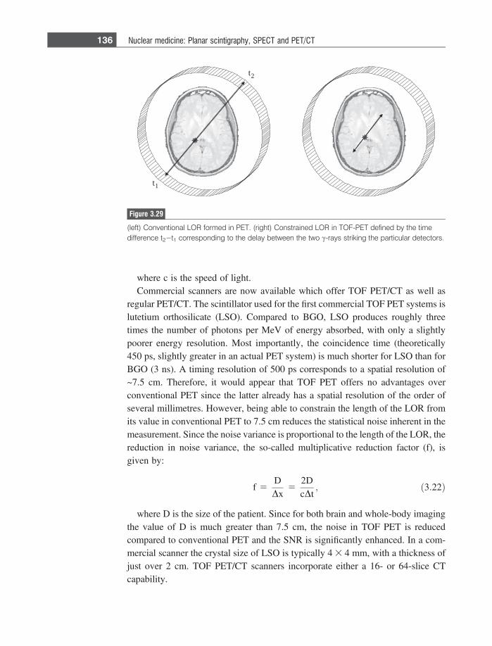
where c is the speed of light.Commercial scanners are now available which offer TOF PET/CT as well as
regular PET/CT. The scintillator used for the first commercial TOF PET systems islutetium orthosilicate (LSO). Compared to BGO, LSO produces roughly threetimes the number of photons per MeV of energy absorbed, with only a slightlypoorer energy resolution. Most importantly, the coincidence time (theoretically450 ps, slightly greater in an actual PET system) is much shorter for LSO than forBGO (3 ns). A timing resolution of 500 ps corresponds to a spatial resolution of~7.5 cm. Therefore, it would appear that TOF PET offers no advantages overconventional PET since the latter already has a spatial resolution of the order ofseveral millimetres. However, being able to constrain the length of the LOR fromits value in conventional PET to 7.5 cm reduces the statistical noise inherent in themeasurement. Since the noise variance is proportional to the length of the LOR, thereduction in noise variance, the so-called multiplicative reduction factor (f), isgiven by:
f 5DDx
52DcDt
; ð3:22Þ
where D is the size of the patient. Since for both brain and whole-body imagingthe value of D is much greater than 7.5 cm, the noise in TOF PET is reducedcompared to conventional PET and the SNR is significantly enhanced. In a com-mercial scanner the crystal size of LSO is typically 4 3 4 mm, with a thickness ofjust over 2 cm. TOF PET/CT scanners incorporate either a 16- or 64-slice CTcapability.
t1
t2
Figure 3.29
(left) Conventional LOR formed in PET. (right) Constrained LOR in TOF-PET defined by the timedifference t22t1 corresponding to the delay between the two c-rays striking the particular detectors.
136 Nuclear medicine: Planar scintigraphy, SPECT and PET/CT
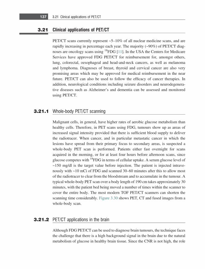
3.21 Clinical applications of PET/CT
PET/CT scans currently represent ~5–10% of all nuclear medicine scans, and arerapidly increasing in percentage each year. The majority (~90%) of PET/CT diag-noses are oncology scans using 18FDG [11]. In the USA the Centers for MedicareServices have approved FDG PET/CT for reimbursement for, amongst others,lung, colorectal, oesophageal and head-and-neck cancers, as well as melanomaand lymphoma. Diagnoses of breast, thyroid and cervical cancer are also verypromising areas which may be approved for medical reimbursement in the nearfuture. PET/CT can also be used to follow the efficacy of cancer therapies. Inaddition, neurological conditions including seizure disorders and neurodegenera-tive diseases such as Alzheimer’s and dementia can be assessed and monitoredusing PET/CT.
3.21.1 Whole-body PET/CT scanning
Malignant cells, in general, have higher rates of aerobic glucose metabolism thanhealthy cells. Therefore, in PET scans using FDG, tumours show up as areas ofincreased signal intensity provided that there is sufficient blood supply to deliverthe radiotracer. When cancer, and in particular metastatic cancer in which thelesions have spread from their primary focus to secondary areas, is suspected awhole-body PET scan is performed. Patients either fast overnight for scansacquired in the morning, or for at least four hours before afternoon scans, sinceglucose competes with 18FDG in terms of cellular uptake. A serum glucose level of~150 mg/dl is the target value before injection. The patient is injected intrave-nously with ~10 mCi of FDG and scanned 30–60 minutes after this to allow mostof the radiotracer to clear from the bloodstream and to accumulate in the tumour. Atypical whole-body PET scan over a body length of 190 cm takes approximately 30minutes, with the patient bed being moved a number of times within the scanner tocover the entire body. The most modern TOF PET/CT scanners can shorten thescanning time considerably. Figure 3.30 shows PET, CT and fused images from awhole-body scan.
3.21.2 PET/CT applications in the brain
Although FDG PET/CT can be used to diagnose brain tumours, the technique facesthe challenge that there is a high background signal in the brain due to the naturalmetabolism of glucose in healthy brain tissue. Since the CNR is not high, the role
137 3.21 Clinical applications of PET/CT
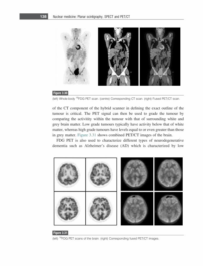
of the CT component of the hybrid scanner in defining the exact outline of thetumour is critical. The PET signal can then be used to grade the tumour bycomparing the activitity within the tumour with that of surrounding white andgrey brain matter. Low grade tumours typically have activity below that of whitematter, whereas high grade tumours have levels equal to or even greater than thosein grey matter. Figure 3.31 shows combined PET/CT images of the brain.
FDG PET is also used to characterize different types of neurodegenerativedementia such as Alzheimer’s disease (AD) which is characterized by low
Figure 3.30
(left) Whole-body 18FDG PET scan. (centre) Corresponding CT scan. (right) Fused PET/CT scan.
Figure 3.31
(left) 18FDG PET scans of the brain. (right) Corresponding fused PET/CT images.
138 Nuclear medicine: Planar scintigraphy, SPECT and PET/CT
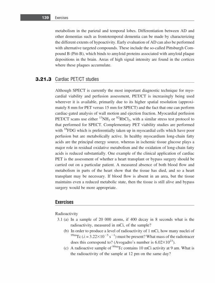
metabolism in the parietal and temporal lobes. Differentiation between AD andother dementias such as frontotemporal dementia can be made by characterizingthe different extents of hypoactivity. Early evaluation of AD can also be performedwith alternative targeted compounds. These include the so-called Pittsburgh Com-pound B (Pitt-B), which binds to amyloid proteins associated with amyloid plaquedepositions in the brain. Areas of high signal intensity are found in the corticeswhere these plaques accumulate.
3.21.3 Cardiac PET/CT studies
Although SPECT is currently the most important diagnostic technique for myo-cardial viability and perfusion assessment, PET/CT is increasingly being usedwherever it is available, primarily due to its higher spatial resolution (approxi-mately 8 mm for PET versus 15 mm for SPECT) and the fact that one can performcardiac-gated analysis of wall motion and ejection fraction. Myocardial perfusionPET/CT scans use either 13NH3 or 82RbCl2, with a similar stress test protocol tothat performed for SPECT. Complementary PET viability studies are performedwith 18FDG which is preferentially taken up in myocardial cells which have poorperfusion but are metabolically active. In healthy myocardium long-chain fattyacids are the principal energy source, whereas in ischemic tissue glucose plays amajor role in residual oxidative metabolism and the oxidation of long-chain fattyacids is reduced substantially. One example of the clinical application of cardiacPET is the assessment of whether a heart transplant or bypass surgery should becarried out on a particular patient. A measured absence of both blood flow andmetabolism in parts of the heart show that the tissue has died, and so a hearttransplant may be necessary. If blood flow is absent in an area, but the tissuemaintains even a reduced metabolic state, then the tissue is still alive and bypasssurgery would be more appropriate.
Exercises
Radioactivity3.1 (a) In a sample of 20 000 atoms, if 400 decay in 8 seconds what is the
radioactivity, measured in mCi, of the sample?(b) In order to produce a level of radioactivity of 1 mCi, how many nuclei of
99mTc (k = 3.2231025 s21) must be present? What mass of the radiotracerdoes this correspond to? (Avogadro’s number is 6.0231023).
(c) A radioactive sample of 99mTc contains 10 mCi activity at 9 am. What isthe radioactivity of the sample at 12 pm on the same day?
139 Exercises

3.2 In a nuclear medicine scan using 99mTc, the image SNR for a 30 minute scanwas 25:1 for an injected radioactive dose of 1 mCi. Imaging began immedi-ately after injection.(a) If the injected dose were tripled to 3 mCi, what would be the image SNR
for a 30 minute scan?(b) If the scan time were doubled to 60 minutes with an initial dose of 1 mCi,
what would be the image SNR?3.3 A dose of 1 mCi of 99mTc is administered to a patient. Calculate the total dose
to the patient if the biological half-life of the radiotracer in the body is:(a) 2 years,(b) 6 hours,(c) 2 minutes.
The technetium generator.3.4 In the technetium generator, show mathematically that if k2� k1, the radio-
activities of the parent and daughter nuclei become equal in value at longtimes.
3.5 Using the equations derived in the analysis of the technetium generator,plot graphs of the activity of parent and daughter nuclei for the followingcases:(a) s1/2 (parent) = 600 hours, s1/2 (daughter) = 6 hours,(b) s1/2 (parent) = 6.1 hours, s1/2 (daughter) = 6 hours,(c) s1/2 (parent) = 0.6 hours, s1/2 (daughter) = 6 hours.
3.6 Calculate the exact time at which the first three ‘milkings’ of the technetiumcow should be performed.
3.7 Do the tops of the curves in Figure 3.4 lie at the same values that would havebeen obtained if the technetium cow were not milked at all?
3.8 Rather than waiting 24 hours, only 6 hours are left between milkings. Plot thegraph of radioactivity over the first two days.
The gamma camera.3.9 Calculate the magnification factor for the pinhole collimator shown in Figure
3.32(a). What implications does this have for image distortions?3.10 If the acceptance window for a planar nuclear medicine scan is set to 15%,
what is the maximum angle that a c-ray could be Compton scattered and stillbe accepted if it strikes the scintillation crystal?
3.11 What is the energy of a c-ray which has been Compton scattered at an angleof 30� in the body?
3.12 (i) The thickness of the lead septa is chosen to ensure that only 5% of thec-rays penetrate from one collimator hole to the adjacent one. UsingFigure 3.32(b) show that the thickness is given by [6d/l]/[L23/l].
140 Nuclear medicine: Planar scintigraphy, SPECT and PET/CT
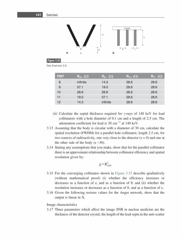
(ii) Calculate the septal thickness required for c-rays of 140 keV for leadcollimators with a hole diameter of 0.1 cm and a length of 2.5 cm. Theattenuation coefficient for lead is 30 cm21 at 140 keV.
3.13 Assuming that the body is circular with a diameter of 30 cm, calculate thespatial resolution (FWHM) for a parallel hole collimator, length 2.5 cm, fortwo sources of radioactivity, one very close to the detector (z = 0) and one atthe other side of the body (z ~30).
3.14 Stating any assumptions that you make, show that for the parallel collimatorthere is an approximate relationship between collimator efficiency and spatialresolution given by:
g } R2coll:
3.15 For the converging collimator shown in Figure 3.33 describe qualitatively(without mathematical proof) (i) whether the efficiency increases ordecreases as a function of z, and as a function of h, and (ii) whether theresolution increases or decreases as a function of h, and as a function of z.
3.16 Given the following resistor values for the Anger network, show that theoutput is linear in X.
Image characteristics3.17 Three parameters which affect the image SNR in nuclear medicine are the
thickness of the detector crystal, the length of the lead septa in the anti-scatter
crystal
L
td
L
d z
ba
Figure 3.32
See Exercise 3.9.
PMT RX+ (X) RX2 (X) RY+ (X) RY2 (X)
8 infinite 14.3 28.6 28.6
9 57.1 19.0 28.6 28.6
10 28.6 28.6 28.6 28.6
11 19.0 57.1 28.6 28.6
12 14.3 infinite 28.6 28.6
141 Exercises
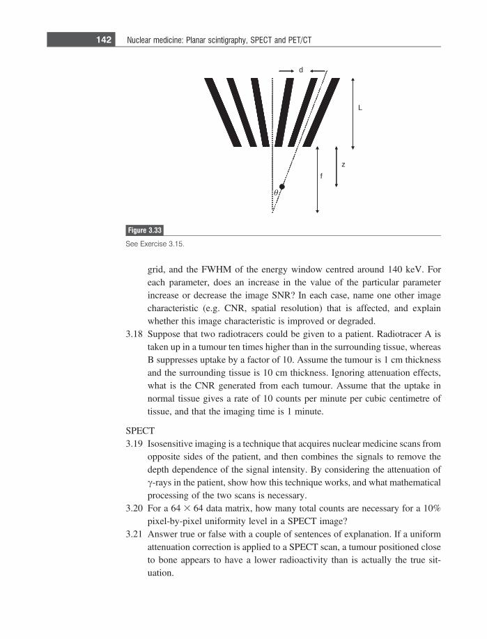
grid, and the FWHM of the energy window centred around 140 keV. Foreach parameter, does an increase in the value of the particular parameterincrease or decrease the image SNR? In each case, name one other imagecharacteristic (e.g. CNR, spatial resolution) that is affected, and explainwhether this image characteristic is improved or degraded.
3.18 Suppose that two radiotracers could be given to a patient. Radiotracer A istaken up in a tumour ten times higher than in the surrounding tissue, whereasB suppresses uptake by a factor of 10. Assume the tumour is 1 cm thicknessand the surrounding tissue is 10 cm thickness. Ignoring attenuation effects,what is the CNR generated from each tumour. Assume that the uptake innormal tissue gives a rate of 10 counts per minute per cubic centimetre oftissue, and that the imaging time is 1 minute.
SPECT3.19 Isosensitive imaging is a technique that acquires nuclear medicine scans from
opposite sides of the patient, and then combines the signals to remove thedepth dependence of the signal intensity. By considering the attenuation ofc-rays in the patient, show how this technique works, and what mathematicalprocessing of the two scans is necessary.
3.20 For a 64 3 64 data matrix, how many total counts are necessary for a 10%pixel-by-pixel uniformity level in a SPECT image?
3.21 Answer true or false with a couple of sentences of explanation. If a uniformattenuation correction is applied to a SPECT scan, a tumour positioned closeto bone appears to have a lower radioactivity than is actually the true sit-uation.
d
L
zf
θ
Figure 3.33
See Exercise 3.15.
142 Nuclear medicine: Planar scintigraphy, SPECT and PET/CT
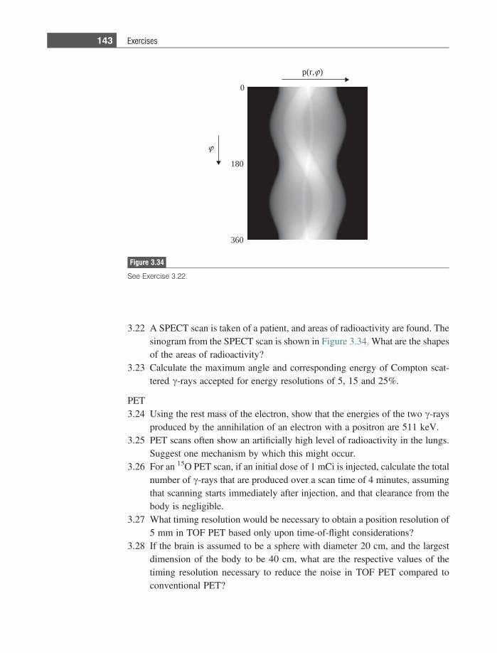
3.22 A SPECT scan is taken of a patient, and areas of radioactivity are found. Thesinogram from the SPECT scan is shown in Figure 3.34. What are the shapesof the areas of radioactivity?
3.23 Calculate the maximum angle and corresponding energy of Compton scat-tered c-rays accepted for energy resolutions of 5, 15 and 25%.
PET3.24 Using the rest mass of the electron, show that the energies of the two c-rays
produced by the annihilation of an electron with a positron are 511 keV.3.25 PET scans often show an artificially high level of radioactivity in the lungs.
Suggest one mechanism by which this might occur.3.26 For an 15O PET scan, if an initial dose of 1 mCi is injected, calculate the total
number of c-rays that are produced over a scan time of 4 minutes, assumingthat scanning starts immediately after injection, and that clearance from thebody is negligible.
3.27 What timing resolution would be necessary to obtain a position resolution of5 mm in TOF PET based only upon time-of-flight considerations?
3.28 If the brain is assumed to be a sphere with diameter 20 cm, and the largestdimension of the body to be 40 cm, what are the respective values of thetiming resolution necessary to reduce the noise in TOF PET compared toconventional PET?
180
0
360
p(r, )
Figure 3.34
See Exercise 3.22.
143 Exercises
3.29 Suggest why a PET/CT scanner operating in 2D mode has a relatively uni-form axial sensitivity profile, whereas in 3D mode the sensitivity is muchhigher at the centre of the scanner.
3.30 Suggest why a curvilinear region of low signal intensity is often seen onPET/CT scans of the thorax and abdomen, which parallels the dome of thediaphragm.
References
[1] Anger H. Scintillation camera. Review of Scientific Instruments 1958;29,27–33.[2] O’Connor MK and Kemp BJ. Single-photon emission computed tomography/
Computed tomography: Basic instrumentation and innovations. Seminars in Nuclear
Medicine 2006:36, 258–66.[3] Seo Y, Mari C and Hasegawa BH. Technological development and advances in
single-photon emission computed tomography/computed tomography. Seminars in
Nuclear Medicine 2008:38, 177–198.[4] Robertson JS, Marr RB, Rosenblum M, Radeka V and Yamamoto YL. Thirty-two-
crystal positron transverse section detector. In: Freedmen GS, editor. Tomographic
imaging in nuclear medicine. New York: Society of Nuclear Medicine; 1973:142–53.
[5] Ter-Pogossian MM, Mullani NA, Hood J, Higgins CS and Curie M. A multi-slicepostitron emission computed tomograph (PETT IV) yielding transverse andlongitudinal images. Radiology 1978:128, 477–484.
[6] Rahmin A and Zaidi H. PET vs. SPECT: strengths, limitations and challenges.Nuclear Medicine Communications 2008:29, 193–207.
[7] Mittra E and Quon A. Positron emission tomography/computed tomography: thecurrent technology and applications. Radiological Clinics of North America 2009:47,147–60.
[8] Gallagher GM, Ansari A, Atkins H et al. Radiopharmaceuticals XXVII. 18F-labeled2-deoxy-2-fluoro-D-glucose as a radiopharmaceutical for measuring regionalmyocardial glucose metabolism in vivo: tissue distribution and imaging studies inanimals. Journal of Nuclear Medicine 1977: 18, 990–6.
[9] van Eijk CWE. Radiation detector developments in medical applications: inorganicscintillators in positron emission tomography. Radiation Protection Dosimetry
2008:129, 13–21.[10] Moses WM. Recent advances and future advances in time-of-flight PET. Nuclear
Instrument Methods Physics Research A 2007:580, 919–24.[11] Pan T and Mawlawi O. PET/CT in radiation oncology. Medical Physics 2008:35,
4955–66.
144 Nuclear medicine: Planar scintigraphy, SPECT and PET/CT
4 Ultrasound imaging
4.1 Introduction
Of all the standard clinical imaging techniques ultrasound is by far the leastexpensive and most portable (including handheld units smaller than a laptopcomputer), and can acquire continuous images at a real-time frame rate with fewor no safety concerns. In addition to morphological and structural information,ultrasound can also measure blood flow in real-time, and produce detailed maps ofblood velocity within a given vessel. Ultrasound finds very wide use in obstetricsand gynaecology, due to the lack of ionizing radiation or strong magnetic fields.The real-time nature of the imaging is also important in measuring parameters suchas foetal heart function. Ultrasound is used in many cardiovascular applications,being able to detect mitral valve and septal insufficiencies. General imaging appli-cations include liver cysts, aortic aneurysms, and obstructive atherosclerosis in thecarotids. Ultrasound imaging is also used very often to guide the path and position-ing of a needle in tissue biopsies.
Ultrasound is a mechanical wave, with a frequency for clinical use between 1and 15 MHz. The speed of sound in tissue is ~1540 m/s, and so the range ofwavelengths of ultrasound in tissue is between ~0.1 and 1.5 mm. The ultrasoundwaves are produced by a transducer, as shown in Figure 4.1, which typically has anarray of up to 512 individual active sources. In the simplest image acquisitionscheme, small subgroups of these elements are fired sequentially to produce paral-lel ultrasound beams. As the ultrasound passes through tissue, a small fraction ofthe energy is reflected from the boundaries between tissues which have slightlydifferent acoustic and physical properties: the remaining energy of the beam istransmitted through the boundary. The reflected waves are detected by the trans-ducer and the distance to each tissue boundary is calculated from the time betweenpulse transmission and signal reception: thus ultrasound imaging is very similarto techniques such as radar. As soon as the signal from the deepest tissueboundary has been detected from one beam, the next adjacent beam of ultrasoundis emitted, and this process is repeated until the entire image has been acquired.Due to the relatively high speed of ultrasound through tissue, entire images can be
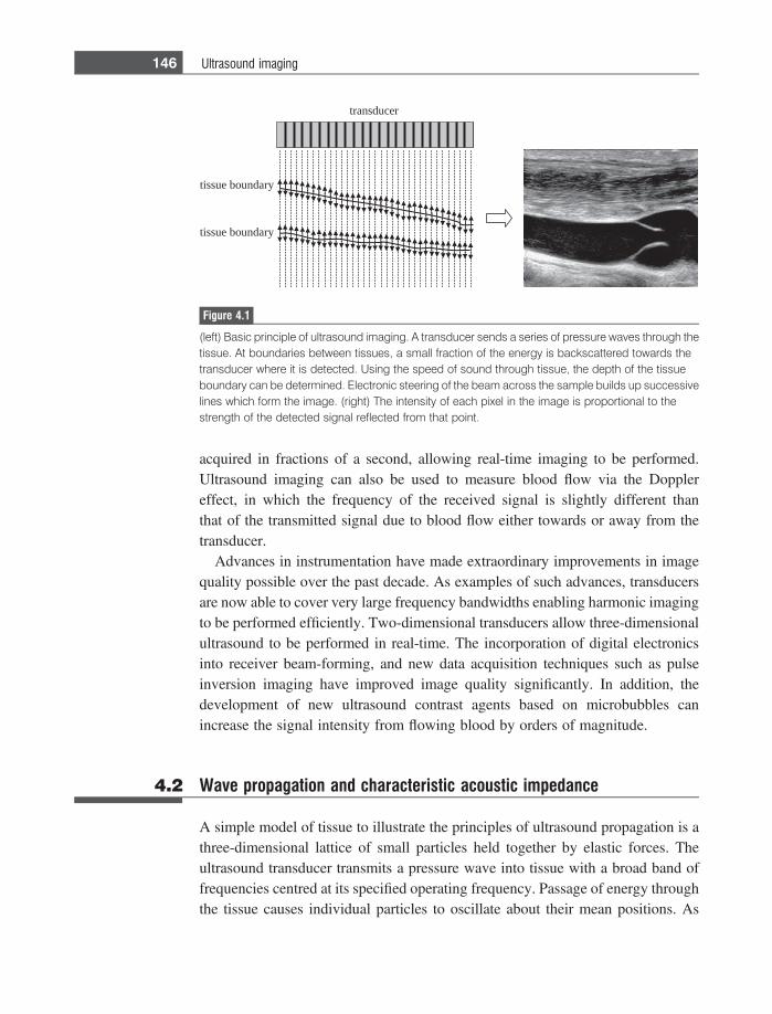
acquired in fractions of a second, allowing real-time imaging to be performed.Ultrasound imaging can also be used to measure blood flow via the Dopplereffect, in which the frequency of the received signal is slightly different thanthat of the transmitted signal due to blood flow either towards or away from thetransducer.
Advances in instrumentation have made extraordinary improvements in imagequality possible over the past decade. As examples of such advances, transducersare now able to cover very large frequency bandwidths enabling harmonic imagingto be performed efficiently. Two-dimensional transducers allow three-dimensionalultrasound to be performed in real-time. The incorporation of digital electronicsinto receiver beam-forming, and new data acquisition techniques such as pulseinversion imaging have improved image quality significantly. In addition, thedevelopment of new ultrasound contrast agents based on microbubbles canincrease the signal intensity from flowing blood by orders of magnitude.
4.2 Wave propagation and characteristic acoustic impedance
A simple model of tissue to illustrate the principles of ultrasound propagation is athree-dimensional lattice of small particles held together by elastic forces. Theultrasound transducer transmits a pressure wave into tissue with a broad band offrequencies centred at its specified operating frequency. Passage of energy throughthe tissue causes individual particles to oscillate about their mean positions. As
tissue boundary
tissue boundary
transducer
Figure 4.1
(left) Basic principle of ultrasound imaging. A transducer sends a series of pressure waves through thetissue. At boundaries between tissues, a small fraction of the energy is backscattered towards thetransducer where it is detected. Using the speed of sound through tissue, the depth of the tissueboundary can be determined. Electronic steering of the beam across the sample builds up successivelines which form the image. (right) The intensity of each pixel in the image is proportional to thestrength of the detected signal reflected from that point.
146 Ultrasound imaging
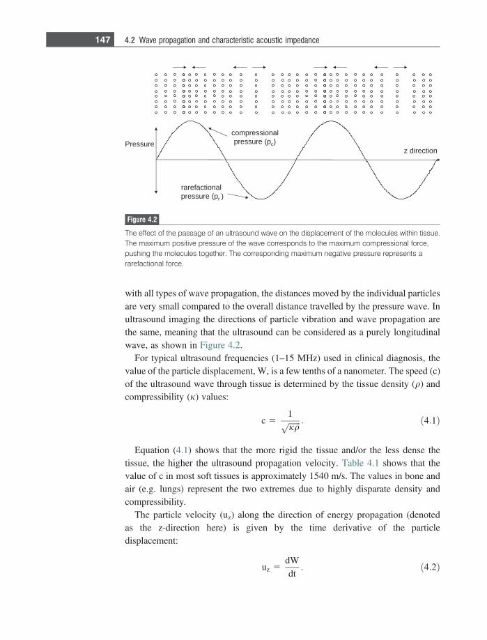
with all types of wave propagation, the distances moved by the individual particlesare very small compared to the overall distance travelled by the pressure wave. Inultrasound imaging the directions of particle vibration and wave propagation arethe same, meaning that the ultrasound can be considered as a purely longitudinalwave, as shown in Figure 4.2.
For typical ultrasound frequencies (1–15 MHz) used in clinical diagnosis, thevalue of the particle displacement, W, is a few tenths of a nanometer. The speed (c)of the ultrasound wave through tissue is determined by the tissue density (q) andcompressibility (j) values:
c 51ffiffiffiffiffiffijqp : ð4:1Þ
Equation (4.1) shows that the more rigid the tissue and/or the less dense thetissue, the higher the ultrasound propagation velocity. Table 4.1 shows that thevalue of c in most soft tissues is approximately 1540 m/s. The values in bone andair (e.g. lungs) represent the two extremes due to highly disparate density andcompressibility.
The particle velocity (uz) along the direction of energy propagation (denotedas the z-direction here) is given by the time derivative of the particledisplacement:
uz 5dWdt: ð4:2Þ
z directionPressure
compressionalpressure (pc)
rarefactionalpressure (pr )
Figure 4.2
The effect of the passage of an ultrasound wave on the displacement of the molecules within tissue.The maximum positive pressure of the wave corresponds to the maximum compressional force,pushing the molecules together. The corresponding maximum negative pressure represents ararefactional force.
147 4.2 Wave propagation and characteristic acoustic impedance
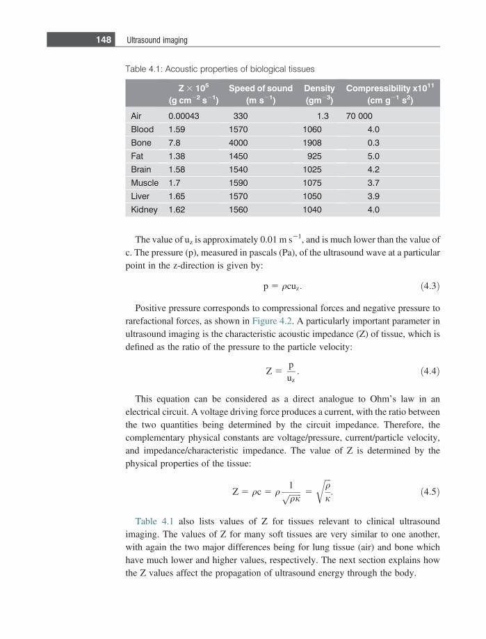
The value of uz is approximately 0.01 m s21, and is much lower than the value ofc. The pressure (p), measured in pascals (Pa), of the ultrasound wave at a particularpoint in the z-direction is given by:
p 5 qcuz: ð4:3Þ
Positive pressure corresponds to compressional forces and negative pressure torarefactional forces, as shown in Figure 4.2. A particularly important parameter inultrasound imaging is the characteristic acoustic impedance (Z) of tissue, which isdefined as the ratio of the pressure to the particle velocity:
Z 5puz: ð4:4Þ
This equation can be considered as a direct analogue to Ohm’s law in anelectrical circuit. A voltage driving force produces a current, with the ratio betweenthe two quantities being determined by the circuit impedance. Therefore, thecomplementary physical constants are voltage/pressure, current/particle velocity,and impedance/characteristic impedance. The value of Z is determined by thephysical properties of the tissue:
Z 5 qc 5 q1ffiffiffiffiffiffiqjp 5
ffiffiffiqj
r: ð4:5Þ
Table 4.1 also lists values of Z for tissues relevant to clinical ultrasoundimaging. The values of Z for many soft tissues are very similar to one another,with again the two major differences being for lung tissue (air) and bone whichhave much lower and higher values, respectively. The next section explains howthe Z values affect the propagation of ultrasound energy through the body.
Table 4.1: Acoustic properties of biological tissues
Z 3 105
(g cm22 s21)Speed of sound
(m s21)Density(gm23)
Compressibility x1011
(cm g21 s2)
Air 0.00043 330 1.3 70 000
Blood 1.59 1570 1060 4.0
Bone 7.8 4000 1908 0.3
Fat 1.38 1450 925 5.0
Brain 1.58 1540 1025 4.2
Muscle 1.7 1590 1075 3.7
Liver 1.65 1570 1050 3.9
Kidney 1.62 1560 1040 4.0
148 Ultrasound imaging
Example 4.1 Given the values of c = 1540 m s21 and q = 1.05 g cm23 for brain tissue, calculatethe values of the characteristic acoustic impedance and compressibility.
Solution The characteristic impedance of brain tissue is given by:
Z 5 qc 5 1:05ðg cm�3Þ 3 154000ðcm s�1Þ 5 1:58 3 105g cm�2s�1:
From Equation (4.5), Z2 = q/j and so:
j 5 q=Z25 1:05ðg cm�3Þ=ð1:58 3 105Þ2g2 cm�4s�2
5 4:2 3 10�11 cm g�1s2:
Using the SI definition of 1 Pascal (Pa) as 1 kg m21 s22, which is equivalent to10 g cm21 s22, the units of compressibility are the same as inverse pressure.
4.3 Wave reflection, refraction and scattering in tissue
As the ultrasound beam passes through tissue it encounters different tissues withdifferent acoustic properties, as shown in Table 4.1. Whenever either a boundarybetween two tissues, or small structures within a homogeneous tissue, are encoun-tered the differences in acoustic properties result in a fraction of the energy of theultrasound beam being backscattered towards the transducer, where it forms thedetected signal.
4.3.1 Reflection, transmission and refraction at tissue boundaries
When an ultrasound wave encounters a boundary between two tissues with differ-ent values of Z, a certain fraction of the wave energy is backscattered (or reflected)towards the transducer, with the remainder being transmitted through the boundarydeeper into the body. In the first case considered here, the boundary is shown inFigure 4.3 as being flat, implying that its dimensions are much greater than theultrasound wavelength, for example� 1 mm for a 1.5 MHz central frequency. Inthe general situation shown in Figure 4.3, the incident ultrasound wave strikes theboundary at an angle hi.
The following equations relate the angles of incidence (hi) and reflection (hr),angles of incidence (hi) and transmission (ht), reflected (pr) and transmitted (pt)pressures, and reflected (Ir) and transmitted (It) intensities:
149 4.3 Wave reflection, refraction and scattering in tissue
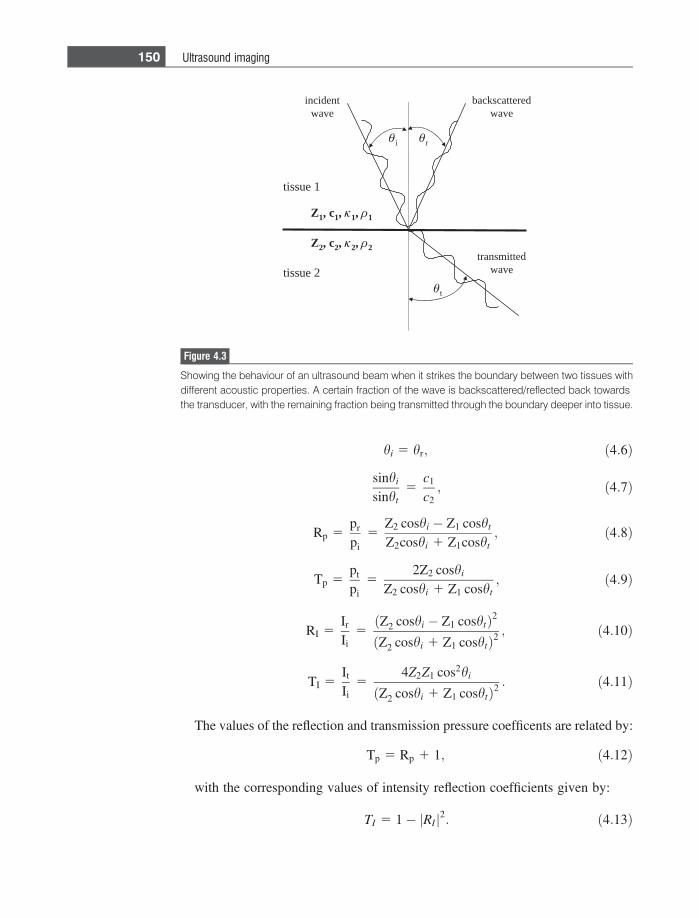
hi 5 hr; ð4:6Þ
sinhi
sinht5
c1
c2; ð4:7Þ
Rp 5pr
pi5
Z2 coshi � Z1 cosht
Z2coshi 1 Z1cosht; ð4:8Þ
Tp 5pt
pi5
2Z2 coshi
Z2 coshi 1 Z1 cosht; ð4:9Þ
RI 5Ir
Ii5ðZ2 coshi � Z1 coshtÞ2
ðZ2 coshi 1 Z1 coshtÞ2; ð4:10Þ
TI 5It
Ii5
4Z2Z1 cos2hi
ðZ2 coshi 1 Z1 coshtÞ2: ð4:11Þ
The values of the reflection and transmission pressure coefficents are related by:
Tp 5 Rp 1 1; ð4:12Þ
with the corresponding values of intensity reflection coefficients given by:
TI 5 1� RIj j2: ð4:13Þ
transmittedwave
backscatteredwave
incidentwave
Z1, c1, 1, 1
i r
t
Z2, c2, 2, 2
tissue 1
tissue 2
Figure 4.3
Showing the behaviour of an ultrasound beam when it strikes the boundary between two tissues withdifferent acoustic properties. A certain fraction of the wave is backscattered/reflected back towardsthe transducer, with the remaining fraction being transmitted through the boundary deeper into tissue.
150 Ultrasound imaging
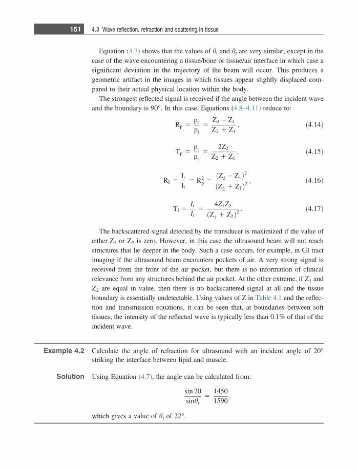
Equation (4.7) shows that the values of hi and ht are very similar, except in thecase of the wave encountering a tissue/bone or tissue/air interface in which case asignificant deviation in the trajectory of the beam will occur. This produces ageometric artifact in the images in which tissues appear slightly displaced com-pared to their actual physical location within the body.
The strongest reflected signal is received if the angle between the incident waveand the boundary is 90�. In this case, Equations (4.8–4.11) reduce to:
Rp 5pr
pi5
Z2 � Z1
Z2 1 Z1; ð4:14Þ
Tp 5pt
pi5
2Z2
Z2 1 Z1; ð4:15Þ
RI 5Ir
Ii5 R2
p 5ðZ2 � Z1Þ2
ðZ2 1 Z1Þ2; ð4:16Þ
TI 5It
Ii5
4Z1Z2
ðZ1 1 Z2Þ2: ð4:17Þ
The backscattered signal detected by the transducer is maximized if the value ofeither Z1 or Z2 is zero. However, in this case the ultrasound beam will not reachstructures that lie deeper in the body. Such a case occurs, for example, in GI tractimaging if the ultrasound beam encounters pockets of air. A very strong signal isreceived from the front of the air pocket, but there is no information of clinicalrelevance from any structures behind the air pocket. At the other extreme, if Z1 andZ2 are equal in value, then there is no backscattered signal at all and the tissueboundary is essentially undetectable. Using values of Z in Table 4.1 and the reflec-tion and transmission equations, it can be seen that, at boundaries between softtissues, the intensity of the reflected wave is typically less than 0.1% of that of theincident wave.
Example 4.2 Calculate the angle of refraction for ultrasound with an incident angle of 20�striking the interface between lipid and muscle.
Solution Using Equation (4.7), the angle can be calculated from:
sin 20sinht
514501590
;
which gives a value of ht of 22�.
151 4.3 Wave reflection, refraction and scattering in tissue
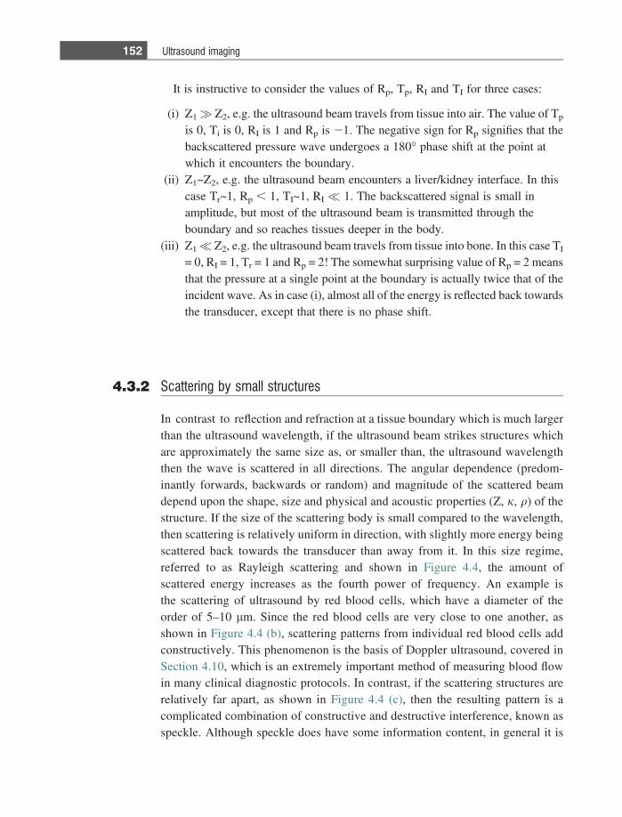
It is instructive to consider the values of Rp, Tp, RI and TI for three cases:
(i) Z1� Z2, e.g. the ultrasound beam travels from tissue into air. The value of Tp
is 0, Ti is 0, RI is 1 and Rp is 21. The negative sign for Rp signifies that thebackscattered pressure wave undergoes a 180� phase shift at the point atwhich it encounters the boundary.
(ii) Z1~Z2, e.g. the ultrasound beam encounters a liver/kidney interface. In thiscase Tr~1, Rp , 1, TI~1, RI � 1. The backscattered signal is small inamplitude, but most of the ultrasound beam is transmitted through theboundary and so reaches tissues deeper in the body.
(iii) Z1� Z2, e.g. the ultrasound beam travels from tissue into bone. In this case TI
= 0, RI = 1, Tr = 1 and Rp = 2! The somewhat surprising value of Rp = 2 meansthat the pressure at a single point at the boundary is actually twice that of theincident wave. As in case (i), almost all of the energy is reflected back towardsthe transducer, except that there is no phase shift.
4.3.2 Scattering by small structures
In contrast to reflection and refraction at a tissue boundary which is much largerthan the ultrasound wavelength, if the ultrasound beam strikes structures whichare approximately the same size as, or smaller than, the ultrasound wavelengththen the wave is scattered in all directions. The angular dependence (predom-inantly forwards, backwards or random) and magnitude of the scattered beamdepend upon the shape, size and physical and acoustic properties (Z, j, q) of thestructure. If the size of the scattering body is small compared to the wavelength,then scattering is relatively uniform in direction, with slightly more energy beingscattered back towards the transducer than away from it. In this size regime,referred to as Rayleigh scattering and shown in Figure 4.4, the amount ofscattered energy increases as the fourth power of frequency. An example isthe scattering of ultrasound by red blood cells, which have a diameter of theorder of 5–10 lm. Since the red blood cells are very close to one another, asshown in Figure 4.4 (b), scattering patterns from individual red blood cells addconstructively. This phenomenon is the basis of Doppler ultrasound, covered inSection 4.10, which is an extremely important method of measuring blood flowin many clinical diagnostic protocols. In contrast, if the scattering structures arerelatively far apart, as shown in Figure 4.4 (c), then the resulting pattern is acomplicated combination of constructive and destructive interference, known asspeckle. Although speckle does have some information content, in general it is
152 Ultrasound imaging
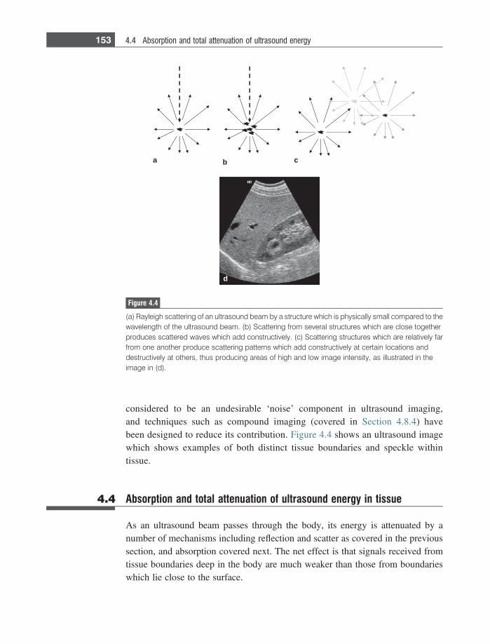
considered to be an undesirable ‘noise’ component in ultrasound imaging,and techniques such as compound imaging (covered in Section 4.8.4) havebeen designed to reduce its contribution. Figure 4.4 shows an ultrasound imagewhich shows examples of both distinct tissue boundaries and speckle withintissue.
4.4 Absorption and total attenuation of ultrasound energy in tissue
As an ultrasound beam passes through the body, its energy is attenuated by anumber of mechanisms including reflection and scatter as covered in the previoussection, and absorption covered next. The net effect is that signals received fromtissue boundaries deep in the body are much weaker than those from boundarieswhich lie close to the surface.
a b c
d
Figure 4.4
(a) Rayleigh scattering of an ultrasound beam by a structure which is physically small compared to thewavelength of the ultrasound beam. (b) Scattering from several structures which are close togetherproduces scattered waves which add constructively. (c) Scattering structures which are relatively farfrom one another produce scattering patterns which add constructively at certain locations anddestructively at others, thus producing areas of high and low image intensity, as illustrated in theimage in (d).
153 4.4 Absorption and total attenuation of ultrasound energy
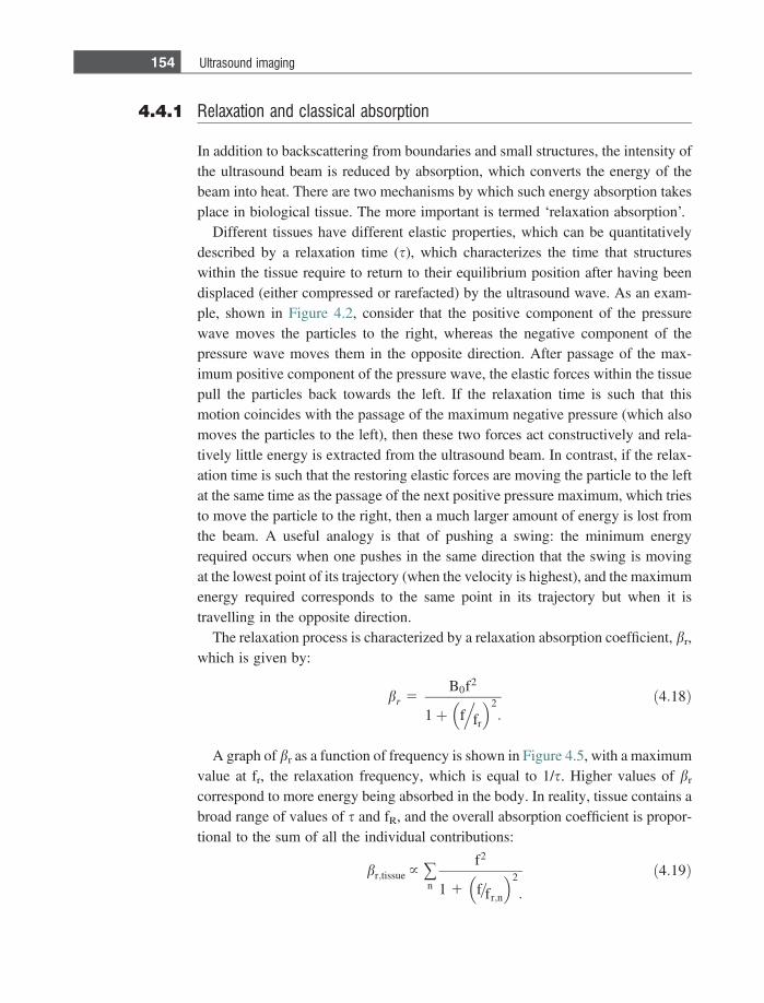
4.4.1 Relaxation and classical absorption
In addition to backscattering from boundaries and small structures, the intensity ofthe ultrasound beam is reduced by absorption, which converts the energy of thebeam into heat. There are two mechanisms by which such energy absorption takesplace in biological tissue. The more important is termed ‘relaxation absorption’.
Different tissues have different elastic properties, which can be quantitativelydescribed by a relaxation time (s), which characterizes the time that structureswithin the tissue require to return to their equilibrium position after having beendisplaced (either compressed or rarefacted) by the ultrasound wave. As an exam-ple, shown in Figure 4.2, consider that the positive component of the pressurewave moves the particles to the right, whereas the negative component of thepressure wave moves them in the opposite direction. After passage of the max-imum positive component of the pressure wave, the elastic forces within the tissuepull the particles back towards the left. If the relaxation time is such that thismotion coincides with the passage of the maximum negative pressure (which alsomoves the particles to the left), then these two forces act constructively and rela-tively little energy is extracted from the ultrasound beam. In contrast, if the relax-ation time is such that the restoring elastic forces are moving the particle to the leftat the same time as the passage of the next positive pressure maximum, which triesto move the particle to the right, then a much larger amount of energy is lost fromthe beam. A useful analogy is that of pushing a swing: the minimum energyrequired occurs when one pushes in the same direction that the swing is movingat the lowest point of its trajectory (when the velocity is highest), and the maximumenergy required corresponds to the same point in its trajectory but when it istravelling in the opposite direction.
The relaxation process is characterized by a relaxation absorption coefficient, br,which is given by:
br 5B0f2
1þ�
f fr
. �2:
ð4:18Þ
A graph of br as a function of frequency is shown in Figure 4.5, with a maximumvalue at fr, the relaxation frequency, which is equal to 1/s. Higher values of br
correspond to more energy being absorbed in the body. In reality, tissue contains abroad range of values of s and fR, and the overall absorption coefficient is propor-tional to the sum of all the individual contributions:
br;tissue } +n
f2
1 1�
f=fr;n
�2
:
ð4:19Þ
154 Ultrasound imaging
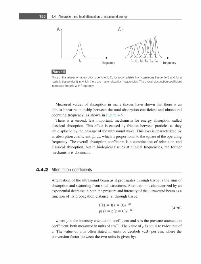
Measured values of absorption in many tissues have shown that there is analmost linear relationship between the total absorption coefficient and ultrasoundoperating frequency, as shown in Figure 4.5.
There is a second, less important, mechanism for energy absorption calledclassical absorption. This effect is caused by friction between particles as theyare displaced by the passage of the ultrasound wave. This loss is characterized byan absorption coefficient, bclass, which is proportional to the square of the operatingfrequency. The overall absorption coefficient is a combination of relaxation andclassical absorption, but in biological tissues at clinical frequencies, the formermechanism is dominant.
4.4.2 Attenuation coefficients
Attenuation of the ultrasound beam as it propagates through tissue is the sum ofabsorption and scattering from small structures. Attenuation is characterized by anexponential decrease in both the pressure and intensity of the ultrasound beam as afunction of its propagation distance, z, through tissue:
I zð Þ 5 I z 5 0ð Þe�lz
pðzÞ 5 p z 5 0ð Þe�az ; ð4:20Þ
where l is the intensity attenuation coefficient and a is the pressure attenuationcoefficient, both measured in units of cm21. The value of l is equal to twice that ofa. The value of l is often stated in units of decibels (dB) per cm, where theconversion factor between the two units is given by:
frequencyfr1
r
fr2 fr3 fr4 fr5 fr6frequency
r
fr
Figure 4.5
Plots of the relaxation absorption coefficient, br, for a completely homogeneous tissue (left) and for arealistic tissue (right) in which there are many relaxation frequencies. The overall absorption coefficientincreases linearly with frequency.
155 4.4 Absorption and total attenuation of ultrasound energy
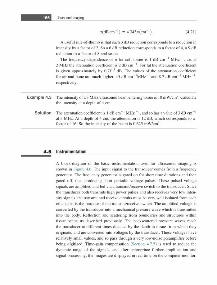
l dB cm�1� �
5 4:343l cm�1� �
: ð4:21Þ
A useful rule-of-thumb is that each 3 dB reduction corresponds to a reduction inintensity by a factor of 2. So a 6 dB reduction corresponds to a factor of 4, a 9 dBreduction to a factor of 8 and so on.
The frequency dependence of l for soft tissue is 1 dB cm21 MHz21, i.e. at2 MHz the attenuation coefficient is 2 dB cm21. For fat the attenuation coefficientis given approximately by 0.7f1.5 dB. The values of the attenuation coefficientfor air and bone are much higher, 45 dB cm21MHz21 and 8.7 dB cm21 MHz21,respectively.
Example 4.3 The intensity of a 3 MHz ultrasound beam entering tissue is 10 mW/cm2. Calculatethe intensity at a depth of 4 cm.
Solution The attenuation coefficient is 1 dB cm21 MHz 21, and so has a value of 3 dB cm21
at 3 MHz. At a depth of 4 cm, the attenuation is 12 dB, which corresponds to afactor of 16. So the intensity of the beam is 0.625 mW/cm2.
4.5 Instrumentation
A block-diagram of the basic instrumentation used for ultrasound imaging isshown in Figure 4.6. The input signal to the transducer comes from a frequencygenerator. The frequency generator is gated on for short time durations and thengated off, thus producing short periodic voltage pulses. These pulsed voltagesignals are amplified and fed via a transmit/receive switch to the transducer. Sincethe transducer both transmits high power pulses and also receives very low inten-sity signals, the transmit and receive circuits must be very well isolated from eachother; this is the purpose of the transmit/receive switch. The amplified voltage isconverted by the transducer into a mechanical pressure wave which is transmittedinto the body. Reflection and scattering from boundaries and structures withintissue occur, as described previously. The backscattered pressure waves reachthe transducer at different times dictated by the depth in tissue from which theyoriginate, and are converted into voltages by the transducer. These voltages haverelatively small values, and so pass through a very low-noise preamplifier beforebeing digitized. Time-gain compensation (Section 4.7.5) is used to reduce thedynamic range of the signals, and after appropriate further amplification andsignal processing, the images are displayed in real time on the computer monitor.
156 Ultrasound imaging
Additional circuitry in both the transmit and receive channels is requiredwhen using phased array transducers, and this is covered in Sections 4.7.3 and4.7.4.
4.6 Single element ultrasound transducers
Although the vast majority of transducers consist of a large array of small elements,it is useful to consider first the properties of a single element transducer, shownschematically in Figure 4.7. Shaped piezoelectric material is the active element ofall ultrasound transducers, and is formed from a composite of lead zirconatetitanate (PZT). Fine powders of the three metal oxides are mixed and then heatedto high temperatures ( . 120 �C) and placed in a strong electric field, with a valueof tens of kV per cm. This field aligns the dipoles within the material, and confersthe property of being piezoelectric, i.e. able to convert an oscillating voltage tochanges in physical dimension, and vice versa. Thin rods of PZT are embedded ina resin, and the material is then formed into the required shape and size. In the caseof a single element transducer, the element is usually disk-shaped or formed into aspherical or cylindrical shell. The two faces of the element are coated with a thinlayer of silver and connected via bonding wires to a coaxial cable leading to the
Tx/Rxswitch
Time-gaincompensation
logarithmiccompression
Analogue-to-digitalconverter
Real-timedisplay
transducer
Figure 4.6
The major elements of a basic ultrasound imaging system.
157 4.6 Single element ultrasound transducers
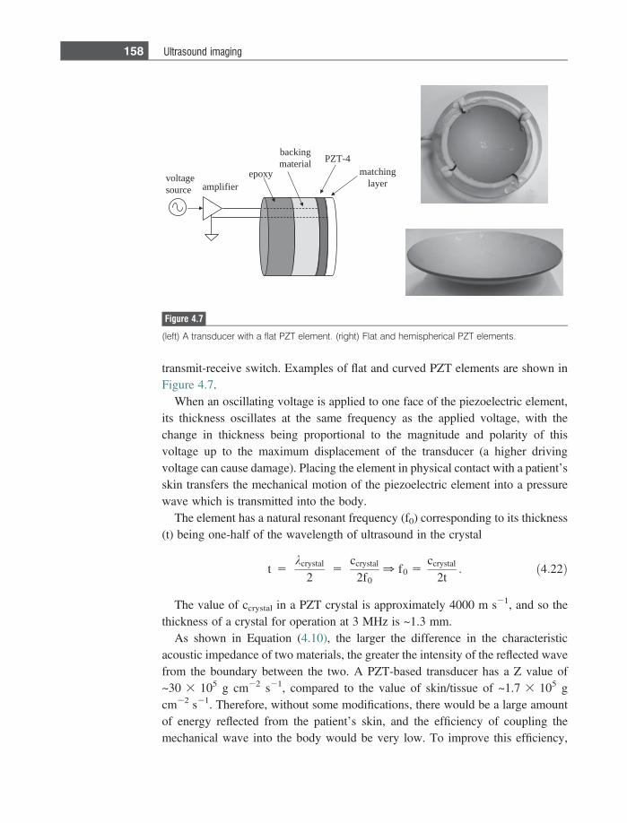
transmit-receive switch. Examples of flat and curved PZT elements are shown inFigure 4.7.
When an oscillating voltage is applied to one face of the piezoelectric element,its thickness oscillates at the same frequency as the applied voltage, with thechange in thickness being proportional to the magnitude and polarity of thisvoltage up to the maximum displacement of the transducer (a higher drivingvoltage can cause damage). Placing the element in physical contact with a patient’sskin transfers the mechanical motion of the piezoelectric element into a pressurewave which is transmitted into the body.
The element has a natural resonant frequency (f0) corresponding to its thickness(t) being one-half of the wavelength of ultrasound in the crystal
t 5kcrystal
25
ccrystal
2f00 f0 5
ccrystal
2t: ð4:22Þ
The value of ccrystal in a PZT crystal is approximately 4000 m s21, and so thethickness of a crystal for operation at 3 MHz is ~1.3 mm.
As shown in Equation (4.10), the larger the difference in the characteristicacoustic impedance of two materials, the greater the intensity of the reflected wavefrom the boundary between the two. A PZT-based transducer has a Z value of~30 3 105 g cm22 s21, compared to the value of skin/tissue of ~1.7 3 105 gcm22 s21. Therefore, without some modifications, there would be a large amountof energy reflected from the patient’s skin, and the efficiency of coupling themechanical wave into the body would be very low. To improve this efficiency,
epoxy
backingmaterial
matchinglayer
PZT-4
voltagesource amplifier
Figure 4.7
(left) A transducer with a flat PZT element. (right) Flat and hemispherical PZT elements.
158 Ultrasound imaging
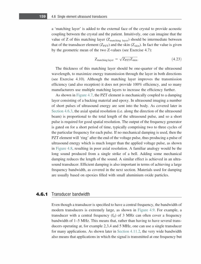
a ‘matching layer’ is added to the external face of the crystal to provide acousticcoupling between the crystal and the patient. Intuitively, one can imagine that thevalue of Z of this matching layer (Zmatching layer) should be intermediate betweenthat of the transducer element (ZPZT) and the skin (Zskin). In fact the value is givenby the geometric mean of the two Z-values (see Exercise 4.7):
Zmatching layer 5ffiffiffiffiffiffiffiffiffiffiffiffiffiffiffiffiffiffiZPZTZskinp
: ð4:23Þ
The thickness of this matching layer should be one-quarter of the ultrasoundwavelength, to maximize energy transmission through the layer in both directions(see Exercise 4.10). Although the matching layer improves the transmissionefficiency (and also reception) it does not provide 100% efficiency, and so manymanufacturers use multiple matching layers to increase the efficiency further.
As shown in Figure 4.7, the PZT element is mechanically coupled to a dampinglayer consisting of a backing material and epoxy. In ultrasound imaging a numberof short pulses of ultrasound energy are sent into the body. As covered later inSection 4.6.3, the axial spatial resolution (i.e. along the direction of the ultrasoundbeam) is proportional to the total length of the ultrasound pulse, and so a shortpulse is required for good spatial resolution. The output of the frequency generatoris gated on for a short period of time, typically comprising two to three cycles ofthe particular frequency for each pulse. If no mechanical damping is used, then thePZT element will ‘ring’ after the end of the voltage pulse, thus producing a pulse ofultrasound energy which is much longer than the applied voltage pulse, as shownin Figure 4.8, resulting in poor axial resolution. A familiar analogy would be thelong sound produced from a single strike of a bell. Adding some mechanicaldamping reduces the length of the sound. A similar effect is achieved in an ultra-sound transducer. Efficient damping is also important in terms of achieving a largefrequency bandwidth, as covered in the next section. Materials used for dampingare usually based on epoxies filled with small aluminium oxide particles.
4.6.1 Transducer bandwidth
Even though a transducer is specified to have a central frequency, the bandwidth ofmodern transducers is extremely large, as shown in Figure 4.9. For example, atransducer with a central frequency (f0) of 3 MHz can often cover a frequencybandwidth of 1–5 MHz. This means that, rather than having to have several trans-ducers operating at, for example 2,3,4 and 5 MHz, one can use a single transducerfor many applications. As shown later in Section 4.11.2, the very wide bandwidthalso means that applications in which the signal is transmitted at one frequency but
159 4.6 Single element ultrasound transducers
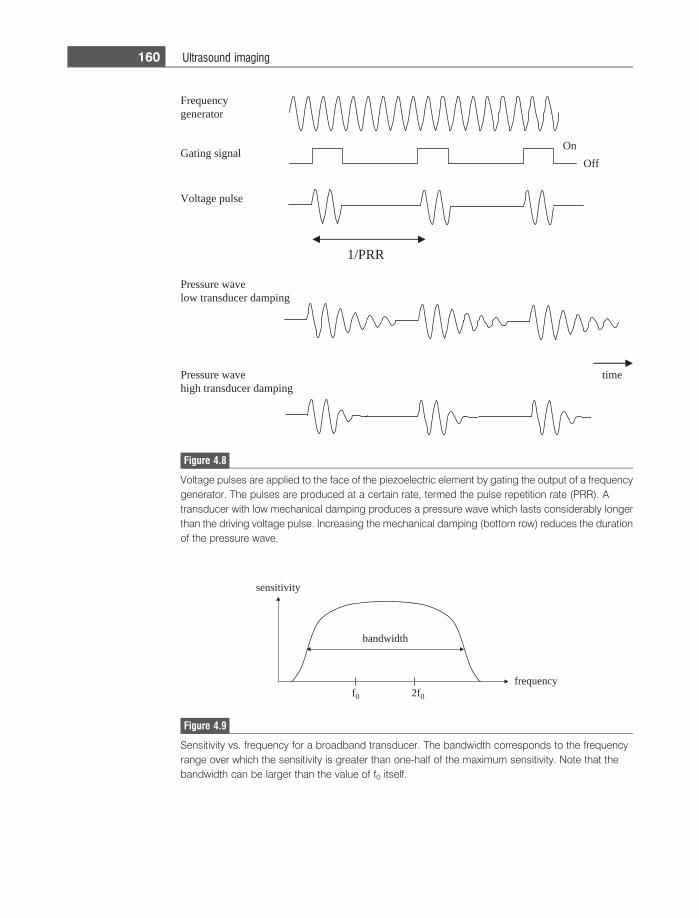
Pressure wave low transducer damping
On
timePressure wave high transducer damping
Frequency generator
Gating signal
1/PRR
Voltage pulse
Off
Figure 4.8
Voltage pulses are applied to the face of the piezoelectric element by gating the output of a frequencygenerator. The pulses are produced at a certain rate, termed the pulse repetition rate (PRR). Atransducer with low mechanical damping produces a pressure wave which lasts considerably longerthan the driving voltage pulse. Increasing the mechanical damping (bottom row) reduces the durationof the pressure wave.
f0 2f0
sensitivity
frequency
bandwidth
Figure 4.9
Sensitivity vs. frequency for a broadband transducer. The bandwidth corresponds to the frequencyrange over which the sensitivity is greater than one-half of the maximum sensitivity. Note that thebandwidth can be larger than the value of f0 itself.
160 Ultrasound imaging
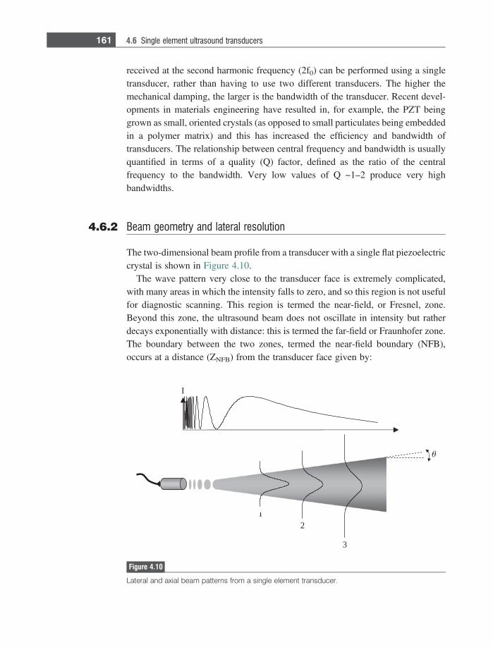
received at the second harmonic frequency (2f0) can be performed using a singletransducer, rather than having to use two different transducers. The higher themechanical damping, the larger is the bandwidth of the transducer. Recent devel-opments in materials engineering have resulted in, for example, the PZT beinggrown as small, oriented crystals (as opposed to small particulates being embeddedin a polymer matrix) and this has increased the efficiency and bandwidth oftransducers. The relationship between central frequency and bandwidth is usuallyquantified in terms of a quality (Q) factor, defined as the ratio of the centralfrequency to the bandwidth. Very low values of Q ~1–2 produce very highbandwidths.
4.6.2 Beam geometry and lateral resolution
The two-dimensional beam profile from a transducer with a single flat piezoelectriccrystal is shown in Figure 4.10.
The wave pattern very close to the transducer face is extremely complicated,with many areas in which the intensity falls to zero, and so this region is not usefulfor diagnostic scanning. This region is termed the near-field, or Fresnel, zone.Beyond this zone, the ultrasound beam does not oscillate in intensity but ratherdecays exponentially with distance: this is termed the far-field or Fraunhofer zone.The boundary between the two zones, termed the near-field boundary (NFB),occurs at a distance (ZNFB) from the transducer face given by:
12
3
I
Figure 4.10
Lateral and axial beam patterns from a single element transducer.
161 4.6 Single element ultrasound transducers

ZNFB �r2
k; ð4:24Þ
where r is the radius of the transducer, and k is the wavelength of the ultrasoundin tissue. At the NFB, the field has a lateral beamwidth which is approximatelyequal to the diameter of the transducer. Beyond the NFB, the beam diverges in thelateral direction, with the angle of deviation (h, shown in Figure 4.10) given by:
h 5 arcsin0:61k
r
� �: ð4:25Þ
Example 4.4 Calculate the position of the NFB for a transducer operating at 3 MHz, with acrystal diameter of 1 cm. What is the approximate beam width at a distance of 10cm from the transducer surface?
Solution Assuming that the speed of sound in tissue is 1540 m/s, the wavelength of a 3 MHzpulse of ultrasound is 1540/(33106) = 5.1331024 m ~0.05 cm. Therefore, theposition of the NFB is ~(0.25/0.05) ~5 cm from the tranducer surface.The divergent angle from Equation (4.25) is given by:
h ¼ arcsin0:61k
r
� �¼ arcsin
0:61crf
� �¼ arcsin
0:61 � 1540ms�1
0:005m � 3 3 106s�1
� �� 3:6�:
If one assumes that the beamwidth at the NFB is 1 cm, then the beamwidth at adistance of 10 cm (5 cm from the NFB) is given by:
1þ 5 tan 3:6oð Þ � 1:31 cm:
In the far-field, Figure 4.10 shows that the lateral beam shape is approximatelyGaussian. The lateral resolution is defined as the FWHM which is given by:
FWHM 5 2:36r; ð4:26Þ
where r is the standard deviation of the Gaussian function.It should also be noted that side-lobes are also produced by a single element
transducer, with the first zero of the side-lobe present at an angle u given by:
u ¼ arcsin0:61k
r
� �: ð4:27Þ
These side-lobes can introduce artifacts into an image if the lobes are back-scattered from tissue which is outside the region being studied.
162 Ultrasound imaging
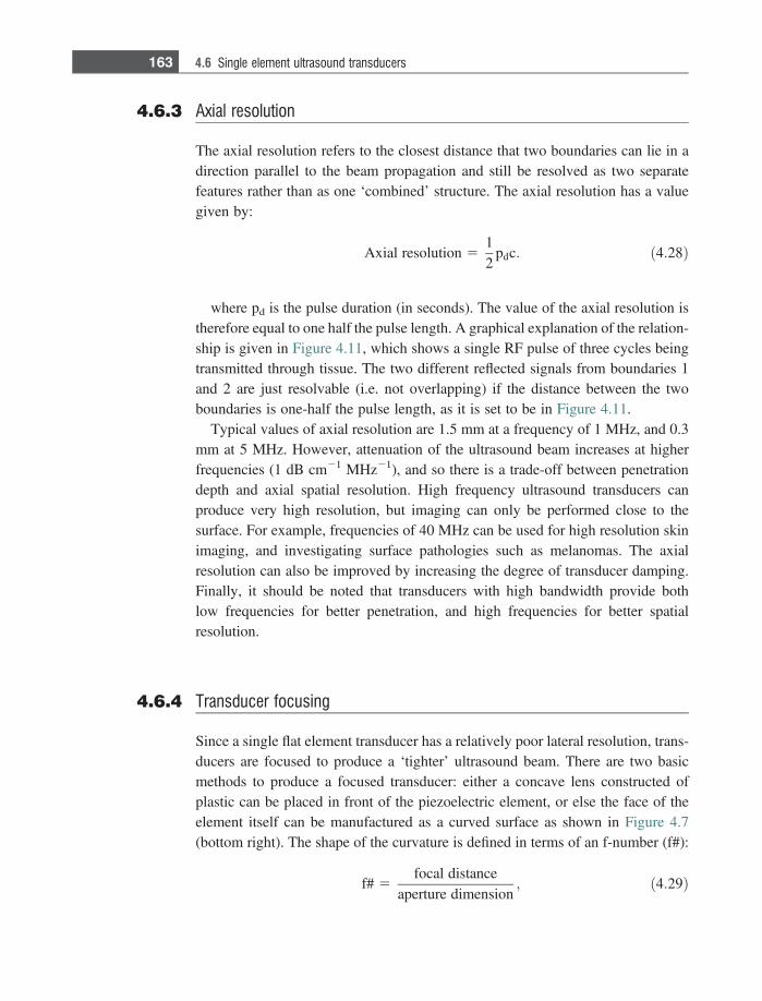
4.6.3 Axial resolution
The axial resolution refers to the closest distance that two boundaries can lie in adirection parallel to the beam propagation and still be resolved as two separatefeatures rather than as one ‘combined’ structure. The axial resolution has a valuegiven by:
Axial resolution 512
pdc: ð4:28Þ
where pd is the pulse duration (in seconds). The value of the axial resolution istherefore equal to one half the pulse length. A graphical explanation of the relation-ship is given in Figure 4.11, which shows a single RF pulse of three cycles beingtransmitted through tissue. The two different reflected signals from boundaries 1and 2 are just resolvable (i.e. not overlapping) if the distance between the twoboundaries is one-half the pulse length, as it is set to be in Figure 4.11.
Typical values of axial resolution are 1.5 mm at a frequency of 1 MHz, and 0.3mm at 5 MHz. However, attenuation of the ultrasound beam increases at higherfrequencies (1 dB cm21 MHz21), and so there is a trade-off between penetrationdepth and axial spatial resolution. High frequency ultrasound transducers canproduce very high resolution, but imaging can only be performed close to thesurface. For example, frequencies of 40 MHz can be used for high resolution skinimaging, and investigating surface pathologies such as melanomas. The axialresolution can also be improved by increasing the degree of transducer damping.Finally, it should be noted that transducers with high bandwidth provide bothlow frequencies for better penetration, and high frequencies for better spatialresolution.
4.6.4 Transducer focusing
Since a single flat element transducer has a relatively poor lateral resolution, trans-ducers are focused to produce a ‘tighter’ ultrasound beam. There are two basicmethods to produce a focused transducer: either a concave lens constructed ofplastic can be placed in front of the piezoelectric element, or else the face of theelement itself can be manufactured as a curved surface as shown in Figure 4.7(bottom right). The shape of the curvature is defined in terms of an f-number (f#):
f# 5focal distance
aperture dimension; ð4:29Þ
163 4.6 Single element ultrasound transducers
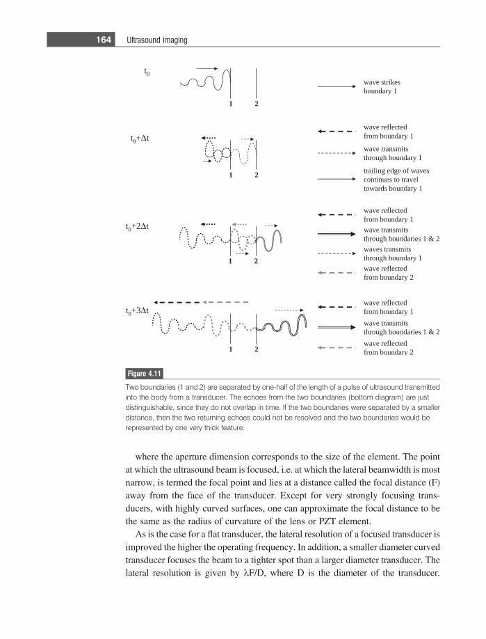
where the aperture dimension corresponds to the size of the element. The pointat which the ultrasound beam is focused, i.e. at which the lateral beamwidth is mostnarrow, is termed the focal point and lies at a distance called the focal distance (F)away from the face of the transducer. Except for very strongly focusing trans-ducers, with highly curved surfaces, one can approximate the focal distance to bethe same as the radius of curvature of the lens or PZT element.
As is the case for a flat transducer, the lateral resolution of a focused transducer isimproved the higher the operating frequency. In addition, a smaller diameter curvedtransducer focuses the beam to a tighter spot than a larger diameter transducer. Thelateral resolution is given by kF/D, where D is the diameter of the transducer.
wave strikesboundary 1
wave reflectedfrom boundary 1
wave transmitsthrough boundary 1
trailing edge of wavescontinues to traveltowards boundary 1
wave reflectedfrom boundary 1
wave transmitsthrough boundaries 1 & 2
waves transmitsthrough boundary 1
wave reflectedfrom boundary 2
wave reflectedfrom boundary 1
wave transmitsthrough boundaries 1 & 2
wave reflectedfrom boundary 2
t0
21
t0+ t
21
t0+2 t
21
t0+3 t
21
Figure 4.11
Two boundaries (1 and 2) are separated by one-half of the length of a pulse of ultrasound transmittedinto the body from a transducer. The echoes from the two boundaries (bottom diagram) are justdistinguishable, since they do not overlap in time. If the two boundaries were separated by a smallerdistance, then the two returning echoes could not be resolved and the two boundaries would berepresented by one very thick feature.
164 Ultrasound imaging
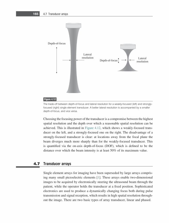
Choosing the focusing power of the transducer is a compromise between the highestspatial resolution and the depth over which a reasonable spatial resolution can beachieved. This is illustrated in Figure 4.12, which shows a weakly-focused trans-ducer on the left, and a strongly-focused one on the right. The disadvantage of astrongly-focused transducer is clear: at locations away from the focal plane thebeam diverges much more sharply than for the weakly-focused transducer. Thisis quantified via the on-axis depth-of-focus (DOF), which is defined to be thedistance over which the beam intensity is at least 50% of its maximum value.
4.7 Transducer arrays
Single element arrays for imaging have been superseded by large arrays compris-ing many small piezoelectric elements [1]. These arrays enable two-dimensionalimages to be acquired by electronically steering the ultrasound beam through thepatient, while the operator holds the transducer at a fixed position. Sophisticatedelectronics are used to produce a dynamically changing focus both during pulsetransmission and signal reception, which results in high spatial resolution through-out the image. There are two basic types of array transducer, linear and phased.
Depth-of-focus
Lateralresolution Lateral
resolutionDepth-of-focus
Figure 4.12
The trade-off between depth-of-focus and lateral resolution for a weakly-focused (left) and strongly-focused (right) single element transducer. A better lateral resolution is accompanied by a smallerdepth-of-focus, and vice versa.
165 4.7 Transducer arrays
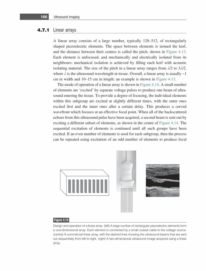
4.7.1 Linear arrays
A linear array consists of a large number, typically 128–512, of rectangularlyshaped piezoelectric elements. The space between elements is termed the kerf,and the distance between their centres is called the pitch, shown in Figure 4.13.Each element is unfocused, and mechanically and electrically isolated from itsneighbours: mechanical isolation is achieved by filling each kerf with acousticisolating material. The size of the pitch in a linear array ranges from k/2 to 3k/2,where k is the ultrasound wavelength in tissue. Overall, a linear array is usually ~1cm in width and 10–15 cm in length: an example is shown in Figure 4.13.
The mode of operation of a linear array is shown in Figure 4.14. A small numberof elements are ‘excited’ by separate voltage pulses to produce one beam of ultra-sound entering the tissue. To provide a degree of focusing, the individual elementswithin this subgroup are excited at slightly different times, with the outer onesexcited first and the inner ones after a certain delay. This produces a curvedwavefront which focuses at an effective focal point. When all of the backscatteredechoes from this ultrasound pulse have been acquired, a second beam is sent out byexciting a different subset of elements, as shown in the centre of Figure 4.14. Thesequential excitation of elements is continued until all such groups have beenexcited. If an even number of elements is used for each subgroup, then the processcan be repeated using excitation of an odd number of elements to produce focal
Figure 4.13
Design and operation of a linear array. (left) A large number of rectangular piezoelectric elements forma one-dimensional array. Each element is connected by a small coaxial cable to the voltage source.(centre) A commercial linear array, with the dashed lines showing the ultrasound beams that are sentout sequentially from left-to-right. (right) A two-dimensional ultrasound image acquired using a lineararray.
166 Ultrasound imaging
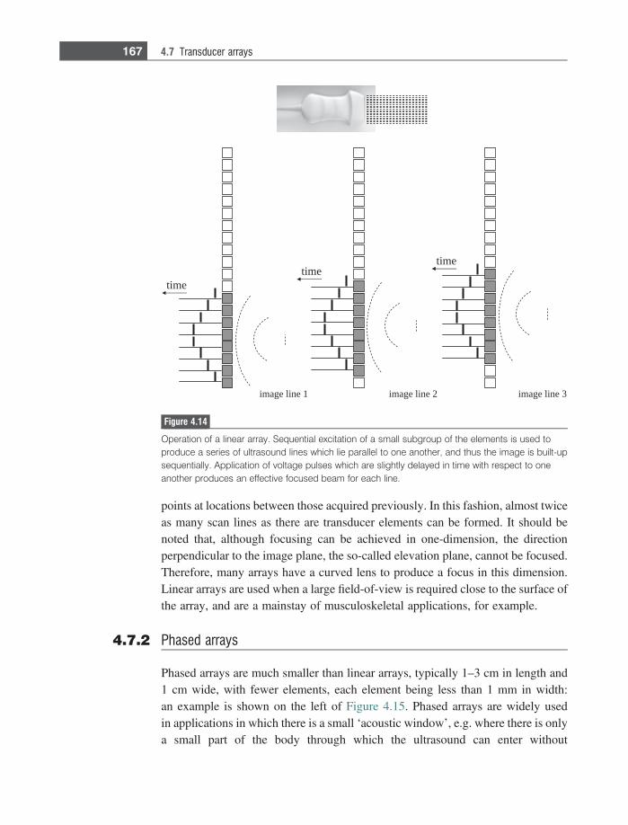
points at locations between those acquired previously. In this fashion, almost twiceas many scan lines as there are transducer elements can be formed. It should benoted that, although focusing can be achieved in one-dimension, the directionperpendicular to the image plane, the so-called elevation plane, cannot be focused.Therefore, many arrays have a curved lens to produce a focus in this dimension.Linear arrays are used when a large field-of-view is required close to the surface ofthe array, and are a mainstay of musculoskeletal applications, for example.
4.7.2 Phased arrays
Phased arrays are much smaller than linear arrays, typically 1–3 cm in length and1 cm wide, with fewer elements, each element being less than 1 mm in width:an example is shown on the left of Figure 4.15. Phased arrays are widely usedin applications in which there is a small ‘acoustic window’, e.g. where there is onlya small part of the body through which the ultrasound can enter without
timetime
time
3 enil egami2 enil egami1 enil egami
Figure 4.14
Operation of a linear array. Sequential excitation of a small subgroup of the elements is used toproduce a series of ultrasound lines which lie parallel to one another, and thus the image is built-upsequentially. Application of voltage pulses which are slightly delayed in time with respect to oneanother produces an effective focused beam for each line.
167 4.7 Transducer arrays
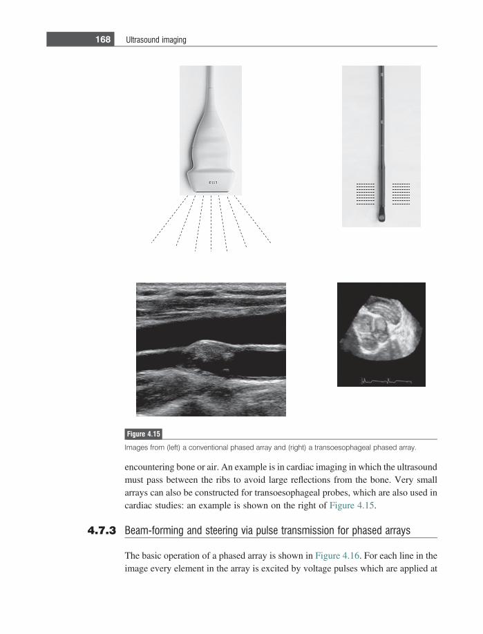
encountering bone or air. An example is in cardiac imaging in which the ultrasoundmust pass between the ribs to avoid large reflections from the bone. Very smallarrays can also be constructed for transoesophageal probes, which are also used incardiac studies: an example is shown on the right of Figure 4.15.
4.7.3 Beam-forming and steering via pulse transmission for phased arrays
The basic operation of a phased array is shown in Figure 4.16. For each line in theimage every element in the array is excited by voltage pulses which are applied at
Figure 4.15
Images from (left) a conventional phased array and (right) a transoesophageal phased array.
168 Ultrasound imaging
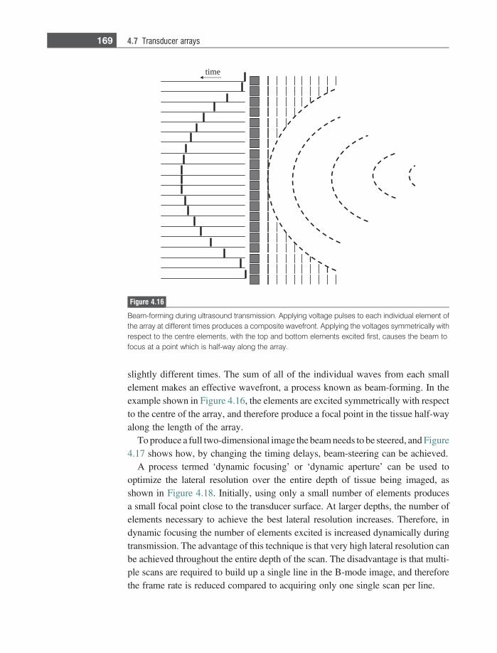
slightly different times. The sum of all of the individual waves from each smallelement makes an effective wavefront, a process known as beam-forming. In theexample shown in Figure 4.16, the elements are excited symmetrically with respectto the centre of the array, and therefore produce a focal point in the tissue half-wayalong the length of the array.
To produce a full two-dimensional image the beam needs to be steered, and Figure4.17 shows how, by changing the timing delays, beam-steering can be achieved.
A process termed ‘dynamic focusing’ or ‘dynamic aperture’ can be used tooptimize the lateral resolution over the entire depth of tissue being imaged, asshown in Figure 4.18. Initially, using only a small number of elements producesa small focal point close to the transducer surface. At larger depths, the number ofelements necessary to achieve the best lateral resolution increases. Therefore, indynamic focusing the number of elements excited is increased dynamically duringtransmission. The advantage of this technique is that very high lateral resolution canbe achieved throughout the entire depth of the scan. The disadvantage is that multi-ple scans are required to build up a single line in the B-mode image, and thereforethe frame rate is reduced compared to acquiring only one single scan per line.
time
Figure 4.16
Beam-forming during ultrasound transmission. Applying voltage pulses to each individual element ofthe array at different times produces a composite wavefront. Applying the voltages symmetrically withrespect to the centre elements, with the top and bottom elements excited first, causes the beam tofocus at a point which is half-way along the array.
169 4.7 Transducer arrays
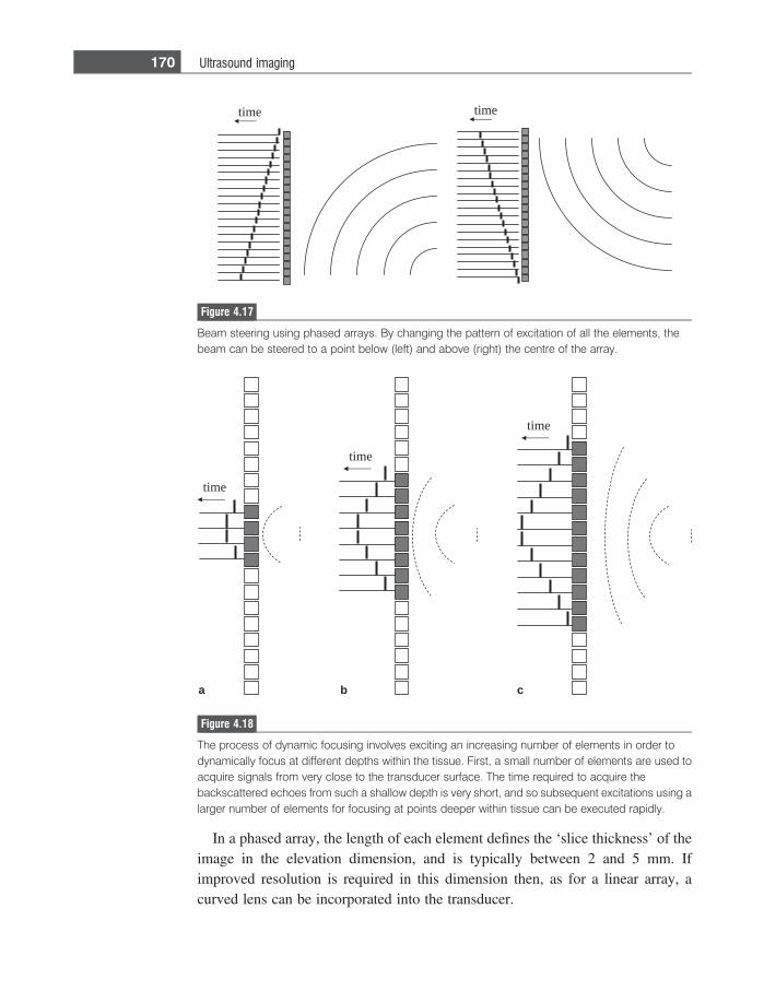
In a phased array, the length of each element defines the ‘slice thickness’ of theimage in the elevation dimension, and is typically between 2 and 5 mm. Ifimproved resolution is required in this dimension then, as for a linear array, acurved lens can be incorporated into the transducer.
time time
Figure 4.17
Beam steering using phased arrays. By changing the pattern of excitation of all the elements, thebeam can be steered to a point below (left) and above (right) the centre of the array.
time
time
time
a b c
Figure 4.18
The process of dynamic focusing involves exciting an increasing number of elements in order todynamically focus at different depths within the tissue. First, a small number of elements are used toacquire signals from very close to the transducer surface. The time required to acquire thebackscattered echoes from such a shallow depth is very short, and so subsequent excitations using alarger number of elements for focusing at points deeper within tissue can be executed rapidly.
170 Ultrasound imaging
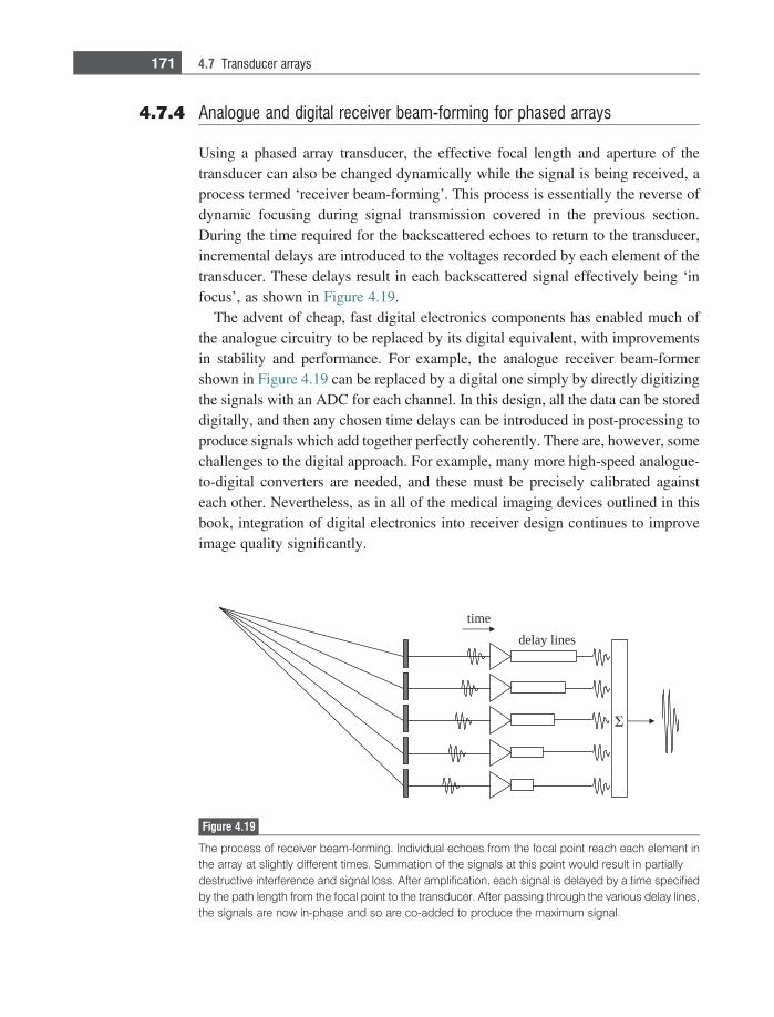
4.7.4 Analogue and digital receiver beam-forming for phased arrays
Using a phased array transducer, the effective focal length and aperture of thetransducer can also be changed dynamically while the signal is being received, aprocess termed ‘receiver beam-forming’. This process is essentially the reverse ofdynamic focusing during signal transmission covered in the previous section.During the time required for the backscattered echoes to return to the transducer,incremental delays are introduced to the voltages recorded by each element of thetransducer. These delays result in each backscattered signal effectively being ‘infocus’, as shown in Figure 4.19.
The advent of cheap, fast digital electronics components has enabled much ofthe analogue circuitry to be replaced by its digital equivalent, with improvementsin stability and performance. For example, the analogue receiver beam-formershown in Figure 4.19 can be replaced by a digital one simply by directly digitizingthe signals with an ADC for each channel. In this design, all the data can be storeddigitally, and then any chosen time delays can be introduced in post-processing toproduce signals which add together perfectly coherently. There are, however, somechallenges to the digital approach. For example, many more high-speed analogue-to-digital converters are needed, and these must be precisely calibrated againsteach other. Nevertheless, as in all of the medical imaging devices outlined in thisbook, integration of digital electronics into receiver design continues to improveimage quality significantly.
time
delay lines
Figure 4.19
The process of receiver beam-forming. Individual echoes from the focal point reach each element inthe array at slightly different times. Summation of the signals at this point would result in partiallydestructive interference and signal loss. After amplification, each signal is delayed by a time specifiedby the path length from the focal point to the transducer. After passing through the various delay lines,the signals are now in-phase and so are co-added to produce the maximum signal.
171 4.7 Transducer arrays
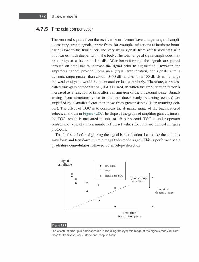
4.7.5 Time gain compensation
The summed signals from the receiver beam-former have a large range of ampli-tudes: very strong signals appear from, for example, reflections at fat/tissue boun-daries close to the transducer, and very weak signals from soft tissue/soft tissueboundaries much deeper within the body. The total range of signal amplitudes maybe as high as a factor of 100 dB. After beam-forming, the signals are passedthrough an amplifier to increase the signal prior to digitization. However, theamplifiers cannot provide linear gain (equal amplification) for signals with adynamic range greater than about 40–50 dB, and so for a 100 dB dynamic rangethe weaker signals would be attenuated or lost completely. Therefore, a processcalled time-gain compensation (TGC) is used, in which the amplification factor isincreased as a function of time after transmission of the ultrasound pulse. Signalsarising from structures close to the transducer (early returning echoes) areamplified by a smaller factor than those from greater depths (later returning ech-oes). The effect of TGC is to compress the dynamic range of the backscatteredechoes, as shown in Figure 4.20. The slope of the graph of amplifier gain vs. time isthe TGC, which is measured in units of dB per second. TGC is under operatorcontrol and typically has a number of preset values for standard clinical imagingprotocols.
The final step before digitizing the signal is rectification, i.e. to take the complexwaveform and transform it into a magnitude-mode signal. This is performed via aquadrature demodulator followed by envelope detection.
raw signal
signal after TGC
TGC
originaldynamic range
dynamic rangeafter TGC
signalamplitude
time aftertransmitted pulse
Figure 4.20
The effects of time-gain compensation in reducing the dynamic range of the signals received fromclose to the transducer surface and deep in tissue.
172 Ultrasound imaging
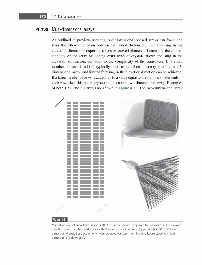
4.7.6 Multi-dimensional arrays
As outlined in previous sections, one-dimensional phased arrays can focus andsteer the ultrasound beam only in the lateral dimension, with focusing in theelevation dimension requiring a lens or curved elements. Increasing the dimen-sionality of the array by adding extra rows of crystals allows focusing in theelevation dimension, but adds to the complexity of the transducer. If a smallnumber of rows is added, typically three to ten, then the array is called a 1.5-dimensional array, and limited focusing in the elevation direction can be achieved.If a large number of rows is added, up to a value equal to the number of elements ineach row, then this geometry constitutes a true two-dimensional array. Examplesof both 1.5D and 2D arrays are shown in Figure 4.21. The two-dimensional array
Figure 4.21
Multi-dimensional array transducers. (left) A 1.5-dimensional array, with five elements in the elevationdirection which can be used to focus the beam in this dimension. (upper right) A 50 3 50 two-dimensional array transducer, which can be used for beam-forming and beam steering in twodimensions (below right).
173 4.7 Transducer arrays
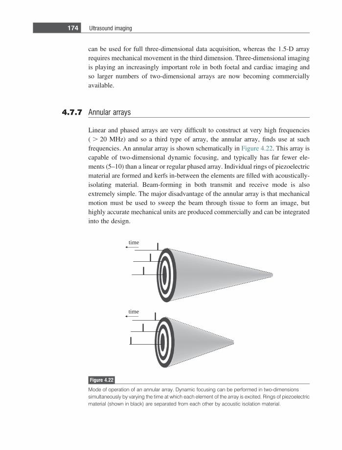
can be used for full three-dimensional data acquisition, whereas the 1.5-D arrayrequires mechanical movement in the third dimension. Three-dimensional imagingis playing an increasingly important role in both foetal and cardiac imaging andso larger numbers of two-dimensional arrays are now becoming commerciallyavailable.
4.7.7 Annular arrays
Linear and phased arrays are very difficult to construct at very high frequencies( . 20 MHz) and so a third type of array, the annular array, finds use at suchfrequencies. An annular array is shown schematically in Figure 4.22. This array iscapable of two-dimensional dynamic focusing, and typically has far fewer ele-ments (5–10) than a linear or regular phased array. Individual rings of piezoelectricmaterial are formed and kerfs in-between the elements are filled with acoustically-isolating material. Beam-forming in both transmit and receive mode is alsoextremely simple. The major disadvantage of the annular array is that mechanicalmotion must be used to sweep the beam through tissue to form an image, buthighly accurate mechanical units are produced commercially and can be integratedinto the design.
time
time
Figure 4.22
Mode of operation of an annular array. Dynamic focusing can be performed in two-dimensionssimultaneously by varying the time at which each element of the array is excited. Rings of piezoelectricmaterial (shown in black) are separated from each other by acoustic isolation material.
174 Ultrasound imaging
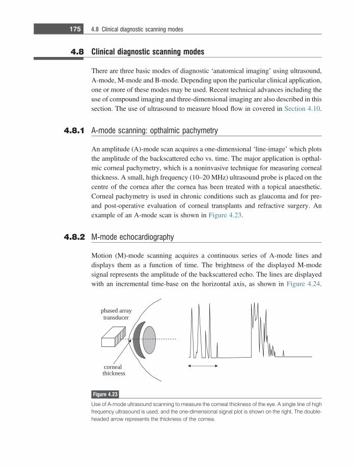
4.8 Clinical diagnostic scanning modes
There are three basic modes of diagnostic ‘anatomical imaging’ using ultrasound,A-mode, M-mode and B-mode. Depending upon the particular clinical application,one or more of these modes may be used. Recent technical advances including theuse of compound imaging and three-dimensional imaging are also described in thissection. The use of ultrasound to measure blood flow in covered in Section 4.10.
4.8.1 A-mode scanning: opthalmic pachymetry
An amplitude (A)-mode scan acquires a one-dimensional ‘line-image’ which plotsthe amplitude of the backscattered echo vs. time. The major application is opthal-mic corneal pachymetry, which is a noninvasive technique for measuring cornealthickness. A small, high frequency (10–20 MHz) ultrasound probe is placed on thecentre of the cornea after the cornea has been treated with a topical anaesthetic.Corneal pachymetry is used in chronic conditions such as glaucoma and for pre-and post-operative evaluation of corneal transplants and refractive surgery. Anexample of an A-mode scan is shown in Figure 4.23.
4.8.2 M-mode echocardiography
Motion (M)-mode scanning acquires a continuous series of A-mode lines anddisplays them as a function of time. The brightness of the displayed M-modesignal represents the amplitude of the backscattered echo. The lines are displayedwith an incremental time-base on the horizontal axis, as shown in Figure 4.24.
cornealthickness
phased arraytransducer
Figure 4.23
Use of A-mode ultrasound scanning to measure the corneal thickness of the eye. A single line of highfrequency ultrasound is used, and the one-dimensional signal plot is shown on the right. The double-headed arrow represents the thickness of the cornea.
175 4.8 Clinical diagnostic scanning modes
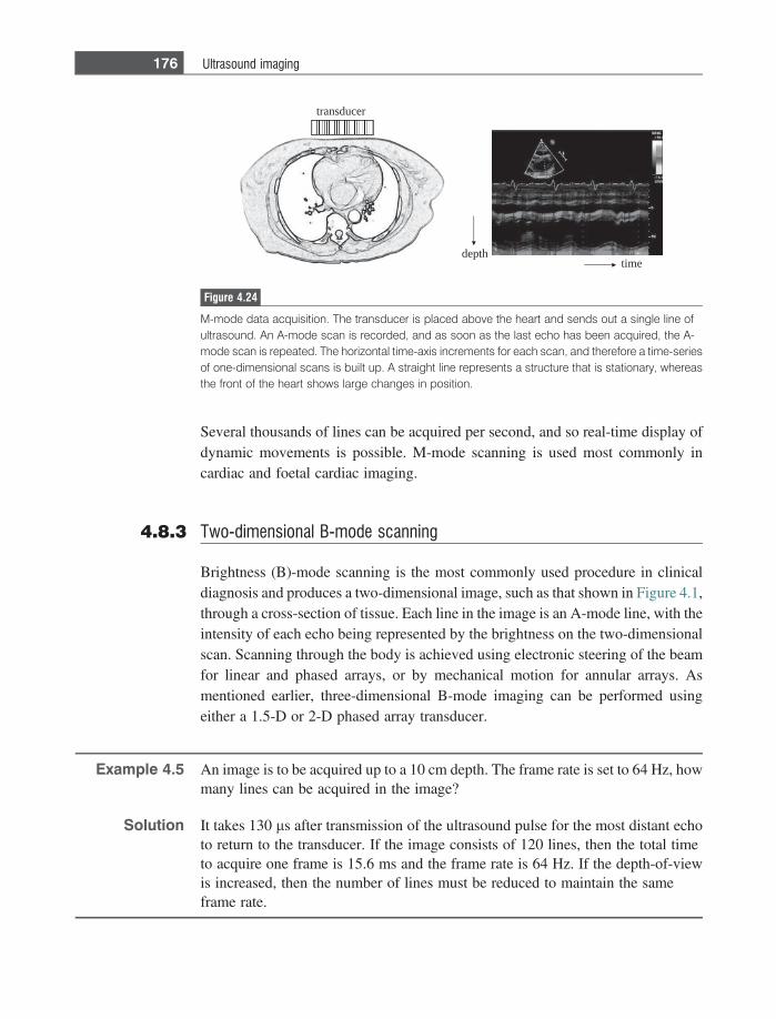
Several thousands of lines can be acquired per second, and so real-time display ofdynamic movements is possible. M-mode scanning is used most commonly incardiac and foetal cardiac imaging.
4.8.3 Two-dimensional B-mode scanning
Brightness (B)-mode scanning is the most commonly used procedure in clinicaldiagnosis and produces a two-dimensional image, such as that shown in Figure 4.1,through a cross-section of tissue. Each line in the image is an A-mode line, with theintensity of each echo being represented by the brightness on the two-dimensionalscan. Scanning through the body is achieved using electronic steering of the beamfor linear and phased arrays, or by mechanical motion for annular arrays. Asmentioned earlier, three-dimensional B-mode imaging can be performed usingeither a 1.5-D or 2-D phased array transducer.
Example 4.5 An image is to be acquired up to a 10 cm depth. The frame rate is set to 64 Hz, howmany lines can be acquired in the image?
Solution It takes 130 ls after transmission of the ultrasound pulse for the most distant echoto return to the transducer. If the image consists of 120 lines, then the total timeto acquire one frame is 15.6 ms and the frame rate is 64 Hz. If the depth-of-viewis increased, then the number of lines must be reduced to maintain the sameframe rate.
transducer
depthtime
Figure 4.24
M-mode data acquisition. The transducer is placed above the heart and sends out a single line ofultrasound. An A-mode scan is recorded, and as soon as the last echo has been acquired, the A-mode scan is repeated. The horizontal time-axis increments for each scan, and therefore a time-seriesof one-dimensional scans is built up. A straight line represents a structure that is stationary, whereasthe front of the heart shows large changes in position.
176 Ultrasound imaging
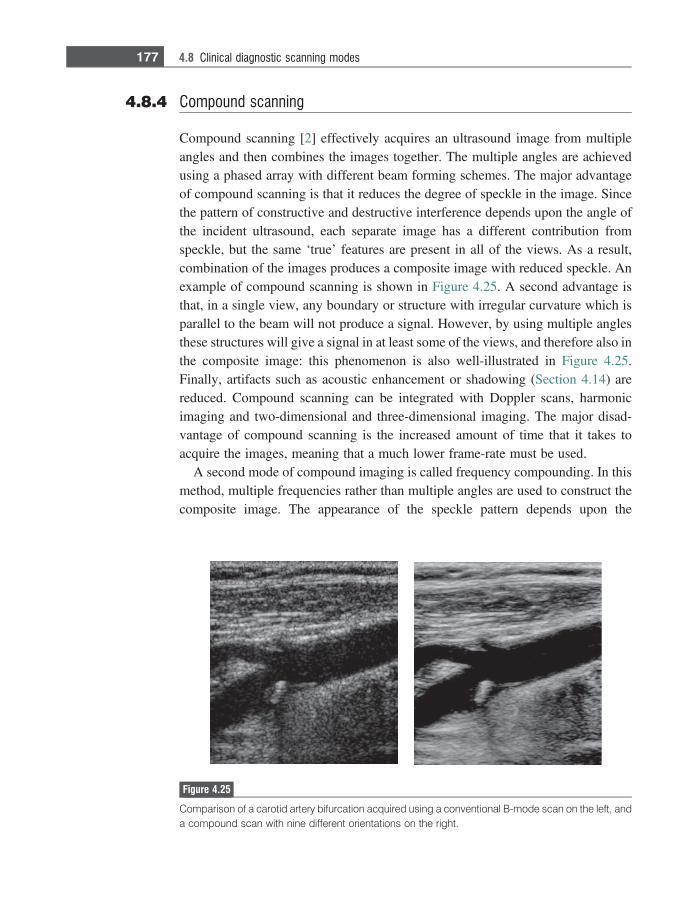
4.8.4 Compound scanning
Compound scanning [2] effectively acquires an ultrasound image from multipleangles and then combines the images together. The multiple angles are achievedusing a phased array with different beam forming schemes. The major advantageof compound scanning is that it reduces the degree of speckle in the image. Sincethe pattern of constructive and destructive interference depends upon the angle ofthe incident ultrasound, each separate image has a different contribution fromspeckle, but the same ‘true’ features are present in all of the views. As a result,combination of the images produces a composite image with reduced speckle. Anexample of compound scanning is shown in Figure 4.25. A second advantage isthat, in a single view, any boundary or structure with irregular curvature which isparallel to the beam will not produce a signal. However, by using multiple anglesthese structures will give a signal in at least some of the views, and therefore also inthe composite image: this phenomenon is also well-illustrated in Figure 4.25.Finally, artifacts such as acoustic enhancement or shadowing (Section 4.14) arereduced. Compound scanning can be integrated with Doppler scans, harmonicimaging and two-dimensional and three-dimensional imaging. The major disad-vantage of compound scanning is the increased amount of time that it takes toacquire the images, meaning that a much lower frame-rate must be used.
A second mode of compound imaging is called frequency compounding. In thismethod, multiple frequencies rather than multiple angles are used to construct thecomposite image. The appearance of the speckle pattern depends upon the
Figure 4.25
Comparison of a carotid artery bifurcation acquired using a conventional B-mode scan on the left, anda compound scan with nine different orientations on the right.
177 4.8 Clinical diagnostic scanning modes

frequency, and so does not add constructively between views. The transducermust, of course, have a large enough bandwidth to cover the frequency range.
4.9 Image characteristics
The major contributing factors to signal-to-noise, spatial resolution and contrast-to-noise have already been covered, and are summarized briefly here.
4.9.1 Signal-to-noise
The signal intensity of backscattered ultrasound signals is affected by:
(i) The intensity of the ultrasound pulse transmitted by the transducer – thehigher the intensity, the higher the amplitude of the detected signals. Thelonger the pulse, also the higher is the signal intensity. The intensity of theultrasound pulse is limited by FDA guidelines on the amount of energy that issafe to use during a scan. This topic is further discussed in Section 4.12.
(ii) The operating frequency of the transducer – the higher the frequency, thegreater the tissue attenuation, and therefore the lower the signal at large depthswithin the body.
(iii) The type of focusing used – the stronger the focusing at a particular point, thehigher the energy per unit area of the ultrasound wave, and the higher thesignal at that point. However, outside the depth-of-focus, the energy per unitarea is very low, as is the image SNR.
There are two major sources of noise in ultrasound images. The first, speckle,gives a granular appearance to what should appear as a homogeneous tissue. Thesecond contribution, termed ‘clutter’, corresponds to signals arising from side-lobes, grating lobes, multi-path reverberation, and tissue motion. Compound imag-ing can be used to reduce speckle, and harmonic imaging (covered later in Section4.11.2) can reduce clutter.
4.9.2 Spatial resolution
(i) Lateral resolution. For a single element transducer, the higher the degree offocusing the better is the spatial resolution at the focal spot, at the cost of areduced depth-of-focus. The higher the frequency, the better is the lateralresolution for both single element and phased array transducers.
178 Ultrasound imaging
(ii) Axial resolution. The axial resolution is given by one-half the length of theultrasound pulse. The higher the degree of damping, or the higher the oper-ating frequency, the shorter is the pulse and the better the axial resolution.
4.9.3 Contrast-to-noise
Factors which affect the SNR also contribute to the image CNR. Noise sourcessuch as clutter and speckle reduce the image CNR, especially for small pathologieswithin tissue.
4.10 Doppler ultrasound for blood flow measurements
Non-invasive measurements of blood flow are a critical component of diagnosis ina number of pathological conditions. Ultrasound can measure blood velocity bytaking advantage of the Doppler effect. This effect is familiar in everyday life as,for example, the higher frequency of an ambulance siren as it approaches thanwhen it is driving away. The ultrasound signal from blood has its origin in signalscatter from red blood cells (RBCs), which have a diameter of ~7–10 lm. Bloodflow, either towards or away from the transducer, alters the frequency of thebackscattered echoes compared to the transmitted ultrasound frequency from thetransducer. If blood is flowing towards the transducer the detected frequency ishigher than the transmitted frequency, and vice versa. Phased array transducers canbe used to localize blood flow measurements to a specified vessel, or region of avessel, by acquiring B-mode images. From these B-mode images the vessel sizecan be estimated, and measured blood velocities converted into blood flow values.Blood flow measurements can be very useful in detecting vessel stenoses, andunusual blood flow patterns.
In the example shown in Figure 4.26, the direction of blood flow is towards thetransducer, and therefore the effective frequency (fi
eff) of the incident ultrasoundbeam for the moving RBCs is higher than the actual frequency transmitted (fi):
feffi 5
c 1 v coshk
5fi c 1 v coshð Þ
c: ð4:30Þ
The same process occurs during signal reception, and so the frequency of theultrasound received by the transducer (frec) is given by:
frec 5feff
i c 1 v coshð Þc
5fi c 1 v coshð Þ2
c25 fi 1
2fiv coshc
1fiv2 cos2h
c2:
ð4:31Þ
179 4.10 Doppler ultrasound for blood flow measurements
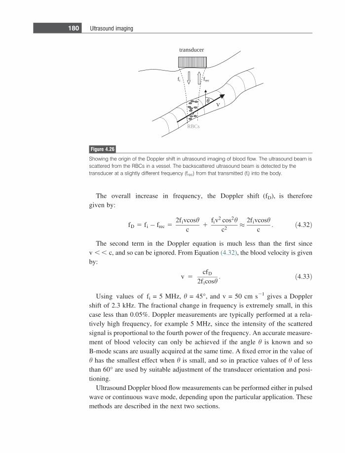
The overall increase in frequency, the Doppler shift (fD), is thereforegiven by:
fD 5 fi � frec 52fivcosh
c1
fiv2 cos2hc2
� 2fivcoshc
: ð4:32Þ
The second term in the Doppler equation is much less than the first sincev , , c, and so can be ignored. From Equation (4.32), the blood velocity is givenby:
v 5cfD
2ficosh: ð4:33Þ
Using values of fi = 5 MHz, h = 45�, and v = 50 cm s21 gives a Dopplershift of 2.3 kHz. The fractional change in frequency is extremely small, in thiscase less than 0.05%. Doppler measurements are typically performed at a rela-tively high frequency, for example 5 MHz, since the intensity of the scatteredsignal is proportional to the fourth power of the frequency. An accurate measure-ment of blood velocity can only be achieved if the angle h is known and soB-mode scans are usually acquired at the same time. A fixed error in the value ofh has the smallest effect when h is small, and so in practice values of h of lessthan 60� are used by suitable adjustment of the transducer orientation and posi-tioning.
Ultrasound Doppler blood flow measurements can be performed either in pulsedwave or continuous wave mode, depending upon the particular application. Thesemethods are described in the next two sections.
RBCs
V
fi frec
θ
transducer
Figure 4.26
Showing the origin of the Doppler shift in ultrasound imaging of blood flow. The ultrasound beam isscattered from the RBCs in a vessel. The backscattered ultrasound beam is detected by thetransducer at a slightly different frequency (frec) from that transmitted (fi) into the body.
180 Ultrasound imaging
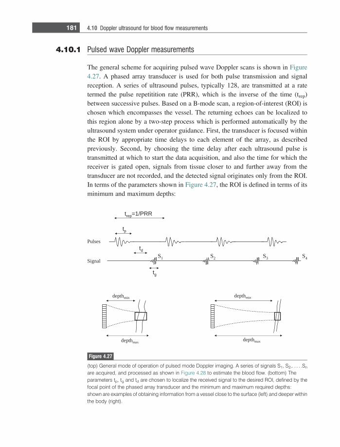
4.10.1 Pulsed wave Doppler measurements
The general scheme for acquiring pulsed wave Doppler scans is shown in Figure4.27. A phased array transducer is used for both pulse transmission and signalreception. A series of ultrasound pulses, typically 128, are transmitted at a ratetermed the pulse repetitition rate (PRR), which is the inverse of the time (trep)between successive pulses. Based on a B-mode scan, a region-of-interest (ROI) ischosen which encompasses the vessel. The returning echoes can be localized tothis region alone by a two-step process which is performed automatically by theultrasound system under operator guidance. First, the transducer is focused withinthe ROI by appropriate time delays to each element of the array, as describedpreviously. Second, by choosing the time delay after each ultrasound pulse istransmitted at which to start the data acquisition, and also the time for which thereceiver is gated open, signals from tissue closer to and further away from thetransducer are not recorded, and the detected signal originates only from the ROI.In terms of the parameters shown in Figure 4.27, the ROI is defined in terms of itsminimum and maximum depths:
Pulses
Signal
tp
td
tg
trep=1/PRR
depthmin
depthmax
depthmin
depthmax
S1 S2 S3 S4
Figure 4.27
(top) General mode of operation of pulsed mode Doppler imaging. A series of signals S1, S2,. . . . .Sn
are acquired, and processed as shown in Figure 4.28 to estimate the blood flow. (bottom) Theparameters tp, tg and td are chosen to localize the received signal to the desired ROI, defined by thefocal point of the phased array transducer and the minimum and maximum required depths:shown are examples of obtaining information from a vessel close to the surface (left) and deeper withinthe body (right).
181 4.10 Doppler ultrasound for blood flow measurements

depthmin 5c td � tp� �
2depthmax 5
c td þ tg� �
2: ð4:34Þ
Example 4.6 An ROI has been determined to be between 7 and 9 cm deep in the tissue. At whattime should the receiver be turned on after the end of pulse transmission, and forhow long should the receiver be gated on? The ultrasound pulse is 5 cycles at acentral frequency of 5 MHz.
Solution A train of ultrasound pulses is sent out, each pulse consisting of 5 cycles ofultrasound at a frequency of 5 MHz, resulting in a 1 ls long pulse. Assuming anultrasound velocity of 1540 m/s in tissue, the first part of Equation (4.34) gives:
0:07ðmÞ 51540ðms�1Þ � td � 1 3 10�6
� �ðsÞ
2;
from which td = 92 ls. Applying the second part of Equation (4.34):
0:09ðmÞ 51540ðms�1Þ � 92 3 10�6 þ tg
� �ðsÞ
2;
gives a gating-on time of ~25 ls.
Figure 4.28 shows the process of calculating the blood velocity within the ROIusing the pulsed Doppler technique. Signals S1, S2. . . . .Sn shown in Figure 4.27each have a different phase shift with respect to the first transmitted ultrasoundpulse. The amplitude of each time point within the signal is Fourier transformed togive a spectrum of the Doppler frequencies at each depth within the ROI. Thefrequency spectrum can then be converted into a velocity spectrum using Equation(4.32).
After the data have been processed, a ‘wall-filter’ is applied to the data toremove the very low frequency contributions from very slowly moving vesselsor tissue walls. The data are also passed through a quadrature detector so thatpositive and negative Doppler frequencies can be differentiated, thus enabling thedirection of flow to be determined unambiguously.
4.10.2 Duplex and triplex image acquisition
A typical Doppler image displays flow information combined with a B-mode scan.In a duplex scan the Doppler display is a colour-flow image, whereas in triplexscanning an additional Doppler spectral display is shown. A schematic Doppler
182 Ultrasound imaging
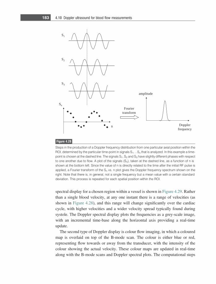
spectral display for a chosen region within a vessel is shown in Figure 4.29. Ratherthan a single blood velocity, at any one instant there is a range of velocities (asshown in Figure 4.28), and this range will change significantly over the cardiaccycle, with higher velocities and a wider velocity spread typically found duringsystole. The Doppler spectral display plots the frequencies as a grey-scale image,with an incremental time-base along the horizontal axis providing a real-timeupdate.
The second type of Doppler display is colour flow imaging, in which a colouredmap is overlaid on top of the B-mode scan. The colour is either blue or red,representing flow towards or away from the transducer, with the intensity of thecolour showing the actual velocity. These colour maps are updated in real-timealong with the B-mode scans and Doppler spectral plots. The computational steps
S1
S2
S3
Sn
n
Fouriertransform
Dopplerfrequency
amplitude
Figure 4.28
Steps in the production of a Doppler frequency distribution from one particular axial position within theROI, determined by the particular time-point in signals S1. . .Sn that is analyzed. In this example a time-point is chosen at the dashed line. The signals S1, S2 and S3 have slightly different phases with respectto one another due to flow. A plot of the signals (Sn), taken at the dashed line, as a function of n isshown at the bottom left. Since the value of n is directly related to the time after the initial RF pulse isapplied, a Fourier transform of the Sn vs. n plot gives the Doppler frequency spectrum shown on theright. Note that there is, in general, not a single frequency but a mean value with a certain standarddeviation. This process is repeated for each spatial position within the ROI.
183 4.10 Doppler ultrasound for blood flow measurements
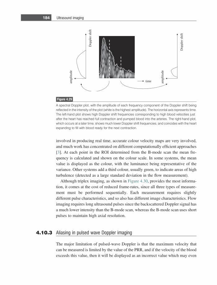
involved in producing real time, accurate colour velocity maps are very involved,and much work has concentrated on different computationally efficient approaches[3]. At each point in the ROI determined from the B-mode scan the mean fre-quency is calculated and shown on the colour scale. In some systems, the meanvalue is displayed as the colour, with the luminance being representative of thevariance. Other systems add a third colour, usually green, to indicate areas of highturbulence (detected as a large standard deviation in the flow measurement).
Although triplex imaging, as shown in Figure 4.30, provides the most informa-tion, it comes at the cost of reduced frame-rates, since all three types of measure-ment must be performed sequentially. Each measurement requires slightlydifferent pulse characteristics, and so also has different image characteristics. Flowimaging requires long ultrasound pulses since the backscattered Doppler signal hasa much lower intensity than the B-mode scan, whereas the B-mode scan uses shortpulses to maintain high axial resolution.
4.10.3 Aliasing in pulsed wave Doppler imaging
The major limitation of pulsed-wave Doppler is that the maximum velocity thatcan be measured is limited by the value of the PRR, and if the velocity of the bloodexceeds this value, then it will be displayed as an incorrect value which may even
ampl
itud
e
Dop
pler
shi
ft
Dop
pler
shi
ft
ampl
itud
e
time
Figure 4.29
A spectral Doppler plot, with the amplitude of each frequency component of the Doppler shift beingreflected in the intensity of the plot (white is the highest amplitude). The horizontal axis represents time.The left-hand plot shows high Doppler shift frequencies corresponding to high blood velocities justafter the heart has reached full contraction and pumped blood into the arteries. The right-hand plot,which occurs at a later time, shows much lower Doppler shift frequencies, and coincides with the heartexpanding to fill with blood ready for the next contraction.
184 Ultrasound imaging
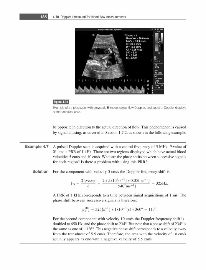
be opposite in direction to the actual direction of flow. This phenomenon is causedby signal aliasing, as covered in Section 1.7.2, as shown in the following example.
Example 4.7 A pulsed Doppler scan is acquired with a central frequency of 5 MHz, h value of0�, and a PRR of 1 kHz. There are two regions displayed which have actual bloodvelocities 5 cm/s and 10 cm/s. What are the phase shifts between successive signalsfor each region? Is there a problem with using this PRR?
Solution For the component with velocity 5 cm/s the Doppler frequency shift is:
fD 52fivcosh
c5
2 � 5x10⁶ðs�1Þ � 0:05ðms�1Þ1540 ms�1ð Þ 5 325Hz:
A PRR of 1 kHz corresponds to a time between signal acquisitions of 1 ms. Thephase shift between successive signals is therefore:
u 0� �
5 325 s�1� �
� 1x10�3 sð Þ � 360o 5 1170:
For the second component with velocity 10 cm/s the Doppler frequency shift isdoubled to 650 Hz, and the phase shift to 234�. But note that a phase shift of 234� isthe same as one of 2126�. This negative phase shift corresponds to a velocity awayfrom the transducer of 5.5 cm/s. Therefore, the area with the velocity of 10 cm/sactually appears as one with a negative velocity of 5.5 cm/s.
Figure 4.30
Example of a triplex scan, with greyscale B-mode, colour flow Doppler, and spectral Doppler displaysof the umbilical cord.
185 4.10 Doppler ultrasound for blood flow measurements
It is clear from the above example that signal aliasing occurs when the phase shiftduring each delay between successive pulses (1/PRR) is greater than 180�. Giventhis condition, the maximum Doppler frequency shift (fmax) that can be measured is:
fmax 51
2trep5
PRR2
: ð4:35Þ
The corresponding value of the maximum blood velocity, vmax, that can bemeasured without aliasing can be derived from Equation (4.32) setting cos h = 1:
vmax 5cfmax
2fi5
PRRð Þc4fi
: ð4:36Þ
The value of the PRR also determines the maximum depth, dmax, from whichflow can be measured, with a value of dmax given by:
dmax 5ctrep
25
c2PRR
5c2
8fivmax: ð4:37Þ
If aliasing is suspected in a pulsed-mode Doppler image, the system can be beturned either to power Doppler mode (described below) or to continuous-waveDoppler mode, described in Section 4.10.5, to confirm if this is in fact the case.
4.10.4 Power Doppler
Another potential limitation in measuring colour Doppler shifts occurs when asubstantial portion of a vessel lies parallel to the face of the phased array transducer.In this case, one section of the colour velocity image shows flow towards the trans-ducer, and the other shows flow away from the transducer. Directly below the trans-ducer there is an area of very low signal. This effect can be removed by using the‘power Doppler’ mode [4], in which the area under the magnitude of the Dopplersignal is integrated to give the ‘Doppler power’. In this process both positive andnegative Doppler frequencies give a positive integrated power, and therefore signalvoids are removed. Aliasing artifacts at high flow rates are also eliminated since theintegral of an aliased signal is the same as that of a non-aliased signal. The majordisadvantage with power Doppler is the loss of directional information.
4.10.5 Continuous wave Doppler measurements
CW Doppler measurements can be used when there is no need to localize exactlythe source of the Doppler shifts. Many modern ultrasound systems can acquire
186 Ultrasound imaging
both CW and PW Doppler data using the same phased array transducer. In CWmode the array is ‘split’ into two sections, one which transmits a continuous pulseof ultrasound, and the other which receives the backscattered signals. The area inwhich blood flow is detected is defined by the overlap of the areas defined by thetransmission and reception beam-forming settings. The measured blood velocityis the average value over the entire sensitive region. In order to determine thedirection of flow (towards or away from the transducer) a quadrature detectormust be used. The main advantages of CW Doppler over PW Doppler methodsis that the method is neither limited to a maximum depth, nor to a maximummeasurable velocity. As with PW Doppler, a triplex display showing a CWDoppler image, Doppler spectral plot and B-mode scan is commonly used indiagnostic scans.
4.11 Ultrasound contrast agents
Contrast agents for ultrasound imaging comprise different types and formulationsof microbubbles or microspheres [5], and are used primarily for echocardiographyand Doppler imaging. In cardiac imaging they can be used for ventricular opaci-fication, the assessment of left ventricular volume, systolic function, and delinea-tion of the endocardial structures. By enhancing the signal intensity of Dopplerultrasound, they also make possible measurements of blood perfusion in the heartand other organs such as the liver.
4.11.1 Microbubbles
Currently there are two ultrasound agents, SonoVue and Optison, approved forworldwide clinical use. SonoVue is a microbubble which is coated with phospho-lipid monolayers and contains sulphur hexafluoride gas. Optison consists of micro-bubbles which contain perfluoropropane gas within a cross-linked serum albumenmicrosphere. The shells of these microbubbles are a few tens of nanometres thick,the bubble diameter being between 2 and 10 lm, see Figure 4.31. These micro-spheres are packaged as freeze-dried powders which can be rehydrated in phys-iological saline solution just before they are to be injected into the patient’sbloodstream. There are many other types of microbubble in the late stages ofclinical testing, with the main differences being in the particular gaseous coreand exact make-up of the microbubble shell. The reason for needing an outer shell,rather than simply using a bubble of gas, is that there is a very high surface tensionat the boundary between the microbubble and surrounding liquid: without the
187 4.11 Ultrasound contrast agents
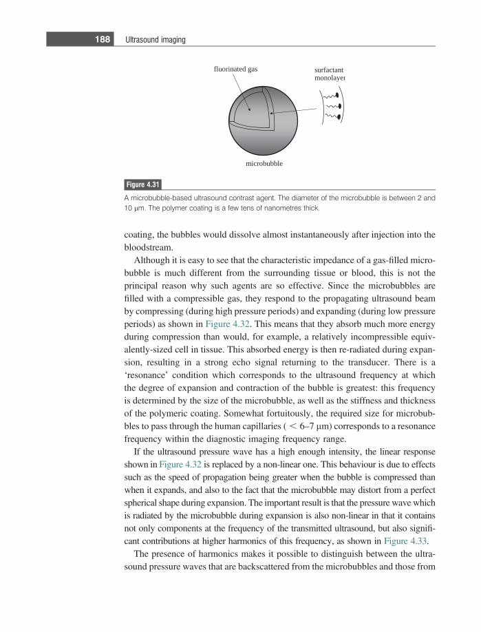
coating, the bubbles would dissolve almost instantaneously after injection into thebloodstream.
Although it is easy to see that the characteristic impedance of a gas-filled micro-bubble is much different from the surrounding tissue or blood, this is not theprincipal reason why such agents are so effective. Since the microbubbles arefilled with a compressible gas, they respond to the propagating ultrasound beamby compressing (during high pressure periods) and expanding (during low pressureperiods) as shown in Figure 4.32. This means that they absorb much more energyduring compression than would, for example, a relatively incompressible equiv-alently-sized cell in tissue. This absorbed energy is then re-radiated during expan-sion, resulting in a strong echo signal returning to the transducer. There is a‘resonance’ condition which corresponds to the ultrasound frequency at whichthe degree of expansion and contraction of the bubble is greatest: this frequencyis determined by the size of the microbubble, as well as the stiffness and thicknessof the polymeric coating. Somewhat fortuitously, the required size for microbub-bles to pass through the human capillaries ( , 6–7 lm) corresponds to a resonancefrequency within the diagnostic imaging frequency range.
If the ultrasound pressure wave has a high enough intensity, the linear responseshown in Figure 4.32 is replaced by a non-linear one. This behaviour is due to effectssuch as the speed of propagation being greater when the bubble is compressed thanwhen it expands, and also to the fact that the microbubble may distort from a perfectspherical shape during expansion. The important result is that the pressure wave whichis radiated by the microbubble during expansion is also non-linear in that it containsnot only components at the frequency of the transmitted ultrasound, but also signifi-cant contributions at higher harmonics of this frequency, as shown in Figure 4.33.
The presence of harmonics makes it possible to distinguish between the ultra-sound pressure waves that are backscattered from the microbubbles and those from
fluorinated gas surfactantmonolayer
microbubble
Figure 4.31
A microbubble-based ultrasound contrast agent. The diameter of the microbubble is between 2 and10 lm. The polymer coating is a few tens of nanometres thick.
188 Ultrasound imaging
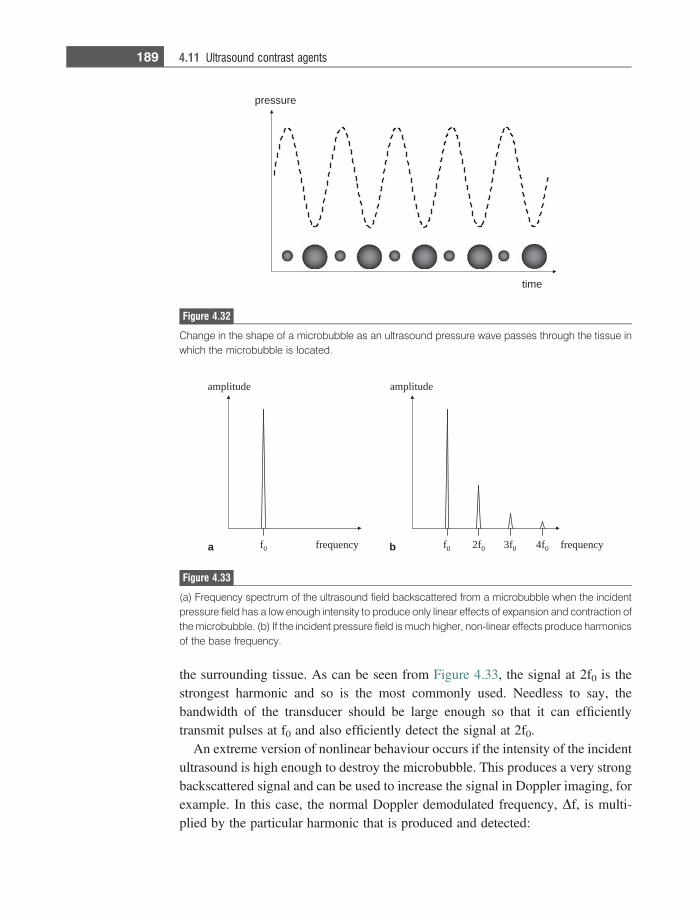
the surrounding tissue. As can be seen from Figure 4.33, the signal at 2f0 is thestrongest harmonic and so is the most commonly used. Needless to say, thebandwidth of the transducer should be large enough so that it can efficientlytransmit pulses at f0 and also efficiently detect the signal at 2f0.
An extreme version of nonlinear behaviour occurs if the intensity of the incidentultrasound is high enough to destroy the microbubble. This produces a very strongbackscattered signal and can be used to increase the signal in Doppler imaging, forexample. In this case, the normal Doppler demodulated frequency, Df, is multi-plied by the particular harmonic that is produced and detected:
f0 f0 2f0 3f0 4f0
edutilpmaedutilpma
frequencyfrequencya b
Figure 4.33
(a) Frequency spectrum of the ultrasound field backscattered from a microbubble when the incidentpressure field has a low enough intensity to produce only linear effects of expansion and contraction ofthe microbubble. (b) If the incident pressure field is much higher, non-linear effects produce harmonicsof the base frequency.
pressure
time
Figure 4.32
Change in the shape of a microbubble as an ultrasound pressure wave passes through the tissue inwhich the microbubble is located.
189 4.11 Ultrasound contrast agents
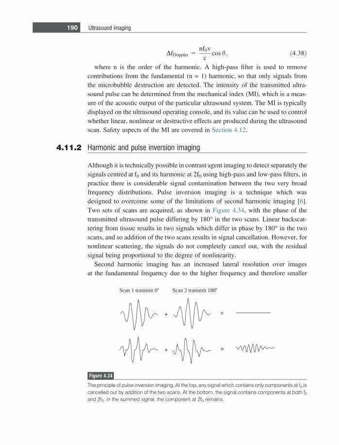
DfDoppler 5nf0v
ccos h; ð4:38Þ
where n is the order of the harmonic. A high-pass filter is used to removecontributions from the fundamental (n = 1) harmonic, so that only signals fromthe microbubble destruction are detected. The intensity of the transmitted ultra-sound pulse can be determined from the mechanical index (MI), which is a meas-ure of the acoustic output of the particular ultrasound system. The MI is typicallydisplayed on the ultrasound operating console, and its value can be used to controlwhether linear, nonlinear or destructive effects are produced during the ultrasoundscan. Safety aspects of the MI are covered in Section 4.12.
4.11.2 Harmonic and pulse inversion imaging
Although it is technically possible in contrast agent imaging to detect separately thesignals centred at f0 and its harmonic at 2f0 using high-pass and low-pass filters, inpractice there is considerable signal contamination between the two very broadfrequency distributions. Pulse inversion imaging is a technique which wasdesigned to overcome some of the limitations of second harmonic imaging [6].Two sets of scans are acquired, as shown in Figure 4.34, with the phase of thetransmitted ultrasound pulse differing by 180� in the two scans. Linear backscat-tering from tissue results in two signals which differ in phase by 180� in the twoscans, and so addition of the two scans results in signal cancellation. However, fornonlinear scattering, the signals do not completely cancel out, with the residualsignal being proportional to the degree of nonlinearity.
Second harmonic imaging has an increased lateral resolution over imagesat the fundamental frequency due to the higher frequency and therefore smaller
+ =
+ =
Scan 1 transmit 0o Scan 2 transmit 180o
Figure 4.34
The principle of pulse inversion imaging. At the top, any signal which contains only components at f0 iscancelled out by addition of the two scans. At the bottom, the signal contains components at both f0and 2f0: in the summed signal, the component at 2f0 remains.
190 Ultrasound imaging
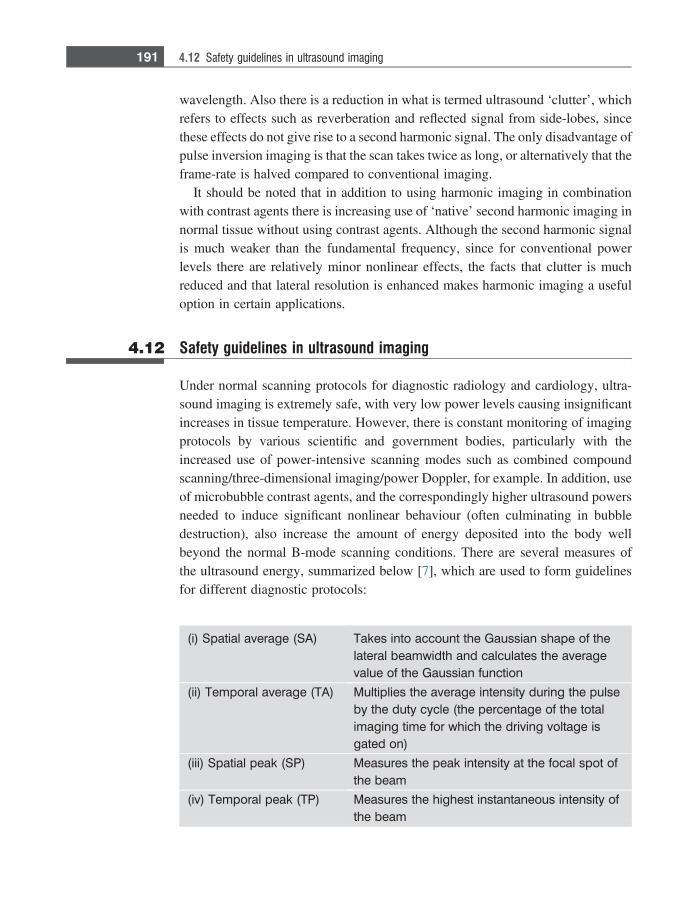
wavelength. Also there is a reduction in what is termed ultrasound ‘clutter’, whichrefers to effects such as reverberation and reflected signal from side-lobes, sincethese effects do not give rise to a second harmonic signal. The only disadvantage ofpulse inversion imaging is that the scan takes twice as long, or alternatively that theframe-rate is halved compared to conventional imaging.
It should be noted that in addition to using harmonic imaging in combinationwith contrast agents there is increasing use of ‘native’ second harmonic imaging innormal tissue without using contrast agents. Although the second harmonic signalis much weaker than the fundamental frequency, since for conventional powerlevels there are relatively minor nonlinear effects, the facts that clutter is muchreduced and that lateral resolution is enhanced makes harmonic imaging a usefuloption in certain applications.
4.12 Safety guidelines in ultrasound imaging
Under normal scanning protocols for diagnostic radiology and cardiology, ultra-sound imaging is extremely safe, with very low power levels causing insignificantincreases in tissue temperature. However, there is constant monitoring of imagingprotocols by various scientific and government bodies, particularly with theincreased use of power-intensive scanning modes such as combined compoundscanning/three-dimensional imaging/power Doppler, for example. In addition, useof microbubble contrast agents, and the correspondingly higher ultrasound powersneeded to induce significant nonlinear behaviour (often culminating in bubbledestruction), also increase the amount of energy deposited into the body wellbeyond the normal B-mode scanning conditions. There are several measures ofthe ultrasound energy, summarized below [7], which are used to form guidelinesfor different diagnostic protocols:
(i) Spatial average (SA) Takes into account the Gaussian shape of thelateral beamwidth and calculates the averagevalue of the Gaussian function
(ii) Temporal average (TA) Multiplies the average intensity during the pulseby the duty cycle (the percentage of the totalimaging time for which the driving voltage isgated on)
(iii) Spatial peak (SP) Measures the peak intensity at the focal spot ofthe beam
(iv) Temporal peak (TP) Measures the highest instantaneous intensity ofthe beam
191 4.12 Safety guidelines in ultrasound imaging
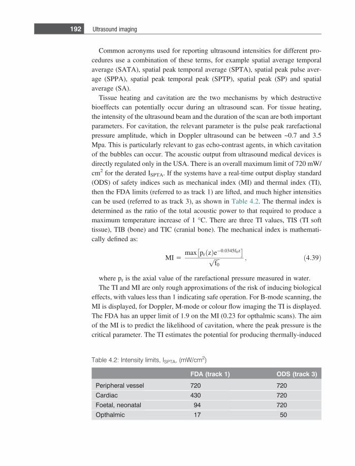
Common acronyms used for reporting ultrasound intensities for different pro-cedures use a combination of these terms, for example spatial average temporalaverage (SATA), spatial peak temporal average (SPTA), spatial peak pulse aver-age (SPPA), spatial peak temporal peak (SPTP), spatial peak (SP) and spatialaverage (SA).
Tissue heating and cavitation are the two mechanisms by which destructivebioeffects can potentially occur during an ultrasound scan. For tissue heating,the intensity of the ultrasound beam and the duration of the scan are both importantparameters. For cavitation, the relevant parameter is the pulse peak rarefactionalpressure amplitude, which in Doppler ultrasound can be between ~0.7 and 3.5Mpa. This is particularly relevant to gas echo-contrast agents, in which cavitationof the bubbles can occur. The acoustic output from ultrasound medical devices isdirectly regulated only in the USA. There is an overall maximum limit of 720 mW/cm2 for the derated ISPTA. If the systems have a real-time output display standard(ODS) of safety indices such as mechanical index (MI) and thermal index (TI),then the FDA limits (referred to as track 1) are lifted, and much higher intensitiescan be used (referred to as track 3), as shown in Table 4.2. The thermal index isdetermined as the ratio of the total acoustic power to that required to produce amaximum temperature increase of 1 �C. There are three TI values, TIS (TI softtissue), TIB (bone) and TIC (cranial bone). The mechanical index is mathemati-cally defined as:
MI 5max pr zð Þe�0:0345f0z
� �ffiffiffiffif0p ; ð4:39Þ
where pr is the axial value of the rarefactional pressure measured in water.The TI and MI are only rough approximations of the risk of inducing biological
effects, with values less than 1 indicating safe operation. For B-mode scanning, theMI is displayed, for Doppler, M-mode or colour flow imaging the TI is displayed.The FDA has an upper limit of 1.9 on the MI (0.23 for opthalmic scans). The aimof the MI is to predict the likelihood of cavitation, where the peak pressure is thecritical parameter. The TI estimates the potential for producing thermally-induced
Table 4.2: Intensity limits, ISPTA, (mW/cm2)
FDA (track 1) ODS (track 3)
Peripheral vessel 720 720
Cardiac 430 720
Foetal, neonatal 94 720
Opthalmic 17 50
192 Ultrasound imaging
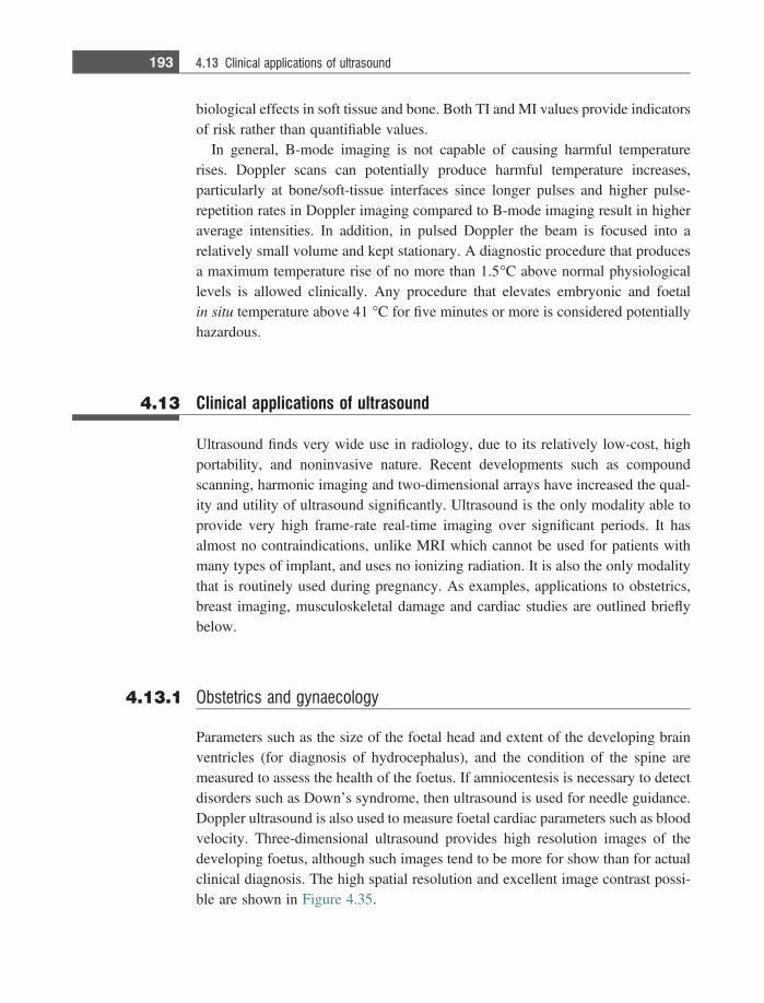
biological effects in soft tissue and bone. Both TI and MI values provide indicatorsof risk rather than quantifiable values.
In general, B-mode imaging is not capable of causing harmful temperaturerises. Doppler scans can potentially produce harmful temperature increases,particularly at bone/soft-tissue interfaces since longer pulses and higher pulse-repetition rates in Doppler imaging compared to B-mode imaging result in higheraverage intensities. In addition, in pulsed Doppler the beam is focused into arelatively small volume and kept stationary. A diagnostic procedure that producesa maximum temperature rise of no more than 1.5�C above normal physiologicallevels is allowed clinically. Any procedure that elevates embryonic and foetalin situ temperature above 41 �C for five minutes or more is considered potentiallyhazardous.
4.13 Clinical applications of ultrasound
Ultrasound finds very wide use in radiology, due to its relatively low-cost, highportability, and noninvasive nature. Recent developments such as compoundscanning, harmonic imaging and two-dimensional arrays have increased the qual-ity and utility of ultrasound significantly. Ultrasound is the only modality able toprovide very high frame-rate real-time imaging over significant periods. It hasalmost no contraindications, unlike MRI which cannot be used for patients withmany types of implant, and uses no ionizing radiation. It is also the only modalitythat is routinely used during pregnancy. As examples, applications to obstetrics,breast imaging, musculoskeletal damage and cardiac studies are outlined brieflybelow.
4.13.1 Obstetrics and gynaecology
Parameters such as the size of the foetal head and extent of the developing brainventricles (for diagnosis of hydrocephalus), and the condition of the spine aremeasured to assess the health of the foetus. If amniocentesis is necessary to detectdisorders such as Down’s syndrome, then ultrasound is used for needle guidance.Doppler ultrasound is also used to measure foetal cardiac parameters such as bloodvelocity. Three-dimensional ultrasound provides high resolution images of thedeveloping foetus, although such images tend to be more for show than for actualclinical diagnosis. The high spatial resolution and excellent image contrast possi-ble are shown in Figure 4.35.
193 4.13 Clinical applications of ultrasound
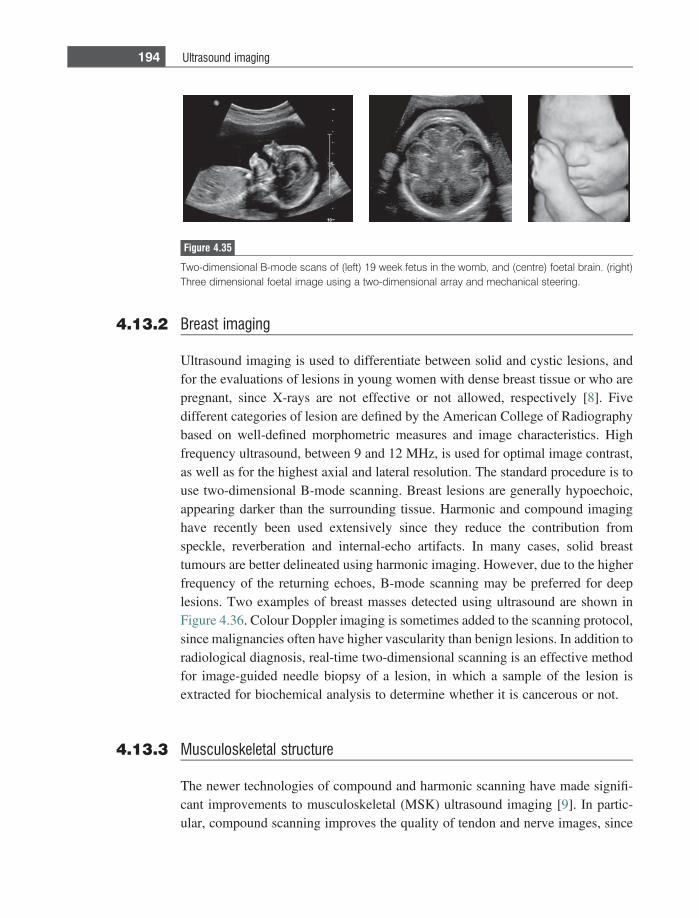
4.13.2 Breast imaging
Ultrasound imaging is used to differentiate between solid and cystic lesions, andfor the evaluations of lesions in young women with dense breast tissue or who arepregnant, since X-rays are not effective or not allowed, respectively [8]. Fivedifferent categories of lesion are defined by the American College of Radiographybased on well-defined morphometric measures and image characteristics. Highfrequency ultrasound, between 9 and 12 MHz, is used for optimal image contrast,as well as for the highest axial and lateral resolution. The standard procedure is touse two-dimensional B-mode scanning. Breast lesions are generally hypoechoic,appearing darker than the surrounding tissue. Harmonic and compound imaginghave recently been used extensively since they reduce the contribution fromspeckle, reverberation and internal-echo artifacts. In many cases, solid breasttumours are better delineated using harmonic imaging. However, due to the higherfrequency of the returning echoes, B-mode scanning may be preferred for deeplesions. Two examples of breast masses detected using ultrasound are shown inFigure 4.36. Colour Doppler imaging is sometimes added to the scanning protocol,since malignancies often have higher vascularity than benign lesions. In addition toradiological diagnosis, real-time two-dimensional scanning is an effective methodfor image-guided needle biopsy of a lesion, in which a sample of the lesion isextracted for biochemical analysis to determine whether it is cancerous or not.
4.13.3 Musculoskeletal structure
The newer technologies of compound and harmonic scanning have made signifi-cant improvements to musculoskeletal (MSK) ultrasound imaging [9]. In partic-ular, compound scanning improves the quality of tendon and nerve images, since
Figure 4.35
Two-dimensional B-mode scans of (left) 19 week fetus in the womb, and (centre) foetal brain. (right)Three dimensional foetal image using a two-dimensional array and mechanical steering.
194 Ultrasound imaging
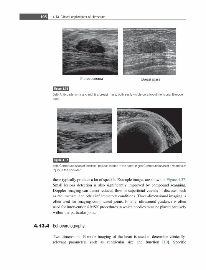
these typically produce a lot of speckle. Example images are shown in Figure 4.37.Small lesions detection is also significantly improved by compound scanning.Doppler imaging can detect reduced flow in superficial vessels in diseases suchas rheumatism, and other inflammatory conditions. Three-dimensional imaging isoften used for imaging complicated joints. Finally, ultrasound guidance is oftenused for interventional MSK procedures in which needles must be placed preciselywithin the particular joint.
4.13.4 Echocardiography
Two-dimensional B-mode imaging of the heart is used to determine clinically-relevant parameters such as ventricular size and function [10]. Specific
Fibroadenoma Breast mass
Figure 4.36
(left) A fibroadenoma and (right) a breast mass, both easily visible on a two-dimensional B-modescan.
Figure 4.37
(left) Compound scan of the flexor pollicus tendon in the hand. (right) Compound scan of a rotator cuffinjury in the shoulder.
195 4.13 Clinical applications of ultrasound
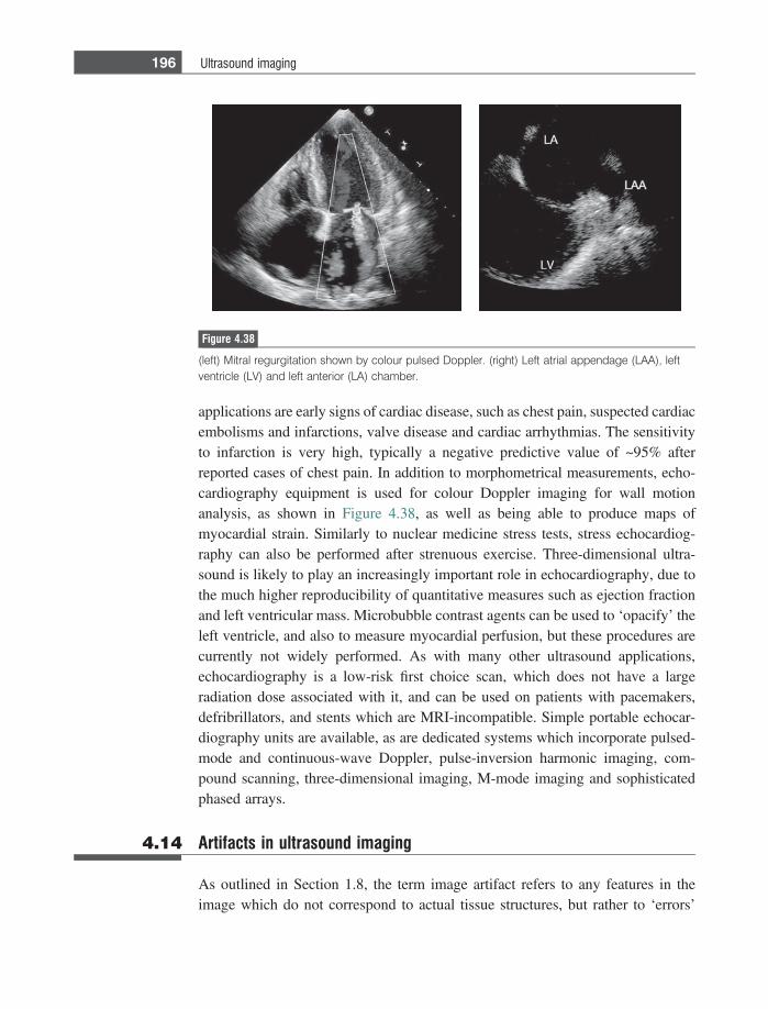
applications are early signs of cardiac disease, such as chest pain, suspected cardiacembolisms and infarctions, valve disease and cardiac arrhythmias. The sensitivityto infarction is very high, typically a negative predictive value of ~95% afterreported cases of chest pain. In addition to morphometrical measurements, echo-cardiography equipment is used for colour Doppler imaging for wall motionanalysis, as shown in Figure 4.38, as well as being able to produce maps ofmyocardial strain. Similarly to nuclear medicine stress tests, stress echocardiog-raphy can also be performed after strenuous exercise. Three-dimensional ultra-sound is likely to play an increasingly important role in echocardiography, due tothe much higher reproducibility of quantitative measures such as ejection fractionand left ventricular mass. Microbubble contrast agents can be used to ‘opacify’ theleft ventricle, and also to measure myocardial perfusion, but these procedures arecurrently not widely performed. As with many other ultrasound applications,echocardiography is a low-risk first choice scan, which does not have a largeradiation dose associated with it, and can be used on patients with pacemakers,defribrillators, and stents which are MRI-incompatible. Simple portable echocar-diography units are available, as are dedicated systems which incorporate pulsed-mode and continuous-wave Doppler, pulse-inversion harmonic imaging, com-pound scanning, three-dimensional imaging, M-mode imaging and sophisticatedphased arrays.
4.14 Artifacts in ultrasound imaging
As outlined in Section 1.8, the term image artifact refers to any features in theimage which do not correspond to actual tissue structures, but rather to ‘errors’
Figure 4.38
(left) Mitral regurgitation shown by colour pulsed Doppler. (right) Left atrial appendage (LAA), leftventricle (LV) and left anterior (LA) chamber.
196 Ultrasound imaging
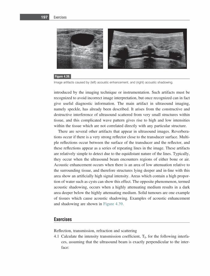
introduced by the imaging technique or instrumentation. Such artifacts must berecognized to avoid incorrect image interpretation, but once recognized can in factgive useful diagnostic information. The main artifact in ultrasound imaging,namely speckle, has already been described. It arises from the constructive anddestructive interference of ultrasound scattered from very small structures withintissue, and this complicated wave pattern gives rise to high and low intensitieswithin the tissue which are not correlated directly with any particular structure.
There are several other artifacts that appear in ultrasound images. Reverbera-tions occur if there is a very strong reflector close to the transducer surface. Multi-ple reflections occur between the surface of the transducer and the reflector, andthese reflections appear as a series of repeating lines in the image. These artifactsare relatively simple to detect due to the equidistant nature of the lines. Typically,they occur when the ultrasound beam encounters regions of either bone or air.Acoustic enhancement occurs when there is an area of low attenuation relative tothe surrounding tissue, and therefore structures lying deeper and in-line with thisarea show an artificially high signal intensity. Areas which contain a high propor-tion of water such as cysts can show this effect. The opposite phenomenon, termedacoustic shadowing, occurs when a highly attenuating medium results in a darkarea deeper below the highly attenuating medium. Solid tumours are one exampleof tissues which cause acoustic shadowing. Examples of acoustic enhancementand shadowing are shown in Figure 4.39.
Exercises
Reflection, transmission, refraction and scattering4.1 Calculate the intensity transmission coefficient, TI, for the following interfa-
ces, assuming that the ultrasound beam is exactly perpendicular to the inter-face:
Figure 4.39.
Image artifacts caused by (left) acoustic enhancement, and (right) acoustic shadowing.
197 Exercises

(i) muscle/kidney,(ii) air/muscle, and
(iii) bone/muscle.
Discuss briefly the implications of these values of TI for ultrasound imaging.4.2 Repeat the calculations in Exercise 4.1 with the angle of incidence of the
ultrasound beam now being 45�.4.3 Within tissue lies a strongly reflecting boundary, which backscatters 70% of
the intensity of the ultrasound beam. Given a 100 dB receiver dynamic range,and an operating frequency of 3 MHz, what is the maximum depth withintissue at which this boundary can be detected?
Absorption and attenuation of ultrasound energy4.4 Calculate the distance at which the intensity of a 1 MHz and 5 MHz ultrasound
beam will be reduced by half traveling through (a) bone, (b) air, and (c)muscle.
4.5 Explain why a very fast or very slow tissue relaxation time results in a verysmall amount of energy being lost due to absorption.
4.6 Plot the attenuation of the ultrasound beam for 1, 5 and 10 MHz at depthswithin tissue of 1 cm, 5 cm, and 10 cm. For each depth calculate the fractionaldecrease in transmitted power, and the absolute power assuming an outputpower from the transducer of 100 mW/cm2.
Single element transducers4.7 In order to improve the efficiency of a given transducer, the amount of energy
reflected by the skin directly under the transducer must be minimized. Alayer of material with an acoustic impedance Zmatching layer is placed betweenthe transducer and the skin. If the acoustic impedance of the skin is denotedby Zskin, and that of the transducer crystal ZPZT, show mathematically that thevalue of Zmatching layer which minimizes the energy of the reflected wave isgiven by:
Zmatching layer 5ffiffiffiffiffiffiffiffiffiffiffiffiffiffiffiffiffiffiZPZTZskinp
:
4.8 Given values of ZPZT and Zskin of 303105 g cm22 s21 and 1.73105 g cm22
s21, respectively, calculate what fraction of the energy from the transducer isactually transmitted into the patient.
4.9 If two matching layers are used instead of one, and the respective acousticimpedances are given by the analogues of the equation above, then calculatethe increase in efficiency in transmitting power into the patient.
4.10 Consider a transducer which has a thickness given by Equation (4.22). Amatching layer is used to maximize the energy transferred from the
198 Ultrasound imaging

transducer to the body. Show that the thickness of this matching layershould be one-quarter of the ultrasound wavelength.
4.11 Why is the thickness of the PZT element set to one-half wavelength?4.12 For a concave lens to focus a beam, should the speed of sound in the lens be
greater than or less than in tissue?4.13 How does the frequency profile of the ultrasound beam change as it passes
through tissue? How does this affect the lateral resolution?4.14 Consider a focused transducer with a radius of curvature of 10 cm and a
diameter of 4 cm. This transducer operates at a frequency of 3.5 MHz, andtransmits a pulse of duration 0.857 ls. What is the axial and lateral reso-lution at the focal point of the transducer?
4.15 If the axial and lateral resolution were to be improved by a factor of 2 fromthose calculated in Exercise 4.14, what physical or operating parameterscould be changed?
4.16 Plot the transmitted frequency spectrum of an ultrasound beam from a trans-ducer operating at a central frequency of 1.5 MHz. Assume that the trans-ducer is damped. Repeat the plot for the beam returning to the transducerafter having passed through tissue and been backscattered.
4.17 Draw the corresponding beam pattern to that shown in Figure 4.10 for atransducer operating at double the frequency. Note all of the frequency-dependent changes in the beam pattern.
Transducer arrays4.18 Show the required timing for simultaneous steering and dynamic focusing of
a phased array. For simplicity, sketch the general scheme using a smallnumber (for example five) of elements.
4.19 Sketch the corresponding delays required for dynamic beam-forming duringsignal reception.
Clinical scanning modes4.20 Use the following data to sketch the A-mode scan from Figure 4.40(a). The
amplitude axis should be on a dB scale, and the time axis in microseconds.Ignore any reflected signal from the transducer/fat interface, and assume thata signal of 0 dB enters the body. At a transducer frequency of 5 MHz, thelinear attenuation coefficient for muscle and liver is 5 dB cm21, and for fat is7 dB cm21. Relevant values of the characteristic acoustic impedance andspeed of sound can be found in Table 4.1.
4.21 Determine and sketch the A-mode scan using the same parameters as above,but with a time gain compensation of 0.8 dB ls21.
4.22 For the object shown in Figure 4.40(b), qualitatively sketch the B-modeultrasound image. Ignore speckle or scatter and only consider signals
199 Exercises
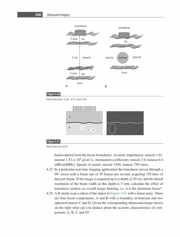
backscattered from the tissue boundaries. Acoustic impedances: muscle 1.61,tumour 1.52 (x 105 g/cm2s). Attenuation coefficients: muscle 1.0, tumour 0.4(dB/cm/MHz). Speeds of sound: muscle 1540, tumour 750 (m/s).
4.23 In a particular real-time imaging application the transducer moves through a90� sector with a frame rate of 30 frames per second, acquiring 128 lines ofdata per frame. If the image is acquired up to a depth of 20 cm, and the lateralresolution of the beam width at this depth is 5 mm, calculate the effect oftransducer motion on overall image blurring, i.e. is it the dominant factor?
4.24 A B-mode scan is taken of the object in Figure 4.41 with a linear array. Thereare four tissue components, A and B with a boundary in-between and twospherical tumors C and D. Given the corresponding ultrasound image shownon the right what can you deduce about the acoustic characteristics of com-ponents A, B, C and D?
transducer
fat
muscle
fat
liver
5 mm
5 mm
3 cm
transducer
fat
tumour musclemuscle
liver
a b
Figure 4.40
See Exercises 4.20, 4.21 and 4.22.
bd
a
c
Figure 4.41
See Exercise 4.24.
200 Ultrasound imaging
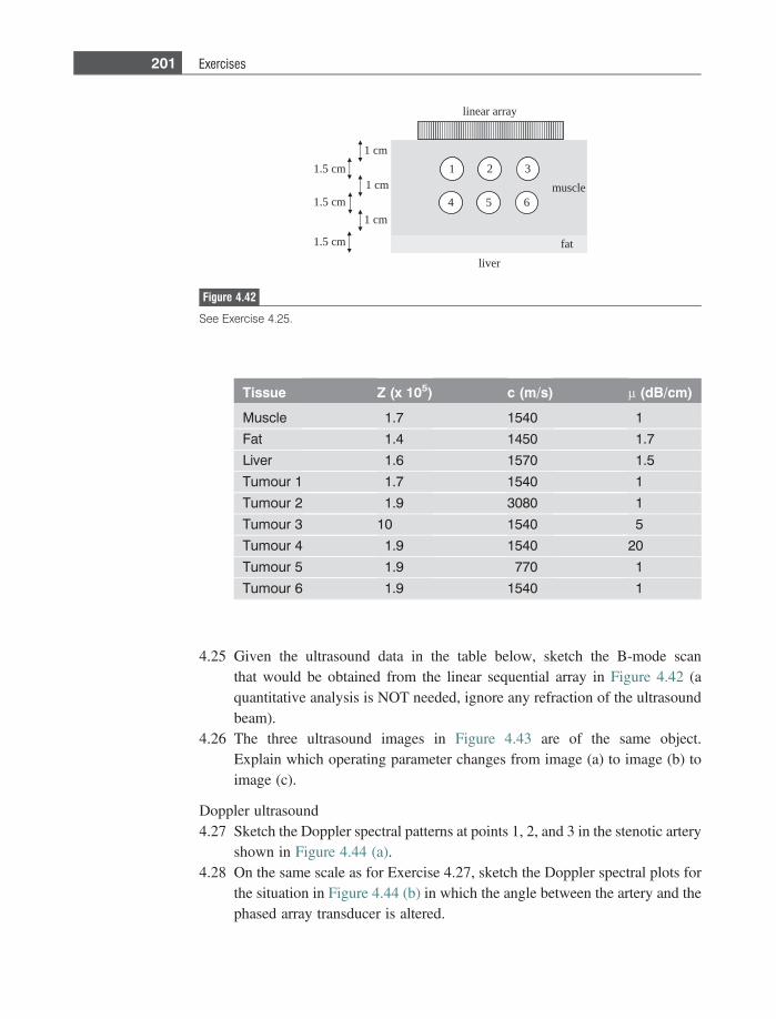
4.25 Given the ultrasound data in the table below, sketch the B-mode scanthat would be obtained from the linear sequential array in Figure 4.42 (aquantitative analysis is NOT needed, ignore any refraction of the ultrasoundbeam).
4.26 The three ultrasound images in Figure 4.43 are of the same object.Explain which operating parameter changes from image (a) to image (b) toimage (c).
Doppler ultrasound4.27 Sketch the Doppler spectral patterns at points 1, 2, and 3 in the stenotic artery
shown in Figure 4.44 (a).4.28 On the same scale as for Exercise 4.27, sketch the Doppler spectral plots for
the situation in Figure 4.44 (b) in which the angle between the artery and thephased array transducer is altered.
fat
liver
linear array
muscle
1 2 3
4 5 6
1 cm
1 cm
1 cm
1.5 cm
1.5 cm
1.5 cm
Figure 4.42
See Exercise 4.25.
Tissue Z (x 105) c (m/s) l (dB/cm)
Muscle 1.7 1540 1
Fat 1.4 1450 1.7
Liver 1.6 1570 1.5
Tumour 1 1.7 1540 1
Tumour 2 1.9 3080 1
Tumour 3 10 1540 5
Tumour 4 1.9 1540 20
Tumour 5 1.9 770 1
Tumour 6 1.9 1540 1
201 Exercises
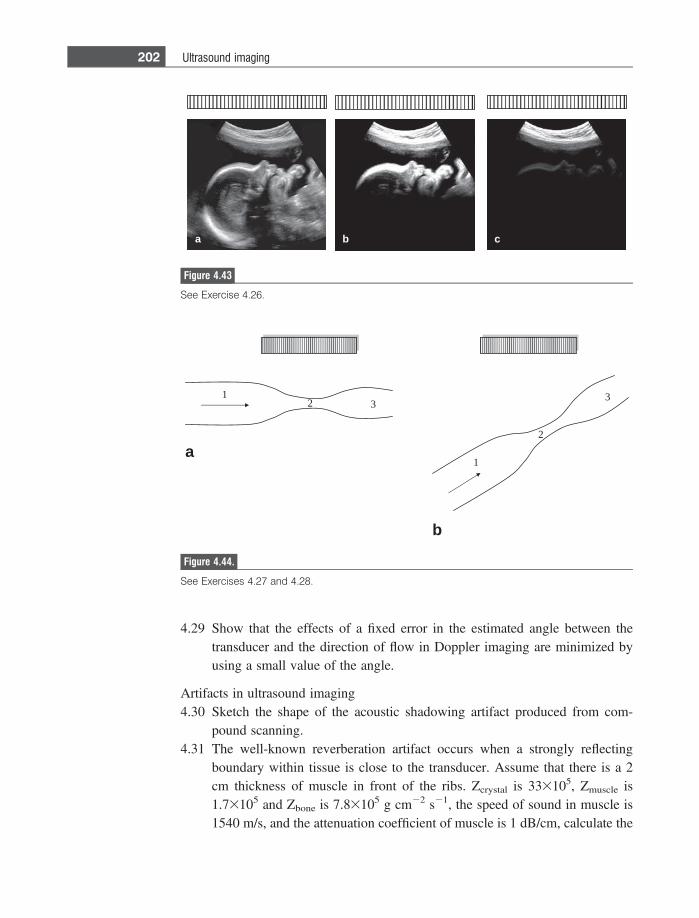
4.29 Show that the effects of a fixed error in the estimated angle between thetransducer and the direction of flow in Doppler imaging are minimized byusing a small value of the angle.
Artifacts in ultrasound imaging4.30 Sketch the shape of the acoustic shadowing artifact produced from com-
pound scanning.4.31 The well-known reverberation artifact occurs when a strongly reflecting
boundary within tissue is close to the transducer. Assume that there is a 2cm thickness of muscle in front of the ribs. Zcrystal is 333105, Zmuscle is1.73105 and Zbone is 7.83105 g cm22 s21, the speed of sound in muscle is1540 m/s, and the attenuation coefficient of muscle is 1 dB/cm, calculate the
a b c
Figure 4.43
See Exercise 4.26.
12 3
1
2
3
a
b
Figure 4.44.
See Exercises 4.27 and 4.28.
202 Ultrasound imaging

time gain compensation (units of dB/microsecond) that must be used to makethe intensity of each of the reverberation signals the same.
References
[1] Shung KK. The principle of multi-dimensional arrays. Eur J Echocardiogr 2002Jun;3(2), 149–53.
[2] Jespersen SK, Wilhjelm JE and Sillesen H. Multi-angle compound imaging.Ultrason Imaging 1998Apr;20(2), 81–102.
[3] Jensen JA. Estimation of Blood Velocities Using Ultrasound. Cambridge: CambridgeUniversity Press, 1996.
[4] Rubin JM, Bude RO, Carson PL, Bree RL and Adler RS. Power Doppler US: apotentially useful alternative to mean frequency-based color Doppler US. Radiology
1994:190(3), 853–6.[5] Stride E. Physical principles of microbubbles for ultrasound imaging and therapy.
Cerebrovasc Dis 2009;27 Suppl. 2, 1–13.[6] Kollmann C. New sonographic techniques for harmonic imaging – underlying
physical principles. Eur J Radiol 2007Nov;64(2), 164–72.[7] Barnett SB, Ter Haar GR, Ziskin MC et al. International recommendations and
guidelines for the safe use of diagnostic ultrasound in medicine. Ultrasound Med
Biol 2000;26(3), 355–66.[8] Athanasiou A, Tardivon A, Ollivier L et al. How to optimize breast ultrasound.
European Journal of Radiology 2009;69(1), 6–13.[9] Klauser AS and Peetrons P. Developments in musculoskeletal ultrasound and
clinical applications. Skeletal Radiol 2009Sep;3.[10] Marwick TH. The future of echocardiography. Eur J Echocardiogr 2009Jul;10(5),
594–601.
203 References
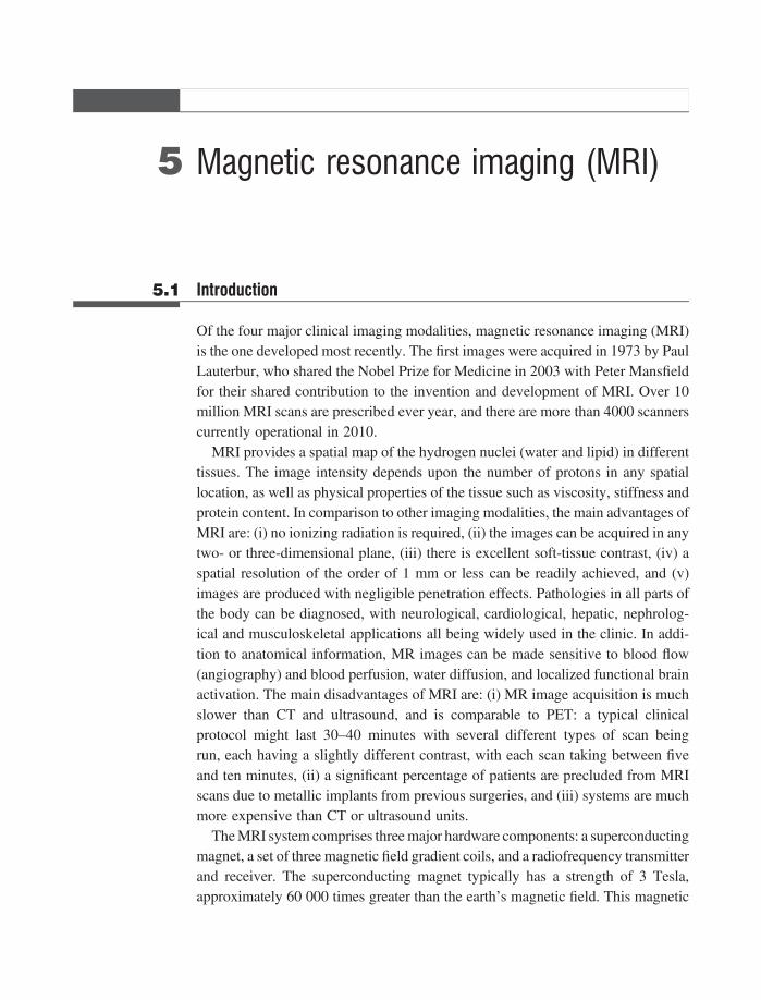
5 Magnetic resonance imaging (MRI)
5.1 Introduction
Of the four major clinical imaging modalities, magnetic resonance imaging (MRI)is the one developed most recently. The first images were acquired in 1973 by PaulLauterbur, who shared the Nobel Prize for Medicine in 2003 with Peter Mansfieldfor their shared contribution to the invention and development of MRI. Over 10million MRI scans are prescribed ever year, and there are more than 4000 scannerscurrently operational in 2010.
MRI provides a spatial map of the hydrogen nuclei (water and lipid) in differenttissues. The image intensity depends upon the number of protons in any spatiallocation, as well as physical properties of the tissue such as viscosity, stiffness andprotein content. In comparison to other imaging modalities, the main advantages ofMRI are: (i) no ionizing radiation is required, (ii) the images can be acquired in anytwo- or three-dimensional plane, (iii) there is excellent soft-tissue contrast, (iv) aspatial resolution of the order of 1 mm or less can be readily achieved, and (v)images are produced with negligible penetration effects. Pathologies in all parts ofthe body can be diagnosed, with neurological, cardiological, hepatic, nephrolog-ical and musculoskeletal applications all being widely used in the clinic. In addi-tion to anatomical information, MR images can be made sensitive to blood flow(angiography) and blood perfusion, water diffusion, and localized functional brainactivation. The main disadvantages of MRI are: (i) MR image acquisition is muchslower than CT and ultrasound, and is comparable to PET: a typical clinicalprotocol might last 30–40 minutes with several different types of scan beingrun, each having a slightly different contrast, with each scan taking between fiveand ten minutes, (ii) a significant percentage of patients are precluded from MRIscans due to metallic implants from previous surgeries, and (iii) systems are muchmore expensive than CT or ultrasound units.
The MRI system comprises three major hardware components: a superconductingmagnet, a set of three magnetic field gradient coils, and a radiofrequency transmitterand receiver. The superconducting magnet typically has a strength of 3 Tesla,approximately 60 000 times greater than the earth’s magnetic field. This magnetic
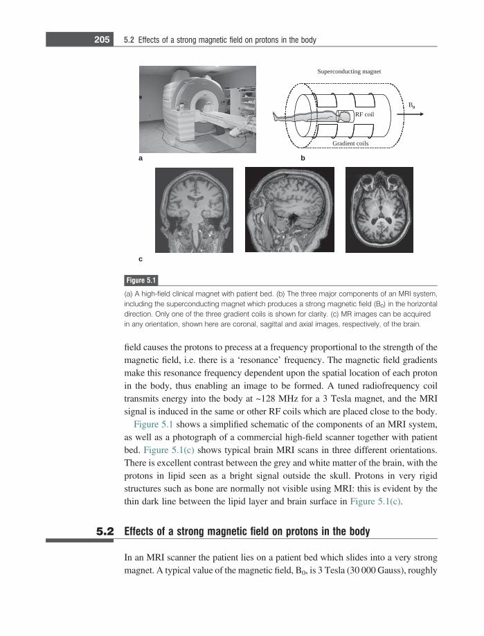
field causes the protons to precess at a frequency proportional to the strength of themagnetic field, i.e. there is a ‘resonance’ frequency. The magnetic field gradientsmake this resonance frequency dependent upon the spatial location of each protonin the body, thus enabling an image to be formed. A tuned radiofrequency coiltransmits energy into the body at ~128 MHz for a 3 Tesla magnet, and the MRIsignal is induced in the same or other RF coils which are placed close to the body.
Figure 5.1 shows a simplified schematic of the components of an MRI system,as well as a photograph of a commercial high-field scanner together with patientbed. Figure 5.1(c) shows typical brain MRI scans in three different orientations.There is excellent contrast between the grey and white matter of the brain, with theprotons in lipid seen as a bright signal outside the skull. Protons in very rigidstructures such as bone are normally not visible using MRI: this is evident by thethin dark line between the lipid layer and brain surface in Figure 5.1(c).
5.2 Effects of a strong magnetic field on protons in the body
In an MRI scanner the patient lies on a patient bed which slides into a very strongmagnet. A typical value of the magnetic field, B0, is 3 Tesla (30 000 Gauss), roughly
Superconducting magnet
Gradient coils
RF coilB0
c
0
a b
Figure 5.1
(a) A high-field clinical magnet with patient bed. (b) The three major components of an MRI system,including the superconducting magnet which produces a strong magnetic field (B0) in the horizontaldirection. Only one of the three gradient coils is shown for clarity. (c) MR images can be acquiredin any orientation, shown here are coronal, sagittal and axial images, respectively, of the brain.
205 5.2 Effects of a strong magnetic field on protons in the body
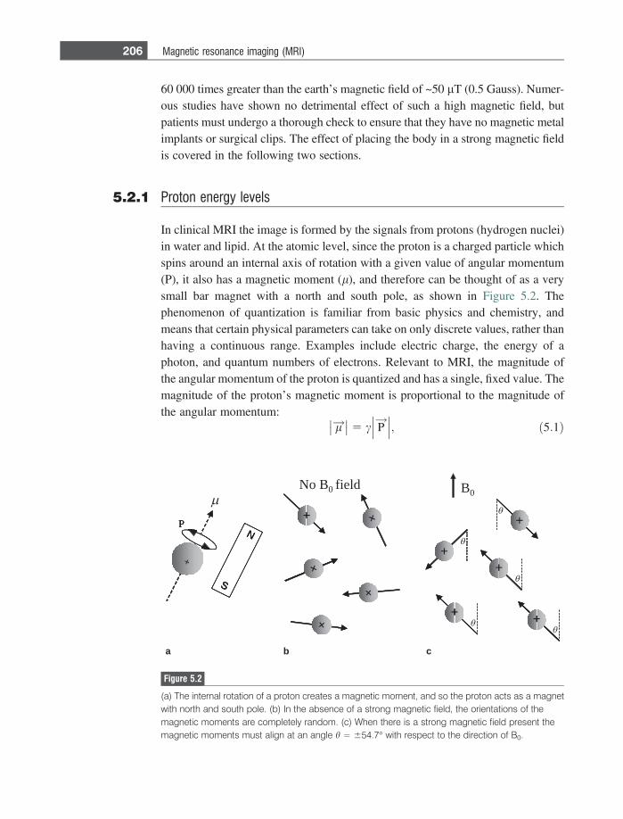
60 000 times greater than the earth’s magnetic field of ~50 lT (0.5 Gauss). Numer-ous studies have shown no detrimental effect of such a high magnetic field, butpatients must undergo a thorough check to ensure that they have no magnetic metalimplants or surgical clips. The effect of placing the body in a strong magnetic fieldis covered in the following two sections.
5.2.1 Proton energy levels
In clinical MRI the image is formed by the signals from protons (hydrogen nuclei)in water and lipid. At the atomic level, since the proton is a charged particle whichspins around an internal axis of rotation with a given value of angular momentum(P), it also has a magnetic moment (l), and therefore can be thought of as a verysmall bar magnet with a north and south pole, as shown in Figure 5.2. Thephenomenon of quantization is familiar from basic physics and chemistry, andmeans that certain physical parameters can take on only discrete values, rather thanhaving a continuous range. Examples include electric charge, the energy of aphoton, and quantum numbers of electrons. Relevant to MRI, the magnitude ofthe angular momentum of the proton is quantized and has a single, fixed value. Themagnitude of the proton’s magnetic moment is proportional to the magnitude ofthe angular momentum:
l!�� �� 5 c P
!��� ���; ð5:1Þ
+
N
S
P
No B0 field B0
+
++
+ +
++
+
+
+
a b c
+
N
S
P
++
N
S
N
S
P
++
++++
++ ++
++++
++
++
++
Figure 5.2
(a) The internal rotation of a proton creates a magnetic moment, and so the proton acts as a magnetwith north and south pole. (b) In the absence of a strong magnetic field, the orientations of themagnetic moments are completely random. (c) When there is a strong magnetic field present themagnetic moments must align at an angle h = 654.7� with respect to the direction of B0.
206 Magnetic resonance imaging (MRI)
where c is a constant called the gyromagnetic ratio, and has a value of 267.54MHz/Tesla for protons. As a result, the magnitude of the magnetic moment has asingle, fixed value. Outside the MRI magnet, as shown in Figure 5.2 the magnitudeof the magnetic moment of every proton in our bodies is fixed, but the orientationis completely random. Therefore, the net magnetization, i.e. the sum of all theindividual magnetic moments in our bodies, is zero (ignoring the very small effectsfrom the earth’s magnetic field).
The situation changes when the patient is slid into the magnet for an MRI scan.From quantum mechanics, the component of the magnetic moment in the directionof B0 can have only two discrete values, which results in the magnetic momentsbeing aligned at an angle of 54.7� with respect to the direction B0, aligned either inthe same direction or in the opposite direction, as shown in Figure 5.2(c). Theformer configuration is termed as the parallel, and the latter as the anti-parallelconfiguration: note however that the terms parallel and anti-parallel only refer tothe z-component of l, and that l is actually aligned at an angle with respect to B0.
The relative number of protons in the parallel and anti-parallel configurationsdepends upon the value of B0. Protons in the parallel configuration are in the moreenergy ‘favourable’ state, compared to the anti-parallel configuration. The energydifference (DE) between the two states is shown in Figure 5.3 and given by:
DE 5chB0
2p; ð5:2Þ
where h is Plank’s constant (6.63 3 10234 J s). To calculate the relativenumber of protons in each of the two configurations the Boltzmann equationcan be used:
Nanti-parallel
Nparallel5 exp� DE
kT
� �5 exp� chBo
2pkT
� �: ð5:3Þ
where k is Boltzmann’s constant with a value of 1.38310223 J/K, and T is thetemperature measured in Kelvin. Since the value of the exponent is very small, afirst order approximation, e2x � 12x, can be made:
Nanti-parallel
Nparallel5 1� chBo
2pkT
� �: ð5:4Þ
The MRI signal depends upon the difference in populations between the twoenergy levels:
Nparallel � Nanti-parallel 5 NtotalchB0
4pkT; ð5:5Þ
where Ntotal is the total number of protons. It is important to note that MRI candetect only the difference Nparallel2Nanti-parallel, and not the total number of protons.
207 5.2 Effects of a strong magnetic field on protons in the body
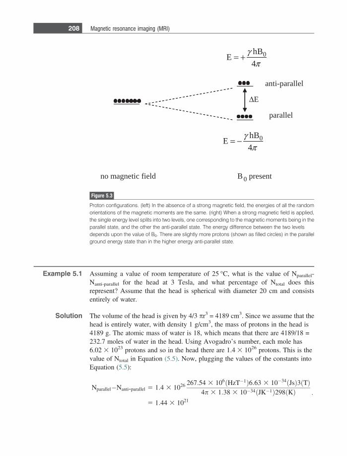
Example 5.1 Assuming a value of room temperature of 25 �C, what is the value of Nparallel-Nanti-parallel for the head at 3 Tesla, and what percentage of Ntotal does thisrepresent? Assume that the head is spherical with diameter 20 cm and consistsentirely of water.
Solution The volume of the head is given by 4/3 pr3 = 4189 cm3. Since we assume that thehead is entirely water, with density 1 g/cm3, the mass of protons in the head is4189 g. The atomic mass of water is 18, which means that there are 4189/18 =232.7 moles of water in the head. Using Avogadro’s number, each mole has6.02 3 1023 protons and so in the head there are 1.4 3 1026 protons. This is thevalue of Ntotal in Equation (5.5). Now, plugging the values of the constants intoEquation (5.5):
Nparallel�Nanti-parallel 5 1:4 3 1026 267:54 3 106 HzT�1ð Þ6:63 3 10�34ðJsÞ3 Tð Þ4p 3 1:38 3 10�34 JK�1ð Þ298 Kð Þ
5 1:44 3 1021
:
no magnetic field B 0 present
parallel
anti-parallel
0hBE
4= +
0hBE
4= −
ΔE
Figure 5.3
Proton configurations. (left) In the absence of a strong magnetic field, the energies of all the randomorientations of the magnetic moments are the same. (right) When a strong magnetic field is applied,the single energy level splits into two levels, one corresponding to the magnetic moments being in theparallel state, and the other the anti-parallel state. The energy difference between the two levelsdepends upon the value of B0. There are slightly more protons (shown as filled circles) in the parallelground energy state than in the higher energy anti-parallel state.
208 Magnetic resonance imaging (MRI)
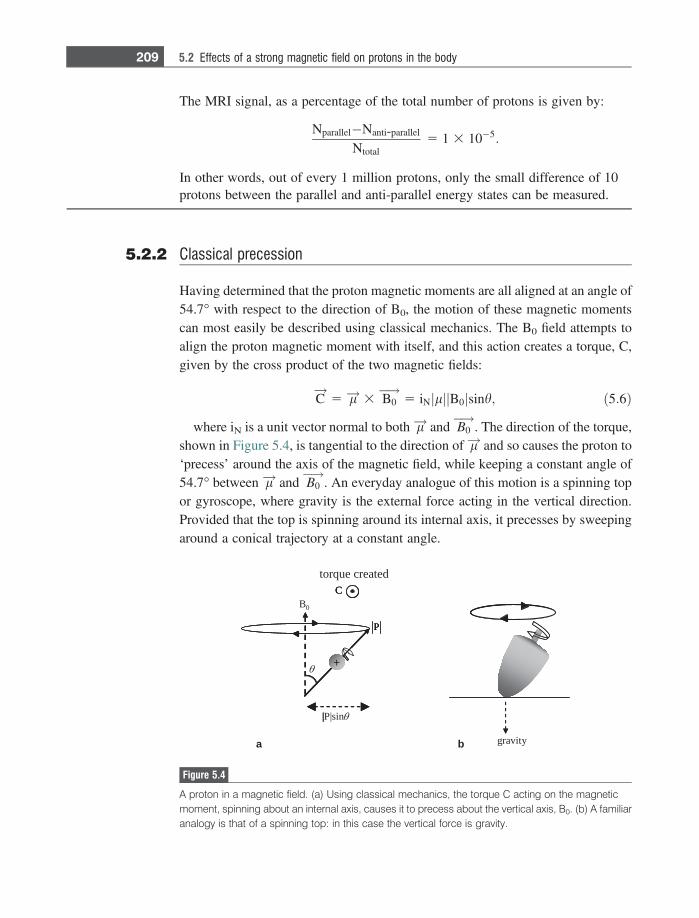
The MRI signal, as a percentage of the total number of protons is given by:
Nparallel�Nanti-parallel
Ntotal5 1 3 10�5:
In other words, out of every 1 million protons, only the small difference of 10protons between the parallel and anti-parallel energy states can be measured.
5.2.2 Classical precession
Having determined that the proton magnetic moments are all aligned at an angle of54.7� with respect to the direction of B0, the motion of these magnetic momentscan most easily be described using classical mechanics. The B0 field attempts toalign the proton magnetic moment with itself, and this action creates a torque, C,given by the cross product of the two magnetic fields:
C!
5 l!3 B0 !
5 iN lj j B0j jsinh; ð5:6Þ
where iN is a unit vector normal to both l! and B0 !
. The direction of the torque,shown in Figure 5.4, is tangential to the direction of l! and so causes the proton to‘precess’ around the axis of the magnetic field, while keeping a constant angle of54.7� between l! and B0
!. An everyday analogue of this motion is a spinning top
or gyroscope, where gravity is the external force acting in the vertical direction.Provided that the top is spinning around its internal axis, it precesses by sweepingaround a conical trajectory at a constant angle.
gravity
B0
θ
|P|sinθ
C
P
+
torque created
a b
|
C
P
+
|
C
P
+
Figure 5.4
A proton in a magnetic field. (a) Using classical mechanics, the torque C acting on the magneticmoment, spinning about an internal axis, causes it to precess about the vertical axis, B0. (b) A familiaranalogy is that of a spinning top: in this case the vertical force is gravity.
209 5.2 Effects of a strong magnetic field on protons in the body
To calculate how fast a proton precesses, we use the fact that the torque isdefined as the time rate of change of the proton’s angular momentum:
C!
5d P!
dt5 l!3 B0
!: ð5:7Þ
From Figure 5.4, the magnitude of the component of the angular momentumwhich precesses in the plane perpendicular to B0 is given by P
!��� ��� sinh. In ashort time dt, l precesses through an angle du resulting in a change d P
!in the
angular momentum. Simple trigonometry gives the relationship that:
sin duð Þ 5d P!
P!��� ���sinh
5C!
dt
P!��� ���sinh
: ð5:8Þ
If du is small then we can make the approximation that sin(du) = du. Theangular precession frequency, x, is given by du/dt and so has a value:
x 5dudt
5C!
P!��� ��� sinh
5l!3 B0
!P!��� ��� sinh
5c P!
3 B0 !
P!��� ��� sinh
5c P!��� ��� B0
!��� ��� sinh
P!��� ��� sinh
5 cB0:
ð5:9Þ
The effect of placing a proton in a magnetic field, therefore, is to cause it toprecess around B0 at a frequency directly proportional to the strength of themagnetic field. This frequency, termed x0, is termed the Larmor frequency afterthe renowned Irish physicist Joseph Larmor.
Example 5.2 What are the Larmor frequencies, expressed in MHz, for B0 fields of 1.5 Tesla,3 Tesla and 7 Tesla?
Solution For 1.5 Tesla, the frequency is given by:
f 5x2p
5cB0
2p5
267:54 3 106 HzT�1ð Þ1:5 Tð Þ2p
5 63:9 MHz:
Simple multiplication gives frequencies (rounded to one significant figure) of127.7 and 298.1 MHz for 3 Tesla and 7 Tesla, respectively.
By combining the results of the quantum mechanical and classical analysis wecan represent the net magnetization from the entire patient in a simple vector form.Figure 5.5 shows on the left a representation of several proton magnetic moments,
210 Magnetic resonance imaging (MRI)
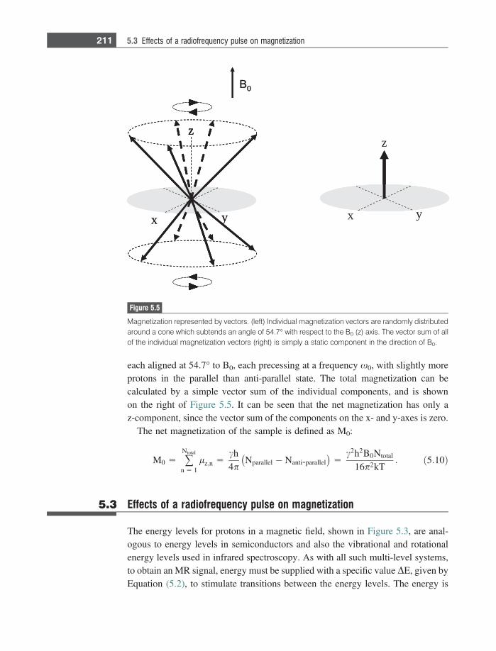
each aligned at 54.7� to B0, each precessing at a frequency x0, with slightly moreprotons in the parallel than anti-parallel state. The total magnetization can becalculated by a simple vector sum of the individual components, and is shownon the right of Figure 5.5. It can be seen that the net magnetization has only az-component, since the vector sum of the components on the x- and y-axes is zero.
The net magnetization of the sample is defined as M0:
M0 5 +Ntotal
n 5 1lz;n 5
ch4p
Nparallel � Nanti-parallel� �
5c2h2B0Ntotal
16p2kT: ð5:10Þ
5.3 Effects of a radiofrequency pulse on magnetization
The energy levels for protons in a magnetic field, shown in Figure 5.3, are anal-ogous to energy levels in semiconductors and also the vibrational and rotationalenergy levels used in infrared spectroscopy. As with all such multi-level systems,to obtain an MR signal, energy must be supplied with a specific value DE, given byEquation (5.2), to stimulate transitions between the energy levels. The energy is
x y
z
B 0
x y
z
x y
zz
B 0
Figure 5.5
Magnetization represented by vectors. (left) Individual magnetization vectors are randomly distributedaround a cone which subtends an angle of 54.7� with respect to the B0 (z) axis. The vector sum of allof the individual magnetization vectors (right) is simply a static component in the direction of B0.
211 5.3 Effects of a radiofrequency pulse on magnetization

supplied as an electromagnetic (EM), usually referred to as a radiofrequency (RF)field, the frequency (f) of which can be calculated from De Broglie’s relationship,DE=hf:
hf 5 DE 5chB0
2p
0f 5cB0
2por x 5 cB0
: ð5:11Þ
By comparing Equations (5.11) and (5.9) it can be seen that the frequency of theRF field is identical to the precession frequency.
5.3.1 Creation of transverse magnetization
In MRI, energy is applied as a short RF pulse, with the direction of the magneticcomponent of the RF field oriented at 90� to the direction of B0, as shown in Figure5.6. Applying the same classical analysis as for proton precession, the magneticcomponent of the RF pulse, termed the B1 field, produces a torque which causesthe net magnetization to rotate towards the xy-plane as shown in Figure 5.6. Notethat if the B1 field is applied along the x-axis, the magnetic moment vector isrotated towards the y-axis (see Exercise 5.2).
The ‘tip angle’ (a) is defined as the angle through which the net magnetization isrotated. This angle is proportional to both the strength of the applied RF field(measured in Tesla) and the time, sB1, for which it is applied:
a 5 cB1sB1: ð5:12Þ
A tip angle of 90�, termed a 90� pulse, results in the maximum value of the My
component of magnetization, whereas one of 180� produces no My magnetizationbut rotates the net magnetization M0 from the +z to the – z axis.
B1
x y
z
0x y
z
B11
0y
z
00
Figure 5.6
(left) Application of an RF pulse about the x-axis rotates the magnetization from the z-direction towardsthe y-axis. If the RF pulse strength and duration are chosen to produce a 90� pulse, then themagnetization lies directly along the y-axis. When the RF pulse is switched off (right), themagnetization precesses around the z-axis at the Larmor frequency x0.
212 Magnetic resonance imaging (MRI)
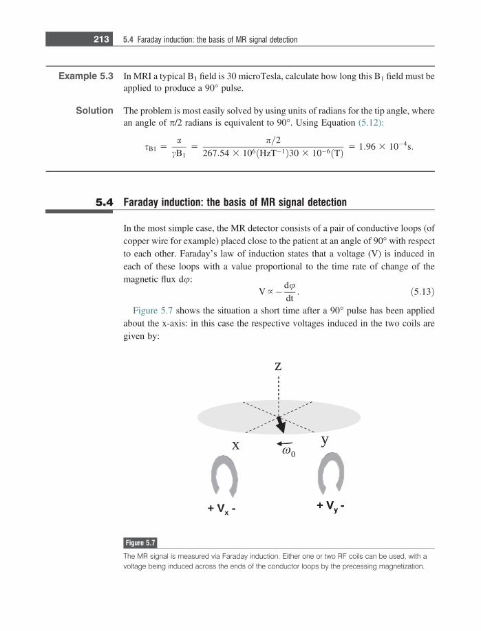
Example 5.3 In MRI a typical B1 field is 30 microTesla, calculate how long this B1 field must beapplied to produce a 90� pulse.
Solution The problem is most easily solved by using units of radians for the tip angle, wherean angle of p/2 radians is equivalent to 90�. Using Equation (5.12):
sB1 5a
cB15
p=2267:54 3 106 HzT�1ð Þ30 3 10�6 Tð Þ 5 1:96 3 10�4s:
5.4 Faraday induction: the basis of MR signal detection
In the most simple case, the MR detector consists of a pair of conductive loops (ofcopper wire for example) placed close to the patient at an angle of 90� with respectto each other. Faraday’s law of induction states that a voltage (V) is induced ineach of these loops with a value proportional to the time rate of change of themagnetic flux du:
V }� dudt: ð5:13Þ
Figure 5.7 shows the situation a short time after a 90� pulse has been appliedabout the x-axis: in this case the respective voltages induced in the two coils aregiven by:
0
+ Vx
-
x y
z
+ Vy
-Vx
- + Vy
-
Figure 5.7
The MR signal is measured via Faraday induction. Either one or two RF coils can be used, with avoltage being induced across the ends of the conductor loops by the precessing magnetization.
213 5.4 Faraday induction: the basis of MR signal detection
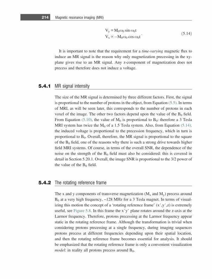
Vy } M0x0 sin x0t
Vx }�M0x0 cos x0t: ð5:14Þ
It is important to note that the requirement for a time-varying magnetic flux toinduce an MR signal is the reason why only magnetization precessing in the xy-plane gives rise to an MR signal. Any z-component of magnetization does notprecess and therefore does not induce a voltage.
5.4.1 MR signal intensity
The size of the MR signal is determined by three different factors. First, the signalis proportional to the number of protons in the object, from Equation (5.5). In termsof MRI, as will be seen later, this corresponds to the number of protons in eachvoxel of the image. The other two factors depend upon the value of the B0 field.From Equation (5.10), the value of M0 is proportional to B0: therefore a 3 TeslaMRI system has twice the M0 of a 1.5 Tesla system. Also, from Equation (5.14),the induced voltage is proportional to the precession frequency, which in turn isproportional to B0. Overall, therefore, the MR signal is proportional to the squareof the B0 field, one of the reasons why there is such a strong drive towards higherfield MRI systems. Of course, in terms of the overall SNR, the dependence of thenoise on the strength of the B0 field must also be considered: this is covered indetail in Section 5.20.1. Overall, the image SNR is proportional to the 3/2 power ofthe value of the B0 field.
5.4.2 The rotating reference frame
The x and y components of transverse magnetization (Mx and My) precess aroundB0 at a very high frequency, ~128 MHz for a 3 Tesla magnet. In terms of visual-izing this motion the concept of a ‘rotating reference frame’ (x#,y#,z) is extremelyuseful, see Figure 5.8. In this frame the x#y# plane rotates around the z-axis at theLarmor frequency. Therefore, protons precessing at the Larmor frequency appearstatic in the rotating reference frame. Although the transformation is trivial whenconsidering protons precessing at a single frequency, during imaging sequencesprotons precess at different frequencies depending upon their spatial location,and then the rotating reference frame becomes essential for analysis. It shouldbe emphasized that the rotating reference frame is only a convenient visualizationmodel: in reality all protons precess around B0.
214 Magnetic resonance imaging (MRI)
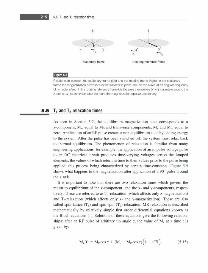
5.5 T1 and T2 relaxation times
As seen in Section 5.2, the equilibrium magnetization state corresponds to az-component, Mz, equal to M0 and transverse components, Mx and My, equal tozero. Application of an RF pulse creates a non-equilibrium state by adding energyto the system. After the pulse has been switched off, the system must relax backto thermal equilibrium. The phenomenon of relaxation is familiar from manyengineering applications: for example, the application of an impulse voltage pulseto an RC electrical circuit produces time-varying voltages across the lumpedelements, the values of which return in time to their values prior to the pulse beingapplied, this process being characterized by certain time-constants. Figure 5.9shows what happens to the magnetization after application of a 90� pulse aroundthe x axis.
It is important to note that there are two relaxation times which govern thereturn to equilibrium of the z-component, and the x- and y-components, respec-tively. These are referred to as T1-relaxation (which affects only z-magnetization)and T2-relaxation (which affects only x- and y-magnetization). These are alsocalled spin-lattice (T1) and spin-spin (T2) relaxation. MR relaxation is describedmathematically by relatively simple first order differential equations known asthe Bloch equations [1]. Solutions of these equations give the following relation-ships: after an RF pulse of arbitrary tip angle a, the value of Mz at a time t isgiven by:
MzðtÞ 5 M0 cos a 1 M0 �M0 cos að Þ 1� e�t
T1
� �: ð5:15Þ
' x ' y
z
x y
z
Stationary frame Rotating reference frame
0 0
0
Figure 5.8
Relationship between the stationary frame (left) and the rotating frame (right). In the stationaryframe the magnetization precesses in the transverse plane around the z-axis at an angular frequencyof x0 radians/sec. In the rotating reference frame it is the axes themselves (x#,y#) that rotate around thez-axis at x0 radians/sec, and therefore the magnetization appears stationary.
215 5.5 T1 and T2 relaxation times
For example, after a 90� pulse the value of Mz is given by:
MzðtÞ 5 M0 1� e�t
T1
� �: ð5:16Þ
Different tissues have different values of T1, and diseased tissues often havesubstantially altered T1 relaxation time compared to healthy tissue, and thesedifferences form one basis for introducing contrast into the MR image. Valuesof tissue T1 values for 1.5 and 3 Tesla are shown in Table 5.1. It can be seen thatthe values of T1 depend not only upon tissue type but also the magnetic fieldstrength, a topic covered more fully in Section 5.13.
Figure 5.10 shows the time dependence of the Mz magnetization after a 90�pulse for two tissues with different T1 values.
The second relaxation time, T2, governs the return of the Mx and My compo-nents of magnetization to their thermal equilibrium values of zero. If an RF pulseof arbitrary tip angle a is applied along the x-axis, the value of My at time t after theRF pulse is given by:
MyðtÞ 5 M0 sin a exp� tT2
� �: ð5:17Þ
As is the case for T1 relaxation times, different tissues in the body have differentvalues of T2, and these can also be used to differentiate between healthy anddiseased tissues in clinical images. Similarly to T1, the values of T2 also dependon B0, and Table 5.1 shows typical values at 1.5 and 3 Tesla. It should be noted thatthere is no direct correlation between the T1 and T2 values, a long T1 does notnecessarily mean a long T2. The only thing that is universally true, detailed furtherin Section 5.13, is that T1 is always greater than T2.
'y'x
z
'y'x
z
'y'x
z
time
Figure 5.9
(left) Magnetization vector after a 90� RF pulse about the x-axis. (centre) T1 and T2 relaxation of themagnetization a certain time after the pulse has been applied results in an increased Mz componentand reduced My component, respectively. (right) After a further time, the Mz and My componentshave almost returned to their equilibrium values of M0 and zero, respectively.
216 Magnetic resonance imaging (MRI)
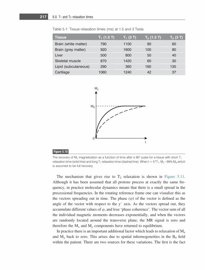
The mechanism that gives rise to T2 relaxation is shown in Figure 5.11.Although it has been assumed that all protons precess at exactly the same fre-quency, in practice molecular dynamics means that there is a small spread in theprecessional frequencies. In the rotating reference frame one can visualize this asthe vectors spreading out in time. The phase (u) of the vector is defined as theangle of the vector with respect to the y# axis. As the vectors spread out, theyaccumulate different values of u, and lose ‘phase coherence’. The vector sum of allthe individual magnetic moments decreases exponentially, and when the vectorsare randomly located around the transverse plane, the MR signal is zero andtherefore the Mx and My components have returned to equilibrium.
In practice there is an important additional factor which leads to relaxation of Mx
and My back to zero. This arises due to spatial inhomogeneities in the B0 fieldwithin the patient. There are two sources for these variations. The first is the fact
t
Mz
M0
0
Figure 5.10
The recovery of Mz magnetization as a function of time after a 90� pulse for a tissue with short T1
relaxation time (solid line) and long T1 relaxation time (dashed line). When t = 5*T1, Mz~99% M0,whichis assumed to be full recovery.
Table 5.1: Tissue relaxation times (ms) at 1.5 and 3 Tesla
Tissue T1 (1.5 T) T1 (3 T) T2 (1.5 T) T2 (3 T)
Brain (white matter) 790 1100 90 60
Brain (grey matter) 920 1600 100 80
Liver 500 800 50 40
Skeletal muscle 870 1420 60 30
Lipid (subcutaneous) 290 360 160 130
Cartilage 1060 1240 42 37
217 5.5 T1 and T2 relaxation times
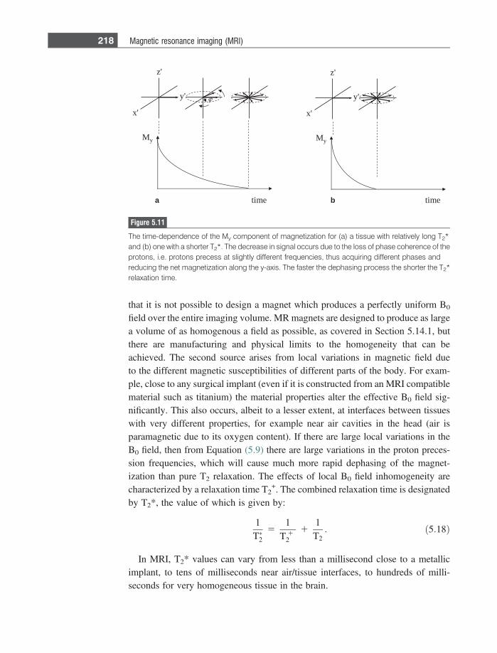
that it is not possible to design a magnet which produces a perfectly uniform B0
field over the entire imaging volume. MR magnets are designed to produce as largea volume of as homogenous a field as possible, as covered in Section 5.14.1, butthere are manufacturing and physical limits to the homogeneity that can beachieved. The second source arises from local variations in magnetic field dueto the different magnetic susceptibilities of different parts of the body. For exam-ple, close to any surgical implant (even if it is constructed from an MRI compatiblematerial such as titanium) the material properties alter the effective B0 field sig-nificantly. This also occurs, albeit to a lesser extent, at interfaces between tissueswith very different properties, for example near air cavities in the head (air isparamagnetic due to its oxygen content). If there are large local variations in theB0 field, then from Equation (5.9) there are large variations in the proton preces-sion frequencies, which will cause much more rapid dephasing of the magnet-ization than pure T2 relaxation. The effects of local B0 field inhomogeneity arecharacterized by a relaxation time T2
+. The combined relaxation time is designatedby T2*, the value of which is given by:
1T�2
51
T 12
11T2: ð5:18Þ
In MRI, T2* values can vary from less than a millisecond close to a metallicimplant, to tens of milliseconds near air/tissue interfaces, to hundreds of milli-seconds for very homogeneous tissue in the brain.
My
'x
'y
'z
My
'x
'y
'z
timetimea b
Figure 5.11
The time-dependence of the My component of magnetization for (a) a tissue with relatively long T2*and (b) one with a shorter T2*. The decrease in signal occurs due to the loss of phase coherence of theprotons, i.e. protons precess at slightly different frequencies, thus acquiring different phases andreducing the net magnetization along the y-axis. The faster the dephasing process the shorter the T2*relaxation time.
218 Magnetic resonance imaging (MRI)
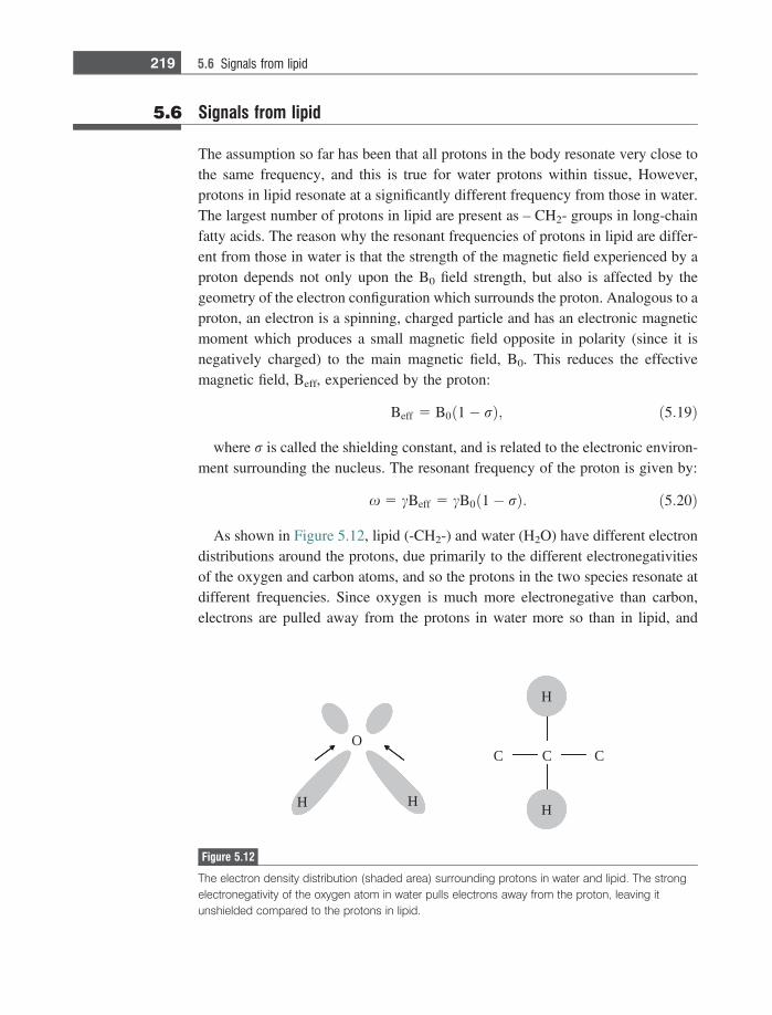
5.6 Signals from lipid
The assumption so far has been that all protons in the body resonate very close tothe same frequency, and this is true for water protons within tissue, However,protons in lipid resonate at a significantly different frequency from those in water.The largest number of protons in lipid are present as – CH2- groups in long-chainfatty acids. The reason why the resonant frequencies of protons in lipid are differ-ent from those in water is that the strength of the magnetic field experienced by aproton depends not only upon the B0 field strength, but also is affected by thegeometry of the electron configuration which surrounds the proton. Analogous to aproton, an electron is a spinning, charged particle and has an electronic magneticmoment which produces a small magnetic field opposite in polarity (since it isnegatively charged) to the main magnetic field, B0. This reduces the effectivemagnetic field, Beff, experienced by the proton:
Beff 5 B0ð1� rÞ; ð5:19Þ
where r is called the shielding constant, and is related to the electronic environ-ment surrounding the nucleus. The resonant frequency of the proton is given by:
x 5 cBeff 5 cB0ð1� rÞ: ð5:20Þ
As shown in Figure 5.12, lipid (-CH2-) and water (H2O) have different electrondistributions around the protons, due primarily to the different electronegativitiesof the oxygen and carbon atoms, and so the protons in the two species resonate atdifferent frequencies. Since oxygen is much more electronegative than carbon,electrons are pulled away from the protons in water more so than in lipid, and
O
H H
C CC
H
H
Figure 5.12
The electron density distribution (shaded area) surrounding protons in water and lipid. The strongelectronegativity of the oxygen atom in water pulls electrons away from the proton, leaving itunshielded compared to the protons in lipid.
219 5.6 Signals from lipid
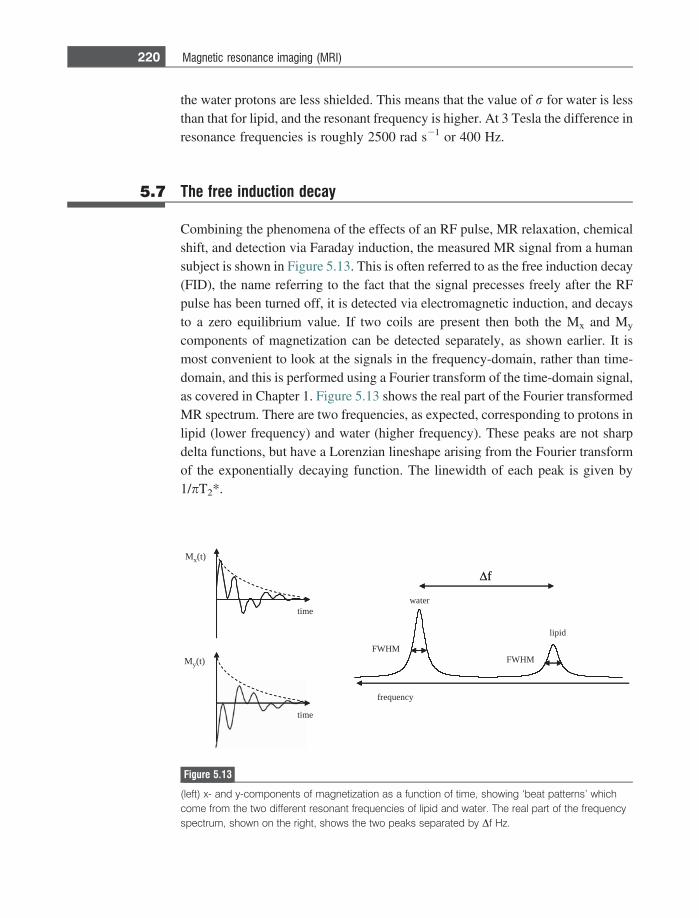
the water protons are less shielded. This means that the value of r for water is lessthan that for lipid, and the resonant frequency is higher. At 3 Tesla the difference inresonance frequencies is roughly 2500 rad s21 or 400 Hz.
5.7 The free induction decay
Combining the phenomena of the effects of an RF pulse, MR relaxation, chemicalshift, and detection via Faraday induction, the measured MR signal from a humansubject is shown in Figure 5.13. This is often referred to as the free induction decay(FID), the name referring to the fact that the signal precesses freely after the RFpulse has been turned off, it is detected via electromagnetic induction, and decaysto a zero equilibrium value. If two coils are present then both the Mx and My
components of magnetization can be detected separately, as shown earlier. It ismost convenient to look at the signals in the frequency-domain, rather than time-domain, and this is performed using a Fourier transform of the time-domain signal,as covered in Chapter 1. Figure 5.13 shows the real part of the Fourier transformedMR spectrum. There are two frequencies, as expected, corresponding to protons inlipid (lower frequency) and water (higher frequency). These peaks are not sharpdelta functions, but have a Lorenzian lineshape arising from the Fourier transformof the exponentially decaying function. The linewidth of each peak is given by1/pT2*.
time
time
frequency
water
lipid
Δ f
FWHMFWHM
Mx(t)
My(t)
Δ f
Figure 5.13
(left) x- and y-components of magnetization as a function of time, showing ‘beat patterns’ whichcome from the two different resonant frequencies of lipid and water. The real part of the frequencyspectrum, shown on the right, shows the two peaks separated by Df Hz.
220 Magnetic resonance imaging (MRI)
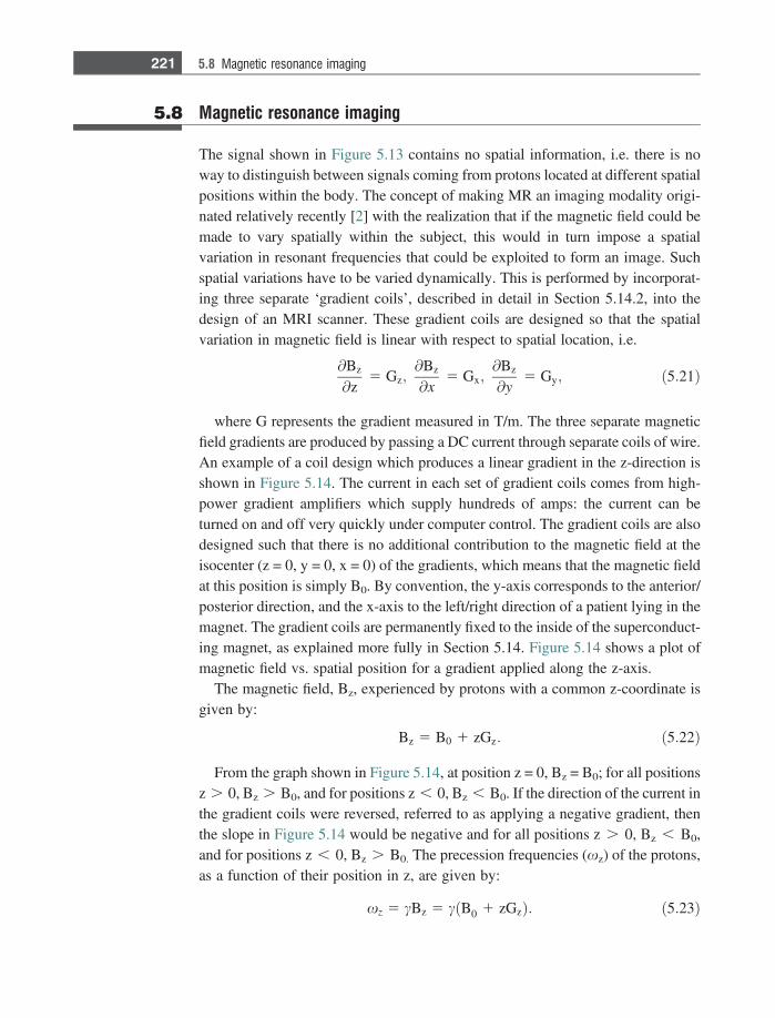
5.8 Magnetic resonance imaging
The signal shown in Figure 5.13 contains no spatial information, i.e. there is noway to distinguish between signals coming from protons located at different spatialpositions within the body. The concept of making MR an imaging modality origi-nated relatively recently [2] with the realization that if the magnetic field could bemade to vary spatially within the subject, this would in turn impose a spatialvariation in resonant frequencies that could be exploited to form an image. Suchspatial variations have to be varied dynamically. This is performed by incorporat-ing three separate ‘gradient coils’, described in detail in Section 5.14.2, into thedesign of an MRI scanner. These gradient coils are designed so that the spatialvariation in magnetic field is linear with respect to spatial location, i.e.
@Bz
@z5 Gz;
@Bz
@x5 Gx;
@Bz
@y5 Gy; ð5:21Þ
where G represents the gradient measured in T/m. The three separate magneticfield gradients are produced by passing a DC current through separate coils of wire.An example of a coil design which produces a linear gradient in the z-direction isshown in Figure 5.14. The current in each set of gradient coils comes from high-power gradient amplifiers which supply hundreds of amps: the current can beturned on and off very quickly under computer control. The gradient coils are alsodesigned such that there is no additional contribution to the magnetic field at theisocenter (z = 0, y = 0, x = 0) of the gradients, which means that the magnetic fieldat this position is simply B0. By convention, the y-axis corresponds to the anterior/posterior direction, and the x-axis to the left/right direction of a patient lying in themagnet. The gradient coils are permanently fixed to the inside of the superconduct-ing magnet, as explained more fully in Section 5.14. Figure 5.14 shows a plot ofmagnetic field vs. spatial position for a gradient applied along the z-axis.
The magnetic field, Bz, experienced by protons with a common z-coordinate isgiven by:
Bz 5 B0 1 zGz: ð5:22Þ
From the graph shown in Figure 5.14, at position z = 0, Bz = B0; for all positionsz . 0, Bz . B0, and for positions z , 0, Bz , B0. If the direction of the current inthe gradient coils were reversed, referred to as applying a negative gradient, thenthe slope in Figure 5.14 would be negative and for all positions z . 0, Bz , B0,and for positions z , 0, Bz . B0. The precession frequencies (xz) of the protons,as a function of their position in z, are given by:
xz 5 cBz 5 cðB0 1 zGzÞ: ð5:23Þ
221 5.8 Magnetic resonance imaging
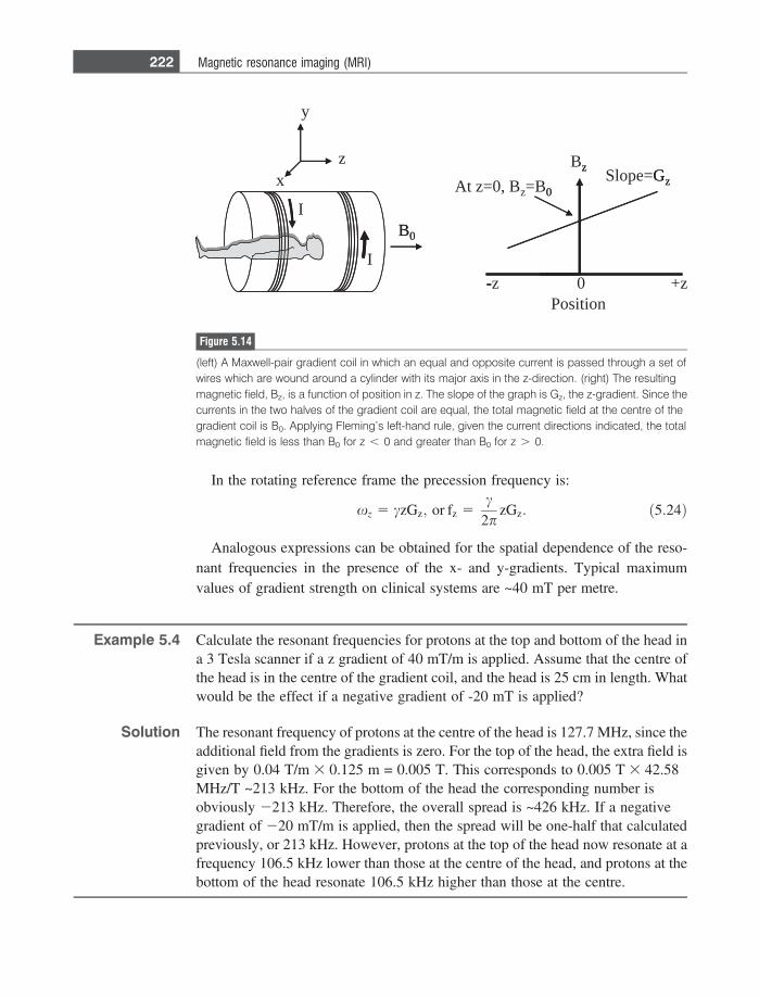
In the rotating reference frame the precession frequency is:
xz 5 czGz; or fz 5c
2pzGz: ð5:24Þ
Analogous expressions can be obtained for the spatial dependence of the reso-nant frequencies in the presence of the x- and y-gradients. Typical maximumvalues of gradient strength on clinical systems are ~40 mT per metre.
Example 5.4 Calculate the resonant frequencies for protons at the top and bottom of the head ina 3 Tesla scanner if a z gradient of 40 mT/m is applied. Assume that the centre ofthe head is in the centre of the gradient coil, and the head is 25 cm in length. Whatwould be the effect if a negative gradient of -20 mT is applied?
Solution The resonant frequency of protons at the centre of the head is 127.7 MHz, since theadditional field from the gradients is zero. For the top of the head, the extra field isgiven by 0.04 T/m 3 0.125 m = 0.005 T. This corresponds to 0.005 T 3 42.58MHz/T ~213 kHz. For the bottom of the head the corresponding number isobviously 2213 kHz. Therefore, the overall spread is ~426 kHz. If a negativegradient of 220 mT/m is applied, then the spread will be one-half that calculatedpreviously, or 213 kHz. However, protons at the top of the head now resonate at afrequency 106.5 kHz lower than those at the centre of the head, and protons at thebottom of the head resonate 106.5 kHz higher than those at the centre.
B0
x
y
z
Position
At z=0, Bz=B0
+z-z
Slope=GzBz
0
I
I
B0
0
-
Gzz
Figure 5.14
(left) A Maxwell-pair gradient coil in which an equal and opposite current is passed through a set ofwires which are wound around a cylinder with its major axis in the z-direction. (right) The resultingmagnetic field, Bz, is a function of position in z. The slope of the graph is Gz, the z-gradient. Since thecurrents in the two halves of the gradient coil are equal, the total magnetic field at the centre of thegradient coil is B0. Applying Fleming’s left-hand rule, given the current directions indicated, the totalmagnetic field is less than B0 for z , 0 and greater than B0 for z . 0.
222 Magnetic resonance imaging (MRI)
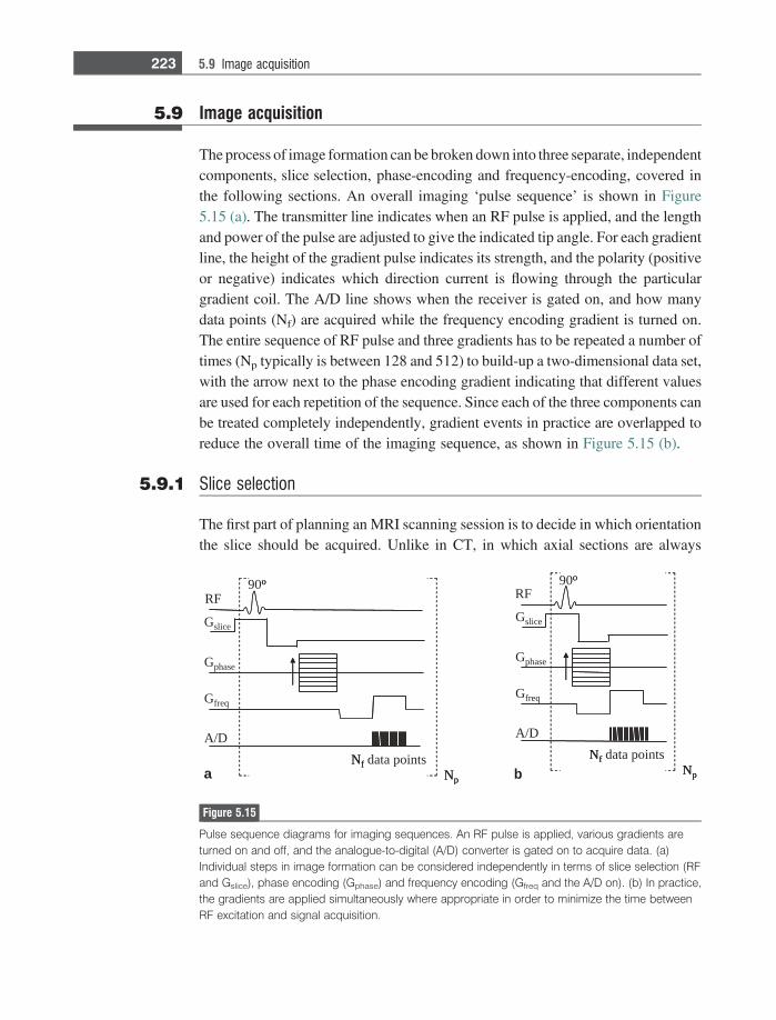
5.9 Image acquisition
The process of image formation can be broken down into three separate, independentcomponents, slice selection, phase-encoding and frequency-encoding, covered inthe following sections. An overall imaging ‘pulse sequence’ is shown in Figure5.15 (a). The transmitter line indicates when an RF pulse is applied, and the lengthand power of the pulse are adjusted to give the indicated tip angle. For each gradientline, the height of the gradient pulse indicates its strength, and the polarity (positiveor negative) indicates which direction current is flowing through the particulargradient coil. The A/D line shows when the receiver is gated on, and how manydata points (Nf) are acquired while the frequency encoding gradient is turned on.The entire sequence of RF pulse and three gradients has to be repeated a number oftimes (Np typically is between 128 and 512) to build-up a two-dimensional data set,with the arrow next to the phase encoding gradient indicating that different valuesare used for each repetition of the sequence. Since each of the three components canbe treated completely independently, gradient events in practice are overlapped toreduce the overall time of the imaging sequence, as shown in Figure 5.15 (b).
5.9.1 Slice selection
The first part of planning an MRI scanning session is to decide in which orientationthe slice should be acquired. Unlike in CT, in which axial sections are always
a b
90o
Nf data pointsNp
RF
Gphase
A/D
Gslice
Gfreq
90o
Nf data pointsNp
RF
Gphase
A/D
Gslice
Gfreq
o
NfNp
o
NfNp
Figure 5.15
Pulse sequence diagrams for imaging sequences. An RF pulse is applied, various gradients areturned on and off, and the analogue-to-digital (A/D) converter is gated on to acquire data. (a)Individual steps in image formation can be considered independently in terms of slice selection (RFand Gslice), phase encoding (Gphase) and frequency encoding (Gfreq and the A/D on). (b) In practice,the gradients are applied simultaneously where appropriate in order to minimize the time betweenRF excitation and signal acquisition.
223 5.9 Image acquisition
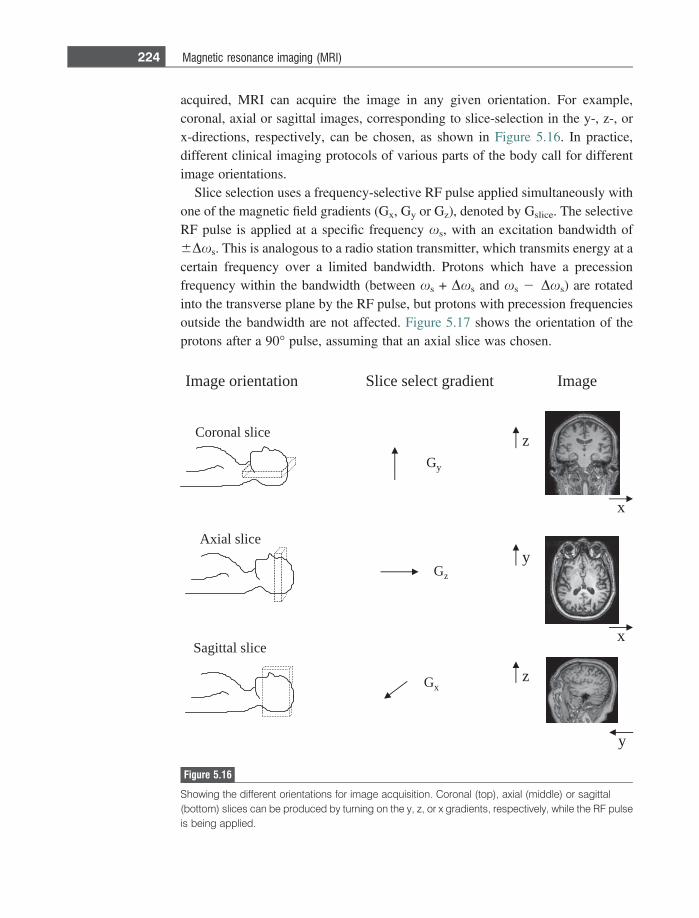
acquired, MRI can acquire the image in any given orientation. For example,coronal, axial or sagittal images, corresponding to slice-selection in the y-, z-, orx-directions, respectively, can be chosen, as shown in Figure 5.16. In practice,different clinical imaging protocols of various parts of the body call for differentimage orientations.
Slice selection uses a frequency-selective RF pulse applied simultaneously withone of the magnetic field gradients (Gx, Gy or Gz), denoted by Gslice. The selectiveRF pulse is applied at a specific frequency xs, with an excitation bandwidth of6Dxs. This is analogous to a radio station transmitter, which transmits energy at acertain frequency over a limited bandwidth. Protons which have a precessionfrequency within the bandwidth (between xs + Dxs and xs 2 Dxs) are rotatedinto the transverse plane by the RF pulse, but protons with precession frequenciesoutside the bandwidth are not affected. Figure 5.17 shows the orientation of theprotons after a 90� pulse, assuming that an axial slice was chosen.
ecils lanoroC
ecils laixA
ecilslattigaS
tneidarg tceles ecilS
Gz
Gy
Gx
egamInoitatneiro egamI
x
z
x
y
y
z
Figure 5.16
Showing the different orientations for image acquisition. Coronal (top), axial (middle) or sagittal(bottom) slices can be produced by turning on the y, z, or x gradients, respectively, while the RF pulseis being applied.
224 Magnetic resonance imaging (MRI)

The slice thickness (T) is given by:
T 52Dxs
cGslice: ð5:25Þ
The slice can therefore be made thinner either by increasing the strength of Gslice
(up to its maximum value) or decreasing the frequency bandwidth of the RF pulse.The ideal frequency excitation profile of the RF pulse is a rectangular shape, inwhich case an equal tip angle is applied to all the protons within the slice, and zerotip angle to protons outside the slice. Using the Fourier transform properties inSection 1.9.1, a sinc or similarly shaped RF pulse, typically with a length of a fewms, is used. The slice position can be moved to different parts of the patient bychanging the value of xs of the RF pulse.
Example 5.5 If the maximum gradient strength is 40 mT/m, calculate the bandwidth of the RFpulse necessary to give a 1 mm slice thickness. If the slice thickness is decreased to0.5 mm, is the required RF pulse shorter or longer than for a 1 mm slice thickness?
Solution Using Equation (5.23):
1 3 10�3 mð Þ 52Dxs
267:54 3 106 HzT�1ð Þ0:04 Tm�1ð Þ :
Solving gives a bandwidth 2Dxs of 10 070 rads21 or 1700 Hz.From the properties of the Fourier transform, a longer RF pulse results in anarrower frequency spectrum, and therefore the thinner slice requires an RF pulseof double the length for a given value of Gslice.
z
frequency
Slice thickness
Gslice
s− s
s + s
s
slice centre
− s
s + s
s
Figure 5.17
(left) The effects of a 90� RF pulse applied simultaneously with the z-gradient. Only protons withinthe axial slice are tipped by 90� into the transverse plane, and so give a measureable MR signal.Protons outside the chosen slice have their net magnetization remain in the z-direction. (right) Showingthe gradient strength (the slope of the graph) as a function of position in z.
225 5.9 Image acquisition
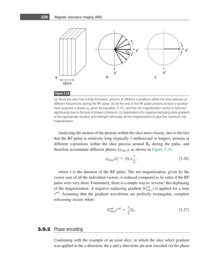
Analyzing the motion of the protons within the slice more closely, due to the factthat the RF pulse is relatively long (typically 1 millisecond or longer), protons atdifferent z-positions within the slice precess around B0 during the pulse, andtherefore accumulate different phases (uslice), as shown in Figure 5.18:
usliceðzÞ 5 cGzzs2; ð5:26Þ
where s is the duration of the RF pulse. The net magnetization, given by thevector sum of all the individual vectors, is reduced compared to its value if the RFpulse were very short. Fortunately, there is a simple way to ‘reverse’ this dephasingof the magnetization. A negative rephasing gradient (Gref
slice) is applied for a timesref. Assuming that the gradient waveforms are perfectly rectangular, completerefocusing occurs when:
Grefslices
ref 5s2
Gz: ð5:27Þ
5.9.2 Phase encoding
Continuing with the example of an axial slice, in which the slice select gradientwas applied in the z-direction, the x and y directions are now encoded via the phase
slice
x'
y'sl
x'
y'
x'
y'sl
x'
y'
a b c
Figure 5.18
(a) Since the slice has a finite thickness, protons at different z-positions within the slice precess atdifferent frequencies during the RF pulse. (b) At the end of the RF pulse protons at each z-positionhave acquired a phase usl given by Equation (5.26), and the net magnetization vector is reducedsignificantly due to the lack of phase coherence. (c) Application of a negative rephasing slice gradientof the appropriate duration and strength refocuses all the magnetization to give the maximum netmagnetization.
226 Magnetic resonance imaging (MRI)
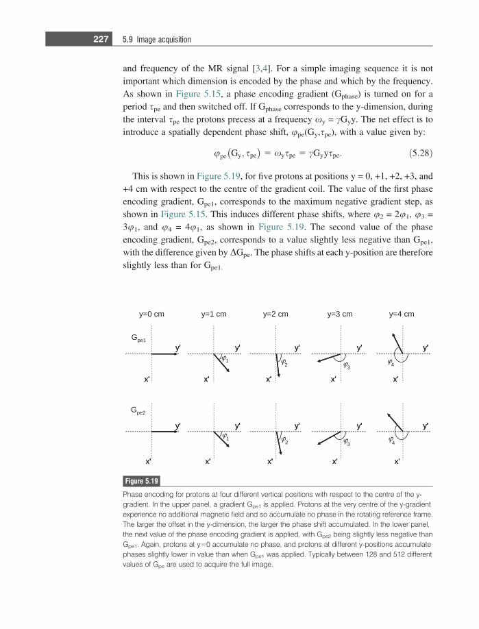
and frequency of the MR signal [3,4]. For a simple imaging sequence it is notimportant which dimension is encoded by the phase and which by the frequency.As shown in Figure 5.15, a phase encoding gradient (Gphase) is turned on for aperiod spe and then switched off. If Gphase corresponds to the y-dimension, duringthe interval spe the protons precess at a frequency xy = cGyy. The net effect is tointroduce a spatially dependent phase shift, upe(Gy,spe), with a value given by:
upe Gy; spe� �
5 xyspe 5 cGyyspe: ð5:28Þ
This is shown in Figure 5.19, for five protons at positions y = 0, +1, +2, +3, and+4 cm with respect to the centre of the gradient coil. The value of the first phaseencoding gradient, Gpe1, corresponds to the maximum negative gradient step, asshown in Figure 5.15. This induces different phase shifts, where u2 = 2u1, u3 =3u1, and u4 = 4u1, as shown in Figure 5.19. The second value of the phaseencoding gradient, Gpe2, corresponds to a value slightly less negative than Gpe1,with the difference given by DGpe. The phase shifts at each y-position are thereforeslightly less than for Gpe1.
y=1 cm y=2 cm y=3 cm y=4 cm
13 4
G pe1
12 3
G pe2
y=0 cm
x ' x ' x ' x ' x '
x' x' x' x' x'
y ' y ' y ' y ' y '
y ' y ' y ' y ' y '
2
4
x ' x ' x ' x ' x ' ' ' ' ' '
x' x' x' x' x'' ' ' '
y ' y ' y ' y ' y ' ' ' ' '
y ' y ' y ' y ' y ' ' ' ' ' '
Figure 5.19
Phase encoding for protons at four different vertical positions with respect to the centre of the y-gradient. In the upper panel, a gradient Gpe1 is applied. Protons at the very centre of the y-gradientexperience no additional magnetic field and so accumulate no phase in the rotating reference frame.The larger the offset in the y-dimension, the larger the phase shift accumulated. In the lower panel,the next value of the phase encoding gradient is applied, with Gpe2 being slightly less negative thanGpe1. Again, protons at y=0 accumulate no phase, and protons at different y-positions accumulatephases slightly lower in value than when Gpe1 was applied. Typically between 128 and 512 differentvalues of Gpe are used to acquire the full image.
227 5.9 Image acquisition
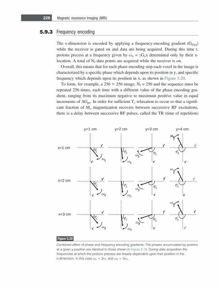
5.9.3 Frequency encoding
The x-dimension is encoded by applying a frequency-encoding gradient (Gfreq)while the receiver is gated on and data are being acquired. During this time t,protons precess at a frequency given by xx = cGxx determined only by their x-location. A total of Nf data points are acquired while the receiver is on.
Overall, this means that for each phase encoding step each voxel in the image ischaracterized by a specific phase which depends upon its position in y, and specificfrequency which depends upon its position in x, as shown in Figure 5.20.
To form, for example, a 256 3 256 image, Nf = 256 and the sequence must berepeated 256 times, each time with a different value of the phase encoding gra-dient, ranging from its maximum negative to maximum positive value in equalincrements of DGpe. In order for sufficient T1 relaxation to occur so that a signifi-cant fraction of Mz magnetization recovers between successive RF excitations,there is a delay between successive RF pulses, called the TR (time of repetition)
y=1 cm y=2 cm y=3 cm y=4 cm
1x=1 cm
x=2 cm
x=3 cm
1
ω 2
ω 3
1
ω 1
ω 1
ω 2
ω 3
ω 2
3
ω 2
ω 3
x '
y '
x '
y '
x '
y '
x '
y '
x '
y '
x '
y '
x '
y '
x '
y '
x '
y '
1
2
3
ω 1
1
ω 1
2
ω 3
3
ω 1 1
1
ω 1
3
x '
y
1
1
2
2
2
3
3
3
4
4
4
'
'
'
x '
y ' y '
x '
y '
'
y '
x '
y '
'
'
x '
'
'
'
'
y '
'
'
x '
'
x '
y '
'
'
x '
y '
'
'
Figure 5.20
Combined effect of phase and frequency encoding gradients. The phases accumulated by protonsat a given y-position are identical to those shown in Figure 5.19. During data acquisition thefrequencies at which the protons precess are linearly dependent upon their position in thex-dimension. In this case x2 = 2x1 and x3 = 3x1.
228 Magnetic resonance imaging (MRI)
time. Overall, the total data acquisition time is therefore given by the TR multipliedby the number of phase encoding steps applied, TR*Npe.
5.10 The k-space formalism and image reconstruction
To understand how the acquired data are transformed into an image, it is instructiveto express the (Nf 3 Npe) signals mathematically as
s Gy; spe;Gx; t� �
}
ðslice
ðslice
q x; yð Þe�jcGyyspe e�jcGxxtdxdy: ð5:29Þ
One can treat the slice, phase and frequency encoding terms independently. Thedouble integral over the slice represents the fact that signal comes only fromprotons within the slice, and that there is no signal from protons outside this slice.The factor q(x,y) is the number of protons at each position (x,y) within this slice,and is called the proton density. This can be related to the term Ntotal in Equation(5.10): the signal intensity is directly proportional to the number of protons in eachvoxel. The second term in the integral represents the phase term (uy = cGyyspe)from the phase encoding gradient. The third term in the equation represents thespatially dependent resonance frequency (xx = cGxx).
A very useful model is the ‘k-space’ formalism developed by Ljunggren [5].Two variables, kx and ky, are defined as:
kx 5c
2pGxt; ky 5
c2p
Gyspe: ð5:30Þ
The k values are spatial frequencies, as covered in Chapter 1. Equation (5.29)can now be expressed in terms of these two variables:
S kx; ky� �
}
ðslice
ðslice
q x; yð Þe�j2pkxxe�j2pkyydxdy: ð5:31Þ
The acquired data can therefore be represented as a two-dimensional data set inkx,ky-space. Consider the Nf data points collected when the maximum negativevalue of the phase-encoding gradient, Gy, is applied. From Equation (5.30) thevalue of ky for all Nf data points corresponds to its maximum negative value. Asshown in Figure 5.15, a negative gradient , is applied in the x-direction before dataacquisition. Denoting the strength of this gradient by Gdephase and the time forwhich it is applied by sdephase, then the values are chosen are chosen such that:
Gdephasesdephase 5Tacq
2Gfreq: ð5:32Þ
229 5.10 The k-space formalism and image reconstruction
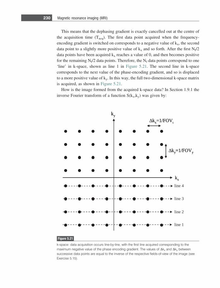
This means that the dephasing gradient is exactly cancelled out at the centre ofthe acquisition time (Tacq). The first data point acquired when the frequency-encoding gradient is switched on corresponds to a negative value of kx, the seconddata point to a slightly more positive value of kx and so forth. After the first Nf/2data points have been acquired kx reaches a value of 0, and then becomes positivefor the remaining Nf/2 data points. Therefore, the Nf data points correspond to one‘line’ in k-space, shown as line 1 in Figure 5.21. The second line in k-spacecorresponds to the next value of the phase-encoding gradient, and so is displacedto a more positive value of ky. In this way, the full two-dimensional k-space matrixis acquired, as shown in Figure 5.21.
How is the image formed from the acquired k-space data? In Section 1.9.1 theinverse Fourier transform of a function S(kx,ky) was given by:
kx
ky
Δkx=1/FOVx
Δky=1/FOVy
kx
ky
line 1
line 2
line 3
line 4
Δkx=1/FOV
Δky=1/FOVy
Figure 5.21
k-space: data acquisition occurs line-by-line, with the first line acquired corresponding to themaximum negative value of the phase encoding gradient. The values of Dkx and Dky betweensuccessive data points are equal to the inverse of the respective fields-of-view of the image (seeExercise 5.15).
230 Magnetic resonance imaging (MRI)
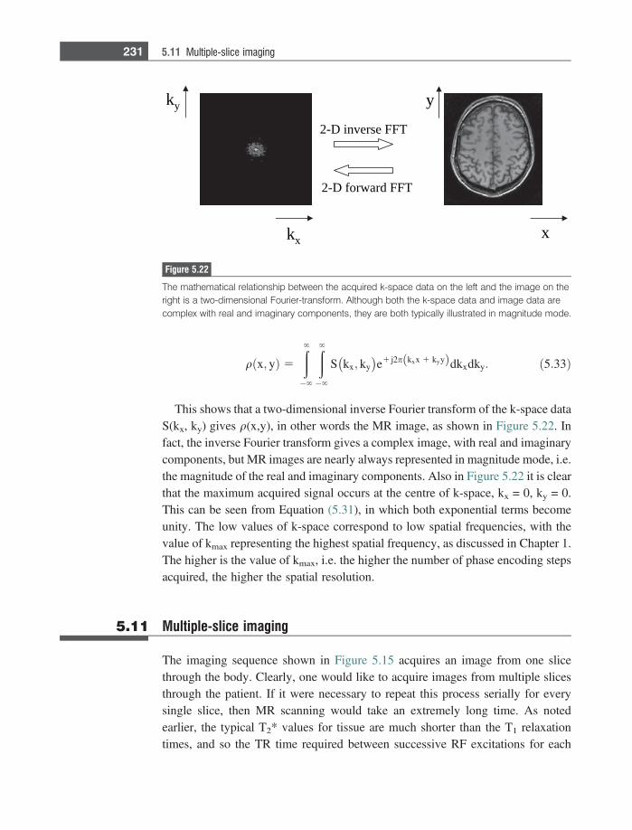
qðx; yÞ 5
�
�
S kx; ky� �
e1 j2p kxx 1 kyyð Þdkxdky: ð5:33Þ
This shows that a two-dimensional inverse Fourier transform of the k-space dataS(kx, ky) gives q(x,y), in other words the MR image, as shown in Figure 5.22. Infact, the inverse Fourier transform gives a complex image, with real and imaginarycomponents, but MR images are nearly always represented in magnitude mode, i.e.the magnitude of the real and imaginary components. Also in Figure 5.22 it is clearthat the maximum acquired signal occurs at the centre of k-space, kx = 0, ky = 0.This can be seen from Equation (5.31), in which both exponential terms becomeunity. The low values of k-space correspond to low spatial frequencies, with thevalue of kmax representing the highest spatial frequency, as discussed in Chapter 1.The higher is the value of kmax, i.e. the higher the number of phase encoding stepsacquired, the higher the spatial resolution.
5.11 Multiple-slice imaging
The imaging sequence shown in Figure 5.15 acquires an image from one slicethrough the body. Clearly, one would like to acquire images from multiple slicesthrough the patient. If it were necessary to repeat this process serially for everysingle slice, then MR scanning would take an extremely long time. As notedearlier, the typical T2* values for tissue are much shorter than the T1 relaxationtimes, and so the TR time required between successive RF excitations for each
kx
ky
x
y
TFF esrevni D-2
TFF drawrof D-2
Figure 5.22
The mathematical relationship between the acquired k-space data on the left and the image on theright is a two-dimensional Fourier-transform. Although both the k-space data and image data arecomplex with real and imaginary components, they are both typically illustrated in magnitude mode.
231 5.11 Multiple-slice imaging
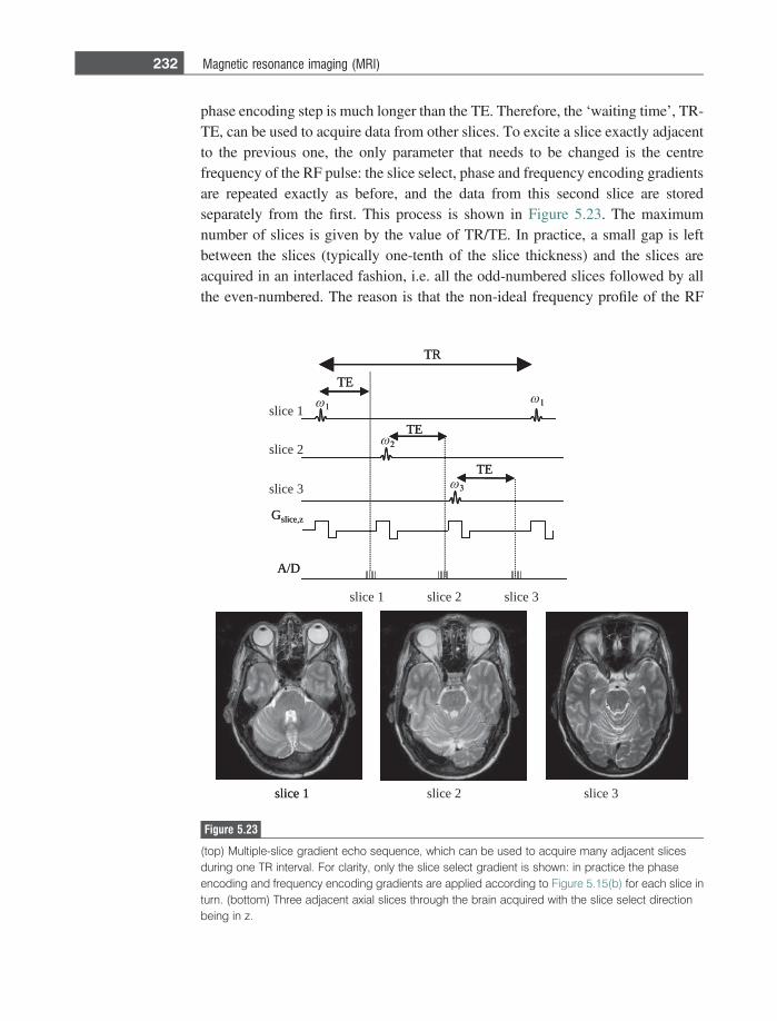
phase encoding step is much longer than the TE. Therefore, the ‘waiting time’, TR-TE, can be used to acquire data from other slices. To excite a slice exactly adjacentto the previous one, the only parameter that needs to be changed is the centrefrequency of the RF pulse: the slice select, phase and frequency encoding gradientsare repeated exactly as before, and the data from this second slice are storedseparately from the first. This process is shown in Figure 5.23. The maximumnumber of slices is given by the value of TR/TE. In practice, a small gap is leftbetween the slices (typically one-tenth of the slice thickness) and the slices areacquired in an interlaced fashion, i.e. all the odd-numbered slices followed by allthe even-numbered. The reason is that the non-ideal frequency profile of the RF
slice 1 slice 2 slice 3
slice 2
slice 3
TR
TE
A/D
TE
TE
2
3
slice 1 1 1
Gslice,z
slice 1 slice 2 slice 3
slice 1
TR
TE
A/D
TE
TE
2
3
1 1
Gslice,z
Figure 5.23
(top) Multiple-slice gradient echo sequence, which can be used to acquire many adjacent slicesduring one TR interval. For clarity, only the slice select gradient is shown: in practice the phaseencoding and frequency encoding gradients are applied according to Figure 5.15(b) for each slice inturn. (bottom) Three adjacent axial slices through the brain acquired with the slice select directionbeing in z.
232 Magnetic resonance imaging (MRI)
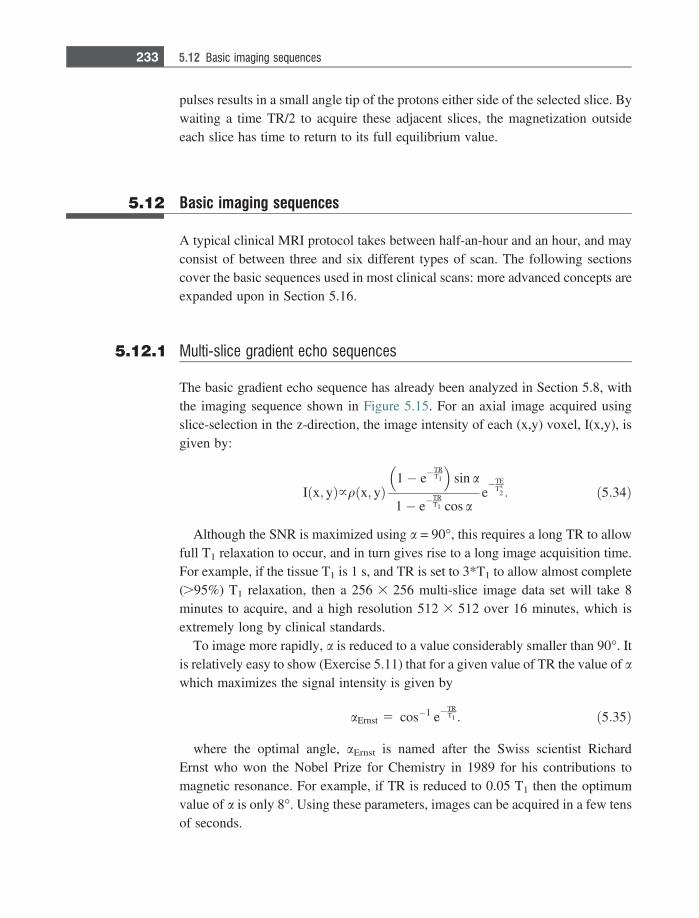
pulses results in a small angle tip of the protons either side of the selected slice. Bywaiting a time TR/2 to acquire these adjacent slices, the magnetization outsideeach slice has time to return to its full equilibrium value.
5.12 Basic imaging sequences
A typical clinical MRI protocol takes between half-an-hour and an hour, and mayconsist of between three and six different types of scan. The following sectionscover the basic sequences used in most clinical scans: more advanced concepts areexpanded upon in Section 5.16.
5.12.1 Multi-slice gradient echo sequences
The basic gradient echo sequence has already been analyzed in Section 5.8, withthe imaging sequence shown in Figure 5.15. For an axial image acquired usingslice-selection in the z-direction, the image intensity of each (x,y) voxel, I(x,y), isgiven by:
I x; yð Þ}q x; yð Þ1� e�
TRT1
� �sin a
1� e�TRT1 cos a
e�TE
T�2 : ð5:34Þ
Although the SNR is maximized using a = 90�, this requires a long TR to allowfull T1 relaxation to occur, and in turn gives rise to a long image acquisition time.For example, if the tissue T1 is 1 s, and TR is set to 3*T1 to allow almost complete(.95%) T1 relaxation, then a 256 3 256 multi-slice image data set will take 8minutes to acquire, and a high resolution 512 3 512 over 16 minutes, which isextremely long by clinical standards.
To image more rapidly, a is reduced to a value considerably smaller than 90�. Itis relatively easy to show (Exercise 5.11) that for a given value of TR the value of awhich maximizes the signal intensity is given by
aErnst 5 cos�1 e�TRT1 : ð5:35Þ
where the optimal angle, aErnst is named after the Swiss scientist RichardErnst who won the Nobel Prize for Chemistry in 1989 for his contributions tomagnetic resonance. For example, if TR is reduced to 0.05 T1 then the optimumvalue of a is only 8�. Using these parameters, images can be acquired in a few tensof seconds.
233 5.12 Basic imaging sequences
Example 5.6 For a TR time equal to the T1 value of the tissue, what angle should used for the RFpulse to maximize the SNR? How much greater is the SNR than would have beenachieved had the RF pulse mistakenly been set to 90�?
Solution The optimal angle is given by:
aErnst 5 cos�1 e�1 5 cos�1 0:3679ð Þ 5 68o:
Plugging this value into Equation (5.34) gives an I(x,y) value of 0.68q(x,y)e2TE/T2.If an angle of 90� had been used, then this value would have been 0.63 q(x,y)e2TE/T2.
From Equation (5.34) one can see that there are three separate components thataffect the signal intensity: the proton density, a combination of the TR,T1 and avalues, and the TE and T2* values. The data acquisition parameters in a gradient-echo sequence can be set to emphasize, or ‘weight’, the image intensity by one orall of the tissue parameters q(x,y), T1 or T2*, depending upon the choice of dataacquisition parameters. For example, suppose that we are trying to differentiatebetween two tissues A and B. The proton density for A is 1.0, and for B is 1.2. TheT1 value for A is 1 s and that of B is 1.3 s. Finally, the T2* of A is 35 ms, and of B is30 ms. If the value of TE is set to 1 ms, then the relative signals due to T2* decayalone are 0.972 and 0.967 for A and B respectively, a very small difference.Therefore, the image intensity is not ‘weighted’ by the different values of T2*for tissues A and B. In contrast, if TE is set to 30 ms, then the signals are 0.368 and0.424 which is a much larger difference: the image can now be said to be T2*-weighted. Similarly, for a given value of TR, the higher the value of a the higherthe T1-weighting of the image, i.e. the greater the extent to which the relativeintensities of tissues A and B depend upon the respective T1 values. Alternatively,for a fixed a the shorter the TR the higher is the T1-weighting. Finally, the protondensity of course cannot be changed, since it is a fixed physical value. Ifthe sequence parameters are chosen so that there is no T1-weighting and noT2*-weighting, then the image is said to be proton-density weighted. Table 5.2shows the possible combinations of imaging parameters and the correspondingweighting.
5.12.2 Spin echo sequences
Gradient-echo sequences allow very rapid image acquisition. The major disadvant-age is that they do not allow images to be weighted by the different T2 values, butrather only by the T2*value. Since, as discussed previously, T2* values are typi-cally much shorter than T2 this leads not only to lower signal intensities than if one
234 Magnetic resonance imaging (MRI)
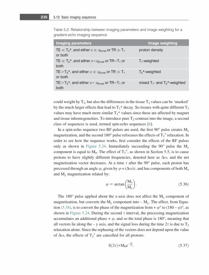
could weight by T2, but also the differences in the tissue T2 values can be ‘masked’by the much larger effects that lead to T2* decay. So tissues with quite different T2
values may have much more similar T2* values since these are affected by magnetand tissue inhomogeneities. To introduce pure T2-contrast into the image, a secondclass of sequences is used, termed spin-echo sequences [6].
In a spin-echo sequence two RF pulses are used, the first 90� pulse creates My
magnetization, and the second 180� pulse refocuses the effects of T2+ relaxation. In
order to see how the sequence works, first consider the effects of the RF pulsesonly as shown in Figure 5.24. Immediately succeeding the 90� pulse the My
component is equal to M0. The effect of T2+, as shown in Section 5.5, is to cause
protons to have slightly different frequencies, denoted here as Dx, and the netmagnetization vector decreases. At a time s after the 90� pulse, each proton hasprecessed through an angle u, given by u = (Dx)s, and has components of both Mx
and My magnetization related by:
u 5 arctanMx
My
� �: ð5:36Þ
The 180� pulse applied about the x-axis does not affect the Mx component ofmagnetization, but converts the My component into – My. The effect, from Equa-tion (5.34), is to convert the phase of the magnetization from + u� to (180 – u)�, asshown in Figure 5.24. During the second s interval, the precessing magnetizationaccumulates an additional phase + u, and so the total phase is 180�, meaning thatall vectors lie along the – y axis, and the signal loss during the time 2s is due to T2
relaxation alone. Since the rephasing of the vectors does not depend upon the valueof Dx, the effects of T2
+ are cancelled for all protons:
Sð2sÞ}M0e�2sT2 : ð5:37Þ
Table 5.2: Relationship between imaging parameters and image weighting for agradient-echo imaging sequence
Imaging parameters Image weighting
TE� T2*, and either a� aErnst or TR� T1
or bothproton density
TE� T2*, and either a~aErnst or TR~T1 orboth
T1-weighted
TE.T2*, and either a� aErnst or TR� T1
or bothT2*-weighted
TE.T2*, and either a~ aErnst or TR~T1 orboth
mixed T1- and T2*-weighted
235 5.12 Basic imaging sequences
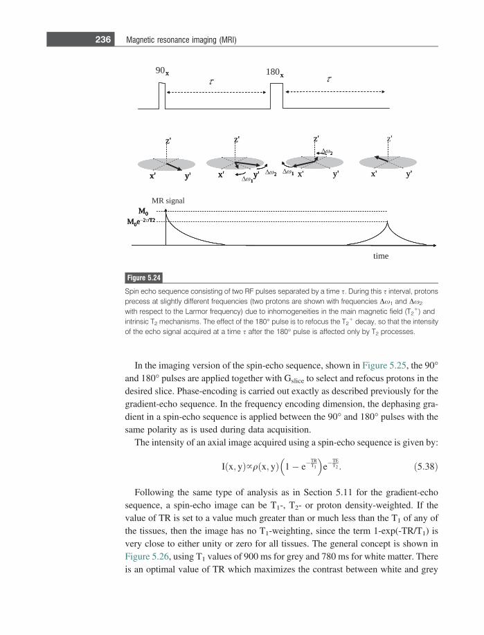
In the imaging version of the spin-echo sequence, shown in Figure 5.25, the 90�and 180� pulses are applied together with Gslice to select and refocus protons in thedesired slice. Phase-encoding is carried out exactly as described previously for thegradient-echo sequence. In the frequency encoding dimension, the dephasing gra-dient in a spin-echo sequence is applied between the 90� and 180� pulses with thesame polarity as is used during data acquisition.
The intensity of an axial image acquired using a spin-echo sequence is given by:
I x; yð Þ}q x; yð Þ 1� e�TRT1
� �e�
TET2 : ð5:38Þ
Following the same type of analysis as in Section 5.11 for the gradient-echosequence, a spin-echo image can be T1-, T2- or proton density-weighted. If thevalue of TR is set to a value much greater than or much less than the T1 of any ofthe tissues, then the image has no T1-weighting, since the term 1-exp(-TR/T1) isvery close to either unity or zero for all tissues. The general concept is shown inFigure 5.26, using T1 values of 900 ms for grey and 780 ms for white matter. Thereis an optimal value of TR which maximizes the contrast between white and grey
x' y'
z'
x' y'
z'
1
2 x' y'
z'
1
2
x' y'
z'
90x 180x
time
MR signal
M0e2 /T2
M0
x' y'
z'
x' y'
z'
1
2 x' y'
z'
1
2
x' y'x' y'x' y' x' y'1
2x' y'1
2 1
2
1
2
x xx x
M0e2 /T2
M0
M0e/T2
M0
0−2 /T2
M0
Figure 5.24
Spin echo sequence consisting of two RF pulses separated by a time s. During this s interval, protonsprecess at slightly different frequencies (two protons are shown with frequencies Dx1 and Dx2
with respect to the Larmor frequency) due to inhomogeneities in the main magnetic field (T2+) and
intrinsic T2 mechanisms. The effect of the 180� pulse is to refocus the T2+ decay, so that the intensity
of the echo signal acquired at a time s after the 180� pulse is affected only by T2 processes.
236 Magnetic resonance imaging (MRI)
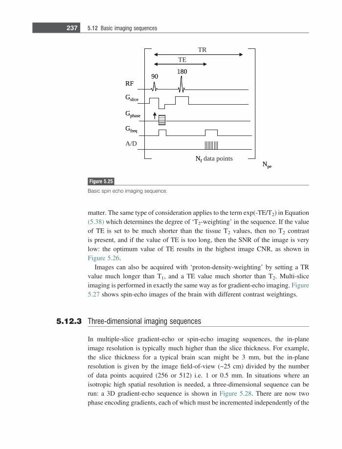
matter. The same type of consideration applies to the term exp(-TE/T2) in Equation(5.38) which determines the degree of ‘T2-weighting’ in the sequence. If the valueof TE is set to be much shorter than the tissue T2 values, then no T2 contrastis present, and if the value of TE is too long, then the SNR of the image is verylow: the optimum value of TE results in the highest image CNR, as shown inFigure 5.26.
Images can also be acquired with ‘proton-density-weighting’ by setting a TRvalue much longer than T1, and a TE value much shorter than T2. Multi-sliceimaging is performed in exactly the same way as for gradient-echo imaging. Figure5.27 shows spin-echo images of the brain with different contrast weightings.
5.12.3 Three-dimensional imaging sequences
In multiple-slice gradient-echo or spin-echo imaging sequences, the in-planeimage resolution is typically much higher than the slice thickness. For example,the slice thickness for a typical brain scan might be 3 mm, but the in-planeresolution is given by the image field-of-view (~25 cm) divided by the numberof data points acquired (256 or 512) i.e. 1 or 0.5 mm. In situations where anisotropic high spatial resolution is needed, a three-dimensional sequence can berun: a 3D gradient-echo sequence is shown in Figure 5.28. There are now twophase encoding gradients, each of which must be incremented independently of the
TETR
90180
RF
Gfreq
Gphase
Gslice
A/D
NpeNf data points
90180
RF
Gfreq
Gphase
Gslice
NpeNf
Figure 5.25
Basic spin echo imaging sequence.
237 5.12 Basic imaging sequences
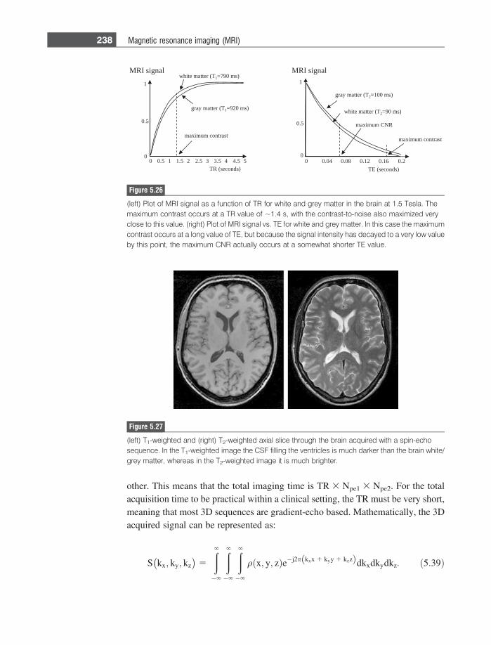
other. This means that the total imaging time is TR 3 Npe1 3 Npe2. For the totalacquisition time to be practical within a clinical setting, the TR must be very short,meaning that most 3D sequences are gradient-echo based. Mathematically, the 3Dacquired signal can be represented as:
S kx; ky; kz� �
5
�
�
�
qðx; y; zÞe�j2p kxx 1 kyy 1 kzzð Þdkxdkydkz: ð5:39Þ
0 0.5 1 1.5 2 2.5 3 3.5 4 4.5 50
0.5
1
TR (seconds)
MRI signal
gray matter (T1=920 ms)
white matter (T1=790 ms)
maximum contrast
0 0.04 0.08 0.12 0.16 0.2
0.5
1
TE (seconds)
MRI signal
0
maximum CNR
maximum contrast
gray matter (T2=100 ms)
white matter (T2=90 ms)
Figure 5.26
(left) Plot of MRI signal as a function of TR for white and grey matter in the brain at 1.5 Tesla. Themaximum contrast occurs at a TR value of ~1.4 s, with the contrast-to-noise also maximized veryclose to this value. (right) Plot of MRI signal vs. TE for white and grey matter. In this case the maximumcontrast occurs at a long value of TE, but because the signal intensity has decayed to a very low valueby this point, the maximum CNR actually occurs at a somewhat shorter TE value.
Figure 5.27
(left) T1-weighted and (right) T2-weighted axial slice through the brain acquired with a spin-echosequence. In the T1-weighted image the CSF filling the ventricles is much darker than the brain white/grey matter, whereas in the T2-weighted image it is much brighter.
238 Magnetic resonance imaging (MRI)
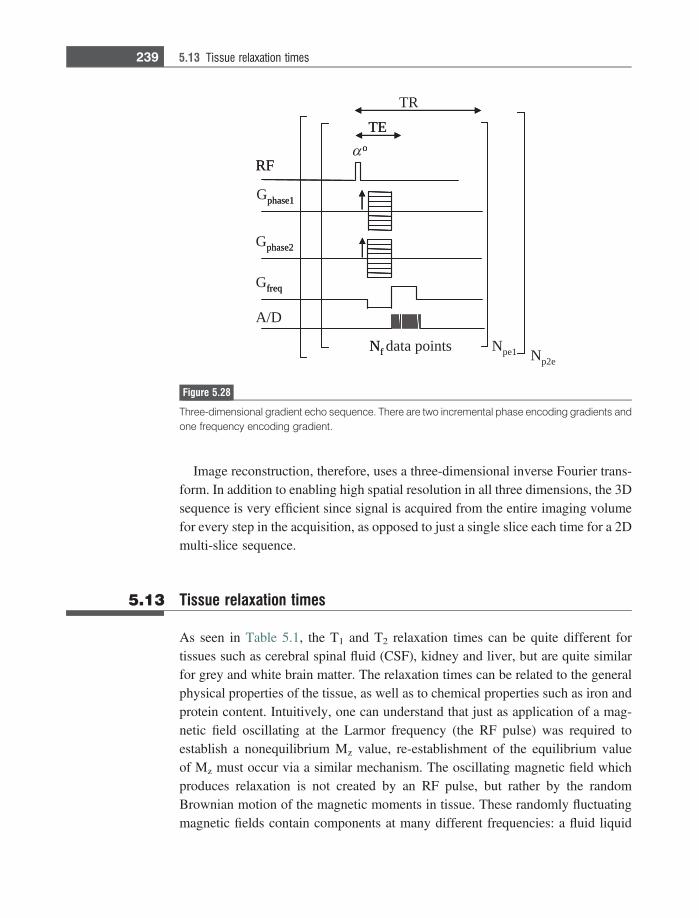
Image reconstruction, therefore, uses a three-dimensional inverse Fourier trans-form. In addition to enabling high spatial resolution in all three dimensions, the 3Dsequence is very efficient since signal is acquired from the entire imaging volumefor every step in the acquisition, as opposed to just a single slice each time for a 2Dmulti-slice sequence.
5.13 Tissue relaxation times
As seen in Table 5.1, the T1 and T2 relaxation times can be quite different fortissues such as cerebral spinal fluid (CSF), kidney and liver, but are quite similarfor grey and white brain matter. The relaxation times can be related to the generalphysical properties of the tissue, as well as to chemical properties such as iron andprotein content. Intuitively, one can understand that just as application of a mag-netic field oscillating at the Larmor frequency (the RF pulse) was required toestablish a nonequilibrium Mz value, re-establishment of the equilibrium valueof Mz must occur via a similar mechanism. The oscillating magnetic field whichproduces relaxation is not created by an RF pulse, but rather by the randomBrownian motion of the magnetic moments in tissue. These randomly fluctuatingmagnetic fields contain components at many different frequencies: a fluid liquid
α o
TRTE
RF
A/D
Gphase2
Gfreq
Gphase1
Npe1 Np2eNf data points
o
TE
RF
phase2
freq
phase1
Nf
Figure 5.28
Three-dimensional gradient echo sequence. There are two incremental phase encoding gradients andone frequency encoding gradient.
239 5.13 Tissue relaxation times
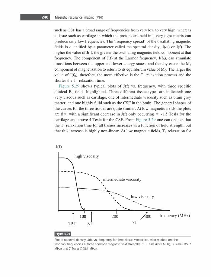
such as CSF has a broad range of frequencies from very low to very high, whereasa tissue such as cartilage in which the protons are held in a very tight matrix canproduce only low frequencies. The ‘frequency spread’ of the oscillating magneticfields is quantified by a parameter called the spectral density, J(x) or J(f). Thehigher the value of J(f), the greater the oscillating magnetic field component at thatfrequency. The component of J(f) at the Larmor frequency, J(f0), can stimulatetransitions between the upper and lower energy states, and thereby cause the Mz
component of magnetization to return to its equilibrium value of M0. The larger thevalue of J(f0), therefore, the more effective is the T1 relaxation process and theshorter the T1 relaxation time.
Figure 5.29 shows typical plots of J(f) vs. frequency, with three specificclinical B0 fields highlighted. Three different tissue types are indicated: onevery viscous such as cartilage, one of intermediate viscosity such as brain greymatter, and one highly fluid such as the CSF in the brain. The general shapes ofthe curves for the three tissues are quite similar. At low magnetic fields the plotsare flat, with a significant decrease in J(f) only occurring at ~1.5 Tesla for thecartilage and above 4 Tesla for the CSF. From Figure 5.29 one can deduce thatthe T1 relaxation time for all tissues increases as a function of field strength, butthat this increase is highly non-linear. At low magnetic fields, T1 relaxation for
high viscosity
intermediate viscosity
low viscosity
J(f)
100 200 300
1.5T 3T 7Tfrequency (MHz)
)
100
1.5T 3T
Figure 5.29
Plot of spectral density, J(f), vs. frequency for three tissue viscosities. Also marked are theresonant frequencies at three common magnetic field strengths, 1.5 Tesla (63.9 MHz), 3 Tesla (127.7MHz) and 7 Tesla (298.1 MHz).
240 Magnetic resonance imaging (MRI)
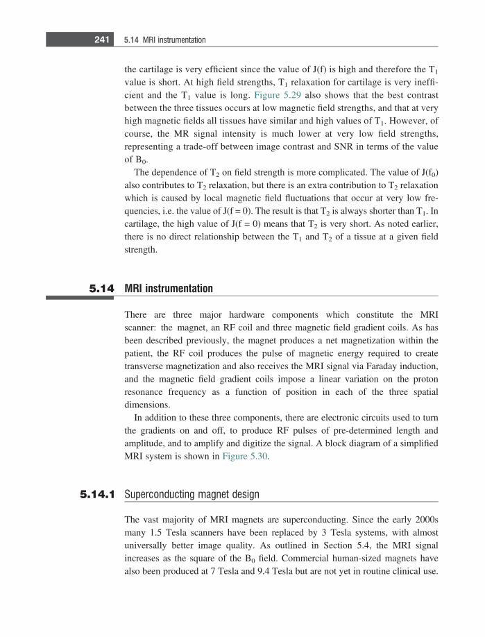
the cartilage is very efficient since the value of J(f) is high and therefore the T1
value is short. At high field strengths, T1 relaxation for cartilage is very ineffi-cient and the T1 value is long. Figure 5.29 also shows that the best contrastbetween the three tissues occurs at low magnetic field strengths, and that at veryhigh magnetic fields all tissues have similar and high values of T1. However, ofcourse, the MR signal intensity is much lower at very low field strengths,representing a trade-off between image contrast and SNR in terms of the valueof B0.
The dependence of T2 on field strength is more complicated. The value of J(f0)also contributes to T2 relaxation, but there is an extra contribution to T2 relaxationwhich is caused by local magnetic field fluctuations that occur at very low fre-quencies, i.e. the value of J(f = 0). The result is that T2 is always shorter than T1. Incartilage, the high value of J(f = 0) means that T2 is very short. As noted earlier,there is no direct relationship between the T1 and T2 of a tissue at a given fieldstrength.
5.14 MRI instrumentation
There are three major hardware components which constitute the MRIscanner: the magnet, an RF coil and three magnetic field gradient coils. As hasbeen described previously, the magnet produces a net magnetization within thepatient, the RF coil produces the pulse of magnetic energy required to createtransverse magnetization and also receives the MRI signal via Faraday induction,and the magnetic field gradient coils impose a linear variation on the protonresonance frequency as a function of position in each of the three spatialdimensions.
In addition to these three components, there are electronic circuits used to turnthe gradients on and off, to produce RF pulses of pre-determined length andamplitude, and to amplify and digitize the signal. A block diagram of a simplifiedMRI system is shown in Figure 5.30.
5.14.1 Superconducting magnet design
The vast majority of MRI magnets are superconducting. Since the early 2000smany 1.5 Tesla scanners have been replaced by 3 Tesla systems, with almostuniversally better image quality. As outlined in Section 5.4, the MRI signalincreases as the square of the B0 field. Commercial human-sized magnets havealso been produced at 7 Tesla and 9.4 Tesla but are not yet in routine clinical use.
241 5.14 MRI instrumentation
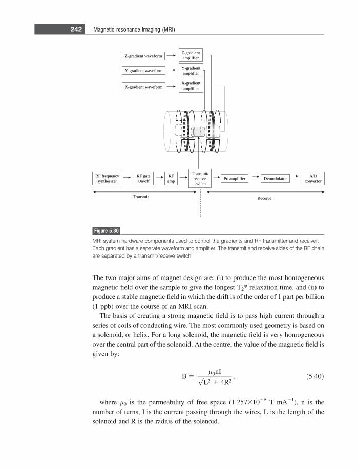
The two major aims of magnet design are: (i) to produce the most homogeneousmagnetic field over the sample to give the longest T2* relaxation time, and (ii) toproduce a stable magnetic field in which the drift is of the order of 1 part per billion(1 ppb) over the course of an MRI scan.
The basis of creating a strong magnetic field is to pass high current through aseries of coils of conducting wire. The most commonly used geometry is based ona solenoid, or helix. For a long solenoid, the magnetic field is very homogeneousover the central part of the solenoid. At the centre, the value of the magnetic field isgiven by:
B 5l0nIffiffiffiffiffiffiffiffiffiffiffiffiffiffiffiffiffiffiffi
L2 1 4R2p , ð5:40Þ
where l0 is the permeability of free space (1.25731026 T mA21), n is thenumber of turns, I is the current passing through the wires, L is the length of thesolenoid and R is the radius of the solenoid.
mrofevaw tneidarg-Xtneidarg-X
reifilpma
ycneuqerf FRrezisehtnys
/timsnarTeviecerhctiws
FRpma reifilpmaerP rotaludomeD D/A
rotrevnoc
timsnarT evieceR
tneidarg-Yreifilpma
tneidarg-Zreifilpma
mrofevaw tneidarg-Y
mrofevaw tneidarg-Z
etag FRffo/nO
Figure 5.30
MRI system hardware components used to control the gradients and RF transmitter and receiver.Each gradient has a separate waveform and amplifier. The transmit and receive sides of the RF chainare separated by a transmit/receive switch.
242 Magnetic resonance imaging (MRI)
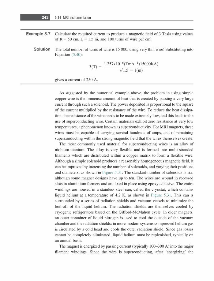
Example 5.7 Calculate the required current to produce a magnetic field of 3 Tesla using valuesof R = 50 cm, L = 1.5 m, and 100 turns of wire per cm.
Solution The total number of turns of wire is 15 000, using very thin wire! Substituting intoEquation (5.40):
3 Tð Þ 51:257x10�6 TmA�1ð Þ15000I Að Þffiffiffiffiffiffiffiffiffiffiffiffiffiffiffiffi
1:5 1 1p
mð Þ
gives a current of 250 A.
As suggested by the numerical example above, the problem in using simplecopper wire is the immense amount of heat that is created by passing a very largecurrent through such a solenoid. The power deposited is proportional to the squareof the current multiplied by the resistance of the wire. To reduce the heat dissipa-tion, the resistance of the wire needs to be made extremely low, and this leads to theuse of superconducting wire. Certain materials exhibit zero resistance at very lowtemperatures, a phenomenon known as superconductivity. For MRI magnets, thesewires must be capable of carrying several hundreds of amps, and of remainingsuperconducting within the strong magnetic field that the wires themselves create.
The most commonly used material for superconducting wires is an alloy ofniobium-titanium. The alloy is very flexible and is formed into multi-strandedfilaments which are distributed within a copper matrix to form a flexible wire.Although a simple solenoid produces a reasonably homogeneous magnetic field, itcan be improved by increasing the number of solenoids, and varying their positionsand diameters, as shown in Figure 5.31. The standard number of solenoids is six,although some magnet designs have up to ten. The wires are wound in recessedslots in aluminium formers and are fixed in place using epoxy adhesive. The entirewindings are housed in a stainless steel can, called the cryostat, which containsliquid helium at a temperature of 4.2 K, as shown in Figure 5.31. This can issurrounded by a series of radiation shields and vacuum vessels to minimize theboil-off of the liquid helium. The radiation shields are themselves cooled bycryogenic refrigerators based on the Gifford-McMahon cycle. In older magnets,an outer container of liquid nitrogen is used to cool the outside of the vacuumchamber and the radiation shields: in more modern systems compressed helium gasis circulated by a cold head and cools the outer radiation shield. Since gas lossescannot be completely eliminated, liquid helium must be replenished, typically onan annual basis.
The magnet is energized by passing current (typically 100–300 A) into the majorfilament windings. Since the wire is superconducting, after ‘energizing’ the
243 5.14 MRI instrumentation
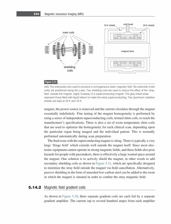
magnet, the power source is removed and the current circulates through the magnetessentially indefinitely. Fine tuning of the magnet homogeneity is performed byusing a series of independent superconducting coils, termed shim coils, to reach themanufacturer’s specifications. There is also a set of room temperature shim coilsthat are used to optimize the homogeneity for each clinical scan, depending uponthe particular organ being imaged and the individual patient. This is normallyperformed automatically during scan preparation.
The final issue with the superconducting magnet is siting. There is typically a verylarge ‘fringe field’ which extends well outside the magnet itself. Since most elec-tronic equipment cannot operate in strong magnetic fields, and these fields also posehazards for people with pacemakers, there is effectively a large wasted space aroundthe magnet. One solution is to actively shield the magnet, in other words to addsecondary shielding coils as shown in Figure 5.31, which are specifically designedto minimize the stray field outside the magnet via field cancellation. Alternatively,passive shielding in the form of annealed low-carbon steel can be added to the roomin which the magnet is situated in order to confine the stray magnetic field.
5.14.2 Magnetic field gradient coils
As shown in Figure 5.30, three separate gradient coils are each fed by a separategradient amplifier. The current (up to several hundred amps) from each amplifier
main coils
70 K shield cold head 20 K shield
magnet bore
shielding coils
Figure 5.31
(left) The solenoidal coils used to produce a homogeneous static magnetic field. Six solenoids (maincoils) are positioned along the z-axis. Two shielding coils are used to reduce the effect of the ‘strayfield’ outside the magnet. (right) Cutaway of a superconducting magnet. The grey tinted areasrepresent those filled with liquid helium to make the wires superconducting. Two aluminium radiationshields are kept at 20 K and 70 K.
244 Magnetic resonance imaging (MRI)
can be switched on and off in less than 1 ms. The maximum gradient strengthdepends upon the maximum current that can be passed through the gradient coilswithout causing excessive heating. The gradient coils are constructed of copper andare usually water-cooled. They are wound on cylindrical formers, which are boltedto the inner bore of the magnet. Currents passing through the coils cause alternatingLorenz forces within the magnetic field, and these forces must be balanced to avoidputting a large strain on the gradients. In fact, the loud sound of an MRI scan resultsfrom the whole cylinder vibrating, and these vibrations being translated to verycomplicated motions of the other components within the MRI system throughmechanical contact [7]. Acoustic damping is used, but the sound levels are stillwell above 100 dB and so the use of earplugs and headphones is mandatory.
The aims in gradient coil design are: (i) to produce the maximum gradient perunit current, (ii) to minimize the ‘rise’ time of the gradient, i.e. how fast it can reachits prescribed value, and (iii) to achieve the maximum volume of gradient linearity,usually defined as being 95% of the value in the exact centre of the gradient coil.Very simple designs, such as are shown in Figure 5.32, can be derived fromanalytical expressions for the magnetic fields created by loops of wire. The sim-plest configuration for the coil producing a gradient in the z-direction is a ‘Maxwellpair’, shown on the left of Figure 5.32, which consists of two loops each consistingof multiple turns of wire. The two loops are wound in opposite directions around acylindrical former, and the loops are spaced by a separation of O3 times the radius
z2 0
d
a
I Iz z
a b
Figure 5.32
(a) Basic geometry of a Maxwell-pair gradient coil which produces a magnetic field gradient in the z-direction. The two halves consist of equal numbers of turns of wire, with equal currents in each half butflowing in opposite directions. The magnetic fields from the two halves cancel in the centre of thegradient set. In the configuration shown, the left-hand half produces a magnetic field opposite to B0
(using Fleming’s left-hand rule) and therefore the resonant frequency increases in the positivez-direction. (b) Basic saddle-geometry for producing a transverse gradient, in this case in they-direction. The direction of current in the four identical components of the gradient coil is indicated bythe arrows. The design for producing an x-gradient is the same, but rotated by 90�.
245 5.14 MRI instrumentation
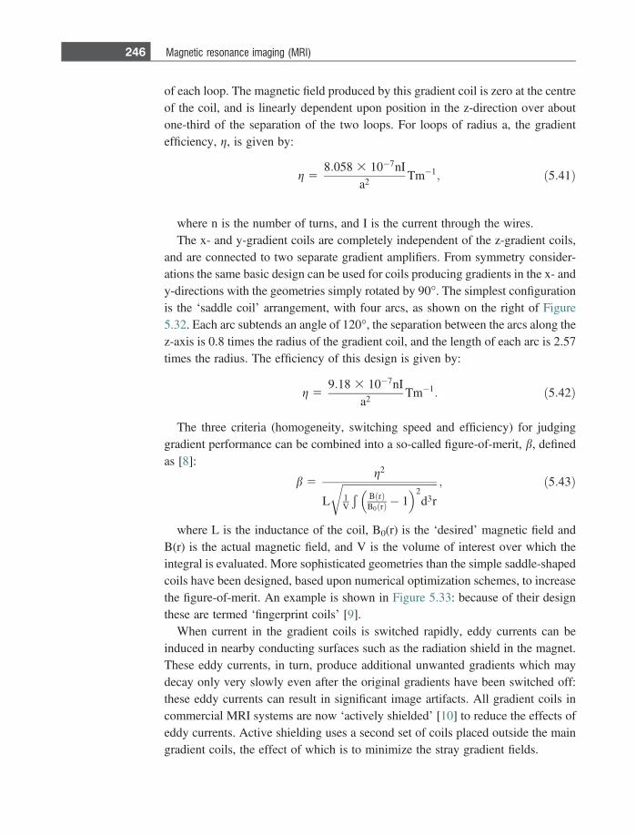
of each loop. The magnetic field produced by this gradient coil is zero at the centreof the coil, and is linearly dependent upon position in the z-direction over aboutone-third of the separation of the two loops. For loops of radius a, the gradientefficiency, g, is given by:
g 58:058 3 10�7nI
a2Tm�1; ð5:41Þ
where n is the number of turns, and I is the current through the wires.The x- and y-gradient coils are completely independent of the z-gradient coils,
and are connected to two separate gradient amplifiers. From symmetry consider-ations the same basic design can be used for coils producing gradients in the x- andy-directions with the geometries simply rotated by 90�. The simplest configurationis the ‘saddle coil’ arrangement, with four arcs, as shown on the right of Figure5.32. Each arc subtends an angle of 120�, the separation between the arcs along thez-axis is 0.8 times the radius of the gradient coil, and the length of each arc is 2.57times the radius. The efficiency of this design is given by:
g 59:18 3 10�7nI
a2Tm�1: ð5:42Þ
The three criteria (homogeneity, switching speed and efficiency) for judginggradient performance can be combined into a so-called figure-of-merit, b, definedas [8]:
b 5g2
L
ffiffiffiffiffiffiffiffiffiffiffiffiffiffiffiffiffiffiffiffiffiffiffiffiffiffiffiffiffiffiffiffiffiffiffiffi1V
Ð B rð ÞB0 rð Þ � 1� �2
d3r
r ; ð5:43Þ
where L is the inductance of the coil, B0(r) is the ‘desired’ magnetic field andB(r) is the actual magnetic field, and V is the volume of interest over which theintegral is evaluated. More sophisticated geometries than the simple saddle-shapedcoils have been designed, based upon numerical optimization schemes, to increasethe figure-of-merit. An example is shown in Figure 5.33: because of their designthese are termed ‘fingerprint coils’ [9].
When current in the gradient coils is switched rapidly, eddy currents can beinduced in nearby conducting surfaces such as the radiation shield in the magnet.These eddy currents, in turn, produce additional unwanted gradients which maydecay only very slowly even after the original gradients have been switched off:these eddy currents can result in significant image artifacts. All gradient coils incommercial MRI systems are now ‘actively shielded’ [10] to reduce the effects ofeddy currents. Active shielding uses a second set of coils placed outside the maingradient coils, the effect of which is to minimize the stray gradient fields.
246 Magnetic resonance imaging (MRI)
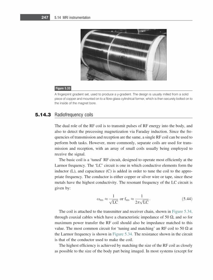
5.14.3 Radiofrequency coils
The dual role of the RF coil is to transmit pulses of RF energy into the body, andalso to detect the precessing magnetization via Faraday induction. Since the fre-quencies of transmission and reception are the same, a single RF coil can be used toperform both tasks. However, more commonly, separate coils are used for trans-mission and reception, with an array of small coils usually being employed toreceive the signal.
The basic coil is a ‘tuned’ RF circuit, designed to operate most efficiently at theLarmor frequency. The ‘LC’ circuit is one in which conductive elements form theinductor (L), and capacitance (C) is added in order to tune the coil to the appro-priate frequency. The conductor is either copper or silver wire or tape, since thesemetals have the highest conductivity. The resonant frequency of the LC circuit isgiven by:
xres �1ffiffiffiffiffiffiffiLCp or fres �
1
2pffiffiffiffiffiffiffiLCp : ð5:44Þ
The coil is attached to the transmitter and receiver chain, shown in Figure 5.34,through coaxial cables which have a characteristic impedance of 50 X, and so formaximum power transfer the RF coil should also be impedance matched to thisvalue. The most common circuit for ‘tuning and matching’ an RF coil to 50 X atthe Larmor frequency is shown in Figure 5.34. The resistance shown in the circuitis that of the conductor used to make the coil.
The highest efficiency is achieved by matching the size of the RF coil as closelyas possible to the size of the body part being imaged. In most systems (except for
Figure 5.33
A fingerprint gradient set, used to produce a y-gradient. The design is usually milled from a solidpiece of copper and mounted on to a fibre-glass cylindrical former, which is then securely bolted on tothe inside of the magnet bore.
247 5.14 MRI instrumentation
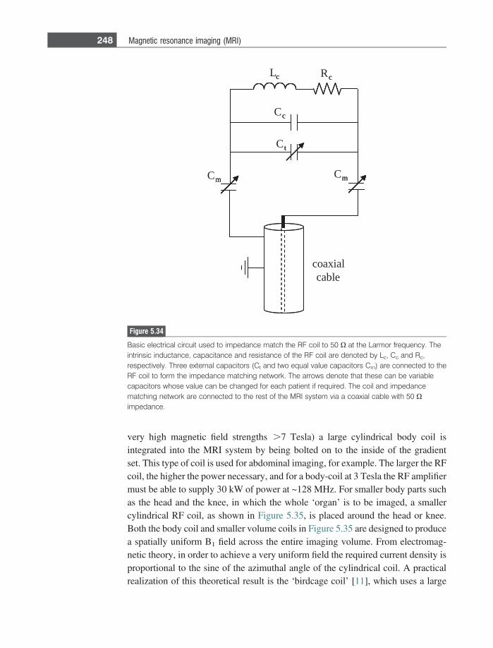
very high magnetic field strengths .7 Tesla) a large cylindrical body coil isintegrated into the MRI system by being bolted on to the inside of the gradientset. This type of coil is used for abdominal imaging, for example. The larger the RFcoil, the higher the power necessary, and for a body-coil at 3 Tesla the RF amplifiermust be able to supply 30 kW of power at ~128 MHz. For smaller body parts suchas the head and the knee, in which the whole ‘organ’ is to be imaged, a smallercylindrical RF coil, as shown in Figure 5.35, is placed around the head or knee.Both the body coil and smaller volume coils in Figure 5.35 are designed to producea spatially uniform B1 field across the entire imaging volume. From electromag-netic theory, in order to achieve a very uniform field the required current density isproportional to the sine of the azimuthal angle of the cylindrical coil. A practicalrealization of this theoretical result is the ‘birdcage coil’ [11], which uses a large
Lc Rc
Cm
Cc
Cm
Ct
coaxialcable
c c
m
c
m
t
Figure 5.34
Basic electrical circuit used to impedance match the RF coil to 50 X at the Larmor frequency. Theintrinsic inductance, capacitance and resistance of the RF coil are denoted by Lc, Cc and Rc,respectively. Three external capacitors (Ct and two equal value capacitors Cm) are connected to theRF coil to form the impedance matching network. The arrows denote that these can be variablecapacitors whose value can be changed for each patient if required. The coil and impedancematching network are connected to the rest of the MRI system via a coaxial cable with 50 Ximpedance.
248 Magnetic resonance imaging (MRI)
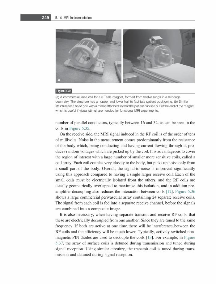
number of parallel conductors, typically between 16 and 32, as can be seen in thecoils in Figure 5.35.
On the receive side, the MRI signal induced in the RF coil is of the order of tensof millivolts. Noise in the measurement comes predominantly from the resistanceof the body which, being conducting and having current flowing through it, pro-duces random voltages which are picked up by the coil. It is advantageous to coverthe region of interest with a large number of smaller more sensitive coils, called acoil array. Each coil couples very closely to the body, but picks up noise only froma small part of the body. Overall, the signal-to-noise is improved significantlyusing this approach compared to having a single larger receive coil. Each of thesmall coils must be electrically isolated from the others, and the RF coils areusually geometrically overlapped to maximize this isolation, and in addition pre-amplifier decoupling also reduces the interaction between coils [12]. Figure 5.36shows a large commercial perivascular array containing 24 separate receive coils.The signal from each coil is fed into a separate receive channel, before the signalsare combined into a composite image.
It is also necessary, when having separate transmit and receive RF coils, thatthese are electrically decoupled from one another. Since they are tuned to the samefrequency, if both are active at one time there will be interference between theRF coils and the efficiency will be much lower. Typically, actively-switched non-magnetic PIN diodes are used to decouple the coils [13]. For example, in Figure5.37, the array of surface coils is detuned during transmission and tuned duringsignal reception. Using similar circuitry, the transmit coil is tuned during trans-mission and detuned during signal reception.
ba
Figure 5.35
(a) A commercial knee coil for a 3 Tesla magnet, formed from twelve rungs in a birdcagegeometry. The structure has an upper and lower half to facilitate patient positioning. (b) Similarstructure for a head coil, with a mirror attached so that the patient can see out of the end of the magnet,which is useful if visual stimuli are needed for functional MRI experiments.
249 5.14 MRI instrumentation
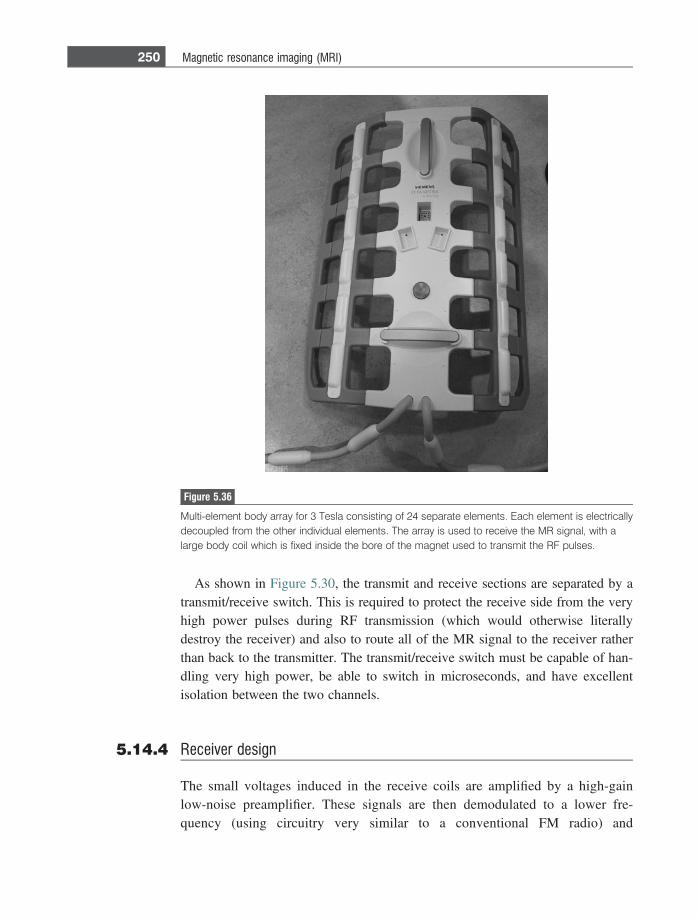
As shown in Figure 5.30, the transmit and receive sections are separated by atransmit/receive switch. This is required to protect the receive side from the veryhigh power pulses during RF transmission (which would otherwise literallydestroy the receiver) and also to route all of the MR signal to the receiver ratherthan back to the transmitter. The transmit/receive switch must be capable of han-dling very high power, be able to switch in microseconds, and have excellentisolation between the two channels.
5.14.4 Receiver design
The small voltages induced in the receive coils are amplified by a high-gainlow-noise preamplifier. These signals are then demodulated to a lower fre-quency (using circuitry very similar to a conventional FM radio) and
Figure 5.36
Multi-element body array for 3 Tesla consisting of 24 separate elements. Each element is electricallydecoupled from the other individual elements. The array is used to receive the MR signal, with alarge body coil which is fixed inside the bore of the magnet used to transmit the RF pulses.
250 Magnetic resonance imaging (MRI)
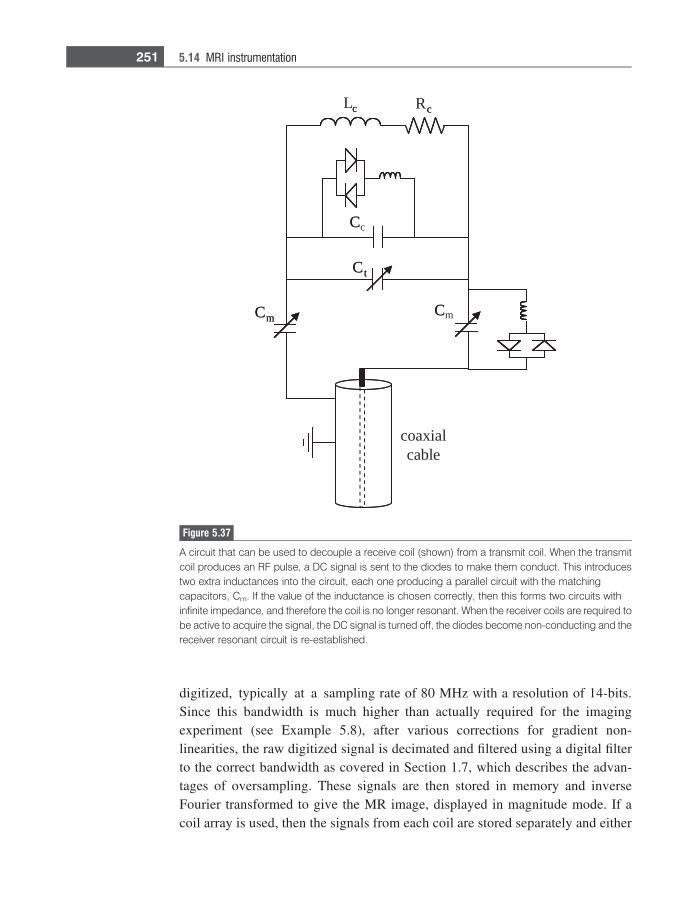
digitized, typically at a sampling rate of 80 MHz with a resolution of 14-bits.Since this bandwidth is much higher than actually required for the imagingexperiment (see Example 5.8), after various corrections for gradient non-linearities, the raw digitized signal is decimated and filtered using a digital filterto the correct bandwidth as covered in Section 1.7, which describes the advan-tages of oversampling. These signals are then stored in memory and inverseFourier transformed to give the MR image, displayed in magnitude mode. If acoil array is used, then the signals from each coil are stored separately and either
Lc Rc
Cm
Cc
Cm
Ct
coaxialcable
c c
Cm
C
C
Ct
Figure 5.37
A circuit that can be used to decouple a receive coil (shown) from a transmit coil. When the transmitcoil produces an RF pulse, a DC signal is sent to the diodes to make them conduct. This introducestwo extra inductances into the circuit, each one producing a parallel circuit with the matchingcapacitors, Cm. If the value of the inductance is chosen correctly, then this forms two circuits withinfinite impedance, and therefore the coil is no longer resonant. When the receiver coils are required tobe active to acquire the signal, the DC signal is turned off, the diodes become non-conducting and thereceiver resonant circuit is re-established.
251 5.14 MRI instrumentation
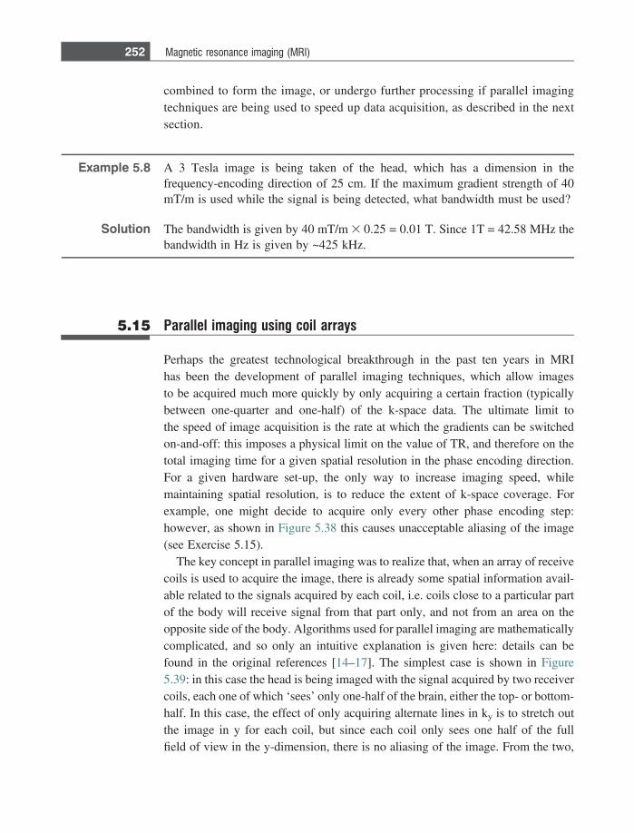
combined to form the image, or undergo further processing if parallel imagingtechniques are being used to speed up data acquisition, as described in the nextsection.
Example 5.8 A 3 Tesla image is being taken of the head, which has a dimension in thefrequency-encoding direction of 25 cm. If the maximum gradient strength of 40mT/m is used while the signal is being detected, what bandwidth must be used?
Solution The bandwidth is given by 40 mT/m 3 0.25 = 0.01 T. Since 1T = 42.58 MHz thebandwidth in Hz is given by ~425 kHz.
5.15 Parallel imaging using coil arrays
Perhaps the greatest technological breakthrough in the past ten years in MRIhas been the development of parallel imaging techniques, which allow imagesto be acquired much more quickly by only acquiring a certain fraction (typicallybetween one-quarter and one-half) of the k-space data. The ultimate limit tothe speed of image acquisition is the rate at which the gradients can be switchedon-and-off: this imposes a physical limit on the value of TR, and therefore on thetotal imaging time for a given spatial resolution in the phase encoding direction.For a given hardware set-up, the only way to increase imaging speed, whilemaintaining spatial resolution, is to reduce the extent of k-space coverage. Forexample, one might decide to acquire only every other phase encoding step:however, as shown in Figure 5.38 this causes unacceptable aliasing of the image(see Exercise 5.15).
The key concept in parallel imaging was to realize that, when an array of receivecoils is used to acquire the image, there is already some spatial information avail-able related to the signals acquired by each coil, i.e. coils close to a particular partof the body will receive signal from that part only, and not from an area on theopposite side of the body. Algorithms used for parallel imaging are mathematicallycomplicated, and so only an intuitive explanation is given here: details can befound in the original references [14–17]. The simplest case is shown in Figure5.39: in this case the head is being imaged with the signal acquired by two receivercoils, each one of which ‘sees’ only one-half of the brain, either the top- or bottom-half. In this case, the effect of only acquiring alternate lines in ky is to stretch outthe image in y for each coil, but since each coil only sees one half of the fullfield of view in the y-dimension, there is no aliasing of the image. From the two,
252 Magnetic resonance imaging (MRI)
non-overlapping stretched versions of the brain, it is very simple to add the imagestogether and rescale to produce a full image, acquired in half the time of a fullyencoded image.
The trade-off in parallel imaging is between the reduced data acquisition timeand a reduced SNR. However, in many clinical situations the limiting factor is notthe SNR but the time required to acquire an image. One example is abdominalimaging of the liver, in which it is important to be able to acquire the entire imagewithin a single breath-hold to avoid image artifacts from motion. Clinical patientsmay only be able to hold their breath for less than ten seconds, and so rapid dataacquisition is needed. An example is shown in Figure 5.40, in which dynamicswallowing of a water bolus is acquired in real-time using parallel imaging, whichallowed a four-fold decrease in imaging time.
kx
ky
kx
ky
kx
ky
x
ky
x
y
kx
ky
x
ky
x
y
a b
Figure 5.38
(a) A full k-space matrix (top) gives an unaliased image (bottom) provided that the Dkx and Dky
increments are correctly set. (b) If data acquisition speed is increased by a factor of 2 by acquiring onlyalternate ky lines, then the Dky is doubled, the image field-of-view in the y-dimension is halved, and theimage is aliased along the y-dimension.
253 5.15 Parallel imaging using coil arrays
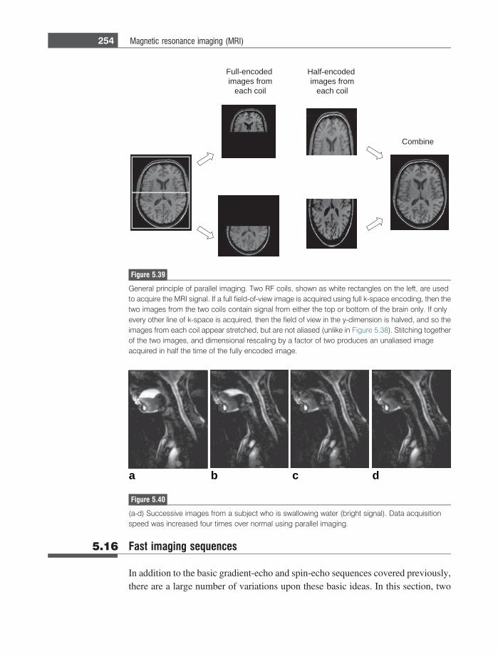
5.16 Fast imaging sequences
In addition to the basic gradient-echo and spin-echo sequences covered previously,there are a large number of variations upon these basic ideas. In this section, two
dedocne-lluF
morf segami
lioc hcae
dedocne-flaH
morf segami
lioc hcae
enibmoC
Figure 5.39
General principle of parallel imaging. Two RF coils, shown as white rectangles on the left, are usedto acquire the MRI signal. If a full field-of-view image is acquired using full k-space encoding, then thetwo images from the two coils contain signal from either the top or bottom of the brain only. If onlyevery other line of k-space is acquired, then the field of view in the y-dimension is halved, and so theimages from each coil appear stretched, but are not aliased (unlike in Figure 5.38). Stitching togetherof the two images, and dimensional rescaling by a factor of two produces an unaliased imageacquired in half the time of the fully encoded image.
a b c d
Figure 5.40
(a-d) Successive images from a subject who is swallowing water (bright signal). Data acquisitionspeed was increased four times over normal using parallel imaging.
254 Magnetic resonance imaging (MRI)
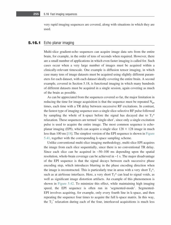
very rapid imaging sequences are covered, along with situations in which they areused.
5.16.1 Echo planar imaging
Multi-slice gradient-echo sequences can acquire image data sets from the entirebrain, for example, in the order of tens of seconds when required. However, thereare a small number of applications in which even faster imaging is called for. Suchcases occur when a very large number of images must be acquired within aclinically-relevant timescale. One example is diffusion tensor imaging, in whichcase many tens of image datasets must be acquired using slightly different param-eters for each dataset, with each dataset ideally covering the entire brain. A secondexample, covered in Section 5.18, is functional imaging in which many hundredsof different datasets must be acquired in a single session, again covering as muchof the brain as possible.
As can be appreciated from the sequences covered so far, the major limitation inreducing the time for image acquisition is that the sequence must be repeated Npe
times, each time with a TR delay between successive RF excitations. In contrast,the fastest type of imaging sequence uses a single slice-selective RF pulse followedby sampling the whole of k-space before the signal has decayed due to T2*relaxation. These sequences are termed ‘single-shot’, since only a single excitationpulse is used to acquire the entire image. The most common sequence is echo-planar imaging (EPI), which can acquire a single slice 128 3 128 image in muchless than 100 ms [18]. The simplest version of the EPI sequence is shown in Figure5.41, together with the corresponding k-space sampling scheme.
Unlike conventional multi-slice imaging methodology, multi-slice EPI acquiresthe image from each slice sequentially, since there is no conventional TR delay.Since each slice can be acquired in ~50–100 ms depending upon the spatialresolution, whole-brain coverage can be achieved in ~1 s. The major disadvantageof the EPI sequence is that the signal decays between each successive phaseencoding step, which introduces blurring in the phase encoding direction whenthe image is reconstructed. This is particularly true in areas with a very short T2*,such as at air/tissue interfaces. Here, a very short T2* can lead to signal voids, aswell as significant image distortion artifacts. An example of this phenomenon isshown in Figure 5.42. To minimize this effect, while maintaining high imagingspeed, the EPI sequence is often run in ‘segmented-mode’. Segmented-EPI involves acquiring, for example, only every fourth line in k-space, and thenrepeating the sequence four times to acquire the full k-space matrix. In this way,the T2
* relaxation during each of the four, interleaved acquisitions is much less
255 5.16 Fast imaging sequences
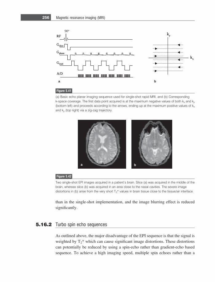
than in the single-shot implementation, and the image blurring effect is reducedsignificantly.
5.16.2 Turbo spin echo sequences
As outlined above, the major disadvantage of the EPI sequence is that the signal isweighted by T2* which can cause significant image distortions. These distortionscan potentially be reduced by using a spin-echo rather than gradient-echo basedsequence. To achieve a high imaging speed, multiple spin echoes rather than a
RF
Gslice
Gphase
Gread
A/D
90o
kx
kyRF
Gslice
Gphase
Gread
A/D
kx
ky
a b
Figure 5.41
(a) Basic echo planar imaging sequence used for single-shot rapid MRI, and (b) Correspondingk-space coverage. The first data point acquired is at the maximum negative values of both kx and ky
(bottom left) and proceeds according to the arrows, ending up at the maximum positive values of kx
and ky (top right) via a zig-zag trajectory.
a b
Figure 5.42
Two single-shot EPI images acquired in a patient’s brain. Slice (a) was acquired in the middle of thebrain, whereas slice (b) was acquired in an area close to the nasal cavities. The severe imagedistortions in (b) arise from the very short T2* values in brain tissue close to the tissue/air interface.
256 Magnetic resonance imaging (MRI)
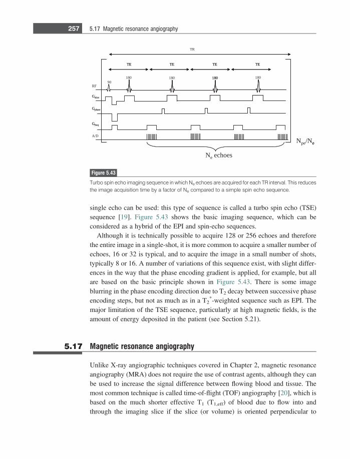
single echo can be used: this type of sequence is called a turbo spin echo (TSE)sequence [19]. Figure 5.43 shows the basic imaging sequence, which can beconsidered as a hybrid of the EPI and spin-echo sequences.
Although it is technically possible to acquire 128 or 256 echoes and thereforethe entire image in a single-shot, it is more common to acquire a smaller number ofechoes, 16 or 32 is typical, and to acquire the image in a small number of shots,typically 8 or 16. A number of variations of this sequence exist, with slight differ-ences in the way that the phase encoding gradient is applied, for example, but allare based on the basic principle shown in Figure 5.43. There is some imageblurring in the phase encoding direction due to T2 decay between successive phaseencoding steps, but not as much as in a T2
*-weighted sequence such as EPI. Themajor limitation of the TSE sequence, particularly at high magnetic fields, is theamount of energy deposited in the patient (see Section 5.21).
5.17 Magnetic resonance angiography
Unlike X-ray angiographic techniques covered in Chapter 2, magnetic resonanceangiography (MRA) does not require the use of contrast agents, although they canbe used to increase the signal difference between flowing blood and tissue. Themost common technique is called time-of-flight (TOF) angiography [20], which isbased on the much shorter effective T1 (T1,eff) of blood due to flow into andthrough the imaging slice if the slice (or volume) is oriented perpendicular to
TE
TR
90180
RF
Gfreq
Gphase
Gslice
A/DNpe/Ne
180 180 180
TE TE TE
Ne echoes
TE
Gfreq
Gphase
Gslice
e
180
TE TE TE
Figure 5.43
Turbo spin echo imaging sequence in which Ne echoes are acquired for each TR interval. This reducesthe image acquisition time by a factor of Ne compared to a simple spin echo sequence.
257 5.17 Magnetic resonance angiography
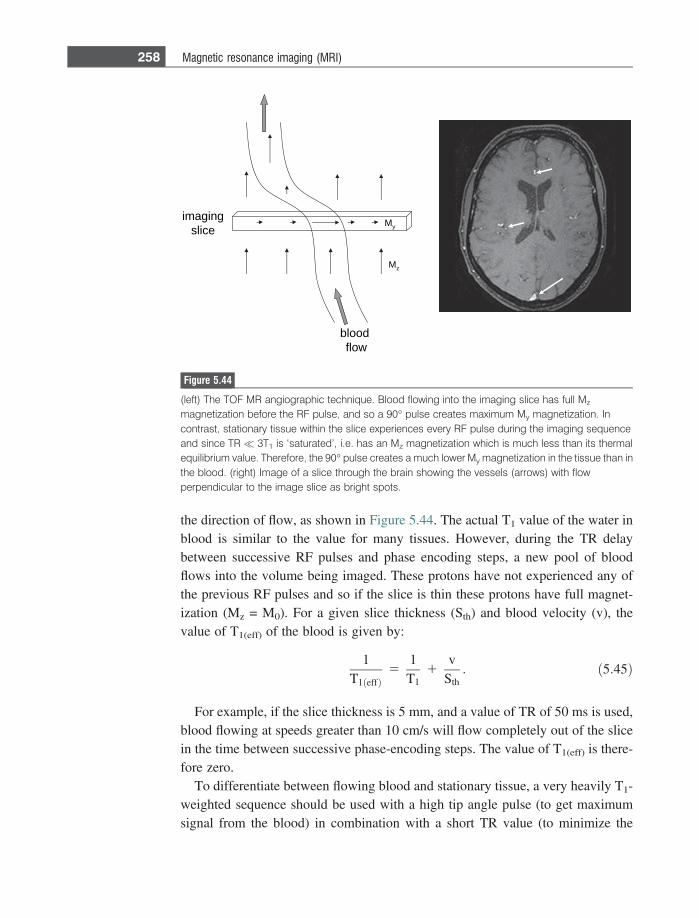
the direction of flow, as shown in Figure 5.44. The actual T1 value of the water inblood is similar to the value for many tissues. However, during the TR delaybetween successive RF pulses and phase encoding steps, a new pool of bloodflows into the volume being imaged. These protons have not experienced any ofthe previous RF pulses and so if the slice is thin these protons have full magnet-ization (Mz = M0). For a given slice thickness (Sth) and blood velocity (v), thevalue of T1(eff) of the blood is given by:
1T1ðeffÞ
51T1
1v
Sth: ð5:45Þ
For example, if the slice thickness is 5 mm, and a value of TR of 50 ms is used,blood flowing at speeds greater than 10 cm/s will flow completely out of the slicein the time between successive phase-encoding steps. The value of T1(eff) is there-fore zero.
To differentiate between flowing blood and stationary tissue, a very heavily T1-weighted sequence should be used with a high tip angle pulse (to get maximumsignal from the blood) in combination with a short TR value (to minimize the
gnigami
ecils
doolb
wolf
Mz
My
Figure 5.44
(left) The TOF MR angiographic technique. Blood flowing into the imaging slice has full Mz
magnetization before the RF pulse, and so a 90� pulse creates maximum My magnetization. Incontrast, stationary tissue within the slice experiences every RF pulse during the imaging sequenceand since TR� 3T1 is ‘saturated’, i.e. has an Mz magnetization which is much less than its thermalequilibrium value. Therefore, the 90� pulse creates a much lower My magnetization in the tissue than inthe blood. (right) Image of a slice through the brain showing the vessels (arrows) with flowperpendicular to the image slice as bright spots.
258 Magnetic resonance imaging (MRI)
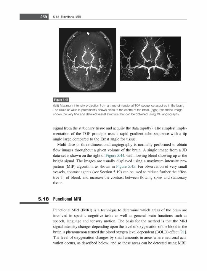
signal from the stationary tissue and acquire the data rapidly). The simplest imple-mentation of the TOF principle uses a rapid gradient-echo sequence with a tipangle large compared to the Ernst angle for tissue.
Multi-slice or three-dimensional angiography is normally performed to obtainflow images throughout a given volume of the brain. A single image from a 3Ddata-set is shown on the right of Figure 5.44, with flowing blood showing up as thebright signal. The images are usually displayed using a maximum intensity pro-jection (MIP) algorithm, as shown in Figure 5.45. For observation of very smallvessels, contrast agents (see Section 5.19) can be used to reduce further the effec-tive T1 of blood, and increase the contrast between flowing spins and stationarytissue.
5.18 Functional MRI
Functional MRI (fMRI) is a technique to determine which areas of the brain areinvolved in specific cognitive tasks as well as general brain functions such asspeech, language and sensory motion. The basis for the method is that the MRIsignal intensity changes depending upon the level of oxygenation of the blood in thebrain, a phenomenon termed the blood oxygen level dependent (BOLD) effect [21].The level of oxygenation changes by small amounts in areas where neuronal acti-vation occurs, as described below, and so these areas can be detected using MRI.
Figure 5.45
(left) Maximum intensity projection from a three-dimensional TOF sequence acquired in the brain.The circle-of-Willis is prominently shown close to the centre of the brain. (right) Expanded imageshows the very fine and detailed vessel structure that can be obtained using MR angiography.
259 5.18 Functional MRI
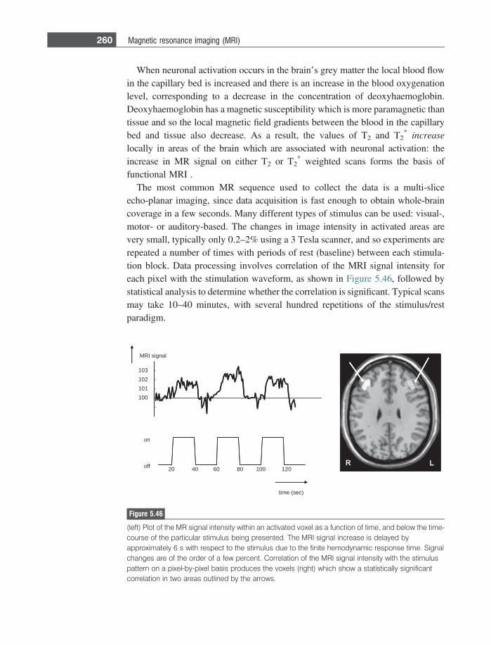
When neuronal activation occurs in the brain’s grey matter the local blood flowin the capillary bed is increased and there is an increase in the blood oxygenationlevel, corresponding to a decrease in the concentration of deoxyhaemoglobin.Deoxyhaemoglobin has a magnetic susceptibility which is more paramagnetic thantissue and so the local magnetic field gradients between the blood in the capillarybed and tissue also decrease. As a result, the values of T2 and T2
* increaselocally in areas of the brain which are associated with neuronal activation: theincrease in MR signal on either T2 or T2
* weighted scans forms the basis offunctional MRI .
The most common MR sequence used to collect the data is a multi-sliceecho-planar imaging, since data acquisition is fast enough to obtain whole-braincoverage in a few seconds. Many different types of stimulus can be used: visual-,motor- or auditory-based. The changes in image intensity in activated areas arevery small, typically only 0.2–2% using a 3 Tesla scanner, and so experiments arerepeated a number of times with periods of rest (baseline) between each stimula-tion block. Data processing involves correlation of the MRI signal intensity foreach pixel with the stimulation waveform, as shown in Figure 5.46, followed bystatistical analysis to determine whether the correlation is significant. Typical scansmay take 10–40 minutes, with several hundred repetitions of the stimulus/restparadigm.
100
101
102
103
20 40 60 80 100 120 off
on
time (sec)
MRI signal
Figure 5.46
(left) Plot of the MR signal intensity within an activated voxel as a function of time, and below the time-course of the particular stimulus being presented. The MRI signal increase is delayed byapproximately 6 s with respect to the stimulus due to the finite hemodynamic response time. Signalchanges are of the order of a few percent. Correlation of the MRI signal intensity with the stimuluspattern on a pixel-by-pixel basis produces the voxels (right) which show a statistically significantcorrelation in two areas outlined by the arrows.
260 Magnetic resonance imaging (MRI)
Although fMRI is currently used more for research than routine clinical use, it isincreasingly being used in a number of presurgical planning studies. Here, theexact surgical ‘route’ for removing, for example, a tumour from the brain can beplanned by avoiding areas which have been determined to be involved in criticalcognitive tasks such as language recognition and motor processes.
5.19 MRI contrast agents
In many clinical scans, there is sufficient contrast-to-noise on the appropriate T1-,T2- or proton density-weighted image to distinguish diseased from healthy tissue.However, in certain cases such as the detection of very small lesions, where partialvolume effects occur within the slice, the CNR may be too low for a definitivediagnosis. In this case, MRI contrast agents can be used to increase the CNRbetween healthy and diseased tissue. There are two basic classes of MRI contrastagent: paramagnetic and superparamagnetic, also called positive and negativeagents, respectively. In addition to lesion detection, positive agents are also oftenused in combination with TOF angiography.
5.19.1 Positive contrast agents
Paramagnetic contrast agents shorten the T1 of the tissue in which they accumulate,and are therefore referred to clinically as positive contrast agents since theyincrease the MRI signal on T1-weighted scans. There are currently several differentagents (which go by trade names such as Omniscan, Prohance and Magnevist)which are approved worldwide for clinical use. The differences between the var-ious agents are in the ionicity and osmolarity, similar to X-ray contrast agentscovered in Chapter 2. All the agents are based on a central gadolinium ion, which issurrounded by a particular chemical chelate, as shown in Figure 5.47. Neither thegadolinium nor the chelate produces an MR signal directly, but the chelatedmolecule is visualized via its effect on water molecules in the tissue in whichthe contrast agent accumulates. The Gd3+ ion has seven unpaired electrons, andthe interaction between water protons and these electrons produces a very efficientT1 relaxation and so reduces the T1 time of the tissue. The agents are designed sothat there is one empty binding site to the Gd ion which is not occupied by thechelate structure. This means that a water molecule can temporarily bind to thissite, undergo very rapid T1 relaxation and then be released to be succeeded by asecond water molecule, and so on. This mechanism is referred to as ‘inner sphererelaxation’. A second way in which water molecules can have their T1 relaxationtime reduced is simply by interacting with the unpaired Gd electrons at a distance,
261 5.19 MRI contrast agents
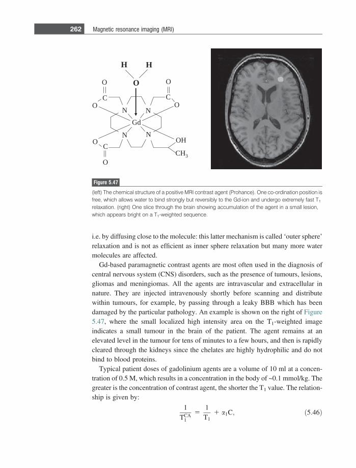
i.e. by diffusing close to the molecule: this latter mechanism is called ‘outer sphere’relaxation and is not as efficient as inner sphere relaxation but many more watermolecules are affected.
Gd-based paramagnetic contrast agents are most often used in the diagnosis ofcentral nervous system (CNS) disorders, such as the presence of tumours, lesions,gliomas and meningiomas. All the agents are intravascular and extracellular innature. They are injected intravenously shortly before scanning and distributewithin tumours, for example, by passing through a leaky BBB which has beendamaged by the particular pathology. An example is shown on the right of Figure5.47, where the small localized high intensity area on the T1-weighted imageindicates a small tumour in the brain of the patient. The agent remains at anelevated level in the tumour for tens of minutes to a few hours, and then is rapidlycleared through the kidneys since the chelates are highly hydrophilic and do notbind to blood proteins.
Typical patient doses of gadolinium agents are a volume of 10 ml at a concen-tration of 0.5 M, which results in a concentration in the body of ~0.1 mmol/kg. Thegreater is the concentration of contrast agent, the shorter the T1 value. The relation-ship is given by:
1
TCA1
51
T11 a1C; ð5:46Þ
dG
N
N N
N
O
HO
HC 3
O
OC
O
O
O
C
C
HH
O
Figure 5.47
(left) The chemical structure of a positive MRI contrast agent (Prohance). One co-ordination position isfree, which allows water to bind strongly but reversibly to the Gd-ion and undergo extremely fast T1
relaxation. (right) One slice through the brain showing accumulation of the agent in a small lesion,which appears bright on a T1-weighted sequence.
262 Magnetic resonance imaging (MRI)
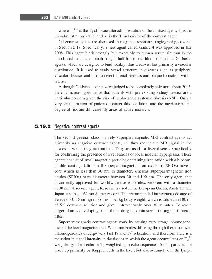
where T1CA is the T1 of tissue after administration of the contrast agent, T1 is the
pre-adminstration value, and a1 is the T1-relaxivity of the contrast agent.Gd contrast agents are also used in magnetic resonance angiography, covered
in Section 5.17. Specifically, a new agent called Gadovist was approved in late2008. This agent binds strongly but reversibly to human serum albumin in theblood, and so has a much longer half-life in the blood than other Gd-basedagents, which are designed to bind weakly: thus Gadovist has primarily a vasculardistribution. It is used to study vessel structure in diseases such as peripheralvascular disease, and also to detect arterial stenosis and plaque formation withinarteries.
Although Gd-based agents were judged to be completely safe until about 2005,there is increasing evidence that patients with pre-existing kidney disease are aparticular concern given the risk of nephrogenic systemic fibrosis (NSF). Only avery small fraction of patients contract this condition, and the mechanism anddegree of risk are still currently areas of active research.
5.19.2 Negative contrast agents
The second general class, namely superparamagnetic MRI contrast agents actprimarily as negative contrast agents, i.e. they reduce the MR signal in thetissues in which they accumulate. They are used for liver disease, specificallyfor confirming the presence of liver lesions or focal nodular hyperplasia. Theseagents consist of small magnetic particles containing iron oxide with a biocom-patible coating. Ultra-small superparamagnetic iron oxides (USPIOs) have acore which is less than 30 nm in diameter, whereas superparamagnetic ironoxides (SPIOs) have diameters between 30 and 100 nm. The only agent thatis currently approved for worldwide use is Feridex/Endorem with a diameter~100 nm. A second agent, Resovist is used in the European Union, Australia andJapan, and has a 62 nm diameter core. The recommended intravenous dosage ofFeridex is 0.56 milligrams of iron per kg body weight, which is diluted in 100 mlof 5% dextrose solution and given intravenously over 30 minutes. To avoidlarger clumps developing, the diluted drug is administered through a 5 micronfilter.
Superparamagnetic contrast agents work by causing very strong inhomogene-ities in the local magnetic field. Water molecules diffusing through these localizedinhomogeneities undergo very fast T2 and T2
* relaxation, and therefore there is areduction in signal intensity in the tissues in which the agent accumulates on T2
*-weighted gradient-echo or T2-weighted spin-echo sequences. Small particles aretaken up primarily by Kuppfer cells in the liver, but also accumulate in the lymph
263 5.19 MRI contrast agents
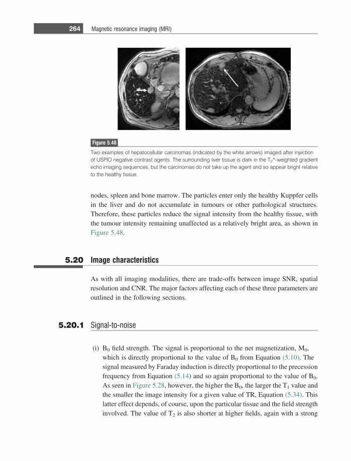
nodes, spleen and bone marrow. The particles enter only the healthy Kuppfer cellsin the liver and do not accumulate in tumours or other pathological structures.Therefore, these particles reduce the signal intensity from the healthy tissue, withthe tumour intensity remaining unaffected as a relatively bright area, as shown inFigure 5.48.
5.20 Image characteristics
As with all imaging modalities, there are trade-offs between image SNR, spatialresolution and CNR. The major factors affecting each of these three parameters areoutlined in the following sections.
5.20.1 Signal-to-noise
(i) B0 field strength. The signal is proportional to the net magnetization, M0,which is directly proportional to the value of B0 from Equation (5.10). Thesignal measured by Faraday induction is directly proportional to the precessionfrequency from Equation (5.14) and so again proportional to the value of B0.As seen in Figure 5.28, however, the higher the B0, the larger the T1 value andthe smaller the image intensity for a given value of TR, Equation (5.34). Thislatter effect depends, of course, upon the particular tissue and the field strengthinvolved. The value of T2 is also shorter at higher fields, again with a strong
Figure 5.48
Two examples of hepatocellular carcinomas (indicated by the white arrows) imaged after injectionof USPIO negative contrast agents. The surrounding liver tissue is dark in the T2*-weighted gradientecho imaging sequences, but the carcinomas do not take up the agent and so appear bright relativeto the healthy tissue.
264 Magnetic resonance imaging (MRI)
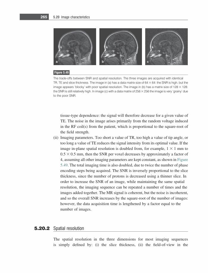
tissue-type dependence: the signal will therefore decrease for a given value ofTE. The noise in the image arises primarily from the random voltage inducedin the RF coil(s) from the patient, which is proportional to the square-root ofthe field strength.
(ii) Imaging parameters. Too short a value of TR, too high a value of tip angle, ortoo long a value of TE reduces the signal intensity from its optimal value. If theimage in-plane spatial resolution is doubled from, for example, 1 3 1 mm to0.5 3 0.5 mm, then the SNR per voxel decreases by approximately a factor of4, assuming all other imaging parameters are kept constant, as shown in Figure5.49. The total imaging time is also doubled, due to twice the number of phaseencoding steps being acquired. The SNR is inversely proportional to the slicethickness, since the number of protons is decreased using a thinner slice. Inorder to increase the SNR of an image, while maintaining the same spatialresolution, the imaging sequence can be repeated a number of times and theimages added together. The MR signal is coherent, but the noise is incoherent,and so the overall SNR increases by the square-root of the number of images:however, the data acquisition time is lengthened by a factor equal to thenumber of images.
5.20.2 Spatial resolution
The spatial resolution in the three dimensions for most imaging sequencesis simply defined by: (i) the slice thickness, (ii) the field-of-view in the
a b c
Figure 5.49
The trade-offs between SNR and spatial resolution. The three images are acquired with identicalTR, TE and slice thickness. The image in (a) has a data matrix size of 64 3 64: the SNR is high, but theimage appears ‘blocky’ with poor spatial resolution. The image in (b) has a matrix size of 128 3 128:the SNR is still relatively high. In image (c) with a data matrix of 256 3 256 the image is very ‘grainy’ dueto the poor SNR.
265 5.20 Image characteristics
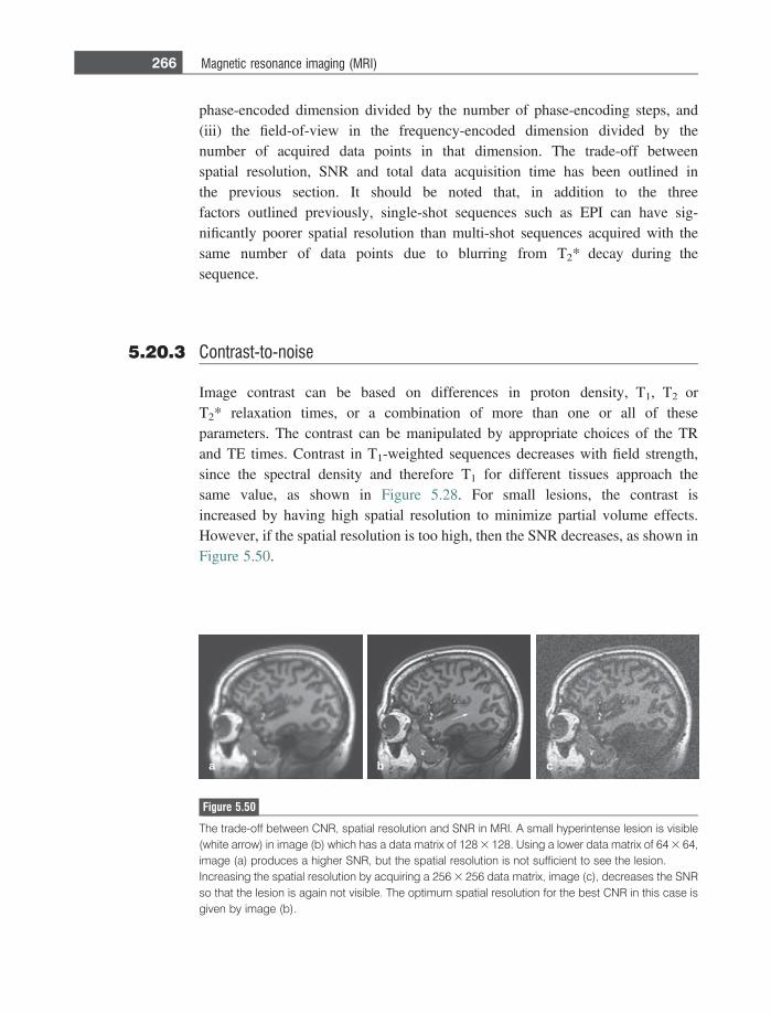
phase-encoded dimension divided by the number of phase-encoding steps, and(iii) the field-of-view in the frequency-encoded dimension divided by thenumber of acquired data points in that dimension. The trade-off betweenspatial resolution, SNR and total data acquisition time has been outlined inthe previous section. It should be noted that, in addition to the threefactors outlined previously, single-shot sequences such as EPI can have sig-nificantly poorer spatial resolution than multi-shot sequences acquired with thesame number of data points due to blurring from T2* decay during thesequence.
5.20.3 Contrast-to-noise
Image contrast can be based on differences in proton density, T1, T2 orT2* relaxation times, or a combination of more than one or all of theseparameters. The contrast can be manipulated by appropriate choices of the TRand TE times. Contrast in T1-weighted sequences decreases with field strength,since the spectral density and therefore T1 for different tissues approach thesame value, as shown in Figure 5.28. For small lesions, the contrast isincreased by having high spatial resolution to minimize partial volume effects.However, if the spatial resolution is too high, then the SNR decreases, as shown inFigure 5.50.
a b c
Figure 5.50
The trade-off between CNR, spatial resolution and SNR in MRI. A small hyperintense lesion is visible(white arrow) in image (b) which has a data matrix of 128 3 128. Using a lower data matrix of 64 3 64,image (a) produces a higher SNR, but the spatial resolution is not sufficient to see the lesion.Increasing the spatial resolution by acquiring a 256 3 256 data matrix, image (c), decreases the SNRso that the lesion is again not visible. The optimum spatial resolution for the best CNR in this case isgiven by image (b).
266 Magnetic resonance imaging (MRI)
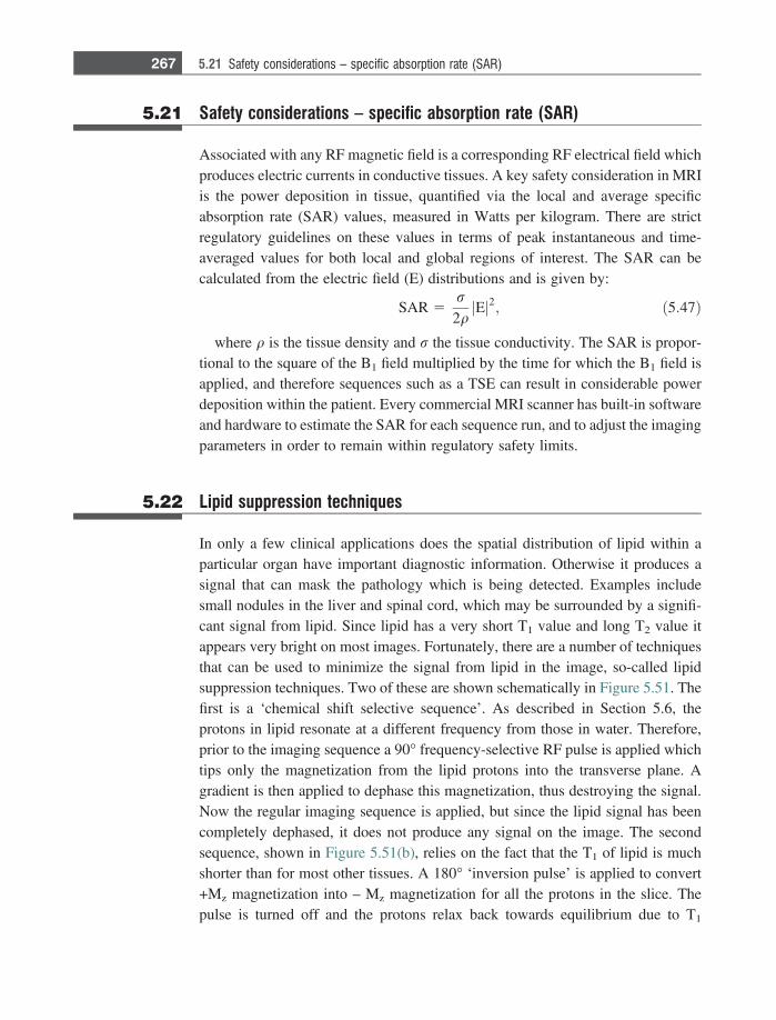
5.21 Safety considerations – specific absorption rate (SAR)
Associated with any RF magnetic field is a corresponding RF electrical field whichproduces electric currents in conductive tissues. A key safety consideration in MRIis the power deposition in tissue, quantified via the local and average specificabsorption rate (SAR) values, measured in Watts per kilogram. There are strictregulatory guidelines on these values in terms of peak instantaneous and time-averaged values for both local and global regions of interest. The SAR can becalculated from the electric field (E) distributions and is given by:
SAR 5r2q
Ej j2; ð5:47Þ
where q is the tissue density and r the tissue conductivity. The SAR is propor-tional to the square of the B1 field multiplied by the time for which the B1 field isapplied, and therefore sequences such as a TSE can result in considerable powerdeposition within the patient. Every commercial MRI scanner has built-in softwareand hardware to estimate the SAR for each sequence run, and to adjust the imagingparameters in order to remain within regulatory safety limits.
5.22 Lipid suppression techniques
In only a few clinical applications does the spatial distribution of lipid within aparticular organ have important diagnostic information. Otherwise it produces asignal that can mask the pathology which is being detected. Examples includesmall nodules in the liver and spinal cord, which may be surrounded by a signifi-cant signal from lipid. Since lipid has a very short T1 value and long T2 value itappears very bright on most images. Fortunately, there are a number of techniquesthat can be used to minimize the signal from lipid in the image, so-called lipidsuppression techniques. Two of these are shown schematically in Figure 5.51. Thefirst is a ‘chemical shift selective sequence’. As described in Section 5.6, theprotons in lipid resonate at a different frequency from those in water. Therefore,prior to the imaging sequence a 90� frequency-selective RF pulse is applied whichtips only the magnetization from the lipid protons into the transverse plane. Agradient is then applied to dephase this magnetization, thus destroying the signal.Now the regular imaging sequence is applied, but since the lipid signal has beencompletely dephased, it does not produce any signal on the image. The secondsequence, shown in Figure 5.51(b), relies on the fact that the T1 of lipid is muchshorter than for most other tissues. A 180� ‘inversion pulse’ is applied to convert+Mz magnetization into – Mz magnetization for all the protons in the slice. Thepulse is turned off and the protons relax back towards equilibrium due to T1
267 5.21 Safety considerations – specific absorption rate (SAR)
relaxation. At a specific time, termed the inversion time (TI), after the 180� pulse,the imaging sequence is started. The inversion time is chosen specifically so thatthe protons in lipid have relaxed back to a value of Mz = 0. When the imagingsequence is run, therefore, the slice selective pulse produces no transverse magnet-ization from the lipid and therefore no signal in the image. These lipid-suppressionsequences are called ‘inversion recovery’ sequences, with the most common clin-ical acronym being short time inversion recovery (STIR).
5.23 Clinical applications
Almost all parts of the body are imaged in the clinical setting: the brain and spinalcord, the entire musculoskeletal system (shoulder, knee, ankle, and hand), MRmammography, body imaging of the liver, kidneys, urinary tract and prostate, andcardiological applications looking at heart disease. The following applicationsrepresent only a small fraction of the total spectrum of clinical protocols.
5.23.1 Neurological applications
MRI can be used to diagnose both acute and chronic neurological diseases, and isthe imaging method of choice for intracranial mass lesions such as tumours, with
180o
Npe
RF
Gphase
A/D
Gslice
Gfreq
TI
imagingsequence
90o
Npe
RF
Gphase
A/D
Gslice
Gfreq
imaging
0,lipid
180o
Npe
RF
TI
90o
Npe
RF
A/D
freq
sequence
o
Npe
o90o
Npe
90o
ω 0,lipid
Figure 5.51
(a) Lipid saturation using frequency-selective excitation. The RF pulse tips only lipid protons intothe transverse plane: the magnetization is then rapidly dephased using ‘crusher’ gradients. Theimaging sequence then gives a signal only from the protons in tissue water. (b) An alternative methodfor lipid suppression. After the 180� pulse, an inversion delay (TI) is used, with the value chosen so thatthe lipid signal has zero longitudinal magnetization due to T1 relaxation, at which time the imagingsequence begins.
268 Magnetic resonance imaging (MRI)
the majority of imaging protocols involving administration of a positive contrastagent.
Many pathological conditions in the brain, such as vasogenic or cytotoxicoedema, result in increased water content, which gives a high signal intensity onT2-weighted sequences. Oedema is easily seen on T2-weighted sequences, and hasdifferent causes. Interstitial oedema arises from different forms of hydrocephalus,vasogenic oedema arises from breakdown of the BBB in primary and metastatictumours, and cytotoxic oedema is associated with ischemia.
Tumours located outside the brain (extra-axial tumours), examples of which aremeningioma, lymphoma, and schwannoma, are usually benign and after injectionof the contrast agent they enhance because of the tumour vascularity. Since they areoutside the brain they do not possess a BBB. Intra-axial tumours, such as astro-cytoma and glioblastomas, originate within the brain. These also enhance with Gdadministration, with high grade tumours generally enhancing more than low grade.
Stroke arises from large vessel occlusion. The cellular sodium/potassium pumpfails, leading to cytotoxic oedema. Thrombolytic therapy must be used within thefirst few hours after stroke and so early detection is key. Early cytotoxic oedemacan be detected using diffusion-weighted MRI which is very sensitive to cellswelling. About 20% of strokes come from occlusion of small arteries branchingfrom the major cerebral arteries, and can be visualized as small round lesions in T2-weighted scans, as well as showing enhancement on contrast agent administrationdue to disruption of the BBB.
Chronic diseases can either be characterized by specific features such as whitematter lesions, in multiple sclerosis for example as shown in Figure 5.52, or morediffuse areas of low intensity which indicate long-term accumulation of iron inareas such as the putamen, a characteristic of Huntington’s and Alzheimer’s dis-ease. Diagnosis in the latter cases is more difficult than for specific pathologies,since there are a number of other diseases which can lead to similar chronic events,and indeed the normal ageing process results in non-specific white-matter lesionsas well as increased iron deposition.
5.23.2 Body applications
Both diffuse and focal liver diseases can be diagnosed using MRI. Scans arenormally acquired during a single breath-hold of 10–20 s to avoid image artifactsfrom respiration. MRI is particularly useful for diagnosing lesions in fatty livers,since these can be obscured in ultrasound and CT. Lesions such as hepaticadenoma enhance strongly after positive contrast administration. Cirrhosis of theliver involves fibrosis which is irreversible, and atrophy in the different lobes is
269 5.23 Clinical applications
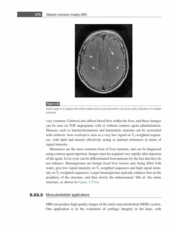
very common. Cirrhosis also affects blood flow within the liver, and these changescan be seen on TOF angiograms with or without contrast agent administration.Diseases such as haemochromatosis and haemolytic anaemia can be associatedwith cirrhosis. Iron overload is seen as a very low signal on T2-weighted sequen-ces, with lipid and muscle effectively acting as internal references in terms ofsignal intensity.
Metastases are the most common form of liver tumours, and can be diagnosedusing contrast agent injection. Images must be acquired very rapidly after injectionof the agent. Liver cysts can be differentiated from tumours by the fact that they donot enhance. Hemangiomas are benign focal liver lesions and, being filled withwater, give low signal intensity on T1-weighted sequences and high signal inten-sity on T2-weighted sequences. Larger hemangiomas typically enhance first on theperiphery of the structure, and then slowly the enhancement ‘fills in’ the entirestructure, as shown in Figure 5.53(b).
5.23.3 Musculoskeletal applications
MRI can produce high quality images of the entire musculoskeletal (MSK) system.One application is in the evaluation of cartilage integrity in the knee, with
Figure 5.52
Axial image of a subject with white matter lesions (arrows) which can be an early indication of multiplesclerosis.
270 Magnetic resonance imaging (MRI)
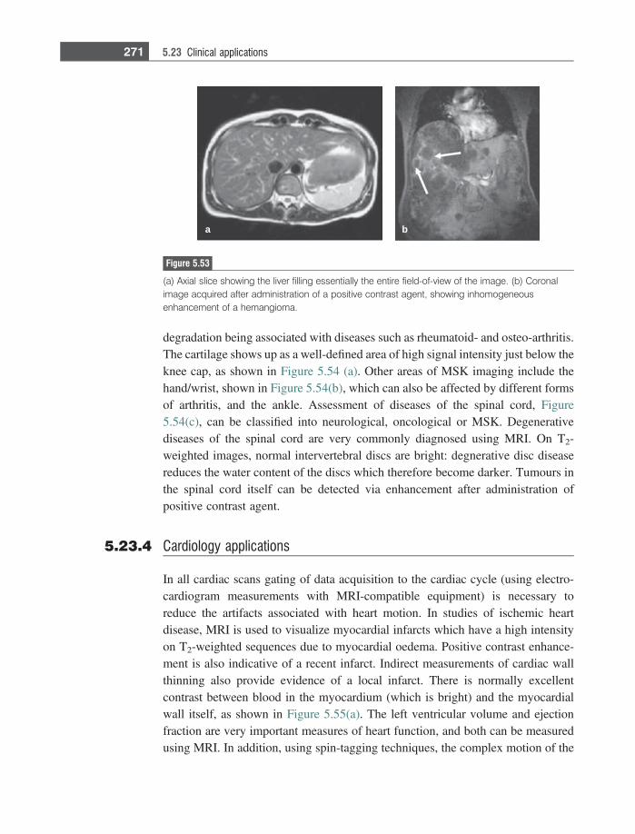
degradation being associated with diseases such as rheumatoid- and osteo-arthritis.The cartilage shows up as a well-defined area of high signal intensity just below theknee cap, as shown in Figure 5.54 (a). Other areas of MSK imaging include thehand/wrist, shown in Figure 5.54(b), which can also be affected by different formsof arthritis, and the ankle. Assessment of diseases of the spinal cord, Figure5.54(c), can be classified into neurological, oncological or MSK. Degenerativediseases of the spinal cord are very commonly diagnosed using MRI. On T2-weighted images, normal intervertebral discs are bright: degnerative disc diseasereduces the water content of the discs which therefore become darker. Tumours inthe spinal cord itself can be detected via enhancement after administration ofpositive contrast agent.
5.23.4 Cardiology applications
In all cardiac scans gating of data acquisition to the cardiac cycle (using electro-cardiogram measurements with MRI-compatible equipment) is necessary toreduce the artifacts associated with heart motion. In studies of ischemic heartdisease, MRI is used to visualize myocardial infarcts which have a high intensityon T2-weighted sequences due to myocardial oedema. Positive contrast enhance-ment is also indicative of a recent infarct. Indirect measurements of cardiac wallthinning also provide evidence of a local infarct. There is normally excellentcontrast between blood in the myocardium (which is bright) and the myocardialwall itself, as shown in Figure 5.55(a). The left ventricular volume and ejectionfraction are very important measures of heart function, and both can be measuredusing MRI. In addition, using spin-tagging techniques, the complex motion of the
a b
Figure 5.53
(a) Axial slice showing the liver filling essentially the entire field-of-view of the image. (b) Coronalimage acquired after administration of a positive contrast agent, showing inhomogeneousenhancement of a hemangioma.
271 5.23 Clinical applications
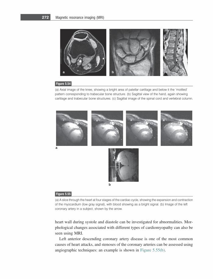
heart wall during systole and diastole can be investigated for abnormalities. Mor-phological changes associated with different types of cardiomyopathy can also beseen using MRI.
Left anterior descending coronary artery disease is one of the most commoncauses of heart attacks, and stenoses of the coronary arteries can be assessed usingangiographic techniques: an example is shown in Figure 5.55(b).
a b c
Figure 5.54
(a) Axial image of the knee, showing a bright area of patellar cartilage and below it the ‘mottled’pattern corresponding to trabecular bone structure. (b) Sagittal view of the hand, again showingcartilage and trabecular bone structures. (c) Sagittal image of the spinal cord and vertebral column.
a
b
Figure 5.55
(a) A slice through the heart at four stages of the cardiac cycle, showing the expansion and contractionof the myocardium (low gray signal), with blood showing as a bright signal. (b) Image of the leftcoronary artery in a subject, shown by the arrow.
272 Magnetic resonance imaging (MRI)
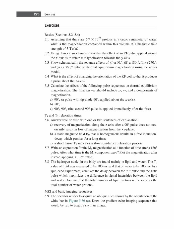
Exercises
Basics (Sections 5.2–5.4)5.1 Assuming that there are 6.7 3 1022 protons in a cubic centimeter of water,
what is the magnetization contained within this volume at a magnetic fieldstrength of 3 Tesla?
5.2 Using classical mechanics, show that the effect of an RF pulse applied aroundthe x-axis is to rotate z-magnetization towards the y-axis.
5.3 Show schematically the separate effects of: (i) a 90x�, (ii) a 180x�, (iii) a 270x�,and (iv) a 360x� pulse on thermal equilibrium magnetization using the vectormodel.
5.4 What is the effect of changing the orientation of the RF coil so that it producesa pulse about the z-axis?
5.5 Calculate the effects of the following pulse sequences on thermal equilibriummagnetization. The final answer should include x-, y-, and z-components ofmagnetization.a) 90�x (a pulse with tip angle 90�, applied about the x-axis).b) 80�x.c) 90�x 90�y (the second 90� pulse is applied immediately after the first).
T1 and T2 relaxation times5.6 Answer true or false with one or two sentences of explanation:
a) recovery of magnetization along the z-axis after a 90� pulse does not nec-essarily result in loss of magnetization from the xy-plane;
b) a static magnetic field B0 that is homogeneous results in a free inductiondecay which persists for a long time;
c) a short tissue T1 indicates a slow spin-lattice relaxation process.5.7 Write an expression for the Mz magnetization as a function of time after a 180�
pulse. After what time is the Mz component zero? Plot the magnetization afterinstead applying a 135� pulse.
5.8 The hydrogen nuclei in the body are found mainly in lipid and water. The T2
value of lipid was measured to be 100 ms, and that of water to be 500 ms. In aspin-echo experiment, calculate the delay between the 90� pulse and the 180�pulse which maximizes the difference in signal intensities between the lipidand water. Assume that the total number of lipid protons is the same as thetotal number of water protons.
MRI and basic imaging sequences5.9 The operator wishes to acquire an oblique slice shown by the orientation of the
white bar in Figure 5.56 (a). Draw the gradient echo imaging sequence thatwould be run to acquire such an image.
273 Exercises
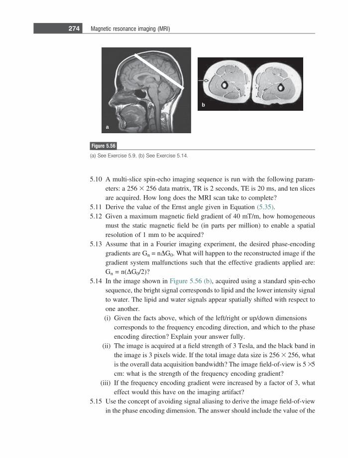
5.10 A multi-slice spin-echo imaging sequence is run with the following param-eters: a 256 3 256 data matrix, TR is 2 seconds, TE is 20 ms, and ten slicesare acquired. How long does the MRI scan take to complete?
5.11 Derive the value of the Ernst angle given in Equation (5.35).5.12 Given a maximum magnetic field gradient of 40 mT/m, how homogeneous
must the static magnetic field be (in parts per million) to enable a spatialresolution of 1 mm to be acquired?
5.13 Assume that in a Fourier imaging experiment, the desired phase-encodinggradients are Gn = nDG0. What will happen to the reconstructed image if thegradient system malfunctions such that the effective gradients applied are:Gn = n(DG0/2)?
5.14 In the image shown in Figure 5.56 (b), acquired using a standard spin-echosequence, the bright signal corresponds to lipid and the lower intensity signalto water. The lipid and water signals appear spatially shifted with respect toone another.(i) Given the facts above, which of the left/right or up/down dimensions
corresponds to the frequency encoding direction, and which to the phaseencoding direction? Explain your answer fully.
(ii) The image is acquired at a field strength of 3 Tesla, and the black band inthe image is 3 pixels wide. If the total image data size is 256 3 256, whatis the overall data acquisition bandwidth? The image field-of-view is 5 35cm: what is the strength of the frequency encoding gradient?
(iii) If the frequency encoding gradient were increased by a factor of 3, whateffect would this have on the imaging artifact?
5.15 Use the concept of avoiding signal aliasing to derive the image field-of-viewin the phase encoding dimension. The answer should include the value of the
a
b
Figure 5.56
(a) See Exercise 5.9, (b) See Exercise 5.14.
274 Magnetic resonance imaging (MRI)
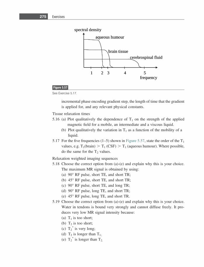
incremental phase encoding gradient step, the length of time that the gradientis applied for, and any relevant physical constants.
Tissue relaxation times5.16 (a) Plot qualitatively the dependence of T1 on the strength of the applied
magnetic field for a mobile, an intermediate and a viscous liquid.(b) Plot qualitatively the variation in T1 as a function of the mobility of a
liquid.5.17 For the five frequencies (1–5) shown in Figure 5.57, state the order of the T1
values, e.g. T1(brain) . T1 (CSF) . T1 (aqueous humour). Where possible,do the same for the T2 values.
Relaxation weighted imaging sequences5.18 Choose the correct option from (a)-(e) and explain why this is your choice.
The maximum MR signal is obtained by using:(a) 90� RF pulse, short TE, and short TR;(b) 45� RF pulse, short TE, and short TR;(c) 90� RF pulse, short TE, and long TR;(d) 90� RF pulse, long TE, and short TR;(e) 45� RF pulse, long TE, and short TR.
5.19 Choose the correct option from (a)-(e) and explain why this is your choice.Water in tendons is bound very strongly and cannot diffuse freely. It pro-duces very low MR signal intensity because:(a) T1 is too short;(b) T2 is too short;(c) T2
* is very long;(d) T2 is longer than T1;
(e) T2* is longer than T2.
spectral density
frequency
aqueous humour
brain tissuecerebrospinal fluid
1 2 3 4 5
spectral density
frequency
aqueous humour
brain tissuecerebrospinal fluid
1 2 3 4 5
Figure 5.57
See Exercise 5.17.
275 Exercises
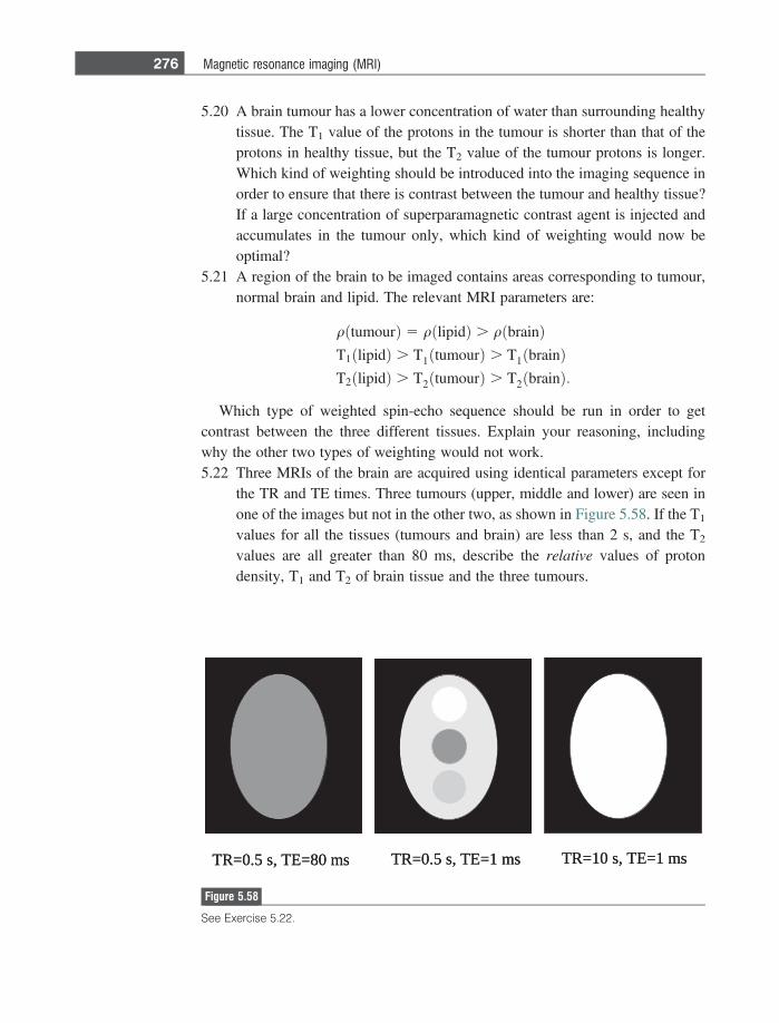
5.20 A brain tumour has a lower concentration of water than surrounding healthytissue. The T1 value of the protons in the tumour is shorter than that of theprotons in healthy tissue, but the T2 value of the tumour protons is longer.Which kind of weighting should be introduced into the imaging sequence inorder to ensure that there is contrast between the tumour and healthy tissue?If a large concentration of superparamagnetic contrast agent is injected andaccumulates in the tumour only, which kind of weighting would now beoptimal?
5.21 A region of the brain to be imaged contains areas corresponding to tumour,normal brain and lipid. The relevant MRI parameters are:
qðtumourÞ 5 qðlipidÞ . qðbrainÞT1ðlipidÞ . T1ðtumourÞ . T1ðbrainÞT2ðlipidÞ . T2ðtumourÞ . T2ðbrainÞ:
Which type of weighted spin-echo sequence should be run in order to getcontrast between the three different tissues. Explain your reasoning, includingwhy the other two types of weighting would not work.5.22 Three MRIs of the brain are acquired using identical parameters except for
the TR and TE times. Three tumours (upper, middle and lower) are seen inone of the images but not in the other two, as shown in Figure 5.58. If the T1
values for all the tissues (tumours and brain) are less than 2 s, and the T2
values are all greater than 80 ms, describe the relative values of protondensity, T1 and T2 of brain tissue and the three tumours.
sm 1=ET ,s 01=RTsm 1=ET ,s 5.0=RTsm 08=ET ,s 5.0=RT sm 1=ET ,s 01=RTsm 1=ET ,s 5.0=RTsm 08=ET ,s 5.0=RT
Figure 5.58
See Exercise 5.22.
276 Magnetic resonance imaging (MRI)
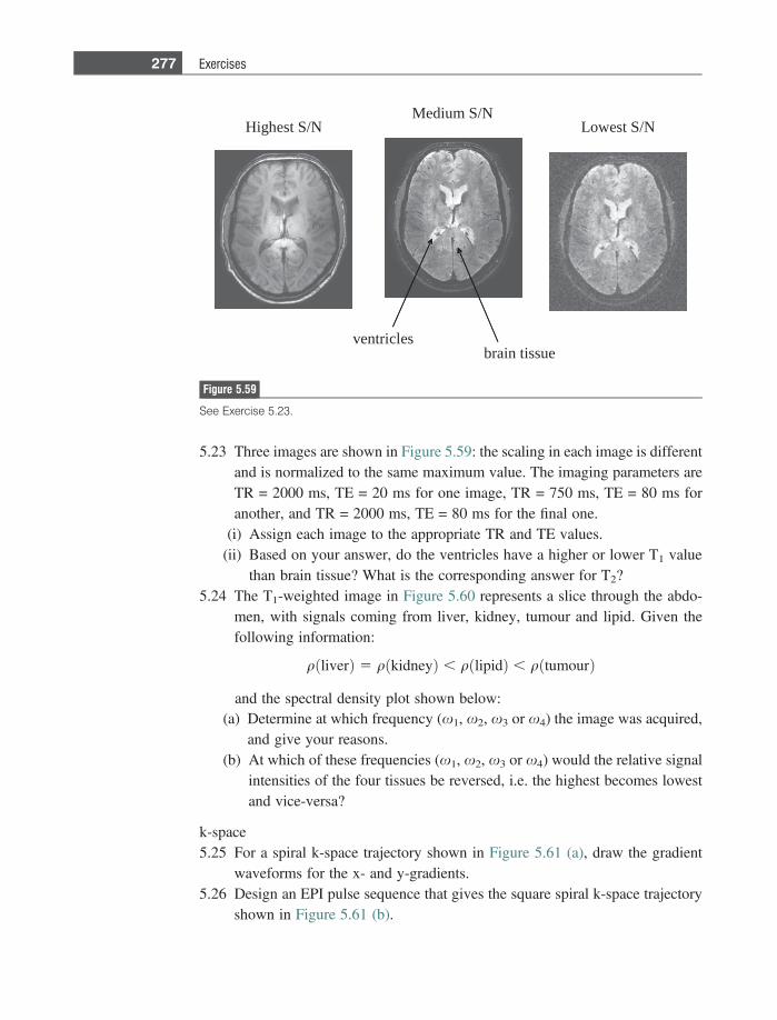
5.23 Three images are shown in Figure 5.59: the scaling in each image is differentand is normalized to the same maximum value. The imaging parameters areTR = 2000 ms, TE = 20 ms for one image, TR = 750 ms, TE = 80 ms foranother, and TR = 2000 ms, TE = 80 ms for the final one.
(i) Assign each image to the appropriate TR and TE values.(ii) Based on your answer, do the ventricles have a higher or lower T1 value
than brain tissue? What is the corresponding answer for T2?5.24 The T1-weighted image in Figure 5.60 represents a slice through the abdo-
men, with signals coming from liver, kidney, tumour and lipid. Given thefollowing information:
qðliverÞ 5 qðkidneyÞ , qðlipidÞ , qðtumourÞ
and the spectral density plot shown below:(a) Determine at which frequency (x1, x2, x3 or x4) the image was acquired,
and give your reasons.(b) At which of these frequencies (x1, x2, x3 or x4) would the relative signal
intensities of the four tissues be reversed, i.e. the highest becomes lowestand vice-versa?
k-space5.25 For a spiral k-space trajectory shown in Figure 5.61 (a), draw the gradient
waveforms for the x- and y-gradients.5.26 Design an EPI pulse sequence that gives the square spiral k-space trajectory
shown in Figure 5.61 (b).
Highest S/NMedium S/N
Lowest S/N
ventriclesbrain tissue
Figure 5.59
See Exercise 5.23.
277 Exercises
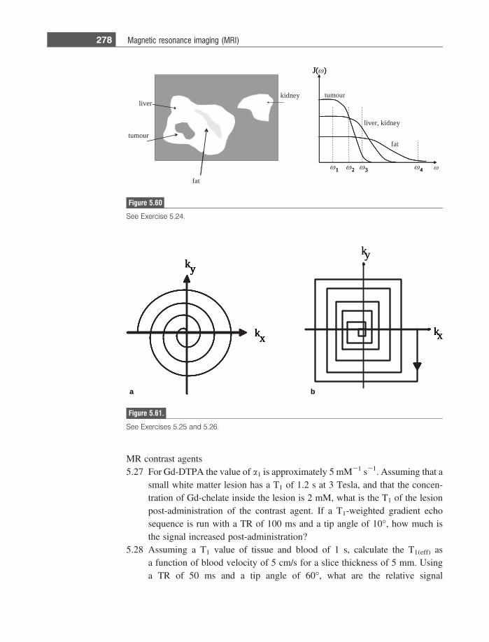
MR contrast agents5.27 For Gd-DTPA the value of a1 is approximately 5 mM21 s21. Assuming that a
small white matter lesion has a T1 of 1.2 s at 3 Tesla, and that the concen-tration of Gd-chelate inside the lesion is 2 mM, what is the T1 of the lesionpost-administration of the contrast agent. If a T1-weighted gradient echosequence is run with a TR of 100 ms and a tip angle of 10�, how much isthe signal increased post-administration?
5.28 Assuming a T1 value of tissue and blood of 1 s, calculate the T1(eff) asa function of blood velocity of 5 cm/s for a slice thickness of 5 mm. Usinga TR of 50 ms and a tip angle of 60�, what are the relative signal
kx
ky
kx
ky
kx
ky
kxkx
kyky
kx
ky
a b
Figure 5.61.
See Exercises 5.25 and 5.26.
revilyendik
ruomut
taf
tumour
liver, kidney
fat
1
J( )
2 3 4 ω ω 1
J(ω )
ω 2 ω 3 ω 41
J( )
2 3 4
Figure 5.60
See Exercise 5.24.
278 Magnetic resonance imaging (MRI)
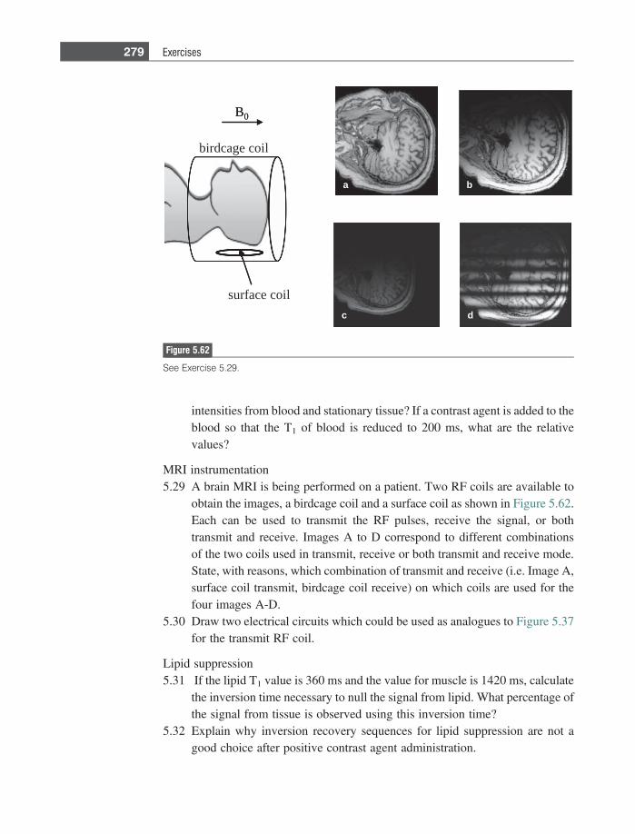
intensities from blood and stationary tissue? If a contrast agent is added to theblood so that the T1 of blood is reduced to 200 ms, what are the relativevalues?
MRI instrumentation5.29 A brain MRI is being performed on a patient. Two RF coils are available to
obtain the images, a birdcage coil and a surface coil as shown in Figure 5.62.Each can be used to transmit the RF pulses, receive the signal, or bothtransmit and receive. Images A to D correspond to different combinationsof the two coils used in transmit, receive or both transmit and receive mode.State, with reasons, which combination of transmit and receive (i.e. Image A,surface coil transmit, birdcage coil receive) on which coils are used for thefour images A-D.
5.30 Draw two electrical circuits which could be used as analogues to Figure 5.37for the transmit RF coil.
Lipid suppression5.31 If the lipid T1 value is 360 ms and the value for muscle is 1420 ms, calculate
the inversion time necessary to null the signal from lipid. What percentage ofthe signal from tissue is observed using this inversion time?
5.32 Explain why inversion recovery sequences for lipid suppression are not agood choice after positive contrast agent administration.
birdcage coil
surface coil
B0B0
a b
c d
Figure 5.62
See Exercise 5.29.
279 Exercises
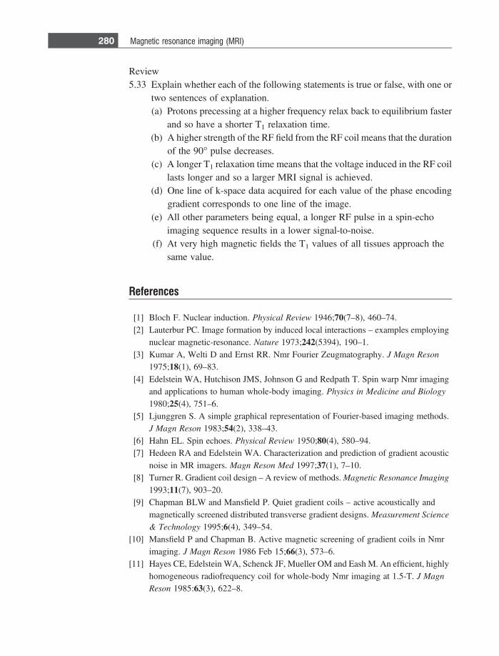
Review5.33 Explain whether each of the following statements is true or false, with one or
two sentences of explanation.(a) Protons precessing at a higher frequency relax back to equilibrium faster
and so have a shorter T1 relaxation time.(b) A higher strength of the RF field from the RF coil means that the duration
of the 90� pulse decreases.(c) A longer T1 relaxation time means that the voltage induced in the RF coil
lasts longer and so a larger MRI signal is achieved.(d) One line of k-space data acquired for each value of the phase encoding
gradient corresponds to one line of the image.(e) All other parameters being equal, a longer RF pulse in a spin-echo
imaging sequence results in a lower signal-to-noise.(f) At very high magnetic fields the T1 values of all tissues approach the
same value.
References
[1] Bloch F. Nuclear induction. Physical Review 1946;70(7–8), 460–74.[2] Lauterbur PC. Image formation by induced local interactions – examples employing
nuclear magnetic-resonance. Nature 1973;242(5394), 190–1.[3] Kumar A, Welti D and Ernst RR. Nmr Fourier Zeugmatography. J Magn Reson
1975;18(1), 69–83.[4] Edelstein WA, Hutchison JMS, Johnson G and Redpath T. Spin warp Nmr imaging
and applications to human whole-body imaging. Physics in Medicine and Biology
1980;25(4), 751–6.[5] Ljunggren S. A simple graphical representation of Fourier-based imaging methods.
J Magn Reson 1983;54(2), 338–43.[6] Hahn EL. Spin echoes. Physical Review 1950;80(4), 580–94.[7] Hedeen RA and Edelstein WA. Characterization and prediction of gradient acoustic
noise in MR imagers. Magn Reson Med 1997;37(1), 7–10.[8] Turner R. Gradient coil design – A review of methods. Magnetic Resonance Imaging
1993;11(7), 903–20.[9] Chapman BLW and Mansfield P. Quiet gradient coils – active acoustically and
magnetically screened distributed transverse gradient designs. Measurement Science
& Technology 1995;6(4), 349–54.[10] Mansfield P and Chapman B. Active magnetic screening of gradient coils in Nmr
imaging. J Magn Reson 1986 Feb 15;66(3), 573–6.[11] Hayes CE, Edelstein WA, Schenck JF, Mueller OM and Eash M. An efficient, highly
homogeneous radiofrequency coil for whole-body Nmr imaging at 1.5-T. J Magn
Reson 1985:63(3), 622–8.
280 Magnetic resonance imaging (MRI)
[12] Roemer PB, Edelstein WA, Hayes CE, Souza SP and Mueller OM. The NMR phasedarray. Magn Reson Med 1990 Nov;16(2), 192–225.
[13] Edelstein WA, Hardy CJ and Mueller OM. Electronic decoupling of surface-coilreceivers for Nmr imaging and spectroscopy. J Magn Reson 1986 Mar;67(1),156–61.
[14] Carlson JW and Minemura T. Imaging time reduction through multiple receiver coildata acquisition and image reconstruction. Magn Reson Med 1993;29(5), 681–7.
[15] Sodickson DK and Manning WJ. Simultaneous acquisition of spatial harmonics(SMASH): fast imaging with radiofrequency coil arrays. Magn Reson Med 1997Oct;38(4), 591–603.
[16] Pruessmann KP, Weiger M, Scheidegger MB and Boesiger P. SENSE: sensitivityencoding for fast MRI. Magn Reson Med 1999 Nov;42(5), 952–62.
[17] Griswold MA, Jakob PM, Heidemann RM et al. Generalized autocalibratingpartially parallel acquisitions (GRAPPA). Magn Reson Med 2002;47(6), 1202–10.
[18] Mansfield P. Multi-planar image-formation using Nmr spin echoes. Journal of
Physics C-Solid State Physics 1977;10(3), L55–L58.[19] Hennig J, Nauerth A and Friedburg H. RARE imaging: a fast imaging method for
clinical MR. Magn Reson Med 1986 Dec;3(6), 823–33.[20] Crooks LE, Mills CM, Davis PL, et al. Visualization of cerebral and vascular
abnormalities by NMR imaging. The effects of imaging parameters on contrast.Radiology 1982 Sep;144(4), 843–52.
[21] Ogawa S, Lee TM, Kay AR and Tank DW. Brain magnetic resonance imaging withcontrast dependent on blood oxygenation. Proc Natl Acad Sci U S A 1990Dec;87(24), 9868–72.
281 References

Index
absorbed dose, X-ray, 78, 79absorption, ultrasound, 153, 155
classical absorption, 155relaxation absorption, 154–5
accelerating voltage, 36, 40, 41, 55, 58, 63, 66,76, 83–4
accidental coincidences, 122, 131, 132, 133acoustic enhancement, 197acoustic shadowing, 20, 197, 202acoustic window, 167active shielding, gradient coils, 246aliasing
MRI, 252, 274pulsed wave Doppler, 184
A-mode scans, ultrasound, 175, 176, 199analogue-to-digital converter (ADC), 15, 17, 19, 47,
105Anger position network, 102, 103, 104, 106, 109,
126, 141, 144angular momentum, proton, 206–7, 210annihilation coincidence detection, 127, 128annular array, ultrasound, 174See also phased arrays, ultrasoundanti-scatter grid, 34, 35, 48, 49, 50–1, 53, 56, 59, 63,
68, 85, 90, 93, 97, 141attenuation coefficient, nuclear medicine, 25, 102,
103, 114, 115, 119, 126, 140attenuation coefficient, ultrasound, 46, 155, 156,
199, 202attenuation coefficient, X-ray, 25, 45, 46, 52, 53, 66,
71, 75, 81, 83, 84, 86, 101attenuation correction, nuclear medicine, 114, 116,
122, 130–1, 142axial resolution, ultrasound, 159, 163, 179, 184
backprojection, 24–5, 26, 27, 29, 33filtered backprojection, 2, 21, 24–5, 27, 28, 29,
66, 71, 72, 73, 75, 77, 86, 88, 110, 114, 115,123
beam forming, ultrasound, 173, 177beam hardening, X-ray, 74, 75, 83, 86beam steering, ultrasound, 169bevel angle, X-ray source, 38, 39, 48, 62, 85birdcage coil, MRI, 248, 249, 279bismuth germanate PET detectors, 122, 125, 126,
128, 133, 136Bloch equations, 215
block detector design, PET, 126blood brain barrier (BBB), 81, 262, 269blood oxygen level dependent (BOLD)
effect, 259B-mode scans, ultrasound, 169, 175, 176, 177, 179,
180, 184, 185, 187, 191, 194, 195, 196, 199,200, 201
Boltzmann equation, 207bow-tie filter, CT, 75bremsstrahlung radiation, X-ray, 41Bucky factor, 49
cadmium zinc telluride (CZT) detectors, PET, 119,120
caesium iodide (CsI), 52, 53, 54, 54–5, 57, 64cardiac catheterization, 64cardiac stress test, 89, 117, 118cavitation, ultrasound, 192Chang’s multiplicative method, attenuation
correction, 114characteristic acoustic impedance, 146–7, 148–9,
151, 158, 199characteristic radiation, X-ray, 41, 42charge coupled device (CCD), 5, 6, 64chemical shift, 220, 267clinical applications
CT, 80–1MRI, 268–9, 271–3, 275, 277, 279PET/CT, 137, 139, 141, 143planar scintigraphy, 109–111planar X-ray, 64–5SPECT, SPECT/CT, 117, 119, 121ultrasound, 193, 195–6
clutter, ultrasound, 178, 179, 191coincidence resolving time, 125, 127, 128, 132collimators
CT, 66, 68nuclear medicine, 90, 93, 97, 99, 100, 108, 109,
140, 141PET, 129SPECT, 111, 113, 120X-ray, 47
compound scanning, ultrasound, 177compressibility of tissue, 147, 149, 151Compton scatter
nuclear medicine, 90, 93, 101, 105, 109, 113,140, 142
PET, 134, 135X-ray, 42, 43, 45, 46, 47, 48, 50–1, 53, 56, 58,
63, 85computed radiography, 49, 50, 51, 85, 88computed tomography dose index (CTDI), 79contrast agents
MRI, paramagnetic, Gd-based, 69, 84, 85, 114,125, 261, 262
MRI, superparamagnetic, iron oxides, 261, 263,276
ultrasound, microbubbles, 146, 187, 188, 189,190, 191
X-ray, barium-based, 59, 60, 65, 72X-ray, iodine-based, 61
contrast-to-noise ratio (CNR), 1, 4, 12MRI, 237, 238, 261, 266nuclear medicine, 98, 108, 141, 142PET, 134ultrasound, 179X-ray, 2, 42, 48, 56, 58, 62
convolution, 8, 9, 14, 23, 24, 27, 28, 31, 57CT number, 71, 72, 75, 80cyclotron, 89, 123–125, 127
damping, transducer, 159, 160, 161, 163, 179, 245dead time of detector, 106–108, 134depth-of-focus (DOF), ultrasound, 165detector quantum efficiency (DQE), 56deterministic radiation effects, 77, 78diffusion-weighted MRI, 269digital radiography, 3, 50, 52, 64, 88digital subtraction angiography (DSA), 61, 62, 76Doppler ultrasound, 146, 152, 177, 179, 180, 181,
182, 183, 184, 185, 187, 189, 191, 192, 193,194, 196, 201, 202, 203
colour flow imaging, 194continuous wave Doppler, 186–187, 189power Doppler, 186pulsed wave Doppler, 181, 186spectral display, 182
dual energy CT, 75, 115dual energy window, nuclear medicine, 113, 133dual source CT, 75duplex ultrasound, 182dynamic focusing, ultrasound, 169, 170, 171, 174,
199dynamic range, receiver, 16, 52, 156, 172, 198dynode, photomultiplier tube, 101
echo planar MRI, 255echocardiography, 175, 187, 196, 203eddy currents, 246edge detection, 14effective atomic number, 43, 46, 125effective dose, radiation, 78, 79electron capture, 93energy resolution, nuclear medicine, 105, 106, 113,
119, 127, 133, 136energy spectrum, X-ray, 40, 40–43, 58, 105Ernst angle, 233, 259, 274, 280exposure time, X-rays, 39, 55
fan-beam reconstruction, CT, 73Faraday’s law of induction, MRI, 213, 220, 241,
247, 264figure-of-merit, gradient coils, 246fingerprint gradient coils, 246, 247flat panel detector, X-ray, 34, 76, 85fluorodeoxyglucose (FDG), 124, 134, 137, 139,
141, 143fluoroscopy, X-ray, 34, 63, 64, 88f-number, transducer, 163focal distance, ultrasound, 164focal plane, ultrasound, 165focal spot, X-ray, 38, 39, 57, 62, 66, 71, 76, 85, 88,
178, 191focused transducer, 163, 199Fourier pairs, 21Fourier transform, 2, 9, 20–21, 22, 23–24, 28, 32,
183, 220, 225, 230, 231, 239frame rate, ultrasound, 145, 169, 176, 200Fraunhofer zone, 161free induction decay (FID), 220frequency compounding, ultrasound, 177frequency encoding, MRI, 223, 228, 229, 232, 236,
239, 274Fresnel zone, 161full-width-half-maximum (FWHM), 6, 7, 31, 105,
106, 135, 141, 162functional MRI (fMRI), 259
gamma camera, 90, 97, 98, 99, 101, 103, 105–107,112, 126, 140
gamma rays, 140 keV monoenergetic, 89, 92–93geometric unsharpness, X-ray, 24, 57, 58, 63, 85gradient coils, MRI, 204, 205, 221, 241gradient echo sequences, MRI, 232, 233, 236, 239,
264, 273, 278grating lobes, transducer, 178grid frequency, 49grid ratio, 49, 53, 56, 63, 85gyromagnetic ratio, 207
half value layer (HVL), 47half-life, 91, 91–92, 114, 140, 143, 263harmonic imaging, ultrasound, 146, 177, 190, 191,
193, 194, 196, 203heel effect, 38, 39helical CT, 35, 36, 67–69, 70, 71, 73, 74, 75high-pass filter, 12, 29Hounsfield units, 25, 71
image artifacts, 10, 17, 20, 27CT, 20MRI, 20, 246, 253, 255, 269, 271nuclear medicine, 102ultrasound, 162, 177, 186, 194, 197
impedance matching, RF coils, 247inner sphere relaxation, 261, 262intravenous pyelogram (IVP), 65inverse Radon transform, 71inversion recovery sequences, MRI, 268, 279iterative reconstructions, 77, 110, 115, 123, 131, 133
284 Index
K-edge, 46, 53, 59kidney-urinary-bladder (KUB) scan, 65k-space, 21, 22, 229, 230, 231, 252, 253, 254, 255,
256, 277, 280
Larmor frequency, 210, 212, 214, 236, 239, 247,248
lateral resolution, ultrasound, 163, 164, 165, 169,178, 190, 194, 199, 200
lead zirconate titanate (PZT), 157, 158, 159, 161,164, 199
light spread function, 51, 52, 101, 126line spread function (LSF), 5, 6, 7, 8, 24, 25, 58linear arrays, ultrasound, 166–7line-of-reconstruction (LOR), 122, 123, 127, 131,
132, 135, 136lipid suppression techniques, MRI, 267–8lipid, MRI signal, 23, 46, 204, 205, 219, 267, 268,
270, 273, 274, 276, 279lipid, X-ray signal, 46, 47logic pulse, PET, 127, 128low-pass filter, 13lutetium orthosilicate (LSO), 125, 126, 127,
136
magnet, MRI, 204, 205, 206, 207, 214, 218, 221,235, 241, 242, 243, 244, 245, 246, 247, 249,250, 274
magnetic field gradient, MRI, 204, 241, 245, 274magnetic moment, 206, 209, 212, 219magnetic resonance angiography (MRA), 257magnetic susceptibility, tissue, 218, 260mammography, 34, 37, 38, 39, 42, 47, 50, 51, 62,
63, 268matching layer, ultrasound, 159, 198, 199maximum intensity projection (MIP), 259maximum-likelihood expectation-maximum
(ML-EM) method, 116mechanical index (MI), 190, 192metastable state, technetium, 93M-mode scans, ultrasound, 175, 176, 192, 196modulation transfer function (MTF), 5, 8, 9, 15, 24,
25, 31, 32, 57, 85multiple channel analyzer (MCA), 105multiple coincidences, PET, 131, 133, 134multiple-energy window, 113multiplicative reduction factor, TOF PET, 136multislice CT, 70, 71, 116myocardial perfusion, 89, 97, 110, 117, 118, 119,
196
near-field boundary (NFB), ultrasound, 161non-linear effects, ultrasound, 188, 189Nyquist frequency, 18, 19, 33
opthalmic pachymetry, 175outer sphere relaxation, 262oversampling, 19, 251
parallel imaging, MRI, 252–3, 254partial volume effect, 12, 109, 116, 261, 266
penumbra, X-ray, 57, 58PET/CT, principles, 130–131phase encoding, MRI, 223, 226, 227, 230, 231, 232,
237, 239, 252, 255, 265, 274, 280phased arrays, MRI, 249, 252–255phased arrays, ultrasound, 167, 171–2
annular array, 174multi-dimensional array, 173–4
photocathode, 101photoelectric interactions, 42–3, 44, 46, 47, 58, 59,
101photoelectron, 102photomultiplier tubes, 90, 100, 125photopeak, 105, 106, 113, 133piezoelectric materials, 157, 160, 161, 163, 165,
166, 174point spread function (PSF), 5, 7, 8, 9, 9–11, 12, 30,
85, 134, 141Poisson distribution, 54, 55, 56, 85, 108positron annihilation, 123precession, 209, 211, 212, 214, 218, 221, 222, 224,
264proton density, MRI, 229, 233, 234, 236, 261, 266,
276pulse height analyzer (PHA), 105, 106, 127pulse inversion, ultrasound, 146, 190pulse repetition rate (PRR), 160, 181, 184pulsed mode Doppler, 181
quadrature detector, 172, 182, 187quality (Q) factor, ultrasound transducer, 161
radiation dose, 11, 36, 55, 57, 62, 68, 77, 79, 80, 92,196
radiation weighting factor, 78radioactive dose, 92, 93, 118, 140radioactivity, 6, 33, 90, 92, 95–6, 102, 139, 140,
142, 143radiofrequency (RF) coils, MRI, 241, 247, 248, 250,
265, 273, 279, 280radiotracers, 89, 91, 93, 97, 99, 103, 106, 108, 109,
109–111, 112, 113, 114, 118, 121, 134, 137,139, 140
Ramachandran-Lakshminarayanan (Ram-Lak)filter, 29
Rayleigh scattering, ultrasound, 152, 153receiver operator characteristic (ROC) curve, 2, 4,
30reflection, ultrasound, 53, 152, 153, 155refraction, ultrasound, 125, 152, 197, 201relaxation absorption coefficient, ultrasound, 154reverberation artifact, ultrasound, 197robotic synthesis, PET, 124rotating reference frame, MRI, 214, 215, 217, 222,
227
safety levels, ultrasound, 191sampling rate, 8, 16, 18, 24, 31, 53, 251, 255scatter correction, 112, 113, 115, 133scintillation crystal, 90, 100, 101, 106, 109, 125,
140
285 Index
sensitivity, ROC analysis, 2, 4, 30Shepp-Logan phantom, 29shim coils, MRI, 244side lobes, ultrasound transducer, 162signal averaging, 10, 11signal-to-noise ratio (SNR), 1, 4, 10–12, 13, 29, 52,
57, 101, 136, 265, 266MRI, 2, 214, 233, 234, 237, 241, 266nuclear medicine, 90, 98, 108, 111, 140, 141PET, 121, 123, 129, 134ultrasound, 178, 179X-ray, 54, 55, 57, 58, 59
sinogram, 27, 28, 29, 33, 86, 88, 116, 142slice selection, MRI, 223slip ring, CT, 69sodium iodide crystal, thallium activated, 100–101,
102, 103, 104, 119sodium pertechnetate, 94, 96spatial frequency, 5, 9, 12, 20–3, 28, 29, 32, 231spatial resolution, 1, 2, 4, 5, 7, 9–11, 12–3, 58, 63,
99, 104, 178, 266, 274CT, 71MRI, 204, 231, 239, 252, 265, 265–6nuclear medicine, 90, 100, 108, 108–9, 140,
141PET, 125, 126, 127, 130, 134–5SPECT, 111ultrasound, 165, 178–9X-ray, 51, 57, 57–8, 63
spatial smoothing, 14, 131specific absorption rate (SAR), 267specificity, ROC analysis, 2, 4, 30speckle, 10, 152, 177, 178, 194, 197, 199SPECT/CT, 116–7spectral density, MRI, 240, 277speed of sound, 145, 146, 162, 199, 202spin–echo sequences, MRI, 235, 236, 237, 238, 254,
256, 257, 263, 273, 274, 276, 280spin–lattice relaxation time, T1, 216, 217, 228, 231,
236, 238, 257, 261, 262, 264, 266, 267, 268,273, 275, 276, 278, 279
spin-spin relaxation time, T2, 24, 216, 218, 231,234, 236, 238, 242, 255, 256, 257, 260, 261,264, 266, 267, 273, 275, 276
spiral CT, See helical CTstar artifact, backprojection, 26, 28stochastic radiation effects, 78subwindow, nuclear medicine, 113superconducting magnet, See magnet, MRIsurface coil, MRI, 279
technetium generator, 93, 94, 95–6, 140thermal index (TI), 152, 192, 193, 197, 198, 268thin-film transistor (TFT) arrays, 52time-gain compensation, ultrasound, 172time-of-flight (TOF) angiography, MRI, 257, 258,
259, 261, 270time-of-flight (TOF) PET, 123, 126, 135, 136, 143tip angle, MRI, 215, 233, 258, 265, 268, 273, 278tomosynthesis, X-ray, 76, 77transducer bandwidth, 159transducers, ultrasound, 145, 146
focused, 163, 165single element, 156, 161two-dimensional arrays, 165, 167, 169–71
transmit/receive switchesMRI, 250ultrasound, 156
tube current, X-ray, 39, 55, 66, 76, 84tube output, X-ray, 39turbo spin echo sequences, MRI, 256
vector model, MRI, 273
wave propagation, ultrasound, 146–7
X-ray tube, 10, 34, 36, 36–37, 39–41, 63, 70, 71,75, 85
z-flying spot technique, CT, 71z-signal, nuclear medicine, 105
286 Index