Embed Size (px)
Citation preview

통계연구(2014), 제19권 제1호, 107-137
The Impact of Expense Shocks on the Financial Distress of Korean Households
Jane Yoo1)
Abstract
The main objective of this study is to examine the major determinants of household
financial distress, particularly expense shocks that increase the probability of failure in loan
repayment. Using the survey of household finances published by Statistics Korea, the study
investigates expense shocks that result in a large proportion of household income being
allocated to debt repayment, thus limiting the funds available for consuming goods and/or
saving. I use a bootstrapped random effect probit model and two-stage least squares model.
In addition, in finding a variable’s optimal spit value and goodness of fit, I use an early
warning signal methodology. The test results present the following three categories of
expense shocks are sensitive to financial vulnerability: i) secured loans for debt repayment,
medical expenses, and daily expenses; ii) unsecured credits for debt repayment, medical
expenses and rents; iii) credit card loans for debt repayment, and rents.
Key words : Household financial stress, Unsecured credit, Logit model, Early warning signal
1. Introduction
Since the recent financial crisis, changes in household debt levels have become
an important indicator to inform us the current state of an economy. It also
contains the prominent implications on its future stability because total
consumption and investment is influenced by a household’s saving decision: when
a substantial proportion of household income is allocated to debt repayment,
households have fewer funds available to purchase goods or to start a business. A
high debt-to-income ratio increases the market’s vulnerability to unexpected
negative productivity shocks, as households are more likely to fail on their debt
obligations when they suffer unanticipated misfortune such as job losses or illness.
In addition, when household debt relative to income is high and unemployment is
rising, lenders may respond to the expected increase in the number of insolvent
accounts by limiting the availability of credit, which may further reduce total
spending. A household feels more vulnerable or less confident when her
1) Contact: [email protected]. An assistant professor in the department of Financial
Engineering, School of Business, Ajou University.
108 Jane Yoo
consumption expenditure soars under this stressful environment.
The household financial distress is also related to the structure and
sophistication of financial markets. For example, in the housing mortgage market,
the root of the recent US-led subprime crisis, lenders have developed products
that broaden the base of household debt by enabling borrowers to purchase homes
despite them having a low credit score or limited funds to make a down payment
on the home. Advances in home equity lending have also allowed borrowers to
extract equity-financing more easily from their homes, and this market has
expanded to the secondary market of cash-out refinancing at high interest rates.
In the same vein, car purchasers have a greater number of finance choices than
they did in the past, such as leasing or borrowing through installment loans.
Meanwhile, numbers of revolving accounts are also growing, according to the
annual report on credit card usage (G19 published by the Federal Reserve Bank,
New York) by both financial and non-financial businesses. As a result, it
underlies the connection between a household’s stress from using a specific loan
type according to expense shocks. This study contributes to the body of
knowledge on this topic by examining the situations that a household feels
vulnerable or is afraid of losing her creditworthiness due to the inability to repay
debts. By the recent technological development, we can encompass a wide range
of the origins of these shocks including medical expenses, wedding costs,
educational spending, and other investment plans.
Analyzing these expense shocks has been shown important by their strong
relation to household financial distress in much macroeconomic theoretical literature
(Athreya (2002), Li and Sartre (2006), and Athreya, et al. (2012)). Fay, Hurst and
White (2002) built a general equilibrium model with the unexpected expenditure
such as legal fees for divorce, or medical expenses for accidents or hospitalization.
The expenses raised the probability of insolvency, the degree of poverty, and the
rates of bankruptcy filings particularly when a household was lack of buffer stock
saving (Carroll (1997)). Some behavioral finance literature emphasized a
psychological factor when a household resolved the stress in an uncertain
environment. Clustering, herding, and flocking2) in a financial market are the
aggregate phenomena by the combination of a psychological factor and a lack in
credible information in a bad economy. To the best of my knowledge, this paper
is the first attempt to find a measurable financial health indicator that is strongly
related to a psychological factor in resulting the financial distress. The paper
provides details about the indicator including the goodness of fit in predicting the
severe stress, and the optimal split value in screening a vulnerable household.
2) See Banerjee (1992), and Shiller (2000) for more details in explaining the impact of a
psychological factor on a financial market.

The Impact of Expense Shocks on the Financial Distress of Korean Households 109
<Figure 1.1> Fitted Savings Plots on the Disposable Income3)
Figure 1.1 shows savings as a function of disposable income according to the
level of financial stress. The red dotted line represents savings of a representative
household who is under the financial distress. At the same level of disposable
income, a household, who is free from the stress, accumulates more savings than
those under the stress and the amount increases as her disposable income
increases (shown by black crosses). Given the lack of buffer stock for a
financially constrained household, Figure 1.2 shows the use of a disaggregated
loan corresponding to the level of income by the level of stress. Financially
constrained households, whose loans are drawn by the red dotted line, tend to
borrow more secured loans than a household without the constraint of the black
plots (in crosses). In the examination of the difference with other types of loans,
unsecured credit lines and credit card loans, the difference is negligible. Despite
the small size of the difference, credit card usage can be an efficient indicator at
margin to distinguish a household under the severe stress from those who are not.
This paper provides the detailed information about these determinants by focusing
on the goodness of fit rather than the simple marginal impact. An indicator’s
threshold can play a key role in minimizing the related costs when a policy maker
targets the reduction of the stress.
3) Source: The survey of household finance in 2010 and 2011. The Figure represents the
fitted line of household saving amounts on the disposable income after robust OLS
regression. Before regression, data are interpolated on 1000 grid points to minimize noise
with respect to clustered data around a low income quartile.
110 Jane Yoo
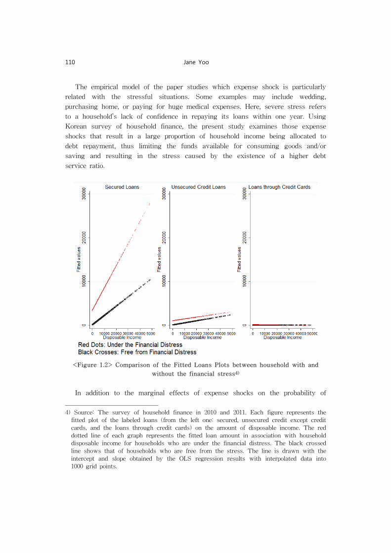
The empirical model of the paper studies which expense shock is particularly
related with the stressful situations. Some examples may include wedding,
purchasing home, or paying for huge medical expenses. Here, severe stress refers
to a household’s lack of confidence in repaying its loans within one year. Using
Korean survey of household finance, the present study examines those expense
shocks that result in a large proportion of household income being allocated to
debt repayment, thus limiting the funds available for consuming goods and/or
saving and resulting in the stress caused by the existence of a higher debt
service ratio.
<Figure 1.2> Comparison of the Fitted Loans Plots between household with and
without the financial stress4)
In addition to the marginal effects of expense shocks on the probability of
4) Source: The survey of household finance in 2010 and 2011. Each figure represents the
fitted plot of the labeled loans (from the left one: secured, unsecured credit except credit
cards, and the loans through credit cards) on the amount of disposable income. The red
dotted line of each graph represents the fitted loan amount in association with household
disposable income for households who are under the financial distress. The black crossed
line shows that of households who are free from the stress. The line is drawn with the
intercept and slope obtained by the OLS regression results with interpolated data into
1000 grid points.
The Impact of Expense Shocks on the Financial Distress of Korean Households 111
being under the stress, the empirical evidences presented in this study differ from
those of previous works in that it suggests an optimal split for each expense
category between safe and risky accounts for managing stress. The shortcomings
of the traditional binary response model include its limited analysis of the marginal
effect evaluated at the mean, under a restricted assumption on error terms, and its
inability to identify which indicators are more suitable for predictions. I resolve
these shortcomings by applying nonparametric estimations to our data. The results
of the EWS model suggest that the following three sudden expense shocks explain
a substantial degree of household vulnerability: i) secured loans for debt
repayment, medical expenses, and daily expenses; ii) unsecured credits for debt
repayment, medical expenses and rents; iii) credit card loans for debt repayment,
and rents. Based on these results, this study suggests that policy makers target
resolving these expense shocks, thus diminishing credit risks in the economy.
The empirical evidence presented herein emphasizes that using unsecured credit
accounts should be more closely analyzed when a lender or creditor attempts to
predict a borrower’s ability and willingness to repay debts. The study then
develops a screening tool that could be used before implementing a public policy
that targets the relief of certain types of debts.
The remainder of the paper comprises six sections. The next section briefly
discusses previous studies of household-level financial stresses and their
determinants. Section 3 describes the Korean data used in the study. Our
methodological models and strategies are presented in Section 4, and Section 5
discusses our results. Section 6 concludes the paper.
2. Literature review
There are far fewer empirical studies than theoretical works on the impact of
the type of loan in association with expense shocks on the household financial
stress. It is mainly because of limited access to the relevant microdata5) and a
lack of data on household-level credit management. Domowitz and Sartian (1999)
developed qualitative choice models by using sample cases compiled by the United
States General Account Office and a survey conducted by Consumer Finance
(related theoretical studies include Athreya (2002) and Li and Sartre (2006)). They
showed that medical and credit card debts were the strongest contributors to
bankruptcy. In the nested logit results in Fay et al. (2002), the financial benefit
5) In Korea, The Statistics Korea only began collecting micro data regularly in 2010,
following their first collection in 2006.

112 Jane Yoo
from the value of the debt of non-exempt assets affected the probability of filing
for bankruptcy. Credit card issuers and credit score reporting agencies also studied
this problem with their in-house data on customers’ credit history, income,
employment status, length of employment, and home-ownership. Similarly, Gross
and Souleles (2002) studied unsecured credit lines of delinquent debtors, and
Dawsey and Ausubel (2004) demonstrated a strategic delinquency choice. These
studies are closely related to drawing delinquency profiles based on consumption
and saving over a lifetime (see Attanasio and Browning (1995), Attanasio et al.
(1999), and Fernandez-Villaverde and Krueger (2011)). A few studies on
precautionary saving or the lifetime wealth, such as Carroll (1997) and Gourinchas
and Parker (2002), are also related with the literature.
Despite their findings on the marginal impact of explanatory variables, there
have been discussions on developing a more sophisticated methodology for better
estimation. Some economists in the International Monetary Fund and monetary
authorities concern on how to detect an efficient indicator, and how to determine
the criteria of the indicator in examining a household’s financial health. In order to
evaluate an explanatory power and to find the optimal split value, a traditional
regression models are not sufficient.
The level of household debt in Korean credit market has received attention
since the recent financial crisis. There are many studies that find the determinants
of insolvent accounts as well as ways in which to help those households. Kim and
Jeon (2000), for example, empirically examined the effectiveness of credit
measurements. By using the results provided by Lee and Jeong (2005) on the
current state of personal bankruptcy in Korea, they showed that the rate of credit
card usage, the most popular type of unsecured credit, and its sensitivity to
interest rate changes were the important factors in determining credit risk. It was
comparable with personal bankruptcy data from Japan and the US. Some empirical
studies, which use aggregate variables, support these micro-level findings by
emphasizing the role of commercial banks in buffering an adverse shock to the
market by releasing surplus funds before loanable funds dry up, which would
result in a worse constraint when the leverage is limited. In addition, most
dynamic analyses on the stress caused by household debt use dynamic general
equilibrium models with a Bayesian framework to evaluate the impulse response
function and variance decomposition given a shock (see Kim (2012), Kim and Kim
(2010)). Further, those models extended to cover empirical analyses most often
used logit or probit models, correcting for the heteroskedasticity (Kim et al.
(2009)). However, the work is limited because it used the aggregate level of debt
and probability of bankruptcy.

The Impact of Expense Shocks on the Financial Distress of Korean Households 113
3. Data
As the government became less confident about the distribution of loans to
households from the data provided by commercial banks in representing the
distribution of the credit market as a whole, it started to collect the data on
household budgets including assets, incomes, and debt levels. Statistics Korea, the
Bank of Korea, and the Financial Supervisory Service jointly conduct the Survey
of Household Finances to elaborate data on household-level credit risks. The
survey contains micro-level variables including demographic characteristics that
are not easily captured by aggregate variables. It also provides the information on
the household’s financial health: their financial distress and attitude to resolving
risks and stresses when managing a loan repayment schedule. Since the first
publication in 2006, the random sample was next drawn in 2010, and again in
2011. The attrition rate from 2010 to 2011 was approximately 10 percent.
In 2012, Statistics Korea expanded Survey of Household Finances by compiling
it with Living Condition data. It over-samples the population from the lowest
quintile to measure poverty factors in the country, thus helps developing a social
security program. This expansive sample includes detailed questions on
consumption expenditure and monthly interest payments as well as the selective
indicators of unemployment such as a job-seeking period. Given this structural
change in the survey, only the survey of household finance collections of 2010 and
2011 are used in our empirical tests.
Despite its advantage, only few studies have employed the micro-level works
using the survey. For example, Lee and Kim (2012) used the survey to measure
household credit risk, while Lee (2012) used the data in order to investigate
changes in the real estate prices from 2010 to 2011. He concluded that a high
proportion of the elderly were exposed to higher volatility risks in the housing
market. According to his analysis, the portfolio of the elderly, which is heavily
weighted by non-financial assets, is one of the major risks in the aggregate
economy, particularly when a market is experiencing real estate price risks.
Similarly, Park et al. (2012) used the survey to examine the features of lenders in
a financial sector and assessed their expected losses to measure the credit risks of
these lending institutions.
Income in this study refers to the conventional definition used by the Federal
Reserve Board since 1995. The survey of Korean household finance provides data
on household income, which may include wages/salaries, earnings from a
business/farm/sole proprietorship, non-tax investments, interest income, dividends,
gains or losses from the sale of stocks and bonds, net rent/royalties,
compensation, child support/alimony, and any other earnings. The category of
114 Jane Yoo
financial assets may include savings in transaction accounts (checking accounts, if
more than one), certificates of deposits, investments in saving bonds, bonds, stocks
(both public and equities associated with business ownership), pooled investment
funds, brokerage accounts, retirement accounts, other managed assets, and any
other saving plans. If a household has used a loan to purchase a financial asset,
the loan amount may be subtracted from the total asset value. Finally, the survey
also collects the market values of non-financial assets including vehicles, primary
residence, other properties, and equity in non-residential property at a cost-based
value.
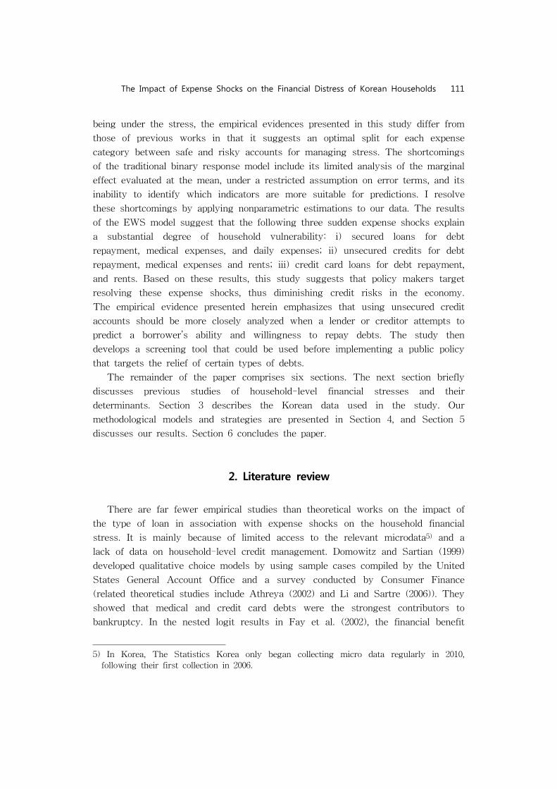
<Table 3.1> Summary statistics of demographic variables6)
Variable Mean Standard Deviation Min Median Max
Financial Stress 0.38 0.49 0 0 1
Age 51.32 14.67 17 50 95
Education 4.19 1.60 1 4 7
Number of Members in a Household
2.96 1.32 1 3 10
Marital Status(1 if married, 0 otherwise)
0.73 0.44 1 0 1
Number of Observations 19435
Total consumer debt comprises two major types: revolving and non-revolving
debt. Revolving credit plans include a prearranged limit and debt repayment plans
in one or more installments. This type of credit may be further classified into
unsecured and secured credit. The most popular types of unsecured, revolving
credit are credit card loans or cash advances through a card, which increase the
cumulative cost of borrowing as the length of repayment plan is extended. In
terms of secured credit, most households have revolving mortgage payment plans;
6) Source: The survey of household finance in 2010 and 2011. In the summary of statistics,
the unit of a variable refers to the structure of the survey. Because the survey collects
the data of a household balance sheet from a household head, a demographic variable
represents the characteristic of a head. Educational indicator is classified into seven
categories such as, 1: no education, 2: an elemetary level, 3: a junior high level, 4: high
school level, 5: college-educated, 6: an undergraduate level, 7: a post-graduate level.
There were four types with indicating a martial status, 1: single, 2: married, 3: divorced,
and 4: widowed. In this descriptive table, 1 if married, and 0 otherwise.
The Impact of Expense Shocks on the Financial Distress of Korean Households 115
however, unless there is any indication of deferring or extending the schedule, I
have classified this type of loan as non-revolving debt. The most common type of
non-revolving credit is closed-end credit, which is repaid on a prearranged
schedule. This credit can be secured or unsecured. Vehicle, education, and
consumer loans make up the majority of this type of credit, but other loans are
included as well such as personal loans and loans for debt repayment, business
management, and miscellaneous purposes. In this paper, the empirical analysis uses
only three types of loans, secured loans, unsecured credit loans except credit card
payments, and credit card loans. The total amount of loans is free from perfect
multicollinearity with the linear combination of these loans because the
miscellaneous loans, and borrowing for non-home-equity-financing are excluded in
a regression model. Table 3.1 and 3.2 summarize the descriptive statistics of
variables.
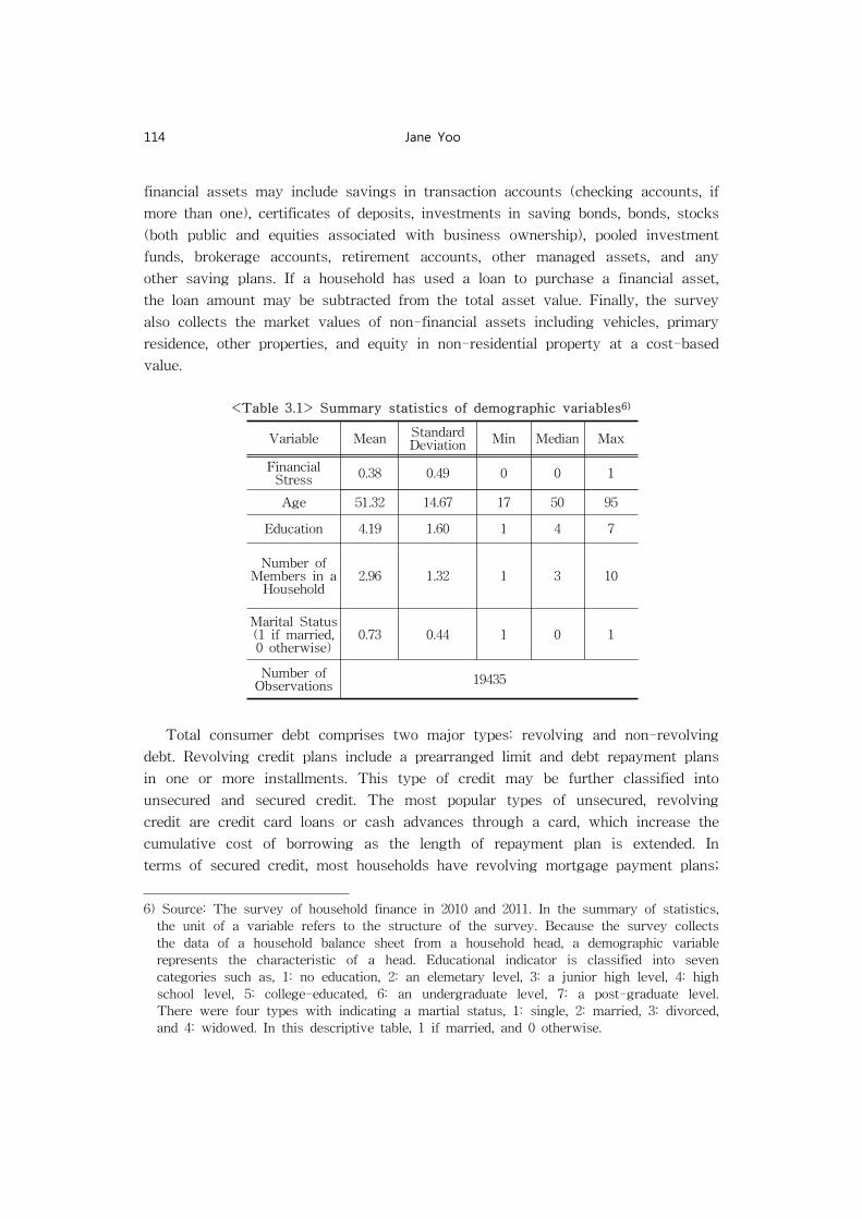
In addition, I define the financial distress of Korean households according to
responses to the question in the survey, “Do you think that you are willing
to/able to repay the outstanding amount of debt in a given schedule within the
next year?” If a household answers “yes,” I take this to indicate “no or minimal
stress.” On the contrary, if the answer is “no or unlikely,” then this is taken to
mean “high or significant stress.”
<Table 3.2> Summary statistics of variables in the Survey of Household Finance,
in ten thousands Won
Variable Mean Standard Deviation Median
Net worth 23,658 48111 12,399
Financial assets 6,372 11,714 3,056
Home equity value 11,541 19,505 4,500
The amount of saving 4,600 10,244 1,846
Disposable income 3,158 3,567 2,471
Expenditure 627 824 435
Debt 4,890 17,891 530
The total amount of loans 3,368 16,107 117
Secured loans 2,685 14,559 0
Unsecured credit loans (except credit card loans) 577 5,696 0
Credit card loans 45 359 0
The number of observations 19435
116 Jane Yoo
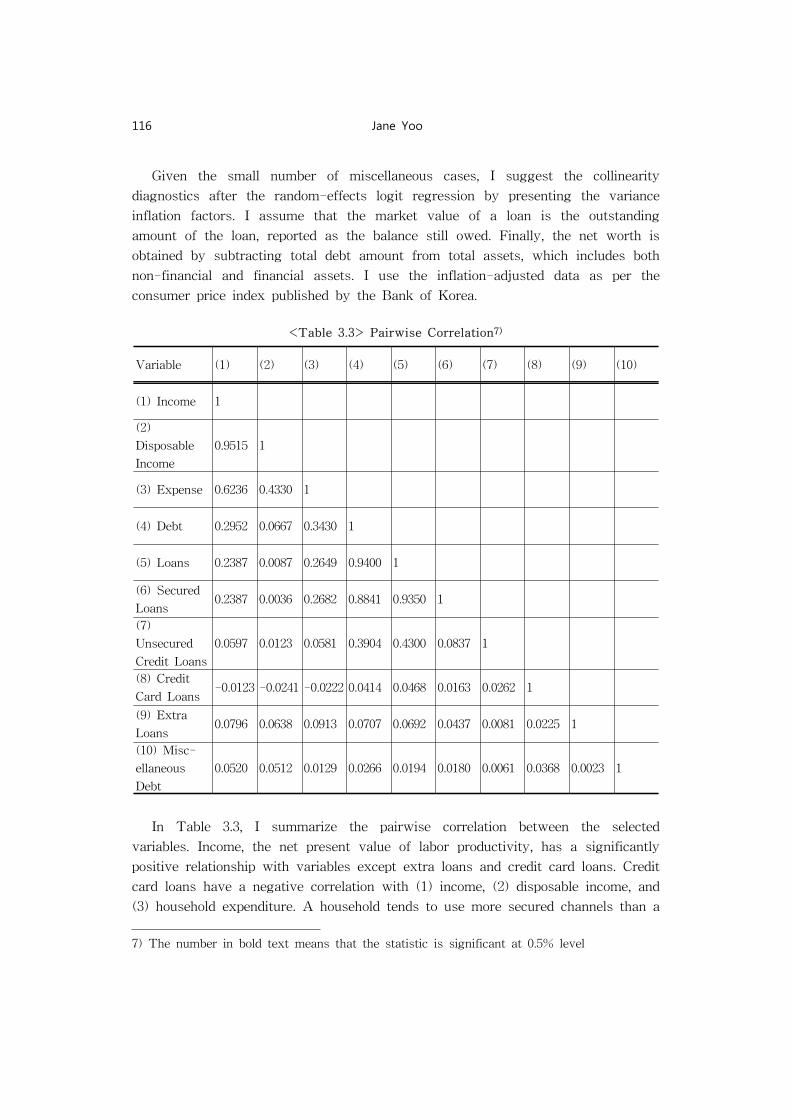
Given the small number of miscellaneous cases, I suggest the collinearity
diagnostics after the random-effects logit regression by presenting the variance
inflation factors. I assume that the market value of a loan is the outstanding
amount of the loan, reported as the balance still owed. Finally, the net worth is
obtained by subtracting total debt amount from total assets, which includes both
non-financial and financial assets. I use the inflation-adjusted data as per the
consumer price index published by the Bank of Korea.
<Table 3.3> Pairwise Correlation7)
Variable (1) (2) (3) (4) (5) (6) (7) (8) (9) (10)
(1) Income 1
(2)
Disposable
Income
0.9515 1
(3) Expense 0.6236 0.4330 1
(4) Debt 0.2952 0.0667 0.3430 1
(5) Loans 0.2387 0.0087 0.2649 0.9400 1
(6) Secured
Loans0.2387 0.0036 0.2682 0.8841 0.9350 1
(7)
Unsecured
Credit Loans
0.0597 0.0123 0.0581 0.3904 0.4300 0.0837 1
(8) Credit
Card Loans-0.0123 -0.0241 -0.0222 0.0414 0.0468 0.0163 0.0262 1
(9) Extra
Loans0.0796 0.0638 0.0913 0.0707 0.0692 0.0437 0.0081 0.0225 1
(10) Misc-
ellaneous
Debt
0.0520 0.0512 0.0129 0.0266 0.0194 0.0180 0.0061 0.0368 0.0023 1
In Table 3.3, I summarize the pairwise correlation between the selected
variables. Income, the net present value of labor productivity, has a significantly
positive relationship with variables except extra loans and credit card loans. Credit
card loans have a negative correlation with (1) income, (2) disposable income, and
(3) household expenditure. A household tends to use more secured channels than a
7) The number in bold text means that the statistic is significant at 0.5% level
The Impact of Expense Shocks on the Financial Distress of Korean Households 117
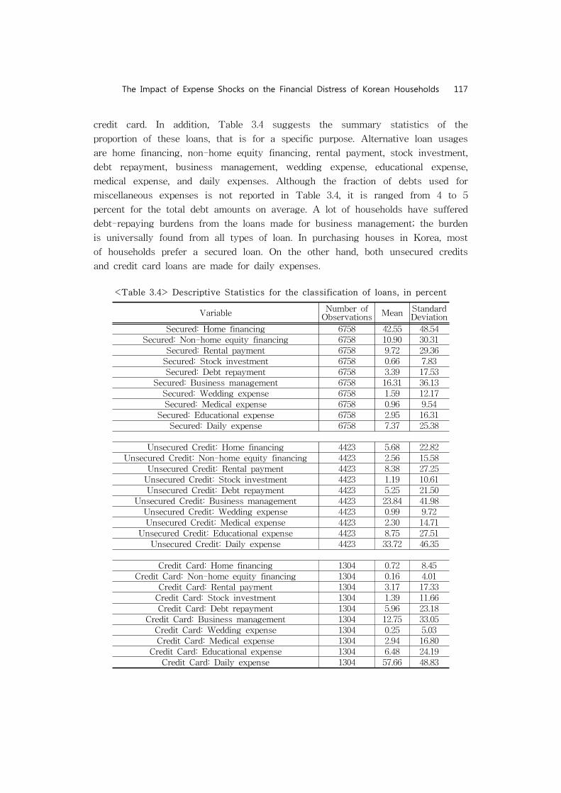
credit card. In addition, Table 3.4 suggests the summary statistics of the
proportion of these loans, that is for a specific purpose. Alternative loan usages
are home financing, non-home equity financing, rental payment, stock investment,
debt repayment, business management, wedding expense, educational expense,
medical expense, and daily expenses. Although the fraction of debts used for
miscellaneous expenses is not reported in Table 3.4, it is ranged from 4 to 5
percent for the total debt amounts on average. A lot of households have suffered
debt-repaying burdens from the loans made for business management; the burden
is universally found from all types of loan. In purchasing houses in Korea, most
of households prefer a secured loan. On the other hand, both unsecured credits
and credit card loans are made for daily expenses.
<Table 3.4> Descriptive Statistics for the classification of loans, in percent
Variable Number of Observations Mean Standard
Deviation
Secured: Home financing 6758 42.55 48.54
Secured: Non-home equity financing 6758 10.90 30.31
Secured: Rental payment 6758 9.72 29.36
Secured: Stock investment 6758 0.66 7.83
Secured: Debt repayment 6758 3.39 17.53
Secured: Business management 6758 16.31 36.13
Secured: Wedding expense 6758 1.59 12.17
Secured: Medical expense 6758 0.96 9.54
Secured: Educational expense 6758 2.95 16.31
Secured: Daily expense 6758 7.37 25.38
Unsecured Credit: Home financing 4423 5.68 22.82
Unsecured Credit: Non-home equity financing 4423 2.56 15.58
Unsecured Credit: Rental payment 4423 8.38 27.25
Unsecured Credit: Stock investment 4423 1.19 10.61
Unsecured Credit: Debt repayment 4423 5.25 21.50
Unsecured Credit: Business management 4423 23.84 41.98
Unsecured Credit: Wedding expense 4423 0.99 9.72
Unsecured Credit: Medical expense 4423 2.30 14.71
Unsecured Credit: Educational expense 4423 8.75 27.51
Unsecured Credit: Daily expense 4423 33.72 46.35
Credit Card: Home financing 1304 0.72 8.45
Credit Card: Non-home equity financing 1304 0.16 4.01
Credit Card: Rental payment 1304 3.17 17.33
Credit Card: Stock investment 1304 1.39 11.66
Credit Card: Debt repayment 1304 5.96 23.18
Credit Card: Business management 1304 12.75 33.05
Credit Card: Wedding expense 1304 0.25 5.03
Credit Card: Medical expense 1304 2.94 16.80
Credit Card: Educational expense 1304 6.48 24.19
Credit Card: Daily expense 1304 57.66 48.83

118 Jane Yoo
4. Estimation
This section describes two methodological strategies of the paper in estimating
the marginal impact of expense shocks on household vulnerability. First, I
introduce a traditional binary response model linked to a logistic or normal
distribution of errors. Although this model is widely used in the literature, it has
limits for examining a variable’s predictive power. The section provides the details.
The “signals” approach is thus introduced to overcome these limits, and this
section then suggests an optimal division value and goodness of fit for each
explanatory variable. The signals approach exploits the information in the
interactions between indicators and uses a distress index without strong statistical
or distributional assumptions about the predictors.
4.1 Panel model: random-effects probit model
Based on the survey of household finance from 2010 to 2011, this subsection
investigates what is the relationship between the severe financial stress and the
changes in household assets, liabilities, net worth, and income. Further, based on
the summary documents on outstanding loan amounts for households, I examine
both revolving and non-revolving credit. When analyzing a borrower’s decision
whether to consume or to invest in risky assets, if a certain proportion of the
current income stream is limited by an expense shock, I interpret this as a
combination of both the marginal impact of expense shocks and the substantial
financial distress.
The popular statistical methodologies used to find the significant factors of a
binary dependent variable are the probit and logit models. These models provide
the marginal effects and predict the correlation matrix of the variables by
maximizing the likelihood based on the Newton–Raphson iterative procedure. In
this study, I use the probit model. It is different from a logit model because it
explains the sample at tails, where probabilities are close to zero. The logit model
fits better with the fat-tailed distribution.
Because the analysis is for a random sample of households in a two-years
sample (panel-household data), an estimator is appropriate to figure out the
marginal impact of explanatory variables, but only on average. By integrating out
the individual effects as i.i.d random variables, the random-effect estimators
present the margins of responses, which are also known as predictive margins or
adjusted predictions based on the estimated coefficients and the intercept (if there
is). Standard errors are obtained by using the delta method under the assumption
that the values at which the covariates are evaluated to obtain the marginal

The Impact of Expense Shocks on the Financial Distress of Korean Households 119
responses are fixed.
To use these results in interpreting the interaction between the variables and a
stress-indicator, I must make two key assumptions: i) the relation between the
explanatory variables and the dependent variable is linear and ii) the distribution
of the residuals is well behaved in large samples. However, these assumptions
may not apply, or may be inappropriate, in the estimation because i) the sample is
unbalanced (i.e., it has many more zeros than ones or vice versa) or ii) the
relationship between delinquency and age is likely to be non-monotonic. I express
this nonlinear relationship as follows:
(4.1)
where refers to whether household i in year t is under the severe stress and
is an intercept. I assume that the error term, , follows a logistic distribution.
Even if a vector, , controls certain factors in a matrix, , the shape of
may require a strong assumption (point ii) above) despite it not
necessarily having a linear relationship with matrix . I am thus only able to
deduce a nonlinear relationship between these indicators in predicting the stressful
situation indicator, . An unbalanced sample also prohibits us from making an
assumption about the distribution of , such as a normal or any similar
distribution with a thick tail, since it is difficult to predict a zero (or one) by
using the prediction rule based on traditional qualitative choice models. Moreover,
a number of new techniques based on the availability of high-quality panel data
sets on microeconomic behavior within this modeling framework require strong
conditions, including an assumption about heterogeneity in the random effects
model and the incidental parameters problem that affects the fixed effects model.
4.2 Early warning signal model
In this paper, I use a strategy widely deployed in sovereign debt crisis analysis
to overcome the problems suggested above and thus derive nonlinear relationship.
A country-level crisis is similar to consumer delinquency in many respects, from
outright default on external debt to illiquidity. In the latter case, the solvent
balance sheet of a country worsens after a liquidity crunch until it verges on
default because of lenders’ unwillingness to roll over short-term debts coming to
maturity. However, the EWS model can detect the determinants of a debt crisis,
as its objective is to monitor those critical indicators that determine whether a
country may experience a potential crisis. Among the various models available for
120 Jane Yoo
conducting a forward-looking vulnerability assessment, I use the EWS model
developed by Kaminsky et al. (1998) that, according to Berg et al. (2005),
possesses the greatest predictive power.8)
The seeking process is first run to select the optimal cut-off value for any
indicator, , and then to predict severe stress if
. For example, given the
assumption that the greater income means a good household budget or a lower
probability of experiencing the severe stress, the income is set up as a
larger-better indicator. The methodology initiates the process by picking an
arbitrary level of income, say 1,000,000 Won. According to this threshold, every
household is sorted into two groups, a no-stress group (indicated by 0) if their
income is greater than the threshold and a stressed group (indexed by 1)
otherwise. A screening test proceeds by comparing the empirical index, which is
obtained from the data with the estimated index. The optimal cut-off value is set
by minimizing the loss function derived from the errors in predicting the true
stress index. The process is applied for all explanatory variables.
The model is useful to compute the percentage sum of errors for each indicator
in fitting the stress index. The reverse of the percentage sum of errors is used to
refer the goodness of fit. The variables are sorted by the fit, which finally works
as the explanatory weight to be imposed on a corresponding variable. The model
automatically seeks the best weight for an indicator while minimizing the
percentage sum of errors. In detail, the errors refer to the probability of
incorrectly calling a bad state in a safe account and of calling a good state in a
risky account. The model then ranks the indicators and aggregates them into a
score according to the goodness of fit of the threshold rule with weight
. Here, represents the proportion of stress missed added to the
proportion of solvent stress misclassified. Finally, with the weighted average of
the indicators for each person, I predict who is highly likely to be exposed to
severe stress in a certain year by assessing whether this composite index is at or
above the weighted optimal split level.
In many practical applications of the statistical model, type I errors are known
to be more delicate than type II errors. In contrast, in this model, both the
proportion of stress missed and the proportion of a false stress called are
important to maximize the goodness of fit. In other words, the goodness of fit
with weight is determined by the sampling process to obtain the
that is limited in the sample of the household finance survey in 2010 and 2011.
8) As an extension of this method that allows interactions between the various explanatory
variables, Ghosh and Ghosh (2003) developed a binary recursive tree (BRT). Then,
Manasse et al. (2003) identified macroeconomic variables able to predict the most recent
sovereign debt crisis episodes based on the BRT model.

The Impact of Expense Shocks on the Financial Distress of Korean Households 121
The EWS sampling errors or the proportions, thus, not necessarily follow a
normal distribution.
5. Results
This section presents the estimated marginal impacts of demographic
characteristics such as wealth, income, and debt levels on the probability of failure
in repaying debts. First, the summary statistics from the random-effects probit
regression are presented along with demographic and other budget-related
variables in order to find the probability of having the severe financial distress. I
then present the results from the probit regression on the stress according to
specific expense shocks within each loan category. The second section focuses on
the results of a EWS model. The section elaborates the optimal split value for
each variable by sorting the indicators according to how well they predict actually
severe stress.
5.1 Estimating the major budget components
Table 5.1 shows the marginal impacts of certain important components that
capture a household budget: some demographic factors, outstanding debt, net
worth, financial assets, and loans. All variables except the demographic variables
and loan amounts are normalized by the current level of income.
To check the robustness of the estimation, several collinearity diagnostic
measures are examined. Two commonly used measures are tolerance and a
variance inflation factor. The tolerance is an indicator of how much collinearity
that a regression analysis can tolerate. For a particular variable, it is calculated by
“1 minus the R-squared” that results from the regression of the other variables on
that variable. Variance inflation factor (VIF) is an indicator of how much of the
inflation of the standard error could be caused by collinearity. The corresponding
VIF is simply 1/tolerance. If all of the variables are orthogonal to each other or
completely uncorrelated with each other, both the tolerance and VIF are 1. On the
other hand, if a variable is very closely related to another variable(s), the
tolerance goes to 0. As a rule of thumb, a variable whose VIF values are greater
than 10 may need futher investigation. On the right two columns of Table 5.1
summarizes the collinearity diagnostics on the baseline Probit model. Tolerance
present the consistent evidences that there is no such a perfect linear relationship
among the predictors, and that the estimates for a regression model can be
uniquely computed.

122 Jane Yoo
<Table 5.1> Probit Model: Baseline9)
Variables
Probit Model
VIF Tolerance(1) Marginal
Effects (2) Odds Ratio
Age -0.018*** (0.003)
0.983*** (0.003) 1.40 0.7162
Education -0.168*** (0.025)
0.846*** (0.021) 1.31 0.7648
Number of family members 0.174*** (0.026)
1.190*** (0.031) 1.07 0.9370
Net worth-to-income ratio -0.001 (0.001)
0.999 (0.001) 1.24 0.8051
Financial assets-to-income ratio -0.029*** (0.009)
0.971*** (0.009) 1.23 0.8112
Loan-to-debt ratio 3.120*** (0.115)
22.65*** (2.603) 1.03 0.9731
Year effect -0.607*** (0.053)
0.545*** (0.029) 1.00 0.9987
Constant -0.440*(0.257)
0.644*(0.166) - -
Number of Observations
Wald Statistic
12,017
1722.97(degrees of freedom = 11)
Mean VIF 1.19
Despite the insignificant role of the net worth-to-income ratio, most of
indicators imply their significant impact on the financial stress (either increasing
or decreasing) at 0.01% significant level. In particular, financial assets, age and the
number of education years decrease the probability of being exposed to the
financial distress. The marginal impact of holding net worth is shown to be small
because it is concentrated among people with a mobile home, who are at the
high-income quintile, as there is a barrier to Korean housing market. The size of
a one-unit increase in financial assets relative to income lowers the probability of
experiencing the stress by 3 percent (see the odds ratio in column (2)). Financial
market participants are relatively wealthy and not suffering from a severe stress,
while paying for the high transaction costs in trading stocks and other
sophisticated instruments.
9) The number of observations is smaller than that of the sample due to some households
with missing variables. Robust standard errors in parentheses.
* p-value < 0.01, ** p-value < 0.05, *** p-value < 0.1
The Impact of Expense Shocks on the Financial Distress of Korean Households 123
Age and years of education have the consistent implications. Being one year
older or being educated one more year means the lower probability. The marginal
impact of education years is substantial to bring down the probability to feel
vulnerable in a stressful situation according to the odds ratio of 0.85. The result is
consistent with the more educated in a financial market. Note that the year effect
is controlled for by including the dummy variable of 2010, which implies the
higher probability for a representative household to be in a stressful situation in
2011.
However, having one more person in the household increases financial stress
by approximately 19 percent. It is related to the greater consumption expenditure
to lower the household’s saving amount. Finally, Table 5.1 shows the marginal
impact of a change in total amount of loans relative to outstanding debt. I find
that the average Korean household feels more vulnerable when they have made a
lot of loans to increase their subjective stress level by 23 times. It is a
noteworthy size to be analyzed according to a type of loan that is particularly
significant to bring the substantial marginal impact on the household vulnerability.
<Table 5.2> Second-Stage Estimation of TSLS Probit Model: Robustness Checks10)
Dependent Variable Is this household is under sever stress? (1 if yes, 0 if no)
(Result I) IV: Fraction of
secured loans-to-debt
(Result II)IV: Fraction of unsecured credit loans-to-debt
(Result III)IV: Fraction of credit card loans-to-debt
(1) Marginal Effects
(2) Odds Ratio
(1) Marginal Effects
(2) Odds Ratio
(1) Marginal Effects
(2) Odds Ratio
Age 0.005***(0.001)
1.005***(0.001)
-0.011***(0.002)
0.989***(0.002)
0.006(0.004)
1.006(0.004)
Education -0.03**(0.011)
0.976**(0.011)
-0.084***(0.011)
0.919***(0.01)
-0.0203(0.017)
0.980(0.017)
Number of family members
0.062***(0.011)
1.064***(0.012)
0.078***(0.010)
1.081***(0.011)
0.061***(0.012)
1.062***(0.012)
Net worth-to-income ratio
0.0001(0.001)
1.000(0.001)
-0.0004(0.0005)
1.000(0.001)
0.0005(0.001)
1.000(0.001)
Financial assets-to-income ratio
-0.006(0.004)
0.995(0.004)
-0.015***(0.003)
0.985***(0.003)
-0.006(0.004)
0.994(0.004)
Loan-to-debt ratio 2.803***(0.092)
16.50***(1.510)
1.028***(0.133)
2.795***(0.372)
2.86***(0.396)
17.39***(6.880)
Year effect -0.250***(0.027)
0.779***(0.021)
-0.257***(0.249)
0.773***(0.019)
-0.242***(0.027)
0.785***(0.021)
Constant -2.122***(0.158)
0.120***(0.019)
0.294(0.205)
1.342(0.275)
-2.234***(0.555)
0.107***(0.060)
Number of Observations
Wald Statistic
12,017
2171.32(degrees of freedom = 7)
12,017
1387.50(degrees of freedom = 7)
12,017
649.94(degrees of freedom = 7)
10) The number of observations is smaller than that of the sample due to some households
with missing variables. Robust standard errors in parentheses.
* p-value < 0.01, ** p-value < 0.05, *** p-value < 0.1

124 Jane Yoo
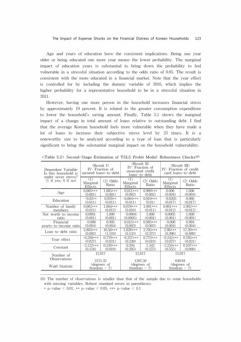
With respect to the high correlation between a loan with the total debt
outstanding, Table 5.2 presents the results from the two stage instrumental
variable probit model. In this regression, the debt is fitted by the fraction of each
loan and other demographic variables (which are assumed as exogenous ones) and
then plugged into the second stage regression of estimating its marginal impact on
the stress. In Table 5.2, the TSLS results are presented according to the
instrumental variable for the loan-to-debt ratio. Specifically, for each estimation, I
use the first stage results on the estimated loan-to-debt ratio that is fitted by the
fraction of secured loans-to-debt in (Result I), the fraction of unsecured
loans-to-debt in (Result II), and finally the fraction of credit card loans-to-debt in
(Result III). For each estimation of the loan-to-debt ratio, the demographic
variables and other flow variables are controlled.
With the smaller degrees of freedom, the results show that the baseline
random-effects probit estimation is valid to emphasize the different effect by a
loan category. Although the statistical significance, and sign of an impact are
consistent with them from the probit model. there are some changes in the size of
the coefficient. For example, the impacts of the financial-asset-to-income ratio and
the debt-to-income ratio significantly increase. On the other hand, the number of
family members and years of education show a smaller impact on the stress.
The marginal impacts of other variables are consistent with those shown in
Table 5.1. Further, as discussed, the impact of loan-to-debt ratio can be different
when it is estimated by a different type of loan. For example, when the ratio is
instrumented by the fraction of secured loans-to-debt amount, it impacts on the
probability of household’s being under a sever stress to increase it by 16.5 times
greater than when it has not made a secured loan. The impact’s size of
loan-to-debt ratio is shown to be similar when it is instrumented by the credit
card loans (including cash advances, revolving accounts, and installment payment)
to report its marginal effect by 2.86 at 0.01% significant level. In summary, when
a household is afraid of that she cannot to repay loans through easily revolving,
but expensive, cost-based credit card loans, her stress indicates a severe stress.
On the other hand, all else constant, the odds ratio is 2.795 when a household
delivers money through unsecured credit loans, which are not related to credit
cards.
Table 5.3 presents the first-stage estimation results of the TSLS probit model.
Regarding the marginal impact of a specific loan, in general, the loan-to-debt ratio
is in a positive relationship with all types of loans. When the loan-to-debt ratio is
regressed on the fraction of secured loans-to-debt, it tends to increase by 34
percent when there is a unit increase in the fraction. Interestingly, although the
marginal impact of the fraction, which is obtained by the credit card loans-to-debt

The Impact of Expense Shocks on the Financial Distress of Korean Households 125
ratio, is only 20 percent, the loan-to-debt ratio in the first stage brings a
significant change in a household’s subjective probability of being under stress (by
2.86 at the marginal effect, Result III of Table 5.2). In other words, for the
households of who are exposed at a high possibility to be vulnerable, the credit
card loans could be critical at margin in spite of its small impact on the
aggregate loan among debt.
<Table 5.3> First-Stage Estimation of TSLS Probit Model11)
Dependent Variable = Loan-to-debt ratio Marginal Effects Marginal Effects Marginal Effects
Age -0.0088***(0.0002)
-0.0085***(0.0003)
-0.0088***(0.0003)
Education -0.035***(0.002)
-0.0312***(0.002)
-0.0334***(0.0025)
Number of family members
-0.0033(0.002)
0.0113**(0.003)
0.0109***(0.0026)
Net worth-to-income ratio
-0.0005***(0.0001)
-0.0003***(0.0001)
-0.0004***(0.0001)
Financial assets-to-income ratio
-0.006***(0.0006)
-0.005***(0.0007)
-0.0051***(0.0008)
Fraction of secured loans to debt
0.338***(0.007) - -
Fraction of unsecured loans to debt - 0.2545***
(0.0085) -
Fraction of credit card loans to debt - - 0.2002***
(0.0180)
Year effect -0.006(0.0057)
-0.0080(0.0061)
-0.009(0.0063)
Constant 1.255***(0.0214)
1.276***(0.023)
1.35***(0.024)
Number of Observations,
Adjusted R-squared
12,017
0.2605(degrees of freedom = 7)
12,017
0.1585(degrees of freedom = 7)
12,017
0.1048(degrees of freedom = 7)
Table 5.4 provides more specific, but the consistent information about the
factors. More specifically, EWS results show that Korean households feel
11) The number of observations is smaller than that of the sample due to some households
with missing variables. Robust standard errors in parentheses.
* p-value < 0.01, ** p-value < 0.05, *** p-value < 0.1

126 Jane Yoo
vulnerable when their financial debt approaches 4,190 thousands won per household
in a year, which is responsible for a debt-to-income ratio of 213 percent. The
threshold ratio provides the valuable information, which cannot be captured by the
level of debt and income separately owing to outliers with the extreme
debt-to-income ratio. The optimal split of the debt-to-net worth ratio is lower in
Korea where most households hold non-financial assets in home equity value (the
threshold is 19 percent level of the debt-to-net worth ratio). These debt-related
ratios imply a predictive power of between 59 and 75 percent.
To develop an efficient screening procedure, I finally examine the goodness of
fit for all indicators and conclude that the financial debt-to-financial assets ratio
(with the optimal threshold of 24.22 percent), the debt-to-income ratio (the
threshold of 213 percent), the outstanding debt (the threshold of 4,190 thousands
won), and the debt-to-net worth ratio (the threshold of 19 percent) are significant.
In this analysis, the proportion of unsecured credits to the total amount of
household loans turns out the sensitive one to show a level of vulnerability.
However, savings, assets, net worth, income, expenditure, and the proportion of
secured loans may not be sensitive indicators at margin because most households
in Korea already own housing assets and use earning wages and salaries to
maintain consumption. The results of the present study thus emphasize that
lenders should pay particular attention to credit card usage or unsecured credit
when investigating a borrower’s willingness and ability to repay debt.
Furthermore, this criteria could be an efficient one for policymakers when they
find an appropriate indicator to reduce the household financial distress level and
credit-related vulnerabilities.

The Impact of Expense Shocks on the Financial Distress of Korean Households 127
<Table 5.4> Baseline Optimal Split and Goodness of Fit
by an Early Warning Signal Method12)
Variable
(1)
Optimal
Split
Value
(2) Proportion of
a stress indicator
missed
(3) Proportion of
non-stress
indicators
called in error
(4) Goodness of Fit
Financial debt-to-
financial assets ratio 24.22% 0.032 0.216 0.7524
Debt-to-
income ratio 213% 0.034 0.326 0.6399
Debt 419 0.02878 0.337 0.6342
Debt-to-net worth
ratio 19% 0.118 0.287 0.5949
Proportion of
(unsecured) credits 0.0034% 0.559 0.247 0.1938
Proportion of
credit card usage 0% 0.791 0.094 0.1151
Savings 576 0.137 0.783 0.0802
Financial assets 847 0.152 0.784 0.0646
Net worth -0.5513) 0.927 0.009 0.0644
Disposable income 536.61 0.113 0.870 0.0173
Daily expenses 1.66 0.036 0.960 0.0072
Home equity value 95.15 0.020 0.975 0.0048
Income 913.03 0.055 0.942 0.0034
Proportion of
secured loans 100% 0.001 0.998 0.0004
12) Source: Author’s calculation obtained by the early warning signal method. Indicators are
sorted by their absolute goodness of fit to truly call household financial distress. The
optimal split values of flow variables are in ten thousand Won. See text for more details
in estimation.
13) The negative value of the optimal threshold is related to the debt-to-net worth ratio,
which is higher than 100%. In other words, some households could maintain a budget
free from the financial stress even when they have more debt than assets. This is
consistent with the findings with the U.S household data.

128 Jane Yoo
5.2 Estimation of expense shocks
Our major findings about expense shocks are presented in Table 5.5 and 5.7.
For each type of loan, the impacts of expense shocks are explained after age,
years of education, number of family members, net worth, and outstanding debt
are controlled. All flow variables except years of education are normalized by
taking its ratio relative to income. The model also controls for the year effect by
including the 2010-year dummy variable as before. In this paper, we present the
results with the sample of households who do have loans or debts: all variables
except demographic ones are a natural log transformed. The results are significant
with the results with the whole sample or without the transformation and the
results are available from authors upon request.
All demographic variables examined with expense shocks delivered through
secured and unsecured debt are significant in line with the previous model. No
matter what type of loan is used, the number of family members and years of
education are significant to increase the probability of being in the stress. The
size of the marginal effect increases particularly when a household use credit card
loans according to their odd ratios (1.457 for the number of family members; 1.343
for the debt-to-income ratio).
Although the probability of having the stress is lowered when a household has
more net worth (by 2.2 percent) or financial assets (by 5.1 percent) relative to
income particularly when they use a secured borrowing channel, it implies the
different meaning for a household with unsecured credits including credit cards.
More specifically, the impact of net worth decreases for the households with
unsecured credits in contrast to that of financial assets is more significant (by
15.4 percent). Moreover, their effects are not significant or negligible for a
household whose borrowing is based on credit card loans. Interestingly, the credit
card loans may give the significant stress when a household uses a card for
rental payment, (the odd ratio of 1.024), debt repayment (1.026). On the other
hand, if those loans are used for business management the household stress level
decreases by 1.8 percent. (the odd ratio of 0.982). The decrease in the
business-owners’ vulnerability is explained by some entrepreneurs with the
substantial amount of business equities/assets to prove their creditworthiness. The
evidence is consistent with the results from other types of loans; no matter what
type of loan is financed, a business-owner household is relatively free from
stresses even when they borrow. These expenses are more closely related with
investment costs that a household expects a good income stream.
For households who have borrowed money either through a secured channel or
through unsecured one, some situations are stressful: home-financing, medical

The Impact of Expense Shocks on the Financial Distress of Korean Households 129
expenses, educational expenses, and daily expenses. Here, daily expenses contain
the daily consumption expenditure on general food and service items.
Subsequently, if a household needs to borrow money for this particular aim, she is
highly likely to belong the low income quintile. The expense shocks that arise
from financing non-home equities and miscellaneous cases are omitted to avoid
the nearly perfect multicollinearity with other explanatory variables. Particularly, it
is interesting to find the medical expenses to increase the household financial
stress because it means the double burden for her from i) a large amount of
sudden expenditure; ii) a potentially sudden stop of labor income stream if a
household head is not able to work any more by hospitalization.
<Table 5.5> Probit Model by Expense shock14)
Variables Secured Debt Unsecured Credit Credit Card Debt (1) Marginal
Effects (2) Odds
Ratio (3) Marginal
Effects (4) Odds
Ratio (5) Marginal
Effects (6) Odds
Ratio
Age -0.0163***
(0.004) 0.984***(0.004)
-0.021***(0.005)
0.979***(0.005)
-0.019(0.015)
0.981(0.015)
Years of education
-0.260*** (0.0312)
0.771***(0.024)
-0.290***(0.039)
0.748***(0.029)
-0.258**(0.129)
0.773**(0.1)
The number of family members
0.115*** (0.034)
1.122***(0.038)
0.146***(0.039)
1.157***(0.045)
0.376***(0.136)
1.457***(0.198)
Debt-to-income ratio
0.236***(0.0189)
1.266***(0.024)
0.316**(0.028)
1.371***(0.039)
0.295***(0.081)
1.343***(0.109)
Net worth-to-income ratio
-0.022***(0.004)
0.978***(0.004)
-0.0302***(0.006)
0.970***(0.006)
0.006(0.023)
1.006(0.023)
Financial asset-to-income ratio
-0.051***(0.0161)
0.950***(0.015)
-0.154***(0.025)
0.858***(0.022)
-0.087(0.059)
0.917(0.054)
Debt used For: Home financing
0.0063***(0.001)
1.006***(0.001)
0.005*(0.002)
1.005*(0.002)
-0.0153(0.014)
0.985(0.014)
Debt used For: Rental payment
0.0058***(0.002)
1.006***(0.002)
0.0068**(0.002)
1.007***(0.002)
0.023**(0.012)
1.024**(0.012)
Debt used For: Stock investment
0.00173(0.0043)
1.002(0.004)
-0.003(0.004)
0.997(0.004)
-0.015(0.0105)
0.985(0.014)
Debt used For: Debt repayment
0.0123***(0.003)
1.012***(0.003)
0.012***(0.003)
1.012***(0.003)
0.026**(0.011)
1.026**(0.011)
Debt used For: Business management
-0.009***(0.0013)
0.991***(0.001)
-0.008***(0.002)
0.992***(0.002)
-0.017***(0.006)
0.982***(0.006)
Debt used For: Wedding expense
0.0067**(0.003)
1.007***(0.003)
-0.0004(0.004)
1(0.004)
0.205(180.7)
1.227(221.7)
Debt used For: Medical expense
0.017***(0.005)
1.017***(0.003)
0.011***(0.004)
1.011***(0.004)
0.0001(0.008)
0.999(0.008)
Debt used For: Educational expense
0.007***(0.003)
1.007***(0.003)
0.004*(0.002)
1.004*(0.002)
0.006(0.007)
1.006(0.007)
Debt used For: daily expenses
0.008***(0.002)
1.008***(0.002)
0.005***(0.002)
1.005***(0.002)
0.002(0.005)
1.002(0.005)
Year effect -0.716***(0.072)
0.489***(0.035)
-0.780***(0.091)
0.458***(0.042)
-0.866***(0.28)
0.420***(0.118)
Observations 6,749 4,409 1,301 Pseudo R-squared 0.1358 0.1637 0.1469
14) The number of observations is smaller than that of the sample due to some households
with missing variables. Robust standard errors in parentheses.
* p-value < 0.01, ** p-value < 0.05, *** p-value < 0.1

130 Jane Yoo
Variables
Secured Debt Unsecured Credit Credit Card Debt
VIFSQRTVIF
Tolerance
VIFSQRTVIF
Tolerance
VIFSQRTVIF
Tolerance
Age 1.39 1.18 0.7216 1.34 1.16 0.7469 1.23 1.11 0.8123
Years of education 1.30 1.14 0.7713 1.32 1.15 0.7549 1.20 1.09 0.8350
The number of family members
1.10 1.05 0.9128 1.08 1.04 0.9286 1.08 1.04 0.9260
Debt-to-income ratio
1.39 1.18 0.7203 1.44 1.20 0.6935 1.05 1.02 0.9538
Net worth-to-income ratio
1.64 1.28 0.6092 1.47 1.21 0.6817 1.24 1.11 0.8090
Financial asset-to-income ratio
1.26 1.12 0.7945 1.07 1.04 0.9329 1.15 1.07 0.8692
Debt used For: Home financing 2.32 1.52 0.4303 1.49 1.22 0.6707 1.08 1.04 0.9293
Debt used For: Rental payment
1.59 1.26 0.6291 1.71 1.31 0.5838 1.35 1.16 0.7429
Debt used For: Stock investment
1.04 1.02 0.9584 1.11 1.06 0.8979 1.14 1.07 0.8775
Debt used For: Debt repayment
1.19 1.09 0.8382 1.44 1.20 0.6959 1.58 1.26 0.6316
Debt used For: Business management
1.81 1.34 0.5532 2.65 1.63 0.3772 2.13 1.46 0.4686
Debt used For: Wedding expense
1.11 1.05 0.8988 1.10 1.05 0.9118 1.03 1.01 0.9722
Debt used For: Medical expense
1.07 1.03 0.9385 1.21 1.10 0.8261 1.32 1.15 0.7597
Debt used For: Educational expense
1.16 1.08 0.8630 1.70 1.30 0.5872 1.66 1.29 0.6036
Debt used For: daily expenses 1.61 1.19 0.7094 2.91 1.71 0.3440 3.17 1.78 0.3151
Year effect 1.01 1.00 0.9928 1.00 1.00 0.9916 1.01 1.01 0.9890
Mean VIF 1.36 1.50 1.40
With respect to the near-multicollinearity between the fractions, which indicate
the particular reason of borrowing, Table 5.6 presents the collinearity diagnostics
on a probit model by the expense shock. Tolerance, defined as 1/VIF, is used by
many researchers to check on the degree of collinearity. In Table 5.6, there is no
indicator with a tolerance value lower than 0.1 (it is comparable to a VIF of 10).
It means that the variable is not considered as a linear combination of other
independent variables.
<Table 5.6> Collinearity Diagnostics on Probit Model by Expense shock

The Impact of Expense Shocks on the Financial Distress of Korean Households 131
Variable
(1) Number of Stress indicator Observati
ons
(2) Total Number of
Non-Missing Observations
(3) Proportion of a severe
stress missed
(4) Proportion of
non-stress called
in error
(5) Goodness of
Fit
ln(credit cards: medical expense) 33 40 0.364 0 0.636
ln(credit cards: stock investment)
12 18 0.333 0.167 0.5
ln(credit loans: wedding expense)
35 50 0.457 0.133 0.410
ln(secured loans: daily expenses)
526 619 0.317 0.333 0.349
ln(credit cards: rental payment)
41 43 0.659 0 0.341
ln(credit cards: daily expenses) 680 778 0.335 0.327 0.338
ln(secured loans: educational expense) 203 248 0.429 0.289 0.283
ln(credit loans: stock investment)
33 57 0.394 0.333 0.273
ln(credit loans: medical expense)
90 104 0.267 0.5 0.233
ln(credit loans: daily expenses)
1319 1636 0.357 0.416 0.227
ln(secured loans: home) 2425 2985 0.509 0.279 0.213
Table 5.7 supports the evidences suggested in Table 5.5. In the EWS analysis,
the top three expense shocks, namely credit card loans for medical expenses, risky
investments in stocks, and unsecured loans for wedding-related expenses.
Although they affect a small proportion of the population, they are efficient to call
stresses: they are at the moment of loaning money for these objectives is crucial
for household to cover emergency costs. The predictive power of the other types
of loans in resolving expense shocks are too close to be narrowed to a set of
informational indicators. However, in general, loans secured by equities are ranked
highly as their loan amount endogenously fluctuates with the collateral value.
When the collateral value changes over the business cycle, a debt limit or
leverage is constrained, regardless of whether personal productivity restricts
consumption. This makes households feel vulnerable to an unexpected expense
shock.
<Table 5.7> Goodness of Fit of the Expense shock in an Early Warning Signal
Model15)
15) Source: Author’s calculation obtained by the early warning signal method. Indicators are
sorted by their absolute goodness of fit to truly call household financial distress. See text
for more details in estimation.

132 Jane Yoo
ln(secured loans: stock purchase) 41 58 0.683 0.118 0.199
ln(secured loans: wedding expense)
97 119 0.227 0.591 0.182
ln(credit cards: educational expense) 83 93 0.831 0 0.169
ln(credit loans: debt repayment) 243 273 0.654 0.2 0.146
ln(secured loans: business)
780 1232 0.490 0.372 0.139
ln(secured loans: debt repayment)
242 272 0.533 0.333 0.134
ln(secured loans: medical expense)
66 73 0.727 0.143 0.130
ln(secured loans: rental payment)
534 676 0.788 0.085 0.127
ln(credit loans :educational expense) 347 444 0.591 0.299 0.110
ln(credit loans: business management) 705 1106 0.343 0.554 0.103
ln(credit cards: business management)
121 166 0.322 0.578 0.100
ln(credit loans: rental payment)
310 390 0.187 0.775 0.038
ln(credit loans: home) 215 264 0.884 0.082 0.035
ln(credit cards: debt repayment)
85 87 0 1 0
5.3 Robustness checks
This section has two aims, to verify the robustness of the estimation results,
and to confirm the usefulness of the EWS methodology in screening household
financial health. Table 5.8 presents the correlation between the vulnerability flags
predicted by various estimation. If these predictions have a high correlation with
the real stress index, the estimation results are robust and useful to examine a
household’s financial health in the future studies. In the examination, I compare
the factor, EWS, and logit models. Factor analysis can explain data in the form of
few variables because it finds a few common factors that linearly reconstruct the
matrix made by the original explanatory variables. In this process, the model finds
the diagonal matrix of uniqueness by computing the leading eigenvectors, scaled
by the square root of the appropriate eigenvalue. Under a factor model, the system
of regression equations are established by the factor-loaded variables matrix.
The predicted flags are compared with the actual financial distress index. I find
that the flag raised by the EWS has a 69 percent correlation with actual
delinquency reports, which is lower than that of the factor regression models, but
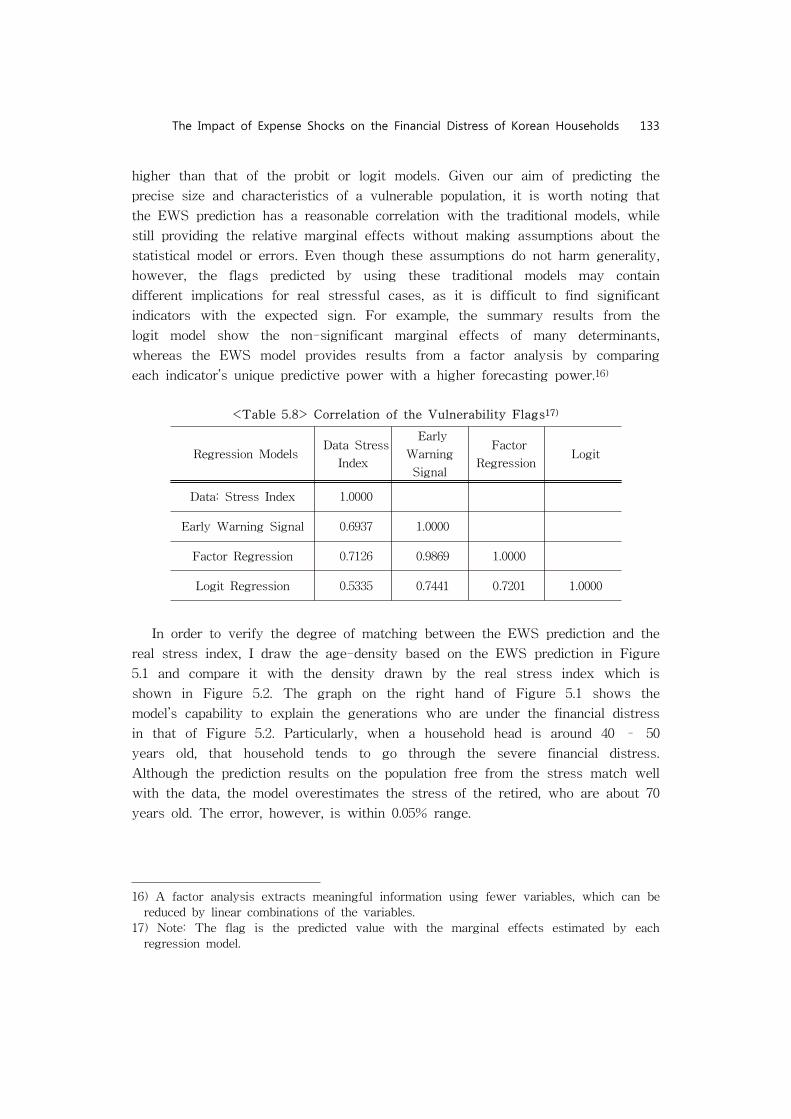
The Impact of Expense Shocks on the Financial Distress of Korean Households 133
higher than that of the probit or logit models. Given our aim of predicting the
precise size and characteristics of a vulnerable population, it is worth noting that
the EWS prediction has a reasonable correlation with the traditional models, while
still providing the relative marginal effects without making assumptions about the
statistical model or errors. Even though these assumptions do not harm generality,
however, the flags predicted by using these traditional models may contain
different implications for real stressful cases, as it is difficult to find significant
indicators with the expected sign. For example, the summary results from the
logit model show the non-significant marginal effects of many determinants,
whereas the EWS model provides results from a factor analysis by comparing
each indicator’s unique predictive power with a higher forecasting power.16)
<Table 5.8> Correlation of the Vulnerability Flags17)
Regression Models Data Stress
Index
Early
Warning
Signal
Factor
Regression Logit
Data: Stress Index 1.0000
Early Warning Signal 0.6937 1.0000
Factor Regression 0.7126 0.9869 1.0000
Logit Regression 0.5335 0.7441 0.7201 1.0000
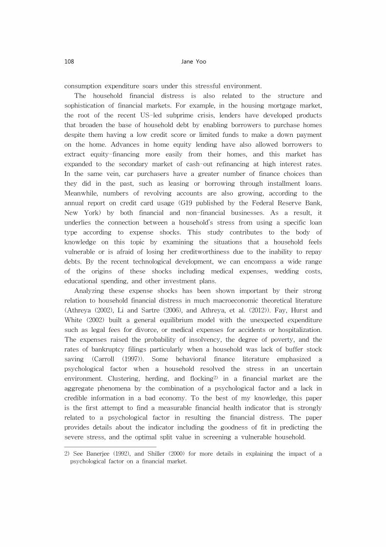
In order to verify the degree of matching between the EWS prediction and the
real stress index, I draw the age-density based on the EWS prediction in Figure
5.1 and compare it with the density drawn by the real stress index which is
shown in Figure 5.2. The graph on the right hand of Figure 5.1 shows the
model’s capability to explain the generations who are under the financial distress
in that of Figure 5.2. Particularly, when a household head is around 40 – 50
years old, that household tends to go through the severe financial distress.
Although the prediction results on the population free from the stress match well
with the data, the model overestimates the stress of the retired, who are about 70
years old. The error, however, is within 0.05% range.
16) A factor analysis extracts meaningful information using fewer variables, which can be
reduced by linear combinations of the variables.
17) Note: The flag is the predicted value with the marginal effects estimated by each
regression model.

134 Jane Yoo
<Figure 5.1> Comparison of the estimated kernel age density between household
with and without the financial stress from the EWS estimation18)
<Figure 5.2> Comparison of the empirical kernel age density between household
with and without the financial stress from the survey of household finance19)
18) Source: Author’s calculation using the survey of household finance in 2010 and 2011.
The kernel density is obtained by the fitted sample population over a household head’s
age. After sorting the major determinants from an early warning signal method according
to the goodness of fit, I examine whether a component of each household’s balance sheet
is over/under the indicator’s optimal threshold. The weight on an indicator allows us to
determine which indicator is more valuable in sorting out the vulnerability of a household.
Finally, the age density is drawn by this examination, not by the subjectively measured
financial stress, with a gaussian kernel
19) Source: The survey of household finance in 2010 and 2011. The kernel density indicates
The Impact of Expense Shocks on the Financial Distress of Korean Households 135
6. Conclusion
This study examined the specific expense shocks that are strongly linked to
the financial distress of Korean households. Accoridng to the bootstrapped random
effect probit model and EWS estimation, some expenses, particularly medical and
miscellaneous daily expenses through unsecured and credit card loans, significantly
influence household distress: when a household is using these loans, it is highly
likely that they feel to fail in repaying debt on schedule. The main results are
The results of the EWS model suggest that the following three sudden expense
shocks explain a substantial degree of household vulnerability: i) secured loans for
debt repayment, medical expenses, and daily expenses; ii) unsecured credits for
debt repayment, medical expenses and rents; iii) credit card loans for debt
repayment, and rents.
Based on these results, this study suggests that the study then develops a
screening tool that could be used before implementing a public policy that targets
the relief of certain types of debts. Further, it aims at diminishing credit risks in
the economy. A specific threshold level and goodness of fit of the indicators are
also found by the EWS model. Policy makers that aim to provide debt relief
should thus consider establishing a social safety net to help mitigate these
expense shocks. Indeed, the results of the presented analysis imply that it is more
important for policy makers to understand the source of expense shocks rather
than the source of funds if their main objective is to implement an efficient and
effective preemptive strategy to diminish household financial distress. This work,
however, is limited to panel data in 2010 and 2011 in South Korean households
(the Survey of Household Finance). Expanding the dataset would allow researchers
to analyze the impact of expense shocks on the probability of bankruptcy by
considering the household dynamics of lifetime income, consumption, and wealth.
(2014년 1월 3일 수, 2014년 2월 13일 수정, 2014년 3월 26일 채택)
Acknowledgement
This work was (partially) supported by the new faculty research fund of Ajou
University. An author appreciate the valuable comments from three unknown
referees, Jung-soon Shin, and Jun-ho Hahm. All remaining errors are my own.
the age density according to the level of financial distress, which is reported by a
household’s head in the survey.

136 Jane Yoo
References
Athreya, K. B. (2002). Welfare implications of the bankruptcy reform act of 1999.
The Journal of Monetary Economics, 49(8):1567-1595.
Attanasio, O., Banks, J., Meghir, C., and Weber, G. (1999). Humps and bumps in
lifetime consumption. The Journal of Business & Economic Statistics,
17(1):22-35.
Attanasio, O. P. and Browning, M. (1995). Consumption over the life cycle and
over the business cycle. The American Economic Review,
85(5):1118-1137.
Banerjee, A. J. (1992). A simple model of herd behavior. The Quarterly Journal of
Economics, 107(3):797-817.
Bornsztein, E., and Pattillo, C. (2005). Assessing early warning systems: How have
they worked in practice?. IMF Staff Papers, 52(3):462-502.
Carroll, C. D. (1997). Buffer-stock saving and the life cycle/permanent income
hypothesis. The Quarterly Journal of Economics, 112(1):1-55.
Dawsey, A. E. and Ausubel, L. M. (2004). Informal bankruptcy. Working paper.
Domowitz, I. and Sartain, R. L. (1999). Determinants of the consumer bankrtupcy
decision. The Journal of Finance, 54(1):403-420.
Fay, S., Hurst, E., and White, M. J. (2002). The household bankrtupcy decision.
The American Economic Review, 92(3):706-718.
Fernandez-villaverde, J. and Krueger, D. (2011). Consumption and saving over the
life cycle: How important are consumer durables?. Macroeconomic
Dynamics, 15(5):725-770.
Ghosh, A. R., Crowe, C., Kim, J. I., Ostry, J. D., and Chamon, M. (2011). Imf
policy advice to emerging market economies during the 2008-2009 crisis:
New fund or new fundamentals?. The Journal of International
Commerce, Economics and Policy, 2(1):1-17.
Ghosh, S. R. and Ghosh, A. R. (2003). Structural vulnerabilities and currency
crises. IMF Staff papers, 50(3).
Gourinchas, P.-O. and Parker, J. A. (2002). Consumption over the life cycle.
Econometrica, 70(1):47-89.
Gross, D. B. and Souleles, N. S. (2002). An empirical analysis of personal
bankruptcy and delinquency. The Review of Financial Studies,
15(1):319-347.
Kaminsky, G., Lizondon, S., and Reinhart, C. M. (1998). Leading indicators of
currency crises. IMF Staff Papers, 45(1):1-48.
Kim, B. S. and Jeon, H. C. (2000). Trend and implications of the recent personal
bankruptcy. Samsung Economic Research Institute.

The Impact of Expense Shocks on the Financial Distress of Korean Households 137
Kim, D.-w. and Kim, K. (2010). The stress test of household loan sector
considering heterscedasticity, autocorrelation and conditional loss at
given default. Quarterly Bulletin, the Bank of Korea, 16(3):119-155.
Kim, K. (2012). Role of financial factors in korean business cycle. The Korean
Journal of Economics, 19(1):177-212.
Kim, K. and Lee, C.-s. (2012). Household delinquency index and household debt.
LG Economic Research Institute, March: 2-18.
Kim, Y. S., Ha, J. L., and Kim, J. H. (2009). Measurement and evaluation of credit
risk of the financial system by using debtor's repayment capability.
Monthly Bulletin, the Bank of Korea, December: 24-55.
Lee, C. S. (2012). Portfolio of household assets: exposed to higher volatility risks
in a housing market. LG Economic Research Institute, February: 2-13.
Lee, C. S. and Kim, K. (2012). Measuring the household credit risk using stress
test. LG Economic Research Institute, August: 2-17.
Lee, J. H. and Jeong, H. Y. (2005). An empirical study on improvement of credit
scouring system in the credit loan of household from bank. Korean
Academic Society of Accounting, (4):55-73.
Li, W. and Sarte, P.-D. (2006). U.S. consumer bankruptcy choice: The importance
of general equilibrium effects. The Journal of Monetary Economics,
53(3):613-631.
Manasse, P., Roubini, N., and Schimmelpfennig, A. (2003). Predicting sovereign
debt crises. IMF Working Paper 03/221.
Park, I., Kwon, D., Yun, T., Cho, J., and Shim, H.-R. (2012). Analysis on the risk
of household debts by financial services sector. Kis Rating,
September:4-37.
Shiller, R. J. (2000). Irrational exuberance. Princeton University Press.