91

5. STATISTICS OF LANDSLIDE SIZE

Somehow you need years to recognize something obvious.

Not all what can be counted counts, and

not all what counts can be counted.

The size (e.g. length, area, volume) of individual landslides varies largely. As shown in Figure 1.1, the length of landslides varies from less than a meter to several hundreds or even thousands of kilometres for submarine slides. Landslide area spans the range from less than a few square meters, for shallow soil slides, to thousands of square kilometres, for large submarine failures. The volume of single mass movements ranges from less than a cubic decimetre, for rock fragments falling off a cliff, to several hundreds of cubic kilometres, for gigantic submarine slides (Locat and Mienert, 2003), or for slope failures identified on the Moon (Hsu, 1975), Mars (McEwen, 1989) and Venus (Malin, 1992).

The frequency-size distribution of landslides is important information to determine landslide hazards (Guzzetti et al., 2005a) (see § 7.3), and to estimate the contribution of landslides to erosion and sediment yield (e.g., Hovius et al., 1997, 2000; Martin et al., 2002; Guthrie and Evans, 2004b; Lavé and Burbank, 2004). For these reasons, it is essential that the distributions are quantified precisely, using accurate and reliable methods.

In this chapter, after a review of the limited literature, I show how to obtain frequency-area and frequency-volume statistics of landslides from empirical data obtained from landslide inventories. I then discuss applications of the obtained frequency statistics of landslides, with examples from the Umbria region, including an application to investigate the completeness of the three landslide inventory maps available for the Collazzone area.

5.1. Background

Review of the literature (§ 13) reveals that only a few authors have investigated the frequency-area, or the frequency-volume statistics of landslides. Fujii (1969) was probably the first to investigate the problem. Studying an inventory of 800 landslides caused by heavy rainfall in Japan, he obtained a cumulative number-area distribution that correlated well with a power law relation of the type α−∝ LCL AN , where NCL is the cumulative number of landslides, AL is the landslide area, and α = 0.96. This author also obtained a similar cumulative number-volume distribution that correlated with a power law α−∝ LCL VN , with VL the landslide volume and α = 0.85. Other investigators have studied the frequency-size distribution of landslides in Japan. Ohmori and Hirano (1988) examined 3511 landslides occurred in the 8-year period

Statistics of landslide size

92

between 1975 and 1983, and provided cumulative number-area distributions that correlated with power laws with exponents α in the range between 1.34 and 1.62, depending on the type of the mapped landslides. Sugai et al. (1994) and Ohmori and Sugai (1995) examined 3424 landslides in the Akaishi Ranges, in central Japan, and found power law correlations for landslides in different rock types and elevation zones with values of α in the range from 1.27 to 2.49. Sasaki et al. (1991) investigated the width of landslides triggered by heavy rainfall in the Misumi and Masuda areas, in south western Japan, and found a relationship between the cumulative number of landslides and the maximum width of the slope failures that was approximated by a power law with an exponent α ~ 3.3.

Pelletier et al. (1997) have given cumulative frequency-area distributions of rainfall induced landslides in Japan and in Bolivia, and of earthquake induced landslides in California. The data set for Japan was the same compiled by Sugai et al. (1994) for the Akaishi Ranges described before. For this data set, Pelletier et al. (1997) found a power law relation between the area of the landslides and the cumulative number of slope failures with an exponent α = 2.0, for slope failures larger than about 1×105 m2. The data set for Bolivia was compiled by Blodgett (1998), who mapped 1130 rainfall induced landslides in the Challana Valley, in the Eastern Cordillera. For this data set, Pelletier et al. (1997) found power law relationships with exponents ranging between α = 1.6 and α = 2.0, for landslides larger than about 5×104 m2. The data set for California consisted in about 11,000 landslides triggered by the 17 January 1994 Northridge earthquake and mapped by Harp and Jibson (1995, 1996). For this data set, the cumulative distribution of landslide areas was approximated by a power law taking the slope α = 1.6, for landslides larger than about 3×103 m2. Malamud and Turcotte (1999) analysed the same data sets used by Pelletier et al. (1997), and another data set listing 709 landslides mapped by Nielsen et al. (1975) for the Eden Canyon area in Alameda County, California. The obtained non-cumulative frequency-area distributions exhibited a “rollover” for landslides areas smaller than about 2×103 ~ 1×104 m2, depending on the resolution of the mapping, and were all reasonably well approximated by power laws with exponents, α+1, in the range between 2.3 and 3.3.

Hovius et al. (1997) have given a cumulative number-area distribution for 4984 landslides mapped in a mountain area east of the Alpine fault in New Zealand. Their logarithmically binned data correlated with a power law relation with α = 0.7, over the range AL = 7×102 m2 to AL = 1×106 m2. Hovius et al. (2000) have given a number-area distribution of 1040 fresh landslides in the Ma-An and Wan-Li catchments on the eastern side of the Central Range in Taiwan. The logarithmically binned data correlated with a power law relation with exponent α = 1.15 over the range AL = 1×103 m2 to AL = 5×104 m2. Stark and Hovius (2001) revised the given number-area distributions obtained for southern New Zealand and central Taiwan. The revised estimates were obtained by fitting non-cumulative distributions of the available data to cover the mapped landslide areas, a significant improvement over pre-existing published work. For the purpose, the authors introduced a five parameters double-Pareto distribution (§ 5.2.1, equation 5.3), and obtained estimates for the slope of the power law tail of the distribution of α+1 = 2.11 for the Taiwan inventory, and α+1 = 2.46±0.2 for the New Zealand inventory.

Various authors have examined the frequency-area distributions of landslides in British Columbia, Canada. Martin et al. (2002) studied 615 landslides in the Queen Charlotte Islands, which ranged in area from 200 to 52,000 m2, and spanned the volume from 217 m3 to 16,100 m3. The non-cumulative probability-density distributions for landslide areas were approximated by power laws with exponents α+1 = 1.80, for primary landslides, and α+1 = 3.20 for gully sidewall events. Guthrie and Evans (2004b) analyzed three inventories showing

Chapter 5

93

landslides occurred on the west coast of British Columbia. The first inventory listed 201 debris slides and debris flows, 136 of which occurred in the 47-year period from 1950 to 1996, in a 286 km2 study area in the Brooks Peninsula. The second inventory listed 92 landslides in the Loughborough Inlet. The third inventory showed 1109 landslides inventoried by the British Columbia Ministry of Forest in the Clayoquot study area. The mapped landslides ranged in size from 500 m2 to 400,000 m2, and their non-cumulative frequency-area distributions obeyed power law relationships with exponents α+1 ranging between 2.51 and 2.77, for landslide areas ranging from AL = 1×104 m2 to AL = 4×105 m2. In another paper, Guthrie and Evans (2004a) have given the frequency-area statistics for 101 rainfall-induced landslides occurred on 18 November 2001 in the Loughborough Inlet, a slightly different data set than then one used in the previous paper. These landslides ranged in size from 1124 m2 to 409,000 m2, and their frequency-area distribution was described by a power law with a slope α+1 = 2.24, for landslides larger than ~1×104 m2. Guthrie and Evans (2004a,b) argued that the rollover shown in their non-cumulative distributions was real, and not an artefact due to under-sampling of the landslides. Brardinoni and Church (2004), working in the Capilano coastal watershed in British Columbia, have determined that in this area the rollover occurs for landslides greater than about 4000 m3.

Guzzetti et al. (2002) have given non-cumulative frequency-area distributions for two landslide data sets in central Italy. The first data set consisted of 16,809 landslides in the Umbria and Marche area. These landslides were originally mapped by Guzzetti and Cardinali (1989) (§ 3.3.2.1) and by Antonini et al. (1993) through the interpretation of medium-scale aerial photographs and limited field checks. The second data set consisted in 4233 landslides triggered by rapid snow melting in Umbria on 1 January 1997 (§ 3.3.3.2). The two data sets exhibited distinct rollovers for the smallest mapped landslides, and were found to correlate well with a power law relation with exponent α+1 = 2.5 for the largest landslides, albeit for different (but overlapping) ranges: i.e., AL = 3×104 m2 to AL = 4×106 m2 for the reconnaissance geomorphological mapping, and AL = 1×103 m2 to AL = 1×105 m2 for the event inventory. Guzzetti et al. (2002) argued that the rollover for small landslide areas shown in the non-cumulative distributions had different explanations. The rollover shown in the reconnaissance inventory was attributed to incompleteness of the landslide record due to erosion and to limitations in the reconnaissance mapping technique used to compile the inventory, whereas the rollover in the event inventory was considered real, and possibly associated with the surface morphology or the landslide process itself. Guzzetti et al. (2004a) examined an inventory of 1204 landslides triggered by intense rainfall on 23 November 2000 in the Imperia Province, northern Italy. In this inventory, landslides ranged in size from 50 m2 to 7×104 m2, for a total landslide area of 1.6 km2. The obtained non-cumulative probability density of landslide areas exhibited two features typical of landslide-area distributions, namely, (i) the distribution had a distinct power law tail with an exponent α+1 = 2.5, and (ii) the distribution exhibited a distinct rollover for the smaller landslide areas, showing that a characteristic size existed for which landslides were most abundant in the study area.

Guzzetti et al. (2005a) have estimated the non-cumulative probability density distribution for 2390 landslides occurred in the 45-year period from 1955 to 1999 in the Staffora River basin, in the northern Apennines of Italy. The landslide information used to determine the probability density of landslide areas was obtained from the multi-temporal inventory described in § 2.6. The obtained probability density of landslide areas obeys a power law relation for landslide areas in the range from 5×103 m2 to 2×105 m2, and exhibits a distinct rollover for landslides smaller than 1.5×103 m2. To obtain the probability density, Guzzetti et al. (2005a) used the

Statistics of landslide size

94

double-Pareto distribution of Stark and Hovius (2001) (equation 5.3) and the truncated inverse Gamma distribution of Malamud et al. (2004a) (equation 5.4). The obtained values for the exponent of the power law tail of the distribution were α+1 = 2.77 for inverse Gamma (std. dev. = 0.08) and α+1 = 2.50 for double Pareto (std. dev. = 0.05).

Malamud et al. (2004a), in a paper describing methods for the determination of the statistical properties of landslide inventories, have given frequency-area distributions for several landslide data sets. These authors have used the inventory of 11,111 landslides triggered by the 17 January 1994 Northridge earthquake (Harp and Jibson, 1995, 1996), the inventory of 4233 landslides triggered by rapid snow melting in Umbria on 1 January 1997 (Cardinali et al., 2000) (§ 3.3.3.2), and a previously not considered inventory listing 9594 landslides triggered by heavy rainfall from Hurricane Mitch in Guatemala in late October and early November 1998 (Bucknam, 2001) to estimate a general probability density distribution for landslide areas. For the purpose, they introduced a three parameters inverse Gamma distribution that fits well the empirical event landslide data (§ 5.2.1, equation 5.4). Based on the proposed probability distribution, the scaling exponent of the power law tail of the distribution that fits the three data sets has a slope, α+1 = 2.4. In the same paper, Malamud et al. (2004a) showed non-cumulative frequency-density distributions for: (i) landslides in the Challana Valley collected by Blodgett (1998) and analysed by Pelletier et al. (1997) and Malamud and Turcotte (1999), (ii) landslides in the Ma-An and Wan-Li catchments in the Central Range of Taiwan analysed by Hovius et al. (2000), (iii) the reconnaissance geomorphological landslide inventory available for Umbria (§ 3.3.2.1), and (iv) the detailed geomorphological landslide inventory for Umbria (§ 3.3.2.2). Again, all the obtained non-cumulative distributions showed that: (i) landslides were most abundant for a particular landslide size, and (ii) obeyed a power law scaling for landslides larger than a minimum size. The authors attributed the rollover found in the reconnaissance inventories to incompleteness of the landslide record due to erosion and to limitations in the adopted mapping technique, and the rollover in the event inventories to a real characteristic of the data sets possibly associated with the surface morphology or the landslide process.

Rouau and Jaaidi (2003) analysed 759 landslides in the central Rif Mountains of Morocco and, using cumulative statistics, obtained a scaling exponent α = 1.58. More recently, Korup (2005) examined the size distribution of a regional medium-scale inventory of 778 landslides in the mountainous southwest of New Zealand. Using non-cumulative statistics, the author obtained a power law exponent α+1 = 1.55 for landslide areas in the range from 2×104 to 2×107 m2.

Following the work of Fujii (1969), other investigators have collected information on the volume of individual landslides. Whalley et al. (1983) examined data (originally collected by Jónsson, 1976) for 224 large rockslides ranging in size from less than 1×106 to 4×107 m3 in Iceland. Whitehouse and Griffiths (1983) examined 42 rock avalanche deposits ranging in size from 1×106 to 5×108 m3 in the central Southern Alps of New Zealand. The cited authors did not provide frequency-volume statistics for the inventoried landslides. However, inspection of the published data reveals that the volume of large landslides obeys some kind of power law scaling. Gardner (1970, 1980, 1983) investigated more than one thousand rock falls and rock slides in Alberta, Canada, and provided a preliminary relationship between the volume and the frequency of occurrence (i.e., number of events per year per 100 km2) of the failed materials. The tentative exponential relationship spanned the range from 10-4 to 107 m3. Hungr et al. (1999) have given cumulative frequency-volume distribution for 1937 rock falls and rock slides along the main transportation corridors of south-western British Columbia. The data correlate reasonably well with a power law relation taking the slope to be α = 0.5 ± 0.2. Dai

Chapter 5

95

and Lee (2001) have given cumulative frequency-volume statistics for 2811 landslides, mostly rock falls, in Hong Kong that occurred during the 6-year period between 1992 and 1997. The data correlate with a power law taking the slope α = 0.8.

Doussage-Peisser et al. (2002) examined the volume distribution for three rock fall inventories. The first inventory consisted in 87 rock falls that occurred in the 61-year period from 1935 to 1995 along 120 kilometres of limestone cliffs in the Grenoble area, France. The mapped rock falls ranged in volume from 10-2 to 106 m3, and exhibited a cumulative frequency distribution that was approximated by a power law with an exponent α = 0.41, for landslide volumes in the range from 0.5 to 106 m3. The second data set consisted in 59 rock falls ranging in size from 4 to 104 m3, which occurred along a 2.2 km section of road 212 in the Arly gorges, Savoie, France, in the 23-year period from 1954 to 1976. The cumulative frequency distribution of these rock fall volumes was approximated by a power law function with an exponent α = 0.45, for rock fall size ranging between 20 and 3000 m3. The third inventory consisted in more than 400 rock falls inventoried by Wieczorek et al. (1992) for the Yosemite Valley, California. The cumulative frequency distribution of rock fall volumes for this third inventory was well approximated by a power law with an exponent α = 0.46, for volumes in the range from 50 to 600,000 m3. Doussage-Peisser et al. (2002) further compared their findings with similar studies, including a world-wide inventory of 142 rock falls (Doussage-Peisser et al., 2003), and an inventory of 370 instrumental measurements of rock fall failures occurred over a period of two months at Mahaval, La Réunion. The cumulative frequency distributions of these two data sets were approximated by power laws with exponent α = 0.52, and α = 1.0, for the world-wide and the Mahaval inventories, respectively.

Guzzetti et al. (2003b) performed a rock fall hazard assessment for the Yosemite Valley, California, and exploited an updated version of the catalogue of historical rock falls in Yosemite National Park compiled by Wieczorek et al. (1992). In this work, Guzzetti et al. (2003b) obtained a non-cumulative frequency-volume distribution of rock falls in the Yosemite Valley that was well approximated by a power law with an exponent α+1 = 1.1, for rock fall volumes in the range from 0.5 m3 to 3.8×106 m3. Guzzetti et al. (2004c), in an attempt to establish rock fall hazard and risk along a transportation corridor in the Nera and Corno valleys, Central Italy (§ 2.5 and § 8.3.4.1), used two inventories of earthquake induced rock falls triggered by seismic shaking in September-October 1997 in the Umbria-Marche Apennines (Antonini et al., 2002b). The first inventory consisted in 155 landslides inventoried in the area most affected by seismic shaking, which extended for 1100 km2. Landslides in this inventory were rock fall, rock slide and topple, and covered the range of volumes between 9.9×10-5 and 2×102 m3. The second inventory consisted in 62 rock falls mapped in the Balza Tagliata gorge (§ 2.5), along a 2.2 km-long abandoned section of regional road SS 320, which was closed to traffic years before the earthquake because of the frequency of rock fall in the Corno River valley. These rock falls ranged in size from 8.1×10-3 to 1.29×102 m3, with a total volume of 288.87 m3. The non-cumulative frequency-volume distributions for the two inventories were approximated by a power law with slope α+1 = 1.2, for rock fall volumes in the range from 5×10-3 to 2×102 m3. Guzzetti et al. (2004c) also presented an inventory of 1696 “rock fall fragments” mapped along the Balza Tagliata gorge. The rock fall fragments were the individual pieces of rock measured in the field and that resulted from the fragmentation of the original rock falls at the impact points. The non-cumulative frequency-volume distributions for the rock fall fragments obeyed a power law relationship with a scaling exponent α+1 = 1.6.

Malamud et al. (2004a) have also analysed the three catalogues of rock falls available for: (i) the Yosemite area (Wieczorek et al., 1992), (ii) the Grenoble area (Doussage-Peisser et al.,

Statistics of landslide size

96

2002), and (iii) the Umbria region (Antonini et al., 2002b). These authors have given non-cumulative frequency density distributions that were well approximated by a power law with a slope, α+1 = 1.07. Martin et al. (2002), using the described data set for Queen Charlotte Islands gave non-cumulative distributions for landslide volumes that were approximated by power laws with exponent α+1 = 1.87, for primary failures, and α+1 = 2.94 for gully sidewall failures. Brandinoni and Church (2004), working in the Capilano coastal watershed in British Columbia, measured the volume of debris mobilized by individual landslides and gave a non-cumulative frequency-volume relationship that obeyed a power law relation with exponents ranging between α+1 = 2.7 and α+1 = 3.6. Issler et al. (2005) performed a statistical study of submarine debris flows in the Storega landslide area, off the western coast of Norway. These authors found that the cumulative frequency distribution of landslide volume for the Storega lobes was well approximated by the logarithmic relationship LLC Vlog..N 214629 −= , with the volume of the landslide in km3, for submarine landslide volumes in the range from 1×104 to 3×108 m3.

Inspection of the literature has revealed variability in the scaling exponents of the power law tails of the distributions of landslide areas and of landslide volumes. Part of this variability is natural, i.e., due to morphological and lithological characteristics. However, a considerable part of the variability is due to the methods used by the different authors to obtain their frequency distributions. The latter is unfortunate and should be avoided.

5.2. Methods

Inspection of a landslide inventory map or field survey in an area recently affected by slope failures reveal that the abundance of landslides varies with the size of the slope failures. As a first approximation, the number of landslides reduces with the increase of the size (i.e., area or volume) of the triggered mass movements. As an example, Figure 5.1 shows the distribution of the areas of 4246 single landslides triggered by rapid snow melt in Umbria in January 1997 (§ 3.3.3.2). Inspection of Figure 5.1 indicates that rapid snow melt in Umbria resulted in a large number of small landslides and in a very small number of large slope failures. Indeed, the inventory lists 1789 landslides (42.13%) smaller than 1000 square meters and only 3 landslides (0.07%) larger than 80,000 square meters. Similar results are found for other inventories, in Umbria and elsewhere. Given that the distribution of the size of the landslides is not simply distributed (e.g., normally, log-normally, etc.), the problem consists in how to properly estimate the size distribution of the landslides. In the next sub-section (§ 5.2.1), I discuss methods to determine the distribution of landslide areas. In sub-section § 5.2.2, I will examine the problem of the determination of the distribution of landslide volumes.

5.2.1. Statistics of landslide area The first step in the determination of the distribution of landslide areas consists in obtaining reliable information on the area of the individual landslides. This is a crucial, often neglected step in the analysis. Problems related with the compilation and the quality of landslide inventory maps were discussed in § 3.4, § 4.2 and § 4.3. Here, I assume the inventory is the “best” possible inventory given the type of mapping (e.g., event, geomorphological, multi-temporal), the scale of the maps and of the aerial photographs used to prepare the inventory, the time available to complete the investigation, and the other factors that affect the quality and completeness of an inventory.

Chapter 5

97

Figure 5.1 – Distribution of the area of 4246 individual landslides triggered by rapid snow melt in Umbria in January 1997 (§ 3.3.3.2). In the graphs, x-axes show rank order, from largest to smallest

landslide, y-axes show landslide area, in square meters. (A) linear-linear plot; (B) log-linear plot; (C) log-log plot.

The information used to estimate the distribution of landslide areas is most commonly obtained from a digital version of a landslide inventory map. Usually, some work is needed to arrange the data available in the GIS for the statistical analysis. The type and amount of work depend on the quality, type and abundance of the landslide information, and on the structure and organization of the GIS database. For landslide inventories in which the crown (or depletion) area is mapped separately from the deposit (e.g., § 3.3.2.2), the two areas can be merged and the total landslide area is used for statistical analysis. Where smaller slope failures are mapped inside larger landslide polygons – a common case for detailed geomorphological and multi-temporal landslide inventories (e.g., Figure 3.10) – slope failures of different type and age must be separated to obtain the area of each individual landslide. The size of the polygons representing landslides in the digital inventory must be checked for consistency. Landslide polygons unrealistically too small given the scale of the aerial photographs and the base maps used for the investigation, or that were the result of inaccurate digitization or other GIS operations (e.g. “sliver” polygons), should be checked and eventually excluded from the analysis. Similarly, landslides too large given the morphological and lithological setting of the study area should be carefully examined to determine if they represent a single landslide or multiple mass movements, or if they were the result of erroneous or inaccurate digitization.

When a reliable list of areas of individual landslides is available, this information can be used to determine the frequency and probability distributions of landslide areas. For the purpose, both “cumulative” and “non-cumulative” statistics can be adopted. In cumulative statistics, the cumulative number of landslides NLT with areas greater than AL is plotted as a function of AL. In non-cumulative statistics, the number of landslides NL is plotted against AL. Figure 5.2.A shows the cumulative distributions of landslide areas for the reconnaissance geomorphological inventory (§ 3.3.2.1) (red line in Figure 5.2.A), and the detailed geomorphological inventory (§ 3.3.2.2) (blue line in Figure 5.2.A) in Umbria. The thick lines in this figure are power laws obtained by linear fitting (least square method) of the largest 1000 landslides in the two inventories. The scaling exponents of the power laws are: α = 1.74 for the reconnaissance inventory, and α = 1.95 for the detailed geomorphological inventory, respectively.

Statistics of landslide size

98

Figure 5.2 – (A) cumulative frequency-area distributions for two landslide data sets in Umbria. (B) non-cumulative frequency-area distributions for the same data sets, obtained by differentiating the

cumulative distributions. Thin red lines show 5270 landslide areas obtained from the reconnaissance geomorphological inventory of Umbria (§ 3.3.2.1). Thin blue lines show 44,715 landslide areas

obtained from the detailed geomorphological inventory of Umbria (§ 3.3.2.2). Think lines are power law fits (least square method) of the largest 1000 landslides in the two inventories.

Inspection of the literature (§ 5.1) reveals that many investigators have preferred to adopt cumulative statistics to represent the distribution of landslide areas (e.g., Fujii, 1969; Ohmori and Hirano, 1988; Sasaki et al., 1991; Sugai et al., 1994; Ohomri and Sugai, 1995; Hovius et al., 1997, 2000; Pelletier et al., 1997; Raouau and Jaaidi, 2003; Guthrie and Evans, 2004a,b). This is perhaps justified by the fact that: (i) cumulative distributions and the related statistics are simple to obtain – one has only to rank the landslides on their area, e.g., from smallest to largest, and plot the landslide size against a measure of the proportion of the landslides (e.g., the number, frequency, annual frequency, annual frequency in a given area, etc.); and (ii) cumulative statistics can be obtained for data sets listing a very small number of landslides.

Stark and Hovius (2001) pointed out that representing the area distribution of landslides as a cumulative distribution is not advisable because: (i) any crossover from non-power law to a power law scaling is hidden in the integration smoothing and difficult to identify precisely, and (ii) the residual in the estimates of the cumulative probability are strictly one-sided and asymmetrically distributed, biasing any regression fit which assumes normally distributed errors. Thus, non-cumulative distributions are more desirable.

A non-cumulative power law relation: α−= L

L

CL cAdA

dN (5.1)

with NCL the non-cumulative number of landslides, AL the landslide area, and c and α constant values, is equivalent to the cumulative distribution:

)(LLC A'cN 1−α−= (5.2)

Note that the scaling exponent for the non-cumulative distribution is α+1, where α is the scaling exponent of the equivalent cumulative distribution.

Chapter 5

99

Guzzetti et al. (2002) exploited this characteristic to obtain the non-cumulative distribution by differentiating the equivalent cumulative distribution. The method requires the landslide areas are arranged from largest to smallest, and that a cumulative distribution is obtained from the ranked areas, which is then converted to a non-cumulative distribution. The non-cumulative distribution is defined as the negative of the derivative of the cumulative distribution,

LCLL dA/dN)A(n −= , and it is calculated by approximation as the slope of the best-fit line to a specified number (usually five) of adjacent cumulative data points. The result is then normalized to the total mapped landslide area, ALT, and a linear fit (in log-log space) is performed to establish the characteristics (i.e., scaling exponent and intercept) of the power law tail of the obtained non-cumulative distribution. An example is given in Figure 5.2.B for the regional geomorphological inventories available for Umbria (§ 3.3.2.1 and § 3.3.2.2).

A more appropriate way of representing non-cumulative distributions consists in constructing a histogram from the available catalogue of landslide areas. To construct a histogram, we divide the interval covered by the data values into equal sub-intervals, known as “bins”. When we construct a histogram, we need to consider two main points: the size of the bins (the “bin width”) and the end points of the bins. Different strategies are possible, which involve using linear or logarithmic bins to obtain the histogram, and linear or logarithmic coordinates to display the obtained distribution. Figure 5.3 shows examples for the inventory of snowmelt induced landslides in Umbria (§ 3.3.3.2).

In Figure 5.3, histograms on the left side were obtained using linear bins, i.e. bins of equal size in linear coordinates (in this case 50 m2) covering the entire range of landslide sizes (i.e., from AL = 30 m2 to AL = 180,000 m2), whereas histograms on the right side of the Figure were obtained using logarithmic bins, i.e. bins of increasing width in linear coordinates but of constant width in logarithmic coordinates. In this figure, histograms on the same raw display the non-cumulative distribution of landslide areas for the snow melt event in Umbria using, from top to bottom, linear-linear coordinates, log-linear coordinates, and log-log coordinates. Inspection of Figure 5.3 indicates that best results are obtained using logarithmic bins and adopting logarithmic coordinates to display the results.

When constructing a histogram in log-log space, care must be taken to correctly normalize the bins, considering if the bins are in linear or logarithmic coordinates. This is done in Figure 5.3, which shows the frequency density and the probability density of landslide areas. The frequency density was computed by normalizing the number of landslides in each logarithmic bin by the width of the bin. The probability density was obtained by further normalizing the frequency density found in each logarithmic bin by the total number of landslides in the inventory.

Construction of a histogram may result in problems, particularly in the bins where the data are scarce, most commonly on the tail of the distribution. This is because histograms are not smooth, and they depend on the selection of the end points of the bins and on the width of the bins. These problems can be alleviated using kernel density estimation. In kernel density estimation, we centre a “kernel” of given width at each data point, and we estimate the density within the kernel. The kernel is then moved across the entire range of data, providing a smooth estimation of the density. Kernel of different types can be used, including uniform, triangular and Gaussian (normal). Figure 5.3 shows a comparison between the probability density obtained by construction of the histogram and by using kernel density estimation.

Statistics of landslide size

100

Figure 5.3 – Non-cumulative distributions of landslide areas produced by rapid snow melt in Umbria

on January 1997 (§ 3.3.3.2). (A) Frequency density of landslide area. (B) Probability density of landslide area. (C) Comparison of the probability densities obtained constructing a histogram using

logarithmic bins (red bars) and obtained by kernel density estimation (light blue dots).

Once the frequency density or the probability density have been reliably estimated (Figure 5.3), one can fit a function to the obtained distribution. Two distributions have been proposed to describe the probability density of landslide areas: (i) the double Pareto distribution of Stark

Chapter 5

101

and Hovius (2001) and (ii) the truncated inverse Gamma distribution of Malamud et al. (2004a).

The double Pareto probability distribution of Stark and Hovius (2001) is given by:

( ) [ ][ ]

)(L)/(

L

/

LA )t/A()t/A()t/m(

)(lt,m,c,,;AP

L

111

11

+α−αβ+α−

αβα−

⎥⎥⎦

⎤

⎢⎢⎣

⎡

+

+δ−

β=βα (5.3)

where: 0>α , 0>β , ∞≤≤≤≤ mtc0 , and with αβ

α−

α−

⎥⎦

⎤⎢⎣

⎡++

==δ/

L )t/A()t/m()c(y

11 . In equation

5.3, the five parameters (α, β, c, m and t) control: (i) α, the slope of the power law tail for large landslide areas; (ii) β, the slope of the power law decay of the distribution for small landslide areas; (iii) c and m, the cut off values for small and large landslides, respectively; and (iv) t, the maximum value of the probability distribution, i.e., the area, AL, for which landslides are most abundant and below which a rollover occurs in the distribution.

The inverse Gamma probability distribution of Malamud et al. (2004a) is given by:

( ) ( ) ⎥⎦

⎤⎢⎣

⎡−

−⎥⎦

⎤⎢⎣

⎡−αΓ

=α+α

sAtexp

sAt

ts,t,;Ap

LLL

11 (5.4)

where: Γ(α) is the gamma function of α, 0>α , 0>t , and ∞<≤ LAs . In equation 5.4, α controls the power law decay for medium and large landslide areas, t primarily controls the location of the maximum of the probability distribution, and s primarily controls the exponential decay for small landslide areas.

Figure 5.4 – Comparison of the probability densities of landslide areas produced by rapid snow melt in Umbria on January 1997 obtained by the double Pareto distribution of Stark and Hovius (2001)

(eq. 5.3) and the inverse Gamma distribution of Malamud et al. (2004a) (eq. 5.4).

Statistics of landslide size

102

Figure 5.4 portrays the probability density of landslide areas produced by rapid snow melt in Umbria on January 1997 (§ 3.3.3.2) obtained from equation 5.3 (red dots) and equation 5.4 (light blue dots). As it can be seen, the two distributions are very similar. The scaling exponent of the power law tail, α+1, was found 2.25 (std. dev. 0.03) for the double Pareto distribution, and 2.33 (std. dev. 0.04) for the inverse Gamma distribution. The area for which landslides were predicted most abundant (i.e., the peak in the probability density distribution) was AL = 514 m2 for double Pareto (std. dev. 58 m2) and AL = 1382 m2 for inverse Gamma (std. dev. 66 m2). Thus, the double Pareto distribution predicts a slightly larger number of very large landslides, and a size for the most abundant landslides smaller than what is predicted by the inverse Gamma distribution.

5.2.2. Statistics of landslide volume The methodological and the practical considerations discussed for the determination of the frequency density and the probability density of landslide areas hold for the determination of the similar statistics for landslide volume. As for landslide areas, obtaining a reliable catalogue of landslide volume is difficult and time consuming. A significant difference consists in the fact that the volume of a landslide cannot be readily obtained from an inventory map, but must be measured directly in the field. This limits the applicability of the method to small areas or to archive of empirical measurements.

Some authors (e.g., Simonett, 1967; Innes, 1983; Hovius et al., 1997; Wise, 1997; Iverson et al., 1998; Capra et al., 2002; Legros, 2002; Crosta et al., 2002; Guthrie and Evans, 2004b, Issler et al., 2005) have proposed correlations between the area and the volume of mass movements. These are mostly power law relationships of the type VL = kAL

α. These relationships can be used to evaluate the frequency-volume statistics of landslides starting from a list of landslide areas obtained, e.g., from a landslide inventory map. However, reliability of the results remains largely undetermined.

Figure 5.5 shows the probability density of landslides volumes obtained from ten landslide catalogues, including: (i) two catalogue listing rock falls in Umbria triggered by earthquakes in September-October 1997 (§ 3.3.3.3), (ii) the catalogue of historical rock falls in the Yosemite National Park, California (Wieczorek et al., 1992), (iii) a list of rainfall induced soil slips and debris flows in Puerto Rico (Larsen and Torres-Sánchez, 1998), (iv) a list of selected historical landslides in Italy (§ 3.3.1.1), (v) four incomplete lists of world wide volume data for debris flows, for landslides in volcanic and non-volcanic materials, and for submarine landslides, and (vi) a list of the volume of selected landslides on Mars (McEwen, 1989). Inspection of the Figure reveals that, despite variability in the data, a general trend exists in the probability density of landslide volumes, as most of the empirical observations align along a power law with a slope of ~ -1.0.

Based on empirical observations, and comparing Figure 5.4 and Figure 5.5, the major difference between the probability density of landslide areas and the probability density of landslide volumes lays in the fact that the latter does not exhibit a rollover for small landslide volumes which can be safely attributed to physical (e.g., geomorphological) reasons. Reasonably complete catalogues of landslide volumes obey a power law scaling across a significant range of volumes, and the rollover present in some of the published rock fall data sets is attributable to incompleteness of the catalogues.

Chapter 5

103

Figure 5.5 – Probability density of landslide volumes for different landslide catalogues. (A) Rock falls triggered by the Umbria – Marche earthquakes in September-October 1997 (Antonini et al.,

2002b) (§ 3.3.3.3). (B) Rock falls triggered along the Balza Tagliata canyon by the Umbria – Marche earthquakes in September-October 1997. (C) Rock falls in the Yosemite National Park (Wieczorek et

al., 1992). (D) Rainfall induced soil slips and debris flows in Puerto Rico (Larsen and Torres-Sánchez, 1998). (E) Historical landslides in Italy (the AVI project, § 3.3.1.1). (F) World wide debris

flow data, various sources. (G) World wide data for landslides in non-volcanic materials, various sources. (H) World wide data for landslides in volcanic materials, various sources. (I) World wide data on submarine landslides, various sources. (J) Martian landslides (McEwen, 1989). Grey line is

power law with exponent -1.0.

5.3. Applications to the Umbria Region inventories

I this section, I use the methods presented before to obtain and study the statistics of landslide area for multiple data sets available in Umbria. First, I further exploit the opportunity of having three different landslide inventory maps for the Collazzone area to attempt a measurable assessment of the degree of completeness of the three landslide maps (Figure 3.14). Next, I compare statistics of landslide area in Umbria obtained from geomorphological, event, and multi-temporal inventory maps.

5.3.1. Completeness of the landslide inventory maps in the Collazzone area Figure 5.6.A shows the dependence of the landslide probability density on landslide area for the three inventory maps available for the Collazzone area (Figure 3.14). Figure 5.6.B shows the relationship between landslide frequency and landslide area for the same three inventories. In a previous example (Figure 5.4) I have shown that equations 5.3 and 5.4 provide very similar results in Umbria. Hence, here I show only statistics obtained from equation 5.4, i.e.

Statistics of landslide size

104

the inverse Gamma distribution of Malamud et al. (2004a). The statistics shown in Figure 5.6 were obtained from: (i) 143 landslides listed in the reconnaissance inventory in the Collazzone area (Figure 3.14.A), (ii) 1143 landslides shown in the detailed geomorphological inventory in the same area (Figure 3.14.B), and (iii) 2564 landslides shown in the multi-temporal inventory (Figure 3.14.C). To calculate the statistics, I first obtained the area of the individual landslides in the three inventories from the GIS database. Care was taken to calculate the exact size of each landslide, avoiding topological and graphical problems related to the presence of smaller landslides inside larger mass movements. This problem was particularly relevant for the multi-temporal inventory map, which has a number of small landslides nested within larger landslide areas, and was also significant for the detailed geomorphological inventory. In the detailed geomorphological inventory and in the multi-temporal inventory, the crown area was mapped separately from the deposit. For the analysis, I merged in the GIS the crown area and the deposit of each landslide, and I considered the total area of each mapped landslide.

Table 5.1 summarizes the most significant statistics for the inverse Gamma (eq. 5.4, Figure 5.6) and the double Pareto (eq. 5.3) distributions. Inspection of Figure 5.6 indicates that the probability density function obtained from the reconnaissance inventory differs significantly from the statistics obtained from the other two landslide maps. The reconnaissance mapping severely underestimates the number of small and medium size landslides. This is confirmed by the area of the most abundant landslides (Â) shown in the reconnaissance landslide map, which is ~ 30,000 m2 (average of the two estimates shown in Table 5.1). This figure compares with ~ 820 m2 for the multi-temporal map, and ~ 1170 m2 obtained for the detailed geomorphological map. The power law tails of the three distributions, which control the abundance of the largest expected landslides, are also different. The scaling exponent (α+1) for the reconnaissance map is steeper (in the range from 2.87 to 2.94) than the scaling obtained for the detailed geomorphological map (from 2.35 to 2.46) and for the multi-temporal map (from 2.17 to 2.18). I attribute the difference to the lack of small and medium size landslides in the reconnaissance inventory. Based on the value of the exponent α+1, the multi-temporal inventory forecasts a larger number of large and very large failures (AL > 100,000 m2), when compared to the detailed geomorphological landslide map.

Table 5.1 – Comparison of the statistics of landslide area for the Collazzone study area. Values of α+1 show the scaling exponent of the power law tail of the obtained distributions. Values in parenthesis are

standard deviation of α. Â is the area of the most frequent landslide in the estimated distributions. Reconnaissance inventory: 143 landslides (Figure 3.14.A); detailed geomorphological inventory: 1143

landslides (Figure 3.14.B); multi-temporal inventory: 2564 landslides (Figure 3.14.C).

double Pareto inverse Gamma Reconnaissance inventory (§ 3.3.2.1) 2.94 (0.218) 2.87 (0.111) Detailed geomorphological inventory (§ 3.3.2.2) 2.35 (0.055) 2.46 (0.080) α+1 Multi-temporal inventory (§ 3.4.1.1) 2.18 (0.034) 2.17 (0.040)

Reconnaissance inventory (§ 3.3.2.1) 32,408 27,664 Detailed geomorphological inventory (§ 3.3.2.2) 1172 1172 Â (m2) Multi-temporal inventory (§ 3.4.1.1) 745 908

Chapter 5

105

Figure 5.6 – Collazzone area. (A) Probability density of landslide areas for the three available landslide inventory maps (Figure 3.14). Arrows and vertical lines show predicted size of most abundant landslides. (B) Frequency density of landslide area for the three available landslide

inventory maps. Legend: blue line, reconnaissance geomorphological inventory (§ 3.3.2.1); red line, detailed geomorphological inventory (§ 3.3.2.2); green line, multi-temporal inventory (§ 3.4.1.1).

Statistics obtained from equation 5.4.

Statistics of landslide size

106

As I explained before, Figure 5.6.A shows the dependence of the landslide probability density on landslide area, whereas Figure 5.6.B shows the dependence of the landslide frequency on the size of the landslides. The former is equivalent to the latter through normalization on the total number of landslides in the data set. The two Figures provide complementary information, and their comparison is instructive. In the probability density plot (Figure 5.6.A) the similarity between the detailed geomorphological map (red line) and the multi-temporal map (green line) is apparent. The graph allows for measuring the difference in the predicted size of the most abundant landslides. Clearly, the size predicted by the reconnaissance inventory is much too large, when compared to the area predicted with the more detailed inventories. Note than the area predicted for the most abundant landslide is very similar for the detailed geomorphological (1172 m2) and the multi-temporal (908 m2) maps. The obtained figures correspond to very similar landslides (at the scale of the investigation) of approximately 34 m × 34 m and 30 m × 30 m (assuming a landslide length-width ratio of 1.0), or approximately 49 m × 24 m, and 43 m × 21 m (assuming a landslide length-width ratio of ~ 2.0). However, the multi-temporal map identifies a significantly larger number of small and very small landslides, and a larger number of large and very large landslides. This is important information for landslide hazard assessment (§ 7).

Figure 5.6.B allows for understanding the relation between the proportions of landslides of different sizes shown in the three inventories. Assuming the multi-temporal map provides a reliable estimate of the abundance of landslides at all sizes in the study area, the detailed geomorphological inventory systematically underestimates the number of landslides in the study area. The underestimation is clearly more severe for small and very small landslides. This systematic underestimation can be attributed to various causes, including: (i) less complete mapping of the very small landslides, (ii) errors in the identification of very large landslides, which are not shown in the geomorphological inventory (Figure 3.14.B), and (iii) the spatial persistence of landslides in the Collazzone area, which is poorly captured by the geomorphological inventory prepared using only two sets of aerial photographs (§ 3.3.2.2). In Figure 5.6.B, it is clear that the reconnaissance mapping severely underestimates the frequency of landslides at almost all sizes, and particularly for landslide smaller than ~ 5×104 m2. Interestingly, for medium-large landslides (8×104 m2 < AL < 2×105 m2) the reconnaissance map provides a reliable estimate of the abundance of the landslides – at least in the Collazzone area. This is probably due to the technique used to identify the landslides, including the scale of the aerial photographs used for the interpretation.

5.3.2. Statistics of landslide areas in Umbria The analysis discussed in the previous section was limited to the Collazzone area. I now extend the analysis to the Umbria Region, using the entire catalogues of landslide areas obtained from the reconnaissance (§ 3.3.2.1) and the detailed geomorphological (§ 3.3.2.2) inventories, and not just the portion of these maps that encompasses the Collazzone area. Next, I include in the analysis new data sets describing old and recent rainfall induced landslides in different areas of the Umbria Region. Given the differences in the area covered by the considered landslide maps, use of the frequency statistics is not appropriate and, in the following, only the probability density of landslide area is shown. Also, given the established similarity between the probability density obtained from the double Pareto distribution (eq. 5.3) and the inverse Gamma distribution (eq. 5.4), only the latter is considered. The descriptive statistics of the considered inventories are given in Table 5.2, and the probability density estimates are shown in Figure 5.7.

Chapter 5

107

Table 5.2 – Comparison of the statistics of landslide area in Umbria. Type refers to the type of inventory: G, geomorphological inventory; E, event inventory; ME, multiple events inventory; MT,

multi-temporal inventory. Values of α+1 show the scaling exponent of the power law tail of the obtained distributions. Values in parenthesis are standard deviation of α.

Dataset § Type Landslide Area (m2) α+1

# mean min max DP IG

Regional reconnaissance 3.3.2.1 G 5270 84,169 220 3.1×106 2.59

(0.028) 2.91

(0.046)

Detailed geomorphological 3.3.2.2 G 46,379 12,058 40 1.4×106 2.26

(0.009) 2.26

(0.011) Rainfall induced landslides (1937-41) 3.3.3.1 ME 861 3954 74 1.1×105

2.65 (0.092)

2.84 (0.107)

Snowmelt induced landslides (1997) 3.3.3.2 E 4246 3019 39 1.5×105 2.25

(0.027) 2.33

(0.038) Rainfall induced landslides (2004) ME 628 2468 15 6.0×104 2.55

(0.114) 2.47

(0.128) Multi-temporal inventory (Collazzone) 3.3.4.1 MT 2189 4362 78 1.5×106

2.55 (0.055)

2.66 (0.078)

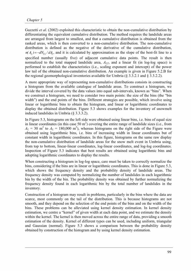
There is much to be learnt from the analysis of Figure 5.7. First, all obtained probability densities exhibit a similar trend. The probability density increases with the area of the landslide up to a maximum value, where slope failures are most abundant, then it decays along a power law. The slope of the power law tail of the distribution ranges from α+1 = 2.26 to α+1 = 2.91.

The size of the most abundant landslide exhibits a much larger variation. To facilitate the investigation of the relationships between the size of the most abundant landslide and the type of the inventory, in Figure 5.7 the different types of inventories (i.e., geomorphological, event, multiple-events, multi-temporal) are shown with different symbols. The reconnaissance map (§ 3.3.2.1) clearly underestimates the abundance of the smallest landslides. The most abundant slope failures in this inventory have an area of ~ 2.5×104 m2, six times larger than the area predicted by the detailed geomorphological inventory (~ 4×103 m2), and at least eight times larger than the area predicted by the 1997 snowmelt event inventory (~ 3×103 m2). When compared to the other inventories, the two geomorphological maps show a larger proportion of large and very large landslide areas. For the reconnaissance mapping this is evident for landslides larger than ~ 1×104 m2, and for the detailed geomorphological mapping for landslides larger than ~ 2×103 m2. This finding has several reasons. The geomorphological maps do not show small landslides, which were not visible in the single set of medium scale aerial photographs used to obtain the landslide information. In places, the geomorphological inventories show a number of coalescent landslides as a single larger landslide (or landslide area), overestimating the size of the larger slope failures. Lastly, the reconnaissance mapping is affected by cartographic inaccuracies, which also lead to overestimation of the size of the large landslides (§ 3.4, Carrara et al., 2002).

Noticeably, the multi-temporal inventory obtained for the Collazzone area is not affected by this bias, indicating the ability of a good quality multi-temporal landslide map to reliably describe the size of the landslides, at least for slope failures having AL ≥ 1.5×103 m2. This is an important result, as it provides the rationale for using information on landslide size obtained

Statistics of landslide size

108

from multi-temporal landslide maps to ascertain the probability of landslide area, vital information to determine landslide hazard (§ 7).

Further inspection of Figure 5.7 indicates that the inventories prepared following the 1997 snowmelt event and the multiple rainfall events in 2004 provide the smallest estimate for the area of the most abundant landslide (i.e., ~ 500 m2) which is in good agreement with what predicted by the general inverse Gamma probability density distribution of Malamud et al. (2004a). Also, the event, the multiple-events, and the multi-temporal inventories exhibit a power law tail in good agreement with what predicted by Malamud et al. (2004a).

Figure 5.7 – Umbria Region. Probability density of landslide areas for six different landslide

inventories. Geomorphological inventories are shown by continuous lines. Event and multiple events inventories are shown by dotted lines. The Collazzone multi-temporal inventory is shown by a dashed

line. Also shown is the general probability density of landslide areas proposed by Malamud et al. (2004a). Probability density obtained using equation 5.4.

Chapter 5

109

5.4. Discussion

Frequency-size statistics of landslides are important for the quantification of erosion processes in mountain areas. Statistics of landslide area and volume have been used to determine sediment fluxes and to the estimate denudation rates (Hovius et al., 1997, 2000; Martin et al., 2002; Lavé and Burbank, 2004; Malamud et al., 2004b). The Frequency-size statistics of landslides are also important for the quantification of landslide hazard (Malamud et al., 2004a; Guzzetti et al., 2005a). A discussion on these topics is not within the scope of this work (§ 1.2). In the following, I will concentrate on two relevant issues, namely: (i) why medium and large landslides consistently satisfy a power law (i.e., fractal) frequency-area statistics, and (ii) why small and very small landslides systematically deviate from the power law correlation. I will also investigate the differences between the frequency-area and the frequency-volume statistics observed in the available empirical data.

There is now clear evidence that medium and large size landslides consistently satisfy power law frequency-area statistics. Reasons for this behaviour remain undetermined. One potential explanation for this power law behaviour is the concept of self-organized criticality (SOC, Back et al., 1987, 1988). This concept was introduced to explain the behaviour of the “sandpile” model. In this model, there is a square grid of boxes, at each time step a particle is dropped into a randomly-selected box. When there are four particles in a box they are redistributed to the four adjacent boxes, or in the case of boxes on the boundaries of the grid, are lost. A single redistribution can lead to an “avalanche” of redistributions. The size of the “avalanche”’ is the area of boxes AB participating in the redistributions. The non-cumulative number of “avalanches” NA with area AB satisfies the power law distribution 01.

BA AN −≈ (Kadanoff et al., 1989).

Noever (1993) has associated the power law frequency-area statistics of large landslides with the “sandpile” model and the concept of self-organized criticality. However, there is a large extrapolation from the “sandpile” model to actual landslides. The available empirical data indicate that, for the medium and large landslides, the power law exponent is α+1 = 2.4 ± 0.4, considerably larger than the value of 1.0 predicted by the “sandpile” model (Malamud et al., 2004a). This is not surprising considering the simplicity of the model and the three-dimensional nature of actual landslides, and could indicate that a revision of the “rules” for the “sandpile” model is needed for a realistic analogue of actual landslides in nature. Pelletier et al. (1997) have combined a slope stability analysis with a soil-moisture analysis and found a power law distribution. The cumulative frequency-area distribution of the modelled landslides found by these authors has a scaling exponent α = 1.6. Hertgarten and Neugebauer (2000) have used a numerical model combining slope stability and mass movement and found an approximation to a power law distribution with an exponent of α+1 ~ 2.1. More recently, these authors have used a cellular-automata model with time-dependent weakening, similar to the “sandpile” model, and found a power law distribution with α+1 ~ 2.0 (Hertgarten and Neugebauer, 2000). Czirók et al. (1997) performed laboratory experiments using a micro-model of a ridge and produced landslides by spraying the ridge with water, thus simulating rainfall. These authors obtained a density distribution for the area of the micro-landslides that correlated with a power law with α+1 ~ 1.0, in good agreement with the “sandpile” model prediction, but different from what is observed in natural landslides. Although it is certainly possible to develop idealized models that reproduce the observed power law dependence of actual landslide data, there is a real question whether these models are realistic in terms of the governing physics (Turcotte et al., 2002).

Statistics of landslide size

110

Despite its clear limitations, the relatively simple “sandpile” model may provide the basis for understanding the power law statistics of large landslides (Malamud et al., 2004a; Turcotte et al., 2002). In the “sandpile” model the region over which an avalanche will spread is well defined prior to the avalanche. Similarly, the area over which a landslide will spread can be defined before the landslide is triggered. In both, there are metastable areas. As particles are added, the metastable avalanche areas grow. As mountains grow, metastable landslide areas also grow. Detailed studies of the “sandpile” model show that this growth is dominated by the coalescence of smaller metastable regions (Turcotte, 1999). Also, the coalescence cross sections lead directly to a power law distribution of metastable areas. It can be expected that a similar coalescence and growth process would be applicable to metastable landslide areas, explaining the observed power law frequency area distribution of large landslides.

There is also good evidence that landslide area obtained from reasonably complete (for statistical purposes) empirical inventories deviate from the power law correlation for small landslides. The reasons for this behaviour are also undetermined. One possibility is that the rollover scale has a geomorphological explanation (Guzzetti et al., 2002). The rollover occurs for linear scales less than about 30 meters, which is the scale on which well defined stream networks form. The incision associated with stream and river networks would be expected to play a significant role in the geometry of landslides, at least for climatically controlled slope failures. For climatically controlled landslides, water and groundwater are important issues and both relate to the size of the slope, which in turn depends on the pattern and density of the drainage network. For seismically induced landslides, the relationship is less clear. These landslides, and particularly rock falls and disrupted rock slides, occur where slopes are steeper, where the seismic shaking concentrates, and where the rock is weaker. An alternative explanation for the rollover of the data is that this scale represents a transition from failures controlled mostly by cohesion through the sliding mass to failures controlled mostly by basal friction. Deviation from the power law scaling for small landslide areas may also reflect geometrical characteristic of the landslides. Very large landslides exhibit – necessarily – a larger area to volume ratio. The same ratio for small landslides will depend on the type of landslides. Shallow soil slides have an area to volume ratio of 0.2 or lower, whereas small rock falls may exhibit a ratio close to 1.0 (i.e., a cube of rock sliding on one of the faces). This may also explain why the statistics of landslide volume do not change for small landslides. Indeed, in the statistics of landslide volume given in Figure 5.5 several different types of landslides are shown, including rock falls.

Frequency-size statistics of landslides have implications for landslide hazard and risk assessment. In § 7.3, I will use the probability density of landslide area obtained from a multi-temporal inventory to measure the magnitude of the expected slope failures; mandatory information to ascertain landslide hazard. There are other ways to use the statistics of landslide size to ascertain landslide hazards. Malamud et al. (2004a) investigated three substantially complete landslide event inventories (including the landslides triggered by rapid snow melting in Umbria in 1997, § 3.3.3.2) and proposed a general probability density distribution for landslide area. This general distribution is based on their inverse Gamma distribution (eq. 5.4), taking α+1 = 2.40, t = 1.28×103 m2, and s = -1.32×102 m2. Using their general distribution, these authors computed descriptive statistics for landslides, including the average area of a landslide in an inventory (ĀL =3.07×103 m2). Assuming the applicability of the proposed general distribution, other useful statistics can be computed. Where the total number of landslides in a (complete) inventory is known, the total landslide area (ALT =ĀL×NLT = (3.07×103 m2) × NLT), and the area of the largest expected landslide (ALmax = (1.10×103 m2) ×

Chapter 5

111

NLT0.714) can be easily determined. Further, assuming a relationship between landslide volume

and landslide area of the type VL = εAL1.50, the average landslide volume, LV , the total

landslide volume, VLT, and the maximum landslide volume, VLmax, can also be determined (Malamud et al., 2004a,b). This is important information to ascertain landslide hazard and risk (e.g., Cardinali et al., 2002; Reichenbach et al., 2005).

Based on the same general probability density distribution for landslide areas, Malamud et al. (2004a) proposed a magnitude scale, mL, for a landslide event, and defined it as the logarithm to the base 10 of the total number of landslides associated with the event (eq. 5.5). This is similar to what was proposed by Keefer (1984) and later by Rodríguez et al. (1999) who used a scale to quantify the number of landslides in earthquake-triggered landslide events: 100-1000 landslides were classified as a two, 1000-10,000 landslides a three, etc. Knowing the total number of landslides triggered by an event, the landslide magnitude of the event is determined as:

mL =log10 NLT (5.5)

Using this scale, the rapid snowmelt event that resulted in 4246 landslides in January 1997 in Umbria (§ 3.3.3.2) has a landslide magnitude mL = 3.63. This compares with a landslide magnitude mL = 2.80 for the prolonged rainfall periods that triggered 628 landslides in Umbria in 2004.

Malamud et al. (2004a,b) further combined the landslide volume statistics obtained from their general distribution, with an empirical correlation obtained by Keffer (1994) between the total volume of landslides, VLT, triggered by an earthquake and the magnitude ME of the earthquake, and obtained an approximate relation between the earthquake magnitude ME and the magnitude of the landslide event, mL, triggered by the earthquake. This relation is

mL =1.29ME – 5.65 (5.6)

This is important information for the determination of the hazard posed by earthquake induced landslides. Unfortunately, no similar correlations are available for landslides triggered by rainfall or snowmelt, largely because no established measure exists for the magnitude of these meteorological events.

5.5. Summary of achieved results

In this chapter, I have:

(a) Shown how to obtain reliable statistics of landslide area and volume from landslide inventory maps or landslide catalogues.

(b) Demonstrated how statistical information on landslide area can be used to evaluate the completeness of a landslide inventory, contributing to establish the quality of the inventory.

(c) Shown how statistics of landslide area and volume can prove useful to determine landslide hazard and the associated risk.

This responds to Question # 4 and contributes to respond to Question # 2 given in the Introduction (§ 1.2).