05-CH-V Environmental impact assesment pg 94-122 · 94 CHAPTER - V ENVIRONMENTAL IMPACT ASSESSMENT 1. The impacts on various environmental components are expected due to the construction

94

CHAPTER - V

ENVIRONMENTAL IMPACT ASSESSMENT

1. The impacts on various environmental components are expected due to the

construction and operational activities of the proposed coal fired thermal power station. The overall environmental impact is broadly divided into impacts during construction phase and operation phase. Both quantitative and qualitative impacts are assessed for various environmental components. The details of impact identification, prediction and assessment are given in this chapter.

CONSTRUCTION PHASE

2. During construction, activities like drilling, concreting, piling and installation of piping racks will be performed. Temporarily, some of the environmental parameters may get disturbed during the construction phase. The impact of each of these parameters is discussed below:

AIR IMPACT

3. The major source of air pollution during the construction period is from the movement of vehicles for construction activity. The emissions are from the stationary sources like generator sets during emergency service only, and air borne dust emissions from cutting and filling of soil and vehicular movements. The exhaust emission along with the dust emissions resulting from vehicles operating at site will also add to air impact. Dust suppression by spraying of water will reduce these impacts considerably.

4. The emission from vehicles will depend on the type and capacity of the

vehicles used. The impact due to additional vehicles plying during the construction period is of temporary nature and their impact on air quality will not be significant.

NOISE IMPACT

5. The major sources of the noise pollution due to construction activity is from the earth moving, levelling and compacting, trucks for transportation of construction materials, concrete mixers, asphalt mixing and laying equipment all add to the general noise level.

6. The noise generated from all construction activities will be restricted to daytime working hours. Generally the noise will be limited very much within the site boundary except noise of piling work for pile foundation, the trucks entering and leaving the site. Geotechnical investigation would be taken into consideration in such a way that may not encounter any solid rock to be blasted. Hence, noise impact from blasting operation is expected to be minimal.

7. Further the noise impact during construction will be temporary in nature. The noise level will drop down to the acceptable level, once construction period will be over.

95

WATER POLLUTION IMPACT

8. During construction, the runoff from the construction site is a source of water pollution. Such pollution may persist entirely during the initial phase of construction when site grading and excavation for foundation and back filling would be in progress. During this stage the rainwater runoff would carry more soil/silt than normal and this would cause silting problem in the receiving water bodies.

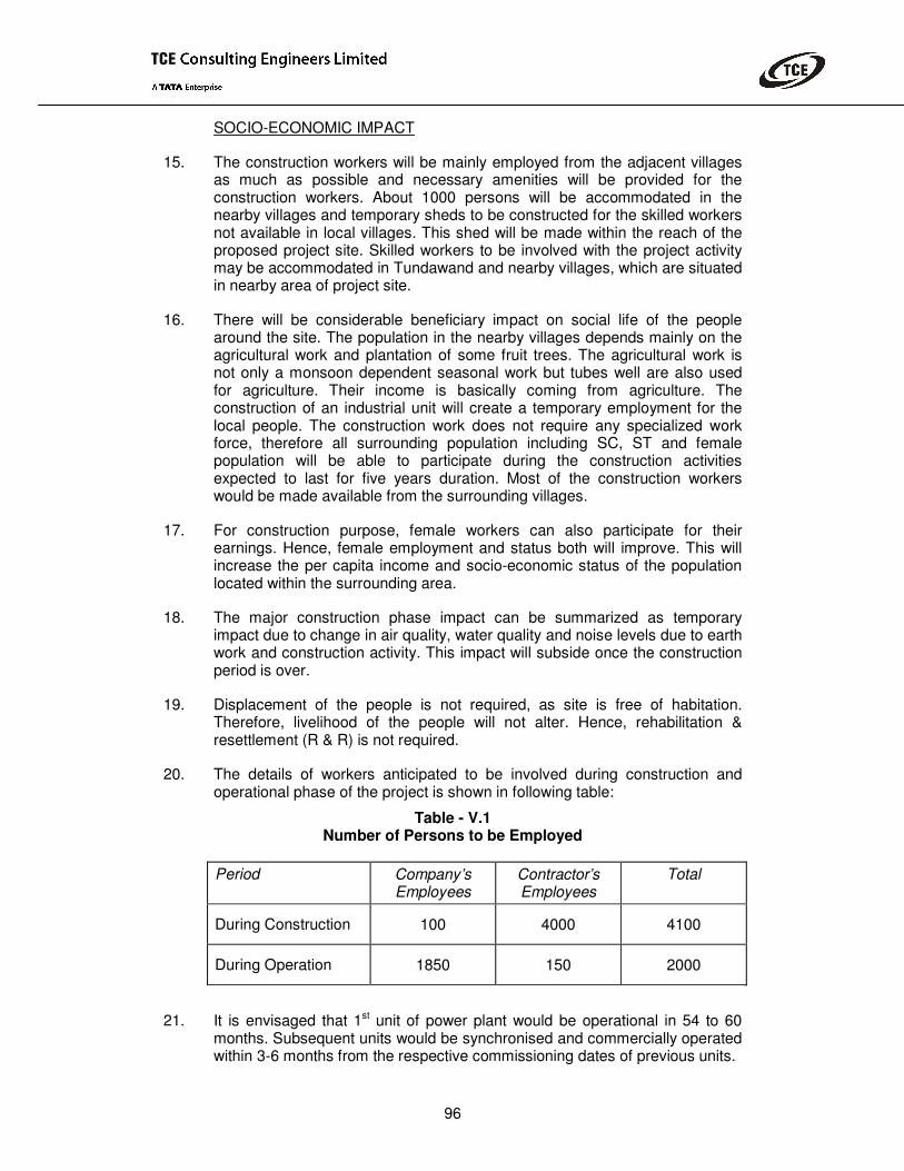
9. Construction management would include the following steps to ensure that such problem are kept to absolute minimum:

a) Undertake site grading and excavation for foundation and back filling during dry season.

b) If called for, runoff water from unstabilised fill area, should be channelled and routed to the receiving water body through a settling basin.

10. Prior to construction a peripheral drain and settling pond would be provided to collect the rain runoff. This will prevent the loose soil getting washed away from the site.

11. The other source of water pollution is expected from the sanitary waste coming from the temporary accommodation of the construction workers if envisaged. Approximately 1000 temporary contractor workers are expected to be involved in construction phase. However, most of the construction workers will be made available from the near by villages and no separate migration of workers is envisaged for this project. The facilities presently available with the villages will continue to be used during construction activities and no sanitation problem is expected during construction period. However, on site during working hours additional sanitation will be handled by septic tank/pit if required, the arrangement will be made available during the construction phase of the project.

12. The construction activity for this project is temporary in nature and not likely to have significant impact on the quality of ground water.

ECOLOGICAL IMPACT

13. The proposed mega power project is planned on plain/ barren & muddy land. Land will be acquired for the project. There is no fauna habitat recorded in the proposed project area. The site is neither an ecologically sensitive nor a place of ecological importance. There would be minimum requirement of tree felling for the construction of project. Therefore, significant ecological impact is not envisaged during construction phase of the proposed mega power plant.

14. Construction of intake and outfall structure will be done in such a manner, which will have minimum impact on existing marine and terrestrial ecology. Recommendation of CWPRS/NIO study (This study shall be completed before starting the construction work at site) for design of structure shall be strictly adhered to avoid any ecological disturbance. Mangroves or any other tree species are not reported along the tentative route of intake and outfall structure. Adoption of good construction management practices will minimize the impacts on surrounding ecology to the bare minimal level.

96

SOCIO-ECONOMIC IMPACT

15. The construction workers will be mainly employed from the adjacent villages as much as possible and necessary amenities will be provided for the construction workers. About 1000 persons will be accommodated in the nearby villages and temporary sheds to be constructed for the skilled workers not available in local villages. This shed will be made within the reach of the proposed project site. Skilled workers to be involved with the project activity may be accommodated in Tundawand and nearby villages, which are situated in nearby area of project site.

16. There will be considerable beneficiary impact on social life of the people around the site. The population in the nearby villages depends mainly on the agricultural work and plantation of some fruit trees. The agricultural work is not only a monsoon dependent seasonal work but tubes well are also used for agriculture. Their income is basically coming from agriculture. The construction of an industrial unit will create a temporary employment for the local people. The construction work does not require any specialized work force, therefore all surrounding population including SC, ST and female population will be able to participate during the construction activities expected to last for five years duration. Most of the construction workers would be made available from the surrounding villages.

17. For construction purpose, female workers can also participate for their earnings. Hence, female employment and status both will improve. This will increase the per capita income and socio-economic status of the population located within the surrounding area.

18. The major construction phase impact can be summarized as temporary impact due to change in air quality, water quality and noise levels due to earth work and construction activity. This impact will subside once the construction period is over.

19. Displacement of the people is not required, as site is free of habitation. Therefore, livelihood of the people will not alter. Hence, rehabilitation & resettlement (R & R) is not required.

20. The details of workers anticipated to be involved during construction and operational phase of the project is shown in following table:

Table - V.1 Number of Persons to be Employed

Period Company’s

Employees Contractor’s Employees

Total

During Construction 100 4000 4100

During Operation 1850 150 2000

21. It is envisaged that 1st unit of power plant would be operational in 54 to 60 months. Subsequent units would be synchronised and commercially operated within 3-6 months from the respective commissioning dates of previous units.

97

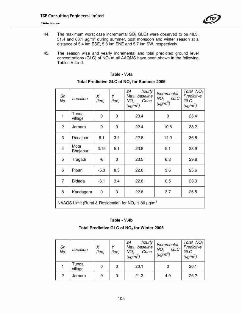
OPERATION PHASE

AIR QUALITY

22. The proposed coal based thermal power station will have pollutant emission in form of SO2, NOx, and SPM from flue gas of the stacks. The imported coal to be used has upto 1.0% sulphur content that will contribute for SO2 emission. The particulate emission from stack is 100 mg/ N cu.m of flue gas. Air pollution dispersion modeling has been carried out for SO2, ,NOx and SPM. These emissions will disperse in the atmosphere depending on the atmospheric conditions. The atmospheric conditions that affect the dispersion of pollutants are:

• Wind direction and wind speed.

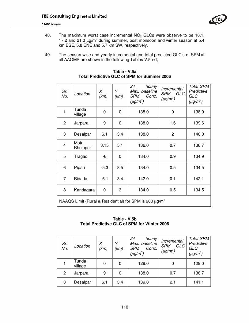
• Ambient temperature.

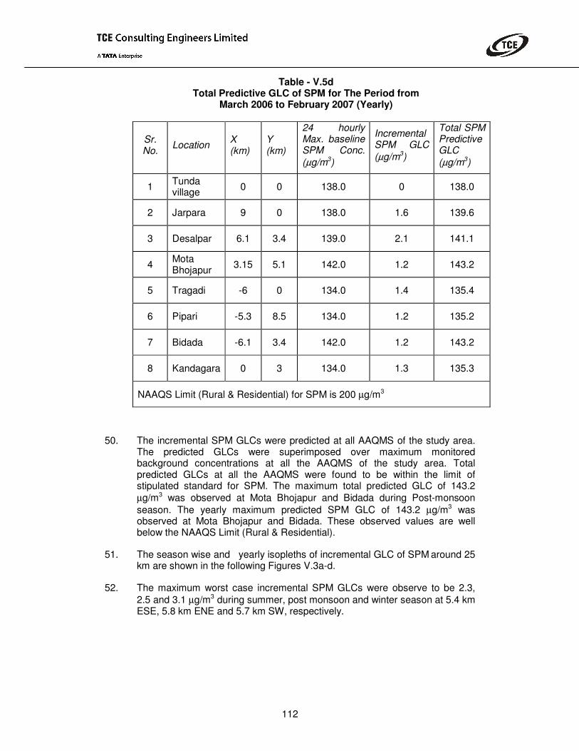
• Atmospheric stability: Atmospheric stability depends on the wind speed and solar radiation intensity or cloud cover. During night time the cloud cover, wind speed are considered for the stability calculation. More unstable condition will lead to better dispersion and stable condition will have less dispersion.

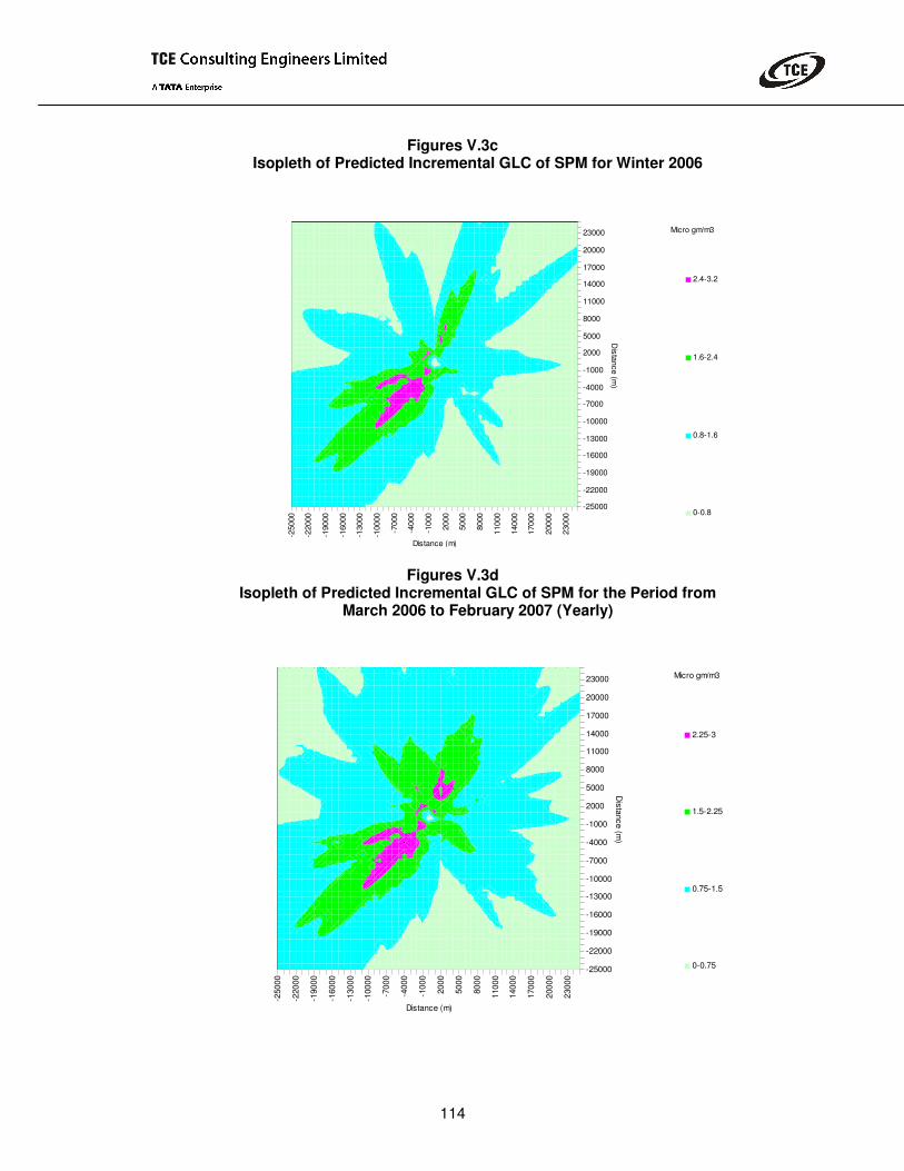
• Mixing height: Mixing height is the region between the bottom of the inversion layer and the ground. The inversion layer is a dynamic region, which changes depending on the atmospheric condition. The mixing height can be calculated based on the vertical temperature profile of the atmosphere. Mixing height for Delhi, Bombay and Calcutta and major cities in all state are published by Central Pollution Control Board. Indian Meteorological Department (IMD) is regularly monitoring the vertical temperature profiles at 35 locations. This data can be used for calculating the mixing height at any specific location. However, site-specific mixing height data is not available. Mixing height data available for morning and evening time at nearest observatory at Ahmedabad has been used for present study. The recorded mixing height data for summer, post-monsoon and winter season are shown in Appendix –25a-c.

INPUTS USED FOR DISPERSION MODELLING

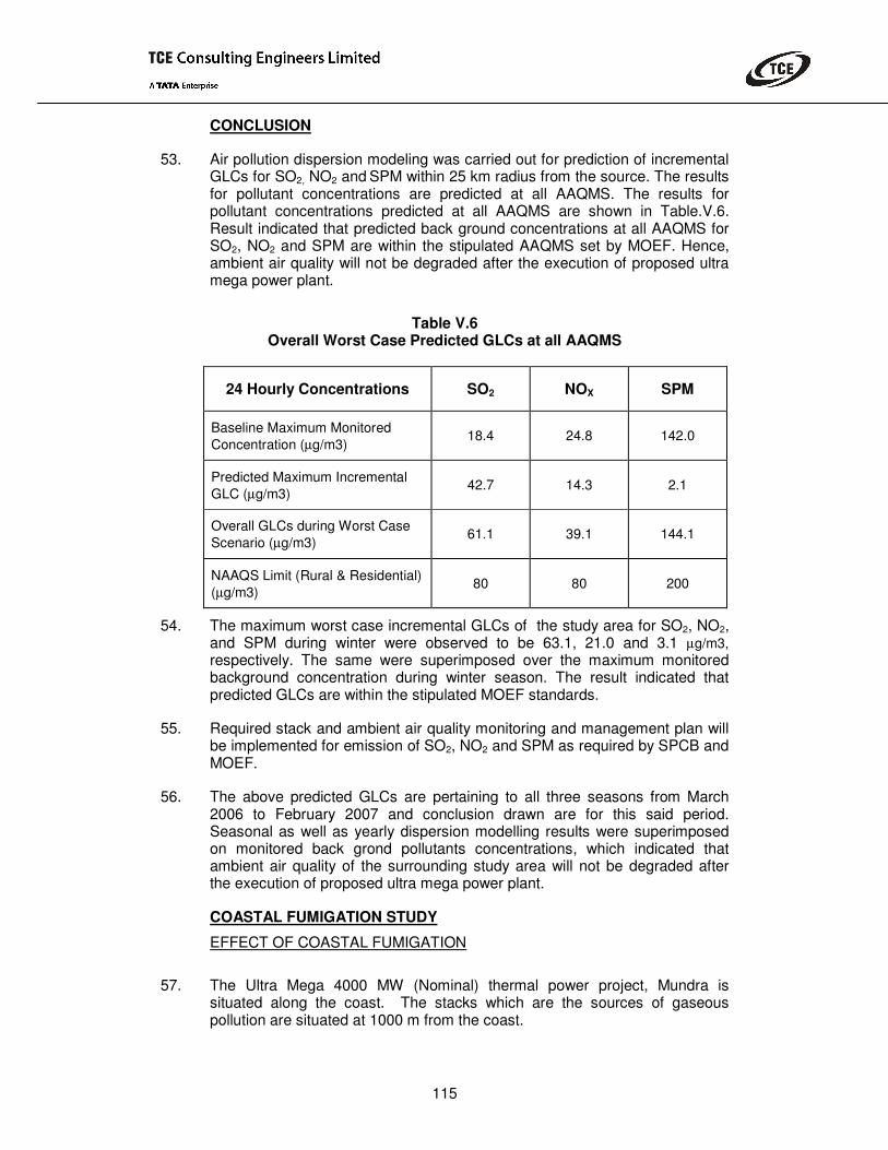
Emission Data

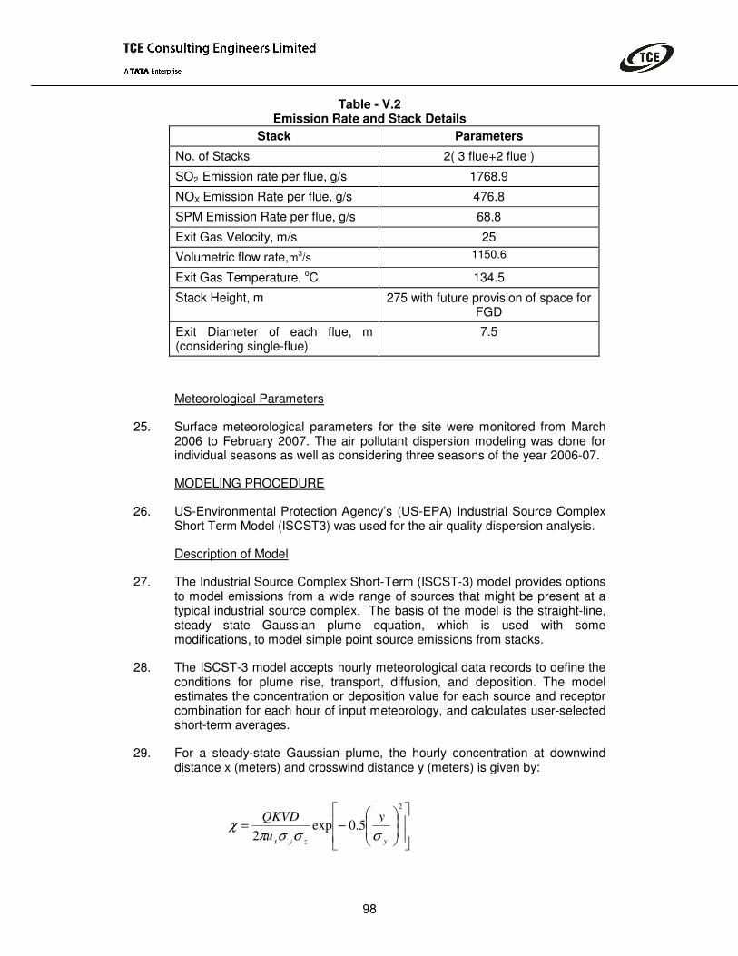
23. The important pollutant of the proposed 4000 MW (Nominal) coal based thermal power station is mainly SO2, oxide of nitrogen (NOX) as NO2 , and SPM. Therefore, prediction of GLCs are considered for SO2 , NOX and SPM emission. The emission from the stack is considered to be constantly distributed throughout the day for the dispersion analysis. Two multiflue stack(one with 3 flues and the second one with 2 flues, each flue of 7.5m inside diameter) .These stacks are located at a inter stack distance of 250m each in a straight line at the project site.

24. The emission rate and stack details for each stack considered for air pollution dispersion analysis is given in Table V.2.

98

Table - V.2 Emission Rate and Stack Details

Stack Parameters

No. of Stacks 2( 3 flue+2 flue )

SO2 Emission rate per flue, g/s 1768.9

NOX Emission Rate per flue, g/s 476.8

SPM Emission Rate per flue, g/s 68.8

Exit Gas Velocity, m/s 25

Volumetric flow rate,m3/s 1150.6

Exit Gas Temperature, oC 134.5

Stack Height, m 275 with future provision of space for FGD

Exit Diameter of each flue, m (considering single-flue)

7.5

Meteorological Parameters

25. Surface meteorological parameters for the site were monitored from March 2006 to February 2007. The air pollutant dispersion modeling was done for individual seasons as well as considering three seasons of the year 2006-07.

MODELING PROCEDURE

26. US-Environmental Protection Agency’s (US-EPA) Industrial Source Complex Short Term Model (ISCST3) was used for the air quality dispersion analysis.

Description of Model

27. The Industrial Source Complex Short-Term (ISCST-3) model provides options to model emissions from a wide range of sources that might be present at a typical industrial source complex. The basis of the model is the straight-line, steady state Gaussian plume equation, which is used with some modifications, to model simple point source emissions from stacks.

28. The ISCST-3 model accepts hourly meteorological data records to define the conditions for plume rise, transport, diffusion, and deposition. The model estimates the concentration or deposition value for each source and receptor combination for each hour of input meteorology, and calculates user-selected short-term averages.

29. For a steady-state Gaussian plume, the hourly concentration at downwind distance x (meters) and crosswind distance y (meters) is given by:

��

�

�

��

�

�

��

�

�

�−=

2

5.0exp2

yzys

yu

QKVDσσσπ

χ

99

where, Q = pollutant emission rate (mass per unit time) K = a scaling coefficient to convert calculated concentrations to

desired units (default value of 1 x 106 for Q in g/s and concentration in µg/m3)

V = vertical term D = decay term

σy,σz = standard deviation of lateral and vertical concentration distribution (m)

us = mean wind speed (m/s) at release height.

30. The Vertical Term includes the effects of source elevation, receptor elevation, plume rise, limited mixing in the vertical, and the gravitational settling and dry deposition of particulate (with diameters greater than about 0.1 microns).

31. The ISC model uses either a polar or a Cartesian receptor network as specified by the user. In the Cartesian coordinate system, the X-axis is positive to the east of the user-specified origin and the Y-axis is positive to the north.

32. The wind power law is used to adjust the observed wind speed, uref, from a reference measurement height, zref, to the stack or release height, hs using power law equation.

33. The plume height is used in the calculation of the Vertical Term”V”. This is the effective release height of the effluent. This is made up of physical stack height and plume rise due to buoyancy or momentum. In this case the plume rise will be controlled by buoyancy.

34. Appropriate plume rise formulations have been used in this model. The effective plume rise for various weather conditions and wind speed are used.

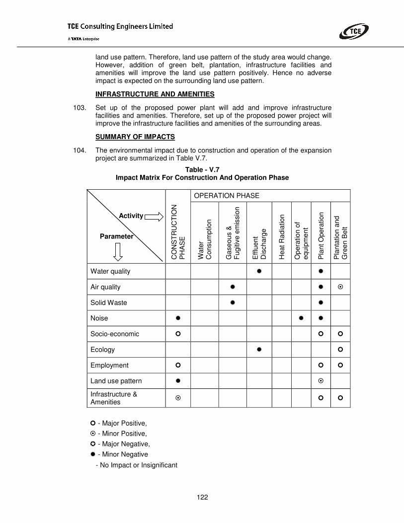
35. The method of Pasquill (1976) is used to account for the initial dispersion of plumes caused by turbulent motion of the plume and turbulent entrainment of ambient air.

36. The infinite series term in the above Equation accounts for the effects of the restriction on vertical plume growth at the top of the mixing layer. The Equation assumes that the mixing height in rural and urban areas is known for all stability categories. The ISCST models currently assume unlimited vertical mixing under stable conditions, and therefore delete the infinite series term in the Equation for the E and F stability categories.

37. Pollutants traveling down wind will be reflected at the ground. The elevated inversion layer (mixing height) will also reflect the pollutant. At long downwind distances the plume concentration will be fully mixed vertically. This effect has also been built up in the program (model) formulation.

INPUTS TO ISCST3 MODEL

38. Pollution dispersion calculation was done only for NOX, SO2 and SPM emission by using ISCST3 model. Emission of fly ash as particulate matter is

100

controlled due to installation of electro static precipitator (ESP) as pollution control equipment. The fuel is coal, which contains maximum 1.0% sulfur. Therefore, proposed mega power plant will have contribution of SO2 and NOX

emission. The area has been divided into 500m grid and the ground level concentration of the pollutant at each grid point was calculated. Total area for calculation of incremental GLCs has been considered for 25 km radius from the source.

39. The plume spread parameters σy and σz in a double Gaussian dispersion model depend upon the sampling or averaging time. Consequently, the concentration measured at a given location also depends upon the sampling time. The parameters used here pertain to a sampling time of 10 minutes. We are using 1 hour average data of wind speed and wind direction and use of this will give 1 hour average concentration value.

40. The σy value has to be corrected for the averaging time factor. The correction factor is given by:

X 1h, 10min = (10/60) 0.12 = 0.807 = (1/1.24)

That is σy from Pasquill graphs/Briggs formulation has to be multiplied by 1.24 or the concentration has to be reduced by a factor of 0.807. (Air Pollution Meteorology by V. V. Shirvaikar and V. J. Daoo – BARC/2002/E/013 – page 91)

MODELLING RESULTS

41. The season wise and yearly incremental and total predicted ground level concentrations (GLC) of SO2 at all AAQMS have been shown in the following Tables V.3a-d;

Table - V.3a Total Predictive GLCs of SO2 for Summer 2006

Sr. No. Location X

(km) Y (km)

24 hourly Max. baseline SO2 Conc. (µg/m3)

Incremental SO2 GLC (µg/m3)

Total SO2 Predictive

GLC (µg/m3)

1 Tunda village 0 0 16.2 0 16.2

2 Jarpara 9 0 15.4 32.2 47.6

3 Desalpar 6.1 3.4 15.4 41.7 57.1

4 Mota Bhojapur 3.15 5.1 18.4 15.1 33.5

5 Tragadi -6 0 14.2 18.8 33.0

6 Pipari -5.3 8.5 13.0 10.7 23.7

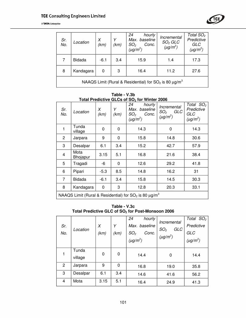
101

Sr. No. Location X

(km) Y (km)



Total SO2 Predictive

GLC (µg/m3)

7 Bidada -6.1 3.4 15.9 1.4 17.3

8 Kandagara 0 3 16.4 11.2 27.6

NAAQS Limit (Rural & Residential) for SO2 is 80 µg/m3

Table - V.3b

Total Predictive GLCs of SO2 for Winter 2006

Sr. No. Location X

(km) Y (km)



Total SO2 Predictive GLC (µg/m3)

1 Tunda village 0 0 14.3 0 14.3

2 Jarpara 9 0 15.8 14.8 30.6

3 Desalpar 6.1 3.4 15.2 42.7 57.9

4 Mota Bhojapur 3.15 5.1 16.8 21.6 38.4

5 Tragadi -6 0 12.6 29.2 41.8

6 Pipari -5.3 8.5 14.8 16.2 31

7 Bidada -6.1 3.4 15.8 14.5 30.3

8 Kandagara 0 3 12.8 20.3 33.1


Table - V.3c Total Predictive GLC of SO2 for Post-Monsoon 2006

Sr.

No. Location

X

(km)

Y

(km)

24 hourly

Max. baseline

SO2 Conc.

(µg/m3)

Incremental

SO2 GLC

(µg/m3)

Total SO2

Predictive

GLC

(µg/m3)

1 Tunda

village 0 0 14.4 0 14.4

2 Jarpara 9 0 16.8 19.0 35.8

3 Desalpar 6.1 3.4 14.6 41.6 56.2

4 Mota 3.15 5.1 16.4 24.9 41.3

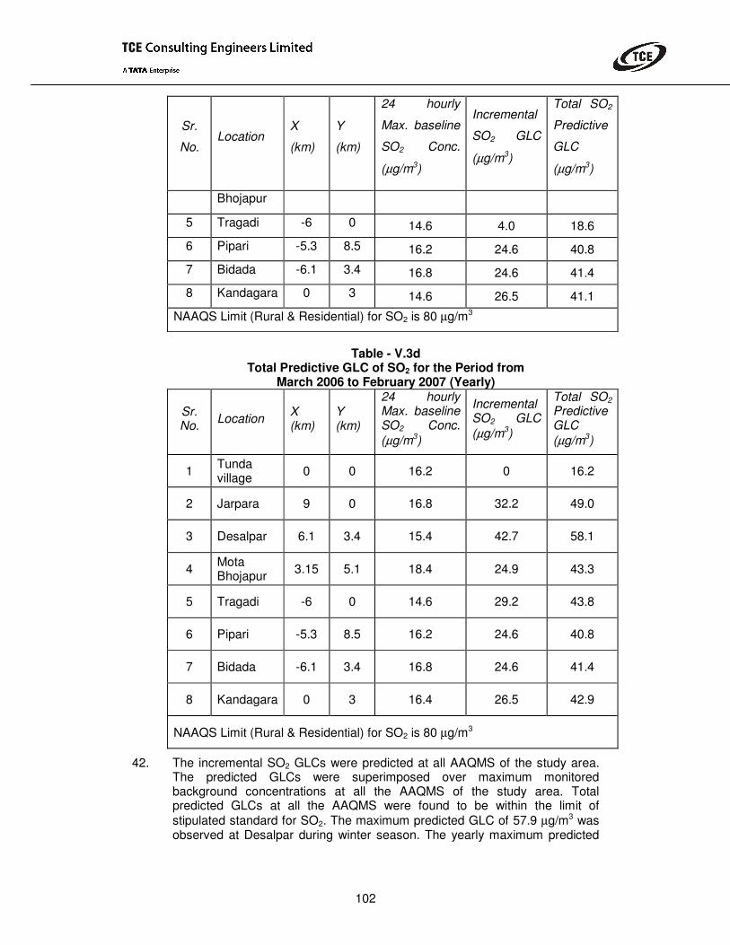
102

Sr.

No. Location

X

(km)

Y

(km)

24 hourly

Max. baseline

SO2 Conc.

(µg/m3)

Incremental

SO2 GLC

(µg/m3)

Total SO2

Predictive

GLC

(µg/m3)

Bhojapur

5 Tragadi -6 0 14.6 4.0 18.6

6 Pipari -5.3 8.5 16.2 24.6 40.8

7 Bidada -6.1 3.4 16.8 24.6 41.4

8 Kandagara 0 3 14.6 26.5 41.1


Table - V.3d

Total Predictive GLC of SO2 for the Period from March 2006 to February 2007 (Yearly)

Sr. No. Location X

(km) Y (km)



Total SO2 Predictive GLC (µg/m3)

1 Tunda village 0 0 16.2 0 16.2

2 Jarpara 9 0 16.8 32.2 49.0

3 Desalpar 6.1 3.4 15.4 42.7 58.1

4 Mota Bhojapur 3.15 5.1 18.4 24.9 43.3

5 Tragadi -6 0 14.6 29.2 43.8

6 Pipari -5.3 8.5 16.2 24.6 40.8

7 Bidada -6.1 3.4 16.8 24.6 41.4

8 Kandagara 0 3 16.4 26.5 42.9


42. The incremental SO2 GLCs were predicted at all AAQMS of the study area. The predicted GLCs were superimposed over maximum monitored background concentrations at all the AAQMS of the study area. Total predicted GLCs at all the AAQMS were found to be within the limit of stipulated standard for SO2. The maximum predicted GLC of 57.9 µg/m3 was observed at Desalpar during winter season. The yearly maximum predicted

103

-250

00

-220

00

-190

00

-160

00

-130

00

-100

00

-700

0

-400

0

-100

0

2000

5000

8000

1100

0

1400

0

1700

0

2000

0

2300

0

-25000

-22000

-19000

-16000

-13000

-10000

-7000

-4000

-1000

2000

5000

8000

11000

14000

17000

20000

23000 Micro gm/m3

Distance (m)

Distance (m

)

37.5-50

25-37.5

12.5-25

0-12.5

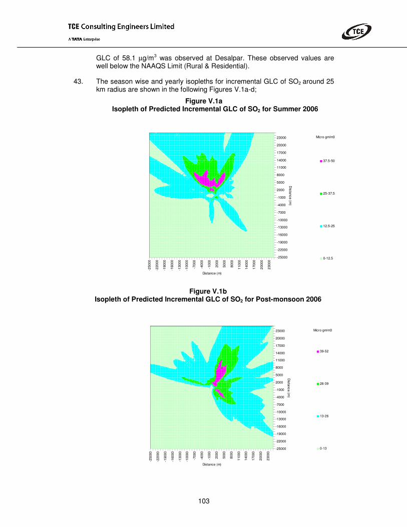
GLC of 58.1 µg/m3 was observed at Desalpar. These observed values are well below the NAAQS Limit (Rural & Residential).

43. The season wise and yearly isopleths for incremental GLC of SO2 around 25 km radius are shown in the following Figures V.1a-d;

Figure V.1a Isopleth of Predicted Incremental GLC of SO2 for Summer 2006

Figure V.1b Isopleth of Predicted Incremental GLC of SO2 for Post-monsoon 2006

-250

00

-220

00

-190

00

-160

00

-130

00

-100

00

-700

0

-400

0

-100

0

2000

5000

8000

1100

0

1400

0

1700

0

2000

0

2300

0

-25000

-22000

-19000

-16000

-13000

-10000

-7000

-4000

-1000

2000

5000

8000

11000

14000

17000

20000

23000 Micro gm/m3

Distance (m)

Distance (m

)

39-52

26-39

13-26

0-13

104

-250

00

-220

00

-190

00

-160

00

-130

00

-100

00

-700

0

-400

0

-100

0

2000

5000

8000

1100

0

1400

0

1700

0

2000

0

2300

0

-25000

-22000

-19000

-16000

-13000

-10000

-7000

-4000

-1000

2000

5000

8000

11000

14000

17000

20000

23000 Micro gm/m3

Distance (m)

Distance (m

)48-64

32-48

16-32

0-16

-250

00

-220

00

-190

00

-160

00

-130

00

-100

00

-700

0

-400

0

-100

0

2000

5000

8000

1100

0

1400

0

1700

0

2000

0

2300

0

-25000

-22000

-19000

-16000

-13000

-10000

-7000

-4000

-1000

2000

5000

8000

11000

14000

17000

20000

23000 Micro gm/m3

Distance (m)

Distance (m

)

48-64

32-48

16-32

0-16

Figure V.1c

Isopleth of Predicted Incremental GLC of SO2 for Winter 2006

Figure V.1d Isopleth of Predicted Incremental GLC of SO2 for the Period from

March 2006 to February 2007(Yearly)

105

44. The maximum worst case incremental SO2 GLCs were observed to be 48.3, 51.4 and 63.1 µg/m3 during summer, post monsoon and winter season at a distance of 5.4 km ESE, 5.8 km ENE and 5.7 km SW, respectively.

45. The season wise and yearly incremental and total predicted ground level concentrations (GLC) of NO2 at all AAQMS have been shown in the following Tables V.4a-d.

Table - V.4a

Total Predictive GLC of NO2 for Summer 2006

Sr. No. Location X

(km) Y (km)

24 hourly Max. baseline NO2 Conc. (µg/m3)

Incremental NO2 GLC (µg/m3)

Total NO2 Predictive GLC (µg/m3)

1 Tunda village 0 0 23.4 0 23.4

2 Jarpara 9 0 22.4 10.8 33.2

3 Desalpar 6.1 3.4 22.8 14.0 36.8

4 Mota Bhojapur 3.15 5.1 23.8 5.1 28.9

5 Tragadi -6 0 23.5 6.3 29.8

6 Pipari -5.3 8.5 22.0 3.6 25.6

7 Bidada -6.1 3.4 22.8 0.5 23.3

8 Kandagara 0 3 22.8 3.7 26.5

NAAQS Limit (Rural & Residential) for NO2 is 80 µg/m3

Table - V.4b

Total Predictive GLC of NO2 for Winter 2006

Sr. No. Location X

(km) Y (km)




1 Tunda village 0 0 20.1 0 20.1

2 Jarpara 9 0 21.3 4.9 26.2

106

Sr. No. Location X

(km) Y (km)




3 Desalpar 6.1 3.4 21.1 14.3 35.4

4 Mota Bhojapur 3.15 5.1 21.2 7.2 28.4

5 Tragadi -6 0 16.4 9.8 26.2

6 Pipari -5.3 8.5 17.9 5.4 23.3

7 Bidada -6.1 3.4 20.8 4.9 25.7

8 Kandagara 0 3 17.6 6.8 24.4


Table - V.4c

Total Predictive GLC of NO2 for Post-Monsoon 2006

Sr. No. Location X

(km) Y (km)




1 Tunda village 0 0 21.6 0 21.6

2 Jarpara 9 0 22.8 6.3 29.1

3 Desalpar 6.1 3.4 22.6 13.9 36.5

4 Mota Bhojapur 3.15 5.1 24.8 8.3 33.1

5 Tragadi -6 0 20.4 1.3 21.7

6 Pipari -5.3 8.5 21.2 8.2 29.4

7 Bidada -6.1 3.4 22.1 8.2 30.3

8 Kandagara 0 3 21.6 8.8 30.4


107

Table - V.4d

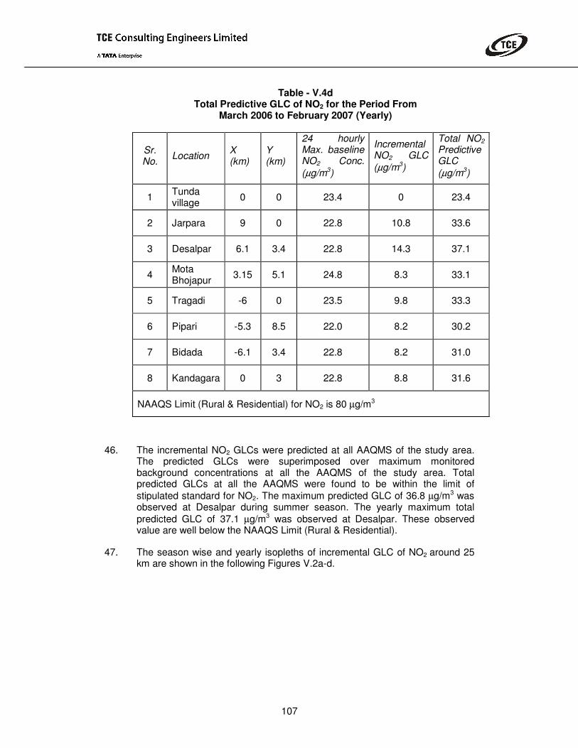
Total Predictive GLC of NO2 for the Period From March 2006 to February 2007 (Yearly)

Sr. No. Location X

(km) Y (km)




1 Tunda village 0 0 23.4 0 23.4

2 Jarpara 9 0 22.8 10.8 33.6

3 Desalpar 6.1 3.4 22.8 14.3 37.1

4 Mota Bhojapur 3.15 5.1 24.8 8.3 33.1

5 Tragadi -6 0 23.5 9.8 33.3

6 Pipari -5.3 8.5 22.0 8.2 30.2

7 Bidada -6.1 3.4 22.8 8.2 31.0

8 Kandagara 0 3 22.8 8.8 31.6


46. The incremental NO2 GLCs were predicted at all AAQMS of the study area. The predicted GLCs were superimposed over maximum monitored background concentrations at all the AAQMS of the study area. Total predicted GLCs at all the AAQMS were found to be within the limit of stipulated standard for NO2. The maximum predicted GLC of 36.8 µg/m3 was observed at Desalpar during summer season. The yearly maximum total predicted GLC of 37.1 µg/m3 was observed at Desalpar. These observed value are well below the NAAQS Limit (Rural & Residential).

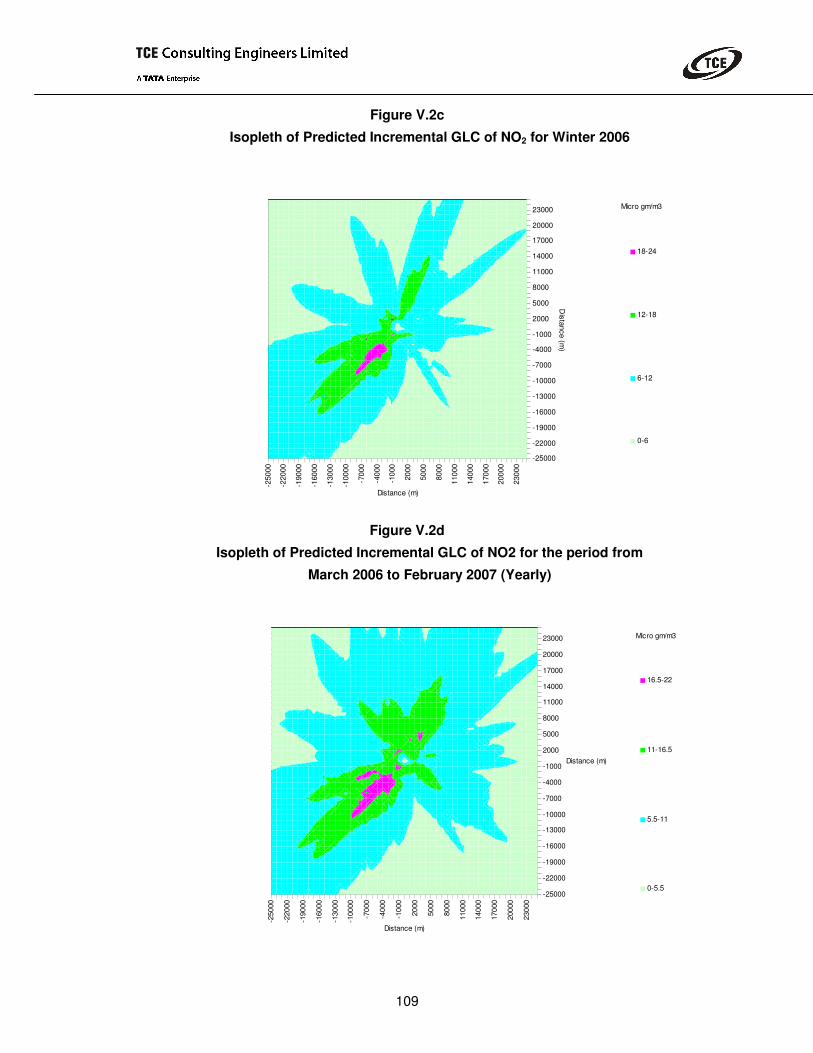
47. The season wise and yearly isopleths of incremental GLC of NO2 around 25 km are shown in the following Figures V.2a-d.

108

-250

00

-220

00

-190

00

-160

00

-130

00

-100

00

-700

0

-400

0

-100

0

2000

5000

8000

1100

0

1400

0

1700

0

2000

0

2300

0

-25000

-22000

-19000

-16000

-13000

-10000

-7000

-4000

-1000

2000

5000

8000

11000

14000

17000

20000

23000 Micro gm/m3

Distance (m)

Distance (m)

13.5-18

9-13.5

4.5-9

0-4.5

Figure V.2a Isopleth of Predicted Incremental GLC of NO2 for Summer 2006

-250

00

-220

00

-190

00

-160

00

-130

00

-100

00

-700

0

-400

0

-100

0

2000

5000

8000

1100

0

1400

0

1700

0

2000

0

2300

0

-25000

-22000

-19000

-16000

-13000

-10000

-7000

-4000

-1000

2000

5000

8000

11000

14000

17000

20000

23000Micro gm/m3

Distance (m)

Distance (m

)13.5-18

9-13.5

4.5-9

0-4.5

Figure V.2b

Isopleth of Predicted Incremental GLC of NO2 for Post-monsoon 2006

109

-250

00

-220

00

-190

00

-160

00

-130

00

-100

00

-700

0

-400

0

-100

0

2000

5000

8000

1100

0

1400

0

1700

0

2000

0

2300

0

-25000

-22000

-19000

-16000

-13000

-10000

-7000

-4000

-1000

2000

5000

8000

11000

14000

17000

20000

23000 Micro gm/m3

Distance (m)

Distance (m)

16.5-22

11-16.5

5.5-11

0-5.5

Figure V.2c

Isopleth of Predicted Incremental GLC of NO2 for Winter 2006

-250

00

-220

00

-190

00

-160

00

-130

00

-100

00

-700

0

-400

0

-100

0

2000

5000

8000

1100

0

1400

0

1700

0

2000

0

2300

0

-25000

-22000

-19000

-16000

-13000

-10000

-7000

-4000

-1000

2000

5000

8000

11000

14000

17000

20000

23000 Micro gm/m3

Distance (m)

Distance (m

)18-24

12-18

6-12

0-6

Figure V.2d

Isopleth of Predicted Incremental GLC of NO2 for the period from

March 2006 to February 2007 (Yearly)

110

48. The maximum worst case incremental NO2 GLCs were observe to be 16.1, 17.2 and 21.0 µg/m3 during summer, post monsoon and winter season at 5.4 km ESE, 5.8 ENE and 5.7 km SW, respectively.

49. The season wise and yearly incremental and total predicted GLC’s of SPM at all AAQMS are shown in the following Tables V.5a-d;

Table - V.5a

Total Predictive GLC of SPM for Summer 2006

Sr. No. Location X

(km) Y (km)

24 hourly Max. baseline SPM Conc. (µg/m3)

Incremental SPM GLC (µg/m3)

Total SPM Predictive GLC (µg/m3)

1 Tunda village 0 0 138.0 0 138.0

2 Jarpara 9 0 138.0 1.6 139.6

3 Desalpar 6.1 3.4 138.0 2 140.0

4 Mota Bhojapur 3.15 5.1 136.0 0.7 136.7

5 Tragadi -6 0 134.0 0.9 134.9

6 Pipari -5.3 8.5 134.0 0.5 134.5

7 Bidada -6.1 3.4 142.0 0.1 142.1

8 Kandagara 0 3 134.0 0.5 134.5

NAAQS Limit (Rural & Residential) for SPM is 200 µg/m3

Table - V.5b Total Predictive GLC of SPM for Winter 2006

Sr. No. Location X

(km) Y (km)




1 Tunda village 0 0 129.0 0 129.0

2 Jarpara 9 0 138.0 0.7 138.7

3 Desalpar 6.1 3.4 139.0 2.1 141.1

111

Sr. No. Location X

(km) Y (km)




4 Mota Bhojapur 3.15 5.1 137.0 1.1 138.1

5 Tragadi -6 0 124.0 1.5 125.5

6 Pipari -5.3 8.5 123.0 0.8 123.8

7 Bidada -6.1 3.4 136.0 0.7 136.7

8 Kandagara 0 3 128.0 1.0 129.0


Table - V.5c Total Predictive GLC of SPM for Post-Monsoon 2006

Sr. No. Location X

(km) Y (km)




1 Tunda village 0 0 130.0 0 130.0

2 Jarpara 9 0 138.0 0.9 138.9

3 Desalpar 6.1 3.4 138.0 2.0 140.0

4 Mota Bhojapur 3.15 5.1 142.0 1.2 143.2

5 Tragadi -6 0 124.0 0.2 124.2

6 Pipari -5.3 8.5 116.0 1.2 117.2

7 Bidada -6.1 3.4 142.0 1.2 143.2

8 Kandagara 0 3 128.0 1.3 129.3


112

Table - V.5d Total Predictive GLC of SPM for The Period from


Sr. No. Location X

(km) Y (km)




1 Tunda village 0 0 138.0 0 138.0

2 Jarpara 9 0 138.0 1.6 139.6

3 Desalpar 6.1 3.4 139.0 2.1 141.1

4 Mota Bhojapur 3.15 5.1 142.0 1.2 143.2

5 Tragadi -6 0 134.0 1.4 135.4

6 Pipari -5.3 8.5 134.0 1.2 135.2

7 Bidada -6.1 3.4 142.0 1.2 143.2

8 Kandagara 0 3 134.0 1.3 135.3


50. The incremental SPM GLCs were predicted at all AAQMS of the study area. The predicted GLCs were superimposed over maximum monitored background concentrations at all the AAQMS of the study area. Total predicted GLCs at all the AAQMS were found to be within the limit of stipulated standard for SPM. The maximum total predicted GLC of 143.2 µg/m3 was observed at Mota Bhojapur and Bidada during Post-monsoon season. The yearly maximum predicted SPM GLC of 143.2 µg/m3 was observed at Mota Bhojapur and Bidada. These observed values are well below the NAAQS Limit (Rural & Residential).

51. The season wise and yearly isopleths of incremental GLC of SPM around 25 km are shown in the following Figures V.3a-d.

52. The maximum worst case incremental SPM GLCs were observe to be 2.3, 2.5 and 3.1 µg/m3 during summer, post monsoon and winter season at 5.4 km ESE, 5.8 km ENE and 5.7 km SW, respectively.

113

-250

00

-220

00

-190

00

-160

00

-130

00

-100

00

-700

0

-400

0

-100

0

2000

5000

8000

1100

0

1400

0

1700

0

2000

0

2300

0

-25000

-22000

-19000

-16000

-13000

-10000

-7000

-4000

-1000

2000

5000

8000

11000

14000

17000

20000

23000 Micro gm/m3

Distance (m)

Distance (m

)1.8-2.4

1.2-1.8

0.6-1.2

0-0.6

Figure V.3a

Isopleth of Predicted Incremental GLC of SPM for Summer 2006

Figures V.3b

Isopleth of Predicted Incremental GLC of SPM for Post-monsoon 2006

-250

00

-220

00

-190

00

-160

00

-130

00

-100

00

-700

0

-400

0

-100

0

2000

5000

8000

1100

0

1400

0

1700

0

2000

0

2300

0

-25000

-22000

-19000

-16000

-13000

-10000

-7000

-4000

-1000

2000

5000

8000

11000

14000

17000

20000

23000 Micro gm/m3

Distance (m)

Distance (m

)

1.95-2.6

1.3-1.95

0.65-1.3

0-0.65

114

-250

00

-220

00

-190

00

-160

00

-130

00

-100

00

-700

0

-400

0

-100

0

2000

5000

8000

1100

0

1400

0

1700

0

2000

0

2300

0

-25000

-22000

-19000

-16000

-13000

-10000

-7000

-4000

-1000

2000

5000

8000

11000

14000

17000

20000

23000 Micro gm/m3

Distance (m)

Distance (m

)2.4-3.2

1.6-2.4

0.8-1.6

0-0.8

Figures V.3c

Isopleth of Predicted Incremental GLC of SPM for Winter 2006

Figures V.3d Isopleth of Predicted Incremental GLC of SPM for the Period from


-250

00

-220

00

-190

00

-160

00

-130

00

-100

00

-700

0

-400

0

-100

0

2000

5000

8000

1100

0

1400

0

1700

0

2000

0

2300

0

-25000

-22000

-19000

-16000

-13000

-10000

-7000

-4000

-1000

2000

5000

8000

11000

14000

17000

20000

23000 Micro gm/m3

Distance (m)

Distance (m

)

2.25-3

1.5-2.25

0.75-1.5

0-0.75

115

CONCLUSION

53. Air pollution dispersion modeling was carried out for prediction of incremental GLCs for SO2, NO2 and SPM within 25 km radius from the source. The results for pollutant concentrations are predicted at all AAQMS. The results for pollutant concentrations predicted at all AAQMS are shown in Table.V.6. Result indicated that predicted back ground concentrations at all AAQMS for SO2, NO2 and SPM are within the stipulated AAQMS set by MOEF. Hence, ambient air quality will not be degraded after the execution of proposed ultra mega power plant.

Table V.6

Overall Worst Case Predicted GLCs at all AAQMS

24 Hourly Concentrations SO2 NOX SPM

Baseline Maximum Monitored Concentration (µg/m3)

18.4 24.8 142.0

Predicted Maximum Incremental GLC (µg/m3)

42.7 14.3 2.1

Overall GLCs during Worst Case Scenario (µg/m3)

61.1 39.1 144.1

NAAQS Limit (Rural & Residential) (µg/m3)

80 80 200

54. The maximum worst case incremental GLCs of the study area for SO2, NO2, and SPM during winter were observed to be 63.1, 21.0 and 3.1 µg/m3, respectively. The same were superimposed over the maximum monitored background concentration during winter season. The result indicated that predicted GLCs are within the stipulated MOEF standards.

55. Required stack and ambient air quality monitoring and management plan will be implemented for emission of SO2, NO2 and SPM as required by SPCB and MOEF.

56. The above predicted GLCs are pertaining to all three seasons from March 2006 to February 2007 and conclusion drawn are for this said period. Seasonal as well as yearly dispersion modelling results were superimposed on monitored back grond pollutants concentrations, which indicated that ambient air quality of the surrounding study area will not be degraded after the execution of proposed ultra mega power plant.

COASTAL FUMIGATION STUDY

EFFECT OF COASTAL FUMIGATION

57. The Ultra Mega 4000 MW (Nominal) thermal power project, Mundra is situated along the coast. The stacks which are the sources of gaseous pollution are situated at 1000 m from the coast.

116

58. At coastal sites sea breeze conditions exists for some period depending on the thermal differential between land and sea. During sea breeze conditions the cold moist air from sea moves over land and starts moving up resulting in the formation of Internal Boundary Layer (IBL). Height of the IBL with respect to Release height / Physical stack height decides whether the pollution will be fully trapped between the ground and the IBL or will partially fumigate below the IBL or does not fumigate at all. In case of first two conditions, the ground level concentration (GLC) predictions arrived at, neglecting fumigation would be erroneous. The GLC under this case will be more. (Refer PROBES/70/1997 – 99 for details guidelines in this regard, Section 4.2, pp 22 plume penetration)

59. Measurement of IBL can be done using an instrument SODAR (SOund Detection And Ranging). However, site specific Meteorological Data collection at the site is carried out using standard Metrological instruments. In the absence of actual measured data on height of IBL, Central Pollution Control Board has recommended formulation to predict the IBL height using standard Met – Data. (Ref. ‘Assessment of Impact to Air Environment: Guide lines for conducting Air Quality Modeling’ PROBES / 70 / 1997 – 99 page 27 coastal sites).

The height of Internal Boundary Layer (IBL) is given by

HIBL = 8.8 (X/U.�� )0.5

Where, X is the distance inland from sea – land interface (m)

U is the sea breeze velocity (m/s), approximately 2 m/s �� is the potential temperature difference between top and bottom of the stable layer i.e. at the shore ~2oK

Stack location inland – 1000 m at 0 o

60. Corresponding to this distance HIBL is 139 m. Thus IBL will be below the physical stack height. The thermal plume will have plume rise (exit velocity 25 m/s, Temperature of flue gas 124o C , Air temp 30 o , dia of stack 7.5 m, Twin flue stacks) of the order of 1000 m.

61. The effect of sea breeze becomes less effective as inland distance increases. The effect is negligible for distance beyond 10 km and for longer distances the effect of IBL formation is not felt. The expected height of IBL at 10 km is 440 m and at 15 km it is 540 m.

62. The effective plume height (H+�H) for the effluent releases is greater than 1000 m. The majority of the plume will be above the IBL and as such the increase of GLC due to fumigation condition will not occur at this site.

STACK EMISSION

63. Provision of 275 m tall stacks for the project is complying the Indian emission Norms. Stack emission limits for SO2 and NOx are not specified for compliance. Similarly, SPM emission limit of 100 µg/m3 for the project is meeting the CPCB standards. SO2 emission has been calculated for 4000 MW (Nominal) coal based UMPP considering maximum S content of 1%.

117

The value for SO2 emission is coming to be 764.2 ton per day for proposed project. As per Indian standards, this project is meeting the specified height of 275 m. Emission standards for power plant is shown in Chapter IX and Appendix – 26.

WATER QUALITY

64. Generated wastewater shall be treated to meet the liquid waste discharge limit. The equalization/guard pond would be envisaged for equalization of effluent. The standards of liquid waste discharge are shown in Appendix – 26, 27.

65. All plant process drains and plant surface drains after suitable treatment for oil removal will be led to a Guard Pond. This effluent would be reused and recycled for horticulture and coal / ash dust suppression. Water requirement will be fulfilled from seawater. Thermal desalination plant or RO plant would be installed to meet the process water requirement. The reject water would be discharged to sea, through the CW discharge channel.

66. The sources of plant effluent are mainly:

a) Water Treatment Plant Effluent

b) Effluent From Bottom Ash Handling System

C) Coal Pile Area Run Off

d) Air Pre-Heater Wash Water effluent

e) Plant Wash Down Water

f) Floor And Equipment Drainage System Effluent

g) Rain (Storm) Water Drainage

h) Sewage From Various Buildings In The Plant

67. Hydrochloric acid and caustic soda would be used as regenerate in the water balancing plant. The acid and alkali effluents generated during the regeneration process of the ion exchangers would be drained into an underground neutralization pit. The treated effluent would be neutralized by the addition of either acid or alkali to achieve the required pH of 7. The balanced effluent would be led to guard pond for recycle and reuse within the plant premises.

68. Clear water from ash pond will be let in to CW hot water discharge channel.

69. Clear water from coal pile run off pond will be led in to rainwater reservoir.

70. Sewage from various buildings in the power plant area would be conveyed through separate drains to septic tanks. The effluent from septic tanks would be disposed off in the soil by providing dispersion trenches. There would be no ground pollution because of leaching. Sludge shall have to be removed and disposed off as land fill.

71. The rainwater harvesting is planned to be included to conserve the naturally available water resource. Land for rain water reservoir to store harvested

118

water has also been considered in the layout. This collected water will be reused and recycled for suitable purposes.

72. The required raw water that will be used for cooling and process water regeneration shall be withdrawn from the intake structure. Rejects of desalination and RO plant would be discharged to suitably design out fall structures.

73. Intake and out fall structure shall be suitably designed. This design will be based upon the study carried out by recognized institution like CWPRS/NIO (This study shall be completed before start of construction at site). The recommendation made in study for controlling the pollutants and any harm to various marine life forms shall be specified for design of marine intake and outfall structures. This study shall be considered before the start of construction for marine outfall and intake channel structure.

74. Intake structure would be envisaged with suitable screens to control the ingress of various marine life forms. Adequate measures would be taken at out fall structure to ensure proper mixing and limit the temperature of the discharged water within stipulations of MOEF. This will ensure that there will not be any harmful impact on the surrounding marine environment.

75. Hence impact on sea water quality is considered to be negligible due to the proposed ultra mega power project.

76. Separate marine EIA study had been carried out by NIO Mumbai. Rapid marine EIA report includes baseline on marine environment and impacts of proposed UMPP on sea water quality. This report had been separately submitted to CRZ committee of MOEF. MOEF has accorded CRZ clearance based on submitted Rapid marine EIA report

NOISE IMPACT

77. The noise impacts are mainly from the following

a) Steam Turbine Generator b) Other rotating equipment c) Combustion induced noises d) Flow induced noises e) Steam safety valves

78. Workplace noise is also generated. The exact noise level generation from working place will be identified only after commissioning of the plant. The operational noise levels of the plant will be measured once the operation of the plant starts.

79. The steam turbine generators would be housed in closed buildings, which would considerably reduce the transmission of noise from the steam turbine generators to the outside environment. The inlet air and exhaust gas streams would be provided with silencers for noise reduction. Maintenance and operating personnel working within the plant would be provided with adequate personal protection against noise.

80. All the equipment in the power plant are designed / operated to have the noise level not exceeding 85 - 90 dB(A) measured at a distance of 1.5 m from

119

the equipment. Also, all the measures would be taken to limit the noise levels at the plant boundary within stipulated limits.

NOISE MODELING

81. The noise modeling was done based on the wave divergence formulae. Based on this, the sound pressure level generated by a noise source decreases with increasing distance from the sound source due to wave divergence. The basic formulae for the noise reduction is given below:

Lp2 = Lp1 - 20 log (r2/r1) Where, Lp2 = Sound pressure level in dBA at receptor at r2 from the source Lp1 = Sound pressure level in dBA at a distance of r1 from the source

82. The noise level at the plant boundary is calculated considering the natural attenuation. This calculation was done based on the divergence formulae. The distance of plant boundary is considered as 250 m from ST Block, the source of noise. The predicted incremental noise calculated to be 22.68 dB(A) at boundary of proposed expansion.

RESULTS OF NOISE MODELING

83. Based on the divergence formula, the additional noise impact to the plant boundary due to the plant operation is about 22.68 dBA over and above the ambient noise level of 51.7 dBA during daytime, 50.6 dBA during nighttime and 50.8 dBA during day night at the plant boundary. The resultant noise level in the ambient air with respect to noise would be 53.0 dBA during daytime, 51.9 dBA during nighttime and 52.1 dBA during day night at the plant boundary (Noise addition is logarithmic addition). Nevertheless, predicted noise level within the mega power project boundary for all three seasons during day time would be within the National Ambient Air Quality Standard in respect of noise for Residential Areas.

84. The noise impact of the proposed mega power plant is negligible and the impact can be considered as insignificant.

IMPACT OF HEAT FLUX

85. The coal fired thermal power station envisages installation of steam generators designed for firing 100% imported coal. The temperature of the flue gas at the exit would be 124 0C. Installation of Two multiflue stacks (one with 3 flues and the second with 2 flues) having 275m height will have no significant occurrence of thermal radiation at ground level. This radiation level at ground will not be able to cause any impact on the surrounding environment.

86. The heat flux of discharged flue gas from the height of 275 m above the ground will not be significant & it will not have any impact at ground on structures, vegetation and human beings. Hence, proposed mega power plant would not have significant impact on heat flux of the surrounding environment.

120

SOLID WASTES IMPACT

87. CGPL has proposed to utilize imported coal as fuel. Proposed coal handling system covers facilities for transport of coal from the exporting country to power plant by the sea cum rail route, unloading and conveying coal up to the bunkers of the steam generators (SGs) or to the stockyard. Therefore, proper control system would be installed that should take care of coal dust generated due to handling of coal which may otherwise can pollute the surrounding area.

88. Imported coal is planned to be fired in boilers directly which would be having maximum 15% of ash content. Bottom ash collected in the bottom ash hopper below the boiler furnaces would be conveyed by jet pump for further disposal in wet form. The fly ash collected at various hoppers would be conveyed pneumatically to FA storage silos. The air would be vented out to atmosphere after passing the same through bag filters to mitigate the environmental pollution. The dry fly ash collected in fly ash silos would be disposed off either in dry or in wet form.

89. Various pollution control measures would be installed for ash disposal :

a) To reduce the dust nuisance while loading the ash into the trucks from fly ash silos, the fly ash would be conditioned with water spray.

b) It is proposed to cover the ash in the open trucks with tarpaulin to prevent flying of fine ash during transportation.

c) The ash disposal area would be lined with impervious lining to prevent seepage of rainwater from the disposal area in to the ground and pollute ground water.

90. The area identified for ash disposal is about 241 Ha, which is adequate to store ash generated from the entire 4,000 MW (Nominal) power plant for a period of about 9 years. As per the MOEF notification, the fly ash generated should be utilized fully by the end of 9 years. In order to mitigate and minimise the environmental impact of fly ash disposal, power developer will plan to utilse 100% ash in phased manner in cement, construction industries, back filling, construction of road, agriculture, brick making and any other feasible use. Power developer would look for prospective buyers or users for utilizing the fly ash produced.

91. Proper water cover and earth cover will be maintained to avoid fugitive dust emission from ash pond.

92. During the disposal of ash, the vegetation would be grown on the ash dump. Tree plant nursery and trial planting area would be set up near the ash disposal area for effective growth of vegetation in and around the ash disposal area in order to prevent wind carrying away the exposed ash. The type of vegetation should be tolerant to the fly ash characteristics to achieve growth on ash.

93. Proper disposal of solid waste and its management will not pose any contamination problem to surrounding land environment. The required consent for handling and disposal will be taken before the implementation of the project. Therefore, impacts are not expected due to disposal of solid waste.

121

SOCIO-ECONOMIC IMPACT

94. Proposed UMPP site has no inhabitation, permanent structure, tree vegetation and wild fauna life. Hence, rehabilitation and resettlement issues are not involved that could alter the existing socio-economic pattern.

95. Most of the people around the site have an income directly or indirectly from agriculture and other service related work. Since, proposed green field project would employ personnel both during construction and operation phase that will help in improving the existing socio-economic status. Therefore, impact of the proposed plant is expected to be positive.

96. Secondary employment will also be generated due to this project, which will enhance the income of surrounding population.

97. The over all impact of the project is expected to be positive as locals of the core areas will be preferred for getting more benefits from the proposed power project.

OTHER IMPACTS

POWER AVAILABILITY

98. Power supply situation of the surrounding area will improve, as proposed power project will add up to 4000 MW (Nominal) electricity to Gujarat State grid and adjacent states. This will drastically improve the power situation of the surrounding area. The industries of Gujarat state will get regular and ensured availability of power for their production. This will improve not only opportunity for primary employment generation but major secondary and associated employment generation also. Other services and industries will also improve their outcome.

ECOLOGY AND SENSITIVE LOCATIONS

99. The predicted background pollutant concentrations are expected to be within NAAQS Limit (Rural & Residential) for SO2 (i.e) 80 µg/m3. Similarly, the resultant predicted concentration is expected to be within the NAAQS Limit (Rural & Residential) for NO2 and SPM (i.e) 80 µg/m3 and 200 µg/m3 respectively for all the AAQMS of the study area.

100. Hence, this will not cause any adverse impact on flora and fauna of the surrounding area. Additional plantation will be done in the area earmarked for green belt. This will improve the aesthetic look of the surrounding area. Neither liquid effluents nor air emissions would be sufficient enough to cause any adverse impact on flora and fauna.

101. Ecology along the MGR system and service road has also been studied that indicates that provision of proper management will not affect the surrounding ecology of this route. Hence, there would not be any significant impact on surrounding ecology and sensitive location of the surrounding area.

LAND USE PATTERN

102. The required land is plain and barren land. The land use pattern of the proposed project would be inline with the industrial set up of the area. Additional land for green belt area will improve the aesthetic look of existing

122

land use pattern. Therefore, land use pattern of the study area would change. However, addition of green belt, plantation, infrastructure facilities and amenities will improve the land use pattern positively. Hence no adverse impact is expected on the surrounding land use pattern.

INFRASTRUCTURE AND AMENITIES

103. Set up of the proposed power plant will add and improve infrastructure facilities and amenities. Therefore, set up of the proposed power project will improve the infrastructure facilities and amenities of the surrounding areas.

SUMMARY OF IMPACTS

104. The environmental impact due to construction and operation of the expansion project are summarized in Table V.7.

Table - V.7 Impact Matrix For Construction And Operation Phase

OPERATION PHASE

Activity

Parameter

CO

NS

TRU

CTI

ON

P

HA

SE

Wat

er

Con

sum

ptio

n

Gas

eous

&

Fugi

tive

emis

sion

Effl

uent

D

isch

arge

Hea

t Rad

iatio

n

Ope

ratio

n of

eq

uipm

ent

Pla

nt O

pera

tion

Pla

ntat

ion

and

Gre

en B

elt

Water quality � �

Air quality � � �

Solid Waste � �

Noise � � �

Socio-economic � � �

Ecology � �

Employment � � �

Land use pattern � �

Infrastructure & Amenities � � �

� - Major Positive, � - Minor Positive, � - Major Negative, � - Minor Negative

- No Impact or Insignificant

Documents

05-CH-V Environmental impact assesment pg 94-122 · 94 CHAPTER - V ENVIRONMENTAL IMPACT ASSESSMENT 1. The impacts on various environmental components are expected due to the construction