Embed Size (px)
Citation preview
© Weiskopf/Machiraju/Möller
Data Types, Sources, and Tasks
CMPT 467/767Visualization
Torsten Möller
© Weiskopf/Machiraju/Möller
Reading
• The Visualization Toolkit: An Object-Oriented Approach to 3D Graphics (4th ed):– Chapter 5 (Basic Data Representation)
• Scientific Visualization:– Chapter 3 (A Survey of Grid Generation Methodologies
and Scientific Visualization Efforts)• Shneiderman, “The Eyes Have It: A Task by Data
Type Taxonomy for Information Visualizations,” 1996 IEEE Symposium on Visual Languages, 1996
• Amar et al., “Low-level components of analytic activity in information visualization,”, InfoVis 2005.
2
© Weiskopf/Machiraju/Möller
Data Types, Sources, and Tasks
• Data types• Data structures• Data vs. conceptual model• Data classification• Classification of visualization methods• Tasks• Continuous data
3
© Weiskopf/Machiraju/Möller
Basic Variable Types
• Physical type – Characterized by storage format & machine ops– Example: bool, short, int, float, double, string,
… • Abstract type
– Provide descriptions of the data– Characterized by methods / attributes– May be organized into a hierarchy– Example: cars, bicycles, motorbikes, …
4On the theory of scales and measurements [S. Stevens, 46]
© Weiskopf/Machiraju/Möller
Data Values
• Characteristics of data values– Range of values / Data types– Quantitative data types (scalar, vector, tensor
data; kind of discretization)– Dimension (number of components)– Error (variance)– Structure of the data
© Weiskopf/Machiraju/Möller
Data Values
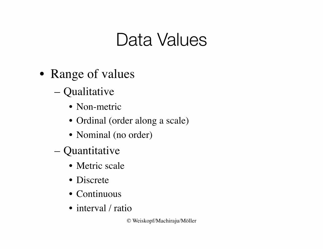
• Range of values – Qualitative
• Non-metric• Ordinal (order along a scale)• Nominal (no order)
– Quantitative• Metric scale• Discrete• Continuous• interval / ratio
© Weiskopf/Machiraju/Möller
Data Types
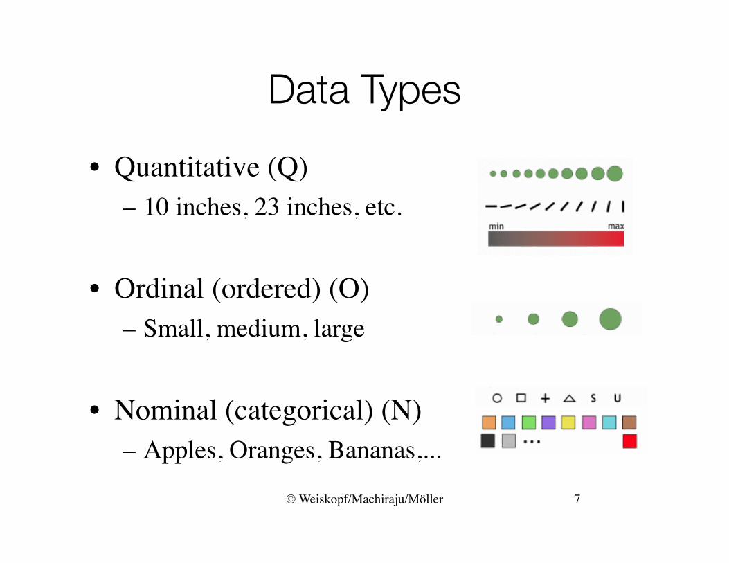
• Quantitative (Q)– 10 inches, 23 inches, etc.
• Ordinal (ordered) (O)– Small, medium, large
• Nominal (categorical) (N)– Apples, Oranges, Bananas,...
7
© Weiskopf/Machiraju/Möller
Quantitative
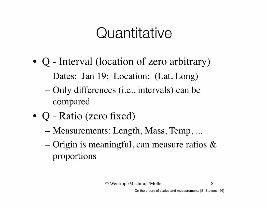
• Q - Interval (location of zero arbitrary)– Dates: Jan 19; Location: (Lat, Long)– Only differences (i.e., intervals) can be
compared• Q - Ratio (zero fixed)
– Measurements: Length, Mass, Temp, ...– Origin is meaningful, can measure ratios &
proportions
8On the theory of scales and measurements [S. Stevens, 46]
© Weiskopf/Machiraju/Möller
Quantitative
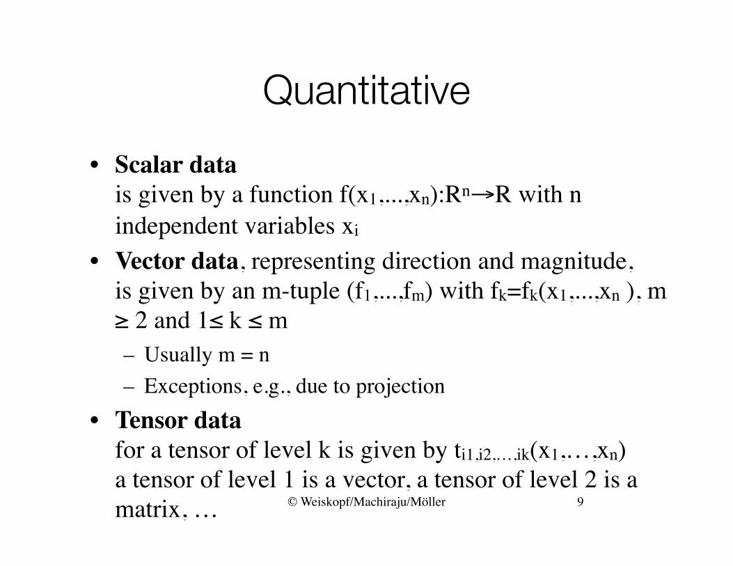
• Scalar datais given by a function f(x1,...,xn):Rn→R with n independent variables xi
• Vector data, representing direction and magnitude, is given by an m-tuple (f1,...,fm) with fk=fk(x1,...,xn ), m ≥ 2 and 1≤ k ≤ m– Usually m = n– Exceptions, e.g., due to projection
• Tensor datafor a tensor of level k is given by ti1,i2,…,ik(x1,…,xn)a tensor of level 1 is a vector, a tensor of level 2 is a matrix, … 9
© Weiskopf/Machiraju/Möller
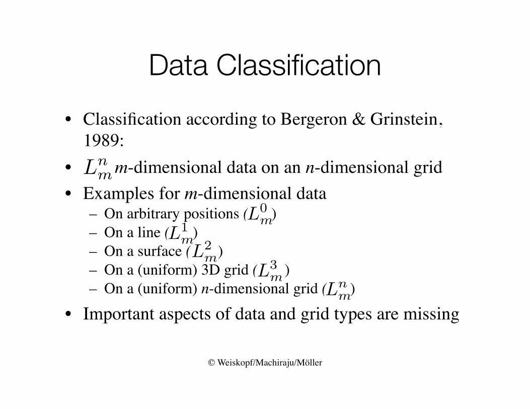
Data Classification
• Classification according to Bergeron & Grinstein,1989:
• m-dimensional data on an n-dimensional grid• Examples for m-dimensional data
– On arbitrary positions ( )– On a line ( )– On a surface ( )– On a (uniform) 3D grid ( )– On a (uniform) n-dimensional grid ( )
• Important aspects of data and grid types are missing
Lnm
L0m
L1mL2
mL3
mLn
m
© Weiskopf/Machiraju/Möller
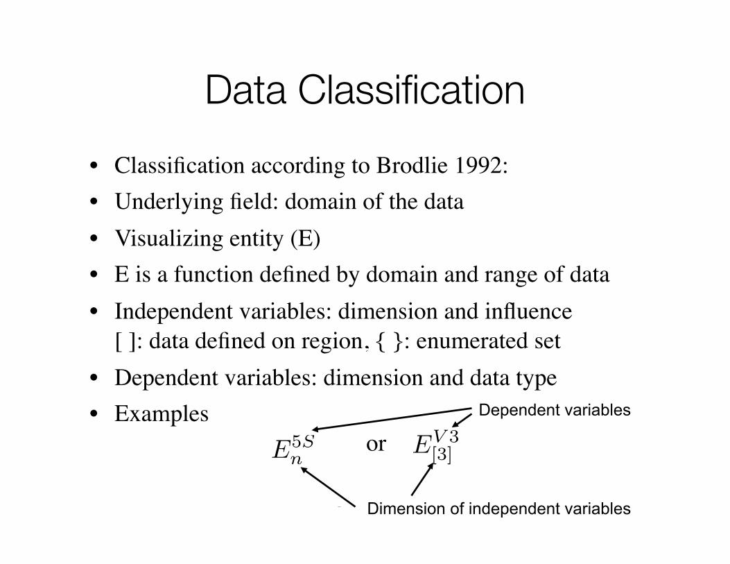
Data Classification
• Classification according to Brodlie 1992:• Underlying field: domain of the data• Visualizing entity (E)• E is a function defined by domain and range of data• Independent variables: dimension and influence
[ ]: data defined on region, { }: enumerated set• Dependent variables: dimension and data type• Examples
or
Dimension of independent variables
Dependent variables
E5Sn
EV 3[3]
© Weiskopf/Machiraju/Möller
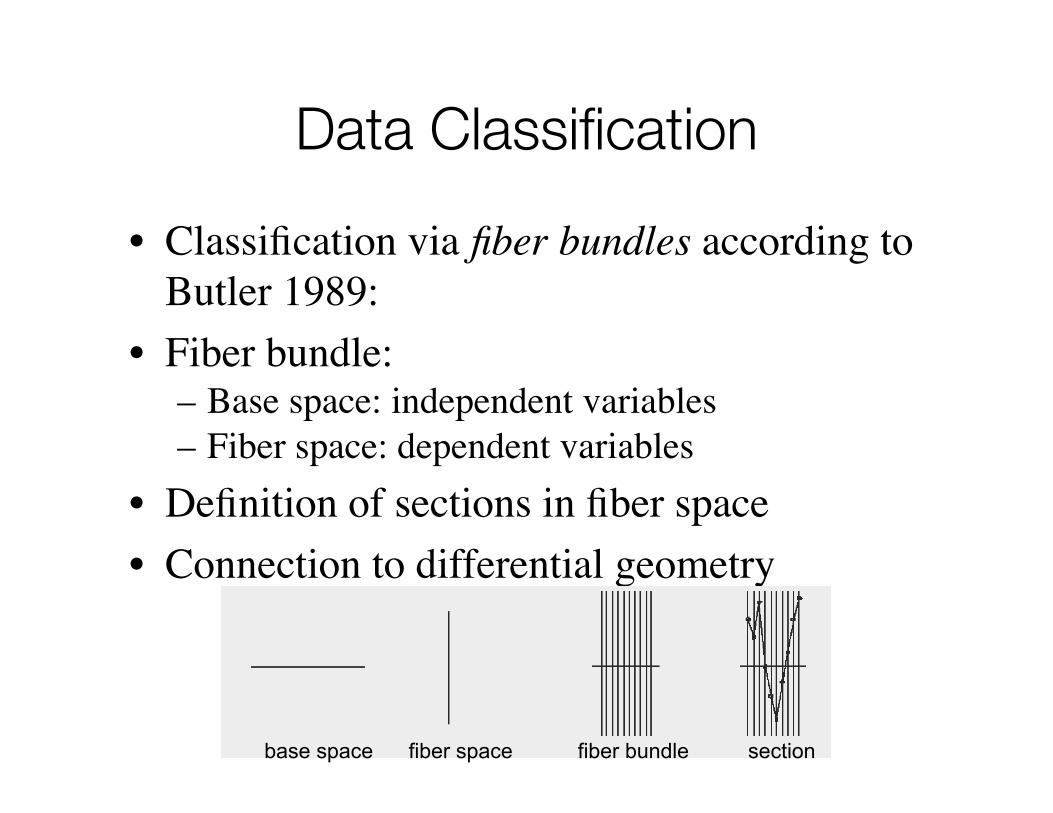
Data Classification
• Classification via fiber bundles according to Butler 1989:
• Fiber bundle:– Base space: independent variables– Fiber space: dependent variables
• Definition of sections in fiber space• Connection to differential geometry
base space fiber space fiber bundle section
© Weiskopf/Machiraju/Möller
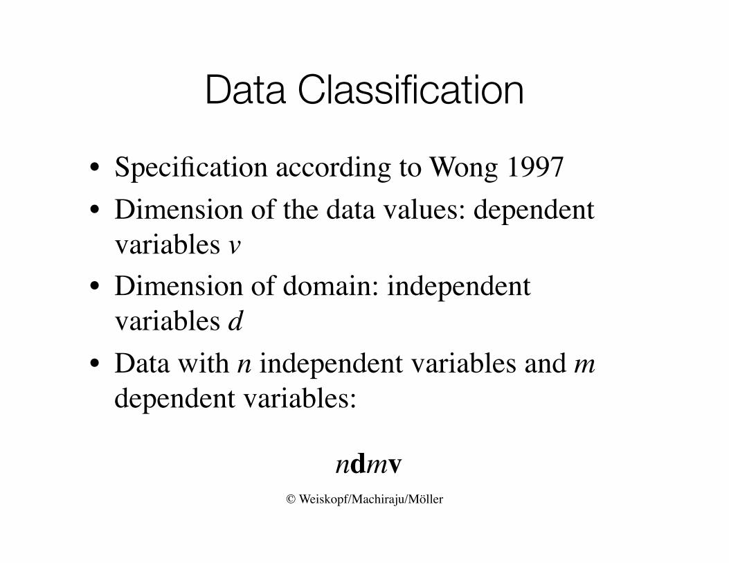
Data Classification
• Specification according to Wong 1997• Dimension of the data values: dependent
variables v• Dimension of domain: independent
variables d• Data with n independent variables and m
dependent variables:
ndmv
© Weiskopf/Machiraju/Möller
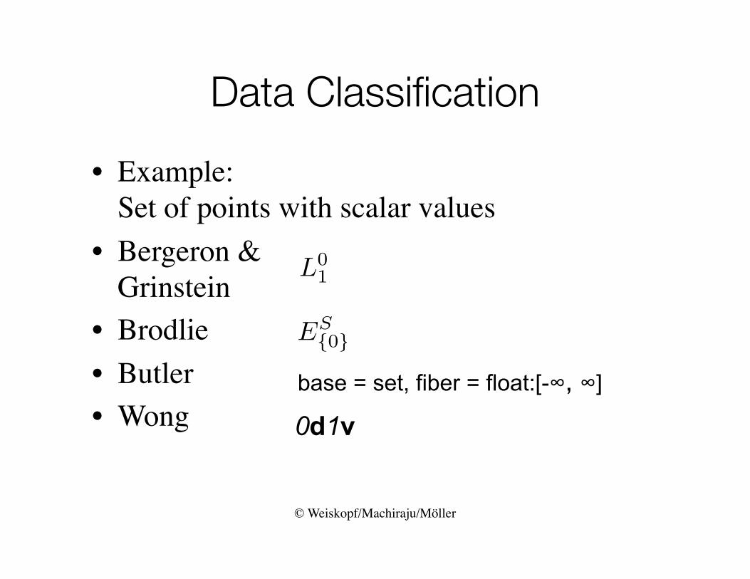
Data Classification
• Example:Set of points with scalar values
• Bergeron & Grinstein
• Brodlie• Butler• Wong
base = set, fiber = float:[-∞, ∞]
0d1v
ES{0}
L01
© Weiskopf/Machiraju/Möller
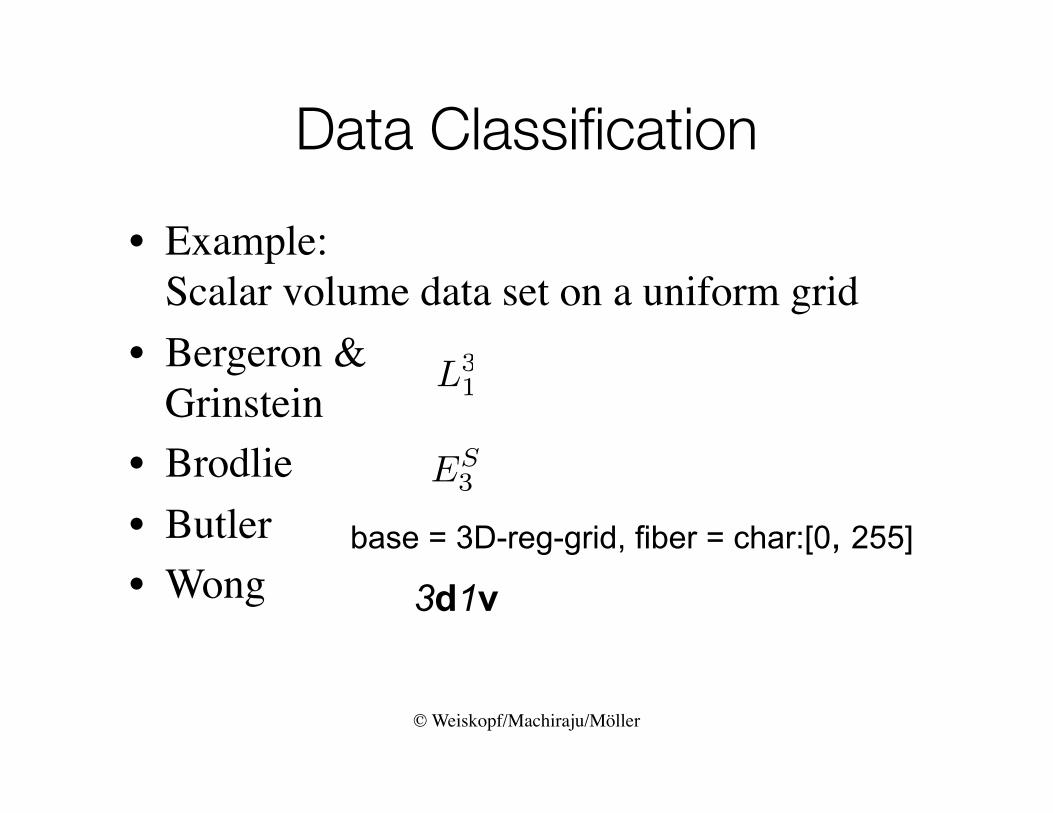
Data Classification
• Example:Scalar volume data set on a uniform grid
• Bergeron & Grinstein
• Brodlie• Butler• Wong
base = 3D-reg-grid, fiber = char:[0, 255]
3d1v
L31
ES3
© Weiskopf/Machiraju/Möller
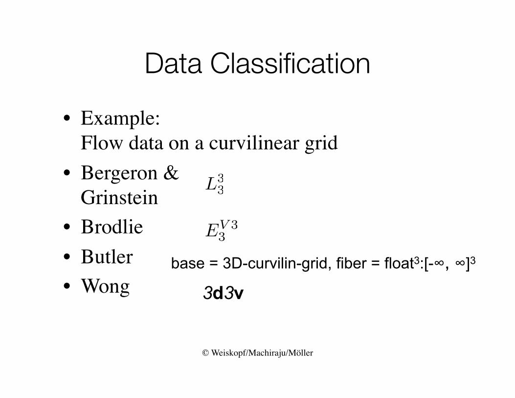
Data Classification
• Example:Flow data on a curvilinear grid
• Bergeron & Grinstein
• Brodlie• Butler• Wong
base = 3D-curvilin-grid, fiber = float3:[-∞, ∞]3
3d3v
EV 33
L33
© Weiskopf/Machiraju/Möller
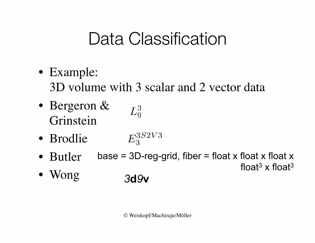
Data Classification
• Example:3D volume with 3 scalar and 2 vector data
• Bergeron & Grinstein
• Brodlie• Butler• Wong
base = 3D-reg-grid, fiber = float x float x float x float3 x float3
3d9v
L39
E3S2V 33
© Weiskopf/Machiraju/Möller
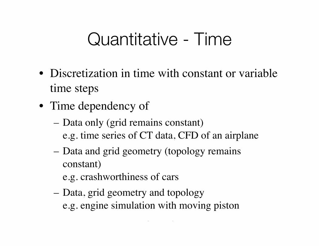
Quantitative - Time
• Discretization in time with constant or variable time steps
• Time dependency of– Data only (grid remains constant)
e.g. time series of CT data, CFD of an airplane– Data and grid geometry (topology remains
constant)e.g. crashworthiness of cars
– Data, grid geometry and topologye.g. engine simulation with moving piston
Data Structure
© Weiskopf/Machiraju/Möller
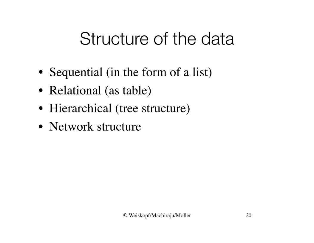
Structure of the data
• Sequential (in the form of a list)• Relational (as table)• Hierarchical (tree structure)• Network structure
20
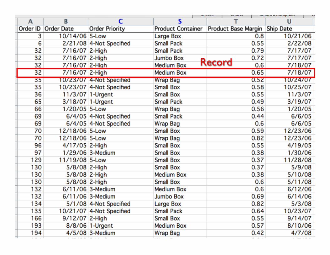
Record
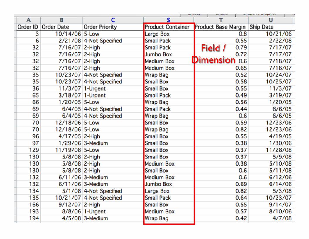
Field / Dimension
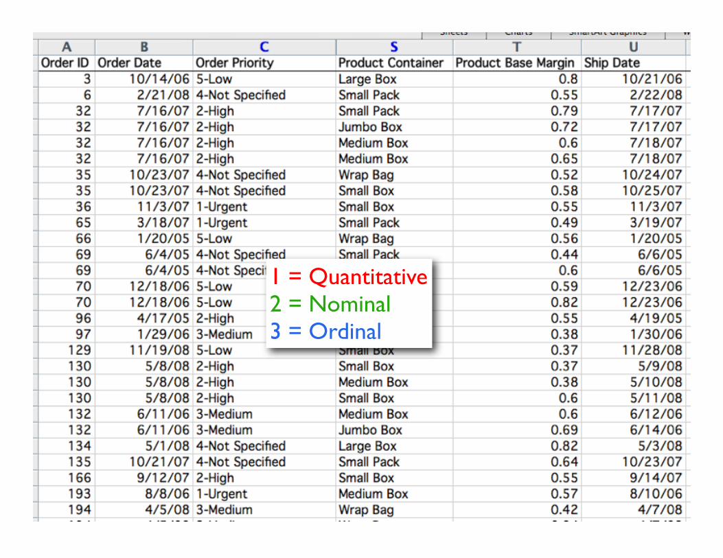
1 = Quantitative2 = Nominal3 = Ordinal
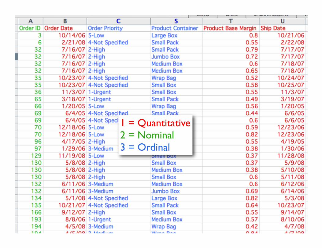
1 = Quantitative2 = Nominal3 = Ordinal
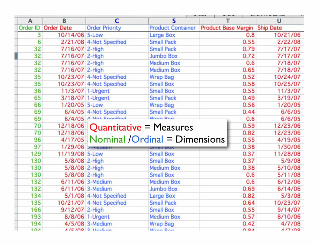
Quantitative = MeasuresNominal /Ordinal = Dimensions
© Weiskopf/Machiraju/Möller
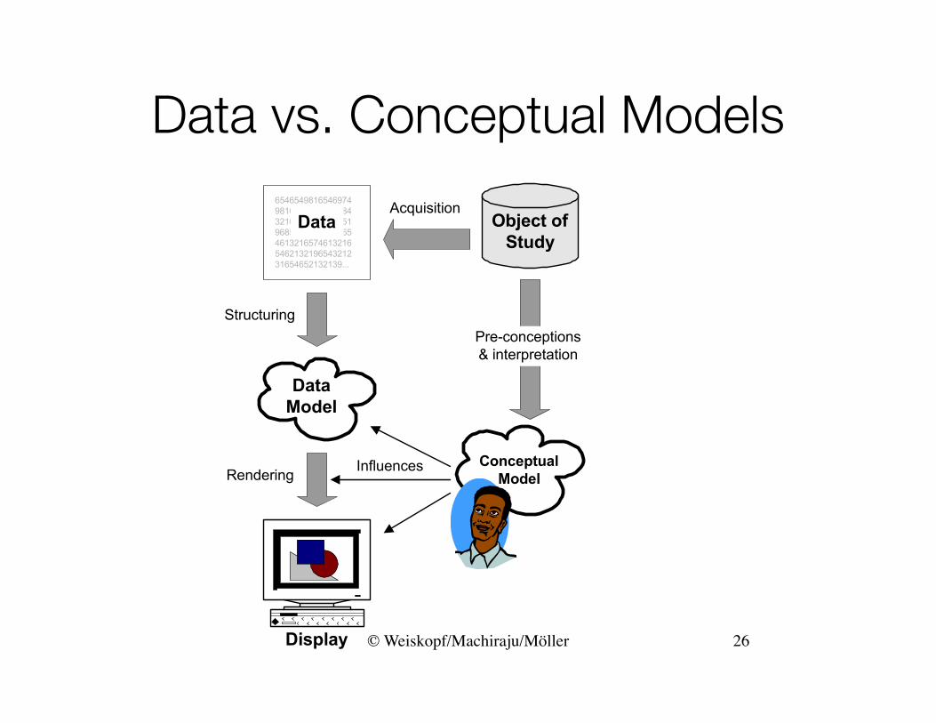
Data vs. Conceptual Models
26
© Weiskopf/Machiraju/Möller
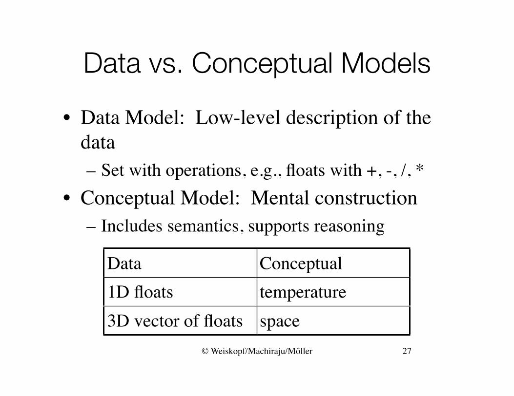
Data vs. Conceptual Models
• Data Model: Low-level description of the data – Set with operations, e.g., floats with +, -, /, *
• Conceptual Model: Mental construction– Includes semantics, supports reasoning
Data Conceptual1D floats temperature3D vector of floats space
27
© Weiskopf/Machiraju/Möller
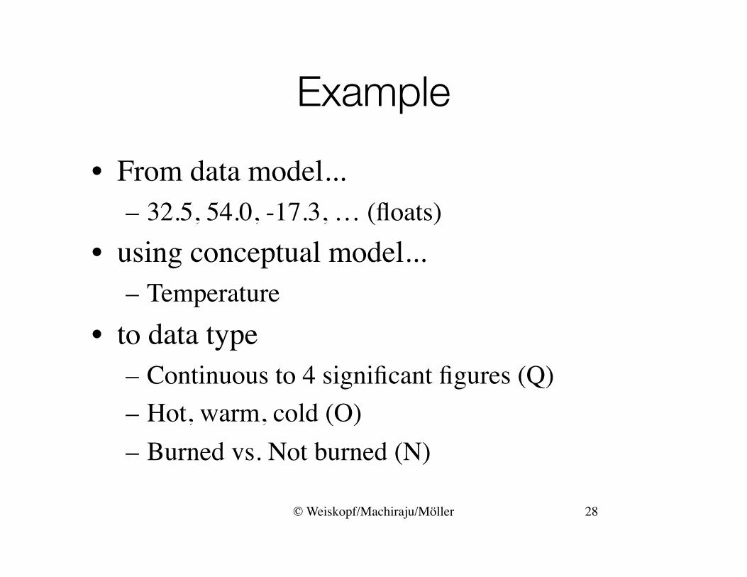
Example
• From data model...– 32.5, 54.0, -17.3, … (floats)
• using conceptual model...– Temperature
• to data type– Continuous to 4 significant figures (Q) – Hot, warm, cold (O) – Burned vs. Not burned (N)
28
© Weiskopf/Machiraju/Möller
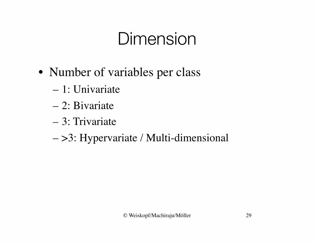
Dimension
• Number of variables per class– 1: Univariate– 2: Bivariate– 3: Trivariate– >3: Hypervariate / Multi-dimensional
29

Visualization Flavours
© Weiskopf/Machiraju/Möller
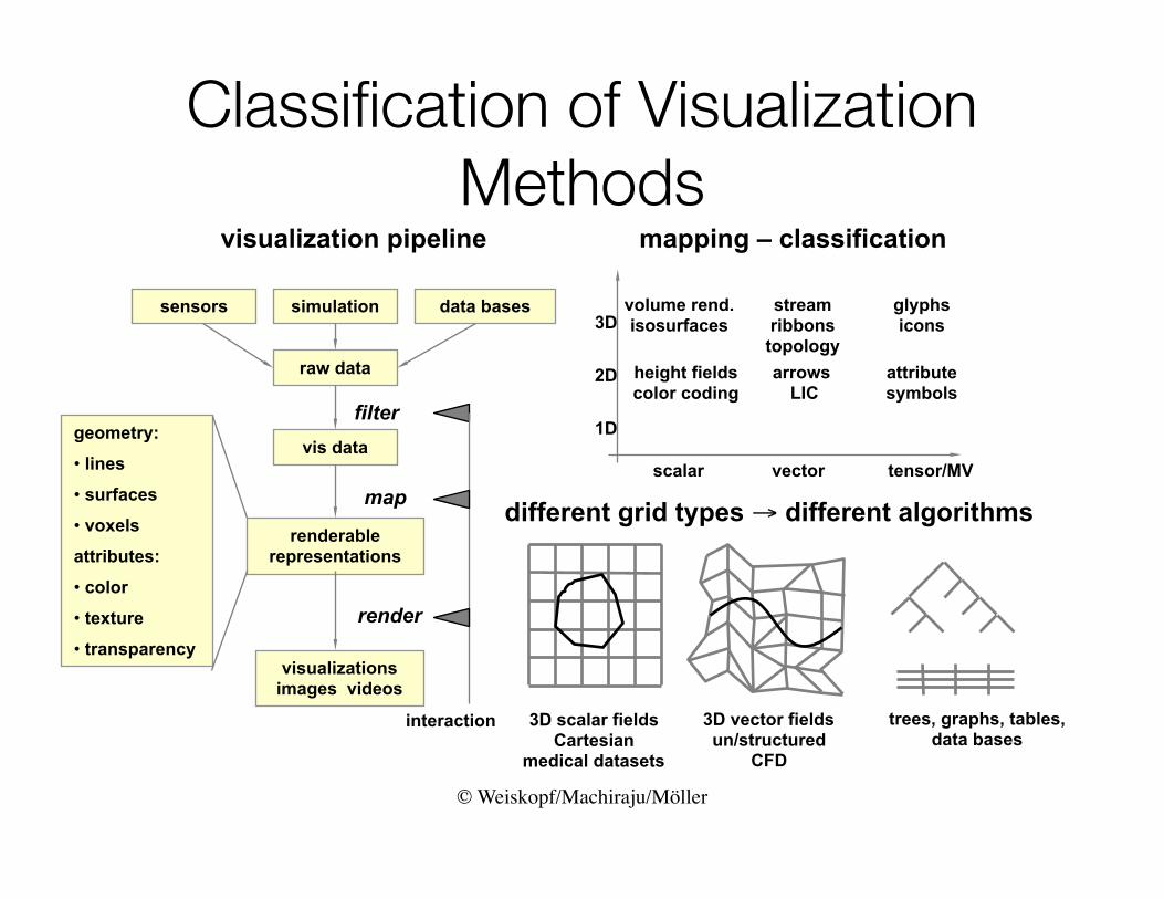
Classification of Visualization Methods
sensors data basessimulation
raw data
vis data
renderable representations
visualizations images videos
geometry:
• lines
• surfaces
• voxels
attributes:
• color
• texture
• transparency
filter
render
map
interaction
visualization pipeline mapping – classification
1D
3D
2D
scalar vector tensor/MV
volume rend. isosurfaces
height fields color coding
stream ribbonstopologyarrows
LICattribute symbols
glyphs icons
different grid types → different algorithms
3D scalar fields Cartesian
medical datasets
3D vector fields un/structured
CFD
trees, graphs, tables, data bases
© Weiskopf/Machiraju/Möller
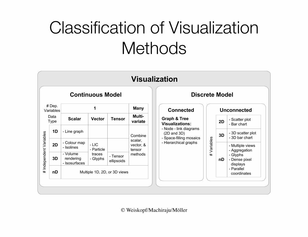
Classification of Visualization Methods
© Weiskopf/Machiraju/Möller
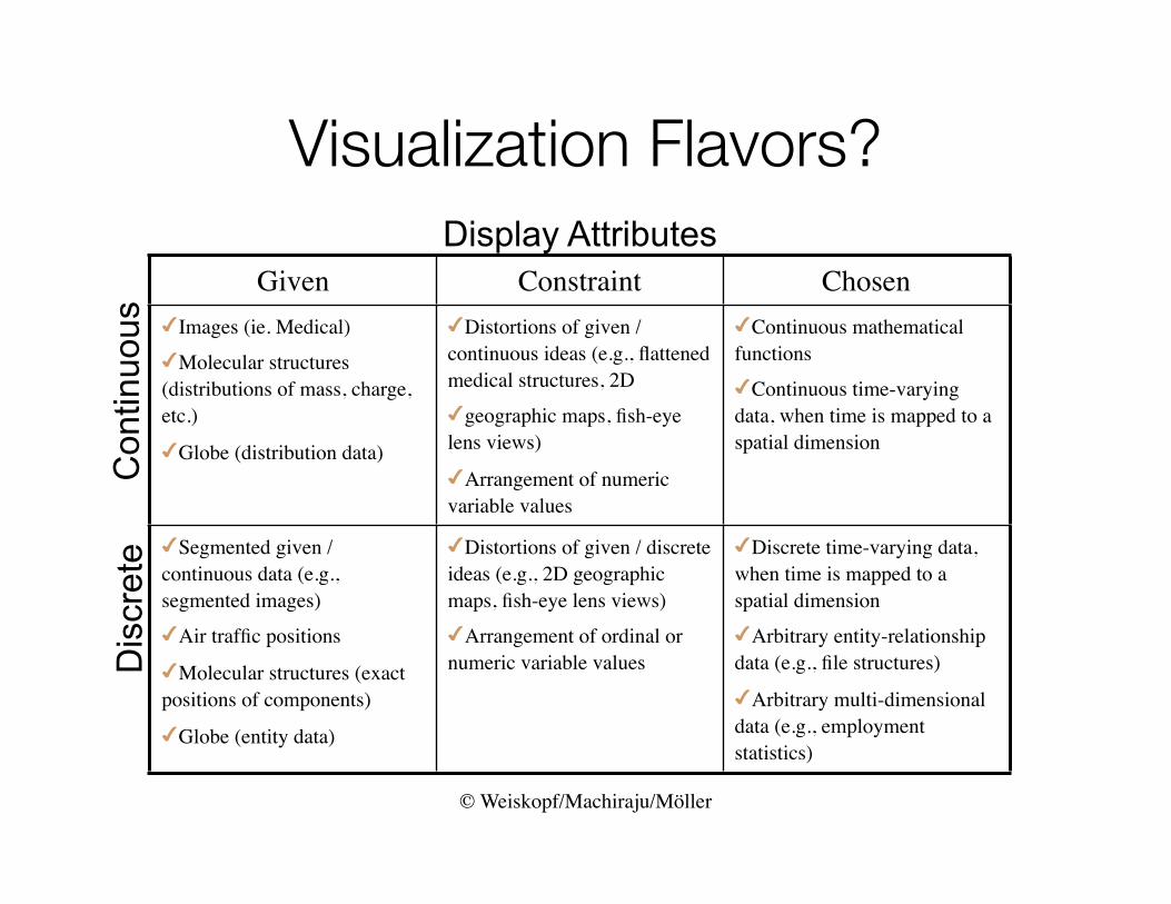
Visualization Flavors?
Given Constraint ChosenImages (ie. Medical)Molecular structures (distributions of mass, charge, etc.)Globe (distribution data)
Distortions of given / continuous ideas (e.g., flattened medical structures, 2Dgeographic maps, fish-eye lens views)Arrangement of numeric variable values
Continuous mathematical functionsContinuous time-varying data, when time is mapped to a spatial dimension
Segmented given / continuous data (e.g., segmented images)Air traffic positionsMolecular structures (exact positions of components)Globe (entity data)
Distortions of given / discrete ideas (e.g., 2D geographic maps, fish-eye lens views)Arrangement of ordinal or numeric variable values
Discrete time-varying data, when time is mapped to a spatial dimensionArbitrary entity-relationship data (e.g., file structures)Arbitrary multi-dimensional data (e.g., employment statistics)
Display Attributes
Con
tinuo
usD
iscr
ete
© Weiskopf/Machiraju/Möller
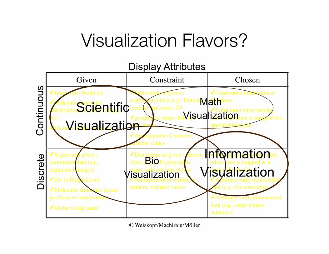
Visualization Flavors?
Given Constraint ChosenImages (ie. Medical)Molecular structures (distributions of mass, charge, etc.)Globe (distribution data)
Distortions of given / continuous ideas (e.g., flattened medical structures, 2Dgeographic maps, fish-eye lens views)Arrangement of numeric variable values
Continuous mathematical functionsContinuous time-varying data, when time is mapped to a spatial dimension
Segmented given / continuous data (e.g., segmented images)Air traffic positionsMolecular structures (exact positions of components)Globe (entity data)
Distortions of given / discrete ideas (e.g., 2D geographic maps, fish-eye lens views)Arrangement of ordinal or numeric variable values
Discrete time-varying data, when time is mapped to a spatial dimensionArbitrary entity-relationship data (e.g., file structures)Arbitrary multi-dimensional data (e.g., employment statistics)
Display Attributes
Con
tinuo
usD
iscr
ete Information
Visualization
MathVisualization
ScientificVisualization
BioVisualization

Task Abstraction

Task Abstraction
[Meyer et al., MizBee: A Multiscale Synteny Browser, 2009]
© Weiskopf/Machiraju/Möller
Task Abstraction
37
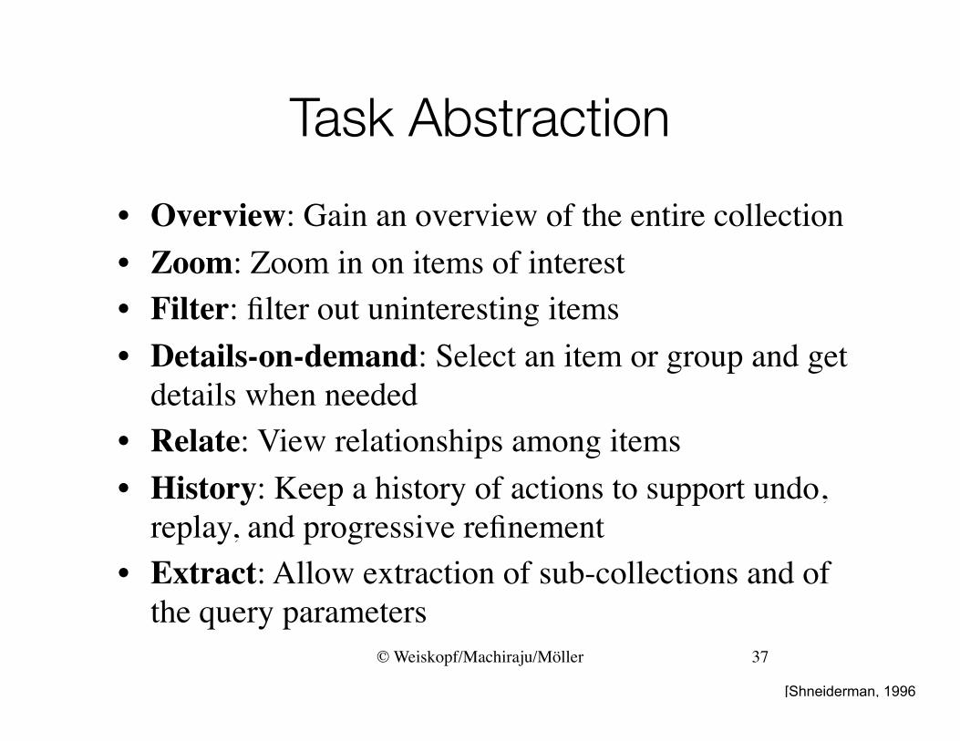
• Overview: Gain an overview of the entire collection• Zoom: Zoom in on items of interest• Filter: filter out uninteresting items• Details-on-demand: Select an item or group and get
details when needed• Relate: View relationships among items• History: Keep a history of actions to support undo,
replay, and progressive refinement• Extract: Allow extraction of sub-collections and of
the query parameters
[Shneiderman, 1996]
© Weiskopf/Machiraju/Möller
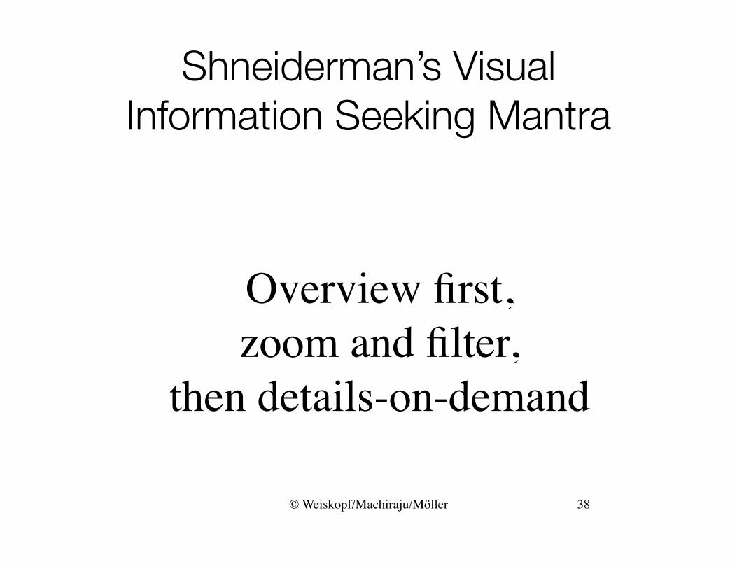
Shneiderman’s Visual Information Seeking Mantra
Overview first,zoom and filter,
then details-on-demand
38
© Weiskopf/Machiraju/Möller
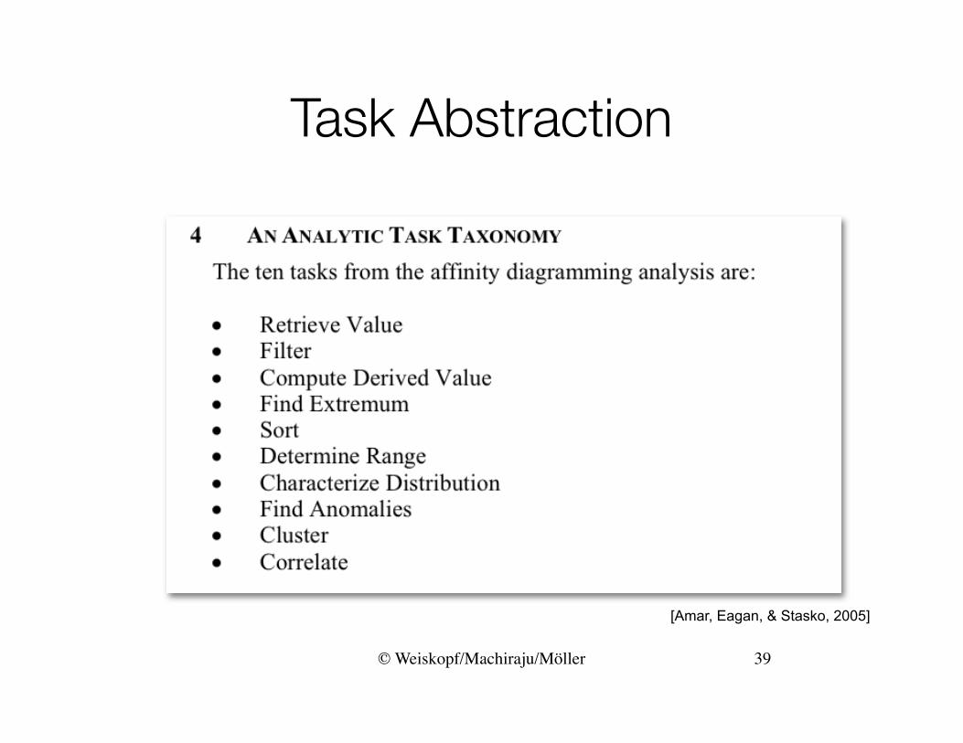
Task Abstraction
[Amar, Eagan, & Stasko, 2005]
39
© Weiskopf/Machiraju/Möller
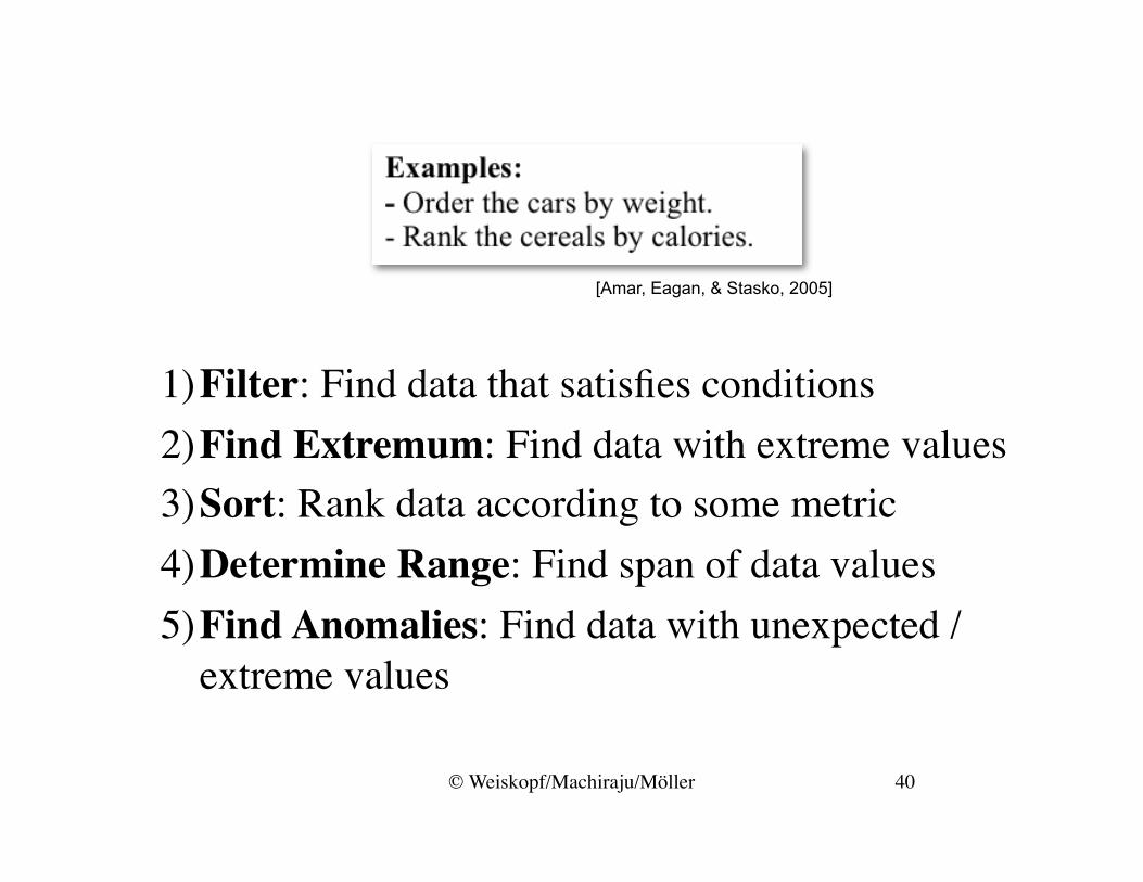
1)Filter: Find data that satisfies conditions2)Find Extremum: Find data with extreme values3)Sort: Rank data according to some metric4)Determine Range: Find span of data values5)Find Anomalies: Find data with unexpected /
extreme values
[Amar, Eagan, & Stasko, 2005]
40
© Weiskopf/Machiraju/Möller
Data Types, Sources, and Tasks
• Data Types• Data Structures• Data vs. Conceptual Model• Data classification• Classification of visualization methods• Tasks• Continuous Data
– Data sources– Data acquisition with scanners– Sources of Error– Data representation– Domain– Data structures
© Weiskopf/Machiraju/Möller
Data Sources
• The capability of traditional presentation techniques is not sufficient for the increasing amount of data to be interpreted– Data might come from any source with almost arbitrary size– Techniques to efficiently visualize large-scale data sets and new
data types need to be developed
• Real world– Measurements and observation
• Theoretical world– Mathematical and technical models
• Artificial world– Data that is designed
© Weiskopf/Machiraju/Möller
TB
GB
MB
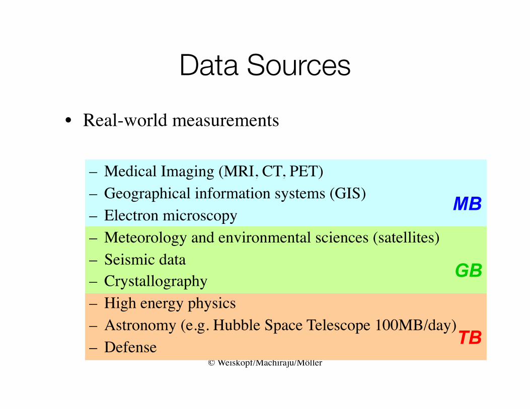
Data Sources
• Real-world measurements
– Medical Imaging (MRI, CT, PET)– Geographical information systems (GIS)– Electron microscopy– Meteorology and environmental sciences (satellites)– Seismic data– Crystallography– High energy physics– Astronomy (e.g. Hubble Space Telescope 100MB/day)– Defense
© Weiskopf/Machiraju/MöllerMBGB
GB
MB
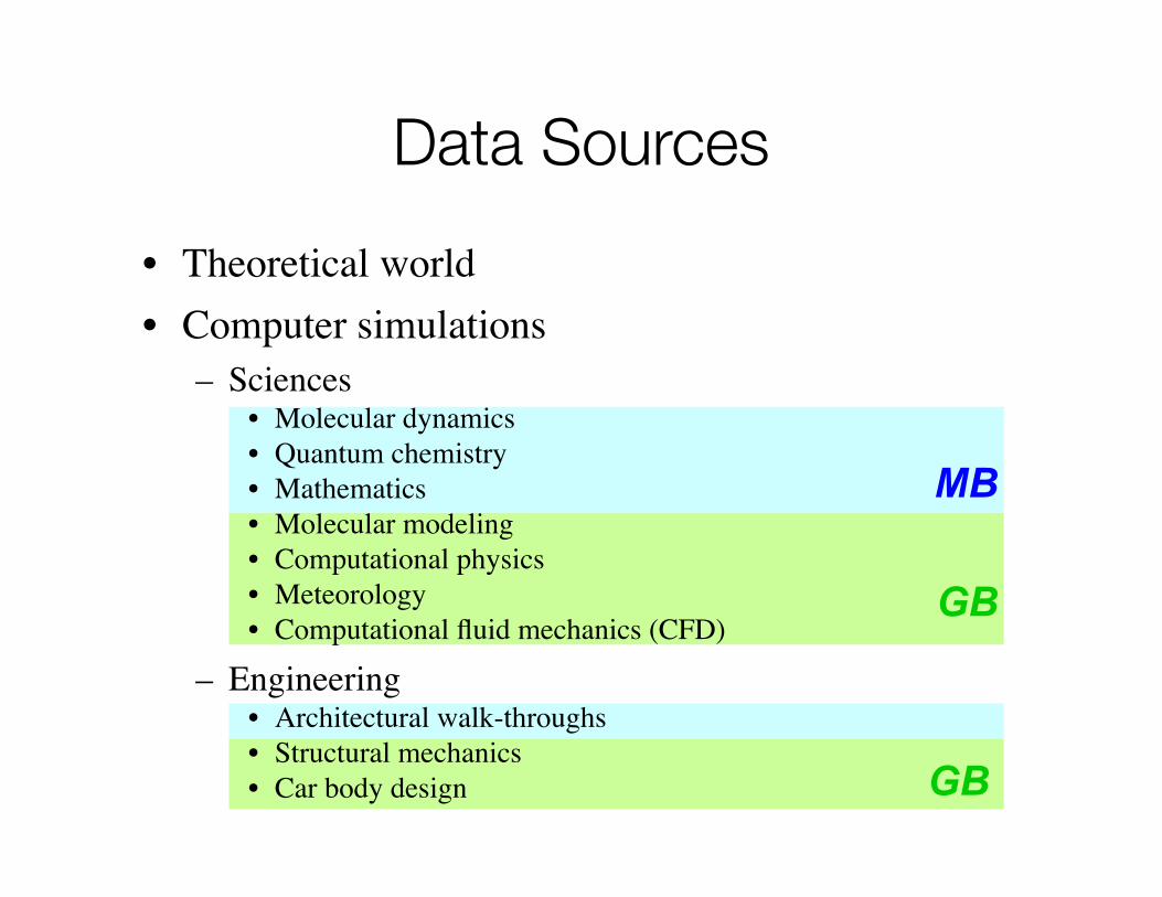
Data Sources
• Theoretical world• Computer simulations
– Sciences• Molecular dynamics• Quantum chemistry• Mathematics• Molecular modeling• Computational physics• Meteorology• Computational fluid mechanics (CFD)
– Engineering• Architectural walk-throughs• Structural mechanics• Car body design
© Weiskopf/Machiraju/Möller
TB
Data Sources
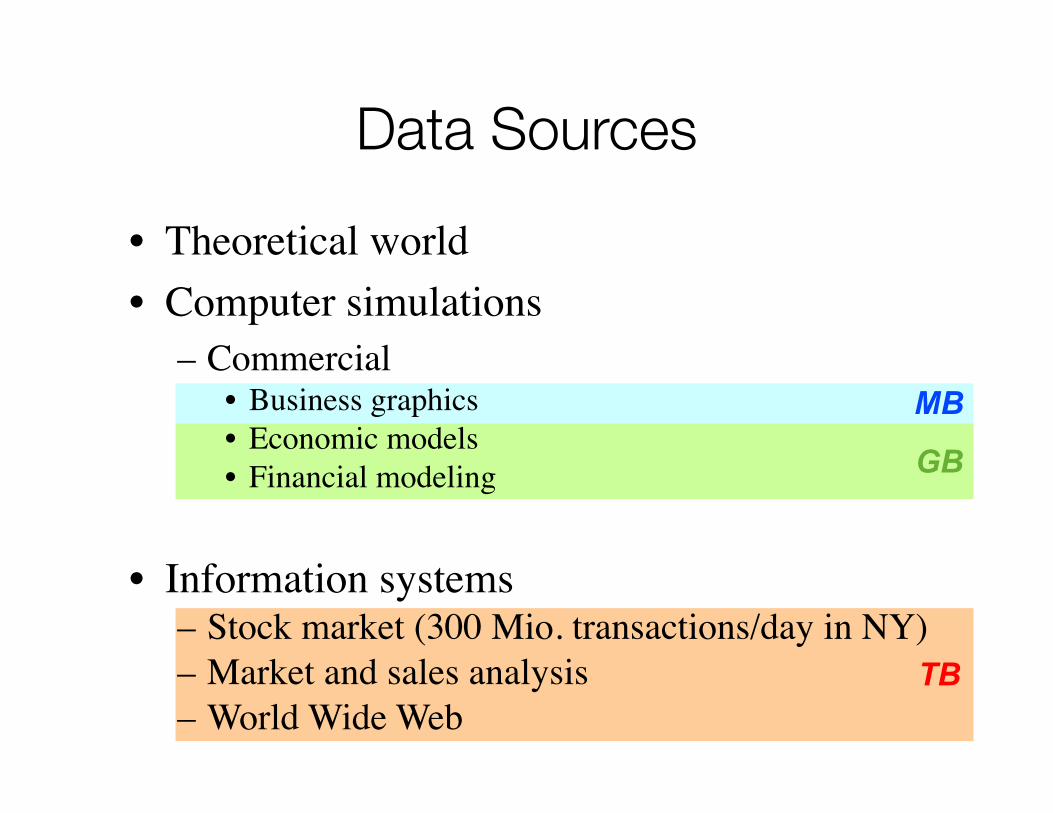
• Theoretical world• Computer simulations
– Commercial • Business graphics• Economic models• Financial modeling
• Information systems– Stock market (300 Mio. transactions/day in NY)– Market and sales analysis– World Wide Web
MB
GB
© Weiskopf/Machiraju/Möller
Data Sources
TB
MB
GB
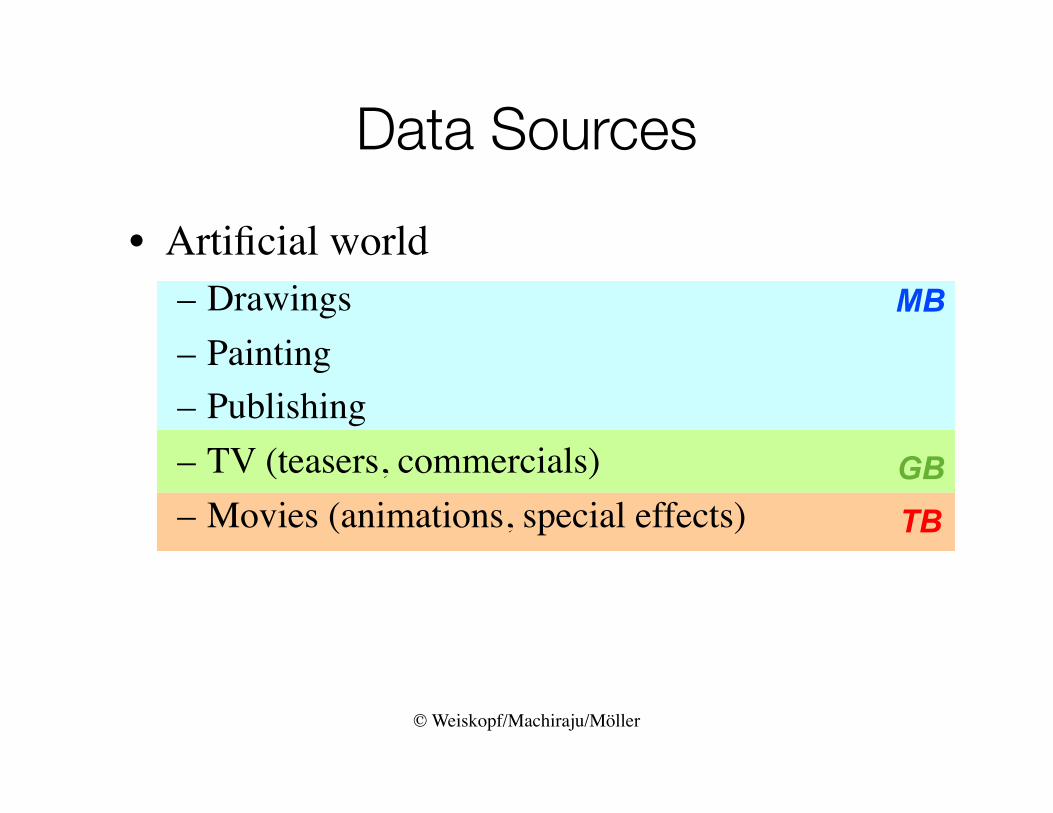
• Artificial world– Drawings– Painting– Publishing– TV (teasers, commercials)– Movies (animations, special effects)
© Weiskopf/Machiraju/Möller
Data Acquisition with Scanners
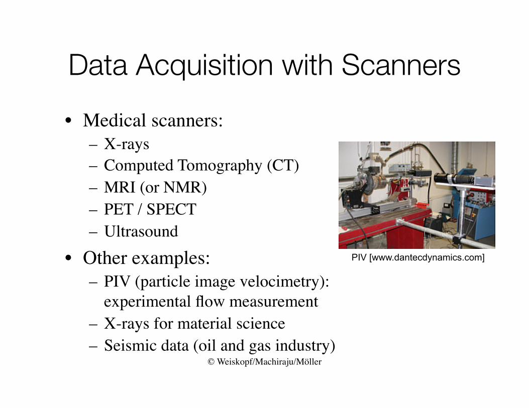
• Medical scanners:– X-rays– Computed Tomography (CT)– MRI (or NMR)– PET / SPECT– Ultrasound
• Other examples:– PIV (particle image velocimetry):
experimental flow measurement– X-rays for material science– Seismic data (oil and gas industry)
PIV [www.dantecdynamics.com]
© Weiskopf/Machiraju/Möller
Data Acquisition with Scanners
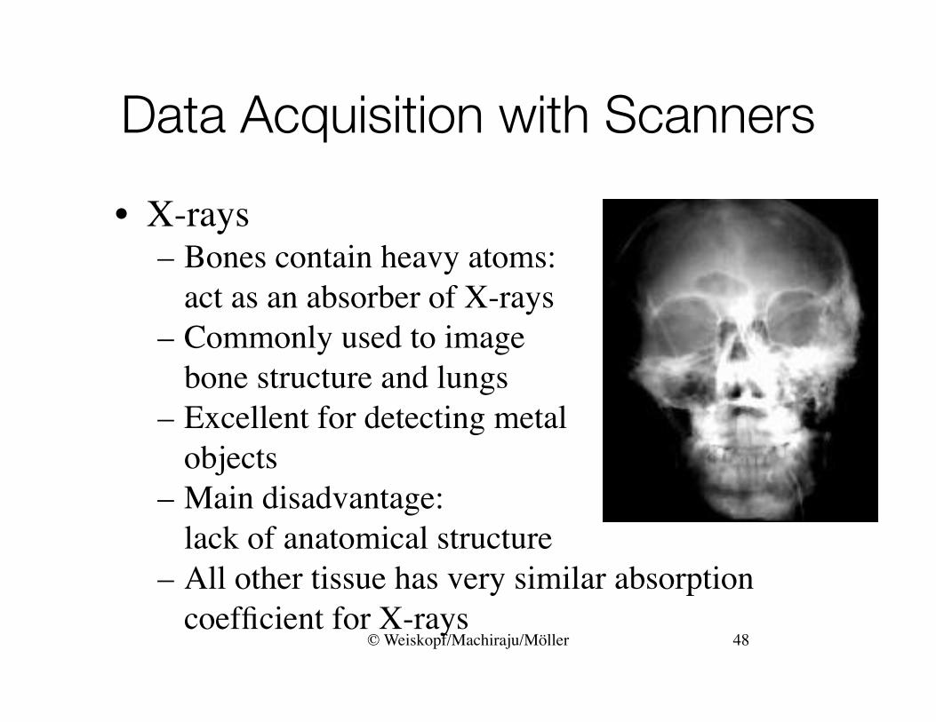
• X-rays– Bones contain heavy atoms:
act as an absorber of X-rays– Commonly used to image
bone structure and lungs– Excellent for detecting metal
objects– Main disadvantage:
lack of anatomical structure – All other tissue has very similar absorption
coefficient for X-rays48
© Weiskopf/Machiraju/Möller
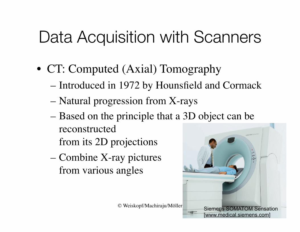
Data Acquisition with Scanners
• CT: Computed (Axial) Tomography– Introduced in 1972 by Hounsfield and Cormack– Natural progression from X-rays– Based on the principle that a 3D object can be
reconstructed from its 2D projections
– Combine X-ray pictures from various angles
Siemens SOMATOM Sensation[www.medical.siemens.com]
© Weiskopf/Machiraju/Möller
Data Acquisition with Scanners
• CT: Computed (Axial) Tomography• Advantages
– Superior to single X-ray scans – Easier to separate soft tissues (materials other
than bone) from one another (e.g. liver, kidney)– Data exist in digital form: can be analyzed
quantitatively• Disadvantages
– Significantly more data collected– Soft tissue X-ray absorption still relatively similar– A health risk
© Weiskopf/Machiraju/Möller
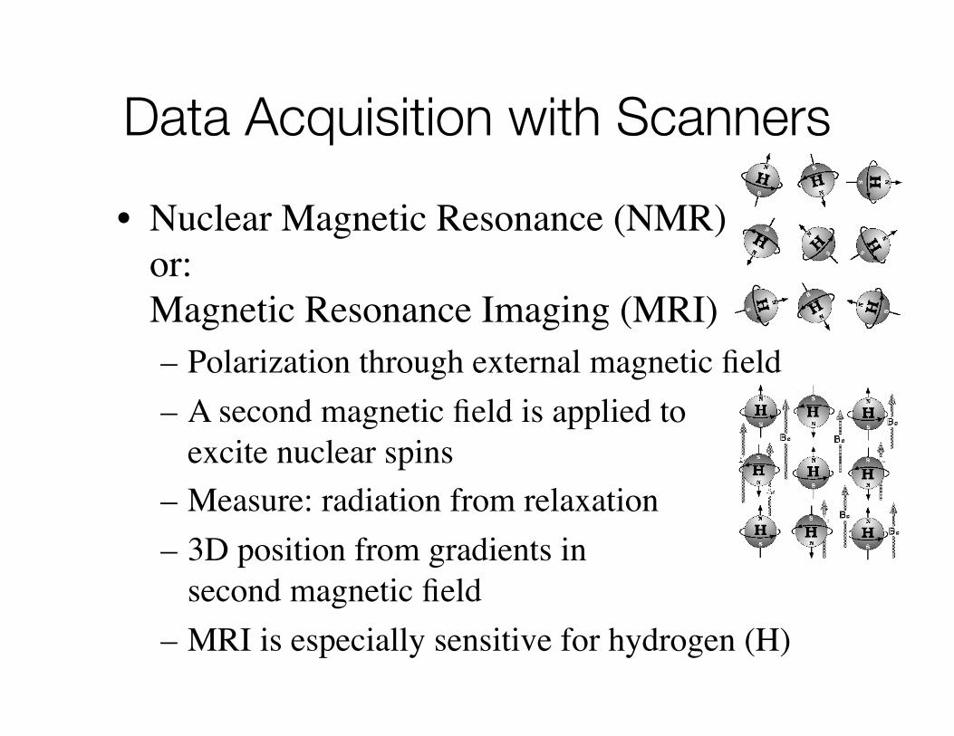
Data Acquisition with Scanners
• Nuclear Magnetic Resonance (NMR) - or:Magnetic Resonance Imaging (MRI)– Polarization through external magnetic field– A second magnetic field is applied to
excite nuclear spins– Measure: radiation from relaxation– 3D position from gradients in
second magnetic field – MRI is especially sensitive for hydrogen (H)

© Weiskopf/Machiraju/Möller
Data Acquisition with Scanners
• MRI / NRM advantages:– Detailed anatomical information– High-energy radiation is
not used, i.e. “safe” scanning method
– (Medicine) uses resonance properties of protons
Siemens MAGNETOM Allegra 3T Brainscanner[www.medical.siemens.com]
© Weiskopf/Machiraju/Möller
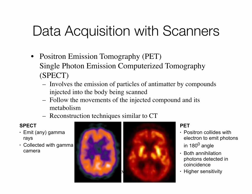
Data Acquisition with Scanners
• Positron Emission Tomography (PET)Single Photon Emission Computerized Tomography (SPECT)– Involves the emission of particles of antimatter by compounds
injected into the body being scanned– Follow the movements of the injected compound and its
metabolism– Reconstruction techniques similar to CT
SPECT• Emit (any) gamma
rays• Collected with gamma
camera
PET• Positron collides with
electron to emit photons in 1800 angle
• Both annihilation photons detected in coincidence
• Higher sensitivity
© Weiskopf/Machiraju/Möller
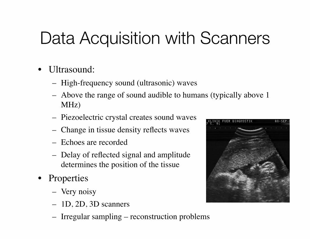
Data Acquisition with Scanners
• Ultrasound:– High-frequency sound (ultrasonic) waves– Above the range of sound audible to humans (typically above 1
MHz)– Piezoelectric crystal creates sound waves– Change in tissue density reflects waves– Echoes are recorded– Delay of reflected signal and amplitude
determines the position of the tissue
• Properties– Very noisy– 1D, 2D, 3D scanners– Irregular sampling – reconstruction problems
© Weiskopf/Machiraju/Möller
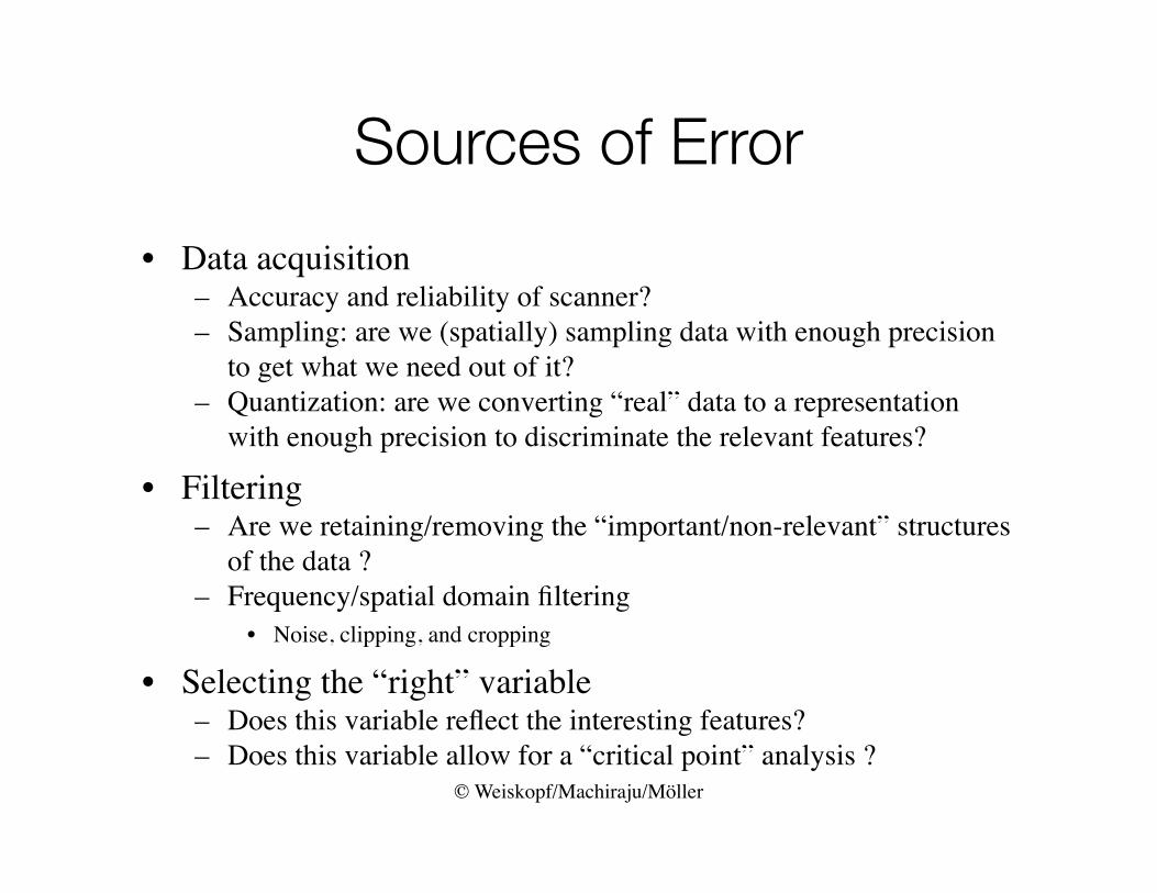
Sources of Error
• Data acquisition– Accuracy and reliability of scanner?– Sampling: are we (spatially) sampling data with enough precision
to get what we need out of it?– Quantization: are we converting “real” data to a representation
with enough precision to discriminate the relevant features?
• Filtering– Are we retaining/removing the “important/non-relevant” structures
of the data ?– Frequency/spatial domain filtering
• Noise, clipping, and cropping
• Selecting the “right” variable – Does this variable reflect the interesting features?– Does this variable allow for a “critical point” analysis ?
© Weiskopf/Machiraju/Möller
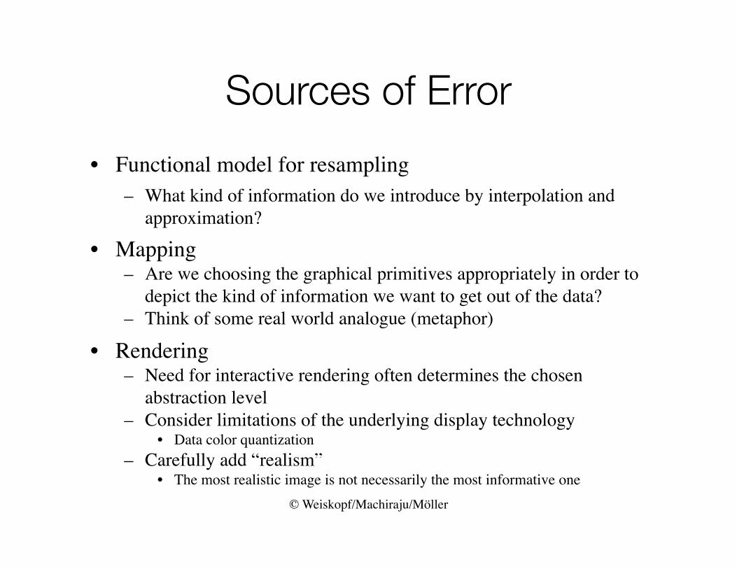
Sources of Error
• Functional model for resampling– What kind of information do we introduce by interpolation and
approximation?
• Mapping– Are we choosing the graphical primitives appropriately in order to
depict the kind of information we want to get out of the data?– Think of some real world analogue (metaphor)
• Rendering– Need for interactive rendering often determines the chosen
abstraction level– Consider limitations of the underlying display technology
• Data color quantization– Carefully add “realism”
• The most realistic image is not necessarily the most informative one
© Weiskopf/Machiraju/Möller
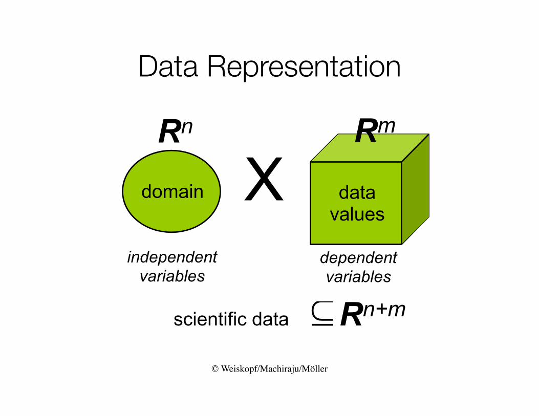
Data Representation
domain
independentvariables
Rn
data values
Xdependentvariables
Rm
scientific data Rn+m
© Weiskopf/Machiraju/Möller
Data Representation
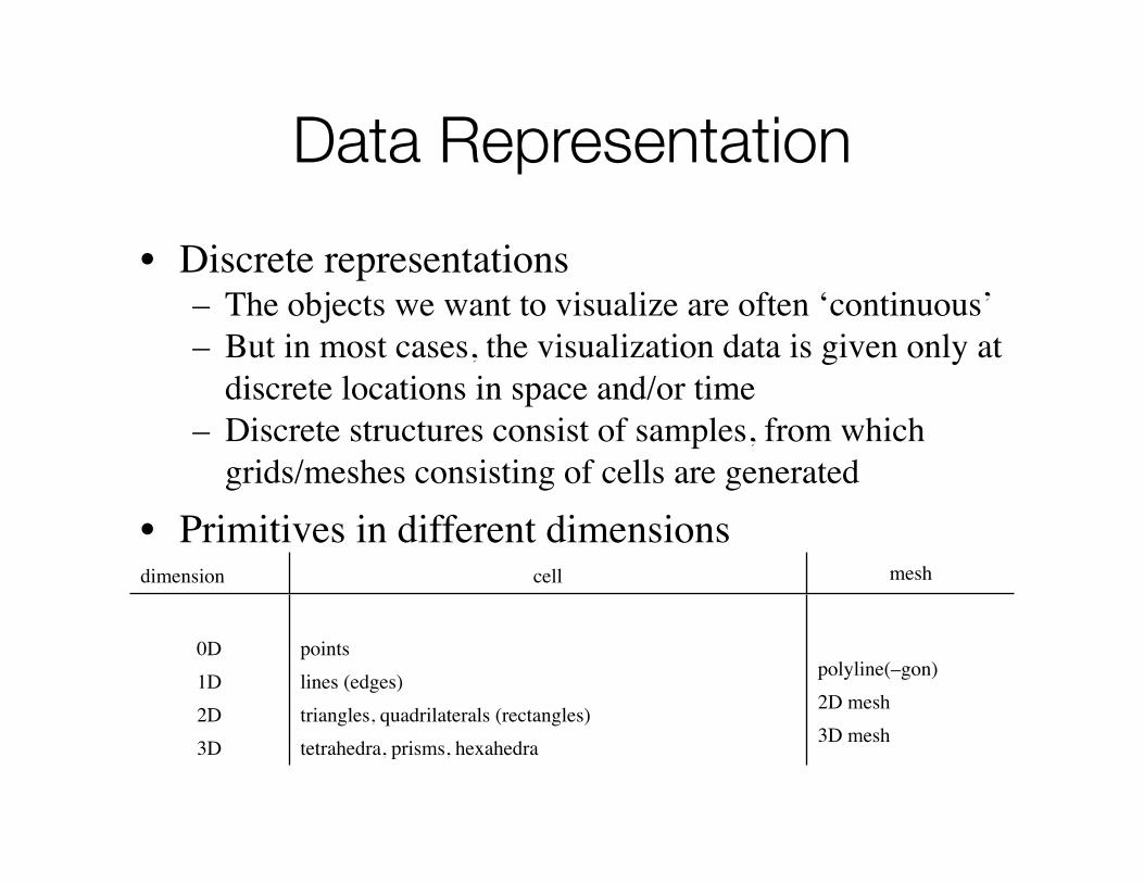
• Discrete representations– The objects we want to visualize are often ‘continuous’– But in most cases, the visualization data is given only at
discrete locations in space and/or time– Discrete structures consist of samples, from which
grids/meshes consisting of cells are generated
• Primitives in different dimensionsdimension cell mesh
0D1D2D3D
pointslines (edges)triangles, quadrilaterals (rectangles)tetrahedra, prisms, hexahedra
polyline(–gon)2D mesh3D mesh
© Weiskopf/Machiraju/Möller
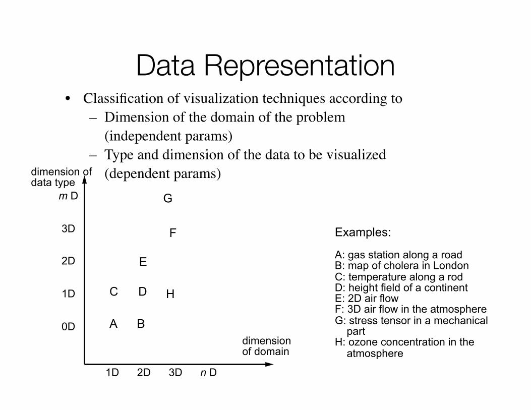
Data Representation• Classification of visualization techniques according to
– Dimension of the domain of the problem (independent params)
– Type and dimension of the data to be visualized (dependent params)
m D
3D
2D
1D
0D
1D 2D 3D n D
dimension of domain
G
C D
A B
F
E
H
Examples:
A: gas station along a roadB: map of cholera in LondonC: temperature along a rodD: height field of a continentE: 2D air flowF: 3D air flow in the atmosphereG: stress tensor in a mechanical partH: ozone concentration in the atmosphere
dimension of data type
© Weiskopf/Machiraju/Möller
Domain
• The (geometric) shape of the domain is determined by the positions of sample points
• Domain is characterized by– Dimensionality: 0D, 1D, 2D, 3D, 4D, …– Influence: How does a data point influence its
neighborhood?– Structure: Are data points connected? How?
(Topology)
© Weiskopf/Machiraju/Möller
Domain
• Influence of data points– Values at sample points influence the data distribution in a
certain region around these samples– To reconstruct the data at arbitrary points within the domain,
the distribution of all samples has to be calculated
• Point influence– Only influence on point itself
• Local influence– Only within a certain region
• Voronoi diagram• Cell-wise interpolation (see later in course)
• Global influence– Each sample might influence any other point within the domain
• Material properties for whole object• Scattered data interpolation
© Weiskopf/Machiraju/Möller
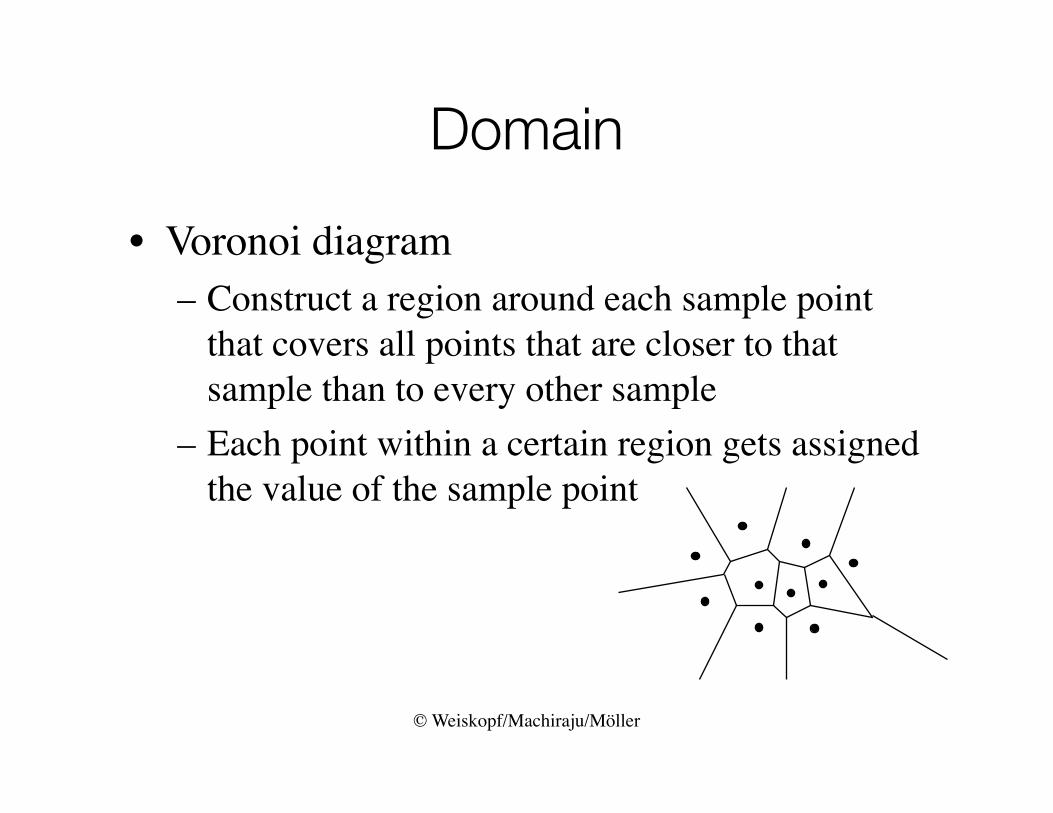
Domain
• Voronoi diagram– Construct a region around each sample point
that covers all points that are closer to that sample than to every other sample
– Each point within a certain region gets assigned the value of the sample point
© Weiskopf/Machiraju/Möller
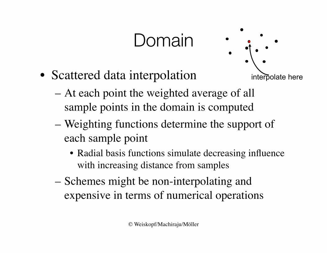
Domain
• Scattered data interpolation– At each point the weighted average of all
sample points in the domain is computed– Weighting functions determine the support of
each sample point• Radial basis functions simulate decreasing influence
with increasing distance from samples– Schemes might be non-interpolating and
expensive in terms of numerical operations
interpolate here
© Weiskopf/Machiraju/Möller
Data Structures
• Requirements:– Efficiency of accessing data– Space efficiency– Lossless vs. lossy – Portability
• Binary – less portable, more space/time efficient• Text – human readable, portable, less space/time efficient
• Definition – If points are arbitrarily distributed and no connectivity
exists between them, the data is called scattered– Otherwise, the data is composed of cells bounded by grid
lines– Topology specifies the structure (connectivity) of the data – Geometry specifies the position of the data
© Weiskopf/Machiraju/Möller
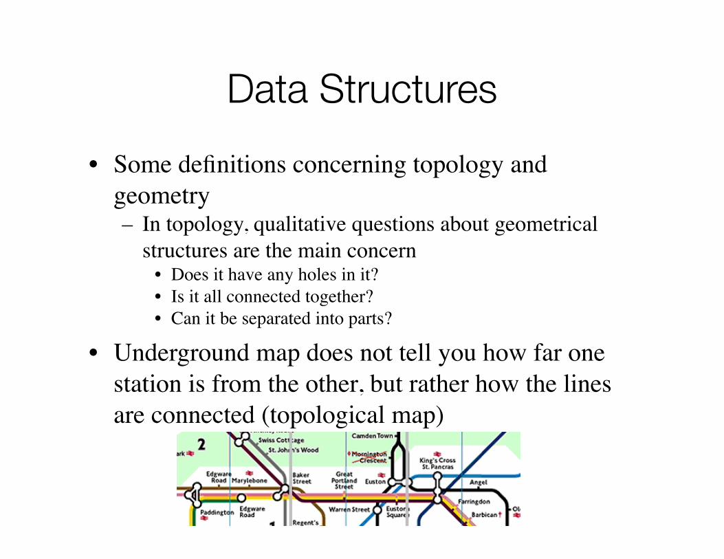
Data Structures
• Some definitions concerning topology and geometry– In topology, qualitative questions about geometrical
structures are the main concern • Does it have any holes in it?• Is it all connected together?• Can it be separated into parts?
• Underground map does not tell you how far one station is from the other, but rather how the lines are connected (topological map)

© Weiskopf/Machiraju/Möller
Data Structures
• Topology– Properties of geometric shapes that remain
unchanged even when under distortion
Same geometry (vertex positions), different topology (connectivity)
© Weiskopf/Machiraju/Möller
Data Structures
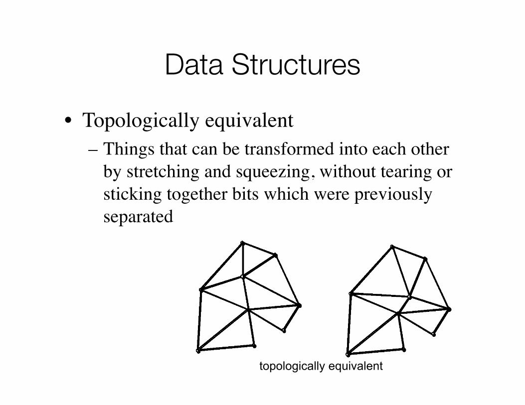
• Topologically equivalent– Things that can be transformed into each other
by stretching and squeezing, without tearing or sticking together bits which were previously separated
topologically equivalent
© Weiskopf/Machiraju/Möller
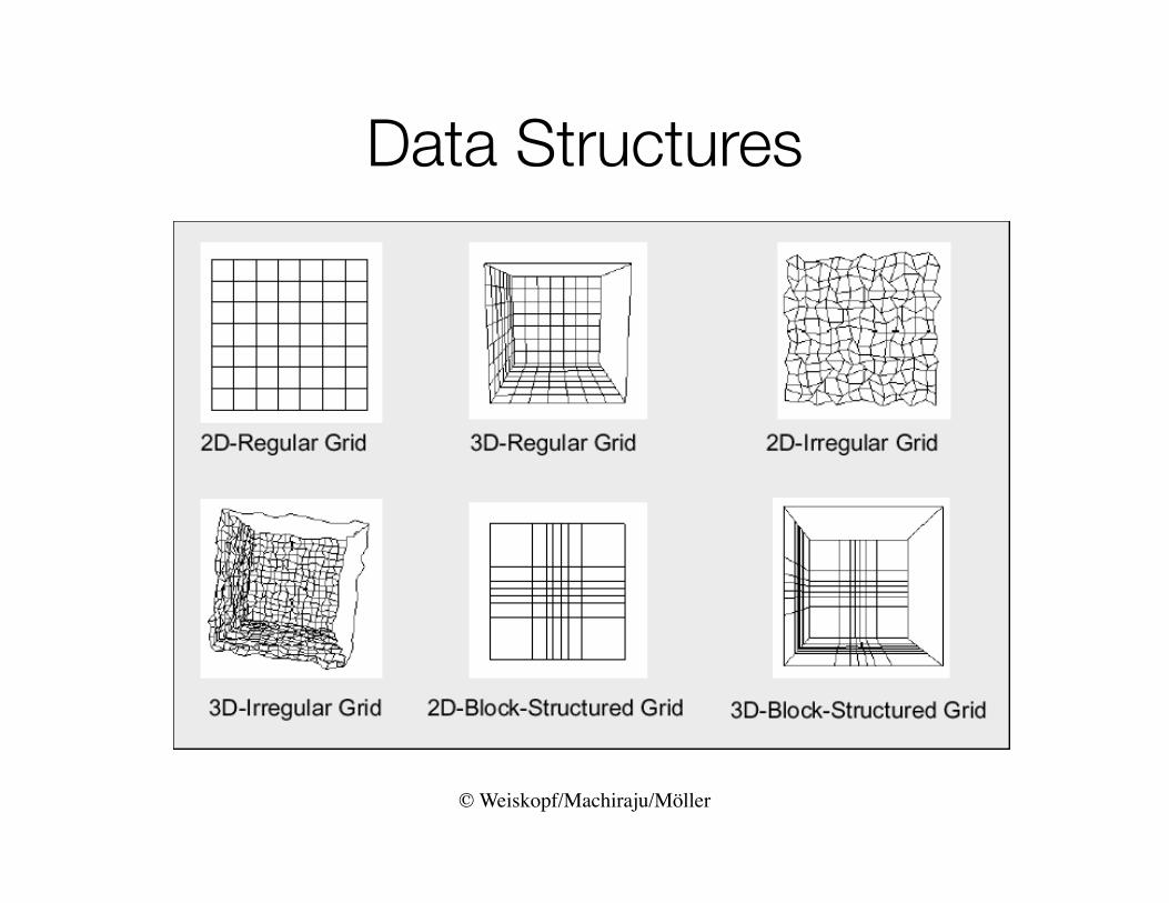
Data Structures
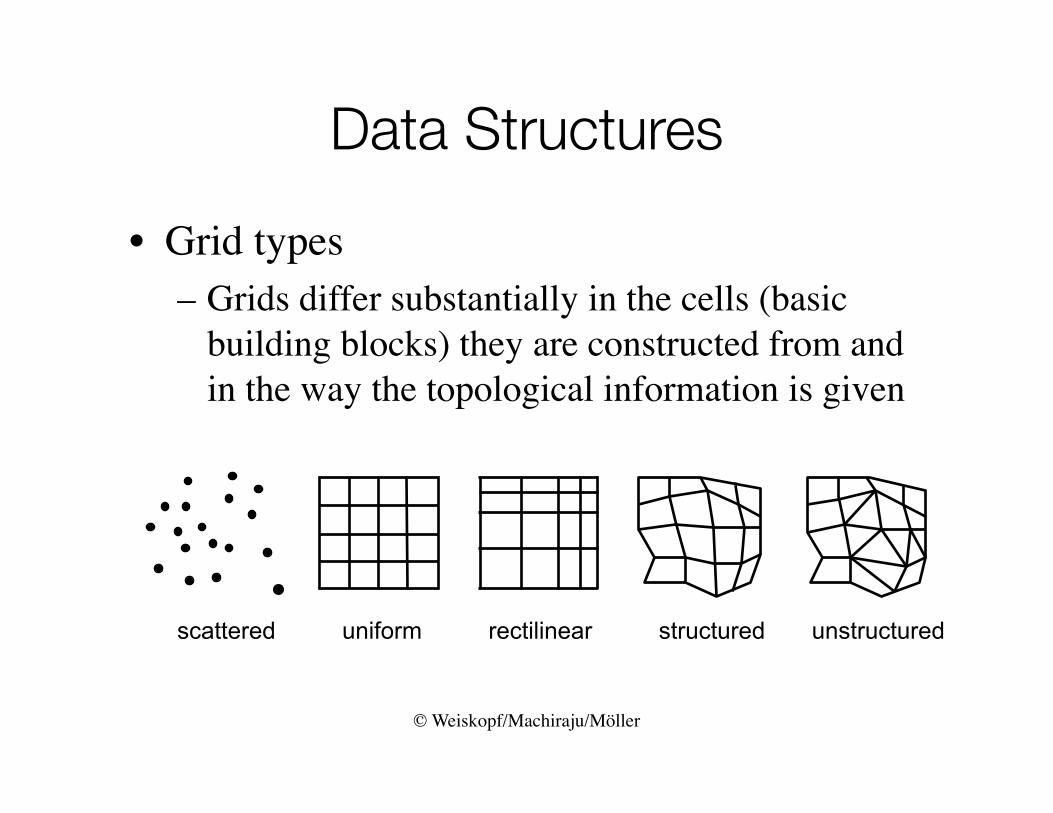
• Grid types– Grids differ substantially in the cells (basic
building blocks) they are constructed from and in the way the topological information is given
scattered uniform rectilinear structured unstructured
© Weiskopf/Machiraju/Möller
Data Structures
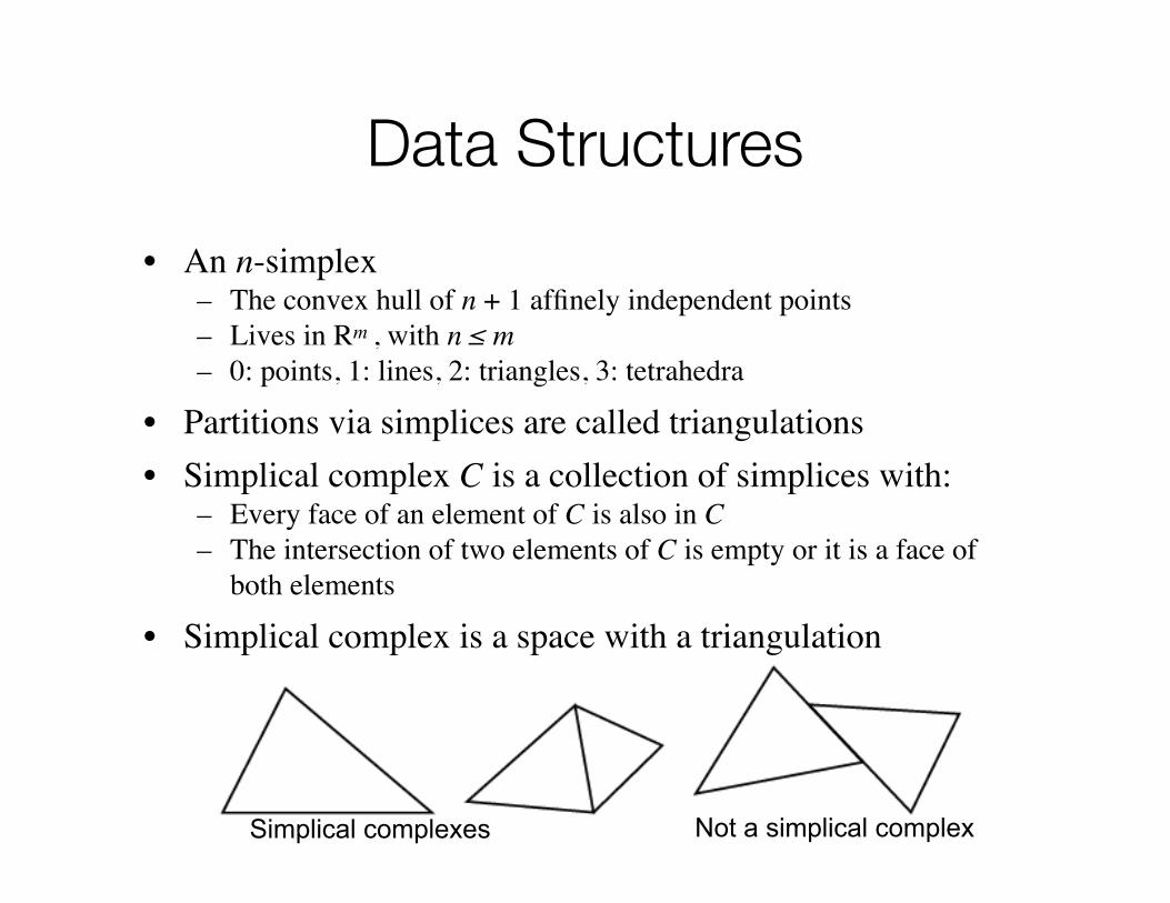
• An n-simplex– The convex hull of n + 1 affinely independent points– Lives in Rm , with n ≤ m – 0: points, 1: lines, 2: triangles, 3: tetrahedra
• Partitions via simplices are called triangulations• Simplical complex C is a collection of simplices with:
– Every face of an element of C is also in C– The intersection of two elements of C is empty or it is a face of
both elements
• Simplical complex is a space with a triangulation
Simplical complexes Not a simplical complex
© Weiskopf/Machiraju/Möller
Data Structures
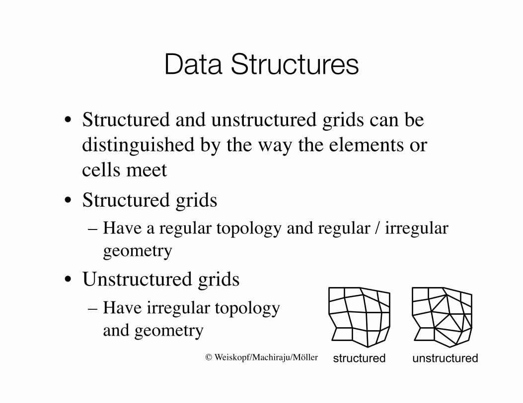
• Structured and unstructured grids can be distinguished by the way the elements or cells meet
• Structured grids – Have a regular topology and regular / irregular
geometry• Unstructured grids
– Have irregular topology and geometry
structured unstructured
© Weiskopf/Machiraju/Möller
Data Structures
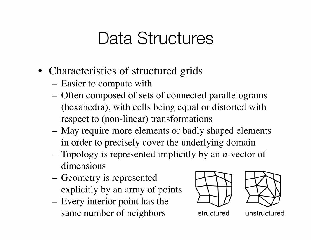
• Characteristics of structured grids– Easier to compute with– Often composed of sets of connected parallelograms
(hexahedra), with cells being equal or distorted with respect to (non-linear) transformations
– May require more elements or badly shaped elements in order to precisely cover the underlying domain
– Topology is represented implicitly by an n-vector of dimensions
– Geometry is represented explicitly by an array of points
– Every interior point has the same number of neighbors structured unstructured
© Weiskopf/Machiraju/Möller
Data Structures
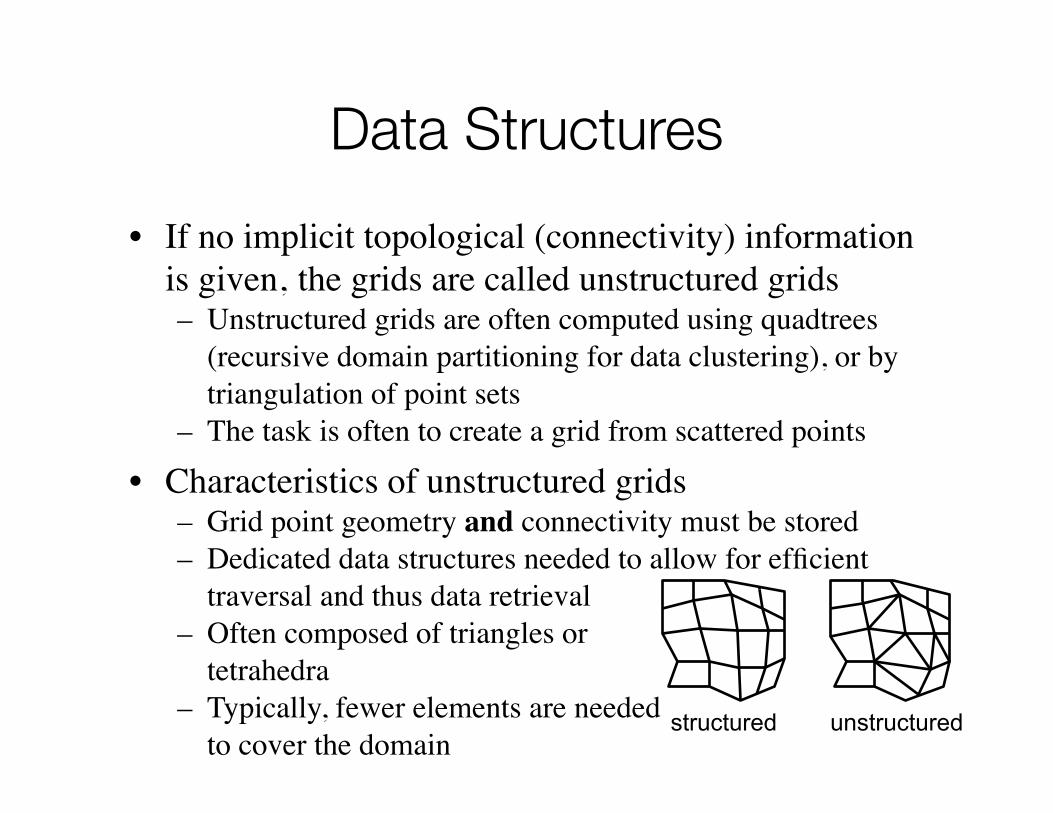
• If no implicit topological (connectivity) information is given, the grids are called unstructured grids– Unstructured grids are often computed using quadtrees
(recursive domain partitioning for data clustering), or by triangulation of point sets
– The task is often to create a grid from scattered points
• Characteristics of unstructured grids– Grid point geometry and connectivity must be stored– Dedicated data structures needed to allow for efficient
traversal and thus data retrieval– Often composed of triangles or
tetrahedra– Typically, fewer elements are needed
to cover the domainstructured unstructured
© Weiskopf/Machiraju/Möller
Data Structures
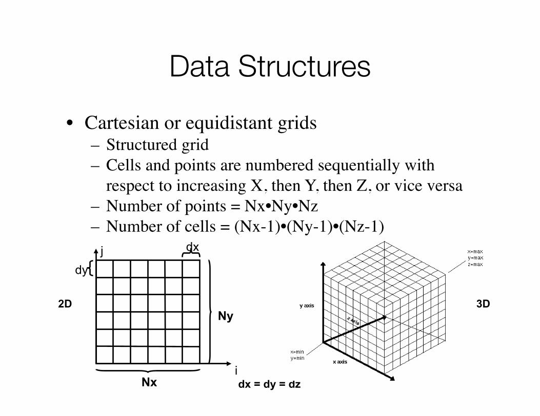
• Cartesian or equidistant grids– Structured grid– Cells and points are numbered sequentially with
respect to increasing X, then Y, then Z, or vice versa– Number of points = Nx•Ny•Nz– Number of cells = (Nx-1)•(Ny-1)•(Nz-1)
dx = dy = dz
2D 3DNy
iNx
j dx
dy
© Weiskopf/Machiraju/Möller
Data Structures
• Cartesian grids– Vertex positions are given implicitly from [i,j,k]:
• P[i,j,k].x = origin_x + i • dx• P[i,j,k].y = origin_y + j • dy• P[i,j,k].z = origin_z + k • dz
– Global vertex index I[i,j,k] = k•Ny•Nx + j•Nx + i• k = I / (Ny•Nx)• j = (I % (Ny•Nx)) / Nx• i = (I % (Ny•Nx)) % Nx
– Global index allows for linear storage scheme• Wrong access pattern might destroy cache coherence
© Weiskopf/Machiraju/Möller
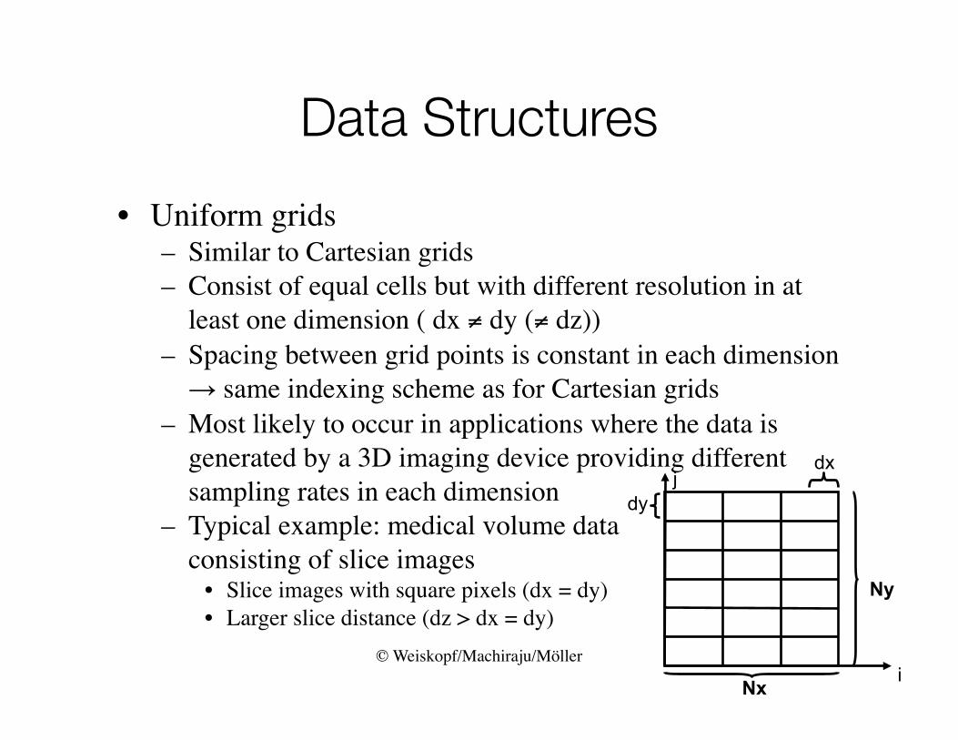
Data Structures
• Uniform grids– Similar to Cartesian grids– Consist of equal cells but with different resolution in at
least one dimension ( dx ≠ dy (≠ dz))– Spacing between grid points is constant in each dimension→ same indexing scheme as for Cartesian grids
– Most likely to occur in applications where the data is generated by a 3D imaging device providing different sampling rates in each dimension
– Typical example: medical volume data consisting of slice images
• Slice images with square pixels (dx = dy) • Larger slice distance (dz > dx = dy)
Nx
Ny
i
jdx
dy
© Weiskopf/Machiraju/Möller
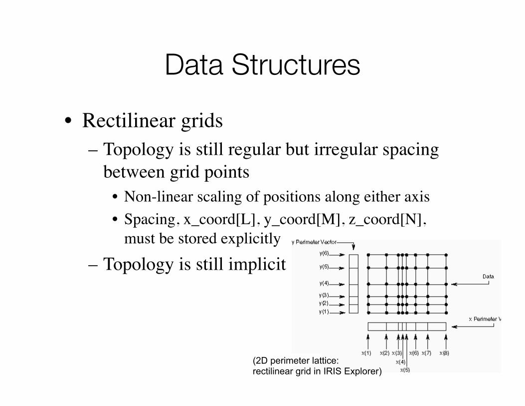
Data Structures
• Rectilinear grids– Topology is still regular but irregular spacing
between grid points • Non-linear scaling of positions along either axis• Spacing, x_coord[L], y_coord[M], z_coord[N],
must be stored explicitly– Topology is still implicit
(2D perimeter lattice:rectilinear grid in IRIS Explorer)
© Weiskopf/Machiraju/Möller
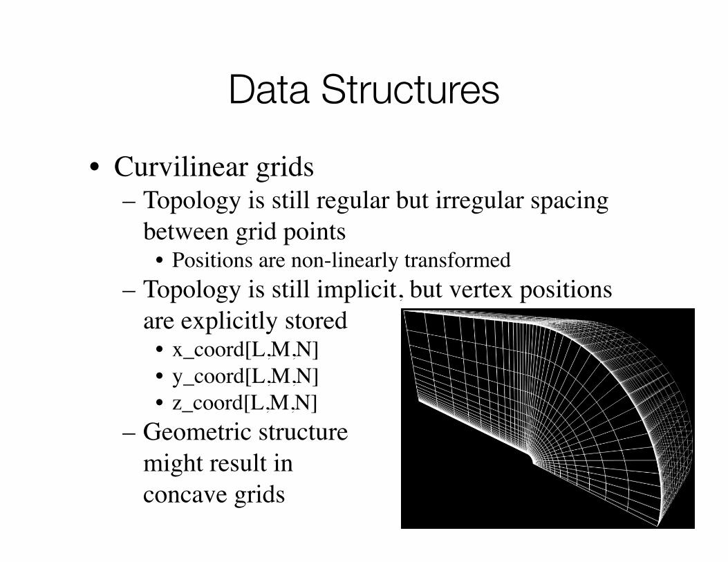
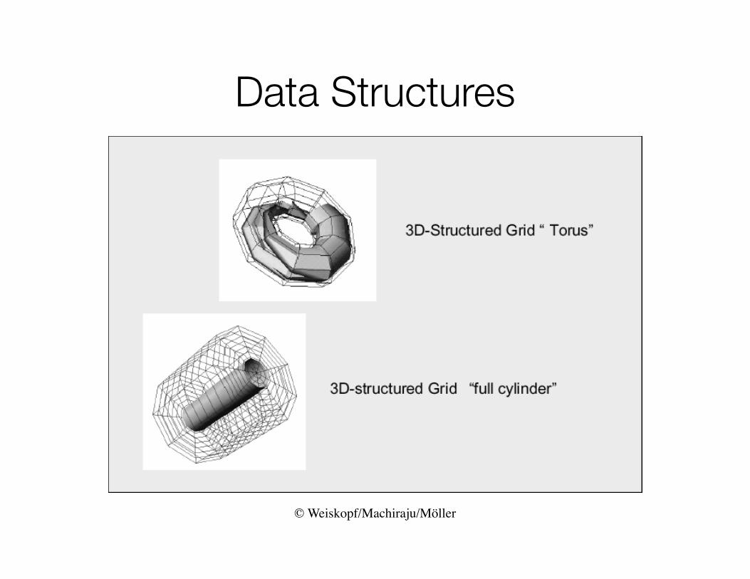
Data Structures
• Curvilinear grids– Topology is still regular but irregular spacing
between grid points• Positions are non-linearly transformed
– Topology is still implicit, but vertex positions are explicitly stored
• x_coord[L,M,N]• y_coord[L,M,N]• z_coord[L,M,N]
– Geometric structure might result in concave grids
© Weiskopf/Machiraju/Möller
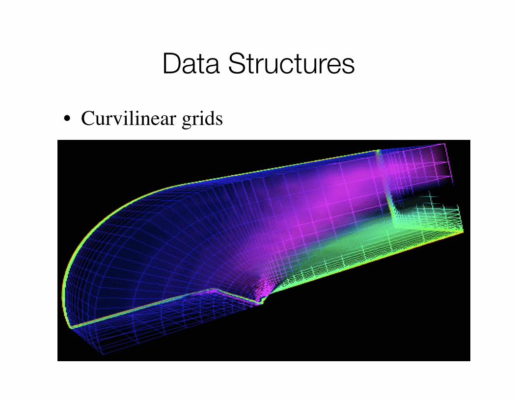
Data Structures
• Curvilinear grids
© Weiskopf/Machiraju/Möller
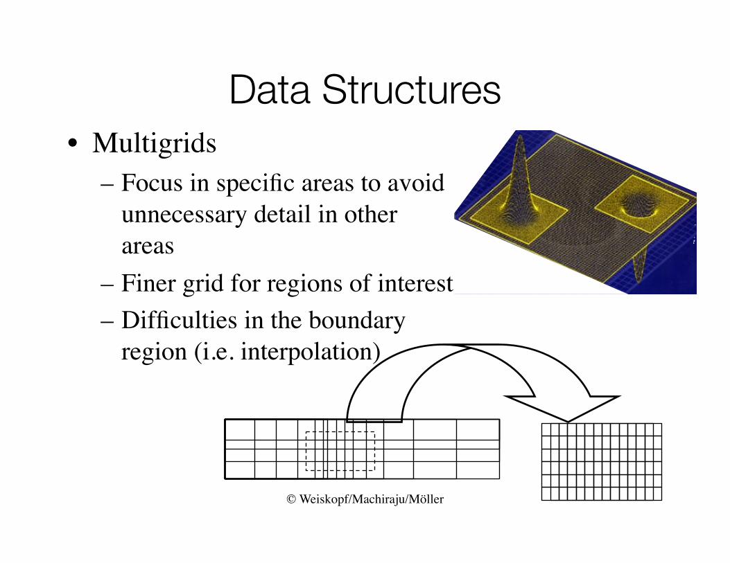
Data Structures• Multigrids
– Focus in specific areas to avoid unnecessary detail in other areas
– Finer grid for regions of interest– Difficulties in the boundary
region (i.e. interpolation)
© Weiskopf/Machiraju/Möller
Data Structures
• Characteristics of structured grids– Structured grids can be stored in a 2D / 3D array– Arbitrary samples can be directly accessed by indexing a
particular entry in the array– Topological information is implicitly coded
• Direct access to adjacent elements– Cartesian, uniform, and rectilinear grids are necessarily convex– Their visibility ordering of elements with respect to any
viewing direction is given implicitly– Their rigid layout prohibits the geometric structure to adapt to
local features– Curvilinear grids reveal a much more flexible alternative to
model arbitrarily shaped objects– However, this flexibility in the design of the geometric shape
makes the sorting of grid elements a more complex procedure
© Weiskopf/Machiraju/Möller
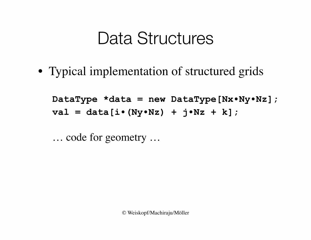
Data Structures
• Typical implementation of structured grids
DataType *data = new DataType[Nx•Ny•Nz];val = data[i•(Ny•Nz) + j•Nz + k];
… code for geometry …
© Weiskopf/Machiraju/Möller
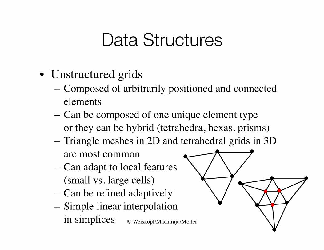
Data Structures
• Unstructured grids – Composed of arbitrarily positioned and connected
elements– Can be composed of one unique element type
or they can be hybrid (tetrahedra, hexas, prisms)– Triangle meshes in 2D and tetrahedral grids in 3D
are most common– Can adapt to local features
(small vs. large cells)– Can be refined adaptively– Simple linear interpolation
in simplices
© Weiskopf/Machiraju/Möller
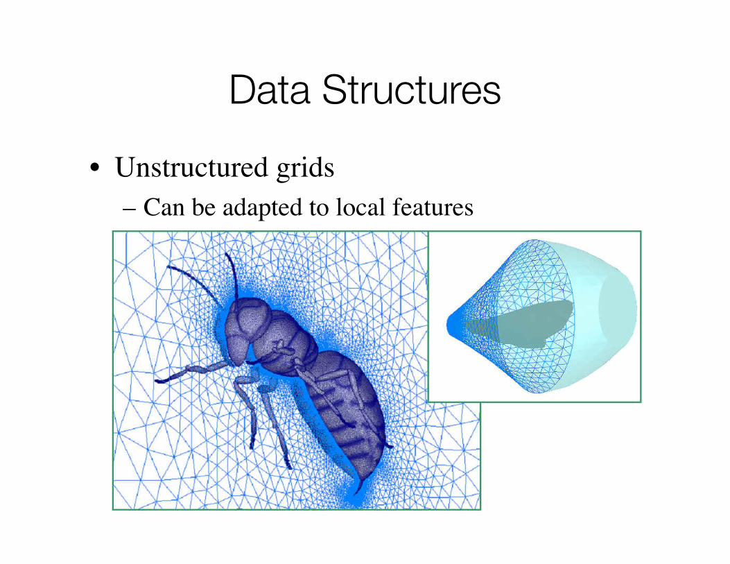
Data Structures
• Unstructured grids – Can be adapted to local features
© Weiskopf/Machiraju/Möller
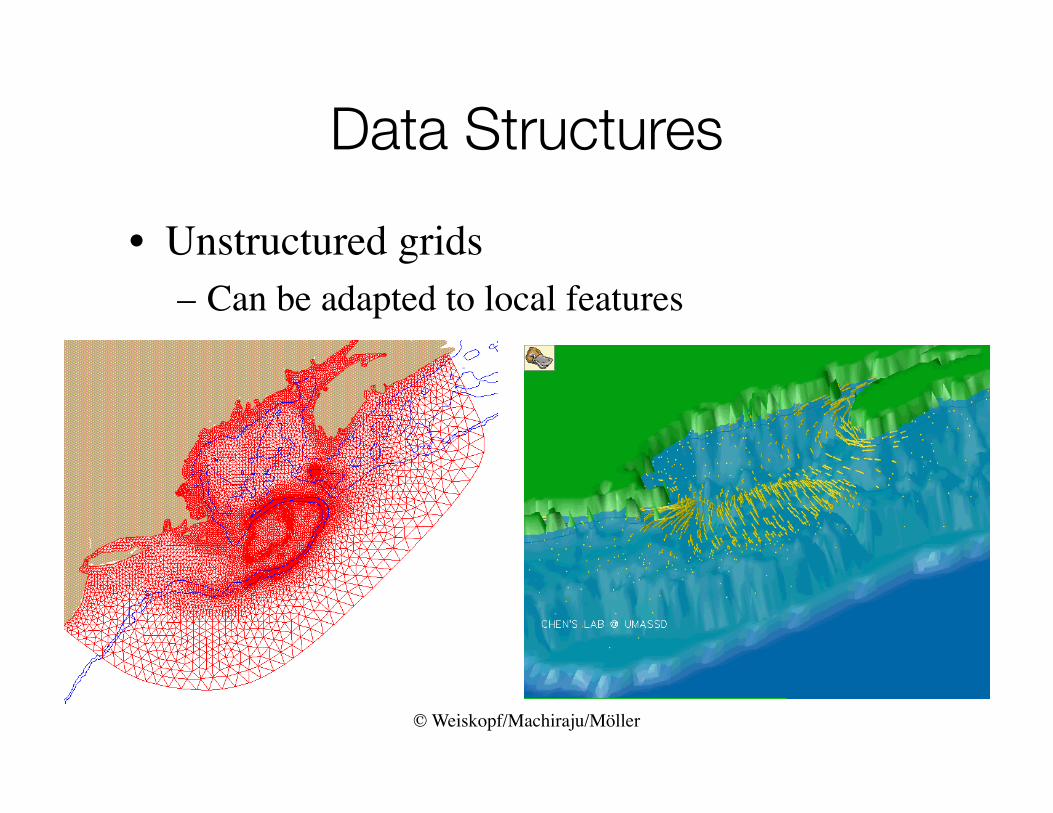
Data Structures
• Unstructured grids – Can be adapted to local features
© Weiskopf/Machiraju/Möller
Data Structures
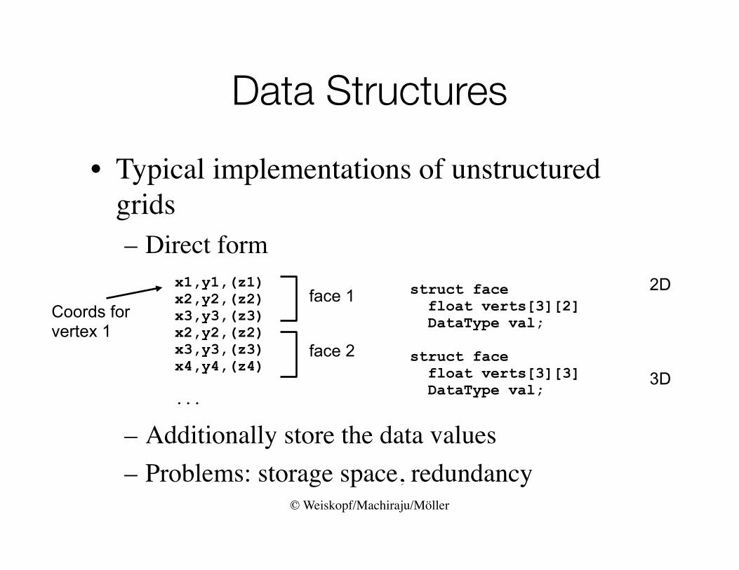
• Typical implementations of unstructured grids– Direct form
– Additionally store the data values– Problems: storage space, redundancy
struct face float verts[3][2] DataType val;
struct face float verts[3][3] DataType val;
x1,y1,(z1) x2,y2,(z2)x3,y3,(z3)x2,y2,(z2) x3,y3,(z3)x4,y4,(z4)
...
face 1
face 2
2D
3D
Coords for vertex 1
© Weiskopf/Machiraju/Möller
Data Structures
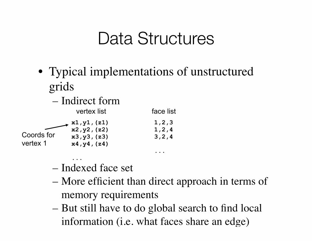
• Typical implementations of unstructured grids– Indirect form
– Indexed face set– More efficient than direct approach in terms of
memory requirements– But still have to do global search to find local
information (i.e. what faces share an edge)
x1,y1,(z1) x2,y2,(z2)x3,y3,(z3)x4,y4,(z4)
...
vertex list face list1,2,3 1,2,43,2,4
...
Coords for vertex 1
© Weiskopf/Machiraju/Möller
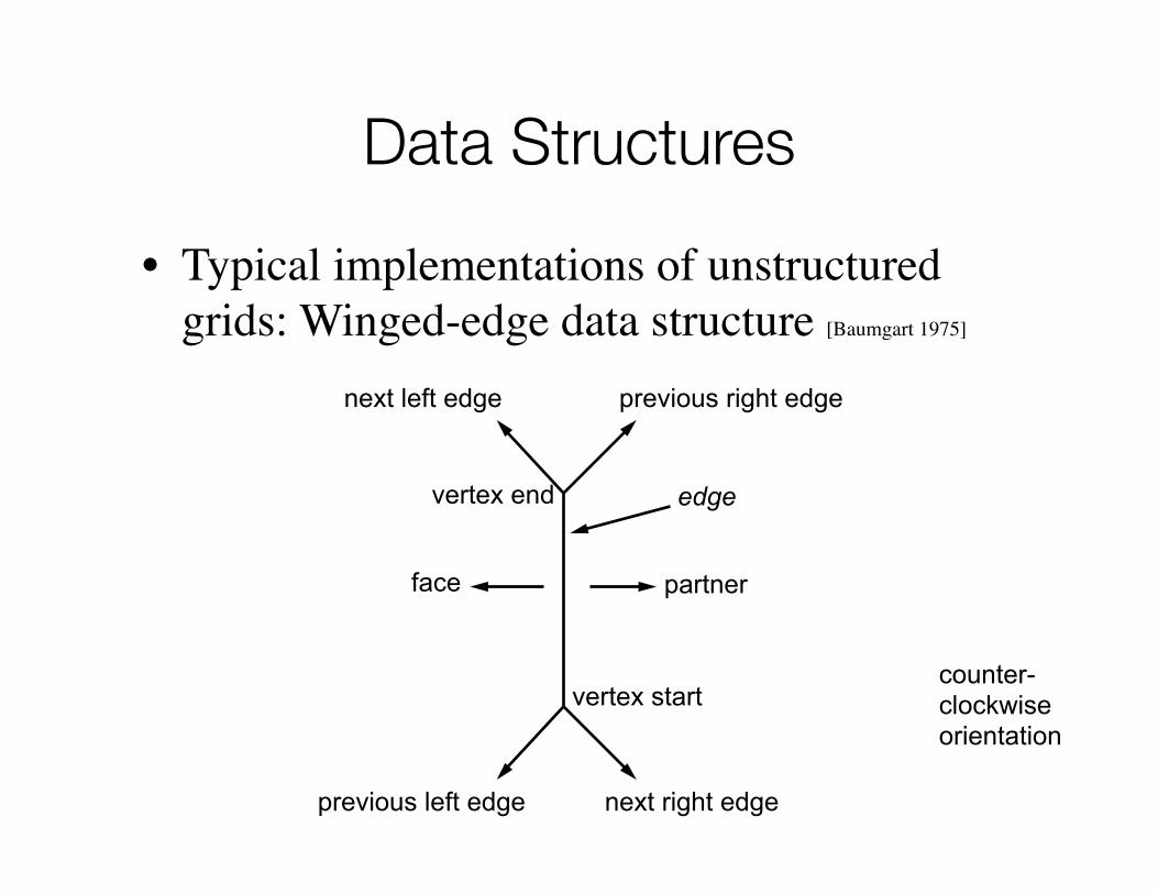
Data Structures
• Typical implementations of unstructured grids: Winged-edge data structure [Baumgart 1975]
next left edge previous right edge
edge
face partner
previous left edge next right edge
vertex start
vertex end
counter-clockwiseorientation
© Weiskopf/Machiraju/Möller
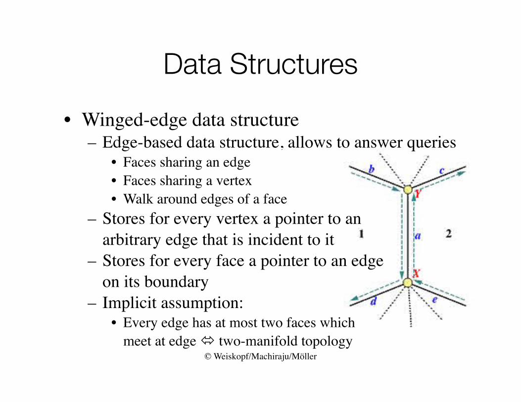
Data Structures
• Winged-edge data structure– Edge-based data structure, allows to answer queries
• Faces sharing an edge• Faces sharing a vertex• Walk around edges of a face
– Stores for every vertex a pointer to anarbitrary edge that is incident to it
– Stores for every face a pointer to an edgeon its boundary
– Implicit assumption:• Every edge has at most two faces which
meet at edge two-manifold topology
© Weiskopf/Machiraju/Möller
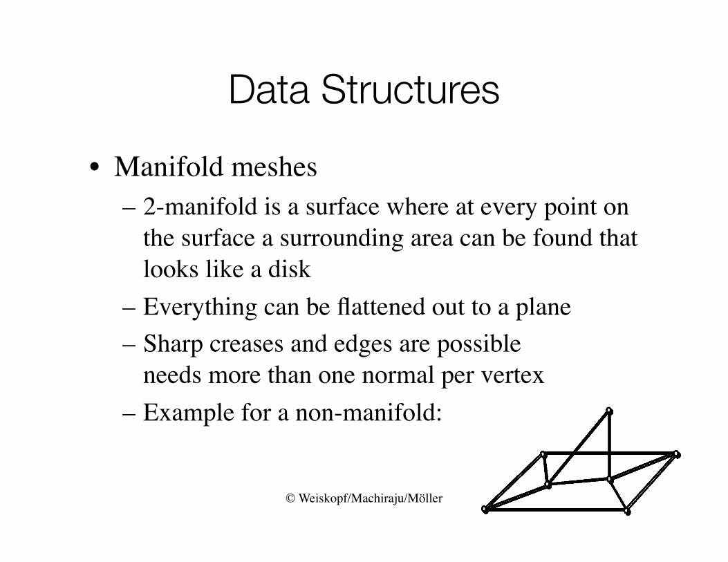
Data Structures
• Manifold meshes– 2-manifold is a surface where at every point on
the surface a surrounding area can be found that looks like a disk
– Everything can be flattened out to a plane– Sharp creases and edges are possible
needs more than one normal per vertex– Example for a non-manifold:
© Weiskopf/Machiraju/Möller
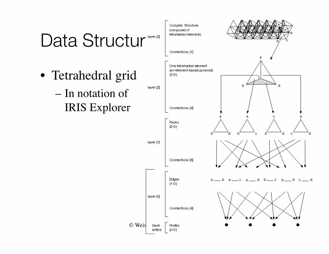
Data Structures
• Tetrahedral grid– In notation of
IRIS Explorer
© Weiskopf/Machiraju/Möller
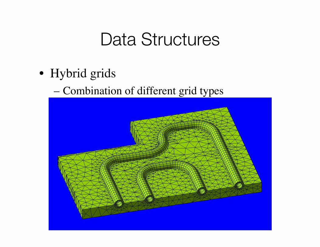
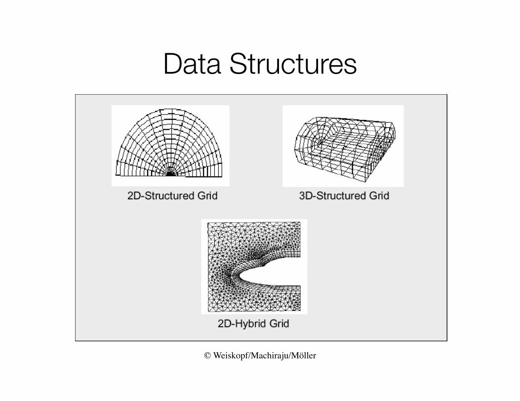
Data Structures
• Hybrid grids– Combination of different grid types
© Weiskopf/Machiraju/Möller
Data Structures
© Weiskopf/Machiraju/Möller
Data Structures
© Weiskopf/Machiraju/Möller
Data Structures
© Weiskopf/Machiraju/Möller
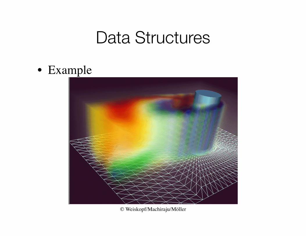
Data Structures
• Example
© Weiskopf/Machiraju/Möller
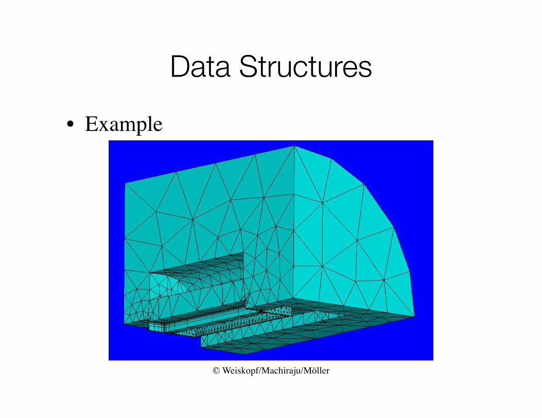
Data Structures
• Example
© Weiskopf/Machiraju/Möller
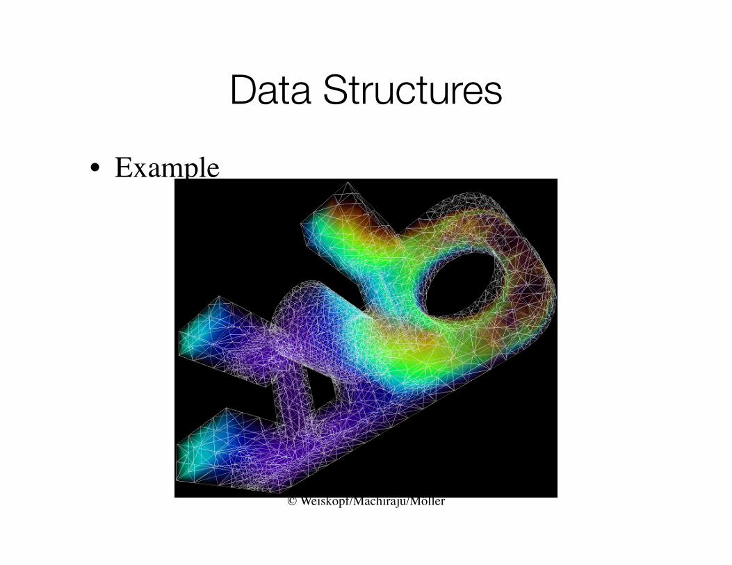
Data Structures
• Example
© Weiskopf/Machiraju/Möller
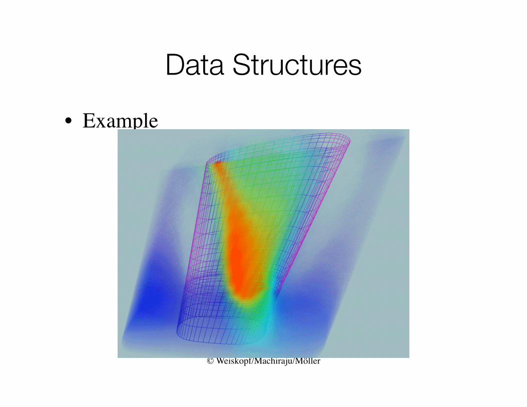
Data Structures
• Example
© Weiskopf/Machiraju/Möller
Data Structures
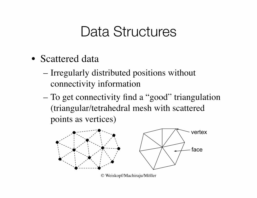
• Scattered data– Irregularly distributed positions without
connectivity information– To get connectivity find a “good” triangulation
(triangular/tetrahedral mesh with scattered points as vertices)
vertex
face
© Weiskopf/Machiraju/Möller
Data Structures
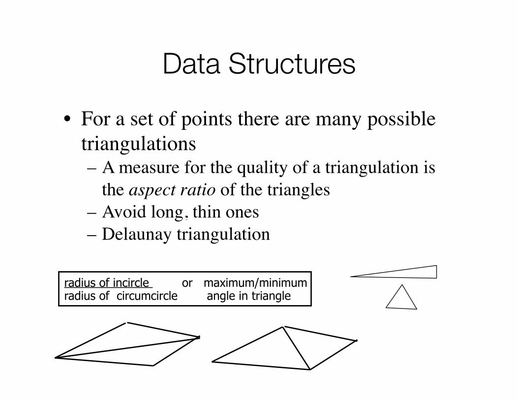
• For a set of points there are many possible triangulations– A measure for the quality of a triangulation is
the aspect ratio of the triangles– Avoid long, thin ones– Delaunay triangulation
radius of incircle or maximum/minimumradius of circumcircle angle in triangle