04 5 SummingBellStirling - Index Homepage Gottfried · PDF fileAlternating sums of Bell- and Stirling-numbers S. -2- Identities with binomials,Bernoulli- and other numbertheoretical

Identities involving binomial-coefficients,

Bernoulli- and Stirlingnumbers

Gottfried Helms - Univ Kassel since 12 - 2006

Bell-Numbers

Alternating sums of Bell-numbers and of Stirling-numbers 2nd kind

Abstract: This article has two motivations:

an exercise in translation of another number-theoretical aspect into my

matrix-concept

and -following from this- an approach to a special matrix-based summa-

tion-method using a concrete example.

I consider the definition of Bell-numbers based on the article of E.T. Bell

(1938). The matrix approach shows a very elegant and concise notion of

those Bell-numbers and their higher (integer) orders, and finally of their

generalization to fractional/ continuous orders which can be described

very concisely using the matrix-logarithm.

Derived from that I show an approach to sum the alternating series of

Bell-numbers. This series is strongly divergent, so that Euler-summation

is not sufficient to assign a value to it. The result of this is compared

with a serial summation using the idea of the Riesz-method (see:

[Knopp]). An implicite effect is a summation-concept for the alternating

sums of columns of the matrix of Stirling-numbers 2nd kind (again diver-

gent, but can be Euler-summed); this result, however, is already known.

The derivations given here use the concept of matrix-operators, acting

on formal powerseries. I'd like to promote this concept due to its concise

and versatile notation, although it lacks widely formal proofs. I'm trying

to collect a compilation of basic proofs independent of this series of arti-

cles.

For more basic and general introduction see "intro"1 of my "binomial-

matrices"-project.

Gottfried Helms, 04.07.08 Version 3.2

Contents

1. Definition of Bell-numbers.............................................................................................................2

1.1. Definition ............................................................................................................................2

1.2. Relation to the matrix S2 of Stirling-numbers 2nd kind. .....................................................2

1.3. Iteration ...............................................................................................................................5

1.4. some recursive properties ....................................................................................................6

1.5. Generalization to fractional (and complex) orders m ..........................................................7

1.6. Short Summary....................................................................................................................8

1.7. Conclusion...........................................................................................................................9

2. Further interesting properties of the Bell/Stirling-numbers.........................................................10

2.1. Alternating sums of Bell-numbers.....................................................................................10

2.2. Alternating sum of B(2)-numbers .......................................................................................16

2.3. Alternating sum of B(m) of same index ..............................................................................18

3. Appendix ......................................................................................................................................20

3.1. Proof: Binomial sum of reciprocals ...................................................................................20

4. References ....................................................................................................................................21

1 Intro/notation http://go.helms-net.de/math/binomial/intro.pdf

MathematMathematMathematMathematiiiicalcalcalcal

MiniaturesMiniaturesMiniaturesMiniatures

Alternating sums of Bell- and Stirling-numbers S. -2-

Identities with binomials,Bernoulli- and other numbertheoretical numbers Mathematical Miniatures

1. Definition of Bell-numbers

1.1. Definition

The concept of the "Bell"-numbers was developed by E. T. Bell around

1938; I refer here to the article "Iterate exponential integers" [Bell38],

where he used the name "ξ-number" for his integers. He derived the ξ-

numbers initially using exp(exp(x)-1) as exponential generation function

("e.g.f."). Then he introduces iteration, defining the inner function E(1) =

exp(1)-1 and its iterates E(m+1)=exp(E(m))-1 and generalizes the ξ-numbers to

ξ(m)-numbers using the m'th iterate in the expression exp(E(m)) as e.g.f. for

ξ(m)

From this, the infinite sequences ξ(m) of order m are defined

ξ(m) =sequencen=0..inf ( ξ(m)

n ) generated by e.g.f exp(E(m))

ξ(0) =sequencen=0..inf ( ξ(m)

n ) ; e.g.f exp(E(0)) = exp(1)

The sequences ξ(m) for consecutive m can be written as matrix of infinite

size ξ, where the m'th column contains the m'th sequence (the matrix-

indices begin at zero as well), so column 0 contains all 1, and column 1 con-

tains ξ(1)n = (1,1,2,5,...)

ξ =

1.2. Relation to the matrix S2 of Stirling-numbers 2nd kind.

Using the function E(1) = exp(x)-1 as e.g.f gives the second column of the

matrix of Stirling-numbers 2nd kind as coefficients. This matrix begins

S2 =

(infinitely continued)

Using exp(E(1)) as e.g.f for its formal parameter E(1), we get the sequence

(1,1,1,..) as cofactors for the powers (E(1))0, (E(1))1 ,(E(1))2, ...); expanding

these powers into series in x and collecting like powers of x gives then the

intended coefficients ξ(1)n = (1,1,2,5,...) as cofactors at x0, x1, x2, ...



Now, the c'th column of S2S2S2S2 contains just the required coefficients for the

powers (E(1))c (as for instance given in [A&S],pg. 824), such that

Xf~ * S2 = Yf~

Example:

Xf~ * S2 = Yf~

*

=

where y is y=E(1)=exp(x)-1. The small f at Xf and Yf indicate the scaling of

the X and the Y-vector by the reciprocal factorials and the ~-symbol the

transposition of a matrix/vector (see below).

Repeat: while the coefficents at consecutive powers of y are (1,1,1,1,..) if

we use the e.g.f exp(y), the ξ(1)-numbers are defined by the e.g.f.

of exp(exp(x)-1) as the coefficients of powers of x.

The coefficients ξ(1)=sequence(ξ(1)0,ξ

(1)1,ξ

(1)2,...) are found after yk

are expanded into powers of x and like powers of x are collected.

Such an expansion is tedious when done sequentially, but is easy when

written in matrix-notation.

Some helpful notational definitions

To express this all in a more consistent form than that of the above ad-hoc

matrix-sketch I first want to introduce few formalisms to get consistency with

the general style of my matrix-formulae around.

All vectors and matrices are assumed with infinite size.

define

V(x) :=columnvector(1,x,x2,x3,...)

to be a formal "vandermonde vector" of a free parameter x

dV(x) :=diag(1,x,x2,x3,...)

using V(x) as a diagonal-matrix

define

F :=columnvector(0!,1!,2!,3!,...)

dF := diag(0!,1!,2!,3!,...)

define the diagonal-matrix for shortness in matrix-formulae

J:= Jk,k= (-1)k

so J = dV(-1)

define "~" being the "transpose"-symbol

(as used in the algebra-program Pari/GP)

Sometimes I also use the abbreviation for a similarity-scaling

fS2F = dF-1 * S2 * dF

to keep matrix-expressions simpler in notation.



With this, the e.g.f-relation of exp(y) and the according coefficients may be

written as

Yf~ * V(1) = exp(y)

Example:

Yf~ * V(1) = exp(y)

*

= exp(y)

But YfYfYfYf is also composed by

Xf~ *S2 = Yf~

Example:

Xf~ *S2 = Yf~

*

=

as shown above.

So the full matrix-equation is

Xf ~ *S2 *V(1) = exp(exp(x)-1)

Example:

Xf ~ *S2 *V(1) = exp(exp(x)-1)

* *

= exp(exp(x)-1)

To get the coefficients at the powers of x, we reorder the summation in the

formula

exp(exp(x)-1) = Xf~ * S2 *V(1)

= Xf~ *(S2 *V(1))

= Xf~ * ξ(1)

⇒⇒⇒⇒ ξ(1) = S2 *V(1)

where the numbers ξ(1)n occur simply as rowsums of the S2S2S2S2-matrix and we

have the definition of ξ(1) by the Stirling-numbers 2nd kind:

S2 * V(1) = ξ (1)



Example:

S2 * V(1) = ξ(1)

*

=

and then

Xf ~ * ξ(1) = exp(exp(x)-1)

Example:

Xf ~ * ξ(1) = exp(exp(x)-1)

*

= exp(exp(x)-1)

1.3. Iteration

The ξ(2) coefficients are found by the e.g.f. for

exp(z) = exp(exp(y)-1) = exp(exp(exp(x)-1)-1)

the same way just by iteration, where y takes the place of the previous x

and z takes the place of the previous y:

Zf~ = Yf~* S2

= Xf~* S2 * S2

= Xf~* S22

exp( exp(exp(x)-1)-1) = Xf~ * S22 *V(1)

= Xf~ * ξ(2)

⇒⇒⇒⇒ ξ(2) = S22 *V(1)

where the numbers ξ(2)n occur as rowsums of S2 S2 S2 S2 2.

S22 * V(1) = ξ(2)

Example:

S22 * V(1) = ξ(2)

*

=



and then

Xf ~ * ξ(2) = exp(exp(exp(x)-1) –1)

Example:

Xf ~ * ξ(2) = exp(exp(exp(x)-1) –1)

*

= exp(exp(exp(x)-1)-1)

Obviously this can be generalized to any integer index m:

ξ(m) = S2 m * V(1)

1.4. some recursive properties

From the simple matrix-relation also some simple recursion-schemes can be

derived:

ξ(0) = V(1)

ξ(m) = S2 * ξ(m-1)

ξ(m) = S2-1 * ξ(m+1) = S1 * ξ(m+1) // S1: Stirling-numbers of 1st kind

This says, in scalar expression

( ) ( )∑∑=

+

=

− ==r

0c

)1m(

cc,r

r

0c

)1m(

cc,r

)m(

r 1S2S ξξξ

where S2S2S2S2r,c are the Stirling-numbers 2nd kind and S1S1S1S1r,c that of the 1st kind,

at row r and col c of the resp. triangle.

Also, since the premultiplication with the Pascal-/Binomialmatrix PPPP the ma-

trix S2S2S2S2 is shifted by one row/column, we get a shifting of the index for the

ξ(1) –numbers if they are binomially summed; the ξ(1)-number ξ(1)r+1 can be

computed by the binomially weighted previous ones, which can also be used

as a recursive definition:

ξ(1)r+1 = ∑

=

r

0k

)1(

kk

rξ

Example:

ξ(1)r+1 = ∑

=

r

0k

)1(

kk

rξ

* ⇒

= ⇒



Arbitrarily we may find more of such relations and recursive (re-) defini-

tions, whose general numbertheoretical importance, however, must be

shown.

1.5. Generalization to fractional (and complex) orders m

Fractional orders m can be defined in the obvious way: by finding an inter-

polation-formula for each r'th row of the list of ξ(m) , so interpolate(ξ(0)r, ξ

(1)r,

ξ(2)r, ... ξ

(m)r,...) gives polynomials in m, for which then fractional (or even

complex) orders can be defined. E.T. Bell gives the first few such polynomi-

als as

ξ(m)1 = 1

ξ(m)2 = m + 1

ξ(m)3 = 1/2(m + 1)(3m+2)

ξ(m)4 = 1/2(m + 1)(2m+1)(3m+2)

ξ(m)5 = 1/6(m + 1)(45m3 + 70m2 +35m+6)

(...)

and derives these formulae by considering the differences ξ(m+1)r - ξ

(m)r and

expanding into polynomials.

Using the matrix-notation, we may refer to the formula

ξ(m) = S2 m * V(1)

and ask for the fractional m'th power of S2S2S2S2, where I now use "s" for the

fractional or complex generalization of m.

The most simple approach is to use the matrix-logarithm and restate:

ξ(s) = exp(s*log(S2)) * V(1)

Since the diagonal of S2S2S2S2 contains only the unit, the matrix (S2S2S2S2 – I I I I ), which is

needed for the computation of log(S2S2S2S2) by the powerseries expansion of the

log-function, is nilpotent for each number of rows/columns considered and

so the logarithm-function reduces –for any finite approximation - to a finite

sum of scaled powers of (S2 (S2 (S2 (S2 –––– I ) I ) I ) I ). Increasing the size does not affect the coef-

ficients, so any top-left segment found by this is exact in rational arithmetic.

The matrix-logarithm S2LS2LS2LS2L = log(S2S2S2S2) has its top-left segment as

S2L = log(S2) =

Then we can find the symbolic description of the s'th power S2 S2 S2 S2 2 by matrix-

exponentiation S2S2S2S2 s = exp(s*S2LS2LS2LS2L):

Example:

S2s = exp(s*S2L) =

whose top-left segment is again exact for any size of the matrix (by the

same arguments as above).



The fractional s'th order of the ξ-numbers are given by the rowsums:

ξ(s) = S2 s * V(1)

Example:

ξ(s) = S2 s * V(1)

(where we find ξ(s)n if we evaluate the n'th row) which is the same as the

solution given by E.T. Bell using the interpolation formula.

1.6. Short Summary

The above matrix-notation gives some concise formulae for the ξ –numbers.

definition by translation into matrix-language:

ξ(m) = S2 m * V(1)

recursion over orders

ξ(0) = V(1)

ξ(m+1) = S2 * ξ(m)

ξ(m-1) = S1 * ξ(m) // not seen before

recursion by index shift

shift(ξ(1) ) = P * ξ(1) // computes ξ(1) n+1 from ξ(1)0 ...ξ

(1)n

fractional / general orders

ξ(s) = exp(s*log(S2)) * V(1)

alternating sums of ξ(1) and ξ(2) (see next chapter)

sB = V(-1)* ξ(1) = 1- exp(-1)

sB2 = V(-1)* ξ(2) = (Ei(1)- Ei(1/e) )* exp(-1)

(to be continued)



1.7. Conclusion

In his article E. T. Bell discusses the ξ –numbers in much detail, mainly with

the focus on the modularity wrt. to prime-numbers, but also on the relations

between ξ –numbers of different orders and/or index, including also binomi-

als as cofactors and so on. The basic ξ(1) –numbers are named after him as

"Bell-numbers" because his intense investigations and finding of theorems

(I found2 this naming-convention attributed to John Riordan).

From here on I'll refer to them as Bell-numbers now, use BBBB instead ξ(1) and

br instead of ξ(1)n

The higher orders ξ(m) , m>1, have no special name yet; in the following I

may refer to them as "Bell-numbers of higher orders" and denote them for

simpliness as B(m)r and the order-parameter as "m" (in my other articles

which deal with iteration I use "h" for iteration-height, but the "m" in this

context keeps consistency for the reader)

The top part of the array of B(0)..B(7) was already shown in the first chapter:

Example:

B =

There is a vast amount of literature concerning the Bell-numbers, which is

due to their combinatorical relevance. For a start the reader may follow the

link at c=1 below in the "Online encyclopedia of Sequences" OEIS to find a

long list of references.

The first few columns of that array are –for instance- known in OEIS:

c=0 http://www.research.att.com/~njas/sequences/A000012

c=1 Bell or exponential numbers:

ways of placing n labeled balls into n indistinguishable boxes

Number of partitions of a set of n labeled elements

http://www.research.att.com/~njas/sequences/A000110

c=2 Number of 3-level labeled rooted trees with n leaves.








with lots of comments and further links, especially for c=1 and c=2.

In the following chapter(s) I'll add some more observations / explorations

which I've not seen elsewhere and I'll update this article as I get them set-

tled for this article.

The first of these is the consideration of alternating sum of Bell-numbers

and of the Stirling-numbers 2nd kind.

2 according to Pat Ballew; see "links" in OEIS at c=1 and follow to P.B. homepage, or [Pbal]



2. Further interesting properties of the Bell/Stirling-numbers

2.1. Alternating sums of Bell-numbers

The Bell-numbers form a strongly divergent sequence; Bn is, very roughly,

of order

ln(Bn)/n~ ln(n) – lnln(n) + ...

or Bn ~ nn /(ln n)n

(due to a formula in "mathworld", see [Weiss]) which shows a stronger

growth than a geometric sequence and, for instance, even their alternating

sum would not be summable by conventional Euler-summation.

So: can the alternating sum of the Bell-numbers get a value assigned by a

not too exotic summation method?

We set up the notation for this alternating series:

∑=

−=oo

0k

k

k

B B*)1(s

or in matrix-notation

V(-1)~ *B = sB = ???

Example:

V(-1)~ *B = sB = ???

*

= sB

This sum is divergent – the quotient of absolute values of consecutive ele-

ments even grows; so Euler-summation should not give usable results.

However, with a modification of the Euler-summation-matrix due to the idea

of Riesz-sums (see [Knopp], p.487) I got at least an heuristic value

sB ~ 0.63212

as a first empirical approximation.



2.1.1. A useful transformation

Here I introduce a transformation of the Bell-numbers which allows to use

formal decomposition (according to their re-definition as sums) via matrix-

operations into factors, where only divergent geometric series remain – and

values for geometric series are well defined even for the divergent cases.

If we use the decomposition of the Bell-numbers into Stirling-numbers 2nd

kind as shown in the previous chapter, we may restate the matrix-equation

for their infinite alternating sum:

V(-1)~* B = sB

V(-1)~* (S2 * V(1)) = sB //decomposition

(V(-1)~* S2) * V(1) = sB // changing associativity

G~ * V(1) = sB // order of computation

Example:

V(-1)~* (S2 * V(1))= sB

*

= sB

This way we separate the summation of alternating sum of Bell-numbers

into two steps: first alternating sum the S2S2S2S2-numbers, then sum the results.

The idea behind this is, that the rate of growth in the columns of the Stir-

ling-matrix is only geometric (composed by constant number of geometric

series); and alternating series of geometric growth can be Euler-summed.

Example: for the second column in S2S2S2S2 we get its alternating sum just by

inspection

lim x->1 0-1x+1x2-1x3+1x4... = 1/2 - 1 = -1/2

and for the third column, whose r'th entry is 2r-1 – 1r-1 we get

lim x->1 0-(20-1)x+(21-1)x2-(22-1)x3+...

= lim x->1 - 20x + 21x2 - 22 x3 +

+1 x - 1 x2 + 1 x3 -...

= lim x->1 -2x/(1+2x)/2 + 1x/(1+1x)

= -1/3 + 1/2 = 1/6

(This agrees with the practical Euler-summation)

But for the following columns this becomes a tidy task, since the structure

of Stirling numbers has many definitions and it is not easy to see, which of

the definitions will help us to compute the alternating sum along an arbi-

trary column in the same or at least comparable easy way as in the first two

examples.



If we use the following further binomial composition, by which the Stirling-

numbers 2nd kind are sometimes (implicitely) defined (see also [A&S], pg.

824):

∑=

=

c

0k

k,r

r!k*

k

c*2Sc

or, as a matrix-expression:

S2 * dF *P~ = VZ // VZ := {cr}c=0..inf, r=0..inf ; 00:=1

S2 = VZ *P-1~* dF-1

the alternating sums:

V(-1)~ S2 = V(-1)~ * VZ *P-1~* dF-1

= (V(-1)~ * VZ ) *P-1~* dF-1

to sum their transformed values first and retransform the results, then we

arrive at simple geometric series (like for S2S2S2S2's second and third column),

because the columns of VZVZVZVZ provide just the coefficients for such purely geo-

metric series.

Example:

S2 * dF *P~ = VZ

*

*diag( ) =

To describe the explicite structure of the Stirling-numbers by this definition

requires then to find the reciprocal of this relation; so we may write:

S2 = VZ* P~ * dF-1

Example:

S2 = VZ* P~ * dF-1

* *diag( )

=



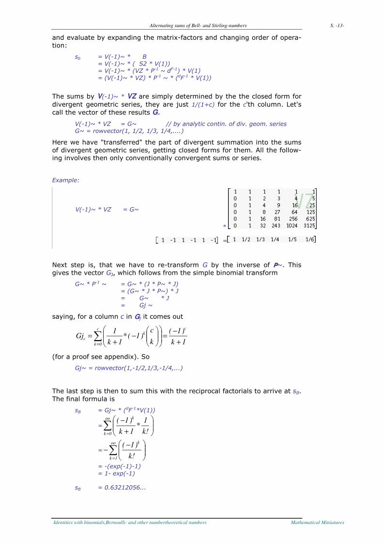
and evaluate by expanding the matrix-factors and changing order of opera-

tion:

sb = V(-1)~ * B

= V(-1)~ * ( S2 * V(1))

= V(-1)~ * (VZ * P-1 ~ dF-1) * V(1)

= (V(-1)~ * VZ) * P-1 ~ * (dF-1 * V(1))

The sums by V(-1)~ * VZ are simply determined by the the closed form for

divergent geometric series, they are just 1/(1+c) for the c'th column. Let's

call the vector of these results G.

V(-1)~ * VZ = G~ // by analytic contin. of div. geom. series

G~ = rowvector(1, 1/2, 1/3, 1/4,....)

Here we have "transferred" the part of divergent summation into the sums

of divergent geometric series, getting closed forms for them. All the follow-

ing involves then only conventionally convergent sums or series.

Example:

V(-1)~ * VZ = G~

*

=

Next step is, that we have to re-transform G by the inverse of PPPP~. This

gives the vector GJ, which follows from the simple binomial transform

G~ * P-1 ~ = G~ * (J * P~ * J)

= (G~ * J * P~) * J

= G~ * J

= Gj ~

saying, for a column c in GGGGj it comes out

∑= +

−=

−

+=

c

0k

ck

c1k

)1(

k

c)1(*

1k

1Gj

(for a proof see appendix). So

Gj~ = rowvector(1,-1/2,1/3,-1/4,...)

The last step is then to sum this with the reciprocal factorials to arrive at sB.

The final formula is

sB = Gj~ * (dF-1*V(1))

=∑=

+

−oo

0k

k

!k

1*

1k

)1(

= ∑=

−−

oo

1k

k

!k

)1(

= -(exp(-1)-1)

= 1- exp(-1)

sB = 0.63212056...



So the full decomposition of the summation-process for the alternating sum

of Bell-numbers is

sB = V(-1)~ * B

= V(-1)~ * ( S2 * V(1))

= V(-1)~ * (VZ * P-1 ~ dF-1) * V(1)

= (V(-1)~ * VZ) * P-1 ~ * (dF-1 * V(1))

= ( G~ * J P~) J * dF-1 * V(1)

= ( Gj~ )* dF-1 * V(1)

= -(exp(-1)-1)

= 1- exp(-1)

sB = 0.63212056...

which agrees perfectly with the result, which I approximated using the Ri-

esz-summation.

It is interesting, that as part of these derivations we have also determined

the alternating sum of the Stirling numbers 2nd kind themselves: they are

just the individual terms of the last formula in the previous. Only we should

normalize for the sign, since the sums begin at different index (r=0,1,2,3,...

for column c=0,1,2,3,...) while the index of the negative signs of their coef-

ficients is the same for all columns.

From

V(-1)~ * B = V(-1)~ * S2 * V(1)

= Gj~ * dF-1 * V(1)

we need only remove the last vectorial summation V(1) to get the vector

ASASASASS2 of that individual sums, and append one dJ-multiplication for sign-

correction:

Y1~ =V(-1)~ * S2 // the uncorrected matrix-product

= Gj ~ * dF-1

ASS2~ = Y1~ * dJ // use J for correction of sign-offsets

= rowvector(1,1/2!,1/3!,1/4!,...)

or said differently, for a column c of S2S2S2S2 we have the following finite value for

its divergent alternating sum, if the sum begins always at +1:

( )∑=

+

+=−

oo

0r

c,r

cr

)!1c(

12S*)1( // divergent summation



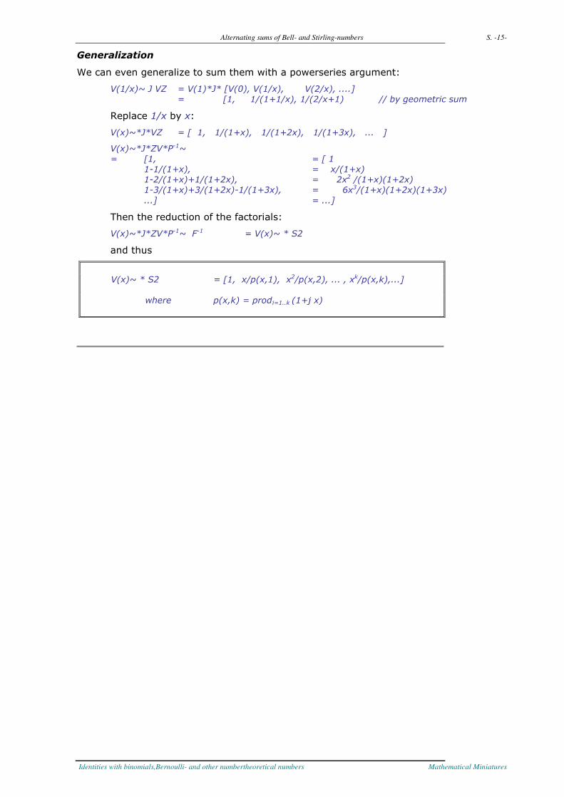
Generalization

We can even generalize to sum them with a powerseries argument:

V(1/x)~ J VZ = V(1)*J* [V(0), V(1/x), V(2/x), ....]

= [1, 1/(1+1/x), 1/(2/x+1) // by geometric sum

Replace 1/x by x:

V(x)~*J*VZ = [ 1, 1/(1+x), 1/(1+2x), 1/(1+3x), ... ]

V(x)~*J*ZV*P-1~

= [1, = [ 1

1-1/(1+x), = x/(1+x)

1-2/(1+x)+1/(1+2x), = 2x2 /(1+x)(1+2x)

1-3/(1+x)+3/(1+2x)-1/(1+3x), = 6x3/(1+x)(1+2x)(1+3x)

...] = ...]

Then the reduction of the factorials:

V(x)~*J*ZV*P-1~ F-1 = V(x)~ * S2

and thus

V(x)~ * S2 = [1, x/p(x,1), x2/p(x,2), ... , xk/p(x,k),...]

where p(x,k) = prodj=1..k (1+j x)



2.2. Alternating sum of B(2)-numbers

Using the previous result, we may simply proceed:

B(2) = S22 * V(1)

sB2 = V(-1)~ * B(2) // its alternating sum

= V(-1)~ * S2 * B

= V(-1)~ * S2 * S2 * V(1)

= V(-1)~ * (VZ*P-1~*dF-1) * S2 * V(1)

= (V(-1)~ * VZ*P-1~) * (dF-1 * S2) * V(1)

= (Z(1)~*J) * (dF-1 * S2) * V(1)

= ( Gj ~ * dF-1* S2) * V(1) // Gj =[1,-1/2,1/3,...]

// from the previous paragraph

Here the product G G G G j~* dF-1*S2S2S2S2 implies evaluation of convergent series only,

so we can give very well approximations for the first part:

G2~ = Gj~ * dF-1 * S2

and we get the approximations

G2~ = rowvector( 1, -0.36788, 0.084046, -0.013983, 0.0018326,

-0.00019831, 0.000018284, -0.0000014690,...)

The sum is again convergent, we get by serial summation:

sB2 = G2 ~ * V(1) = 0.703834423154...

and thus

sB2 = V(-1)~ * B(2)

= 0.703834423154...



But there is also a full analytical description possible, using two terms of the

exponential-integral-function EI() only.

If we proceed as in the previous chapter and apply the VZ VZ VZ VZ *PPPP-1~ * dFFFF-1 trans-

formation we get

sB2 = Gj ~ * dF-1 * (VZ * P-1~ * dF -1) * V(1)

= (Gj ~ * dF-1* VZ) * (P-1~ * dF -1 * V(1) )

= Y2 ~ * dF -1*1/e

For Y2 we get by Gj = [1, -1/2, 1/3, -1/4,...]

Y2 = [1, 1-e-1, (1-e-2)/2, (1-e-3)/3, ...]

So (Y2 * dF-1 )/e leads then to

SB2 ∑=

−−

−+=

inf

1k

k1

!k

1*

k

e11(e

Since this expression is convergent, we may separate the terms to get

SB2 )!k*k

e

!k*k

11(e

inf

1k

kinf

1k

1 ∑∑=

−

=

−

−

+=

The sum-terms in this agree to the sum-terms in the exponential-integral

function Ei() (see [A&S], pg.229])

Ei(x) = gamma + ln(x) + ∑=

oo

1k

k

!k*k

x // x>0

such that the sum sB2 can be expressed

sB2 =e-1(1+ (Ei(1) - ln(1) - gamma) – (Ei(e-1) - ln(e-1) - gamma))

which reduces to

sB2 =e

)(Ei)1(Eie1−

= 0.703834423154 3

I didn't derive the sums for higher-order Bell-numbers yet.

3 in the Pari/Gp-implementation

gp > e = exp(1)

gp > EI(x) = (- eint1(-x)) //define EI-function

gp > ( EI(1) - EI(1/e)) /e

%558 = 0.703834423154



2.3. Alternating sum of B(m) of same index

To determine the alternating sums of B(m) over all m of a fixes index r is not

difficult. The B(m)r grow according to the r'th polynomial and thus Euler- or

even Cesaro-summation is sufficient. But it is even simpler: since the re-

lated polynomials are just finite linear combinations of an *mn , with an

some coefficients, we may replace this using the alternating zeta-function,

the Dirichlet eta-function η(), at non-positive integer arguments.

However, different from that definition, we need a variant, where the index

of the η() function begins at zero, denote it as η°() with the effect, that its

sign is changed except for k=0:

def: η°(-k) = 0k-η(-k)

Then

( )

( )

( )

( )∑

∑ ∑

∑ ∑

∑

=

= =

= =

=

−=

−=

−=

−=

n

0k

o

k

n

0k

oo

0m

km

k

oo

0m

n

0k

k

k

m

oo

0m

m

n

m

n

)k(a

m)1(a

m*a)1(

b)1(s

η

Examples. Recall the m-polynomials as given by E.T.Bell, expanded for m:

ξ(m)1 = 1 = 1m0

ξ(m)2 = m + 1 = 1m1 + 1m0

ξ(m)3 = 1/2(m + 1)(3m+2) = (3m2 +5m1 + 2m0)/2

ξ(m)4 = 1/2(m + 1)(2m+1)(3m+2) = (6m3 + 13m2 + 9m1 + 2m0)/2

Then for a fixed row n we get the alternating sum by the formal replace-

ment of mk by η°(-k)

s1 = 1*η°( 0) = 1/2

s2 = 1*η°(-1)+1*η°( 0) = -1/4+1/2 = 1/4

s3 = 3*η°(-2)+5*η°(-1)+2*η°( 0) = (0-5/4+1)/2 = -1/8

...

giving the sequence

s = (1/2, 1/2, 1/4, -1/8, -1/4, 19/16, 39/32, -2623/64, 365/8, 258257/64,... )

and separated for numerators and denominators we get

numerators(sn) = (1, 1, 1, -1, -1, 19, 39, -2623, 365, 258257, ...)

denominators(sn)=(2, 2, 4, 8, 4, 16, 32, 64, 8, 64, ...)



Although these sums don't look as of much interest, I'll show the same

problem in the chosen matrix-notation.

Since B B B B (k) = S2S2S2S2 k * V(1) the alternating sum over k=0..inf of all these vec-

tors is

AB = S20 * V(1) – S21 * V(1) + S22*V(1) - ... + ...

= (S20 – S21 + S22 – S23 + ... -...) * V(1)

= (I + S2)-1 * V(1)

where in the last row I applied the closed form for the alternating geometric

series to the matrix-argument.

The shortness of this formula is impressive. We get the matrix S2AS2AS2AS2A by

S2A = (I + S2)-1

Example:

S2A = (I + S2)-1

and for the required alternating sums

AB = S2A * V(1)

we get the vector

AB = [1/2, 1/2, 1/4, -1/8, -1/4, 19/16, 39/32, -2623/64,...]

where the entries give the same results as before.

Example:

AB = S2A * V(1)



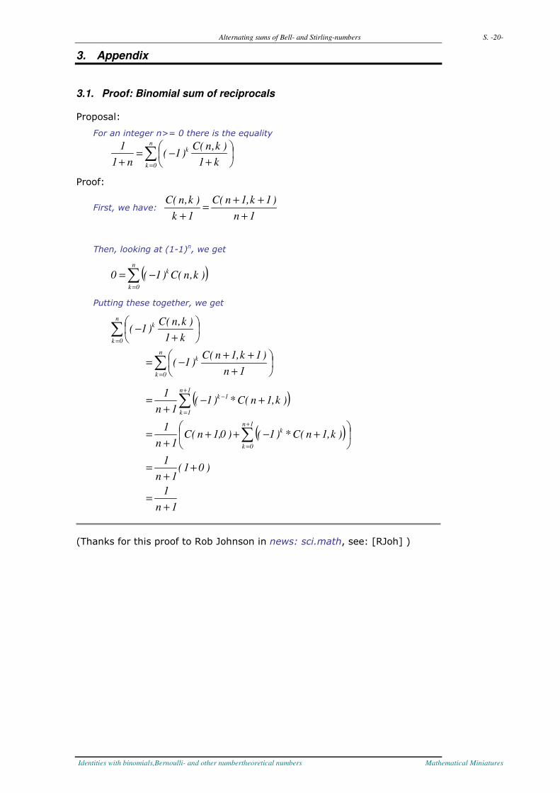
3. Appendix

3.1. Proof: Binomial sum of reciprocals

Proposal:

For an integer n>= 0 there is the equality

∑=

+−=

+

n

0k

k

k1

)k,n(C)1(

n1

1

Proof:

First, we have: 1n

)1k,1n(C

1k

)k,n(C

+

++=

+

Then, looking at (1-1)n, we get

( )∑=

−=n

0k

k)k,n(C)1(0

Putting these together, we get

∑

∑

=

=

+

++−=

+−

n

0k

k

n

0k

k

1n

)1k,1n(C)1(

k1

)k,n(C)1(

( )

( )

1n

1

)01(1n

1

)k,1n(C*)1()0,1n(C1n

1

)k,1n(C*)1(1n

1

1n

0k

k

1n

1k

1k

+=

++

=

+−++

+=

+−+

=

∑

∑+

=

+

=

−

(Thanks for this proof to Rob Johnson in news: sci.math, see: [RJoh] )



4. References

[A&S] Milton Abramowitz, I. A. Stegun (Eds.).; "Handbook of Mathematical Functions..." "Stirling Numbers of the Second Kind." §24.1.4 Definin. B and C New York: Dover, 1972. p. 824 (9th printing) Online-copy: http://www.math.sfu.ca/~cbm/aands/page_824.htm

(as before) page 229 Online-copy: http://www.math.sfu.ca/~cbm/aands/page_229.htm

[Bell38] E.T.Bell; "The Iterated Exponential Integers" in: The Annals of Mathematics, 2nd Sr.,Vol.39,No.3 (Jul. 1938) online access (restricted): http://www.jstor.org/pss/1968633

[Knopp] Konrad Knopp; "Theorie und Anwendung der unendlichen Reihen" Springer, 1964; online access (free): Digicenter University Goettingen

[Pbal] Pat Ballew; "The Bell Numbers" http://www.pballew.net/Bellno.html

[OEIS] Neill J.A. Sloane; The online encyclopedia of Integer Sequences http://www.research.att.com/~njas/sequences/

c=1 Bell or exponential numbers: http://www.research.att.com/~njas/sequences/A000110 c=2 Number of 3-level labeled rooted trees with n leaves. http://www.research.att.com/~njas/sequences/A000258 c=3 Number of 4-level labeled rooted trees with n leaves. http://www.research.att.com/~njas/sequences/A000307 c=4 Number of 5-level labeled rooted trees with n leaves. http://www.research.att.com/~njas/sequences/A000357 c=5 Number of 6-level labeled rooted trees with n leaves. http://www.research.att.com/~njas/sequences/A000405

[RJoh] Rob Johnson, "re:looking for a proof for binomial-transform of harmonic series" 22.5..08 news:[email protected]

[Weiss] Eric Weissstein; "Bell-numbers" in: Eric Weissstein's Mathworld; see De Bruin's formula (1958) eq.10 http://mathworld.wolfram.com/BellNumber.html

For another generalization of Bell-numbers of higher orders see:

[JIS] J.-M. Sixdeniers, K. A. Penson, A. I. Solomon; "Extended Bell and Stirling Numbers From Hypergeometric Exponentiation" in: Journal of Integer Sequences, Vol. 4 (2001),Article 01.1.4 online at: http://www.emis.de/journals/JIS/VOL4/SIXDENIERS/bell.pdf

[Pari] the Pari/GP-group http://pari.math.u-bordeaux.fr/

[Project-Index] http://go.helms-net.de/math/binomial/index

[Intro] http://go.helms-net.de/math/binomial/intro.pdf

[Stir] Description and some heuristics on Stirling-matrices http://go.helms-net.de/math/binomial_new/01_3_stirling.pdf

Thanks to Dave L. Renfro who hinted me to the article of E.T.Bell recently Rob Johnson for the proof of the binomial-identity Pari/GP-group for providing the free computer-algebra-program

The bitmaps for the example are produced with the bitmap-facility of my Pari/GP-GUI Pari-TTY http://go.helms-net.de/sw/paritty

email of author: helms(at)uni-kassel.de

Documents

04 5 SummingBellStirling - Index Homepage Gottfried · PDF fileAlternating sums of Bell- and Stirling-numbers S. -2- Identities with binomials,Bernoulli- and other numbertheoretical