Embed Size (px)
Citation preview
03/10/051
Geometric Facility Location Optimization
Class #8, CG in action (applications)
03/10/052
Class 8 - agenda:
• Projects:– Who does what, when (presentation dates).– Cross-projects cooperation
• CG in action: some applications– Visibility, Connectivity.– Simplification, approximation.– Facility Location Optimization
03/10/053
Ex3 – guarding a polygon
• Questions?
• Implementations: – Classes– Benchmarks (guarding tasks / results)
• GUI?
03/10/054
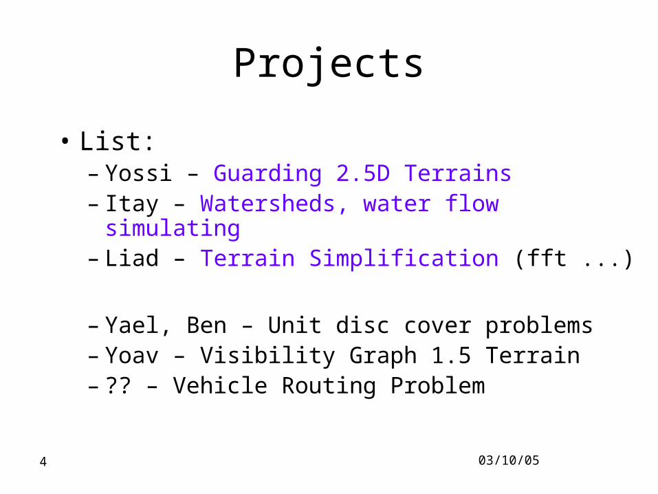
Projects
• List: – Yossi – Guarding 2.5D Terrains– Itay – Watersheds, water flow simulating– Liad – Terrain Simplification (fft ...)
– Yael, Ben – Unit disc cover problems– Yoav – Visibility Graph 1.5 Terrain– ?? – Vehicle Routing Problem
03/10/055
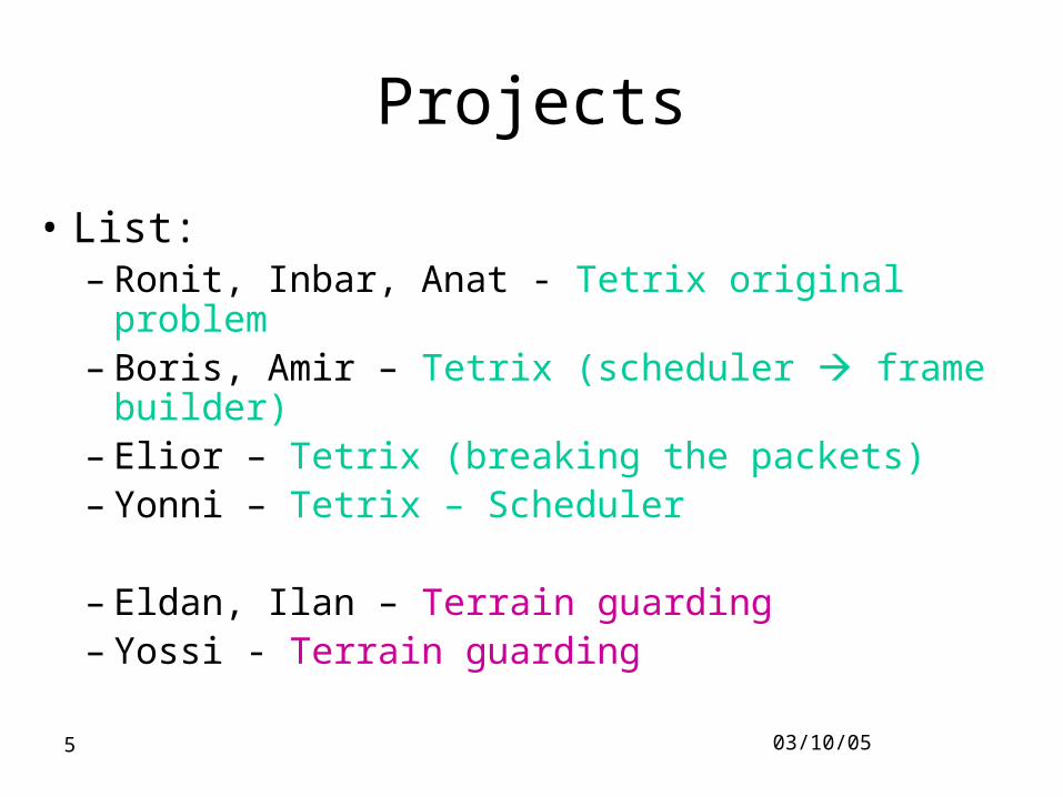
Projects
• List: – Ronit, Inbar, Anat - Tetrix original problem– Boris, Amir – Tetrix (scheduler frame builder)– Elior – Tetrix (breaking the packets)– Yonni – Tetrix – Scheduler
– Eldan, Ilan – Terrain guarding– Yossi - Terrain guarding

03/10/056
Projects
• Others?
• Start ASAP
• Work together: maps, experiments.
• Presentations: class 10-11: when?
03/10/057
Geometric Facility Location Optimization
CG applications example:LSRT project:
Locating large scale wireless network
03/10/058
Geometric Facility Location Optimization:• Computational Geometry• Facility Location• Optimization• Application
Definition & Motivation

03/10/059
Real life examples – problems:• traffic-lights• Air-ports• Shipping: cargo, delivery, etc.• Wireless networks
Definition & Motivation
03/10/0510
Wireless networks:• LSRT: Large Scale Rural Telephone • telephone & internet service (VoIP).• Input
– Clients: schools, pay-phones, etc.– Base station possible location– Parameters, objective function
Definition & Motivation
03/10/0511
Definition & Motivation
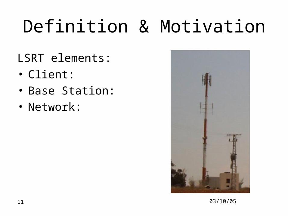
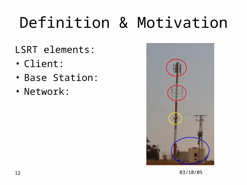
LSRT elements:
• Client:• Base Station:• Network:
03/10/0512
Definition & Motivation
LSRT elements:
• Client:• Base Station:• Network:
03/10/0513
Definition & Motivation
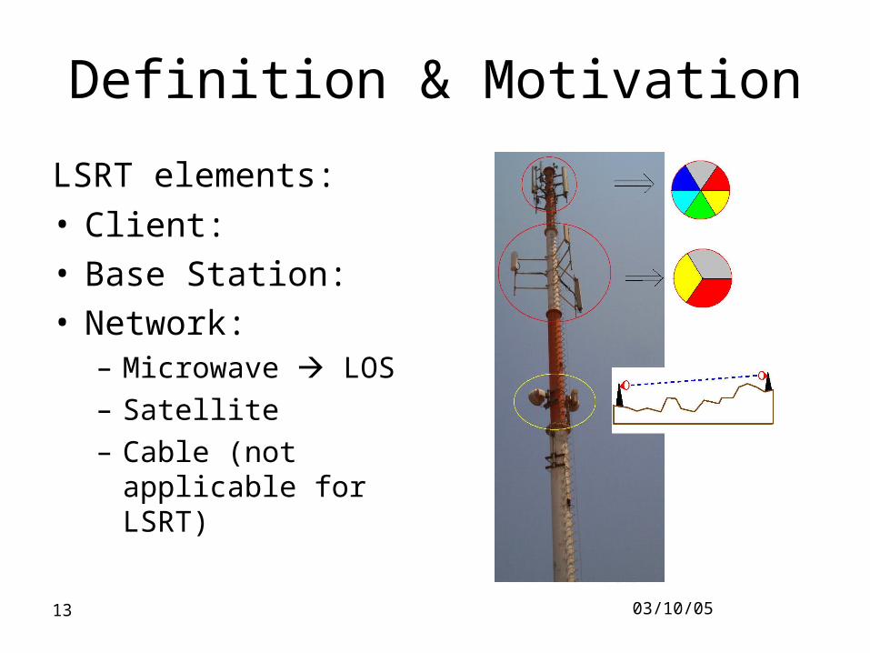
LSRT elements:
• Client:• Base Station:• Network:
– Microwave LOS– Satellite– Cable (not applicable
for LSRT)
03/10/0514
Definition & Motivation
Goal: design an ‘optimal’ LSRT network
Problems of interest:• Locating Base Stations• Frequency Assignment• Connectivity
03/10/0515
Definition & Motivation
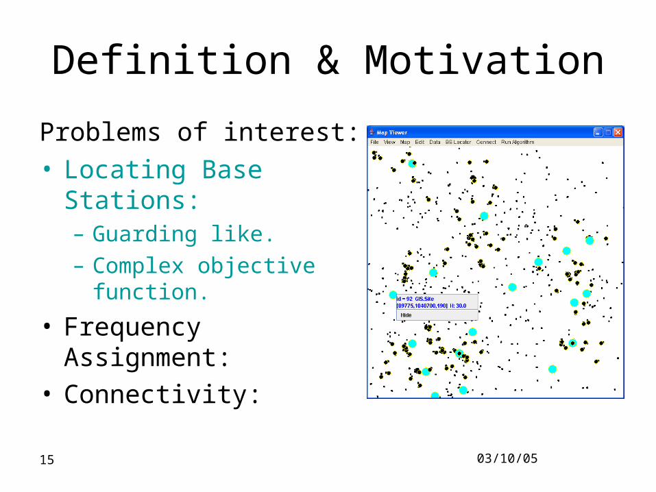
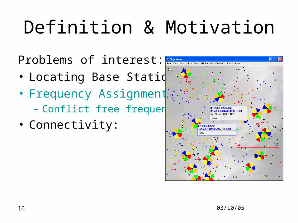
Problems of interest:
• Locating Base Stations:– Guarding like.– Complex objective function.
• Frequency Assignment:• Connectivity:
03/10/0516
Definition & Motivation
Problems of interest:
• Locating Base Stations:• Frequency Assignment:
– Conflict free frequency
• Connectivity:
03/10/0517
Definition & Motivation
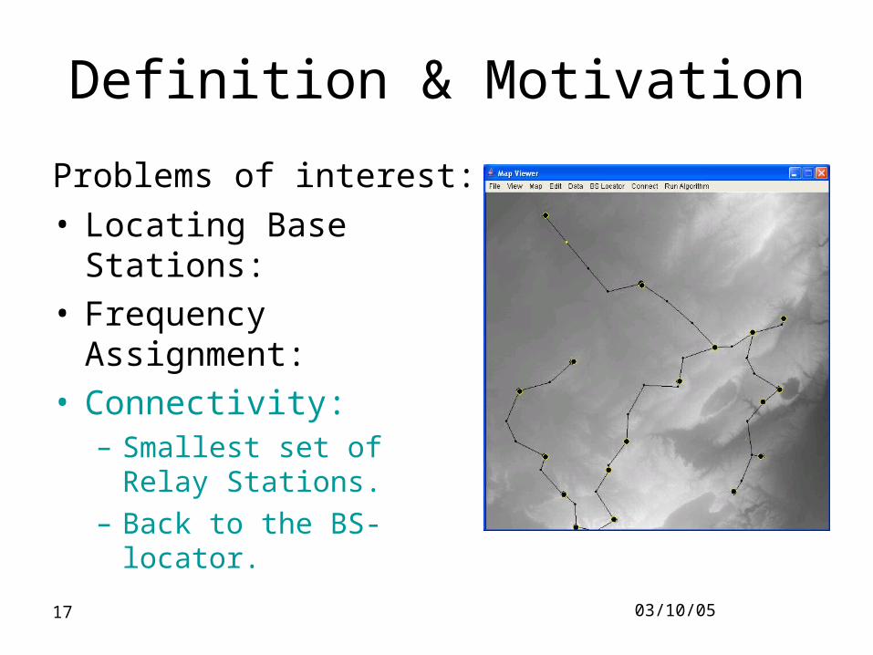
Problems of interest:
• Locating Base Stations:• Frequency Assignment:• Connectivity:
– Smallest set of Relay Stations.
– Back to the BS-locator.
03/10/0518
Main Obstacles:
• Huge inputs simplify & approximation
• Formalizing objective function
• NP hardness efficient Heuristics
03/10/0519
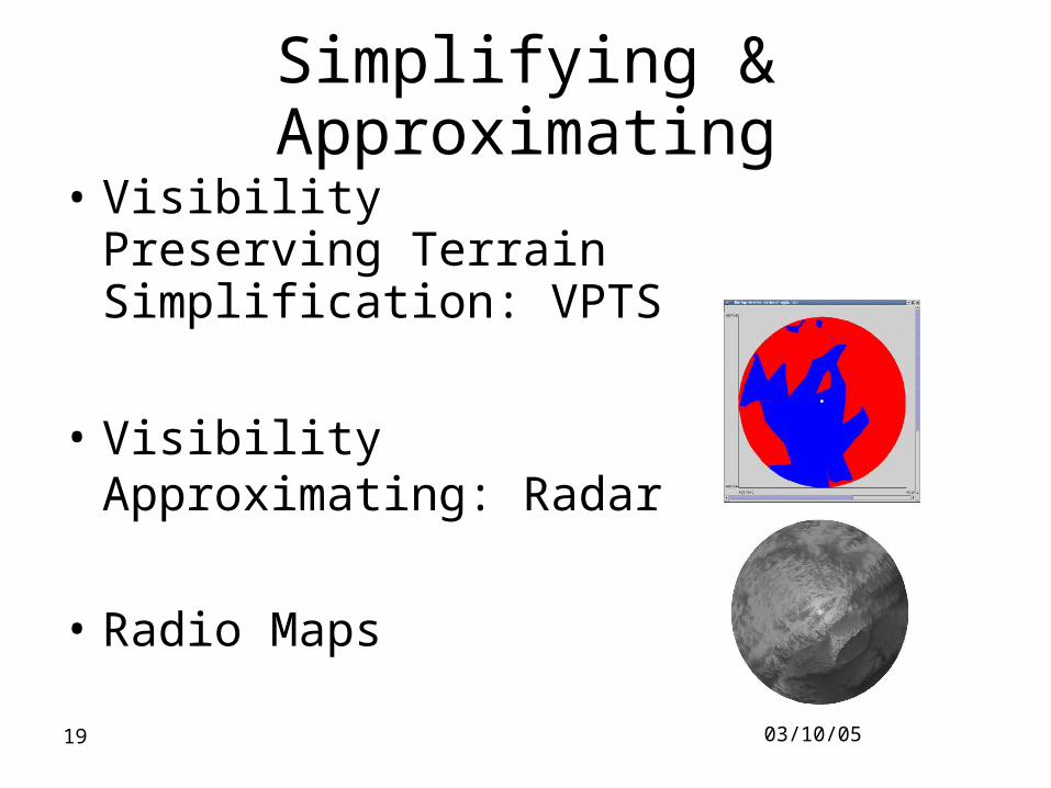
Simplifying & Approximating
• Visibility Preserving Terrain Simplification: VPTS
• Visibility Approximating: Radar
• Radio Maps
03/10/0520
VPTS [BKMN]• Develop a visibility preserving terrain
simplification method - VPTS– Should preserve most of the visibility – Should be efficient
• Define a visibility-based measure of quality of simplification.
• Experiment with VPTS, as well as with other TS methods, using the new quality measure.
03/10/0521
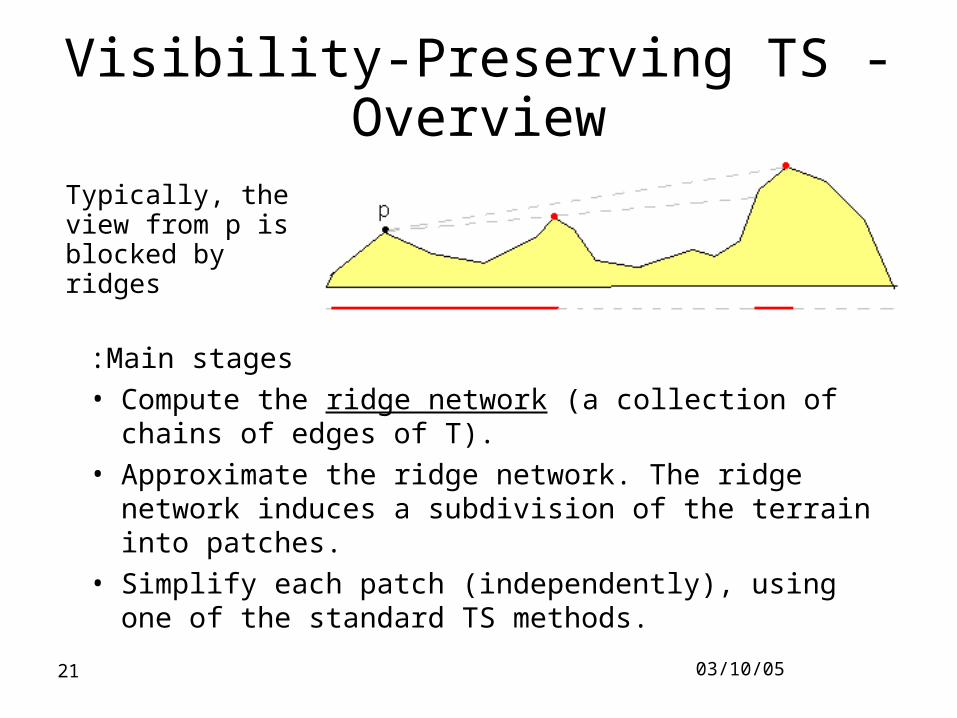
Visibility-Preserving TS - Overview
Main stages:• Compute the ridge network (a collection of chains of
edges of T).• Approximate the ridge network. The ridge network
induces a subdivision of the terrain into patches.• Simplify each patch (independently), using one of the
standard TS methods.
Typically, the view from p is blocked by ridges
03/10/0522
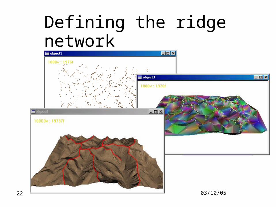
Defining the ridge network
03/10/0523
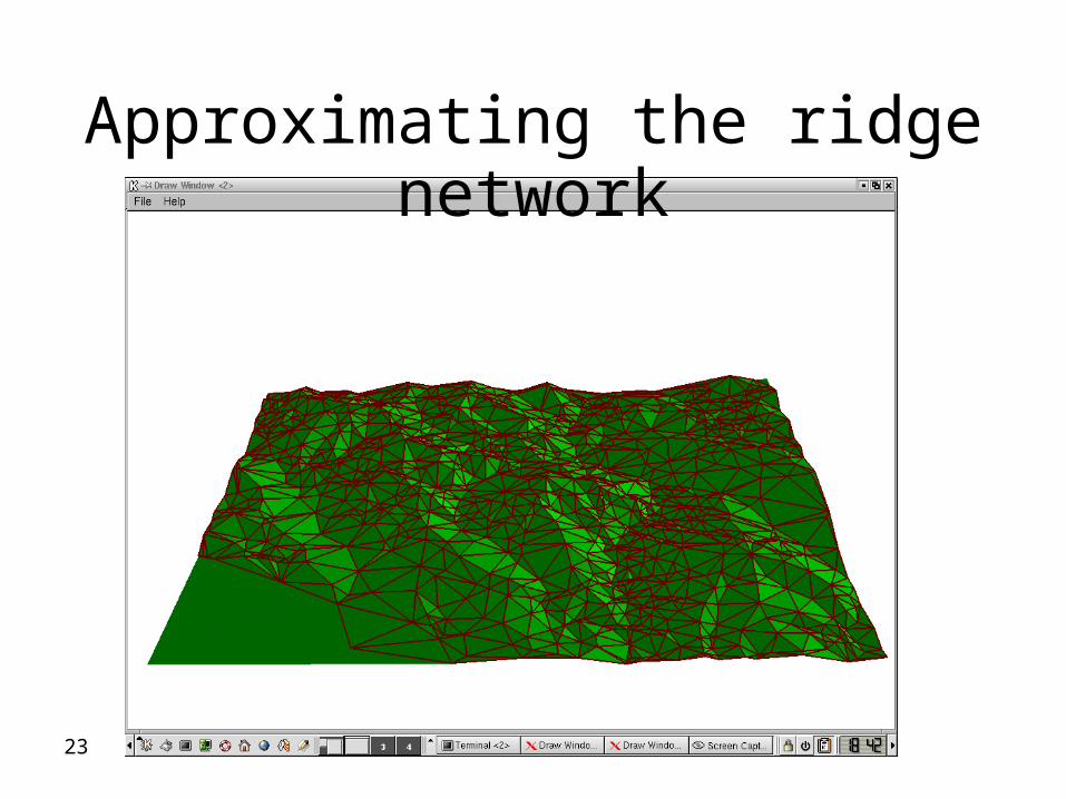
Approximating the ridge network
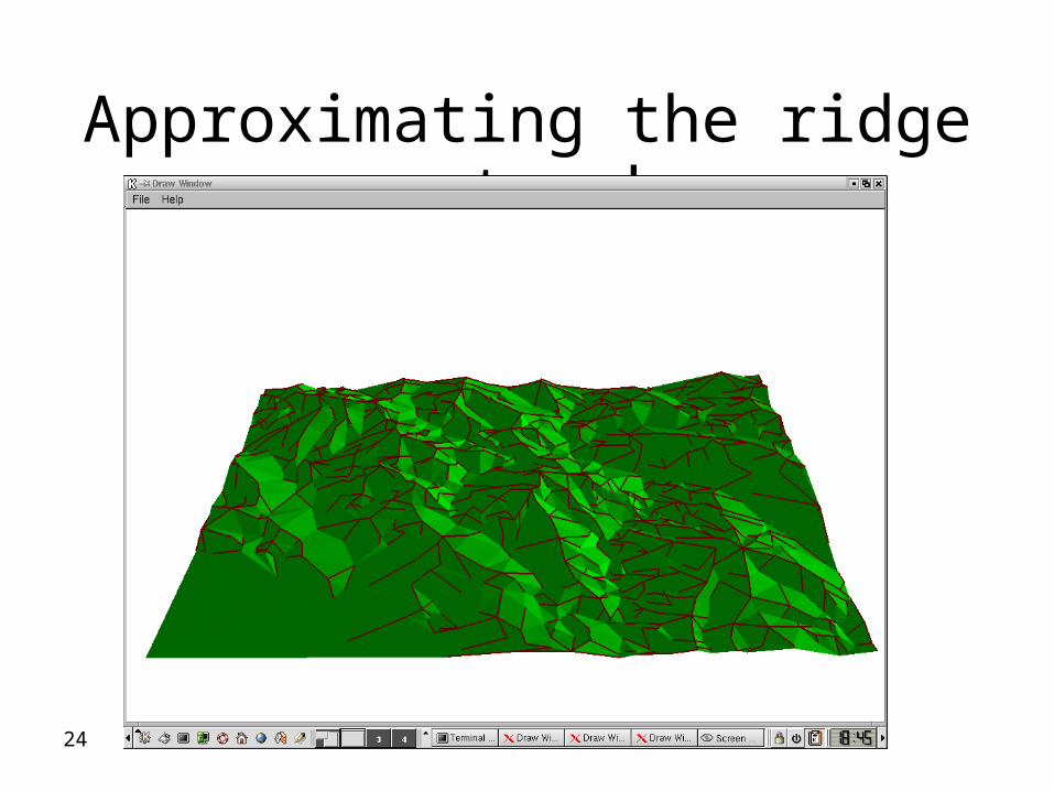
03/10/0524
Approximating the ridge network
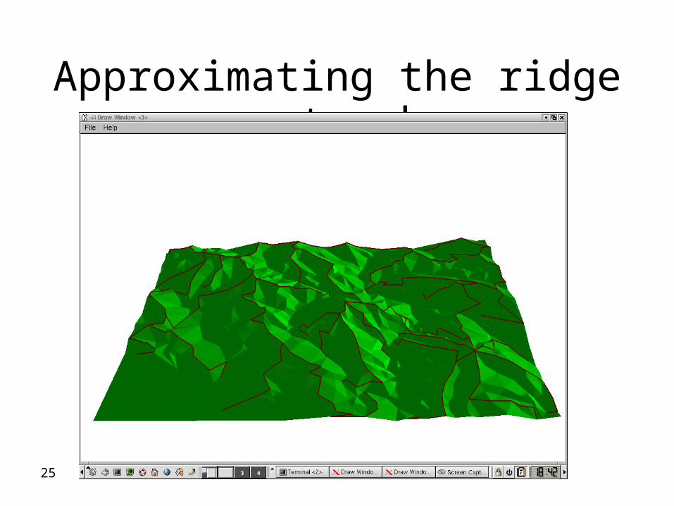
03/10/0525
Approximating the ridge network
03/10/0526
The (simplified) Ridge Network induces a subdivision of the terrain into regions:
• For each region (map[i]) in the subdivision • If map[i] is “big” then recursively apply
VPTS to map[i].• Else (map[i] is “small”) simplify map[i]
using a “standard” simplification method (such as Garland’s “Terra”).
The main TS algorithm
03/10/0527
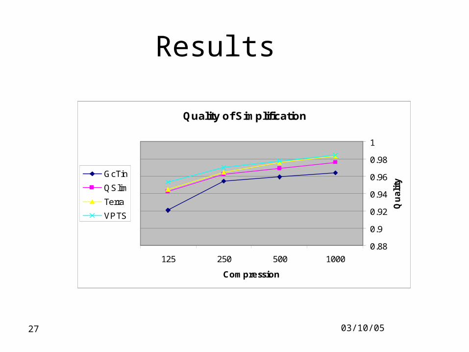
Quality of Simplification
0.88
0.9
0.92
0.94
0.96
0.98
1
1000500250125
Compression
Qu
ali
ty
GcTin
QSlim
Terra
VPTS
Results

03/10/0528
Conclusion
• TS Application.
• Practical Knowledge: Terrain / Grid.
• Accelerating runtime:
7% compress 99.5%
1% compress 98%
03/10/0529
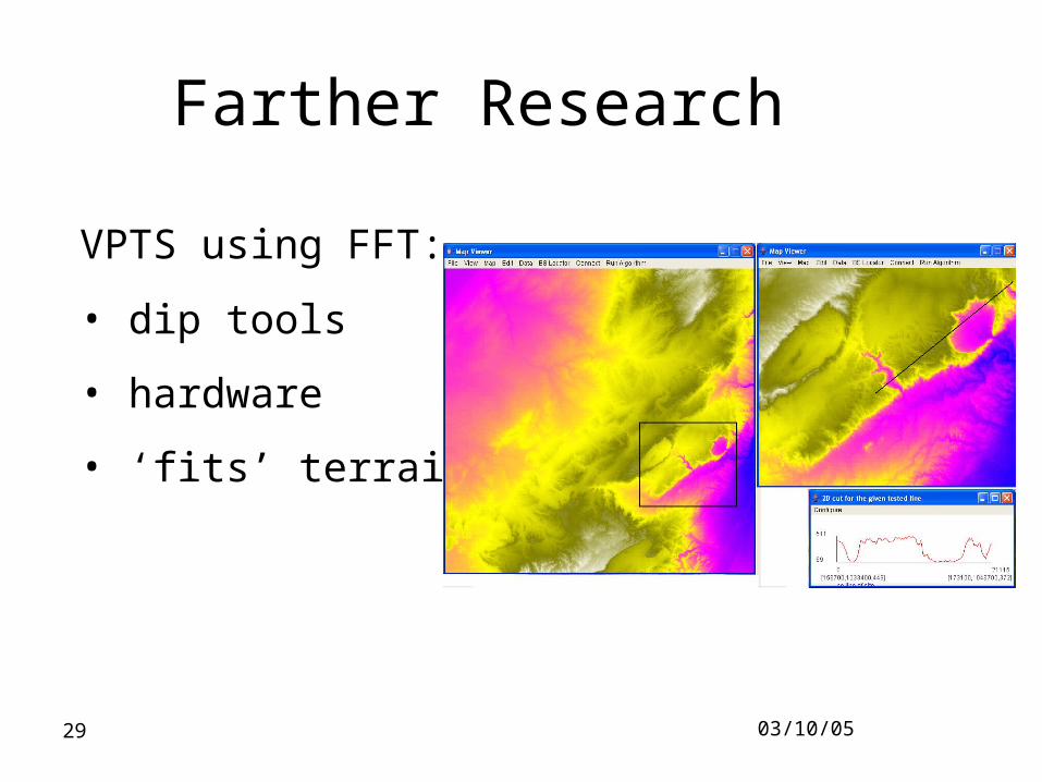
Farther Research
VPTS using FFT:
• dip tools
• hardware
• ‘fits’ terrains

03/10/0530
Approximating Visibility [BCK]
Given a terrain T and a view point p compute the set of points on the surface of T that are visible from p.
Alternatively: Paint T with two colors (red & blue) s.t. any blue (red) point is visible (invisible) from p.
03/10/0531
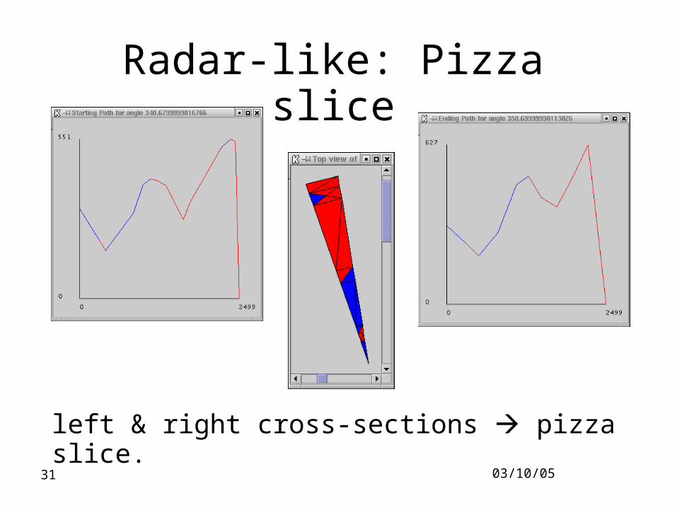
Radar-like: Pizza slice
left & right cross-sections pizza slice.
03/10/0532
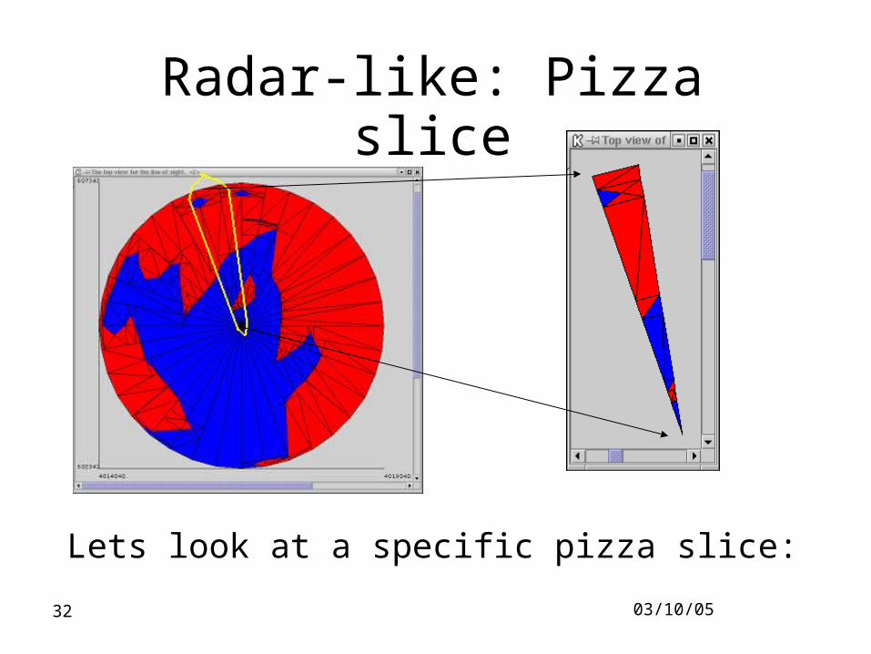
Radar-like: Pizza slice
Lets look at a specific pizza slice:
03/10/0533
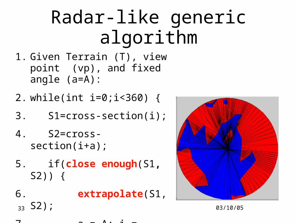
Radar-like generic algorithm
1. Given Terrain (T), view point (vp), and fixed angle (a=A):
2. while(int i=0;i<360) {
3. S1=cross-section(i);
4. S2=cross-section(i+a);
5. if(close enough(S1, S2)) {
6. extrapolate(S1, S2);
7. a = A; i = min(360, i + a);}
8. else a = a/2; }
03/10/0534
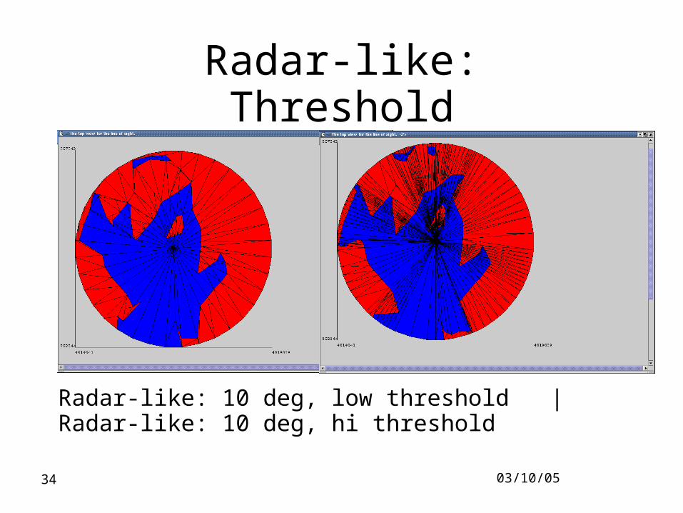
Radar-like: Threshold
Radar-like: 10 deg, low threshold | Radar-like: 10 deg, hi threshold
03/10/0535
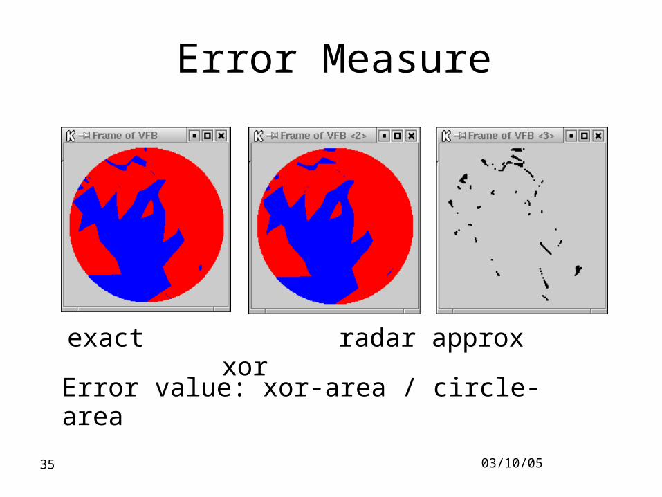
Error Measure
exact radar approx xor
Error value: xor-area / circle-area
03/10/0536
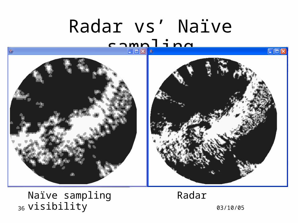
Radar vs’ Naïve sampling
Naïve sampling Radar visibility
03/10/0537
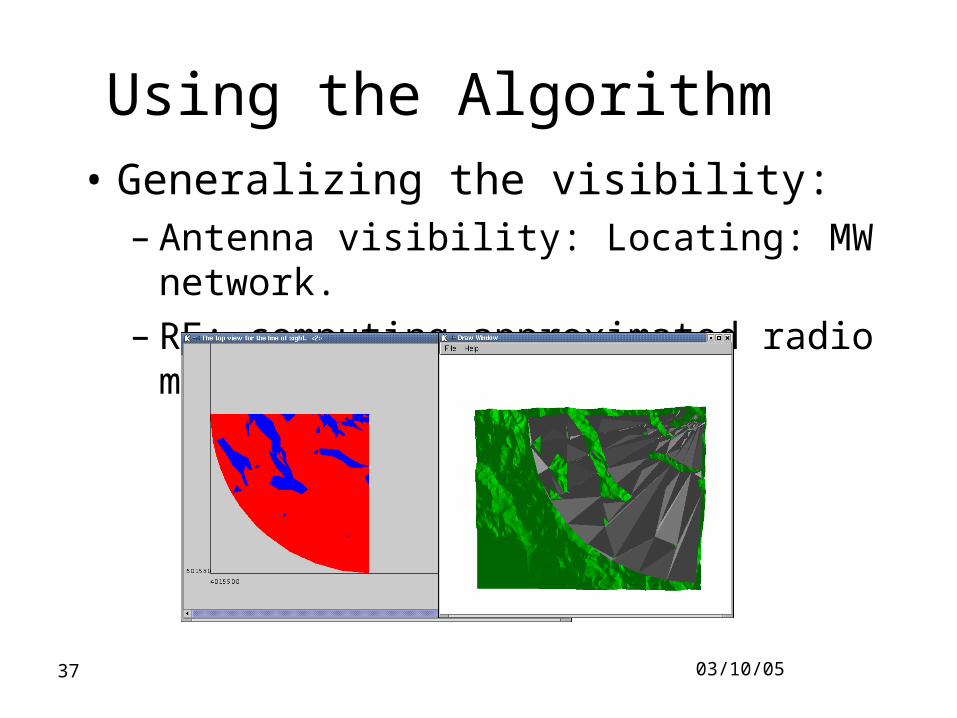
Using the Algorithm• Generalizing the visibility:
– Antenna visibility: Locating: MW network.– RF: computing approximated radio maps.
03/10/0538
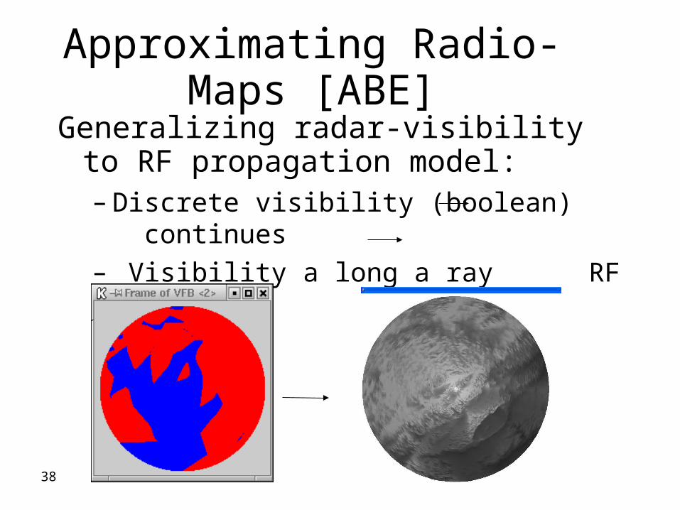
Approximating Radio-Maps [ABE]
Generalizing radar-visibility to RF propagation model:– Discrete visibility (boolean) continues– Visibility a long a ray RF sampling

03/10/0539
Approximating Radio-Maps General Frame work:
Sampling Set (SP) Extrapolation DS
03/10/0540
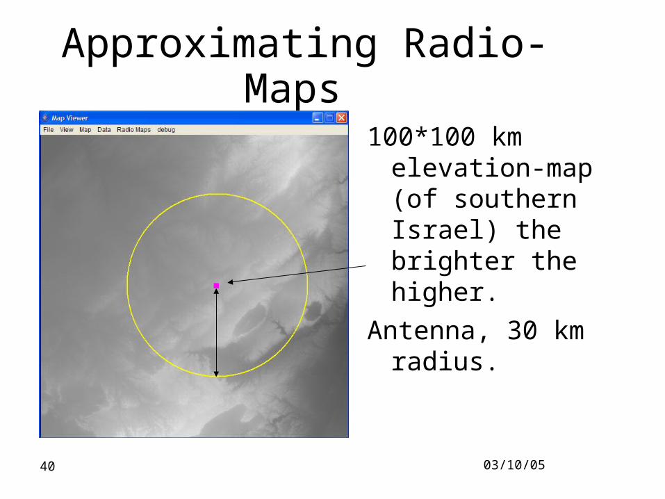
Approximating Radio-Maps
100*100 km elevation-map (of southern Israel) the brighter the higher.
Antenna, 30 km radius.
03/10/0541
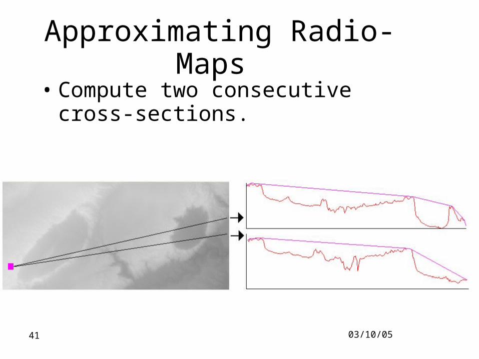
Approximating Radio-Maps • Compute two consecutive cross-
sections.
03/10/0542
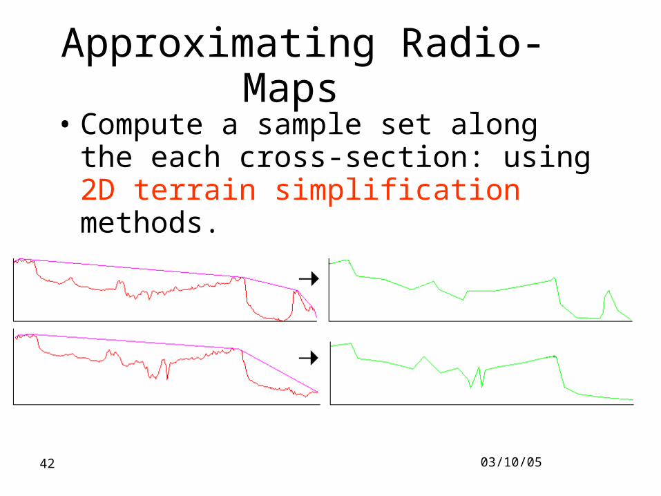
Approximating Radio-Maps • Compute a sample set along the each
cross-section: using 2D terrain simplification methods.
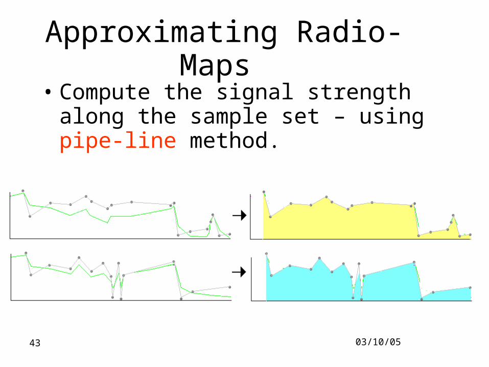
03/10/0543
Approximating Radio-Maps • Compute the signal strength along the
sample set – using pipe-line method.
03/10/0544
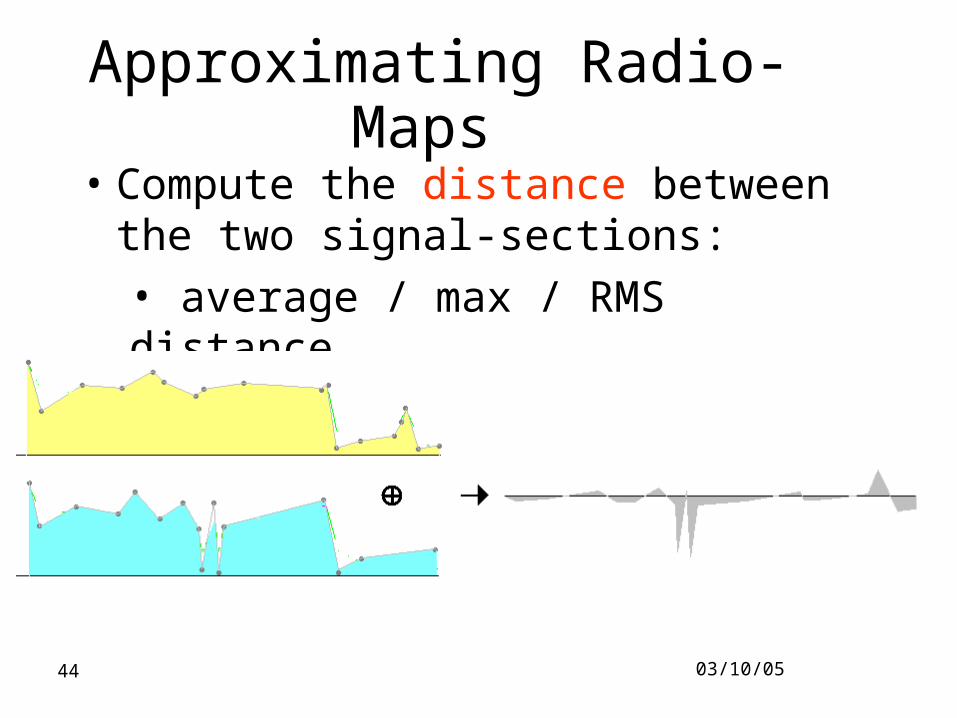
Approximating Radio-Maps
• Compute the distance between the two signal-sections:
• average / max / RMS distance
03/10/0545
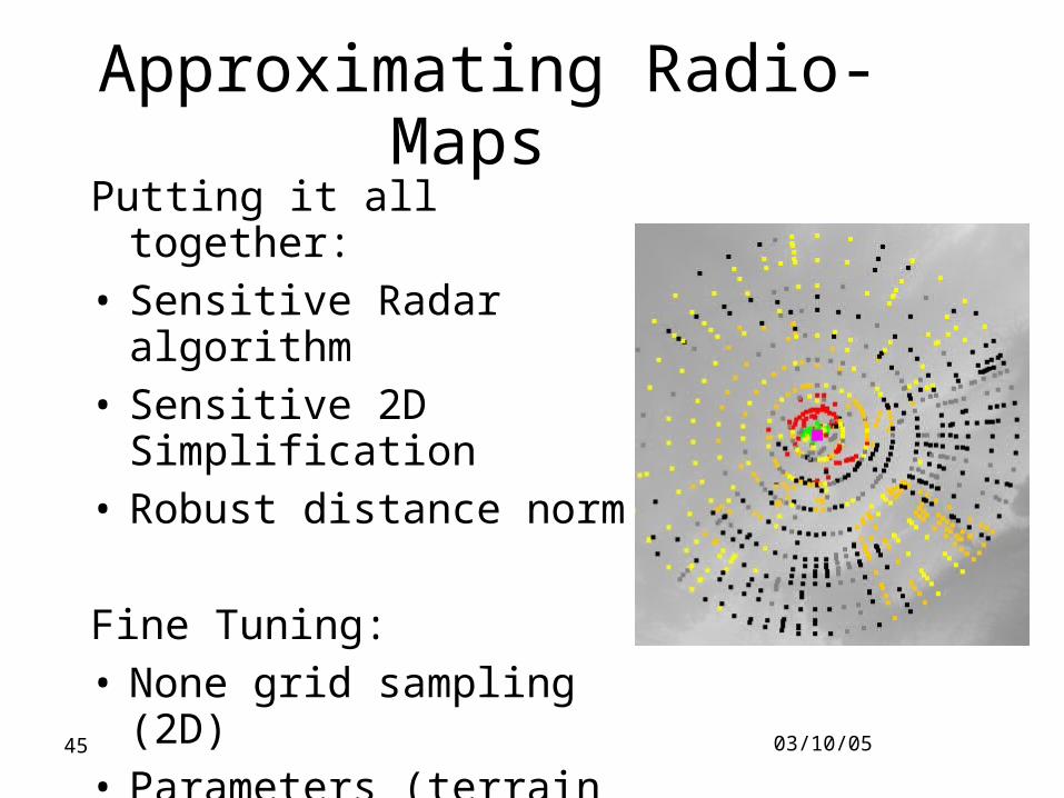
Approximating Radio-Maps Putting it all together:• Sensitive Radar algorithm• Sensitive 2D Simplification• Robust distance norm
Fine Tuning:• None grid sampling (2D)• Parameters (terrain
independent)
03/10/0546
Radio-Maps: resultsMethods:
• Random, Grid, TS
• F-Radar: fixed angle
• S-Radar: sensitive angle
• A-Radar: advance sampling
03/10/0547
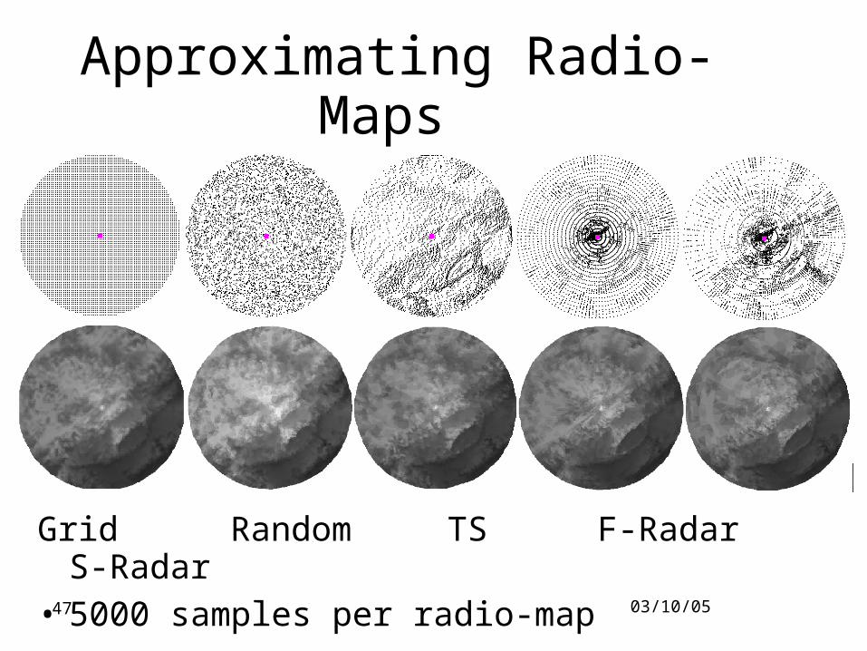
Approximating Radio-Maps
Grid Random TS F-Radar S-Radar
• 5000 samples per radio-map
03/10/0548
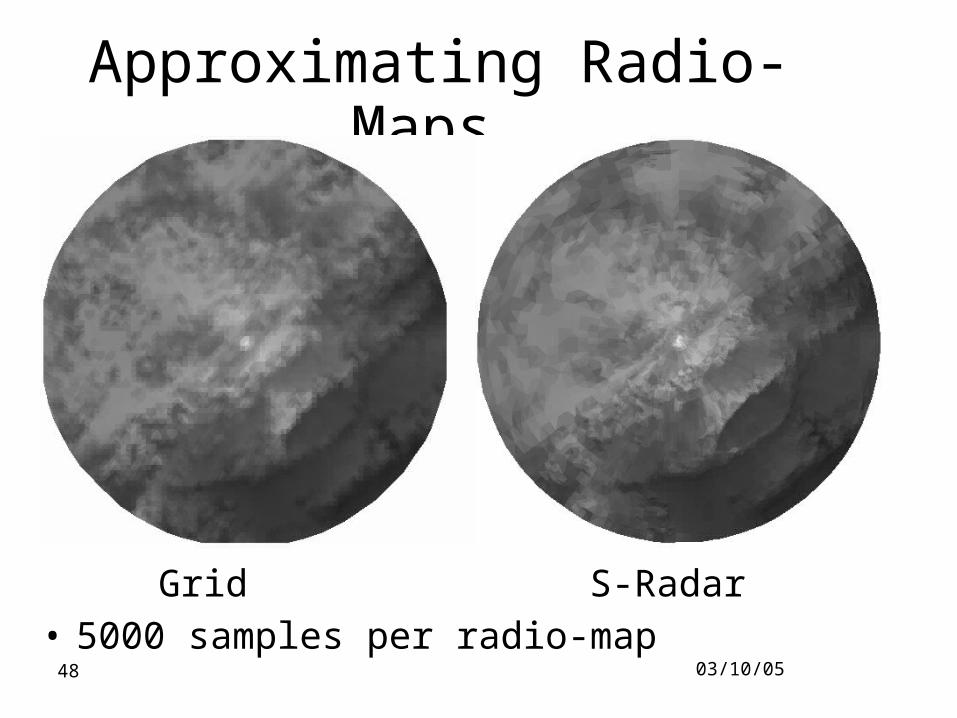
Approximating Radio-Maps
Grid S-Radar• 5000 samples per radio-map
03/10/0549
Radio-Maps: resultsRun time for the same size sampling.
• The radar is 3-15 times faster than the regular sampling Radio Map methods.
• More accurate.

03/10/0550
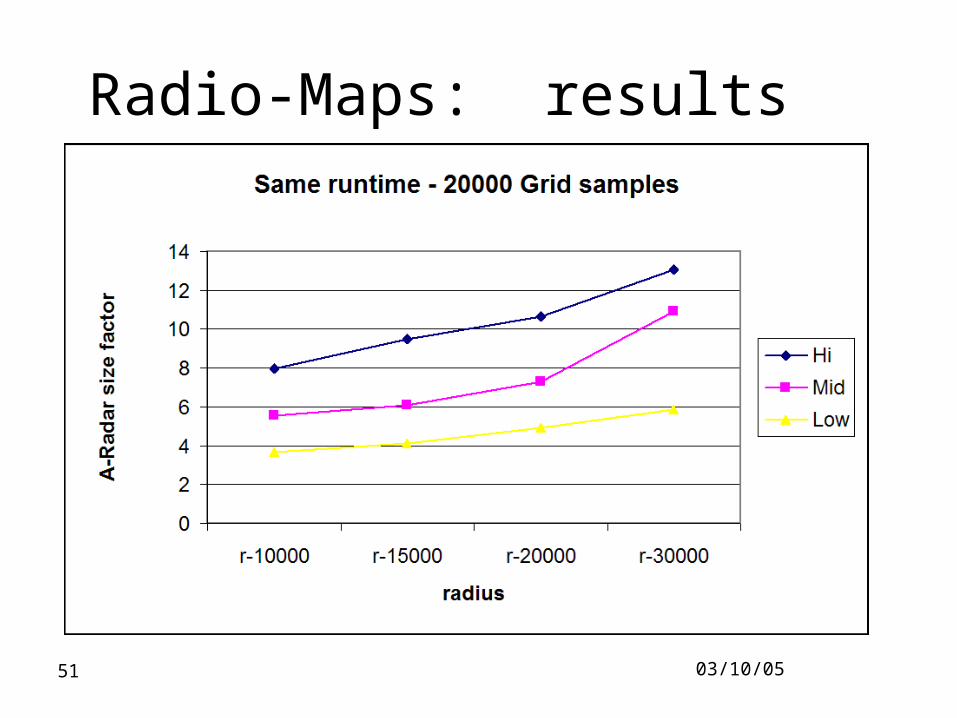
Radio-Maps: results
03/10/0551
Radio-Maps: results
03/10/0552
Future Research• Advance interpolation methods
• Interferences
• Urban, sort-range
http://www.cs.bgu.ac.il/~benmoshe/RadioMaps/
03/10/0553
Expert System
Main Goal: theory practice
• Maps & Geometry & RF model
• Locating Base Stations.
• Frequency Allocation.
• Connecting Base Stations.
03/10/0554
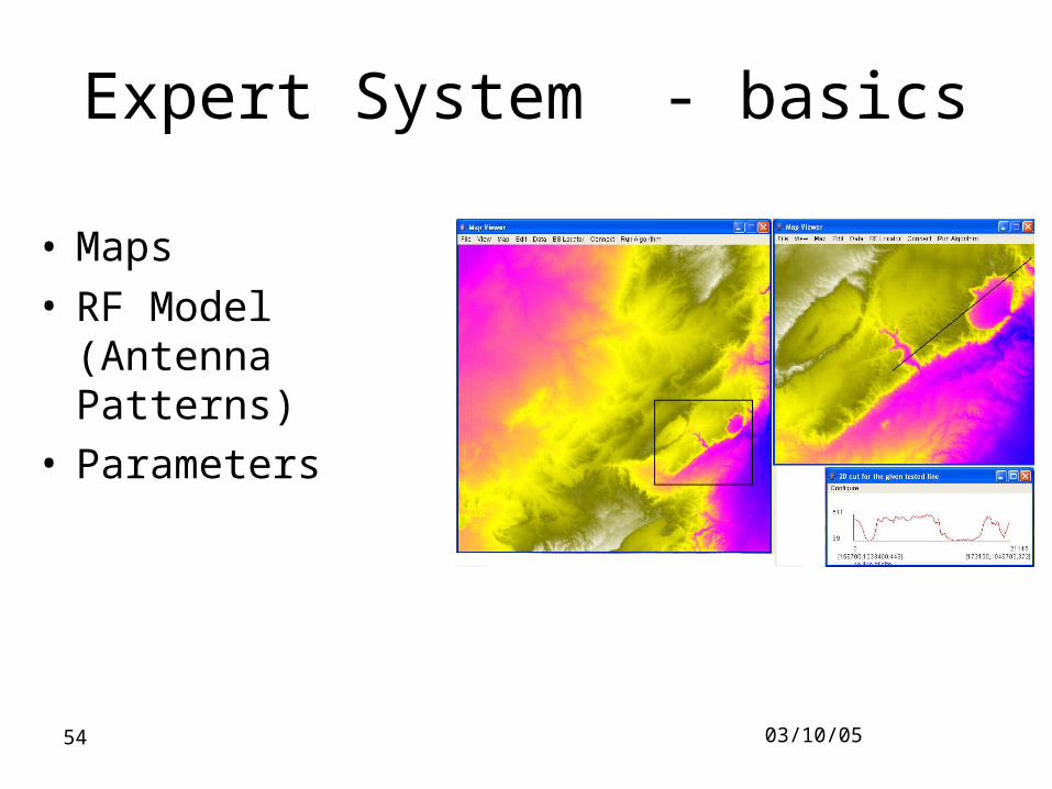
Expert System - basics
• Maps
• RF Model (Antenna Patterns)
• Parameters
03/10/0555
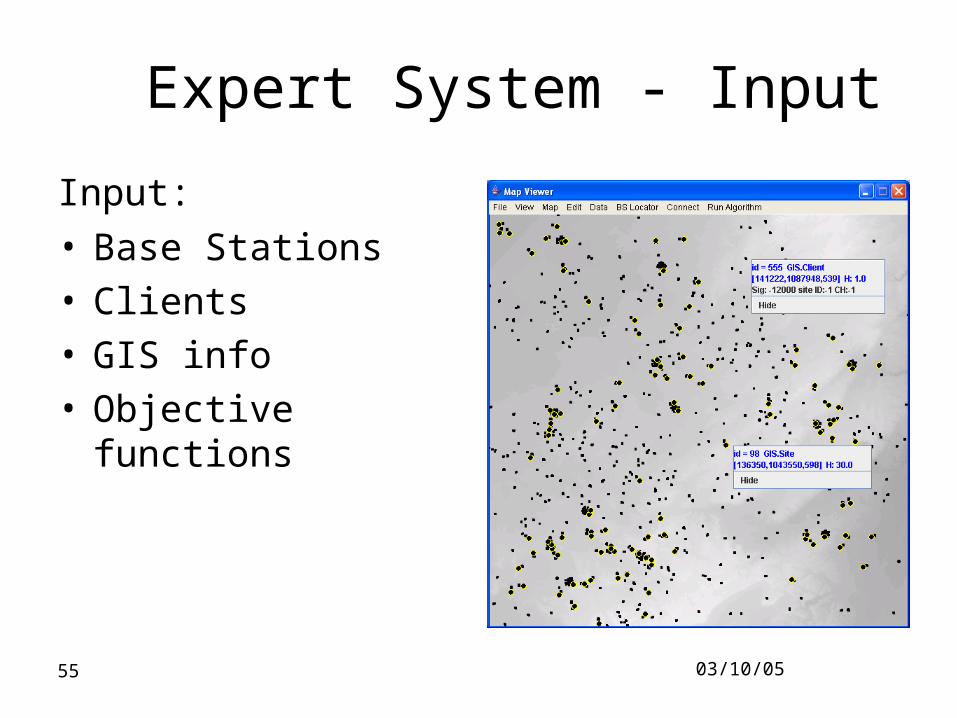
Expert System - Input
Input:
• Base Stations• Clients• GIS info • Objective functions
03/10/0556
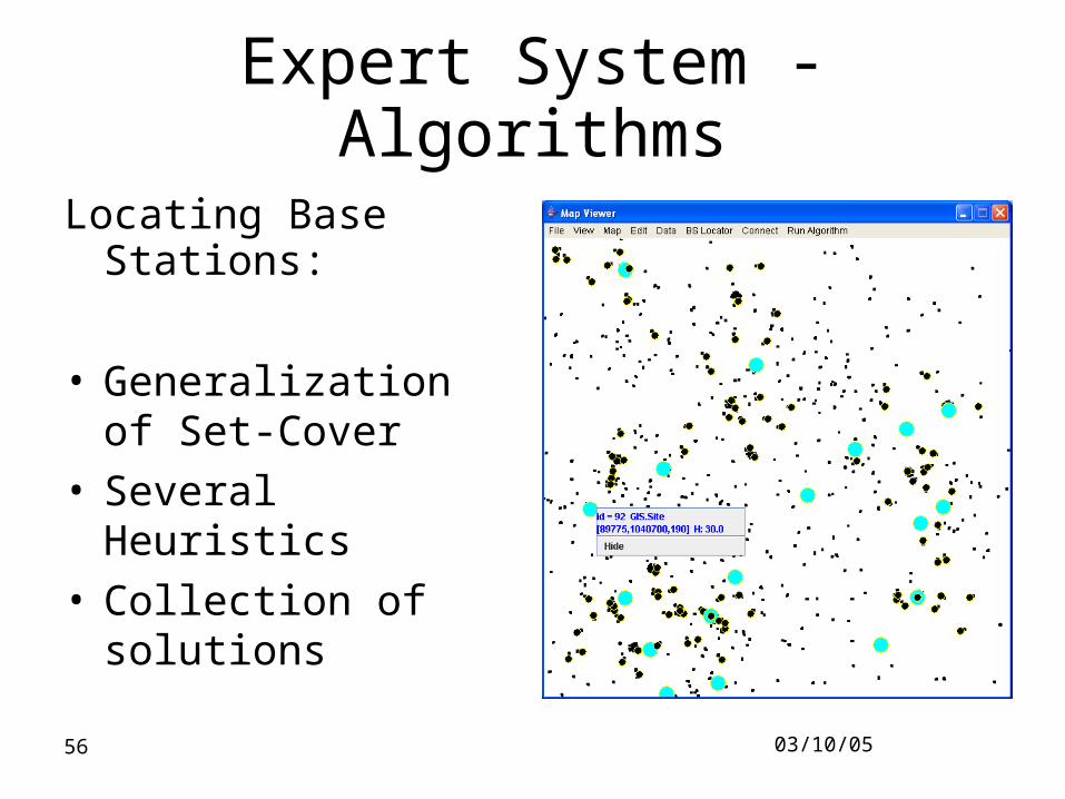
Expert System - Algorithms
Locating Base Stations:
• Generalization of Set-Cover
• Several Heuristics • Collection of solutions
03/10/0557
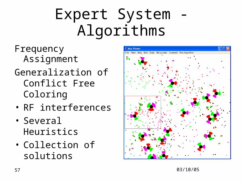
Expert System - Algorithms
Frequency Assignment
Generalization of Conflict Free Coloring
• RF interferences• Several Heuristics • Collection of solutions
03/10/0558
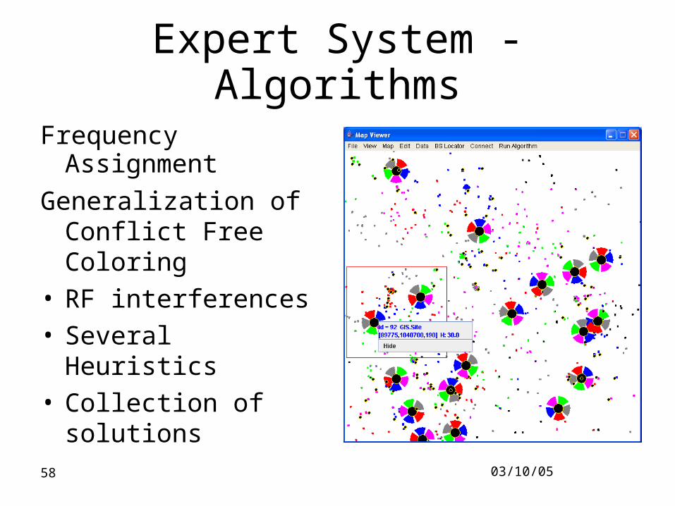
Expert System - Algorithms
Frequency Assignment
Generalization of Conflict Free Coloring
• RF interferences• Several Heuristics • Collection of solutions
03/10/0559
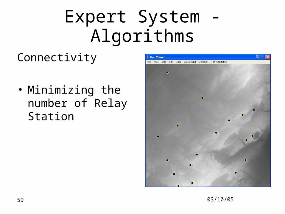
Expert System - Algorithms
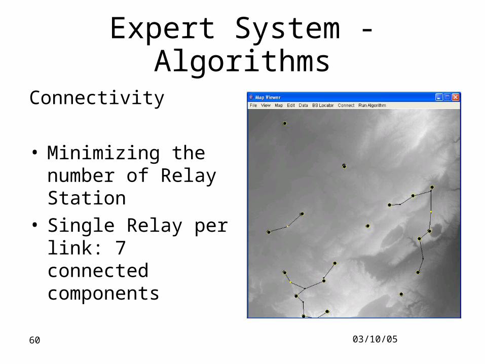
Connectivity
• Minimizing the number of Relay Station
03/10/0560
Expert System - Algorithms
Connectivity
• Minimizing the number of Relay Station
• Single Relay per link: 7 connected components

03/10/0561
Expert System - Algorithms
Connectivity
• Minimizing the number of Relay Station
• Three Relays per link: a single connected component
03/10/0562
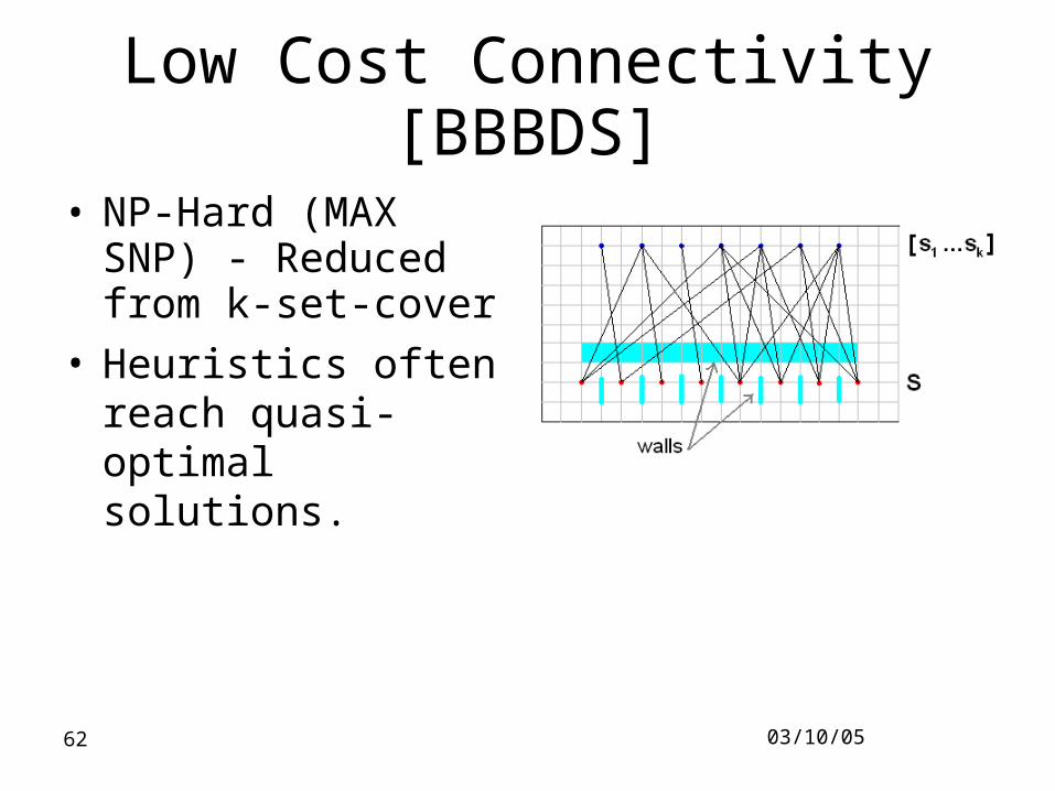
Low Cost Connectivity [BBBDS]
• NP-Hard (MAX SNP) - Reduced from k-set-cover
• Heuristics often reach quasi-optimal solutions.
03/10/0563
Low Cost Connectivity
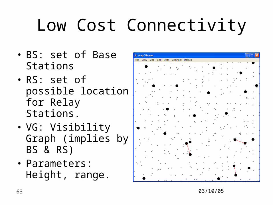
• BS: set of Base Stations
• RS: set of possible location for Relay Stations.
• VG: Visibility Graph (implies by BS & RS)
• Parameters: Height, range.
03/10/0564
Low Cost Connectivity
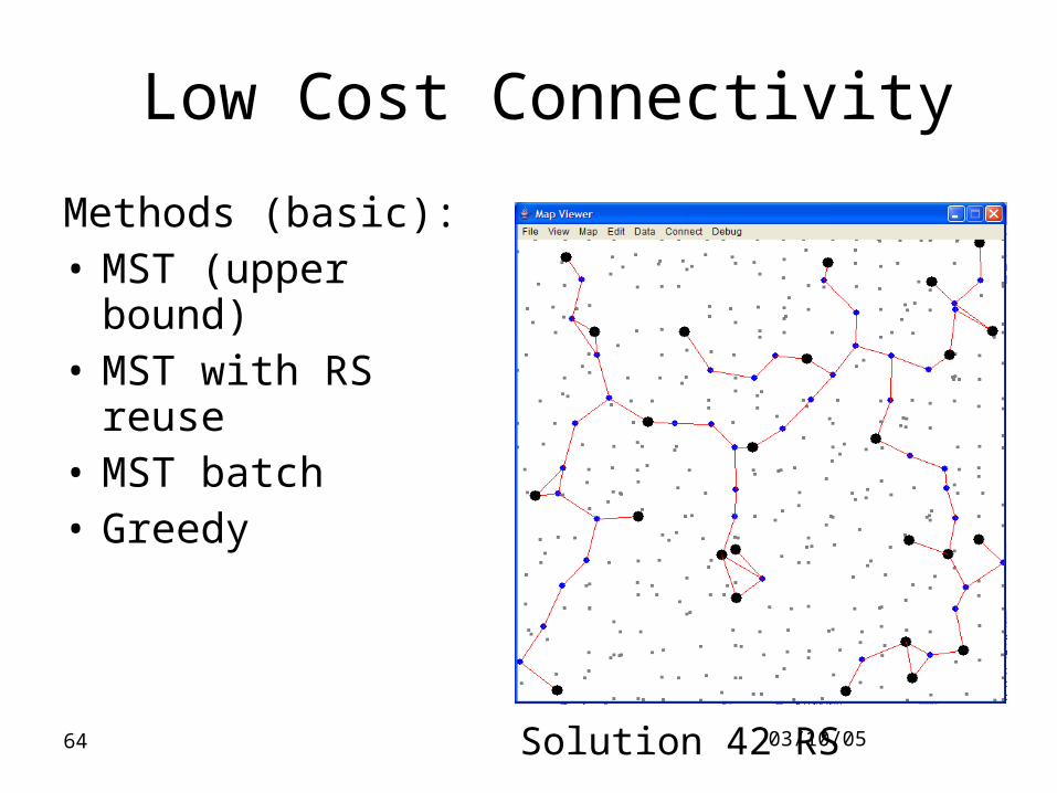
Methods (basic):• MST (upper bound)• MST with RS reuse• MST batch• Greedy
Solution 42 RS
03/10/0565
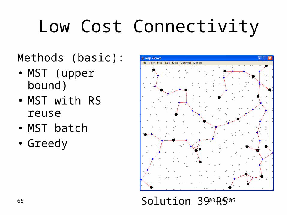
Low Cost Connectivity
Methods (basic):• MST (upper bound)• MST with RS reuse• MST batch• Greedy
Solution 39 RS
03/10/0566
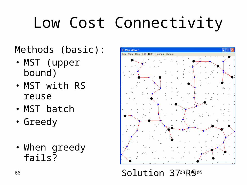
Low Cost Connectivity
Methods (basic):• MST (upper bound)• MST with RS reuse• MST batch• Greedy
• When greedy fails?
Solution 37 RS
03/10/0567
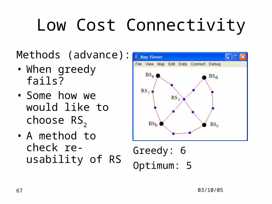
Low Cost Connectivity
Methods (advance):• When greedy fails?• Some how we would
like to choose RS2
• A method to check re-usability of RS
Greedy: 6
Optimum: 5
03/10/0568
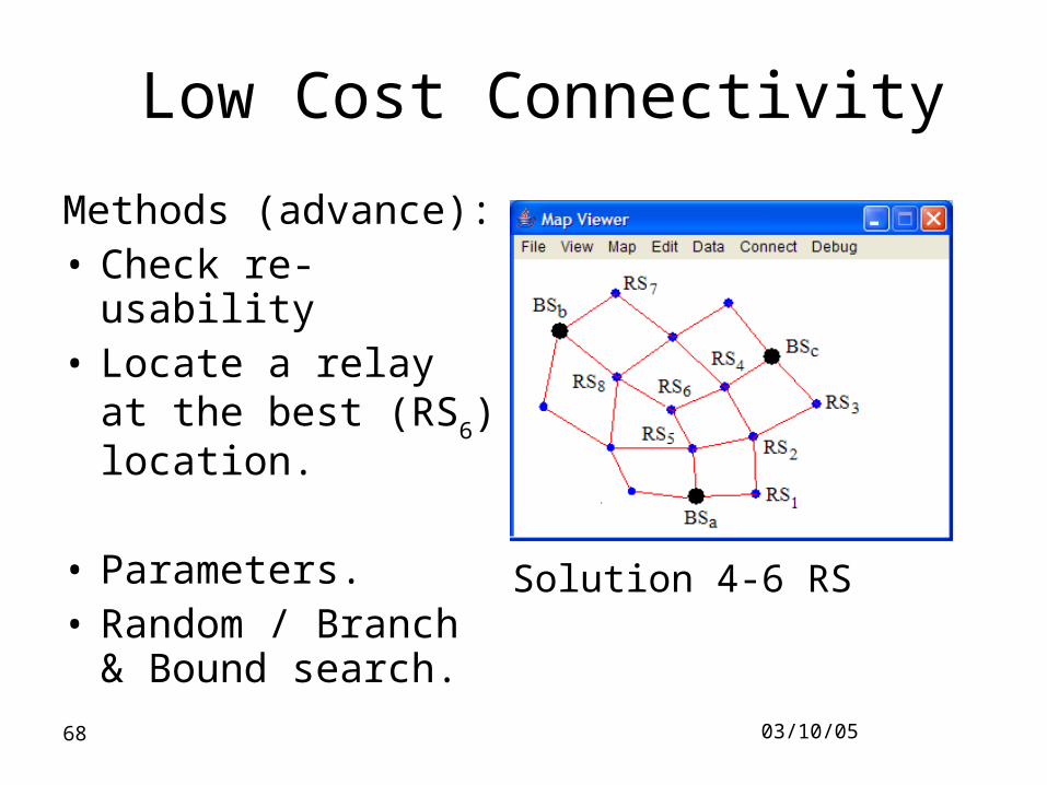
Low Cost Connectivity
Methods (advance):• Check re-usability• Locate a relay at the
best (RS6) location.
• Parameters.• Random / Branch &
Bound search. Solution 4-6 RS
03/10/0569
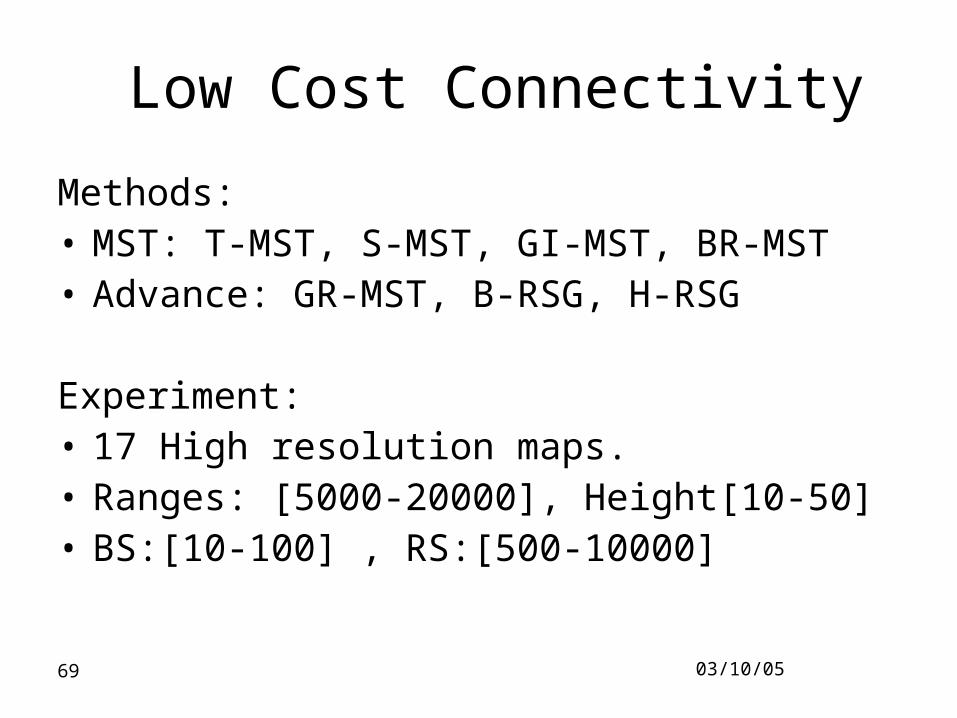
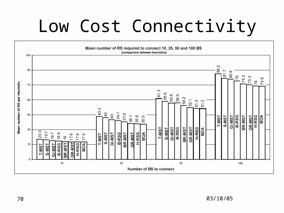
Low Cost Connectivity
Methods:• MST: T-MST, S-MST, GI-MST, BR-MST • Advance: GR-MST, B-RSG, H-RSG
Experiment: • 17 High resolution maps.• Ranges: [5000-20000], Height[10-50]• BS:[10-100] , RS:[500-10000]
03/10/0570
Low Cost Connectivity