Embed Size (px)
Citation preview
February 2014
Working paper
ROCK AROUND THE CLOCK: AN AGENT-BASED MODEL OF LOW-
AND HIGH-FREQUENCY TRADING
Sandrine Jacob Leal CEREFIGE - ICN Business School (Nancy-Metz) France - GREDEG
Mauro Napoletano
OFCE, SKEMA Business School, Scuola Superiore Sant’Anna
Andrea Roventini Università di Verona – Scuola Superiore Sant’Anna- OFCE
Giorgio Fagiolo
Scuola Superiore Sant’Anna
2014
-03
Rock around the Clock: An Agent-Based Model of Low-
and High-Frequency Trading
Sandrine Jacob Leal∗ Mauro Napoletano† Andrea Roventini‡
Giorgio Fagiolo§
January 31, 2014
Abstract
We build an agent-based model to study how the interplay between low- and high-frequency trading affects asset price dynamics. Our main goal is to investigatewhether high-frequency trading exacerbates market volatility and generates flashcrashes. In the model, low-frequency agents adopt trading rules based on chrono-logical time and can switch between fundamentalist and chartist strategies. Onthe contrary, high-frequency traders activation is event-driven and depends on pricefluctuations. High-frequency traders use directional strategies to exploit market in-formation produced by low-frequency traders. Monte-Carlo simulations reveal thatthe model replicates the main stylized facts of financial markets. Furthermore, wefind that the presence of high-frequency trading increases market volatility and playsa fundamental role in the generation of flash crashes. The emergence of flash crashesis explained by two salient characteristics of high-frequency traders, i.e., their abilityto i) generate high bid-ask spreads and ii) synchronize on the sell side of the limitorder book. Finally, we find that higher rates of order cancellation by high-frequencytraders increase the incidence of flash crashes but reduce their duration.
Keywords: Agent-based models, Limit order book, High-frequency trading, Low-frequency trading, Flash crashes, Market volatility
JEL codes: G12, G01, C63
∗Corresponding author. CEREFIGE - ICN Business School (Nancy-Metz) France - GREDEG. Ad-dress: ICN Business School (Nancy-Metz) 13, rue Michel Ney, 54000 Nancy (France). Tel:+33 383173776.Fax:+33 383173080. E-mail address: [email protected]†OFCE, Skema Business School, Sophia-Antipolis (France), and Scuola Superiore Sant’Anna, Pisa
(Italy). E-mail address: [email protected]‡Universita di Verona (Italy); Scuola Superiore Sant’Anna, Pisa (Italy), and OFCE, Sophia-Antipolis
(France). E-mail address: [email protected]§Scuola Superiore Sant’Anna, Pisa (Italy). E-mail address: [email protected]
1
1 Introduction
This paper builds an agent-based model to study how high-frequency trading affects asset
price volatility as well as the occurrence and the duration of flash crashes in financial
markets.
The increased frequency and severity of flash crashes and the high volatility of prices
observed in financial time series have recently been associated to the rising importance
of high-frequency trading (see, e.g., Sornette and Von der Becke, 2011, and further refer-
ences therein). However, the debate in the literature about the benefits and costs of high
frequency trading (HFT henceforth) has not been settled yet. On the one hand, some
works stress that high-frequency traders may play the role of modern market-makers,
providing an almost continuous flow of liquidity (Menkveld, 2013). Moreover, HFT re-
duces transaction costs and favors price discovery and market efficiency by strengthening
the links between different markets (Brogaard, 2010). On the other hand, many empir-
ical and theoretical studies raise concerns about the threatening effects of HFT on the
dynamics of financial markets. In particular, HFT may lead to more frequent periods
of illiquidity, possibly leading to the emergence of flash crashes (Kirilenko et al, 2011).
Furthermore, HFT may exacerbate market volatility (Zhang, 2010; Hanson, 2011) and
negatively affect market efficiency (Wah and Wellman, 2013).
This work contributes to the current debate on the impact of HFT on asset price
dynamics by developing an agent-based model of a limit-order book (LOB) market1
wherein heterogeneous high-frequency (HF) traders interact with low-frequency (LF)
ones. Our main goal is to study whether HFT helps to explain the emergence of flash
crashes and more generally periods of higher volatility in financial markets. Moreover, we
want to shed some light on which distinct features of HFT are relevant in the generation
of flash crashes and affect the process of price-recovery after a crash.
In the model, LF traders can switch between fundamentalist and chartist strategies
according to their profitability. HF traders adopt directional strategies that exploit the
price and volume-size information produced by LF traders (cf. SEC, 2010; Aloud et al,
2011). Moreover, in line with empirical evidence on HFT (see e.g., Easley et al, 2012),
LF trading strategies are based on chronological time, whereas those of HF traders are
framed in event time.2 Consequently, LF agents, who trade at exogenous and constant
1See, for instance, Farmer et al (2005) and Slanina (2008) for detailed studies of the effect of limit-order book models on market dynamics.
2As noted by Easley et al (2012), HFT requires the adoption of algorithmic trading implementedthrough computers which natively operate on internal event-based clocks. Hence, the study of HFTcannot be reduced to its higher speed only, but it should take into account also the associated new
2
frequency, co-evolve with HF agents, whose participation in the market is endogenously
triggered by price fluctuations. Finally, consistent with empirical evidence (see Kirilenko
et al, 2011), HF traders face limits in the accumulation of open positions.
So far, the few existing agent-based models dealing with HFT have mainly treated HF
as zero-intelligence agents with an exogenously-given trading frequency (e.g., Bartolozzi,
2010; Hanson, 2011). However, only few attempts have been made to account for the
interplay between HF and LF traders (see, for instance, Paddrik et al, 2011; Aloud
et al, 2013; Wah and Wellman, 2013). We improve upon this literature along several
dimensions. First, we depart from the zero-intelligent framework by considering HF
traders who hold event-based trading-activation rules, and place orders according to
observed market volumes, constantly exploiting the information provided by LF traders.
Second, we explicitly account for the interplay among many HF and LF traders. Finally,
we perform a deeper investigation of the characteristics of HFT that generate price
downturns, and of the factors explaining the fast price-recovery one typically observes
after flash crashes.
We study the model in two different scenarios. In the first scenario (“only-LFT”
case), only LF agents trade with each other. In the second scenario (our baseline),
both LF and HF traders co-exist in the market. The comparison of the simulation
results generated from these two scenarios allows us to assess the contribution of high-
frequency trading to financial market volatility and to the emergence of flash crashes.
In addition, we perform extensive Monte-Carlo experiments wherein we vary the rate of
HF traders’ order cancellation in order to study its impact on asset price dynamics.
Monte-Carlo simulations reveal that the model replicates the main stylized facts of
financial markets (i.e., zero autocorrelation of returns, volatility clustering, fat-tailed
returns distribution) in both scenarios. However, we observe flash crashes together with
high price volatility only when HF agents are present in the market. Moreover, we find
that the emergence of flash crashes is explained by two salient characteristics of HFT,
namely the ability of HF traders (i) to grasp market liquidity leading to high bid-ask
spreads in the LOB; (ii) to synchronize on the sell-side of the limit order book, triggered
by their event-based strategies. Furthermore, we observe that sharp drops in prices
coincide with the contemporaneous concentration of LF traders’ orders on the buy-side
of the book. In addition, we find that the fast recoveries observed after price crashes
result from both a more equal distribution of HF agents on both sides of the book and
a lower persistence of HF agents’ orders in the LOB. Finally, we show that HF agents’
order cancellations have an ambiguous effect on price fluctuations. On the one hand,
trading paradigm. See also Aloud et al (2013) for a modeling attempt in the same direction.
3
high rates of order cancellation imply higher volatility and more frequent flash crashes.
On the other hand, they also lead to faster price-recoveries, which reduce the duration
of flash crashes.
Overall, our results validate the hypothesis that HFT exacerbates asset price volatil-
ity, generates flash crashes and periods of market illiquidity (as measured by large bid-
ask spreads). At the same time, consistent with the recent academic and public debates
about HFT, our findings highlight the complex effects of HF traders’ order cancellation
on price dynamics.3
The rest of the paper is organized as follows. Section 2 describes the model. In
Section 3, we present and discuss the simulation results. Finally, Section 4 concludes.
2 The Model
We model a stock market populated by heterogeneous, boundedly-rational traders.
Agents trade an asset for T periods and transactions are executed through a limit-order
book (LOB) where the type, the size and the price of all agents’ orders are stored.4
Agents are classified in two groups according to their trading frequency, i.e., the av-
erage amount of time elapsed between two order placements. More specifically, the
market is populated by NL low-frequency (LF) and NH high-frequency (HF) traders
(N = NL + NH). Note that, even if the number of agents in the two groups is kept
fixed over the simulations, the proportion of low- and high-frequency traders changes
over time as some agents may not be active in each trading session. Moreover, agents in
the two groups are different not only in terms of trading frequencies, but also in terms
of strategies and activation rules. A detailed description of the behavior of LF and HF
traders is provided in Sections 2.2 and 2.3. We first present the timeline of events of a
representative trading session (cf. Section 2.1).
2.1 The Timeline of Events
At the beginning of each trading session t, active LF and HF agents know the past closing
price as well as the past and current fundamental values According to the foregoing
3See Hasbrouck and Saar (2009) for an empirical investigation of the importance of order cancellationin current financial markets and of its determinants. See, among others, the articles in Economist (2012);Brundsen (2012); Patterson and Ackerman (2012) for the importance of HFT order cancellation in thepublic debate.
4See Maslov (2000); Zovko and Farmer (2002); Farmer et al (2005); Avellaneda and Stoikov (2008);Pellizzari and Westerhoff (2009); Bartolozzi (2010); Cvitanic and Kirilenko (2010). For a detailed studyof the statistical properties of the limit order book cf. Bouchaud et al (2002); Luckock (2003); Smithet al (2003).
4
information set, in each session t, trading proceeds as follows:
1. Active LF traders submit their buy/sell orders to the LOB market, specifying their
size and limit price.
2. Knowing the orders of LF traders, active HF agents start trading sequentially and
submit their buy/sell orders. The size and the price of their orders are also listed
in the LOB.
3. LF and HF agents’ orders are matched and executed5 according to their price and
then arrival time. Unexecuted orders rest in the LOB for the next trading session.
4. At the end of the trading session, the closing price (Pt) is determined. The closing
price is the maximum price of all executed transactions in the session.
5. Given Pt, all agents compute their profits and LF agents update their strategy for
the next trading session (see Section 2.2 below).
2.2 Low-Frequency Traders
In the market, there are i = 1, . . . , NL low-frequency agents who take short or long posi-
tions on the traded asset. The trading frequency of LF agents is based on chronological
time, i.e. it is exogenous and constant over time. In particular, LF agents’ trading speed
is drawn from a truncated exponential distribution with mean θ and bounded between
θmin and θmax minutes.
In line with most heterogeneous-agent models of financial markets, LF agents deter-
mine the quantities bought or sold (i.e., their orders) according to either a fundamentalist
or a chartist (trend-following) strategy.6 More precisely, given the last closing price Pt−1,
orders under the chartist strategy (Dci,t) are determined as follows:
Dci,t = αc(Pt−1 − Pt−2) + εct , (1)
where 0 < αc < 1 and εct is an i.i.d. Gaussian stochastic variable with zero mean and
σc standard deviation. If a LF agent follows a fundamentalist strategy, her orders (Dfi,t)
are equal to:
Dfi,t = αf (Ft − Pt−1) + εft , (2)
5The price of an executed contract is the average between the matched bid and ask quotes.6See, e.g., Chiarella (1992); Lux (1995); Lux and Marchesi (2000); Farmer (2002); Chiarella and He
(2003); Hommes et al (2005); Chiarella et al (2006); Westerhoff (2008).
5
where 0 < αf < 1 and εft is an i.i.d. normal random variable with zero mean and
σf standard deviation. The fundamental value of the asset Ft evolves according to a
geometric random walk:
Ft = Ft−1(1 + δ)(1 + yt), (3)
with i.i.d. yt ∼ N(0, σy) and a constant term δ > 0. After γL periods, unexecuted orders
expire, i.e. they are automatically withdrawn from the LOB. Finally, the limit-order
price of each LF trader is determined by:
Pi,t = Pt−1(1 + δ)(1 + zi,t), (4)
where zi,t measures the number of ticks away from the last closing price Pt−1 and it is
drawn from a Gaussian distribution with zero mean and σz standard deviation.
In each period, low-frequency traders can switch their strategies according to their
profitability. At the end of each trading session t, once the closing price Pt is determined,
LF agent i computes her profits (πsti,t) under chartist (st = c) and fundamentalist (st = f)
trading strategies as follows:
πsti,t = (Pt − Pi,t)Dsti,t. (5)
Following Brock and Hommes (1998), Westerhoff (2008), and Pellizzari and Westerhoff
(2009), the probability that a LF trader will follow a chartist rule in the next period
(Φci,t) is given by:
Φci,t =
eπci,t/ζ
eπci,t/ζ + eπ
fi,t/ζ
, (6)
with a positive intensity of switching parameter ζ. Accordingly, the probability that LF
agent i will use a fundamentalist strategy is equal to Φfi,t = 1 − Φc
i,t.
2.3 High-Frequency Traders
As mentioned above, the market is also populated by j = 1, . . . , NH high-frequency
agents who buy and sell the asset.7
HF agents differ from LF ones not only in terms of trade speed, but also in terms of
activation and trading rules. In particular, contrary to LF strategies, which are based
on chronological time, the algorithmic trading underlying the implementation of HFT
naturally leads HF agents to adopt trading rules framed in event time (see e.g., Easley
7We assume that NH < NL. The proportion of HF agents vis-a-vis LF ones is in line with empiricalevidence (Kirilenko et al, 2011; Paddrik et al, 2011).
6
et al, 2012).8 More precisely, we assume that the activation of HF agents depends on
the extent of price fluctuations observed in the market. As a consequence, HF agents’
trading speed is endogenous. Each HF trader has a fixed price threshold ∆xj , drawn from
a uniform distribution with support bounded between ηmin and ηmax. This determines
whether she will participate or not in the trading session t:9∣∣∣∣∣ Pt−1 − Pt−2Pt−2
∣∣∣∣∣ > ∆xj . (7)
Active HF agents submit buy or sell limit orders with equal probability p = 0.5 (Maslov,
2000; Farmer et al, 2005).
Furthermore, HF traders adopt directional strategies that try to profit from the
anticipation of price movements (see SEC, 2010; Aloud et al, 2011). To do this, HF
agents exploit the price and order information released by LF agents.
First, HF traders determine their buy (sell) order size, Dj,t, according to the volumes
available in the opposite side of the LOB. More specifically, HF traders’ order size is
drawn from a truncated Poisson distribution whose mean depends on volumes available
in the sell(buy)-side of the LOB if the order is a buy (sell) order.10 As HF traders adjust
the volumes of their orders to the ones available in the LOB, they manage to absorb LF
agents’ orders.
Second, in each trading session t, HF agents trade near the best ask (P askt ) and
bid (P bidt ) prices available in the LOB (see e.g., Paddrik et al, 2011). This assumption
is consistent with empirical evidence on HF agents’ behavior which suggest that most
of their orders are placed very close to the last best prices (CFTC and SEC, 2010).
Accordingly, HF buyers and sellers’ limit prices are formed as follows:
Pj,t = P askt (1 + κj) Pj,t = P bidt (1 − κj), (8)
where κj is drawn from a uniform distribution with support (κmin, κmax).
A key characteristic of empirically-observed high-frequency trading is the high order
8On the case for moving away from chronological time in modeling financial series see Mandelbrotand Taylor (1967); Clark (1973); Ane and Geman (2000).
9See Aloud et al (2013) for a similar attempt in this direction.10In the computation of this mean, the relevant market volumes are weighted by the parameter 0 <
λ < 1. This link between market volumes and HF traders’ order size is motivated by the empiricalevidence which suggests that HF traders typically submit large orders (Kirilenko et al, 2011). Moreover,empirical works also indicate that HF traders do not accumulate large net positions. Thus, we introducetwo additional constraints to HF order size. First, HF traders’ net position is bounded between +/-3,000.Second, HF traders’ buy (sell) orders are smaller than one quarter of the total volume present in the sell(buy) side of the LOB (see, for instance, Kirilenko et al, 2011; Bartolozzi, 2010; Paddrik et al, 2011).
7
cancellation rate (CFTC and SEC, 2010; Kirilenko et al, 2011). We introduce such a
feature in the model by assuming that HF agents’ unexecuted orders are automatically
removed from the LOB after a period of time γH , which is shorter than LF agents’ one,
i.e. γH < γL. Finally, at the end of each trading session, HF traders’ profits (πj,t) are
computed as follows:11
πj,t = (Pt − Pj,t)Dj,t. (9)
where Dj,t is the HF agent’s order size, Pj,t is her limit price and Pt is the market closing
price.
3 Simulation Results
We investigate the properties of the model presented in the previous section via extensive
Monte-Carlo simulations. More precisely, we carry out MC = 50 Monte-Carlo iterations,
each one composed of T = 1, 200 trading sessions using the baseline parametrization,
described in Table 4. As a first step in our analysis of simulation results, we check
whether the model is able to account for the main stylized facts of financial markets (see
Section 3.1). We then assess whether the model can generate flash crashes characterized
by empirical properties close to the ones observed in real data (cf. Section 3.2) and
we investigate the determinants of flash crashes (cf. Section 3.3). Finally, we study
post flash-crash recoveries by investigating the consequences of different degrees of HF
traders’ order cancellation on model dynamics (see Section 3.4).
3.1 Stylized Facts of Financial Markets
How does the model fare in terms of its ability to replicate the main statistical properties
of financial markets? First, in line with the empirical evidence of zero autocorrelation
detected in price returns (e.g., Fama, 1970; Pagan, 1996; Chakraborti et al, 2011, and
references therein), we find that model-generated autocorrelation values of price-returns
(calculated as logarithmic differences) do not reveal any significant pattern and are
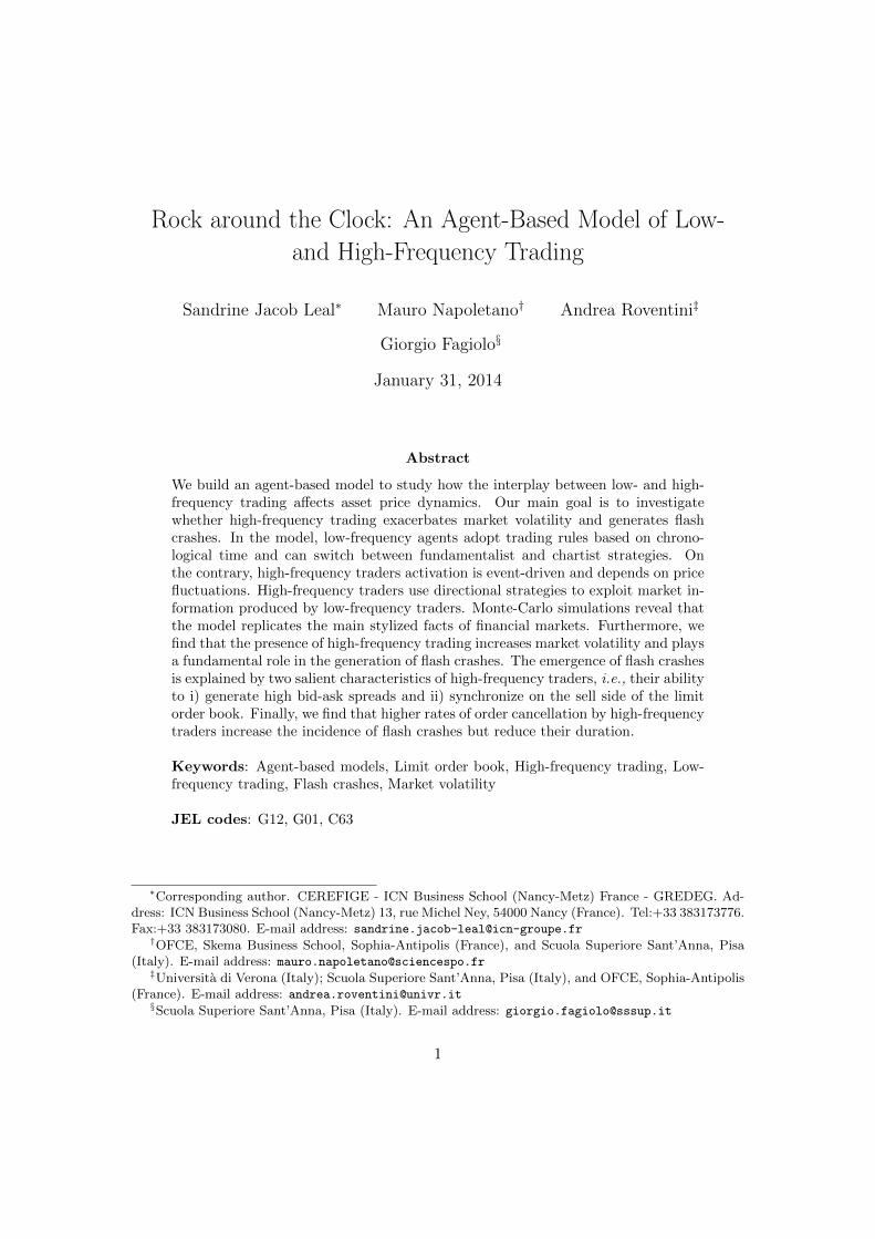
always not significantly different from zero (see the box-whisker plots in Figure 1).12
Moreover, in contrast to price returns, the autocorrelation functions of both absolute
11Simulation exercises in the baseline scenario reveal that the strategies adopted by HF traders areable to generate positive profits, thus justifying their adoption by HF agents in the model. In particular,simulation results reveal that the distribution of HF traders’ profits is skewed to the right and has apositive mean.
12More precisely, the confidence interval of the values at each lag (measured by the extent of thewhiskers) always includes the zero. Notice that each whiskers’ length in the plot corresponds to 99.3%data coverage under the assumption that autocorrelation values are drawn from a Normal distribution.
8
1 2 3 4 5 6 7 8 9 10 11 12 13 14 15 16 17 18 19 20−0.2
−0.15
−0.1
−0.05
0
0.05
0.1
0.15
0.2
Lags
Au
toco
rre
latio
n V
alu
es
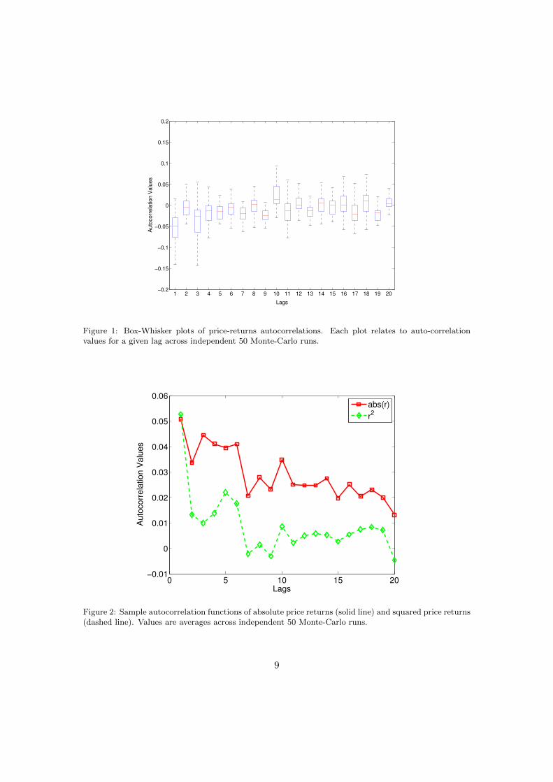
Figure 1: Box-Whisker plots of price-returns autocorrelations. Each plot relates to auto-correlationvalues for a given lag across independent 50 Monte-Carlo runs.
0 5 10 15 20−0.01
0
0.01
0.02
0.03
0.04
0.05
0.06
Au
toco
rre
latio
n V
alu
es
Lags
abs(r)
r2
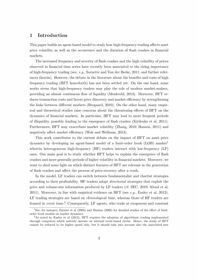
Figure 2: Sample autocorrelation functions of absolute price returns (solid line) and squared price returns(dashed line). Values are averages across independent 50 Monte-Carlo runs.
9
−0.4 −0.3 −0.2 −0.1 0 0.1 0.2 0.3 0.410
−3
10−2
10−1
100
101
102
Price Returns
f(x)
Simulated Returns
Normal Distribution
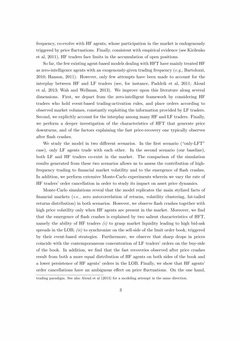
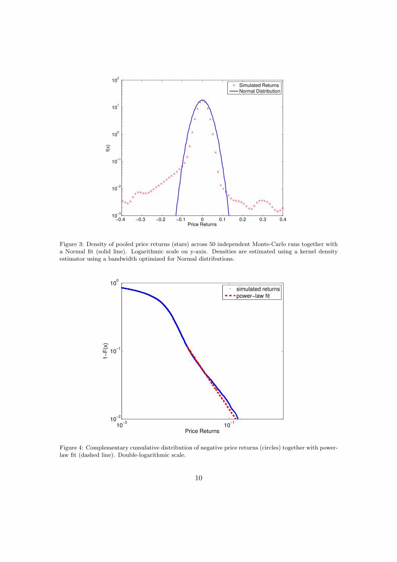
Figure 3: Density of pooled price returns (stars) across 50 independent Monte-Carlo runs together witha Normal fit (solid line). Logarithmic scale on y-axis. Densities are estimated using a kernel densityestimator using a bandwidth optimized for Normal distributions.
10−3
10−1
10−2
10−1
100
1−
F(x
)
Price Returns
simulated returns
power−law fit
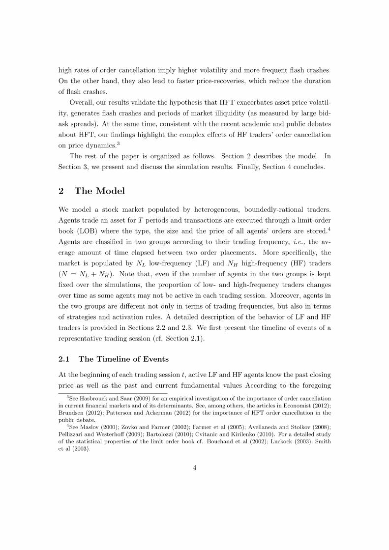
Figure 4: Complementary cumulative distribution of negative price returns (circles) together with power-law fit (dashed line). Double-logarithmic scale.
10
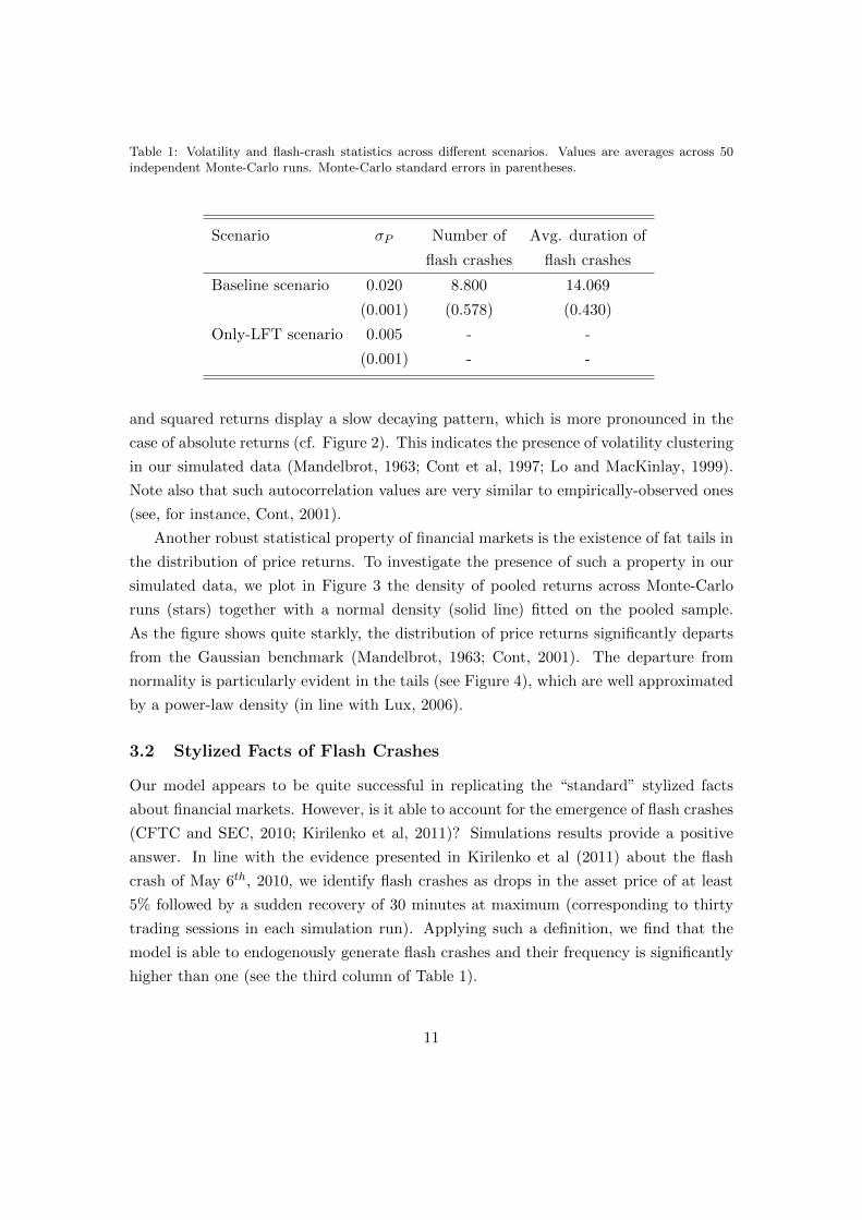
Table 1: Volatility and flash-crash statistics across different scenarios. Values are averages across 50independent Monte-Carlo runs. Monte-Carlo standard errors in parentheses.
Scenario σP Number of Avg. duration of
flash crashes flash crashes
Baseline scenario 0.020 8.800 14.069
(0.001) (0.578) (0.430)
Only-LFT scenario 0.005 - -
(0.001) - -
and squared returns display a slow decaying pattern, which is more pronounced in the
case of absolute returns (cf. Figure 2). This indicates the presence of volatility clustering
in our simulated data (Mandelbrot, 1963; Cont et al, 1997; Lo and MacKinlay, 1999).
Note also that such autocorrelation values are very similar to empirically-observed ones
(see, for instance, Cont, 2001).
Another robust statistical property of financial markets is the existence of fat tails in
the distribution of price returns. To investigate the presence of such a property in our
simulated data, we plot in Figure 3 the density of pooled returns across Monte-Carlo
runs (stars) together with a normal density (solid line) fitted on the pooled sample.
As the figure shows quite starkly, the distribution of price returns significantly departs
from the Gaussian benchmark (Mandelbrot, 1963; Cont, 2001). The departure from
normality is particularly evident in the tails (see Figure 4), which are well approximated
by a power-law density (in line with Lux, 2006).
3.2 Stylized Facts of Flash Crashes
Our model appears to be quite successful in replicating the “standard” stylized facts
about financial markets. However, is it able to account for the emergence of flash crashes
(CFTC and SEC, 2010; Kirilenko et al, 2011)? Simulations results provide a positive
answer. In line with the evidence presented in Kirilenko et al (2011) about the flash
crash of May 6th, 2010, we identify flash crashes as drops in the asset price of at least
5% followed by a sudden recovery of 30 minutes at maximum (corresponding to thirty
trading sessions in each simulation run). Applying such a definition, we find that the
model is able to endogenously generate flash crashes and their frequency is significantly
higher than one (see the third column of Table 1).
11
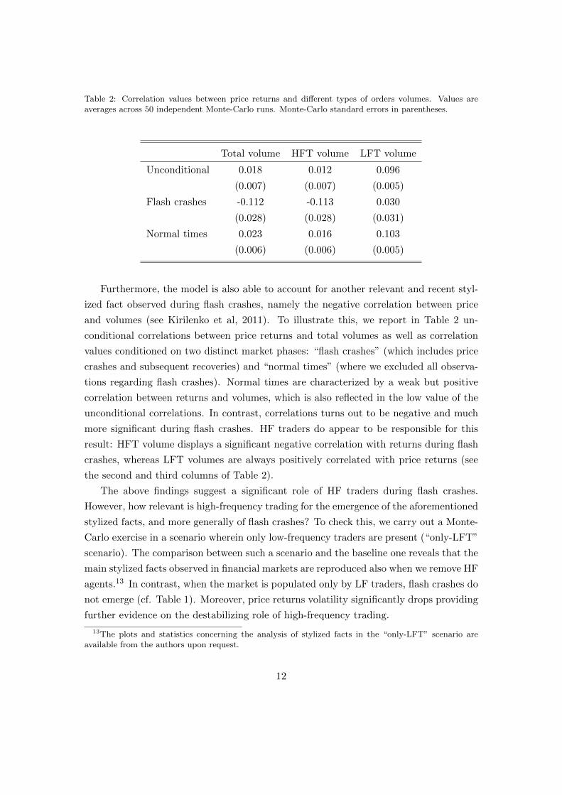
Table 2: Correlation values between price returns and different types of orders volumes. Values areaverages across 50 independent Monte-Carlo runs. Monte-Carlo standard errors in parentheses.
Total volume HFT volume LFT volume
Unconditional 0.018 0.012 0.096
(0.007) (0.007) (0.005)
Flash crashes -0.112 -0.113 0.030
(0.028) (0.028) (0.031)
Normal times 0.023 0.016 0.103
(0.006) (0.006) (0.005)
Furthermore, the model is also able to account for another relevant and recent styl-
ized fact observed during flash crashes, namely the negative correlation between price
and volumes (see Kirilenko et al, 2011). To illustrate this, we report in Table 2 un-
conditional correlations between price returns and total volumes as well as correlation
values conditioned on two distinct market phases: “flash crashes” (which includes price
crashes and subsequent recoveries) and “normal times” (where we excluded all observa-
tions regarding flash crashes). Normal times are characterized by a weak but positive
correlation between returns and volumes, which is also reflected in the low value of the
unconditional correlations. In contrast, correlations turns out to be negative and much
more significant during flash crashes. HF traders do appear to be responsible for this
result: HFT volume displays a significant negative correlation with returns during flash
crashes, whereas LFT volumes are always positively correlated with price returns (see
the second and third columns of Table 2).
The above findings suggest a significant role of HF traders during flash crashes.
However, how relevant is high-frequency trading for the emergence of the aforementioned
stylized facts, and more generally of flash crashes? To check this, we carry out a Monte-
Carlo exercise in a scenario wherein only low-frequency traders are present (“only-LFT”
scenario). The comparison between such a scenario and the baseline one reveals that the
main stylized facts observed in financial markets are reproduced also when we remove HF
agents.13 In contrast, when the market is populated only by LF traders, flash crashes do
not emerge (cf. Table 1). Moreover, price returns volatility significantly drops providing
further evidence on the destabilizing role of high-frequency trading.
13The plots and statistics concerning the analysis of stylized facts in the “only-LFT” scenario areavailable from the authors upon request.
12
200 300 400 500 600 700 800 900 1000 1100 1200120
140
160
180
200
Time
Price
200 300 400 500 600 700 800 900 1000 1100 12000
10
20
30
40
Bid
−A
sk S
pre
ad
Price
Bid−Ask Spread
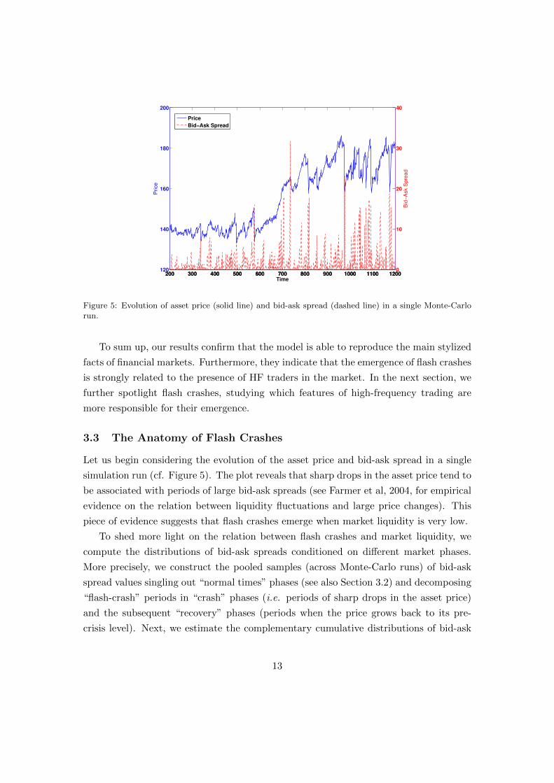
Figure 5: Evolution of asset price (solid line) and bid-ask spread (dashed line) in a single Monte-Carlorun.
To sum up, our results confirm that the model is able to reproduce the main stylized
facts of financial markets. Furthermore, they indicate that the emergence of flash crashes
is strongly related to the presence of HF traders in the market. In the next section, we
further spotlight flash crashes, studying which features of high-frequency trading are
more responsible for their emergence.
3.3 The Anatomy of Flash Crashes
Let us begin considering the evolution of the asset price and bid-ask spread in a single
simulation run (cf. Figure 5). The plot reveals that sharp drops in the asset price tend to
be associated with periods of large bid-ask spreads (see Farmer et al, 2004, for empirical
evidence on the relation between liquidity fluctuations and large price changes). This
piece of evidence suggests that flash crashes emerge when market liquidity is very low.
To shed more light on the relation between flash crashes and market liquidity, we
compute the distributions of bid-ask spreads conditioned on different market phases.
More precisely, we construct the pooled samples (across Monte-Carlo runs) of bid-ask
spread values singling out “normal times” phases (see also Section 3.2) and decomposing
“flash-crash” periods in “crash” phases (i.e. periods of sharp drops in the asset price)
and the subsequent “recovery” phases (periods when the price grows back to its pre-
crisis level). Next, we estimate the complementary cumulative distributions of bid-ask
13
0 20 40 60 80 1000
0.1
0.2
0.3
0.4
0.5
0.6
0.7
0.8
0.9
1
Bid Ask Spread Values
1−
F(x
)
normal times
crash
recovery
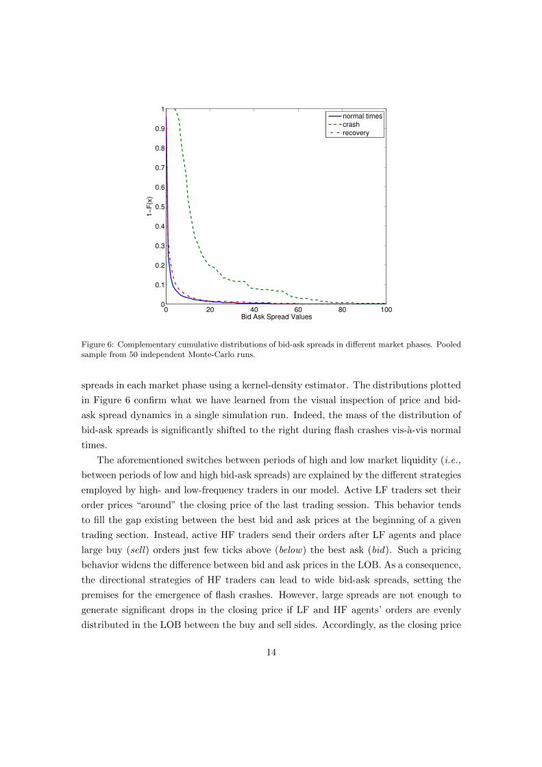
Figure 6: Complementary cumulative distributions of bid-ask spreads in different market phases. Pooledsample from 50 independent Monte-Carlo runs.
spreads in each market phase using a kernel-density estimator. The distributions plotted
in Figure 6 confirm what we have learned from the visual inspection of price and bid-
ask spread dynamics in a single simulation run. Indeed, the mass of the distribution of
bid-ask spreads is significantly shifted to the right during flash crashes vis-a-vis normal
times.
The aforementioned switches between periods of high and low market liquidity (i.e.,
between periods of low and high bid-ask spreads) are explained by the different strategies
employed by high- and low-frequency traders in our model. Active LF traders set their
order prices “around” the closing price of the last trading session. This behavior tends
to fill the gap existing between the best bid and ask prices at the beginning of a given
trading section. Instead, active HF traders send their orders after LF agents and place
large buy (sell) orders just few ticks above (below) the best ask (bid). Such a pricing
behavior widens the difference between bid and ask prices in the LOB. As a consequence,
the directional strategies of HF traders can lead to wide bid-ask spreads, setting the
premises for the emergence of flash crashes. However, large spreads are not enough to
generate significant drops in the closing price if LF and HF agents’ orders are evenly
distributed in the LOB between the buy and sell sides. Accordingly, as the closing price
14
is the maximum price of all executed transactions in the book, an even distribution of
orders should lead to small fluctuations in the closing price. In contrast, extreme price
fluctuations require concentration of orders on one side of the book.
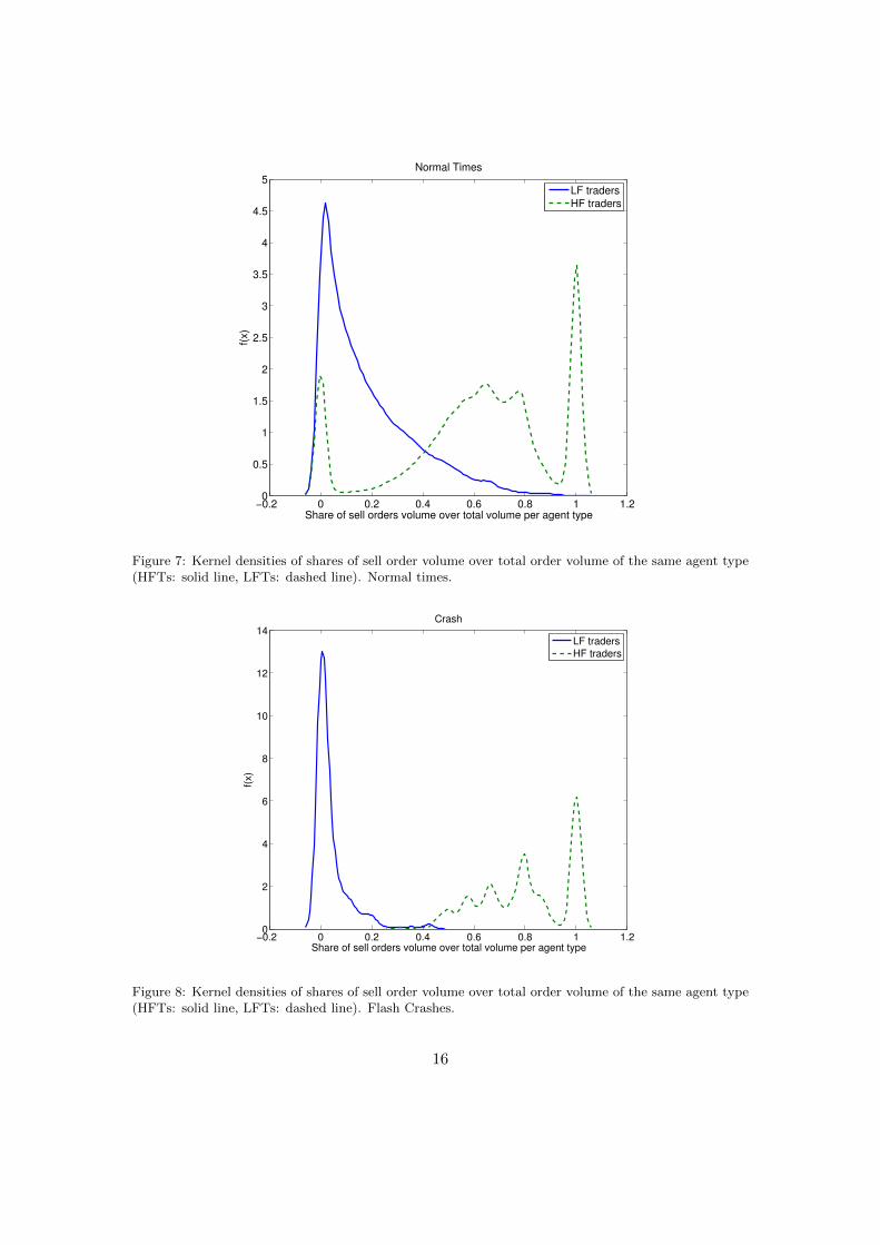
To further explore such conjecture, we analyze the distributions of shares of sell
order volumes in the book made by each type of agent (HF or LF traders) over the total
volume within the same category. This ratio captures the concentration of the orders
on the sell side of the LOB disaggregated for agents’ type. In particular, the more the
sell concentration ratio is close to one, the more a given category of agents (e.g., HF
traders) is filling the LOB with sell orders. Figures 7 and 8 compare kernel densities of
the foregoing sell concentration ratios for HF and LF agents in normal times and crashes,
respectively. Let us start examining the latter. First, Figure 8 shows that during crashes
the supports of the LF and HF traders’ distributions do not overlap. This hints to a
very different behavior of LF and HF agents during flash crashes. Second, during crash
times, LF and HF traders’ orders are concentrated on opposite sides of the LOB. More
specifically, the mass of the distribution of LF agents’ orders is concentrated on the buy
side of the book, whereas the mass of the HF traders’ distribution is found on very high
values of the sell concentration ratio (see Figure 8). These extreme behaviors are not
observed during normal times (cf. Figure 7). Indeed, in tranquil market phases, the
supports of the LFT and HFT densities overlap and they encompass the whole support
of the sell concentration statistic.
We further study the above differences in order behavior, analyzing the complemen-
tary cumulative distributions of the sell concentration statistic for the same type of
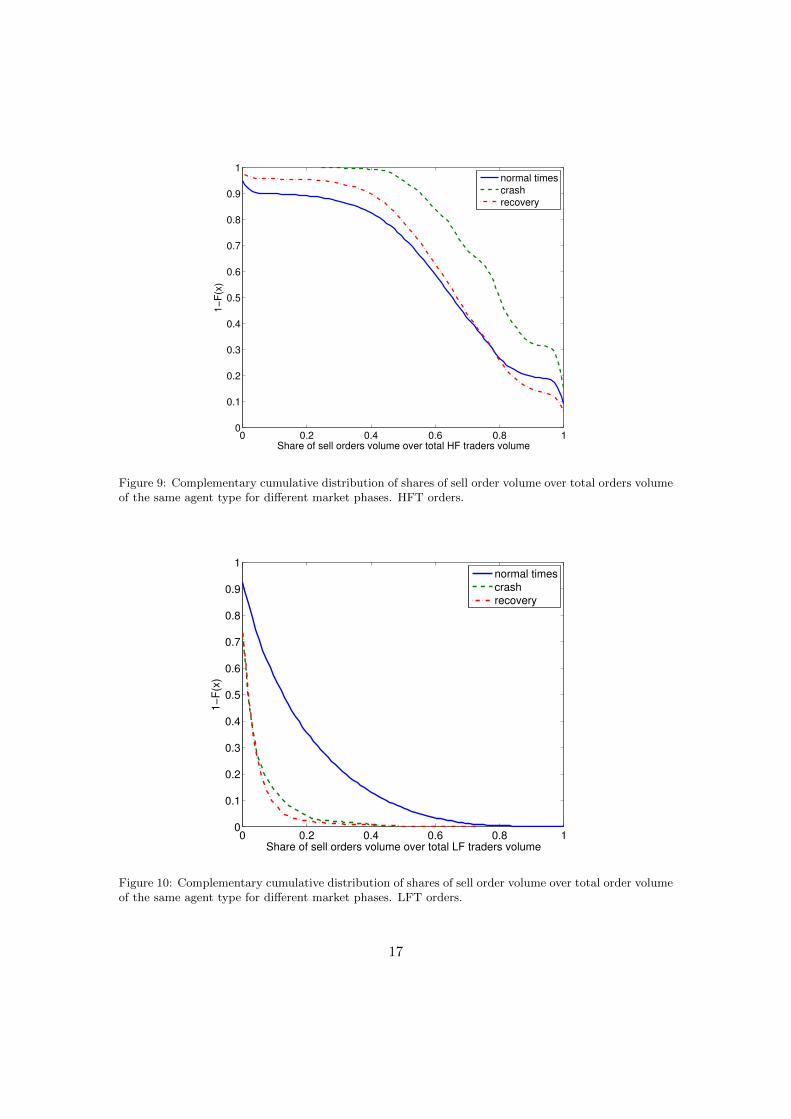
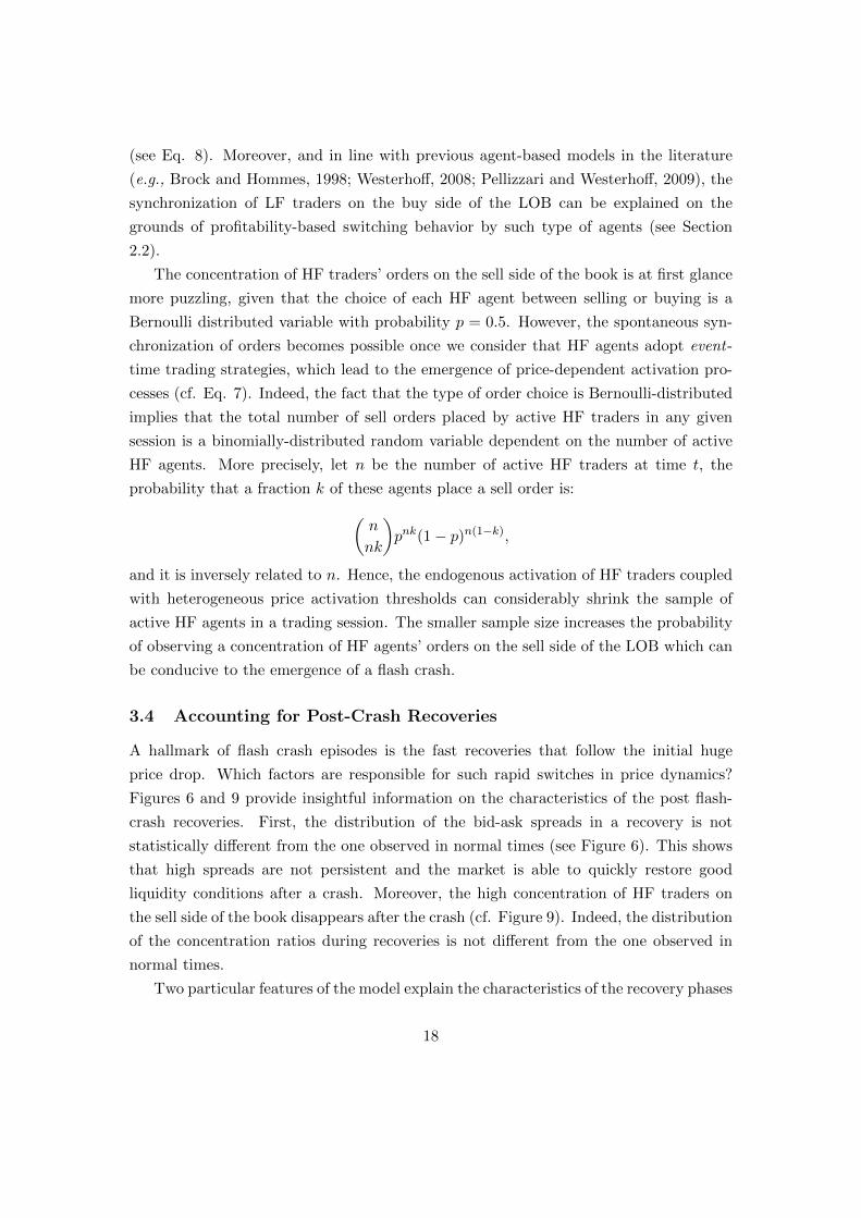
agent and across different market phases (cf. Figures 9 and 10). The complementary
cumulative distributions confirm that flash crashes are generated by the concentration
of HF and LF orders on opposite sides of the LOB. Indeed, during flash crashes, the
distribution of HF orders significantly shifts to the sell side of LOB, whereas the one of
LF orders moves to the left, revealing a strong concentration on buy orders.
The above discussion shows that flash crashes are a true emergent property of the
model generated by the joint occurrence of three distinct events: i) the presence of a
large bid-ask spread; ii) a strong concentration of HF traders’ orders on the sell side of
the LOB; iii) a strong concentration of LF traders’ orders on the buy side of the LOB.
In particular, the first two elements are in line with the empirical evidence about the
market dynamics observed during the flash crash of May 6th, 2010 (CFTC and SEC,
2010; Kirilenko et al, 2011) and confirm the key role played by high-frequency trading in
generating such extreme events in financial markets. Indeed, the emergence of periods
of high market illiquidity is intimately related to the pricing strategies of HF traders
15
−0.2 0 0.2 0.4 0.6 0.8 1 1.20
0.5
1
1.5
2
2.5
3
3.5
4
4.5
5
Share of sell orders volume over total volume per agent type
f(x)
Normal Times
LF traders
HF traders
Figure 7: Kernel densities of shares of sell order volume over total order volume of the same agent type(HFTs: solid line, LFTs: dashed line). Normal times.
−0.2 0 0.2 0.4 0.6 0.8 1 1.20
2
4
6
8
10
12
14
Share of sell orders volume over total volume per agent type
f(x)
Crash
LF traders
HF traders
Figure 8: Kernel densities of shares of sell order volume over total order volume of the same agent type(HFTs: solid line, LFTs: dashed line). Flash Crashes.
16
0 0.2 0.4 0.6 0.8 10
0.1
0.2
0.3
0.4
0.5
0.6
0.7
0.8
0.9
1
Share of sell orders volume over total HF traders volume
1−
F(x
)
normal times
crash
recovery
Figure 9: Complementary cumulative distribution of shares of sell order volume over total orders volumeof the same agent type for different market phases. HFT orders.
0 0.2 0.4 0.6 0.8 10
0.1
0.2
0.3
0.4
0.5
0.6
0.7
0.8
0.9
1
Share of sell orders volume over total LF traders volume
1−
F(x
)
normal times
crash
recovery
Figure 10: Complementary cumulative distribution of shares of sell order volume over total order volumeof the same agent type for different market phases. LFT orders.
17
(see Eq. 8). Moreover, and in line with previous agent-based models in the literature
(e.g., Brock and Hommes, 1998; Westerhoff, 2008; Pellizzari and Westerhoff, 2009), the
synchronization of LF traders on the buy side of the LOB can be explained on the
grounds of profitability-based switching behavior by such type of agents (see Section
2.2).
The concentration of HF traders’ orders on the sell side of the book is at first glance
more puzzling, given that the choice of each HF agent between selling or buying is a
Bernoulli distributed variable with probability p = 0.5. However, the spontaneous syn-
chronization of orders becomes possible once we consider that HF agents adopt event-
time trading strategies, which lead to the emergence of price-dependent activation pro-
cesses (cf. Eq. 7). Indeed, the fact that the type of order choice is Bernoulli-distributed
implies that the total number of sell orders placed by active HF traders in any given
session is a binomially-distributed random variable dependent on the number of active
HF agents. More precisely, let n be the number of active HF traders at time t, the
probability that a fraction k of these agents place a sell order is:(n
nk
)pnk(1 − p)n(1−k),
and it is inversely related to n. Hence, the endogenous activation of HF traders coupled
with heterogeneous price activation thresholds can considerably shrink the sample of
active HF agents in a trading session. The smaller sample size increases the probability
of observing a concentration of HF agents’ orders on the sell side of the LOB which can
be conducive to the emergence of a flash crash.
3.4 Accounting for Post-Crash Recoveries
A hallmark of flash crash episodes is the fast recoveries that follow the initial huge
price drop. Which factors are responsible for such rapid switches in price dynamics?
Figures 6 and 9 provide insightful information on the characteristics of the post flash-
crash recoveries. First, the distribution of the bid-ask spreads in a recovery is not
statistically different from the one observed in normal times (see Figure 6). This shows
that high spreads are not persistent and the market is able to quickly restore good
liquidity conditions after a crash. Moreover, the high concentration of HF traders on
the sell side of the book disappears after the crash (cf. Figure 9). Indeed, the distribution
of the concentration ratios during recoveries is not different from the one observed in
normal times.
Two particular features of the model explain the characteristics of the recovery phases
18
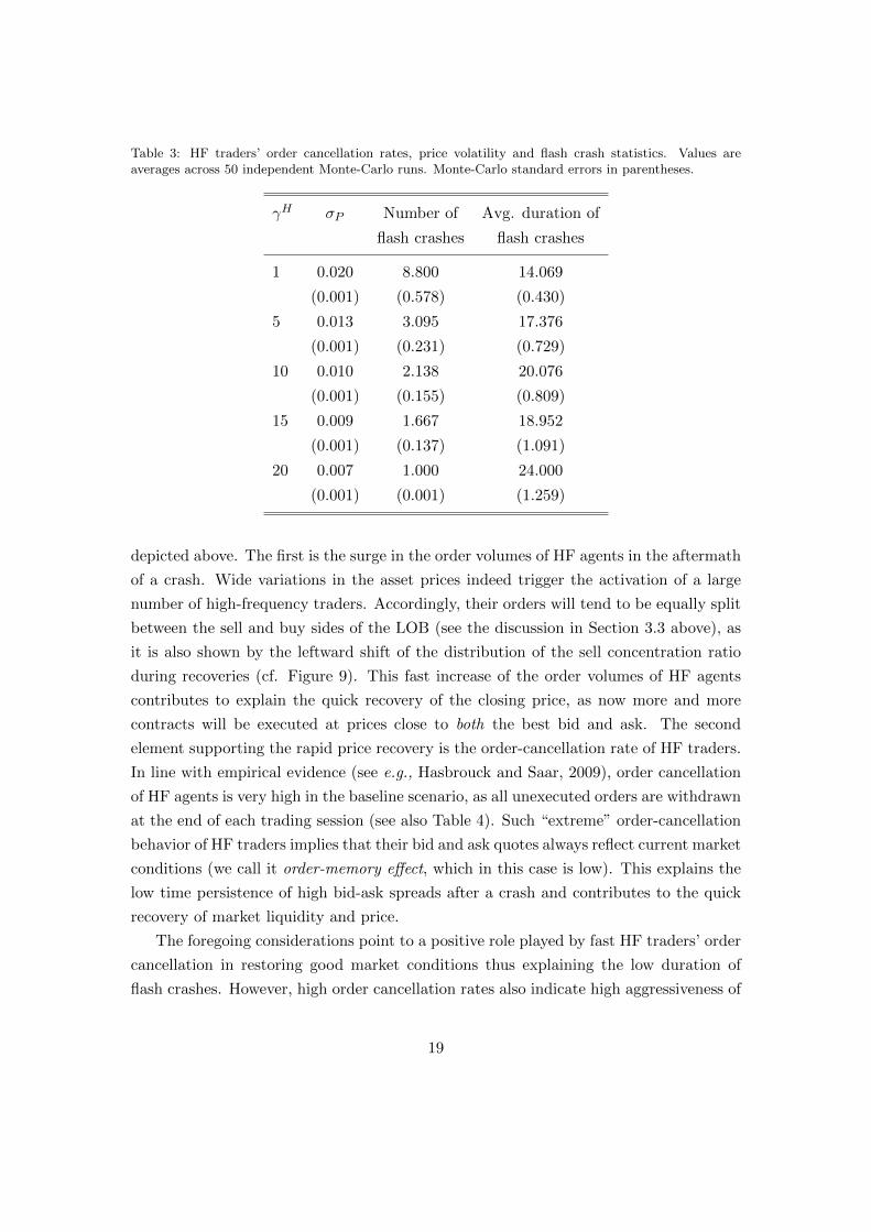
Table 3: HF traders’ order cancellation rates, price volatility and flash crash statistics. Values areaverages across 50 independent Monte-Carlo runs. Monte-Carlo standard errors in parentheses.
γH σP Number of Avg. duration of
flash crashes flash crashes
1 0.020 8.800 14.069
(0.001) (0.578) (0.430)
5 0.013 3.095 17.376
(0.001) (0.231) (0.729)
10 0.010 2.138 20.076
(0.001) (0.155) (0.809)
15 0.009 1.667 18.952
(0.001) (0.137) (1.091)
20 0.007 1.000 24.000
(0.001) (0.001) (1.259)
depicted above. The first is the surge in the order volumes of HF agents in the aftermath
of a crash. Wide variations in the asset prices indeed trigger the activation of a large
number of high-frequency traders. Accordingly, their orders will tend to be equally split
between the sell and buy sides of the LOB (see the discussion in Section 3.3 above), as
it is also shown by the leftward shift of the distribution of the sell concentration ratio
during recoveries (cf. Figure 9). This fast increase of the order volumes of HF agents
contributes to explain the quick recovery of the closing price, as now more and more
contracts will be executed at prices close to both the best bid and ask. The second
element supporting the rapid price recovery is the order-cancellation rate of HF traders.
In line with empirical evidence (see e.g., Hasbrouck and Saar, 2009), order cancellation
of HF agents is very high in the baseline scenario, as all unexecuted orders are withdrawn
at the end of each trading session (see also Table 4). Such “extreme” order-cancellation
behavior of HF traders implies that their bid and ask quotes always reflect current market
conditions (we call it order-memory effect, which in this case is low). This explains the
low time persistence of high bid-ask spreads after a crash and contributes to the quick
recovery of market liquidity and price.
The foregoing considerations point to a positive role played by fast HF traders’ order
cancellation in restoring good market conditions thus explaining the low duration of
flash crashes. However, high order cancellation rates also indicate high aggressiveness of
19
HF traders in exploiting the orders placed by LF agents in the LOB (we call it liquidity-
fishing effect). This favors the emergence of high bid-ask spreads in the market thus
increasing the probability of observing a large fall in the asset price.
To further explore the role of HF traders’ order cancellation on price fluctuations, we
perform a Monte-Carlo experiment where we vary the number of periods an unexecuted
HFT order stays in the book (measured by the parameter γH), while keeping all the
other parameters at their baseline values. The results of this experiment are reported in
Table 3. We find that a reduction in the order cancellation rate (higher γH , see Table
3) decreases market volatility and the number of flash-crash episodes.14 This outcome
stems from the lower aggressiveness of HF traders’ strategies as order cancellation rates
decrease, i.e. the liquidity-fishing effect becomes weaker. In contrast, the duration of
flash crashes is inversely related to the order cancellation rate (cf. fourth column of
Table 3). This outcome can be explained by the order-memory effect. As γH increases,
the bid and ask quotes posted by HF agents stay longer in the LOB thus raising the
number of contracts traded at prices close to the crash one. In turn, this hinders the
recovery of the market price.
4 Concluding Remarks
We developed an agent-based model of a limit-order book (LOB) market to study how
the interplay between low- and high-frequency traders shapes asset price dynamics and
eventually leads to flash crashes. In the model, low-frequency traders can switch between
fundamentalist and chartist strategies. High-frequency (HF) traders employ directional
strategies to exploit the order book information released by low-frequency (LF) agents.
In addition, LF trading rules are based on chronological time, whereas HF ones are
framed in event time, i.e. the activation of HF traders endogenously depends on past
price fluctuations.
We showed that the model is able to replicate the main stylized facts of financial
markets. Moreover, the presence of HF traders generates periods of high market volatil-
ity and sharp price drops with statistical properties akin to the ones observed in the
empirical literature. In particular, the emergence of flash crashes is explained by the
interplay of three factors: i) HF traders causing periods of high illiquidity represented
by large bid-ask spreads; ii) the synchronization of HF traders’ orders on the sell-side of
the LOB; iii) the concentration of LF traders on the buy side of the book.
14We also carried out simulations for γH > 20. The above patterns are confirmed. Interestingly, flashcrashes completely disappear when the order cancellation rate is very low.
20
Finally, we have investigated the recovery phases that follow price-crash events, find-
ing that HF traders’ order cancellations play a key role in shaping asset price volatility
and the frequency as well as the duration of flash crashes. Indeed, higher order can-
cellation rates imply higher market volatility and a higher occurrence of flash crashes.
However, we establish that they speed up the recovery of market price after a crash.
Our results suggest that order cancellation strategies of HF traders cast more complex
effects than thought so far, and that regulatory policies aimed at curbing such practices
(e.g., the imposition of cancellation fees, see also Ait-Sahalia and Saglam, 2013) should
take such effects into account.
Our model could be extended in at least three ways. First, we have made several
departures from the zero-intelligence framework, which has been so far the standard
in agent-based models of HFT. However, one can play with agents’ strategic repertoires
even further. For example, one could allow HF traders to switch between sets of different
strategies with increasing degrees of sophistication. Second, we have considered only one
asset market in the model. However, taking into account more than one market would
allow one to consider other relevant aspects of HFT and flash crashes such as the possible
emergence of systemic crashes triggered by sudden and huge price drops in one market
(see CFTC and SEC, 2010). In addition, another salient feature of HF traders is the
ability to rapidly process and profit from the information coming from different markets
i.e., latency arbitrage strategies (e.g., Wah and Wellman, 2013). Third, and finally,
one could employ the model as a test-bed for a number of policy interventions directed
to affect high-frequency trading and therefore mitigating the effects of flash crashes.
Besides the aforementioned example of order cancellation fees, the possible policy list
could include measures such as the provision of different types of trading halt facilities
and the introduction of a tax on high-frequency transactions.
Acknowledgments
We are grateful to Sylvain Barde, Francesca Chiaromonte, Antoine Godin, Alan Kirman, Nobi Hanaki,Fabrizio Lillo, Frank Westerhoff, for stimulating comments and fruitful discussions. We also thank theparticipants of the Workshop on Heterogeneity and Networks in (Financial) Markets in Marseille, March2013, of the EMAEE conference in Sophia Antipolis, May 2013, of the WEHIA conference in Reykiavik,June 2013, of the 2013 CEF conference in Vancouver, July 2013 and of the SFC workshop in Limerick,August 2013 where earlier versions of this paper were presented. All usual disclaimers apply. The authorsgratefully acknowledge the financial support of the Institute for New Economic Thinking (INET) grants#220, “The Evolutionary Paths Toward the Financial Abyss and the Endogenous Spread of FinancialShocks into the Real Economy”.
21
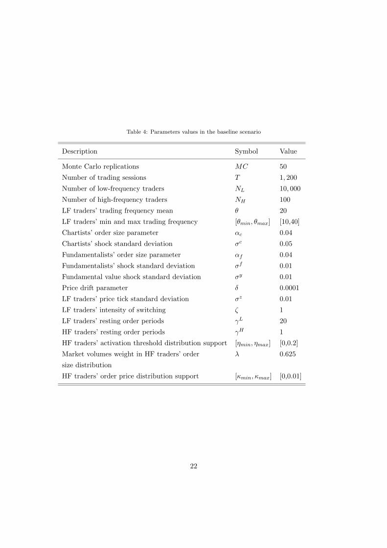
Table 4: Parameters values in the baseline scenario
Description Symbol Value
Monte Carlo replications MC 50
Number of trading sessions T 1, 200
Number of low-frequency traders NL 10, 000
Number of high-frequency traders NH 100
LF traders’ trading frequency mean θ 20
LF traders’ min and max trading frequency [θmin, θmax] [10,40]
Chartists’ order size parameter αc 0.04
Chartists’ shock standard deviation σc 0.05
Fundamentalists’ order size parameter αf 0.04
Fundamentalists’ shock standard deviation σf 0.01
Fundamental value shock standard deviation σy 0.01
Price drift parameter δ 0.0001
LF traders’ price tick standard deviation σz 0.01
LF traders’ intensity of switching ζ 1
LF traders’ resting order periods γL 20
HF traders’ resting order periods γH 1
HF traders’ activation threshold distribution support [ηmin, ηmax] [0,0.2]
Market volumes weight in HF traders’ order λ 0.625
size distribution
HF traders’ order price distribution support [κmin, κmax] [0,0.01]
22
References
Ait-Sahalia Y, Saglam M (2013) High frequency traders: Taking advantage of speed. NBER WorkingPapers 19531, National Bureau of Economic Research
Aloud M, Tsang E, Olsen R, Dupuis A (2011) A directional-change events approach for studying financialtime series. Economics Discussion Paper (2011-28)
Aloud M, Tsang E, Olsen R (2013) Modeling the fx market traders’ behavior: An agent-based approach.In: Alexandrova-Kabadjova B, Martinez-Jaramillo S, Garcia-Almanza A, Tsang E (eds) Simulationin Computational Finance and Economics: Tools and Emerging Applications, Hershey, PA: BusinessScience Reference
Ane T, Geman H (2000) Order flow, transaction clock and normality of asset returns. Journal of Finance55:2259–2284
Avellaneda M, Stoikov S (2008) High-frequency trading in a limit order book. Quantitative Finance8(3):217–224
Bartolozzi M (2010) A multi agent model for the limit order book dynamics. European Physical JournalB: Condensed Matter Physics 78(2):265–273
Bouchaud JP, Mezard M, Potters M, et al (2002) Statistical properties of stock order books: empiricalresults and models. Quantitative Finance 2(4):251–256
Brock W, Hommes C (1998) Heterogeneous beliefs and routes to chaos in a simple asset pricing model.Journal of Economic Dynamics and Control 22(8-9):1235–1274
Brogaard J (2010) High frequency trading and its impact on market quality. Northwestern UniversityKellogg School of Management Working Paper
Brundsen J (2012) Traders may face nordic-style eu fees for canceled orders. Bloomberg News, march23rd, 2012
CFTC, SEC (2010) Findings regarding the market events of may 6, 2010. Report of the Staffs of theCFTC and SEC to the Joint Advisory Committee on Emerging Regulatory Issues
Chakraborti A, Toke IM, Patriarca M, Abergel F (2011) Econophysics review: I. empirical facts. Quan-titative Finance 11(7):991–1012
Chiarella C (1992) The dynamics of speculative behaviour. Annals Of Operations Research 37(1):101–123
Chiarella C, He X (2003) Heterogeneous beliefs, risk, and learning in a simple asset-pricing model witha market maker. Macroeconomic Dynamics 7(4):503–536
Chiarella C, He X, Hommes C (2006) A dynamic analysis of moving average rules. Journal of EconomicDynamics and Control 30(9):1729–1753
Clark PK (1973) A subordinated stochastic process model with finite variance for speculative prices.Econometrica 41:135–155
Cont R (2001) Empirical properties of asset returns: stylized facts and statistical issues. QuantitativeFinance 1(2):223–236
Cont R, Potters M, Bouchaud JP (1997) Scaling in stock market data: stable laws and beyond. Paperscond-mat/9705087, arXiv.org
23
Cvitanic J, Kirilenko A (2010) High frequency traders and asset prices. Available at SSRN 1569075
Easley D, Lopez de Prado M, O’Hara M (2012) The volume clock: Insights into the high frequencyparadigm. Journal of Portfolio Management 39(1):19–29
Economist T (2012) The fast and the furious. The Economist, february 25th, 2012
Fama E (1970) Efficient capital markets: A review of theory and empirical work. Journal of Finance25(2):383–417
Farmer JD (2002) Market force, ecology and evolution. Industrial and Corporate Change 11(5):895–953
Farmer JD, Gillemot L, Lillo F, Szabolcs M, Sen A (2004) What really causes large price changes?Quantitative Finance 4(4):383–397
Farmer JD, Patelli P, Zovko II (2005) The predictive power of zero intelligence in financial markets.PNAS 102(6)
Hanson TA (2011) The effects of high frequency traders in a simulated market. Available at SSRN1918570
Hasbrouck J, Saar G (2009) Technology and liquidity provision: The blurring of traditional definitions.J Finan Mark 12(2):143–172
Hommes C, Huang H, Wang D (2005) A robust rational route to randomness in a simple asset pricingmodel. Journal of Economic Dynamics and Control 29(6):1043–1072
Kirilenko A, Kyle A, Samadi M, Tuzun T (2011) The flash crash: The impact of high frequency tradingon an electronic market. Available at SSRN 1686004
Lo AW, MacKinlay AC (1999) A Non-Random Walk Down Wall Street. Princeton University Press
Luckock H (2003) A steady-state model of the continuous double auction. Quantitative Finance 3(5):385–404
Lux T (1995) Herd behaviour, bubbles and crashes. Economic Journal 105(431):881–896
Lux T (2006) Financial power laws: Empirical evidence, models, and mechanism. Economics WorkingPapers 2006,12, Christian-Albrechts-University of Kiel, Department of Economics
Lux T, Marchesi M (2000) Volatility clustering in financial markets: A microsimulation of interactingagents. International Journal of Theoretical and Applied Finance 3(4):675–702
Mandelbrot B (1963) The variation of certain speculative prices. Journal of Business 36(4):394–419
Mandelbrot B, Taylor M (1967) On the distribution of stock price differences. Operations Research15:1057–162
Maslov S (2000) Simple model of a limit order-driven market. Physica A: Statistical Mechanics and itsApplications 278(3):571–578
Menkveld AJ (2013) High frequency trading and the new-market makers. Quarterly Journal of Economics128(1):249–85
Paddrik ME, Hayes RL, Todd A, Yang SY, Scherer W, Beling P (2011) An agent based model of thee-mini s&p 500 and the flash crash. Available at SSRN 1932152
Pagan A (1996) The econometrics of financial markets. Journal of Empirical Finance 3(1):15–102
24
Patterson S, Ackerman A (2012) Sec may ticket speeding traders. Wall Street Journal, february 23rd,2012
Pellizzari P, Westerhoff F (2009) Some effects of transaction taxes under different microstructures. Jour-nal of Economic Behavior and Organization 72(3):850–863
SEC (2010) Concept release on equity market structure. Release No. 34-61358, january 14, 2010. Avail-able at: http://www.sec.gov/rules/concept/2010/34-61358.pdf
Slanina F (2008) Critical comparison of several order-book models for stock-market fluctuations. Euro-pean Physical Journal B: Condensed Matter Physics 61(2):225–240
Smith E, Farmer JD, Gillemot Ls, Krishnamurthy S (2003) Statistical theory of the continuous doubleauction. Quantitative Finance 3(6):481–514
Sornette D, Von der Becke S (2011) Crashes and high frequency trading. Swiss Finance Institute ResearchPaper (11-63)
Wah E, Wellman MP (2013) Latency arbitrage, market fragmentation, and efficiency: a two-marketmodel. In: Proceedings of the fourteenth ACM conference on Electronic commerce, ACM, pp 855–872
Westerhoff FH (2008) The use of agent-based financial market models to test the effectiveness of regu-latory policies. Jahr Nationaloekon Statist 228(2):195
Zhang F (2010) High-frequency trading, stock volatility, and price discovery. Available at SSRN 1691679
Zovko I, Farmer JD (2002) The power of patience: a behavioural regularity in limit-order placement.Quantitative Finance 2(5):387–392
25