1

PHOTOCHEMISTRY

Prof. M.N.R. Ashfold (S305)

Fates of Excited State Molecules • absorption and emission of electromagnetic radiation • Einstein coefficients, absorption probabilities • fluorescence and phosphorescence • internal conversion and intersystem crossing • photodissociation and predissociation • Jablonski diagram Lasers • requirements for laser action • population inversions • properties of laser radiation • examples of lasers • applications in spectroscopy and photochemistry Photodissociation and Predissociation • viewed from perspective of (a) the excited parent molecule, and (b) the resulting photofragments • Ozone photochemistry, the stratospheric ozone 'deficit' and ozone photochemistry in the troposphere Femtochemistry • following photochemically induced processes in real time

2

Absorption and emission of electromagnetic (EM) radiation

by atoms and molecules Photochemical processes (e.g. photodissociations) are initiated by the absorption of EM radiation (i.e. light).

This absorption is induced by the electric (rE) field of

the EM radiation [in the case of an electric dipole (or electric quadrupole) interaction], or the magnetic (

rB)

field [magnetic dipole interaction]. Electric dipole transitions are typically ~105 times stronger than those carried by a magnetic dipole interaction, and ~107 times more intense than electric quadrupole transitions. Thus we shall concentrate on electric dipole transitions. In the presence of EM radiation a molecule experiences a perturbation described by the dipolar interaction:

$h(t) = − $µ .rE(t) (1.1)

where the time-dependence recognises the oscillatory nature of the EM field. $µ is the transition dipole moment operator (not the permanent dipole moment), and rE(t) =

rE 0cosωt, where

rE 0 is the amplitude of the

rE field

and ω is the (angular) frequency ≡ 2πν.

3

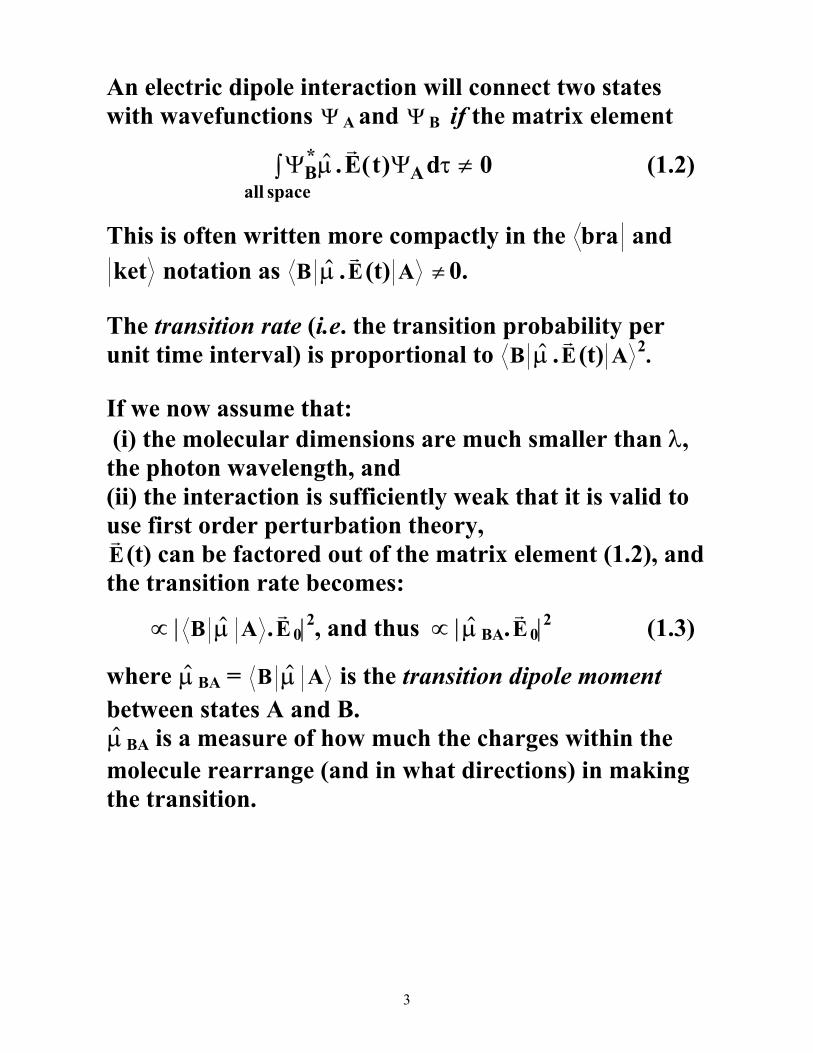
An electric dipole interaction will connect two states with wavefunctions Ψ A and Ψ B if the matrix element

Ψ ΨB Aall space

E t d* $ . ( )µ τr

∫ ≠ 0 (1.2)

This is often written more compactly in the bra and ket notation as B $µ .

rE(t) A ≠ 0.

The transition rate (i.e. the transition probability per unit time interval) is proportional to B $µ .

rE(t) A 2.

If we now assume that: (i) the molecular dimensions are much smaller than λ, the photon wavelength, and (ii) the interaction is sufficiently weak that it is valid to use first order perturbation theory, rE(t) can be factored out of the matrix element (1.2), and the transition rate becomes:

∝ | B $µ A .rE 0|2, and thus ∝ | $µ BA.

rE 0|2 (1.3)

where $µ BA = B $µ A is the transition dipole moment between states A and B. $µ BA is a measure of how much the charges within the molecule rearrange (and in what directions) in making the transition.

4

Absorption is one of three possible processes by which resonant radiation can induce transfer of population between two states A and B.

Rate = BAB [A] ρ(νAB) (1.4) BAB = Einstein coefficient for (stimulated) absorption:

BAB = 1

6 02ε h

| B $µ A |2 (1.5)

[A] = number density in state A ρ(νAB) = spectral energy density (a measure of light intensity, with units: J m-3 s).

5

The other two processes involve emission, i.e.

Spontaneous emission

Rate = ABA [B] (1.6) ABA = Einstein coefficient for spontaneous emission

ABA = 8 3

3π νhc

BBA (1.7)

The ν3 factor in the numerator means that, other things being equal, excited states at higher energies will have a faster radiative decay rate.

Stimulated emission

Rate = BBA [B] ρ(νBA) (1.8) BBA = Einstein coefficient for stimulated emission

= gg

BA

BAB , (1.9)

where gA is the degeneracy of state A, etc. The stimulated photon has the same frequency and direction as the stimulating photon.

6

Question. What determines the strength of a spectral transition?

Answer. The transition probability is determined by B $µ A 2. In molecules, this 'electronic' transition strength is sub-divided by vibrational and rotational fine-structure, governed by Franck-Condon factors and rotational linestrengths, respectively.

Symmetry considerations can tell us if $µ BA = 0. (recall NCN and CMW Level 3 lectures), e.g.

For atoms: ∆l = ±1 (the Laporte selection rule).

The spin quantum number, S, should be conserved, i.e. ∆S = 0, though this becomes less restrictive if the spin-orbit coupling is large (e.g. in heavier atoms, or in molecules containing at least one heavy atom).

For linear molecules (where states are classified by a quantum number Λ, which defines the axial projection of the orbital angular momentum, e.g. Σ, Π, ∆, etc.): ∆Λ = 0, or ±1.

If spin-orbit coupling is important, Λ is no longer a good quantum number, but the axial projection of the total electronic angular momentum (Ω, the sum of Λ and S) is: ∆Ω = 0, or ±1.

For centrosymmetric molecules, g↔ u.

These are often called electric dipole selection rules.

7

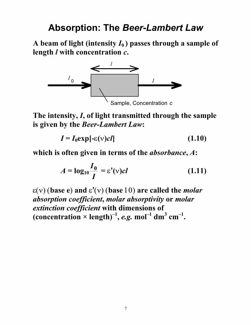
Absorption: The Beer-Lambert Law

A beam of light (intensity I0 ) passes through a sample of length l with concentration c.

I 0 I

l

Sample, Concentration c

The intensity, I, of light transmitted through the sample is given by the Beer-Lambert Law:

I = I0exp[-ε(ν)cl] (1.10)

which is often given in terms of the absorbance, A:

A = log10II0 = ε’(ν)cl (1.11)

ε(ν) (base e) and ε’(ν) (base 10) are called the molar absorption coefficient, molar absorptivity or molar extinction coefficient with dimensions of (concentration × length)–1, e.g. mol–1 dm3 cm–1.

8

Absorption profiles often span a spread of frequencies. It is thus usual to quote the maximum absorption, εmax.

ε(ν) is related to the Einstein coefficient (and thus the transition dipole moment) by:

( )BLh

dABAB

= ∫ln10

1

2

νε ν νν

ν . (1.12)

L is the Avogadro number and ν AB is the average frequency of the transition.

9

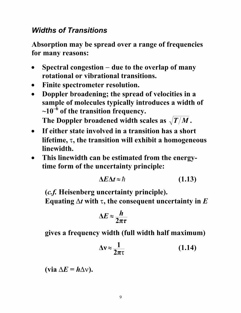
Widths of Transitions

Absorption may be spread over a range of frequencies for many reasons:

• Spectral congestion − due to the overlap of many rotational or vibrational transitions.

• Finite spectrometer resolution. • Doppler broadening; the spread of velocities in a

sample of molecules typically introduces a width of ~10–6 of the transition frequency. The Doppler broadened width scales as T M .

• If either state involved in a transition has a short lifetime, τ, the transition will exhibit a homogeneous linewidth.

• This linewidth can be estimated from the energy-time form of the uncertainty principle:

h≈tE∆∆ (1.13)

(c.f. Heisenberg uncertainty principle). Equating ∆t with τ, the consequent uncertainty in E

τhE 2π∆ ≈

gives a frequency width (full width half maximum)

τ2π1∆ν≈ (1.14)

(via ∆E = h∆ν).

10

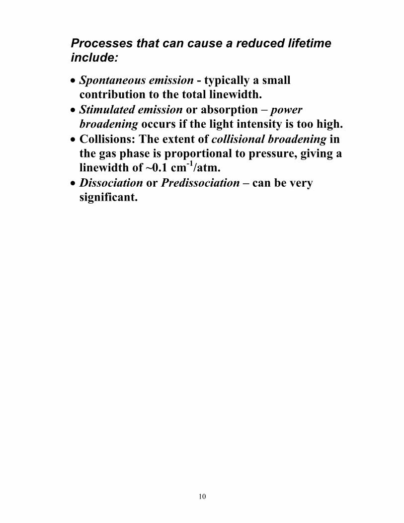
Processes that can cause a reduced lifetime include:

• Spontaneous emission - typically a small contribution to the total linewidth.

• Stimulated emission or absorption − power broadening occurs if the light intensity is too high.

• Collisions: The extent of collisional broadening in the gas phase is proportional to pressure, giving a linewidth of ~0.1 cm-1/atm.

• Dissociation or Predissociation – can be very significant.

11

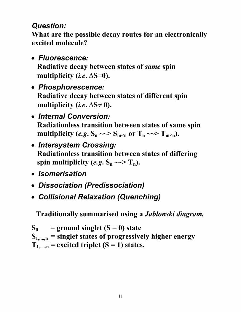
Question: What are the possible decay routes for an electronically excited molecule?

• Fluorescence: Radiative decay between states of same spin multiplicity (i.e. ∆S=0).

• Phosphorescence: Radiative decay between states of different spin multiplicity (i.e. ∆S≠ 0).

• Internal Conversion: Radiationless transition between states of same spin multiplicity (e.g. Sn ~~> Sm<n or Tn ~~> Tm<n).

• Intersystem Crossing: Radiationless transition between states of differing spin multiplicity (e.g. Sn ~~> Tn).

• Isomerisation

• Dissociation (Predissociation)

• Collisional Relaxation (Quenching)

Traditionally summarised using a Jablonski diagram.

S0 = ground singlet (S = 0) state S1,....,n = singlet states of progressively higher energy T1,....,n = excited triplet (S = 1) states.

12

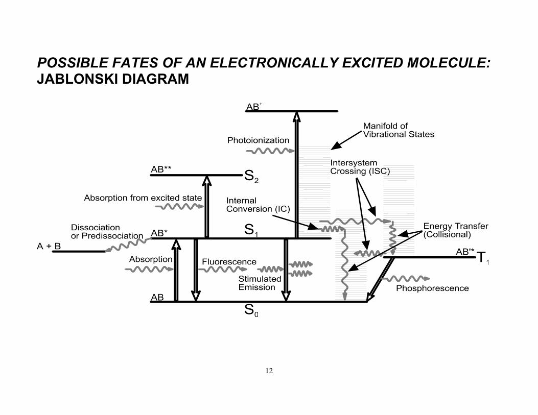
POSSIBLE FATES OF AN ELECTRONICALLY EXCITED MOLECULE: JABLONSKI DIAGRAM

13

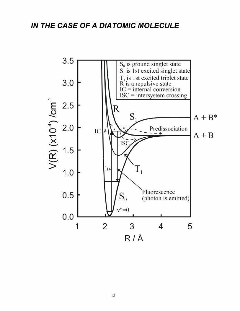
IN THE CASE OF A DIATOMIC MOLECULE

14

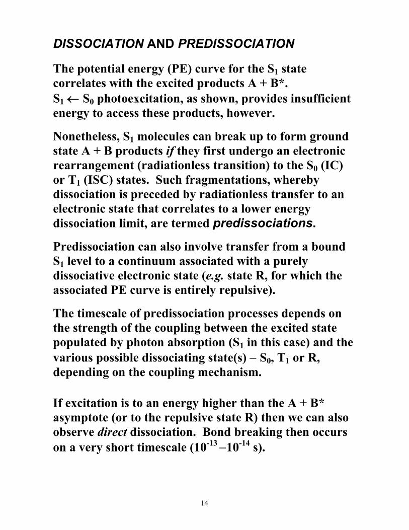
DISSOCIATION AND PREDISSOCIATION The potential energy (PE) curve for the S1 state correlates with the excited products A + B*. S1 ← S0 photoexcitation, as shown, provides insufficient energy to access these products, however.

Nonetheless, S1 molecules can break up to form ground state A + B products if they first undergo an electronic rearrangement (radiationless transition) to the S0 (IC) or T1 (ISC) states. Such fragmentations, whereby dissociation is preceded by radiationless transfer to an electronic state that correlates to a lower energy dissociation limit, are termed predissociations.

Predissociation can also involve transfer from a bound S1 level to a continuum associated with a purely dissociative electronic state (e.g. state R, for which the associated PE curve is entirely repulsive).

The timescale of predissociation processes depends on the strength of the coupling between the excited state populated by photon absorption (S1 in this case) and the various possible dissociating state(s) − S0, T1 or R, depending on the coupling mechanism.

If excitation is to an energy higher than the A + B* asymptote (or to the repulsive state R) then we can also observe direct dissociation. Bond breaking then occurs on a very short timescale (10-13 −10-14 s).

15

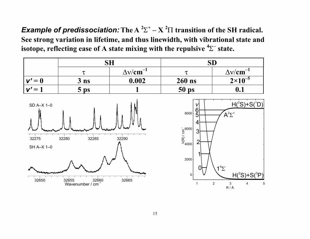
Example of predissociation: The A 2Σ+ – X 2Π transition of the SH radical. See strong variation in lifetime, and thus linewidth, with vibrational state and isotope, reflecting ease of A state mixing with the repulsive 4Σ– state.

SH SD τ ∆ν/cm–1 τ ∆ν/cm–1

v' = 0 3 ns 0.002 260 ns 2×10–5 v' = 1 5 ps 1 50 ps 0.1

16

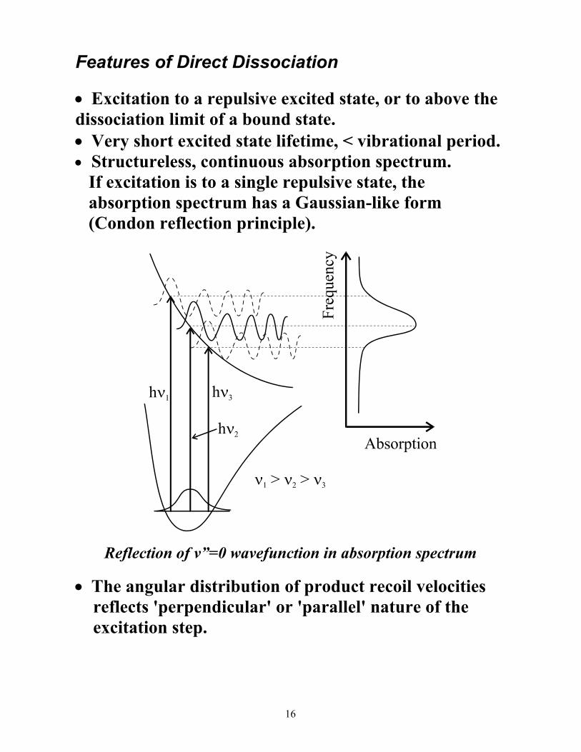
Features of Direct Dissociation

• Excitation to a repulsive excited state, or to above the dissociation limit of a bound state. • Very short excited state lifetime, < vibrational period. • Structureless, continuous absorption spectrum. If excitation is to a single repulsive state, the absorption spectrum has a Gaussian-like form (Condon reflection principle).

Reflection of v”=0 wavefunction in absorption spectrum

• The angular distribution of product recoil velocities reflects 'perpendicular' or 'parallel' nature of the excitation step.

17

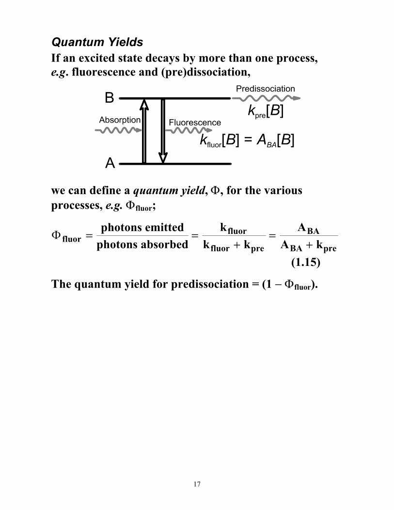
Quantum Yields

If an excited state decays by more than one process, e.g. fluorescence and (pre)dissociation,

we can define a quantum yield, Φ, for the various processes, e.g. Φfluor;

ΦfluorBA

BA

kk k

AA k

= =+

=+

photons emittedphotons absorbed

fluor

fluor pre pre

(1.15)

The quantum yield for predissociation = (1 − Φfluor).

18

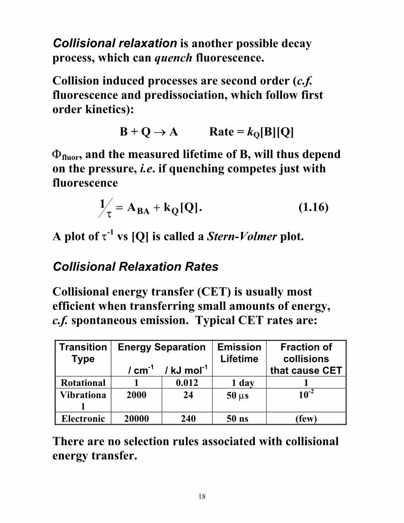
Collisional relaxation is another possible decay process, which can quench fluorescence.

Collision induced processes are second order (c.f. fluorescence and predissociation, which follow first order kinetics):

B + Q → A Rate = kQ[B][Q]

Φfluor, and the measured lifetime of B, will thus depend on the pressure, i.e. if quenching competes just with fluorescence

1τ = +A kBA Q Q[ ]. (1.16)

A plot of τ-1 vs [Q] is called a Stern-Volmer plot.

Collisional Relaxation Rates

Collisional energy transfer (CET) is usually most efficient when transferring small amounts of energy, c.f. spontaneous emission. Typical CET rates are:

Transition Type

Energy Separation / cm-1 / kJ mol-1

Emission Lifetime

Fraction of collisions

that cause CETRotational 1 0.012 1 day 1 Vibrationa

l 2000 24 50 µs 10-2

Electronic 20000 240 50 ns (few)

There are no selection rules associated with collisional energy transfer.

19

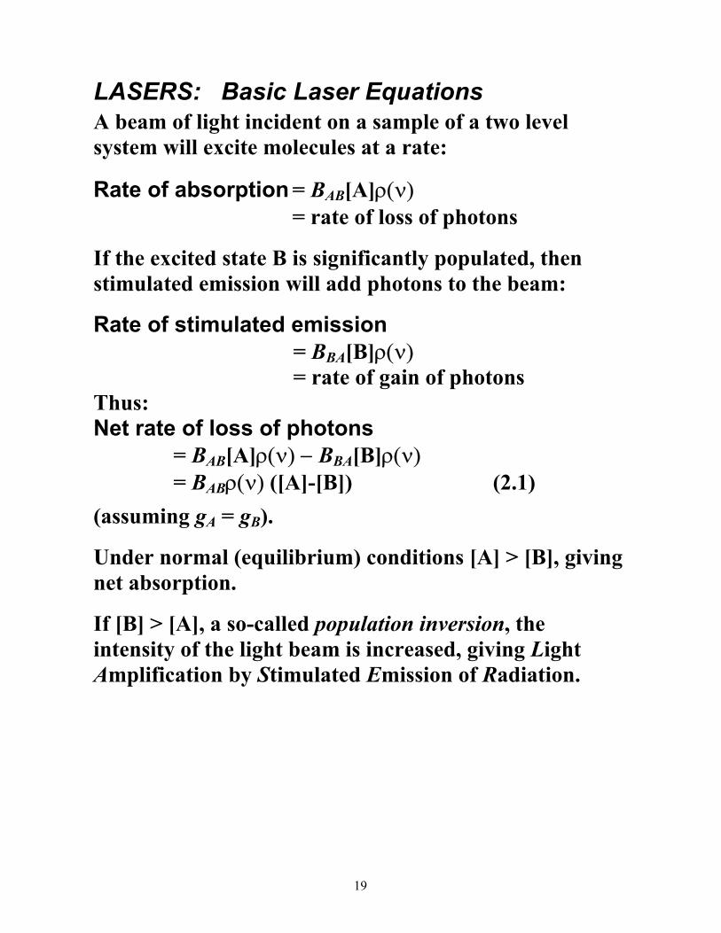
LASERS: Basic Laser Equations A beam of light incident on a sample of a two level system will excite molecules at a rate:

Rate of absorption = BAB[A]ρ(ν) = rate of loss of photons

If the excited state B is significantly populated, then stimulated emission will add photons to the beam:

Rate of stimulated emission = BBA[B]ρ(ν) = rate of gain of photons

Thus: Net rate of loss of photons

= BAB[A]ρ(ν) − BBA[B]ρ(ν) = BABρ(ν) ([A]-[B]) (2.1)

(assuming gA = gB).

Under normal (equilibrium) conditions [A] > [B], giving net absorption.

If [B] > [A], a so-called population inversion, the intensity of the light beam is increased, giving Light Amplification by Stimulated Emission of Radiation.

20

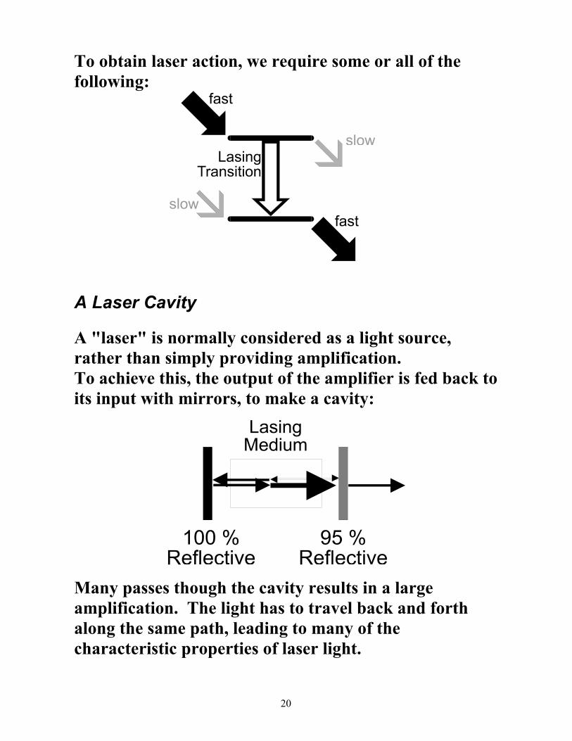
To obtain laser action, we require some or all of the following:

A Laser Cavity

A "laser" is normally considered as a light source, rather than simply providing amplification. To achieve this, the output of the amplifier is fed back to its input with mirrors, to make a cavity:

Many passes though the cavity results in a large amplification. The light has to travel back and forth along the same path, leading to many of the characteristic properties of laser light.

21

Properties of Laser Light

1. Low divergence. The light from a laser is very parallel. Thus:

• laser radiation will travel long distances without spreading – useful in LIDAR (see below).

• it can be focused to a very small spot, of the order of the wavelength of the light. This implies small sample volumes, and high power densities.

2. Coherent, implying a fixed phase relationship between different parts of the laser beam. This ensures that applications which rely on interference, like holography, will work effectively.

3. Monochromatic. The best lasers have a frequency spread of 1 part in 109, implying very accurate measurement and resolution of very small splittings.

4. Very short pulses − the shortest pulses are of the order of 10 fs (= 10–14 s), comparable to the time scale of atoms moving during a reaction (such pulses necessarily span a wide range of frequencies).

5. High intensities. Tight focusing and a narrow frequency spread mean that transitions can be excited very efficiently. Pulsed lasers can provide GW (109 W, the output of several power stations) powers for short periods. Thus very weak transitions, including multiphoton transitions, can be excited. These have different selection rules (like Raman, only applied to electronic transitions).

22

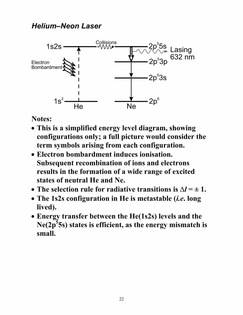
Helium–Neon Laser

Notes: • This is a simplified energy level diagram, showing

configurations only; a full picture would consider the term symbols arising from each configuration.

• Electron bombardment induces ionisation. Subsequent recombination of ions and electrons results in the formation of a wide range of excited states of neutral He and Ne.

• The selection rule for radiative transitions is ∆l = ± 1. • The 1s2s configuration in He is metastable (i.e. long

lived). • Energy transfer between the He(1s2s) levels and the

Ne(2p55s) states is efficient, as the energy mismatch is small.

23

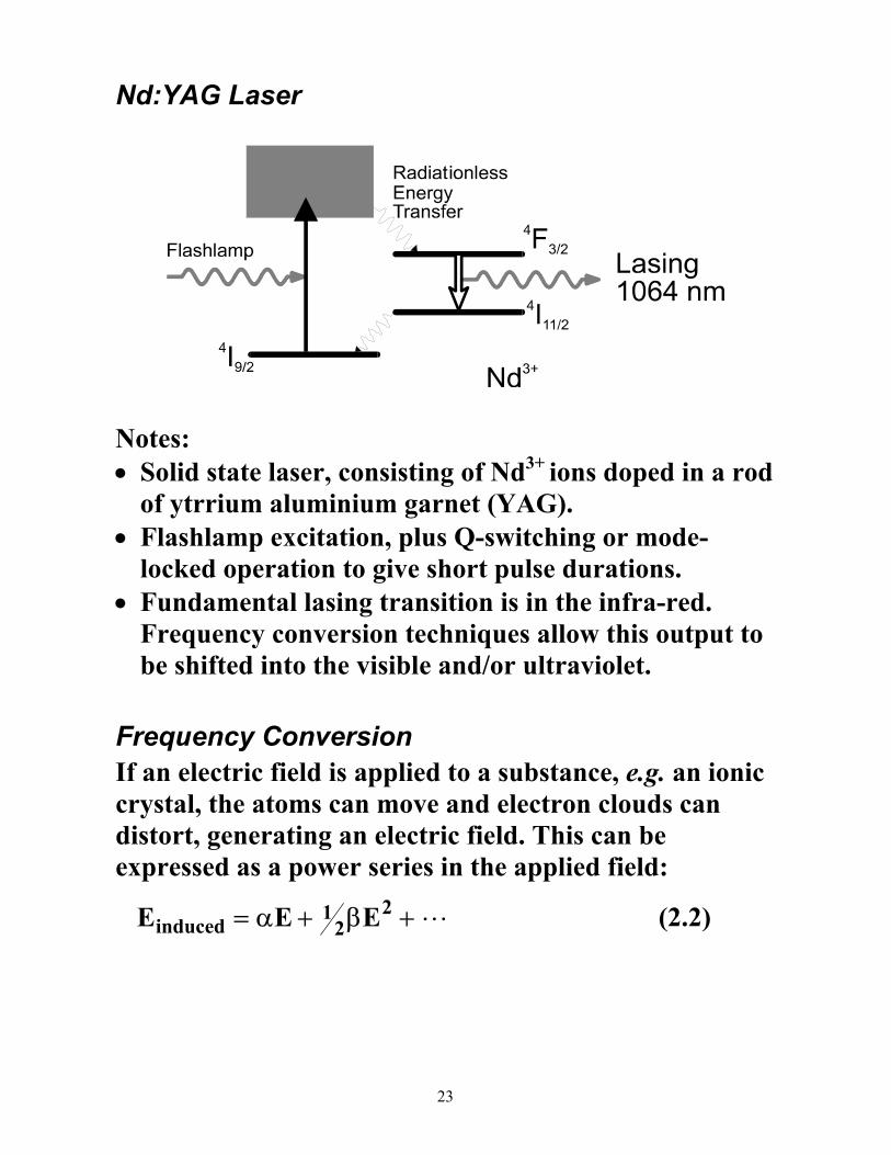
Nd:YAG Laser

Notes: • Solid state laser, consisting of Nd3+ ions doped in a rod

of ytrrium aluminium garnet (YAG). • Flashlamp excitation, plus Q-switching or mode-

locked operation to give short pulse durations. • Fundamental lasing transition is in the infra-red.

Frequency conversion techniques allow this output to be shifted into the visible and/or ultraviolet.

Frequency Conversion If an electric field is applied to a substance, e.g. an ionic crystal, the atoms can move and electron clouds can distort, generating an electric field. This can be expressed as a power series in the applied field:

E E Einduced = + +α β12

2 L (2.2)

24

where E is the applied field. If we take this to vary as E0cos ωt then the induced field will contain a component at twice this input frequency, i.e.

( )E E t E tinduced = = +12 0

2 2 14 0

2 1 2β ω β ωcos cos (2.3)

This is second harmonic generation or frequency doubling. The efficiency depends critically on the material used and requires high light intensities.

Commonly used non-linear materials include KDP (KH2PO4) and BBO (β-BaB2O4), both of which are used to 'double' the frequency of the output of dye lasers and Nd:YAG lasers (e.g. 1064 nm → 532 nm).

Frequency sum and difference generation is also possible. In these processes, two different photons (with frequencies ω1, ω2) are combined to give radiation at the new frequencies (ω1 + ω2) or (ω1 – ω2). Applications include:

1064 nm (from Nd:YAG) + 532 nm (doubled Nd:YAG) → 355 nm dye laser ± Nd:YAG (gives 5 µm - 195 nm).

It is also possible to split one photon (ωp) into two parts (ωs and ωi) using Optical Parametric Oscillation such that ωp = ωs + ωi. The division between ωs and ωi is variable, so this can give tunable light from a fixed frequency laser.

25

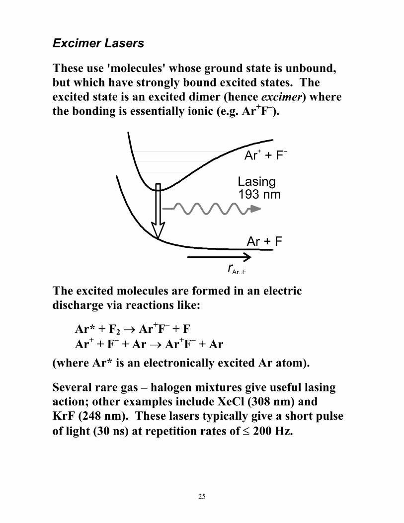
Excimer Lasers

These use 'molecules' whose ground state is unbound, but which have strongly bound excited states. The excited state is an excited dimer (hence excimer) where the bonding is essentially ionic (e.g. Ar+F–).

The excited molecules are formed in an electric discharge via reactions like:

Ar* + F2 → Ar+F– + F Ar+ + F– + Ar → Ar+F– + Ar

(where Ar* is an electronically excited Ar atom). Several rare gas – halogen mixtures give useful lasing action; other examples include XeCl (308 nm) and KrF (248 nm). These lasers typically give a short pulse of light (30 ns) at repetition rates of ≤ 200 Hz.

26

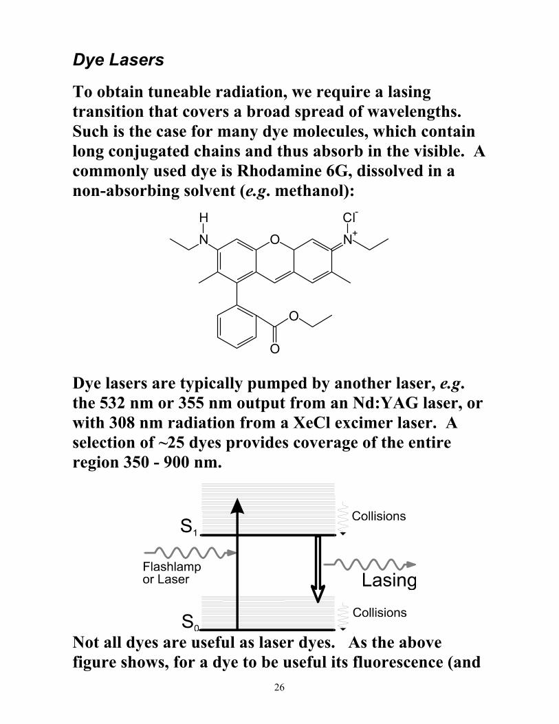
Dye Lasers

To obtain tuneable radiation, we require a lasing transition that covers a broad spread of wavelengths. Such is the case for many dye molecules, which contain long conjugated chains and thus absorb in the visible. A commonly used dye is Rhodamine 6G, dissolved in a non-absorbing solvent (e.g. methanol):

N O N+

O

O

Cl-H

Dye lasers are typically pumped by another laser, e.g. the 532 nm or 355 nm output from an Nd:YAG laser, or with 308 nm radiation from a XeCl excimer laser. A selection of ~25 dyes provides coverage of the entire region 350 - 900 nm.

Not all dyes are useful as laser dyes. As the above figure shows, for a dye to be useful its fluorescence (and

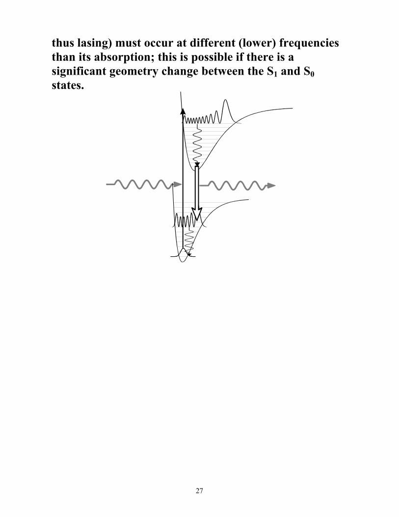
27

thus lasing) must occur at different (lower) frequencies than its absorption; this is possible if there is a significant geometry change between the S1 and S0 states.

28

Laser Applications

Laser Spectroscopy In principle, a laser can be used in a straightforward absorption experiment, i.e.

Tunable laser → Sample → Detector c.f. the teaching lab. spectrometers you have used, though these use a white light source and select the required wavelength with a prism or grating.

A laser gives the advantages of higher resolution, sensitivity, and long path lengths.

Direct absorption measurements like these are limited by detector noise (particularly for conventional spectrometers) and fluctuations in the light source (normally the limiting factor in laser absorption). Because it is difficult to measure small changes in a large signal, absorption measurements are rarely the method of choice for laser spectroscopy. The smallest change in intensity that can be measured is typically ~10–5 of the incident light. (But note cavity ring down spectroscopy http://www.chm.bris.ac.uk/pt/laser/laserhom.htm)

Greater sensitivity can often be obtained by measuring a side-effect produced by the absorption of light, rather than the loss of light itself. Such methods can detect changes equivalent to the absorption of the order of 10–17 of the incident light!

29

Laser Induced Fluorescence (LIF) The spontaneous fluorescence from excited molecules can be detected in a very sensitive manner as the signal off-resonance is very small - the noise level of the best detectors is just a few photons/sec.

This means only a few molecules need be excited and concentrations as low as 100 molecules/cm3 (=10–19 M) can be detected. This makes LIF a method of choice for electronic spectroscopy. The technique does have some limitations, however: 1. Scattered laser light (e.g. from dust particles, imperfections in windows) 2. Fluorescence may be quenched (recall possible fates of excited state molecules: (pre)dissociation, IC, ISC, collisional energy transfer) 3. Absorption and LIF spectra may not be identical. 4. Not useful when spontaneous fluorescence is slow. Given the ν3 factor in A, this means that infra-red spectra cannot be taken this way. (IR detectors are also relatively insensitive.)

LIF is well suited for use with small localised samples (e.g. jet-cooled molecular species, including free radicals, in a supersonic beam), and for spatially resolved concentration profiling. (see http://www.chm.bris.ac.uk/pt/western/cmwspec.html)

30

Laser Identification, Detection and Ranging, LIDAR

Remote sensing of, e.g., pollutant emission from a chimney is possible by firing a laser into the sky and collecting light coming back from the laser beam from fluorescence, the Raman effect or scattering from dust particles. Analysis of this light enables identification of the species present, their concentrations and their positions (from the time delay).

Multiphoton Spectroscopy

In sufficiently intense radiation fields molecules can absorb more than one photon at once, giving a resonance condition ∆E = nhν rather than the usual ∆E = hν. Two photon absorption can be viewed as a two step process in which a virtual state comprising a molecule + a photon is prepared. This lasts only as long as the photon takes to pass the molecule. Absorption then takes place from the virtual state. Raman spectroscopy can be viewed in a similar way, i.e. as (spontaneous) emission from a virtual state, and has analogous selection rules.

Virtual State

A

B

Multiphoton processes are inherently improbable. The table below shows the fraction of molecules excited for a

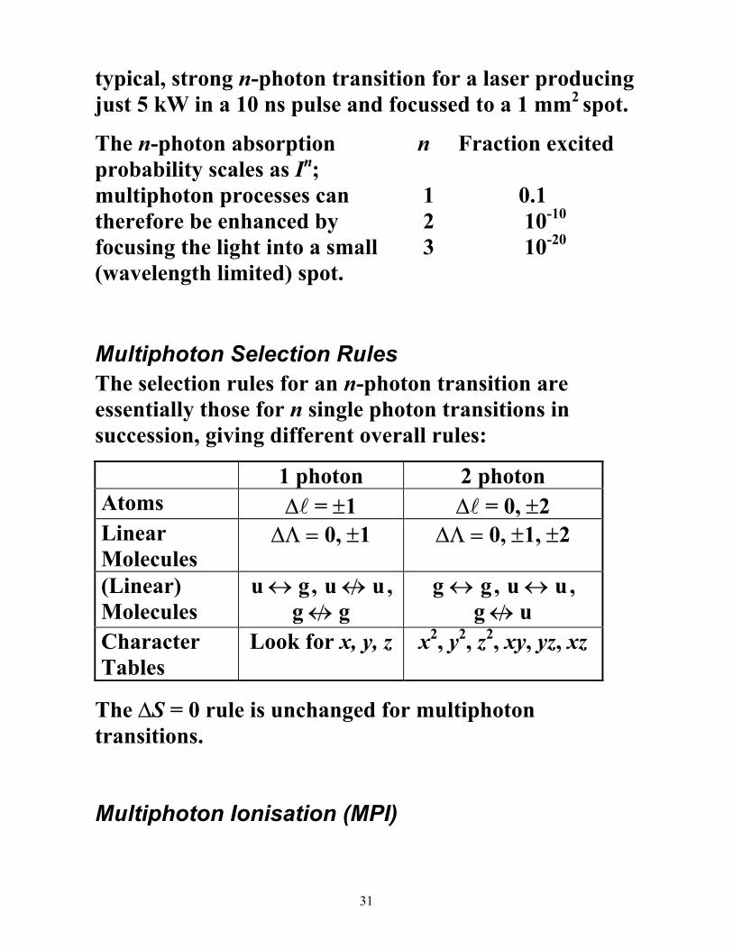
31

typical, strong n-photon transition for a laser producing just 5 kW in a 10 ns pulse and focussed to a 1 mm2 spot.

The n-photon absorption probability scales as In; multiphoton processes can therefore be enhanced by focusing the light into a small (wavelength limited) spot.

n Fraction excited 1 0.1 2 10-10

3 10-20

Multiphoton Selection Rules The selection rules for an n-photon transition are essentially those for n single photon transitions in succession, giving different overall rules:

1 photon 2 photon Atoms ∆l = ±1 ∆l = 0, ±2 Linear Molecules

∆Λ = 0, ±1 ∆Λ = 0, ±1, ±2

(Linear) Molecules

u g↔ , u u/↔ , g g/↔

g g↔ , u u↔ , g u/↔

Character Tables

Look for x, y, z x2, y2, z2, xy, yz, xz

The ∆S = 0 rule is unchanged for multiphoton transitions. Multiphoton Ionisation (MPI)

32

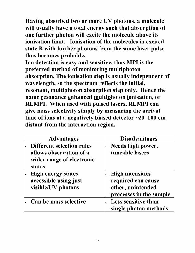
Having absorbed two or more UV photons, a molecule will usually have a total energy such that absorption of one further photon will excite the molecule above its ionisation limit. Ionisation of the molecules in excited state B with further photons from the same laser pulse thus becomes probable. Ion detection is easy and sensitive, thus MPI is the preferred method of monitoring multiphoton absorption. The ionisation step is usually independent of wavelength, so the spectrum reflects the initial, resonant, multiphoton absorption step only. Hence the name resonance enhanced multiphoton ionisation, or REMPI. When used with pulsed lasers, REMPI can give mass selectivity simply by measuring the arrival time of ions at a negatively biased detector ~20–100 cm distant from the interaction region.

Advantages Disadvantages • Different selection rules

allows observation of a wider range of electronic states

• Needs high power, tuneable lasers

• High energy states accessible using just visible/UV photons

• High intensities required can cause other, unintended processes in the sample

• Can be mass selective • Less sensitive than single photon methods

33

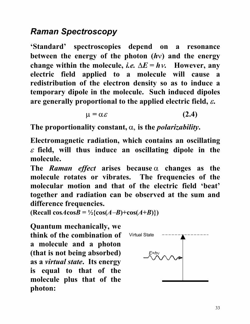
Raman Spectroscopy

‘Standard’ spectroscopies depend on a resonance between the energy of the photon (hν) and the energy change within the molecule, i.e. ∆E = hν. However, any electric field applied to a molecule will cause a redistribution of the electron density so as to induce a temporary dipole in the molecule. Such induced dipoles are generally proportional to the applied electric field, ε.

µ = αε (2.4)

The proportionality constant, α, is the polarizability.

Electromagnetic radiation, which contains an oscillating ε field, will thus induce an oscillating dipole in the molecule. The Raman effect arises because α changes as the molecule rotates or vibrates. The frequencies of the molecular motion and that of the electric field ‘beat’ together and radiation can be observed at the sum and difference frequencies. (Recall cosAcosB = ½cos(A−B)+cos(A+B))

Quantum mechanically, we think of the combination of a molecule and a photon (that is not being absorbed) as a virtual state. Its energy is equal to that of the molecule plus that of the photon:

Virtual State

E=hν

34

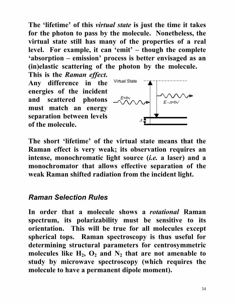
The ‘lifetime’ of this virtual state is just the time it takes for the photon to pass by the molecule. Nonetheless, the virtual state still has many of the properties of a real level. For example, it can ‘emit’ – though the complete ‘absorption – emission’ process is better envisaged as an (in)elastic scattering of the photon by the molecule. This is the Raman effect. Any difference in the energies of the incident and scattered photons must match an energy separation between levels of the molecule.

Virtual State

E=hν E−∆=hν’

∆

The short ‘lifetime’ of the virtual state means that the Raman effect is very weak; its observation requires an intense, monochromatic light source (i.e. a laser) and a monochromator that allows effective separation of the weak Raman shifted radiation from the incident light.

Raman Selection Rules

In order that a molecule shows a rotational Raman spectrum, its polarizability must be sensitive to its orientation. This will be true for all molecules except spherical tops. Raman spectroscopy is thus useful for determining structural parameters for centrosymmetric molecules like H2, O2 and N2 that are not amenable to study by microwave spectroscopy (which requires the molecule to have a permanent dipole moment).

35

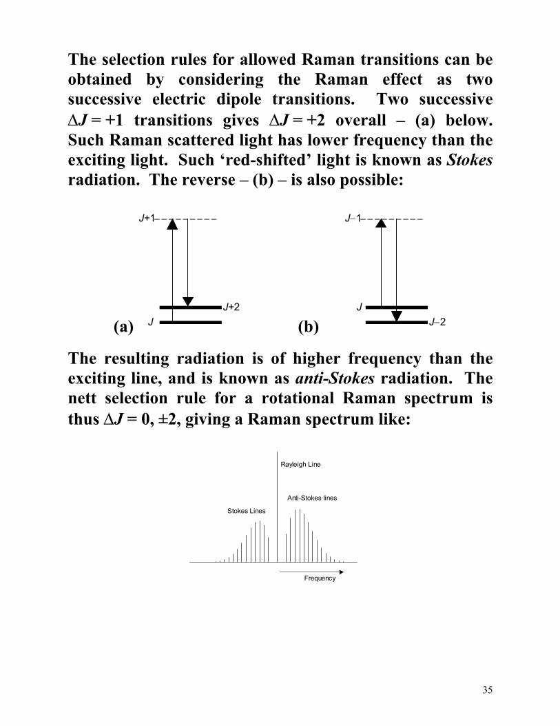
The selection rules for allowed Raman transitions can be obtained by considering the Raman effect as two successive electric dipole transitions. Two successive ∆J = +1 transitions gives ∆J = +2 overall – (a) below. Such Raman scattered light has lower frequency than the exciting light. Such ‘red-shifted’ light is known as Stokes radiation. The reverse – (b) – is also possible:

(a) J

J+1

J+2

(b)

J

J−1

J−2

The resulting radiation is of higher frequency than the exciting line, and is known as anti-Stokes radiation. The nett selection rule for a rotational Raman spectrum is thus ∆J = 0, ±2, giving a Raman spectrum like:

Frequency

Stokes Lines

Anti-Stokes lines

Rayleigh Line

36

The intense central feature, the Rayleigh line, typically dominates the spectrum. This light has been scattered by the molecule but not changed in frequency.

We can apply similar logic to determine the selection rules for allowed vibrational Raman transitions. For any given molecule, the allowed one-photon (infrared) transitions transform in the same way as x¸ y and z in the relevant character table. Allowed vibrational Raman transitions must have the symmetry of one of the possible combinations (products) of x¸ y and z, i.e. xy, xz, yz, x2, y2 and z2. This leads to the mutual exclusion principle which states that, for molecules with a centre of symmetry, no vibrational modes can be both IR and Raman active. (This follows because x, y and z always have u symmetry so their products must always have g symmetry. The analogy with the selection rules for 2-photon absorption should be obvious.)

Additional information can be gleaned from Raman spectra excited with plane (or linearly) polarized light, i.e. with ε oscillating in one plane. (Most laser radiation is plane polarised). • Features in Raman spectra that show the same

polarization as the exciting light are associated with totally symmetric vibrational modes.

• All other Raman active vibrations show (at least some) loss of polarization, or depolarization.

37

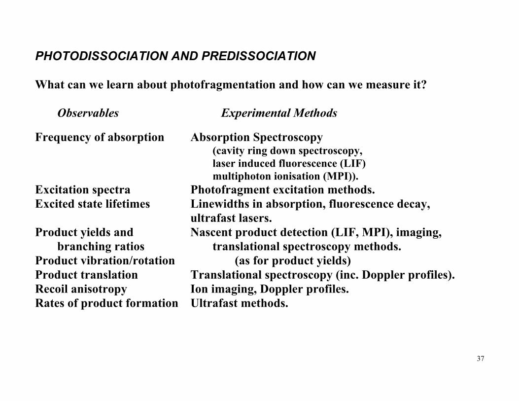
PHOTODISSOCIATION AND PREDISSOCIATION What can we learn about photofragmentation and how can we measure it? Observables Experimental Methods Frequency of absorption Absorption Spectroscopy (cavity ring down spectroscopy, laser induced fluorescence (LIF) multiphoton ionisation (MPI)). Excitation spectra Photofragment excitation methods. Excited state lifetimes Linewidths in absorption, fluorescence decay, ultrafast lasers. Product yields and Nascent product detection (LIF, MPI), imaging, branching ratios translational spectroscopy methods. Product vibration/rotation (as for product yields) Product translation Translational spectroscopy (inc. Doppler profiles). Recoil anisotropy Ion imaging, Doppler profiles. Rates of product formation Ultrafast methods.

38

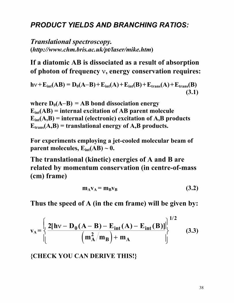
PRODUCT YIELDS AND BRANCHING RATIOS: Translational spectroscopy. (http://www.chm.bris.ac.uk/pt/laser/mike.htm)

If a diatomic AB is dissociated as a result of absorption of photon of frequency ν, energy conservation requires:

hν + Eint(AB) = D0(A−B) + Eint(A) + Eint(B) + Etrans(A) + Etrans(B) (3.1)

where D0(A−B) = AB bond dissociation energy Eint(AB) = internal excitation of AB parent molecule Eint(A,B) = internal (electronic) excitation of A,B products Etrans(A,B) = translational energy of A,B products. For experiments employing a jet-cooled molecular beam of parent molecules, Eint(AB) ~ 0.

The translational (kinetic) energies of A and B are related by momentum conservation (in centre-of-mass (cm) frame)

mAvA = mBvB (3.2) Thus the speed of A (in the cm frame) will be given by:

vA = ( )2 0

2

1 2[ ( ) ( ) ( )]int int

/h D A B E A E B

m m mA B A

ν − − − −

+

(3.3)

CHECK YOU CAN DERIVE THIS!

39

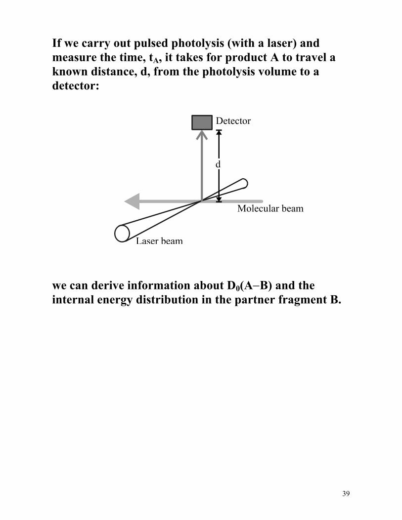
If we carry out pulsed photolysis (with a laser) and measure the time, tA, it takes for product A to travel a known distance, d, from the photolysis volume to a detector: we can derive information about D0(A−B) and the internal energy distribution in the partner fragment B.

40

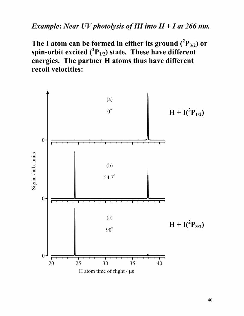
Example: Near UV photolysis of HI into H + I at 266 nm. The I atom can be formed in either its ground (2P3/2) or spin-orbit excited (2P1/2) state. These have different energies. The partner H atoms thus have different recoil velocities:

H + I(2P1/2) H + I(2P3/2)

41

• Early time peak is associated with H + I(2P3/2) products vH = 17.6 km/s. • Analysis gives D0(H−I) = 24630 ± 20 cm-1. • Note that relative areas of the fast and slow peaks vary with θ, the angle between the electric vector of the photolysis light and the axis along which the recoiling H atoms are detected. • Analysis indicates that ~52% of the I atoms formed in the 266 nm photolysis of HI are formed in their excited (2P1/2) spin-orbit state. Doppler spectroscopy can yield the same information. An H atom (or any atom or molecule) at rest will absorb radiation at a frequency ν0 corresponding to the line centre of the transition between two of its quantum states. The effect of motion along the propagation axis of the probe radiation, z, (with velocity component vz) is to shift the frequency of absorption to a new frequency ν given by:

ν = ν0 1±

vcz . (3.4)

The +/− corresponds to motion respectively parallel and anti-parallel to the propagation direction of the probe radiation. ∆ν = ν − ν0 = ±ν0vz/c is called the Doppler shift (recall p. 9)

42

Doppler profile for H atoms from the 266 nm photolysis of HI The Doppler profile of the H atoms resulting from HI photolysis at 266 nm can be divided into two components, one wider (i.e. bigger Doppler shift, ∴ faster, associated with H + I(2P3/2) products) than the other (associated with H + I(2P1/2) products).

Note: the two profiles have different shapes.

This, like the observation that the relative intensities of the two peaks in the H atom TOF spectrum depends on the relative orientation of the laser polarisation axis and the detector axis, reflects the fact that the distribution of fragment recoil velocities is anisotropic.

43

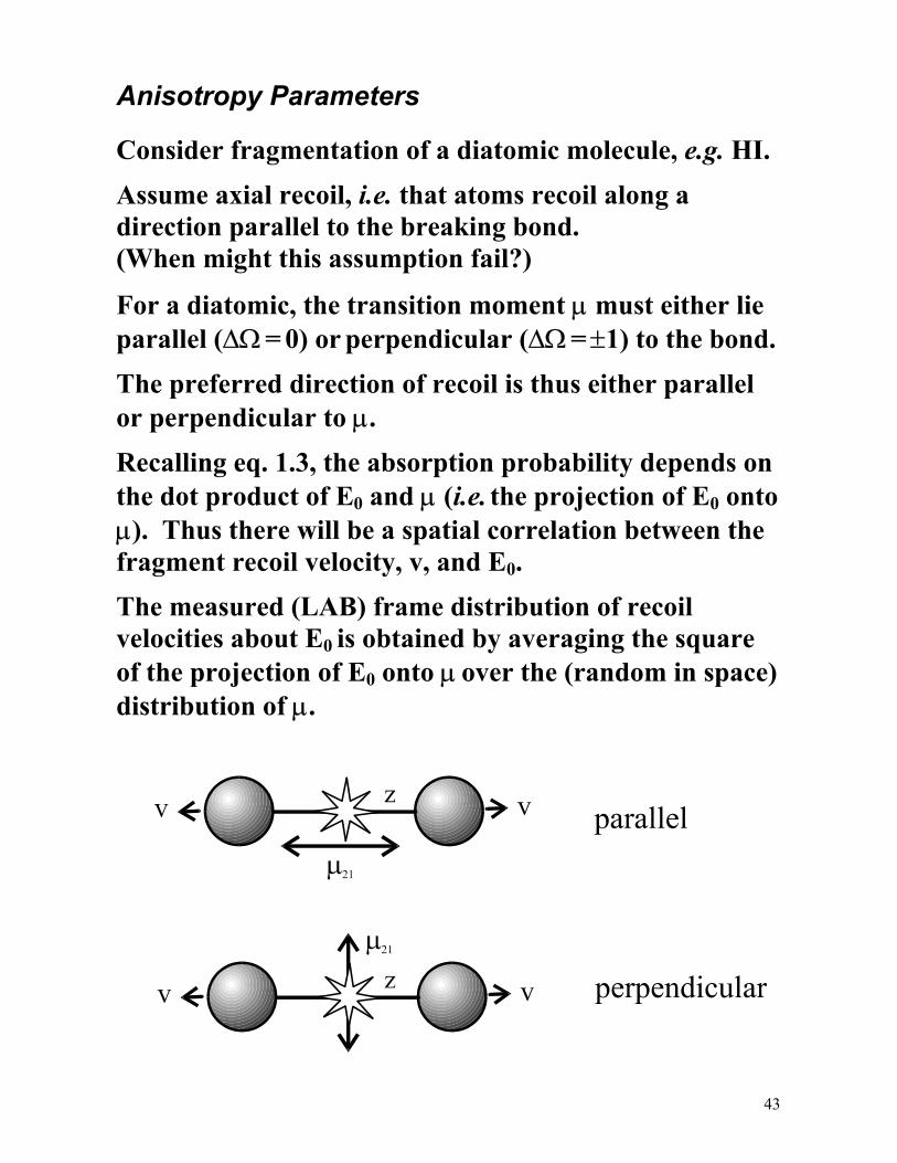
Anisotropy Parameters Consider fragmentation of a diatomic molecule, e.g. HI.

Assume axial recoil, i.e. that atoms recoil along a direction parallel to the breaking bond. (When might this assumption fail?)

For a diatomic, the transition moment µ must either lie parallel (∆Ω = 0) or perpendicular (∆Ω = ±1) to the bond.

The preferred direction of recoil is thus either parallel or perpendicular to µ.

Recalling eq. 1.3, the absorption probability depends on the dot product of E0 and µ (i.e. the projection of E0 onto µ). Thus there will be a spatial correlation between the fragment recoil velocity, v, and E0.

The measured (LAB) frame distribution of recoil velocities about E0 is obtained by averaging the square of the projection of E0 onto µ over the (random in space) distribution of µ.

44

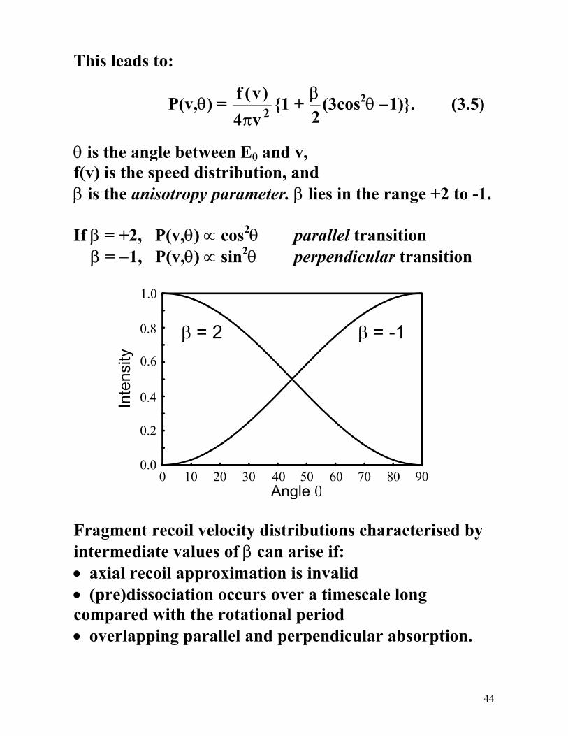
This leads to:

P(v,θ) = f vv

( )4 2π

1 + β2

(3cos2θ −1). (3.5)

θ is the angle between E0 and v, f(v) is the speed distribution, and β is the anisotropy parameter. β lies in the range +2 to -1. If β = +2, P(v,θ) ∝ cos2θ parallel transition β = −1, P(v,θ) ∝ sin2θ perpendicular transition

Fragment recoil velocity distributions characterised by intermediate values of β can arise if: • axial recoil approximation is invalid • (pre)dissociation occurs over a timescale long compared with the rotational period • overlapping parallel and perpendicular absorption.

45

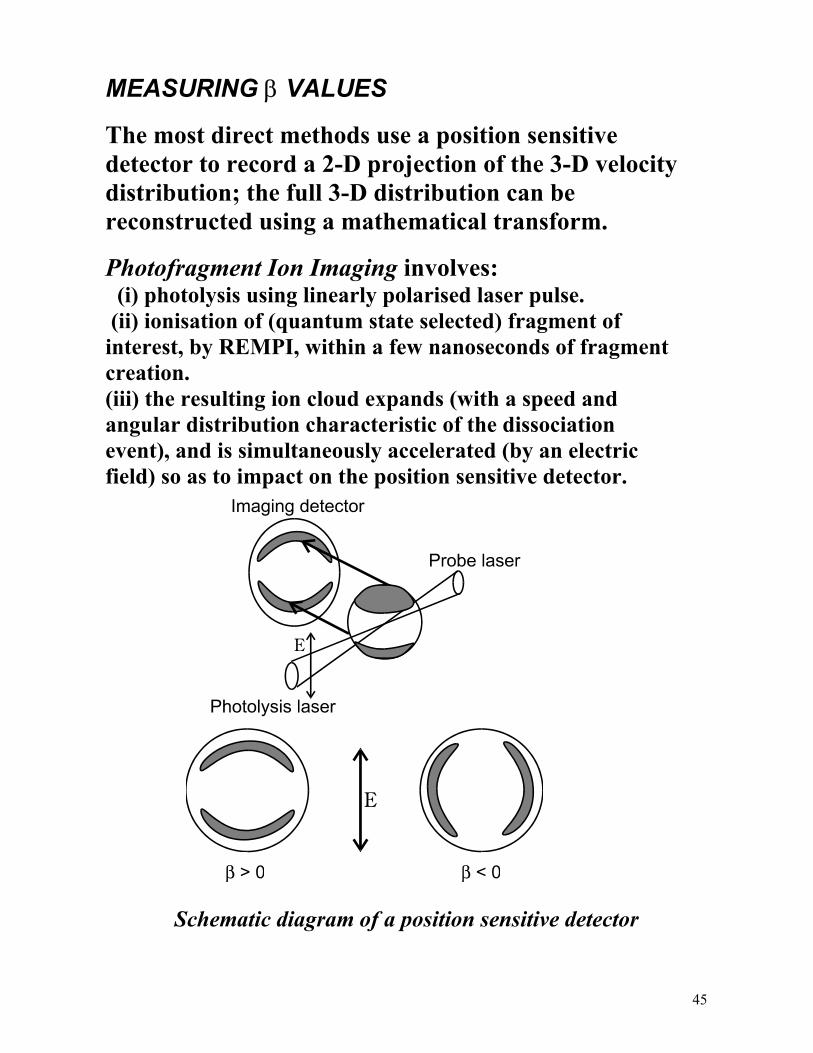
MEASURING β VALUES

The most direct methods use a position sensitive detector to record a 2-D projection of the 3-D velocity distribution; the full 3-D distribution can be reconstructed using a mathematical transform.

Photofragment Ion Imaging involves: (i) photolysis using linearly polarised laser pulse. (ii) ionisation of (quantum state selected) fragment of interest, by REMPI, within a few nanoseconds of fragment creation. (iii) the resulting ion cloud expands (with a speed and angular distribution characteristic of the dissociation event), and is simultaneously accelerated (by an electric field) so as to impact on the position sensitive detector.

Schematic diagram of a position sensitive detector

46

Image of the H atoms from 266 nm photolysis of HI:

The same recoil anisotropy also reveals itself in the different Doppler profiles of the fast and slow H atoms arising in this photolysis.

Idealised Doppler profiles for fragments following photodissociation with different values of β. The forms shown are appropriate for colinear photolysis and probe laser beams.

47

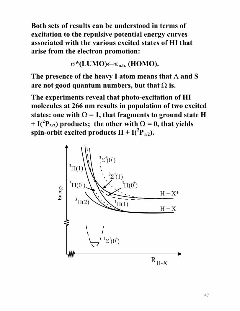
Both sets of results can be understood in terms of excitation to the repulsive potential energy curves associated with the various excited states of HI that arise from the electron promotion:

σ*(LUMO)←πn.b. (HOMO).

The presence of the heavy I atom means that Λ and S are not good quantum numbers, but that Ω is.

The experiments reveal that photo-excitation of HI molecules at 266 nm results in population of two excited states: one with Ω = 1, that fragments to ground state H + I(2P3/2) products; the other with Ω = 0, that yields spin-orbit excited products H + I(2P1/2).

48

OZONE PHOTOCHEMISTRY

Pivotal to stratospheric chemistry is the creation and destruction of the ozone layer, which protects the Earth's surface and everything on it from all harmful solar radiation in the wavelength range 240 - 310 nm. (AJO-E lectures, Level 2)

O3 is produced by O2 photolysis at λ < 242 nm:

O2 + hν → 2 O (4.1)

O + O2 + M → O3 + M (4.2)

[O3] is limited by two further reactions:

O3 + hν → O + O2 (4.3)

O + O3 → 2 O2 (4.4)

(4.1) - (4.4) constitute the Chapman scheme.

Species like Cl, NO, H, OH (henceforth X) provide an alternative path for reaction (4.4):

X + O3 → XO + O2 (4.5)

XO + O → X + O2 (4.6)

X acts as a catalyst.

49

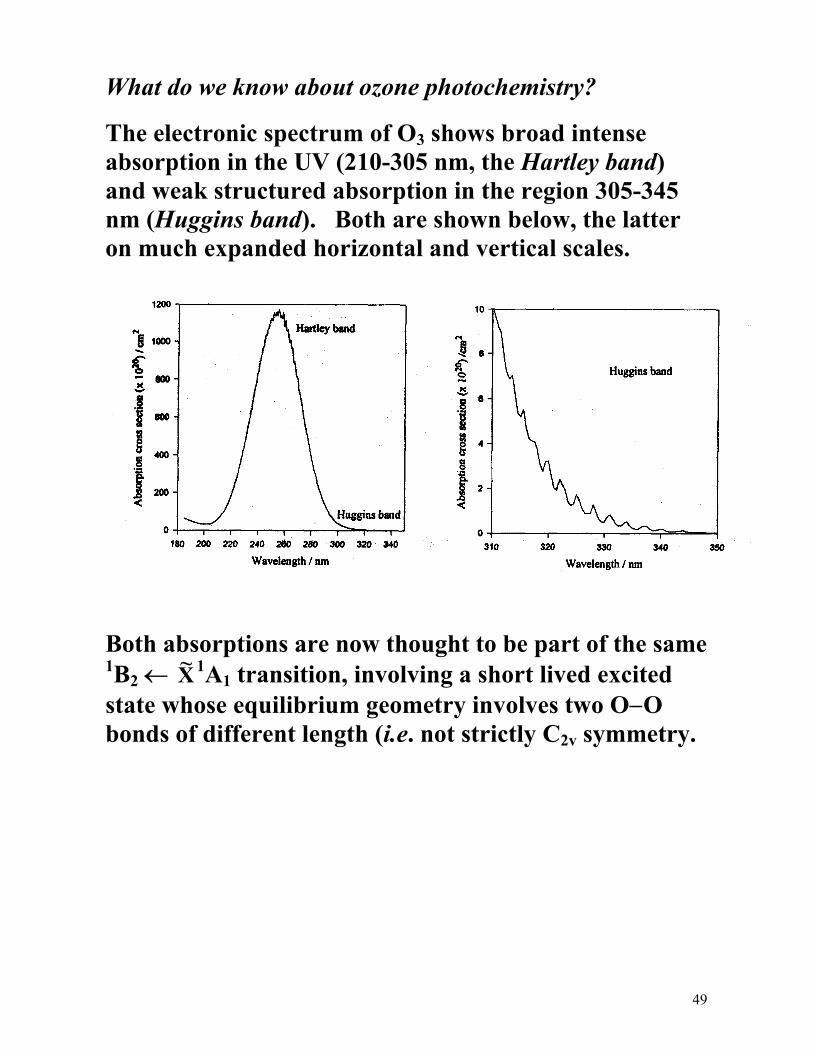
What do we know about ozone photochemistry?

The electronic spectrum of O3 shows broad intense absorption in the UV (210-305 nm, the Hartley band) and weak structured absorption in the region 305-345 nm (Huggins band). Both are shown below, the latter on much expanded horizontal and vertical scales.

Both absorptions are now thought to be part of the same 1B2 ← ~X 1A1 transition, involving a short lived excited state whose equilibrium geometry involves two O−O bonds of different length (i.e. not strictly C2v symmetry.

50

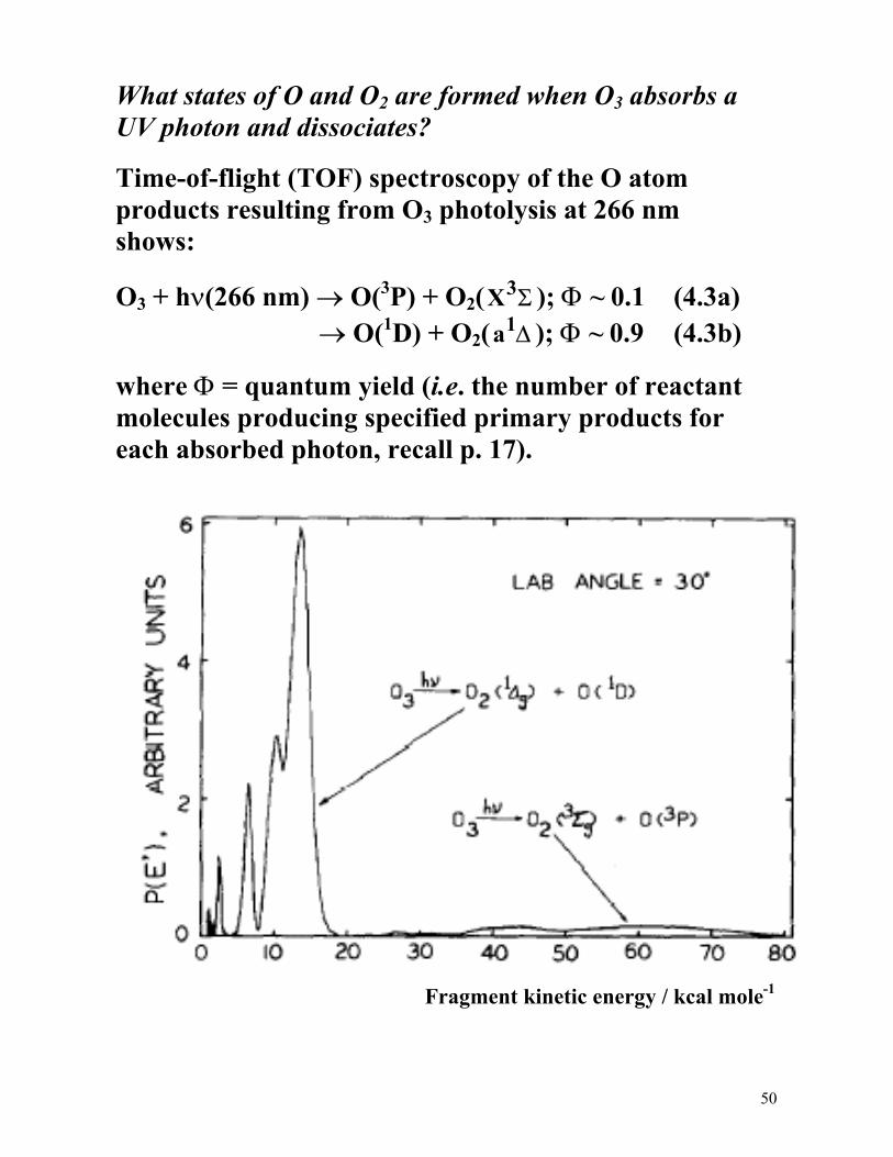
What states of O and O2 are formed when O3 absorbs a UV photon and dissociates?

Time-of-flight (TOF) spectroscopy of the O atom products resulting from O3 photolysis at 266 nm shows:

O3 + hν(266 nm) → O(3P) + O2(X3Σ ); Φ ~ 0.1 (4.3a) → O(1D) + O2(a1∆ ); Φ ~ 0.9 (4.3b)

where Φ = quantum yield (i.e. the number of reactant molecules producing specified primary products for each absorbed photon, recall p. 17).

Fragment kinetic energy / kcal mole-1

51

Note that both (4.3a) and (4.3b) are spin-allowed if we assume that dissociation occurs from a singlet excited state. The alternative possibilities, i.e.

O3 + hν → O(3P) + O2(a1∆ ) (4.3c) → O(1D) + O2(X3Σ ), (4.3d)

though both energetically allowed following UV excitation, would be spin-forbidden.

__________________________ Ozone is topical because of: • the well documented Antarctic ozone hole and the general thinning of the ozone layer due to Cl catalysed variants of (4.5) and (4.6), and • increasing levels of ground level O3 associated with photochemical smog. At the more fundamental level there have been two longstanding questions regarding ozone concentrations and its role in the atmosphere.

52

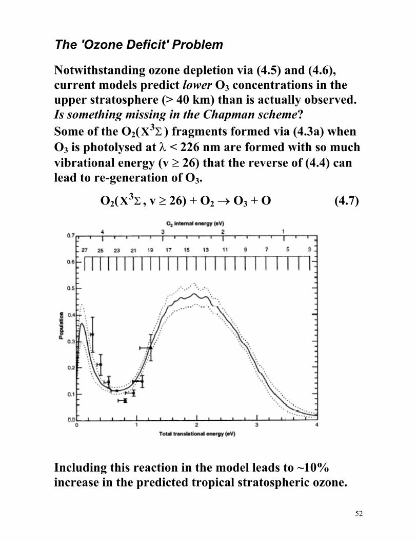
The 'Ozone Deficit' Problem

Notwithstanding ozone depletion via (4.5) and (4.6), current models predict lower O3 concentrations in the upper stratosphere (> 40 km) than is actually observed. Is something missing in the Chapman scheme? Some of the O2(X3Σ ) fragments formed via (4.3a) when O3 is photolysed at λ < 226 nm are formed with so much vibrational energy (v ≥ 26) that the reverse of (4.4) can lead to re-generation of O3.

O2(X3Σ , v ≥ 26) + O2 → O3 + O (4.7)

Including this reaction in the model leads to ~10% increase in the predicted tropical stratospheric ozone.

53

Tropospheric Ozone Ozone in the troposphere is a pollutant and one of the major components of photochemical smog.

Tropospheric ozone arises primarily from NO2 photolysis:

NO2 + hν (λ < 400 nm) → NO + O(3P) (4.8)

O + O2 + M → O3 + M (4.9)

NO + O3 → NO2 + O2 (4.10) Invoking the steady state approximation to both O atoms and O3 and solving for [O3] yields:

[O3] = k NOk NO

4 8 2

4 10

.

.

[ ][ ]

(Check you can do this!)

54

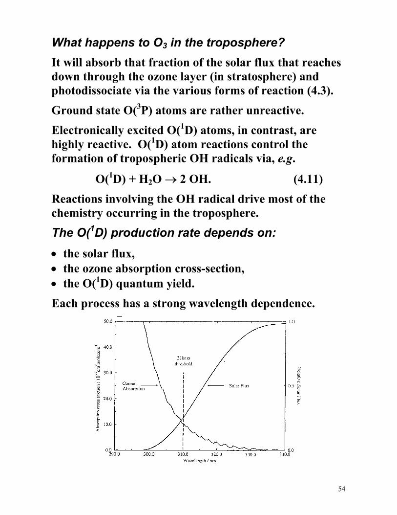
What happens to O3 in the troposphere?

It will absorb that fraction of the solar flux that reaches down through the ozone layer (in stratosphere) and photodissociate via the various forms of reaction (4.3).

Ground state O(3P) atoms are rather unreactive.

Electronically excited O(1D) atoms, in contrast, are highly reactive. O(1D) atom reactions control the formation of tropospheric OH radicals via, e.g.

O(1D) + H2O → 2 OH. (4.11)

Reactions involving the OH radical drive most of the chemistry occurring in the troposphere.

The O(1D) production rate depends on:

• the solar flux, • the ozone absorption cross-section, • the O(1D) quantum yield.

Each process has a strong wavelength dependence.

55

How does Φ(O(1D)) vary with wavelength?

We have already seen that it has a value of ~0.9 at λ = 266 nm, and that the partner fragment is the spin-allowed product O2(a1∆ ) - eq. (4.3b).

Φ(O(1D)) – the vertical axis of the plot below – has a value of ~0.9 at all photolysis wavelengths λ ≤ 310 nm, which corresponds to the energetic threshold for reaction (4.3b).

At longer wavelengths Φ(O(1D)) falls dramatically, but not to zero as NASA recommend (1994) in their database for stratospheric ozone modelling. Why?

56

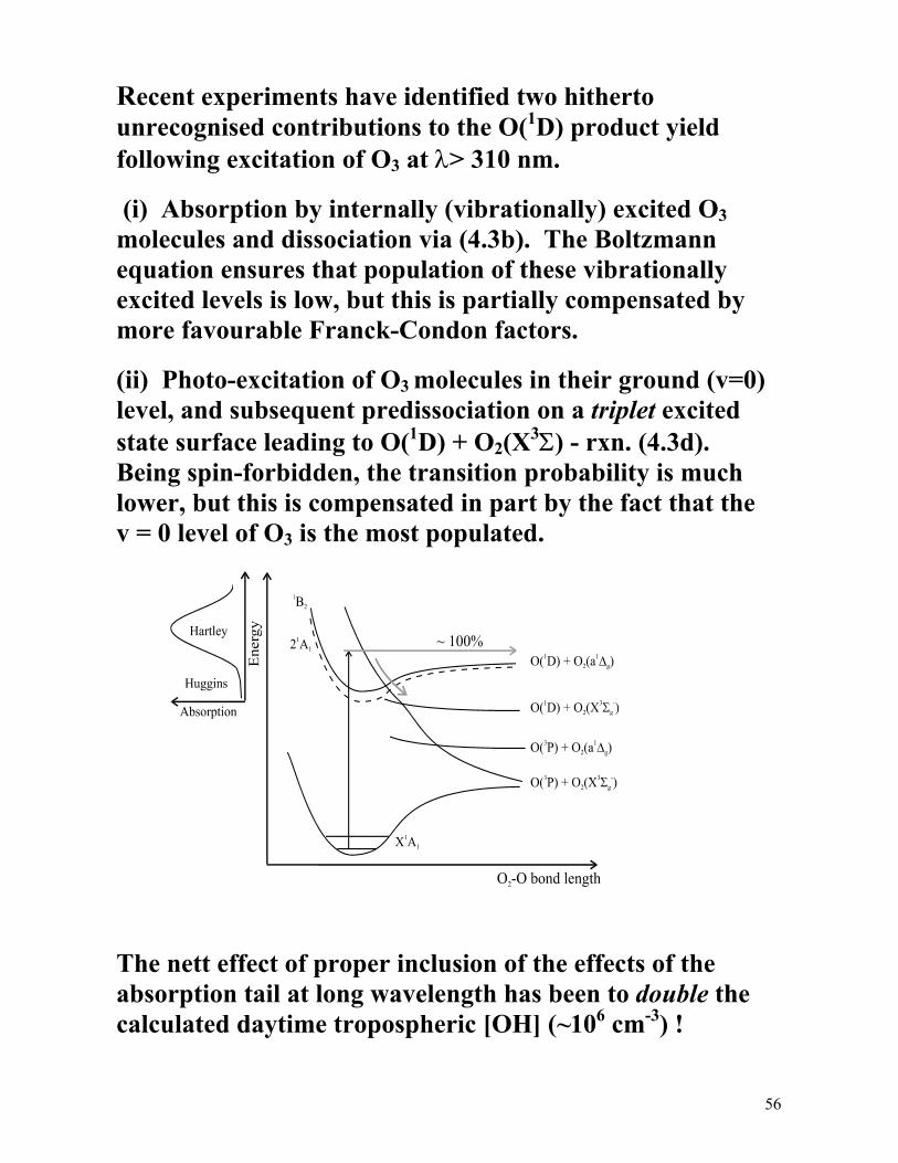
Recent experiments have identified two hitherto unrecognised contributions to the O(1D) product yield following excitation of O3 at λ> 310 nm.

(i) Absorption by internally (vibrationally) excited O3 molecules and dissociation via (4.3b). The Boltzmann equation ensures that population of these vibrationally excited levels is low, but this is partially compensated by more favourable Franck-Condon factors.

(ii) Photo-excitation of O3 molecules in their ground (v=0) level, and subsequent predissociation on a triplet excited state surface leading to O(1D) + O2(X3Σ) - rxn. (4.3d). Being spin-forbidden, the transition probability is much lower, but this is compensated in part by the fact that the v = 0 level of O3 is the most populated.

The nett effect of proper inclusion of the effects of the absorption tail at long wavelength has been to double the calculated daytime tropospheric [OH] (~106 cm-3) !

57

FEMTOCHEMISTRY

Questions.

• On what timescale does a molecule dissociate once it has absorbed a photon and been excited to an unstable electronically excited state?

• How does the molecular geometry distort during this dissociation process?

• Can we use some property of a light pulse (frequency, phase) to control the way in which a molecule fragments, or a reaction proceeds?

We can obtain an idea of the timescales by assuming that the evolution from excited molecule to products involves the internuclear separations changing by ~ 0.2 nm, and that the atoms are moving at ~ 103

m s-1, i.e. the process takes ~ 10-13 s.

To investigate the evolution from reactants to products we need to be able to interrogate the system several times within this period, i.e. we require femtosecond (10-15 s) time resolution.

From the energy-time form of the Uncertainty Principle

∆E.∆t ~ h ⇒ ∆ν.∆t ~ 1/2π . (1.14 again)

A 100 fs laser pulse will have a frequency uncertainty (full width half maximum) of (at least) 1.6 x 1012 s-1, or >52 cm-1. It is only 30 µm long, and very delicate!

58

When thinking about molecular excitations using such pulses it is customary to use time dependent quantum mechanics, and to think in terms of wavepackets - a superposition of stationary state wavefunctions with a well defined initial phase relationship to each other.

It is simplest to concentrate on unimolecular processes, e.g. photodissociation. We could answer the posed questions, in principle, by exciting the molecules with a very short pulse of light and looking at the emission from molecules in the act of dissociation.

Wave packet propagation describing photofragmentation. The laser photon transfers the ground state wavefunction to the excited state at t0. During fragmentation, an excited ABC molecule could fluoresce to various vibrational levels of the ground state. The spectrum of this emission (bottom left) consists of a series of broadened bands spaced according to the ground state vibrational levels.

59

Unfortunately, the quantum yield of such emission

Φ = kemission /kdissociation ~ 107 s-1/ 1013 s-1 ~ 10-6

(recall eq. 1.15) is so low as to be barely detectable.

It would be much better to use two short laser pulses, one to excite the parent molecule, the second (after a well defined time delay) to probe loss of the parent and/or product build up. Pump-probe experiments of this type are now performed. Consider two examples:

1. ICN + hν (~307 nm) → I + CN

2. NaI + hν (~310 nm) → Na + I

(The monitored species in each case is underlined).

Both studies employed ~40 fs pump and probe laser pulses. The excitation bandwidth is ~1.2 nm (~130 cm-1 FWHM).

60

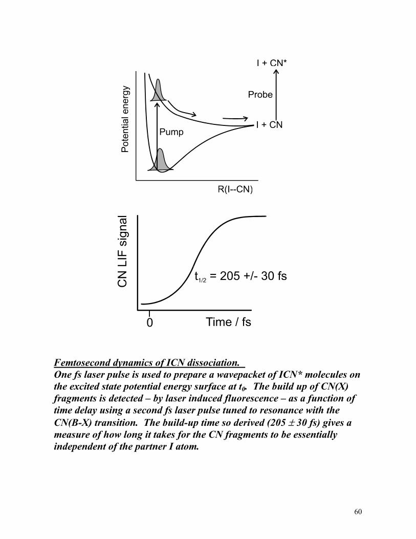
Femtosecond dynamics of ICN dissociation. One fs laser pulse is used to prepare a wavepacket of ICN* molecules on the excited state potential energy surface at t0. The build up of CN(X) fragments is detected – by laser induced fluorescence – as a function of time delay using a second fs laser pulse tuned to resonance with the CN(B-X) transition. The build-up time so derived (205 ± 30 fs) gives a measure of how long it takes for the CN fragments to be essentially independent of the partner I atom.

61

Femtosecond dynamics of NaI dissociation. Bottom: experimental observations of wave packet motion, made by detecting the activated [NaI]*# complexes or the free Na atoms. Top: PE curves (left) and QM calculations (right) showing the wavepacket as it evolves in time and space. The corresponding changes in bond character are also noted: covalent (at 160 fs), covalent/ionic (at 500 fs) and back to covalent (at 1.3 ps). ( from Zewail, J. Phys. Chem. 100, 12701, (1996)).

62

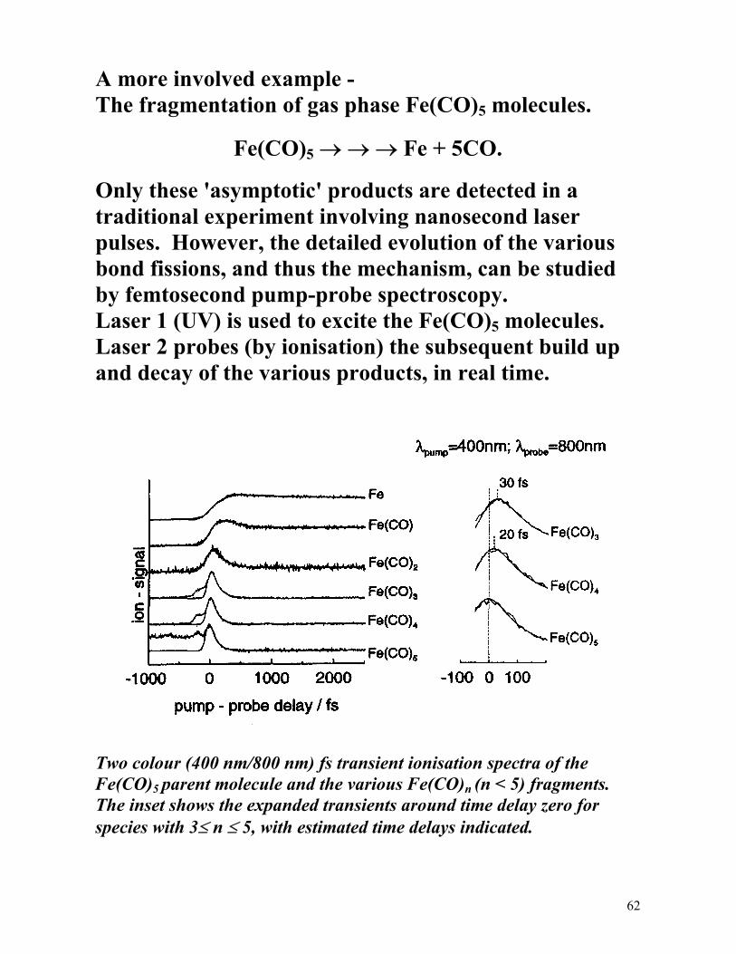
A more involved example - The fragmentation of gas phase Fe(CO)5 molecules.

Fe(CO)5 → → → Fe + 5CO.

Only these 'asymptotic' products are detected in a traditional experiment involving nanosecond laser pulses. However, the detailed evolution of the various bond fissions, and thus the mechanism, can be studied by femtosecond pump-probe spectroscopy. Laser 1 (UV) is used to excite the Fe(CO)5 molecules. Laser 2 probes (by ionisation) the subsequent build up and decay of the various products, in real time.

Two colour (400 nm/800 nm) fs transient ionisation spectra of the Fe(CO)5 parent molecule and the various Fe(CO)n (n < 5) fragments. The inset shows the expanded transients around time delay zero for species with 3≤ n ≤ 5, with estimated time delays indicated.

63

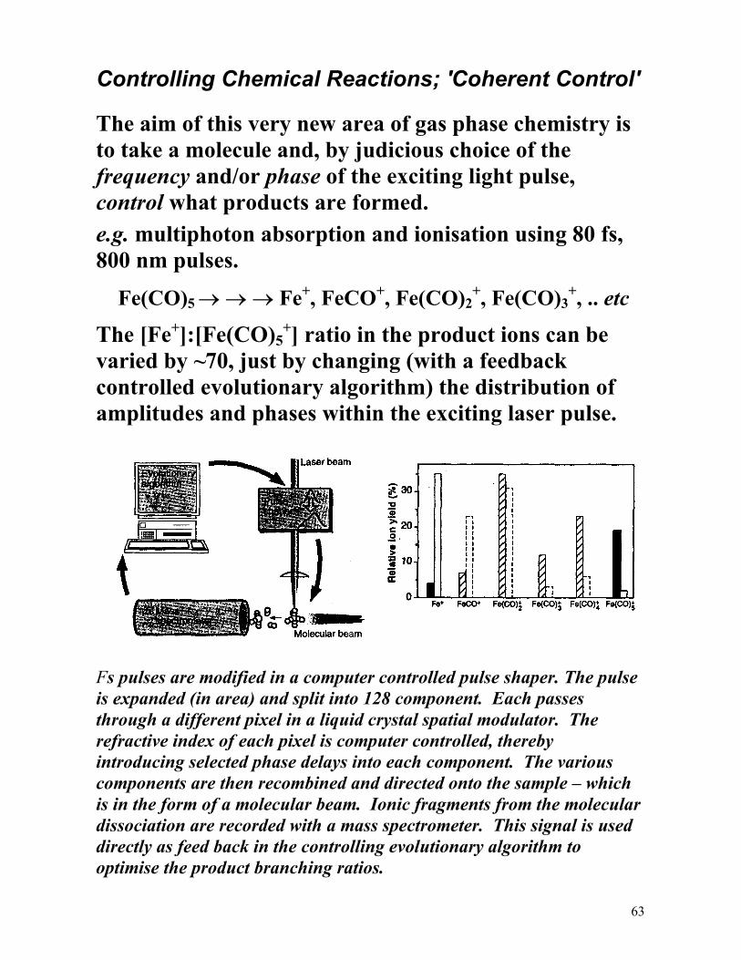
Controlling Chemical Reactions; 'Coherent Control' The aim of this very new area of gas phase chemistry is to take a molecule and, by judicious choice of the frequency and/or phase of the exciting light pulse, control what products are formed.

e.g. multiphoton absorption and ionisation using 80 fs, 800 nm pulses.

Fe(CO)5 → → → Fe+, FeCO+, Fe(CO)2+, Fe(CO)3

+, .. etc

The [Fe+]:[Fe(CO)5+] ratio in the product ions can be

varied by ~70, just by changing (with a feedback controlled evolutionary algorithm) the distribution of amplitudes and phases within the exciting laser pulse.

Fs pulses are modified in a computer controlled pulse shaper. The pulse is expanded (in area) and split into 128 component. Each passes through a different pixel in a liquid crystal spatial modulator. The refractive index of each pixel is computer controlled, thereby introducing selected phase delays into each component. The various components are then recombined and directed onto the sample – which is in the form of a molecular beam. Ionic fragments from the molecular dissociation are recorded with a mass spectrometer. This signal is used directly as feed back in the controlling evolutionary algorithm to optimise the product branching ratios.

64

A more chemical example: Acetophenone photolysis by multiphoton excitation with 50 fs 800 nm laser pulses. (Levis et al, Science 292, 709 (2001)).

A: Mass spectrum of ions following MPI of acetophenone using 50 fs 800 nm transform limited laser pulses. B: Relative yields of C6H5CO+ and C6H5

+ ions, and their optimised ratio. C: Optimisation of the inverse ratio (N.B. the C6H5−COCH3 bond is ~15 kJ mol-1 stronger than the C6H5CO−CH3 bond. D: Optimisation of C6H5CH3

+ yield (a dissociative rearrangement).

65

Coherent control of chemical reactions can be understood (qualitatively) as follows: The pulse shaper modifies the time varying electric field of the laser pulse (both its phase and its frequency distribution) iteratively, in order that the amplitudes of the different interfering vibrational modes in the excited molecule add up in a given bond (or set of bonds) at some well-defined time after the photo-excitation event. This results in rupture of that particular bond (or promotes the sought after molecular rearrangement).

66

Level 3 Photochemistry Course

Prof. M.N.R. Ashfold

Further reading: Einstein coefficients, absorption probabilities, fates of electronic excitation, Jablonski diagram: P.W. Atkins and J. de Paula, 'Physical Chemistry', 7th edn. §16.3; 17.1-17.4. Lasers and their applications: D.L. Andrews, 'Lasers in Chemistry'. P.W. Atkins and J. de Paula, 'Physical Chemistry', 7th edn.; § 17.5, 17.6. Ozone Photochemistry: General: M.J. Pilling and P.W. Seakins, 'Reaction Kinetics' §8.4 Ozone deficit: Science, 265, 1831-8 (1994) Tropospheric ozone: Science, 280, 60 (1998) Femtochemistry: 'The Chemical Bond, Structure and Dynamics' (ed. A.H. Zewail) Chap. 9 A.H. Zewail, J. Phys. Chem. 100, 12701 (1996) Advances in Chemical Physics, Vol. 101, (1997) R.J. Levis et al, Science, 292, 709, (2001)