Embed Size (px)
Citation preview

03-Economic Dispatch 1EE570
Energy Utilization & Conservation
Professor Henry Louie
1

2
Topics
Generator Curves
Economic Dispatch (ED) Formulation
ED (No Generator Limits, No Losses)
ED (No Losses)
ED Example
Dr. Henry Louie

Introduction
How should the real power output of a fleet of generators be determined?
What factors are important in making the decision?

4
Economic Dispatch
Generic problem: for an m generator system, what should P1, …, Pm be set to?
Several choices: minimize losses, minimize costs, etc.
We focus on cost minimization• known as Economic Dispatch (ED)
This is an optimization problem
Dr. Henry Louie
Note: we will use $ as a unit of cost, but the
results are generalizable to Kwacha

Optimization Problems
Minimize or maximize an objective function• Cost
• Profit
• CO2 emissions
Subject to constraints• Generator output limits
• Power line thermal or stability limits
• CO2 limits
• KCL, KVL, Ohm’s Law, conservation of energy, etc
Dr. Henry Louie5

6
Economic Dispatch
What factors influence the total cost of operation?• fuel
• labor
• maintenance
• etc
For simplicity, we will only analyze fuel costs
We also assume that we have access to the fuel-cost curves for each generator
Note: we are concerned with three-phase power, but the superscript will be suppressed
Dr. Henry Louie

7
Fuel-Cost & Heat-Rate Curves Fuel cost curve
Heat-rate curve• determined by field
testing
• heat energy supplied by burning fuel
• supplies efficiency information
• 34-39%
• 8.6 – 10 MBtu/MWh
PG (MW)
Ci(P
G)
($/h
r)
PG (MW)
Hi(P
G)
(MB
tu/M
Wh
)Dr. Henry Louie

Heat-Rate Curve Point x: 1200 MBtu to produce
100 MWh of electrical energy
Point y: 1600 MBtu to produce 200 MWh of electrical energy
At which point does the generator have the highest efficiency?
At the minimum point of the heat-rate curve, the generator is most efficient
Dr. Henry Louie8
PG (MW)
Hi(P
G)
(MB
tu/M
Wh
)
100
128
200
xy

Heat-Rate Curve Modern fossil-fuel
power plants: minimum heat-rate is approx. 8.6 - 10 MBtu/MWh
What efficiency does this correspond to?
Approx. 1,055 joules/Btu
• 39%
Dr. Henry Louie9
PG (MW)
Hi(P
G)
(MB
tu/M
Wh
)
100
128
200
xy

10
Input-Output Curve
Heat input energy rate:
• Hi : MBtu/MWh
• PGi: three-phase power, MW
• Fi: heat input energy rate, MBtu/hr
Plot of Fi(PGi) is the input-output curve
If the cost of fuel is K dollars/MBtu then:
• fuel cost to supply per hour to supply PGi MW of electricity
i Gi Gi i GiF(P ) P H(P )
i Gi i GiC(P ) KF(P )
Dr. Henry Louie

Example
Compute the heat input energy rate (Mbtu/hr) and cost ($/hour) of a generator producing 100 MW of power given:• Heat rate = 10 MBtu/MWh
• Fuel: $3/MBtu
Dr. Henry Louie11

Example
Compute the heat input energy rate (Mbtu/hr) and cost ($/hour) of a generator producing 100 MW of power given:• Heat rate = 10 MBtu/MWh
• Fuel: $3/MBtu
F = 100 x 10 = 1,000 MBtu/hr
C = 3 x 1,000 = $3,000/hr
Dr. Henry Louie12
i Gi Gi i GiF(P ) P H(P )
i Gi i GiC(P ) KF(P )

0 20 40 60 80 1000
1000
2000
3000
4000
5000
6000
7000
power (MW)
cost
($ /
hr)
13
Fuel Cost CurvesFuel cost curves can be approximated by
2
G G GC P P P dollars/hr
Dr. Henry Louie
Nearly linear
(quadratic form)

14
Example
Assume a 50-MW gas-fired generator has the following properties:• 25 % of rating: 14.26 MBtu/MWh
• 40 % of rating: 12.94 MBtu/MWh
• 100 % of rating: 11.70 MBtu/MWh
Assume cost of gas is $5/MBtu
Find C(PG) in the form of
Dr. Henry Louie
2
G G GC P P P

Example
We are given the heat rate, H, at three points
• 25 % of rating: 14.26 MBtu/MWh
• 40 % of rating: 12.94 MBtu/MWh
• 100 % of rating: 11.70 MBtu/MWh
We need to relate C(PG) and H(PG)
Dr. Henry Louie15
2
G G G G G GC(P ) KF(P ) KP H(P ) P P
G G
G
G G
G
P KH(P )P
H(P ) PKP K K
K: dollars/MBtuH: Mbtu/MWhF: MBtu/hrP: MW
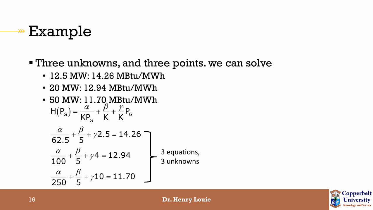
Example
Three unknowns, and three points. we can solve• 12.5 MW: 14.26 MBtu/MWh
• 20 MW: 12.94 MBtu/MWh
• 50 MW: 11.70 MBtu/MWh
Dr. Henry Louie16
G G
G
H P PKP K K
2.5 14.2662.5 5
4 12.94100 5
10 11.70250 5
3 equations,3 unknowns
Example
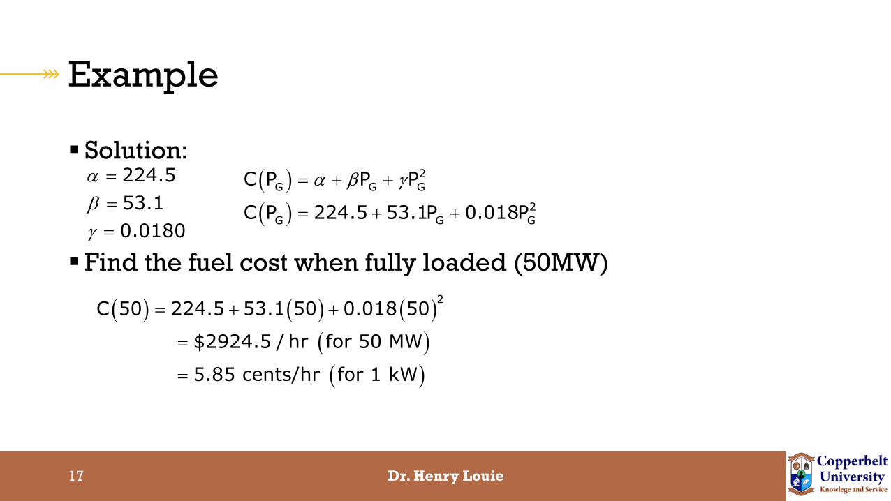
Solution:
Find the fuel cost when fully loaded (50MW)
Dr. Henry Louie17
224.5
53.1
0.0180
2
G G G
2
G G G
C P P P
C P 224.5 53.1P 0.018P
2C 50 224.5 53.1 50 0.018 50
$2924.5 / hr for 50 MW
5.85 cents/hr for 1 kW

Example
Find the fuel cost at 40% loaded, 25% loaded
Dr. Henry Louie18
224.5
53.1
0.0180

Example
Find the fuel cost at 40% loaded, 25% loaded
Dr. Henry Louie19
2
2
C 20 224.5 53.1 20 0.018 20
$1293.7 / hr for 20 MW
6.47 cents/kWh
C 12.5 224.5 53.1 12.5 0.018 12.5
$891.1 / hr for 12.5 MW
7.13 cents/kWh
224.5
53.1
0.0180

20
General Problem Formulation
Now that we have discussed how costs are computed we can formulate the general economic dispatch problem
We want to minimize the total cost while observing all the power flow equations, constraints on generators, line flow and voltage magnitude by selecting generator real power and voltage magnitudes
Dr. Henry Louie

General Problem Formulation Minimize total cost CT ($/hr)
m generators committed (on-line)
n buses
SDi given
Dr. Henry Louie21
m
T i Gii 1
min C C (P )P
min max
Gi Gi Gi
min max
i i i
max
ij Gi
P P P i 1,2, ,m
i 1,2, ,m, ,n
P P
V V V
all lines
power flow equations satisfied
subject to:
Optimization Problem

General Problem Formulation
See text page 404 for further comments (to be provided)
Economic dispatch problem is a nonlinear optimization problem
Nonlinear programming is beyond the scope of this class
We will make some problem alterations
Dr. Henry Louie22

Assumptions
Losses ignored
Weak dependence on voltage magnitude and reactive power demand
Therefore, we expect the voltage magnitudes and reactive power demand to have little effect on the flow of real power
We then make the approximation that all voltages are equal to 1.0 p.u. and formulate the problem entirely based on real power generation and flows
Dr. Henry Louie23

24
Classical Economic Dispatch
Tmin C ( )P
P
m n
Gi D Dii 1 i 1
P P P
min max
Gi Gi GiP P P i 1,2, ,m
subject to
conservation of power
if we ignore generator limits the problem becomes very simple
Dr. Henry Louie
Simplified ED Problem

Classical Economic Dispatch
Incremental costs (IC)
Derivative of fuel cost curve
What are the units?• dollars/MWh
Linear, monotonically increasing
Dr. Henry Louie25
i Gi
i
Gi
i i i Gi
dC PIC
dP
IC 2 P

Optimal Dispatch Rule Consider two generators
operating at different incremental costs to serve a 150 MW load
If we decrease PG1 by 10 MW, we decrease the cost by a significant amount (large slope)
PG2 increases by 10, but the cost only mildly increases (small slope)
Dr. Henry Louie26
PG1 (MW)
C1
(PG
1)
PG2 (MW)
C2
(PG
2)
100
50
slope = IC1
slope = IC2

27
Optimal Dispatch Rule
Using the problem as formulated on the previous slide, if we have no losses and no generator limits then:
Operating the generator at the same incremental cost is the optimal solution
• note 1: this rule only gives an optimality condition, not a solution (but the problem has been greatly reduced)
• note 2: it is implicitly assumed that there are no constraints preventing the generators from operating at the same incremental cost
Dr. Henry Louie
28
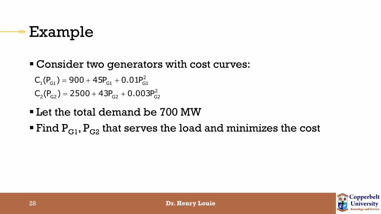
Example
Consider two generators with cost curves:
Let the total demand be 700 MW
Find PG1, PG2 that serves the load and minimizes the cost
2
1 G1 G1 G1
2
2 G2 G2 G2
C (P ) 900 45P 0.01P
C (P ) 2500 43P 0.003P
Dr. Henry Louie

29
Example
Find the incremental cost curves:
2
1 G1 G1 G1
2
2 G2 G2 G2
C P 900 45P 0.01P
C P 2500 43P 0.003P
Dr. Henry Louie

30
Example
Find the incremental cost curves:
add the power balance constraint
2
1 G1 G1 G1
2
2 G2 G2 G2
C P 900 45P 0.01P
C P 2500 43P 0.003P
11 G1
G1
22 G2
G2
dCIC 45 0.02P
dP
dCIC 43 0.006P
dP
G1 G2
P P 700
Dr. Henry Louie

31
Example
We have three equations, and three unknowns; solve
11 G1
G1
22 G2
G2
G1 G2
dCIC 45 0.02P
dP
dCIC 43 0.006P
dP
P P 700
G1 G2
G1 G2
G1
G2
45 0.02P 43 0.006P
P 700 P
P 84.6MW
P 615.4MW
Dr. Henry Louie
32
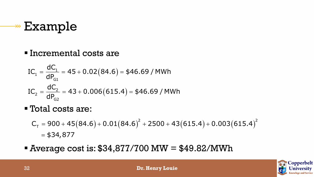
Example
Incremental costs are
Total costs are:
Average cost is: $34,877/700 MW = $49.82/MWh
11
G1
22
G2
dCIC 45 0.02 84.6 $46.69 / MWh
dP
dCIC 43 0.006 615.4 $46.69 / MWh
dP
2 2
TC 900 45 84.6 0.01 84.6 2500 43 615.4 0.003 615.4
$34,877
Dr. Henry Louie
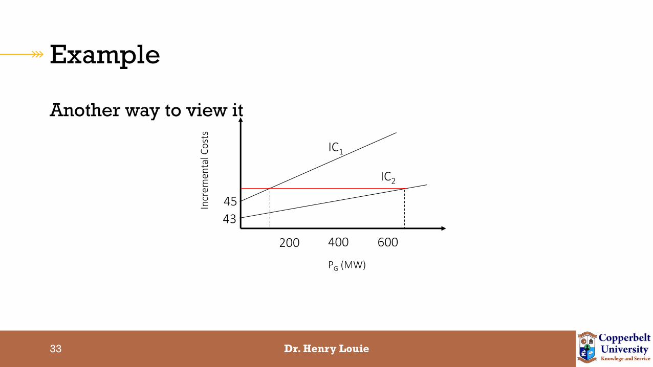
33
Example
Another way to view it
PG (MW)
Incr
emen
tal C
ost
s
200
IC1
400 600
43
45
IC2
Dr. Henry Louie

34
Optimal Dispatch Rule Proof
Using the simplified formulation we need to find the values of PGi that minimize
We have m-1 independent variables
The problem is now unconstrained
T 1 G1 2 G2 m Gm
C C (P ) C (P ) C (P )
G1 G2 Gm D
Gm D G1 G2 Gm 1
P P P P
P P P P P
T 1 G1 2 G2 m D G1 G2 Gm 1C C P C P C P P P P
Dr. Henry Louie
35
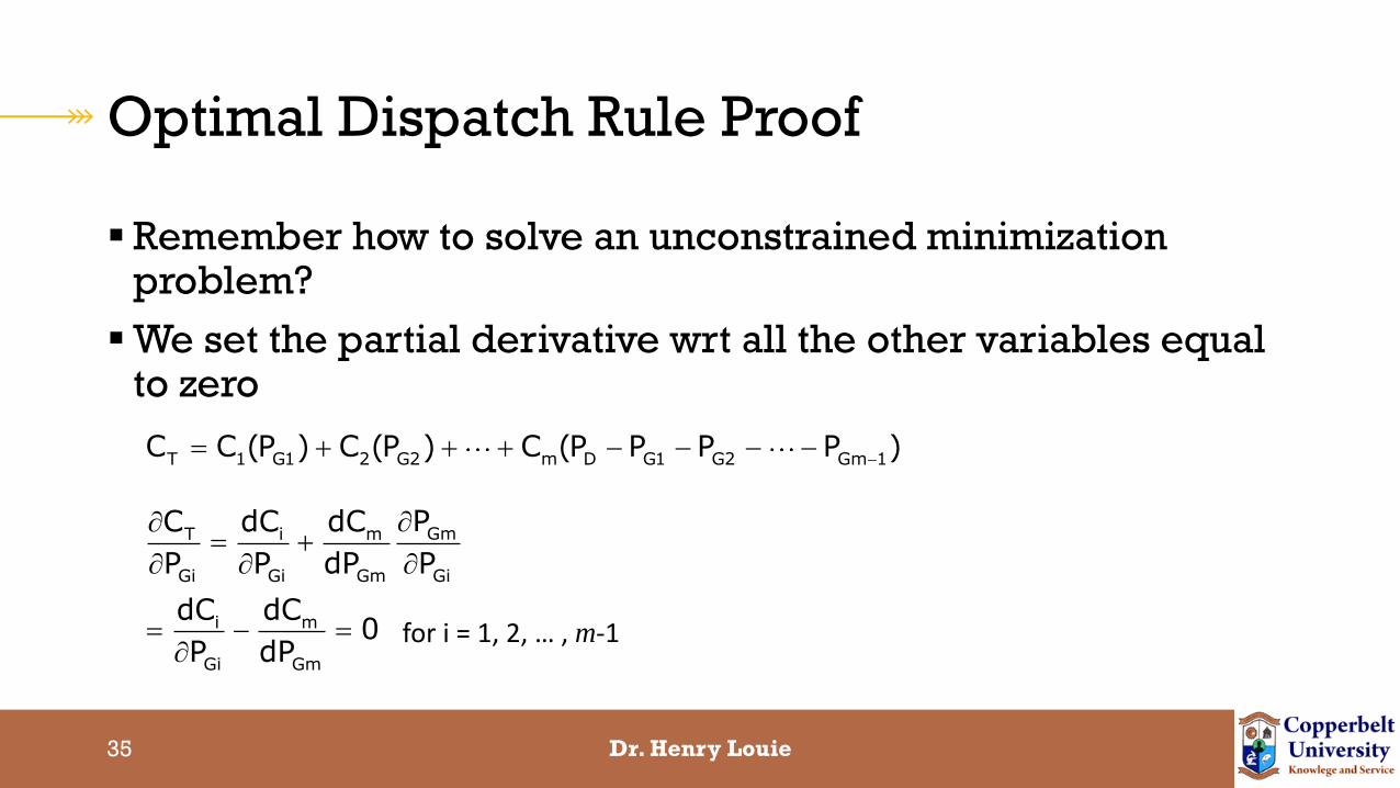
Optimal Dispatch Rule Proof
Remember how to solve an unconstrained minimization problem?
We set the partial derivative wrt all the other variables equal to zero
T 1 G1 2 G2 m D G1 G2 Gm 1C C (P ) C (P ) C (P P P P )
GmT i m
Gi Gi Gm Gi
i m
Gi Gm
PC dC dC
P P dP P
dC dC0
P dPfor i = 1, 2, … , m-1
Dr. Henry Louie

36
Optimal Dispatch Rule Proof
Note that we have assumed convexity
Assuming that the cost curves are monotonically increasing, we expect only one solution to this problem
Therefore, equal ICs is a necessary and sufficient condition to determine for optimality
Dr. Henry Louie
37
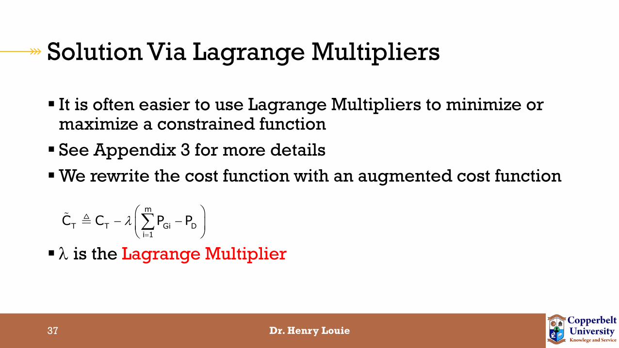
Solution Via Lagrange Multipliers
It is often easier to use Lagrange Multipliers to minimize or maximize a constrained function
See Appendix 3 for more details
We rewrite the cost function with an augmented cost function
l is the Lagrange Multiplier
l
m
T T Gi Di 1
C C P P
Dr. Henry Louie

38
Solution Via Lagrange Multipliers
Optimal point: stationary points of CT wrt l and all the PGi
variables
note: this point satisfies the constraintl
T
Gi
T
C0 i 1,2, ,m
P
C0
l
m
T T Gi Di 1
C C P P
Dr. Henry Louie

39
Solution Via Lagrange Multipliers
applied to our problem
l is the system incremental cost
l
T
Gi
m
Gi Di 1
dC i 1,2, ,m
dP
P P 0
l
m
T T G Gi Di 1
C C P PP
Dr. Henry Louie

40
Solution Via Lagrange Multipliers
Incr
emen
tal C
ost
s
IC1 IC2
l
PG1 PG2 PG3
IC3
Dr. Henry Louie

41
Solution Via Lagrange Multipliers
If the cost curves are quadratic then the incremental cost curves are linear and the problem can be readily solved
If the cost curves are nonlinear, then an iterative process is used
1) pick an initial value of l
2) find the corresponding PG1(l), PG2(l), PG3(l)
3) if the generation is less than load, then increase l and repeat step 2. if the generation is greater than the load, decrease l and repeat step 2. If generation and load balance then stop.
Dr. Henry Louie

42
Generator Limits Included
Formulation so far as ignored generator constraints, we now will add them
Tmin CP
P
m n
Gi D Dii 1 i 1
min max
Gi Gi Gi
P P P
P P P i 1,2, ,m
subject to
conservation of power
Dr. Henry Louie
43
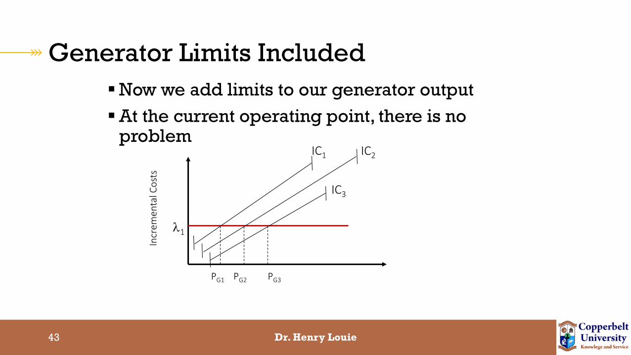
Generator Limits Included
Now we add limits to our generator output
At the current operating point, there is no problem
Incr
emen
tal C
ost
s IC1 IC2
l1
PG1 PG2 PG3
IC3
Dr. Henry Louie

Generator Limits Included
What if the system load increases?
Dr. Henry Louie44
Incr
emen
tal C
ost
s IC1 IC2
PG1 PG2 PG3
IC3
l1
l2

45
Generator Limits Included What if the system load increases further?
Operate Gen 3 at PG3, gen 1 and gen 2 should have equal l
Incr
emen
tal C
ost
s IC1 IC2
l1
PG1 PG2 PG3
IC3l2
l3
Dr. Henry Louie

46
Optimal Dispatch Rule (No losses)
Operate all generators that are not at their limits at equal l
Procedure: pick a l such that all generators operate at the same incremental costs and within their constraints
If the generation is not equal to the load at this l, then adjust las in the unconstrained case
Repeat this process until the load is met, or a generator reaches is limit
If a generator reaches its limit, then fix its output to the limit and continue to adjust the other values
Dr. Henry Louie

47
Optimal Dispatch Rule (No losses)
Note 1: it usually helpful to draw graphs of the incremental curves
Note 2: this rule applies to committed generators only (already on-line)
Note 3: this rule can be interpreted as trying to operate the system as closely as possible to equal incremental costs
Dr. Henry Louie

48
Example
Assume there are two generators with cost functions:
Let the generator limits be:
if PD = 700, find the optimal dispatch
2
1 G1 G1 G1
2
2 G2 G2 G2
C P 900 45P 0.01P
C P 2500 43P 0.003P
G1
G2
50MW P 200MW
50MW P 600MW
Dr. Henry Louie

49
Example
Start with an initial l guess• l = 45.5
Is this feasible? • No (PG1 <50MW)
Is the demand met?• No, so increase l• We don’t fix PG1 at its minimum since we need to increase l
1 G1 G1
2 G2 G2
IC 45.5 45 0.02P P 25
IC 45.5 43 0.006P P 416.7
2
1 G1 G1 G1
2
2 G2 G2 G2
C P 900 45P 0.01P
C P 2500 43P 0.003P
Dr. Henry Louie
50
Example
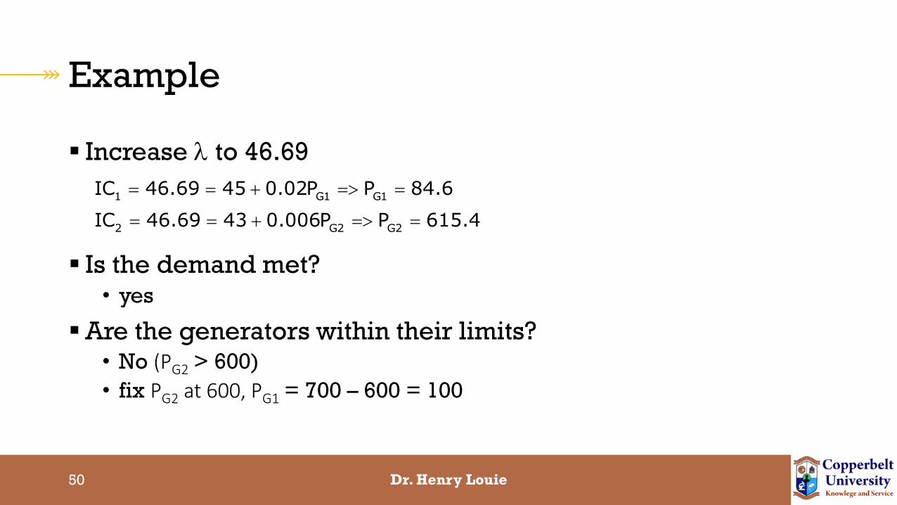
Increase l to 46.69
Is the demand met?• yes
Are the generators within their limits? • No (PG2 > 600)
• fix PG2 at 600, PG1 = 700 – 600 = 100
1 G1 G1
2 G2 G2
IC 46.69 45 0.02P P 84.6
IC 46.69 43 0.006P P 615.4
Dr. Henry Louie

51
Example
PG (MW)
Incr
emen
tal C
ost
s
200
IC1
400 600
46.69IC2
Dr. Henry Louie

52
Line Losses Considered
Line losses can reasonably be neglected if all the generators are located geographically close to one another
However, this may not be the case. we then need to account for transmission loses
Generators closer to the loads will tend to have lower losses than those far away
Dr. Henry Louie
53
Line Losses Considered
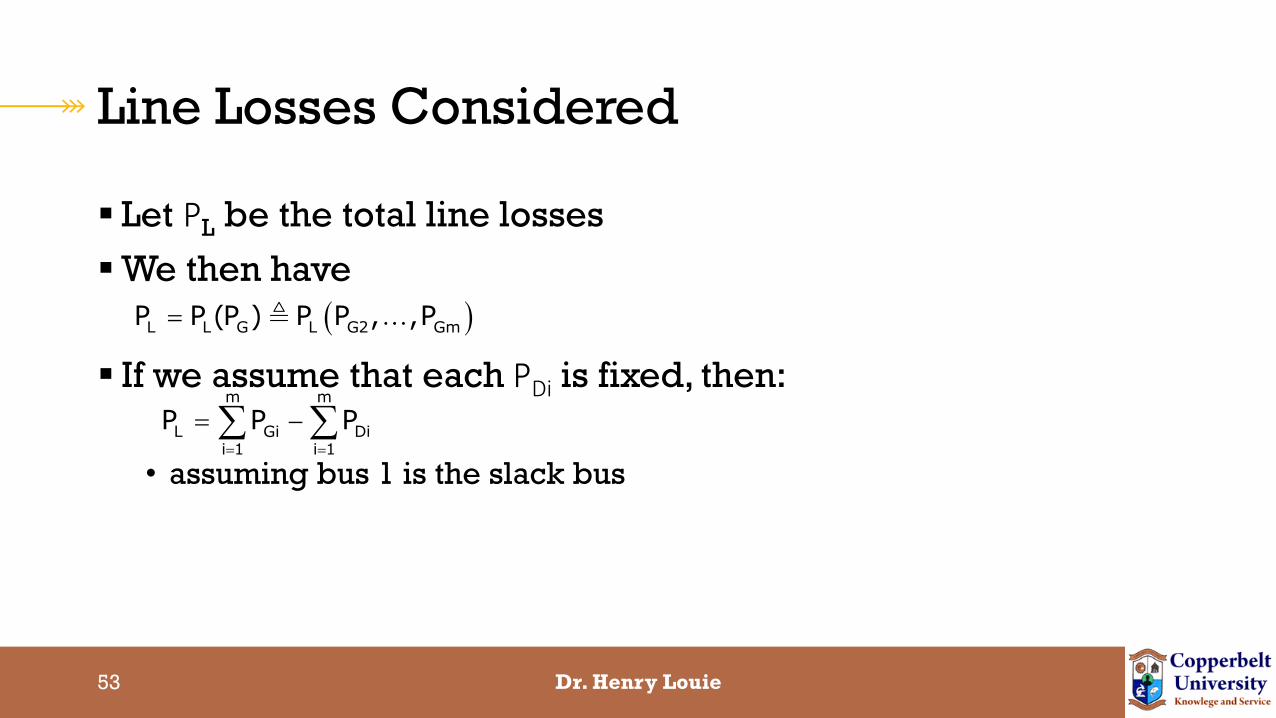
Let PL be the total line losses
We then have
If we assume that each PDi is fixed, then:
• assuming bus 1 is the slack bus
m m
L Gi Dii 1 i 1
P P P
L L G L G2 Gm
P P (P ) P P , ,P
Dr. Henry Louie

54
Line Losses Considered
G
T Gmin CP
P
m n
Gi L G2 Gm Dii 1 i 1
min max
Gi Gi Gi
P P P , ,P P 0
P P P i 1,2, ,m
subject to
Dr. Henry Louie

55
Line Losses Considered
Once again, we will use Lagrange multipliers (for now, ignore generator limits)
The stationary points are:
l
m m n
T i Gi Gi L G2 Gm Dii 1 i 1 i 1
C C P P P P , ,P P 0
l
l
l
m
TGi L D
i 1
T 1
G1 G1
T i L
Gi Gi Gi
dCP P P 0
d
dC dC0 (slack bus)
dP dP
dC dC P1 0 i 2,...,m
dP dP P
Dr. Henry Louie

56
Line Losses Considered
rewrite
as
now define:
T i L
Gi Gi Gi
dC dC P1 0 i 2,...,m
dP dP Pl
i
L Gi
Gi
dC1 i 2,...,m
P dP1
P
l
1
iL
Gi
L 1
1L i 2,...,m
P1
P
Dr. Henry Louie
57
Line Losses Considered
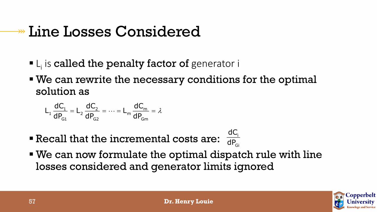
Li is called the penalty factor of generator i
We can rewrite the necessary conditions for the optimal solution as
Recall that the incremental costs are:
We can now formulate the optimal dispatch rule with line losses considered and generator limits ignored
1 2 m1 2 m
G1 G2 Gm
dC dC dCL L L
dP dP dPl
i
Gi
dC
dP
Dr. Henry Louie

58
Optimal Dispatch Rule (Line Losses Considered, No Generator Limit)
Operate all generators so that Li x ICi = l for every generator
Note: we no longer need to operate each generator at the same incremental cost
Dr. Henry Louie

59
Optimal Dispatch Rule (Line Losses Considered)
Operate all generators not at their limits so that Li x ICi = l
Dr. Henry Louie