02/06/2008CSCI 315 Operating Systems Design1 CPU Scheduling Algorithms Notice: The slides for this lecture have been largely based on those accompanying

02/06/2008 CSCI 315 Operating Systems Design 1

CPU Scheduling Algorithms

Notice: The slides for this lecture have been largely based on those accompanying the textbook Operating Systems Concepts with Java, by Silberschatz, Galvin, and Gagne (2007). Many, if not all, the illustrations contained in this presentation come from this source.


Basic Concepts• You want to maximize CPU utilization through

the use of multiprogramming.

• Each process repeatedly goes through cycles that alternate CPU execution (a CPU burst) and I/O wait (an I/O wait).

• Empirical evidence indicates that CPU-burst lengths have a distribution such that there is a large number of short bursts and a small number of long bursts.


Preemptive Scheduling

• In cooperative or nonpreemptive scheduling, when a process takes the CPU, it keeps it until the process either enters waiting state or terminates.

• In preemptive scheduling, a process holding the CPU may lose it. Preemption causes context-switches, which introduce overhead. Preemption also calls for care when a process that loses the CPU is accessing data shared with another process or kernel data structures.


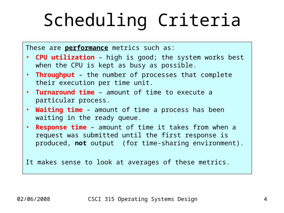
Scheduling Criteria

These are performance metrics such as:

• CPU utilization – high is good; the system works best when the CPU is kept as busy as possible.

• Throughput – the number of processes that complete their execution per time unit.

• Turnaround time – amount of time to execute a particular process.

• Waiting time – amount of time a process has been waiting in the ready queue.

• Response time – amount of time it takes from when a request was submitted until the first response is produced, not output (for time-sharing environment).

It makes sense to look at averages of these metrics.


Scheduling AlgorithmsScheduling Algorithms


First-Come, First-Served (FCFS)

Process Burst Time

P1 24

P2 3

P3 3

• Suppose that the processes arrive in the order: P1 , P2 , P3

The Gantt Chart for the schedule is:

• Waiting time for P1 = 0; P2 = 24; P3 = 27• Average waiting time: (0 + 24 + 27)/3 = 17

P1 P2 P3

24 27 300


FCFS

Suppose that the processes arrive in the order

P2 , P3 , P1

• The Gantt chart for the schedule is:

• Waiting time for P1 = 6; P2 = 0; P3 = 3

• Average waiting time: (6 + 0 + 3)/3 = 3• Much better than previous case.• Convoy effect: all process are stuck waiting until a long process terminates.

P1P3P2

63 300


Shortest-Job-First (SJF)• Associate with each process the length of its next CPU

burst. Use these lengths to schedule the process with the shortest time.

• Two schemes: – Nonpreemptive – once CPU given to the process it cannot be

preempted until completes its CPU burst.– Preemptive – if a new process arrives with CPU burst length

less than remaining time of current executing process, preempt. This scheme is know as the Shortest-Remaining-Time-First (SRTF).

• SJF is optimal – gives minimum average waiting time for a given set of processes.

Question: Is this practical? How can one determine the length of a CPU-burst?


Process Arrival Time Burst Time

P1 0.0 7

P2 2.0 4

P3 4.0 1

P4 5.0 4

• SJF (non-preemptive)

• Average waiting time = (0 + 6 + 3 + 7)/4 = 4

Non-Preemptive SJF

P1 P3 P2

73 160

P4

8 12


Preemptive SJF

Process Arrival Time Burst Time

P1 0.0 7

P2 2.0 4

P3 4.0 1

P4 5.0 4

• SJF (preemptive)

• Average waiting time = (9 + 1 + 0 +2)/4 = 3

P1 P3P2

42 110

P4

5 7

P2 P1

16


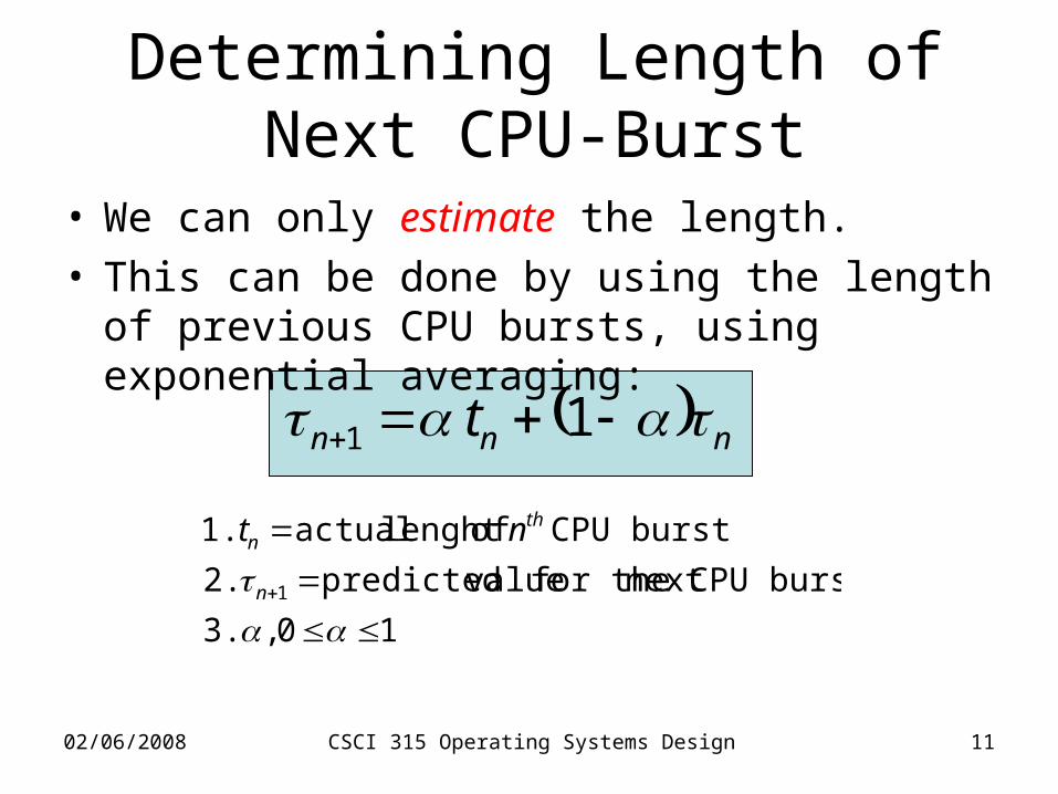
Determining Length of Next CPU-Burst

• We can only estimate the length.• This can be done by using the length of previous

CPU bursts, using exponential averaging:

10 , 3.

burst CPUnext for the valuepredicted 2.

burst CPU oflenght actual 1.

1

n

thn nt

nnn t 1 1


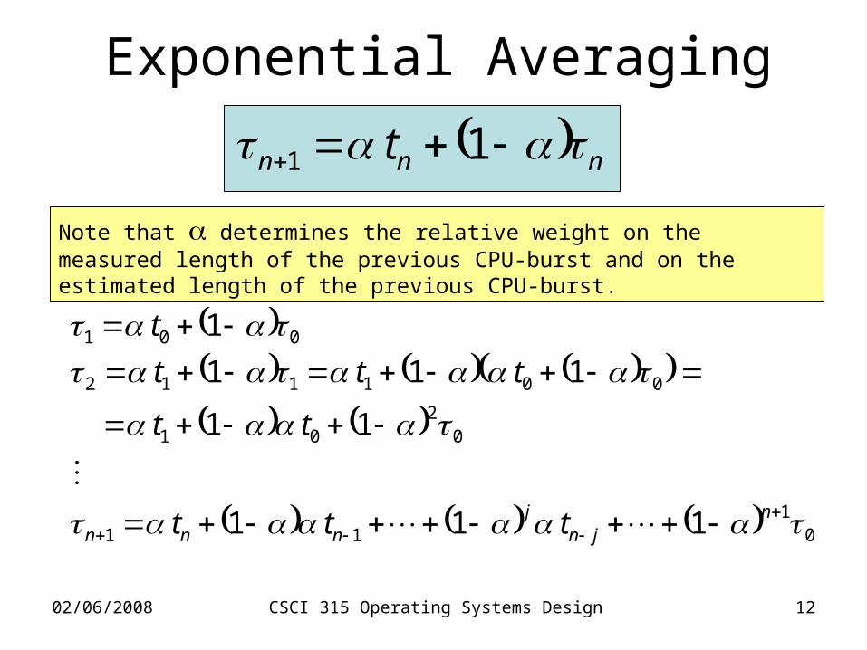
Exponential Averaging

nnn t 1 1

01

11

02

01

001112

001

1 1 1

1 1

1 1 1

1

njn

jnnn ttt

tt

ttt

t

Note that determines the relative weight on the measured length of the previous CPU-burst and on the estimated length of the previous CPU-burst.


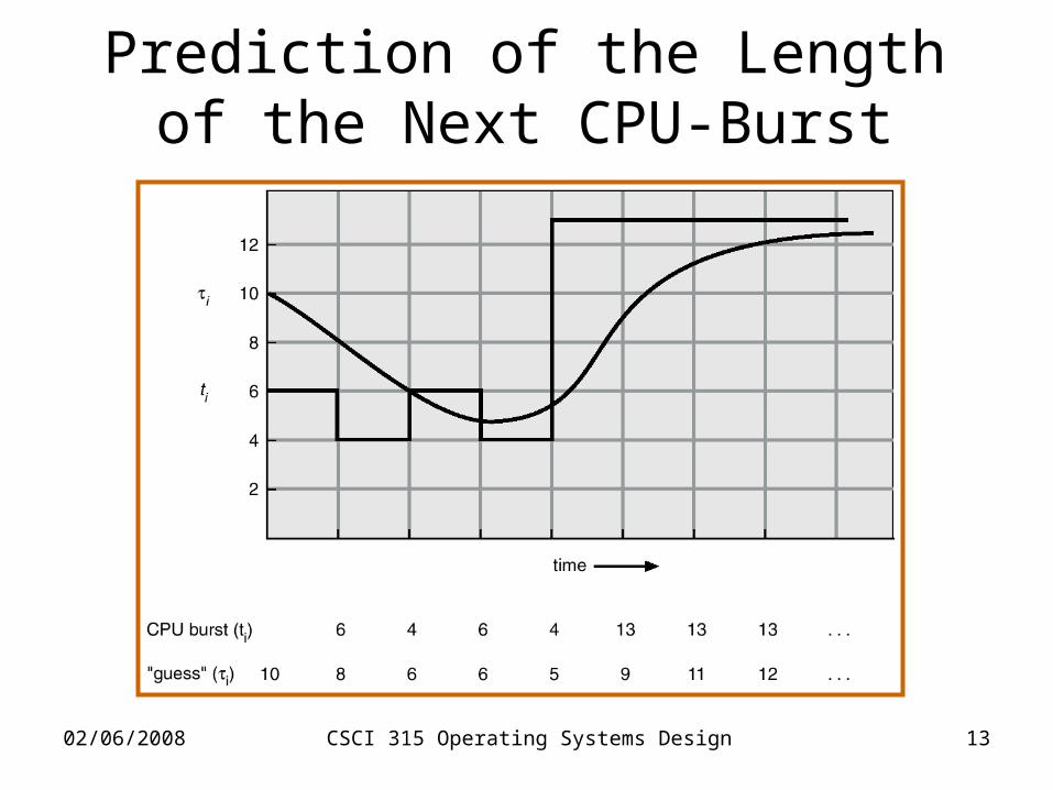
Prediction of the Length of the Next CPU-Burst


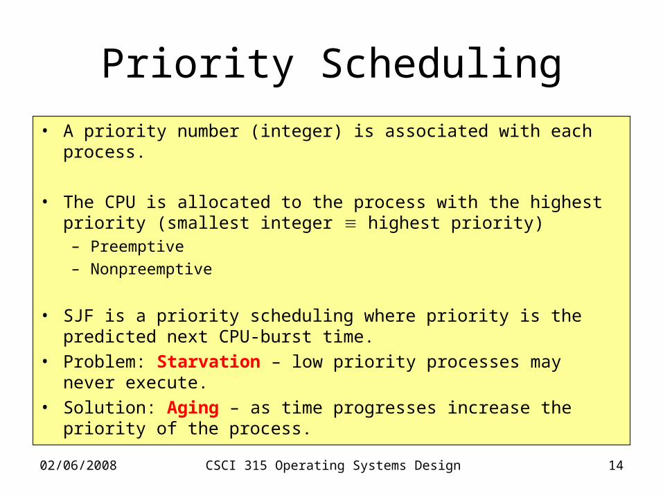
Priority Scheduling

• A priority number (integer) is associated with each process.

• The CPU is allocated to the process with the highest priority (smallest integer highest priority)– Preemptive

– Nonpreemptive

• SJF is a priority scheduling where priority is the predicted next CPU-burst time.

• Problem: Starvation – low priority processes may never execute.• Solution: Aging – as time progresses increase the priority of the

process.


Round Robin (RR)• Each process gets a small unit of CPU time (time quantum), usually 10-100 milliseconds. After this time has elapsed, the process is preempted and added to the end of the ready queue.

• If there are n processes in the ready queue and the time quantum is q, then each process gets 1/n of the CPU time in chunks of at most q time units at once. No process waits more than (n-1)q time units.

• Performance:– q large FIFO.– q small q must be large with respect to context switch,

otherwise overhead is too high.


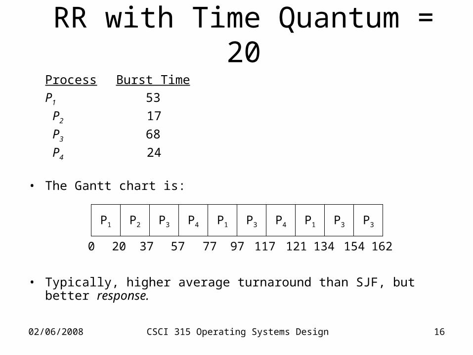
RR with Time Quantum = 20Process Burst Time

P1 53

P2 17

P3 68

P4 24

• The Gantt chart is:

• Typically, higher average turnaround than SJF, but better response.

P1 P2 P3 P4 P1 P3 P4 P1 P3 P3

0 20 37 57 77 97 117 121 134 154 162


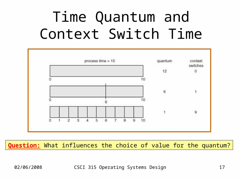
Time Quantum and Context Switch Time

Question: What influences the choice of value for the quantum?


Turnaround Time Varies with the Time Quantum


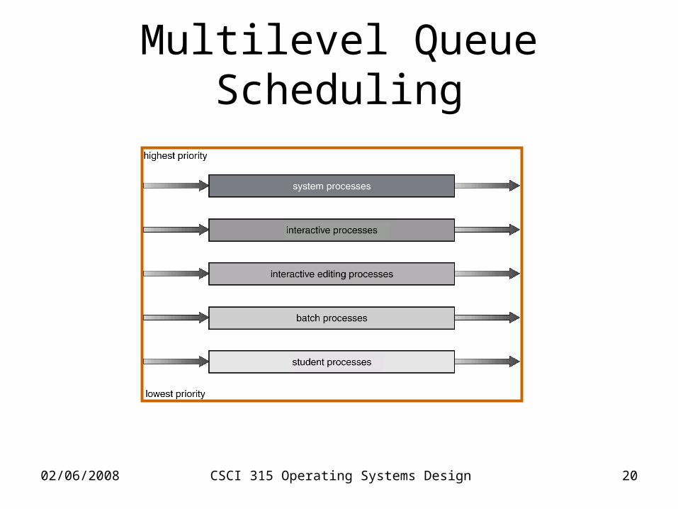
Multilevel Queue• Ready queue is partitioned into separate queues:

– foreground (interactive)

– background (batch)

• Each queue has its own scheduling algorithm.– foreground: RR

– background: FCFS

• Scheduling must be done between the queues:– Fixed priority scheduling; (i.e., serve all from foreground then from

background). Possibility of starvation.

– Time slice – each queue gets a certain amount of CPU time which it can schedule amongst its processes; i.e., 80% to foreground in RR.

– 20% to background in FCFS .


Multilevel Queue Scheduling


Multilevel Feedback Queue

• A process can move between the various queues; aging can be implemented this way.

• Multilevel-feedback-queue scheduler defined by the following parameters:– number of queues,– scheduling algorithms for each queue,– method used to determine when to upgrade a process,– method used to determine when to demote a process,– method used to determine which queue a process will enter

when that process needs service.


Example of Multilevel Feedback Queue

• Three queues: – Q0 – time quantum 8 milliseconds

– Q1 – time quantum 16 milliseconds

– Q2 – FCFS

• Scheduling– A new job enters queue Q0 which is served FCFS. When it gains

CPU, job receives 8 milliseconds. If it does not finish in 8 milliseconds, job is moved to queue Q1.

– At Q1 job is again served FCFS and receives 16 additional milliseconds. If it still does not complete, it is preempted and moved to queue Q2.


Multilevel Feedback Queues

Documents

02/06/2008CSCI 315 Operating Systems Design1 CPU Scheduling Algorithms Notice: The slides for this lecture have been largely based on those accompanying