Biostatistics for biomedical professionBIMM18

Karin Källén & Linda Hartman

September 2016

20

16

-09

-02

1

Statistics: Populations and samples

Population

Sample

Probability

Inferential statistics

Descriptivestatistics 2

01

6-0

9-0

2

2

Statistics

• Descriptive statistics

Methods to summarize (the variablesin) a sample

• Summary measures

• Graphical methods

• Inferential statistics

Methods to learn about the population that the sample is drawnfrom

• Effect measures (w confidence intervals)

• Tests (ttest chi2-test Mann-Whitney …)

20

16

-09

-02

3

Today:Basic• numerical

summaries of data• graphical

summaries of data

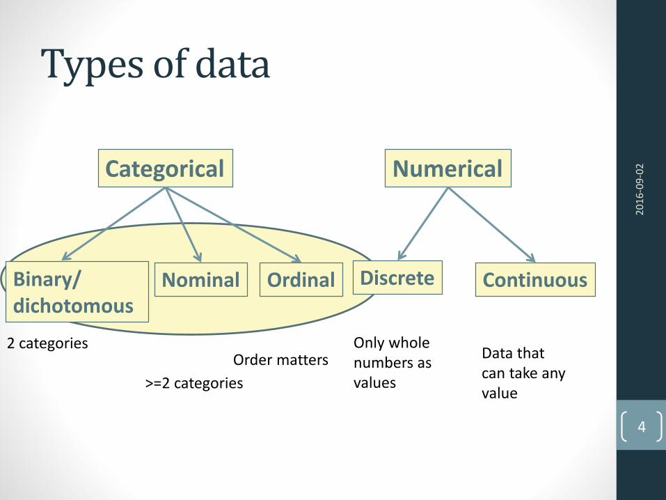
Types of data

Categorical Numerical

Binary/dichotomous

Nominal Discrete ContinuousOrdinal

2 categories

>=2 categories

Order mattersOnly wholenumbers as values

Data thatcan take anyvalue

20

16

-09

-02

4

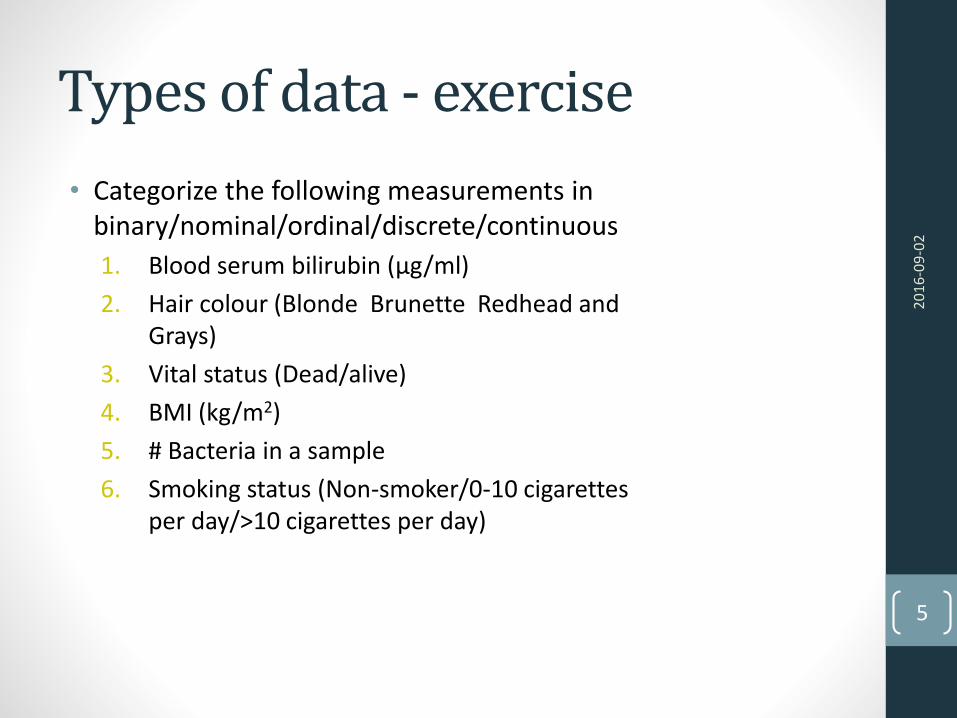
Types of data - exercise

• Categorize the following measurements in binary/nominal/ordinal/discrete/continuous

1. Blood serum bilirubin (μg/ml)

2. Hair colour (Blonde Brunette Redhead and Grays)

3. Vital status (Dead/alive)

4. BMI (kg/m2)

5. # Bacteria in a sample

6. Smoking status (Non-smoker/0-10 cigarettesper day/>10 cigarettes per day)

20

16

-09

-02

5

Binary

Nominal

Continuous

Continuous

Discrete

Ordinal

Summary measures & Graphical presentationChapter 2 & 3 in Kirkwood and Sterne

20

16

-09

-02

6

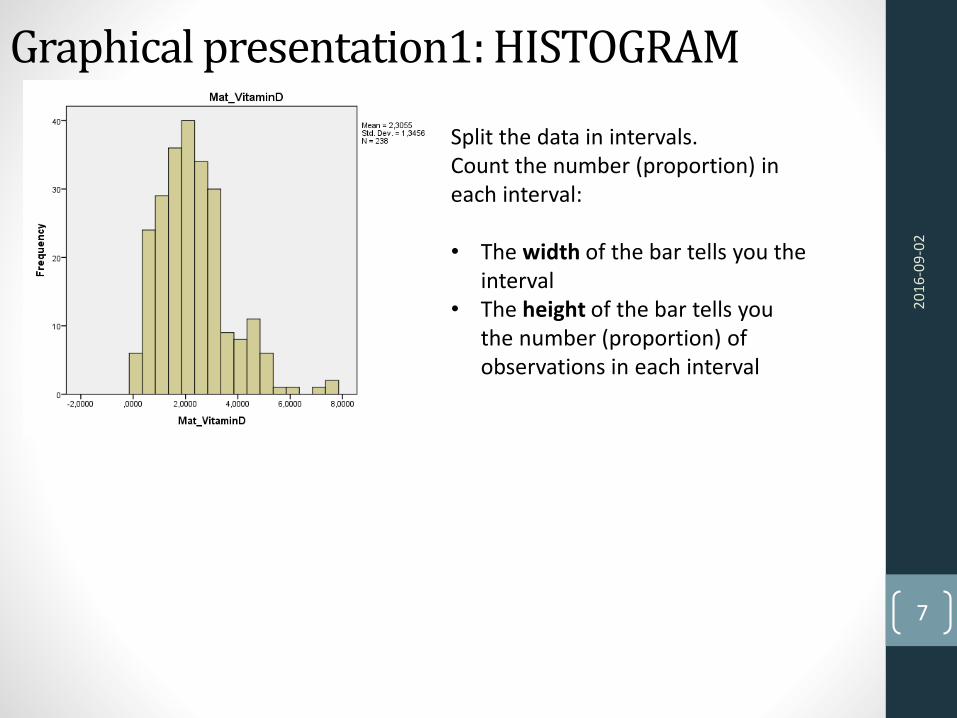
Graphical presentation1: HISTOGRAM

20

16

-09

-02

7

Split the data in intervals. Count the number (proportion) in each interval:

• The width of the bar tells you the interval

• The height of the bar tells youthe number (proportion) of observations in each interval

Summary measures:

• Average measures (“Central tendency”)

Describe a “center” around which the measurements

in the data are distributed

• Dispersion (or Variability) measures

Describe “data spread” or how far away

the measurements are from the center.

20

16

-09

-02

8

Average measuresAverage measures (“Central tendency”)Describe a “center” around which the measurementsin the data are distributed

20

16

-09

-02

9

Average measures• Median

‐ The middle observation if data are sorted

• Mean‐ The sum of the observations devided by

the number of observations

‐

• Mode‐ The most frequently occuring value

ഥ𝑿 =𝑿𝟏 + 𝑿𝟐 +⋯+ 𝑿𝑵

𝑵=𝟏

𝑵

𝒊=𝟏

𝑵

𝑿𝒊

20

16

-09

-02

10

Average measures - exercise

Exercise:

• Calculate the mean, median and mode of a dataset with the following values: 4 8 6 3 4

20

16

-09

-02

11

Mean: 25/5 = 5

Median: 4

Mode: 4

Central tendency

Mean or medianThe choice depends on thedistribution of the data:

• Symmetric data

• Asymmetric data

• Ordinal data

Symmetric distributionAsymmetric distribution

20

16

-09

-02

12

General recommendations:

Use the mean

Use the median

Use the median

Central tendency

Nominal data

Average measuresare not meaningful.

Use number of observations and proportions

20

16

-09

-02

13

Barchart

Central tendency measures Summary

Type of data Central tendencymeasure

Symmetric data Mean

Asymmetric data Median

Ordinal Median

Nominal -

20

16

-09

-02

14

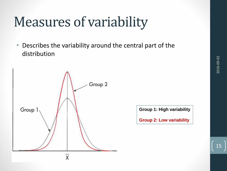
Measures of variability

• Describes the variability around the central part of the distribution

Group 1: High variability

Group 2: Low variability

20

16

-09

-02

15

Measures of dispersion

• Standard deviation – The mean deviation from the mean value

• Percentiles & quartiles

– Splits the data in fixed proportions

• Range – The difference between min and max

20

16

-09

-02

16

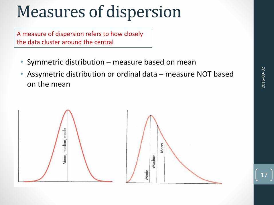
Measures of dispersion

• Symmetric distribution – measure based on mean

• Assymetric distribution or ordinal data – measure NOT basedon the mean

A measure of dispersion refers to how closelythe data cluster around the central

20

16

-09

-02

17

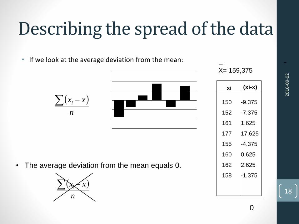
Describing the spread of the data

• If we look at the average deviation from the mean:

n

xxi

n

xxi

• The average deviation from the mean equals 0.

xi (xi-x)

150

152

161

177

155

160

162

158

-9.375

-7.375

1.625

17.625

-4.375

0.625

2.625

-1.375

0

X= 159,375

20

16

-09

-02

18

Describing the spread of the

data• If we square every term we solve the problem with 0.

n

xxi 2

1

2

n

xxi

To get a better estimate we use n-1 in the denominator

This is called the VARIANCE!

The variance is expressed in cm2 which is unpractical

since the mean length is expressed in cm

150

152

161

177

155

160

162

158

-9.375

-7.375

1.625

17.625

-4.375

0.625

2.625

-1.375

x (𝐱 − ഥ𝒙) 𝐱 − ഥ𝒙 𝟐

2

87.89

54.39

2.64

310.64

19.14

0.39

6.89

1.89

0 483.87

= 60.48

20

16

-09

-02

19

Describing the spread of the data

1

2

n

xxs

i

By taking the square root of the variance, you get the

standard deviation (standard deviation = SD) which has

the same units as what you measured

20

16

-09

-02

20

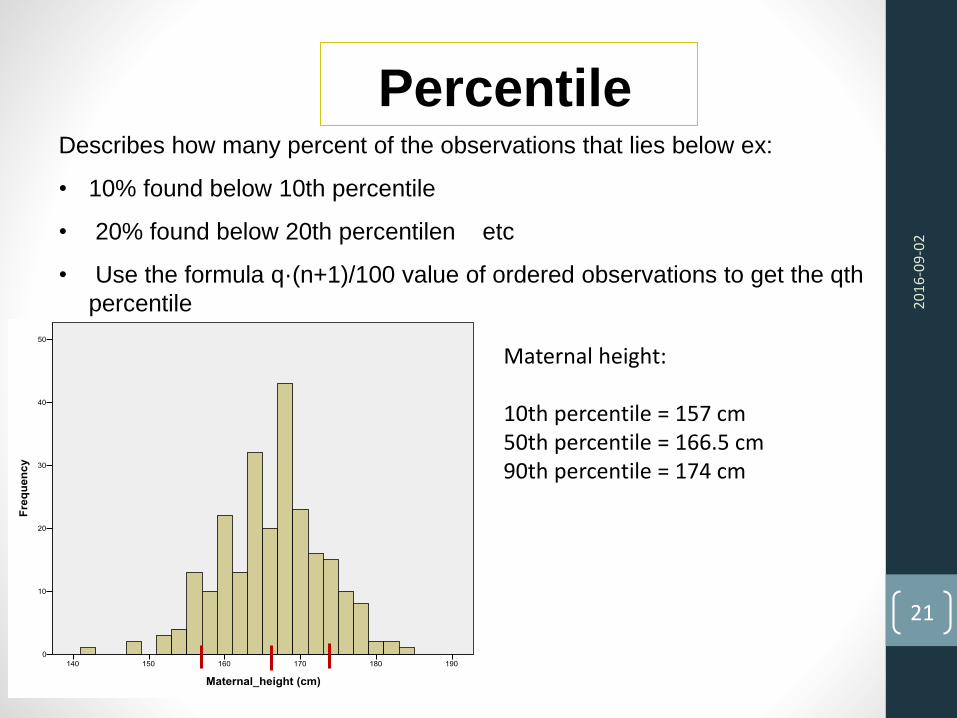
PercentileDescribes how many percent of the observations that lies below ex:

• 10% found below 10th percentile

• 20% found below 20th percentilen etc

• Use the formula q·(n+1)/100 value of ordered observations to get the qth

percentile 20

16

-09

-02

21

Maternal height:

10th percentile = 157 cm50th percentile = 166.5 cm90th percentile = 174 cm

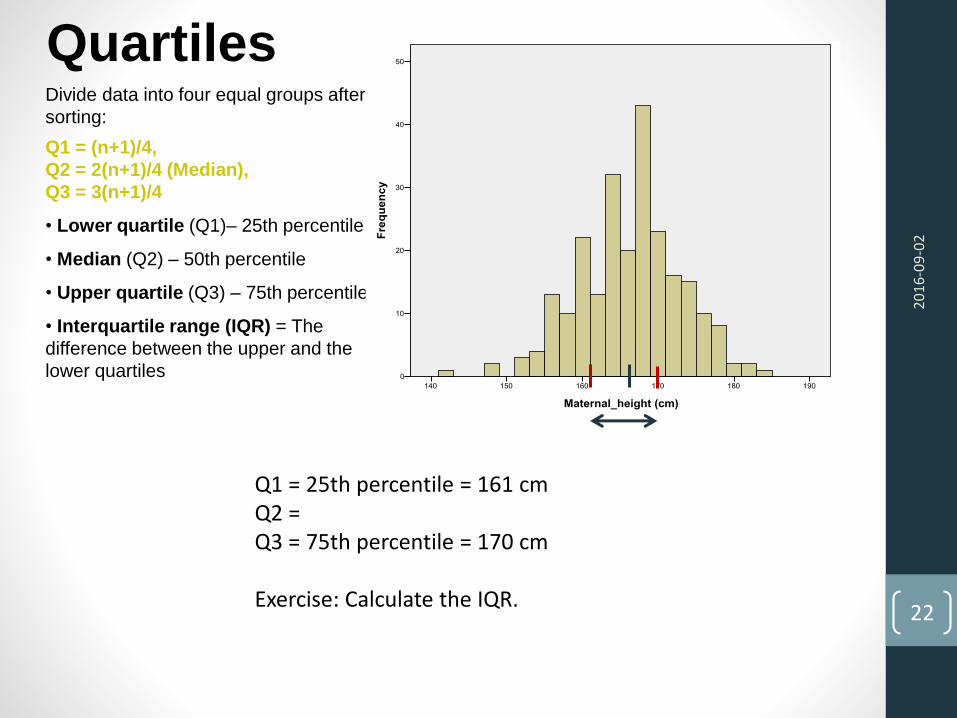
QuartilesDivide data into four equal groups after

sorting:

Q1 = (n+1)/4,

Q2 = 2(n+1)/4 (Median),

Q3 = 3(n+1)/4

• Lower quartile (Q1)– 25th percentile

• Median (Q2) – 50th percentile

• Upper quartile (Q3) – 75th percentile

• Interquartile range (IQR) = The

difference between the upper and the

lower quartiles

20

16

-09

-02

22

Q1 = 25th percentile = 161 cmQ2 = Q3 = 75th percentile = 170 cm

Exercise: Calculate the IQR.

Measures of dispersion

Exercise

• Calculate the standard deviation and rangefor a dataset with the following values: 4 8 6 3 4

20

16

-09

-02

23

Mean: 25/5 = 5

Median: 4

Mode: 4

Range: 8-3=5

S= √( 1/(5-1) ) * [(4-5)2 +(8-5)2+(6-5)2+(3-5)2+(4-5)2] =√(¼) * [1+9+1+4+1]= √4 = 2

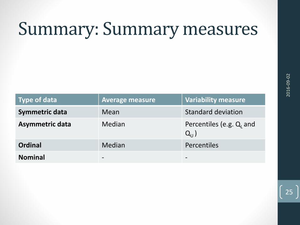
Summary: Summary measures

Type of data Average measure Variability measure

Symmetric data Mean Standard deviation

Asymmetric data Median Percentiles (e.g. QL andQU )

Ordinal Median Percentiles

Nominal - -

20

16

-09

-02

25

Graphical presentation 2: Box-plot

20

16

-09

-02

26

Max

Q3

Median

Q1

Min

BOX-PLOT

20

16

-09

-02

27

383339N =

Fiskkonsumtionsgrupp

HögMediumLåg

CB

_153 (

ng/g

lip

idvik

t)

3000

2000

1000

0

Low medium high

Fish consumption

Outlier O

Observationes more than 1.5 IQR outside the box

Extreme values *Observations more than 3 IQR outside the box

Lowest ”normal” value

Lower quartile QL

Median

Upper quartile QU

Highest ”normal” value

(Inner fence)

Inter quartile range (IQR)=QU –QL = Box-length

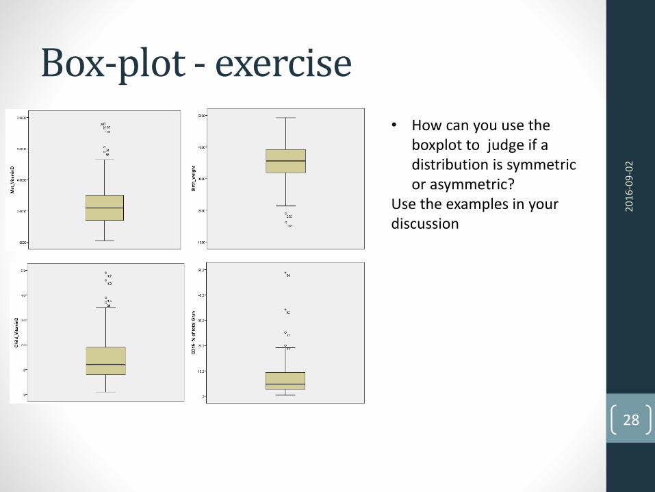
Box-plot - exercise

20

16

-09

-02

28

• How can you use the boxplot to judge if a distribution is symmetricor asymmetric?

Use the examples in yourdiscussion

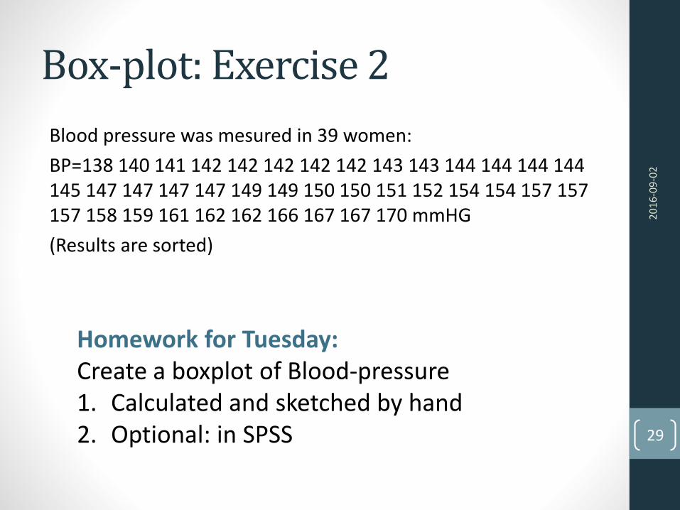
Box-plot: Exercise 2

Blood pressure was mesured in 39 women:

BP=138 140 141 142 142 142 142 142 143 143 144 144 144 144 145 147 147 147 147 149 149 150 150 151 152 154 154 157 157 157 158 159 161 162 162 166 167 167 170 mmHG

(Results are sorted)

20

16

-09

-02

29

Homework for Tuesday: Create a boxplot of Blood-pressure1. Calculated and sketched by hand2. Optional: in SPSS

20

16

-09

-02

30

Summary:‐ Types of variables (binary/nominal/ordinal/discrete/continuous)- Descriptive statistics

- Central tendency measures (mean median)- Dispersion measures (standard deviation percentiles)

- Graphical presentation- Barplot- Histogram- Boxplot

Next lecture:Subject K&S

Normal distribution 5

Population, samples, generalizability 4.5, 6.3, 8.5

Hypothesis testing, Error types p-values 8

Reference interval Confidence interval 6

T-test 7.1-7.4

ANOVA 9.1-9.2