Embed Size (px)
Citation preview
PHYS 705: Classical MechanicsHamilton-Jacobi Equation
1
Hamilton-Jacobi Equation
There is also a very elegant relation between the Hamiltonian
Formulation of Mechanics and Quantum Mechanics.
The Hamilton-Jacobi equation also represents a very general method in
solving mechanical problems.
Let say we are able to find a canonical transformation taking our 2n phase
space variables directly to 2n constants of motion, i.e., ,i iq p
To do that, we need to derive the Hamilton-Jacobi equation.
i iP i iQ
,i i
2
To start…
Hamilton-Jacobi Equation
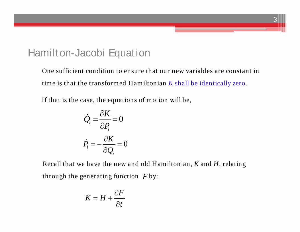
One sufficient condition to ensure that our new variables are constant in
time is that the transformed Hamiltonian K shall be identically zero.
If that is the case, the equations of motion will be,
Recall that we have the new and old Hamiltonian, K and H, relating
through the generating function by:
0ii
KQP
0ii
KPQ
F
3
FK Ht
Hamilton-Jacobi Equation
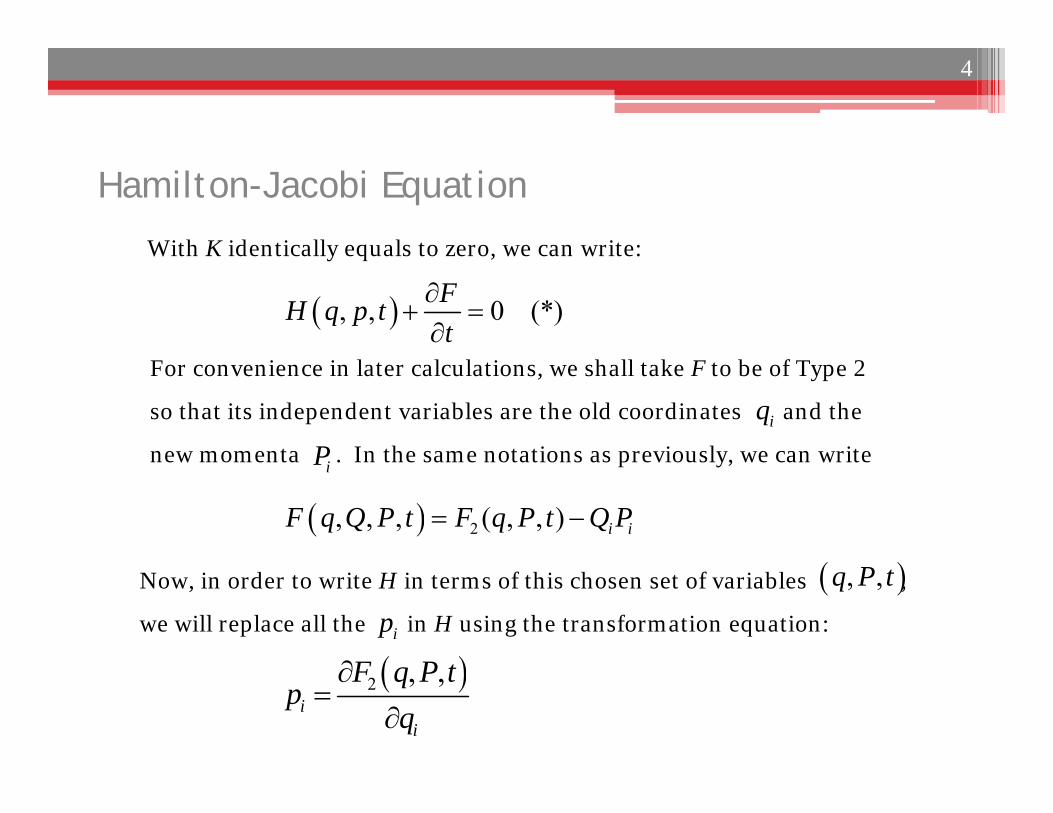
With K identically equals to zero, we can write:
For convenience in later calculations, we shall take F to be of Type 2
so that its independent variables are the old coordinates and the
new momenta . In the same notations as previously, we can write
Now, in order to write H in terms of this chosen set of variables ,
we will replace all the in H using the transformation equation:
2 , ,i
i
F q P tp
q
2, , , ( , , ) i iF q Q P t F q P t Q P
, , 0 (*)FH q p tt
iq
iP
, ,q P t
ip
4
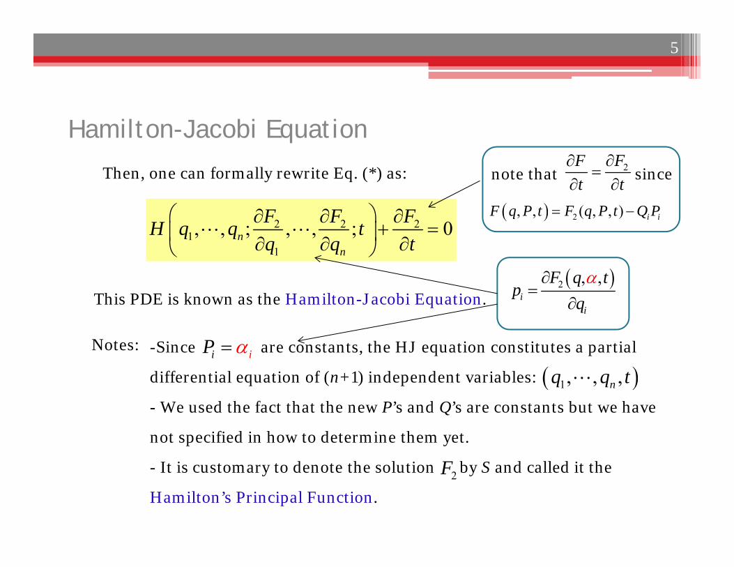
-Since are constants, the HJ equation constitutes a partial
differential equation of (n+1) independent variables:
- We used the fact that the new P’s and Q’s are constants but we have
not specified in how to determine them yet.
- It is customary to denote the solution by S and called it the
Hamilton’s Principal Function.
Hamilton-Jacobi Equation
Then, one can formally rewrite Eq. (*) as: note that since
This PDE is known as the Hamilton-Jacobi Equation.
2, , ( , , ) i iF q P t F q P t Q P 2 2 2
11
, , ; , , ; 0nn
F F FH q q tq q t
1, , ,nq q t
2FFt t
Notes:iiP
2F
5
2 , ,i
i
F q tp
q
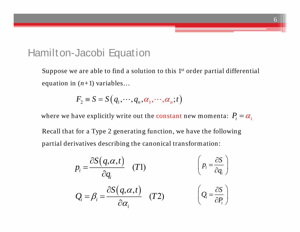
Recall that for a Type 2 generating function, we have the following
partial derivatives describing the canonical transformation:
Hamilton-Jacobi Equation
Suppose we are able to find a solution to this 1st order partial differential
equation in (n+1) variables…
where we have explicitly write out the constant new momenta:
2 1 1, , ,, , ;n nF S S q q t
iiP
, ,( 1)i
i
S q tp T
q
, ,( 2)i i
i
S q tQ T
6
ii
Spq
ii
SQP
Hamilton-Jacobi Equation
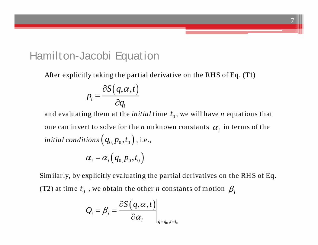
After explicitly taking the partial derivative on the RHS of Eq. (T1)
and evaluating them at the initial time , we will have n equations that
one can invert to solve for the n unknown constants in terms of the
initial conditions , i.e.,
Similarly, by explicitly evaluating the partial derivatives on the RHS of Eq.
(T2) at time , we obtain the other n constants of motion
i
, ,i
i
S q tp
q
0t
0, 0 0,i i q p t
0t i
0 0,
, ,i i
i q q t t
S q tQ
7
0, 0 0,q p t
Hamilton-Jacobi Equation
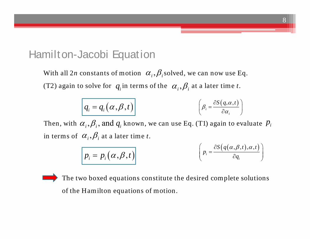
With all 2n constants of motion solved, we can now use Eq.
(T2) again to solve for in terms of the at a later time t.
The two boxed equations constitute the desired complete solutions
of the Hamilton equations of motion.
,i i
, ,i iq q t , ,i
i
S q t
,i i iq
Then, with known, we can use Eq. (T1) again to evaluate
in terms of at a later time t.
, , and i i iq ,i i
, ,i ip p t , , , ,
ii
S q t tp
q
ip
8
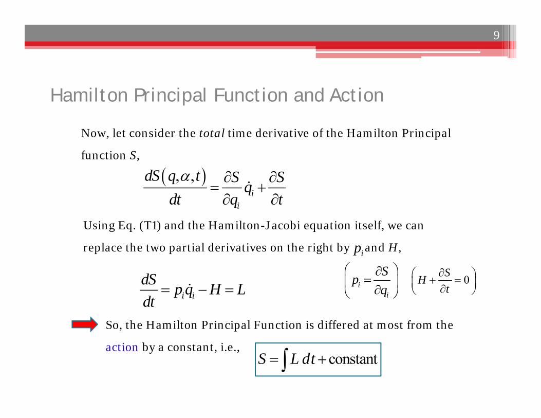
Hamilton Principal Function and Action
Now, let consider the total time derivative of the Hamilton Principal
function S,
, ,i
i
dS q t S Sqdt q t
Using Eq. (T1) and the Hamilton-Jacobi equation itself, we can
replace the two partial derivatives on the right by and H, ip
i idS p q H Ldt
ii
Spq
0SHt
So, the Hamilton Principal Function is differed at most from the
action by a constant, i.e.,constantS L dt
9
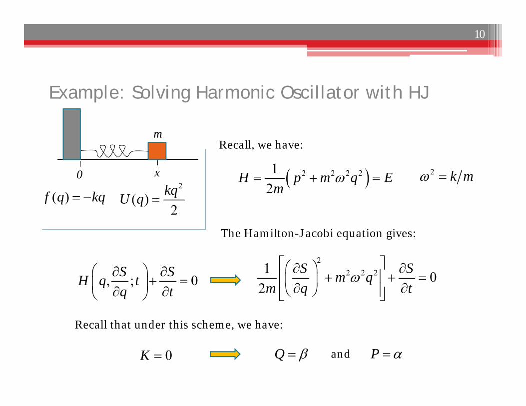
Example: Solving Harmonic Oscillator with HJ
Recall, we have:
( )f q kq
m
0 x2
( )2
kqU q
2 k m 2 2 2 212
H p m q Em
, ; 0S SH q tq t
The Hamilton-Jacobi equation gives:
22 2 21 0
2S Sm q
m q t
Recall that under this scheme, we have:
P Q 0K and
10
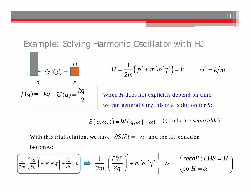
Example: Solving Harmonic Oscillator with HJ
( )f q kq
m
0 x2
( )2
kqU q
2 k m 2 2 2 212
H p m q Em
22 2 21
2W m q
m q
When H does not explicitly depend on time,
we can generally try this trial solution for S:
, , ,S q t W q t
With this trial solution, we have and the HJ equation
becomes:
S t
:sorecall LHS H
H
(q and t are separable)
11
22 2 21 0
2S Sm q
m q t
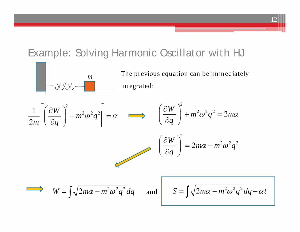
Example: Solving Harmonic Oscillator with HJ
m
22 2 2 2W m q m
q
The previous equation can be immediately
integrated:
22 2 21
2W m q
m q
22 2 22W m m q
q
2 2 22W m m q dq and 2 2 22S m m q dq t
12
1 1arcsin arcsin2mt x q
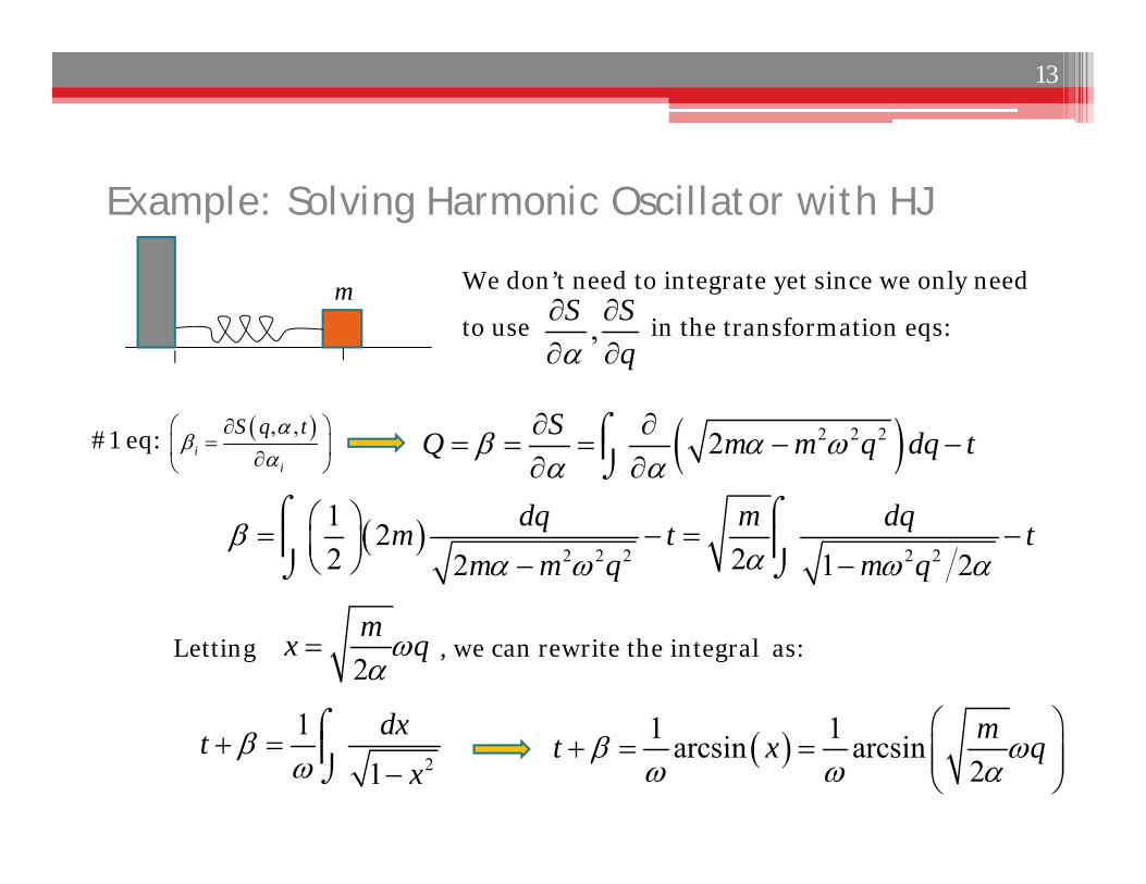
Example: Solving Harmonic Oscillator with HJ
m We don’t need to integrate yet since we only need
to use in the transformation eqs:,S Sq
2 2 22SQ m m q dq t
2 2 2 2 2
1 22 22 1 2
dq m dqm t tm m q m q
#1 eq:
2
11dxt
x
Letting , we can rewrite the integral as:2mx q
, ,i
i
S q t
13
1 1arcsin arcsin2mt x q
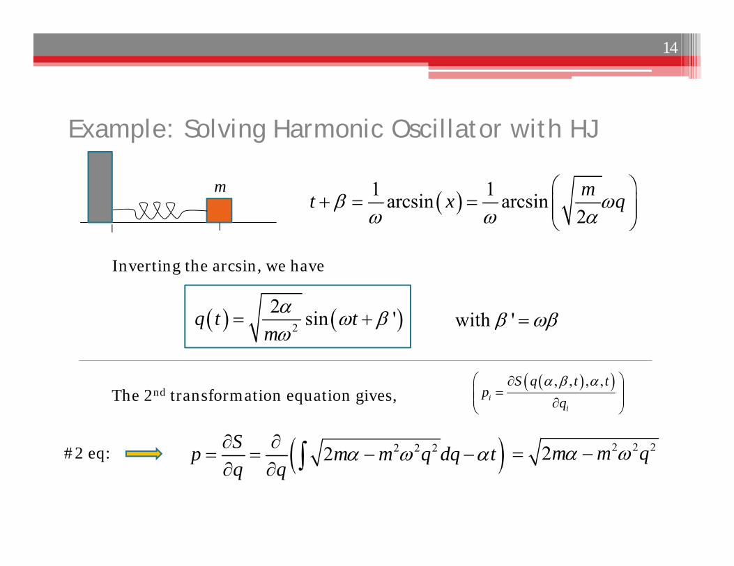
Example: Solving Harmonic Oscillator with HJ
m
Inverting the arcsin, we have
2
2 sin 'q t tm
with '
#2 eq:
The 2nd transformation equation gives,
2 2 22Sp m m q dq tq q
2 2 22m m q
, , , ,i
i
S q t tp
q
14
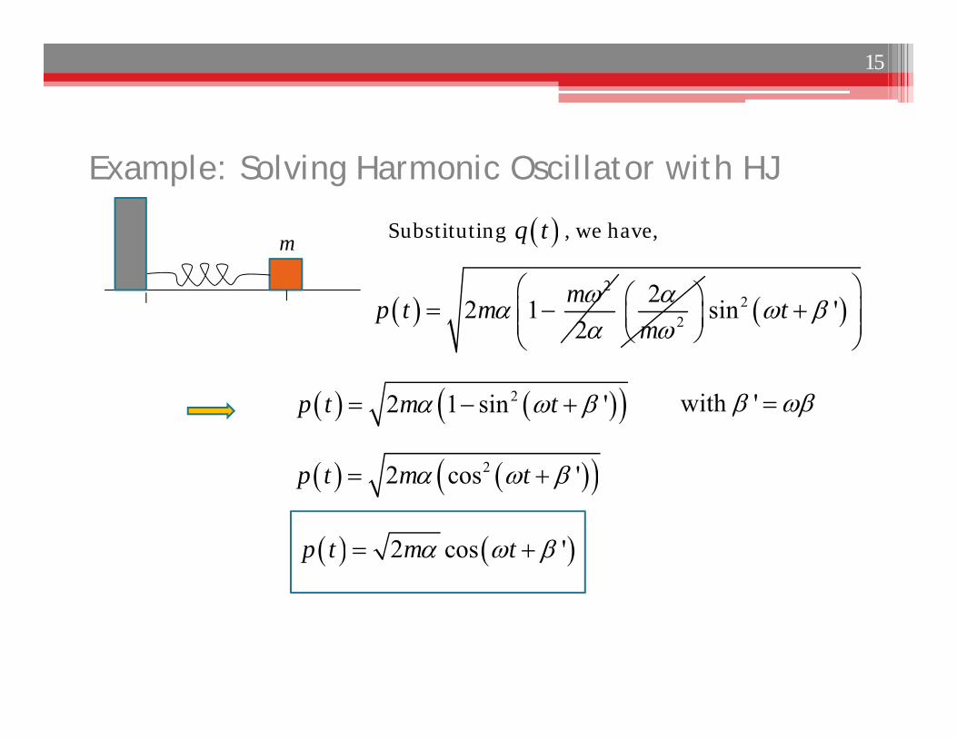
Example: Solving Harmonic Oscillator with HJ
m
with '
Substituting , we have, q t
2
2 12
mp t m
2
2m
2sin 't
22 1 sin 'p t m t
22 cos 'p t m t
2 cos 'p t m t
15
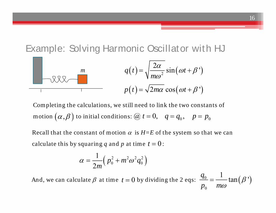
Completing the calculations, we still need to link the two constants of
motion to initial conditions:
Example: Solving Harmonic Oscillator with HJ
m
0 0@ 0, ,t q q p p
2
2 sin 'q t tm
2 cos 'p t m t
Recall that the constant of motion is H=E of the system so that we can
calculate this by squaring q and p at time :
2 2 2 20 0
12
p m qm
0t
And, we can calculate at time by dividing the 2 eqs:0t 0
0
1 tan 'qp m
16
,
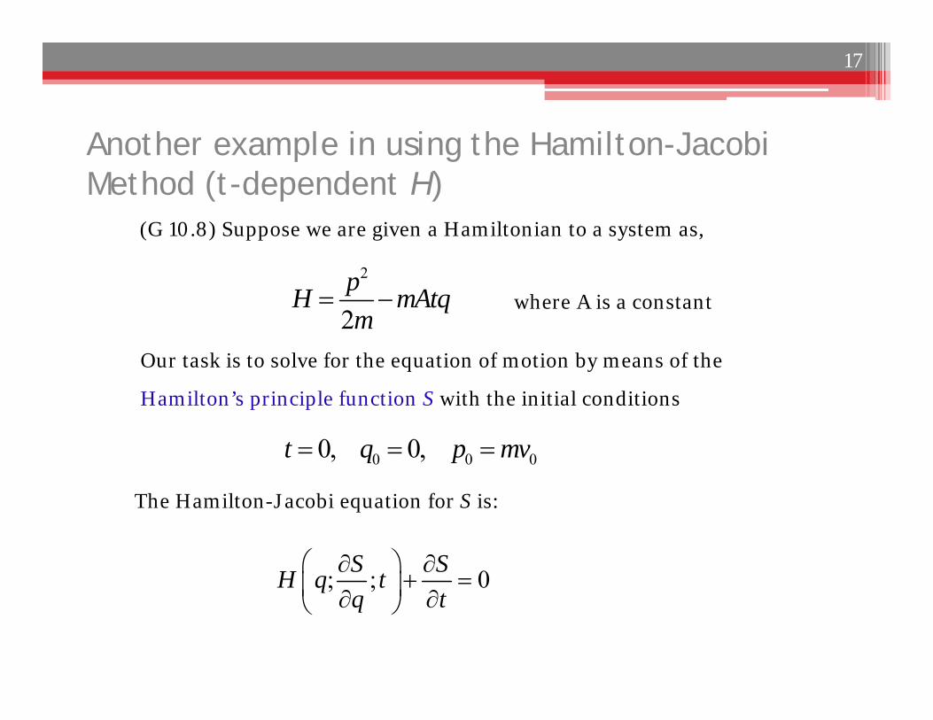
Another example in using the Hamilton-Jacobi Method (t-dependent H)
(G 10.8) Suppose we are given a Hamiltonian to a system as,
2
2pH mAtqm
where A is a constant
0 0 00, 0,t q p mv
Our task is to solve for the equation of motion by means of the
Hamilton’s principle function S with the initial conditions
The Hamilton-Jacobi equation for S is:
; ; 0S SH q tq t
17
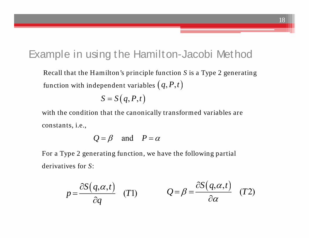
For a Type 2 generating function, we have the following partial
derivatives for S:
Example in using the Hamilton-Jacobi Method
Recall that the Hamilton’s principle function S is a Type 2 generating
function with independent variables
with the condition that the canonically transformed variables are
constants, i.e.,
, ,S S q P t
andQ P
, ,( 1)
S q tp T
q
, ,( 2)
S q tQ T
, ,q P t
18
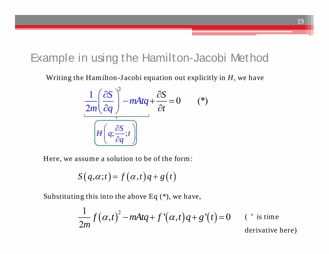
Example in using the Hamilton-Jacobi Method
Writing the Hamilton-Jacobi equation out explicitly in H, we have
Here, we assume a solution to be of the form:
2
0 (*2
)1 S mAtqm tq
S
; ;SH q tq
, ; ,S q t f t q g t
Substituting this into the above Eq (*), we have,
21 , ' , ' 02
f t mAtq f t q g tm
( is time
derivative here)
'
19
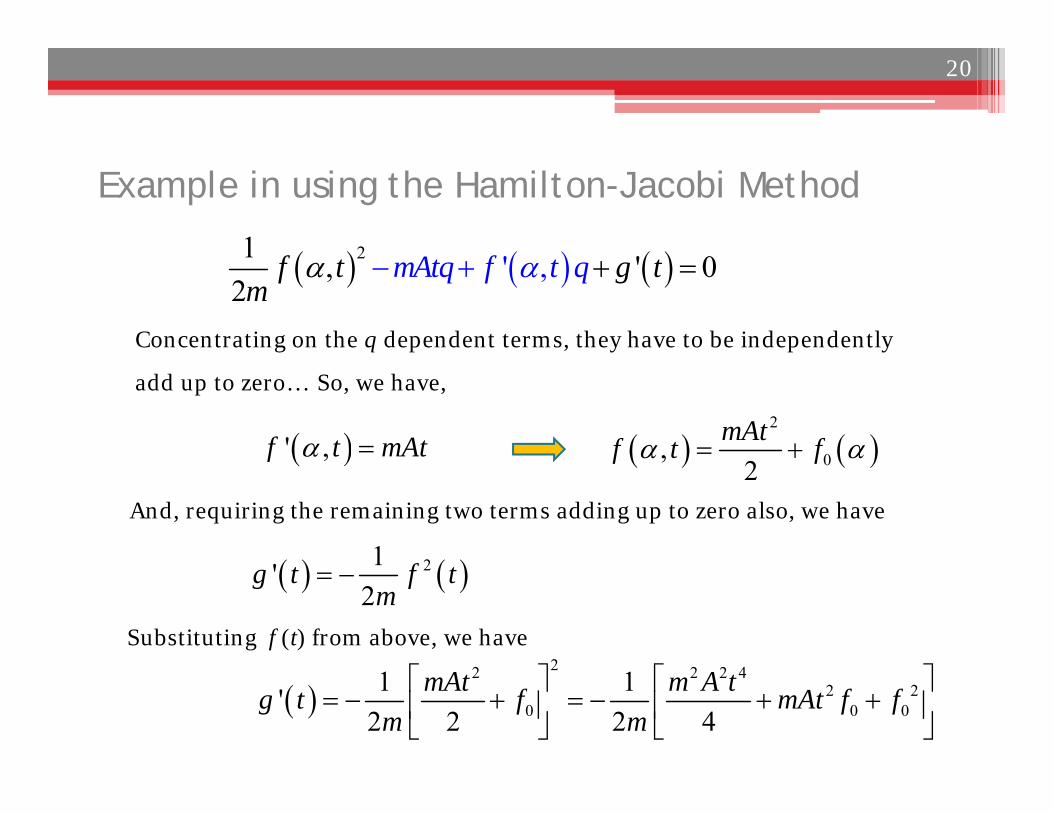
Example in using the Hamilton-Jacobi Method
Concentrating on the q dependent terms, they have to be independently
add up to zero… So, we have,
And, requiring the remaining two terms adding up to zero also, we have
' ,f t mAt
21 , 0,2
' 'mAtf tm
q f g tt q
2
0,2
mAtf t f
21'2
g t f tm
22 2 2 4
2 20 0 0
1 1'2 2 2 4
mAt m A tg t f mAt f fm m
Substituting f (t) from above, we have
20
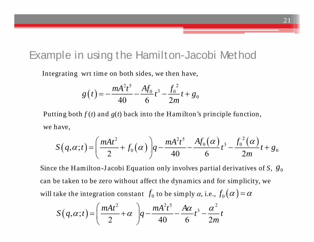
Example in using the Hamilton-Jacobi MethodIntegrating wrt time on both sides, we then have,
22 5
30 0040 6 2
Af fmA tg t t t gm
Since the Hamilton-Jacobi Equation only involves partial derivatives of S,
can be taken to be zero without affect the dynamics and for simplicity, we
will take the integration constant to be simply , i.e.,
Putting both f (t) and g(t) back into the Hamilton’s principle function,
we have,
22 2 50 03
0 0, ;2 40 6 2
Af fmAt mA tS q t f q t t gm
0g
0f 0f
2 2 5 2
3, ;2 40 6 2
mAt mA t AS q t q t tm
21
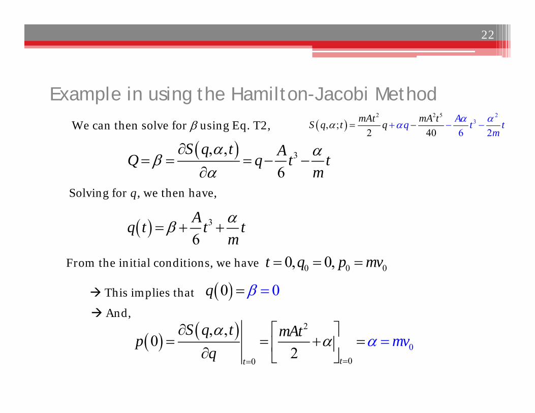
Example in using the Hamilton-Jacobi MethodWe can then solve for using Eq. T2,
From the initial conditions, we have
Solving for q, we then have,
32 5 22
6, ;
40 22mAt mA Aq t t
mtS q t q
3, ,6
S q t AQ q t tm
3
6Aq t t t
m
0 0 00, 0,t q p mv
This implies that 00q And,
2
00
0
, ,0
2 tt
S q t mAtp mvq
22
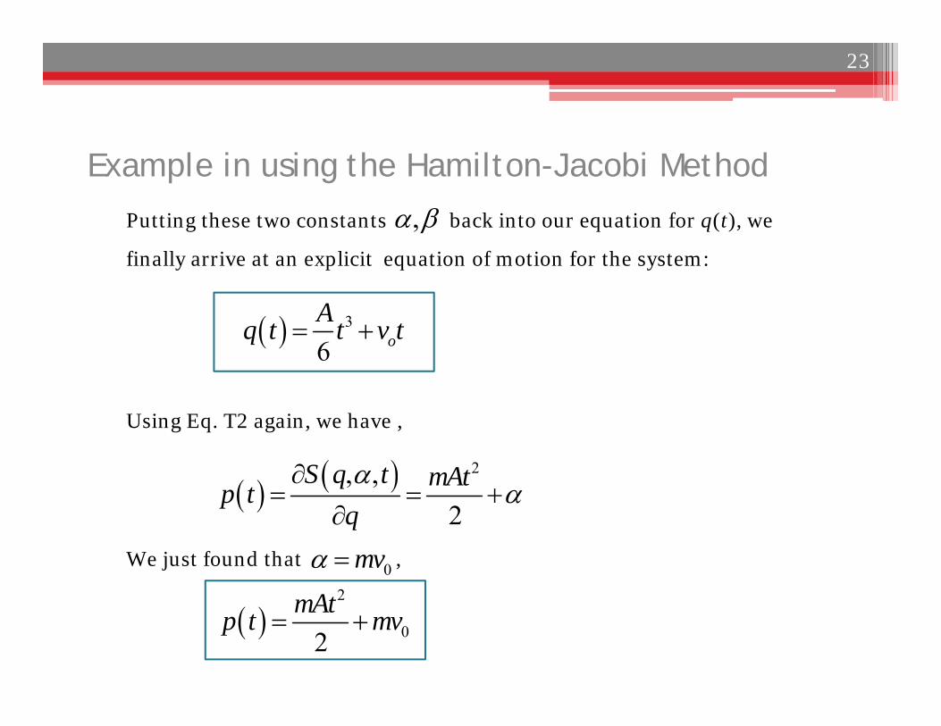
Example in using the Hamilton-Jacobi MethodPutting these two constants back into our equation for q(t), we
finally arrive at an explicit equation of motion for the system:
3
6 oAq t t v t
,
23
2, ,2
S q t mAtp tq
Using Eq. T2 again, we have ,
2
02mAtp t mv
We just found that ,0mv
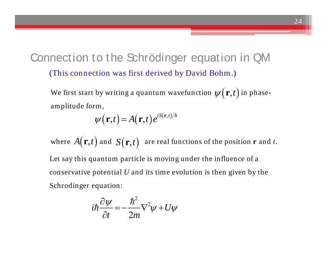
Connection to the Schrödinger equation in QM(This connection was first derived by David Bohm.)
where and are real functions of the position r and t.
Let say this quantum particle is moving under the influence of a
conservative potential U and its time evolution is then given by the
Schrodinger equation:
We first start by writing a quantum wavefunction in phase-
amplitude form,
,, , iS tt A t e rr r
,A tr ,S tr
,t r
22
2i U
t m
24

Connection to the Schrödinger equation in QMNow, we substitute the polar form of the wavefuntion into the
Schrodinger equation term by term:
:it
iS Ai e it t
1
SAt
2 : iS ie A A S
2 iS iSi i ie S A A S e A A S
2
2 2 22
22
2
1
2
iS iS
iS
i i ie S A A S e A A S A S
ie A S A SAA S
,, , iS tt A t e rr r
ImRecolor code:
ImRecolor code:
25
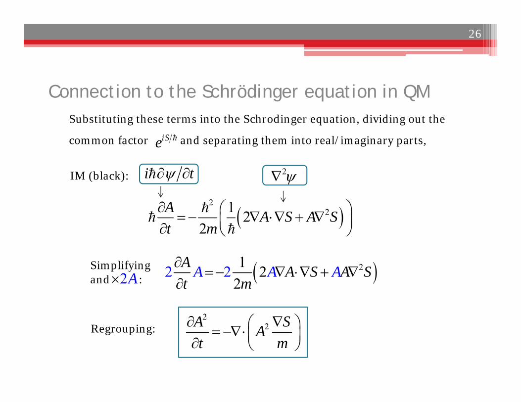
Connection to the Schrödinger equation in QM
IM (black): i t 2
21 222
2A A S A St m
A A A
Simplifying and :
Regrouping:
2
21 22
A A S A St m
2A
22A SA
t m
Substituting these terms into the Schrodinger equation, dividing out the
common factor and separating them into real/imaginary parts, iSe
26
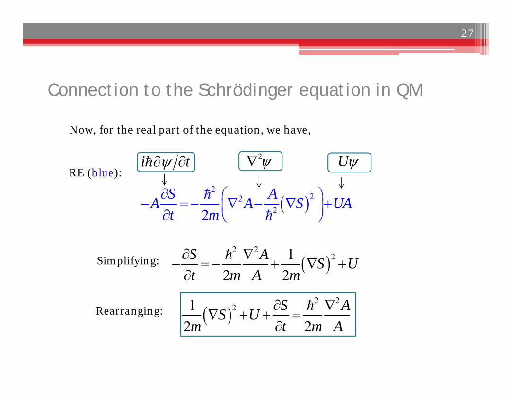
Connection to the Schrödinger equation in QM
2
2222
S AA A S UAt m
RE (blue):i t 2
2 2
212 2
S A S Ut m A m
2 2
212 2
S AS Um t m A
Simplifying:
Rearranging:
Now, for the real part of the equation, we have,
27
U
Connection to the Schrödinger equation in QM
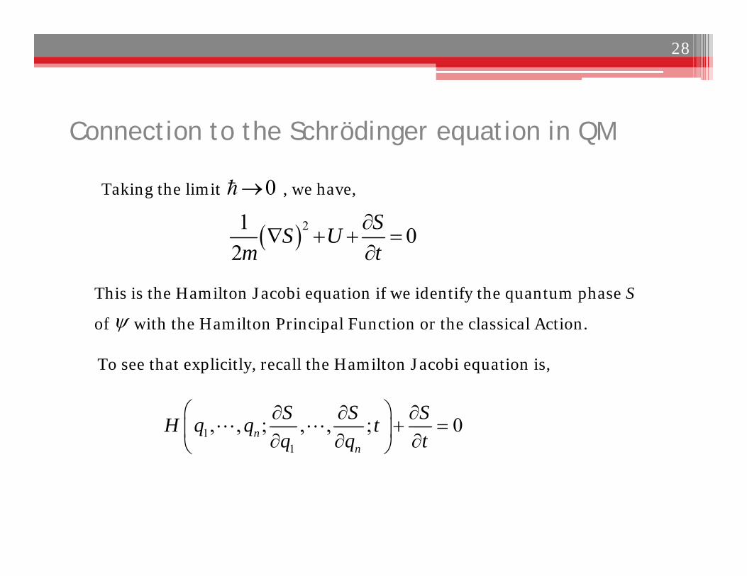
21 02
SS Um t
Taking the limit , we have,
This is the Hamilton Jacobi equation if we identify the quantum phase S
of with the Hamilton Principal Function or the classical Action.
To see that explicitly, recall the Hamilton Jacobi equation is,
11
, , ; , , ; 0nn
S S SH q q tq q t
0
28
Connection to the Schrödinger equation in QM
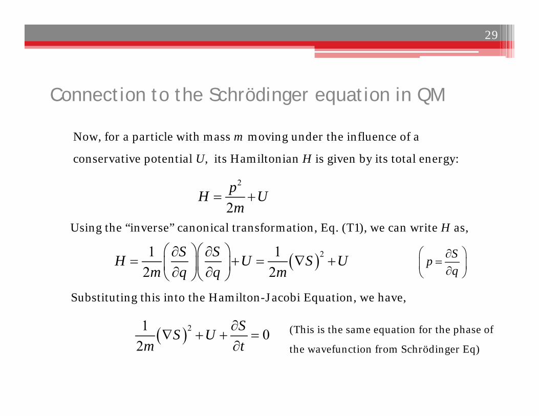
Now, for a particle with mass m moving under the influence of a
conservative potential U, its Hamiltonian H is given by its total energy:
21 12 2
S SH U S Um q q m
Using the “inverse” canonical transformation, Eq. (T1), we can write H as,
21 02
SS Um t
2
2pH Um
Substituting this into the Hamilton-Jacobi Equation, we have,
(This is the same equation for the phase of
the wavefunction from Schrödinger Eq)
Spq
29
Connection to the Schrödinger equation in QM
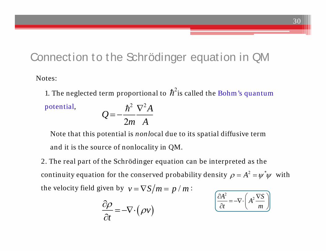
1. The neglected term proportional to is called the Bohm’s quantum
potential,
2. The real part of the Schrödinger equation can be interpreted as the
continuity equation for the conserved probability density with
the velocity field given by :
2 *A
2 2
2AQ
m A
2
vt
/v S m p m
Notes:
Note that this potential is nonlocal due to its spatial diffusive term
and it is the source of nonlocality in QM.
22A SA
t m
30
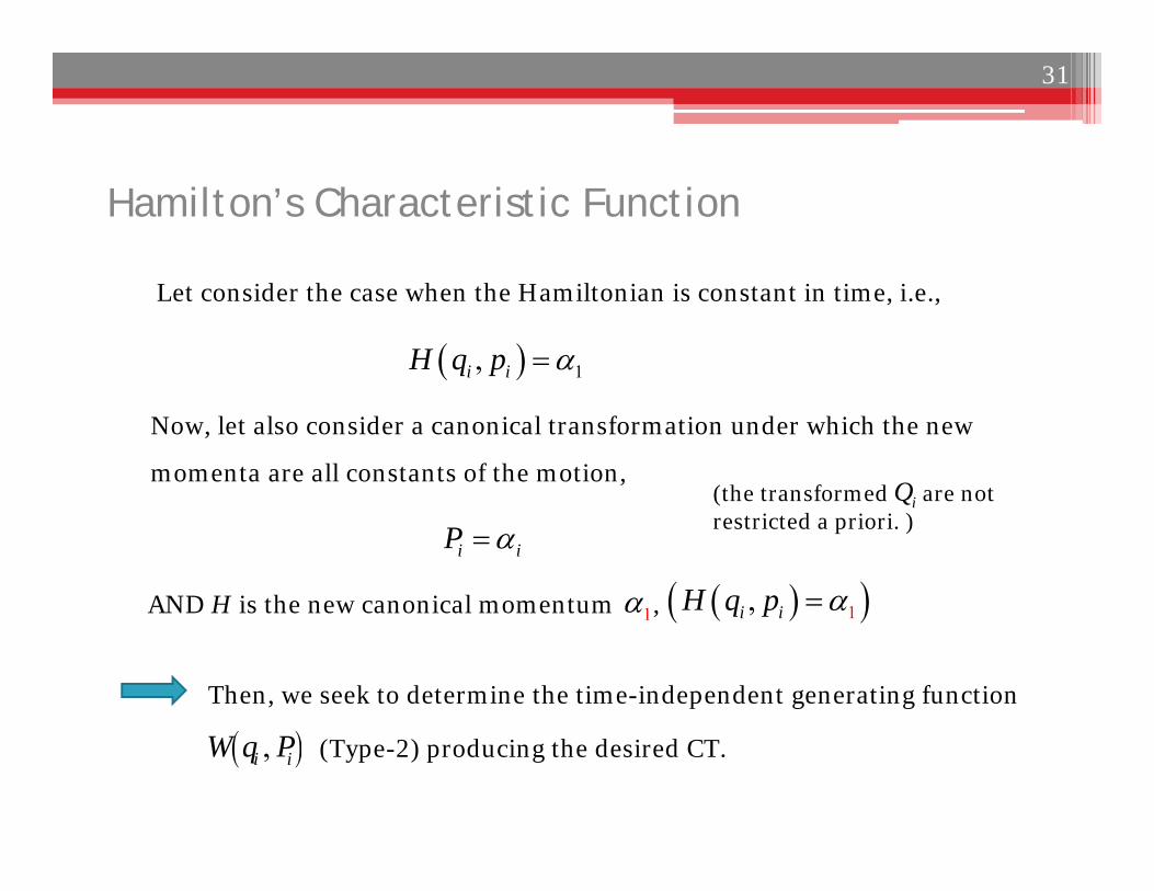
Hamilton’s Characteristic Function
Let consider the case when the Hamiltonian is constant in time, i.e.,
Now, let also consider a canonical transformation under which the new
momenta are all constants of the motion,
1,i iH q p
AND H is the new canonical momentum ,
31
i iP
1,i iH q p 1
Then, we seek to determine the time-independent generating function
(Type-2) producing the desired CT. ,i iW q P
(the transformed are not restricted a priori. )
iQ
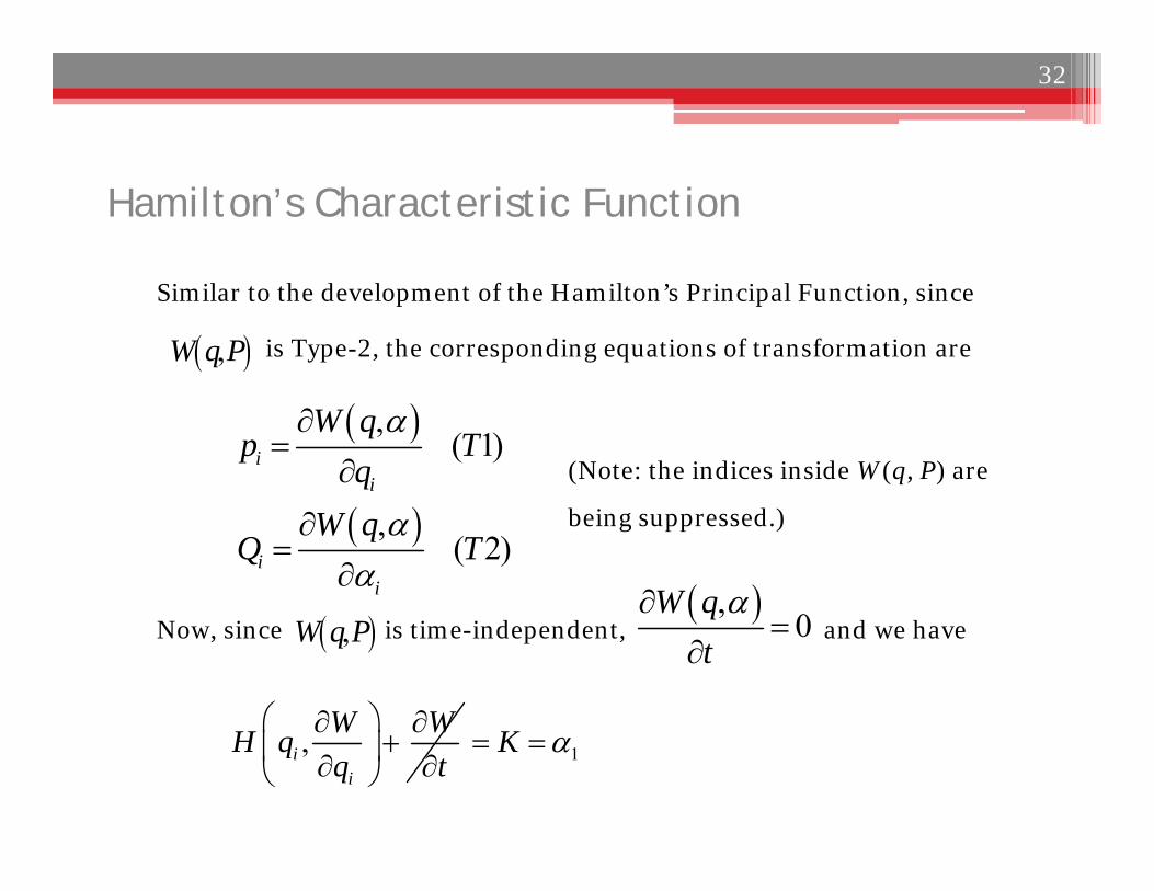
Hamilton’s Characteristic Function
Similar to the development of the Hamilton’s Principal Function, since
Now, since is time-independent, and we have
32
(Note: the indices inside W(q, P) are
being suppressed.)
,W q P
is Type-2, the corresponding equations of transformation are
,( 1)i
i
W qp T
q
,( 2)i
i
W qQ T
,
0W q
t
,ii
W WH qq t
1K
,W q P
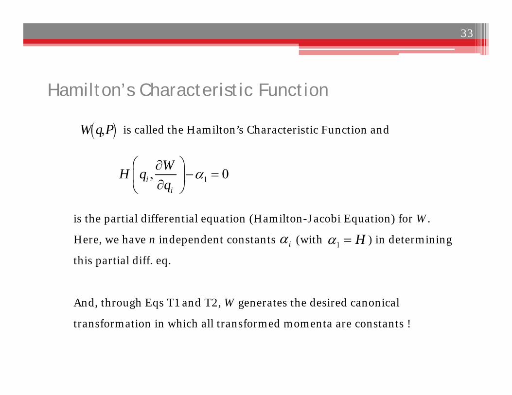
Hamilton’s Characteristic Function
is called the Hamilton’s Characteristic Function and
is the partial differential equation (Hamilton-Jacobi Equation) for W.
Here, we have n independent constants (with ) in determining
this partial diff. eq.
33
,W q P
1, 0ii
WH qq
And, through Eqs T1 and T2, W generates the desired canonical
transformation in which all transformed momenta are constants !
1 H i
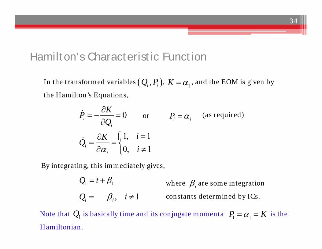
Hamilton’s Characteristic Function
In the transformed variables , , and the EOM is given by
the Hamilton’s Equations,
(as required)
34
0ii
KPQ
where are some integration
constants determined by ICs.
,i iQ P 1K
i iP or
1, 10, 1i
i
iKQi
1 1Q t
, 1i iQ i i
By integrating, this immediately gives,
Note that is basically time and its conjugate momenta is the
Hamiltonian.1Q 1 1P K
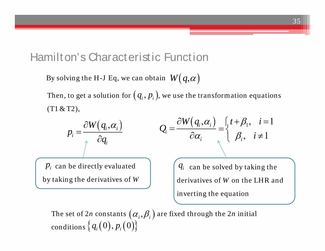
Hamilton’s Characteristic Function
Then, to get a solution for , we use the transformation equations
(T1 & T2),
35
can be directly evaluated
by taking the derivatives of W
,i iq p
By solving the H-J Eq, we can obtain
,i ii
i
W qp
q
,i ii
i
W qQ
,W q
ip
1, 1, 1i
t ii
can be solved by taking the
derivatives of W on the LHR and
inverting the equation
iq
The set of 2n constants are fixed through the 2n initial
conditions 0 , 0i iq p ,i i
Hamilton’s Characteristic Function
36
When the Hamiltonian does not dependent on time explicitly, one can use
either
- The Hamilton Principal Function or
- The Hamilton Characteristic Function ,W q P , ,S q P t
to solve a particular mechanics problem using the H-J equation and they
are related by:
1, , ,S q P t W q P t
Action-Angle Variables in 1dof
37
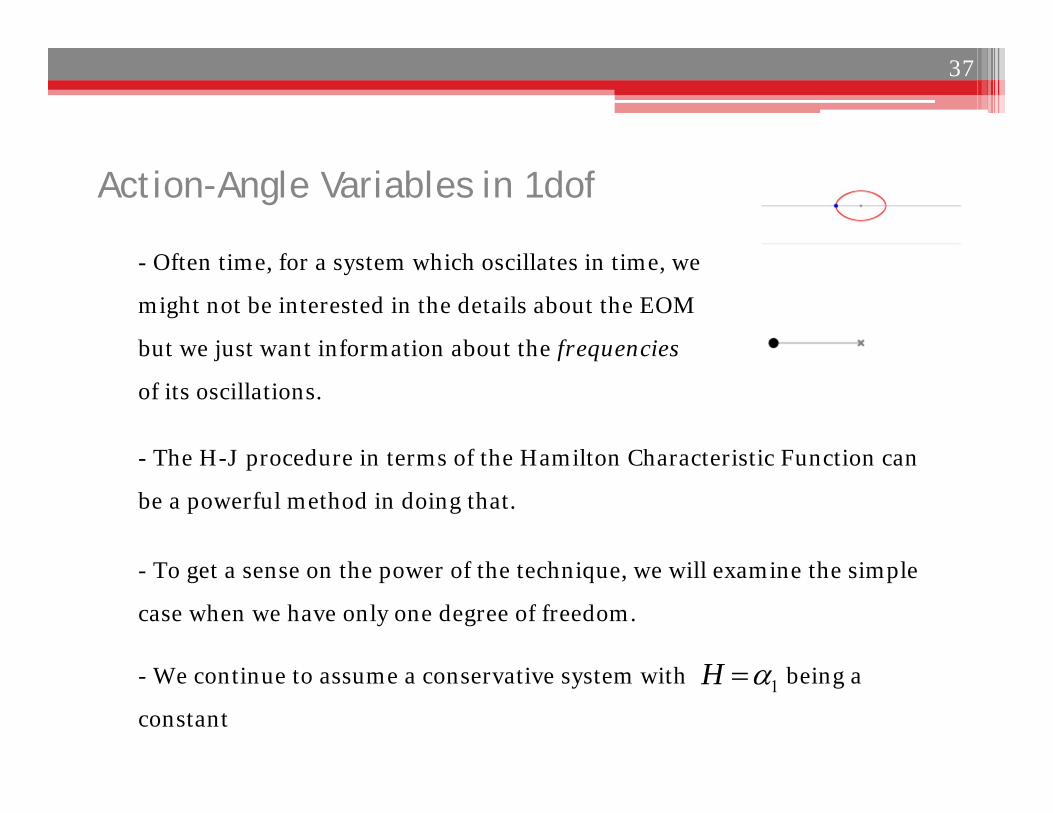
- Often time, for a system which oscillates in time, we
might not be interested in the details about the EOM
but we just want information about the frequencies
of its oscillations.
- The H-J procedure in terms of the Hamilton Characteristic Function can
be a powerful method in doing that.
- To get a sense on the power of the technique, we will examine the simple
case when we have only one degree of freedom.
- We continue to assume a conservative system with being a
constant1H
Action-Angle Variables in 1dof
38
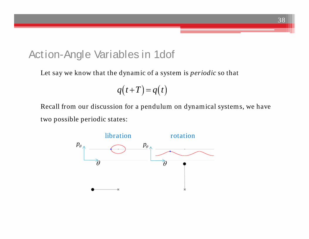
Let say we know that the dynamic of a system is periodic so that
Recall from our discussion for a pendulum on dynamical systems, we have
two possible periodic states:
q t T q t
libration rotation
p
p
Action-Angle Variables in 1dof
39
- Now, we introduce a new variable
called the Action Variable, where the path integral is taken over one full
cycle of the periodic motion.
J p dq
- Now, since the Hamiltonian is a constant, we have
1,H q p
- Then, by inverting the above equation to solve for p, we have
1,p p q
Action-Angle Variables in 1dof
40
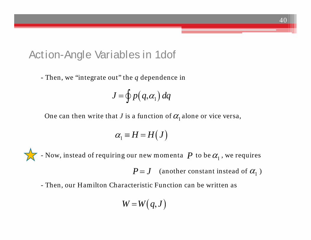
- Then, we “integrate out” the q dependence in
One can then write that J is a function of alone or vice versa,
1,J p q dq
- Now, instead of requiring our new momenta to be , we requires
1 H H J
- Then, our Hamilton Characteristic Function can be written as
,W W q J
1
1
P J (another constant instead of )1
P
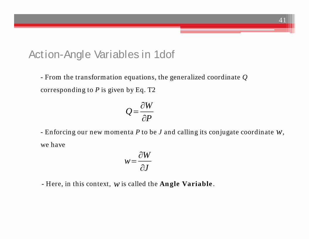
- Here, in this context, is called the Angle Variable.
Action-Angle Variables in 1dof
41
- From the transformation equations, the generalized coordinate Q
corresponding to P is given by Eq. T2
- Enforcing our new momenta P to be J and calling its conjugate coordinate ,
we have
WQP
w
WwJ
w
Action-Angle Variables in 1dof
42
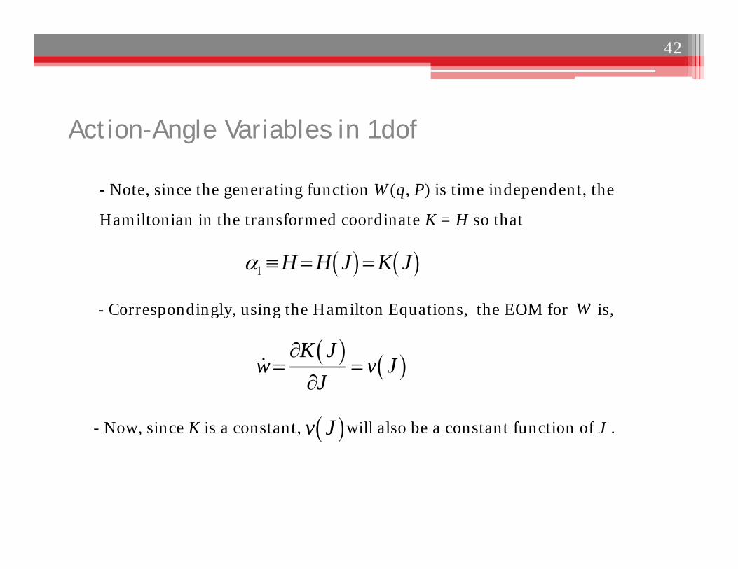
- Correspondingly, using the Hamilton Equations, the EOM for is,
- Note, since the generating function W(q, P) is time independent, the
Hamiltonian in the transformed coordinate K = H so that
K Jw v J
J
1 H H J K J
w
- Now, since K is a constant, will also be a constant function of J . v J
Action-Angle Variables in 1dof
43
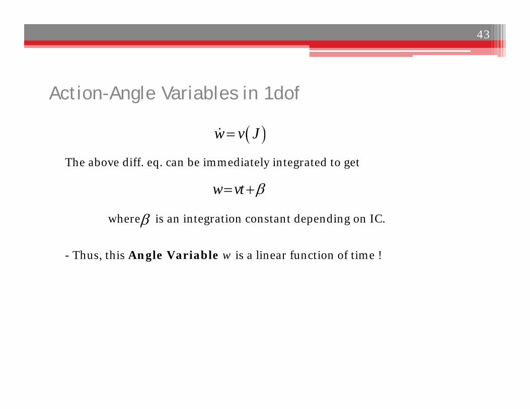
where is an integration constant depending on IC.
The above diff. eq. can be immediately integrated to get
w v J
w vt
- Thus, this Angle Variable w is a linear function of time !
Action-Angle Variables in 1dof
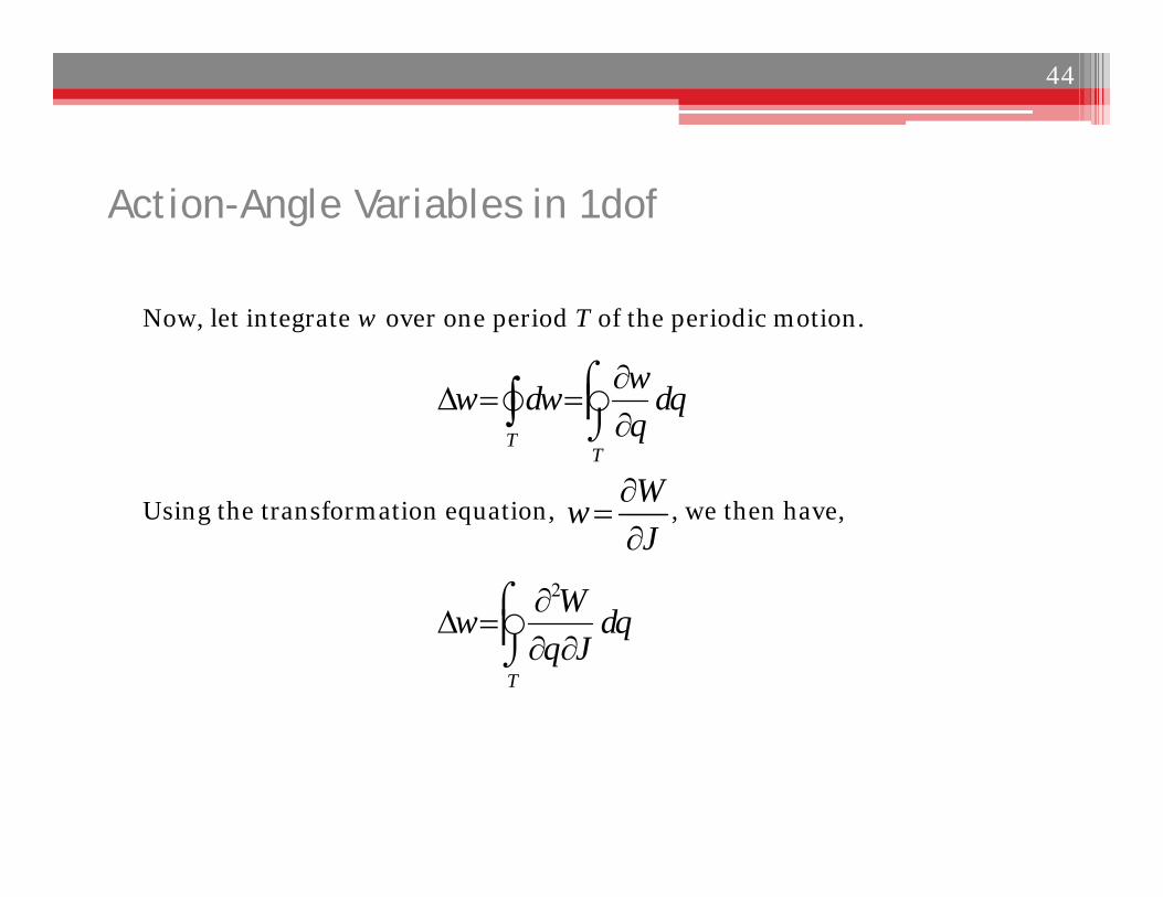
44
Using the transformation equation, , we then have,
Now, let integrate w over one period T of the periodic motion.
TT
ww dw dqq
WwJ
2
T
Ww dqq J
Action-Angle Variables in 1dof
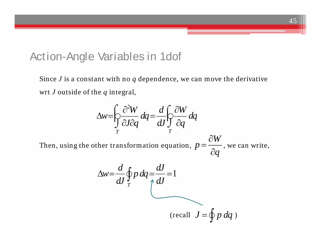
45
Then, using the other transformation equation, , we can write,
Since J is a constant with no q dependence, we can move the derivative
wrt J outside of the q integral,
2
TT
W d Ww dq dqJ q dJ q
Wpq
1T
d dJw p dqdJ dJ
(recall )J p dq
Action-Angle Variables in 1dof
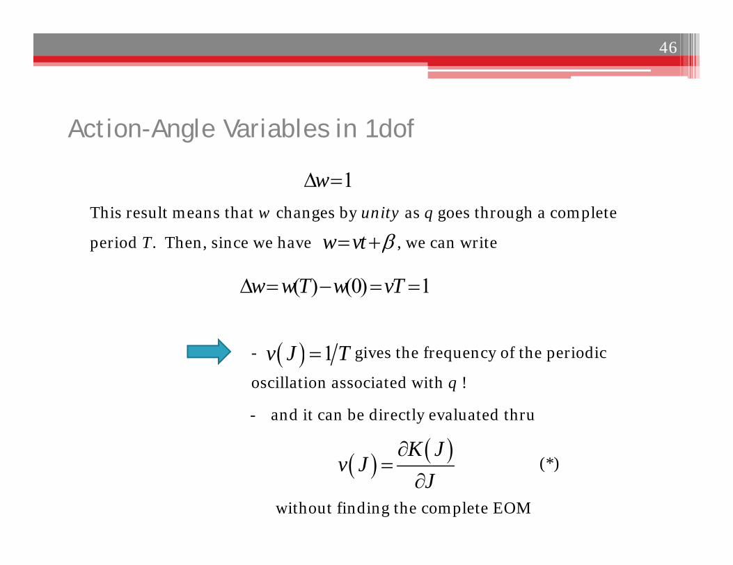
46
This result means that w changes by unity as q goes through a complete
period T. Then, since we have , we can write
1w
- gives the frequency of the periodic
oscillation associated with q !
w vt
( ) (0) 1w w T w vT
K Jv J
J
- and it can be directly evaluated thru
(*)
1v J T
without finding the complete EOM
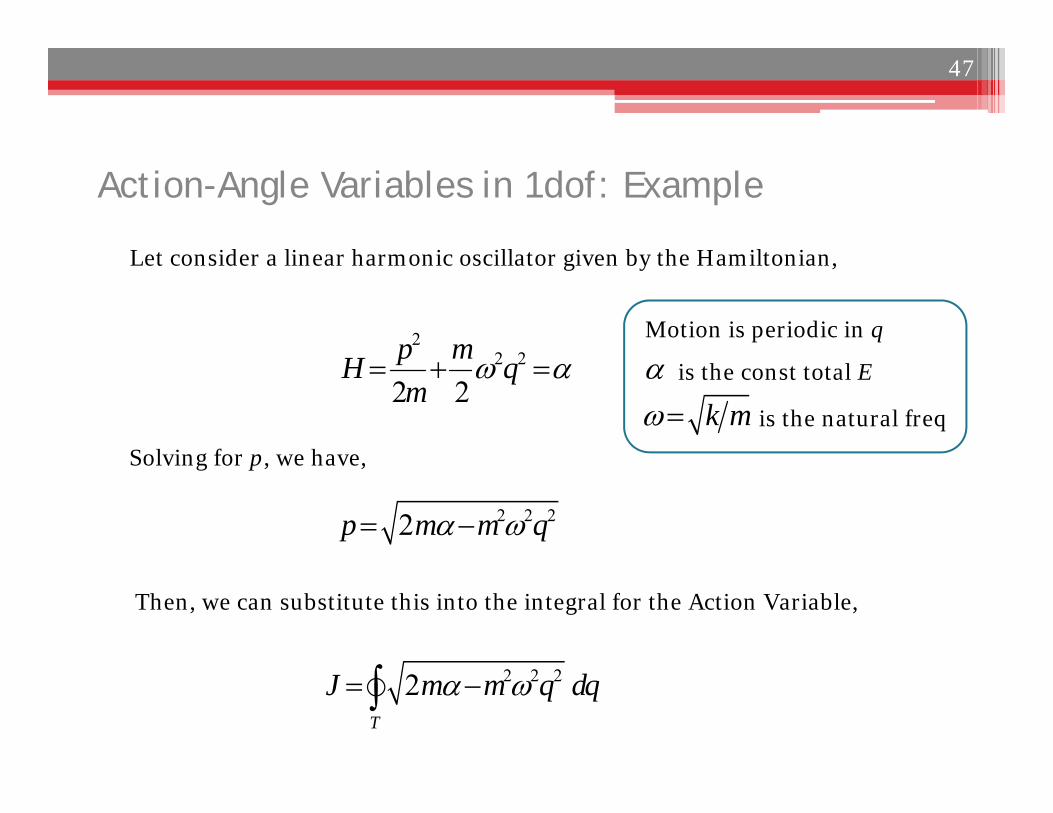
Action-Angle Variables in 1dof: Example
47
Let consider a linear harmonic oscillator given by the Hamiltonian,
22 2
2 2p mH qm
Solving for p, we have,
2 2 22p m m q
Then, we can substitute this into the integral for the Action Variable,
2 2 22T
J m m q dq
is the const total E
is the natural freq
k m
Motion is periodic in q
Action-Angle Variables in 1dof: Example
48
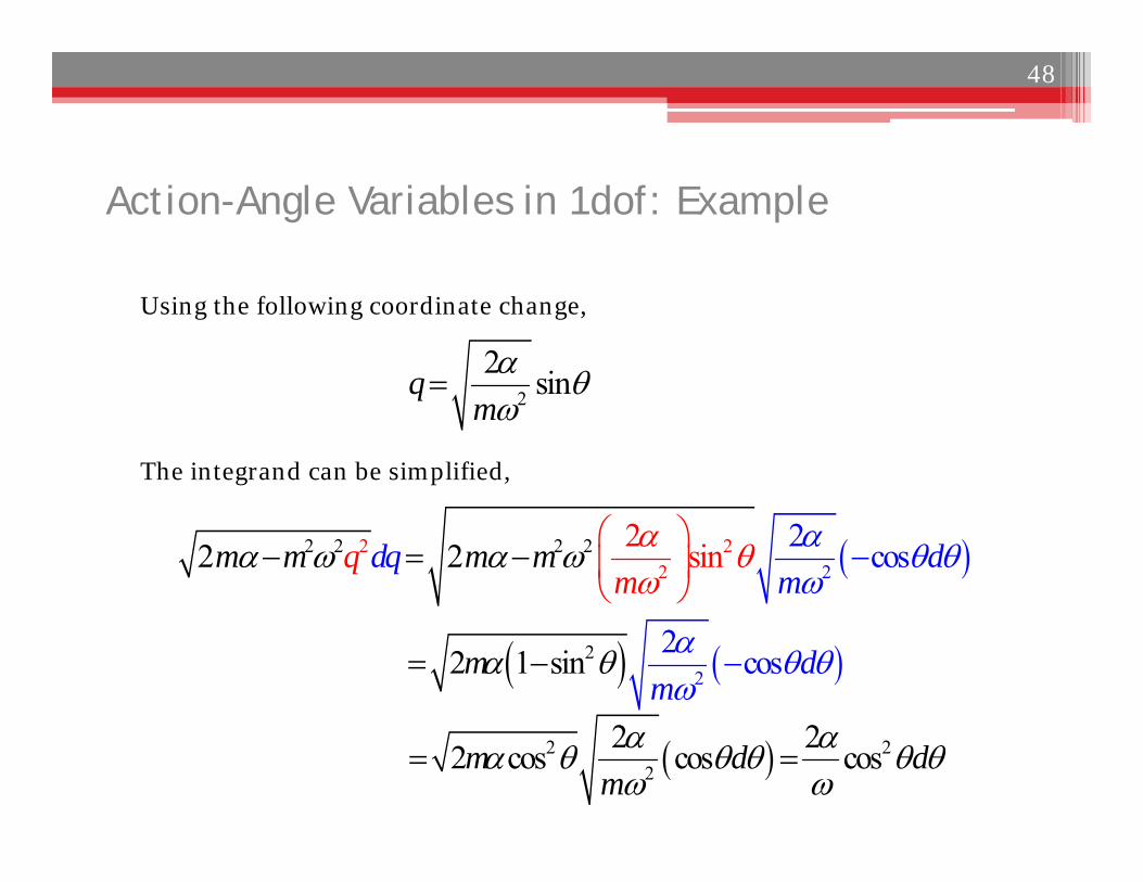
Using the following coordinate change,
2
2 sinqm
The integrand can be simplified,
22 2
22 2 2 2 2 s 2 co2 i2 n sm m m m
mq
mdq d
22
22 1 si cn os dm
m
2 22
2 22 cos cos cosm d dm
Action-Angle Variables in 1dof: Example
49
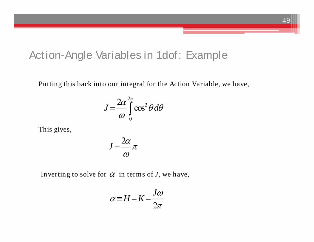
Putting this back into our integral for the Action Variable, we have,
This gives,
22
0
2 cosJ d
2J
Inverting to solve for in terms of J, we have,
2JH K
Action-Angle Variables in 1dof: Example
50
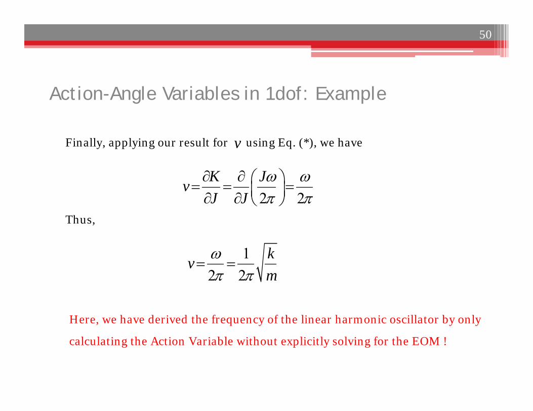
Finally, applying our result for using Eq. (*), we have
Thus,
2 2K JvJ J
12 2
kvm
v
Here, we have derived the frequency of the linear harmonic oscillator by only
calculating the Action Variable without explicitly solving for the EOM !