Embed Size (px)
Citation preview

For Peer R
eview
!"#$%&'&(&)"&'*'+'*%(,#$,-$#*'."(/'*0'"(#"(1"&)23$)(4#$2#"(
5'$*)6! "#$%&'()! !"#$%&$'()*+"$,#')+-)%.&)/+(#')0&%&+$+'+123#')4+32&%(!
*'&$+,%-./!01)! 2"34534456789!
:-(;<!3!*'&$+,%-./!/<.;)! 8;+;'%,=!>%/-,(;!
1'/;!?$@A-//;B!@<!/=;!>$/=#%)!
C#A.(;/;!D-+/!#E!>$/=#%+)! D-$F!"$&G-;H!I&-J;%+-/<!#E!*'%<('&BF!>/A#+.=;%-,!'&B!K,;'&-,!
?,-;&,;!L'(&'<F!M$N;&-'H!I&-J;%+-/<!#E!*'%<('&BF!>/A#+.=;%-,!'&B!K,;'&-,!?,-;&,;!*-<#+=-F!O'P;A'+'H!I&-J;%+-/<!#E!*'%<('&BF!>/A#+.=;%-,!'&B!
K,;'&-,!?,-;&,;!C'%B-&'(-F!C'%('H!MC*:Q!
L;<R#%B+)! >&'(<+-+!+;&+-/-J-/<F!M&+;A@(;!L'(A'&!E-(/;%F!C%#++!S'(-B'/-#&!
Quarterly Journal of the Royal Meteorological Society

For Peer R
eview
1
Analysis sensitivity calculation in Ensemble Kalman Filter
Junjie Liu1, Eugenia Kalnay
2, Takemasa Miyoshi
2, and Carla Cardinali
3
1University of California, Berkeley, CA, USA
2University of Maryland, College Park, MD, USA
3ECMWF, Data Assimilation Section, Reading, UK
Page 2 of 30 Quarterly Journal of the Royal Meteorological Society
1
2
3
4
5
6
7
8
9
10
11
12
13
14
15
16
17
18
19
20
21
22
23
24
25
26
27
28
29
30
31
32
33
34
35
36
37
38
39
40
41
42
43
44
45
46
47
48
49
50
51
52
53
54
55
56
57
58
59
60

For Peer R
eview
2
Abstract
Analysis sensitivity indicates the sensitivity of analysis to observations, which is
complementary to the sensitivity of the analysis to background. Following Cardinali et al.
(2004), this paper discussed a method to calculate this quantity in Ensemble Kalman
Filter without approximations. The calculation procedure and the geometrical
interpretation showing that analysis sensitivity is proportional to analysis error and anti-
correlated with observation error are experimentally verified with the Lorenz-40 variable
model. Cross-validation in its original formulation (Wahba, 1990) is computationally
unfeasible even for a model with a moderate number of degrees of freedom, but is
computed efficiently using analysis sensitivity in an EnKF.
Idealized experiments based on a simplified-parameterization primitive equation
global model show that information content (trace of analysis sensitivity of any subset of
observations) agrees qualitatively with the actual observation impact calculated from
much more expensive data denial experiments, not only for the same type of dynamical
variable, but also for different types of dynamical variables.
Page 3 of 30Quarterly Journal of the Royal Meteorological Society
1
2
3
4
5
6
7
8
9
10
11
12
13
14
15
16
17
18
19
20
21
22
23
24
25
26
27
28
29
30
31
32
33
34
35
36
37
38
39
40
41
42
43
44
45
46
47
48
49
50
51
52
53
54
55
56
57
58
59
60

For Peer R
eview
3
1. Introduction
Observations are the central information introduced into numerical weather
prediction system through data assimilation; a process that combines observations with
background forecasts based on their error statistics. With the increase of observation
datasets assimilated in modern data assimilation systems, such as the assimilation of
Advanced InfraRed Satellite (AIRS) and the Infrared Atmospheric Sounding
Interferometer (IASI), it is important to examine questions such as how much
information content a new observation dataset has, what is the spatial distribution of the
impact of the new observations on the analysis, and what is the relative influence of
background forecasts and observations on the analyses.
The computation of analysis sensitivity (also called as self-sensitivity), a quantity
introduced by Cardinali et al. (2004) can address these questions. The larger the analysis
sensitivity is, the larger is the influence of observations, and the smaller the influence of
background forecasts. Since analysis sensitivity is a function of the analysis error
covariance that is not explicitly calculated in variational data assimilation schemes,
Cardinali et al. (2004) proposed an approximate method to calculate this quantity within a
4D-Var data assimilation framework. They showed that the trace of analysis sensitivity of
a particular observation data type represented the information content of that type of
observations, and the relative importance of different observation types determined by
information content was in good qualitative agreement with the observation impact from
other studies. In addition, information content has also been used in channel selection in
multi-thousand channel satellite instruments, such as in IASI (Rabier et al., 2002).
Page 4 of 30 Quarterly Journal of the Royal Meteorological Society
1
2
3
4
5
6
7
8
9
10
11
12
13
14
15
16
17
18
19
20
21
22
23
24
25
26
27
28
29
30
31
32
33
34
35
36
37
38
39
40
41
42
43
44
45
46
47
48
49
50
51
52
53
54
55
56
57
58
59
60

For Peer R
eview
4
Though the approximate method to calculate analysis sensitivity within 4D-Var is
computationally possible, it introduces spurious values that are not within the theoretical
value range (between 0 and 1). In contrast with variational data assimilation schemes,
Ensemble Kalman filters (EnKF) (Evensen, 1994; Anderson, 2001; Bishop et al., 2001;
Houtekamer and Mitchell, 2001; Whitaker and Hamill, 2002; Ott et al., 2004; Hunt et al.,
2007) generate ensemble analyses that can be used to calculate the analysis error
covariance. Because of this characteristic, it would be more straightforward to calculate
analysis sensitivity in EnKF than in variational data assimilation. In addition, the Cross
Validation (CV) (Wahba, 1990) score can be exactly calculated in EnKF based on the
analysis sensitivity, observation and analysis values without carrying out data denial
experiments (section 4). In the variational formulation, because of the approximations
made in calculating analysis sensitivities, cross-validation cannot be exactly computed. In
this paper, we follow Cardinali et al. (2004), show how to calculate analysis sensitivity
and the related diagnostics in EnKF, and further study the properties and possible
applications of these diagnostics. This paper is organized as follows: section 2 describes
how to calculate analysis sensitivity in EnKF. In section 3, with a geometrical
interpretation method adapted from Desroziers et al. (2005), we show that analysis
sensitivity is proportional to the analysis errors and anti-correlated with the observation
errors. With the Lorenz-40 variable model (Lorenz and Emanuel, 1998), section 4
verifies the self-sensitivity calculation procedure, and shows the squared analysis value
change based on analysis sensitivity can differentiate abnormal observations from normal
ones. In addition, the geometrical interpretation is experimentally tested in this section. In
section 5, with a primitive equation model and a perfect model experimental setup (no
Page 5 of 30Quarterly Journal of the Royal Meteorological Society
1
2
3
4
5
6
7
8
9
10
11
12
13
14
15
16
17
18
19
20
21
22
23
24
25
26
27
28
29
30
31
32
33
34
35
36
37
38
39
40
41
42
43
44
45
46
47
48
49
50
51
52
53
54
55
56
57
58
59
60

For Peer R
eview
5
model error), we examine the effectiveness of the trace of self-sensitivity in assessing the
observation impact obtained from data denial experiments. Section 6 contains a summary
and conclusions.
2. Calculation of analysis sensitivity in EnKF
In this section, we first briefly derive the analysis sensitivity valid for all data
assimilation schemes (equations (1), (2), (3), equivalent to equations (3.1), (3.4), and
(3.5) in Cardinali et al., 2004) and then focus on how to calculate this quantity in EnKF.
In data assimilation, the analysis state ax combines the background (an n-
dimensional vector bx ) and the observations (a p-dimensional vector o
y ) based on a
weighting matrix K , which can be expressed as:
b
n
oaxKHIKyx )( !+= (1)
The (n ! p) gain matrix K = PbH
T(HP
bH
T+ R)
!1 weighs the error covariance of the
background Pb
and of the observations R , and H(•) is the linearized observation
operator that transforms a perturbation from model space to observation space. From
Equation (1), the analysis sensitivity with respect to observations is:
TaTT
o
a
oHHPRHK
y
yS
1ˆ
!==
"
"= , (2)
and the sensitivity with respect to background is given by
o
p
TT
pb
ab
SIHKIy
yS !=!=
"
"=ˆ
(3)
where ya = Hxa = HKyo + (I p !HK)yb is the projection of analysis (equation (1)) on
observation space, and bbHxy = is the projection of background on observation space.
Page 6 of 30 Quarterly Journal of the Royal Meteorological Society
1
2
3
4
5
6
7
8
9
10
11
12
13
14
15
16
17
18
19
20
21
22
23
24
25
26
27
28
29
30
31
32
33
34
35
36
37
38
39
40
41
42
43
44
45
46
47
48
49
50
51
52
53
54
55
56
57
58
59
60

For Peer R
eview
6
Pa= P
bH
T(HP
bH
T+ R)
!1 is the analysis error covariance. The matrix oS is called
influence matrix, because the elements of this matrix reflect how much influence the
observations have on the analysis state. The diagonal elements of the matrix oS are
analysis self-sensitivities, and the off-diagonal elements are cross sensitivities. Similarly
b
a
y
y
!
!ˆ reflects how much influence the background has on the analysis. As shown in
Cardinali et al. (2004), the self-sensitivity of the analysis with respect to observation and
the corresponding background at that observation location are complementary (i.e., they
add up to one), and self-sensitivity has no unit and its theoretical value is between 0 and 1
when the observation errors are not correlated (R is diagonal).
EnKF generates ensemble analyses in every analysis cycle, and the analysis error
covariance can be written as products of ensemble analysis perturbations, so in EnKF
equation (2) can be written as:
So= R
!1HP
aH
T=
1
n !1R
!1(HX
a)(HX
a)T (4)
where HXais the analysis ensemble perturbation matrix in the observation space whose
thi column is
HX
ai! h(x
ai) "1
nh(x
ai)
i=1
n
# (5)
xai
is the thi analysis ensemble member, n is the total number of ensemble analyses, and
h(•) is the observation operator, which can be linear or nonlinear. When the observation
operator is linear, the right hand side and the left hand side of Equation (5) are exactly
equal. Otherwise, the left hand side is a linear approximation of the right hand side. When
the observation errors are not correlated, the self-sensitivity can be written as:
Page 7 of 30Quarterly Journal of the Royal Meteorological Society
1
2
3
4
5
6
7
8
9
10
11
12
13
14
15
16
17
18
19
20
21
22
23
24
25
26
27
28
29
30
31
32
33
34
35
36
37
38
39
40
41
42
43
44
45
46
47
48
49
50
51
52
53
54
55
56
57
58
59
60

For Peer R
eview
7
Sjjo=!y j
a
!y jo=
1
n "1#$%
&'(1
) j
2(HX
ai) jT(HX
ai) j
i=1
n
* (6)
and the cross sensitivity, which represents the change of yj
a with respect to the variation
of observation ylo , can be written as:
Sjlo=!y j
a
!ylo=
1
n "1#$%
&'(1
) j
2[(HX
ai) jT(HX
ai)l ]
i=1
n
* (7)
where !j
2 is the j th observation error variance. Equation (5) indicates that the calculation
of the self-sensitivity and cross sensitivity in EnKF only requires applying the
observation operator on each analysis ensemble member, and then doing scalar
calculation based on equations (6) and (7). In section 4, this calculation procedure will be
verified with the Lorenz-40 variable model. The calculation of the self-sensitivity based
on equation (6) requires no approximations when the observation errors are not
correlated, so thatSjjo satisfies the theoretical value limits (between 0 and 1). In 4D-Var,
by contrast, the calculation of analysis error covariance is based on a truncated
eigenvector expansion with vectors obtained through the Lanczos algorithm, which can
introduce spurious values larger than one (Cardinali et al., 2004).
3. Geometric interpretation of self-sensitivity
Equations (6) shows that the analysis sensitivity is proportional to the analysis
error variance and inversely proportional to the observation error variance. Since in most
cases, the analysis and observation error statistics used in data assimilation do represent
the accuracy of analyses and observations respectively, equation (6) implicitly indicates
that analysis sensitivity increases with the analysis errors and decreases with the
Page 8 of 30 Quarterly Journal of the Royal Meteorological Society
1
2
3
4
5
6
7
8
9
10
11
12
13
14
15
16
17
18
19
20
21
22
23
24
25
26
27
28
29
30
31
32
33
34
35
36
37
38
39
40
41
42
43
44
45
46
47
48
49
50
51
52
53
54
55
56
57
58
59
60

For Peer R
eview
8
observation errors. In this section, we adapt the geometrical interpretation that Desroziers
et al. (2005) used to explain the relationship among background error, observation error
and analysis error to further show this relationship in the space of eigenvectors V of the
matrix HK .
Following the same notation as Desroziers et al. (2005), we rewrite equation
ya = HKyo + (I p !HK)yb by subtracting h(xt ) , the true state in observation space, from
both sides and obtain
ya ! h(xt ) = HK(yo ! h(xt )) + (I p !HK)(yb! h(xt )) (8)
In equation (8), ! ya = ya " h(xt ) , !yb = yb " h(xt ) and !yo = yo " h(xt )are analysis and
background errors in observation space, and observation errors respectively. Then
equation (8) can be written as,
b
p
oayHK(IyHKy !!! )ˆ "+= (9)
Following Desroziers et al. (2005), we give a geometrical interpretation in the space of
eigenvectors V of the matrix HK , so that HK = V!VT
where ! is a diagonal matrix
composed of the eigenvalues of HK . The projections of ay! onto the eigenvector V is
given by VT! ya = VTV"VT
!yo + VTV(I p # ")VT!yb , which can be further written as
! ˆ!
ya = "!!yo + (I p # ")!
!yb (10)
! ˆ!
ya ,
!!yo and
!!yb are analysis, observation, and background error in the eigenvector
space V respectively, and are the projections of ! ya , !yo and !yb on the eigenvector V
space. When these vectors are projected on a particular eigenvector Vi
with
corresponding eigenvalue equal to !i, the above equation can be written as,
Page 9 of 30Quarterly Journal of the Royal Meteorological Society
1
2
3
4
5
6
7
8
9
10
11
12
13
14
15
16
17
18
19
20
21
22
23
24
25
26
27
28
29
30
31
32
33
34
35
36
37
38
39
40
41
42
43
44
45
46
47
48
49
50
51
52
53
54
55
56
57
58
59
60
For Peer R
eview
9
! ˆ!
yi
a= "
i!!yi
o+ (1# "
i)!!yi
b (11)
Therefore, in the eigenvector iV space, the analysis sensitivity with respect to the
observation is !i, and with respect to the background is (1-!
i). As shown in Cardinali et
al. (2004), they are complementary with diagonal observation error covariance.
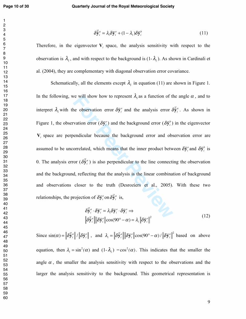
Schematically, all the elements except !i in equation (11) are shown in Figure 1.
In the following, we will show how to represent !ias a function of the angle ! , and to
interpret !iwith the observation error
!!yo
i and the analysis error
! ˆ!
yi
a . As shown in
Figure 1, the observation error ( !!yo
i) and the background error (
!!yb
i) in the eigenvector
iV space are perpendicular because the background error and observation error are
assumed to be uncorrelated, which means that the inner product between !!yo
iand
!!yb
i is
0. The analysis error ( ! ˆ!
yi
a ) is also perpendicular to the line connecting the observation
and the background, reflecting that the analysis is the linear combination of background
and observations closer to the truth (Desroziers et al., 2005). With these two
relationships, the projection of !!yo
ion
! ˆ!
ya
i is,
! ˆ!
yi
a"!!yi
o= #
i!!yi
o"!!yi
o$
! ˆ!
yi
a!!yi
ocos(90° %& ) = #
i!!yi
o2 (12)
Since sin(! ) = " ˆ
!
yi
a/ "!yi
o , and !i= " ˆ!
yi
a"!yi
ocos(90° #$ ) / "
!yi
o2
based on above
equation, then !i= sin
2(" ) and (1-!
i) = cos2 (! ) . This indicates that the smaller the
angle ! , the smaller the analysis sensitivity with respect to the observations and the
larger the analysis sensitivity to the background. This geometrical representation is
Page 10 of 30 Quarterly Journal of the Royal Meteorological Society
1
2
3
4
5
6
7
8
9
10
11
12
13
14
15
16
17
18
19
20
21
22
23
24
25
26
27
28
29
30
31
32
33
34
35
36
37
38
39
40
41
42
43
44
45
46
47
48
49
50
51
52
53
54
55
56
57
58
59
60

For Peer R
eview
10
consistent with equation (6) showing that analysis sensitivity per observation increases
with the analysis error and decreases with the observation error.
Figure 1 Geometrical representation of the vector elements in equation (11) (see text). The
analysis sensitivity with respect to the observations is sin2! (adapted from Desroziers et al.,
2005).
4. Validation of the self-sensitivity calculation method in EnKF and cross validation
experiments with the Lorenz 40-variable model
Cardinali et al. (2004) showed that the change in the analysis yi
a obtained by
leaving out the ith
observation could be calculated from the self-sensitivity Sii
o , yi
o and
yi
a without calculating yi
a(! i ) (the estimate of yi
a obtained by leaving out the
ith
observation), and that the same was true for the calculation of Cross Validation (CV)
score (Wahba, 1990, theorem 4.2.1), which is traditionally obtained from leaving out
each observation in turn and is defined as (yi
o! y
i
a(! i ))2
i=1
m
" , m is the total observations.
Page 11 of 30Quarterly Journal of the Royal Meteorological Society
1
2
3
4
5
6
7
8
9
10
11
12
13
14
15
16
17
18
19
20
21
22
23
24
25
26
27
28
29
30
31
32
33
34
35
36
37
38
39
40
41
42
43
44
45
46
47
48
49
50
51
52
53
54
55
56
57
58
59
60

For Peer R
eview
11
Therefore, to verify the self-sensitivity calculation method in EnKF (Equation (5)), we
will compare yi
o! y
i
a(! i ) and CV score based on the actual computation of yi
a(! i ) to those
from self-sensitivity following equations (2.9) and (2.10) in Cardinali et al. (2004):
yia! yi
a(! i )=
Siio
(1! Siio)(yi
o! yi
a) (13)
(yi
o! yi
a(! i ))2
i=1
m
" =(yi
o! yi
a)2
(1! Siio)2
i=1
m
" (14)
With a correct estimation of the self-sensitivity, the left and the right hand sides of
equations (13) and (14) should be equal. Deleting each observation in turn is
computationally formidable in a realistic NWP data assimilation system, so we use the
Lorenz-40 variable for this purpose. It is important to note that the left hand side of
Equation (13) estimates the changes that each observation introduces on the analysis. We
expect that the analysis change yi
a! y
i
a(! i ) with and without the ith
observation will be
abnormally large in data sparse regions, or when the atmosphere is unusually sensitive to
small perturbations (in the presence of a bifurcation), or when the observation errors are
very large. By contrast, we expect the analysis changes to be small in data rich regions. In
this section, we will use this characteristic to detect an observation that changes
substantially the analysis in a uniform observation coverage scenario without carrying out
the denial experiment.
4.1 Lorenz-40 variable model and experimental setup
The Lorenz 40-variable model is governed by the following equation:
Page 12 of 30 Quarterly Journal of the Royal Meteorological Society
1
2
3
4
5
6
7
8
9
10
11
12
13
14
15
16
17
18
19
20
21
22
23
24
25
26
27
28
29
30
31
32
33
34
35
36
37
38
39
40
41
42
43
44
45
46
47
48
49
50
51
52
53
54
55
56
57
58
59
60

For Peer R
eview
12
Fxxxxx
dt
djjjjj +!!=
!!+ 121 )( (15)
The variables ( jx , j=1…J) represent a “meteorological” variable on a “latitude circle”
with periodic boundary conditions. As in Lorenz and Emanuel (1998), J is chosen to be
40. The time step is 0.05, which corresponds to a 6-hour integration interval. F is the
external forcing, which is 8 for the nature run, and 7.6 for the forecast, allowing for some
model error in the system. Observations are simulated by adding to the nature run
Gaussian random perturbations with standard deviation equal to 0.2.
The data assimilation scheme we use is the Local Ensemble Transform Kalman
Filter (LETKF), which is one type of EnKF specifically efficient for parallel computing
(see Hunt et al. (2007) for a detailed description of this method). Since F has different
values in the nature run and forecast, multiplicative covariance inflation (Anderson and
Anderson, 1999) has been applied to account for the model error in addition to the
sampling errors. The covariance inflation factor is fixed to be 1.3 in this study, which
means that background error covariance Pb is multiplied by 1.3 during data assimilation.
In verifying self-sensitivity calculation method, we use 40 ensemble members, and
assume full observation coverage. The analysis sensitivity Sii
o is calculated after each
analysis cycle based on equation (6). After full observation data assimilation, each
observation is left out in turn to get yi
a(! i ) using the same background forecasts. To
experimentally examine the relationship among analysis sensitivity per observation,
observation coverage, and analysis accuracy, we carry out several uniform observation
coverage scenarios, namely, 20, 25, 30, 35 and 40 observations. Analysis accuracy is
measured by Root Mean Square (RMS) error, which is defined as the RMS difference
Page 13 of 30Quarterly Journal of the Royal Meteorological Society
1
2
3
4
5
6
7
8
9
10
11
12
13
14
15
16
17
18
19
20
21
22
23
24
25
26
27
28
29
30
31
32
33
34
35
36
37
38
39
40
41
42
43
44
45
46
47
48
49
50
51
52
53
54
55
56
57
58
59
60

For Peer R
eview
13
between analysis mean value and the nature run. In order to show that the square of the
analysis value change based on the right hand of equation (13) could detect unusual
observations, we assign to the observation at the 11th
point random errors 4 times larger
than to the other observations as in Liu and Kalnay (2008). Since the observation error at
the 11th point is much larger than the other points, the square of the analysis value change
would be larger than at the other points. For statistic significance of the results, we run
each experiment for 1000 analysis cycles, and calculate a time average over the last 500
analysis cycles.
4.2 Results
Comparison between yi
a! y
i
a(! i ) and
Siio
(1! Siio)(yi
o! yi
a) at a single analysis time
(top panel in Figure 2) shows that they have the same value at every grid point,
confirming the validity of equation (13). This is also true for the comparison between the
cross validation score based on deleting each observation in turn (plus signs in the bottom
panel of Figure 2) and that from the self-sensitivity (open circles in the bottom panel of
Figure 2). These comparisons prove that the calculation of the self-sensitivity based on
equation (6) in EnKF is valid, and that a complete cross-validation that would be
unfeasible with the standard approach, can be computed within the ensemble data
assimilation cycle based on self-sensitivity. Further experiments with different
observation coverage support this conclusion.
Figure 3 shows that self-sensitivity increases with the analysis RMS error, which
is consistent with the geometrical interpretation in section 3. Since analysis error is anti-
correlated with observation coverage, so is self-sensitivity (Figure 3). The analysis
Page 14 of 30 Quarterly Journal of the Royal Meteorological Society
1
2
3
4
5
6
7
8
9
10
11
12
13
14
15
16
17
18
19
20
21
22
23
24
25
26
27
28
29
30
31
32
33
34
35
36
37
38
39
40
41
42
43
44
45
46
47
48
49
50
51
52
53
54
55
56
57
58
59
60

For Peer R
eview
14
sensitivity per observation becomes larger when the observation coverage becomes
sparser. The analysis sensitivity per observation is about 0.16 when all the grid points are
observed, which indicates that 16% of the information in the analysis comes from the
observation at each location. Since the analysis sensitivity with respect to the background
is complementary to the analysis sensitivity with respect to the observation (section 3),
84% information of the analysis comes from the background forecast. When only half
grid points have observations, the analysis self-sensitivity is about 0.32, which indicates
that deletion of one observation in dense observation coverage will do less harm to the
analysis system than deletion of one observation in a sparse case. This is consistent with
field experiments (e.g., Kelly et al., 2007).
The time-average of the squared analysis value change ( (yi
a! y
i
a(! i ))2 ) based on
the right hand side of equation (13) shows the mean squared change at the 11th point,
which has 4 times larger random error than the other points, is abnormally large. This
confirms that the squared analysis value change based on analysis sensitivity can be used
to detect abnormal observations very efficiently at the analysis time, without performing
data denial experiments. In a real NWP scenario, in which the observation coverage is not
uniform, an abnormal behavior of the observations based on the change of the analysis
value may come from the non-uniform observation coverage: the value should be larger
in data sparse areas. However, since the calculation of the absolute analysis value change
based on equation (13) is very simple and requires little computational time, it could be
used as a sophisticated observation quality check.
Page 15 of 30Quarterly Journal of the Royal Meteorological Society
1
2
3
4
5
6
7
8
9
10
11
12
13
14
15
16
17
18
19
20
21
22
23
24
25
26
27
28
29
30
31
32
33
34
35
36
37
38
39
40
41
42
43
44
45
46
47
48
49
50
51
52
53
54
55
56
57
58
59
60

For Peer R
eview
15
Figure 2 Top panel: yi
a! y
i
a(! i )(plus sign) and
Sii
o
(1! Sii
o)ri(open circles) comparison at one
analysis time as function of grid point. Bottom panel: comparison of CV score calculated
from (yi
o! y
i
a(! i ))2
i=1
m
" (plus sign) and that from (yi
o! yi
a)2
(1! Siio)2
i=1
m
" (open circles) in the first 60
analysis cycles.
Page 16 of 30 Quarterly Journal of the Royal Meteorological Society
1
2
3
4
5
6
7
8
9
10
11
12
13
14
15
16
17
18
19
20
21
22
23
24
25
26
27
28
29
30
31
32
33
34
35
36
37
38
39
40
41
42
43
44
45
46
47
48
49
50
51
52
53
54
55
56
57
58
59
60

For Peer R
eview
16
Figure 3 Scatter plot of the time averaged analysis sensitivity per observation (y-axis) and
the analysis RMS error (x-axis) (from bottom to top, the points correspond to 40
observations, 35 observations, 30 observation, 25 observation and 20 observations).
Figure 4 Time average of the squared analysis value change (equation (13)) by leaving out
each observation in turn. The observation error at the 11th
point is four times larger than
the errors of the other observations.
5. Consistency between information content and the observation impact obtained
from data denial experiments
Equation (13) indicates that the deletion of an observation with larger self-
sensitivity will result in larger change in the analysis value compared to the deletion of
Page 17 of 30Quarterly Journal of the Royal Meteorological Society
1
2
3
4
5
6
7
8
9
10
11
12
13
14
15
16
17
18
19
20
21
22
23
24
25
26
27
28
29
30
31
32
33
34
35
36
37
38
39
40
41
42
43
44
45
46
47
48
49
50
51
52
53
54
55
56
57
58
59
60

For Peer R
eview
17
other observations. Assuming that the correction to the analysis by that observation is to
make analysis better, which is true statistically when error statistics used in data
assimilation are correct, the deletion of that observation will result in a worse analysis
than the deletion of other observations. Equation (13) is only valid when one observation
is left out. However, in most NWP cases, we need to examine the impact of a subset of
observations on analysis, which is usually done by data denial experiments. In this
section, we will explore whether the trace of self-sensitivity of a subset of observations,
which is referred to as information content, can qualitatively show the actual observation
impact from data denial experiments.
5.1 Experimental setup
We use the Simplified Parameterizations primitivE Equation DYnamics
(SPEEDY, Molteni, 2003) model, which is a global atmospheric model with 96x48 grid
points in horizontal and 7 vertical levels. We follow a “perfect model” Observing System
Simulation Experiments (OSSEs, e.g., Lord et al. 1997) setup, in which the simulated
truth is generated with the same atmospheric model as the one used in data assimilation
(identical twin experiment). Observations are simulated by adding Gaussian random
noise to the truth. The observation error standard deviations assumed for winds and
specific humidity is about 30% of their natural variability, shown in Figure 5. The
specific humidity is only observed in the lowest five vertical levels, below 300hPa. Since
temperature variability does not change much with vertical levels, we assume the
observation error standard deviation is 0.8K in all vertical levels. The error standard
deviation for surface pressure is 1.0hPa. In such an experimental setup, the observation
error statistics is fairly accurate, and so is the analysis error statistics estimated in each
Page 18 of 30 Quarterly Journal of the Royal Meteorological Society
1
2
3
4
5
6
7
8
9
10
11
12
13
14
15
16
17
18
19
20
21
22
23
24
25
26
27
28
29
30
31
32
33
34
35
36
37
38
39
40
41
42
43
44
45
46
47
48
49
50
51
52
53
54
55
56
57
58
59
60
For Peer R
eview
18
analysis cycle. We carry out 1.5-month data assimilation cycles using the LETKF data
assimilation scheme. The results shown in this section are averaged over the last one-
month.
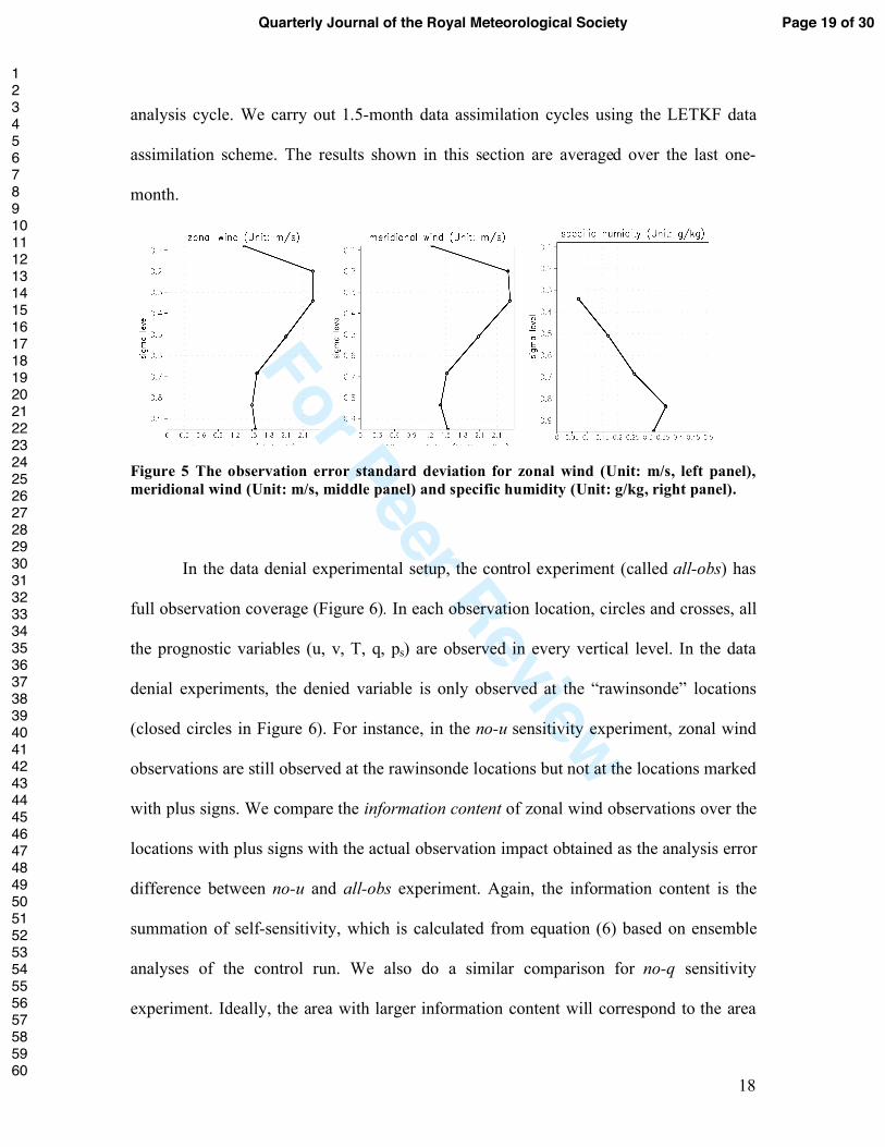
Figure 5 The observation error standard deviation for zonal wind (Unit: m/s, left panel),
meridional wind (Unit: m/s, middle panel) and specific humidity (Unit: g/kg, right panel).
In the data denial experimental setup, the control experiment (called all-obs) has
full observation coverage (Figure 6). In each observation location, circles and crosses, all
the prognostic variables (u, v, T, q, ps) are observed in every vertical level. In the data
denial experiments, the denied variable is only observed at the “rawinsonde” locations
(closed circles in Figure 6). For instance, in the no-u sensitivity experiment, zonal wind
observations are still observed at the rawinsonde locations but not at the locations marked
with plus signs. We compare the information content of zonal wind observations over the
locations with plus signs with the actual observation impact obtained as the analysis error
difference between no-u and all-obs experiment. Again, the information content is the
summation of self-sensitivity, which is calculated from equation (6) based on ensemble
analyses of the control run. We also do a similar comparison for no-q sensitivity
experiment. Ideally, the area with larger information content will correspond to the area
Page 19 of 30Quarterly Journal of the Royal Meteorological Society
1
2
3
4
5
6
7
8
9
10
11
12
13
14
15
16
17
18
19
20
21
22
23
24
25
26
27
28
29
30
31
32
33
34
35
36
37
38
39
40
41
42
43
44
45
46
47
48
49
50
51
52
53
54
55
56
57
58
59
60

For Peer R
eview
19
with larger error differences between the much more expensive sensitivity experiment
and the control run.
Figure 6 Full observation distribution (closed dots: rawinsonde observation network; plus
signs: dense observation network), every observation location is at the grid point.
5.2 Results
Figure 7 shows zonal mean zonal wind analysis RMS error difference (contours)
between no-u and all-obs and the information content (shaded) of zonal wind
observations. Here, the information content is the trace of zonal wind self-sensitivity at
the locations with plus signs in each latitude circle (Figure 6), which reflects the
information extracted from these zonal wind observations at that latitude. Quantitatively,
the analysis RMS error difference (contour) between no-u and all-obs experiment is
largest over the tropics, and is smallest over the mid-latitude Northern Hemisphere (NH).
Qualitatively, the information content (shaded area) agrees with this RMS error
difference, showing the largest values over the tropics and smallest values in the mid-
latitude NH. Interestingly, the zonal wind observations have relatively small impact over
the mid-latitude Southern Hemisphere (SH), even though the rawinsonde coverage is
Page 20 of 30 Quarterly Journal of the Royal Meteorological Society
1
2
3
4
5
6
7
8
9
10
11
12
13
14
15
16
17
18
19
20
21
22
23
24
25
26
27
28
29
30
31
32
33
34
35
36
37
38
39
40
41
42
43
44
45
46
47
48
49
50
51
52
53
54
55
56
57
58
59
60

For Peer R
eview
20
sparse over that region. This is because in the no-u experiment the mass fields, such as
temperature and surface pressure, update the winds analysis in the mid-latitude SH
through the error covariance between these variables. The information content basically
reflects this feature, also showing relatively small values over that region.
Figure 8 shows time averaged zonal wind self-sensitivity (filled grid points) at
observation locations with plus signs (Figure 6) and zonal wind RMS error difference
between no-u and control run at the sixth model level. It shows that self-sensitivity has a
larger value between 30ºS and 30ºN, and so does RMS error difference. However, we
should not over interpret this result. For any two single points, the relative magnitude of
self-sensitivity may not reflect the relative magnitude of RMS error difference between
no-u and control run!due to sampling errors. Self-sensitivity can only qualitatively show
the observation impact over some spatial domain. Since the summation of self-sensitivity
and the sensitivity of the analysis with respect to the background at the same observation
location are equal to 1, Figure 8 indicates that analysis state extracts most of the
information from background forecasts, which is consistent with Cardinali et al. (2004).
Page 21 of 30Quarterly Journal of the Royal Meteorological Society
1
2
3
4
5
6
7
8
9
10
11
12
13
14
15
16
17
18
19
20
21
22
23
24
25
26
27
28
29
30
31
32
33
34
35
36
37
38
39
40
41
42
43
44
45
46
47
48
49
50
51
52
53
54
55
56
57
58
59
60

For Peer R
eview
21
Figure 7 Zonal wind RMS error difference (contour, unit: m/s) between sensitivity
experiment and control experiment, and zonal wind information content (shaded) over
observation locations with plus sign.
Figure 8 Time averaged zonal wind RMS error difference (contour; unit: m/s) between no-u
and control experiment at the sixth model level and self-sensitivity (filled grid point) of
zonal wind observations at locations with plus signs in Figure 6 at the sixth model level.
The highly spatial temporal variability and nonlinear physical processes related
with humidity make humidity observation impact study a very challenging problem (e.g.,
Langland and Baker, 2004). In spite of these challenges, the spatial distribution of
specific humidity information content is consistent with the specific humidity RMS error
difference between no-q and all-obs experiment (left panel in Figure 9). It is important to
note that the information content of specific humidity observations qualitatively reflects
not only the impact on the humidity analysis field, but also the impact on the other
dynamical variables, such as zonal wind (right panel in Figure 9). This originates from
Page 22 of 30 Quarterly Journal of the Royal Meteorological Society
1
2
3
4
5
6
7
8
9
10
11
12
13
14
15
16
17
18
19
20
21
22
23
24
25
26
27
28
29
30
31
32
33
34
35
36
37
38
39
40
41
42
43
44
45
46
47
48
49
50
51
52
53
54
55
56
57
58
59
60

For Peer R
eview
22
multivariate characteristics in all-obs experiment, in which specific humidity
observations linearly affect winds through the covariance, and this effect is maximized in
the tropical upper troposphere (right panel in Figure 9). This large impact of humidity
observations on wind analyses over high tropical levels is consistent with the multivariate
assimilation of AIRS humidity retrievals in a low resolution NCEP Global Forecast
System (Liu, 2007).
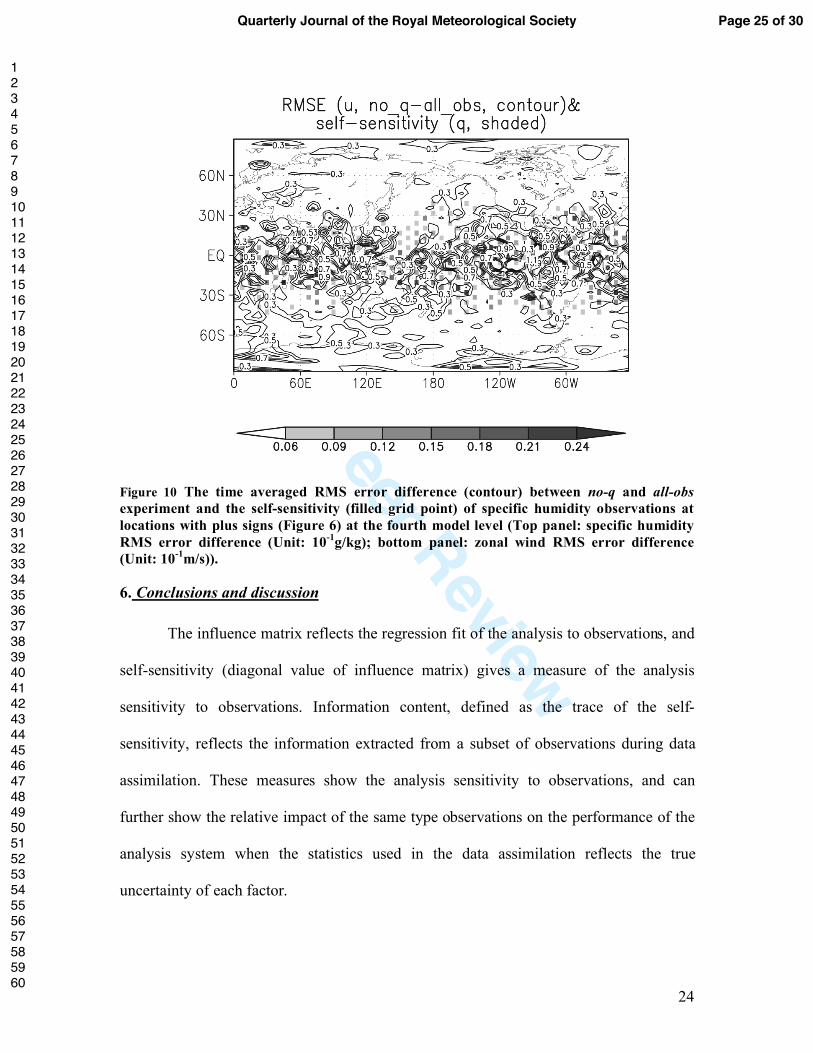
The horizontal distribution of specific humidity self-sensitivity (Figure 10) is also
qualitatively consistent with the analysis RMS error difference between no-q and control
run for both specific humidity and zonal wind. Interestingly, information content and
self-sensitivity of specific humidity observations (Figure 9 and Figure 10) are larger than
those of zonal wind observations (Figure 7 and Figure 8). This means specific humidity
analyses extract more information from humidity observations than zonal wind analyses
extract from zonal wind observations. However, this does not mean that assimilating
specific humidity observations would reduce more error than assimilating zonal wind
observations. This is because specific humidity and zonal wind have different dynamical
roles in the forecast system. The large-scale interaction between zonal wind and the other
dynamical variables during forecast may make zonal wind observations more important
to reduce the overall analysis RMS error. Therefore, information content may not be
applicable to examine the relative impact of observations belonging to different
dynamical variable types on a data assimilation and forecasting system for which forecast
sensitivity to observations may be a more appropriate measure (Langland and Baker,
2004, Liu and Kalnay, 2008). Nevertheless, the qualitative consistency between
information content and the actual observation impact from data denial experiments
Page 23 of 30Quarterly Journal of the Royal Meteorological Society
1
2
3
4
5
6
7
8
9
10
11
12
13
14
15
16
17
18
19
20
21
22
23
24
25
26
27
28
29
30
31
32
33
34
35
36
37
38
39
40
41
42
43
44
45
46
47
48
49
50
51
52
53
54
55
56
57
58
59
60

For Peer R
eview
23
suggests that we can examine the relative impact of the same dynamical variable type
observations in different locations using information content without actually carrying
out much more expensive data denial experiments.
Figure 9 RMS error difference (contour) between no-q and all-obs experiment and specific
humidity information content (shaded) (Left panel: specific humidity RMS error difference
(Unit: 10-1
g/kg); right panel: zonal wind RMS error difference (Unit: m/s)).
Page 24 of 30 Quarterly Journal of the Royal Meteorological Society
1
2
3
4
5
6
7
8
9
10
11
12
13
14
15
16
17
18
19
20
21
22
23
24
25
26
27
28
29
30
31
32
33
34
35
36
37
38
39
40
41
42
43
44
45
46
47
48
49
50
51
52
53
54
55
56
57
58
59
60
For Peer R
eview
24
Figure 10 The time averaged RMS error difference (contour) between no-q and all-obs
experiment and the self-sensitivity (filled grid point) of specific humidity observations at
locations with plus signs (Figure 6) at the fourth model level (Top panel: specific humidity
RMS error difference (Unit: 10-1
g/kg); bottom panel: zonal wind RMS error difference
(Unit: 10-1
m/s)).
6. Conclusions and discussion
The influence matrix reflects the regression fit of the analysis to observations, and
self-sensitivity (diagonal value of influence matrix) gives a measure of the analysis
sensitivity to observations. Information content, defined as the trace of the self-
sensitivity, reflects the information extracted from a subset of observations during data
assimilation. These measures show the analysis sensitivity to observations, and can
further show the relative impact of the same type observations on the performance of the
analysis system when the statistics used in the data assimilation reflects the true
uncertainty of each factor.
Page 25 of 30Quarterly Journal of the Royal Meteorological Society
1
2
3
4
5
6
7
8
9
10
11
12
13
14
15
16
17
18
19
20
21
22
23
24
25
26
27
28
29
30
31
32
33
34
35
36
37
38
39
40
41
42
43
44
45
46
47
48
49
50
51
52
53
54
55
56
57
58
59
60

For Peer R
eview
25
Following the work of Cardinali et al. (2004) within the ECMWF 4D-Var
system, we showed how to calculate self-sensitivity and cross sensitivity (off-diagonal
elements of influence matrix) in the EnKF framework. Based on ensemble analyses
generated in each analysis cycle, the calculation of self-sensitivity and cross-sensitivity in
EnKF only needs the application of the observation operator on each analysis ensemble
member and performing scalar product calculations (equations (6) and (7) in section 2).
By comparing cross-validation (CV) scores calculated from leaving out each observation
in turn and that is based on self-sensitivity, we verified the self-sensitivity calculation and
cross-validation method in EnKF with Lorenz-40 variable model. Unlike the self-
sensitivity calculation in 4D-Var (Cardinali et al., 2004), the self-sensitivity calculated in
EnKF satisfies the theoretical value limits (between 0 and 1) when the observation errors
are not correlated. In agreement with the geometrical interpretation, we showed
experimentally that self-sensitivity is proportional to the analysis errors and anti-
correlated with the observation coverage when the error statistics used in the data
assimilation are fairly accurate.
The squared analysis value change based on analysis sensitivity can be used to
detect observations that produce an unusually large impact on the analysis. This large
impact could be due to large errors in the observations, to the observations being isolated,
or to the atmosphere having a high regional sensitivity to perturbations leading to large
forecast error growth. It would be unfeasible to carry out such computations in its
original formulation even for a model with a moderate number of degrees of freedom.
The computation of the squared analysis value change from leaving out each observation
in turn becomes efficient when using analysis sensitivity in an EnKF but not in the
Page 26 of 30 Quarterly Journal of the Royal Meteorological Society
1
2
3
4
5
6
7
8
9
10
11
12
13
14
15
16
17
18
19
20
21
22
23
24
25
26
27
28
29
30
31
32
33
34
35
36
37
38
39
40
41
42
43
44
45
46
47
48
49
50
51
52
53
54
55
56
57
58
59
60

For Peer R
eview
26
variational formulation because in EnKF no approximations are made in calculating the
sensitivities. We showed that the ability to identify observations that produce unusually
large changes in the analysis can be efficiently used to identify faulty observations during
the analysis cycle, similar to the forecast sensitivity method of Langland and Baker
(2004), Zhu and Gelaro (2008) and Liu and Kalnay (2008).
In an idealized experimental setup, the comparison between information content
and the actual observation impact given by data denial experiments shows qualitative
agreement. This implies that the spatial distribution of information content can be utilized
in examining the relative importance of the same dynamical variable type observations
without actually carrying out much more expensive data denial experiments. However,
information content may not reflect the relative importance of observations from different
dynamical variable types since the relative importance of different dynamical variable
type of observations is also related with the dynamical role they played in the forecast
system. In the future, we will use self-sensitivity and information content to estimate the
importance of the assimilated observations in a more realistic data assimilation system.
Acknowledgements
We are grateful to weather Chaos group in Maryland for suggestions and discussions,
and an anonymous reviewer whose valuable suggestions greatly improved the manuscript.
This work has been supported by NASA grants NNG06GB77G, NNX07AM97G,
NNX08AD40G, and DOE grants DEFG0207ER64437.
Page 27 of 30Quarterly Journal of the Royal Meteorological Society
1
2
3
4
5
6
7
8
9
10
11
12
13
14
15
16
17
18
19
20
21
22
23
24
25
26
27
28
29
30
31
32
33
34
35
36
37
38
39
40
41
42
43
44
45
46
47
48
49
50
51
52
53
54
55
56
57
58
59
60

For Peer R
eview
27
References
Anderson, J. L. (2001), An ensemble adjustment Kalman filter for data assimilation.
Mon. Wea. Rev., 129, 2884-2903.
Anderson, J. L. and S. L. Anderson (1999), A Monte Carlo implementation of the
nonlinear filtering problem to produce ensemble assimilations and forecasts. Mon.
Wea. Rev., 127, 2741–2758.
Bishop, C. H., B. Etherton, and S. J. Majumdar (2001), Adaptive sampling with the
ensemble transform Kalman filter. Part I: Theoretical aspects. Mon. Wea. Rev., 129, 420-
436.
Cardinali, C., S. Pezzulli, and E. Andersson (2004), Influence-matrix diagnostic of a data
assimilation system. Quart. J. Roy. Meteor. Soc. 130, 2767-2786
Desroziers, G., L. Berre, B. Chapnik, and P. Poli (2005), Diagnosis of observation,
background and analysis error statistics in observation space. Quart. J. Roy. Meteor.
Soc., 131, 3385-3396.
Evensen, G. (1994), Sequential data assimilation with a nonlinear quasi-geostrophic model
using Monte Carlo methods to forecast error statistics. J. Geophys. Res., 99 (C5), 10
143-10 162.
Houtekamer, P. L. and H. L. Mitchell (2001), A sequential Ensemble Kalman Filter for
atmospheric data assimilation. Mon. Wea. Rev., 129, 123-137.
Hunt, B. R., E. J., Kostelich, and I., Szunyogh (2007), Efficient Data Assimilation for
Spatiotemporal Chaos: a Local Ensemble Transform Kalman Filter. Physics D., 230,
112-126.
Page 28 of 30 Quarterly Journal of the Royal Meteorological Society
1
2
3
4
5
6
7
8
9
10
11
12
13
14
15
16
17
18
19
20
21
22
23
24
25
26
27
28
29
30
31
32
33
34
35
36
37
38
39
40
41
42
43
44
45
46
47
48
49
50
51
52
53
54
55
56
57
58
59
60
For Peer R
eview
28
Kelly, G., J-N Thepaut, R. Buizza and C. Cardinali (2007), The value of targeted
observations part I : the value of observations taken over the oceans. ECMWF’s
status and plans. ECMWF Tech. Memo., 511, pp27.
Langland, R. H. and Baker, N. L., 2004: Estimation of observation impact using the NRL
atmospheric variational data assimilation adjoint system. Tellus, 56a, 189-201.
Liu, J. (2007), Applications of the LETKF to adaptive observations, analysis sensitivity,
observation impact, and assimilation of Moisture. Ph. D thesis, University of Maryland.
Liu, J. and E. Kalnay, 2008: Estimating observation impact study without adjoint model in
an ensemble Kalman filter. Quart. J. Roy. Meteor. Soc, 134, 1327-1335.
Lord, S. J., E. Kalnay, R. Daley, G. D. Emmit, and R. Atlas: 1997, Using OSSEs in the
design of the future generation of integrated observing system. 1st Symposium on
Integrated Observation Systems, AMS
Lorenz, E. N. and K. A. Emanuel (1998), Optimal sites for supplementary observations:
Simulation with a small model. J. Atmos. Sci., 55, 399-414.
Molteni, F., (2003), Atmospheric simulations using a GCM with simplified physical
parametrizations. I: Model climatology and variability in multi-decadal experiments.
Climate Dyn., 20, 175-191.
Ott, E., B. R. Hunt, I. Szunyogh, A. V. Zimin, E. J. Kostelich, M. Corazza, E. Kalnay,
D. J. Patil, and J. A. Yorke (2004), A Local Ensemble Kalman Filter for Atmospheric
Data Assimilation. Tellus, 56A, 415-428
Rabier, F., N. Fourrie, D. Chafai and P. Prunet (2002), Channel selection method for
Infrared Atmospheric Sounding Interferometer radiances. Quart. J. Roy. Meteor. Soc.
128, 1011-1027.
Page 29 of 30Quarterly Journal of the Royal Meteorological Society
1
2
3
4
5
6
7
8
9
10
11
12
13
14
15
16
17
18
19
20
21
22
23
24
25
26
27
28
29
30
31
32
33
34
35
36
37
38
39
40
41
42
43
44
45
46
47
48
49
50
51
52
53
54
55
56
57
58
59
60

For Peer R
eview
29
Wahba, G. (1990), Spline models for observational data. CMMS-NSF, Regional
conference series in applied mathematics, volume 59. Society for Industrial and
Applied Mathematics.
Whitaker, J. S., and T. M. Hamill (2002), Ensemble data assimilation without perturbed
observations. Mon. Wea. Rev. 130, 1913-1924.
Zhu, Y. and Gelaro, R., 2008: Observation sensitivity calculations using the adjoint of the
Gridpoint Statistical Interpolation (GSI) analysis system. Mon. Wea. Rev. 136,
335-351.
Page 30 of 30 Quarterly Journal of the Royal Meteorological Society
1
2
3
4
5
6
7
8
9
10
11
12
13
14
15
16
17
18
19
20
21
22
23
24
25
26
27
28
29
30
31
32
33
34
35
36
37
38
39
40
41
42
43
44
45
46
47
48
49
50
51
52
53
54
55
56
57
58
59
60