SolarDynamowithSpot

Deposi2on

BidyaBinayKarak,MarkMiesch

AnnaParker,LisaUpton,MausumiDikpa2

JackEddyPostdoctoralresearcher

HighAl2tudeObservatory,NCAR,USA

TheSolarCycle

SolarCycle:Thecyclicvaria2onofthenumberofsunspots.

Image:Wikipedia

BuOerflydiagramofsunspot

La2tudinalposi2onsofsunspotsin2me.

(Mandaletal.2016)

Background

color:theradial

magne2cfieldon

thesolarsurface

  Whyitis11years?

  Whysunspot

propagate

equatorward?

  Whysurfaceradial

fieldpropagate

poleward?Image:D.

Hathaway/

NASA

∂B

∂t= ∇× (V ×B− η∇×B),

ρDv

Dt= −∇p+ ρg + J×B− 2ρΩ0 × v + 2∇.νρS,

Dρ

Dt= −ρ∇.V,

ρTDs

Dt= ∇ · (K∇T )− ρ2Q(T ) + 2ρνS2 +

J2

σ.

Equation of state and proper boundary conditions.

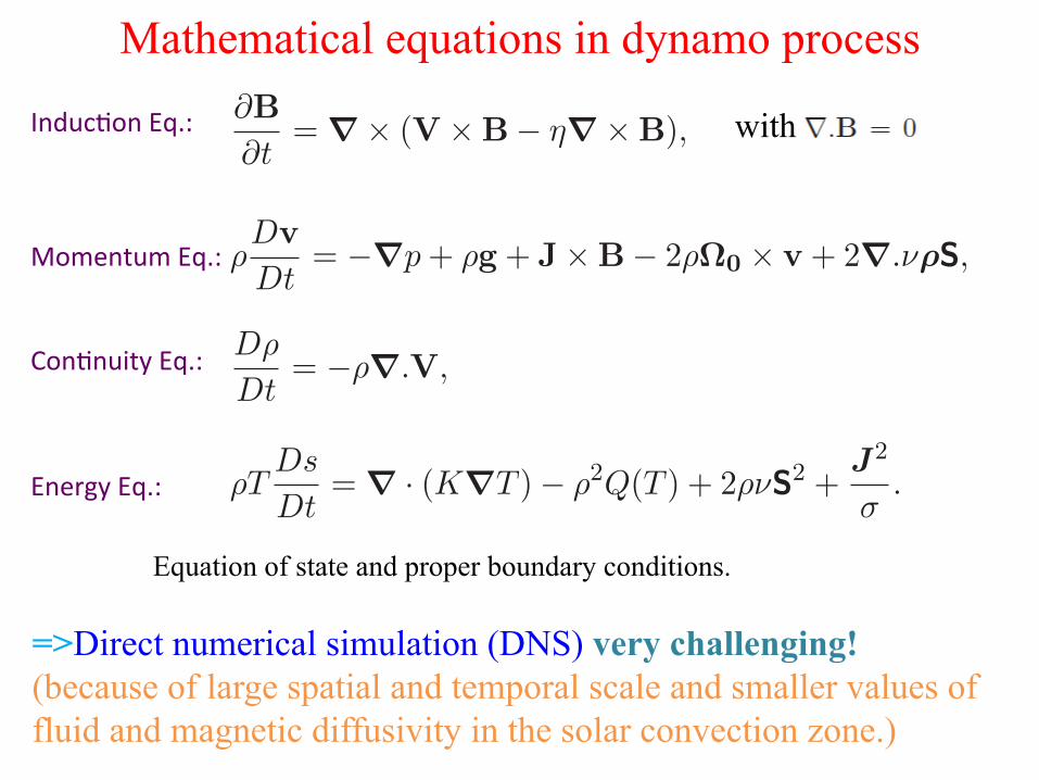
Mathematical equations in dynamo process

with

=>Direct numerical simulation (DNS) very challenging!

(because of large spatial and temporal scale and smaller values of

fluid and magnetic diffusivity in the solar convection zone.)

Induc2onEq.:

MomentumEq.:

Con2nuityEq.:

EnergyEq.:

Results from convection simulations

Karak et al. (2015)

∂B

∂t= ∇× (V ×B− η∇×B),

ρDv

Dt= −∇p+ ρg + J×B− 2ρΩ0 × v + 2∇.νρS,

Dρ

Dt= −ρ∇.V,

ρTDs

Dt= ∇ · (K∇T )− ρ2Q(T ) + 2ρνS2 +

J2

σ.

Kinematic mean-field model

– little easy, but no dynamics!

with

Dynamomodels

Mean-field dynamo model (Parker 1955; Steenbeck, Krause & Raedler 1966)

Mean-field induction equation:

Where

After approximation:

where

Helical alpha effect/

Babcock-Leighton process

Toroidalfield

Poloidalfield

Differen=alrota=on

Large-scale global dynamo: the basic idea

(Parker1955;Steenbeck,Krause&Raedler1966;Babcock1961;Leighton1969)

(Ωeffect)

Poloidal Field Generation: Babcock–Leighton process (Babcock

1961; Leighton 1969; Dasi-Espuig et al. 2010; Kitchatinov & Olemskoy

2011; Munoz-Jaramillo et al. 2012; Priyal et al. 2014; Cameron &

Schussler 2015

Observationally verified!

Equatorward migration of sunspots

Dynamo wave? (Parker–Yoshimura sign rule

1955, 1975; Stix 1976)

Positive alpha and negative

radial shear give equatorward

propagation!

Equatorward migration of sunspots

Dynamo wave? (Parker–Yoshimura sign rule

1955, 1975; Stix 1976)

Positive alpha and negative

radial shear give equatorward

propagation!

poloidal field

generation

Flux transport dynamo

0.89

0

1

v∝Period

(Dikpati & Charbonnea 1999;

Yeates, Nandy & Mackey 2008)

(Wang, Sheeley & Nash 1991; Durney 1995; Choudhuri, Schussler & Dikpati 1995,

and many more)

Mixing length theory ~ 1013 cm2/s

Karak (2010); Karak & Choudhuri

(2010): ~ 1012 cm2/s

Miesch et al (2012):1012 cm2/s

Cameron & Schussler (2016):

3×1012 cm2/s (Simard et al. 2016)

Can quenching help?

(Rudiger, Kitchatinov & Pipin 1994)

Figure from Munoz-Jaramillo et al. (2011)

; Dikpati & Charbonneau 1999

Choudhuri, Schussler & Dikpati 1995

; Hotta & Yokoyama 2010,2011

Challenges in flux transport dynamo

Karak et al. (2014)

Quenching of the diffusivity with B

Measured from convection

simulations --

Confirmed by Simard et al.

(2016) in a more realistic

simulation.

Aaaaaa

aaaaaaa

η

Constructing a high diffusivity

dynamo model

;Dikpa2&Charbonneau1999

Choudhuri,Schussler&Dikpa21995

; Hotta & Yokoyama 2010,2011

2

2

1 1( ) ( ) ( ) ( . )

1( )

r t p

t

Brv B v B B s B

t r r s

rBr r r

θ ηθ

η

∂ ∂ ∂⎡ ⎤+ + = ∇ − + ∇ Ω⎢ ⎥∂ ∂ ∂⎣ ⎦

∂ ∂+

∂ ∂

2

2

1 1( . )( ) ( )t

Av sA A B

t s sη α

∂+ ∇ = ∇ − +

∂

Increased

alpha

coefficient!

=>

Consistent with

αΩ dynamo

wave frequency

(Stix 1976;

Koehler 1973)

For η = 1.5× 1012 cm2/s:

Diffusion time from bottom to

surface ~ 6 years.

So the cycle period must be

less than 6 years!

Densitypumping(duetoagradientinρ),

Turbulentpumping(gradientofvelocity),

Topologicalpumping(topologicalasymmetryoftheflow),

etc.

Pumping of magnetic flux (Droby-shevski&Yuferev1974;Petrovay&Szakaly1993;Brandenburgetal.

1996;Tobiasetal.1998;Tobiasetal.2001;Dorch&Nordlund2001;

Ossendrijver2002;Ziegler&R¨udiger2003;K¨apyl¨aetal.2006;Rogachevskii

etal.2011).

, E = (αB + γ ×B)− ηt∇×B

, E = αB − ηt∇ × B

Turbulent electromotive force in mean-field dynamo

Densitypumping(duetoagradientinρ),

Turbulentpumping(gradientofvelocity),

Topologicalpumping(topologicalasymmetryoftheflow),

etc.

Pumping of magnetic flux (Droby-shevski&Yuferev1974;Petrovay&Szakaly1993;Brandenburgetal.

1996;Tobiasetal.1998;Tobiasetal.2001;Dorch&Nordlund2001;

Ossendrijver2002;Ziegler&R¨udiger2003;K¨apyl¨aetal.2006;Rogachevskii

etal.2011).

, E = (αB + γ ×B)− ηt∇×B

, E = αB − ηt∇ × B

Turbulent electromotive force in mean-field dynamo

Tobias et al. (2001)

Convection simulations:

Pumping speed ~ 1/10th of

convective velocity (Kapyla et al.

2009; Karak et al. 2015;

Warnecke et al 2016...)

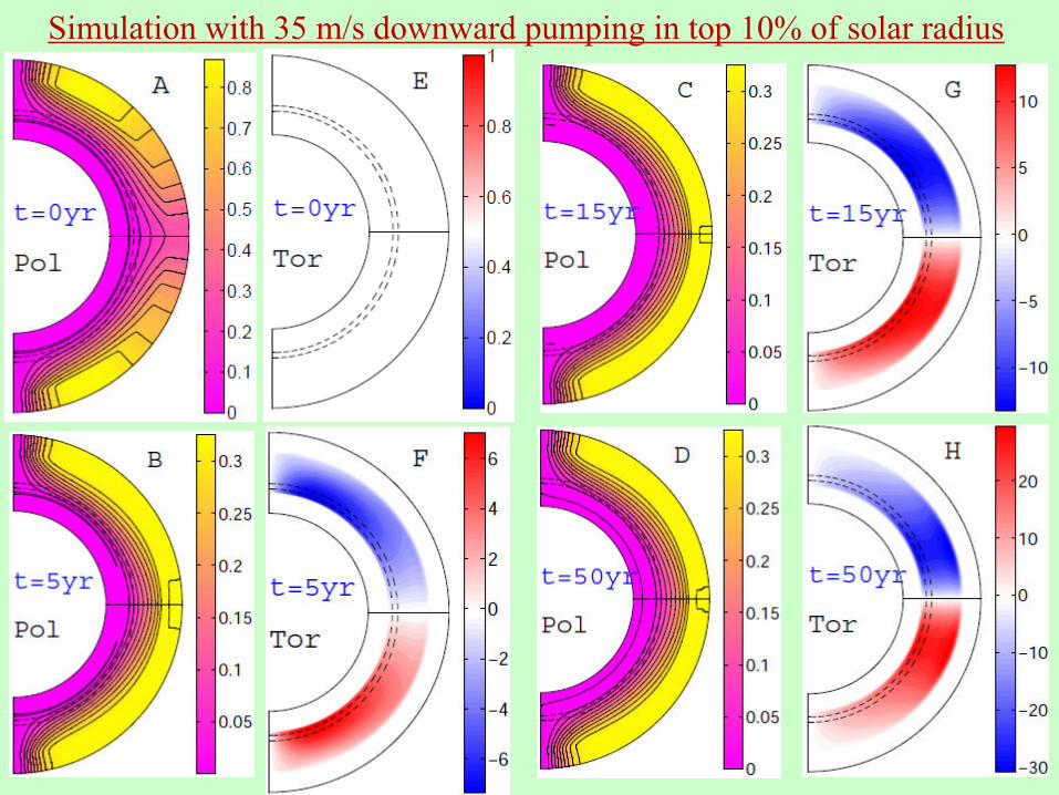
Simulation with 35 m/s downward pumping in top 10% of solar radius

Top: Radial field at surface

Bottom: mean toroidal field over

the whole convection zone.

Equatorward migration is caused by

dynamo wave + flow

Dynamo solution Latitu

de

0 5 10 15 20 25 30 35 40−90

−60

−30

0

30

60

90

−4000

−2000

0

2000

4000

Time (years)

Latitu

de

0 5 10 15 20 25 30 35 40−90

−60

−30

0

30

60

90

−6

−3

0

3

6x 10

4

 Wegivea2lttoeachsunspotgivenbyJoyslaw:(Stenflo&Kosovichov2012;Wangetal.2015)

  Atpresent,themodeliskinema2c

  Diffusivity:2-4×1012cm2/sinthewholeconvec2onzone.

  Inthenear-surfacelayer,wehaveadownwardmagne2cpumpingofabout20m/s.

∂B

∂t= ∇× (v ×B− η∇×B),

3DSolarDynamowithSpotDeposi=on

(a)

v = vr(r, θ)r + vθ(r, θ)θ + r sin θΩ(r, θ)φ,

Dashedline:SOHO/MDIdatafrom

1996-2011.Red/Black:model

δ =32.1

1 + (B/Beq)2cos(θ)

 Weputbipolarspotonthesolarsurfacewithfluxrandomlytakenfromanobservedlog-normaldistribu2on.

  Wedonotputspotateveryintegra2on2mestep!Ratherwetake

itfromalog-normaldistribu2onsuchthatwehavefrequent

erup2onswhenmagne2cfieldisstronger.

Median:

Mean:

  ThisishowwecouplethetoroidalfieldattheboOomofthe

convec2onzonetothefluxinsunspots.

  Wenotethatthe2medelayiscomputedseparatelyineach

hemisphere!

P (∆) =1

σ∆√

2πexp

[

−

(ln∆− µ)2

2σ2

]

DoOedline:SOHO/MDIdata

from1996-2011

Red/Black:dynamomodelmpute r2 ¼ ð2=3Þ lnðssÞ $ lnðspÞ

! "

and l ¼ ln sp þ r2.

τp =1

1 + BenN

B2τ

days,

τs =12

1 + BenN

B2τ

days,

Asteady

dynamo

solu=on

with=lt

angle

quenching

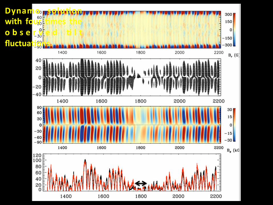
Observedflux

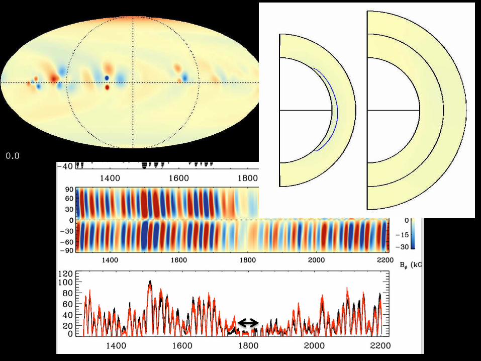
Evolu2onoftheradial

magne2cfieldonthe

surface.

Evolu2onofthemean

toroidalandpoloidal

magne2cfields

Asteady

dynamo

solu=on

with=lt

angle

quenching

Observedflux

Evolu2onoftheradial

magne2cfieldonthe

surface.

Evolu2onofthemean

toroidalandpoloidal

magne2cfields

Dynamo solu=on

with=ltfluctua=ons

cons i s tent w i th

observa=ons!

Dynamo solu=on

with four =mes the

o b s e r v e d = l t

fluctua=ons.Monthlysunspot

number

Dynamo solu=on

with four =mes the

o b s e r v e d = l t

fluctua=ons.

Dynamo solu=on

with four =mes the

o b s e r v e d = l t

fluctua=ons.

Thank you

3. This model is robust under large variations around the

Joy’s law.

Conclusions

1. We are developing a 3D dynamo model, we call it

STABLE (Surface flux Transport and Babcock-

LEighton) dynamo model.

2. This model is driven by the tilted bipolar sunspots

with properties taken from observations.

Thank you

3. This model is robust under large variations around the

Joy’s law.

Conclusions

1. We are developing a 3D dynamo model, we call it

STABLE (Surface flux Transport and Babcock-

LEighton) dynamo model.

2. This model is driven by the tilted bipolar sunspots

with properties taken from observations.