Embed Size (px)
Citation preview
PHYS 705: Classical MechanicsKepler Problem: Geometry of Kepler Orbits
1
Focus-Directrix Formulation
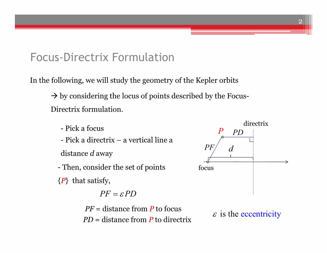
In the following, we will study the geometry of the Kepler orbits
by considering the locus of points described by the Focus-
Directrix formulation.
- Pick a focus
PF PD
focus
directrix
d- Pick a directrix – a vertical line a
distance d away
- Then, consider the set of points
{P} that satisfy,
PD
PF
PF = distance from P to focus
P
PD = distance from P to directrixecce is ntr the icity
2
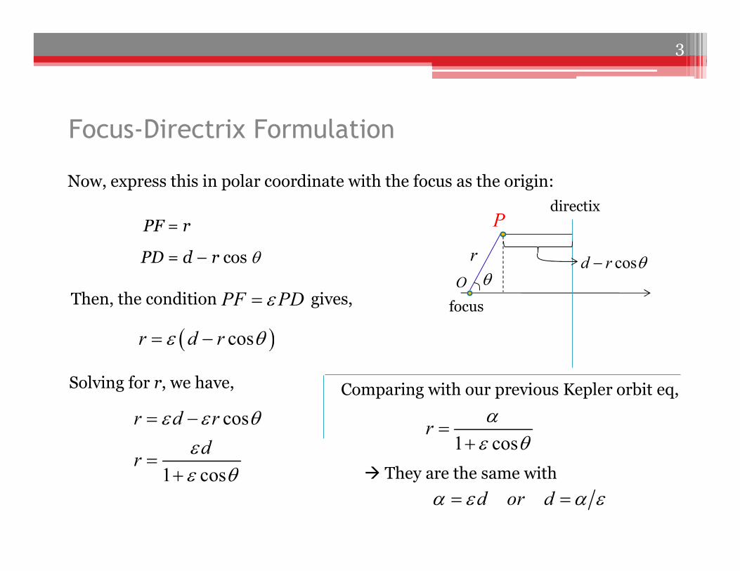
Then, the condition gives,
Focus-Directrix Formulation
Now, express this in polar coordinate with the focus as the origin:
PF PD
PF = r
PD = d – r cos q
focus
directix
cosd r qr
P
qO
cosr d r q
Solving for r, we have,
cos
1 cos
r d r
dr
q q
Comparing with our previous Kepler orbit eq,
1 cosr
q
They are the same with
d or d
3
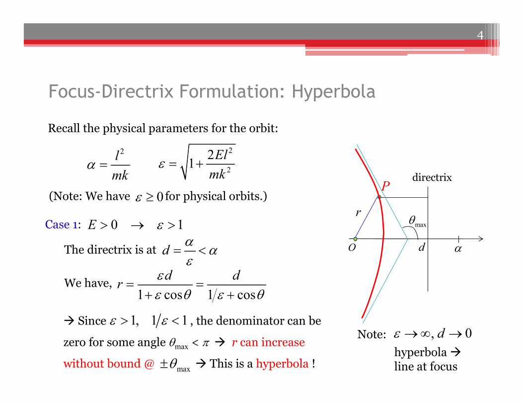
The directrix is at
(Note: We have for physical orbits.)
Focus-Directrix Formulation: Hyperbola
Recall the physical parameters for the orbit:
0
0 1E Case 1:
d
1 cos 1 cos
d dr
q q
2
2
21
El
mk
2l
mk
We have,
Since , the denominator can be
zero for some angle qmax < p r can increase
without bound @ This is a hyperbola !
1, 1 1 , 0d Note:
hyperbola line at focus
directrix
d
r
P
O
maxq
maxq
4
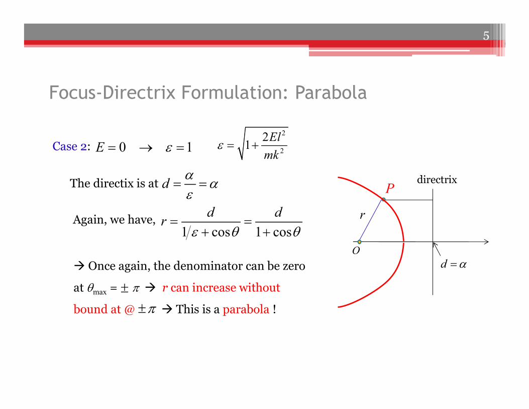
The directix is at
Focus-Directrix Formulation: Parabola
0 1E Case 2:
d
1 cos 1 cos
d dr
q q
Again, we have,
Once again, the denominator can be zero
at qmax = p r can increase without
bound at @ This is a parabola !
p
2
2
21
El
mk
directrix
d
r
P
O
5
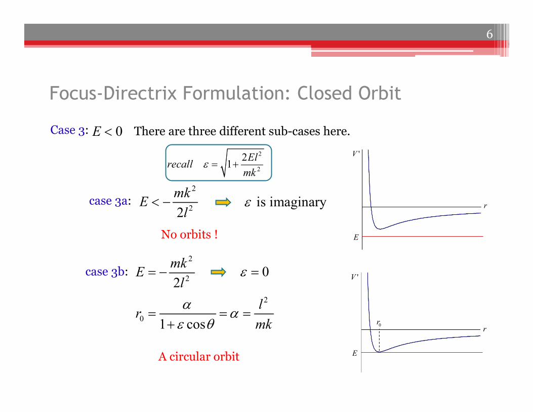
Focus-Directrix Formulation: Closed Orbit
0E Case 3: There are three different sub-cases here.
No orbits !
case 3a: 2
22
mkE
l is imaginary r
E
'V2
2
21
Elrecall
mk
case 3b: 2
22
mkE
l 0
E
'V
r0r
2
0 1 cos
lr
mk
q
A circular orbit
6
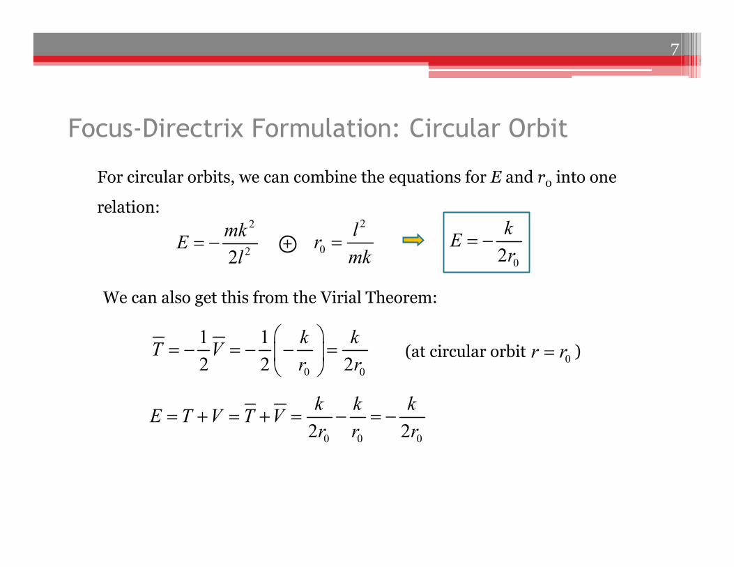
Focus-Directrix Formulation: Circular Orbit
For circular orbits, we can combine the equations for E and r0 into one
relation:2
22
mkE
l
2
0
lr
mk+
02
kE
r
We can also get this from the Virial Theorem:
0 0
1 1
2 2 2
k kT V
r r
0 0 02 2
k k kE T V T V
r r r
(at circular orbit )0r r
7
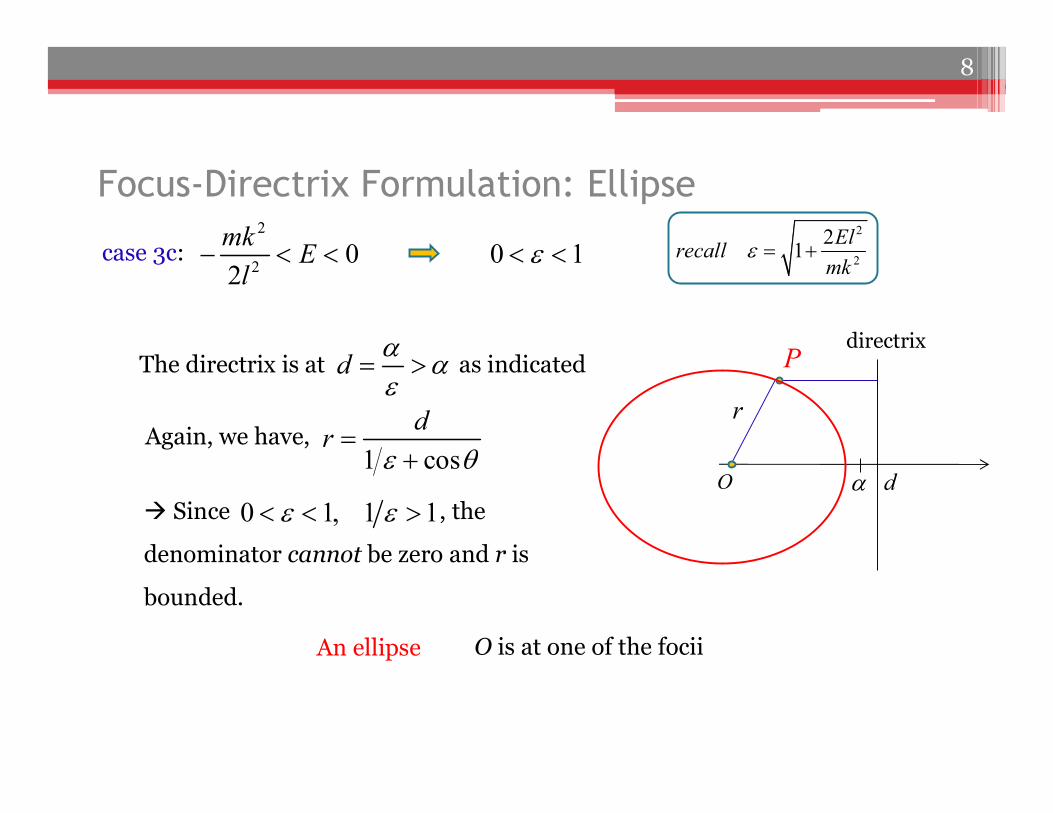
The directrix is at as indicated
Focus-Directrix Formulation: Ellipse
case 3c:
d
1 cos
dr
q
Again, we have,
2
20
2
mkE
l 0 1
Since , the
denominator cannot be zero and r is
bounded.
0 1, 1 1
An ellipse
directrix
d
r
P
O
O is at one of the focii
8
2
2
21
Elrecall
mk
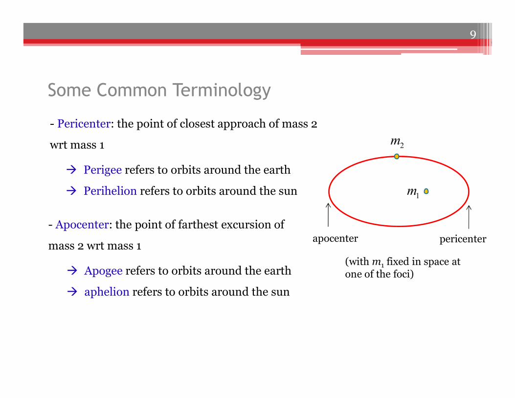
Some Common Terminology
- Pericenter: the point of closest approach of mass 2
wrt mass 1
Perigee refers to orbits around the earth
Perihelion refers to orbits around the sun 1m
2m
pericenterapocenter
(with m1 fixed in space at one of the foci)
- Apocenter: the point of farthest excursion of
mass 2 wrt mass 1
Apogee refers to orbits around the earth
aphelion refers to orbits around the sun
9
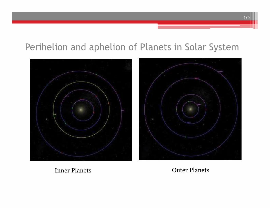
Perihelion and aphelion of Planets in Solar System
Inner Planets Outer Planets
10
O
a
b
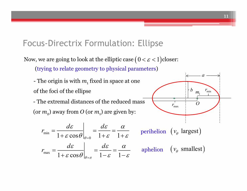
perihelion largestvq
Focus-Directrix Formulation: Ellipse
Now, we are going to look at the elliptic case closer:
- The origin is with m1 fixed in space at one
of the foci of the ellipse
0 1 (trying to relate geometry to physical parameters)
min0
max
1 cos 1 1
1 cos 1 1
d dr
d dr
q
q p
q
q
maxr
minr
- The extremal distances of the reduced mass
(or m2) away from O (or m1) are given by:
aphelion smallestvq
11
1m
Focus-Directrix Formulation: Ellipse
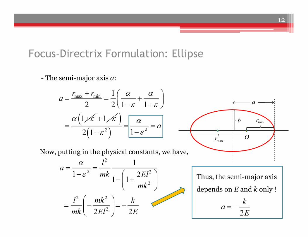
max min 1
2 2 1 1
1
r ra
1 22 12 1
a
O
a
maxr
b minr
- The semi-major axis a:
Now, putting in the physical constants, we have,2
2 2
2
2 2
2
1
1 21 1
2 2
la
mk Elmk
l mk k
mk El E
Thus, the semi-major axis
depends on E and k only !
2
ka
E
12
Focus-Directrix Formulation: Ellipse
22
2
1
2 2
l kE mr
mr r
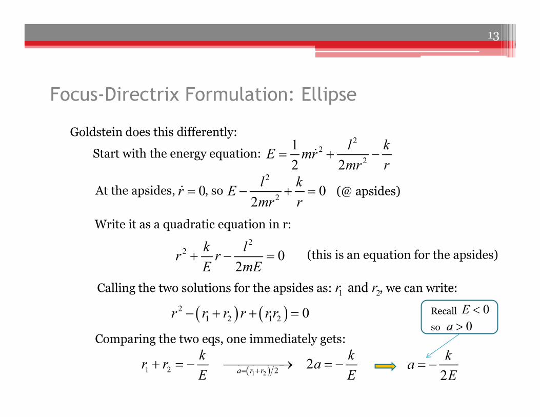
Goldstein does this differently:
At the apsides, , so
2
ka
E
Start with the energy equation:
0r 2
20
2
l kE
mr r (@ apsides)
Write it as a quadratic equation in r: 2
2 02
k lr r
E mE (this is an equation for the apsides)
Calling the two solutions for the apsides as: , we can write:
21 2 1 2 0r r r r r r
1 2 and r r
Comparing the two eqs, one immediately gets:
1 21 2 22
a r r
k kr r a
E E
Recall
so
0E 0a
13
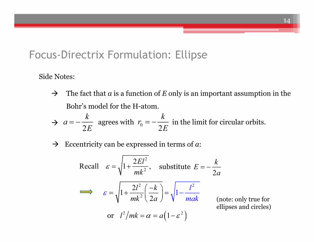
Focus-Directrix Formulation: Ellipse
Side Notes:
Eccentricity can be expressed in terms of a:
2
ka
E agrees with in the limit for circular orbits.
The fact that a is a function of E only is an important assumption in the
Bohr’s model for the H-atom.
substitute2
kE
a
0 2
kr
E
2
2
2Recall 1 ,
El
mk
2
2
2
12
12
l k l
k km a ma
or 2 21l mk a
(note: only true for ellipses and circles)
14
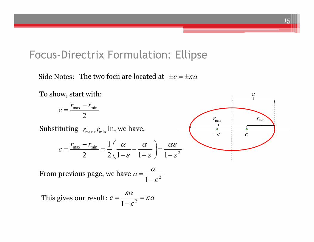
Focus-Directrix Formulation: Ellipse
Side Notes: The two focii are located at c a
max min
2
r rc
From previous page, we have
a
cc
maxr minr
To show, start with:
Substituting in, we have,max min,r r
max min2
1
2 2 1 1 1
r rc
21a
This gives our result: 21c a
15
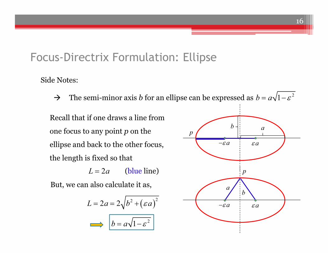
Focus-Directrix Formulation: Ellipse
Side Notes:
The semi-minor axis b for an ellipse can be expressed as 21b a
Recall that if one draws a line from
one focus to any point p on the
ellipse and back to the other focus,
the length is fixed so that
ab
aa
p2L a (blue line)
But, we can also calculate it as,
ab
aa
p
222 2L a b a
21b a
16
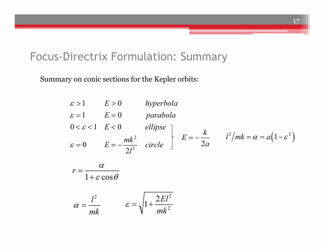
Focus-Directrix Formulation: Summary
Summary on conic sections for the Kepler orbits:
2
2
1 0
1 0
0 1 0
02
E hyperbola
E parabola
E ellipse
mkE circle
l
2
2
21
El
mk
2l
mk
1 cosr
q
2
kE
a
17
2 21l mk a

Focus-Directrix Formulation: Summary
18
Kepler orbits with different energies but with the same angular
momentum
E
l
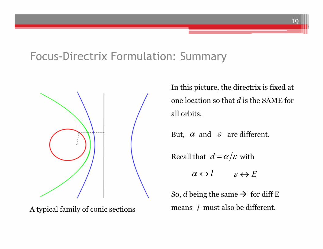
Focus-Directrix Formulation: Summary
19
Recall that with d
l E
So, d being the same for diff E
means must also be different.l
In this picture, the directrix is fixed at
one location so that d is the SAME for
all orbits.
But, and are different.
A typical family of conic sections
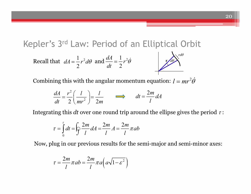
Kepler’s 3rd Law: Period of an Elliptical Orbit
2l mr q
Recall that and r dqrdq
21
2
dAr
dtq 21
2dA r dq
Combining this with the angular momentum equation:
2
22 2
dA r l l
dt mr m
2mdt dA
l
Integrating this dt over one round trip around the ellipse gives the period t :
0
2 2 2m m mdt dA A ab
l l l
t
t p
Now, plug in our previous results for the semi-major and semi-minor axes:
22 21
m mab a a
l lt p p
20
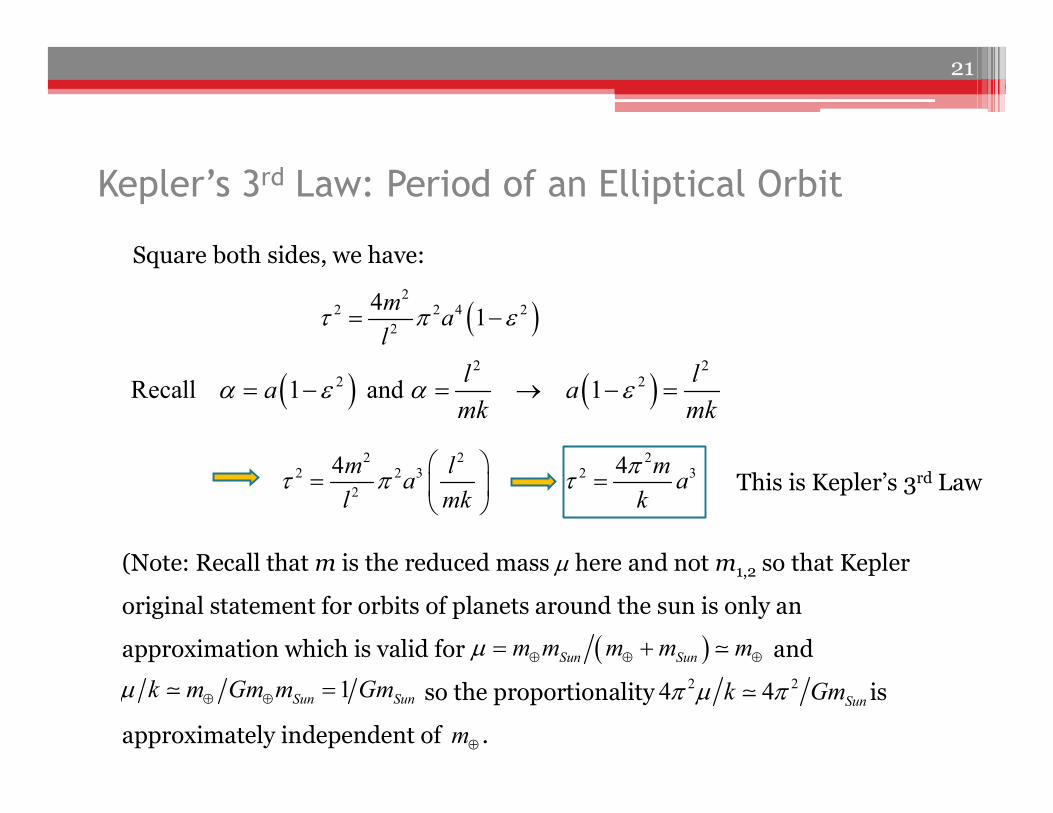
Kepler’s 3rd Law: Period of an Elliptical Orbit
Square both sides, we have:
2
2 2 4 22
41
ma
lt p
2 2
2 2Recall 1 and 1l l
a amk mk
2 2 22 2 3 2 3
2
4 4m l ma a
l mk k
pt p t
(Note: Recall that m is the reduced mass m here and not m1,2 so that Kepler
original statement for orbits of planets around the sun is only an
approximation which is valid for and
so the proportionality is
approximately independent of .
Sun Sunm m m m mm
This is Kepler’s 3rd Law
1Sun Sunk m Gm m Gmm
21
2 24 4 Sunk Gmp m p
m
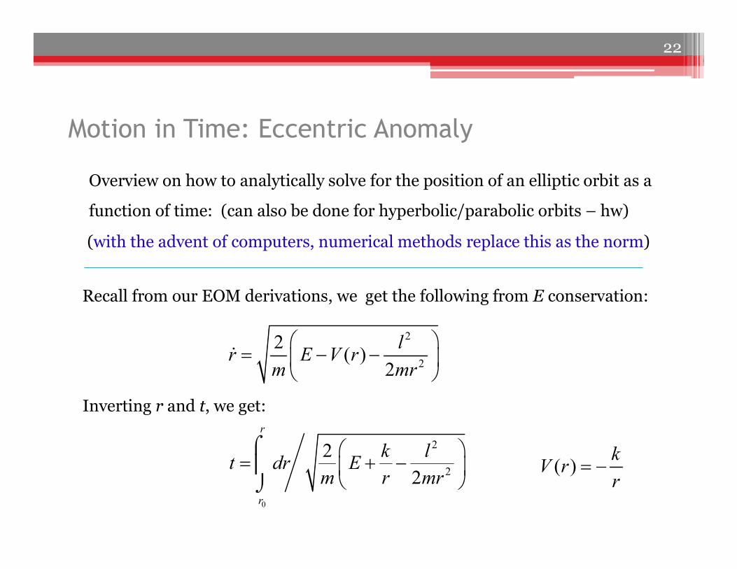
Motion in Time: Eccentric Anomaly
Overview on how to analytically solve for the position of an elliptic orbit as a
function of time: (can also be done for hyperbolic/parabolic orbits – hw)
Recall from our EOM derivations, we get the following from E conservation:
(with the advent of computers, numerical methods replace this as the norm)
2
2
2( )
2
lr E V r
m mr
Inverting r and t, we get:
0
2
2
22
r
r
k lt dr E
m r mr
( )k
V rr
22
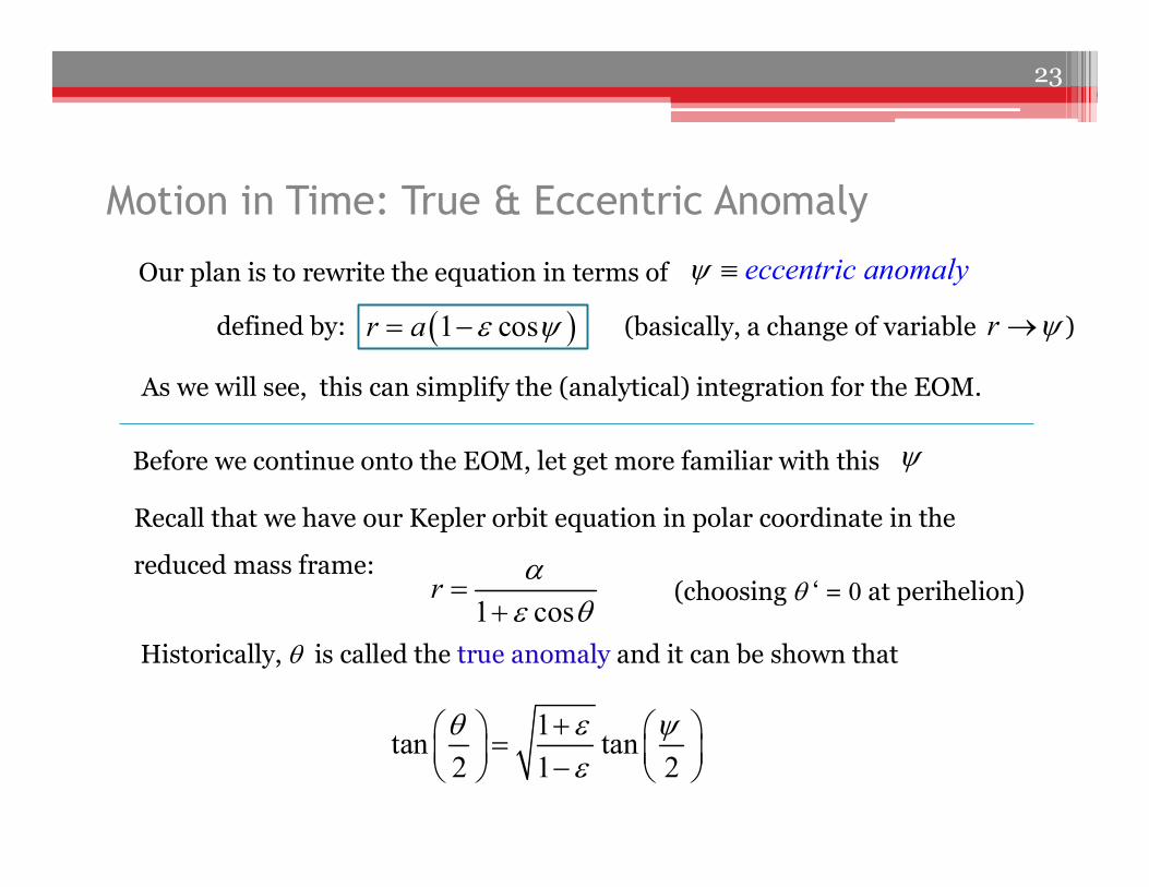
Motion in Time: True & Eccentric Anomaly
Our plan is to rewrite the equation in terms of
defined by: (basically, a change of variable )
eccentric anomaly
1 cosr a r
Before we continue onto the EOM, let get more familiar with this
Recall that we have our Kepler orbit equation in polar coordinate in the
reduced mass frame:
1 cosr
q
Historically, q is called the true anomaly and it can be shown that
1tan tan
2 1 2
q
As we will see, this can simplify the (analytical) integration for the EOM.
(choosing q ‘ = 0 at perihelion)
23
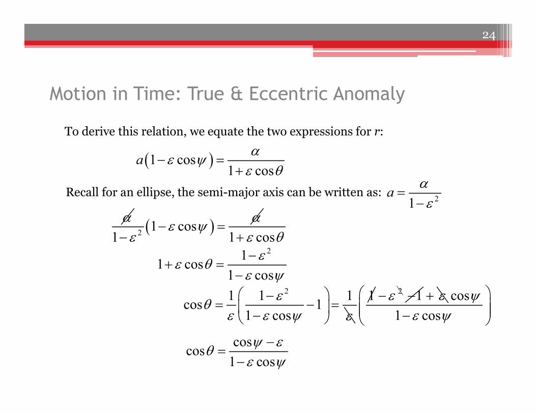
Motion in Time: True & Eccentric Anomaly
To derive this relation, we equate the two expressions for r:
1 cos1 cos
a
q
Recall for an ellipse, the semi-major axis can be written as:
21a
21 cos
1
1 cos q
211 cos
1 cos
q
21 1 1cos 1
1 cos
q
1 2 1 cos
1 cos
coscos
1 cos
q
24
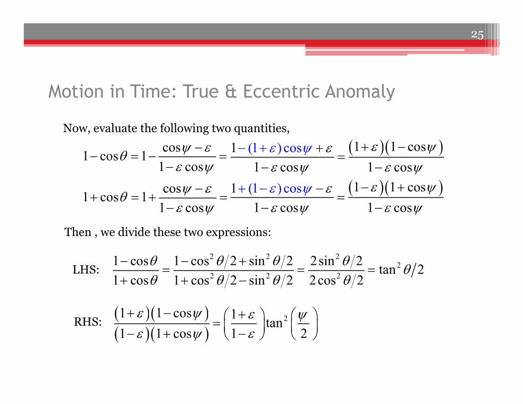
Motion in Time: True & Eccentric Anomaly
Now, evaluate the following two quantities,
cos 11 cos 1
1 co
cos co
os
s
s 1 c
q
cos 11 cos 1
1 co
cos co
os
s
s 1 c
q
Then , we divide these two expressions:
LHS:2 2 2
22 2 2
1 cos 1 cos 2 sin 2 2sin 2tan 2
1 cos 1 cos 2 sin 2 2cos 2
q q q q qq q q q
RHS:
21 1 cos 1tan
1 1 cos 1 2
25
1 1 cos1
1 cos 1
(1 s
c s
) co
o
1 1 cos1
1 cos 1
(1 s
c s
) co
o
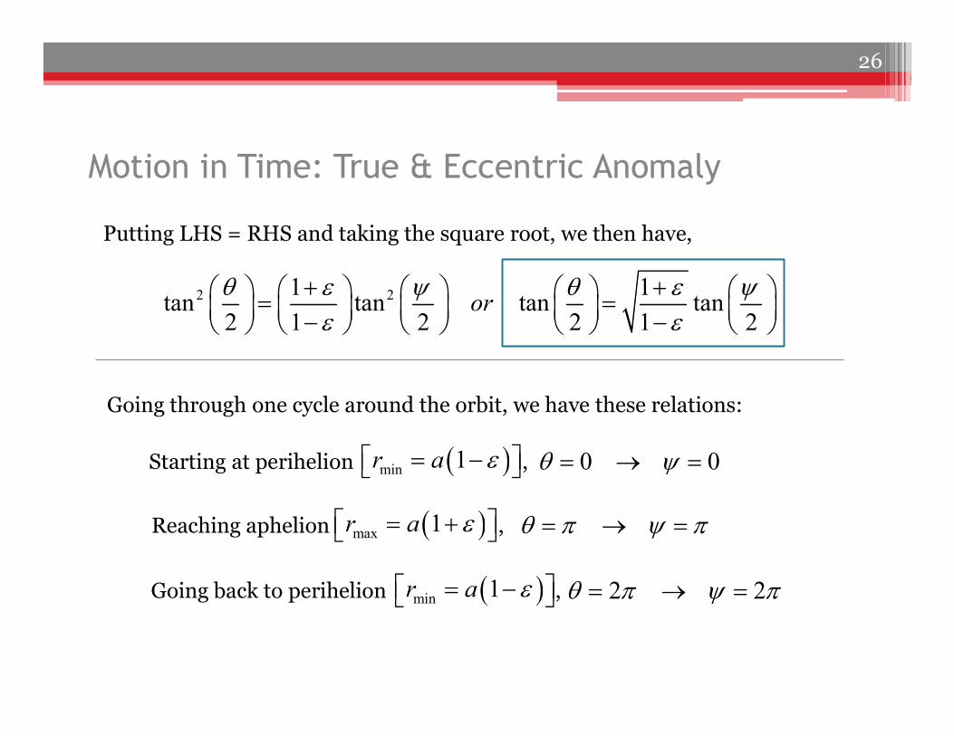
Motion in Time: True & Eccentric Anomaly
Putting LHS = RHS and taking the square root, we then have,
2 21 1tan tan tan tan
2 1 2 2 1 2or
q q
Starting at perihelion , 0 0q min 1r a
Reaching aphelion , q p p max 1r a
Going back to perihelion , 2 2q p p min 1r a
Going through one cycle around the orbit, we have these relations:
26
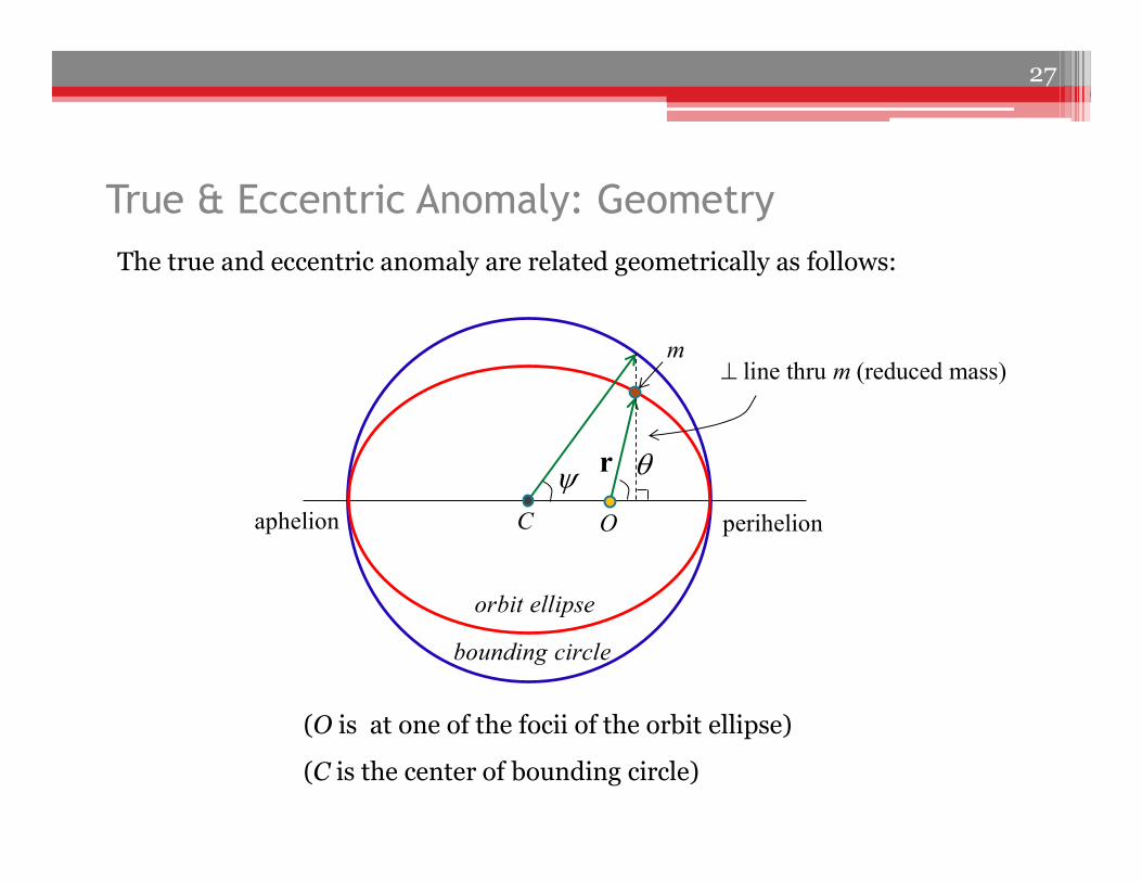
True & Eccentric Anomaly: Geometry
qr
The true and eccentric anomaly are related geometrically as follows:
OC
m
orbit ellipse
bounding circle
line thru (reduced mass)m
perihelionaphelion
(O is at one of the focii of the orbit ellipse)
(C is the center of bounding circle)
27
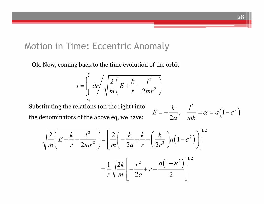
Motion in Time: Eccentric Anomaly
Ok. Now, coming back to the time evolution of the orbit:
Substituting the relations (on the right) into
the denominators of the above eq, we have:
0
2
2
22
r
r
k lt dr E
m r mr
2
2, 12
k lE a
a mk
1/22
22 2
2 21
2 2 2
k l k k kE a
m r mr m a r r
1/222 11 2
2 2
ak rr
r m a
28
Motion in Time: Eccentric Anomaly
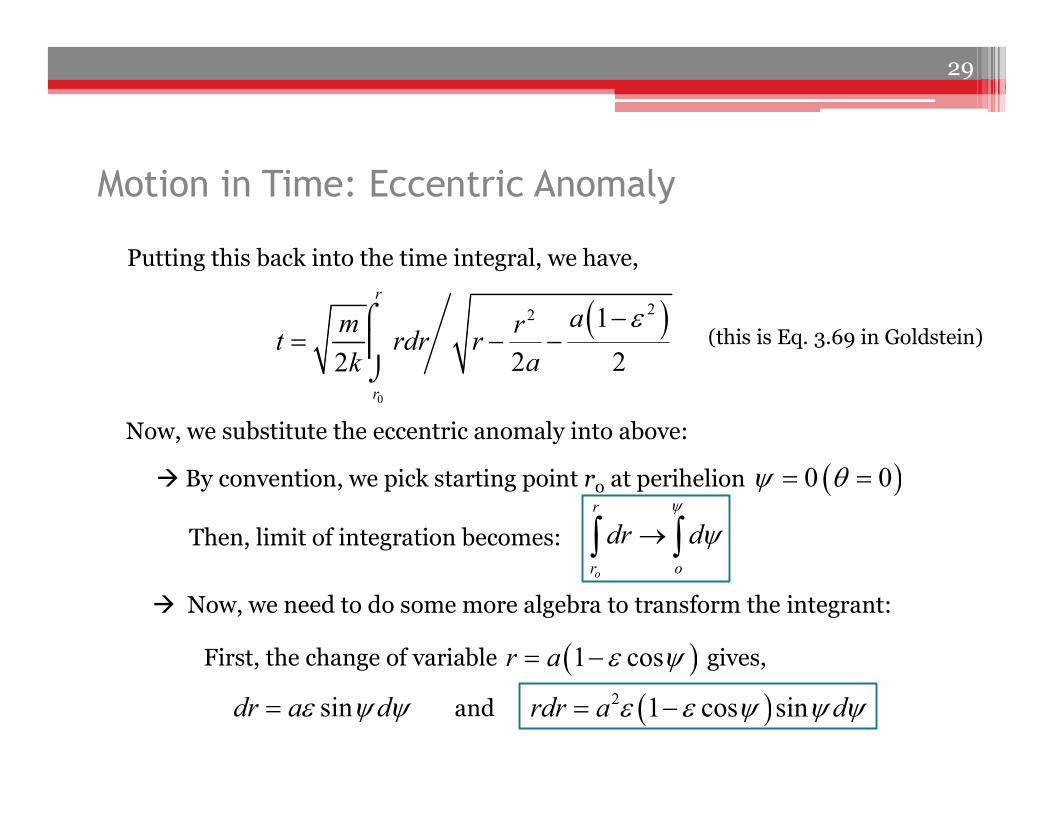
Putting this back into the time integral, we have,
(this is Eq. 3.69 in Goldstein)
0
22 1
2 22
r
r
am rt rdr r
ak
Now, we substitute the eccentric anomaly into above:
By convention, we pick starting point r0 at perihelion 0 0 q
Then, limit of integration becomes:o
r
r o
dr d
Now, we need to do some more algebra to transform the integrant:
First, the change of variable gives, 1 cosr a
sindr a d and 2 1 cos sinrdr a d
29
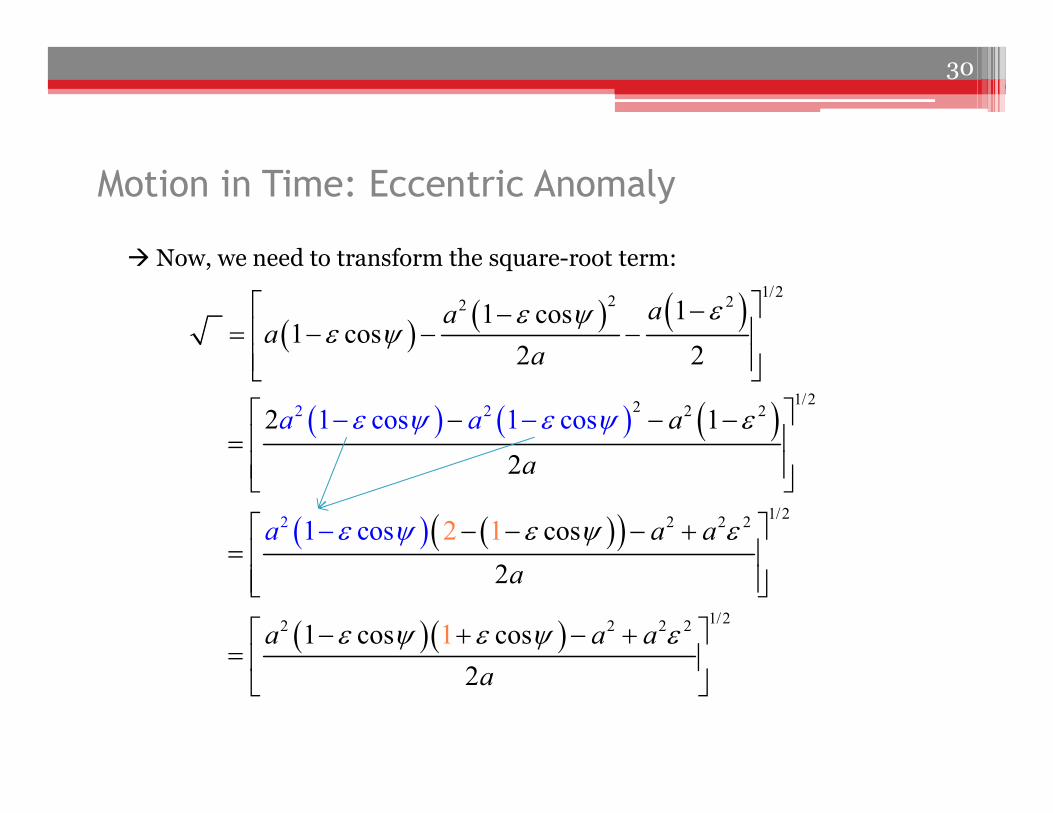
Motion in Time: Eccentric Anomaly
Now, we need to transform the square-root term:
2 21/22 2 2
1/22 2 2
1/22 2 2
2
2
2 1
2
cos
1 cos
2
1 cos cos
2
1 cos
1 c 1
1
os 2
a
a
a a
a
a a a
a
a a
a
30
22 1
2 2
arr
a
1/2
2 22 11 cos1 cos
2 2
aaa
a

0
22
2 2
r
r
am rdr mt
k k a
1 cos ' sin ' 'd sin '
0
3
0
1 cos ' 'ma
t dk
Motion in Time: Eccentric Anomaly
Now, putting all the pieces back together, we have,
2 1a
2 2 2cos a 1/2
2 2
2
a
a
1/2
2 2
2
1 cos2
sin sin2 2
a
a a
2 1 cos sinrdr a d
Recall,
31
Motion in Time: Eccentric Anomaly
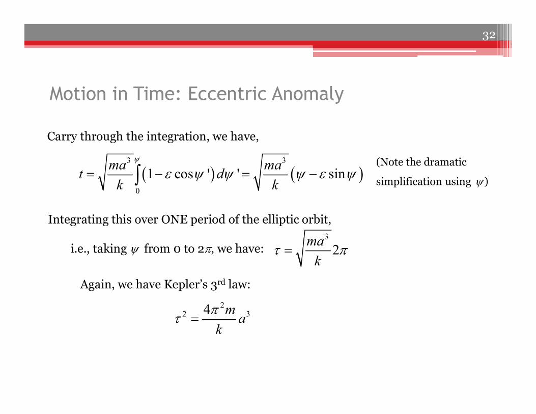
Carry through the integration, we have,
i.e., taking from 0 to 2p, we have:
Again, we have Kepler’s 3rd law:
22 34 m
ak
pt
3 3
0
1 cos ' ' sinma ma
t dk k
(Note the dramatic
simplification using )
Integrating this over ONE period of the elliptic orbit, 3
2ma
kt p
32
2t
M pt
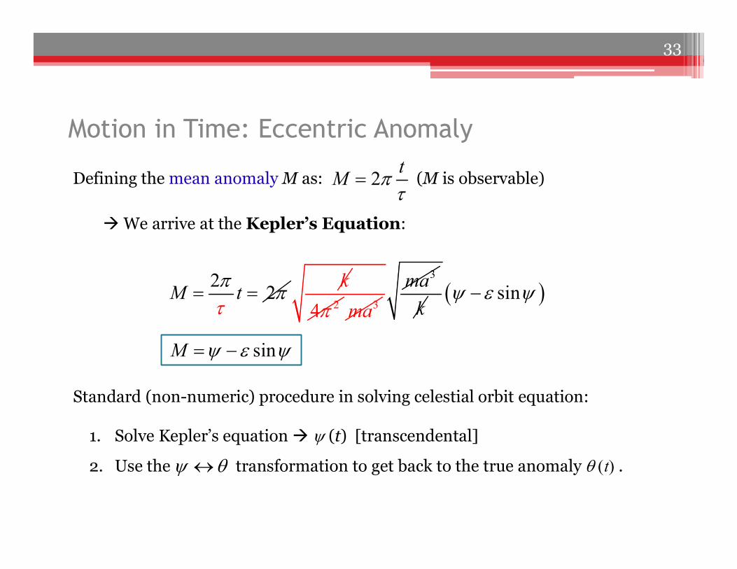
Motion in Time: Eccentric Anomaly
Defining the mean anomaly M as: (M is observable)
We arrive at the Kepler’s Equation:
22M t
tp p
k24p 3ma
3ma
k sin
Standard (non-numeric) procedure in solving celestial orbit equation:
1. Solve Kepler’s equation (t) [transcendental]
2. Use the transformation to get back to the true anomaly q t .
sinM
q
33
• Orbits are heliocentric (orbits with the Sun at the center of force)
e.g. Orbit near Earth Orbit near Mars
• Orbits are on the same orbital plane of the Sun
•
• Ignoring gravitational effects from other Planets
• Thrusts (two) from rockets change only eccentricity and energy of
an orbit BUT not the direction of angular momentum
sun satelliteM m
Hohmann Transfer
The most economical method (minimum total energy expenditure) of
changing among circular orbits in a Kepler system such as the Solar system.
Simplifying assumptions:
34
er
mr
newv
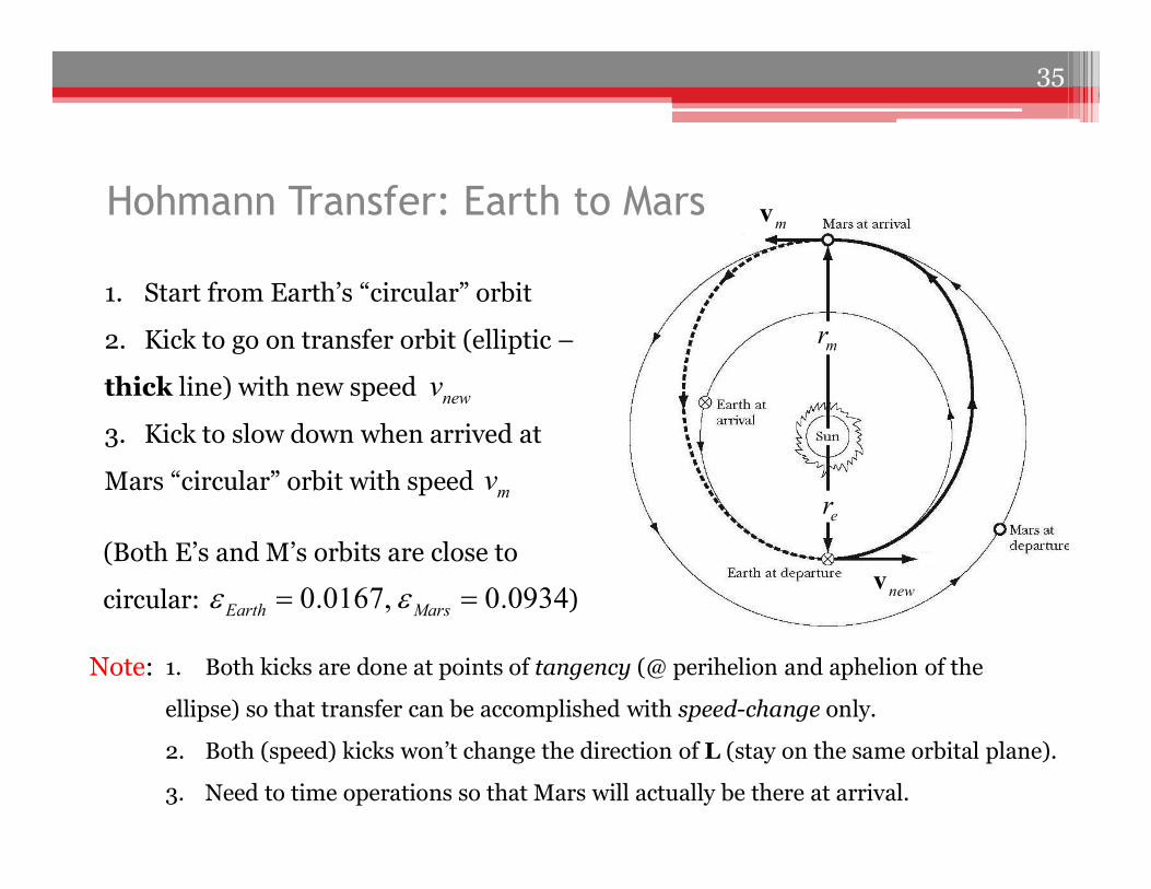
mvHohmann Transfer: Earth to Mars
1. Start from Earth’s “circular” orbit
2. Kick to go on transfer orbit (elliptic –
thick line) with new speed
3. Kick to slow down when arrived at
Mars “circular” orbit with speed
(Both E’s and M’s orbits are close to
circular: )
newv
mv
0.0167, 0.0934Earth Mars
Note: 1. Both kicks are done at points of tangency (@ perihelion and aphelion of the
ellipse) so that transfer can be accomplished with speed-change only.
2. Both (speed) kicks won’t change the direction of L (stay on the same orbital plane).
3. Need to time operations so that Mars will actually be there at arrival.
35
er
mr
newv
mvHohmann Transfer: Earth to Mars
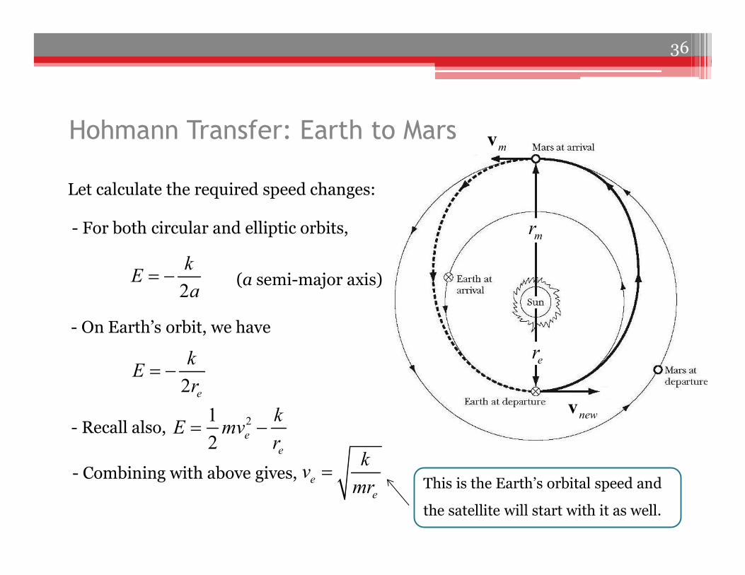
Let calculate the required speed changes:
- For both circular and elliptic orbits,
2
kE
a (a semi-major axis)
- On Earth’s orbit, we have
2 e
kE
r
- Recall also, 21
2 ee
kE mv
r
- Combining with above gives, ee
kv
mr
This is the Earth’s orbital speed and
the satellite will start with it as well.
36
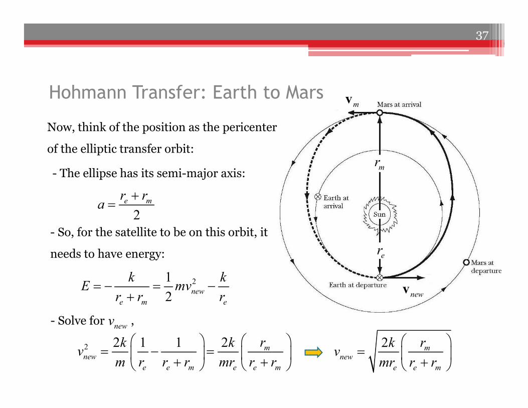
Hohmann Transfer: Earth to Mars
Now, think of the position as the pericenter
of the elliptic transfer orbit:
- The ellipse has its semi-major axis:
2e mr r
a
- So, for the satellite to be on this orbit, it
needs to have energy:
21
2 newe m e
k kE mv
r r r
er
mr
newv
mv
- Solve for ,
2 2 1 1 2 mnew
e e m e e m
rk kv
m r r r mr r r
newv
2 mnew
e e m
rkv
mr r r
37
Hohmann Transfer: Earth to Mars
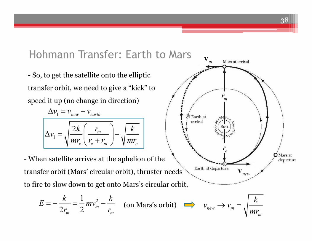
- So, to get the satellite onto the elliptic
transfer orbit, we need to give a “kick” to
speed it up (no change in direction)
er
mr
newv
mv
- When satellite arrives at the aphelion of the
transfer orbit (Mars’ circular orbit), thruster needs
to fire to slow down to get onto Mars’s circular orbit,
1 new earthv v v
21
2 2 mm m
k kE mv
r r (on Mars’s orbit) new m
m
kv v
mr
1
2 m
e e m e
rk kv
mr r r mr
38
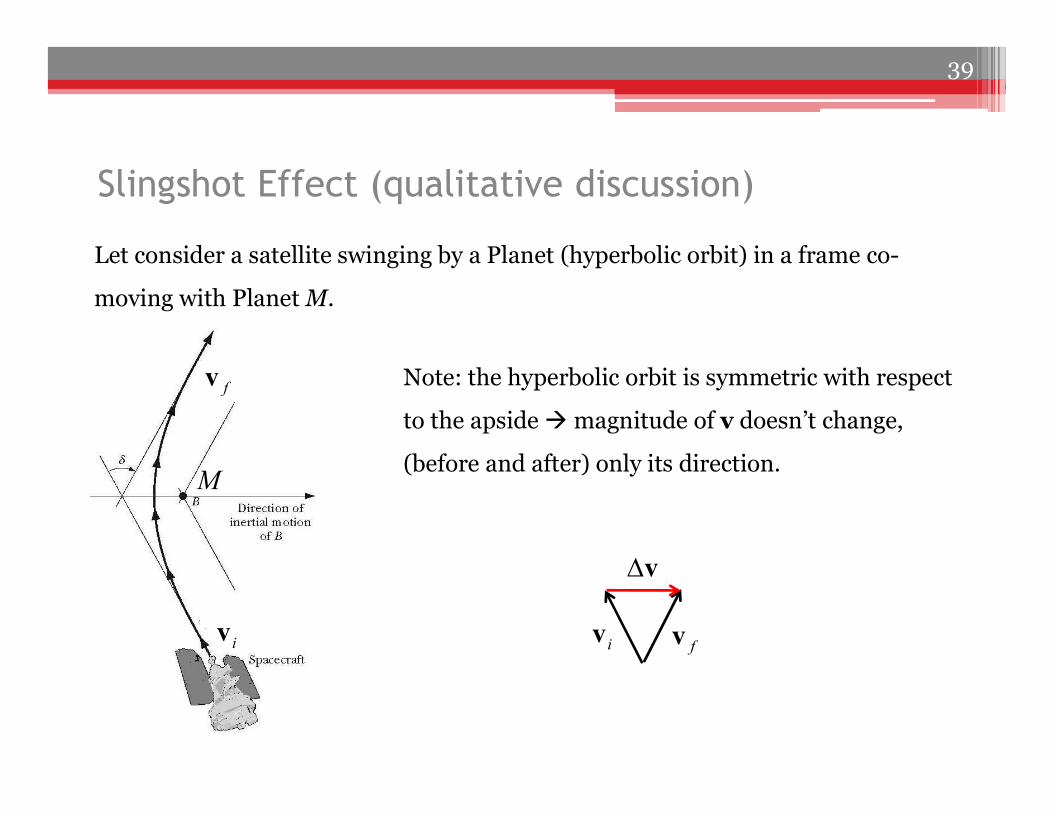
Slingshot Effect (qualitative discussion)
Let consider a satellite swinging by a Planet (hyperbolic orbit) in a frame co-
moving with Planet M.
Note: the hyperbolic orbit is symmetric with respect
to the apside magnitude of v doesn’t change,
(before and after) only its direction.
iv fviv
fv
v
M
39

Slingshot Effect (qualitative discussion)
Now, if we consider the same situation in a “stationary” inertial reference frame
(fixed wrt the Sun) in which the Planet M is moving to the right.
is the velocity of the satellite
in the “stationary” frame. iv
fv
iv
fv 'iv
MvM
'iv
' fv
Mv
is the velocity of the satellite
in the “stationary” frame.
' fv
Note that has a larger magnitude than
(with a boost in the direction of Planet M).
'iv' fv
40
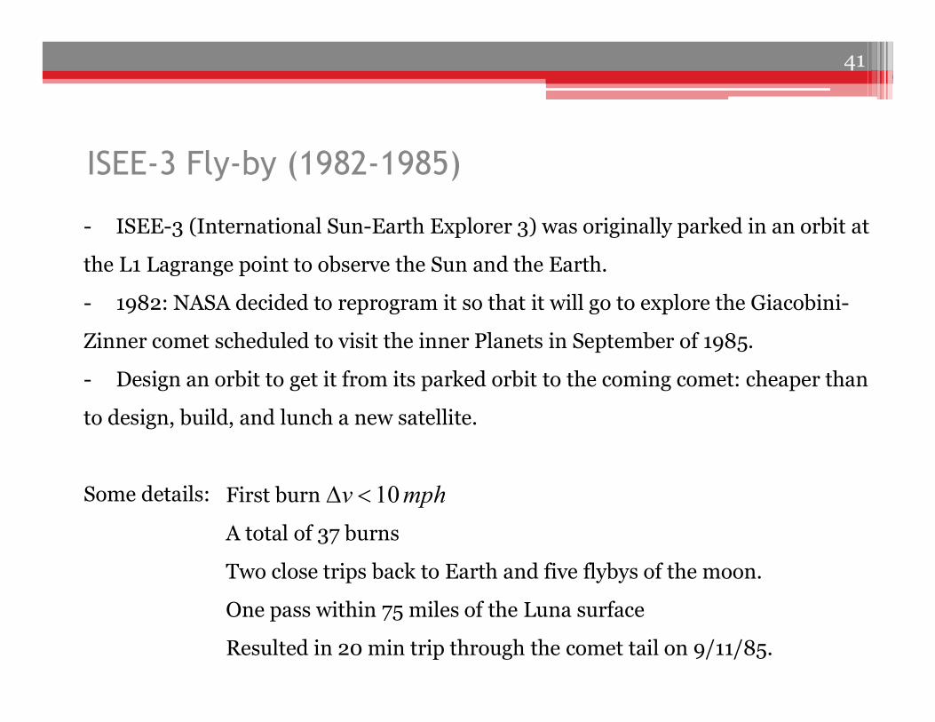
ISEE-3 Fly-by (1982-1985)
- ISEE-3 (International Sun-Earth Explorer 3) was originally parked in an orbit at
the L1 Lagrange point to observe the Sun and the Earth.
- 1982: NASA decided to reprogram it so that it will go to explore the Giacobini-
Zinner comet scheduled to visit the inner Planets in September of 1985.
- Design an orbit to get it from its parked orbit to the coming comet: cheaper than
to design, build, and lunch a new satellite.
Some details: First burn
A total of 37 burns
Two close trips back to Earth and five flybys of the moon.
One pass within 75 miles of the Luna surface
Resulted in 20 min trip through the comet tail on 9/11/85.
10v mph
41
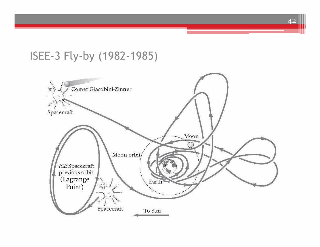
ISEE-3 Fly-by (1982-1985)
(Lagrange Point)
42