Embed Size (px)
Citation preview

!"!#!$!%!&!
!
'()*+,-&.!
!
/!0!1!2!
!
!
3456789:;.<=>?@A FFTB;
!
Design of a Memory-based FFT for Real-Time Heart
Rate Estimation System
!
CDEFGHI!
JKLMFNOP!Q0!
!
!
!
R!S!T! !UV!W!X!Y

3456789:;.<=>?@A FFTB;
!
Design of a Memory-based FFT for Real-Time Heart
Rate Estimation System
!!!!
CDECDECDECDEFFFFGHIGHIGHIGHI!!!!!!!!!!!!!!!!!!!!!!!!!!!!!!!!!!!!!!!!!!!!!!!!!!!!!!!!!!!!!!!!!!!!!!!!!!!!!!!!!!!!!!!!!!!!!!!!!!!!Student FFFFChi-Jen Lan
JKLMJKLMJKLMJKLMFFFFNOPNOPNOPNOP!!!!Q0Q0Q0Q0!!!!!!!!!!!!!!!!!!!!!!!!!!!!!!!!!!!!!!!!!!!!!!!!!!!!!!!!!!!!!!!!!!!!!!!!!!!!!!!!Advisor FFFFDr. Shang-Ho Tsai
"#$%& "#$%& "#$%& "#$%&
'()*+,-&.'()*+,-&.'()*+,-&.'()*+,-&.
/012/012/012/012
A Thesis
Submitted to department of Electrical and Control Engineering
College of Electrical Engineering
National Chiao Tung University
in Partial Fulfillment of the Requirements
for the Degree of
Master of Science
in
Electrical and Control Engineering
May 2011
Hsinchu, Taiwan, Republic of China
R!S!T! !UV!W!!X!Y

3456789:;.<=>?@A FFTB;
CDEFGHI JKLMFNOP Q0
"#$%&'()*+,-&.!
Z[Z[Z[Z[!!!!
\21]^U_45`aAbc'de6789:;.<e>?@Afg
hijklm8'nopqrst'd)u@vwxyz|e~
'34v'emw
89:;.< 89:;.<34¡¢£¤e¥¦§^
¨©¨ vª«;^89¬®¯t67e °m34±² ³´µ¶·!¸¶¹º´»
¼½¾¬Ue¿ÀÁvÂ89:;¥m4 ÃÃÄ Å ÆÃÃÄ
ÇÈ¡¢£¤e;!
ÂÉ@ÇÈ¥m34 óÊË ÌopÍÎ)89:ÏeÐÑÂ]^
e ÃÃÄ ÐÑm²589:;.<U_,ÒÓ9Ôfe.<mÕÖ×4>?
@AeØÙÚÛÜÝ9eÞB;eßàáâãä«åæç Ë蹶·é!
ê³ëìíîÃïðë!ìñòè´ó¶!ÆÆ!óÊË!ôõö÷ø!
!
!
!
!
!
£ùúF>?@A ÃÃÄû8'nû`abcÁ'dûüýû89:;û
óÊË ÇÈ!
!

Design of a Memory-based FFT for Real-Time
Heart Rate Estimation System
StudentFChi-Jen Lan AdvisorFDr. Shang-Ho Tsai
Institute of Electrical and Control Engineering
National Chiao-Tung University
Abstract
This thesis presents a memory-based fast Fourier transform (FFT) for a real time
heart rate estimation system for wearable textile sensors. The electrocardiogram (ECG)
is seriously affected by loose contact between biopotential electrodes and skin, and
body movement. Also, it has baseline wander interference. For the baseline wander
interference, we use the subspace approach to remove the baseline wander component,
then uses the absolute operation for heart rate estimate. The method of heart rate
estimation applies the correlation technique to find the R-R interval and estimates the
heart rate. For the requirement of real time, we use rank one adaptive algorithm to
find dominant eigenvalue by the power method. For the heart rate estimator, we use
FFT and IFFT to achieve the correlation technique.
In the hardware implementation, we use FPGA implementation to achieve the
signal processing and heart rate estimation. In the proposed FFT, we adopt
memory-based architecture to reduce area and power dissipation since heart rate
estimation system is a low frequency system. The resulting design are compiled and
download to the Altera EP2C35F672 Cyclone II FPGA device for real-time
verification.
Keywords: Memory-based FFT, Electrocardiogram, wearable textile
electrodes, baseline wander, heart rate estimation, FPGA
implementation

þÿþÿþÿþÿ!!!!
 !We/0"CDE#R$![%&'ÿeJKLMNOP()
*+,()Â&CD)-.Í/öeLK$!²5()eÔ012eL3$!
J456CD7À7e8¤)¥¦$!9Â\12:;=<m5=>?@«
A8MBe()CöDEFeÿGÂHIJvmKLHIMNOPQLMûR
STLMUVJK«]WXYZ[eG\m3Ö12½]^_`amÂÖEF
b'ÿce=d!
'ÿÇ÷ef"R&gûhij&gûklm&gûnop&gûqrs&
gÂCDâ-RÔ012eJK)tu$'ÿÇ÷eevwtxûmSû
yzU|ÒCDm7~Ç÷eÛ)$UûU
eE$@Ò¬U_CDEe$!²5~eA8
wûm®Â=eCDERm]8ÂCDJvs
tY ¡))ge¢£m¤®Â¥¦7JÔ§¨m©ª«7m
¬~em~e®m©¯°±½²8!
Dm['ÿe³.$n´µe³¶]·¸=¹eº»¼½$
¾8C5CD=ömÕ¬~g¿]eÀÁÂq@Ãm3®Äi`
Å&B$!«ÌÆåU_.EÇÈÉÊeËÌÍÎ'ÿÏ¡ÐÑUÒöe
ÀÁ)wDÓ¯ÿÿmÔÕ£8e)gû³.Ö ¡m×ØÑÙ)
~ÚÛ!
!
!
!
!
!
!
!
!
!
!
!
!
!
!
!
!

Contents
List of Tables iii
List of Figures iv
1 Introduction 1
1.1 Introduction . . . . . . . . . . . . . . . . . . . . . . . . . . . . . . . . . 1
1.2 Literature Survey . . . . . . . . . . . . . . . . . . . . . . . . . . . . . . 2
1.3 Motivation . . . . . . . . . . . . . . . . . . . . . . . . . . . . . . . . . . 4
1.4 Thesis Overview . . . . . . . . . . . . . . . . . . . . . . . . . . . . . . 4
2 Electrocardiogram Background 5
2.1 The Electrocardiogram (ECG) . . . . . . . . . . . . . . . . . . . . . . . 5
2.2 Biopotential Electrodes . . . . . . . . . . . . . . . . . . . . . . . . . . . 8
3 Baseline Wander Removal 11
3.1 Introduction . . . . . . . . . . . . . . . . . . . . . . . . . . . . . . . . . 11
3.2 The Power Method . . . . . . . . . . . . . . . . . . . . . . . . . . . . . 11
3.3 Baseline Wander Removal . . . . . . . . . . . . . . . . . . . . . . . . . 13
3.4 Experiments . . . . . . . . . . . . . . . . . . . . . . . . . . . . . . . . . 14
4 Heart Rate Estimation 16
4.1 Introduction . . . . . . . . . . . . . . . . . . . . . . . . . . . . . . . . . 16
4.2 Correlation Method . . . . . . . . . . . . . . . . . . . . . . . . . . . . . 17
4.3 Experiments . . . . . . . . . . . . . . . . . . . . . . . . . . . . . . . . . 19
i

5 Hardware Implementation 23
5.1 Analog Circuit Design . . . . . . . . . . . . . . . . . . . . . . . . . . . 24
5.1.1 Instrumentation Amplifier . . . . . . . . . . . . . . . . . . . . . 24
5.1.2 Notch Filter . . . . . . . . . . . . . . . . . . . . . . . . . . . . . 25
5.1.3 Lowpass Filter . . . . . . . . . . . . . . . . . . . . . . . . . . . 25
5.1.4 Highpass Filter . . . . . . . . . . . . . . . . . . . . . . . . . . . 26
5.1.5 Output Stage Amplifier . . . . . . . . . . . . . . . . . . . . . . . 27
5.2 Analog-to-Digital Converter . . . . . . . . . . . . . . . . . . . . . . . . 28
5.3 FPGA System . . . . . . . . . . . . . . . . . . . . . . . . . . . . . . . . 30
5.4 Baseline Wander Removal . . . . . . . . . . . . . . . . . . . . . . . . . 32
5.5 Fast Fourier Transform Algorithm . . . . . . . . . . . . . . . . . . . . . 34
5.6 FFT Architecture for Implementation . . . . . . . . . . . . . . . . . . . 39
5.6.1 Memory-based Architecture . . . . . . . . . . . . . . . . . . . . 39
5.6.2 Pipeline Architecture . . . . . . . . . . . . . . . . . . . . . . . . 41
5.7 Heart Rate Estimator . . . . . . . . . . . . . . . . . . . . . . . . . . . . 42
5.8 Experimental and Result . . . . . . . . . . . . . . . . . . . . . . . . . . 50
6 Conclusion and Future Work 52
Bibliography 53
ii

List of Tables
5.1 Pin functions of input . . . . . . . . . . . . . . . . . . . . . . . . . . . . 30
5.2 Pin functions of output . . . . . . . . . . . . . . . . . . . . . . . . . . . 30
iii

List of Figures
1.1 The Filter-bank [14] . . . . . . . . . . . . . . . . . . . . . . . . . . . . 3
2.1 Representative electrical activity from various regions of the heart . . . . 6
2.2 The components of the ECG waveform . . . . . . . . . . . . . . . . . . 7
2.3 The foam-pad electrode . . . . . . . . . . . . . . . . . . . . . . . . . . 9
2.4 The steel textile electrode . . . . . . . . . . . . . . . . . . . . . . . . . 9
3.1 (a) Input signal i(n) (b) The relationship between z(n) and z(n-1) . . . . 13
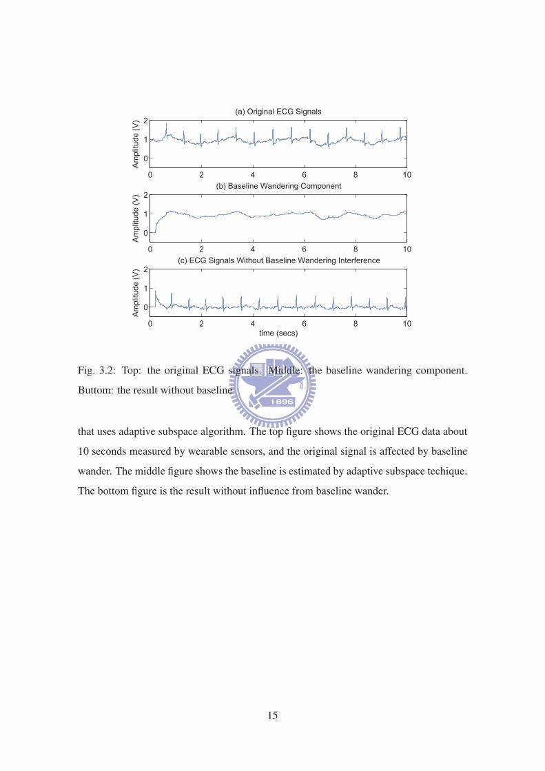
3.2 Top: the original ECG signals. Middle: the baseline wandering compo-
nent. Buttom: the result without baseline . . . . . . . . . . . . . . . . . 15
4.1 Self-correlated . . . . . . . . . . . . . . . . . . . . . . . . . . . . . . . 17
4.2 Correlation values with baseline wander . . . . . . . . . . . . . . . . . . 20
4.3 ECG data in frequency domain . . . . . . . . . . . . . . . . . . . . . . . 21
4.4 Correlation values by FFT and IFFT . . . . . . . . . . . . . . . . . . . . 21
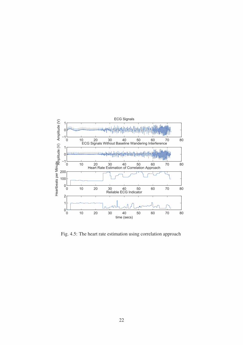
4.5 The heart rate estimation using correlation approach . . . . . . . . . . . 22
5.1 The integral structure of the real time heart rate estimation system . . . . 23
5.2 Basic analog circuits for signal preprocessing . . . . . . . . . . . . . . . 24
5.3 Notch filter . . . . . . . . . . . . . . . . . . . . . . . . . . . . . . . . . 25
5.4 Frequency response of the designed notch filter . . . . . . . . . . . . . . 26
5.5 Second order Sallen-Key lowpass filter . . . . . . . . . . . . . . . . . . . 26
5.6 Frequency response of the designed lowpass filter . . . . . . . . . . . . . 27
5.7 Second order Sallen-Key highpass filter . . . . . . . . . . . . . . . . . . 27
5.8 Frequency response of the designed highpass filter . . . . . . . . . . . . 28
iv

5.9 Output stage amplifier . . . . . . . . . . . . . . . . . . . . . . . . . . . . 28
5.10 Analog-to digital conter, LTC1282 . . . . . . . . . . . . . . . . . . . . . 29
5.11 Timing diagram of LTC1282 . . . . . . . . . . . . . . . . . . . . . . . . 31
5.12 FPGA board . . . . . . . . . . . . . . . . . . . . . . . . . . . . . . . . 32
5.13 Block diagram of baseline wander removal . . . . . . . . . . . . . . . . 33
5.14 Finite state machine of baseline wander removal . . . . . . . . . . . . . 34
5.15 (a) Diagram of 8-point decimation-in-time FFT (b) Decimation-in-time
butterfly . . . . . . . . . . . . . . . . . . . . . . . . . . . . . . . . . . . 36
5.16 (a) Diagram of 8-point decimation-in-frequency FFT (b) Decimation-in-
frequency butterfly . . . . . . . . . . . . . . . . . . . . . . . . . . . . . 37
5.17 (a) Radix-4 decimation-in-frequency butterfly (b) Diagram of 16-point
radix-4 DIF FFT . . . . . . . . . . . . . . . . . . . . . . . . . . . . . . 40
5.18 Block diagram of memory-based architecture . . . . . . . . . . . . . . . 41
5.19 Radix-2 DIF SDF . . . . . . . . . . . . . . . . . . . . . . . . . . . . . . 42
5.20 SDF operation modes (a) mode1 (b) mode2 . . . . . . . . . . . . . . . . 42
5.21 Radix-2 DIF MDC . . . . . . . . . . . . . . . . . . . . . . . . . . . . . 42
5.22 The worst case of situation . . . . . . . . . . . . . . . . . . . . . . . . . 43
5.23 Proposed FFT block diagram . . . . . . . . . . . . . . . . . . . . . . . . 44
5.24 State flow chart of the FFT module . . . . . . . . . . . . . . . . . . . . 44
5.25 Group reverse between input and output . . . . . . . . . . . . . . . . . . 45
5.26 The symmetry property of twiddle factor . . . . . . . . . . . . . . . . . 48
5.27 RAM address assignment of FFT . . . . . . . . . . . . . . . . . . . . . 49
5.28 ROM address assignment of FFT . . . . . . . . . . . . . . . . . . . . . 49
5.29 Brief system specifications . . . . . . . . . . . . . . . . . . . . . . . . . 50
5.30 Compile report of the entire system . . . . . . . . . . . . . . . . . . . . . 51
5.31 Results display on the FPGA device . . . . . . . . . . . . . . . . . . . . 51
v

Chapter 1
Introduction
1.1 Introduction
One of the important physiological signals is electrocardiogram (ECG) that is used to
diagnosing various cardiac diseases such as hypercalcemia and arrhythmia. These dis-
eases is not obvious in initial symptoms. It is used to record the ECG signal for 24 hours
to observe the waveform. However, the ECG medical devices needs more comfortable
electrodes for long-term monitoring. Thus, we focus on wearable textile sensors used in
heart rate estimation system [1]. The wearable textile sensors are comfortable, washable
and durable. However unlike the metal-plate electrodes, textile electrode are dry contact
that affect the ECG signals in measured by respiration, electrodes and body movement.
The heart rate estimation includes the signal processing algorithm and heart rate estima-
tor since the heart rate and the heart rate variability is an important physiological infor-
mation [2]. For the baseline wander induced by texitile electrode, we use the adaptive
subspace algorithm [11] to remove the baseline wander component. Taking the absolute
value for heart rate estimate. In the heart rate estimator, we use fast Fourier transform
(FFT) for computing the correlation value and estimate the heart rate. The results are
emulated by Altera EP2C35F672 Cyclone II FPGA.
1

1.2 Literature Survey
The wearable sensor made of textiles and for the heart rate have been popular recently [3]–
[5]. [3] is tele-home healthcare that uses the wearable medical clothes and bluetooth
receiving terminal for showing and storing the ECG data. Activity patient-monitor [4]
for monitoring belt. The multisensor harness system with acoustic and optical heart rate
sensors, and temperature sensors[5].
In order to reduce the noise from motion artifacts (stading, walking, and running),
many wearable sensors are sewn on clothes or harness [5] to avoid the friction or the
loose contact between electrodes and skin. The ECG data evaluate and disply on terminal
like PC, and use the software like matlab or LabVIEW to estimate the heart rate. Thus,
the distance between system and terminal cannot be too far.
In QRS detection algorithms, almost algorithms use a filter stage to enhance the QRS
complex and attenuate other component since the frequency range of QRS complex is
about 10 to 25 Hz. There are many methods for detecting the QRS complex [12], such as
Derivatives-based, Wavelet-based algorithm, Filter-bank, and Mathematical Morphology
are classic QRS detection algorithms.
The Derivative-based detects the characteristic steep slope of QRS complex [6]. It is
similar to the high-pass filter. The basic Derivative-based algorithm equation is
y1(n) = x(n+ 1)− x(n− 1) (1.1)
The algorithm is simple but it degrades antinoise performance.
The Filter-bank method [14] contains a set of filter to separate the input signal into
various subbands as shown in Fig 1.1. Filter-bank does not affect the time delay and
phase distortions, but it is hard to design a low order, high performance filter.
The Wavelet transform (WT) [7] is used for singularity detection. The WT method
is similar to the Filter-bank that can decompose the ECG signal and enhance the QRS
complex. The coefficient of low-pass and high-pass are approximations and details. We
can design the wavelet filter bank by proper approximations and details coefficients.
The basic operations of Mathematical Morphology [8] are the terms erosion and dila-
2

Fig. 1.1: The Filter-bank [14]
tion, as below
Dilation: f ⊕ g(n) = max(f(n+ i) + g(i)) (1.2)
Erosion: fΘg(n) = min(f(n+ i)− g(i)) (1.3)
Opening: f g(n) = fΘg(⊕g)(n) (1.4)
Closing: f ∗ g(n) = f ⊕ g(Θg)(n) (1.5)
where f(n) is a signal that 1 ≤ n ≤ N and the structure element is g(n) that 1 ≤ n ≤M
and M < N . An erosion followed by a dilation, called Opening. A dilation followed
by an erosion, called Closing. According the opening and closing operation, we can
detect the peak and valley. Thus, it can be used for detecting the QRS complex. The
disadvantage of Mathematical Morphology is mass time requirement.
3

1.3 Motivation
Due to the compaction of life, low exercise, stay up late, and unhealthy habits of eating,
many people are accompanied by chronic illness. The medical device for detecting the
symptoms of disease have been popular. For the convenient and high quality life, a com-
fortable and wearable system is important [3]. The wearable system of ECG monitoring
should be not only comfortable, but also should be have ability of long-term and real-time
monitoring. In order to provide a real-time, small size, and low power ECG monitoring
device, we try to find some ways that can reduce hardware complexity. Therefore we
adopt the memory-based architecture FFT for estimating heart rate.
1.4 Thesis Overview
Chapter 2 reviews the principle of electrocardiogram (ECG) and introduces the proper-
ties of biopotential electrodes. Chapter 3 uses rank one adaptive subspace technique for
removing the baseline wander component and simulation result by matlab. In Chapter 4,
we introduce the heart rate estimator and simulate the heart rate estimation by correlation
technique. In Chapter 5, the FPGA implementation of whole heart rate estimation system
is demonstrated. The last chapter is the conclusion and future work.
4

Chapter 2
Electrocardiogram Background
There are many signals in the body, the bioelectrical phenomena includes electrocardio-
gram (ECG), electromyogram (EMG), and electroencephalogram (EEG), electroneuro-
gram (ENG), and electroretinogram (ERG), They can be converted from energy to the
electrical signals by sensor and there are valuable medical information for symptom of
disease and for diagnosis such as arrhythmia, ventricular hypertrophy, and atriomegaly.
In this thesis, we develop the estimator of heart rate. We introduce the basic of the elec-
trocaridiogram, then discussing why we choose the textile electrodes.
2.1 The Electrocardiogram (ECG)
The electrocardiogram (ECG) signal is produced by heart and the heart is one of the im-
portant organ in the body. ECG records the property of electrical conductivity of the
heart and can be used to detect the heart diseases by analysis the graph. Investigating
the R-R interval can verify the autonomic neuroregulation system. The cycle of ECG
has three phase, the polarization phase, the depolarization phase, and the repolarization
phase. The polarization phase, also called the ready phase that has a resting potential of
approximately -85 mV [9]. During the depolarization phase, the muscle cell has steady
resting potential across the cell membrane, lessening this charge towards zero and leads
to cardiac constriction. The repolarization phase is also called recovery phase and dias-
tole that is between depolarization and polarization. Before the depoalrization phase, it
5

AV NODE
ATRIAL MUSCLE
COMMON BUNDLE
BUNDLE BRANCHES
PURKINJE FIBERS
VENTRICULAR MUSCLE
SA NODE
Fig. 2.1: Representative electrical activity from various regions of the heart
[9]
must returns to polarization, the period between depolarization and polarization is called
repolarization. The action phase in Fig. 2.1 represents the temporal action potential from
each cellular of the heart. The heart has several conductive tissues, such as atrial and
ventricular muscles, sinoatrial(SA) and atrioventricular(AV) nodes, and Purkinje fibers.
Each excitable tissue has its own electrical activity potential. These action potential can
be measure by biopotential electrodes on body interface.
A normal ECG in a period of time, as shown in Fig. 2.2 consist of P, T waves, QRS
complex, PR interval, ST segment and QT interval, described as follows:
• P wave
The P wave is the first upward wave of the ECG and represents left and right atrial
contraction (depolarization). The electrical impulse originate in the sinoatrial (SA)
node and through the atrial musculature. The P wave should be upright and the
duration of P wave should not be more than 0.12 seconds. The atrial problem may
cause abnormal P wave.
6

• QRS complex
The QRS complex is the most important wave in ECG signal. It represents the left
and right ventricular muscles depolarization. The normal duration of QRS com-
plex interval is 0.05 to 0.10 seconds. If the duration is more than 0.12 seconds, it
indicates abnormal intraventricular conduction and ventricular arrhythmia.
Fig. 2.2: The components of the ECG waveform
• T wave
The T wave represents the recovery (repolarization) of the ventricles, usually con-
cerned the direction, the shape, and the height of the wave. The normal direction
of The T wave is upright and the shape is slightly rounded and the normal height is
not above 5 mm. Abnormal T wave may cause dectrolyte disturbance, like hyper-
calcemia and hypocalcemia.
• U wave
7

The U wave is a small additional wave which follows the T wave, it does not always
appear in the ECG. The diabetes, digoxin and slow repolarization of the ventricular
may cause the abnormal tall U wave.
• PR interval
The PR interval is measured from the start of the P wave to the start of the QRS
complex. The duration of the normal PR interval is 0.12 to 0.20 seconds.
• PR segment and ST segment
The PR segment and ST segment are related to isoelectric line. The PR segment
represents the time taken to conduct through the slow AV junction and the ST seg-
ment signifies the period of early deporization of the ventricles.
• QT interval
The QT interval is measured from the start of QRS complex to the end of the T
wave. The interval represents a complete ventricular cycle of depolarization and
repolarization. It should be less than half of the R-R interval. A long QT interval
wider than 1/2 of the R-R interval indicates there is a risk for developing hemody-
namically unstable dysrhythmias and higher incidence of sudden death.
2.2 Biopotential Electrodes
It is necessary to provide some interface between the electronic measuring circuit and the
body for measuring and recording potentials in the body, called biopotential electrodes.
The biopotential electrodes should have the ability of transmitting the current across the
interface between the body and the measuring circuit. The electrode must serve as a
transducer to change an ionic current into an electronic current since current is carried in
the body by ions. There are two types of electrodes, internal (invasive) and body-surface
(noninvasive) electrodes.
• metal-plate electrodes
8

Fig. 2.3: The foam-pad electrode
In recent years, the noninvasive examination has been popular because it’s not need
to hurt or inbreak the body. There are various types of the electrodes such as metal-
plate, suction, floating and flexible electrodes, one of the most frequently used form
of measuring the bioelectric signal is the metal-plate electrodes. Fig. 2.3 is one of
the metal-plate electrodes. This style of the electrode is disk-shaped. When the
electrodes apply to the patient, the area of skin should be clean. we generally use
electrolyte gel which contains Cl− to the patient to maintain good contact. How-
ever, patients’ skin may be over-sensitive with the Ag/AgCl electrodes or uncom-
fortable for long-term monitorting.
• steel textile electrode
Fig. 2.4: The steel textile electrode
In order to increase the comfort of patients’ feeling, the development of fabric-based
electrodes is becoming more important, in this thesis, we measure ECG signals
using textile electrode as shown in Fig. 2.4 to estimate the heart rate in real time.
9

the sensor not only soft and comfortable to the wearing person, but also washable
and reusable for economical consideration.
10

Chapter 3
Baseline Wander Removal
3.1 Introduction
The ECG signals we measured from the body by wearable electrodes of steel textiles have
many interference. The interference is primarily produced by the loose contact with skins
of electrodes, respiration, and body movement. These interference are called baseline
wander that can affect the accurate diagnosis of cardiac diseases. However, it is important
to provide a stable signal and clearly ECG signal characteristic for heart rate estimation
and reliable diagnosis. There are many methods to find out how to remove baseline drift
and they have been proposed in twenty years. Usually we use wavelet transform to decom-
pose the signals and eliminate the baseline wander component. In this thesis, we adopt
adaptive subspace baseline wander removal to achieve lower computation; this method
can be realized in a real-time manner. First, we introduce the power method. Then we use
the power method for removing baseline wandering
3.2 The Power Method
The power method [10] is a way for finding eigenvalue that has the largest in absolute
value in matrix A. At first, we suppose matrix A is an n × n diagonalizable that has a
dominant eigenvalue. Then we choose an initial nonzero vector x0 in Rn. The iteration is
described as follows:
11

for :k = 1, 2, · · ·
zk = Axk−1
xk = zk/‖zk‖
λk = [xk]HAxk
end
Assume the eigenvalues of A are λ1, λ2, · · · , λn, and |λ1| > |λ2| ≥ · · · ≥ |λn|. λ1
is called the dominant eigenvalue of A. Let us explain why the power iteration converges
and the initial vector x0 can be approximated to a dominant eigenvector. Let
x0 = c1y1 + c2y2 + · · ·+ cnyn (3.1)
where c1, c2, · · · , cn are scalars, and y1, y2, · · · , yn are n linear independent eigenvectors
in A. Multiplying both sides of (3.1) by Ak, we have
Akx0 = Ak(c1y1 + c2y2 + · · ·+ cnyn)
= c1Aky1 + c2A
ky2 + · · ·+ cnAkyn
= c1λk1y1 + c2λ
k2y2 + · · ·+ cnλ
knyn
= λk1[c1y1 + c2(
λ2
λ1
)ky2 + · · ·+ cn(λn
λ1
)kyn] (3.2)
We assume that |λ1| is lager than other absoluted eigenvalues in, it follows
|λ2
λ1
| < |λ3
λ1
| < · · · < |λn
λ1
| < 1
Therefore
(λi
λ1
)k ≈ 0, 2 ≤ i ≤ n
where k is sufficiently large. Then the power method in (3.2) converges and the approxi-
mation is given by
Akx0 ≈ c1λk1y1 (3.3)
The approximation in (3.3) improves when k increases. Any scalar multiple of y1 is also
a dominant eigenvactor because y1 is a dominant eigenvector. Thus Akx0 converges and
approaches a multiple of the dominant eigenvector of matrix A.
12

3.3 Baseline Wander Removal
We decompose the ECG signal into various subspaces. that is, the ECG signal can be a
linear combination of various subspaces. The baseline wander component is the principle
subspace that spanned by dominant eigenvalue since the baseline wander has the largest
energy in ECG signal. We use the power method for tracking dominant eigenvector.
The adaptive subspace technique that uses subspace of rank one is sufficient to find the
baseline wander component. It is simple but efficient and can be realized easily.
Assume the data correlation matrix Γ(n) is estimated by input vector i(n). Actually,
Γ(n) is a slowy varing matrix of time, and it updates according to the following formula
Γ(n) = αΓ(n− 1) + (1− α)i(n)iT (n) (3.4)
whereα is 0 < α < 1 and is very close to 1; the input vector i(n) = [x(n − N +
1), . . . , x(n−1), x(n)]T is updated by FIFO (first-in, first-out) shown in Fig. 3.1(a). Then
given an initial nonzero vector z(0), and the power iteration is given by
s(n) = Γ(n)z(n− 1) (3.5)
z(n) =s(n)
‖s(n)‖ (3.6)
(a) (b)
Fig. 3.1: (a) Input signal i(n) (b) The relationship between z(n) and z(n-1)
Now we decompose z(n) in another way that one component is spanned by previous
subspace z(n−1) and the other component∆(n), which is a orthogonal subspace shown
13

in Fig. 3.1(b). Then
z(n) = zT (n)z(n− 1)z(n− 1) +∆(n) (3.7)
From (3.5), we know
s(n− 1) = Γ(n− 1)z(n− 2) (3.8)
Substituting (3.4) and (3.7) into (3.5), we obtain
s(n) =[αΓ(n− 1) + (1− α)i(n)iT (n)]z(n− 1)
=αΓ(n− 1)z(n− 1) + (1− α)i(n)iT (n)z(n− 1)
=αs(n− 1)zT (n− 1)z(n− 2)
+ Γ(n− 1)∆(n− 1)
+ (1− α)i(n)iT (n)z(n− 1) (3.9)
We assume ∆(n− 1) approaches 0 and hence z(n− 1)Tz(n− 2) ≈ 1 because the angle
between z(n− 1) and z(n− 2) approaches 0. Then we have
s(n) = αs(n) + (1− α)i(n)iT (n)z(n− 1) (3.10)
Finally, we obtain the dominant eigenvector and obtain the baseline wander component
as
b(n) = iT (n)z(n)z(n) (3.11)
Then we subtract the baseline from the input signal and the output, i.e
y(n) = i(n)− b(n) (3.12)
3.4 Experiments
In this section, we use the ECG data from Ming Young Biomedical Corporation with 8-
bit resolution and sampling rate of 200 samples per second. By experience, the length of
vector is set to be 40 for adaptive subspace approach. The coefficent α is set to be 0.99.
The larger α leads good converge but slower response, and smaller α leads faster response
but the slower convergence. Fig. 3.2 depicts the performance of baseline wander removal
14
0 2 4 6 8 10
0
1
2(a) Original ECG Signals
Am
plit
ude (
V)
0 2 4 6 8 10
0
1
2(b) Baseline Wandering Component
Am
plit
ude (
V)
0 2 4 6 8 10
0
1
2(c) ECG Signals Without Baseline Wandering Interference
time (secs)
Am
plit
ude (
V)
Fig. 3.2: Top: the original ECG signals. Middle: the baseline wandering component.
Buttom: the result without baseline
that uses adaptive subspace algorithm. The top figure shows the original ECG data about
10 seconds measured by wearable sensors, and the original signal is affected by baseline
wander. The middle figure shows the baseline is estimated by adaptive subspace techique.
The bottom figure is the result without influence from baseline wander.
15

Chapter 4
Heart Rate Estimation
4.1 Introduction
A ECG signals with sequence waves PQRST repeats for every single heartbeat. The R
wave of QRS complex is the primary feature of the cycle in ECG. Therefore, the heart
rate is estimated the reciprocal of the R-R interval. Since the R-R interval is not always
constant, the heart rate is the average of heartbeats per unit time in a specific time win-
dow. Many methods of heart rate estimation have been proposed in thirty years [12]. In
general, the method to detect the energy or frequency of QRS complex and search peaks
to estimate heart rate are, for instance, such as wavelet, filter bank, and mathematical
morphology.
The estimation of heart rate base on wavelet is to decompose the signal; small scales
represent the high frequency component, and large scales represent the low frequency
component of the signal. Thus, wavelet transform can work as a band-pass filter by given
a proper scale [13].
The filter-bank approach is similar to the wavelet transform method. The frequency
of QRS complex is about 3-40 Hz, the P and T waves is about 0.5-10 Hz. Then design
the subbands at different scales to find the local maxima and the position [14].
For mathematical morphology method, that uses nonlinear signal processing operators
to enhance the particular shape of the signals by setting operations like Dilation, Erosion,
Opening and Closing [15]. Since the shape of QRS complex has sharp positive and nega-
16

tive peaks, using a peak-valley (PV) extractor can enhance the QRS complex and suppress
the P, T waves and noise. The opening followed by closing of the signal provides one way
for peak-valley extraction.
4.2 Correlation Method
In this section, we use the correlation approach to find the position of local maxima and
evaluate the heart rate directly. Evaluating the correlation value can clearly distinguish
the distance between the first R wave and the second R wave since the characteristic of
ECG signals is periodic with peaks. As the shifted length l = 2τ , the correlation value
is smaller than shifted length l = τ . Therefore, we can search simply to find the first
R-R interval because the correlation value is largest. Fig. 4.1 depicts the self-correlated
Fig. 4.1: Self-correlated
concept for shifted length l, the peaks reflect the R waves and the distance of R-R interval
is τ . If l = 0, it has maximum correlation value. When l = τ , the magnitude of correlation
17

value is secondary, otherwise, the correlation value should be very small. The correlation
method formula is defined as below
c(l) =∑
n
y(n)y(n+ l) (4.1)
The correlation operates similar to linear convolution. If y(n) is a perfectly periodic sig-
nal, the correlation value should have peak when the signal shifts the multiple of the
period. However it needs mass calculation for computing correlation value directly. For-
tunately, we can use the property of the convolution and apply the Fourier Transform to
reduce the computation [20]. It can be shown as follows
C(ejω) =∑
l
c(l)e−jωl
=∑
l
∑
n
y(n)y(n+ l)e−jωl
=∑
l
∑
m
y(−m)y(l −m)e−jωl
=∑
l
(∑
m
y(−m)e−j(−ω)(−m))y(l −m)e−jω(l−m)
= Y (ejω)Y (e−jω)
= Y (ejω)Y ∗(ejω) if y(n) is real
The input signal from baseline wander removal output should be performed the absolute
output values before we compute the correlation value. After removes the baseline wan-
dering component, the signal has both positive and negative values. Thus, if we use the
correlation method, it will minus the peak of the correlation value and may lead to that
the correlation value is not the primary peak anymore, and misguide to evaluate the real
heart rate.
Before the Fast Fourier Transform (FFT) operation, zero padding is needed in time
domain since the original signal is finite length. One of the property of Discrete Fourier
Transform (DFT) is that the multiplication of two sequences in the frequency domain re-
flects the circular convolution in the time domain. Zero padding makes the computation of
18

the circular convolution equal to linear convolution [16]. The procedure of the correlation
approach is as follows
• y(n): Zero padding to the input signals y(n)
• C(ejω): Perform the FFT of y(n)
• Calculate ‖C(ejω)‖2
• c(l): Perform the Inverse FFT of ‖C(ejω)‖2
Therefore, we can simplify the correlation approach by using the FFT and the Inverse
FFT (IFFT). The peak of correlation value occurs when the ECG signals shift length l.
We obtain the R-R interval between the first R wave and the second R wave without
computation. The heart rate per minute is evaluated by the following formula
Heart Rate = 60× Sampling frequency
R-R interval(4.2)
However, the R-R intervals are not always constant and may be influenced by body move-
ment. The peak of the correlation value vanishes when the periodic of ECG signals is
faraway. Therefore, we propose a reliable ECG indicator Q(n) that shows the difference
of the first R-R interval and the second R-R interval. The position of second R-R interval
can be found by searching directly. The Q(n) is given by
Q(n) =position of 2nd peak(n)− position of 1st peak(n)
position of 1st peak(n)(4.3)
4.3 Experiments
We estimate the heart rate every 512 samples, that is, updates the heart rate about one
second since the sample rate is 512 Hz. Before we use correlation method to find the
R-R interval, removing the baseline wander component is needed. The ECG signal with
baseline wander component shows in Fig. 4.2(a). Fig. 4.2(b) shows the correlation value
of Fig. 4.2(a). Since the correlation value is the product and summation of each point, the
baseline wander component primarily decides the correlation value. Fig. 4.3(b) shows
the frequency domain of Fig. 4.3(a). When the ECG signal transfor to the frequency
19

0 500 1000 1500 2000 2500 3000 3500 4000 4500−1
0
1
2(a) ECG Data with Zero padding
Samples
Am
plit
ude (
V)
0 500 1000 1500 2000 2500 3000 3500 4000 4500−1
0
1
2x 10
4 (b) Correlation value
Shift Length of Samples
Fig. 4.2: Correlation values with baseline wander
domain, we can not find out the information about the R-R interval in frequency domain.
Therefore, we have to perform the IFFT to the time domain.
Fig. 4.4 depicts the result of the correlation approach. The top figure in Fig. 4.4 is the
input of the FFT without baseline wandering component. The bottom figure shows the
result of the correlation method. The ECG data is kept the same as that in section 3.4.
The peak of the correlation values occurs at shift length 181 samples by direct search-
ing, then the heart rate per minute is estimated by previous formula 60 × 200181
= 66.3 per
minute. Fig. 4.5 shows the original ECG data, the ECG signals without baseline wander-
ing component, the heart rate estimate, and the reliable ECG indicator. The ECG data of
a wearing person sits at first, then he walks and jogs. The heart rate estimation is correct
when the person sits. Afterward, the result has error because the ECG quality degrades.
When wearing person jogging, the reliable ECG indicator degrades by loose the contact
of the electrodes.
20

0 500 1000 1500 2000 2500 3000 3500 4000 4500−0.5
0
0.5
1
1.5(a) ECG Data with Zero padding
Samples
Am
plit
ude (
V)
0 100 200 300 400 500 6000
1
2
3
x 106
X: 92Y: 3.335e+006
(b) Frequency domain of ECG data
Samples
Fig. 4.3: ECG data in frequency domain
0 500 1000 1500 2000 2500 3000 3500 40000
0.5
1
1.5(a) ECG Data with Zero padding
Samples
Am
plit
ud
e (
V)
0 500 1000 1500 2000 2500 3000 3500 40000
200
400
600
800
X: 181Y: 791.7
(b) Correlation value
Shift Length of Samples
Fig. 4.4: Correlation values by FFT and IFFT
21
0 10 20 30 40 50 60 70 80−1
0
1ECG Signals
Am
plit
ude (
V)
0 10 20 30 40 50 60 70 80−1
0
1ECG Signals Without Baseline Wandering Interference
Am
plit
ud
e (
V)
0 10 20 30 40 50 60 70 800
100
200Heart Rate Estimation of Correlation Approach
He
art
be
ats
pe
r M
inu
te
0 10 20 30 40 50 60 70 800
1
2Reliable ECG Indicator
time (secs)
Fig. 4.5: The heart rate estimation using correlation approach
22

Chapter 5
Hardware Implementation
Fig. 5.1: The integral structure of the real time heart rate estimation system
Fig. 5.1 depicts the entire hardware architecture. After receiving the ECG signals
from wearable textile, we filter the power-line interference and the frequency does not
belong to ECG. We need analog front-end circuits (AFE). The circuits also amplify ECG
signals for the A/D converter. After A/D converter, the signals is transmitted to an FPGA
for signal processing and heart rate estimation. Finally The heart rate is displayed on the
seven segment.
23

5.1 Analog Circuit Design
In order to observe and measure the weak signals (about 1mV) from body, amplify the
signal to proper voltage level is needed. Therefore, one of the purpose of analog front-end
circuits is to amplify the weak ECG signal. Then removes the power-line interference 60
Hz and obtain the ECG signal frequency band. Fig. 5.2 shows the entire analog circuits.
Vin+
Vin-
Vout
Instrumentation
Amplifier
Notch
Filter
Lowpass
FilterHighpass
Filter
Noninverting
Amplifier
Fig. 5.2: Basic analog circuits for signal preprocessing
The circuits are worked on 3.3V single supply.
5.1.1 Instrumentation Amplifier
The instrumentation amplifier should provide the high common-mode rejection ratio (CMRR)
and the high input impedance. In general, the instrumentation circuit needs several oper-
24

ational amplifiers. However, we adopt AD623 to achieve that has low noise, high CMRR,
high input impedance, low input bias current and can operate in 3.3V single supply.
5.1.2 Notch Filter
Since ECG signals are easily affected by 60 Hz power-line interference or couple with
noise from surroundings. The notch filter aim to filter 60Hz. We adopt a twin T circuit as
a notch filter is shown in Fig. 5.3. We use MultiSim to confirm the frequency response.
The result is performed in Fig. 5.4.
Fig. 5.3: Notch filter
5.1.3 Lowpass Filter
In order to achieve the bandpass filter, we can combine the lowpass filter and the high
pass filter as a bandpass filter. In lowpass filter circuits, we adopt the Sallen-Key active
filter to realize [17]. Fig. 5.5 shows a generic second order Sallen-Key lowpass filter. The
cutoff frequency can obtain by following equation
fc =1
2π√R1R2C1C2
(5.1)
The simulation result is shown in Fig. 5.6
Fig. 5.6 is the frequency response of lowpass filter that we designed.
25

Fig. 5.4: Frequency response of the designed notch filter
Fig. 5.5: Second order Sallen-Key lowpass filter
5.1.4 Highpass Filter
The highpass filter also use a second order Sallen-Key highpass filter. Fig. 5.7 is the
highpass filter that we designed. The cutoff frequency fc is also computed by (5.1) and
the cutoff frequency set to be 0.2 Hz. The frequency response is shown in Fig. 5.8.
26

Fig. 5.6: Frequency response of the designed lowpass filter
Fig. 5.7: Second order Sallen-Key highpass filter
5.1.5 Output Stage Amplifier
After we filter the frequency of interference, it is necessary to amplify the signals for A/D
converter. We design a noninverting amplifier with a large gain by following equation
Vout = (1 +Rb
Ra
)Vin + Vbias (5.2)
The Ra and Rb is chosen 1 kΩ and 600 kΩ respectively, and the gain achieve to 600
approximately. The amplifier circuits is shown in Fig. 5.9. The bias voltage 1.2V that
27

Fig. 5.8: Frequency response of the designed highpass filter
Fig. 5.9: Output stage amplifier
A/D converter provided without using operation amplifier.
5.2 Analog-to-Digital Converter
Before signal processing and estimates the heart rate on the FPGA, it is necessary to
convert the analog ECG signal without interference to digital. We adopt the analog-to-
digital converter (ADC) LTC1282 that Linear Technology produced. The main features
of LTC1282 are
28

• Single supply 3V or dual supply ±3V.
• 140ksps throughput rate. Resolution is 12-bit.
• Internal synchronized clock.
• 12mW low power consumption.
• 6µs maximum conversion time.
The operation works on 0V to 2.5V conversion range, single supply 3V. Fig. 5.10 shows
the typical application with single supply, and the pin functions is shown in Table. 5.1 and
Table. 5.2
Fig. 5.10: Analog-to digital conter, LTC1282
Since A/D converter has internal clock, it does not need external clock to synchronize
the control line. We can control the conversion by HSBN, CS, RD. These input is pro-
duced by FPGA. First we set HSBN low to enable the slow memory mode. Control CS
and RD low to read analog signal. Therefore. regular low for CS and RD can achieve
the 512Hz sampling frequency. During the conversion status, the BUSY signal from A/D
29

Table 5.1: Pin functions of input
Inputs
AIN Analog input. 0V to 2.5V (Unipolar) ±1.25V (Bipolar)
HSBN High byte enable input.
This pin is used to multiplex the internal 12-bit conversion
result into the lower bit outputs.
CS The Chip Select input must be low for the ADC to recognize
RD and HBEN inputs.
RD Read input. The active low signal starts a conversion when
CS and HSBN are low.
Table 5.2: Pin functions of output
Outputs
VREF +1.2V reference output.
BUSY The BUSY output shows the converter status.
It is low when a conversion is in progress.
D11-D4 Three-State data outputs. D11 is the most significant bit.
D3/11-D0/8 Three-state data outputs.
converter ouput change to low and BUSY return to high when conversion is over. The
result output on pins D11,. . . , D0 in parallel. The timing diagram of the A/D converter is
show in Fig. 5.11
5.3 FPGA System
A Field Programmable Gate Array (FPGA)is a semiconductor device that has programmable
logic element. The logic element can be programmed to achieve the function of basic gate
circuit like NOT, AND, OR and XOR, or some complex function such as mathematical
30
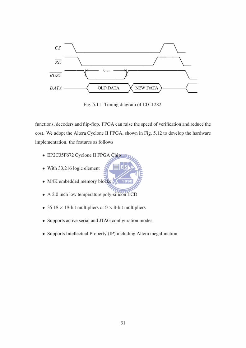
Fig. 5.11: Timing diagram of LTC1282
functions, decoders and flip-flop. FPGA can raise the speed of verification and reduce the
cost. We adopt the Altera Cyclone II FPGA, shown in Fig. 5.12 to develop the hardware
implementation. the features as follows
• EP2C35F672 Cyclone II FPGA Chip
• With 33,216 logic element
• M4K embedded memory blocks
• A 2.0 inch low temperature poly-silicon LCD
• 35 18× 18-bit multipliers or 9× 9-bit multipliers
• Supports active serial and JTAG configuration modes
• Supports Intellectual Property (IP) including Altera megafunction
31

Fig. 5.12: FPGA board
5.4 Baseline Wander Removal
Fig. 5.13 shows the block diagram of baseline wander removal. The adaptive subspace
algorithm is summarized by the following equations
s(n) = αs(n− 1) + (1− α)i(n)iT (n)z(n− 1) (5.3)
z(n) =s(n)
‖s(n)‖ (5.4)
b(n) = iT (n)z(n)z(n) (5.5)
y(n) = i(n)− b(n) (5.6)
We perform the adaptive baseline wander removal sequentially from (5.3)–(5.6). In the
baseline wander removal module, it needs a controller to decide the order of computation.
One divider and one square root to calculate (5.4). One multiplier and one accumulator
to compute all multiplication and inner product. One adder and one substractor perform
the remaining operation. In the module we need three vectors to store the data; i(n), s(n)
and z(n) are 12 bits, 26 bits, 10 bits, respectively. The length of three vectors are all
40. The control circuit includes a finite state machine (FSM). The FSM has two different
types, Moore and Mealy [18]. In the Moore machine, the output is dependent on current
32

Fig. 5.13: Block diagram of baseline wander removal
state only. In the Mealy machine, the output is dependent on the current state and the
input. In baseline wander removal module we use Mealy machine. There are four states
in FSM, idle, BWR in, BWR com and BWR out, are shown in Fig 5.14. The first state is
idle that initials and resets the module to wait the starting signal and input data. When the
starting signal, IN VALID, is low, the idle state change to BWR in state and receive the
input data to the vector i(n). In section 5.2 we know BUSY is low when the conversion
is in progress. The state change to BWR com state when IN VALID is high, and output
the result in BWR out when the state is complete.
The working frequency of baseline wander removal module and heart rate estimator
module is set to be 25 MHz. In BWR com state, we compute the inner product of i(n)
and z(n − 1) first. Since z(n) is always less than unity, we scale up the z(n) by 210 for
decimal arithmetic. Then the inner product of i(n) and z(n− 1) multiply 1−α and i(n).
α and 1− α are scaled up by 212.
The next step, (5.4), needs one divider and one square root operation. Before per-
forming the equation (5.4), we use multiplier and accumulator to caculate ‖s(n)‖2, and
the result of (5.4) right shift 10 bits to obtain the norm. After (5.4), we need to obtain the
baseline wandering component by (5.5). Therefore, the foregoing multiplier and accu-
33

Fig. 5.14: Finite state machine of baseline wander removal
mulator can be used to compute the inner product of i(n) and z(n) again and multiplies
by latest z(n). We obtain the final output by subtracting the baseline wander component
b(n) from input vector i(n) and the state returns to idle.
5.5 Fast Fourier Transform Algorithm
Discrete Fourier Transform (DFT) is used to widespread application in spectrum analy-
sis, communication system and convolution. But it has mass calculation by computing
directly. In the mid-1960, Cooley and Turkey propose the fast algorithm [19], called the
Fast Fourier Transform (FFT), that can improve the large calculation when we implement
the large N -point FFT. We introduce the basic of FFT algorithm [20].
• Radix-2 Algorithm
The N -point DFT of complex sequence x[n] in the time domain is defined as fol-
34

lows
X[k] =N−1∑
n=0
x[n]W nkN , k = 0, ..., N − 1 (5.7)
where W nkN is the twiddle factor, that is
W nkN = e−j(
2π
N)nk (5.8)
Since each X[k] is sum of N products, it is necessary N2 complex multiplica-
tions and N2 complex additions to compute directly. The computing complexity is
O(N2). However, separates x[n] into two sequences of even part and odd part. i.e
X[k] =N−1∑
n=0
x[n]W nkN
=∑
n even
x[n]W nkN +
∑
n odd
x[n]W nkN
=N−1∑
n=0
x[2n]W 2nkN +
N−1∑
n=0
x[2n+ 1]W(2n+1)kN
=N−1∑
n=0
x[2n]W nkN/2 +W k
N
N−1∑
n=0
x[2n+ 1]W nkN/2 (5.9)
= Xe[k] +W nkN Xo[k]
where Xe[k] represents the N2
-point DFT of even terms and Xo[k] represents the
N2
-point DFT of odd terms. Since Xe[k] and Xo[k] are periodic with period N2
, we
have Xe[k+N2] = Xe[k] and Xo[k+
N2] = Xo[k]. The twiddle factor W
n(k+N/2)N =
−W nkN . Each N
2-point perform the same procedure by combining the N
4-point DFTs
of even and odd terms. The radix-2 decimation-in-time (DIT) FFT algorithm can
be applied until the length of DFTs reach to be 2. Finally, the result of an DIT
8-point FFT is shown in Fig. 5.15(a). The radix-2 FFT algorithm computation is
regular that can compute recursively for each stage. Fig. 5.15(b) shows the basic
computational pair is known as the butterfly computation that requires only one
complex multiplication. The N -point DFT can be decomposed into log2 N stage.
Each stage requires N complex multiplications and N complex additions. The
number of the complex multiplications and additions is of the order of N log2 N .
Thus, the complexity is O(N log2 N). Comparison of equation (5.7) and (5.9), the
35
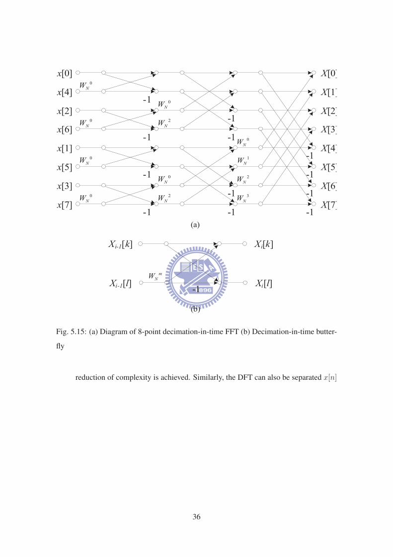
Fig. 5.15: (a) Diagram of 8-point decimation-in-time FFT (b) Decimation-in-time butter-
fly
reduction of complexity is achieved. Similarly, the DFT can also be separated x[n]
36
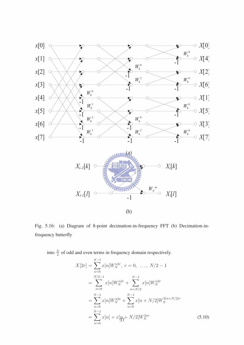
Fig. 5.16: (a) Diagram of 8-point decimation-in-frequency FFT (b) Decimation-in-
frequency butterfly
into N2
of odd and even terms in frequency domain respectively.
X[2r] =N−1∑
n=0
x[n]W n2rN , r = 0, . . . , N/2− 1
=
N/2−1∑
n=0
x[n]W n2rN +
N−1∑
n=N/2
x[n]W n2rN
=N−1∑
n=0
x[n]W n2rN +
N−1∑
n=0
x[n+N/2]W2(n+N/2)rN
=N−1∑
n=0
x[n] + x[n+N/2]W 2nrN (5.10)
37
X[2r + 1] =N−1∑
n=0
x[n]Wn(2r+1)N
=
N/2−1∑
n=0
x[n]Wn(2r+1)N +
N−1∑
n=N/2
x[n]Wn(2r+1)N
=N−1∑
n=0
x[n]Wn(2r+1)N +
N−1∑
n=0
x[n+N/2]W(n+N/2)(2r+1)N
=N−1∑
n=0
[x[n]− x[n+N/2]]Wn(2r+1)N (5.11)
The same as decimation-in-time algorithm, each N2
-point DFT is computed by
(5.10), (5.11) and N4
-point. Finally, we also obtain the diagram of 8-point decimation-
in-frequency FFT in Fig. 5.16(a) The basic decimation-in-frequency is shown in
Fig. 5.16(b) shows the diagram of 8-point decimation-in-frequency butterfly com-
putation.
• Radix-4 Algorithm
Radix-4 algorithm is base in radix-2 algorithm that usually uses in large N since
radix-2 algorithm in large N require too much computations. Radix-4 FFT algo-
rithm is more efficient computation than radix-2, but radix-4 needs N is power of
four and the butterfly computation is more complex than radix-2. Similarly to the
radix-2 algorithm decimates the N -point into four N4
as follows
X[k] =N−1∑
n=0
x[n]W nkN
=
N/4−1∑
n=0
x[n]W nkN +
N/2−1∑
n=N/4
x[n]W nkN +
3N/4−1∑
n=N/2
x[n]W nkN +
N−1∑
n=3N/4
x[n]W nkN
=
N/4−1∑
n=0
x[n]W nkN +
N/4−1∑
n=0
x[n+N/4]W(n+N/4)kN
+
N/4−1∑
n=0
x[n+N/2]W(n+N/2)kN +
N/4−1∑
n=0
x[n+ 3N/4]W(n+3N/4)kN
=
N/4−1∑
n=0
[x[n] + (−j)kx[n+N/4](−1)kx[n+N/2] + (j)kx[n+ 3N/4]]W nkN
(5.12)
38

The equation (5.12) is not related on N4
-point DFT because the twiddle factor de-
pends on N. Thus, we obtain the decimation-in-frequency (DIF) from (5.12). it
follows
X[4k] =
N/4−1∑
n=0
x[n] + x[n+N/4] + x[n+N/2] + x[n+ 3N/4]W nkN/4 (5.13)
X[4k + 1] =
N/4−1∑
n=0
x[n]− jx[n+N/4]− x[n+N/2] + jx[n+ 3N/4]W nkN W nk
N/4
(5.14)
X[4k + 2] =
N/4−1∑
n=0
x[n]− x[n+N/4] + x[n+N/2]− x[n+ 3N/4]W 2nkN W nk
N/4
(5.15)
X[4k] =
N/4−1∑
n=0
x[n] + jx[n+N/4]− x[n+N/2]− jx[n+ 3N/4]W 3nkN W nk
N/4
(5.16)
Then it has four N4
-point DFTs that we can obtain the basic radix-4 butterfly ac-
cording to (5.13), (5.14), (5.15), (5.16) as shown in Fig. 5.17(a)
Fig. 5.17(b) shows the diagram of 16-point radix-4 FFT algorithm.
5.6 FFT Architecture for Implementation
In section 5.5, we have introduced several FFT algorithm. It is important to choose the
proper architecture for requirement of function. In this section we will introduce the
architecture of FFT. They can be classified roughly into two types: the pipeline and the
memory-based architecture.
5.6.1 Memory-based Architecture
The Purpose of the memory-based architecture is increasing the reusable rate of memory
and butterfly processing element(PE). Fig. 5.18 is the block diagram of memory-based
architecture. It is composed by controller, processing element, address generator, RAM,
and ROM. The controller control the RAM and ROM to read or write, and control the
39

Fig. 5.17: (a) Radix-4 decimation-in-frequency butterfly (b) Diagram of 16-point radix-4
DIF FFT
40

address generator to generate the specific address to RAM and ROM by difference stage
of FFT. RAM store the data of FFT. ROM store the twiddle factor.
At first, RAM receives the input data, then according to the address which address
generator produces, RAM and ROM read data to the PE to perform the butterfly compu-
tation. The result after PE in-place to the same RAM address. In general, it requires one
PE to provide whole FFT.
Fig. 5.18: Block diagram of memory-based architecture
5.6.2 Pipeline Architecture
The pipeline architecture has two types: single-path delay feedback (SDF) and multi-
path delay commutator (MDC) [21]. Both of them use a series of register as the delay
buffer. Fig. 5.19 shows the pipeline architecture of SDF for radix-2 algorithm. Unlike
the memory-based FFT architecture, SDF pipeline architecture can apply various FFT
algorithm and maintain the regularity. SDF also has higher throughput than memory-
41

Fig. 5.19: Radix-2 DIF SDF
Fig. 5.20: SDF operation modes (a) mode1 (b) mode2
based but requires more hardware cost. The SDF operation has two modes shown in
Fig. 5.20. Fig. 5.21 shows the block diagram of multi-path delay commutator (MDC).
Fig. 5.21: Radix-2 DIF MDC
MDC separate the input data into two parallel data streams, one directly output to the
next stage, another multiply the coefficient. Using the switch to achieve the butterfly
computation. In general, MDC architecture has higher throughput than SDF.
5.7 Heart Rate Estimator
The primary module of heart rate estimator is FFT and IFFT modules. We can apply IFFT
by FFT since FFT and IFFT architecture are similarly. Thus we introduce the proposed
42

FFT module in this section.
• FFT requirements:
Before we construct the FFT module, we have to define the specification from re-
quirement of heart rate estimation system. In order to evaluate the heart rate, it
must have two R waves to represent the R-R interval. The worst case is the R wave
occurring in middle. The situation is shown in Fig. 5.22. The sampling frequency
Fig. 5.22: The worst case of situation
is 512Hz and the minimum heart rate that we can estimate, set to be 30 per minute.
Therefore, we need 4096-point FFT processor since it also has 2048-point zero
padding. Thus, the FFT block diagram is shown in Fig. 5.23
We adopt the memory-based FFT architecture since the system operates in low
frequency and needs low power and area for wearable system. The basic butterfly
computation uses radix-4 algorithm and it is more efficient than radix-2.
In the FFT module, we use four states as shown in Fig. 5.24 First state is idle, it is a reset
state that reset the FFT module to initial value. When IN VALID is high, FFT processor
starts to receive the input data and the state change to input state . Then, when input
completely, the input s is high and enters to the compute state to compute the FFT. It
outputs the result at output state and returns to idle.
43

Fig. 5.23: Proposed FFT block diagram
Fig. 5.24: State flow chart of the FFT module
44
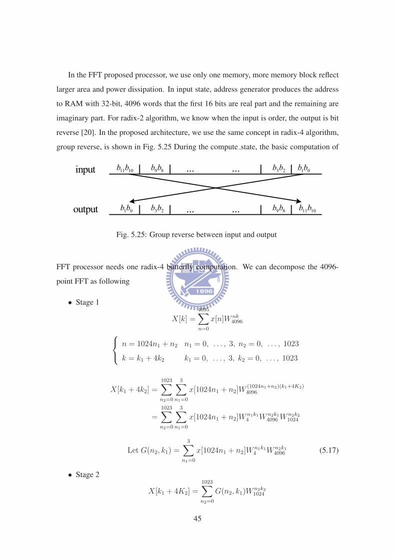
In the FFT proposed processor, we use only one memory, more memory block reflect
larger area and power dissipation. In input state, address generator produces the address
to RAM with 32-bit, 4096 words that the first 16 bits are real part and the remaining are
imaginary part. For radix-2 algorithm, we know when the input is order, the output is bit
reverse [20]. In the proposed architecture, we use the same concept in radix-4 algorithm,
group reverse, is shown in Fig. 5.25 During the compute state, the basic computation of
Fig. 5.25: Group reverse between input and output
FFT processor needs one radix-4 butterfly computation. We can decompose the 4096-
point FFT as following
• Stage 1
X[k] =4095∑
n=0
x[n]W nk4096
n = 1024n1 + n2 n1 = 0, . . . , 3, n2 = 0, . . . , 1023
k = k1 + 4k2 k1 = 0, . . . , 3, k2 = 0, . . . , 1023
X[k1 + 4k2] =1023∑
n2=0
3∑
n1=0
x[1024n1 + n2]W(1024n1+n2)(k1+4K2)4096
=1023∑
n2=0
3∑
n1=0
x[1024n1 + n2]Wn1k14 W n2k1
4096 Wn2k21024
Let G(n2, k1) =3
∑
n1=0
x[1024n1 + n2]Wn1k14 W n2k1
4096 (5.17)
• Stage 2
X[k1 + 4K2] =1023∑
n2=0
G(n2, k1)Wn2k21024
45

n2 = 256n3 + n4 n3 = 0, . . . , 3, n4 = 0, . . . , 255
k2 = k3 + 4k4 k3 = 0, . . . , 3, k4 = 0, . . . , 255
X[k1 + 4k3 + 16k4] =255∑
n4=0
3∑
n3=0
G(256n3 + n4, k1)W(256n3+n4)(k3+4k4)1024
=255∑
n4=0
3∑
n3=0
G(256n3 + n4, k1)Wn3k34 W n4k3
1024 Wn4k4256
Let H(n4, k1, k3) =3
∑
n3=0
G(256n3 + n4, k1)Wn3k34 W n4k3
1024 (5.18)
• Stage 3
X[k1 + 4k3 + 16k4] =255∑
n4=0
H(n4, k1, k3)Wn4k4256
n4 = 64n5 + n6 n5 = 0, . . . , 3, n6 = 0, . . . , 63
k4 = k5 + 4k6 k5 = 0, . . . , 3, k6 = 0, . . . , 63
X[k1 + 4k3 + 16k5
+64k6] =63∑
n6=0
3∑
n5=0
H(64n5 + n6, k1, k3)W(64n5+n6)(k5+4k6)64
=63∑
n6=0
3∑
n5=0
H(64n5 + n6, k1, k3)Wn5k54 W n6k5
256 W n6k664
Let I(n6, k1, k3, k5) =3
∑
n5=0
H(64n5 + n6, k1, k3)Wn5k54 W n6k5
256 (5.19)
• Stage 4
X[k1 + 4k3 + 16k5 + 64k6] =63∑
n6=0
I(n6, k1, k3, k5)Wn6k664
n6 = 16n7 + n8 n7 = 0, . . . , 3, n8 = 0, . . . , 15
k6 = k7 + 4k8 k7 = 0, . . . , 3, k8 = 0, . . . , 15
46

X[k1 + 4k3 + 16k5
+64k7 + 256k8] =15∑
n8=0
3∑
n7=0
I(64n7 + n8, k1, k3, k5)W(16n7+n8)(k7+4k8)64
=15∑
n6=0
3∑
n5=0
I(64n7 + n8, k1, k3, k5)Wn7k74 W n8k7
64 W n8k816
Let J(n8, k1, k3, k5, k7) =3
∑
n7=0
I(64n7 + n8, k1, k3, k5)Wn7k74 W n8k7
64 (5.20)
• Stage 5
X[k1 + 4k3 + 16k5 + 64k7 + 256k8] =15∑
n8=0
J(n8, k1, k3, k5, k7)Wn8k816
n8 = 4n9 + n10 n9 = 0, . . . , 3, n10 = 0, . . . , 3
k8 = k9 + 4k10 k9 = 0, . . . , 3, k10 = 0, . . . , 3
X[k1 + 4k3 + 16k5
+64k7 + 256k9
+1024k10] =3
∑
n10=0
3∑
n9=0
J(4n9 + n10, k1, k3, k5, k7)W(4n9+n10)(k9+4k10)16
=3
∑
n10=0
3∑
n9=0
J(4n9 + n10, k1, k3, k5, k7)Wn9k94 W n10k9
16 W n10k104
Let K(n10, k1, k3, k5, k7, k9) =3
∑
n9=0
J(4n9 + n10, k1, k3, k5, k7)Wn9k94 W n10k9
16
(5.21)
• Stage 6
X[k1 + 4k3 + 16k5 + 64k7
+256k9 + 1024k10] =3
∑
n10=0
K(n10, k1, k3, k5, k7, k9)Wn10k104 (5.22)
The property of twiddle factor is symmetry, we only need 1/8 twiddle factors in ROM.
Fig. 5.26 shows the symmetry property of twiddle factor zone 0 are kept in ROM, other
seven zones are converted from the twiddle factor in zone 0.
47

Fig. 5.26: The symmetry property of twiddle factor
In butterfly computation we use 26 adders and 4 multiplier. Each computation for
butterfly needs 4 clocks to read and 4 clocks to write back. For memory assignment, we
propose a way to generate the address for RAM and ROM without computation. During
FFT computation, the counter accumulates for each stage, we use the counter to produce
the address that group slide the counter. Fig. 5.27 depicts the addressing algorithm of
FFT. Where C11, C10, . . . , C1 are bits of counter. From equation (5.17)–(5.22), we know
in the stage 1, the address of RAM is the same as counter. Stage 2 c11c10 move to LSB and
other bits shift left 2 bits. perform the same thing for each stage can produce the address
for RAM.
For the same reason, ROM address can also produce by counter without computation.
From (5.17)–(5.22), we know W n2k14096 ,W n4k3
1024 ,W n6k5256 W n8k7
64 ,W n10k916 are twiddle factors that
keeps in ROM. The ROM address assignment can provide by counter in Fig. 5.28.
The inverse FFT (IFFT) can be realized by the same architecture of FFT. the IDFT
formula is given by
x[n] =1
N
N−1∑
k=0
X[k]W−nkN (5.23)
48

Fig. 5.27: RAM address assignment of FFT
Fig. 5.28: ROM address assignment of FFT
49

Multiplying both sides of (5.23) by N, we have
Nx[n] =N−1∑
k=0
X[k]W−nkN
Nx∗[n] =N−1∑
k=0
X∗[k]W nkN
=N−1∑
k=0
X[k]W nkN if X[k] is real (5.24)
Thus, we can perform the IFFT by computing FFT directly.
5.8 Experimental and Result
Fig. 5.29: Brief system specifications
The brief system specifications are shown in Fig 5.29. After we design the FFT mod-
ule and apply to real time heart rate estimation system, we compile the RTL code to FPGA
and the compile report is shown in Fig. 5.30. In the report, we use 7541 logic elements
which is 23 percent of the total logic elements in this FPGA board. And the used regis-
ters occupies 8 percent of all dedicate logic registers. The usage of on-chip memory is
38 percent. The result display on the FPGA device is shown in Fig. 5.31 The first three
seven-segment display that express the signal quality indicator is 0.94. The best is 1, and
the other three seven-segment display show the heart rate, 74 heartbeats per minute.
50

Fig. 5.30: Compile report of the entire system
Fig. 5.31: Results display on the FPGA device
51

Chapter 6
Conclusion and Future Work
In this thesis, we focus on a memory-based architecture FFT design for the heart rate
estimator. We use one single-port memory block to achieve radix-4 FFT, and the memory
address assignment depends on a counter and current stage. We reduce the complexity of
the address generator and apply it in low frequency system.
In the future work, The system can add the function of wireless transmission that can
be transmitted to central terminal and can then be analyzed the waveform by computers or
cellphones. In FPGA implementation, real-value architecture may be applied in system
to increase the efficiency and reduce the power dissipation of the system. Consider the
long FFT idle time since we estimate the heart rate every 512 samples, the FFT can use
more clock cycle to compute FFT and IFFT and reduce the power consumption and area
of FFT module. For minimizing the area of the system, we can design an application
specific integrated circuit (ASIC) that incorporate with the front-end circuits and A/D
converter.
52

Bibliography
[1] M Di Rienzo, F Rizzo, G Parati, M Ferratini, G Brambilla, and P Castiglioni “A
Textile-Based Wearable System for Vital Sign Monitoring: Applicability in Cardiac
Patients ” Computers in Cardiology, pp. 699V701, 2005.
[2] H. Ding, S. Crozier, and S. Wilson, “A New Heart Rate Variability Analysis Method
by Means of Quantifying the Variation of Nonlinear Dynamic Patterns,” IEEE Trans-
actions on Biomedical Engineering, vol. 54, no. 9, 2007.
[3] K. Hung, Y. T. Zhang, and B. Tai, “Wearable Medical Devices for Tele-Home
Healthcare”, Proc. of 26th Int. Conf. IEEE EMBS, San Francisco, pp. 5384-5387,
Sept. 2004.
[4] J. Muhlsteff, O. Such, R. Schmidt, M. Perkuhn, H. Reiter, J. Lauter, J. Thijs, G.
Musch, M. Harris, “Wearable approach for continuous ECG - and activity patient-
monitoring”, 2004. IEMBS ’04. 26th Annual International Conference of the IEEE
Engineering in Medicine and Biology Society, 2004, pp. 2184-2187. 2004.
[5] L. Grajales, I.V. Nicolaescu, “Wearable multisensor heart rate monitor” International
Workshop on Wearable and Implantable Body Sensor Networks, pp. 153-157, 2006.
[6] Kher, R. Vala, D. Pawar, T. Thakar, V.K. “Implementation of derivative based QRS
complex detection methods” 2010 3rd International Conference on Biomedical En-
gineering and Informatics (BMEI), pp. 927-931, 2010.
[7] Dinh, H.A.N. Kumar, D.K. Pah, N.D. Burton, P. “ Wavelets for QRS detection”
Proceedings of the 23rd Annual International Conference of the IEEE Engineering
in Medicine and Biology Society, 2001, pp. 1883-1887, 2001.
53

[8] Ji-Le Hu, Shu-Di Bao, “An approach to QRS complex detection based on multi-
scale mathematical morphology” 2010 3rd International Conference on Biomedical
Engineering and Informatics (BMEI), pp. 725-729, 2010
[9] J. G. Webster, Medical Instrumentation Application and Design, John Wiley and
Sons, Inc., 1998.
[10] G. H. Golub and C. F. Van Loan, Matrix Computation, Baltimore, MD: John Hop-
kins University Press, 1989.
[11] M. H. Cheng, L. C. Chen and Y. C. Hung, “A Real-Time Heart-Rate Estimator
from Steel Textile ECG Sensors in a Wireless Vital Wearing System,” 2nd Int. Conf.
Bioinformatics and Biomedical Engineering, Shanghai, China, May 2008.
[12] B-U Kohler et al, “The principles of software QRS detection,” IEEE Eng. in
Medicine and Biology Magazine, vol. 21, pp. 42-57, Jan. 2002.
[13] C. Li, C. Zheng, and C. Tai, Detection of ECG characteristic points using Wavelet
Transforms, IEEE Transactions on Biomedical Engineering, vol. 42, no. 1, pp. 21-
28, Jan., 1995.
[14] V. X. Afonso, W. J. Tompkins, T. Q. Nguyen, and S. Luo. “ECG Beat Detection
using Filter Banks”. IEEE Trans. on Biomedical Engineering, 46(2):192-202, Feb.
1999.
[15] P. Maragos and R. W. Schafer. “Morphological Systems for Multidimensional Signal
Processing.” Proceedings of the IEEE, 78(4):690-710, April 1990.
[16] Leland B. Jackson Digital Filters and Signal Processing, Kluwer Academic Publish-
ers, 1996.
[17] M. E. Van Valkenburg, Analog Filter Design, Oxford University Press, 1995.
[18] N. Weste and D. Harris, CMOS VLSI Design: A Circuits and Systems Perspective,
Addison Wesley, 2004.
54

[19] J. W. Cooley and J. W. Tukey, “An Algorithm for the Machine Calculation of Com-
plex Fourier Series,” Math.Comp., Vol. 19, pp. 297-301, April 1965.
[20] Alan V. Oppenheim and Ronald W. Schafer, Discrete-Time Signal Processing, Pren-
tice Hall International, Inc., 1999.
[21] S. He and M. Torkelson, “Design and implementation of a 1024-point pipeline FFT
processor,” in Proc. IEEE Custom Integrated Circuits Conf., pp. 131-134, May 1998
55


![(d) Decompose surface into multi-resolution surfaces [1]](https://img.pdfslide.us/doc/110x75/56813428550346895d9b167e/d-decompose-surface-into-multi-resolution-surfaces-1.jpg)