00T Wes Gray Jack Vogel Cross Section Predictability

7/17/2019 00T Wes Gray Jack Vogel Cross Section Predictability

http://slidepdf.com/reader/full/00t-wes-gray-jack-vogel-cross-section-predictability 1/26

The Cross-Section Predictability of Cyclically-Adjusted Valuation Measures1

Wesley R. GrayDrexel University101 N. 33rd Street

Academic Building 209Philadelphia, PA 19104

[email protected]

Jack Vogel

Drexel University101 N. 33rd

StreetAcademic Building 209Philadelphia, PA 19104

[email protected]

This Draft: February 28, 2014

First Draft: September 1, 2013

1 We would like to thank Steve LeCompte, Gary Antonacci, Mebane Faber, Marvin Kline, and David Foulke forhelpful comments and insights.

mailto:[email protected]







The Cross-Section Predictability of Cyclically-Adjusted Valuation Measures

ABSTRACT

Cyclically-adjusted valuation metrics predict cross-sectional variation in

average stock returns. For example, the annually-rebalanced top decile portfolio

ranked on Shiller P/E, or cyclically-adjusted price-to-earnings (CAPE) ratio, earns

an annual four-factor alpha of 2 percent a year. More frequent rebalancing and

momentum can generate alphas estimates of 8.1% a year. The inflation-adjustment

component of cyclically-adjusted measures has little effect on cross-sectional

predictability.

JEL Classification: G10, G12, G14

Key words: CAPE, long-term valuation metrics, value investing, market efficiency,Shiller P/E



1

Graham and Dodd (1934) suggest that the measure for earnings in a price to

earnings ratio “should cover a period of not less than five years, and preferably

seven to ten years.” Robert Shiller has taken the long-term P/E ratio concept from

Graham and Dodd one step further and suggests inflation-adjusting the past 10

years of earnings and comparing this long-term cyclically-adjusted earnings metric

to the current inflation-adjusted price. 1 The popularity of the Shiller’s P/E ratio, or

cyclically-adjusted P/E (CAPE),2 stems from its intuitive appeal and the empirical

evidence on the ratio’s ability to predict future market returns. For example,

Campbell and Shiller (1998c) show a strong negative correlation between CAPE

and future long-term stock market returns, on average.

Despite the intuitive appeal of the CAPE concept, there is no research we

know of that uses cyclically-adjusted valuation ratios to predict cross-sectional

variation in returns. Researchers have performed a battery of tests on other

valuation measures to identify their cross-sectional predictability. Examples

include Loughran and Wellman (2012), Gray and Vogel (2012), and Anderson and

Brooks (2006) in international markets.

Some evidence suggests that longer-term (i.e., less than 8 years) metrics are

not reliably better at predicting returns than one year metrics (Gray and Vogel

2012). However, previous authors have not tested the performance of ratios

1 See the calculations presented at http://www.econ.yale.edu/~shiller/data/ie_data.xls. Accessed September 11, 2013.2 E.g., “Have you looked at the Shiller P/E Ratio Lately,” Steven Russolillo, The Wall Street Journal, Accessed July23, 2013.



2

calculated using an inflation-adjustment, nor have previous researchers explored

the effectiveness of using a 10-year look-back period. The goal of this paper is to

fill this void in the academic literature.

We examine the following pricing metrics (all expressed in “yield” format

and all variables are inflation-adjusted by the Consumer Price Index (CPI):

• 10-year average real earnings to market capitalization (CA-EM)

• 10-year average real book values to market capitalization (CA-BM)

•

10-year average real earnings before interest and taxes and depreciation

and amortization to total enterprise value (CA-EBITDA/TEV)

• 10-year average real free cash flow to total enterprise value (CA-

FCF/TEV)

• 10-year average real free gross profits to total enterprise value (CA-

GP/TEV)

From July 1, 1973 through December 31, 2013, we find evidence that

cyclically-adjusted valuation metrics can predict cross-sectional stock returns. For

example, an annually-rebalanced equal weight portfolio of high CA-EM stocks

(top decile) earns 16.3% a year, while a portfolio of low CA-EM stocks (bottom

decile) earns 9.9% a year.3 This outperformance of the cheap cyclically-adjusted

3 Value weight portfolios yield similar results.



3

portfolios is consistent across the other measures, and is confirmed when

comparing Sharpe and Sortino ratios across the high and low portfolios.

We look at the performance of more frequently rebalanced stock portfolios

sorted on cyclically-adjusted valuations. Asness and Frazzini (2013) find that by

simply updating the price each month when computing the book-to-market ratio

yields 305 annual basis points of 4-factor alpha. Similar to Asness and Frazzini,

we updated the price (market capitalization) in our measures each month.

Employing a monthly rebalance enhances the performance of all valuation

measures. For example, the CA-EM strategy goes from a 16.3 percent compound

annual growth rate (CAGR) to a 19.3 percent CAGR.

We investigate the performance associated with combining momentum4 with

cyclically-adjusted valuation measures. Using the monthly-rebalanced portfolios,

we split each valuation decile into high and low momentum. Employing this

momentum sort enhances portfolio returns by approximately 100bps a year.

Last, we examine how the cyclical adjustment component affects returns

compared to a non-inflation-adjusted long-term valuation measure. The evidence

suggests that the cyclical adjusted component of 10-year valuation measures have

little effect on cross-sectional predictability. In fact, unadjusted 10-year valuation

measures are arguably stronger at predicting returns.

4 Jagadeesh and Titman (1993) have shown that momentum can predict variation in the cross section of stockreturns.



4

Our collective evidence confirms the effectiveness of using cyclically-

adjusted valuation metrics to identify high and low performing stocks.

Additionally, we find that more frequent rebalancing and momentum can enhance

performance. Last, we document that the inflation component of cyclically-

adjusted valuation ratios has little effect on cross-sectional predictability.

1. Data

1.1. Data Description

Our data sample includes all firms on the New York Stock Exchange

(NYSE), American Stock Exchange (AMEX), and Nasdaq firms with the required

data on CRSP and Compustat. We only examine firms with ordinary common

equity on CRSP and eliminate all REITS, ADRS, closed-end funds, and financial

firms. We incorporate CRSP delisting return data using the technique of Beaver,

McNichols, and Price (2007). To be included in the sample, all firms must have a

non-zero market value of equity as of June 30th

of year t . All valuation metrics

include 10 years of inflation-adjusted values for the numerator and the inflation-

adjusted price value for the denominator. In the case of CA-EBITDA/TEV, this is

represented by the following equation:

/10 =

∑ 10=1

10 10

(1)

The details on the construction of our valuation measures are as follows:



5

• Total Enterprise Value (TEV)

o Similar to the Loughran and Wellman (2011), we compute TEV

as:

TEV = Market Capitalization (M) + Short-term Debt

(DLC) + Long-term Debt (DLTT) + Preferred Stock

Value (PSTKRV) – Cash and Short-term Investments

(CHE). This variable is used in multiple valuation

measures.

• Earnings to Market Capitalization (E/M)

o Following Fama and French (2001), we compute earnings as:

Earnings = Earnings Before Extraordinary Items (IB) –

Preferred Dividends (DVP) + Income Statement Deferred

Taxes (TXDI), if available.

• Earnings before interest and taxes and depreciation and amortization

to total enterprise value (EBITDA/TEV)

o EBITDA = Operating Income Before Depreciation (OIBDP) +

Non-operating Income (NOPI).

• Free cash flow to total enterprise value (FCF/TEV)

o Similar to the Novy-Marx (2013) paper, we compute FCF and

as:



6

FCF = Net Income (NI) + Depreciation and Amortization

(DP) - Working Capital Change (WCAP (t) - WCAP (t-

1)) - Capital Expenditures (CAPX).

• Gross profits to total enterprise value (GP/TEV)

o Following Novy-Marx (2013), we compute GP as:

GP = Total Revenue (REVT) – Cost of Goods Sold

(COGS).

•

Book to market (B/M)

o Similar to Fama French (2001), we compute Book Equity as:

o Book Equity = Stockholder's Equity (SEQ) (or Common

Equity (CEQ) + Preferred Stock Par Value (PSTK) or

Assets (AT) - Liabilities (LT)) – Preferred Stock (defined

below) + Balance Sheet Deferred Taxes and Investment

Tax Credit (TXDITC) if available.

Preferred Stock = Preferred Stock Redemption

Value (PSTKRV) (or Preferred Stock Liquidating

Value (PSTKL), or Preferred Stock Par Value

(PSTK)).

The sample only includes those firms that have 10 years of data for all the

necessary metrics described above. To ensure there is a baseline amount of



7

liquidity in the securities in which we perform our tests, we restrict our analysis to

firms that are greater than the 40th

percentile NYSE market equity breakpoint on

June 30th of each year, which leaves 750 firms in the universe on average.

Stock returns are measured from July 1973 through December 2013. Firm

size (market capitalization) is determined on June 30th of year t. Firm

fundamentals are based on December 31st of year t-1 (for firms with fiscal year

ends between January 1st and March 31st we use year t fundamentals; for firms with

fiscal year ends after March 31st

we use year t-1 fundamentals). Firms are sorted

into deciles on each measure on June 30th of year t, and this value is used to

compute the monthly returns from July 1st of year t to June 30th of year t+1. Equal-

weight portfolio returns are buy and hold.

For the monthly-rebalanced portfolios, firm market capitalization is

calculated each month, while keeping the same firm fundamentals. For example,

the book value of equity would remain the same from July 1 st of year t to June 30th

of year t+1, while the market capitalization would be recalculated each month.

Total enterprise value, or TEV, would be computed similarly, with the market

capitalization changing each month, while the other variables would remain the

same from July 1st of year t to June 30th of year t+1. This portfolio is rebalanced

each month.



8

Figure 1 highlights the value-weight cyclically-adjusted valuation metrics

over time for stocks in our universe. The measures have been scaled to 100 as of

July 1, 1973 to facilitate a visual comparison. All ratios are highly correlated and

exhibit similar trends over time. One notable exception is CA-FCF/TEV, which

signals a much more expensive market during the ‘80s relative to the other

valuation measures. We also plot the rolling 12-month growth in the consumer

price index (CPI). The rolling inflation figure appears correlated with market

valuation measures.

[Insert Figure 1]

2. Results: A Comparison of Cyclically-Adjusted Valuation Metrics

2.1. Annual Rebalance

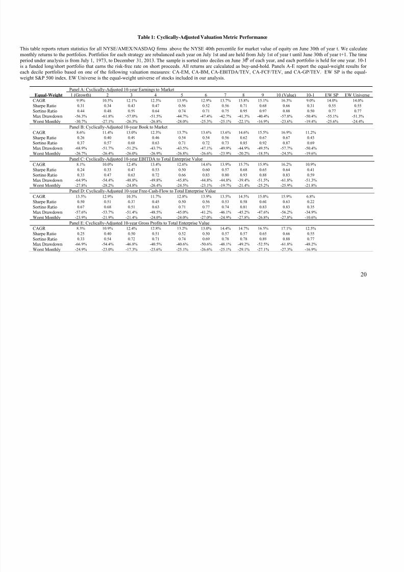
We present common performance metrics in Table 1. All valuation metrics

predict cross-sectional returns across the 10 decile portfolios. Each decile contains

75 firms, on average. There is a monotonic relationship between cyclically-

adjusted long-term valuation ratios and portfolio performance. The one exception

to this rule is CA-FCF/TEV, which has weak performance compared to the other

measures. The cyclically-adjusted free-cash-flow based valuation measure is

unable to identify the winners and losers within the cross-section.5

5 The FCF results are consistent with Novy-Marx (2013), which examines one-year FCF valuation metrics and finds



9

[Insert Table 1]

With respect to the most expensive stocks (i.e., “growth”), the results

suggest that buying expensive securities is a poor risk-adjusted bet. Compound

annual growth rates (CAGR), maximum drawdowns, Sharpe and Sortino ratios are

uniformly worse for expensive stocks relative to cheap stocks, regardless of the

cyclically-adjusted valuation metric employed. Moreover, on every metric, the

expensive stocks underperform the buy-and-hold benchmarks.

Buying the cheapest stocks on a cyclically-adjusted ratio basis performs

well, regardless of the chosen methodology. Figure 2 shows the growth of $100

invested into each of the top decile (cheap) portfolios as of 7/1/1973. Similar to

Table 1, this figure highlights the relative outperformance of the cyclically-

adjusted measures compared to an equal-weight benchmark portfolio. The cross-

sectional predictability is marginally stronger for stocks sorted on cyclically-

adjusted B/M and GP/TEV, which exhibit the largest CAGR spreads between the

top and bottom deciles. 6

[Insert Figure 2]

2.2. Monthly Rebalance

Table 2 reports performance statistics for monthly-rebalanced portfolios

using cyclically-adjusted valuation metrics. The monthly results do not account for

low cross-sectional predictability.6 In non-tabulated results we look at robustness across time periods. Results are quantitatively similar.



10

taxes or transaction costs, which are assumed to be higher relative to the annually-

rebalanced results discussed in section 2.1. Similar to Table 1, we see a monotonic

relationship between cheapness and portfolio performance. Compound annual

growth rates (CAGR), maximum drawdowns, Sharpe and Sortino ratios are

uniformly worse for expensive stocks relative to cheap stocks. The monthly-

rebalance (MR) strategy has a higher CAGR, Sharpe ratio, and Sortino ratio for the

monthly-rebalanced strategy (Table 2), compared to the annual-rebalanced strategy

(Table 1). This finding corroborates the result found in Asness and Frazzini

(2013), which highlights that rebalancing portfolios each month improves portfolio

performance.

The performance for the monthly-rebalanced portfolios is again marginally

better for the cheapest cyclically-adjusted B/M and GP/TEV portfolios, which

corroborates the results in Table 1. Examining the CA-B/M measure, the monthly

CAGR, Sharpe and Sortino ratio are 19.7 percent (16.9 percent), 0.72 (0.67), and

1.09 (0.87) for the monthly (annual) rebalanced portfolio.7 The improvement from

annual to monthly rebalance is consistent across the other four measures as well.

2.3. Monthly Rebalance – Splitting on Momentum

Next, we split each cyclically-adjusted valuation decile by momentum. We

rebalance the portfolios monthly. The results in Table 3 focus on the most

7 In non-tabulated results we look at robustness across time periods. Results are quantitatively similar.



11

expensive and cheapest decile of monthly-rebalanced cyclically-adjusted valuation

measures. We split the bottom and top decile on each cyclically-adjusted valuation

measure into high and low momentum using the cumulative returns from month -

12 to month -2, similar to Fama and French (2008). This creates portfolios with an

average of 37 firms.

Table 3 Panels A and B show common performance metrics for growth

(expensive) stock portfolios split into low and high momentum. Similar to prior

research on momentum, we find that high momentum firms beat low momentum

firms. The low momentum portfolio has a lower CAGR, Sharpe ratio and Sortino

ratio compared to the high momentum portfolio for four of the five measures (the

exception is CA-FCF/TEV). Panel A (B) shows that the low (high) momentum

growth CA-EM (inverse of CAPE) firms earns a 7.0 percent (11.9 percent) CAGR,

has a 0.19 (0.37) Sharpe ratio, and a 0.28 (0.55) Sortino ratio.

Table 3 Panels C and D show common performance metrics for value

(cheap) stock portfolios split into low and high momentum respectively. Across all

five measures, the low momentum portfolio has a lower CAGR, Sharpe ratio and

Sortino ratio compared to the high momentum portfolio. Panel C (D) shows that

the low (high) momentum value CA-EM (inverse of CAPE) firms earns a 17.6

percent (20.7 percent) CAGR, has a 0.58 (0.82) Sharpe ratio, and a 0.92 (1.17)

Sortino ratio.



12

The data suggests that splitting portfolios on momentum can systematically

improve returns to the cyclically-adjusted valuation measures. When comparing

the monthly-rebalanced value portfolios (Table 2, Column 10 (Value)) to the high

momentum monthly-rebalanced value portfolios (Table 3, Panel D), we find that

value momentum portfolios have higher performance statistics, as the returns

improve from 19.3% to 20.7%.

2.4. Alpha Analysis

We implement a calendar-time portfolio regression approach advocated by

Mitchell and Stafford (2000). We calculate the monthly returns to the portfolios in

excess of the risk-free rate and regress this variable on a linear asset pricing model,

which include the following variables: MKT (excess value-weighted market index

return), SMB (small minus big), HML (high book-to-market minus low book-to-

market), and MOM (high momentum minus low momentum).8

[Insert Table 4]

The estimated alphas from our calendar-time portfolio regressions are

presented in Table 4. Panels A and B examine the alpha for the annually-

rebalanced bottom and top deciles respectively. Panel A reports an insignificant

negative alpha for the bottom decile, while Panel B reports a significant alpha for

the top decile (0.168% per month for the CA-EM measure). Panels C and D

8 See Fama and French (1993) and Carhart (1997). Factors obtained from Ken French’s websitehttp://mba.tuck.dartmouth.edu/pages/faculty/ken.french/data_librar y.html,

http://mba.tuck.dartmouth.edu/pages/faculty/ken.french/data_library.html





13

examine the alpha for the monthly-rebalanced bottom and top deciles respectively.

Panel C again finds an insignificant negative alpha for the bottom decile, while

Panel D reports a positive and significant alpha for the top decile. For the CA-EM

measure, the alpha for the top decile increases from 0.168% (Panel B) to 0.540%

(Panel D) per month when switching from annual to monthly rebalancing. Last,

Panels E and F examine the alpha for the monthly-rebalanced portfolios which

include momentum. Panel E finds a larger, yet still insignificant, negative alpha for

the low momentum growth portfolio. Conversely, Panel F finds the largest positive

and significant alpha for the high momentum value portfolio. The CA-EM alpha

increases from 0.540% (Panel D) to 0.577% (Panel F) per month when adding the

momentum screen to the monthly rebalance. Overall, the alpha analysis confirms

that cyclically adjusted valuation help explain the cross-section of average stock

returns above and beyond the 4-factor Carhart asset pricing model.

2.5. Does the Inflation Adjustment Matter?

In this section we examine how cyclically-adjusted measures compare to a

non-cyclically adjusted valuation measure. All valuation metrics include 10 years

of values for the numerator and the price value for the denominator. In the case of

EBITDA/TEV, this is represented by the following equation:

/10 =

∑ 10=1

1010

(1)



14

Unlike the prior analysis, there is no inflation adjustment for the numerator and

denominator. Table 5 examines the equal-weight annually-rebalanced

portfolios for both the cyclically adjusted (Columns 2 and 4) and non-cyclically

adjusted (Columns 3 and 5) valuation measures. Panel A reports the CAGR, Panel

B reports the Sharpe ratio, and Panel C reports the 4-factor alphas for the

portfolios. Overall, one can see that the CAGR, Sharpe ratio, and monthly alpha

are similar for both the cyclically and non-cyclically adjusted valuation measures.

Specifically, examining the gross profits to total enterprise measure (GP/TEV), the

top decile returns 17.37% (17.08%), has a Sharpe ratio of 0.674 (0.661), and a

monthly alpha of 0.310% (0.284%) for the non-cyclically adjusted (cyclically

adjusted) measure. Overall, there does not appear to be a significant

outperformance of the cyclically adjusted measures compared to a non-cyclically

adjusted measure.

3. Conclusion

We confirm the effectiveness of using cyclically-adjusted valuation metrics to

predict the cross-sectional stock returns. We also document that more frequent

rebalancing and the addition of a momentum sort can enhance strategies based on

cyclically-adjusted valuation metrics. Last, we document that the inflation



15

adjustment component of long-term cyclically-adjusted measure has little effect on

cross-sectional predictability.



16

References

Anderson, Keith, and C. Brooks, “The Long-Term Price-Earnings Ratio.” Journal

of Business Finance & Accounting 37 (2006), 1063-1086.Asness, Cliff, and A. Frazzini, “The Devil in HML’s Details.” Journal of Portfolio

Management 39 (2013), 49-68.Beaver, William, M. McNichols, and R. Price, “Delisting Returns and Their Effect

on Accounting-Based Market Anomalies.” Journal of Accounting and

Economics 43 (2007), 341-368.Campbell, J.Y., and Shiller, R.J., “The dividend-price ratio and expectations of

future dividends and discount factors.” Review of Financial Studies 1(1998a), 195–228.

Campbell, J.Y., and Shiller, R.J., “Stock prices, earnings, and expected dividends.” Journal of

Finance 43 (1998b), 661–676.Campbell, J.Y., and Shiller, R.J., “Valuation Ratios and the Long-Run Stock

Market Outlook.” Jounral of Portfolio Management 24 (1998c), 11-26.Carhart, Mark, “On Persistence in Mutual Fund Performance.” The Journal of

Finance 52 (1997), 57-82.Fama, Eugene F., and K. French, “Disappearing Dividends: Changing Firm

Characteristics or Lower Propensity to Pay?” Journal of Financial

Economics 60 (2001), 3-43.Fama, Eugene F., and Kenneth R. French, “The Cross-Section of Expected Stock

Returns.”The Journal of Finance 47 (1992), 427–465.

Fama, Eugene F., and Kenneth R. French, “Dissecting Anomalies.” The Journal of

Finance 63 (2008), 1653–1678.

Graham B., D. Dodd. Security Analysis, New York: McGraw-Hill, 1934.Gray, Wesley, and J. Vogel, “Analyzing Valuation Measures: A Performance

Horse Race over the Past 40 Years.” Journal of Portfolio Management 39(2012), 112-121.

Jagadeesh, Narasimhan, and Sheridan Titman, “Returns to buying winners and

sellingLosers: Implications for stock market efficiency.” The Journal of Finance 48(1993), 65-91.

Loughran, Tim, and J. Wellman, “New Evidence on the Relation Between theEnterprise Multiple and Average Stock Returns.” Journal of Financial and

Quantitative Analysis 46 (2012), 1629-1650.



17

Malkiel, B.G., A Random Walk Down Wall Street (Revised edition). W.W. Norton, NewYork, 2011.

Mitchell, Mark L., and E. Stafford, 2000, Managerial Decisions and Long-TermStock

Price Performance, Journal of Business 73, 287-329. Novy-Marx, Robert, “The Other Side of Value: Good Growth and the Gross

Profitability Premium.” Journal of Financial Economics 108 (2013), 1-28.



18

Figure 1: Cyclically-adjusted valuation metrics over time

This figure plots the value-weighted monthly cyclically-adjusted valuation metric for all NYSE/AMEX/NASDAQ firms above the NYSE 40th percentile formarket value of equity on June 30th of year t (left-axis). Cyclically-adjusted values are an average of inflation-adjusted values over ten years relative to aninflation-adjusted current market price or total enterprise value. Rolling 1-Year CPI growth represents the rolling annual compound growth in the consumer priceindex (right-axis). All cyclically-adjusted metrics are scaled to 100 on 7/1/1973. Results are from 7/1/1973 to 12/31/2013.



19

Figure 2: Invested Growth (Log Scale)

This figure reports portfolio growth from July 1, 1973, to December 31, 2013. The sample is sorted into deciles on June 30 th of each year, and each portfolio isheld for one year. All returns are calculated as equal-weight buy-and-hold. The figure reports the growth of $100 for the top decile portfolio based on one of thefollowing cyclically-adjusted valuation measures: CA-EM, CA-BM, CA-EBITDA/TEV, CA-FCF/TEV, and CA-GP/TEV. We only include NYSE/AMEX/NASDAQ firms above the NYSE 40th percentile for market value of equity on June 30th of year t.



20

Table 1: Cyclically-Adjusted Valuation Metric Performance

This table reports return statistics for all NYSE/AMEX/NASDAQ firms above the NYSE 40th percentile for market value of equity on June 30th of year t. We calculatemonthly returns to the portfolios. Portfolios for each strategy are rebalanced each year on July 1st and are held from July 1st of year t until June 30th of year t+1. The time period under analysis is from July 1, 1973, to December 31, 2013. The sample is sorted into deciles on June 30th of each year, and each portfolio is held for one year. 10-1is a funded long/short portfolio that earns the risk-free rate on short proceeds. All returns are calculated as buy-and-hold. Panels A-E report the equal-weight results foreach decile portfolio based on one of the following valuation measures: CA-EM, CA-BM, CA-EBITDA/TEV, CA-FCF/TEV, and CA-GP/TEV. EW SP is the equal-weight S&P 500 index. EW Universe is the equal-weight universe of stocks included in our analysis.

Panel A: Cyclically-Adjusted 10-year Earnings to Market

Equal-Weight 1 (Growth) 2 3 4 5 6 7 8 9 10 (Value) 10-1 EW SP EW Universe

CAGR 9.9% 10.5% 12.1% 12.3% 13.9% 12.9% 13.7% 15.8% 15.1% 16.3% 9.0% 14.0% 14.0% Sharpe Ratio 0.31 0.34 0.43 0.47 0.56 0.52 0.56 0.71 0.68 0.66 0.31 0.55 0.55

Sortino Ratio 0.44 0.48 0.59 0.64 0.74 0.71 0.75 0.95 0.97 0.88 0.50 0.77 0.77

Max Drawdown -56.3% -61.8% -57.0% -51.5% -44.7% -47.4% -42.7% -41.3% -40.4% -57.8% -50.4% -55.1% -51.3%

Worst Monthly -30.7% -27.1% -26.3% -26.8% -28.0% -25.3% -25.1% -22.1% -16.9% -23.6% -19.4% -25.6% -24.4%

Panel B: Cyclically-Adjusted 10-year Book to Market

CAGR 8.6% 11.4% 13.0% 12.3% 13.7% 13.6% 13.6% 14.6% 15.5% 16.9% 11.2%

Sharpe Ratio 0.26 0.40 0.49 0.46 0.54 0.54 0.56 0.62 0.67 0.67 0.43

Sortino Ratio 0.37 0.57 0.68 0.63 0.71 0.72 0.73 0.85 0.92 0.87 0.69

Max Drawdown -68.9% -51.7% -51.2% -43.7% -43.5% -47.1% -49.9% -44.9% -49.5% -57.7% -50.4%

Worst Monthly -26.7% -26.4% -26.0% -26.9% -26.8% -26.6% -23.9% -20.2% -18.5% -24.5% -19.6%

Panel C: Cyclically-Adjusted 10-year EBITDA to Total Enterprise Value

CAGR 8.1% 10.0% 12.4% 13.4% 12.6% 14.6% 13.9% 15.7% 15.9% 16.2% 10.9%

Sharpe Ratio 0.24 0.33 0.47 0.53 0.50 0.60 0.57 0.68 0.65 0.64 0.41

Sortino Ratio 0.33 0.47 0.63 0.72 0.66 0.83 0.80 0.93 0.88 0.83 0.59

Max Drawdown -64.9% -54.4% -48.8% -49.8% -45.8% -44.8% -44.8% -39.4% -51.5% -61.8% -51.3%

Worst Monthly -27.8% -28.2% -24.8% -26.4% -24.5% -23.1% -19.7% -21.4% -25.2% -25.9% -21.8%

Panel D: Cyclically-Adjusted 10-year Free-Cash-Flow to Total Enterprise Value

CAGR 13.5% 12.9% 10.3% 11.7% 12.8% 13.9% 13.5% 14.5% 15.0% 15.9% 6.8%

Sharpe Ratio 0.50 0.51 0.37 0.45 0.50 0.56 0.53 0.58 0.60 0.63 0.22

Sortino Ratio 0.67 0.68 0.51 0.63 0.71 0.77 0.74 0.81 0.83 0.83 0.35

Max Drawdown -57.6% -53.7% -51.4% -48.5% -45.0% -41.2% -46.1% -45.2% -47.6% -56.2% -34.9%

Worst Monthly -23.9% -21.9% -21.4% -24.0% -24.0% -27.0% -24.9% -27.8% -26.8% -27.8% -10.6%

Panel E: Cyclically-Adjusted 10-year Gross Profits to Total Enterprise Value

CAGR 8.3% 10.9% 12.4% 12.8% 13.2% 13.0% 14.4% 14.7% 16.5% 17.1% 12.5%

Sharpe Ratio 0.25 0.40 0.50 0.51 0.52 0.50 0.57 0.57 0.65 0.66 0.55

Sortino Ratio 0.33 0.54 0.72 0.71 0.74 0.69 0.78 0.78 0.89 0.88 0.77

Max Drawdown -66.9% -54.4% -46.8% -40.5% -40.6% -50.6% -48.1% -49.2% -52.5% -61.8% -48.2%

Worst Monthly -24.9% -23.0% -17.3% -23.6% -25.1% -26.6% -25.1% -29.1% -27.1% -27.3% -16.9%



21

Table 2: Monthly Rebalanced Cyclically-Adjusted Valuation Metric Performance

This table reports return statistics for all NYSE/AMEX/NASDAQ firms above the NYSE 40th percentile for market value of equity on June 30th of year t. We calculatemonthly returns to the portfolios. Portfolios for each strategy are rebalanced at the end of each month. The time period under analysis is from July 1, 1973, to December31, 2013. The sample is sorted into deciles at the end of each month. 10-1 is a funded long/short portfolio that earns the risk-free rate on short proceeds. All returns arecalculated as buy-and-hold. Panels A-E report the equal-weight results for each decile portfolio based on one of the following valuation measures: CA-EM, CA-BM, CA-EBITDA/TEV, CA-FCF/TEV, and CA-GP/TEV. EW SP is the equal-weight S&P 500 index. EW Universe is the equal-weight universe of stocks included in ouranalysis.

Panel A: Cyclically-Adjusted 10-year Earnings to Market

Equal-Weight 1 (Growth) 2 3 4 5 6 7 8 9 10 (Value) 10-1 EW SP EW Universe

CAGR 9.5% 10.3% 11.4% 12.1% 12.9% 13.2% 15.1% 16.2% 17.6% 19.3% 12.3% 14.0% 14.0% Sharpe Ratio 0.29 0.33 0.40 0.46 0.51 0.52 0.63 0.70 0.76 0.71 0.49 0.55 0.55

Sortino Ratio 0.42 0.46 0.54 0.65 0.68 0.69 0.85 0.97 1.14 1.08 0.85 0.77 0.77

Max Drawdown -60.6% -61.5% -56.6% -48.7% -49.1% -44.4% -48.9% -48.3% -45.7% -65.0% -39.1% -55.1% -51.3%

Worst Monthly -31.1% -26.3% -28.1% -24.9% -26.9% -27.7% -23.9% -22.7% -18.5% -26.0% -17.2% -25.6% -24.4%

Panel B: Cyclically-Adjusted 10-year Book to Market

CAGR 7.8% 10.9% 12.6% 13.4% 13.3% 14.5% 13.8% 15.0% 16.7% 19.7% 15.1%

Sharpe Ratio 0.22 0.38 0.47 0.51 0.51 0.58 0.55 0.62 0.69 0.72 0.61

Sortino Ratio 0.32 0.54 0.66 0.69 0.69 0.77 0.73 0.84 1.01 1.09 1.00

Max Drawdown -70.4% -51.2% -48.3% -47.0% -50.8% -48.7% -55.4% -50.7% -55.4% -64.0% -43.3%

Worst Monthly -27.5% -26.4% -25.4% -26.7% -26.5% -25.7% -25.7% -23.3% -21.0% -24.4% -23.2%

Panel C: Cyclically-Adjusted 10-year EBITDA to Total Enterprise Value

CAGR 7.4% 9.5% 11.7% 12.8% 13.0% 14.6% 15.0% 16.8% 17.9% 19.1% 14.6%

Sharpe Ratio 0.21 0.31 0.43 0.50 0.51 0.59 0.62 0.70 0.72 0.70 0.60

Sortino Ratio 0.29 0.43 0.59 0.69 0.68 0.82 0.88 1.00 1.02 0.97 0.85

Max Drawdown -69.3% -50.9% -52.3% -47.4% -51.1% -49.3% -50.0% -45.5% -57.0% -66.4% -46.2%

Worst Monthly -29.0% -26.7% -26.1% -26.9% -25.3% -22.3% -17.9% -21.6% -21.6% -27.0% -26.5%

Panel D: Cyclically-Adjusted 10-year Free-Cash-Flow to Total Enterprise Value

CAGR 13.9% 12.9% 10.5% 11.5% 12.5% 13.4% 14.6% 14.3% 16.4% 18.2% 8.6%

Sharpe Ratio 0.49 0.50 0.38 0.43 0.48 0.52 0.57 0.56 0.64 0.68 0.41

Sortino Ratio 0.68 0.69 0.52 0.60 0.71 0.72 0.81 0.78 0.94 0.96 0.68

Max Drawdown -66.5% -56.6% -53.7% -44.7% -43.6% -47.3% -50.2% -52.4% -47.5% -58.6% -23.7%

Worst Monthly -25.8% -21.9% -21.9% -24.2% -23.7% -27.2% -25.4% -27.2% -26.7% -28.4% -7.7%

Panel E: Cyclically-Adjusted 10-year Gross Profits to Total Enterprise Value

CAGR 8.0% 10.4% 12.1% 11.8% 13.9% 13.7% 14.7% 16.3% 17.3% 19.7% 15.7%

Sharpe Ratio 0.24 0.37 0.48 0.45 0.54 0.53 0.57 0.63 0.66 0.72 0.73

Sortino Ratio 0.31 0.51 0.70 0.64 0.79 0.74 0.80 0.88 0.93 1.01 1.13

Max Drawdown -67.6% -54.0% -46.7% -49.6% -45.5% -57.1% -48.0% -50.6% -54.2% -66.6% -41.3%

Worst Monthly -25.9% -22.0% -18.0% -22.4% -22.4% -25.4% -26.9% -27.5% -28.1% -27.4% -17.0%



22

Table 3: Momentum and Monthly Rebalanced Cyclically-Adjusted Valuation Metrics

This table reports return statistics for all NYSE/AMEX/NASDAQ firms above the NYSE 40th percentile for marketvalue of equity on June 30th of year t. We calculate monthly returns to the portfolios. Portfolios for each strategy arerebalanced each month. The time period under analysis is from July 1, 1973, to December 31, 2013. Panels A-D reportthe equal-weight results based on one of the following valuation measures: CA-EM, CA-BM, CA-EBITDA/TEV, CA-FCF/TEV, and CA-GP/TEV. Growth (value) firms are the bottom (top) decile for each of the five measures. The top(bottom) decile portfolio is then split by momentum, which is calculated as the cumulative returns from month -12 tomonth -2. Panels A (C) shows the returns to the low momentum portfolio for growth (value) firms, while Panels B (D)shows the returns to the high momentum portfolio for growth (value) firms. SP 500 EW is the equal-weight S&P 500index. SP 500 is the S&P 500 index.

CA-EM CA-BM CA-EBIDTA/TEV CA-FCF/TEV CA-GP/TEV SP 500 EW SP 500

Panel A: Low Momentum Growth Firms

CAGR 7.0% 6.1% 5.1% 14.0% 6.6% 14.0% 14.0%

Sharpe Ratio 0.19 0.15 0.11 0.47 0.17 0.55 0.55

Sortino Ratio 0.28 0.21 0.15 0.67 0.23 0.77 0.77

Max Drawdown -68.6% -69.0% -71.6% -60.6% -71.0% -55.1% -51.3%

Worst Monthly -29.9% -25.9% -28.8% -24.5% -24.5% -25.6% -24.4%

Panel B: High Momentum Growth FirmsCAGR 11.9% 9.1% 9.9% 13.4% 9.1% 14.0% 14.0%

Sharpe Ratio 0.37 0.28 0.30 0.46 0.28 0.55 0.55

Sortino Ratio 0.55 0.39 0.43 0.65 0.37 0.77 0.77

Max Drawdown -57.9% -75.7% -67.8% -70.3% -65.0% -55.1% -51.3%

Worst Monthly -32.0% -29.1% -28.9% -28.4% -26.8% -25.6% -24.4%

Panel C: Low Momentum Value Firms

CAGR 17.6% 17.8% 17.8% 16.7% 18.2% 14.0% 14.0%

Sharpe Ratio 0.58 0.59 0.60 0.58 0.61 0.55 0.55

Sortino Ratio 0.92 0.92 0.88 0.84 0.86 0.77 0.77

Max Drawdown -71.3% -70.7% -67.8% -63.6% -73.4% -55.1% -51.3%

Worst Monthly -31.1% -30.0% -27.3% -27.5% -28.1% -25.6% -24.4%

Panel D: High Momentum Value Firms

CAGR 20.7% 21.1% 20.1% 19.5% 20.9% 14.0% 14.0%

Sharpe Ratio 0.82 0.81 0.78 0.76 0.80 0.55 0.55Sortino Ratio 1.17 1.21 1.03 1.05 1.14 0.77 0.77

Max Drawdown -58.0% -56.4% -64.0% -53.1% -58.5% -55.1% -51.3%

Worst Monthly -24.6% -27.2% -27.1% -29.2% -27.4% -25.6% -24.4%



23

Table 4: Calendar-Time Portfolio RegressionsThis table reports return statistics for all NYSE/AMEX/NASDAQ firms above the NYSE 40th percentile for market value of equity on June 30th of year t. Wecalculate monthly returns to the portfolios. Portfolios for each strategy are rebalanced either annually or monthly. The time period under analysis is from July 1,1973, to December 31, 2013 for panels A through E. Panels A through E report the equal-weight results for the bottom and top decile portfolios (growth andvalue) based on one of the following valuation measures: CA-EM, CA-BM, CA-EBITDA/TEV, CA-FCF/TEV, and CA-GP/TEV. The portfolios are formedusing either annually valuation measures (Panels A and B), monthly valuation measures, (Panels C and D), or monthly valuation measures combined withmomentum (Panels E and F). Portfolio formation and rebalancing is the same as in Table 1 (for Panels A and B), Table 2 (for Panels C and D), and Table 3 (forPanels E and F). Panels A through E report the 4-factor alpha. Average alphas are in monthly percent, p-values are shown below the coefficient estimates, and5% statistical significance is indicated in bold. Regression p-values use robust standard errors as computed in Davidson and MacKinnon (1993, pg. 553).

Panel A: Annual Rebalance - Growth Firms Panel B: Annual Rebalance - Value Firms

CA-EM CA-BM CA-EBIDTA/TEV CA-FCF/TEV CA-GP/TEV CA-EM CA-BM CA-EBIDTA/TEV CA-FCF/TEV CA-GP/TEV

Alpha -0.104 0.022 -0.039 -0.066 -0.115 0.168 0.164 0.193 0.192 0.2840.330 0.796 0.693 0.553 0.331 0.069 0.114 0.033 0.021 0.002

Market Return – RF 1.176 1.086 1.093 1.083 0.994 1.003 1.034 1.048 1.022 1.0520.000 0.000 0.000 0.000 0.000 0.000 0.000 0.000 0.000 0.000

SMB 0.428 0.157 0.291 0.301 0.255 0.253 0.295 0.274 0.379 0.3720.000 0.000 0.000 0.000 0.000 0.000 0.000 0.000 0.000 0.000

HML -0.215 -0.520 -0.547 0.486 -0.255 0.689 0.706 0.579 0.406 0.4720.000 0.000 0.000 0.000 0.000 0.000 0.000 0.000 0.000 0.000

MOM -0.013 -0.027 -0.016 -0.026 -0.012 -0.130 -0.099 -0.146 -0.115 -0.1630.707 0.271 0.571 0.484 0.734 0.000 0.002 0.000 0.000 0.000

Panel C: Monthly Rebalance - Growth Firms Panel D: Monthly Rebalance - Value Firms Alpha -0.026 -0.095 -0.098 0.112 -0.177 0.540 0.563 0.553 0.525 0.612

0.827 0.238 0.315 0.351 0.113 0.000 0.000 0.000 0.000 0.000Market Return – RF 1.195 1.082 1.084 1.128 1.007 1.058 1.092 1.103 1.076 1.102

0.000 0.000 0.000 0.000 0.000 0.000 0.000 0.000 0.000 0.000SMB 0.416 0.191 0.325 0.307 0.278 0.348 0.346 0.306 0.364 0.413

0.000 0.000 0.000 0.000 0.000 0.000 0.000 0.000 0.000 0.000HML -0.261 -0.498 -0.551 0.455 -0.209 0.696 0.675 0.521 0.377 0.430

0.000 0.000 0.000 0.000 0.000 0.000 0.000 0.000 0.000 0.000MOM -0.136 0.026 -0.002 -0.238 0.004 -0.404 -0.399 -0.366 -0.344 -0.364

0.011 0.281 0.934 0.000 0.899 0.000 0.000 0.000 0.000 0.000

Panel E: Monthly Rebalance - Low Momentum Growth Firms Panel F: Monthly Rebalance - High Momentum Value Firms

Alpha -0.162 -0.179 -0.184 0.267 -0.211 0.577 0.602 0.590 0.583 0.6770.285 0.082 0.099 0.064 0.118 0.000 0.000 0.000 0.000 0.000

Market Return – RF 1.209 1.041 1.058 1.108 0.963 1.007 1.058 1.053 1.054 1.0410.000 0.000 0.000 0.000 0.000 0.000 0.000 0.000 0.000 0.000

SMB 0.319 0.118 0.292 0.341 0.228 0.250 0.245 0.220 0.300 0.3510.000 0.008 0.000 0.000 0.000 0.000 0.000 0.000 0.000 0.000

HML -0.096 -0.379 -0.513 0.459 -0.023 0.652 0.636 0.487 0.356 0.3720.307 0.000 0.000 0.000 0.727 0.000 0.000 0.000 0.000 0.000

MOM -0.281 -0.074 -0.153 -0.430 -0.176 -0.245 -0.244 -0.246 -0.251 -0.2580.000 0.021 0.000 0.000 0.000 0.000 0.001 0.000 0.000 0.000



24

Table 5: Cyclically versus non-cyclically adjusted measures

This table reports return statistics for all NYSE/AMEX/NASDAQ firms above the NYSE 40th percentile for marketvalue of equity on June 30th of year t. We calculate monthly returns to the portfolios. Portfolios for each strategy arerebalanced annually. The time period under analysis is from July 1, 1973, to December 31, 2013 for panels A throughC. Panels A through C report the equal-weight results for the bottom and top decile portfolios (growth and value) based on one of the following valuation measures: CA-EM, CA-BM, CA-EBITDA/TEV, CA-FCF/TEV, and CA-GP/TEV. The valuation measures are computed using either cyclically adjusted (columns 2 and 4) or non-cyclicallyadjusted (columns 3 and 5) valuation measures. Panel A reports the compound annual growth rate (CAGR), Panel Breports the Sharpe ratio, and Panel C reports the 4-factor alpha. Average alphas are in monthly percent, p-values areshown below the coefficient estimates, and 5% statistical significance is indicated in bold. Regression p-values userobust standard errors as computed in Davidson and MacKinnon (1993, pg. 553).

Growth Value

Panel A CAGR CAGR

CyclicallyAdjusted

Non-CyclicallyAdjusted

CyclicallyAdjusted

Non-CyclicallyAdjusted

P/E 9.86% 9.35% 16.35% 16.52%

B/M 8.62% 8.43% 16.91% 16.38%

EBITDA/TEV 8.08% 8.10% 16.25% 16.22%

FCF/TEV 13.48% 12.62% 15.85% 16.01%

GP/TEV 8.28% 8.24% 17.08% 17.37%

Panel B Sharpe Ratio Sharpe Ratio

P/E 0.307 0.287 0.661 0.658

B/M 0.260 0.251 0.671 0.627

EBITDA/TEV 0.236 0.236 0.639 0.636

FCF/TEV 0.496 0.444 0.626 0.630

GP/TEV 0.248 0.245 0.661 0.674

Panel C 4-Factor Alpha 4-Factor Alpha

P/E-0.104 -0.144 0.168 0.178

0.330 0.186 0.069 0.058

B/M0.022 0.001 0.164 0.126

0.796 0.989 0.114 0.277

EBITDA/TEV-0.039 -0.048 0.193 0.189

0.693 0.629 0.033 0.040

FCF/TEV-0.066 -0.107 0.192 0.220

0.553 0.358 0.021 0.011

GP/TEV -0.115 -0.098 0.284 0.3100.331 0.416 0.002 0.001

Documents

00T Wes Gray Jack Vogel Cross Section Predictability