0,.)0&+1'(),%$$'()*+'%)!2/&'+$&3)4$&)$() 5678)19)/$( - ACP

1

Estimation of fire-induced carbon emission from Equatorial Asia in 2015 by using in situ aircraft and ship observations Yosuke Niwa1,2, Yousuke Sawa2*, Hideki Nara1, Toshinobu Machida1, Hidekazu Matsueda2**, Taku Umezawa1, Akihiko Ito1, Shin-Ichiro Nakaoka1, Hiroshi Tanimoto1, and Yasunori Tohjima1 1 National Institute for Environmental Studies, Tsukuba, Japan 5 2 Meteorological Research Institute, Tsukuba, Japan *Now at Japan Meteorological Agency, Tokyo, Japan ** Now at Dokkyo University, Soka, Japan

Correspondence to Yosuke Niwa ([email protected]) 10

Abstract. The inverse analysis was used to estimate the fire carbon emission in Equatorial Asia induced by the big El Niño in

2015. This inverse analysis is unique because it extensively used high-precision atmospheric mole fraction data of carbon

dioxide (CO2) from the commercial aircraft observation project. By comparisons with independent shipboard observations,

especially carbon monoxide (CO) data, the validity of the estimated fire-induced carbon emission was elucidated. The best

estimate, which used both aircraft and shipboard CO2 observations, indicated 273 Tg C for fire emission during September–15

October 2015. This two-month-long emission accounts for 75% of the annual total fire emission and 45% of the annual total

net carbon flux within the region, indicating that fire emission is a dominant driving force of interannual variations of carbon

fluxes in Equatorial Asia. Several sensitivity experiments demonstrated that aircraft observations could measure fire signals,

though they showed a certain degree of sensitivity to prior fire-emission data. The inversions coherently estimated smaller fire

emissions than the priors, partially because of the small contribution of peatland fires, indicated by enhancement ratios of CO 20

and CO2 observed by the ship. In the future warmer climate condition, Equatorial Asia would experience more severe droughts

and have risks for releasing a large amount of carbon into the atmosphere. Therefore, the continuation of aircraft and shipboard

observations is fruitful for reliable monitoring of carbon fluxes in Equatorial Asia.

1 Introduction

Equatorial Asia, which includes Indonesia, Malaysia, Papua New Guinea and surrounding areas (Fig. 1) has experienced 25

extensive biomass burnings, especially during drought conditions induced by El Niño and the Indian Ocean dipole (Field et

al., 2009). Those biomass burnings have emitted a significant amount of carbon, mainly in the form of carbon dioxide (CO2),

into the atmosphere (Page et al., 2002; Patra et al., 2005; van der Werf et al., 2008). Furthermore, those fire-induced carbon

emissions in Equatorial Asia came from peatland, which has a remarkably high carbon density. Since the peatland in Equatorial

Asia accounts for a significant portion of the global peatland (Page et al., 2011), the region has a distinct role in the global 30

carbon cycle despite its small terrestrial coverage.

https://doi.org/10.5194/acp-2020-1239Preprint. Discussion started: 23 December 2020c© Author(s) 2020. CC BY 4.0 License.

2

In 2015, the extreme El Niño, accompanied by a positive anomaly of the Indian Ocean dipole mode, induced severe

drought and devastating biomass burnings in Equatorial Asia. This El Niño was the biggest in the last 30 years, rivalling the

well-known major El Niño in 1997/1998 (L’Heureux et al., 2016; Santoso et al., 2017). Page et al. (2002) estimated that the

biomass burning in 1997 emitted a massive amount of carbon into the atmosphere, ranging between 810 and 2570 Tg C. 35

Compared to 1997, various observations were available in 2015, and several studies used those observations to

estimate the fire-induced carbon emissions. Field et al. (2016) reported that the annual total carbon emission induced by the

fires in 2015 was 380 Tg C, which was based on the Global Fire Emissions Database version 4s (GFED4s: Mu et al., 2011;

Randerson et al., 2012; Giglio et al., 2013; van der Werf et al., 2017). The GFED4s data are derived from active fire data from

the Moderate Resolution Imaging Spectroradiometers (MODIS) onboard the Terra and Aqua satellites. Huijnen et al. (2016) 40

estimated the emission to be 289 Tg C by combining total column carbon monoxide (CO) data from the satellite-onboard

instrument of Measurements of Pollution in the Troposphere (MOPITT) with emission factors estimated from local

measurements of smoke. In their estimate, the fire-induced CO emission data from the Global Fire Assimilation System (GFAS

v1.2: Kaiser et al., 2012) were modified to be consistent with the MOPITT CO observations, resulting in a downward shift

from the original estimate of GFAS v1.2. Yin et al. (2016) also used the column CO data from MOPITT for estimating the 45

carbon emission in Equatorial Asia. They used multi-tracer (CO, methane and formaldehyde) inverse analysis data (Yin et al.

2015) and estimated a fire-emitted CO of 122 Tg CO for 2015. With a prescribed ratio of the emission factors between total

carbon and CO, this number leads to 510 Tg C for the total carbon emissions.

The total carbon emission estimates of the above studies were obtained from the fire-related data of MODIS and

atmospheric CO mole fractions of MOPITT and not from observations of atmospheric CO2, which is the major constituent of 50

emitted carbon. Heymann et al. (2017) first used atmospheric CO2 mole fraction data to estimate the fire-induced carbon

emission in Equatorial Asia for 2015. They used the column-averaged dry-air mole fraction of CO2 from the Orbiting Carbon

Observatory-2 satellite (Crisp et al., 2008, 2015) and obtained a CO2 emission estimate of 748 Mt CO2 (equivalent to 204 Tg

C) from July to November 2015, which covers the beginning and end of the fire season. Their estimate was 35% and 30%

smaller than the MODIS-based emission estimates of GFED4s and GFAS v1.2, respectively. This lower estimate is more 55

consistent with the estimate of Huijnen et al. (2016) than that of Yin et al. (2015).

Thus, the estimates of the fire-induced carbon emission in Equatorial Asia for 2015 are still uncertain, though they

are consistently much smaller than that for 1997. As discussed by Field et al. (2009, 2016) and Yin et al. (2016), a nonlinear

sensitivity of the fire emission to the climate conditions contributed to the notable discrepancy of the fire-emission amount

between 1997 and 2015. However, the underlying mechanisms are unclear, and further investigation and a more accurate 60

emission estimate are required. Importantly, the previous studies mainly relied on satellite data of atmospheric CO2 or CO.

These estimates have possible errors because satellite data are not well retrieved when there are smoke or clouds. Heavy smoke

occurred from the fires in 2015 (Field et al., 2016). Furthermore, cumulus clouds reside over Equatorial Asia at high

probability, although convective activity decreases during the dry season.


3

In this study, we estimated carbon emissions in Equatorial Asia for 2015 using in situ atmospheric observations by 65

aircraft and ship. The observational data were obtained from the commercial aircraft observation project of Comprehensive

Observation Network for TRace gases by AIrLiner (CONTRAIL: Machida et al., 2008) and the National Institute for

Environmental Studies (NIES) Volunteer Observing Ship (VOS) Programme (Tohjima et al., 2005; Terao et al., 2011; Nakaoka

et al., 2013; Nara et al., 2011, 2014, 2017). Because of in situ measurements, the observational data provide much higher

accuracy than the satellite observations used in previous studies. The moderate distance of the observational locations from 70

the source areas (i.e., in the free troposphere or offshore) should ensure enough spatial representativeness of the observations

in the inverse analysis. Given the sparse ground-based observations in Equatorial Asia, these programmes provide valuable

opportunities to investigate the fire-induced emissions in the region. The long-term aircraft observation (the predecessor of

CONTRAIL) observed CO2 and CO mole fraction variations associated with El Niño over the western Pacific since 1993

(Matsueda et al., 2002, 2019). Its occasional observation flight to Singapore (Matsueda and Inoue, 1999) and a campaign flight 75

over Australia and Indonesia (Sawa et al., 1999) captured pronounced elevations of CO from the Equatorial fires in 1997.

Furthermore, Nara et al. (2017) observed prominent CO2 and CO enhancements from the peatland fires in Equatorial Asia in

2013 by NIES VOS.

To link the atmospheric observations to surface carbon fluxes, we performed an inverse analysis of atmospheric CO2

using the NICAM-based Inverse Simulation for Monitoring CO2 (NISMON-CO2) (formerly NICAM-TM 4D-Var: Niwa et 80

al., 2017a, 2017b). The inversion system uses the Nonhydrostatic Icosahedral Atmospheric Model (NICAM: Tomita and Satoh,

2004; Satoh et al., 2008, 2014)-based transport model (NICAM-TM: Niwa et al., 2011b). Using the same atmospheric transport

model, Niwa et al. (2012) performed a CO2 inverse analysis and demonstrated a strong constraint of the CONTRAIL data for

Equatorial Asia. In this study, we estimated surface fluxes at a higher resolution using a more sophisticated inversion method

than that of Niwa et al. (2012), namely the four-dimensional variational (4D-Var) method (Niwa et al., 2017a). The 4D-Var 85

estimates fluxes at a model grid-resolution to address flux signals from spatially limited phenomena such as biomass burning.

We newly implemented CO into the inverse system to evaluate combustion sources. In our inverse analysis, we predominantly

used atmospheric CO2 observations from CONTRAIL and evaluated the inversion results using independent CO2 and CO

observations from NIES VOS. Finally, we performed an inverse analysis using both the CONTRAIL and NIES VOS CO2

observations to enhance the reliability of the inverse analysis. 90


4

Figure 1: Locations of the observations obtained by CONTRAIL (magenta) and NIES VOS (blue) for Nov 2014–Jan 2016. Pentagons and hexagons in grey denote the icosahedral grids of NICAM (the grid interval is ~112 km), those filled in orange indicate Equatorial Asia, the target region of this study. 95

2 Methods

2.1 Observations

2.1.1 CONTRAIL

The CONTRAIL data were obtained from in situ CO2 measurements by Continuous CO2 Measurement Equipment (CME), 100

which is installed onboard the Boeing 777-200ER and -300ER of Japan Airlines (Machida et al., 2008; Sawa et al., 2012;

Umezawa et al., 2018). For the analysis period from November 2014 to January 2016, the number of CONTRAIL-CME data

exceeds 1.3 million, comprising 10-s interval data from ascending/descending sections and 1-min interval data from cruising

sections. In the analysis, we only used data in the free troposphere, derived by excluding data in the stratosphere and the

planetary boundary layer identified by thresholds of two potential vorticity units (PVU, 1 PVU = 10−6 m2 s−1 K kg−1) and Ri = 105

0.25 (Ri is the bulk Richardson number), respectively (Sawa et al., 2008, 2012). This data filtering is needed because the

signals of surface fluxes being efficiently attenuated in the stratosphere, and lower altitude data could be affected by local

emissions from a neighbouring city of an airport (Umezawa et al., 2020). After filtering, the number of observations is still as

large as 1.1 million. In particular, the observational coverage for Equatorial Asia is noteworthy, which is predominantly

contributed by high-frequency flights between Japan and Singapore. 110


5

2.1.2 NIES VOS programme

The NIES VOS programme has been conducting atmospheric and surface ocean observations in the Pacific Ocean using

commercial cargo vessels (Tohjima et al., 2005; Terao et al., 2011; Nakaoka et al., 2013; Nara et al., 2011, 2014, 2017). The

observation network ranges from Japan to North America, Oceania (Australia and New Zealand), and Southeast and Equatorial

Asia. In 2015, the motor vessel named Fujitrans World (owned by the Kagoshima Senpaku Kaisha, Ltd. Kagoshima, Japan) 115

was used for observations in Southeast and Equatorial Asia. Onboard the ship, an in situ measurement system continuously

observed atmospheric mole fractions of greenhouse gases and other related atmospheric species (Nara et al., 2017). In this

study, in addition to CO2, atmospheric CO data were used for the proxy of fire-induced emissions. The ship normally travels

once a month, but for 2015, observational data were obtained in January and from May to November. It takes approximately

two weeks to travel around Southeast and Equatorial Asia. In this study, we used 1-h interval data that passed careful quality 120

control. Using ancillary data of the cruising speed and mole fractions of related species (e.g., ozone), the quality control

excluded mole fraction data of CO2 and CO that were judged as the ship’s exhaust and contaminated by local ports.

2.2 Inverse analysis

2.2.1 Inversion system and transport model

Similar to previous inversions (e.g., Baker et al., 2006; Chevallier et al., 2010; Rödenbeck, 2005), the inverse analysis of this 125

study is based on Bayesian estimation (e.g., Rayner et al., 1996; Enting, 2002). The cost function is defined as

𝐽(𝛿𝒙) = !"𝛿𝒙#𝐁$!𝛿𝒙 + !

"(𝑀(𝒙% + 𝛿𝒙) − 𝒚)#𝐑$!(𝑀(𝒙% + 𝛿𝒙) − 𝒚), (1)

where 𝛿𝒙 is the control vector, including parameters to be optimised, y represents the vector of observations, and x0 denotes

the basic model state of the parameters. The matrices B and R are the prescribed error covariance for 𝛿𝒙 and the model-

observation mismatch, respectively. The operator M(.) describes the forward simulation, including linear spatiotemporal 130

interpolation to each observational location/time. In this inverse analysis, x0 and 𝛿𝒙 comprise prescribed surface CO2 flux data

and deviation from them, respectively, and the operator M(.) represents the atmospheric transport. Atmospheric mole fraction

observations of CO2 are input to the vector y.

In this study, we used the 4D-Var method to obtain an optimal vector 𝛿𝐱 that minimises the cost function. In the

method, an optimal parameter vector is sought by iterative calculations using the gradient of the cost function, 135

∇𝐽&𝒙 = 𝐁$!𝛿𝒙 +𝐌#𝐑$!(𝑀(𝒙% + 𝛿𝒙) − 𝒚), (2)

where MT is the transpose of the tangent linear operator M (in this study, 𝐌𝛿𝒙 ≈ 𝑀(𝛿𝒙) because of the linearity of the

problem). The MT calculation requires an adjoint model.

The inversion system NISMON is specifically designed for the inverse analysis of an atmospheric constituent (Niwa

et al., 2017a, 2017b). In the system, the forward model of NICAM-TM simulates atmospheric mole fractions from given 140

surface fluxes, and its adjoint model calculates the sensitivities of fluxes against atmospheric mole fractions (Niwa et al.,


6

2017b). Specifically, the continuous adjoint model was chosen for the adjoint calculation, assuring monotonicity of tracer

concentrations and sensitivities at the expense of minor nonlinearity (Niwa et al., 2017b). The optimisation calculation uses

the quasi-Newton algorithm of the Preconditioned Optimizing Utility for Large-dimensional analyses (POpULar: Fujii and

Kamachi, 2003; Fujii, 2005; Niwa et al., 2017a). 145

The atmospheric transport model NICAM-TM adopts an icosahedral grid system with hexagonal or pentagon-shaped

grids (Fig. 1) that are produced by the recursive division of an icosahedron. All the model simulations were performed at a

horizontal resolution of glevel-6 (n of glevel-n denotes the number of divisions of an icosahedron, representing the level of the

model horizontal resolution). The averaged grid interval of glevel-6 is 112 km, sufficiently resolving the major archipelagos

in Equatorial Asia (Fig. 1). For forward and adjoint simulations of atmospheric transport, archived meteorological data drive 150

NICAM-TM, which is an off-line calculation. The meteorological data were prepared in advance from the simulation of the

parent model NICAM, whose wind fields are nudged towards Japanese 55-year Reanalysis data (JRA-55: Kobayashi et al.,

2015; Harada et al., 2016) (see Niwa et al., 2017b for a detailed description of the archived meteorological data). Other model

settings can be found in Niwa et al. (2017b).

2.2.2 Implementation of CO 155

In this study, we newly implemented a CO function in the above inversion system to use CO as a proxy of fire-induced

emissions. It also considers oxidation from CO to CO2, which could have measurable effects on CO2 observations near fires.

Figure 2 shows a schematic diagram for the forward and adjoint simulations of NICAM-TM, including CO. This CO function

considers only the chemical reaction with hydroxyl radicals (OH). The OH fields are given as input data and, hence, the model

does not have nonlinear chemical reactions, retaining the linearity, which is assumed in the inverse analysis theory. 160

Furthermore, the oxidation from methane (CH4) to CO with OH is also considered. For simplicity, however, the atmospheric

mole fraction of CH4 was set at a globally constant value of 1844 ppb (= 10−9 mol−1), which was derived from the global annual

mean mole fraction for 2015, reported by the World Data Center for Greenhouse Gases (WDCGG: WMO, 2018). The

atmospheric three-dimensional data of OH were derived from the TransCom-CH4 project (Patra et al., 2011). In the model, the

contribution of oxidation from biogenic volatile organic compounds (BVOCs) to CO is given as emissions from the earth’s 165

surface. Note that we did not input CO observations to the inverse analysis. The dominant part of the observations was from

the in situ CONTRAIL measurements, which did not have simultaneous CO data available. In the inversion, the CO flux in

the model was modified along with the biomass burning emission of CO2, as described in the next section.

2.2.3 Flux model

As described in Fig. 2, we introduced scaling factors to surface fluxes, which is another updated feature of the inversion system 170

from Niwa et al. (2017a). The surface CO2 flux input to the model, 𝑓()!, is described as

𝑓()!(𝑥, 𝑡) = 51 + ∆𝑎*+,(𝑥, 𝑡)9𝑓*+,(𝑥, 𝑡) − 51 + ∆𝑎-..(𝑥, 𝑡)9𝑓-..(𝑥, 𝑡)


7

+51 + ∆𝑎/0(𝑥, 𝑡)9𝑓/0(𝑥, 𝑡) +51 + ∆𝑎*123(𝑥, 𝑡)9𝑓*123(𝑥, 𝑡)

+𝑓+45(𝑥, 𝑡) + ∆𝑓+45(𝑥, 𝑡), (3)

where x and t indicate flux location and time, and f represents prescribed flux data, whose subscripts of fos, GPP, RE, fire and 175

ocn denote flux components of fossil fuel combustion and cement production, Gross Primary Production (GPP) and respiration

(RE) of terrestrial biosphere, biomass burning and ocean, respectively. Note that a positive value indicates a flux towards the

atmosphere. Each flux component data could have different temporal resolutions (e.g., monthly, daily), and flux values are

linearly interpolated in time to each model time step. Datasets used for each flux component are described in the following

section. Their coefficients of Δafos, ΔaGPP, ΔaRE and Δafire are modification scaling factors for corresponding flux components, 180

of which the values could be varied at each model grid. We did not apply the scaling factor to the ocean flux but introduced

the deviation of the prescribed flux Δfocn because the ocean flux has both negative and positive values and its spatiotemporal

flux phase could not be modified when introducing a scaling factor. Note that the other flux components should have all

positive values. The phases of spatiotemporal variations of terrestrial biosphere flux (e.g., seasonal cycle) could be modified

because GPP and RE are separately optimised. The above modification scaling factors and Δfocn were the parameters to be 185

optimised in the inverse analysis.

For the surface CO flux, we considered fossil fuel, BVOCs and biomass burning emissions. For the biomass burning

emissions, we imposed the common scaling factor with that of CO2. Therefore, in the inversion, the biomass burning emission

of CO was modified along with that of CO2. The modification of the biomass burning emission could also be made by signals

transported via atmospheric CO that should have oxidised to CO2 (Fig. 2). 190

In Eq. (3), the temporal resolution of a flux-scaling factor could be different from that of its corresponding flux and

be different by regions (Table 1). In this study, we set the daily temporal resolution for the scaling factors of GPP, RE and

biomass burning emissions in Equatorial Asia so that the inversion could exploit the full information of those surface fluxes

from the observations. For the rest of the region, we set monthly temporal resolutions. For the scaling factor of fossil fuel

emissions, we set an annual temporal resolution for Equatorial Asia, and we did not optimise the flux for the rest of the region, 195

i.e., the modification factor was set to 0. We set the monthly temporal resolution for the deviation of the ocean flux. Table 1: Temporal resolution and standard error and error correlation of each flux component, which was separately configured for Equatorial Asia and the rest of the world. Note that the ocean flux was optimised by its absolute value and the others by their scaling factors; therefore, the monthly standard deviation (SD) of the long-term data was used for the ocean flux error and ratios were used for the other flux 200 errors.

Flux component

Temporal resolution Standard error Error correlation (space/time)

Eq. Asia Rest Eq. Asia Rest Eq. Asia Rest

fos Annual N/A 10% N/A None/None N/A GPP, RE Daily Monthly 40% 10% None/3 day 1000 km/None fire Daily Monthly 80% 100% None/3 day None/None ocn N/A Monthly N/A SD N/A 3000 km


8

Figure 2: Schematic diagram of the CO2–CO forward/adjoint calculations in NICAM-TM 205

2.2.4 Error covariance matrices

As in the case of the different flux temporal resolutions, we constructed the flux error covariance matrix B for Equatorial Asia

and the rest of the world separately. Table 1 summarises the standard errors and error correlations that were introduced into

the diagonal and off-diagonal elements of B, respectively. For GPP and RE, we assume 40% error for daily fluxes in Equatorial 210

Asia and 10% for monthly fluxes in the rest of the world, which means 0.16 and 0.01 for the diagonal elements of B. The

higher standard error for Equatorial Asia allows observations to modify surface fluxes sufficiently. Nevertheless, a 3-day scale

temporal error correlation was introduced to stabilise flux estimates. The smaller standard error for the rest of the world had

to constrain the surface flux to the prior because we did not use enough observations to cover the globe. Furthermore, for the

stabilisation, the spatial error correlation with the 1000 km scale length was introduced. The above error correlations were 215

defined by the Gaussian function (Niwa et al., 2017a). Similarly, the errors for fossil fuel and fire emissions were introduced,

but without error correlations. For the monthly ocean flux errors, we used the standard deviation of the long-term data (1990–

2016) and introduced the spatial error correlation of 3000 km. Table 1 shows each parameter.

2.2.5 Prescribed flux dataset

For ffos and focn in Eq. (3), we used monthly mean data of fossil fuel and cement production emission from the Carbon Dioxide 220

Information Analysis Center (CDIAC) (Andres et al., 2016) and of air-sea CO2 flux from the Japan Meteorological Agency


9

(Takatani et al. 2014; Iida et al., 2015), respectively. For fGPP and fRE, we used 3-hourly data for resolving distinct diurnal

cycles of terrestrial biosphere flux. These fGPP and fRE were originally based on monthly mean data from the Carnegie-Ames-

Stanford Approach (CASA) model (Randerson et al., 1997), but were modified according to the inversion of Niwa et al. (2012).

They were further downscaled in time to 3-hourly with 2 m temperature and downward shortwave radiation data of JRA-55 225

using Olsen and Randerson’s (2004) method.

In the inversion of Niwa et al. (2012), the classical low-resolution inversion method (e.g., Enting, 2002) was used, in

which the global terrestrial area was divided into 31 regions, and the scaling factors for those regions were optimised.

Furthermore, the inversion used both surface and CONTRAIL data for 2006–2008, and the mean flux data of those three years

were used in this study. Therefore, such an integrated flux could produce consistent atmospheric mole factions with the 230

observations from the surface to the upper troposphere, although some discrepancies could arise because of the different

analysis period. In this study, those discrepancies were modified using the consistent year data of CONTRAIL and further flux

information was exploited because of using the 4D-Var high-resolution (model grid level) inversion, with a specific focus on

Equatorial Asia.

For the biomass burning flux of ffire, we used four datasets and performed independent inversions to evaluate 235

sensitivities to the biomass burning data (Table 2). The first is the mean of the GFED4s and GFAS v1.2 (noted as GG). The

second and third ones are from GFED4s (GD) and GFAS v1.2 (GS), respectively. The fourth one is made by excluding

emissions in Equatorial Asia from GG (NO). For NO, we replaced the biomass burning term of Eq. (3) by

50 + ∆𝑎*123(𝑥, 𝑡)9𝑓*123(𝑥, 𝑡) in Equatorial Asia, where ffire is the same as GG.

For CO, the same biomass burning datasets from GFED4s and GFAS v1.2 were used. The rest of the CO fluxes from 240

fossil fuel use and oxidation of BVOCs were derived from the Emission Database for Global Atmospheric Research (EDGAR)

version 4.3.2 (Janssens-Maenhout et al., 2019) and the process-based model of terrestrial ecosystems, the Vegetation

Integrative SImulator for Trace gases (VISIT: Ito and Inatomi, 2012; Ito, 2019), respectively. For EDGAR v4.3.2, we used

emission data of 2012 (the latest data available) for the simulation of 2015.

245 Table 2: Observation and prior fire-emission data for each inverse analysis experiment

Experiment name Observation Fire prior

C_GG CONTRAIL (GFAS + GFED)/2 C_GD CONTRAIL GFED C_GS CONTRAIL GFAS C_NO CONTRAIL No fire in Equatorial Asia CV_GG CONTRAIL, VOS (GFAS + GFED)/2


10

2.2.6 Initial mole fraction field and analysis period

In addition to the flux-scaling factors, the model parameter vector includes the global offset of atmospheric mole fractions. 250

Therefore, 𝛿𝒙 of Eqs. (1) and (2) is constructed as

𝛿𝒙 = (∆𝒂, ∆𝒇+45, ∆𝑐)#, (4)

where ∆𝒂 and ∆focn represent all the modification scaling factors and ocean flux deviations of Eq. (3), respectively, and ∆𝑐

denotes the modification to the global offset. Thus, its corresponding basic state vector x0 is described as 𝒙% =

(1,… ,1, 𝒇+45, 0)#. Note that the forward model calculation started from a reasonable spatial gradient, which was prepared in 255

advance by a spin-up calculation. At the beginning of the 4D-Var iterative calculation, all the elements of 𝛿𝐱 were set to zero

as the initial estimates.

The target period for this study is the whole year of 2015. However, in the inverse calculation, two extra months were

added before the target period to attenuate the errors in the initial mole fraction fields before the beginning of 2015, which was

inevitable because of the global unique parameter described above (∆𝑐). Furthermore, one more month was also added after 260

the target period to well constrain fluxes at the end of 2015. Therefore, the inverse calculation period consists of 15 months

from November 2014 to January 2016.

2.3 Notation of sensitivity tests

As described in 2.2.5, we performed inversion analyses with four biomass burning datasets (GG, GD, GS and NO). We only

used the CONTRAIL data, but with GG, we additionally performed an inversion using the NIES VOS data and CONTRAIL 265

to leverage all available observations, denoting C_ and CV_ as prefixes, respectively. Thus, we have five inversion results

(C_GG, C_GD, C_GS, C_NO and CV_GG) (Table 2). Note that although they used different biomass burning data, prior flux

errors for biomass burning (Table 1) were commonly used. It is true even in C_NO whose practical prior uncertainty in

Equatorial Asia is 80% of GG.

3 Results 270

In this section, we first describe spatiotemporal features of the CONTRAIL and NIES VOS observational data with

supplemental model analyses. Then, we show the inversion results and demonstrate their validity by comparing posterior mole

fractions of CO and CO2 with the NIES VOS data.

3.1 Observational features

As shown in Fig. 3, the CONTRAIL aircraft frequently flew to Singapore 209 times during 2015. These high-frequency 275

observations manifested a small but distinct seasonal cycle of CO2 mole fractions around Equatorial Asia, with double peaks

in April–May and December, and a minimum during June–October, depending on altitudes and latitudes. Furthermore, the

CONTRAIL aircraft frequently observed additional highly elevated mole fractions below 3 km altitude over Singapore (Fig.


11

3a, lower panel), which could be attributable to local or regional emissions in Equatorial Asia. The model with the prior flux

data produced similar mole fraction elevations; however, their timing and magnitudes were sometimes different from the 280

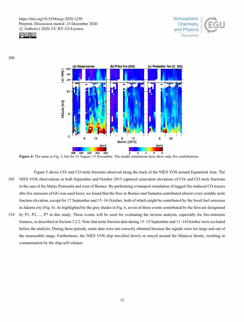
observations (Fig. 3b). A further model analysis with prior biomass burning data suggested that fire contributions to the

observed mole fraction elevations were limited mostly within the latter period of the dry season from mid-August to the

beginning of November (Fig. 4b). In the other seasons, the model showed almost no contributions from fire emissions (not

shown). In particular, the model showed a distinct fire contribution at the end of September, which elevated mole fractions up

to the upper troposphere by ~4 ppm. In the observations, although similar mole fraction elevations are found in the upper 285

troposphere, its magnitude is smaller (~2 ppm). Furthermore, the observation shows a slightly later peak that lasted until the

beginning of October (Fig. 4a). After that, the observations also captured elevated mole fraction events from mid-October

onward. However, the prior model estimate showed smaller fire contributions in October than in September (Fig. 4b), although

the simulated total CO2 mole fractions were comparable to the observations (Fig. 3b), indicating that non-fire emissions (e.g.,

from terrestrial biosphere respiration and fossil fuel emission) had a certain level of contribution during this period. 290

Figure 3: CO2 mole fractions in the free troposphere around Equatorial Asia (note that data in the boundary layer and stratosphere are excluded (see the main text)) observed by CONTRAIL (a) and their corresponding model values from prior (GG) (b) and posterior (C_GG) fluxes (c). Each upper panel presents a time-latitude cross-section from cruising mode data (~11 km above sea level) within the longitude range of 90°–130°E, and the lower one shows a time-altitude cross-section from ascending/descending data over Singapore. Note that the 295 data in the upper panels are not only from the Singapore flights but from all flights within the range. For visualisation, data are all 5-day running mean. Note also that an additional offset of 1.93 ppm is added to prior mole fractions so that the resulting global offset equals the posterior one. On the right-hand side, correlation coefficients and root-mean-square difference (RMSD) (ppm) between the simulated and observed mole fractions are noted for each time-latitude and time-altitude cross-section.


12

300

Figure 4: The same as Fig. 3, but for 15 August–15 November. The model simulations here show only fire contributions.

Figure 5 shows CO2 and CO mole fractions observed along the track of the NIES VOS around Equatorial Asia. The

NIES VOS observations in both September and October 2015 captured coincident elevations of CO2 and CO mole fractions 305

in the east of the Malay Peninsula and west of Borneo. By performing a transport simulation of tagged fire-induced CO tracers

(the fire emission of GG was used here), we found that the fires in Borneo and Sumatra contributed almost every notable mole

fraction elevation, except for 17 September and 15–16 October, both of which might be contributed by the fossil fuel emission

in Jakarta city (Fig. 6). As highlighted by the grey shades in Fig. 6, seven of those events contributed by the fires are designated

by P1, P2,…, P7 in this study. These events will be used for evaluating the inverse analysis, especially for fire-emission 310

features, as described in Section 3.2.2. Note that mole fraction data during 13–15 September and 11–14 October were excluded

before the analysis. During these periods, some data were not correctly obtained because the signals were too large and out of

the measurable range. Furthermore, the NIES VOS ship travelled slowly or stayed around the Malacca Straits, resulting in

contamination by the ship-self exhaust.


13

315 Figure 5: Mole fractions of CO2 (left) and CO (right) along the cruise tracks of NIES VOS for September (upper) and October (lower) 2015. Data enclosed by black lines with P# represent designated fire-induced high mole fraction events (see also Fig. 6).

Figure 6: Time series of CO mole fractions obtained by the in situ NIES VOS measurement (black) for September (a) and October (b) and 320 corresponding simulation results by NICAM-TM with prior CO emission data (red). Model simulations only from fire emissions in Sumatra and Borneo are also denoted by blue and cyan colours, respectively. Grey shades with P# indicate the fire-induced elevated mole fraction events.


14

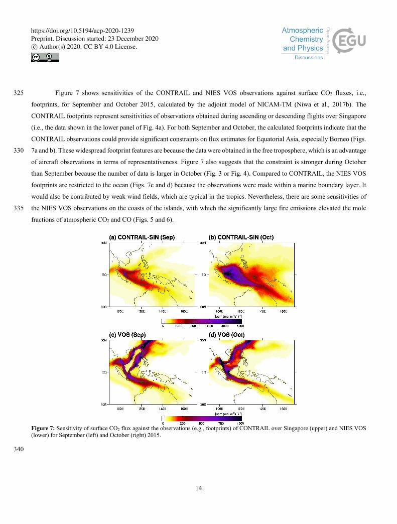
Figure 7 shows sensitivities of the CONTRAIL and NIES VOS observations against surface CO2 fluxes, i.e., 325

footprints, for September and October 2015, calculated by the adjoint model of NICAM-TM (Niwa et al., 2017b). The

CONTRAIL footprints represent sensitivities of observations obtained during ascending or descending flights over Singapore

(i.e., the data shown in the lower panel of Fig. 4a). For both September and October, the calculated footprints indicate that the

CONTRAIL observations could provide significant constraints on flux estimates for Equatorial Asia, especially Borneo (Figs.

7a and b). These widespread footprint features are because the data were obtained in the free troposphere, which is an advantage 330

of aircraft observations in terms of representativeness. Figure 7 also suggests that the constraint is stronger during October

than September because the number of data is larger in October (Fig. 3 or Fig. 4). Compared to CONTRAIL, the NIES VOS

footprints are restricted to the ocean (Figs. 7c and d) because the observations were made within a marine boundary layer. It

would also be contributed by weak wind fields, which are typical in the tropics. Nevertheless, there are some sensitivities of

the NIES VOS observations on the coasts of the islands, with which the significantly large fire emissions elevated the mole 335

fractions of atmospheric CO2 and CO (Figs. 5 and 6).

Figure 7: Sensitivity of surface CO2 flux against the observations (e.g., footprints) of CONTRAIL over Singapore (upper) and NIES VOS (lower) for September (left) and October (right) 2015.

340


15

3.2 Inversion results

3.2.1 Posterior fluxes

In this study, we investigate surface fluxes by the sum of CO2 and CO fluxes, defined as a carbon flux. We do not consider

CH4 fluxes, although they could contribute some percentage of the total carbon flux (Huijnen et al., 2016). Furthermore, we

evaluate the carbon flux separately for the total net flux and biomass burning emission. Note that the total net flux includes 345

terrestrial biosphere fluxes, biomass burnings emissions and fossil fuel emissions.

Table 3 summarises the total net and fire carbon fluxes of Equatorial Asia estimated by the five sets of inversions.

The prior biomass burning emissions of GG, GD and GS are consistently 300 Tg C for September–October, which constitutes

~80% of the annual total fire emission and amounts to more than 80% of the total net flux we prescribed as the prior (355–360

Tg C) for September–October. By inversion, all experiments, other than C_NO, estimated smaller total net fluxes by ~10% 350

(304–324 Tg C) than the priors, and they were mostly contributed by the smaller estimates of fire emissions (256–277 Tg C).

Interestingly, even when prior fire emissions were excluded in Equatorial Asia (C_NO), a significantly large fire emission of

122 Tg C was retrieved for September–October, indicating that the CONTRAIL data have fire-emission signals. However, the

estimate is half of the others, indicating some dependency of the inversion on the prior fire emissions.

355

Table 3: Total net flux and fire emission of carbon from Equatorial Asia for September–October 2015. Figure 1 defines the geographical region of Equatorial Asia. Note that the total net flux includes terrestrial biosphere fluxes, biomass burnings emissions and fossil fuel emissions. Annual flux values for 2015 are also noted in parentheses. The prior fluxes with the four biomass burning emissions are presented, as well as the posterior fluxes of the five inversions.

Total net flux [Tg C] Fire emission [Tg C] Prior (GG) 357 (677) 299 (388) Prior (GD) 360 (685) 301 (396) Prior (GS) 355 (669) 296 (379) Prior (NO) 59 (289) 0 (0) C_GG 324 (613) 277 (363) C_GD 304 (598) 256 (343) C_GS 320 (604) 265 (348) C_NO 211 (451) 122 (131) CV_GG 322 (608) 273 (362)

360

Figures 8 and 9 show the CO2 flux distributions for September and October, respectively. Here, we present the

posterior fluxes of C_GG and C_NO only, but those of the other inversions show almost similar distribution features to C_GG.

In September, C_GG estimated significantly high emissions in southeast Sumatra and south of Borneo, where the fire emission

dominated in the prior flux (Fig. 8), supporting prior knowledge of biomass burnings. However, the total emission estimate is


16

smaller than the prior by 31 Tg (Fig. 8c). In October, the differences between prior and posterior fluxes of C_GG were 365

moderate, with a net difference of 2.7 Tg (Fig. 9c). This small change in October indicates that the simulated mole fractions

from the prior flux were well consistent with the CONTRAIL observations.

Figure 8: Prior (a) and posterior (b: C_GG, e: C_NO) surface CO2 flux distributions averaged for September 2015. Difference between prior 370 and posterior fluxes (c) and prior fire emissions (d) are also shown.

Figure 9: Same as Fig. 8, but for October 2015.

375


17

As shown in Table 3, even when the fire emission was excluded from the prior, the inversion estimated notable fire

emissions (C_NO), in both September and October (Figs. 8e and 9e). Furthermore, the locations of the estimated fire emissions

are well coincident with those of prior fire emissions. They were to some extent guided by the higher prior flux errors that

were derived from the fire-emission data (the uncertainty was set as 80% of GG), which was confirmed by another sensitivity

test without prior uncertainty of fire emissions (not shown). Nevertheless, this result confirms that the CONTRAIL data have 380

information about biomass burning emissions.

Figure 10 shows temporal variations of the total net carbon flux in Equatorial Asia. Here, the posterior fluxes of

C_GG and CV_GG are shown (panel a) and the difference from each prior is presented as Δ (panel b). Note that the time series

of Δ is smoother because Δ is the parameter optimised by the inversion with a 3-day temporal correlation scale. This temporal

correlation works as a smoother. The differences between the two posterior fluxes are marginal, indicating a limited effect of 385

adding the NIES VOS data to the CONTRAIL data because the number of CONTRAIL data is overwhelming and the footprint

of CONTRAIL covers Equatorial Asia much more extensively in space (Fig. 7). Compared to the prior flux, the posterior

fluxes have a smaller peak at the beginning of September, whereas they show larger peaks from the end of September to the

beginning of October. In the latter part of October, the prior and posterior fluxes are similar.

390

Figure 10: Time series of posterior total net carbon fluxes (a) and their differences from prior (Δ) (b) for 2015. Posterior fluxes of C_GG (blue) and CV_GG (red) and their prior flux (grey) are presented.

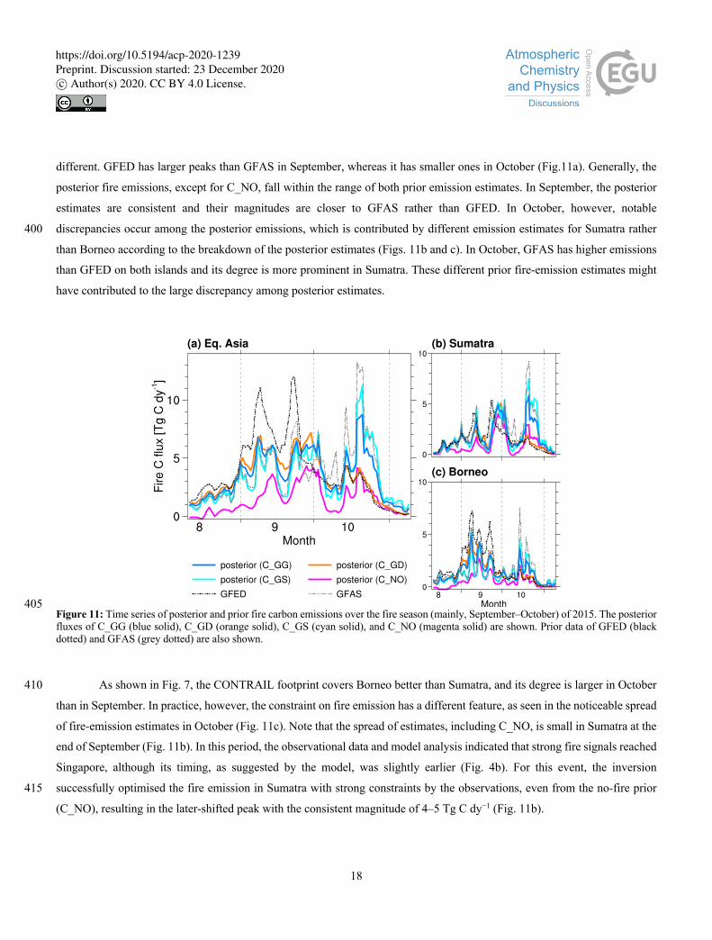
Figure 11 exhibits temporal variations of fire emissions during the fire season. In Equatorial Asia, although the timings 395

of the emission peaks presented by GFED and GFAS are coincident with each other, their magnitudes are significantly


18

different. GFED has larger peaks than GFAS in September, whereas it has smaller ones in October (Fig.11a). Generally, the

posterior fire emissions, except for C_NO, fall within the range of both prior emission estimates. In September, the posterior

estimates are consistent and their magnitudes are closer to GFAS rather than GFED. In October, however, notable

discrepancies occur among the posterior emissions, which is contributed by different emission estimates for Sumatra rather 400

than Borneo according to the breakdown of the posterior estimates (Figs. 11b and c). In October, GFAS has higher emissions

than GFED on both islands and its degree is more prominent in Sumatra. These different prior fire-emission estimates might

have contributed to the large discrepancy among posterior estimates.

405 Figure 11: Time series of posterior and prior fire carbon emissions over the fire season (mainly, September–October) of 2015. The posterior fluxes of C_GG (blue solid), C_GD (orange solid), C_GS (cyan solid), and C_NO (magenta solid) are shown. Prior data of GFED (black dotted) and GFAS (grey dotted) are also shown.

As shown in Fig. 7, the CONTRAIL footprint covers Borneo better than Sumatra, and its degree is larger in October 410

than in September. In practice, however, the constraint on fire emission has a different feature, as seen in the noticeable spread

of fire-emission estimates in October (Fig. 11c). Note that the spread of estimates, including C_NO, is small in Sumatra at the

end of September (Fig. 11b). In this period, the observational data and model analysis indicated that strong fire signals reached

Singapore, although its timing, as suggested by the model, was slightly earlier (Fig. 4b). For this event, the inversion

successfully optimised the fire emission in Sumatra with strong constraints by the observations, even from the no-fire prior 415

(C_NO), resulting in the later-shifted peak with the consistent magnitude of 4–5 Tg C dy−1 (Fig. 11b).


19

3.2.2 Posterior mole fractions

In this section, we evaluate the simulated atmospheric CO2 and CO mole fractions from the posterior fluxes. First, as shown

in Fig. 3, the posterior mole fractions of CO2 simulated for CONTRAIL have shown much better agreement with the

observations than the prior ones, demonstrating that the inverse analyses were reasonably well performed. Compared to the 420

simulation results of the prior fluxes, the posterior mole fractions have greater correlation coefficients and smaller root-mean-

square differences from the observations (see the numbers at the right-hand side of Fig. 3). In the following, we will compare

the model with the CO2 and CO observations of NIES VOS, which were left independent of the inversions, except for CV_GG.

As demonstrated by Fig. 2, the posterior CO flux includes the fire emission modified according to the modification of CO2 fire

emissions. To elucidate carbon fluxes in Equatorial Asia, the NIES VOS data used here are limited in the neighbouring region 425

(95°–125°E and 10°S–15°N).

In the comparative analysis of CO2 observations, an additional offset of 1.93 ppm is added to the prior CO2 mole

fractions so that the resulting global offset becomes equivalent to the posterior ones, i.e., ∆𝒄 of Eq. (4) is 1.93 ppm (note that

there is almost no difference in the global offset among the five inversions). Because the initial global offset was arbitrarily

given, the comparison analysis of CO2 should exclude the effect of the improvement in the global offset to better understand 430

the inversion effects.

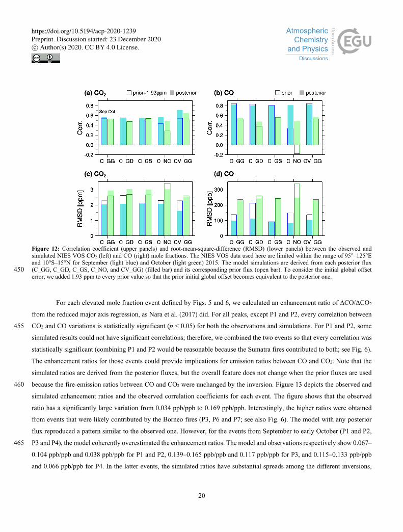
Figure 12 demonstrates how the posterior mole fractions of CO2 and CO were improved from the prior ones.

Comparing the posterior results with the prior ones, we found better consistency with the NIES VOS observation, which is

true for both CO2 and CO. Especially, its degree is notable for September; all inversions, except CV_GG, reduced the root-

mean-square difference (RMSD) of CO2 from 2.14–2.62 ppm to 2.05–2.09 ppm, whereas those of CO were reduced from 92–435

211 ppb to 80–111 ppb. These results indicate the validity of the inversions that used the CONTRAIL CO2 observations.

Especially, the experiment without the prior fire emission (C_NO) remarkably improved the correlation coefficients of CO2

and CO for both September and October (in September from 0.43 to 0.56 for CO2 and from 0.34 to 0.81 for CO, whereas in

October from 0.29 to 0.49 for CO2 and from −0.18 to 0.49 for CO); however, the other inversions, except for CV_GG, did not

improve the correlation coefficients significantly. In both months, CV_GG showed the best scores for CO2, which is 440

reasonable because it used the CO2 observations of NIES VOS. Note, however, that CV_GG used only the CO2 observations,

but not those of CO. Therefore, the RMSD reduction of CO for September by CV_GG (from 136 to 103 ppb) demonstrates

some improvement in fire emissions. Therefore, it is better to use both the CONTRAIL and NIES VOS observations for flux

estimations; however, the impact of NIES VOS is limited for the total carbon fluxes in Equatorial Asia (Table 3 and Fig. 10).

445


20

Figure 12: Correlation coefficient (upper panels) and root-mean-square-difference (RMSD) (lower panels) between the observed and simulated NIES VOS CO2 (left) and CO (right) mole fractions. The NIES VOS data used here are limited within the range of 95°–125°E and 10°S–15°N for September (light blue) and October (light green) 2015. The model simulations are derived from each posterior flux (C_GG, C_GD, C_GS, C_NO, and CV_GG) (filled bar) and its corresponding prior flux (open bar). To consider the initial global offset 450 error, we added 1.93 ppm to every prior value so that the prior initial global offset becomes equivalent to the posterior one.

For each elevated mole fraction event defined by Figs. 5 and 6, we calculated an enhancement ratio of ΔCO/ΔCO2

from the reduced major axis regression, as Nara et al. (2017) did. For all peaks, except P1 and P2, every correlation between

CO2 and CO variations is statistically significant (p < 0.05) for both the observations and simulations. For P1 and P2, some 455

simulated results could not have significant correlations; therefore, we combined the two events so that every correlation was

statistically significant (combining P1 and P2 would be reasonable because the Sumatra fires contributed to both; see Fig. 6).

The enhancement ratios for those events could provide implications for emission ratios between CO and CO2. Note that the

simulated ratios are derived from the posterior fluxes, but the overall feature does not change when the prior fluxes are used

because the fire-emission ratios between CO and CO2 were unchanged by the inversion. Figure 13 depicts the observed and 460

simulated enhancement ratios and the observed correlation coefficients for each event. The figure shows that the observed

ratio has a significantly large variation from 0.034 ppb/ppb to 0.169 ppb/ppb. Interestingly, the higher ratios were obtained

from events that were likely contributed by the Borneo fires (P3, P6 and P7; see also Fig. 6). The model with any posterior

flux reproduced a pattern similar to the observed one. However, for the events from September to early October (P1 and P2,

P3 and P4), the model coherently overestimated the enhancement ratios. The model and observations respectively show 0.067–465

0.104 ppb/ppb and 0.038 ppb/ppb for P1 and P2, 0.139–0.165 ppb/ppb and 0.117 ppb/ppb for P3, and 0.115–0.133 ppb/ppb

and 0.066 ppb/ppb for P4. In the latter events, the simulated ratios have substantial spreads among the different inversions,


21

especially for P6 (0.080–0.145 ppb/ppb) and P7 (0.123–0.182 ppb/ppb), and the observed ratios are almost at the highest level

of the simulated spreads. A further discussion is made in the following section.

470

Figure 13: Observed and simulated enhancement ratios of ΔCO/ΔCO2 (solid line) and observed correlation coefficients between ΔCO and ΔCO2 (grey bar) for each elevated mole fraction event defined by Figs. 5 and 6. The observed enhancement ratios are coloured in black. The simulated values were derived from posterior CO and CO2 fluxes of C_GG (magenta), C_GD (red), C_GS (blue), C_NO (green), and CV_GG (cyan). 475

4. Discussion

In this study, we extensively used the aircraft observations from CONTRAIL to constrain carbon fluxes in Equatorial Asia,

focusing on the devastating fire event in 2015. With the help of NIES VOS observations, especially its CO data, we have

demonstrated the validity of our inverse analysis. The estimates of biomass burning emissions are moderately smaller than the 480

prescribed datasets of GFED and GFAS. Our conceivably best estimate of CV_GG, which used both the CONTRAIL and

NIES VOS data, amounts to 273 Tg C and 362 Tg C for fire-induced carbon emissions during September–October and all

months in 2015, respectively. These numbers are in better agreement with previous top-down estimates of Huijnen et al. (2016)

(227 Tg C for September–October, and 289 Tg C for the annual total) and Heymann al. (2017) (204 Tg C for July–November)

than that of Yin et al. (2016) (510 Tg C for the annual total). Furthermore, the fire-induced carbon emission of 273 Tg C for 485

September–October is also consistent with an aerosol-based study of Kiely et al. (2019), the best estimate of which is 247 Tg

C as the sum of CO2 and CO emissions for Equatorial Asia but not including eastern areas (e.g., Papua New Guinea).


22

This study used high-precision in situ observations of CO2 to estimate carbon fluxes in contrast to studies that used

satellite observations of CO (Huijnen et al., 2016; Yin et al., 2016). Therefore, we obtained the total net carbon flux that

included biomass burning emission, terrestrial biosphere photosynthesis and respiration, and fossil fuel emission. The 490

estimated total net carbon flux amounts to 322 Tg C for September–October (CV_GG), 85% of which is contributed by fire

emissions (Table 3), indicating that flux variations of terrestrial photosynthesis and respiration under severe drought were not

as large as those of the biomass burning emissions in 2015. This result indicates that biomass burning emission is the main

driving force of interannual variations of carbon fluxes in Equatorial Asia, which is a unique feature of the carbon flux in this

region, compared with other tropical regions. Carbon fluxes in the tropics are considered to have significant sensitivities to 495

climate variations, especially to El Niño, with major driving forces of terrestrial biosphere flux changes in response to

temperature and precipitation changes (Yang and Wang, 2000; Zeng et al., 2005; Wang et al., 2013).

As described in Section 2.2, we used the common scaling factor for CO2 and CO fire fluxes; therefore, the ratio of

the emission factors (CO/CO2) was fixed to that of prior fire-emission data (GFED and GFAS) and burned carbon mass was

modified by the inverse analysis. It is likely that the spatial pattern of fire-emission ratios was reasonably represented because 500

the model reproduced the observed variation in the enhancement ratio that might be caused by the difference in their origins

(Figs. 6 and 13). However, as shown in Fig. 13, the model overestimated the enhancement ratios from September to early

October, irrespective of its origin (Borneo or Sumatra). Meanwhile, it was not the case for the latter period, although the

simulated ranges were large, indicating that the temporal change of the fire-emission ratio, i.e., a decrease of combustion

efficiency, might not be well represented in the fire-emission data. Typical fire-emission ratios of CO/CO2 are 0.2–0.3 mol/mol 505

for peatlands and 0.1 mol/mol for tropical forests, respectively (Akagi et al., 2011; Huijnen et al. 2016; Stockwell et al., 2016).

Therefore, the observed smaller enhancement ratio infers that the contribution of fires (or smouldering) in dried peatlands was

smaller in the early fire period than expected. This might have partially resulted in the smaller-than-prior estimates of the fire-

induced carbon emission (Table 3) because peatlands have high carbon density and are dominant sources of carbon (Page et

al., 2002). Nevertheless, the uncertainty is high, as demonstrated by the model large spreads, especially for the latter period, 510

and we need more observations for robust estimations of the fire-emission ratio.

We noted that the inverse analysis of this study has several limitations. First, we employed only CO2 observations in

the inverse analysis, which does not allow us to distinguish biomass burnings from other terrestrial fluxes. To separate fire-

induced and other terrestrial fluxes, it would be helpful to incorporate CO observations simultaneously with CO2 observations

into the inverse analysis; however, the availability of in situ CO observations (Novelli et al., 2003) is limited, especially for 515

Equatorial Asia. A joint CO2–CO inversion is left for a future study.

The second limitation is the dependency of the inverse analysis results on the prior estimate. We found that our inverse

calculations had a significant sensitivity to prior fire-emission data. The posterior fluxes were similar when GFED or GFAS

data were used as the prior. However, when the prior fire emissions were excluded (i.e., C_NO), the posterior flux had much

lower values, indicating that we cannot fully constrain the fluxes with CONTRAIL alone and that prior fire-emission data 520

should be as accurate as possible. The relatively small sensitivity to the difference between GFED and GFAS was because the


23

original GFED and GFAS data are comparable. Nevertheless, the well-constrained flux at the end of September in Sumatra

(Fig. 11) tells us that we could obtain a sufficient constraint from CONTRAIL when the time and location of the observations

coincide with the timing of airflow rich in emission signals. Such an airflow dependency could be reduced by making the

observations denser in space and time. To this end, the CONTRAIL project continues effort to reduce chances of missing data. 525

Finally, model transport errors would be the third limitation. Figures 3 and 4 show that even after the inversion, the

model could not sufficiently reproduce high mole fractions near the surface, suggesting some limitation of the model.

Compared to the wind data obtained from the CONTRAIL aircraft, the speed and direction of winds over Singapore were well

simulated in the model (not shown). Therefore, representative errors that include both model transport and fluxes could be one

cause. A higher resolution model is desirable, and is left for a future study with advanced computational resources. 530

In this study, we tried a regionally focused inversion using different flux parameter settings for Equatorial Asia and

the rest of the world (Table 1), which gave a sufficient degree of freedom to fluxes in Equatorial Asia, while strongly

constraining fluxes to the prior ones in the rest of the world. This inversion approach would be acceptable only when prior

fluxes can produce comparable spatiotemporal variations of atmospheric CO2 with observations, which was confirmed using

the previous inversion flux of Niwa et al. (2012). Furthermore, Niwa et al. (2012) found that CONTRAIL data could 535

independently constrain the fluxes in Equatorial Asia itself, supporting the validity of separating fluxes in Equatorial Asia from

those in the other regions. Nevertheless, the inversion flux used as the prior in this study was optimised for the different years,

which introduced a certain level of uncertainty. In future analysis, an effort for reducing uncertainties will be made by

performing a global inverse analysis by combining ground-based stations and CONTRAIL data.

5. Conclusions 540

In this study, an inverse system was developed to estimate high-spatiotemporal resolution fluxes in a focused area and

incorporate CO as a proxy for combustion sources. We performed the inverse analysis for carbon fluxes in Equatorial Asia

during the historic El Niño of 2015.

In contrast to many studies that used aircraft data for evaluating inversion results as independent data (e.g., Chevallier

et al. 2019), we extensively used the CONTRAIL aircraft data in the inverse analysis and demonstrated that the aircraft data 545

could constrain flux estimates efficiently. It is essential for Equatorial Asia because there are insufficient ground-based

observations in the region. Furthermore, the upward airflow, which is typical in the tropics, makes it difficult for remote

ground-based stations to capture flux signals (Niwa et al., 2012).

We estimated the fire-induced carbon flux to be 273 Tg C for September–October. This number accounts for 75% of

the annual fire emission and 45% of the annual net carbon flux in Equatorial Asia, demonstrating that fire emission is a major 550

driving force of the carbon flux in the region. Although the inversions have a certain degree of sensitivity to prior fire-emission

data, they coherently estimated smaller amounts than the prescribed biomass burning data. One cause could be that peatland

fires were not as severe in 2015 as expected, as suggested by the model overestimation of the enhancement ratios ΔCO/ΔCO2

captured by the NIES VOS observation. Nevertheless, this study is compatible with previous studies because a significantly


24

smaller amount of carbon was released in 2015 than in 1997, of which the El Niño intensity was comparable to that of 2015. 555

This could be because the intensity of land-use change has decreased in recent decades (Kondo et al., 2018). Another possible

underlying mechanism is the difference in precipitation patterns and amounts between 2015 and 1997 (Fanin and van der Werf,

2017). However, further investigation is needed by combining process-based terrestrial biosphere models, biomass burning

emission models and inverse estimates, as in this study.

Although it is smaller than 1997, our estimate of the fire-induced emissions in 2015 is still notably high. Field et al. 560

(2016) pointed out that the fire emissions estimated by GFED for Equatorial Asia in 2015 are higher than the annual fossil fuel

emissions of Japan. Our estimate is smaller than that of GFED, but still comparable to the latest Japanese inventory (338 TgC

yr−1 for 2018 (GIO and MOE, 2020)). Using an atmospheric climate model, Shiogama et al. (2020) projected that Equatorial

Asia would experience stronger droughts than that in 2015 in a future warmer climate condition. To reduce fire-induced carbon

emissions from such drought events, chances of ignition must be reduced. The continuous monitoring of carbon emissions 565

with high-precision atmospheric observations is indispensable for mitigation measures against fires. The ongoing activity of

aircraft- and ship-based observations used in this study will continue to provide practical implications and reliable quantitative

estimates of carbon emissions from Equatorial Asia along with an inverse analysis.

Data Availability 570

The CO2 mole fraction data of CONTRAIL (Machida et al., 2018) and NIES VOS used in this study are available from the

Global Environmental Database (GED) of NIES (http://db.cger.nies.go.jp/portal/geds/atmosphericAndOceanicMonitoring).

The CO observational data of NIES VOS are available on request to H. Nara.

Author Contributions 575

YN designed and conducted the inversion analyses. TM, YS, HM, YN and TU conducted the CONTRAIL observations and

HN, SN, HT and YT conducted the NIES VOS observations. AI provided the VISIT data. YN prepared the manuscript with

contributions from all co-authors.

Competing Interest

The authors declare that they have no conflict of interest. 580

Acknowledgements


25

This study was supported mainly by the Environment Research and Technology Development Fund of the Ministry of the

Environment, Japan, and the Environmental Restoration and Conservation Agency of Japan (JPMEERF20142001 and

JPMEERF20172001), whose project leader was Nobuko Saigusa of NIES. The work was also supported by the JSPS

KAKENHI, Grant Number 19K03976. The inverse simulations in this study were performed on the NIES supercomputer 585

system (NEC SX-ACE). The observations from the CONTRAIL project are conducted under great supports of Japan Airlines,

JAMCO and the JAL Foundation. The observational projects of CONTRAIL and NIES VOS are financially supported by the

research fund by Global Environmental Research Coordination System of the Ministry of the Environment, Japan (E1253,

E1652, E1851). YN is grateful to the NICAM developers of the University of Tokyo, JAMSTEC, RIKEN and NIES for

maintaining and developing NICAM. Our appreciation is also extended to Tomoko Shirai and Yoko Fukuda of NIES for 590

developing and maintaining GED, through which we make our observational data publicly available.

References

Akagi, S. K., Yokelson, R. J., Wiedinmyer, C., Alvarado, M. J., Reid, J. S., Karl, T., Crounse, J. D., and Wennberg, P. O.:

Emission factors for open and domestic biomass burning for use in atmospheric models, Atoms. Chem. Phys., 11, 4039–595

4072, https://doi.org/10.5194/acp-11-4039-2011, 2011.

Andres, R. J., Boden, T., and Marland, G.: Monthly Fossil-Fuel CO2 Emissions: Mass of Emissions Gridded by One Degree

Latitude by One Degree Longitude, Carbon Dioxide Information Analysis Center, Oak Ridge National Laboratory, U.S.

Department of Energy, Oak Ridge, Tenn., U.S.A., https://doi.org/10.3334/CDIAC/ffe.MonthlyMass.2016, 2016.

Baker, D. F., Law, R. M., Gurney, K. R., Rayner, P., Peylin, P., Denning, A. S., Bousquet, P., Bruhwiler, L., Chen, Y., Ciais, 600

P., Fung, I. Y., Heimann, M., John, J., Maki, T., Maksyutov, S., Masarie, K., Prather, M., Pak, B., Taguchi, S., and Zhu,

Z.: TransCom 3 inversion intercomparison: Impact of transport model errors on the interannual variability of regional CO2

fluxes, 1988–2003, Global Biogeochem. Cycles, 20, https://doi.org/10.1029/2004GB002439, 2006.

Chevallier, F., Ciais, P., Conway, T. J., Aalto, T., Anderson, B. E., Bousquet, P., Brunke, E. G., Ciattaglia, L., Esaki, Y.,

Fröhlich, M., Gomez, A., Gomez-Pelaez, A. J., Haszpra, L., Krummel, P. B., Langenfelds, R. L., Leuenberger, M., 605

Machida, T., Maignan, F., Matsueda, H., Morguí, J. A., Mukai, H., Nakazawa, T., Peylin, P., Ramonet, M., Rivier, L.,

Sawa, Y., Schmidt, M., Steele, L. P., Vay, S. A., Vermeulen, A. T., Wofsy, S., and Worthy, D.: CO2 surface fluxes at grid

point scale estimated from a global 21 year reanalysis of atmospheric measurements, J. Geophys. Res., 115,

https://doi.org/10.1029/2010JD013887, 2010.


26

Chevallier, F., Remaud, M., O’Dell, C. W., Baker, D., Peylin, P., and Cozic, A.: Objective evaluation of surface- and satellite-610

driven carbon dioxide atmospheric inversions, Atoms. Chem. Phys., 19, 14 233–14 251, https://doi.org/10.5194/acp-19-

14233-2019, 2019.

Crisp, D.: NASA Orbiting Carbon Observatory: measuring the column averaged carbon dioxide mole fraction from space, J.

Appl. Remote Sens., 2, 023 508, https://doi.org/10.1117/1.2898457, 2008.

Crisp, D.: Measuring atmospheric carbon dioxide from space with the Orbiting Carbon Observatory-2 (OCO-2), in: Earth 615

Observ. Syst. XX, SPIE, https://doi.org/10.1117/12.2187291, 2015.

Enting, I. G.: Inverse Problems in Atmospheric Constituent Transport, Cambridge University Press, New York, 2002.

Fanin, T., and van der Werf, G. R.: Precipitation–fire linkages in Indonesia (1997–2015), Biogeosciences, 14, 3995–4008,

https://doi.org/10.5194/bg-14-3995-2017, 2017.

Field, R., van der Werf, G., Fanin, T., Fetzer, E., Fuller, R., Jethva, H., Levy, R., Livesey, N., Luo, M., Torres, O., and Worden, 620

H.: Indonesian fire activity and smoke pollution in 2015 show persistent nonlinear sensitivity to El Niño-induced drought,

Proc. Natl. Acad. Sci. (USA), 113, 9204–9209, https://doi.org/10.1073/pnas.1524888113, 2016.

Field, R. D., van der Werf, G. R., and Shen, S. S. P.: Human amplification of drought-induced biomass burning in Indonesia

since 1960, Nature Geoscience, 2, 185–188, https://doi.org/10.1038/ngeo443, 2009.

Fujii, Y.: Preconditioned Optimizing Utility for Large-dimensional analyses (POpULar), J. Oceanogr., 61, 167–181, 625

https://doi.org/10.1007/s10872-005-0029-z, 2005.

Fujii, Y., and Kamachi, M.: A nonlinear preconditioned quasi-Newton method without inversion of a first-guess covariance

matrix in variational analyses, Tellus A, 55, 450–454, https://doi.org/10.1034/j.1600-0870.2003.00030.x, 2003.

Giglio, L., Randerson, J. T., and van der Werf, G. R.: Analysis of daily, monthly, and annual burned area using the fourth-

generation global fire emissions database (GFED4), J. Geophys. Res., 118, 317–328, https://doi.org/10.1002/jgrg.20042, 630

2013.

Greenhouse Gas Inventory Office of Japan (GIO) and Ministry of the Environment, Japan (MOE) (eds.): National Greenhouse

Gas Inventory Report of JAPAN 2020, Center for Global Environmental Research, National Institute for Environmental

Studies, Japan, 2002.

Harada, Y., Kamahori, H., Kobayashi, C., Endo, H., Kobayashi, S., Ota, Y., Onoda, H., Onogi, K., Miyaoka, K., and Takahashi, 635

K.: The JRA-55 reanalysis: representation of atmospheric circulation and climate variability, J. Meteor. Soc. Japan, 94,

269–302, https://doi.org/10.2151/jmsj.2016-015, 2016.

Heymann, J., Reuter, M., Buchwitz, M., Schneising, O., Bovensmann, H., Burrows, J. P., Massart, S., Kaiser, J. W., and Crisp,

D.: CO2 emission of Indonesian fires in 2015 estimated from satellite-derived atmospheric CO2 concentrations, Geophys.

Res. Lett., 44, 1537– 1544, https://doi.org/10.1002/2016gl072042, 2017. 640

Huijnen, V., Wooster, M. J., Kaiser, J. W., Gaveau, D. L. A., Flemming, J., Parrington, M., Inness, A., Murdiyarso, D., Main,

B., and van Weele, M.: Fire carbon emissions over maritime southeast Asia in 2015 largest since 1997, Sci. Rep., 6,

https://doi.org/10.1038/srep26886, 2016.


27

Iida, Y., Kojima, A., Takatani, Y., Nakano, T., Sugimoto, H., Midorikawa, T., and Ishii, M.: Trends in pCO2 and sea–air CO2

flux over the global open oceans for the last two decades, J. Oceanogr., 71, https://doi.org/10.1007/s10872-015-0306-4, 645

2015.

Ito, A.: Disequilibrium of terrestrial ecosystem CO2 budget caused by disturbance-induced emissions and non-CO2 carbon

export flows: a global model assessment, Earth Syst. Dyn., 10, 685–709, https://doi.org/10.5194/esd-10-685-2019, 2019.

Ito, A., and Inatomi, M.: Use of a process-based model for assessing the methane budgets of global terrestrial ecosystems and

evaluation of uncertainty, Biogeosciences, 9, 759–773, https://doi.org/10.5194/bg-9-759-2012, 2012. 650

Janssens-Maenhout, G., Crippa, M., Guizzardi, D., Muntean, M., Schaaf, E., Dentener, F., Bergamaschi, P., Pagliari, V.,

Olivier, J. G. J., Peters, J. A. H. W., van Aardenne, J. A., Monni, S., Doering, U., Petrescu, A. M. R., Solazzo, E., and

Oreggioni, G. D.: EDGAR v4.3.2 Global Atlas of the three major greenhouse gas emissions for the period 1970–2012,

Earth Syst. Sci. Data, 11, 959–1002, https://doi.org/10.5194/essd-11-959-2019, 2019.

Kaiser, J. W., Heil, A., Andreae, M. O., Benedetti, A., Chubarova, N., Jones, L., Morcrette, J.-J., Razinger, M., Schultz, M. 655

G., Suttie, M., and van der Werf, G. R.: Biomass burning emissions estimated with a global fire assimilation system based

on observed fire radiative power, Biogeosciences, 9, 527–554, https://doi.org/10.5194/bg-9-527-2012, 2012.

Kiely, L., Spracklen, D. V., Wiedinmyer, C., Conibear, L., Reddington, C. L., Archer-Nicholls, S., Lowe, D., Arnold, S. R.,

Knote, C., Khan, M. F., Latif, M. T., Kuwata, M., Budisulistiorini, S. H., and Syaufina, L.: New estimate of particulate

emissions from Indonesian peat fires in 2015, Atmos. Chem. Phys., 19, 11105–11121, https://doi.org/10.5194/acp-19-660

11105-2019, 2019.

Kobayashi, S., Ota, Y., Harada, Y., Ebita, A., Moriya, M., Onoda, H., Onogi, K., Kamahori, H., Kobayashi, C., Endo, H.,

Miyaoka, K., and Takahashi, K.: The JRA-55 Reanalysis: General Specifications and Basic Characteristics, J. Meteor.

Soc. Japan, 93, 5–48, https://doi.org/10.2151/jmsj.2015-001, 2015.

Kondo, M., Ichii, K., Patra, P. K., Canadell, J. G., Poulter, B., Sitch, S., Calle, L., Liu, Y. Y., van Dijk, A. I. J. M., Saeki, T., 665

Saigusa, N., Friedlingstein, P., Arneth, A., Harper, A., Jain, A. K., Kato, E., Koven, C., Li, F., Pugh, T. A. M., Zaehle, S.,

Wiltshire, A., Chevallier, F., Maki, T., Nakamura, T., Niwa, Y., and Rödenbeck, C.: Land use change and El Niño-

Southern Oscillation drive decadal carbon balance shifts in Southeast Asia, Nature Comm., 9,

https://doi.org/10.1038/s41467-018-03374-x, 2018.

L’Heureux, M. L., Takahashi, K., Watkins, A. B., Barnston, A. G., Becker, E. J., Liberto, T. E. D., Gamble, F., Gottschalck, 670

J., Halpert, M. S., Huang, B., Mosquera-Vásquez, K., and Wittenberg, A. T.: Observing and Predicting the 2015/16 El

Niño, Bull. Amer. Meteor. Soc., 98, 1363–1382, https://doi.org/10.1175/bams-d-16-0009.1, 2017.

Machida, T., Matsueda, H., Sawa, Y., Nakagawa, Y., Hirotani, K., Kondo, N., Goto, K., Nakazawa, T., Ishikawa, K., and

Ogawa, T.: World- wide measurements of atmospheric CO2 and other trace gas species using commercial airlines, J.

Atmos. Oceanic Technol., 25, 1744–1754, https://doi.org/10.1175/2008JTECHA1082.1, 2008. 675


28

Machida, T., K. Ishijima, Y. Niwa, K. Tsuboi, Y. Sawa and H. Matsueda (2018). Atmospheric CO2 mole fraction data of

CONTRAIL-CME, Ver.2019.1.0, Center for Global Environmental Research. NIES,

https://doi.org/10.17595/20180208.001 (Reference date: 2019/03/05)

Matsueda, H., and Inoue, H. Y.: Aircraft measurements of trace gases between Japan and Singapore in October of 1993, 1996,

and 1997, Geophys. Res. Lett., 26, 2413–2416, https://doi.org/10.1029/1999GL900089, 1999. 680

Matsueda, H., Inoue, H. Y., and Ishii, M.: Aircraft observation of carbon dioxide at 8–13 km altitude over the western Pacific

from 1993 to 1999, Tellus B, 54, 1–21, https://doi.org/10.1034/j.1600-0889.2002.00304.x, 2002.

Matsueda, H., Buchholz, R. R., Ishijima, K., Worden, H. M., Hammerling, D., and Machida, T.: Interannual Variation of

Upper Tropospheric CO over the Western Pacific Linked with Indonesian Fires, SOLA, 15, 205–210,

https://doi.org/10.2151/sola.2019-037, 2019. 685

Mu, M., Randerson, J. T., van der Werf, G. R., Giglio, L., Kasibhatla, P., Morton, D., Collatz, G. J., DeFries, R. S., Hyer, E.

J., Prins, E. M., Griffith, D. W. T., Wunch, D., Toon, G. C., Sherlock, V., and Wennberg, P. O.: Daily and 3-hourly

variability in global fire emissions and consequences for atmospheric model predictions of carbon monoxide, J. Geophys.

Res., 116, https://doi.org/10.1029/2011JD016245, 2011.

Nakaoka, S., Telszewski, M., Nojiri, Y., Yasunaka, S., Miyazaki, C., Mukai, H., and Usui, N.: Estimating temporal and spatial 690

variation of ocean surface pCO2 in the North Pacific using a self-organizing map neural network technique,

Biogeosciences, 10, 6093–6106, https://doi.org/10.5194/bg-10-6093-2013, 2013.

Nara, H., Tanimoto, H., Nojiri, Y., Mukai, H., Machida, T., and Tohjima, Y.: Onboard measurement system of atmospheric

carbon monoxide in the Pacific by voluntary observing ships, Atoms. Meas. Tech., 4, 2495–2507,

https://doi.org/10.5194/amt-4-2495-2011, 2011. 695

Nara, H., Tanimoto, H., Tohjima, Y., Mukai, H., Nojiri, Y., and Machida, T.: Emissions of methane from offshore oil and gas

platforms in Southeast Asia, Scientific Reports, 4, https://doi.org/10.1038/srep06503, 2014.

Nara, H., Tanimoto, H., Tohjima, Y., Mukai, H., Nojiri, Y., and Machida, T.: Emission factors of CO2, CO and CH4 from

Sumatran peatland fires in 2013 based on shipboard measurements, Tellus B, 69, 1399 047,

https://doi.org/10.1080/16000889.2017.1399047, 2017. 700

Niwa, Y., Patra, P. K., Sawa, Y., Machida, T., Matsueda, H., Belikov, D., Maki, T., Ikegami, M., Imasu, R., Maksyutov, S.,

Oda, T., Satoh, M., and Takigawa, M.: Three-dimensional variations of atmospheric CO2: aircraft measurements and

multi-transport model simulations, Atoms. Chem. Phys., 11, 13 359–13 375, https://doi.org/10.5194/acp-11-13359-2011,

2011a.

Niwa, Y., Tomita, H., Satoh, M., and Imasu, R.: A three-dimensional icosahedral grid advection scheme preserving 705

monotonicity and consistency with continuity for atmospheric tracer transport, J. Meteor. Soc. Japan, 89, 255–268,

https://doi.org/10.2151/jmsj.2011- 306, 2011b.


29

Niwa, Y., Machida, T., Sawa, Y., Matsueda, H., Schuck, T. J., Brenninkmeijer, C. A. M., Imasu, R., and Satoh, M.: Imposing

strong constraints on tropical terrestrial CO2 fluxes using passenger aircraft based measurements, J. Geophys. Res., 117,

https://doi.org/10.1029/2012JD017474, 2012. 710

Niwa, Y., Fujii, Y., Sawa, Y., Iida, Y., Ito, A., Satoh, M., Imasu, R., Tsuboi, K., Matsueda, H., and Saigusa, N.: A 4D-Var

inversion system based on the icosahedral grid model (NICAM-TM 4D-Var v1.0) – Part 2: Optimization scheme and

identical twin experiment of atmospheric CO2 inversion, Geosci. Model Dev., 10, 2201–2219,

https://doi.org/10.5194/gmd-10-2201-2017, 2017a.

Niwa, Y., Tomita, H., Satoh, M., Imasu, R., Sawa, Y., Tsuboi, K., Matsueda, H., Machida, T., Sasakawa, M., Belan, B., and 715

Saigusa, N.: A 4D-Var inversion system based on the icosahedral grid model (NICAM-TM 4D-Var v1.0) – Part 1: Offline

forward and adjoint transport models, Geosci. Model Dev., 10, 1157–1174, https://doi.org/10.5194/gmd-10-1157-2017,

2017b.

Novelli, P. C., Masarie, K. A., Lang, P. M., Hall, B. D., Myers, R. C., and Elkins, J. W.: Reanalysis of tropospheric CO trends:

Effects of the 1997–1998 wildfires, J. Geophys. Res., 108, https://doi.org/10.1029/2002JD003031, 2003. 720

Olsen, S. C., and Randerson, J. T.: Differences between surface and column atmospheric CO2 and implications for carbon

cycle research, J. Geophys. Res., 109, https://doi.org/10.1029/2003JD003968, 2004.

Page, S. E., Siegert, F., Rieley, J. O., Boehm, H.-D. V., Jaya, A., and Limin, S.: The amount of carbon released from peat and

forest fires in Indonesia during 1997, Nature, 420, 61–65, https://doi.org/10.1038/nature01131, 2002.

Page, S. E., Rieley, J. O., and Banks, C. J.: Global and regional importance of the tropical peatland carbon pool, Global Change 725

Biology, 17, 798–818, https://doi.org/10.1111/j.1365-2486.2010.02279.x, 2011.

Patra, P. K., Ishizawa, M., Maksyutov, S., Nakazawa, T., and Inoue, G.: Role of biomass burning and climate anomalies for

land-atmosphere carbon fluxes based on inverse modeling of atmospheric CO2, Global Biogeochem. Cycles, 19,

https://doi.org/10.1029/2004GB002258, 2005.

Patra, P. K., Houweling, S., Krol, M., Bousquet, P., Belikov, D., Bergmann, D., Bian, H., Cameron-Smith, P., Chipperfield, 730

M. P., Corbin, K., Fortems-Cheiney, A., Fraser, A., Gloor, E., Hess, P., Ito, A., Kawa, S. R., Law, R. M., Loh, Z.,

Maksyutov, S., Meng, L., Palmer, P. I., Prinn, R. G., Rigby, M., Saito, R., and Wilson, C.: TransCom model simulations

of CH4 and related species: linking transport, surface flux and chemical loss with CH4 variability in the troposphere and

lower stratosphere, Atoms. Chem. Phys., 11, 12 813–12 837, https://doi.org/10.5194/acp-11-12813-2011, 2011.

Randerson, J. T., Thompson, M. V., Conway, T. J., Fung, I. Y., and Field, C. B.: The contribution of terrestrial sources and 735

sinks to trends in the seasonal cycle of atmospheric carbon dioxide, Global Biogeochem. Cycles, 11, 535–560,

https://doi.org/10.1029/97GB02268, 1997.

Randerson, J. T., Chen, Y., van der Werf, G. R., Rogers, B. M., and Morton, D. C.: Global burned area and biomass burning

emissions from small fires, J. Geophys. Res., 117, https://doi.org/10.1029/2012JG002128, 2012.

Rayner, P. J., Enting, I. G., and Trudinger, C. M.: Optimizing the CO2 observing network for constraining sources and sinks, 740

Tellus B, 48, 433–444, https://doi.org/10.3402/tellusb.v48i4.15924, 1996.


30

Rödenbeck, C.: Estimating CO2 sources and sinks from atmospheric mixing ratio measurements using a global inversion of

atmospheric transport, Max-Planck-Institut für Biogeochemie: Technical Paper 6, 2005.

Santoso, A., Mcphaden, M. J., and Cai, W.: The Defining Characteristics of ENSO Extremes and the Strong 2015/2016 El

Niño, Reviews of Geophysics, 55, 1079–1129, https://doi.org/10.1002/2017rg000560, 2017. 745

Satoh, M., Matsuno, T., Tomita, H., Miura, H., Nasuno, T., and Iga, S.: Nonhydrostatic icosahedral atmospheric model

(NICAM) for global cloud resolving simulations, J. Comput. Phys., 227, 3486–3514,

https://doi.org/10.1016/j.jcp.2007.02.006, 2008.

Satoh, M., Tomita, H., Yashiro, H., Miura, H., Kodama, C., Seiki, T., Noda, A. T., Yamada, Y., Goto, D., Sawada, M., Miyoshi,

T., Niwa, Y., Hara, M., Ohno, T., Iga, S., Arakawa, T., Inoue, T., and Kubokawa, H.: The Non-hydrostatic Icosahedral 750

Atmospheric Model: description and development, Progress in Earth and Planetary Science, 1, 1–32,

https://doi.org/10.1186/s40645-014-0018-1, 2014.

Sawa, Y., Matsueda, H., Tsutsumi, Y., Jensen, J. B., Inoue, H. Y., and Makino, Y.: Tropospheric carbon monoxide and

hydrogen measurements over Kalimantan in Indonesia and northern Australia during October 1997, Geophys. Res. Lett.,

26, 1389–1392, https://doi.org/10.1029/1999GL900247, 1999. 755

Sawa, Y., Machida, T., and Matsueda, H.: Seasonal variations of CO2 near the tropopause observed by commercial aircraft, J.

Geophys. Res., 113, https://doi.org/10.1029/2008jd010568, 2008.

Sawa, Y., Machida, T., and Matsueda, H.: Aircraft observation of the seasonal variation in the transport of CO2 in the upper

atmosphere, J. Geophys. Res., 117, https://doi.org/10.1029/2011jd016933, 2012.

Shiogama, H., Hirata, R., Hasegawa, T., Fujimori, S., Ishizaki, N. N., Chatani, S., Watanabe, M., Mitchell, D., and Lo, Y. T. 760

E.: Historical and future anthropogenic warming effects on droughts, fires and fire emissions of CO2 and PM2.5 in

equatorial Asia when 2015-like El Niño events occur, Earth System Dynamics, 11, 435–445, https://doi.org/10.5194/esd-

11-435-2020, 2020.

Stockwell, C. E., Yokelson, R. J., Kreidenweis, S. M., Robinson, A. L., DeMott, P. J., Sullivan, R. C., Reardon, J., Ryan, K.

C., Griffith, D. W. T., and Stevens, L.: Trace gas emissions from combustion of peat, crop residue, domestic biofuels, 765

grasses, and other fuels: configuration and Fourier transform infrared (FTIR) component of the fourth Fire Lab at Missoula

Experiment (FLAME-4), Atoms. Chem. Phys., 14, 9727–9754, https://doi.org/10.5194/acp-14-9727-2014, 2014.

Takatani, Y., Enyo, K., Iida, Y., Kojima, A., Nakano, T., Sasano, D., Kosugi, N., Midorikawa, T., Suzuki, T., and Ishii, M.:

Relationships between total alkalinity in surface water and sea surface dynamic height in the Pacific Ocean, J. Geophys.

Res., 119, 2806–2814, https://doi.org/10.1002/2013jc009739, 2014. 770

Terao, Y., Mukai, H., Nojiri, Y., Machida, T., Tohjima, Y., Saeki, T., and Maksyutov, S.: Interannual variability and trends in

atmospheric methane over the western Pacific from 1994 to 2010, J. Geophys. Res., 116,

https://doi.org/10.1029/2010jd015467, 2011.

Tohjima, Y., Mukai, H., Machida, T., Nojiri, Y., and Gloor, M.: First measurements of the latitudinal atmospheric O2 and CO2

distributions across the western Pacific, Geophys. Res. Lett., 32, https://doi.org/10.1029/2005GL023311, 2005. 775


31

Tomita, H., and Satoh, M.: A new dynamical framework of nonhydrostatic global model using the icosahedral grid, Fluid Dyn.

Res., 34, 357–400, https://doi.org/10.1016/j.fluiddyn.2004.03.003, 2004.

Umezawa, T., Matsueda, H., Sawa, Y., Niwa, Y., Machida, T., and Zhou, L.: Seasonal evaluation of tropospheric CO2 over

the Asia-Pacific region observed by the CONTRAIL commercial airliner measurements, Atoms. Chem. Phys., 18, 14851–

14866, https://doi.org/10.5194/acp-18-14851-2018, 2018. 780

Umezawa, T., Matsueda, H., Oda, T., Higuchi, K., Sawa, Y., Machida, T., Niwa, Y., and Maksyutov, S.: Statistical

characterization of urban CO2 emission signals observed by commercial airliner measurements, Sci. Rep., 10,

https://doi.org/10.1038/s41598-020-64769- 9, 2020.

van der Werf, G. R., Dempewolf, J., Trigg, S. N., Randerson, J. T., Kasibhatla, P. S., Giglio, L., Murdiyarso, D., Peters, W.,

Morton, D. C., Collatz, G. J., Dolman, A. J., and DeFries, R. S.: Climate regulation of fire emissions and deforestation in 785

equatorial Asia, Proc. Natl. Acad. Sci. (USA), 105, 20 350–20 355, https://doi.org/10.1073/pnas.0803375105, 2008.

van der Werf, G. R., Randerson, J. T., Giglio, L., van Leeuwen, T. T., Chen, Y., Rogers, B. M., Mu, M., van Marle, M. J. E.,

Morton, D. C., Collatz, G. J., Yokelson, R. J., and Kasibhatla, P. S.: Global fire emissions estimates during 1997–2016,

Earth Syst. Sci. Data, 9, 697–720, https://doi.org/10.5194/essd-9-697-2017, 2017.

Wang, W., Ciais, P., Nemani, R., Canadell, J., Piao, S., Sitch, S., White, M., Hashimoto, H., Milesi, C., and Myneni, R.: 790

Variations in atmospheric CO2 growth rates coupled with tropical temperature, Proc. Natl. Acad. Sci. (USA), 110, 13061–

13066, https://doi.org/10.1073/pnas.1219683110, 2013.

World Meteorological Organization (WMO) (2018). WMO Greenhouse Gas Bulletin.

Yang, X., and Wang, M.: Monsoon ecosystems control on atmospheric CO2 interannual variability: Inferred from a significant

positive correlation between year-to-year changes in land precipitation and atmospheric CO2 growth rate, Geophys. Res. 795

Lett., 27, 1671–1674, https://doi.org/10.1029/1999gl006073, 2000.

Yin, Y., Chevallier, F., Ciais, P., Broquet, G., Fortems-Cheiney, A., Pison, I., and Saunois, M.: Decadal trends in global CO

emissions as seen by MOPITT, Atoms. Chem. Phys., 15, 13 433–13 451, https://doi.org/10.5194/acp-15-13433-2015,

2015.

Yin, Y., Ciais, P., Chevallier, F., van der Werf, G. R., Fanin, T., Broquet, G., Boesch, H., Cozic, A., Hauglustaine, D., Szopa, 800

S., and Wang, Y.: Variability of fire carbon emissions in equatorial Asia and its nonlinear sensitivity to El Niño, Geophys.

Res. Lett., 43, 10,472–10,479, https://doi.org/10.1002/2016gl070971, 2016.

Zeng, N., Mariotti, A., and Wetzel, P.: Terrestrial mechanisms of interannual CO2 variability, Global Biogeochem. Cycles, 19,

https://doi.org/10.1029/2004gb002273, 2005.


Documents

0,.)0&+1'(),%$$'()*+'%)!2/&'+$&3)4$&)$() 5678)19)/$( - ACP