007-0210

Credit Risk Analysis Applying Logistic Regression, Neural Networks and Genetic

Algorithms Models

Maria Aparecida Gouvêa

University of São Paulo, Brazil

Av. Prof. Luciano Gualberto, 908 Cidade Universitária Sala – E110

ZIP CODE 05508-900 SP

e-mail: magouvea@usp.br Phone: 55 11 30916044

Eric Bacconi Gonçalves

University of São Paulo, Brazil

Av. Prof. Luciano Gualberto, 908 Cidade Universitária Sala – E110

ZIP CODE 05508-900 SP

e-mail: eric.goncalves@telefonica.com.br Phone: 55 11 30916044

POMS 18th Annual Conference

Dallas, Texas, U.S.A.

May 4 to May 7, 2007

2

ABSTRACT

Credit models are useful to evaluate the risk of consumer loans. The application of the

technique with greater precision of a prediction model will provide financial returns to the

institution. In this study a sample set of applicants from a large Brazilian financial

institution was focused on in order to develop three models each one based on one of the

alternative techniques: Logistic Regression, Neural Networks and Genetic Algorithms.

Finally, the quality and performance of these models are evaluated and compared to

identify the best one. Results obtained by the logistic regression and neural network models

are good and very similar, although the former is slightly better. The genetic algorithm

model is also efficient, but somewhat inferior. This study illustrates the procedures to be

adopted by a financial institution in order to identify the best credit model to evaluate the

risk of consumer loans and thereby get increasing profits.

Keywords: Credit risk, Logistic regression, Neural networks, Genetic algorithm.

3

1. SCENARIO

With the currency stability achieved by the Economical Plano Real in 1994, financial

loans became a good business for the banks that no longer made such large profits from

currency devaluation. (ROSA, 2000: 1). To replace this profitability, the need to increase

investment alternatives was felt at the end of the inflation period. Thereafter institutions

have endeavored to expand their credit portfolios. However, loans could not be offered at

random to all the applicant clients, therefore ways to evaluate the candidates were required.

Some years ago, when applying for a loan, the client filled in a proposal for evaluation

by one or more analysts. They then issued an opinion regarding the request (SEMOLINI,

2002: 103). Although effective, the process was slow because it did not accommodate the

analysis of many requests. As such, the model for the analysis of the concession of credit

was initially introduced in financial institutions aiming to speed up evaluation of proposals.

Models of analysis for extension of credit known as models of credit scoring are based

on historical information from the databank on existing clients, in order to assess whether

the prospective client will have a greater chance of being a good or bad payer. The models

of credit scoring are added to the institution’s systems permitting on-line credit evaluation.

1.1 Objectives of the Study

Based on the data of a sample, the intention is to:

• Develop three credit scoring models by using three statistical/computational

techniques: Logistic Regression, Neural Networks, Genetic Algorithms

4

• Compare the models developed in terms of the quality of fitness and prediction

indicators;

• Propose a model for the classification of clients

2.THEORETICAL BASIS

In this section, the theoretical concepts that will support the theme of this work will be

presented.

2.1 Consumer Credit

The expression consumer credit may be understood as a form of trade where a person

obtains money, goods or services and vouches to pay for this in the future, adding a

premium (interest) to the original value (SANTOS, 2000: 15).

Currently, consumer credit is a large industry operating worldwide. Major retailers

spur their sales by supplying credit. Automobile companies, banks and other segments

utilize consumer credit lines as an additional alternative to make profit. On the other hand,

consumer credit injects resources into the economy, permitting production and economic

expansion of a country, thereby bringing development to the nation (LEWIS, 1992: 2).

However to make credit widely available does not mean to distribute credit at random

to all those requesting it; there is a factor associated to consumer credit which is crucial in

the decision of making credit available or not: the risk.

5

2.2 Risk of Credit

On the financial market, risk of credit is the oldest form of risk (FIGUEIREDO, 2001:

9). It is the upshot of a financial transaction, contracted between the supplier of funds (giver

of credit) and the user (taker of credit). Prior to any sophistication resulting from financial

engineering, the mere act of lending a sum to someone entails the probability of it not being

repaid, the uncertainty regarding return. This is, in essence, the risk of credit which may be

defined as the risk of a counterpart, in an agreement of credit concession, not to meet

his/her obligation.

According to Caouette et al. (2000: 1), “if credit may be defined as the expectation of

receiving a sum of money in a given period, then Risk of Credit is a chance that this

expectation is not fulfilled”.

The activity of credit concession is a basic function of banks, therefore risk of credit

takes on a relevant role in the composition of an institution’s risks and may be found in the

operations where there is a transfer of money to the clients as well as in those where there is

only a possibility of usage, the pre-conceded limits. Primary types of a bank credit

operation are: loans, financing, discount of payables, advancement to depositors,

advancement of exchange, leasing operations, surety bonds and warranties etc.

In these operations risk may take on different forms; to be conceptually familiar with

them helps to orient management and mitigation.

In the universe of consumer credit, pledge of future payment involves the idea of risk.

As the future cannot be fully predicted, all consumer credit involves risk, because assurance

of payment does not exist (LEWIS, 1992: 2). Analysis of credit is charged with the task of

estimating the risk involved in the concession or not of credit.

6

The maximum risk that the institution may accept relies on the policy adopted by the

company. Risk presented by the applicant is of major significance for the process of credit

concession, and various queries must be considered in its evaluation.

2.3 Evaluation of the Risk of Credit

Evaluation of risk is the main issue for concession of credit. If the risk is poorly

evaluated the company will certainly lose money, be it because of acceptance of clients

who will generate losses to the business or because of the refusal of good clients who

would generate profits for the business. Companies who have a better evaluation than their

competitors in the concession of credit have an advantage over the others as they are less

vulnerable to the consequence of the wrong decisions when providing credit.

Evaluation of risk of a potential client can be carried out in two ways:

1. By judgment, a more subjective way involving a more qualitative analysis;

2. By classifying the taker by means of evaluation models, involving a more

quantitative analysis.

Currently, almost all large sized companies working with concession of credit use a

combination of both.

The models called credit scoring are used for the evaluation of risk of credit by

classification of the applicant. They permit measurement of the credit applicant’s risk, to

support the decision taking (concession or not of credit).

7

2.4 Credit Scoring Models

The pioneer of credit models was Henry Wells, executive of the Spiegel Inc. who

developed a credit scoring model during the Second World War (LEWIS, 1992: 19). Wells

needed tools that would allow inexperienced analysts to perform credit evaluation, because

many of its qualified employees had been recruited for the War.

During the fifties the scoring models were disseminated in the American banking

industry. The first models were based upon pre-established weights for certain given

characteristics, summing the points to reach a classification score.

More extensive use of the models in the sixties transformed business in the American

market (THOMAS, 2000: 154). Not only companies in the financial area, but also the large

retailers began to use credit scoring models to carry out credit sales to their consumers.

Retailers such as Wards, Bloomingdale’s and J.C. Penney were some of the pioneers in this

segment.

Currently, about 90% of the American companies that offer some kind of consumer

credit utilize models of credit scoring.

In Brazil the background is shorter. Financial institutions started to make an intensive

use of credit scoring models only in the mid-nineties.

There are some steps to be followed to construct a credit scoring model; such as:

1. Survey of a historical background of the clients

The basic supposition to construct a model of credit evaluation is that the clients have

the same behavior pattern over time; therefore models are constructed based upon past

information. The availability and quality of the data bank are fundamental for the success

of the model (TREVISANI et al., 2004).

8

2. Classification of clients according to their behavior pattern and definition of the

dependent variable

In addition to good and bad clients there are also the excluded clients, those who have

peculiar characteristics and should not be considered (for instance, workers in the

institution) and the indeterminate clients, those on the threshold of being good or bad, still

without a clear position about them. In practice, institutions consider only the good and bad

clients to build the model because it is much easier to work with binary response models.

This tendency to work only with good and bad clients is also noticed in academic works

(ROSA 2000; OHTOSHI, 2003; SEMOLINI, 2002; HAND; HENLEY, 1997, among

others).

3. Selection of a random sample representative of the historical background

It is important that the samples of good and bad clients have the same size so as to

avoid any possible bias due to size difference. There is no fixed number for the sample;

however Lewis (1992: 31) suggests a sample of 1,500 good clients and 1,500 bad clients to

achieve robust results. Habitually three samples are used, one for building of the model,

another for the validation of the model and a third to test the model.

4. Descriptive analysis and preparation of data

This consists of analyzing, according to statistic criteria, each variable that will be

utilized in the model.

9

5. Choice and application of techniques to be used in the construction of the model

Logistic Regression, Neural Networks and Genetic Algorithms will be used in this

work. Hand and Henley (1997) further stress Discriminant Analysis, Linear Regression and

Decision Trees as methods that can be used in practice. Recently some scholars have also

used Survival Analysis (HARRISON; ANSELL, 2002; ANDREEVA, 2003). There is no

method that is clearly better than the others, everything depends upon how the elected

technique fits the data.

6. Definition of the comparison criteria of the models

Measurement for the comparison of the models will be defined here, normally by the

rate of hits and the Kolmogorov-Smirnov (KS) statistics.

7. Selection and implementation of the best model

The best model is chosen using the previously defined criteria. As such, the

implementation of the model must be programmed. The institution must adjust its systems

to receive the final algorithm and program its utilization in coordination with the other

areas involved.

3. METHODOLOGICAL ASPECTS

3.1 Description of the Study

A financial institution wishes to grant loans to its clients and therefore it requires a tool

to assess the level of risk associated to each loan to support the decision making process.

10

To set up this project, information on the history of the clients that contracted personal

credit was made available.

3.2 The Product of Credit under Study

The product under study is personal credit. Individual credit is a rapid and practical

consumer credit operation. The purpose of the loan does not need to be stated, and the loan

will be extended according to the applicant’s credit scoring.

Another characteristic of the product in question is the lack of requirement of goods as

a guarantee of payment.

The IOF - Tax of Financial Operations - as foreseen in the legislation and a Fee for

Opening or Renovation of Credit are charged on Personal Credit.

The modality with pre- fixed interest rates with the loan terms ranging from 1 to 12

months was focused for this study.

3.3 The Data

To carry out this study a random selection was made in a universe of clients of the

bank, 10,000 credit contracts, considered as good and 10,000 considered as bad, dated from

August 2002 to February 2003. All these contracts had already matured, that is to say the

sample was collected after the due date of the last installment of all contracts. This is an

historical data-base with monthly information on the utilization of the product. Based upon

this structure, the progress of the contract could be accompanied and particularized when

the client did not pay one or more instal lments.

11

In the work, the sample is divided into three sub-samples coming from the same

universe of interest: one for construction of the model, 8,000 data (4,000 good and 4,000

bad), the second for validation of the constructed model, 6,000 data (3,000 good and 3,000

bad) and the third also with 6,000 (with the same equal division) to test the model obtained.

Each sub-sample has its specific function (ARMINGER et al., 1997: 294). The sub-

sample of the model’s construction is used to estimate the model’s parameters, the sub-

sample of the test is to verify the power of prediction of the constructed models and the

sub-sample of validation, especially in a neural network, has the function of validating the

parameters, avoiding the overfitting of the model. In the models of logistic regression and

genetic algorithms the validation sample will play the same role as the test sample, that is to

say, evaluate the model’s prediction.

3.4 The Variables

The available explanatory variables have characteristics that can be divided into two

groups: Reference File Variables, and Variables of Utilization and Restriction. Reference

File Variables are related to the client and the Utilization and Restriction Variables regard

the restriction of credit and notes about the client’s other credit operations existing in the

market.

The Reference File Variables as well as those of Utilization and Restriction are

collected when the client contracts the product.

12

3.5 Definition of the Dependent Variable

This definition of the Dependent Variable, also called Performance Definition, is

directly related to the institution’s credit policy. For the product under study, clients

delinquent for 60 or more days were considered Bad (default) and clients with a maximum

delinquency of 20 days were considered Good.

Clients designated as undetermined represent a group whose credit behavior is not

sufficiently clear to assign them as good or bad customers. In practice, clients who are not

clearly defined as good or bad are analyzed separately by the credit analyst, based upon

qualitative analysis.

4. UTILIZED TECHNIQUES

4.1 Logistic Regression

Logistic Regression is the technique most often used in the market for the development

of credit scoring models (ROSA, 2000; OHTOSHI, 2003).

In the models of logistic regression, the dependent variable is, in general a binary

variable (nominal or ordinal) and the independent variables may be categorical (as long as

dichotomized after transformation) or continuous.

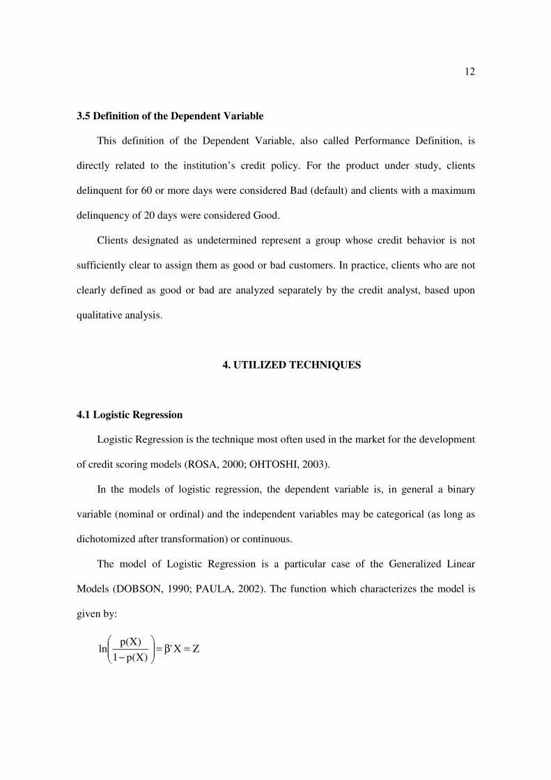
The model of Logistic Regression is a particular case of the Generalized Linear

Models (DOBSON, 1990; PAULA, 2002). The function which characterizes the model is

given by:

ZX')X(p1

)X(pln =β=��

�

����

�

−

13

),...,,,(' n210 ββββ=β : vector of the parameters associated to the variables

p(X)=E(Y=1|X): probability of the individual has been classified as good, given the

vector X.

This probability is expressed by (NETER et al., 1996: 580):

Z

Z

X'

X'

e1

e

e1

e)Y(E)X(p

+=

+==

β

β

Initially, in this work all variables will be included for the construction of the model;

however in the final logistic model, only some of the variables will be selected. The choice

of the variables will be done by means of the method forward stepwise, which is the most

widely used in models of logistic regression. For the details on the methodology reading of

Canton (1988: 28) and Neter et al. (1996: 348), is suggested.

Fensterstock (2005: 48) points out the following advantages in using logistic

regression for the construction of models:

• The generated model takes into account the correlation between variables,

identifying relationships that would not be visible and eliminating redundant

variables;

• It takes into account the variables individually and simultaneously;

• The user may check the sources of error and optimize the model.

In the same text, the author further identifies some disadvantages of this technique:

• In many cases preparation of the variables takes a long time;

14

• In the case of many variables the analyst must perform a pre-selection of the more

important, based upon separate analyses:

• Some of the resulting models are difficult to implement.

4.2 Artificial Neural Networks

Artificial Neural Networks are computational techniques that present a mathematical

model based upon the neural structure of intelligent organisms and who acquire knowledge

through experience.

It was only in the eighties that, because of the greater computational power, neural

networks were widely studied and applied. Fausett (1994: 25) underlines the development

of the backpropagation algorithm as the turning point for the popularity of neural networks.

An artificial neural network model processes certain characteristics and produces

replies like those of the human brain. Artificial neural networks are developed using

mathematical models in which the following suppositions are made (FAUSETT, 1994: 3):

1. Processing of information takes place within the so-called neurons;

2. Stimuli are transmitted by the neurons through connections;

3. Each connection is associated to a weight which, in a standard neural network,

multiplies itself upon receiving a stimulus;

4. Each neuron contributes for the activation function (in general not linear) to

determine the output stimulus (response of the network).

The pioneer model by McCulloch and Pitts from 1943 for one processing unit (neuron)

can be summarized in:

15

• Signals are presented upon input;

• Each signal is multiplied by a weight that indicates its influence on the output of

the unit;

• The weighted sum of the signals which produces a level of activity is made;

• If this level exceeds a limit, the unit produces an output.

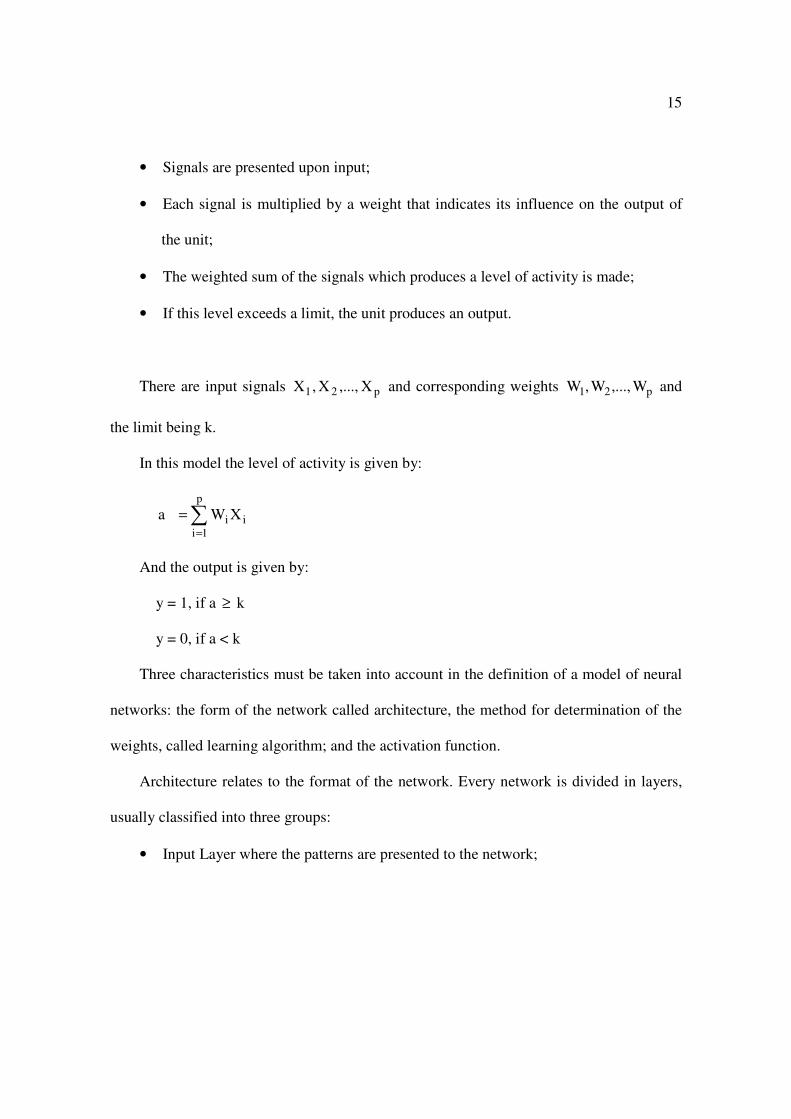
There are input signals p21 X,...,X,X and corresponding weights p21 W,...,W,W and

the limit being k.

In this model the level of activity is given by:

�=

=p

1iii XWa

And the output is given by:

y = 1, if a ≥ k

y = 0, if a < k

Three characteristics must be taken into account in the definition of a model of neural

networks: the form of the network called architecture, the method for determination of the

weights, called learning algorithm; and the activation function.

Architecture relates to the format of the network. Every network is divided in layers,

usually classified into three groups:

• Input Layer where the patterns are presented to the network;

16

• Intermediate or Hidden layers in which the major part of processing takes place, by

means of the weighted connections, they may be viewed as extractors of

characteristics;

• Output Layer, in which the end result is concluded and presented.

There are basically three main types of architecture (HAYKIN, 1999: 46-48):

feedforward networks with a single layer; feedforward networks with multiple layers and

recurring networks.

1. Feedforward networks with a single layer are the simpler network, in which there

is only one input layer and one output layer. Some networks utilizing this

architecture are: the Hebb Network, perceptron, ADALINE, among others.

2. Multilayered feedforward networks are those having one or more intermediate

layers. The multilayer perceptron networks (MLP), MADALINE and of a radial

base function are some of the networks utilizing this architecture.

3. Recurrent networks: in this type of network, the output layer has at least one

connection that feeds back the network. The networks called BAM (Biderectional

Associative Memory) and ART1 and ART2 (Adaptative Resonance Theory) are

recurring networks.

The most important quality of neural networks is the capacity to “learn” according to

the environment and thereby improve their performance (CASTRO JR., 2003: 92).

There are essentially three types of learning:

17

1. Supervised Learning: in this type of learning the expected reply is indicated to the

network. This is the case of this work, where a priori it is already known whether

the client is good or bad.

2. Non-supervised Learning: in this type of learning the network must only rely on

the received stimuli; the network must learn to cluster the stimuli;

3. Reinforcement Learning: in this type of learning, behavior of the network is

assessed by an external reviewer.

Berry and Linoff (1997: 331) point out the following positive points in the utilization

of neural networks:

• They are versatile: neural networks may be used for the solution of different types

of problems such as: prediction, clustering or identification of patterns;

• They are able to identify non-linear relationships between variables;

• They are widely utilized, can be found in various software.

As for the disadvantages the authors state:

• Results cannot be explained: no explicit rules are produced, analysis is performed

inside the network and only the result is supplied by the “black box”;

• The network can converge towards a lesser solution: there are no warranties that

the network will find the best possible solution; it may converge to a local

maximum.

4.3 Genetic Algorithms

18

The idea of genetic algorithms resembles the evolution of the species proposed by

Darwin: the algorithms will evolve with the passing of generations and the candidates for

the solution of the problem one wants to solve “stay alive” and reproduce (BACK et al.,

1996).

The algorithm is comprised of a population which is represented by chromosomes that

are merely the various possible solutions for the proposed problem. Solutions that are

selected to shape new solutions (starting from a cross-over) are selected according to the

fitness of the parent chromosomes. Thus, the more fit the chromosome is, the higher the

possibility of reproducing itself. This process is repeated until the rule of halt is satisfied,

that is to say to find a solution very near to that hoped for.

Every genetic algorithm goes through the following stages:

Start: initially a population is generated formed by a random set of individuals

(chromosomes) that may be viewed as possible solutions for the problem.

Fitness: a function of fitness is defined to evaluate the “quality” of each one of the

chromosomes.

Selection: according to the results of the fitness function, a percentage of the best fit is

maintained while the others are rejected (Darwinism).

Cross-over: two parents are chosen and based upon them an offspring is generated,

based on a specific cross-over criterion. The same criterion is used with another

chromosome and the material of both chromosomes is exchanged. If there is no cross-over,

the offspring is an exact copy of the parents.

Mutation is an alteration in one of the genes of the chromosome. The purpose of

mutation is to avoid that the population converges to a local maximum. Thus, should this

19

convergence take place, mutation ensures that the population will jump over the minimum

local point, endeavoring to reach other maximum points.

Verification of the halt criterion: once a new generation is created, the criterion of halt

is verified and should this criterion not have been met, one returns to the stage of the fitness

function.

The following positive points in the utilization of genetic algorithms must be

highlighted:

• Contrariwise to neural networks they produce explicable results (BERRY;

LINOFF, 1997: 357);

• Their use is easy (BERRY; LINOFF, 1997: 357);

• They may work with a large set of data and variables (FENSTERSTOCK, 2005:

48).

Some of the disadvantages pointed out in literature are:

• They continue to be seldom used for problems of assessment of risk credit

(FENSTERSTOCK, 2005: 48);

• Require a major computational effort (BERRY; LINOFF, 1997: 358);

• Are available in only a few softwares (BERRY; LINOFF, 1997: 358).

4.4 Criteria for Performance Evaluation

To evaluate performance of the model two samples were selected, one for validation

and the other for test. Both were of the same size (3,000 clients considered good and 3,000

20

considered bad, for each one). In addition to the samples, other criteria are used, which are

presented in this section.

Score of Hits

The score of hits is measured by dividing the total of clients correctly classified, by the

number of clients included in the model.

Similarly, the score of hits of the good and bad clients can be quantified.

In some situations it is much more important to identify a good client than a bad client

(or vice versa); in such cases, often a more fitting weight is given to the score of hits and a

weighted mean of the score of hits is calculated.

In this work, as there is not a priori information on what would be more attractive for

the financial institution (identification of the good or bad clients), the product between the

score of hits of good and bad clients (Ih) will be used as an indicator of hits to evaluate the

quality of the model. This indicator will privilege the models with high scores of hits for

both types of clients. The greater the indicator is the better will be the model.

The Kolmogorov-Smirnov Test

The Kolmogorov-Smirnov (KS) is the other criterion often used in practice and used in

this work (PICININI et al., 2003; OOGHE et al., 2001; Pereira, 2004).

The KS test is a non-parametric technique to determine whether two samples were

collected from the same population (or from populations with similar distributions)

(SIEGEL, 1975: 144). This test is based on the accumulated distribution of the scores of

clients considered good and bad.

21

To check whether the samples have the same distribution, there are tables to be

consulted according to the significance level and size of the sample (see SIEGEL, 1975:

309-310). In this work, as the samples are large, tendency is that all models reject the

hypothesis of equal distributions. The best model will be that with the highest value in the

test, because this result indicates a larger spread between the good and bad.

5. APPLICATION

This section will cover the methods to treat variables, the application of the three

techniques under study and the results obtained by each one of them, comparing their

performance. For descriptive analysis, categorization of data and application of logistic

regression the SPSS for Windows v.11.0 software was used, the software Enterprise Miner.

4.1 was used for the selection of the samples and application to the neural network; for the

genetic algorithm a program developed in Visual Basic by the authors was utilized.

5.1 Treatment of the Variables

Initially, the quantitative variables were categorized.

The deciles (values below which 10%, 20% etc. of the cases fall) of these variables

were initially identified for categorization of the continuous variables. Starting from the

deciles, the next step was to analyze them according to the dependent variable. The

distribution of good and bad clients was calculated by deciles and then the ratio between

good and bad was calculated, the so called relative risk (RR).

Groups presenting a similar relative risk (RR) were re-grouped to reduce the number

of categories by variable.

22

The relative risks were also calculated for the qualitative variables to reduce the

number of categories, whenever possible. According to Pereira (2004: 49) there are two

reasons to make a new categorization of the qualitative variables. The first is to avoid

categories with a very small number of observations, which may lead to less robust

estimates of the parameters associated to them. The second is the elimination of the model

parameters, if two categories present a close risk, it is reasonable to group them in one

single class.

Besides clustering of categories, RR helps to understand whether this category is more

connected to good or to bad clients. This method of clustering categories is explained by

Hand and Henley (1997: 527).

When working with the variables made available, heed was given to the following:

• The variables gender, first acquisition and type of credit were not re-coded as they

are already binary variables;

• The variable profession was clustered according to the similarity of the nature of

jobs;

• The variables commercial telephone and home telephone were recoded in the

binary form as ownership or not;

• The variables commercial ZIP Code and home ZIP Code were initially clustered

according to the first three digits, next the relative risk of each layer was calculated

and later a reclustering was made according to the similar relative risk, the same

procedure adopted by Rosa (2000: 17) as explained by Hand and Henley (1997:

527);

23

• The variable salary of the spouse was discarded from the analysis because much

data was missing;

• Two new variables were created, percentage of the amount loaned on the salary

and percentage of the amount of the installment on the salary. Both are quantitative

variables, which where categorized in the same way as the remainder.

After applying this method, the categories shown on Table 1 were obtained.

Insert Table 1 about here

5.2 Logistic Regression

For the estimation of the model of logistic regression, a sample of 8,000 cases equally

divided in the categories of good or bad was utilized.

Initially, it is interesting to evaluate the logistic relationship between each independent

variable and the dependent variable TYPE.

Since one of the objectives of this analysis was to identify which variables are more

efficient for the characterization of the two types of bank clients, a stepwise procedure was

utilized. The elected method of selection was forward stepwise.

Of the 53 available independent variables, considering k-1 dummies for each variable

of k levels, 28 variables were included in the model.

In this study, Z is the linear combination of the 28 independent variables weighted by

the logistic coefficients:

24

Z = B0 + B1.X1 + B2.X2 + ........+ B28.X28

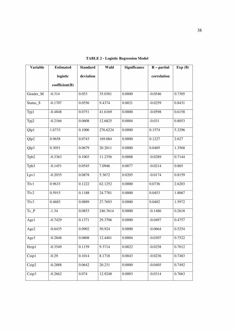
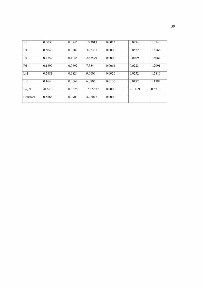
Table 2 shows, per variable, the estimates of the logistic coefficients, the standard

deviations of the estimates, the Wald statistics and the descriptive levels of the significance

tests of independent variables.

Insert Table 2 about here

With categorical variables, evaluation of the effect of one particular category must be

done in comparison with a reference category. The coefficient for the reference category is

0.

Variables with a logistic coefficient estimated negative indicate that the focused

category, with regard to the reference, is associated to a decrease of the odds and therefore

a decrease in the probability of having a good client.

The coefficient of partial correlation is a measurement of the power of relation

between the dependent variable and an independent variable, keeping constant the effects

of the other independent variables. Variables that most affect positively the probability of

having a good client are Qlp1, Qlp2 and Tlv1. At the opposite end the variables with a

greater negative impact on this probability are Tc_P, Fa_N and Age2.

Table 2 shows that the coefficients of all variables included in the logistic model are

statistically different from zero. Therefore, all have shown to be relevant for the

discrimination between good and bad clients.

25

There are two statistical tests to evaluate the significance of the final model: the chi-

square test of the change in the value of – 2LL (-2 times the log of the likelihood) and the

Hosmer and Lemeshow test.

Table 3 presents the initial value of – 2LL, considering only the model’s constant, its

end value, the improvement and the descriptive level to measure its significance.

Insert Table 3 about here

The model of 28 variables disclosed that the reduction of the -2LL measure was

statistically significant.

The Hosmer and Lemeshow test considers the statistical hypothesis that the predicted

classifications in groups are equal to those observed. Therefore, this is a test of the fitness

of the model to the data.

The chi-square statistic presented the outcome 3.4307, with eight degrees of freedom

and descriptive level equal to 0.9045. This outcome leads to the non rejection of the null

hypothesis of the test, endorsing the model’s adherence to the data.

5.3 Neural Network

In this work, a supervised learning network will be used, as it is known a priori

whether the clients in question are good or bad. According to Potts (1998: 44), the most

used structure of neural network for this type of problem is the multilayer perceptron

26

(MLP) which is a network with a feedforward architecture with multiple layers. Consulted

literature (ARMINGER et al., 1997; ARRAES et al., 1999; ZERBINI, 2000; CASTRO JR.,

2003; OHTOSHI, 2003) supports this statement. The network MLP will also be adopted in

this work.

The MLP networks can be trained using the following algorithms: Conjugate

Descending Gradient, Levenberg-Marquardt, Back propagation, Quick propagation or

Delta-bar-Delta. The more common (CASTRO JR., 2003: 142) is the Back propagation

algorithm which will be detailed later on. For the understanding of the others, reading of

Fausett (1994) and Haykin (1999) is suggested.

The implemented model has an input layer of neurons, a single neuron output layer,

which corresponds to the outcome whether a client is good or bad in the classification of

the network. It also has an intermediate layer with three neurons, since it was the network

which presented the best outcomes, in the query of the higher percentage of hits as well as

in the query of reduction of the mean error. Networks which had one, two or four neurons

were also tested in this work.

Each neuron of the hidden layer is a processing element that receives n inputs

weighted by weights Wi. The weighted sum of inputs is transformed by means of a

nonlinear activation function f(.).

The activation function used in this study will be the logistic function, )g(e1

1−+

,

where

�=

=p

1iii XWg is the weighted sum of the neuron inputs.

27

Training of the networks consists in finding the set of Wi weights that minimizes one

function of error. In this work for the training will be used the Back propagation algorithm.

In this algorithm the network operates in a two step sequence. First a pattern is presented to

the input layer of the network. The resulting activity flows through the network, layer by

layer until the reply is produced by the output layer. In the second step the output achieved

is compared to the desired output for this particular pattern. If not correct, the error is

estimated. The error is propagated starting from the output layer to the input layer, and the

weights of the connections of the units of the inner layers are being modified, while the

error is backpropagated. This procedure is repeated in the successive iterations until the halt

criterion is reached.

In this model the halt criterion adopted was the mean error of the set of validation data.

This error is calculated by means of the module of the difference between the value the

network has located and the expected one. Its mean for the 8,000 cases (training sample) or

the 6,000 cases (validation sample) is estimated. Processing detected that the stability of the

model took place after the 94th iteration. In the validation sample the error was somewhat

larger (0.62 x 0.58), which is common considering that the model is fitted based upon the

first sample.

Initially, the bad classification is of 50%, because the allocation of an individual as a

good or bad client is random; with the increase of the iterations, the better result of 30.6%

of error is reached for the training sample and of 32.3% for the validation sample.

Some of the statistics of the adopted network are in Table 4.

28

Insert Table 4 about here

Besides the misclassification and the mean error, the square error and the degrees of

freedom are also presented. The average square error is calculated by the average of the

squares of the differences between that observed and that obtained from the network.

The number of degrees of freedom of the model is related to the number of estimated

weights, to the connection of each of the attributes to the neurons of the intermediate layer

and to the binding of the intermediate layer with the output.

5.4 Genetic Algorithms

The genetic algorithm was used to find a discriminate equation permitting to score

clients, and later, separate the good from the bad according to the score achieved. The

equation scores the clients and those with a higher score are considered good, while the bad

are those with a lower score. This route was adopted by Kishore et al. (2000) and Picinini et

al. (2003).

The implemented algorithm was similar to that presented in Picinini et al. (2003). Each

one of the 71 categories of variables was given an initial random weight. To these seventy

one coefficients, one more was introduced, an additive constant incorporated to the linear

equation. The value of the client score is given by:

( )�=

=72

1iijij pwS , where

jS = Score obtained by client j

29

iw = Weight relating to the category i

ijp = binary indicator equal to 1, if the client j has the category i and 0, conversely.

The following rule was used to define if the client is good or bad:

If 0S j ≥ , the client is considered good

If 0S j < , the client is considered bad

As such, the problem the algorithm has to solve is to find the vector W=

[ 7221 w,...,w,w ] resulting in a classification criterion with a good rate of hits in predicting

the performance of payment of credit.

Following the stages of a genetic algorithm, one has:

Start: a population of 200 individuals was generated with each chromosome holding

72 genes. The initial weight iw of each gene was randomly generated in the interval [-1, 1]

(PICININI et al., 2003: 464).

Fitness Function: each client was associated to the estimate of a score and classified as

good or bad. By comparing with the information already known a priori on the nature of the

client, the precision of each chromosome can be calculated. The indicator of hits (Ih), will

be the fitness function, that is to say, the greater the indicator the better will be the

chromosome.

Selection: In this work an elitism of 10% was used, that is to say, for each new

generation, the twenty best chromosomes are maintained while the other hundred and

eighty are formed by cross over and mutation.

Cross-over: to chose the parents for cross-over the method known as roulette wheel

was used for selection among these twenty chromosomes that were maintained (CHEN;

30

HUANG, 2003: 436-437). In this method, each individual is given one probability of being

drawn according to its value of the fitness function.

For the process of exchange of genetic material a method known as uniform cross-over

was used (PAPPA, 2002: 22). In this type of cross-over each gene of the offspring

chromosome is randomly chosen among the genes of one of the parents, while the second

offspring receives the complementary genes of the second father.

Mutation: in the mutation process, each gene of the chromosome is independently

evaluated. Each gene of each chromosome has a 0.5% probability of undergoing mutation.

Whenever a gene is chosen for mutation, the genetic alteration is performed, adding a small

scalar value k in this gene. In the described experiment a value ranging from -0.05 and +

0.05 was randomly drawn.

Verification of the halt criterion: a maximum number of generations equal to 600 was

defined as the halt criterion. After six hundred iterations, the fit chromosome will be the

solution.

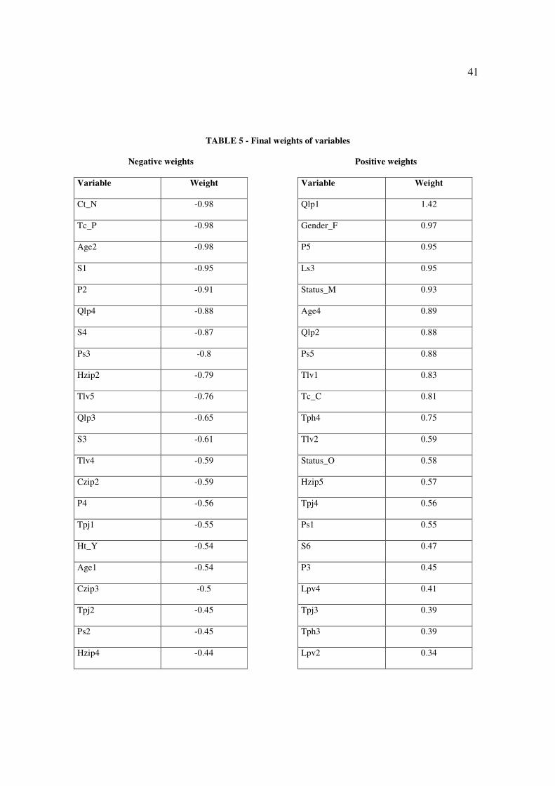
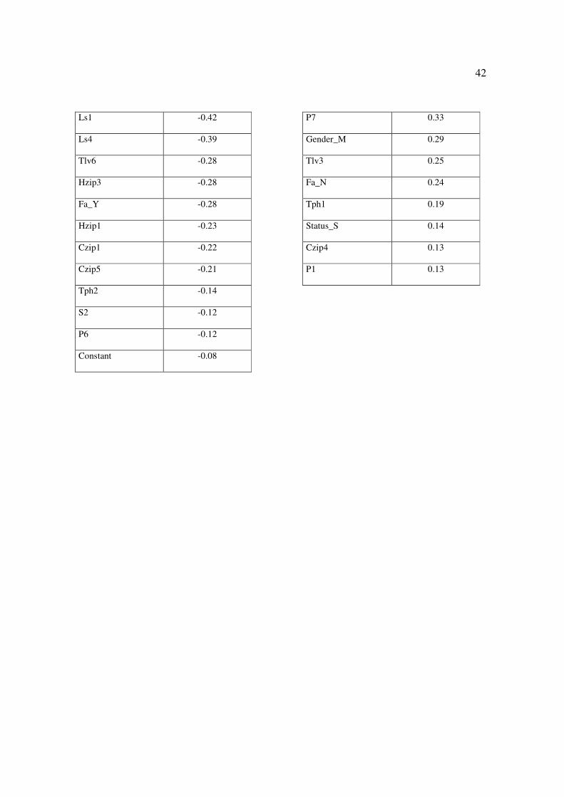
Results of the algorithm that had the highest Indicator of hits are presented here.

After execution of the algorithm, variables with a very small weight were discarded. In

the work by Picinini et al. (2003: 464) the authors consider that the variables with a weight

lower than 0.15 or higher than -0.15 would be discarded because they did not have a

significant weight for the model. In this work, after performing a sensitivity analysis, it was

decided that the variables with a weight higher than 0.10 or lower than – 0.10 would be

considered significant for the model. This rule was not applied for the constant, which was

proven important for the model even with a value below cutoff. Weight of the variables is

shown in Table 5.

31

Insert Table 5 about here

Negative weight indicates that the variable has a greater relationship with the clients

considered bad (since it was determined that clients with a total negative score would be

viewed as bad). The positive weight, conversely, is related with good clients.

Comparing these results with those achieved by logistic regression, an agreement

between the variables with a higher weight is perceived. In both models, the variable with

higher negative weight was the variable Tc_P and with the higher positive weight was Qlp1

(in both models this was the variable with the highest absolute weight). Other variables

such as Tpj1, Age2, Qlp2, Tlv1, Tlv2 are also among the higher weight variables in both

models, substantiating that the result of the algorithm was coherent.

5.5 Evaluation of the Models’ Performance

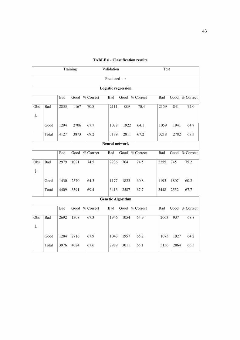
After obtaining the models the three samples were scored and the Ih and KS were

calculated for each of the models. Table 6 shows the results of classification reached by the

three models.

Insert Table 6 about here

32

All presented good classification results, because, according to Picinini et al. (2003:

465): “credit scoring models with hit rates above 65% are considered good by specialists”.

The hit percentages were very similar in the models of logistic regression and neural

network and were somewhat lesser for the model of genetic algorithms. Another interesting

result is that, except for genetic algorithms, the models presented the greatest rate of hits for

bad clients, with a higher than 70% rate for bad clients in the three samples of the logistic

and neural network models.

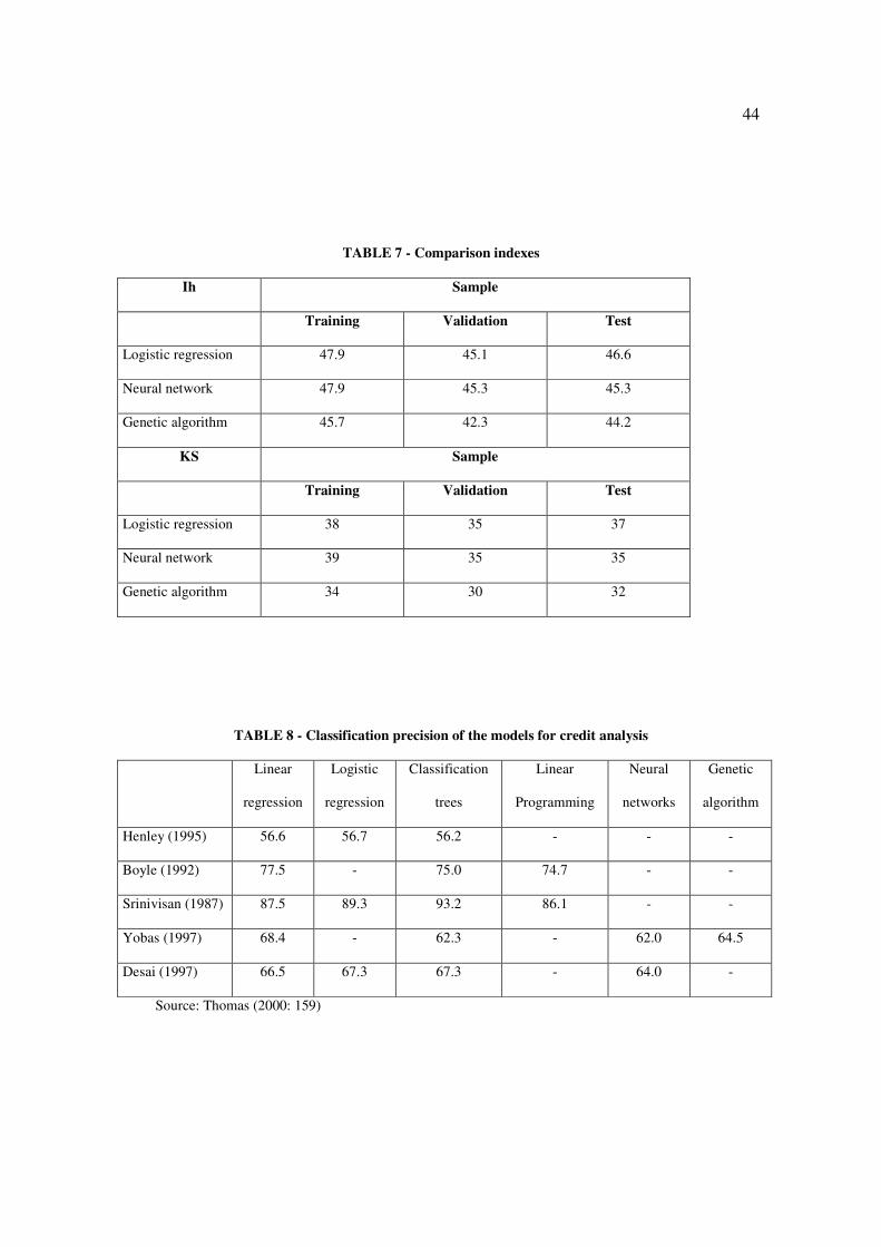
Table 7 presents results of the criteria Ih and KS which were chosen to compare the

models.

Insert Table 7 about here

KS values in all models can be considered good. Again, Picinini et al. (2003: 465)

explain: “The Kolmogorov-Smirov test (KS) is used in the financial market as one of the

efficiency indicators of the credit scoring models. A model which presents a KS value

equal or higher than 30 is considered good by the market”. Here again, the logistic

regression and neural network models exhibit very close results, superior to those achieved

by the genetic algorithm.

In choosing the model that best fits these data and analyzing according to the Ih and

KS indicators, the model built by logistic regression was elected. Although results were

very similar to those achieved by neural networks this model presented the best results in

the test sample, suggesting that it is best fit for application in other databases. Nevertheless,

33

it must be highlighted that the adoption of any one of the models would bring about good

results for the financial institution.

6. CONCLUSIONS AND RECOMMENDATIONS

The objective of this study was to develop credit scoring predictive models based upon

data of a large financial institution by using Logistic Regression, Artificial Neural

Networks and Genetic Algorithms.

When developing the credit scoring models some care must be taken to guarantee the

quality of the model and its later applicability. Precautions in the sampling, clear definition

of criteria for the classification of good and bad clients and treatment of variables in the

database prior to application of the techniques were the measures taken in this study,

aiming to optimize results and minimize errors.

The three models presented suitable results for the database in question, which was

supplied by a large retail bank operating in Brazil. The logistic regression model presented

slightly better results to the model built by neural networks and both were better than the

model based on genetic algorithms. The model proposed by this study to enable the

institution to score its clients is:

Z

Z

e1

e)X(p

+=

p: probability of the client being considered good and

Z = B0 + B1.X1 + B2.X2 + ........+ B28.X28 , where the values of Bi and Xi are found in

Table 2.

34

For the test sample the percentage of total hits for logistic regression, neural networks

and genetic algorithms was respectively equal to 68.3; 67.7 and 66.5. In the literature

consulted, the percentage of total hits fluctuates significantly, as well as the model that best

fits each data bank can be different from that obtained in this study. Table 8, taken from the

work by Thomas (2000), shows the range of results achieved in other works.

Insert Table 8 about here

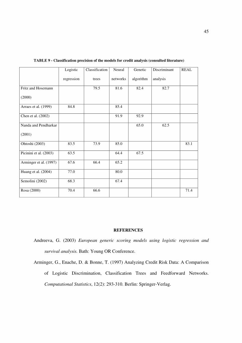
Table 9, built from the surveyed literature, is similar to the previous table and

strengthens the wide variety of results.

Insert Table 9 about here

When these two tables are analyzed it should be noted that the models present a

precision of classification ranging from 56.2 to 93.2. Further it is noted that except for the

linear programming, all the other models presented the greatest precision, in at least one of

the studies.

This study did not aim at a more detailed approach of the techniques focused. Neural

networks and genetic algorithms presented an extensive range of structures and variations

that may (and must) be better explored. Genetic algorithms, as they are a rather flexible

method, not yet widely researched in problems of credit concession, may be used in diverse

forms to optimize results.

35

In this type of problem, new techniques such as survival analysis should not be

overlooked and merit attention in future studies.

36

TABLE 1 - Categorized Variables

Variable Category Variable name

Gender Masculine Feminine Gender_M Gender_F

Marital status Married Single other Status_M Status_S Status_O

Home telephone Yes No Ht_Y Ht_N

Commercial telephone Yes No Ct_Y Ct_N

Time in the present job Until 24 months, 25 to 72, 73 to 127, More

than 127

Tpj1 Tpj2 Tpj3 Tpj4

Salary Up to US 283, 284 to 413, 414 to 685, 686 to

876, 877 to 1304, More than 1304

S1 S2 S3 S4 S5 S6

Quantity of loan parts Up to 4, 5 to 6, 7 to 9, 10 to 12 Qlp1 Qlp2 Qlp3 Qlp4

First acquisition Yes No Fa_Y Fa_N

Time in the present home Until 12 months, 13 to 24, 25 to 120, More

than 120

Tph1 Tph2 Tph3 Tph4

Loan part value Up to US 54, 55 to 70, 71 to 113, More than

113

Lpv1 Lpv2 Lpv3 Lpv4

Total loan value Up to US 131, 132 to 174, 175 to 217, 218 to

348, 349 to 783, More than 783

Tlv1 Tlv2 Tlv3 Tlv4 Tlv5

Tlv6

Type of credit Passbook check Tc_P Tc_C

Age Until 25 years, 26 to 40, 41 to 58, More than

58

Age1 Age2 Age3 Age4

Range of home ZIP Code 1 2 3 4 5 Hzip1 Hzip2 Hzip3 Hzip4

Hzip5

Range commercial ZIP

Code

1 2 3 4 5 Czip1 Czip2 Czip3 Czip4

Czip5

37

Profession code 1 2 3 4 5 6 7 P1 P2 P3 P4 P5 P6 P7

Percent rate of part /

salary

Up to 10%, 10.1% to 13.5%, 13.6% to 16.5%,

16.6% to 22.5%, More than 22.5%

Ps1 Ps2 Ps3 Ps4 Ps5

Percent rate of loan /

salary

Up to 28%, 28.1% to 47.5%, 47.6% to 65%,

More than 65%

Ls1 Ls2 Ls3 Ls4 Ls5

Type of client 1 = good 0 = bad Type

38

TABLE 2 - Logistic Regression Model

Variable Estimated

logistic

coefficient(B)

Standard

deviation

Wald Significance R – partial

correlation

Exp (B)

Gender_M -0.314 0.053 35.0381 0.0000 -0.0546 0.7305

Status_S -0.1707 0.0556 9.4374 0.0021 -0.0259 0.8431

Tpj1 -0.4848 0.0751 41.6169 0.0000 -0.0598 0.6158

Tpj2 -0.2166 0.0608 12.6825 0.0004 -0.031 0.8053

Qlp1 1.6733 0.1006 276.6224 0.0000 0.1574 5.3296

Qlp2 0.9658 0.0743 169.084 0.0000 0.1227 2.627

Qlp3 0.3051 0.0679 20.2011 0.0000 0.0405 1.3568

Tph2 -0.3363 0.1003 11.2356 0.0008 -0.0289 0.7144

Tph3 -0.1451 0.0545 7.0946 0.0077 -0.0214 0.865

Lpv1 -0.2035 0.0878 5.3672 0.0205 -0.0174 0.8159

Tlv1 0.9633 0.1222 62.1252 0.0000 0.0736 2.6203

Tlv2 0.5915 0.1188 24.7781 0.0000 0.0453 1.8067

Tlv3 0.4683 0.0889 27.7693 0.0000 0.0482 1.5972

Tc_P -1.34 0.0853 246.7614 0.0000 -0.1486 0.2618

Age1 -0.7429 0.1371 29.3706 0.0000 -0.0497 0.4757

Age2 -0.6435 0.0902 50.924 0.0000 -0.0664 0.5254

Age3 -0.2848 0.0808 12.4401 0.0004 -0.0307 0.7522

Hzip1 -0.3549 0.1159 9.3714 0.0022 -0.0258 0.7012

Czip1 -0.29 0.1014 8.1718 0.0043 -0.0236 0.7483

Czip2 -0.2888 0.0642 20.231 0.0000 -0.0405 0.7492

Czip3 -0.2662 0.074 12.9248 0.0003 -0.0314 0.7663

39

P1 0.3033 0.0945 10.3013 0.0013 0.0274 1.3543

P3 0.5048 0.0889 32.2381 0.0000 0.0522 1.6566

P5 0.4752 0.1048 20.5579 0.0000 0.0409 1.6084

P6 0.1899 0.0692 7.534 0.0061 0.0223 1.2091

Ls1 0.2481 0.0824 9.0609 0.0026 0.0252 1.2816

Ls3 0.164 0.0664 6.0906 0.0136 0.0192 1.1782

Fa_N -0.6513 0.0526 153.5677 0.0000 -0.1169 0.5213

Constant 0.5868 0.0903 42.2047 0.0000

40

TABLE 3 - Chi-Square test

-2LL Chi-Square

(improvement)

Degrees of

freedom

Significance

11090.355

9264.686 1825.669 28 0.000

TABLE 4 - Neural network statistics

Obtained statistics Test Validation

Misclassification of cases 0.306 0.323

Mean error 0.576 0.619

Mean square error 0.197 0.211

Degrees of freedom of the model 220

Degrees of freedom of the error 7780

Total degrees of freedom 8000

41

TABLE 5 - Final weights of variables

Negative weights Positive weights

Variable Weight Variable Weight

Ct_N -0.98 Qlp1 1.42

Tc_P -0.98 Gender_F 0.97

Age2 -0.98 P5 0.95

S1 -0.95 Ls3 0.95

P2 -0.91 Status_M 0.93

Qlp4 -0.88 Age4 0.89

S4 -0.87 Qlp2 0.88

Ps3 -0.8 Ps5 0.88

Hzip2 -0.79 Tlv1 0.83

Tlv5 -0.76 Tc_C 0.81

Qlp3 -0.65 Tph4 0.75

S3 -0.61 Tlv2 0.59

Tlv4 -0.59 Status_O 0.58

Czip2 -0.59 Hzip5 0.57

P4 -0.56 Tpj4 0.56

Tpj1 -0.55 Ps1 0.55

Ht_Y -0.54 S6 0.47

Age1 -0.54 P3 0.45

Czip3 -0.5 Lpv4 0.41

Tpj2 -0.45 Tpj3 0.39

Ps2 -0.45 Tph3 0.39

Hzip4 -0.44 Lpv2 0.34

42

Ls1 -0.42 P7 0.33

Ls4 -0.39 Gender_M 0.29

Tlv6 -0.28 Tlv3 0.25

Hzip3 -0.28 Fa_N 0.24

Fa_Y -0.28 Tph1 0.19

Hzip1 -0.23 Status_S 0.14

Czip1 -0.22 Czip4 0.13

Czip5 -0.21 P1 0.13

Tph2 -0.14

S2 -0.12

P6 -0.12

Constant -0.08

43

TABLE 6 - Classification results

Training Validation Test

Predicted →

Logistic regression

Bad Good % Correct Bad Good % Correct Bad Good % Correct

Obs

↓

Bad 2833 1167 70.8 2111 889 70.4 2159 841 72.0

Good 1294 2706 67.7 1078 1922 64.1 1059 1941 64.7

Total 4127 3873 69.2 3189 2811 67.2 3218 2782 68.3

Neural network

Bad Good % Correct Bad Good % Correct Bad Good % Correct

Obs

↓

Bad 2979 1021 74.5 2236 764 74.5 2255 745 75.2

Good 1430 2570 64.3 1177 1823 60.8 1193 1807 60.2

Total 4409 3591 69.4 3413 2587 67.7 3448 2552 67.7

Genetic Algorithm

Bad Good % Correct Bad Good % Correct Bad Good % Correct

Obs

↓

Bad 2692 1308 67.3 1946 1054 64.9 2063 937 68.8

Good 1284 2716 67.9 1043 1957 65.2 1073 1927 64.2

Total 3976 4024 67.6 2989 3011 65.1 3136 2864 66.5

44

TABLE 7 - Comparison indexes

Ih Sample

Training Validation Test

Logistic regression 47.9 45.1 46.6

Neural network 47.9 45.3 45.3

Genetic algorithm 45.7 42.3 44.2

KS Sample

Training Validation Test

Logistic regression 38 35 37

Neural network 39 35 35

Genetic algorithm 34 30 32

TABLE 8 - Classification precision of the models for credit analysis

Linear

regression

Logistic

regression

Classification

trees

Linear

Programming

Neural

networks

Genetic

algorithm

Henley (1995) 56.6 56.7 56.2 - - -

Boyle (1992) 77.5 - 75.0 74.7 - -

Srinivisan (1987) 87.5 89.3 93.2 86.1 - -

Yobas (1997) 68.4 - 62.3 - 62.0 64.5

Desai (1997) 66.5 67.3 67.3 - 64.0 -

Source: Thomas (2000: 159)

45

TABLE 9 - Classification precision of the models for credit analysis (consulted literature)

Logistic

regression

Classification

trees

Neural

networks

Genetic

algorithm

Discriminant

analysis

REAL

Fritz and Hosemann

(2000)

79.5 81.6 82.4 82.7

Arraes et al. (1999) 84.8 85.4

Chen et al. (2002) 91.9 92.9

Nanda and Pendharkar

(2001)

65.0 62.5

Ohtoshi (2003) 83.5 73.9 85.0 83.1

Picinini et al. (2003) 63.5 64.4 67.5

Arminger et al. (1997) 67.6 66.4 65.2

Huang et al. (2004) 77.0 80.0

Semolini (2002) 68.3 67.4

Rosa (2000) 70.4 66.6 71.4

REFERENCES

Andreeva, G. (2003) European generic scoring models using logistic regression and

survival analysis. Bath: Young OR Conference.

Arminger, G., Enache, D. & Bonne, T. (1997) Analyzing Credit Risk Data: A Comparison

of Logistic Discrimination, Classification Trees and Feedforward Networks.

Computational Statistics, 12(2): 293-310. Berlin: Springer-Verlag.

46

Arraes, D., Semolini, R. & Picinini, R. (1999) Arquiteturas de Redes Neurais Aplicadas a

Data Mining no Mercado Financeiro. Uma Aplicação para a Geração de Credit

Ratings. In: IV Brazilian Congress of Neural Nets.

Back, B., Laitinen, T. & Sere, K. (1996) Neural Networks and Genetic Algorithms for

Bankruptcy Predictions. In: Proceedings of the 3rd World Conference on Expert

Systems: 123-130.

Berry, M. & Linoff, G. (1997) Data Mining Techniques. New York: Wiley.

Canton, A. W. P. (1988) Aplicação de modelos estatísticos na avaliação de produtos

(Dept. of Business Administration University of São Paulo, Brazil).

Caouette, J., Altmano, E. & Narayanan, P. (2000) Gestão do Risco de Crédito. Rio de

Janeiro: Qualitymark.

Castro Jr., F. H. F. (2003) Previsão de Insolvência de Empresas Brasileiras Usando

Análise Discriminante, Regressão Logística e Redes Neurais. (Dept. of Business

Administration University of São Paulo, Brazil).

Chen, M.-C. & Huang, S.-H. (2003) Credit scoring and rejected instances reassigning

through evolutionary computation techniques. Expert Systems with Applications,

24(4): 433-441. St. Louis: Elsevier Science.

Chen, M.-C., Huang, S.-H. & Chen, C.-M. (2002) Credit Classification Analysis through

the Genetic Programming Approach. Taipei: Proceedings of the 2002 International

Conference in Information Management. Tamkang University.

Dobson, A. (1990) An Introduction to Generalized Linear Models. London: Chapman &

Hall.

Fausett, L. (1994) Fundamentals of Neural Networks. Englewood-Cliffs: Prentice-Hall.

47

Fensterstock, F. (2005) Credit Scoring and the Next Step. Business Credit, 107(3): 46-49.

New York: National Association of Credit Management.

Figueiredo, R. P. (2001) Gestão de Riscos Operacionais em Instituições Financeiras –

Uma Abordagem Qualitativa. (Dept. of Business Administration University of

Amazônia, Brazil).

Fritz, S. & Hosemann, D. (2000) Restructuring the Credit Process: Behaviour Scoring for

German Corporates. International Journal of Intelligent Systems in Accounting,

Finance and Management, 9(1): 9-21. Nottingham: John Wiley & Sons.

Hand, D. J. & Henley, W. E. (1997) Statistical Classification Methods in Consumer Credit

Scoring: a Review. Journal of Royal Statistical Society: Series A (160): 523-541.

London: Royal Statistical Society.

Harrison, T. & Ansell, J. (2002) Customer retention in the insurance industry: using

survival analysis to predict cross-selling opportunities. Journal of Financial Services

Marketing, 6(3): 229-239. London: Henry Stewart Publications.

Haykin, S. (1999) Redes Neurais Princípios e Prática. Porto Alegre: Bookman.

Huang, Z., Chen, H., HSU, C-J., Chen, W. & Wu, S. (2004) Credit rating analysis with

support vector machines and neural networks: a market comparative study. Decision

Support Systems, 37(4): 543-558. St. Louis: Elsevier Science.

Kishore, J. K., Patnaik, L. M., Mani, V. & Agrawal, V. K. (2000) Application of genetic

programming for multicategory pattern classification. IEEE Transactions on

Evolutionary Computation, 4(3): 242-257. Birmingham: IEEE Computational

Intelligence Society.

Lewis, E. M. (1992) An Introduction to Credit Scoring. San Rafael: Fair Isaac and Co., Inc.

48

Nanda, S. & Pendharkar, P. (2001) Linear models for minimizing misclassification costs in

bankruptcy prediction. International Journal of Intelligent Systems in Accounting,

Finance and Management, 10(3): 155-168. Nottingham: John Wiley & Sons.

Neter, J., Kutner, M. H., Nachtshein, C. J. & Wasserman, W. (1996) Applied Linear

Statistical Models. Chicago: Irwin.

Ohtoshi, C. (2003) Uma Comparação de Regressão Logística, Árvores de Classificação e

Redes Neurais: Analisando Dados de Crédito. (Dept. of Statistics, University of São

Paulo, Brazil).

Ooghe, H., Camerlynck, J. & Balcaen, S. (2001) The Ooghe-Joos-De Vos Failure

Prediction Models: A Cross-Industry Validation. (Department of Corporate Finance.

University of Ghent.)

Pappa, G. L. (2002) Seleção de Atributos Utilizando Algoritmos Genéticos Multiobjetivos.

Dissertação de Mestrado. (Dept. of Informatics, Pontifical Catholic University of

Paraná, Brazil).

Paula, G. A. (2002) Modelos de Regressão com Apoio Computacional. Book available in

http://www.ime.usp.br/~giapaula/livro.pdf accessed in 12/05/2004.

Pereira, G. H. A. (2004) Modelos de risco de crédito de clientes: Uma aplicação a dados

reais. Dissertação de Mestrado. Departamento de Estatística. Universidade de São

Paulo. IME/USP.

Picinini, R., Oliveira, G. M. B. & Monteiro, L. H. A. (2003) Mineração de Critério de

Credit Scoring Utilizando Algoritmos Genéticos. in: VI Brazilian Symposium of

Intelligent Automation 463-466.

49

Potts, W. J. E. (1998) Data Mining Primer Overview of Applications and Methods. Carrie:

SAS Institute Inc.

Rosa, P. T. M. (2000) Modelos de Credit Scoring: Regressão Logística, CHAID e REAL.

(Dept. of Statistics, University of São Paulo, Brazil).

Santos, J. O. (2000) Análise de Crédito: Empresas e Pessoas Físicas. São Paulo: Atlas.

Semolini, R. (2002) Support Vector Machines, Inferência Transdutiva e o Problema de

Classificação. (Dept. of Electric Engineer University of Campinas, Brazil).

Siegel, S. (1975) Estatística Não-Paramétrica para as Ciências do Comportamento. São

Paulo: McGraw-Hill.

Thomas, L. (2000) A Survey of Credit and Behavioural Scoring: Forecasting Financial

Risk of Lending to Consumers. International Journal of Forecasting, 16(2): 149-172.

London: Elsevier.

Trevisani, A. T., Gonçalves, E. B., D’Emídio, M. & Humes, L. L. (2004) Qualidade de

Dados – Desafio Crítico para o Sucesso do Business Intelligence. In: XVIII Latin

American Congress of Strategy.

Zerbini, M. B. A. A. (2000) Três Ensaios sobre Crédito. (Dept. of Economy, University of

São Paulo, Brazil).