INTRODUCTIONSPREADSHEET HINTS AND TIPS

This introduction covers procedures that you’ll use in the exercises throughoutthis book. It is intended to be a ready reference, and as such it has a different for-mat than the exercises. The first two exercises, “Mathematical Functions andGraphs” and “Spreadsheet Functions and Macros,” apply some of the proceduresdiscussed here to the exercise format and give you an opportunity to practice them.

If you are already familiar with spreadsheets, you may want to skip this chap-ter, or perhaps just check out any unfamiliar topics. To help you find what you’reinterested in, here’s an outline:

Starting Up: p. 2Menus and Commands: p. 2Spreadsheet Structure: p. 4Selecting (Highlighting) Cells: p. 4Copying Cell Contents: p. 5Cutting Cell Contents: p. 5Pasting Into a Cell: p. 5Cell Addresses: p. 5Entering Literals: p. 5Entering Formulae: p. 7Calculation Operators in Formulae: p. 7Entering Functions: p. 9Array Functions: p. 10Relative and Absolute Cell Addresses: p. 12Filling a Series: p. 12Formatting Cells: p. 13Creating a Graph: p. 14Editing a Graph: p. 16Automatic and Manual Calculation: p. 16Macros: p. 16Glossary of Terms and Symbols p. 18

Three warnings: First, this chapter is not a substitute for your spreadsheet user’smanual. We base our instructions throughout the book on Microsoft Excel, andmost will work as written in other spreadsheets, but there may be differences inthe details. If you follow our instructions carefully, and they don’t work, con-

sult your spreadsheet user’s manual. Second, you should already be familiar with somebasic computer skills, such as booting up your computer, starting your spreadsheetprogram, saving files, and printing. If you’re not, consult your operating system user’smanual. Third, save your work frequently to disk! Few things are as frustrating asspending hours building a model, then losing all your hard work when the computercrashes.

Starting UpHow you start up your spreadsheet program will depend on whether you use a Mac-intosh, an IBM-compatible computer, or a UNIX computer, whether the computer ison a network or not, and which spreadsheet program you choose. Consult your oper-ating system manual, your spreadsheet program manual, or a local computer expert.

All of the exercises in this book were developed with Microsoft Excel version 98 orhigher, which utilizes the “Visual Basic for Applications” code. If you are using an olderversion of Excel or a different spreadsheet program, make sure the basic functions usedin the exercise are available. Some exercises require the use of the Solver function, anoptimization function that is within the spreadsheet’s Add-In Pak. Your system admin-istrator may need to help you install the Solver

These exercises were written by several authors, using either Macintosh or Windowsplatforms; most, however, were developed in Windows. Table 1 gives some alternativecommands and keystrokes that may help if the instructions are not tailored to yourmachine.

Menus and CommandsMost spreadsheet programs have graphical user interfaces in which you use a mouseto choose commands from menus across the top of the screen. Many menus have sub-

2 Introduction

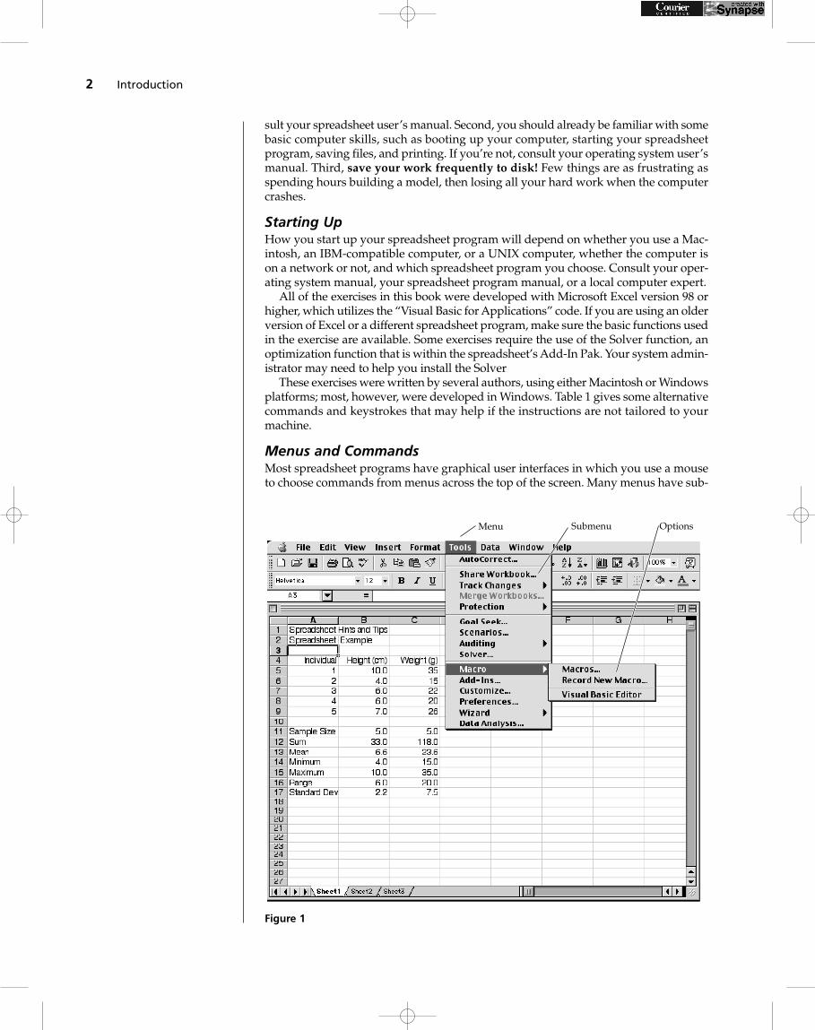
Figure 1

Menu Submenu Options

menus, and/or options as shown in Figure 1. Your mouse may have one, two, or threebuttons. All operations described in this section are performed with the left button. Incurrent Macintosh and Windows operating systems, a single mouse-click will open amenu and keep it open. To execute a command from a menu, move the cursor over theavailable commands until the one you want is highlighted, and then click the mousea second time. On Macintoshes running older operating systems, you must click the

Spreadsheet Hints and Tips 3

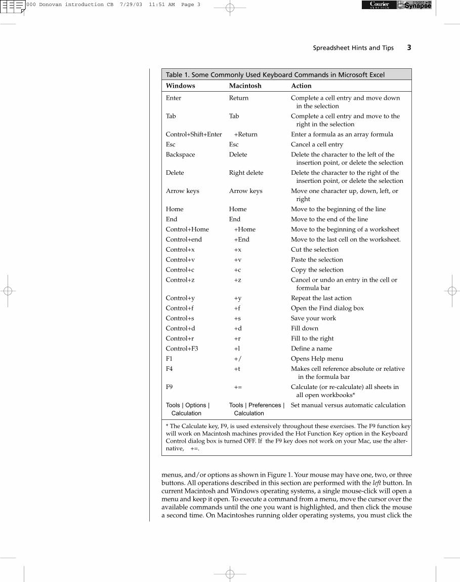
Table 1. Some Commonly Used Keyboard Commands in Microsoft Excel

Windows Macintosh Action

Enter Return Complete a cell entry and move down in the selection

Tab Tab Complete a cell entry and move to the right in the selection

Control+Shift+Enter +Return Enter a formula as an array formula

Esc Esc Cancel a cell entry

Backspace Delete Delete the character to the left of the insertion point, or delete the selection

Delete Right delete Delete the character to the right of the insertion point, or delete the selection

Arrow keys Arrow keys Move one character up, down, left, or right

Home Home Move to the beginning of the line

End End Move to the end of the line

Control+Home +Home Move to the beginning of a worksheet

Control+end +End Move to the last cell on the worksheet.

Control+x +x Cut the selection

Control+v +v Paste the selection

Control+c +c Copy the selection

Control+z +z Cancel or undo an entry in the cell or formula bar

Control+y +y Repeat the last action

Control+f +f Open the Find dialog box

Control+s +s Save your work

Control+d +d Fill down

Control+r +r Fill to the right

Control+F3 +l Define a name

F1 +/ Opens Help menu

F4 +t Makes cell reference absolute or relativein the formula bar

F9 += Calculate (or re-calculate) all sheets in all open workbooks*

Tools | Options | Tools | Preferences | Set manual versus automatic calculationCalculation Calculation

* The Calculate key, F9, is used extensively throughout these exercises. The F9 function keywill work on Macintosh machines provided the Hot Function Key option in the KeyboardControl dialog box is turned OFF. If the F9 key does not work on your Mac, use the alter-native, +=.

000 Donovan introduction CB 7/29/03 11:51 AM Page 3

mouse button and hold it down as you move the cursor down the menu options. Releasethe mouse button when the command you want is highlighted. The command will flashwhen it is successfully invoked.

For instance, if you wanted to record a macro in your spreadsheet to carry out a setof instructions, you would open the Tools menu, select the Macro submenu, and choosethe Record New Macro Option. Throughout this book we will use the vertical bar (|)and sans serif type (Menu) to indicate a menu, submenu, or option. Thus, the instructionabove would read, “Open Tools | Macro | Record New Macro.” The results of this opera-tion are shown in Figure 1 (and discussed in more detail on p. 16).

Many menu commands also have keyboard shortcuts—key combinations that youcan press to execute the command without having to open a menu and sort through itssubmenus and options. Shortcuts are listed next to the commands in the menus, andalways begin with <Control> in Windows and with on a Macintosh, followed usu-ally by a single letter (see Table 1). To use a shortcut, press and hold the <Control> orthe key while simultaneously typing the indicated letter. We will represent this simul-taneous key-pressing like this: +c on (Macs) or <Control>+c (Windows). This is theshortcut for Edit | Copy. Many people use shortcuts for frequently used commands, andyou may find it worthwhile to memorize a few of these, such as the one for copy, and+v (Macs), <Control>+v (Windows) for Edit | Paste.

Don’t be afraid to thrash around in the menus. In other words, if you’re not sure howto do something, try opening menus and submenus, searching for a command that lookslike it might work. Try different commands and see what happens. This is how welearned most of what we know about spreadsheets. However, be sure to save your workbefore you start to thrash—then, just in case you do something that messes up your work,you can close the file without saving any of the changes you made and the file will revertto what it was before you started thrashing.

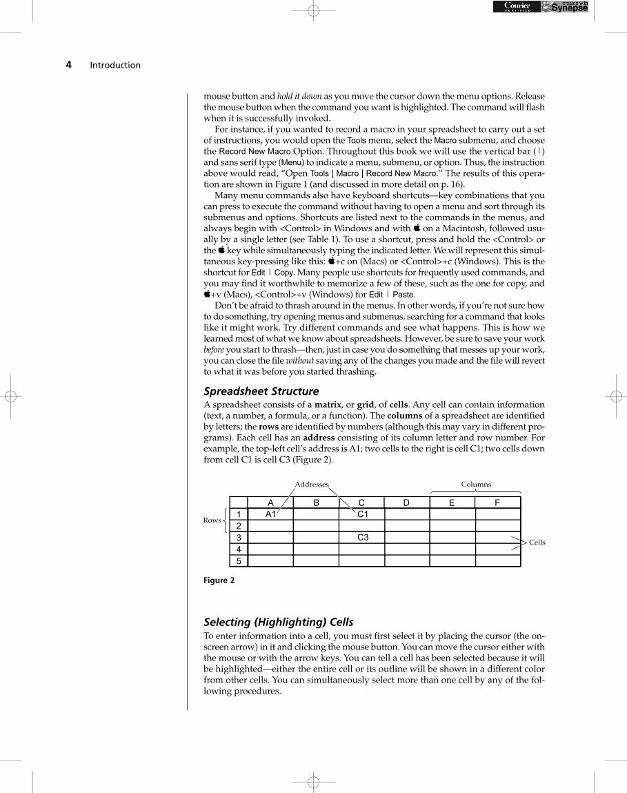
Spreadsheet StructureA spreadsheet consists of a matrix, or grid, of cells. Any cell can contain information(text, a number, a formula, or a function). The columns of a spreadsheet are identifiedby letters; the rows are identified by numbers (although this may vary in different pro-grams). Each cell has an address consisting of its column letter and row number. Forexample, the top-left cell’s address is A1; two cells to the right is cell C1; two cells downfrom cell C1 is cell C3 (Figure 2).

Selecting (Highlighting) CellsTo enter information into a cell, you must first select it by placing the cursor (the on-screen arrow) in it and clicking the mouse button. You can move the cursor either withthe mouse or with the arrow keys. You can tell a cell has been selected because it willbe highlighted—either the entire cell or its outline will be shown in a different colorfrom other cells. You can simultaneously select more than one cell by any of the fol-lowing procedures.

4 Introduction

12345

A B C D E F

Cells

A1 C1

C3

Rows

Addresses Columns

Figure 2

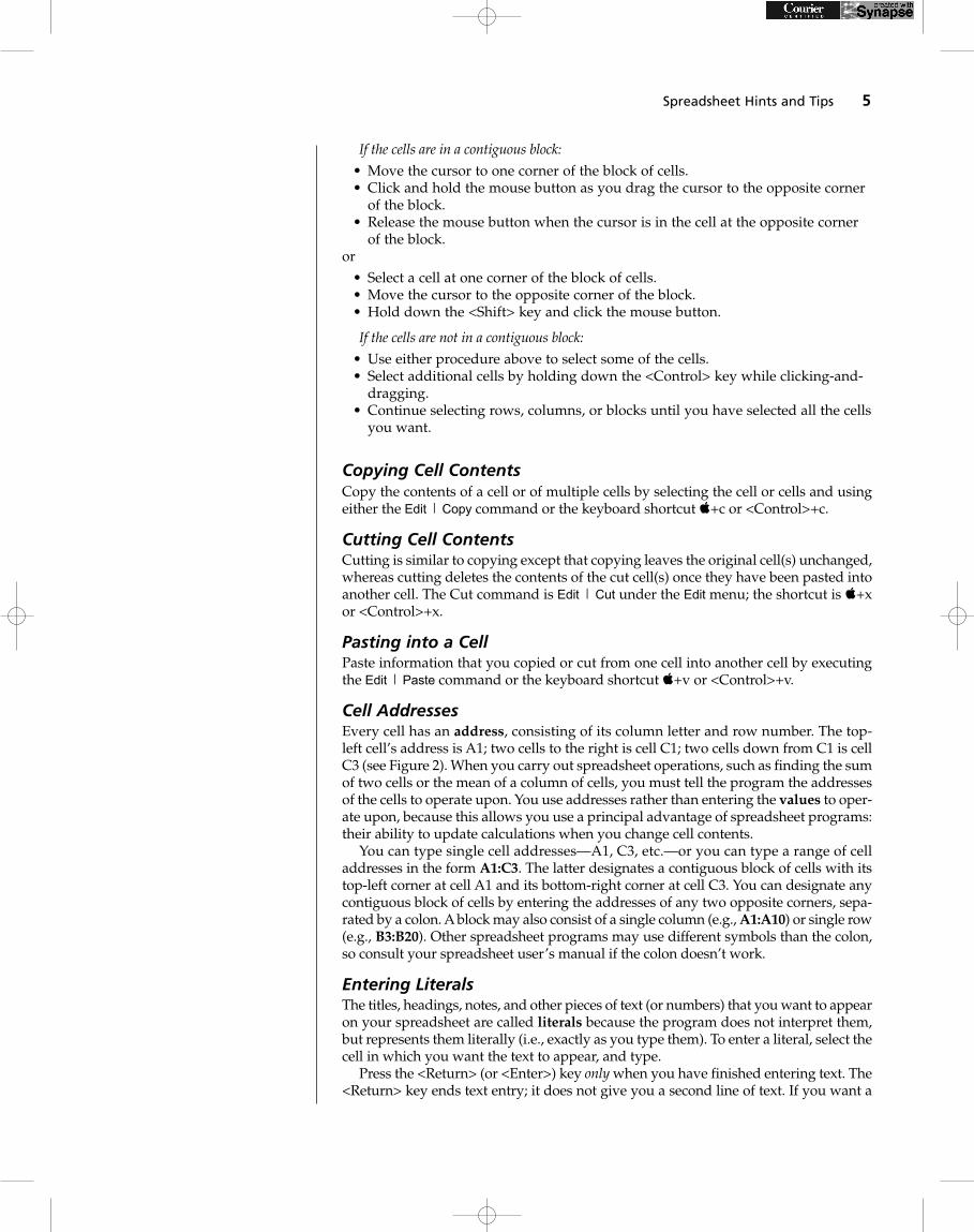
If the cells are in a contiguous block:

• Move the cursor to one corner of the block of cells.• Click and hold the mouse button as you drag the cursor to the opposite corner

of the block.• Release the mouse button when the cursor is in the cell at the opposite corner

of the block.or

• Select a cell at one corner of the block of cells.• Move the cursor to the opposite corner of the block.• Hold down the <Shift> key and click the mouse button.

If the cells are not in a contiguous block:

• Use either procedure above to select some of the cells.• Select additional cells by holding down the <Control> key while clicking-and-

dragging.• Continue selecting rows, columns, or blocks until you have selected all the cells

you want.

Copying Cell ContentsCopy the contents of a cell or of multiple cells by selecting the cell or cells and usingeither the Edit | Copy command or the keyboard shortcut +c or <Control>+c.

Cutting Cell ContentsCutting is similar to copying except that copying leaves the original cell(s) unchanged,whereas cutting deletes the contents of the cut cell(s) once they have been pasted intoanother cell. The Cut command is Edit | Cut under the Edit menu; the shortcut is +xor <Control>+x.

Pasting into a CellPaste information that you copied or cut from one cell into another cell by executingthe Edit | Paste command or the keyboard shortcut +v or <Control>+v.

Cell AddressesEvery cell has an address, consisting of its column letter and row number. The top-left cell’s address is A1; two cells to the right is cell C1; two cells down from C1 is cellC3 (see Figure 2). When you carry out spreadsheet operations, such as finding the sumof two cells or the mean of a column of cells, you must tell the program the addressesof the cells to operate upon. You use addresses rather than entering the values to oper-ate upon, because this allows you use a principal advantage of spreadsheet programs:their ability to update calculations when you change cell contents.

You can type single cell addresses—A1, C3, etc.—or you can type a range of celladdresses in the form A1:C3. The latter designates a contiguous block of cells with itstop-left corner at cell A1 and its bottom-right corner at cell C3. You can designate anycontiguous block of cells by entering the addresses of any two opposite corners, sepa-rated by a colon. A block may also consist of a single column (e.g., A1:A10) or single row(e.g., B3:B20). Other spreadsheet programs may use different symbols than the colon,so consult your spreadsheet user’s manual if the colon doesn’t work.

Entering LiteralsThe titles, headings, notes, and other pieces of text (or numbers) that you want to appearon your spreadsheet are called literals because the program does not interpret them,but represents them literally (i.e., exactly as you type them). To enter a literal, select thecell in which you want the text to appear, and type.

Press the <Return> (or <Enter>) key only when you have finished entering text. The<Return> key ends text entry; it does not give you a second line of text. If you want a

Spreadsheet Hints and Tips 5

label of more than one line, one way is to type the first line, press <Return> or the downarrow key, place the cursor in the cell below (if it’s not already there), and type the sec-ond line. Another way is to type all the text into a single cell and then format the cell toturn on text wrapping (see p. 13 for how to format cells).

As you type text or numbers into a cell, what you type will appear in the cell and inthe formula bar above the spreadsheet column headings (Figure 3). If you make a mis-take, use your mouse to place the cursor on the mistake either in the cell or in the for-mula bar. Then use the backspace or delete key to erase the mistake, or highlight themistake using click-and-drag, and retype. The text will appear in the selected cell afteryou press <Return>. If you discover an error later, you can simply select the cell againand correct your mistake as above.

Sometimes strange things happen when you enter a literal, depending on your pro-gram and how it is set up. For instance, if you enter 5-10 (meaning a range of valuesfrom 5 to 10), the cell may show May 10. This is because the program interprets someentries as dates. To force the program to treat your entry as a literal, precede it with anapostrophe, ‘5-10, or open Format | Cells | General.

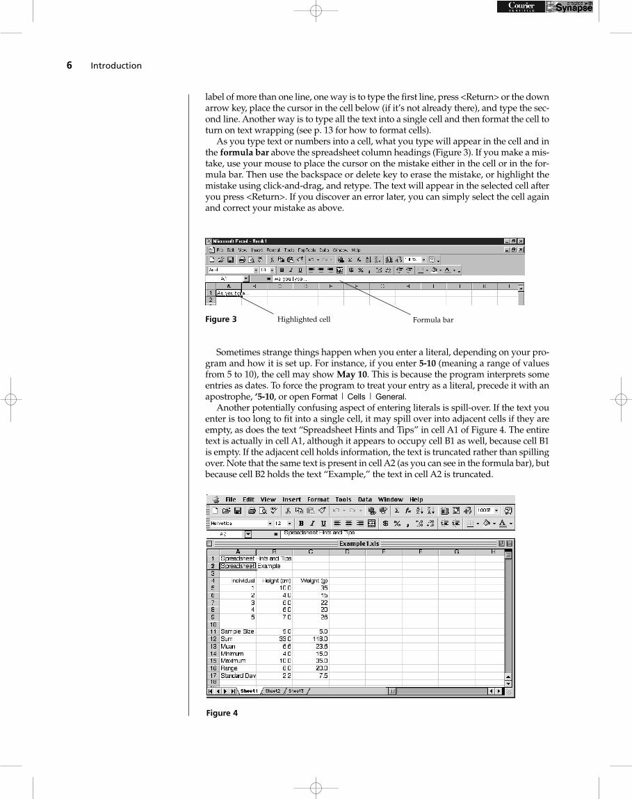
Another potentially confusing aspect of entering literals is spill-over. If the text youenter is too long to fit into a single cell, it may spill over into adjacent cells if they areempty, as does the text “Spreadsheet Hints and Tips” in cell A1 of Figure 4. The entiretext is actually in cell A1, although it appears to occupy cell B1 as well, because cell B1is empty. If the adjacent cell holds information, the text is truncated rather than spillingover. Note that the same text is present in cell A2 (as you can see in the formula bar), butbecause cell B2 holds the text “Example,” the text in cell A2 is truncated.

6 Introduction

Figure 3 Highlighted cell Formula bar

Figure 4

Entering FormulaeA very important part of spreadsheet programming is entering formulae. A formulatells the spreadsheet to carry out some operation(s) on the contents of one or more cells,and to place the result into the cell where the formula is. A formula usually containsone or more cell addresses and operations to be performed on the contents of the ref-erenced cells. A formula must begin with a symbol to alert the spreadsheet that it is aformula rather than a literal. In Excel, the symbol is typically the equal sign (=), butother symbols (such as +) may work in this or other spreadsheet programs.

Two useful tips to remember regarding formulas:• The formula appears in the formula bar as you type it, and it will appear there

again if you select the cell later. But once you press <Return>, only the result ofthe formula appears in the cell itself.

• A formula may not refer to the cell in which it resides; therefore, e.g., do notenter the formula =2*B2 into cell B2. This will generate an error message com-plaining about a “circular reference.”

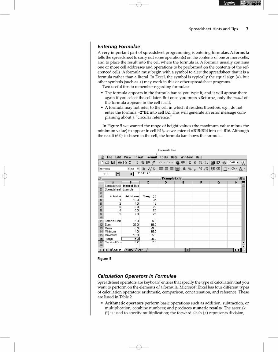
In Figure 5 we wanted the range of height values (the maximum value minus theminimum value) to appear in cell B16, so we entered =B15-B14 into cell B16. Althoughthe result (6.0) is shown in the cell, the formula bar shows the formula.

Calculation Operators in FormulaeSpreadsheet operators are keyboard entries that specify the type of calculation that youwant to perform on the elements of a formula. Microsoft Excel has four different typesof calculation operators: arithmetic, comparison, concatenation, and reference. Theseare listed in Table 2.

• Arithmetic operators perform basic operations such as addition, subtraction, ormultiplication; combine numbers; and produces numeric results. The asterisk(*) is used to specify multiplication; the forward slash (/) represents division;

Spreadsheet Hints and Tips 7

Figure 5

Formula bar

and the carat (^) represents exponentiation (raising to a power). Otherarithemetic operators include the standard + and -.

• Comparison operators compare two values (for example, whether two valuesare equal, or one is greater than the other) and return a logical value—eithertrue or false—for specified calculations.

• The ampersand (&) is the text concatenation operator. It joins, or “concate-nates” two strings of text to produce a continues text string.

• Reference operators are the colon (:) and the comma (,). These operators com-bine ranges of cells for calculations.

If you combine several operations in a single formula, Microsoft Excel performs theoperations in the order shown in Table 3. If a formula contains multiple operators withthe same precedence (i.e., if a formula contains both a multiplication and a division oper-ator), the program evaluates the operators from left to right. You can change the orderof evaluation by enclosing the part of the formula to be calculated first in parentheses.

8 Introduction

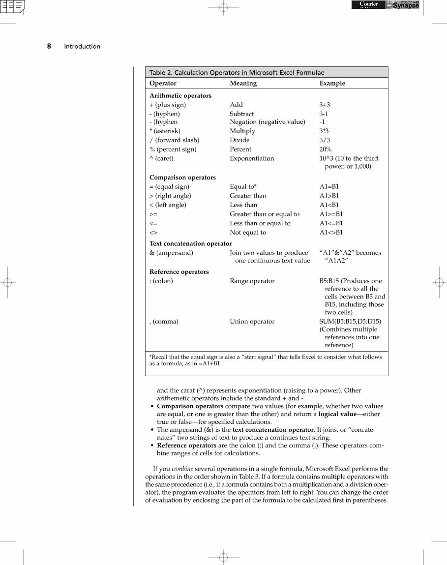
Table 2. Calculation Operators in Microsoft Excel Formulae

Operator Meaning Example

Arithmetic operators+ (plus sign) Add 3+3- (hyphen) Subtract 3-1- (hyphen Negation (negative value) -1* (asterisk) Multiply 3*3/ (forward slash) Divide 3/3% (percent sign) Percent 20%^ (caret) Exponentiation 10^3 (10 to the third

power, or 1,000)

Comparison operators= (equal sign) Equal to* A1=B1> (right angle) Greater than A1>B1< (left angle) Less than A1<B1>= Greater than or equal to A1>=B1<= Less than or equal to A1<=B1<> Not equal to A1<>B1

Text concatenation operator& (ampersand) Join two values to produce “A1”&”A2” becomes

one continuous text value “A1A2”

Reference operators: (colon) Range operator B5:B15 (Produces one

reference to all the cells between B5 andB15, including those two cells)

, (comma) Union operator SUM(B5:B15,D5:D15) (Combines multiple

references into one reference)

*Recall that the equal sign is also a “start signal” that tells Excel to consider what followsas a formula, as in =A1+B1.

Entering FunctionsA function is similar to a formula, but it usually carries out a more complex operationor set of operations, and it has been prewritten for you by the spreadsheet program-mers. We use functions extensively; many of the exercises in this book rely on them.Excel has over 100 functions, and you will probably not remember them all. Fortunately,most spreadsheet packages provide a simple means of entering functions so that youdon’t need to memorize them.

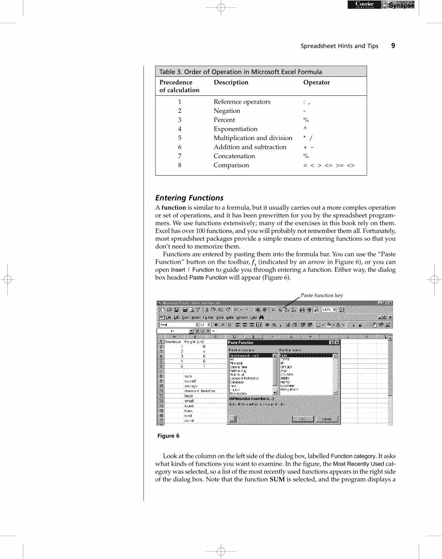
Functions are entered by pasting them into the formula bar. You can use the “PasteFunction” button on the toolbar, fx (indicated by an arrow in Figure 6), or you canopen Insert | Function to guide you through entering a function. Either way, the dialogbox headed Paste Function will appear (Figure 6).

Look at the column on the left side of the dialog box, labelled Function category. It askswhat kinds of functions you want to examine. In the figure, the Most Recently Used cat-egory was selected, so a list of the most recently used functions appears in the right sideof the dialog box. Note that the function SUM is selected, and the program displays a

Spreadsheet Hints and Tips 9

Table 3. Order of Operation in Microsoft Excel Formula

Precedence Description Operatorof calculation

1 Reference operators : ,2 Negation -3 Percent %4 Exponentiation ^5 Multiplication and division * /6 Addition and subtraction + –7 Concatenation %8 Comparison = < > <= >= <>

Figure 6

Paste function key

brief description of the SUM function at the bottom of the window. If you choose theFunction category All, you’ll see every function available, listed in alphabetical order.

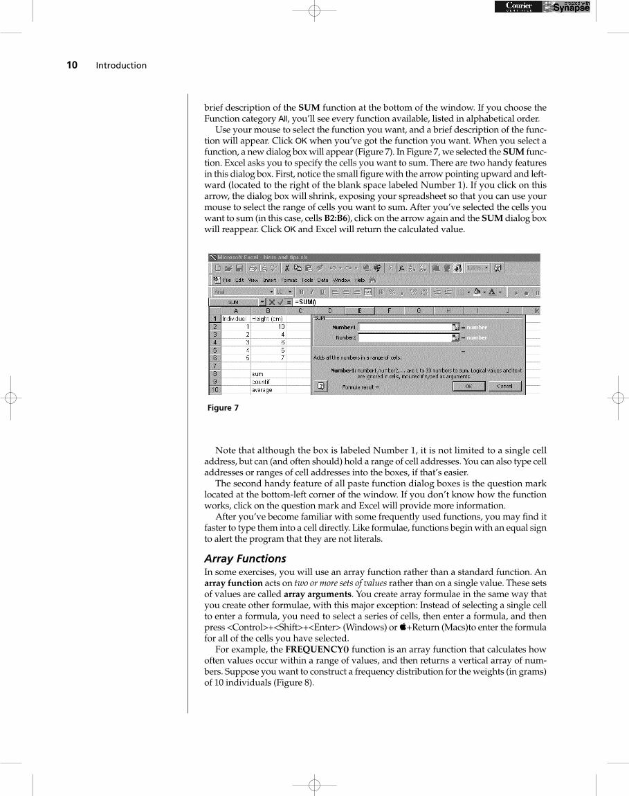
Use your mouse to select the function you want, and a brief description of the func-tion will appear. Click OK when you’ve got the function you want. When you select afunction, a new dialog box will appear (Figure 7). In Figure 7, we selected the SUM func-tion. Excel asks you to specify the cells you want to sum. There are two handy featuresin this dialog box. First, notice the small figure with the arrow pointing upward and left-ward (located to the right of the blank space labeled Number 1). If you click on thisarrow, the dialog box will shrink, exposing your spreadsheet so that you can use yourmouse to select the range of cells you want to sum. After you’ve selected the cells youwant to sum (in this case, cells B2:B6), click on the arrow again and the SUM dialog boxwill reappear. Click OK and Excel will return the calculated value.

Note that although the box is labeled Number 1, it is not limited to a single celladdress, but can (and often should) hold a range of cell addresses. You can also type celladdresses or ranges of cell addresses into the boxes, if that’s easier.

The second handy feature of all paste function dialog boxes is the question marklocated at the bottom-left corner of the window. If you don’t know how the functionworks, click on the question mark and Excel will provide more information.

After you’ve become familiar with some frequently used functions, you may find itfaster to type them into a cell directly. Like formulae, functions begin with an equal signto alert the program that they are not literals.

Array FunctionsIn some exercises, you will use an array function rather than a standard function. Anarray function acts on two or more sets of values rather than on a single value. These setsof values are called array arguments. You create array formulae in the same way thatyou create other formulae, with this major exception: Instead of selecting a single cellto enter a formula, you need to select a series of cells, then enter a formula, and thenpress <Control>+<Shift>+<Enter> (Windows) or +Return (Macs)to enter the formulafor all of the cells you have selected.

For example, the FREQUENCY() function is an array function that calculates howoften values occur within a range of values, and then returns a vertical array of num-bers. Suppose you want to construct a frequency distribution for the weights (in grams)of 10 individuals (Figure 8).

10 Introduction

Figure 7

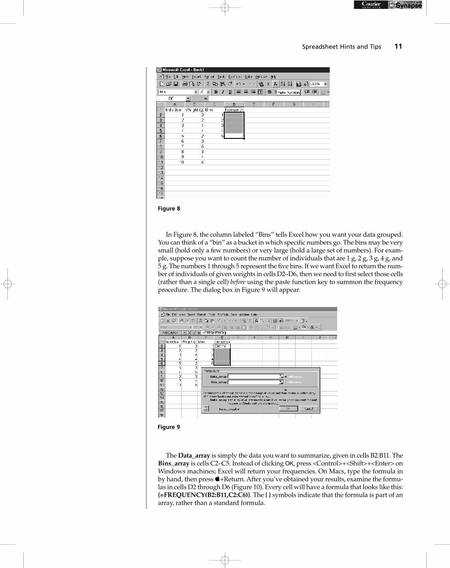
In Figure 8, the column labeled “Bins” tells Excel how you want your data grouped.You can think of a “bin” as a bucket in which specific numbers go. The bins may be verysmall (hold only a few numbers) or very large (hold a large set of numbers). For exam-ple, suppose you want to count the number of individuals that are 1 g, 2 g, 3 g, 4 g, and5 g. The numbers 1 through 5 represent the five bins. If we want Excel to return the num-ber of individuals of given weights in cells D2–D6, then we need to first select those cells(rather than a single cell) before using the paste function key to summon the frequencyprocedure. The dialog box in Figure 9 will appear.

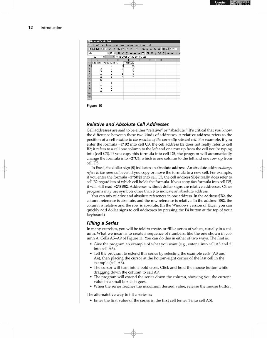
The Data_array is simply the data you want to summarize, given in cells B2:B11. TheBins_array is cells C2–C5. Instead of clicking OK, press <Control>+<Shift>+<Enter> onWindows machines; Excel will return your frequencies. On Macs, type the formula inby hand, then press +Return. After you’ve obtained your results, examine the formu-las in cells D2 through D6 (Figure 10). Every cell will have a formula that looks like this:{=FREQUENCY(B2:B11,C2:C6)}. The { } symbols indicate that the formula is part of anarray, rather than a standard formula.

Spreadsheet Hints and Tips 11

Figure 8

Figure 9

Relative and Absolute Cell AddressesCell addresses are said to be either “relative” or “absolute.” It’s critical that you knowthe difference between these two kinds of addresses. A relative address refers to theposition of a cell relative to the position of the currently selected cell. For example, if youenter the formula =2*B2 into cell C3, the cell address B2 does not really refer to cellB2; it refers to a cell one column to the left and one row up from the cell you’re typinginto (cell C3). If you copy this formula into cell D5, the program will automaticallychange the formula into =2*C4, which is one column to the left and one row up fromcell D5.

In Excel, the dollar sign ($) indicates an absolute address. An absolute address alwaysrefers to the same cell, even if you copy or move the formula to a new cell. For example,if you enter the formula =2*$B$2 into cell C3, the cell address $B$2 really does refer tocell B2 regardless of which cell holds the formula. If you copy this formula into cell D5,it will still read =2*$B$2. Addresses without dollar signs are relative addresses. Otherprograms may use symbols other than $ to indicate an absolute address.

You can mix relative and absolute references in one address. In the address $B2, thecolumn reference is absolute, and the row reference is relative. In the address B$2, thecolumn is relative and the row is absolute. (In the Windows version of Excel, you canquickly add dollar signs to cell addresses by pressing the F4 button at the top of yourkeyboard.)

Filling a SeriesIn many exercises, you will be told to create, or fill, a series of values, usually in a col-umn. What we mean is to create a sequence of numbers, like the one shown in col-umn A, Cells A5–A9 of Figure 11. You can do this in either of two ways. The first is:

• Give the program an example of what you want (e.g., enter 1 into cell A5 and 2into cell A6).

• Tell the program to extend this series by selecting the example cells (A3 andA4), then placing the cursor at the bottom-right corner of the last cell in theexample (cell A6).

• The cursor will turn into a bold cross. Click and hold the mouse button whiledragging down the column to cell A9.

• The program will extend the series down the column, showing you the currentvalue in a small box as it goes.

• When the series reaches the maximum desired value, release the mouse button.

The alternatetive way to fill a series is:• Enter the first value of the series in the first cell (enter 1 into cell A5).

12 Introduction

Figure 10

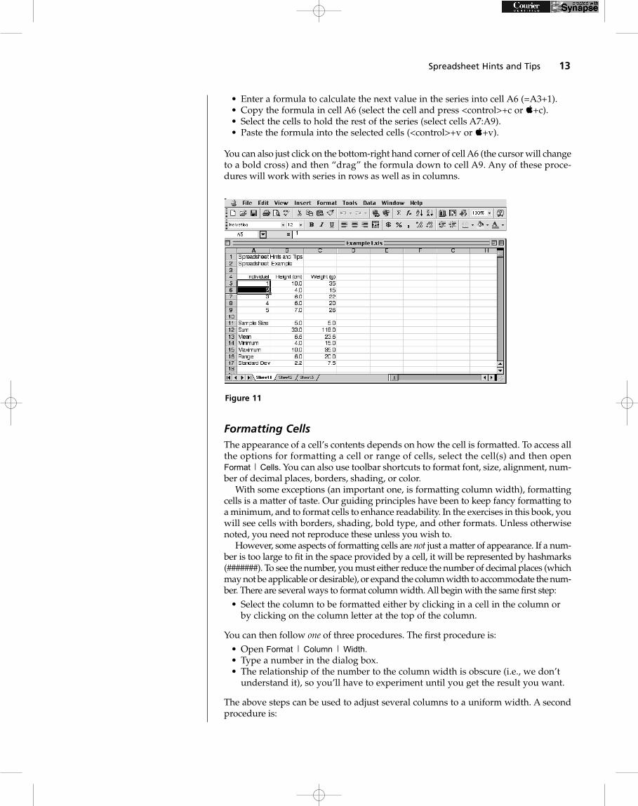
• Enter a formula to calculate the next value in the series into cell A6 (=A3+1).• Copy the formula in cell A6 (select the cell and press <control>+c or +c).• Select the cells to hold the rest of the series (select cells A7:A9).• Paste the formula into the selected cells (<control>+v or +v).

You can also just click on the bottom-right hand corner of cell A6 (the cursor will changeto a bold cross) and then “drag” the formula down to cell A9. Any of these proce-dures will work with series in rows as well as in columns.

Formatting CellsThe appearance of a cell’s contents depends on how the cell is formatted. To access allthe options for formatting a cell or range of cells, select the cell(s) and then open Format | Cells. You can also use toolbar shortcuts to format font, size, alignment, num-ber of decimal places, borders, shading, or color.

With some exceptions (an important one, is formatting column width), formattingcells is a matter of taste. Our guiding principles have been to keep fancy formatting toa minimum, and to format cells to enhance readability. In the exercises in this book, youwill see cells with borders, shading, bold type, and other formats. Unless otherwisenoted, you need not reproduce these unless you wish to.

However, some aspects of formatting cells are not just a matter of appearance. If a num-ber is too large to fit in the space provided by a cell, it will be represented by hashmarks(#######). To see the number, you must either reduce the number of decimal places (whichmay not be applicable or desirable), or expand the column width to accommodate the num-ber. There are several ways to format column width. All begin with the same first step:

• Select the column to be formatted either by clicking in a cell in the column orby clicking on the column letter at the top of the column.

You can then follow one of three procedures. The first procedure is:• Open Format | Column | Width.• Type a number in the dialog box.• The relationship of the number to the column width is obscure (i.e., we don’t

understand it), so you’ll have to experiment until you get the result you want.

The above steps can be used to adjust several columns to a uniform width. A secondprocedure is:

Spreadsheet Hints and Tips 13

Figure 11

• Open Format | Column | AutoFit Selection. Excel will adjust the column width topermit display of the widest element in the selected block or column.

A third alternative:• Place the cursor at the right-hand edge of the space around the letter at the top

of the column to be adjusted. The cursor will change to a vertical bar witharrows pointing to the right and the left.

• Click and hold down the mouse button.• While holding down the mouse button, drag to the right to widen the column

or to the left to narrow it.• When the column width is appropriate, release the mouse button.

Creating a GraphMost spreadsheet programs call graphs “charts.” We will follow scientific usage andcall them graphs. In these exercises, you’ll make lots of graphs. To create a graph (chart),you must tell the program:

• Which data to graph• To start a graph• Which kind of graph to use• Other details of how to set up the graph

Select data to graph by selecting the appropriate cells (see p. 4–5). Excel will alwaysplace the leftmost column or topmost row of data on the horizontal axis of the graph.If you want to change this, move columns or rows using the cut-and-paste proce-dures described on page 5.

To start a graph, click on the Chart Wizard button (the little bar graph in the toolbar;Figure 11) or open Insert | Chart. You will be presented with a series of dialog boxesthat take you through the process of creating a graph. After finishing each dialog box,move to the next by clicking on the OK button.

In the first dialog box (Chart Type), click on the kind of graph you want to create(Figure 12). You will frequently choose an X-Y axis scatterplot, XY (Scatter), or sometimesa line graph (Line) or a vertical bar graph (Column), or other.

14 Introduction

Figure 12

We strongly advise you to avoid “chart junk.” Three-dimensional graphs, lots ofcolors, and bizarre chart-types usually detract from the readability of a graph. Keep inmind that your purpose is to communicate clearly and immediately, not to impress withfancy graphics.

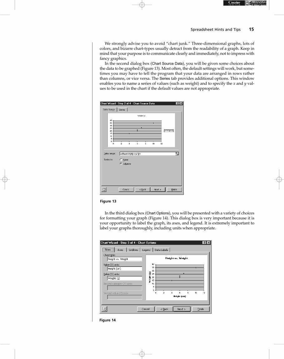
In the second dialog box (Chart Source Data), you will be given some choices aboutthe data to be graphed (Figure 13). Most often, the default settings will work, but some-times you may have to tell the program that your data are arranged in rows ratherthan columns, or vice versa. The Series tab provides additional options. This windowenables you to name a series of values (such as weight) and to specify the x and y val-ues to be used in the chart if the default values are not appropriate.

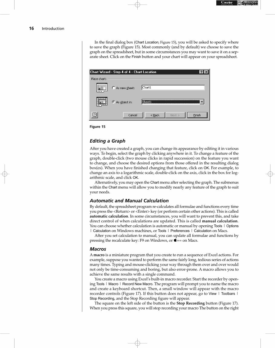
In the third dialog box (Chart Options), you will be presented with a variety of choicesfor formatting your graph (Figure 14). This dialog box is very important because it isyour opportunity to label the graph, its axes, and legend. It is extremely important tolabel your graphs thoroughly, including units when appropriate.

Spreadsheet Hints and Tips 15

Figure 14

Figure 13

In the final dialog box (Chart Location; Figure 15), you will be asked to specify whereto save the graph (Figure 15). Most commonly (and by default) we choose to save thegraph on the spreadsheet, but in some circumstances you may want to save it on a sep-arate sheet. Click on the Finish button and your chart will appear on your spreadsheet.

Editing a Graph

After you have created a graph, you can change its appearance by editing it in variousways. To begin, select the graph by clicking anywhere in it. To change a feature of thegraph, double-click (two mouse clicks in rapid succession) on the feature you wantto change, and choose the desired options from those offered in the resulting dialogbox(es). When you have finished changing that feature, click on OK. For example, tochange an axis to a logarithmic scale, double-click on the axis, click in the box for log-arithmic scale, and click OK.

Alternatively, you may open the Chart menu after selecting the graph. The submenuswithin the Chart menu will allow you to modify nearly any feature of the graph to suityour needs.

Automatic and Manual CalculationBy default, the spreadsheet program re-calculates all formulae and functions every timeyou press the <Return> or <Enter> key (or perform certain other actions). This is calledautomatic calculation. In some circumstances, you will want to prevent this, and takedirect control of when calculations are updated. This is called manual calculation.You can choose whether calculation is automatic or manual by opening Tools | Options| Calculation on Windows machines, or Tools | Preferences | Calculation on Macs.

After you set calculation to manual, you can update all formulae and functions bypressing the recalculate key: F9 on Windows, or += on Macs.

MacrosA macro is a miniature program that you create to run a sequence of Excel actions. Forexample, suppose you wanted to perform the same fairly long, tedious series of actionsmany times. Typing and mouse-clicking your way through them over and over wouldnot only be time-consuming and boring, but also error-prone. A macro allows you toachieve the same results with a single command.

You create a macro using Excel’s built-in macro recorder. Start the recorder by open-ing Tools | Macro | Record New Macro. The program will prompt you to name the macroand create a keyboard shortcut. Then, a small window will appear with the macrorecorder controls (Figure 17). If this button does not appear, go to View | Toolbars |Stop Recording, and the Stop Recording figure will appear.

The square on the left side of the button is the Stop Recording button (Figure 17).When you press this square, you will stop recording your macro The button on the right

16 Introduction

Figure 15

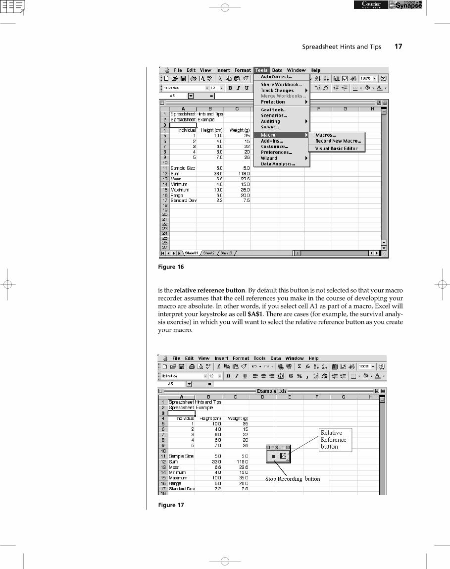
is the relative reference button. By default this button is not selected so that your macrorecorder assumes that the cell references you make in the course of developing yourmacro are absolute. In other words, if you select cell A1 as part of a macro, Excel willinterpret your keystroke as cell $A$1. There are cases (for example, the survival analy-sis exercise) in which you will want to select the relative reference button as you createyour macro.

Spreadsheet Hints and Tips 17

Figure 16

Figure 17

From this point on, Excel will record every action you take. Carry out the entiresequence of operations you want the spreadsheet to do, and then press the Stop Record-ing button in the macro recorder control window. The program will mimic that entiresequence of actions whenever you press the shortcut key or issue the macro command.

Obviously, planning pays off when recording a macro. If you’re creating your ownmacro, go through the sequence of actions at least once in preparation to make sure itactually achieves the desired result. Write down each action, so that you can repeatand record them correctly. If you’re following our instructions to create a macro, be care-ful to execute each step precisely as given. Remember, the computer doesn’t know whatyou want to do; it records everything faithfully, mistakes and all.

Exercise 2, “Spreadsheet Functions and Macros,” provides exercises to help you mas-ter creating macros.

GLOSSARY OF TERMS AND SYMBOLSAbsolute address A cell address (see Cell address) that refers to a specific loca-

tion in the spreadsheet, regardless of its position relative to the selected cell(see p. 12). An absolute address does not change if copied to a new loca-tion. In Excel, an absolute address is indicated by preceding the column let-ter or row number (or both) by a dollar sign ($).

Cell address The location of a cell in the spreadsheet. The cell address consists ofa letter representing the column and a number representing the row (see p.5). Addresses may be relative (see Relative address) or absolute (seeAbsolute address).

Formula A symbolic representation of a set of operations to be carried out by thespreadsheet (see p. 7). Usually, a formula contains one or more celladdresses and one or more mathematical operations to be carried out onthe contents of those cells. The result of the operation(s) appears in the cellin which the formula is entered. In Excel, formulae begin with the equalsign (=).

Function A prewritten formula or set of formulae (see p. 9). Enter a function bytyping it in, by opening Insert | Function and choosing from the list, or byclicking the Paste Function button (fx) and choosing from the list. In Excel,functions begin with the equal sign (=).

Literal Text or a number that is not interpreted or manipulated by the spread-sheet program (see p. 5). Row labels, column labels, and model constantsare literals. To force the program to treat an entry as a literal, begin it withan apostrophe (‘).

Macro A sequence of commands to be executed automatically (see p. 16).Relative address A cell address that refers to a location in the spreadsheet relative

to the position of the selected cell (see p. 12). A relative address changes ifcopied to a new location, preserving the original relationship. Cell address-es are relative by default in Excel, and require no special symbol.

Series A column or row of values in sequence. Most frequently these will be asimple linear series (0, 1, 2, 3, …). See p. 12 for shortcuts to enter a series.

* In a formula, the asterisk (*) represents multiplication. In text, it represents awildcard: a stand-in for any letter or digit.

$ In a cell address, the dollar sign ($) indicates that the following column orrow reference is absolute rather than relative. See Cell address, Absoluteaddress, and Relative address.

^ In a formula, the carat (^) represents exponentiation. That is, 3^2 is equiva-lent to 32.

18 Introduction