EC4440.MPF -Section 0008/29/12 1

00 00 –– FIR Filtering Results ReviewFIR Filtering Results Review

& Practical Applications & Practical Applications

• [p. 2] Mean square signal estimation principles• [p. 3] Orthogonality principle• [p. 6] FIR Wiener filtering concepts• [p.10] FIR Wiener filter equations• [p. 12] Wiener Predictor • [p. 16] Examples• [p. 24] Link between information signal and predictor behaviors• [p. 27] Examples• [p. 37] FIR Weiner filter and error surfaces• [p. 43] Application: Channel equalization• [p. 52] Application: Noise cancellation • [p. 56] Application: Noise cancellation with information leakage• [p. 59] Application: Spatial filtering• [p. 66] Appendices• [p. 70] References

EC4440.MPF -Section 0008/29/12 22

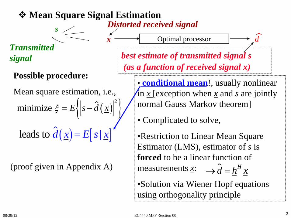
Distorted received signalOptimal processor dx

best estimate of transmitted signal s (as a function of received signal x)

s

Transmitted signal

Possible procedure:

Mean square estimation, i.e.,• conditional mean!, usually nonlinear in x [exception when x and s are jointly normal Gauss Markov theorem]

• Complicated to solve,

•Restriction to Linear Mean Square Estimator (LMS), estimator of s is forced to be a linear function of measurements x:

•Solution via Wiener Hopf equations using orthogonality principle

( ){ }2minimize E s d xξ = −

( ) [ ]leads to |d x E s x=

Mean Square Signal Estimation

Hd h x→ =(proof given in Appendix A)

EC4440.MPF -Section 0008/29/12 3

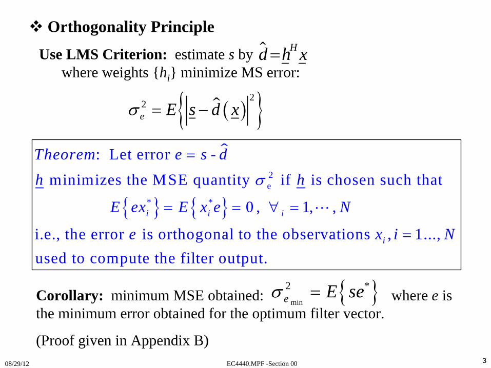
Corollary: minimum MSE obtained: where e is the minimum error obtained for the optimum filter vector.

(Proof given in Appendix B)3

( ){ }22e E s d xσ = −

Use LMS Criterion: estimate s by where weights {hi } minimize MS error:

Hd h x=

{ }min

2 *e E seσ =

Orthogonality Principle

{ } { }2e

* *

: Let error - minimizes the MSE quantity if is chosen such that

0 , 1, ,

i.e., the error is orthogonal to the observations , 1...,used to compute

i i i

i

Theorem e s dh h

E ex E x e N

e x i N

σ

=

= = ∀ =

=

the filter output.

EC4440.MPF -Section 0008/29/12 44

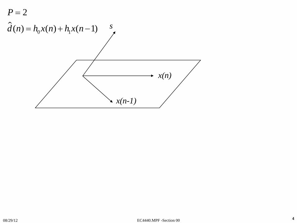
x(n-1)

s

x(n)

0 1

2

( ) ( ) ( 1)

P

d n h x n h x n

=

= + −

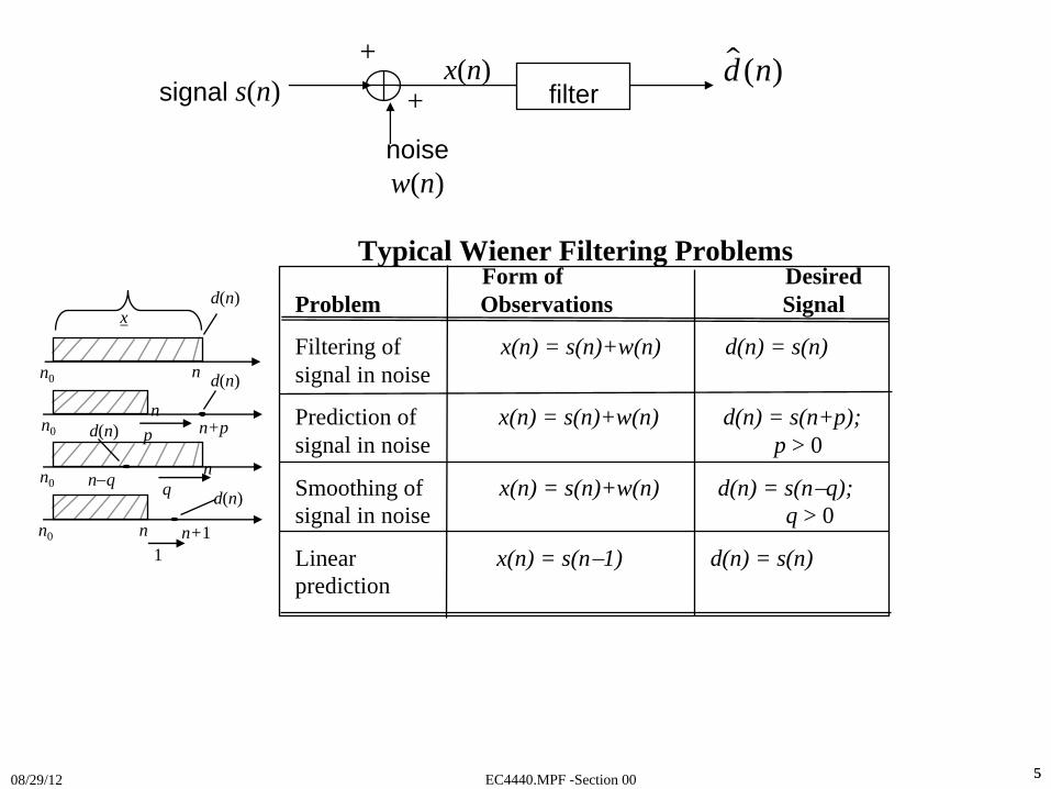
EC4440.MPF -Section 0008/29/12 55

Form of Desired Problem Observations Signal

Filtering of x(n) = s(n)+w(n) d(n) = s(n) signal in noise

Prediction of x(n) = s(n)+w(n) d(n) = s(n+p); signal in noise p > 0

Smoothing of x(n) = s(n)+w(n) d(n) = s(n−q); signal in noise q > 0

Linear x(n) = s(n−1) d(n) = s(n) prediction

Typical Wiener Filtering Problems

n0

n0

n0

n0

d(n)

d(n)

d(n)

d(n)

n

n

n

n

x

n+1

n+p

n−q q

p

1

signal s(n) filter

noise w(n)

x(n) ( )d n+

+

EC4440.MPF -Section 0008/29/12 66

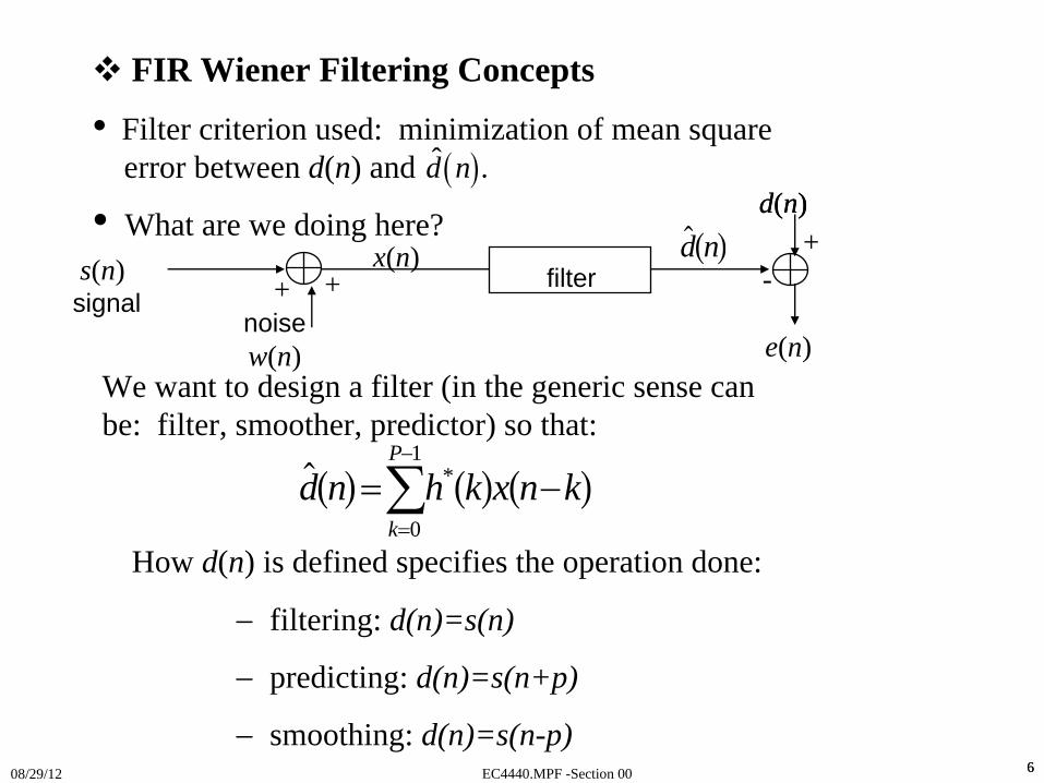
FIR Wiener Filtering Concepts

• Filter criterion used: minimization of mean square error between d(n) and

• What are we doing here?

( )ˆ .d n

We want to design a filter (in the generic sense can be: filter, smoother, predictor) so that:

*d n h k x n kk

P

a f a f a f= −=

−

∑0

1

How d(n) is defined specifies the operation done:

−

filtering: d(n)=s(n)

−

predicting: d(n)=s(n+p)

−

smoothing: d(n)=s(n-p)

s(n) signal

filter

noise w(n)

x(n)

d(n)d na f

e(n)

d(n)+

-++

EC4440.MPF -Section 0008/29/12 77

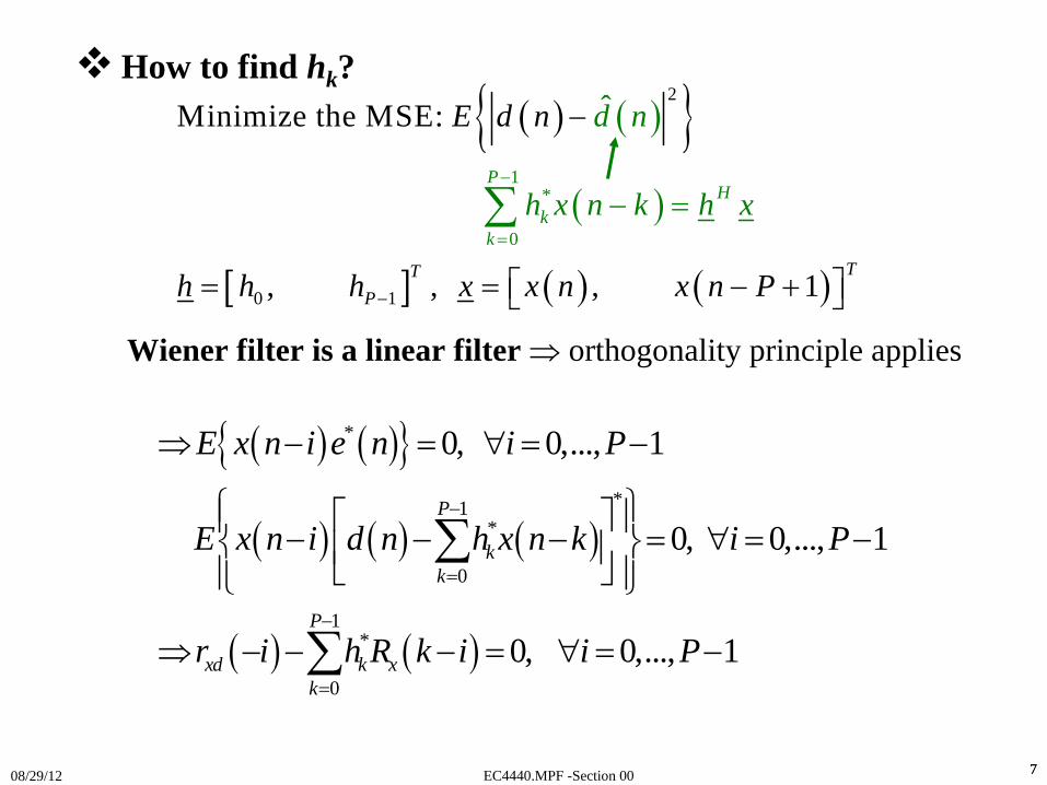
How to find hk?( ) ( ){ }

( )

[ ] ( ) ( )

2

0 1

1*

0

ˆ

Minimize the MSE:

, , , 1

PH

kk

TTP

dE d n

h h h x x n

n

h x n

P

x

x n

k h−

=

−

−

= = − +

− =

⎡ ⎤⎣ ⎦

∑

Wiener filter is a linear filter ⇒ orthogonality principle applies

( ) ( ){ }

( ) ( ) ( )

( ) ( )

*

*1*

0

1*

0

0, 0,..., 1

0, 0,..., 1

0, 0,..., 1

P

kk

P

xd k xk

E x n i e n i P

E x n i d n h x n k i P

r i h R k i i P

−

=

−

=

⇒ − = ∀ = −

⎧ ⎫⎡ ⎤⎪ ⎪− − − = ∀ = −⎨ ⎬⎢ ⎥⎣ ⎦⎪ ⎪⎩ ⎭

⇒ − − − = ∀ = −

∑

∑

EC4440.MPF -Section 0008/29/12 88

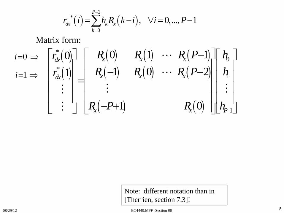
Matrix form:

( )( )

( ) ( ) ( )( ) ( ) ( )

( ) ( )

*0

*1

1

0 1 101 0 21

1 0

x x xdx

x x xdx

x x P

R R R P hrR R R P hr

R P R h −

−⎡ ⎤⎡ ⎤ ⎡ ⎤⎢ ⎥⎢ ⎥ ⎢ ⎥− −⎢ ⎥⎢ ⎥ ⎢ ⎥=⎢ ⎥⎢ ⎥ ⎢ ⎥⎢ ⎥⎢ ⎥ ⎢ ⎥− +⎢ ⎥⎣ ⎦⎣ ⎦ ⎣ ⎦

0i= ⇒

1i = ⇒

Note: different notation than in [Therrien, section 7.3]!

( ) ( )1

*

0

, 0,..., 1P

dx k xk

r i h R k i i P−

=

= − ∀ = −∑

EC4440.MPF -Section 0008/29/12 99

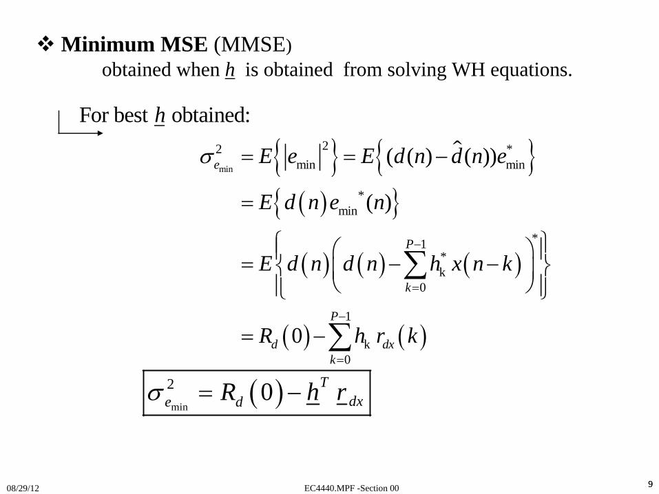
Minimum MSE (MMSE)obtained when h is obtained from solving WH equations.

{ } { }( ){ }

( ) ( ) ( )

( ) ( )

min

22 *min min

*min

*1*k

0

1

k0

For best obtained:

( ( ) ( ))

( )

0

e

P

k

P

d dxk

h

E e E d n d n e

E d n e n

E d n d n h x n k

R h r k

σ

−

=

−

=

= = −

=

⎧ ⎫⎛ ⎞⎪ ⎪= − −⎨ ⎬⎜ ⎟⎝ ⎠⎪ ⎪⎩ ⎭

= −

∑

∑

( )min

2 0 Tdxe dR h rσ = −

EC4440.MPF -Section 0008/29/12 1010

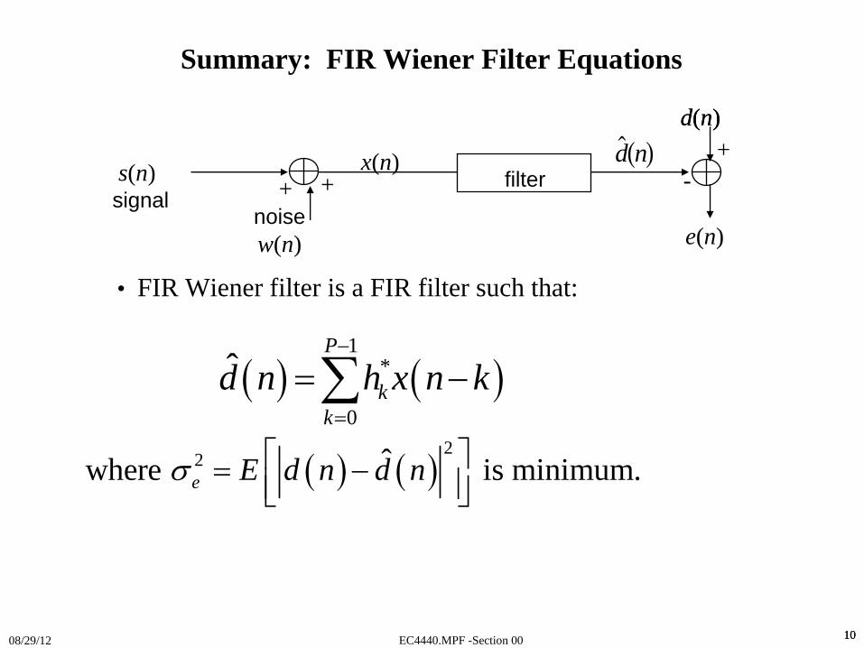
Summary: FIR Wiener Filter Equations

• FIR Wiener filter is a FIR filter such that:

( ) ( )1

*

0

ˆP

kk

d n h x n k−

=

= −∑

( ) ( )2

2 ˆwhere is minimum.e E d n d nσ ⎡ ⎤= −⎢ ⎥⎣ ⎦

s(n) signal

filter

noise w(n)

x(n)

d(n)d na f

e(n)

d(n)+

-++

EC4440.MPF -Section 0008/29/12 1111

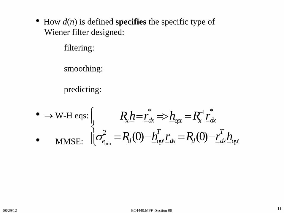
• How d(n) is defined specifies the specific type of Wiener filter designed:

filtering:

smoothing:

predicting:

• → W-H eqs:

• MMSE: min

* *1

2 (0) (0)dx dxoptx x

T Tdx dxopt opte d d

R h r h R r

R h r R r hσ

−⎧ = => =⎪⎨

= − = −⎪⎩

EC4440.MPF -Section 0008/29/12 1212

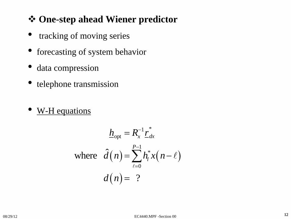
One-step ahead Wiener predictor

• tracking of moving series

• forecasting of system behavior

• data compression

• telephone transmission

• W-H equations

( ) ( )

( )

*1opt

1*

0

ˆwhere

?

dxx

P

l

h R r

d n h x n

d n

−

−

=

=

= −

=

∑

EC4440.MPF -Section 0008/29/12 1313

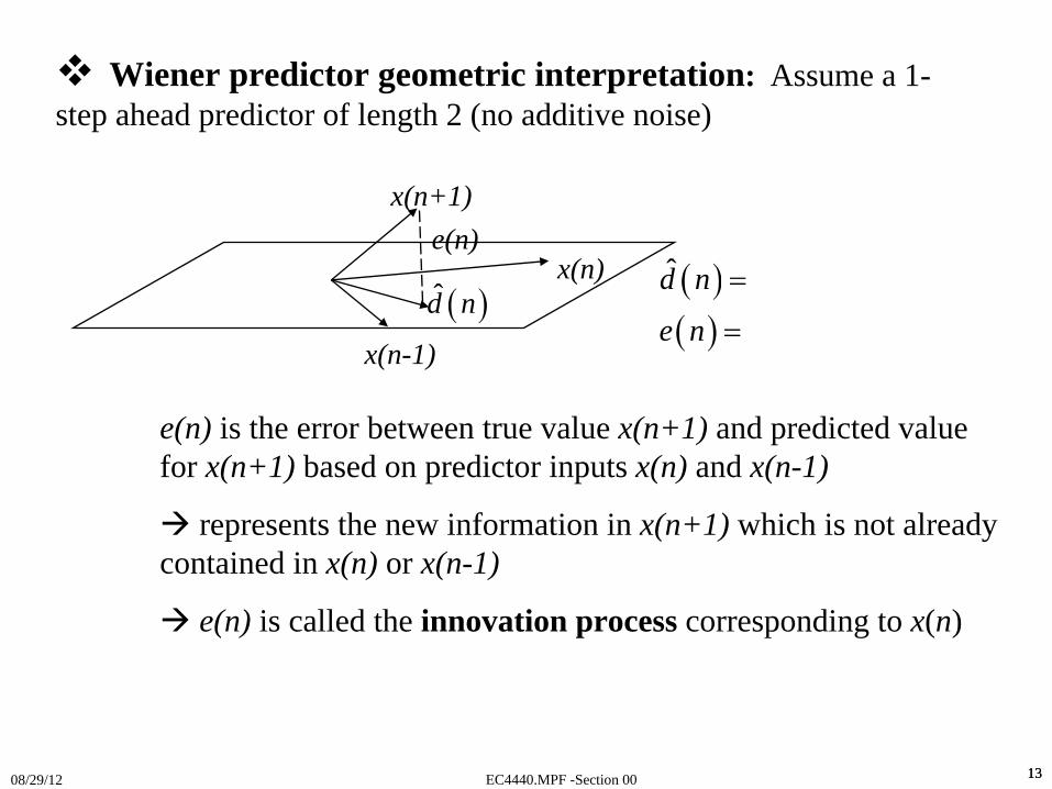
Wiener predictor geometric interpretation: Assume a 1-step ahead predictor of length 2 (no additive noise)

x(n)

x(n+1)

x(n-1)

e(n)( )( )

d̂ n

e n

=

=

e(n) is the error between true value x(n+1) and predicted value for x(n+1) based on predictor inputs x(n) and x(n-1)

represents the new information in x(n+1) which is not already contained in x(n) or x(n-1)

e(n) is called the innovation process corresponding to x(n)

( )d̂ n

EC4440.MPF -Section 0008/29/12 1414

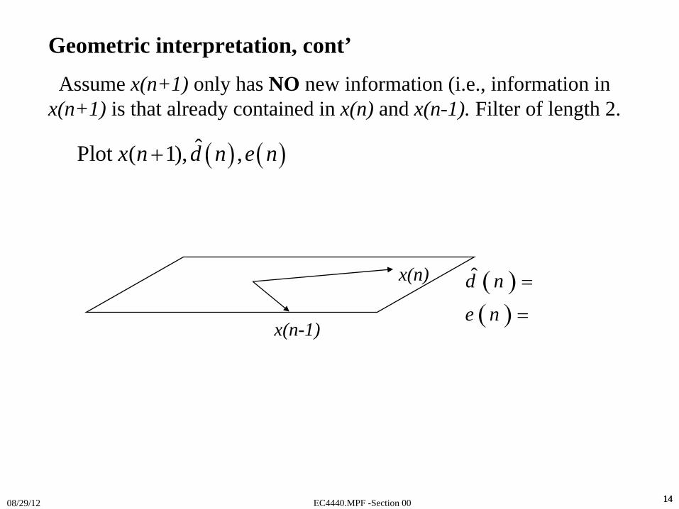
Geometric interpretation, cont’

Assume x(n+1) only has NO new information (i.e., information in x(n+1) is that already contained in x(n) and x(n-1). Filter of length 2.

x(n)

x(n-1)

( )( )

d̂ n

e n

=

=

( ) ( )ˆPlot ( 1), ,x n d n e n+

EC4440.MPF -Section 0008/29/12 1515

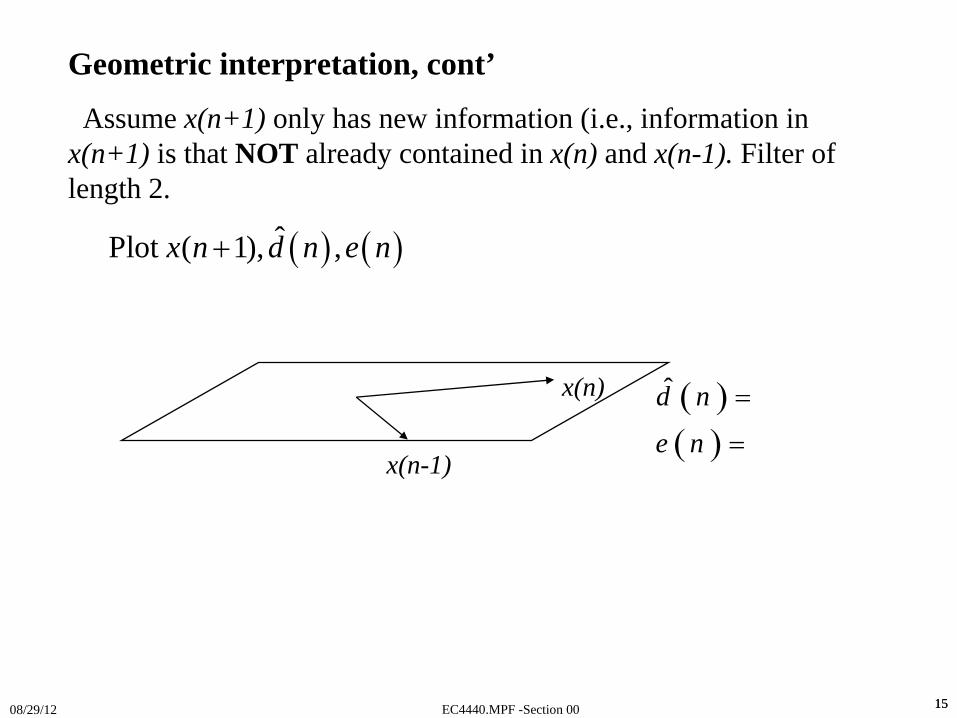
Geometric interpretation, cont’

Assume x(n+1) only has new information (i.e., information in x(n+1) is that NOT already contained in x(n) and x(n-1). Filter of length 2.

x(n)

x(n-1)

( )( )

d̂ n

e n

=

=

( ) ( )ˆPlot ( 1), ,x n d n e n+

EC4440.MPF -Section 0008/29/12 1616

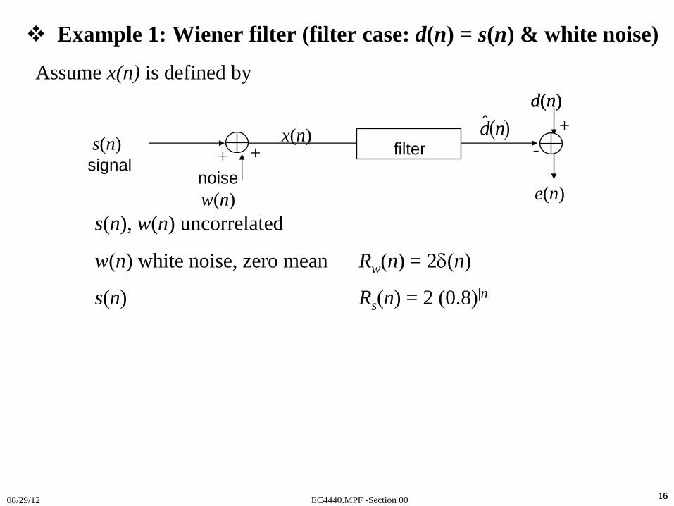
Example 1: Wiener filter (filter case: d(n) = s(n) & white noise)

Assume x(n) is defined by

s(n), w(n) uncorrelated

w(n) white noise, zero mean Rw (n) = 2δ(n)

s(n) Rs (n) = 2 (0.8)|n|

s(n) signal

filter

noise w(n)

x(n)

d(n)d na f

e(n)

d(n)+

-++

EC4440.MPF -Section 0008/29/12 1717

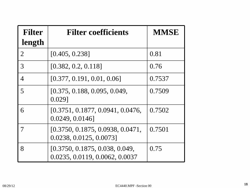
EC4440.MPF -Section 0008/29/12 1818

Filter length

Filter coefficients MMSE

2 [0.405, 0.238] 0.81

3 [0.382, 0.2, 0.118] 0.76

4 [0.377, 0.191, 0.01, 0.06] 0.7537

5 [0.375, 0.188, 0.095, 0.049, 0.029]

0.7509

6 [0.3751, 0.1877, 0.0941, 0.0476, 0.0249, 0.0146]

0.7502

7 [0.3750, 0.1875, 0.0938, 0.0471, 0.0238, 0.0125, 0.0073]

0.7501

8 [0.3750, 0.1875, 0.038, 0.049, 0.0235, 0.0119, 0.0062, 0.0037

0.75

EC4440.MPF -Section 0008/29/12 1919

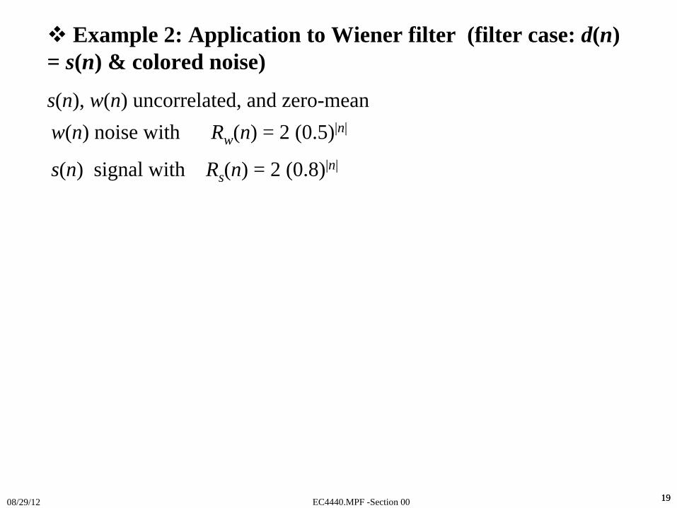
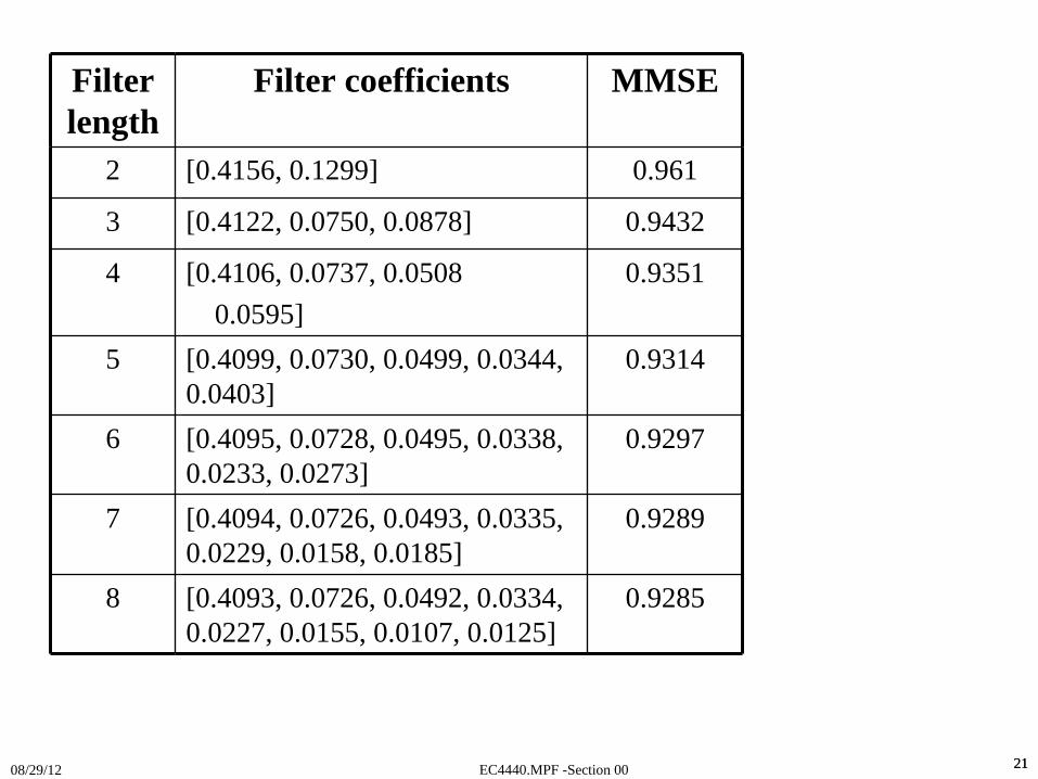
w(n) noise with Rw (n) = 2 (0.5)|n|

s(n) signal with Rs (n) = 2 (0.8)|n|

Example 2: Application to Wiener filter (filter case: d(n) = s(n) & colored noise)

s(n), w(n) uncorrelated, and zero-mean

EC4440.MPF -Section 0008/29/12 2020

EC4440.MPF -Section 0008/29/12 2121

Filter length

Filter coefficients MMSE

2 [0.4156, 0.1299] 0.961

3 [0.4122, 0.0750, 0.0878] 0.9432

4 [0.4106, 0.0737, 0.05080.0595]

0.9351

5 [0.4099, 0.0730, 0.0499, 0.0344, 0.0403]

0.9314

6 [0.4095, 0.0728, 0.0495, 0.0338, 0.0233, 0.0273]

0.9297

7 [0.4094, 0.0726, 0.0493, 0.0335, 0.0229, 0.0158, 0.0185]

0.9289

8 [0.4093, 0.0726, 0.0492, 0.0334, 0.0227, 0.0155, 0.0107, 0.0125]

0.9285

EC4440.MPF -Section 0008/29/12 2222

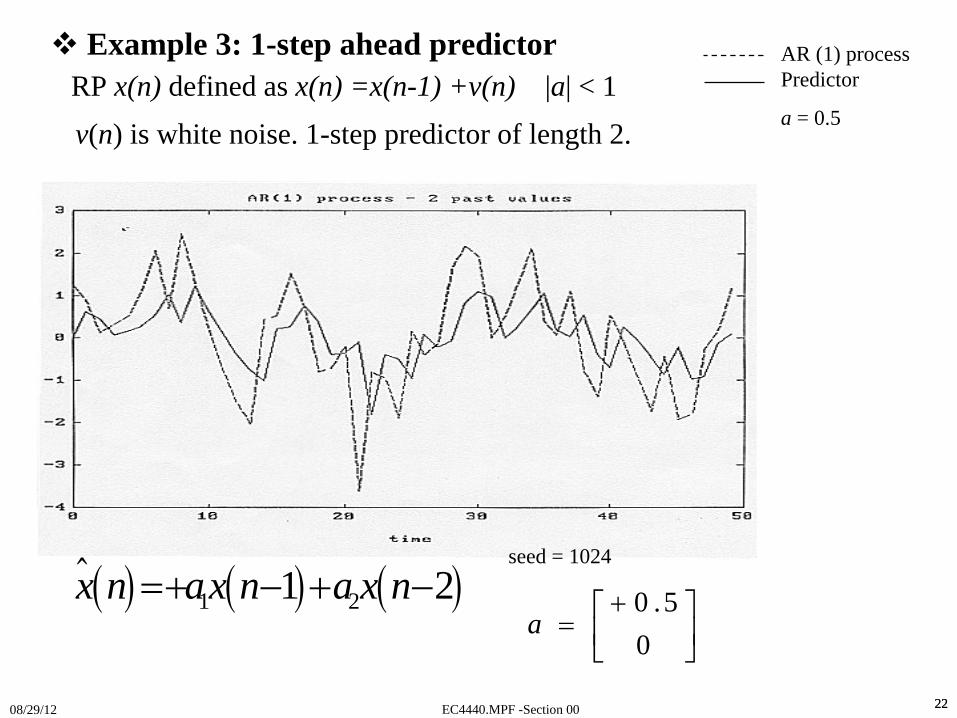
AR (1) process Predictor

a = 0.5

seed = 1024

a =+LNMOQP

0 50

.( ) ( ) ( )1 21 2x n ax n a x n=+ − + −

RP x(n) defined as x(n) =x(n-1) +v(n) |a| < 1v(n) is white noise. 1-step predictor of length 2.

Example 3: 1-step ahead predictor

EC4440.MPF -Section 0008/29/12 23

EC4440.MPF -Section 0008/29/12 2424

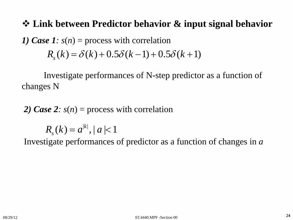
Link between Predictor behavior & input signal behavior

1) Case 1: s(n) = process with correlation

Investigate performances of N-step predictor as a function of changes N

| |( ) , | | 1ksR k a a= <

2) Case 2: s(n) = process with correlation

Investigate performances of predictor as a function of changes in a

( ) ( ) 0.5 ( 1) 0.5 ( 1)sR k k k kδ δ δ= + − + +

EC4440.MPF -Section 0008/29/12 25

( ) ( ) 0.5 ( 1) 0.5 ( 1)sR k k k kδ δ δ= + − + +1) Case 1: s(n) = wss process with

EC4440.MPF -Section 0008/29/12 26

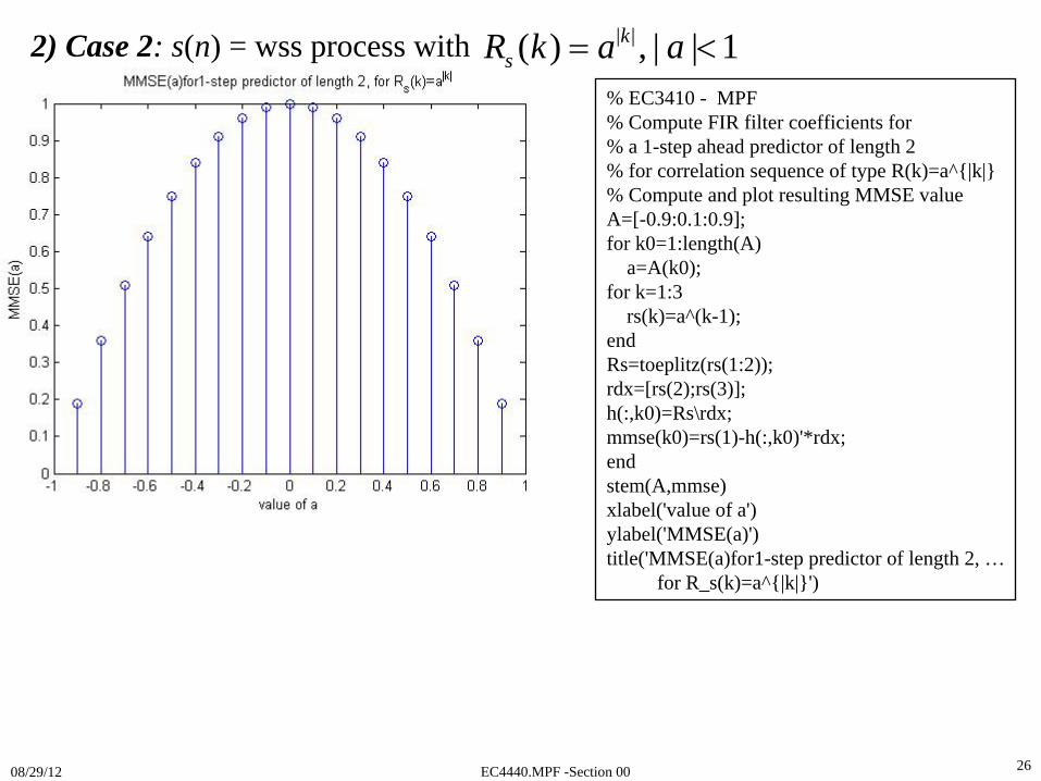
% EC3410 - MPF% Compute FIR filter coefficients for % a 1-step ahead predictor of length 2% for correlation sequence of type R(k)=a^{|k|}% Compute and plot resulting MMSE valueA=[-0.9:0.1:0.9];for k0=1:length(A)

a=A(k0);for k=1:3

rs(k)=a^(k-1);endRs=toeplitz(rs(1:2));rdx=[rs(2);rs(3)];h(:,k0)=Rs\rdx;mmse(k0)=rs(1)-h(:,k0)'*rdx;endstem(A,mmse)xlabel('value of a')ylabel('MMSE(a)')title('MMSE(a)for1-step predictor of length 2, …

for R_s(k)=a^{|k|}')

2) Case 2: s(n) = wss process with | |( ) , | | 1ksR k a a= <

EC4440.MPF -Section 0008/29/12 2727

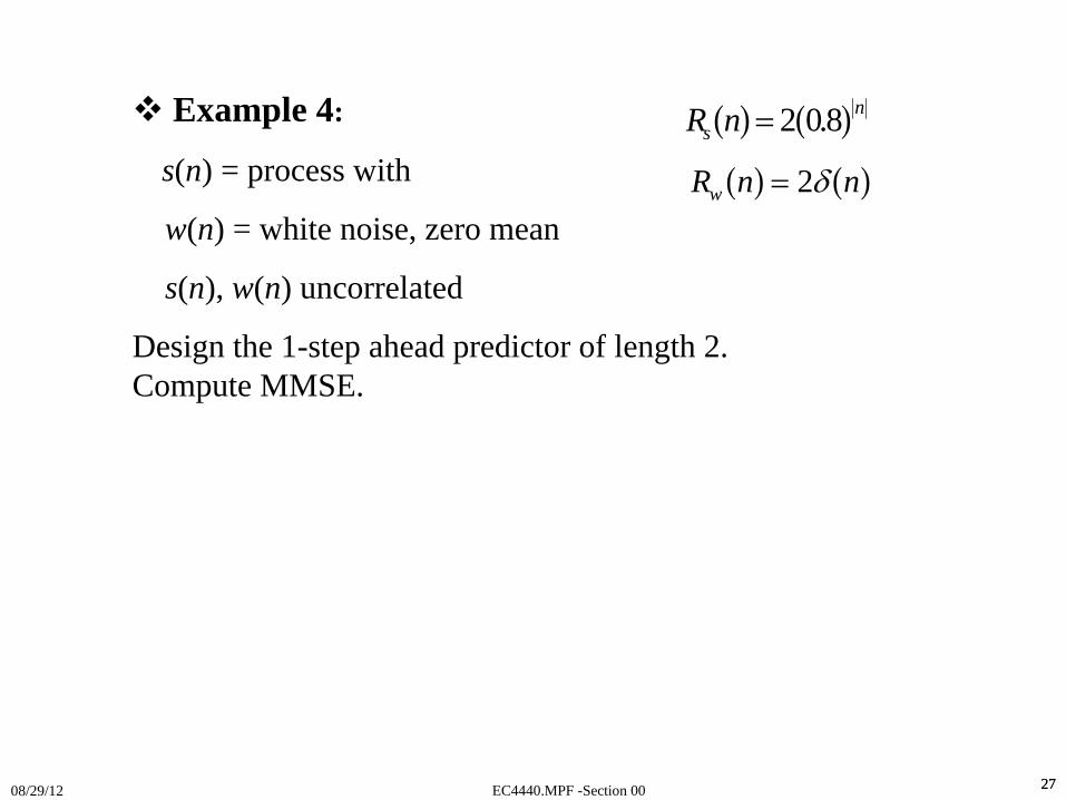
Example 4:

s(n) = process with

w(n) = white noise, zero mean

s(n), w(n) uncorrelated

Design the 1-step ahead predictor of length 2. Compute MMSE.

R nsna f a f= 2 08.

R n nw a f a f= 2δ

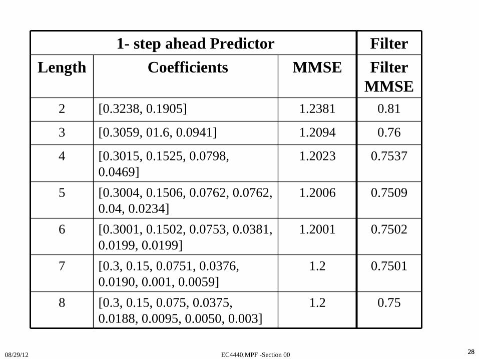
EC4440.MPF -Section 0008/29/12 2828

1- step ahead Predictor FilterLength Coefficients MMSE Filter

MMSE2 [0.3238, 0.1905] 1.2381 0.81

3 [0.3059, 01.6, 0.0941] 1.2094 0.76

4 [0.3015, 0.1525, 0.0798, 0.0469]

1.2023 0.7537

5 [0.3004, 0.1506, 0.0762, 0.0762, 0.04, 0.0234]

1.2006 0.7509

6 [0.3001, 0.1502, 0.0753, 0.0381, 0.0199, 0.0199]

1.2001 0.7502

7 [0.3, 0.15, 0.0751, 0.0376, 0.0190, 0.001, 0.0059]

1.2 0.7501

8 [0.3, 0.15, 0.075, 0.0375, 0.0188, 0.0095, 0.0050, 0.003]

1.2 0.75

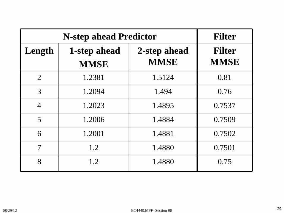
EC4440.MPF -Section 0008/29/12 2929

N-step ahead Predictor FilterLength 1-step ahead

MMSE2-step ahead

MMSEFilter

MMSE2 1.2381 1.5124 0.81

3 1.2094 1.494 0.76

4 1.2023 1.4895 0.7537

5 1.2006 1.4884 0.7509

6 1.2001 1.4881 0.7502

7 1.2 1.4880 0.7501

8 1.2 1.4880 0.75

EC4440.MPF -Section 0008/29/12 3030

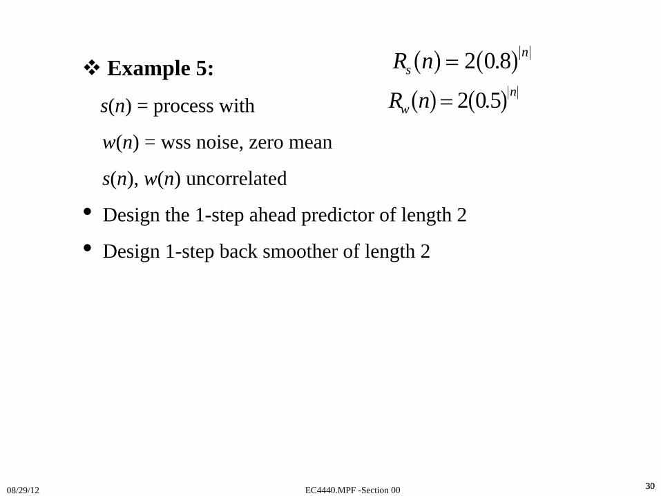
Example 5:

s(n) = process with

w(n) = wss noise, zero mean

s(n), w(n) uncorrelated

• Design the 1-step ahead predictor of length 2

• Design 1-step back smoother of length 2

R nsna f a f= 2 0 8.

R nwna f a f= 2 0 5.

EC4440.MPF -Section 0008/29/12 3131

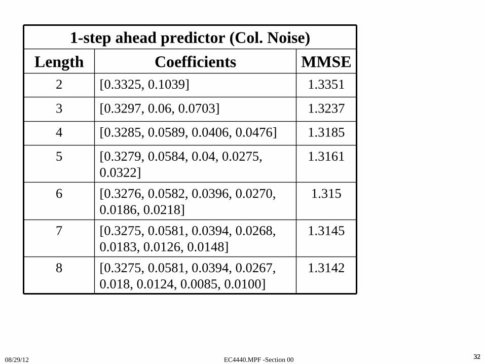
EC4440.MPF -Section 0008/29/12 3232

1-step ahead predictor (Col. Noise)Length Coefficients MMSE

2 [0.3325, 0.1039] 1.3351

3 [0.3297, 0.06, 0.0703] 1.3237

4 [0.3285, 0.0589, 0.0406, 0.0476] 1.3185

5 [0.3279, 0.0584, 0.04, 0.0275, 0.0322]

1.3161

6 [0.3276, 0.0582, 0.0396, 0.0270, 0.0186, 0.0218]

1.315

7 [0.3275, 0.0581, 0.0394, 0.0268, 0.0183, 0.0126, 0.0148]

1.3145

8 [0.3275, 0.0581, 0.0394, 0.0267, 0.018, 0.0124, 0.0085, 0.0100]

1.3142

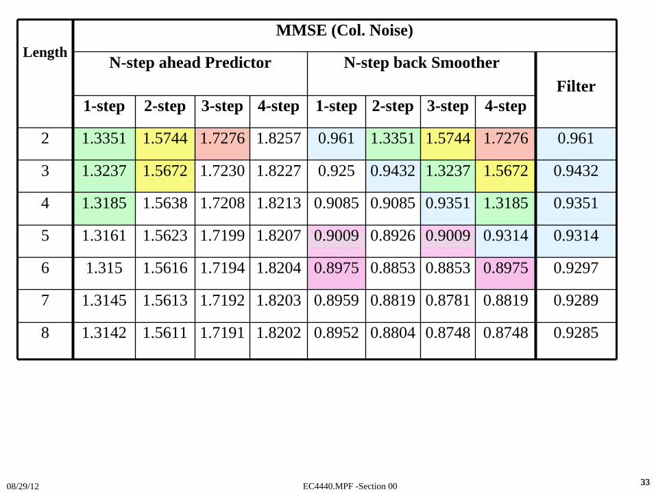
EC4440.MPF -Section 0008/29/12 3333

LengthMMSE (Col. Noise)

N-step ahead Predictor N-step back SmootherFilter

1-step 2-step 3-step 4-step 1-step 2-step 3-step 4-step

2 1.3351 1.5744 1.7276 1.8257 0.961 1.3351 1.5744 1.7276 0.961

3 1.3237 1.5672 1.7230 1.8227 0.925 0.9432 1.3237 1.5672 0.9432

4 1.3185 1.5638 1.7208 1.8213 0.9085 0.9085 0.9351 1.3185 0.9351

5 1.3161 1.5623 1.7199 1.8207 0.9009 0.8926 0.9009 0.9314 0.9314

6 1.315 1.5616 1.7194 1.8204 0.8975 0.8853 0.8853 0.8975 0.9297

7 1.3145 1.5613 1.7192 1.8203 0.8959 0.8819 0.8781 0.8819 0.9289

8 1.3142 1.5611 1.7191 1.8202 0.8952 0.8804 0.8748 0.8748 0.9285

EC4440.MPF -Section 0008/29/12 3434

Comments

EC4440.MPF -Section 0008/29/12 3535

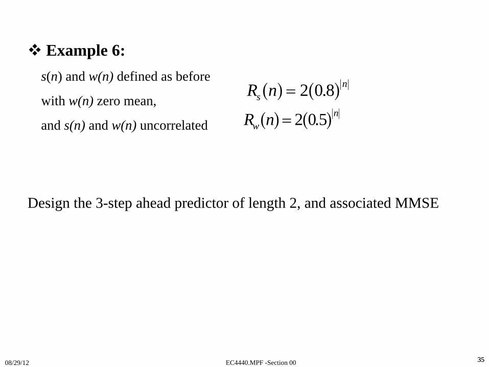
Example 6:s(n) and w(n) defined as before

with w(n) zero mean,

and s(n) and w(n) uncorrelated

Design the 3-step ahead predictor of length 2, and associated MMSE

R nsna f a f= 2 0 8.

R nwna f a f= 2 0 5.

EC4440.MPF -Section 0008/29/12 36

EC4440.MPF -Section 0008/29/12 37

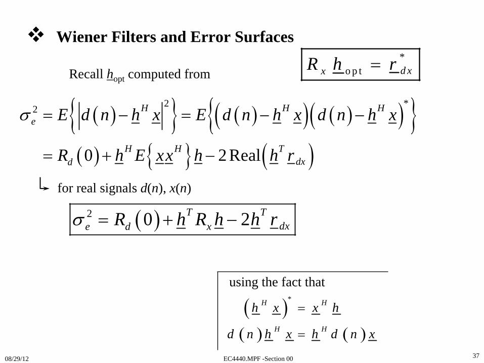
Wiener Filters and Error Surfaces*

o p t d xxR h r=Recall hopt computed from

( ){ } ( )( ) ( )( ){ }( ) { } ( )

*22

0 2 Real

H H He

H H Tdxd

E d n h x E d n h x d n h x

R h E xx h h r

σ = − = − −

= + −

for real signals d(n), x(n)

( )2 0 2T Tdxe d xR h R h h rσ = + −

using the fact that

( )( ) ( )

*H H

H H

h x x h

d n h x h d n x

=

=

EC4440.MPF -Section 0008/29/12 38

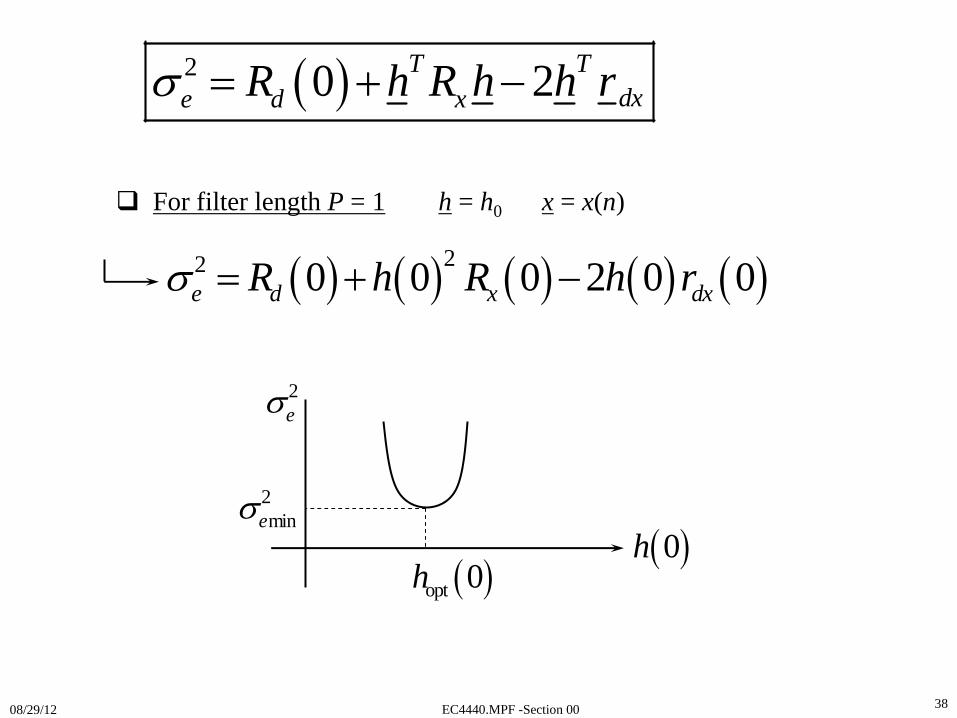
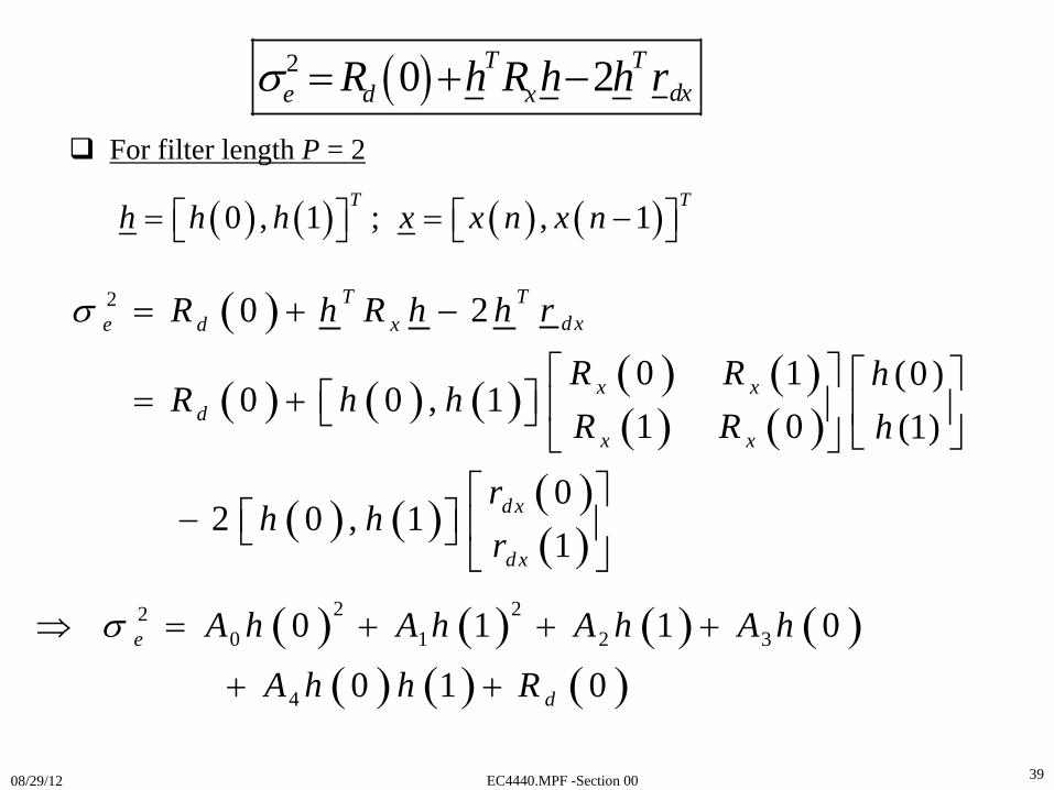
For filter length P = 1 h = h0 x = x(n)

( ) ( ) ( ) ( ) ( )22 0 0 0 2 0 0e d x dxR h R h rσ = + −

2eσ

2mineσ

( )0h( )opt 0h

( )2 0 2T Tdxe d xR h R h h rσ = + −

EC4440.MPF -Section 0008/29/12 39

For filter length P = 2

( )

( ) ( ) ( ) ( ) ( )( ) ( )

( ) ( ) ( )( )

2 0 2

0 1 (0 )0 0 , 1

1 0 (1)

02 0 , 1

1

T Td xe d x

x xd

x x

d x

d x

R h R h h r

R R hR h h

R R h

rh h

r

σ = + −

⎡ ⎤ ⎡ ⎤= + ⎡ ⎤ ⎢ ⎥ ⎢ ⎥⎣ ⎦

⎣ ⎦⎣ ⎦⎡ ⎤

− ⎡ ⎤ ⎢ ⎥⎣ ⎦⎣ ⎦

( ) ( ) ( ) ( )0 , 1 ; , 1T T

h h h x x n x n= = −⎡ ⎤ ⎡ ⎤⎣ ⎦ ⎣ ⎦

( ) ( ) ( ) ( )( ) ( ) ( )

2 220 1 2 3

4

0 1 1 0

0 1 0e

d

A h A h A h A h

A h h R

σ⇒ = + + +

+ +

( )2 0 2T Tdxe d xR h R h h rσ = + −

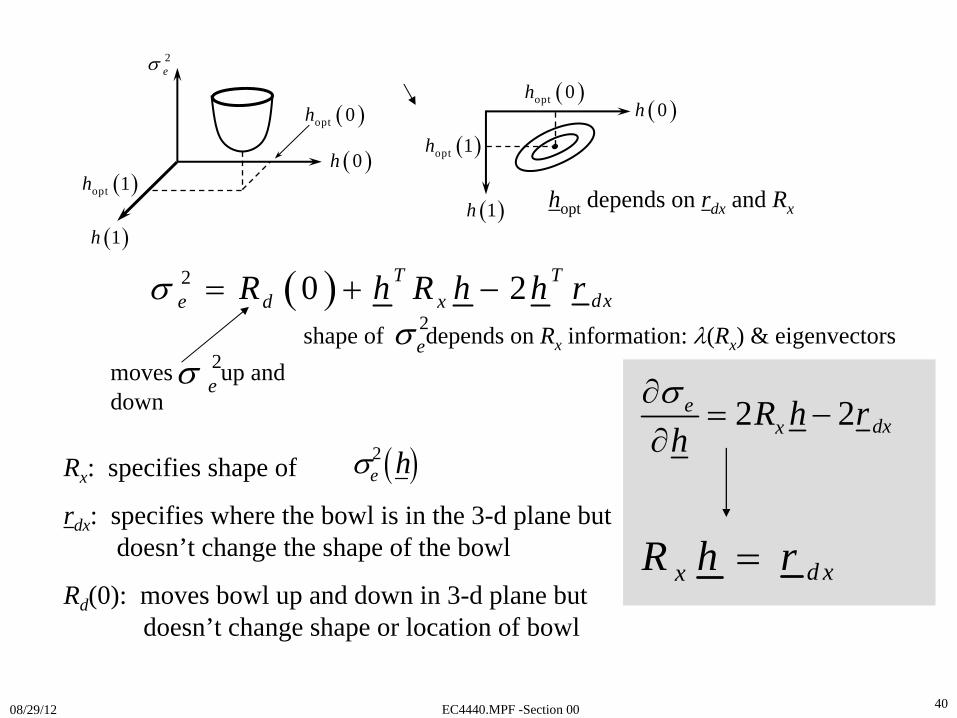
EC4440.MPF -Section 0008/29/12 40

shape of depends on Rx information: λ(Rx ) & eigenvectors

( )2 0 2T Tdxe d xR h R h h rσ = + −

moves up and down

hopt depends on rdx and Rx

2eσ

2eσ

2 2edxxR h r

hσ∂

= −∂

d xxR h r=

Rx : specifies shape of

rdx : specifies where the bowl is in the 3-d plane but doesn’t change the shape of the bowl

Rd (0): moves bowl up and down in 3-d plane but doesn’t change shape or location of bowl

( )2e hσ

2eσ

( )0h

( )opt 0h

( )1h

( )opt 1h

( )0h( )opt 0h

( )1h

( )opt 1h

EC4440.MPF -Section 0008/29/12 41

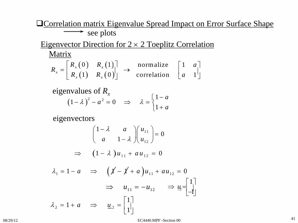
Correlation matrix Eigenvalue Spread Impact on Error Surface Shapesee plots

Eigenvector Direction for 2 ×

2 Toeplitz Correlation Matrix

( ) ( )( ) ( )0 1 normalize 11 0 correlation 1

x xx

x x

R R aR

R R a⎡ ⎤ ⎡ ⎤

= →⎢ ⎥ ⎢ ⎥⎣ ⎦⎣ ⎦

eigenvalues of Rx

( )2 2 11 0

1a

aa

λ λ−⎧

− − = ⇒ = ⎨ +⎩eigenvectors

11

12

10

1uaua

λλ

− ⎛ ⎞⎛ ⎞=⎜ ⎟⎜ ⎟−⎝ ⎠ ⎝ ⎠

1 1 1aλ = − ⇒ 1−( ) 11 12 0a u au+ + =

( ) 1 1 1 21 0u a uλ⇒ − + =

11 12u u⇒ = − 1

11

u⎡ ⎤

⇒ =⎢ ⎥−⎣ ⎦

22

11

1a uλ

⎡ ⎤= + ⇒ = ⎢ ⎥

⎣ ⎦

EC4440.MPF -Section 0008/29/12 42

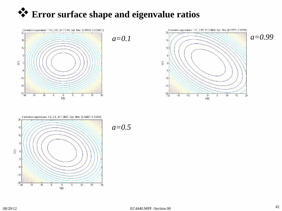
Error surface shape and eigenvalue ratios

a=0.1

a=0.5

a=0.99

EC4440.MPF -Section 0008/29/12 4343

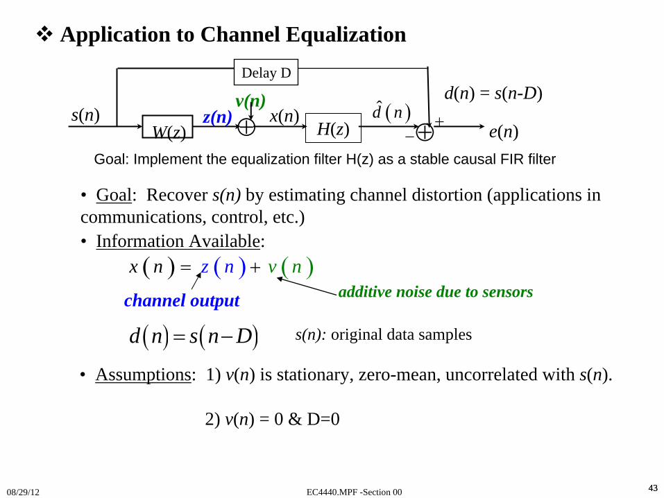
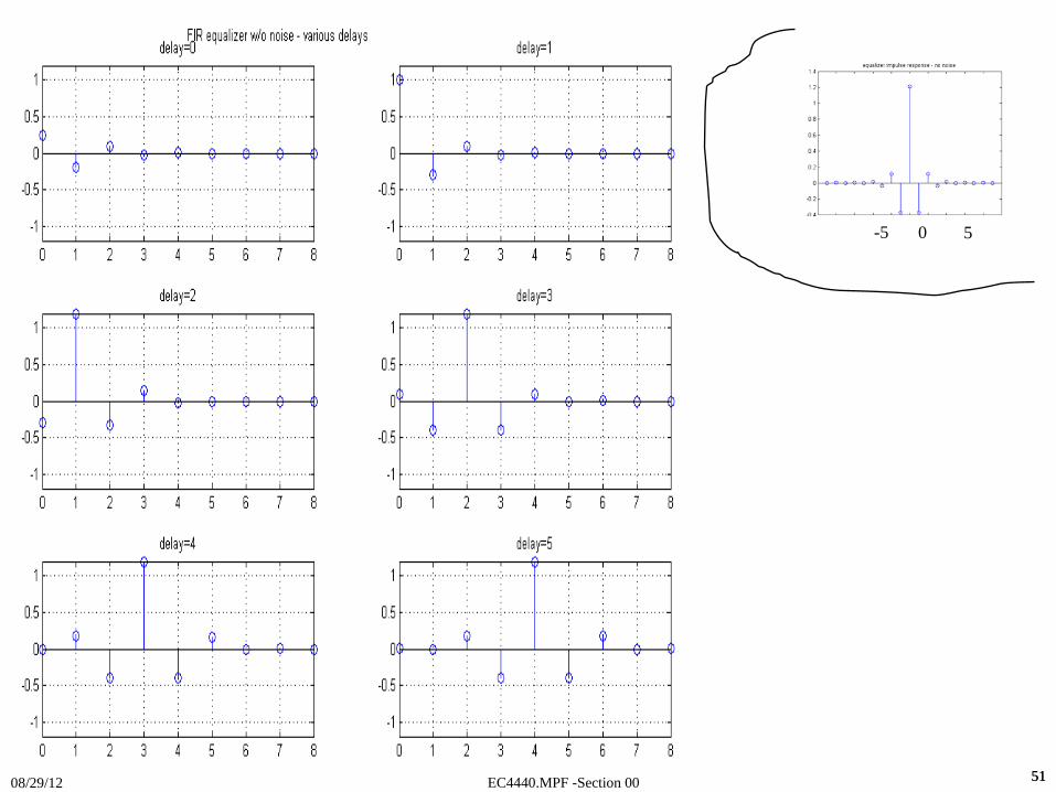
• Goal: Recover s(n) by estimating channel distortion (applications in communications, control, etc.)

Goal: Implement the equalization filter H(z) as a stable causal FIR filter

• Assumptions: 1) v(n) is stationary, zero-mean, uncorrelated with s(n).

• Information Available: ( ) ( ) ( )x n vz n n= +

channel output additive noise due to sensors

( ) ( )d n s n D= − s(n): original data samples

2) v(n) = 0 & D=0

Application to Channel EqualizationDelay D

d(n) = s(n-D)s(n)

v(n)H(z)

z(n)e(n)

( )d̂ n⊕

x(n)⊕ +−W(z)

EC4440.MPF -Section 0008/29/12 4444

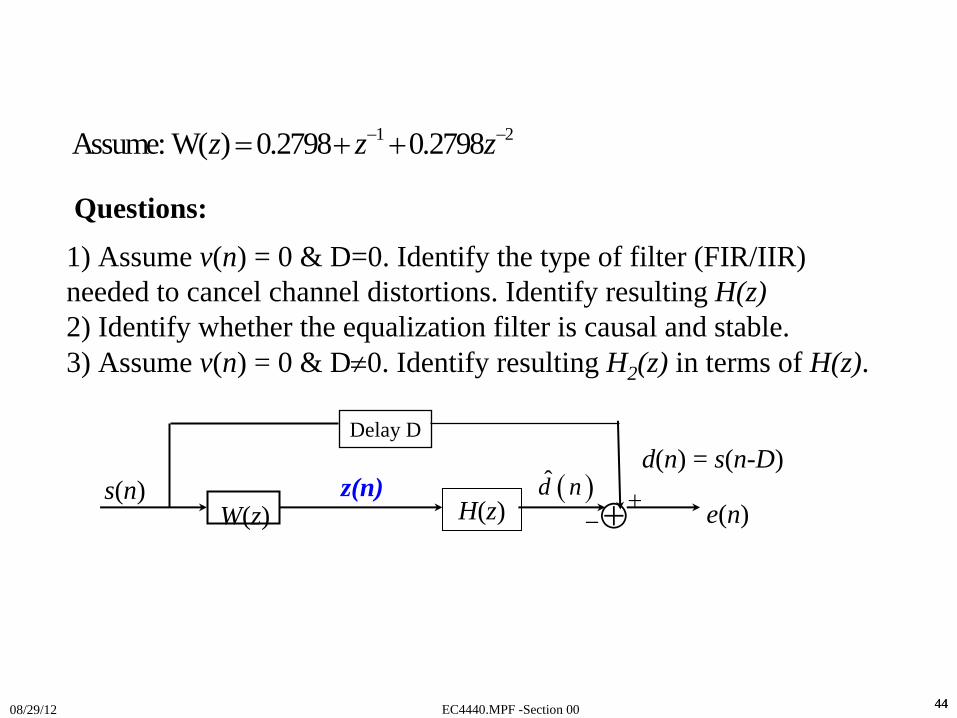
1 2Assume: W( ) 0.2798 0.2798z z z− −= + +

1) Assume v(n) = 0 & D=0. Identify the type of filter (FIR/IIR) needed to cancel channel distortions. Identify resulting H(z)2) Identify whether the equalization filter is causal and stable.3) Assume v(n) = 0 & D≠0. Identify resulting H2 (z) in terms of H(z).

Questions:

d(n) = s(n-D)s(n)

H(z)z(n)

e(n)( )d̂ n

⊕+−W(z)

Delay D

EC4440.MPF -Section 0008/29/12 45

EC4440.MPF -Section 0008/29/12 46

EC4440.MPF -Section 0008/29/12 47

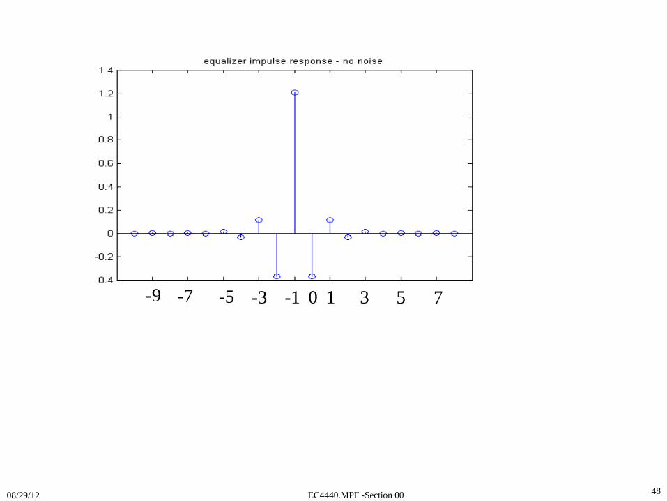
EC4440.MPF -Section 0008/29/12 48

-1 0 1-3 3 5-5-7 7-9

EC4440.MPF -Section 0008/29/12 49

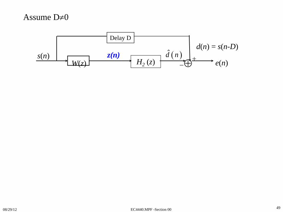
d(n) = s(n-D)s(n)

H2 (z)z(n)

e(n)( )d̂ n

⊕+−W(z)

Delay D

Assume D≠0

EC4440.MPF -Section 0008/29/12 50

EC4440.MPF -Section 0008/29/12 5151

0 5-5

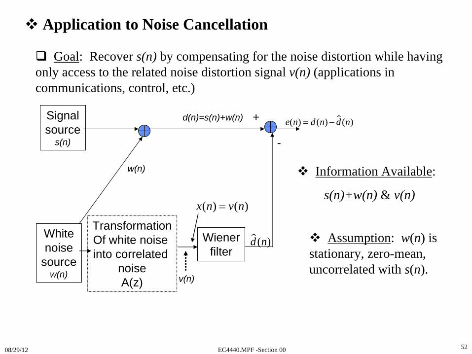
EC4440.MPF -Section 0008/29/12 52

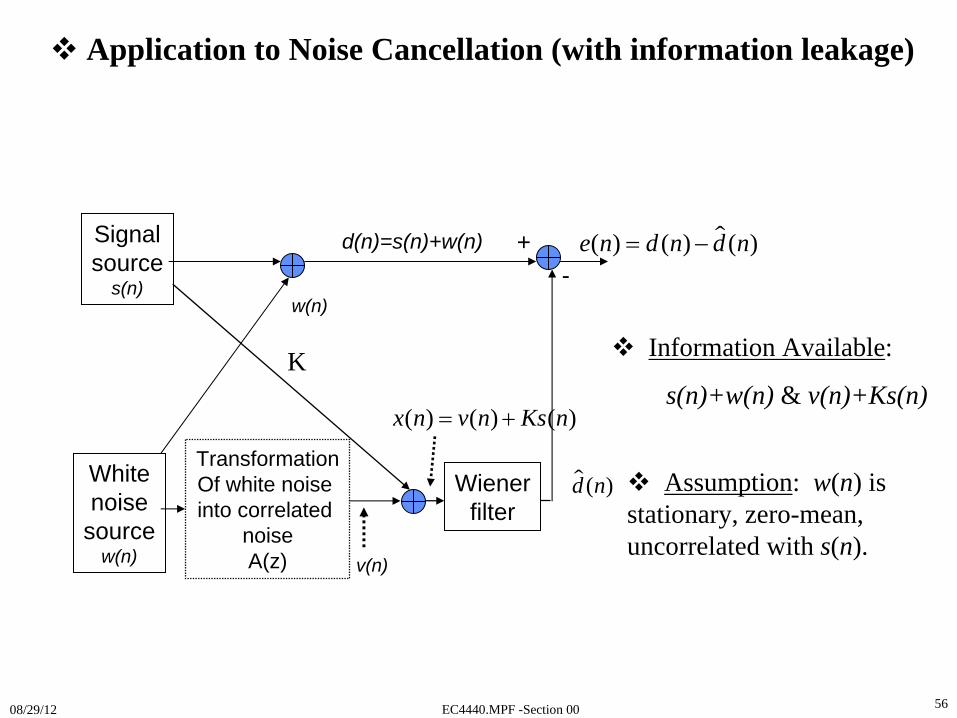
Signalsource

s(n)

Whitenoise

sourcew(n)

Wienerfilter

TransformationOf white noise into correlated

noiseA(z)

w(n)

d(n)=s(n)+w(n) ( ) ( ) ( )e n d n d n= −

v(n)

+

-

( )d n

Application to Noise Cancellation

Goal: Recover s(n) by compensating for the noise distortion while having only access to the related noise distortion signal v(n) (applications in communications, control, etc.)

Information Available:

s(n)+w(n) & v(n)( ) ( )x n v n=

Assumption: w(n) is stationary, zero-mean, uncorrelated with s(n).

EC4440.MPF -Section 0008/29/12 53

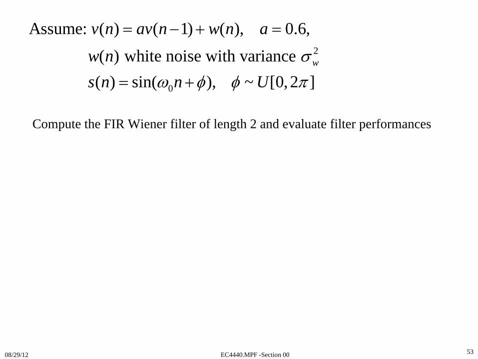
2

0

Assume: ( ) ( 1) ( ), 0.6, ( ) white noise with variance ( ) sin( ), ~ [0,2 ]

w

v n av n w n aw ns n n U

σω φ φ π

= − + =

= +

Compute the FIR Wiener filter of length 2 and evaluate filter performances

EC4440.MPF -Section 0008/29/12 54

EC4440.MPF -Section 0008/29/12 55

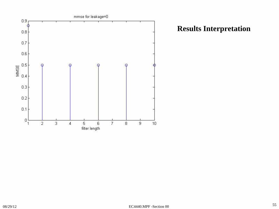
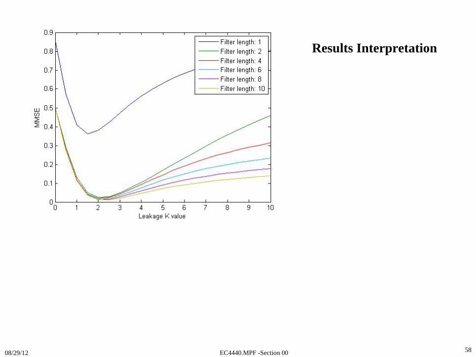
Results Interpretation

EC4440.MPF -Section 0008/29/12 56

Signalsource

s(n)

Whitenoise

sourcew(n)

Wienerfilter

TransformationOf white noise into correlated

noiseA(z)

w(n)

d(n)=s(n)+w(n) ( ) ( ) ( )e n d n d n= −

v(n)

+-

( )d n

Application to Noise Cancellation (with information leakage)

K

( ) ( ) ( )x n v n Ks n= +

Information Available:

s(n)+w(n) & v(n)+Ks(n)

Assumption: w(n) is stationary, zero-mean, uncorrelated with s(n).

EC4440.MPF -Section 0008/29/12 57

EC4440.MPF -Section 0008/29/12 58

Results Interpretation

EC4440.MPF -Section 0008/29/12 59

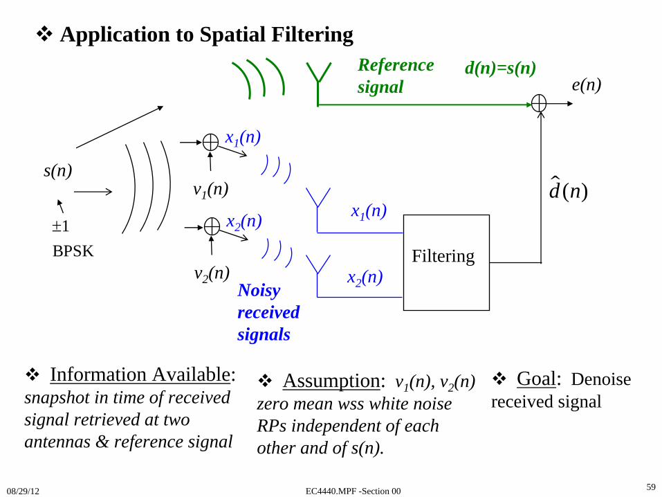
Application to Spatial Filtering

Information Available:snapshot in time of received signal retrieved at two antennas & reference signal

s(n)

1BPSK±

x1 (n)

x2 (n)

d(n)=s(n)e(n)

( )d n

Noisy received signals

x1 (n)

v1 (n)

x2 (n)

v2 (n)

Reference signal

Assumption: v1(n), v2(n) zero mean wss white noise RPs independent of each other and of s(n).

Filtering

Goal: Denoise received signal

EC4440.MPF -Section 0008/29/12 60

Application to Spatial Filtering, cont’

EC4440.MPF -Section 0008/29/12 61

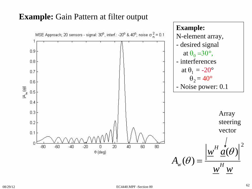
EC4440.MPF -Section 0008/29/12 62

Example:N-element array, - desired signal

at θ0

=30°,- interferences

at θ1

= -20°θ2 = 40°

- Noise power: 0.1

Example: Gain Pattern at filter output

2( )

( )H

w H

w aA

w w

θθ =

Array steering vector

EC4440.MPF -Section 0008/29/12 63

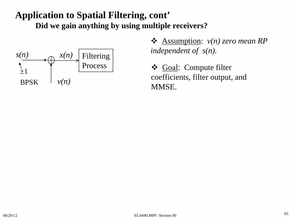
Application to Spatial Filtering, cont’Did we gain anything by using multiple receivers?

FilteringProcess

v(n)

s(n)

1BPSK±

Assumption: v(n) zero mean RP independent of s(n).

Goal: Compute filter coefficients, filter output, and MMSE.

x(n)

EC4440.MPF -Section 0008/29/12 6464

EC4440.MPF -Section 0008/29/12 65

EC4440.MPF -Section 0008/29/12 6666

Appendices

EC4440.MPF -Section 0008/29/12 6767

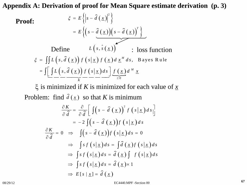
Problem: find so that K is minimum( )d x

Proof:

( )( ),L s s xDefine : loss function

( ){ }( )( ) ( )( ){ }

2

T

E s d x

E s d x s d x

ξ = −

= − −

( )( ) ( ) ( )

( )( ) ( ) ( )0

, , B a ye s R u le

= ,

M

M

K

L s d x f s x f x d x d s

L s d x f s x d s f x d x

ξ

≥

=

⎡ ⎤⎣ ⎦

∫∫∫ ∫

ξ

is minimized if K is minimized for each value of x

( )( ) ( )

( )( ) ( )

2

2

K s d x f s x d sd d

s d x f s x d s

∂ ∂ ⎡ ⎤= −⎢ ⎥⎣ ⎦∂ ∂

= − −

∫

∫( )( ) ( )

( ) ( ) ( )( ) ( ) ( )( ) ( )

( )

0 0

1

[ | ]

K s d x f s x d sd

s f s x d s d x f s x d s

s f s x d s d x f s x d s

s f s x d s d x

E s x d x

∂= ⇒ − =

∂⇒ =

⇒ =

⇒ = ×

⇒ =

∫

∫ ∫∫ ∫∫

Appendix A: Derivation of proof for Mean Square estimate derivation (p. 3)

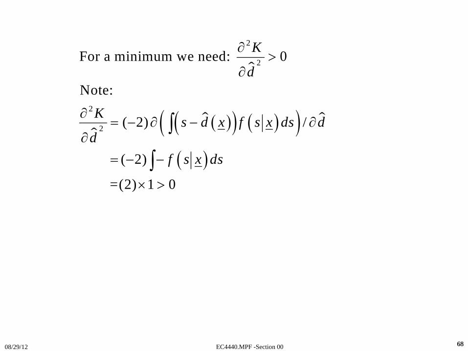
EC4440.MPF -Section 0008/29/12 6868

( )( ) ( )( )( )

2

2

2

2

For a minimum we need: 0

Note:

( 2) /

( 2)

=(2) 1 0

K

d

K s d x f s x ds dd

f s x ds

∂>

∂

∂= − ∂ − ∂

∂= − −

× >

∫

∫

EC4440.MPF -Section 0008/29/12 6969

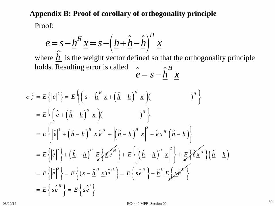
Proof:

where is the weight vector defined so that the orthogonality principle holds. Resulting error is called

( )HHe s h x s h h h x= − = − + −h

He s h x= −

Appendix B: Proof of corollary of orthogonality principle

{ } ( ) ( )

( ) ( )

( ) ( ) ( )

{ } ( ) { } ( ) { }( )

{ } { } { } { }{ } { }

22

22

22

2

*

( )

HH He

H H

H HH H

H HH H

H H H H H

H

E e E s h x h h x

E e h h x

E e h h x e h h x e x h h

E e h h E x e E h h x E e x h h

E e E s h x e E se h E xe

E se E se

σ ⎧ ⎫⎛ ⎞= = − + −⎨⎜ ⎟ ⎬⎝ ⎠⎩ ⎭

⎧ ⎫⎛ ⎞= + −⎨⎜ ⎟ ⎬⎝ ⎠⎩ ⎭

⎧ ⎫= + − + − + −⎨ ⎬

⎩ ⎭⎧ ⎫

= + − + − + −⎨ ⎬⎩ ⎭

= = − = −

= =

EC4440.MPF -Section 0008/29/12 70

References

[1] C.W. Therrien, Discrete Random Signals and Statistical Signal Processing.[2] D. Manolakis, V. Ingle, S. Kogon, Statistical and Adaptive Signal Processing, Artech House, 2005. [3] S. Haykin, Adaptive Filter Theory, Prentice Hall 2002.