0 New Opportunities for Structuring Investment Portfolios Vineer Bhansali, Ph.D. Managing Director, Portfolio Manager, PIMCO Email: [email protected]

1

New Opportunities for Structuring Investment PortfoliosVineer Bhansali, Ph.D.

Managing Director, Portfolio Manager, PIMCO

Email: [email protected]

For Educational Purposes Only

Not for Broad/Printed Distribution

Quant Congress USA, July 8, 2008

This presentation contains the current opinions of the manager and such opinions are subject to change without notice. This presentation has been distributed for informational purposes only and should not be considered as investment advice or a recommendation of any particular security, strategy or investment product. Information contained herein has been obtained from sources believed to be reliable, but not guaranteed. No part of this presentation may be reproduced in any form, or referred to in any other publication, without express written permission of Pacific Investment Management Company LLC. ©2008, PIMCO.

2

Last Year’s Quant Congress (July 12, 2007) – Plenary Session/Vineer Bhansali

Using credit derivatives for hedging

The nature of credit risk in the post-default swap era

The need for hedging arises from market segmentation – what is the structure of the market?

Instruments and their valuation – what are the insurance and hedging aspects and how should we value them? What is the impact of embedded leverage?

Looming uncertainties – settlements, structures, financing frictions, leverage, concentration

Hedge performance measurement

Conclusions: Optimal overlay and hedging vehicles – customization vs. efficiency


3

Back in June of 2007 the 7-100 IG tranche economics looked like this

Tranches are akin to option spreads on indices.

– For instance, a 7-100% tranche on the 7-year Investment-Grade Credit Default Swap Index would cover losses in excess of 7%.

– The CDX and iTraxx indices allow for customization based on client needs and risk preferences.

Expected Loss Table for 10Yr IG8

CDX Index Tranches Expected Loss

0-3% 95.3%

3-7% 55.6%

7-10% 16.6%

7-100% 2.2%

10-15% 7.8%

15-30% 2.5%

30-100% 1.1%

IG8 10 Y 7.1%

Cost Calculation Example: 7-100% Tranche on 10Yr IG8

–For 10 year tranche short at 15.63 bp/year

-Running cost (coupon)/year of spread duration = 2 bp

-Roll-down = 2.67 bp

-Total = 4.67 bp

–To short 1 Billion notional, total lifetime cost is about 12 MM

Risk calculation

–The 10 year index spread duration is 7.45, and the tranche has a delta of 0.53. So each unit of tranche notional provides approximately 7.45*0.53=3.95% return for 100bp spread widening.

Source: PIMCO


4

Same Tranche - Feb. 2008

Tranches are akin to option spreads on indices.

– For instance, a 7-100% tranche on the 7-year Investment-Grade Credit Default Swap Index would cover losses in excess of 7%.

– The CDX and iTraxx indices allow for customization based on client needs and risk preferences.

Expected Loss Table for 10Yr IG9

CDX Index Tranches Expected Loss

0-3% 88.3%

3-7% 54.4%

7-10% 36.2%

7-100% 8.0%

10-15% 23.6%

15-30% 12.1%

30-100% 4.8%

IG8 10 Y 12.2%

Cost Calculation Example: 7-100% Tranche on 10Yr IG8

–For 10 year tranche short at 91 bp/year

-Running cost (coupon)/year of spread duration = 10.1 bp

-Roll-down = 2.2 bp

-Total = 12.3 bp

–To short 1 Billion notional, total lifetime cost is about 67 MM

Risk calculation

–The 10 year index spread duration is 7.35, and the tranche has a delta of 0.77. So each unit of tranche notional provides approximately 7.35*0.77=5.66% return for 100bp spread widening.

Source: PIMCO


5

What’s New this Year?

Macro Tail Risk

– “Tail Risk Management”, Journal of Portfolio Management, Summer 2008.

Momentum

– “Cy-Cular Change”, PIMCO Viewpoints, July 2008. www.pimco.com

6

Tail Risk At The Portfolio Level

Tail risk represents exposure to systematic risk:

– Deleveraging or illiquidity exposure– Puts pressure on ability to fund levered holdings– Correlations rise in absolute value, reducing relevance of basis risk– Risk-Neutral valuation is wrong in this domain

– Tail Risk Hedging cannot be discussed without reference to the whole portfolio

– Factor Approach Captures Systematic Risk

– Principally a handful of factors explain asset movements


7

Four Approaches To Tail Risk Hedging

Move portfolio off the “efficient” frontier, i.e. leave more in “cash”

Purchase high quality insurance securities

– Short term cash and Treasuries natural asset based hedges for tail risk

– But securities may be overpriced for technical reasons

Purchase “Option-like” securities

– Out of the money CDX and ITRAXX indices were “given away” due to high demand

Invest in strategies negatively correlated to tail risk

– ”Trend Following”/Momentum


8

Objective Function

There is no unique tail risk hedge for all seasons and all portfolios.

Tail risk instruments are selected in the portfolio such that stress “beta” is lower than normal beta.

The cost of the insurance, or yield give-up is mathematically equivalent to the certainty equivalent of the difference between the optimal frontier and the truncated portfolio.

To quantify this, scenario shocks of securities – if expected return under scenarios with ex-ante probabilities is higher than the market price, the security qualifies as a good tail-risk security.


9

Analogy - Phase Transitions in Water

Temperature

Pres

sure

Critical Point

Solid

Triple Point

Gas

Liquid

Critical Pressure

Superheated Vapor

Critic

al T

empe

ratu

re

Compressible Liquid

Supercritical Fluid


10

Phase Transitions in Markets

Stable

Markets

Leverage

Ris

k A

vers

ion

Critical Point

Unstable Markets Decreased

Left Tail Risk

Increased Left Tail Risk

Meta-stable

Markets

Critical Risk Aversion


11

Results in Symmetry Breaking and Momentum


12

Consequences

Momentum re. emerges as an investment factor replacing mean-reversion

Monetary Policy has little or no effect

Old benchmarks become irreversibly irrelevant

Fluctuations happen at all scales simultaneously

Arbitrage bounds cease to hold


13

Credit Markets are suffering from run on liquidity – scale invariance

IG on the run spread breakdown (LHS)and average broker CDS (RHS)

from 1/1/08 to 6/9/08

0

10

20

30

40

50

60

70

80

90

100

12/31/07 1/30/08 2/29/08 3/30/08 4/29/08 5/29/08

sp

rea

d (

bp

)

0

50

100

150

200

250

300

350

400

450

idiosyncraticsectorwidesystemic6/9/2008ave broker

Source: PIMCO


14

Negative Basis is persistent and volatile – Breaking of Arbitrage Bounds

-100.00

-80.00

-60.00

-40.00

-20.00

0.00

20.00

40.00

60.00

4/13

/200

5

6/13

/200

5

8/13

/200

5

10/1

3/20

05

12/1

3/20

05

2/13

/200

6

4/13

/200

6

6/13

/200

6

8/13

/200

6

10/1

3/20

06

12/1

3/20

06

2/13

/200

7

4/13

/200

7

6/13

/200

7

8/13

/200

7

10/1

3/20

07

12/1

3/20

07

2/13

/200

8

4/13

/200

8

Source: J.P.MorganFor Educational Purposes Only

15

If momentum is a new risk factor then: Sell the Middle Buy the Tails

Strike effect: People overprice options they can price, but underprice options they cannot price.

Expiration Effect: Due to particular compensation structures sell side is seller of long dated puts

Jump Effect: Markets are discontinuous; models assume continuity


16Source: PIMCO

Momentum Strategies Outperform in Liquidity Events, and have “good” distributional characteristics

-1

-0.75

-0.5

-0.25

0

0.25

0.5

0.75

1

CompositeHedge Fund

ConvertibleArbitrage

DedicatedShort Bias

EmergingMarkets

EquityMarketNeutral

Event Driven Distressed RiskArbitrage

Fixed IncomeArbitrage

Global Macro Long/ShortEquity

ManagedFutures

Multi-Strategy

10yr ended May 08

Jul 07 - May 08

Tech bust (Apr-Nov 00)

LTCM (Aug-Nov 98)

Correlation of Hedge Fund Strategies with VIX


17

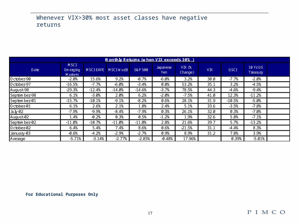
Whenever VIX>30% most asset classes have negative returns

DateMSCI

Emerging Markets

MSCI EAFE MSCI World S&P 500Japanese

YenVIX (% Change)

VIX GSCI 10 Yr US Treasury

October-90 -2.0% 15.6% 9.2% -0.7% -6.0% 3.2% 30.0 -7.7% -2.0%October-97 -16.5% -7.7% -6.0% -3.4% 0.0% 53.2% 35.1 3.2% -4.5%August-98 -29.3% -12.4% -14.0% -14.6% -3.7% 78.5% 44.3 -4.6% -9.4%September-98 6.1% -3.0% 2.0% 6.2% -2.0% -7.5% 41.0 12.3% -11.2%September-01 -15.7% -10.1% -9.1% -8.2% 0.6% 28.1% 31.9 -10.5% -5.0%October-01 6.1% 2.6% 2.1% 1.8% 2.4% 5.1% 33.6 -3.5% -7.8%July-02 -7.9% -9.9% -8.4% -7.9% 0.3% 26.1% 32.0 0.3% -7.0%August-02 1.4% -0.2% 0.3% 0.5% -1.2% 1.9% 32.6 5.8% -7.1%September-02 -11.0% -10.7% -11.0% -11.0% 2.8% 21.6% 39.7 5.7% -13.2%October-02 6.4% 5.4% 7.4% 8.6% 0.6% -21.5% 31.1 -4.4% 8.3%January-03 -0.6% -4.2% -2.9% -2.7% 0.9% 8.9% 31.2 7.8% 3.9%Average -5.71% -3.14% -2.77% -2.85% -0.48% 17.96% 0.39% -5.01%

Monthly Returns (when VIX exceeds 30% )


18

Correlations of Absolute Return Styles shows Trend-Following/Managed Futures is a Lone Diversifier

Source: Khandani & Lo, 2007

Abbreviations:

CA: Convertible ArbitrageDSB: Dedicated Short BiasEM: Emerging MarketsEMN: Equity Market NeutralED: Event DrivenFIA: Fixed Income ArbitrageGM: Global MacroLSEH: Long/Short EquityMF: Managed FuturesEDMS: Event Driven Multi-StrategyDI: DistressedRA: Risk ArbitrageMS: Multi-Strategy

Thick line = > 50% correlation

Thin line = 25 – 50% correlation

No line = < 25% correlation

19

One-Year Correlation of Trend Basic With Other Asset Classes

-0.6

-0.4

-0.2

0

0.2

0.4

0.6

0.8

92 93 94 95 96 97 98 99 00 01 02 03 04 05 06 07 08

LIBOR 1M

MSCI US

Lehman US Agg

VIX

Correlation with other Asset Classes becomes more negative in Crisis Periods

1994 bond and equity bear markets

2000-2002 bear market in equities

1998 Crisis

1999 bond bear market

Trend Strategy is negatively correlated to other asset classes when they perform poorly

On

e-Y

ear

Dai

ly

Cor

rela

tion

Source: PIMCO

20

5-10% Allocation to Momentum Improves Overall Portfolio Sharpe Ratio Calendar Year Returns

-10%

-5%

0%

5%

10%

15%

20%

25%

30%

35%

Optimal Portfolio Sharpe Ratio = 1.2

40/40/20 Sharpe Ratio = 1.0

60/40 Sharpe Ratio = 0.8

MSCI US

LBAGTrends Basic

2007 0.31 0.64 0.062006 0.34 0.60 0.072005 0.32 0.59 0.082004 0.29 0.61 0.102003 0.28 0.59 0.142002 0.24 0.57 0.192001 0.26 0.57 0.172000 0.30 0.50 0.201999 0.32 0.51 0.171998 0.29 0.58 0.131997 0.41 0.42 0.181996 0.48 0.30 0.221995 0.48 0.32 0.211994 0.31 0.58 0.11

Optimal Weights

Optimal stocks/bonds/Momentum = Sharpe Ratio 1.2

40/40/20 stocks/bonds/Momentum = Sharpe Ratio 1.0

60/40 stocks/bonds = Sharpe Ratio 0.8

Source: PIMCO


21

Theory, Practice and Performance of Moving Average Momentum Strategies

22

Are there Anomalies that can be exploited using Priced Based Trading Strategies? Academic Literature now says Yes

Brock, Lakonishok and LeBaron prove that Moving Averages Provide Statistically Significant Profits (1992)

A Study I did in 1993 and 1994, and again in 1999 showed that of all the technical indicators in the “Handbook of Technical Analysis” Moving Averages were the best performing when combining Risk, Return and Simplicity of Execution. Subsequently there has been a lot of work on this in the academic literature.

Fung and Hsieh (2001) show that the trend following strategy is like a long position in a lookback straddle, hence has non-linear factor exposures that cannot be replicated by constant exposures.

The Returns earned on “momentum” strategies can be interpreted as compensations earned for bearing risk during times when inventories are low. “The Fundamentals of Commodity Futures Returns, G. Gorton, F. Hayashi, G Rouwenhorst, 2008.


23

Why do moving average rules work? Some Explanations.

Behavioral:

– Self-Fullfilling: There are enough people following them that they are self-fulfilling.

– Representativeness Bias: Due to reliance on recent data, speculators are prone to behavioral representative biases which lead them to buy asset that are rising and sell those that are falling.

Dynamic Hedging of Options: There is systematic option selling on the tails by hedge funds, and large moves force them to rebalance and rehedge

Virtual Replication of Nonlinear Payoffs: There are trend followers (such as Bridgewater) who replicate the “delta” of a hypothetical option and create momentum (see Fung and Hsieh RFS 2001 paper on trend following replicable using a non-linear option formula equivalent to a lookback straddle).

Policy Inertia: Policy Makers move in small steps, and the market only slowly builds in the extent of the policy changes. (see Anthony Morris paper on the Fed’s creation of momentum in Eurodollar contracts)

Hedging Pressures: There are risk-premia in the market created by the activity of forced hedgers. Hedge sellers sell at lower than fair price, hedge buyers buy at higher than fair price. Speculators and trend followers take the other side to reap benefits as adjustment is slow. (See papers by Spurgin and Scheeneweis).

Inventory Mismatch/Theory of Storage: Momentum is generated by slow adjustment of inventories to demand and supply shocks, transferring commercial hedging premium to trend followers.

Whatever the reasons – the performance and persistence of returns of trend followers warrants closer look, especially in periods of heightened risk.


24

The Math of Trend vs. Mean Reverting Strategies (Source: A. Lo)

Momentum coefficient (+ for momentum, - for mean reversion) and Scaling Rule have to be of same sign to benefit from active mangement. High Volatility periods magnify this effect.

25

It is critical to identify trending vs. Mean-Reverting Markets

26

Testing for Momentum Commodities - Fit to Time Series Models to extract persistence and momentum states.

Dependent Variable: W_1_COMDTYMethod: Least SquaresDate: 03/06/08 Time: 16:56Sample (adjusted): 4/06/1990 1/31/2008Included observations: 4650 after adjustmentsConvergence achieved after 3 iterationsW_1_COMDTY=C(1)+C(2)*(W_1_COMDTY(-1)-C(1))

Variable Coefficient Std. Error t-Statistic Prob.

C(1) 4.25E-06 0.000133 0.032015 0.9745C(2) 0.045517 0.014654 3.106115 0.0019

R-squared 0.002071 Mean dependent var 4.18E-06Adjusted R-squared0.001857 S.D. dependent var 0.008649S.E. of regression0.008641 Akaike info criterion -6.664179Sum squared resid0.347047 Schwarz criterion -6.661407Log likelihood15496.22 Hannan-Quinn criter.-6.663204Durbin-Watson stat1.996628

Positive autocorrelation says this (wheat) is a momentum commodity.

Dependent Variable: SP1_CMDTYMethod: Least SquaresDate: 03/06/08 Time: 16:56Sample (adjusted): 4/06/1990 1/31/2008Included observations: 4650 after adjustmentsConvergence achieved after 3 iterationsSP1_CMDTY=C(1)+C(2)*(SP1_CMDTY(-1)-C(1))

Variable Coefficient Std. Error t-Statistic Prob.

C(1) 0.000118 0.000116 1.011954 0.3116C(2) -0.026129 0.014673 -1.780722 0.075

R-squared 0.000682 Mean dependent var 0.000118Adjusted R-squared0.000467 S.D. dependent var 0.008138S.E. of regression0.008136 Akaike info criterion -6.784666Sum squared resid0.307654 Schwarz criterion -6.781894Log likelihood15776.35 Hannan-Quinn criter. -6.78369Durbin-Watson stat2.000064

Negative-autocorrelation but not significant for SPX.


27

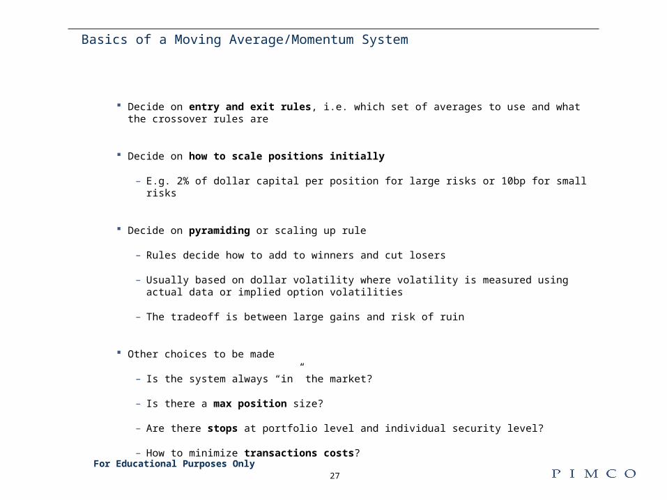
Basics of a Moving Average/Momentum System

Decide on entry and exit rules, i.e. which set of averages to use and what the crossover rules are

Decide on how to scale positions initially

– E.g. 2% of dollar capital per position for large risks or 10bp for small risks

Decide on pyramiding or scaling up rule

– Rules decide how to add to winners and cut losers

– Usually based on dollar volatility where volatility is measured using actual data or implied option volatilities

– The tradeoff is between large gains and risk of ruin

Other choices to be made

– Is the system always “in” the market?

– Is there a max position size?

– Are there stops at portfolio level and individual security level?

– How to minimize transactions costs?


28

0%2%4%6%8%

10%12%14%

-8 -6 -4 -2 0 2 4 6 8 10 12 14

%

Realized DistributionNormal Distribution

-400

-200

0

200

400

600

800

1000

92 93 94 95 96 97 98 99 00 01 02 03 04 05 06 07 08

Trends Basic Returns, 2/1992-5/2008

100

200

300

400

500

600

700

1/27

/199

2

1/27

/199

3

1/27

/199

4

1/27

/199

5

1/27

/199

6

1/27

/199

7

1/27

/199

8

1/27

/199

9

1/27

/200

0

1/27

/200

1

1/27

/200

2

1/27

/200

3

1/27

/200

4

1/27

/200

5

1/27

/200

6

1/27

/200

7

1/27

/200

8

-50%

-45%

-40%

-35%

-30%

-25%

-20%

-15%

-10%

-5%

0%

Base Case (No Costs or Slippage) of a Simple and Stupid System (S-Cubed)

Mean: 84 bp

Std Dev: 368 bp

Skew: 0.61

b p s

Growth of 100

Drawdown

1 yr 3 yr 5 yr 10 yr Since 1992Return (bp) 1527 466 51 541 1000

Std Dev (bp) 1513 1272 1242 1292 1261Sharpe Ratio 1.01 0.37 0.04 0.42 0.79

Monthly Return Distribution

Average Monthly Gain (%) 3.39 T-Stat 3.0

Average Monthly Loss (%) -2.26

Hit Ratio (monthly) 55%

Max Drawdown (since 1991) -19.9%

Calmar Ratio (3Yr) 0.3

Input target Return for 15 years scaled to compare strategies

For Educational Purposes Only Source: PIMCO

29

0%2%4%6%8%

10%12%14%

-6 -4 -2 0 2 4 6 8 10 12 14

%


-1000

-500

0

500

1000

1500

2000

2500

3000

3500

92 93 94 95 96 97 98 99 00 01 02 03 04 05 06 07 08


100

150

200

250

300

350

400

450

500

550

600

1/27

/199

2

1/27

/199

3

1/27

/199

4

1/27

/199

5

1/27

/199

6

1/27

/199

7

1/27

/199

8

1/27

/199

9

1/27

/200

0

1/27

/200

1

1/27

/200

2

1/27

/200

3

1/27

/200

4

1/27

/200

5

1/27

/200

6

1/27

/200

7

1/27

/200

8

-50%

-45%

-40%

-35%

-30%

-25%

-20%

-15%

-10%

-5%

0%

Pyramiding and Profit Stops With No Costs or Slippage: S Cubed + Scaling + Stops

Mean: 84 bp

Std Dev: 309 bp

Skew: 0.74

b p s

Growth of 100

Drawdown









• Go long/short based on momentum signals

• Pyramid up

• Upside volatility stop

For Educational Purposes OnlySource: PIMCO

30

0%

5%

10%

15%

-8 -6 -4 -2 0 2 4 6 8 10121416

%


-1500

-1000

-500

0

500

1000

1500

2000

2500

3000

3500

4000

92 93 94 95 96 97 98 99 00 01 02 03 04 05 06 07 08


100

150

200

250

300

350

400

450

500

550

600

1/27

/199

2

1/27

/199

3

1/27

/199

4

1/27

/199

5

1/27

/199

6

1/27

/199

7

1/27

/199

8

1/27

/199

9

1/27

/200

0

1/27

/200

1

1/27

/200

2

1/27

/200

3

1/27

/200

4

1/27

/200

5

1/27

/200

6

1/27

/200

7

1/27

/200

8

-50%

-45%

-40%

-35%

-30%

-25%

-20%

-15%

-10%

-5%

0%

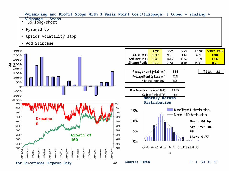
Pyramiding and Profit Stops With 3 Basis Point Cost/Slippage: S Cubed + Scaling + Slippage + Stops

Mean: 84 bp

Std Dev: 387 bp

Skew: 0.77

b p s

Growth of 100

Drawdown


• Go long/short

• Pyramid Up

• Upside volatility stop

• Add Slippage









31

Avg Return vs Avg Position Size

-15%-10%

-5%0%5%

10%15%20%25%

0.0% 0.2% 0.4% 0.6% 0.8% 1.0%

Average Capital (% of Portfolio)A

nn

ual

Ret

urn

Strategy Is Long Gamma (Realized Volatility)

• Trend-following provides cheaper gamma exposure than through options (Kulp, Djupsjöbacka, Estlander, 2005)Average Allocated Capital (VaR)

0.0%

1.0%

2.0%

3.0%

4.0%

5.0%

6.0%

7.0%

8.0%

9.0%

% of P

ortfolio

Natural Gas

Cocoa

Hogs

Live Cattle

Wheat

Soybean

Corn

Heating Oil

Crude Oil

Silver

Gold

Copper

Dollar--Yen

Dollar-Euro

Dollar-Canadian

Dollar-Pound

Eurodollar

5Y Tsy

10Y Tsy

30Y Tsy

S&P 500

R2 = 0.36

Portfolio Risk is Broadly Balanced but puts higher allocation to trending contracts


Source: PIMCO

32

Comparison with Trend-Following Benchmark (MLM or Mount Lucas Management Index)

Mt. Lucas (MLM) Index vs. Trends Basic (Non-Pyramiding)Jan 1991 - May 2008

90

100

110

120

130

140

150

160

Trends Basic (non-pyramiding version)

MLM Index (ex interest)

Mt. Lucas Trends BasicIndex Non-pyramiding

Since inc. rtn 2.4% 1.8%Std dev 5.6% 3.5%Skew (0.17) 0.55 Kurtosis 2.64 0.29 Max drawdown -11.3% -8.6%Sharpe ratio 0.44 0.52


33

… risk-averse investor can capture high returns of 200-400 day moving averages while using stops to reduce volatility

Basic Sharpe Ratio, 1/1992-3/2008

Upside Stop Threshold (times volatility)

Mov

ing

Ave

rage

Len

gth

(d

ays)

Optimal parameter values are {moving average length, stop threshold, pyramid ceiling} = {320, 4.5, 8}

Gradual change in performance with change in parameter values indicates robust system with edge, i.e. earning risk premium

Optimizing Properly Makes System Robust to Volatility


34

Minimum Calmar Ratio of Three Contiguous 5-Year Periods, 4/1993-3/2008

Upside Stop Threshold (times volatility)

Mov

ing

Ave

rage

Len

gth

(d

ays)

Optimal parameter values are {MA length, stop threshold, pyramid ceiling} = {320, 4.5, 8}

Optimizing Properly Makes System Robust to Drawdowns


35

Conclusion

Local models calibrated to a mean-reverting world might still work, BUT ignoring the emergence of momentum and fat-tails is extremely dangerous in the new environment, especially given the low cost of insuring against such outcomes.

This does not require fancy quant modeling, only requires paying attention to leverage, market structure, and deep risk-premium markets.

Documents

0 New Opportunities for Structuring Investment Portfolios Vineer Bhansali, Ph.D. Managing Director, Portfolio Manager, PIMCO Email: [email protected]