A CONCEPTUAL FRAMEWORK FOR THINKING ABOUT ECONOMICDEVELOPMENT AND DEVELOPMENT POLICIES. INFORMAL NOTES

Marco Missaglia and Lucia CornoJanuary 2005

CONTENTS

0. GDP ACCOUNTING1. THE LEWIS MODEL. AN INFORMAL EXPOSITION2. SOME REFINEMENTS OF THE LEWIS FRAMEWORK. POLICY ISSUES3. MIGRATIONS: THE HARRIS-TODARO MODEL 4. LAND REFORMAPPENDIX

0. GDP ACCOUNTING

Measure of Economic Development: GDP per capita (material well-being….)

where : N= Population

L= Labour Force

A, I, S =Agriculture, Industry and Service

where:j

j

LY

= labour productivity in sector J

LL j = proportion of labour force in

sector J

NL = participation Ratio

From (1) we can see the potential sources of the gap in per capita income betweendifferent countries.

a. A difference in the participation ratio. An economy with many children and/orunemployed will have a low ( )NL .

b. A different occupational distribution; since )()( AAII LYLY >> , it is convenient tohave )( LLI as high as possible.

1

c. )( AA LY in the developed countries is roughly 40 times higher than in thedeveloping countries

d. )( II LY in the developed countries is roughly 10 times higher than in thedeveloping countries.

Thus, there is considerable scope for increasing labour productivity in agriculture indeveloping countries. However, statistically speaking, reason b. is by far the mostimportant in explaining the gap (income gap) between developed and developing countries,which provides the central justification for an industrialization–led development strategy: theproblem of development may be seen as the problem of moving people from agriculture toindustry, to increase the relative size of the industrial sector. How can this objective be achieved? We need a broad conceptual framework to thinkabout this transition, and this conceptual framework lies at the core of developmenteconomics.

1. THE LEWIS MODEL (1954). AN INFORMAL EXPOSITION

If development is structural change (Agriculture→ Industry→ Service), the main roles ofagriculture are:

1. Supplier of labour to industry (people move)2. Supplier of a surplus of food. If international trade is not an option (and it is

not to the extent that countries want to achieve self sufficiency in this isextremely important field), then a non-agricultural sector can develop only ifagricultural produces more food than its producers need for their ownconsumption: this is the agricultural surplus.

There is also a third role played by the agricultural sector:

3. Source of demand for industrial products, given the relevant size of agriculturein a developing economy, Lewis is mainly concentrated on roles (1) and (2).

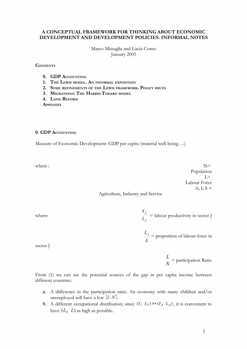
Lewis model has in mind a dual economy

Traditional Sector Modern Sector

Basically, but Basically, butnot only not only rural/agricultural urban/industrial

2

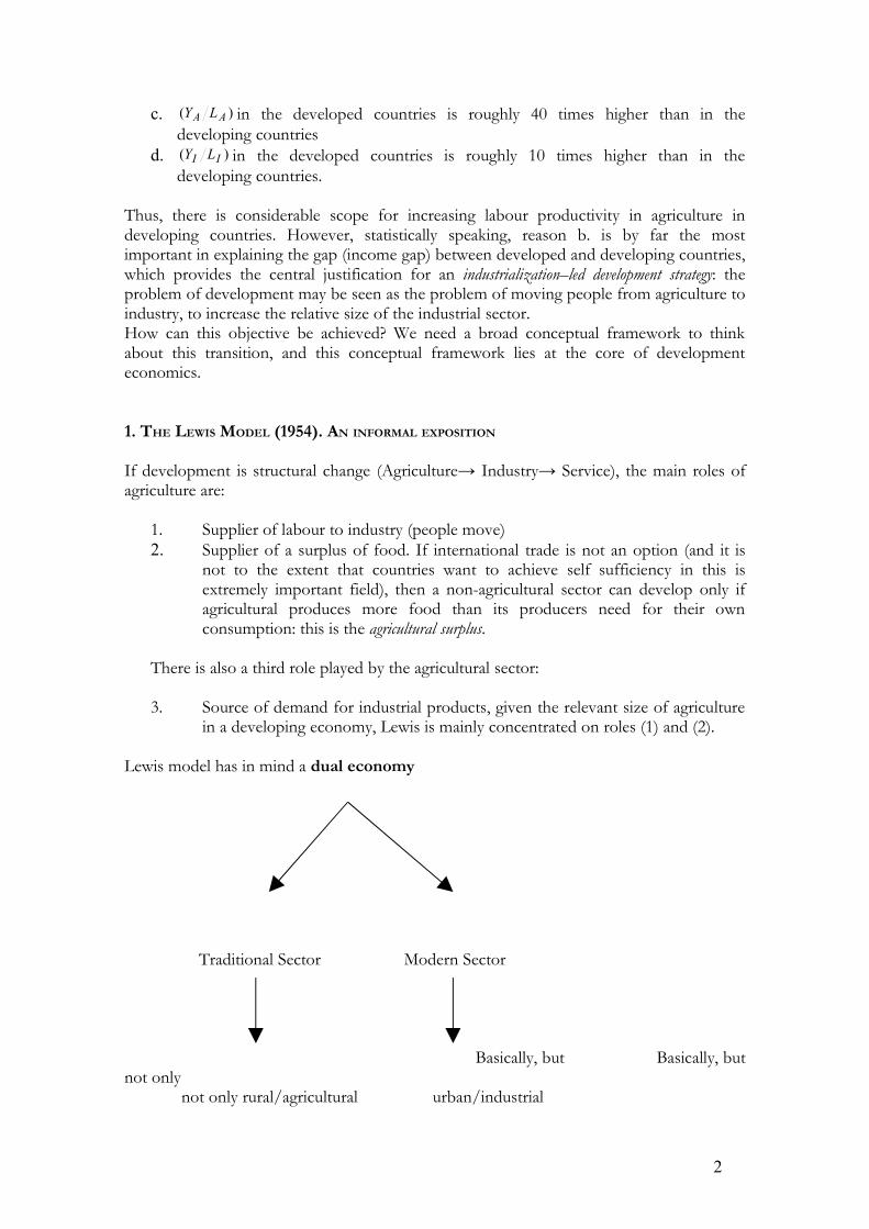
What is,economically speaking, the main feature of the traditional sector?It is the existence of surplus labour or disguised unemployment. What does it mean? Be La theamount of labour employed in agriculture; the production function with surplus labour is:

Figure 1: the production function in agriculture

In the background of this production function: a very limited quantity of capital (we arebasically in a non-capitalistic, pre-modern sector) and a fixed amount of land (from whichdiminishing returns to labour).For any LA ≥ B, the marginal product of labour in agriculture in nil.

Then, if you reduce labour from A to B ≡ LABOUR SURPLUStotal output is unchanged

For a capitalist, the profit maximizing rule is

Real wage = Marginal product of Labour ( LMP )

But what happens in a family farm with labour surplus, where LMP = 0 ?People are not paid their marginal product, because the objective of the family farm is notprofit maximization, but to guarantee an income to each of its members (an egalitarian, orpre-capitalistic rule, as opposed to a capitalistic rule). People are paid their average product w (thishappens in the informal sector as well, in the cities. A cub driver might share his drivingwith a friend)

3

La

Y

B A

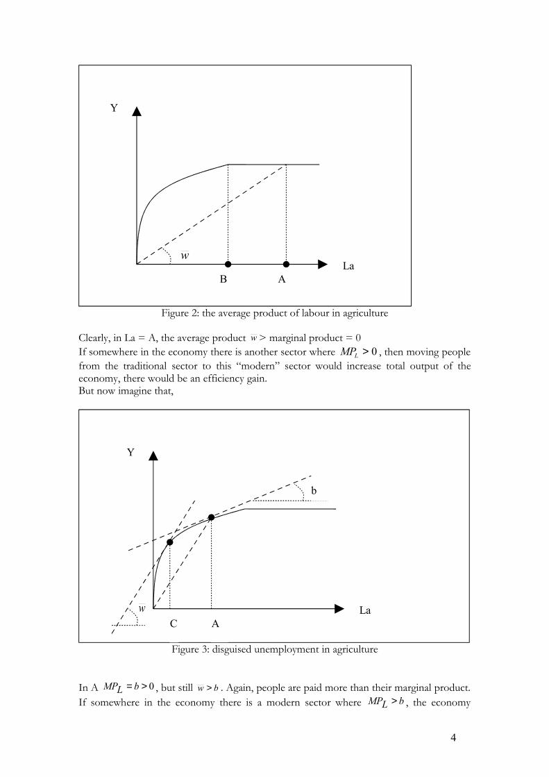
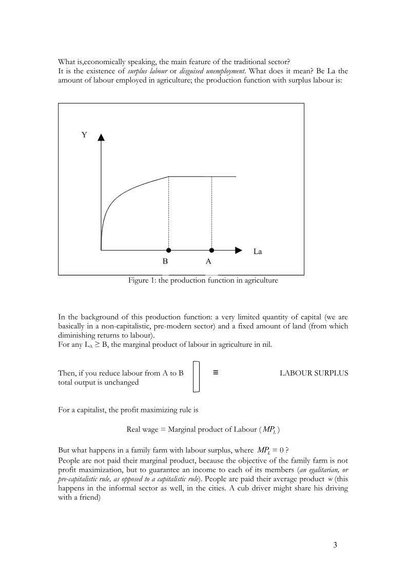
Figure 2: the average product of labour in agriculture

Clearly, in La = A, the average product w > marginal product = 0If somewhere in the economy there is another sector where 0>LMP , then moving peoplefrom the traditional sector to this “modern” sector would increase total output of theeconomy, there would be an efficiency gain.But now imagine that,

Figure 3: disguised unemployment in agriculture

In A 0>= bLMP , but still bw > . Again, people are paid more than their marginal product.If somewhere in the economy there is a modern sector where bLMP > , the economy

4

La

Y

C A

b

w

La

Y

B A

w

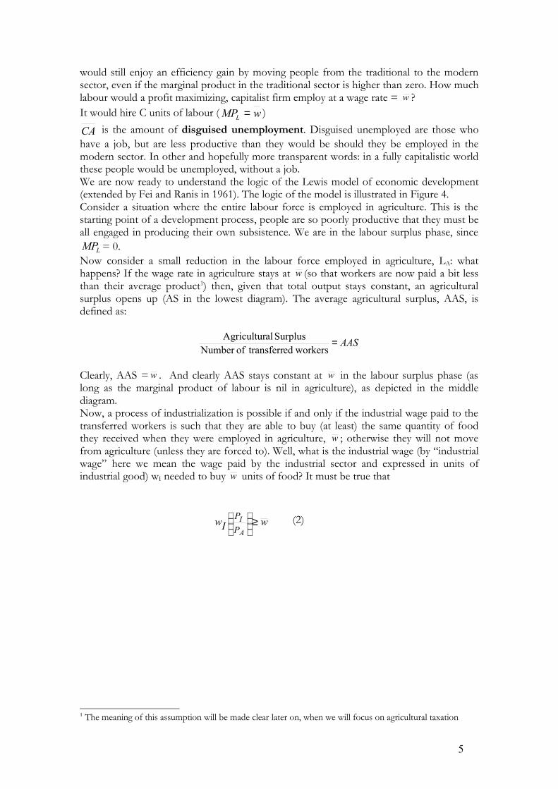
would still enjoy an efficiency gain by moving people from the traditional to the modernsector, even if the marginal product in the traditional sector is higher than zero. How muchlabour would a profit maximizing, capitalist firm employ at a wage rate = w ?It would hire C units of labour ( wMPL = )

CA is the amount of disguised unemployment. Disguised unemployed are those whohave a job, but are less productive than they would be should they be employed in themodern sector. In other and hopefully more transparent words: in a fully capitalistic worldthese people would be unemployed, without a job.We are now ready to understand the logic of the Lewis model of economic development(extended by Fei and Ranis in 1961). The logic of the model is illustrated in Figure 4.Consider a situation where the entire labour force is employed in agriculture. This is thestarting point of a development process, people are so poorly productive that they must beall engaged in producing their own subsistence. We are in the labour surplus phase, since

LMP = 0.Now consider a small reduction in the labour force employed in agriculture, LA: whathappens? If the wage rate in agriculture stays at w (so that workers are now paid a bit lessthan their average product1) then, given that total output stays constant, an agriculturalsurplus opens up (AS in the lowest diagram). The average agricultural surplus, AAS, isdefined as:

AAS= workersed transferrofNumber

Surplus alAgricultur

Clearly, AAS =w . And clearly AAS stays constant at w in the labour surplus phase (aslong as the marginal product of labour is nil in agriculture), as depicted in the middlediagram.Now, a process of industrialization is possible if and only if the industrial wage paid to thetransferred workers is such that they are able to buy (at least) the same quantity of foodthey received when they were employed in agriculture, w ; otherwise they will not movefrom agriculture (unless they are forced to). Well, what is the industrial wage (by “industrialwage” here we mean the wage paid by the industrial sector and expressed in units ofindustrial good) wI needed to buy w units of food? It must be true that

wIwA

IPP ≥

(2)

1 The meaning of this assumption will be made clear later on, when we will focus on agricultural taxation

5

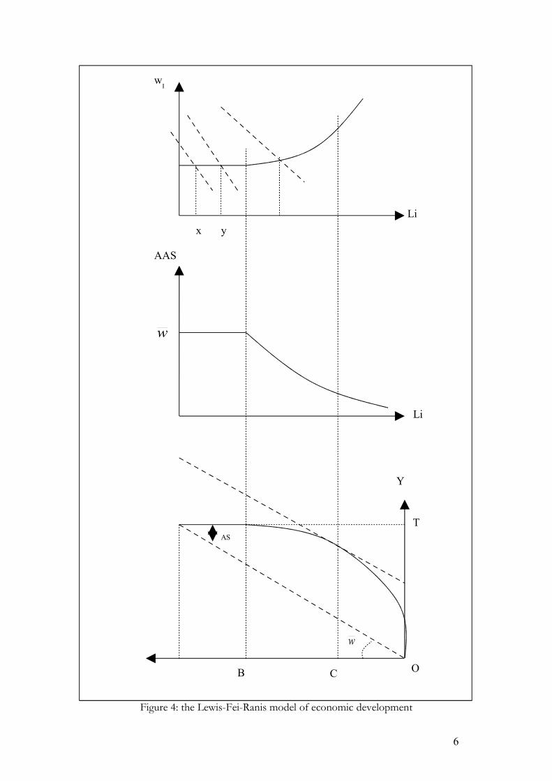
Figure 4: the Lewis-Fei-Ranis model of economic development

6

LaA B

T

Y

AAS

Li

Li

wI

w

w

x y

O

AS

C

However, industrialists want to make as much money as they can, and therefore (2) willhold as a strict equality (they do not want to pay more than is strictly needed to attractpeople from the rural/informal sector):2

pwwIwI

APP ==

(3)

From (3) we can see that, for any given level of the terms of trade IA PP (henceforthsimply p for brevity), the industrial wage is constant as far as the agricultural wage w staysconstant as well, i.e. in the labour surplus phase. This is shown in the upper diagram.Let’s now analyse the disguised unemployment phase (BC), i.e. the phase where inagriculture 0>LMP but, assuming that the agricultural wage keeps staying constant (seefootnote 1), LMPw > ? The average agricultural surplus begins to decline (since total outputgoes down); this can be seen by inspection of the lowest diagram and is shown in themiddle one. One can therefore guess that, since less agricultural output is marketed (eachworker that moves away from agriculture has to buy food on the market, but on averageless food is available), food (agriculture) prices start to rise. But look at equation (3): the increase in p will push the industrial wage (w*) up, in order tomake industrial workers able to buy w units of food and hence give them the appropriateincentive to move to industry. However, at a closer inspection, we can see that even if theindustrial workers are getting more than w*, it is simply impossible for them to buy wunits of food, because there is not enough to go around. To see why, just consider that byassumption people employed in agriculture are getting w ; if each industrial worker boughtw as well, total agriculture production should be equal to OT, which is not the case. Itfollows that, at this stage, industrial workers will have to consume a mix of industrial andagricultural products. Under these conditions, will the potential “migrants” accept to moveto industry? Clearly, they will if and only ifw is not too close to the subsistence level (if itwere, it could not be reduced!). This is a very important result, it says that agriculture mustbe sufficiently productive to favour an industrialisation process. In any case, potential“migrants” will only accept an industrial wage higher than w*: this is the reason why in theupper diagram the industrial wage becomes an increasing function at the beginning of thedisguised-unemployment phase.When the transfer of labour reaches point C the disguised unemployment phase comes toan end. In theCO region wMPL > : agriculture is likely to become a fully capitalistic sectorwhere wages are set according to the profit-maximisation rule (real wage = marginalproduct of labour). It follows that as labour moves from agriculture to industry, agriculturalwage goes up (in other words, the wage bill in agriculture falls more slowly than before aslabour moves from agriculture to industry) and the industrial wage (in the topmost panel)must increase even faster since it must not only compensate for higher terms of trade (p),but also for higher incomes in the agricultural sector.We are now ready to read properly the topmost panel where we have drawn a family oflabour demand curves. For easiness of exposition, let us redraw that diagram:

2 For more realistic cases, a mark-up for higher costs of living in the urban sector or a lager degree ofunionization in the industrial sector as well as some discount factor for the uncertainty of getting a job in thecity are all factors that could be added to this simple model. However, they would not change the mainconclusions in any relevant aspect.

7

Figure 5: The process of industrialization

Initially, the amount of industrial labour is x. Realised profits are equal to Πx3 and Lewis

assumes they are automatically invested back into the industrial activities (there is not aninvestment function in the Lewis – Fei – Ranis model). With more capital, labour demand(the marginal product of labour) shifts up. The new level of industrial employment is y.Note that in this labour surplus phase new industrial labour is forthcoming at the fixed realwage w*. Despite the fact that the marginal productivity of labour in the industrial sector isgoing up, the real wage earned by each worker stays constant. In the labour surplus phasethe fruits of industrial expansion are not equally distributed: labour is becoming more andmore productive but this only translates into higher profits (Πy + Πx > Πx) So, one of theimplications of Lewis’ view of economic development is that income distribution (at leastfunctional income distribution) worsens in the early phases of industrialisation (somethingreflected in the well known Kuznets curve). This important issue of the link betweenindustrialisation and income distribution will be further investigated below with the help ofa formal model developed by Bourgignon (1990). But it is in any case worth stressing thatthis unpleasant distributive result is seen by Lewis as an element that helps the economygrow and industrialise faster: industrialisation comes from capital accumulation and capitalaccumulation comes from profits (the propensity to save out of profits is higher than thepropensity to save out of wages). And, do not forget our initial remarks, per capita incomegrowth is facilitated by industrialisation.

3 By definition of marginal product, total industrial production is equal to the area OXYx; the industrial wagebill equals the rectangle (OX)w* and what is left, the triangle Πx, goes to profit earners.

8

xπ yπ

x y

Iw

*w

O

Yx

IL

As is should be clear by our diagrams, once the labour surplus phase is exhausted,industrial employment can only rise at the price of an increasing wage and, not surprisingly,the very pace of industrialisation is likely to slow down. To summarise, the basic ideas of economic development ( = industrialization) behind theLewis – Fei – Ranis model are:

a. the engine of growth is capital accumulation (no problem of demand, saving areautomatically reinvested. Keynes’ preoccupation about the level of effectivedemand was considered something relevant for rich economies only).

b. As development proceeds, there is a process of rural – urban migration andurbanisation.

c. As development proceeds, the terms of trade p increase. Food prices risebecause a smaller and smaller number of farmers must support an increasingnumber of industrial workers.

Briefly: “development” is driven by capital accumulation but limited by the ability of theeconomy to produce a surplus of food (the lower the surplus → the higher p → the higherthe industrial wage → the weaker the incentive to invest in the industrial sector).

The policy implications of such a view are very much controversial and hotly debated.Consider for instance the role of agriculture. Even if we accept the residual role given toagriculture in the Lewis framework (agriculture as a source of cheap labour and supplier ofa food surplus), the question is: how these potentialities of agriculture are best exploited?By taxing agriculture, which would expand industrial labour supply (it is easier to convincepeople to move away from agriculture when agriculture is taxed), or by subsidising agriculture(for instance helping farmers buy relevant inputs like water, fertilisers, etc.), which wouldexpand agricultural production and the available surplus of food? And what happens whenagriculture does not coincide with food production alone, but it includes the production ofnon-food items as well? Again: provided that technical progress in agriculture is good forgrowth and industrialisation (since it raises the surplus of food), are we sure that in a pooreconomy there are the appropriate incentives to introduce better agricultural techniques ofproduction? In this respect, what is the role of land reforms and land redistribution? How isthe Lewis picture modified by the introduction of international trade and globalisation? Isthe kind of development process depicted in the model necessarily associated with aworsening income distribution (growth for whom?) or some more pleasant outcome maybe envisaged? In the following sections we will complicate a bit the Lewis framework inorder to address some (not all) of these policy issues.

2. SOME REFINEMENTS OF THE LEWIS FRAMEWORK. POLICY ISSUES.

Technical progress in agriculture and agricultural taxation

According to the "accumulationist" view of Lewis, the process of industrialization is clearlyhelped by maintaining for a sufficiently long period of time a low level of the industrialwage. The longer the industrial wage stays at w*, the quicker the industrialization processwill be, since more profits will be available for (automatic) re-investment. But look atequation (3). It is quite clear that the level of the industrial wage is ultimately determined bythe wage prevailing in agriculture and by the agricultural terms of trade, p. It follows thatthe policy question is: how can these two variables be kept at a low level so as to ease theindustrialization process? In principle, there are several possibilities, but each of thementails serious difficulties.

9

• AGRICULTURAL TAXATION. As people move from the rural to the manufacturing sectorand the economy is in the labor surplus phase, the average product of labor inagriculture goes up. It follows that if farmers are paid their average product, theagricultural wage should go up, which is bad for industrialization. One way of escapingthis trap is to tax agriculture: the net payment accruing to the farmer stays at w (seefootnote 1) because the excess of the average product over w goes to the government.However, by discouraging agricultural production, such a measure could provoke a(faster) rise in the agricultural terms of trade, which in turn could slow theindustrialization process. It has often been argued that Africa was a typical example ofexcessive taxation on agriculture, and this is the reason why several African countriesimplemented market-oriented reforms over the last ten years. The case of Africa, forobvious reasons, deserves a closer scrutiny. We should first try to understand whetheragricultural has suffered from an excess of taxation. Then we should have a look at thebehaviour of the agricultural terms of trade over the last decades and finally try to studythe relation between agricultural production and real producer prices. Of course, thesepoints are closely related to each other, but let us investigate them separately.Is it true that Africa agriculture used to be too heavily taxed? To answer this question itis important to distinguish among three kinds of agricultural products: exportable(cocoa, cotton, coffee, tobacco, etc.), importable (food crops such as cereals) and non-tradable (cassava, plantain, millet, sorghum, white maize and other typically “African”food staples, which are not consumed outside Africa). As to the exportable, a way ofaddressing the question of their taxation is to look at the margin between export prices(i.e. the world price of the crop expressed in dollars multiplied by the nominalexchange rate) and prices actually received by farmers. Of course we are discussing thecase when producers and exporters are different entities (and not when producersexport directly, as in the case of plantation and agribusiness based on transnationalcorporations). In several African countries, from the days of the independence to theearly 1990s, public marketing boardswere the principal exporting entity. The differencebetween the price earned in the international markets by a public marketing board andthe price paid by the marketing board to the farmer is to be considered a “tax” paid bythe latter to the government (in light of the public nature of the marketing board). Sure,such a difference is a crude approximation of the degree of taxation since no allowanceis made for marketing and transportation costs. As a consequence, we have to take themargin as an overstatement of the true degree of taxation. Moreover, it must bestressed that the degree of taxation is linked to the exchange rate. A devaluation (i.e. ahigher nominal exchange rate, you need more pesos to buy a dollar) would raise thedomestic currency price received by the exporters (by the marketing board). If pricespaid to farmers remain unchanged (or are raised by less than the rate of currencydevaluation), the tax rate will rise4. With all this caveats in mind, the evidence presentedby UNCTAD (TDR 1998, pp. 156-159) does not support the widespread view thatAfrican producers have always been more heavily taxed than those in other developingcountries. Of the five export crops studied (coffe, cocoa, tea, cotton, tobacco) withreference to the period 1970-1994, it is only for cocoa and tobacco that the marginbetween border and producer prices was significantly higher in Africa than in the othermajor exporters. It must be added that this kind of exportables are not consumed bythe farmers as “food” and therefore, even if they were excessively taxed (which is nottrue, as we have just seen), this would not contribute to slow the migration of peoplefrom the agricultural to the manufacturing sector. On the contrary, it could be argued

4 However, when devaluations lead to a widening of the margin but the price paid to the export producersgoes up at least a bit, this tends to raise real producers prices of export crops vis-à-vis nontradables, thusproviding incentives for export.

10

along the same lines followed in the illustration of the Lewis model that this could evenaccelerate the industrialisation process. To see why, just go back to equation (3) andread it from the point of view of a producer of an exportable good like cocoa or coffee.The terms of trade p must be interpreted as the ratio between the price of food (notcoffee or cocoa) and the price of the manufactured good; Iw is the wage paid by theindustrial sector expressed in units of industrial good and, finally, w is the real wageearned by the coffe or cocoa producer expressed in units of food. w can thus bethought of as the net nominal earning of the coffee or cocoa producer divided by theprice of food. Well, even admitting (in a counterfactual exercice) that the taxation onthe exportable good is somehow excessive, this should decrease w and thereforestimulate the transfer of people to the urban areas. Fresh workforce available for theindustrialisation process. Still, the general belief that these exportables were too heavilytaxed lead at the end of the 1980s to a major reform process. In most African countriesthe marketing boards were simply abolished and devaluations were applied to severalcurrencies. The idea was to eliminate the tax paid by the exportable producers byeliminating the tax collector (the marketing board) and to provide further incentives tothe exporters through a currency devaluation. Well, it may be surprising to see thatfrom the beginning of the reform process until mid-90s the ratio between producer andexport prices has declined for all the five products considered except coffee. Why is itthat the elimination of the tax collector actually lead to a raise in the tax paid by theproducers? Because the reform process was based on ideology rather than governed bypragmatism. Indeed, eliminating a marketing board does not imply that a producer(and, let us repeat, we are not talking about transnational companies and plantations)suddenly becomes able to sell to the international market. She still needs a trader, and ifa public trader (a marketing board) is not there, a private one will enter into the picture.No doubt, this private trader will try to maximise his profits and, when faced with acurrency devaluation, what will he do? He will increase the price paid to the producerby less than the devaluation rate and therefore there should not be any surprise to seethat the reform process was actually accompanied by an increase in the degree oftaxation of the major export crops5. What about the importable goods? Here we are talking about goods such as rice, wheatand maize. A local producer can be said to be taxed when the net price she gets islower than the price paid (in domestic currency) to import the same good. On thecontrary, a local producer is said to be subsidized when the net price she receives ishigher than the domestic currency import cost6. Well, from 1970 to 1994 the producerprice for this importable good had been systematically higher than the unit import cost,which indicates a positive rate of subsidization (UNCTAD, TDR 1998, Chart 16). Inprinciple, this should stimulate the production of these food items, lower the terms oftrade p (look again at equation 3) and thus favour the industrialisation process for anygiven level of the real (food) wage earned by farmers.

5 It must be stressed that a further drawback of this reform was the disappearance of the public moneyformerly in the pockets of the marketing board. Even when it is heavily corrupted, you can ask a state to buildsome roads or develop some utilities. But if the “tax” collector is a private trader, you can’t ask anything.6 A numerical example may be useful. Imagine that the world price of a unit (a kilo, a ton, a trunk, whateveryou like) of rice is 200 US$. In the country we are considering the exchange rate is 10 pesos per dollar and atariff of 15% is applied to the import of rice. Thus the overall price paid by the locals to buy a unit of riceproduced abroad is 200x10x1.15 = 2,300 pesos. If some kind of competition is at work (and usually it is), theprice applied by local producers to sell their own rice will be exactly the same, 2,300 pesos. In this case, localproducers are said to be (implicitly) subsidized since the price they get (2,300) is higher than the import costnet of tariff (2,000). A tariff is not the only way of protecting a local farmer. Another possibiity is to subsidizethe purchase os some relevant input (water, fertilizers, etc.). In this case the consumers will pay less than thedomestic currency world price to buy rice, but the net price (inclusive of the subsidy) received by the localproducers will be higher than the domestic currency world price.

11

As to the non-tradables, lack of data (to our knowledge) makes it impossible to saysomething relevant, but the former analysis should have made clear that it is hard to saythat agriculture in Africa has suffered from an excess of taxation and this has slowed oreven blocked the industrialisation process. All the more so after the reforms and thedismantling of the marketing boards.At this point, a question naturally arises: what are the likely reasons of the missingAfrican agricultural development? There is no doubt that a serious industrialisationprocess cannot even start without a significant growth of agricultural productivity, butthe foregoing analysis should have convinced the reader that the main problem doesnot lie in perverse (insufficient) price incentives. The main problem for Africanagriculture is the weak response to price incentives: even when prices are high or go up,this is not enough to stimulate more production. There are a host of institutional andstructural factors that may explain this feature. Let us see the most important. In theshort run, aggregate supply response to price incentives can occur through two basicprocesses: either idle land is brought into use or more variable inputs (labour,fertilizers, etc.) are put at work on a given unit of land. In the long run, aggregatesupply response is mainly determined by investment and productivity growth. Well,even when there are community land resources available (which is not always the case),poorer farmers simply cannot farm extra land because they cannot mobilize thenecessary complementary inputs. On top of this, high levels of poverty means thatfarmers cannot afford to keep either their labour or land idle even at very unattractiveprices. As to the intensification of the agricultural process, i.e. the use of more variableinputs on a given unit of land, one of the rason why after the reform process the supplyresponse to higher output prices7 was weak lies in the behaviour of the input prices.Indeed, together with the abolition of the marketing boards, African farmers had toface the removal of the subsidies to buy such items like fertilizers. There is somethingmore: even in the presence of an appropriate incentive for the farmers to put morevariable inputs at work, it must be recognized that buying these extra inputs requiressome credit. Well, “the marketing boards had offered an institutional response to theproblem of missing private credit markets. As they had a legal monopsony overmarketed output, they could provide seasonal inputs on credit against the potentialcrop as collateral......With privatization, this system of seasonal credit has brokendown” (UNCTAD, TDR 1998, p.169). Sure, the role once played by the marketingboards is now played by private traders, but obviously the latter, being moved by thesacred principle of profit maximization, apply tougher conditions to the farmers8. And,last but not least, the money earned by a private trader cannot be used (unless you areable to impose a tax) to finance the provision of public goods.The issue of pubblic goods (or in any case private goods whose production entailsstrong positive externalities) is strictly connected to the long run response ofagricultural output to price incentives. There cannot be any significantly positiveresponse unless better infrastructure is available, especially transport9. Again: togetherwith the dismantling of the marketing boards and the removal of the subsidies oninputs, “reforms” usually asked for a cut of public expenditures...

7 Remember that the basic idea behind the dismantling of the marketing boards was to increase the pricedirectly received by the producer.8 See the Appendix for a formal analysis of the relation between a farmer-borrower and a private trader-lender.9 The rural transport bottleneck is so important because it prompts two negative effects. First, it reduces thereal return to a given investment (let us say that the cost of bringing to the market the goods produced thanksto the investment goes up) and, second, it is a source of product market imperfections (if the transportnetwork is underdeveloped, a small farmer must sell to a trader and this lowers her market power)

12

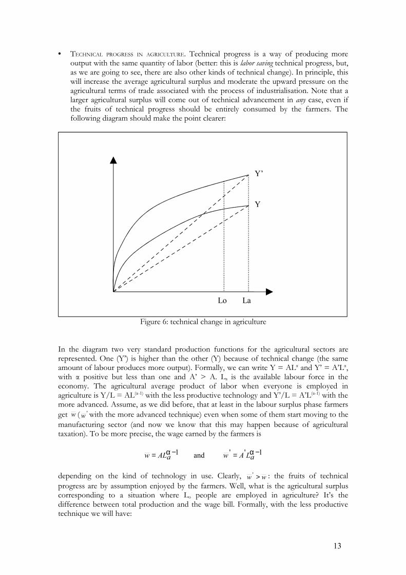
• TECHNICAL PROGRESS IN AGRICULTURE. Technical progress is a way of producing moreoutput with the same quantity of labor (better: this is labor saving technical progress, but,as we are going to see, there are also other kinds of technical change). In principle, thiswill increase the average agricultural surplus and moderate the upward pressure on theagricultural terms of trade associated with the process of industrialisation. Note that alarger agricultural surplus will come out of technical advancement in any case, even ifthe fruits of technical progress should be entirely consumed by the farmers. Thefollowing diagram should make the point clearer:

Figure 6: technical change in agriculture

In the diagram two very standard production functions for the agricultural sectors arerepresented. One (Y’) is higher than the other (Y) because of technical change (the sameamount of labour produces more output). Formally, we can write Y = ALα and Y’ = A’Lα,with α positive but less than one and A’ > A. La is the available labour force in theeconomy. The agricultural average product of labor when everyone is employed inagriculture is Y/L = AL(α-1) with the less productive technology and Y’/L = A’L(α-1) with themore advanced. Assume, as we did before, that at least in the labour surplus phase farmersget w ( 'w with the more advanced technique) even when some of them start moving to themanufacturing sector (and now we know that this may happen because of agriculturaltaxation). To be more precise, the wage earned by the farmers is

1'' and 1 −=−= αα aLAwaALw

depending on the kind of technology in use. Clearly, ww >' : the fruits of technicalprogress are by assumption enjoyed by the farmers. Well, what is the agricultural surpluscorresponding to a situation where Lo people are employed in agriculture? It’s thedifference between total production and the wage bill. Formally, with the less productivetechnique we will have:

LaLo

Y

Y’

13

−−=−−= 011 LaLoLAoLaALoALAS αααα ,

and with the more advanced technique

−−=−−= 01'1''' LaLoLAoLaLAoLAAS αααα .

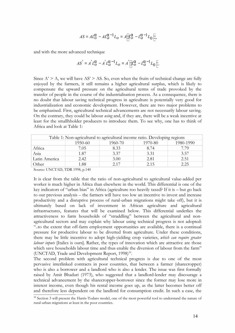
Since A’ > A, we will have AS’ > AS. So, even when the fruits of technical change are fullyenjoyed by the farmers, it still remains a higher agricultural surplus, which is likely tocompensate the upward pressure on the agricultural terms of trade provoked by thetransfer of people in the course of the industrialisation process. As a consequence, there isno doubt that labour saving technical progress in agriculture is potentially very good forindustrialization and economic development. However, there are two major problems tobe emphasised. First, agricultural technical advancements are not necessarily labour saving.On the contrary, they could be labour using and, if they are, there will be a weak incentive atleast for the smallhholder producers to introduce them. To see why, one has to think ofAfrica and look at Table 1:

Table 1: Non-agricultural to agricultural income ratio. Developing regions1950-60 1960-70 1970-80 1980-1990

Africa 7.05 8.33 8.74 7.79Asia 1.87 3.37 3.31 3.57Latin America 2.42 3.00 2.81 2.51Other 1.88 2.17 2.15 2.25Source: UNCTAD, TDR 1998, p.140

It is clear from the table that the ratio of non-agricultural to agricultural value-added perworker is much higher in Africa than elsewhere in the world. This differential is one of thekey indicators of “urban bias” in Africa (agriculture too heavily taxed? If it is – but go backto our previous analysis – the farmers will have too low an incentive to invest and increaseproductivity and a disruptive process of rural-urban migrations might take off), but it isultimately based on lack of investment in African agriculture and agriculturalinfrastructures, features that will be examined below. This differential underlies theattractiveness to farm households of “straddling” between the agricultural and non-agricultural sectors and may explain why labour using technical progress is not adopted:“..to the extent that off-farm employment opportunities are available, there is a continualpressure for productive labour to be diverted from agriculture. Under these conditions,there may be little incentive to adopt high-yielding crop varieties, which can require greaterlabour inputs [Italics is ours]. Rather, the types of innovation which are attractive are thosewhich save households labour time and thus enable the diversion of labour from the farm”(UNCTAD, Trade and Development Report, 1998)10. The second problem with agricultural technical progress is due to one of the mostpervasive interlinked contracts in poor countries, that between a farmer (sharecropper)who is also a borrower and a landlord who is also a lender. The issue was first formallyraised by Amit Bhaduri (1973), who suggested that a landlord-lender may discourage atechnical advancement by the sharecropper-borrower since the former may lose more ininterest income, even though his rental income goes up, as the latter becomes better offand therefore less dependent on the landlord for consumption credit. In such a case, the10 Section 3 will present the Harris-Todaro model, one of the most powerful tool to understand the nature ofrural-urban migrations at least in the poor countries.

14

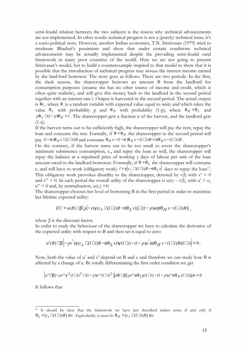
semi-feudal relation between the two subjects is the reason why technical advancementsare not implemented. In other words: technical progress is not a (purely) technical issue; it’sa socio-political story. However, another Indian economist, T.N. Srinivasan (1979) tried tomoderate Bhaduri’s pessimism and show that under certain conditions technicaladvancements may be actually implemented despite the prevailing semi-feudal ruralframework in many poor countries of the world. Here we are not going to presentSrinivasan’s model, but to build a counterexample inspired to that model to show that it ispossible that the introduction of technical progress may increase the interest income earnedby the land-lord borrower. The story goes as follows. There are two periods. In the first,the slack season, the sharecropper borrows an amount B from the landlord forconsumption purposes (assume she has no other source of income and credit, which isoften quite realistic), and will give this money back to the landlord in the second periodtogether with an interest rate i. Output is harvested in the second period. The actual outputis xθ , where θ is a random variable with expected value equal to unity and which takes thevalue Lθ with probability p and Hθ with probability (1-p), where LH θθ > and

1)1( =−+ HL pp θθ . The sharecropper gets a fraction α of the harvest, and the landlord gets(1-α).If the harvest turns out to be sufficiently high, the sharecropper will pay the rent, repay theloan and consume the rest. Formally, if Hθθ = the sharecropper in the second period willpay BixH )1()1( ++− θα and consume BixBixx HHH )1()1()1( +−=+−−− αθθαθ .On the contrary, if the harvest turns out to be too small to cover the sharecropper’sminimum subsistence consumption, cs, and repay the loan as well, the sharecropper willrepay the balance at a stipulated price of working γ days of labour per unit of the loanamount owed to the landlord-borrower. Forrmally, if Lθθ = the sharecropper will consumecs and will have to work (obligatory work) [ ]xBicl Ls αθγ −++= )1( days to repay the loan11.This obligatory work provokes disutility to the sharecropper, denoted by v(l) with v’ > 0and v’’ > 0. In each period the overall utility of the sharecropper is u(c) – v(l), with u’ > o,u’’ < 0 and, by normalisation, u(cs) =0.The sharecropper chooses her level of borrowing B in the first period in order to maximiseher lifetime expected utility:

[ ] }{ ))1(()1()))1((()( BixHupxLBiscvpBuEU +−−+−++−+= αθαθγβ ,

where β is the discount factor.In order to study the behaviour of the sharecropper we have to calculate the derivative ofthe expected utility with respect to B and then set it equal to zero:

}{ 0)1)()1((')1()1()))1(((')(' =++−−−+−++−+ iBixHupixLBiscpvBu αθγαθγβ .

Now, both the value of u’ and v’ depend on B and x and therefore we can study how B isaffected by a change of x. By totally differentiating the first order condition we get

}{ 0)]1('')1()1(''[])1('')1()1(''['' 222 =+−−+++−++−+ dxiupipvdBiupipvu HL αθγαθβγβ

It follows that

11 It should be clear that the framework we have just described makes sense if and only ifxBicsL αθ ])1([ ++< . Equivalently, it must be xBicsH αθ ])1([ ++>

15

0]2)1('')1(2)1(2''[''

)]1('')1('')1[(>

−−=

+−++−+

+−+−=

iupipvu

iLpviHupdxdB

γβ

γαθαθβ

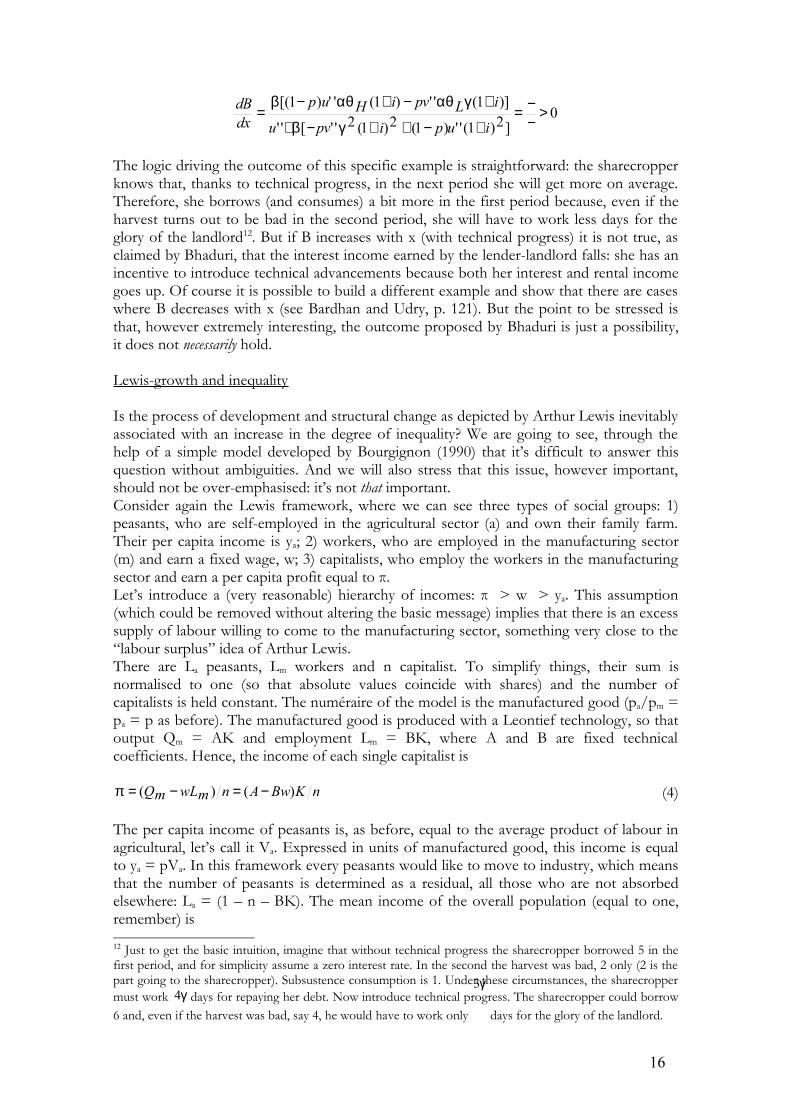
The logic driving the outcome of this specific example is straightforward: the sharecropperknows that, thanks to technical progress, in the next period she will get more on average.Therefore, she borrows (and consumes) a bit more in the first period because, even if theharvest turns out to be bad in the second period, she will have to work less days for theglory of the landlord12. But if B increases with x (with technical progress) it is not true, asclaimed by Bhaduri, that the interest income earned by the lender-landlord falls: she has anincentive to introduce technical advancements because both her interest and rental incomegoes up. Of course it is possible to build a different example and show that there are caseswhere B decreases with x (see Bardhan and Udry, p. 121). But the point to be stressed isthat, however extremely interesting, the outcome proposed by Bhaduri is just a possibility,it does not necessarily hold.

Lewis-growth and inequality

Is the process of development and structural change as depicted by Arthur Lewis inevitablyassociated with an increase in the degree of inequality? We are going to see, through thehelp of a simple model developed by Bourgignon (1990) that it’s difficult to answer thisquestion without ambiguities. And we will also stress that this issue, however important,should not be over-emphasised: it’s not that important.Consider again the Lewis framework, where we can see three types of social groups: 1)peasants, who are self-employed in the agricultural sector (a) and own their family farm.Their per capita income is ya; 2) workers, who are employed in the manufacturing sector(m) and earn a fixed wage, w; 3) capitalists, who employ the workers in the manufacturingsector and earn a per capita profit equal to π.Let’s introduce a (very reasonable) hierarchy of incomes: π > w > ya. This assumption(which could be removed without altering the basic message) implies that there is an excesssupply of labour willing to come to the manufacturing sector, something very close to the“labour surplus” idea of Arthur Lewis. There are La peasants, Lm workers and n capitalist. To simplify things, their sum isnormalised to one (so that absolute values coincide with shares) and the number ofcapitalists is held constant. The numéraire of the model is the manufactured good (pa/pm =pa = p as before). The manufactured good is produced with a Leontief technology, so thatoutput Qm = AK and employment Lm = BK, where A and B are fixed technicalcoefficients. Hence, the income of each single capitalist is

nKBwAnmwLmQ )()( −=−=π (4)

The per capita income of peasants is, as before, equal to the average product of labour inagricultural, let’s call it Va. Expressed in units of manufactured good, this income is equalto ya = pVa. In this framework every peasants would like to move to industry, which meansthat the number of peasants is determined as a residual, all those who are not absorbedelsewhere: La = (1 – n – BK). The mean income of the overall population (equal to one,remember) is 12 Just to get the basic intuition, imagine that without technical progress the sharecropper borrowed 5 in thefirst period, and for simplicity assume a zero interest rate. In the second the harvest was bad, 2 only (2 is thepart going to the sharecropper). Subsustence consumption is 1. Under these circumstances, the sharecroppermust work γ4 days for repaying her debt. Now introduce technical progress. The sharecropper could borrow6 and, even if the harvest was bad, say 4, he would have to work only

γ3

days for the glory of the landlord.

16

aVapLmQapQmQy +=+=

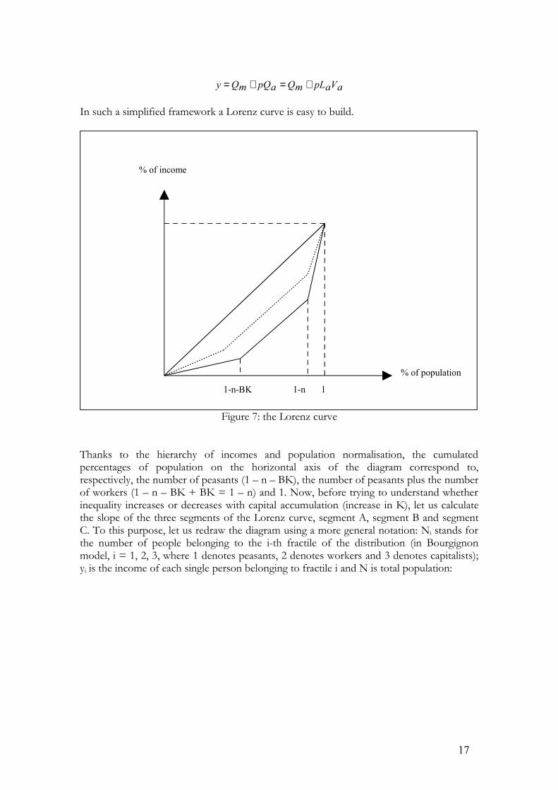
In such a simplified framework a Lorenz curve is easy to build.

Figure 7: the Lorenz curve

Thanks to the hierarchy of incomes and population normalisation, the cumulatedpercentages of population on the horizontal axis of the diagram correspond to,respectively, the number of peasants (1 – n – BK), the number of peasants plus the numberof workers (1 – n – BK + BK = 1 – n) and 1. Now, before trying to understand whetherinequality increases or decreases with capital accumulation (increase in K), let us calculatethe slope of the three segments of the Lorenz curve, segment A, segment B and segmentC. To this purpose, let us redraw the diagram using a more general notation: Ni stands forthe number of people belonging to the i-th fractile of the distribution (in Bourgignonmodel, i = 1, 2, 3, where 1 denotes peasants, 2 denotes workers and 3 denotes capitalists);yi is the income of each single person belonging to fractile i and N is total population:

% of income

% of population

1-n-BK 1-n 1

17

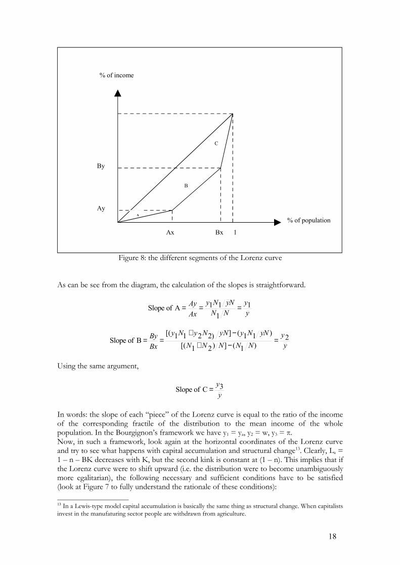
Figure 8: the different segments of the Lorenz curve

As can be see from the diagram, the calculation of the slopes is straightforward.

yy

NNNyNy

AxAy 1

111A of Slope ===

yy

NNNNNNyNyNyNyNy

BxBy 2

)1(])21[(

)11(])2211[(B of Slope =

−+

−+==

Using the same argument,

yy3C of Slope =

In words: the slope of each “piece” of the Lorenz curve is equal to the ratio of the incomeof the corresponding fractile of the distribution to the mean income of the wholepopulation. In the Bourgignon’s framework we have y1 = ya, y2 = w, y3 = π. Now, in such a framework, look again at the horizontal coordinates of the Lorenz curveand try to see what happens with capital accumulation and structural change13. Clearly, La =1 – n – BK decreases with K, but the second kink is constant at (1 – n). This implies that ifthe Lorenz curve were to shift upward (i.e. the distribution were to become unambiguouslymore egalitarian), the following necessary and sufficient conditions have to be satisfied(look at Figure 7 to fully understand the rationale of these conditions):

13 In a Lewis-type model capital accumulation is basically the same thing as structural change. When capitalistsinvest in the manufaturing sector people are withdrawn from agriculture.

% of income

% of population

Bx 1Ax

Ay

By

B

C

A

18

0K

)y( and 0)( ≤∂

∂≥∂

∂ πKyay (5)

In words: the slope of the first “piece” of the Lorenz curve must increase (or stay constant)with capital accumulation, whilst the slope of the last “piece” must decrease (or stayconstant). The economic meaning of this condition is obvious: if income distribution hasto improve, the income of the poorest segment of the population must approach the meanincome from below and the income of the richest segment of the population mustapproach the mean income from above.Well, to check whether those conditions hold we have to write down an explicit formulafor the ratio of the income of both the peasants and the capitalists to the mean income ofthe whole population. Let’s call βa the share of agriculture in national income and αm theprofit share in sector m (which is a constant equal to (1 – Bw/A)); by definition we willhave:

yBKnay

yaVapL

yapQ

a)1( −−

===β

from which we get

BKna

yay

−−=

1β

(6)

As to the profits of the single capitalist, it can be written as

nyam

n

yymQm

n

mQmQ )1(Profits Total

βαα

π−

===

from which we get

nam

y)1( βαπ −

= (7).

From (6) and (7) we can see that conditions (5) are satisfied with certainty if the share ofagriculture in national income increases with K, with capital accumulation and growth. Buthistorically this has never occurred; well on the contrary, the share of agriculture in nationalincome declines with economic growth. So, the reduction of βa will make yπ increase, ascan be seen from (7). What will happen to yya ? As one can see by (6), a priori we can’tsay that much, since the changes in the numerator and the denominator push in oppositedirections. But something less vague can be said if we rewrite (6) more explicitly:

aLa

yay β

=

Now we can say the following: if, during the process of economic growth and structuralchange, the decline in the share of agriculture in national income is faster than that of share

19

of agricultural employment in total employment, then yya will fall. For this condition tobe met, average labour productivity must increase faster than labour productivity inagriculture, which is almost always the case. So, historically, the likely changes to beconsidered are:

0K

)y( and 0)( >∂

∂<∂

∂ πKyay

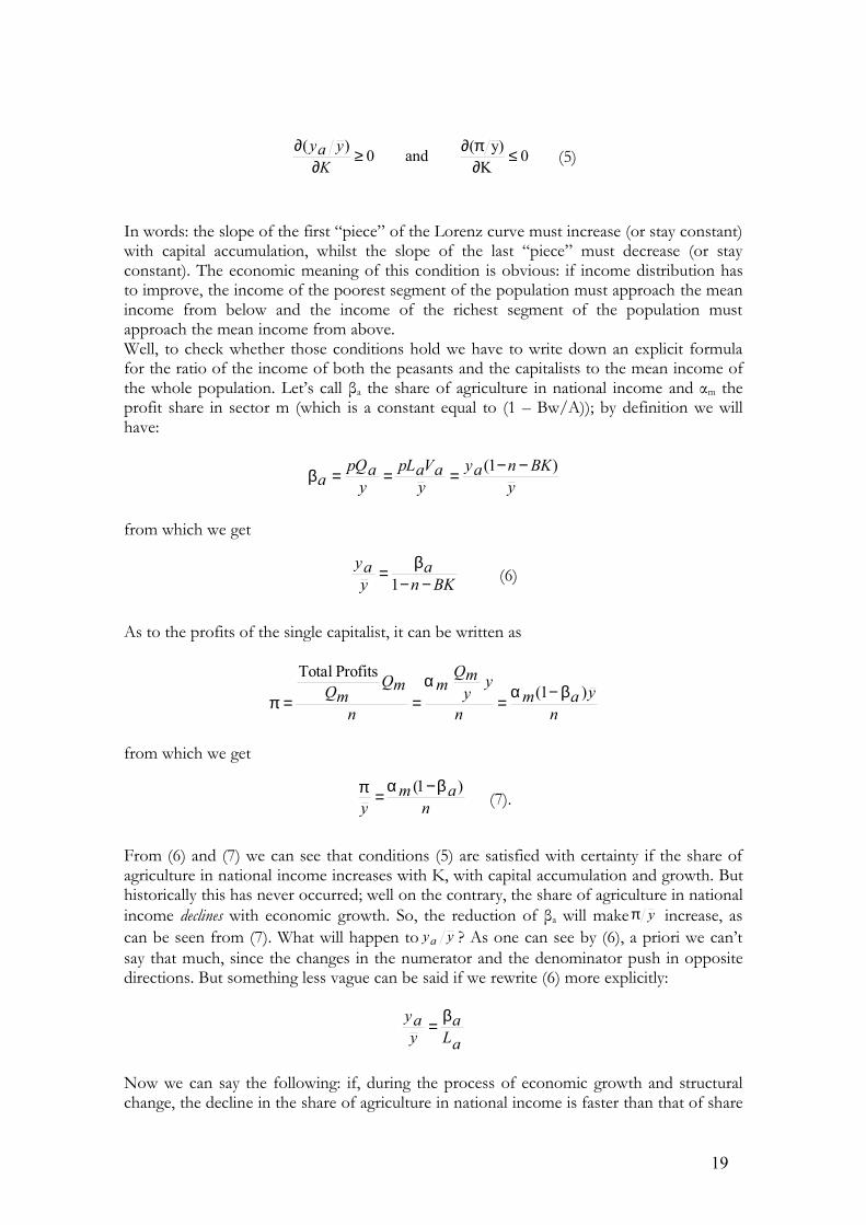
With similar slopes changes we cannot be unambiguous about an increase in inequalitywith economic growth and structural change. The two following diagram show oneambiguous case with intersecting Lorenz curve and a case with unambiguous increase ininequality, both consistent with the slope changes we have just described.

Figure 9: the ambiguous case

% of income

% of population

1-n-BK 1-n 1

20

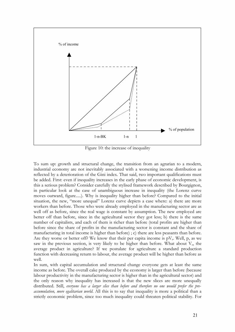
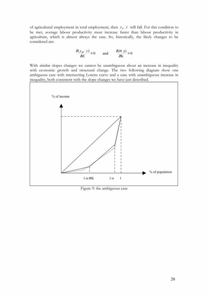
Figure 10: the increase of inequality

To sum up: growth and structural change, the transition from an agrarian to a modern,industrial economy are not inevitably associated with a worsening income distribution asreflected by a deterioration of the Gini index. That said, two important qualifications mustbe added. First: even if inequality increases in the early phase of economic development, isthis a serious problem? Consider carefully the stylised framework described by Bourgignon,in particular look at the case of unambiguous increase in inequality (the Lorenz curvemoves outward, figure.....). Why is inequality higher than before? Compared to the initialsituation, the new, “more unequal” Lorenz curve depicts a case where: a) there are moreworkers than before. Those who were already employed in the manufacturing sector are aswell off as before, since the real wage is constant by assumption. The new employed arebetter off than before, since in the agricultural sector they got less; b) there is the samenumber of capitalists, and each of them is richer than before (total profits are higher thanbefore since the share of profits in the manufacturing sector is constant and the share ofmanufacturing in total income is higher than before) ; c) there are less peasants than before.Are they worse or better off? We know that their per capita income is pVa. Well, p, as wesaw in the previous section, is very likely to be higher than before. What about Va, theaverage product in agriculture? If we postulate for agriculture a standard productionfunction with decreasing return to labour, the average product will be higher than before aswell.In sum, with capital accumulation and structural change everyone gets at least the sameincome as before. The overall cake produced by the economy is larger than before (becauselabour productivity in the manufacturing sector is higher than in the agricultural sector) andthe only reason why inequality has increased is that the new slices are more unequallydistributed. Still, everyone has a larger slice than before and therefore no one would prefer the pre-accumulation, more egalitarian world. All this is to say that inequality is more a political than astrictly economic problem, since too much inequality could threaten political stability. For

% of income

% of population

1-n-BK 1-n 1

21

instance, “agricultural policy has been used in Africa to promote a pattern of incomedistribution which is regarded as legitimate and which therefore does not threaten politicalstability. This is an extremely delicate problem in nation-state building in Africa. Someaspects of agricultural pricing policy, particularly the practice of providing uniformguaranteed prices countrywide, have been part of an implicit social contract designed toredress colonial imbalances and ensure that certain ethnic groups with less fertile land andlimited access to markets are not totally excluded” (UNCTAD, Trade and DevelopmentReport 1998). The second consideration relates to what we observed in the previous section: even in thelabour surplus phase the industrial wage is unlikely to be constant because of the pressureexerted by a rising p. It follows that the profit share in the manufacturing sector, instead ofbeing constant as postulated by Bourgignon, is likely to decrease, which in turn produces amove toward more equality.

3. MIGRATIONS: THE HARRIS-TODARO MODEL (1970)

According to the Lewis model the process of industrialisation entails an “automatic”,someway harmonious migration of people from the rural areas to the cities. Can we saymore on this migration process? Can we add, on top of the agricultural and themanufacturing sector, an urban informal sector to the picture? After all, in many poorcountries there is a large urban population engaged in an extremely diverse set of activitiesoutside the direct scrutiny of the state and not covered by labour unions. And is creatingnew employment opportunities in the city always a good idea? Or is there the risk ofproviding people the incentive to move too fast to the city, so as to create all the problemsinevitably associated with the concentration of a large mass of people in a relatively smallarea? After all, many cities in Africa, Latin America and Asia are growing at 5-7 per centper year, which is likely to be above any realistic possibility of giving these people a job.These questions can be addresses through the help of the model developed in 1970 byHarris and Todaro (for the subsequent changes to the original framework, see Bardhan andUdry, 1999). The key institutional assumptions of the model accord pretty well with manyhighly visible features of some developing countries:

- the rural labour market is competitive- the wage paid by modern firms in the city is fixed above the market clearing level,

either because unions’ activities or governmental legislation (for instance minimumwage regulations) or efficiency wage considerations

- there is an informal sector in which urban residents not otherwise employed canearn their living out of activities outside the control of the state and performedusing heir labour force alone (petty trade, craft production, urban agriculture).

Let Lr be the rural population, employed in agriculture on a fixed amount of land.Agricultural output is determined by the standard production function g(Lr) and sold on aworld market at a price normalised to unity. Since the rural labour market is assumed to becompetitive, rural wages will be equal to the marginal productivity of labour:

)(' rLgrw = .

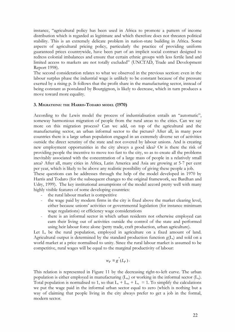
This relation is represented in Figure 11 by the decreasing right-to-left curve. The urbanpopulation is either employed in manufacturing (Lm) or working in the informal sector (Lu).Total population is normalised to 1, so that Lr + Lm + Lu = 1. To simplify the calculationswe put the wage paid in the informal urban sector equal to zero (which is nothing but away of claiming that people living in the city always prefer to get a job in the formal,modern sector.

22

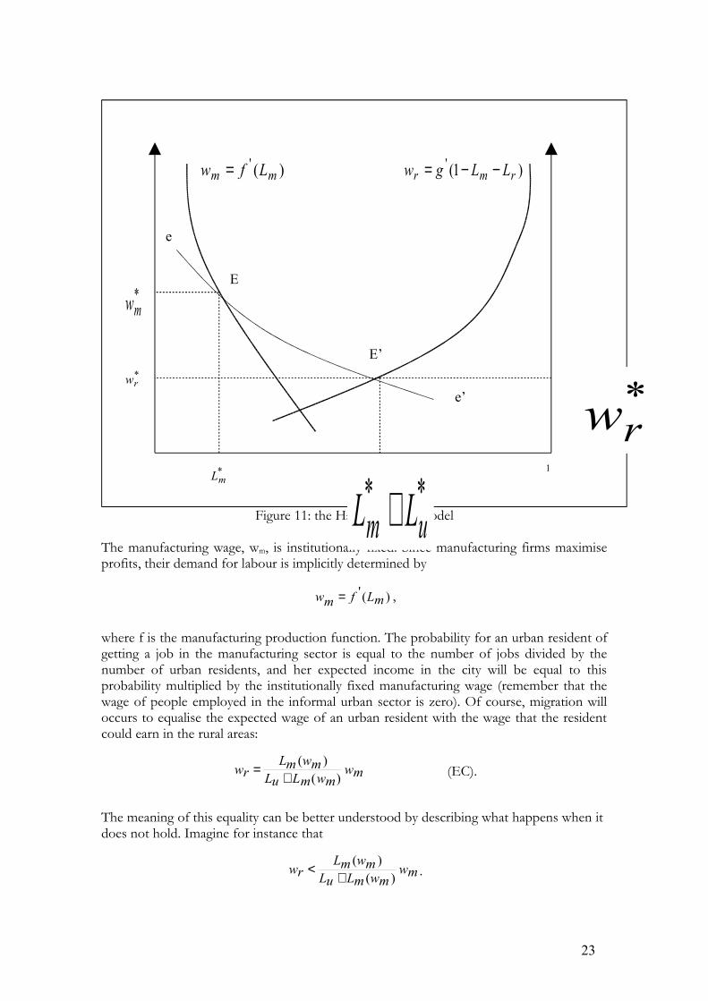
Figure 11: the Harris-Todaro model

The manufacturing wage, wm, is institutionally fixed. Since manufacturing firms maximiseprofits, their demand for labour is implicitly determined by

)(' mLfmw = ,

where f is the manufacturing production function. The probability for an urban resident ofgetting a job in the manufacturing sector is equal to the number of jobs divided by thenumber of urban residents, and her expected income in the city will be equal to thisprobability multiplied by the institutionally fixed manufacturing wage (remember that thewage of people employed in the informal urban sector is zero). Of course, migration willoccurs to equalise the expected wage of an urban resident with the wage that the residentcould earn in the rural areas:

mwmwmLuLmwmLrw )(

)(+

= (EC).

The meaning of this equality can be better understood by describing what happens when itdoes not hold. Imagine for instance that

mwmwmLuLmwmLrw )(

)(+

< .

)(' mm Lfw = )1(' rmr LLgw −−=

*mw

*rw

E

E’

e

e’

1*mL

23

**um LL +

*rw

People living in the rural areas will decide to migrate to the city: But since themanufacturing wage stays constant, Lm will not change and the new urban residents willincrease Lu. At the same time, the reduction of the rural labour force will increase theagricultural marginal product and therefore the agricultural wage. At the end of the storythe equality will be restored. Let’s call the fixed manufacturing wage *

mw . The implicitlydetermined level of manufacturing employment will be *

mL . The equilibrium condition canbe rewritten as

**)*( mwmLmLuLrw =+

In words: the rural wage multiplied by the urban labour force must be equal to a constant.This is the equation of a rectangular hyperbola (like yx = constant): in the diagram, thecurve ee’ represents such an equilibrium locus (of course the hyperbola must pass troughthe point ),( **

mm Lw ). At points E and E’ there is an informal urban sector of size *uL , a rural

population of **1 um LL −− and thus a rural wage of *rw . Since E’ lies on ee’,

**)*( mwmLmLuLrw =+ and expected wages are equalised in the urban and rural sectors. Foran even fuller understanding of the model, let us see diagrammatically what would happenshould the rural wage be less than *

rw .

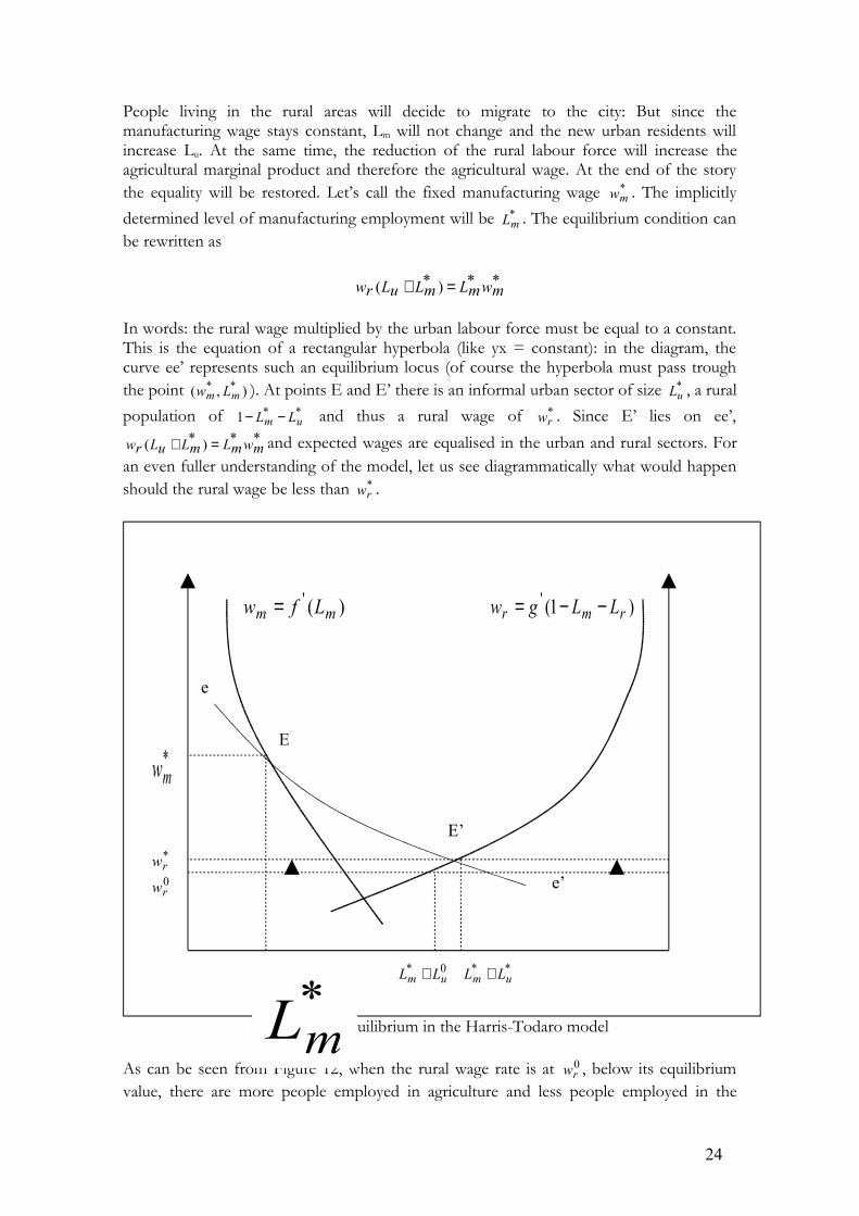
Figure 12: disequilibrium in the Harris-Todaro model

As can be seen from Figure 12, when the rural wage rate is at 0rw , below its equilibrium

value, there are more people employed in agriculture and less people employed in the

)(' mm Lfw = )1(' rmr LLgw −−=

*mw

*rw

E

E’

e

e’

0*um LL + **

um LL +

0rw

24

*mL

informal sector ( **0*umum LLLL +<+ ). But the point ),( 0*0

umr LLw + lies below the equilibriumrectangular hyperbola, which means that

**0*0 )( mmumr LwLLw <+ ,

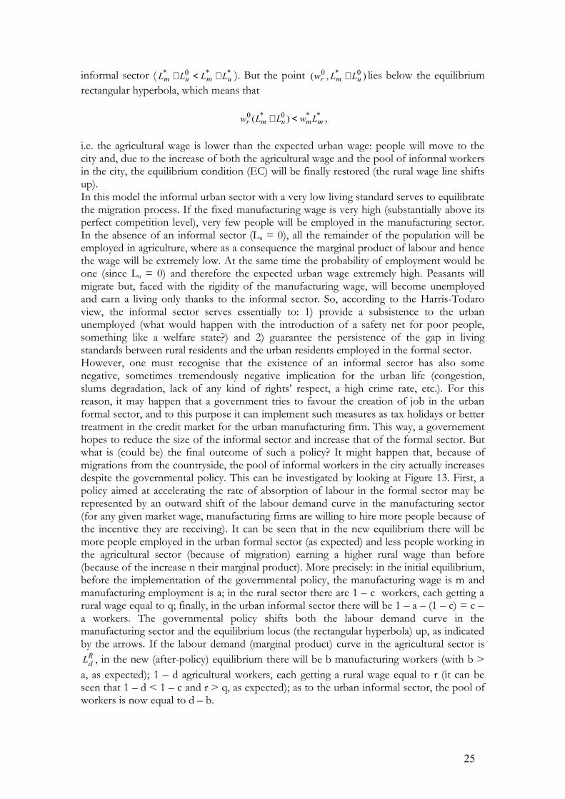
i.e. the agricultural wage is lower than the expected urban wage: people will move to thecity and, due to the increase of both the agricultural wage and the pool of informal workersin the city, the equilibrium condition (EC) will be finally restored (the rural wage line shiftsup).In this model the informal urban sector with a very low living standard serves to equilibratethe migration process. If the fixed manufacturing wage is very high (substantially above itsperfect competition level), very few people will be employed in the manufacturing sector.In the absence of an informal sector (Lu = 0), all the remainder of the population will beemployed in agriculture, where as a consequence the marginal product of labour and hencethe wage will be extremely low. At the same time the probability of employment would beone (since Lu = 0) and therefore the expected urban wage extremely high. Peasants willmigrate but, faced with the rigidity of the manufacturing wage, will become unemployedand earn a living only thanks to the informal sector. So, according to the Harris-Todaroview, the informal sector serves essentially to: 1) provide a subsistence to the urbanunemployed (what would happen with the introduction of a safety net for poor people,something like a welfare state?) and 2) guarantee the persistence of the gap in livingstandards between rural residents and the urban residents employed in the formal sector.However, one must recognise that the existence of an informal sector has also somenegative, sometimes tremendously negative implication for the urban life (congestion,slums degradation, lack of any kind of rights’ respect, a high crime rate, etc.). For thisreason, it may happen that a government tries to favour the creation of job in the urbanformal sector, and to this purpose it can implement such measures as tax holidays or bettertreatment in the credit market for the urban manufacturing firm. This way, a governementhopes to reduce the size of the informal sector and increase that of the formal sector. Butwhat is (could be) the final outcome of such a policy? It might happen that, because ofmigrations from the countryside, the pool of informal workers in the city actually increasesdespite the governmental policy. This can be investigated by looking at Figure 13. First, apolicy aimed at accelerating the rate of absorption of labour in the formal sector may berepresented by an outward shift of the labour demand curve in the manufacturing sector(for any given market wage, manufacturing firms are willing to hire more people because ofthe incentive they are receiving). It can be seen that in the new equilibrium there will bemore people employed in the urban formal sector (as expected) and less people working inthe agricultural sector (because of migration) earning a higher rural wage than before(because of the increase n their marginal product). More precisely: in the initial equilibrium,before the implementation of the governmental policy, the manufacturing wage is m andmanufacturing employment is a; in the rural sector there are 1 – c workers, each getting arural wage equal to q; finally, in the urban informal sector there will be 1 – a – (1 – c) = c –a workers. The governmental policy shifts both the labour demand curve in themanufacturing sector and the equilibrium locus (the rectangular hyperbola) up, as indicatedby the arrows. If the labour demand (marginal product) curve in the agricultural sector isRdL , in the new (after-policy) equilibrium there will be b manufacturing workers (with b >

a, as expected); 1 – d agricultural workers, each getting a rural wage equal to r (it can beseen that 1 – d < 1 – c and r > q, as expected); as to the urban informal sector, the pool ofworkers is now equal to d – b.

25

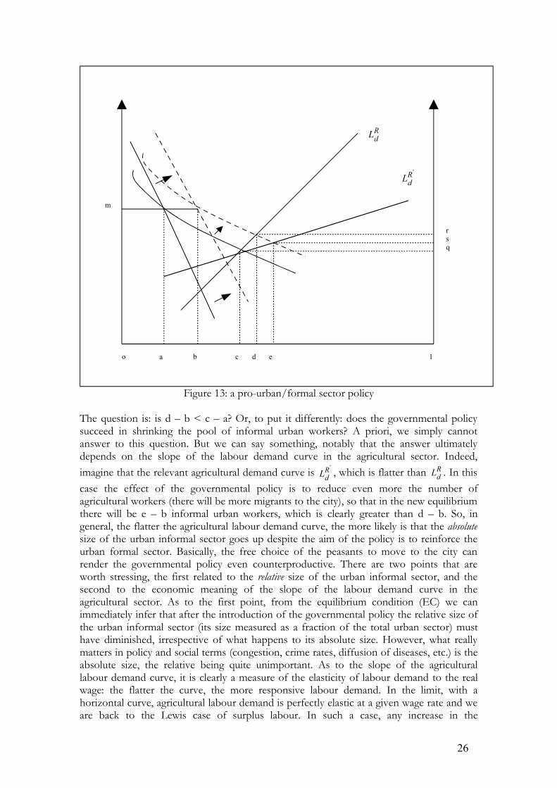
Figure 13: a pro-urban/formal sector policy

The question is: is d – b < c – a? Or, to put it differently: does the governmental policysucceed in shrinking the pool of informal urban workers? A priori, we simply cannotanswer to this question. But we can say something, notably that the answer ultimatelydepends on the slope of the labour demand curve in the agricultural sector. Indeed,imagine that the relevant agricultural demand curve is 'R

dL , which is flatter than RdL . In this

case the effect of the governmental policy is to reduce even more the number ofagricultural workers (there will be more migrants to the city), so that in the new equilibriumthere will be e – b informal urban workers, which is clearly greater than d – b. So, ingeneral, the flatter the agricultural labour demand curve, the more likely is that the absolutesize of the urban informal sector goes up despite the aim of the policy is to reinforce theurban formal sector. Basically, the free choice of the peasants to move to the city canrender the governmental policy even counterproductive. There are two points that areworth stressing, the first related to the relative size of the urban informal sector, and thesecond to the economic meaning of the slope of the labour demand curve in theagricultural sector. As to the first point, from the equilibrium condition (EC) we canimmediately infer that after the introduction of the governmental policy the relative size ofthe urban informal sector (its size measured as a fraction of the total urban sector) musthave diminished, irrespective of what happens to its absolute size. However, what reallymatters in policy and social terms (congestion, crime rates, diffusion of diseases, etc.) is theabsolute size, the relative being quite unimportant. As to the slope of the agriculturallabour demand curve, it is clearly a measure of the elasticity of labour demand to the realwage: the flatter the curve, the more responsive labour demand. In the limit, with ahorizontal curve, agricultural labour demand is perfectly elastic at a given wage rate and weare back to the Lewis case of surplus labour. In such a case, any increase in the

b c d eo 1

m

r s q

RdL

'RdL

26

a

manufacturing, formal employment will be accompanied by an equivalent (in percentageterms) increase in the urban informal employment14. The city is larger than before, but theproportional expansion of the formal and informal sectors has compromised the realisationof the government’s objectives. This general principle can be applied to other policies as well, not necessarily linked toformal labour demand: “ ..policies aimed at directly reducing urban congestion (say, bybuilding more roads), reducing pollution (say, by building a subway), or increasing theprovision of health (say, by building new public hospitals) might all have the paradoxicaleffect of finally worsening these indicators......because fresh migrations in response to theimproved conditions ends up exacerbating the very conditions that the initial policyattempted to ameliorate” (Ray, pp.381-382).

Exercises: 1) What are the effects of technical progress in agriculture in the framework of the

Harris-Todaro model?2) What are the effects of introducing full flexibility of the manufacturing wages

(instead of having them fixed)?3) What are the effects of technical progress in the manufacturing sector?

4. LAND REFORM

• Is the enormous inequality in land holdings bad for agriculture productivity?• If it is, can land rental markets and/or land sale markets spontaneously redress the

balance, reduce such inequality and therefore allow for a productivity increase?• If not, what is the role of a land reform?

Let’s start from the first question. Basically, we can contrast two opposite arguments (inthat they produce contrasting conclusions), a technological argument and an economicargument.The technological argument rests on the notion of economies of scale and leads to theconclusion that large land holdings (and then a certain degree of inequality in land holding)are good for productivity growth in agriculture. Think of those techniques that allowfarmers to achieves a high productivity level:Draft animals. A minimum size of the plot is needed to use them in an economicallyviable way. Imagine you have 2 bullocks, which can be productively employed only on aplot of at least 1 hectare. But you just have a plot of ½ hectare. There would be noproblem if you could rent one of the bullocks out, but such a rental market is usually verythin, for two reason:

• If you rent the bullock out, it could be overworked or mistreated (and you wouldlose value, for you and your sons).

14 This point may be better understood by rewriting the equilibrium condition (EC) as

mmu

r wLL

w1)(

1+

= .

Since neither the manufacturing nor the rural wage change under the labour surplus assumption, formal andinformal labour in the city must grow at the same rate from one equilibrium to the other.

27

• Inside a village (the “natural” dimension of a market, especially when infrastructureand transport facilities are poorly developed) there is often an almost perfectcorrelation in the use of animal power.

Machinery (tractors, pump sets….). Here the minimum size required for efficientownership is even higher (despite the scope for a rental market is somehow better).

So, from a strictly technological point of view, no discussion: large plots of land are moreproductive than small plots of land. Inequality in land holding is good for productivity growth.But now consider the “economic argument”, based on people’s incentives to put as mucheffort as possible in the production process. We will see that, from this perspective, smallholdings (and then a certain degree of equality in land holding) are good for productivity growth.

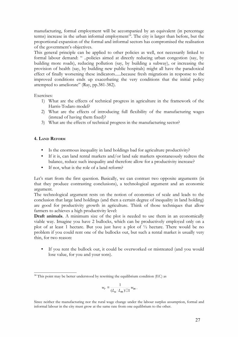
2 agents Landowner

Tenant

risk-neutral

risk–averse

Let us specify the technology in agriculture:

=BG

Y )1( pp

−with G>B

There are two possible arrangements between the landowner and the tenant:

Fixed Rent Contract: the tenant pays R to the landownerSharecropping Contract : the tenant pays a fraction s (sY) to the landowner.

In terms of efficiency (the effort put in the production by the tenant) a fixed rent contractis to be preferred to a sharecropping contract (the reason is easy to understand: if you arethe tenant and have to decide whether to put some extra effort in jour job, what do you doin case of fixed rent contract? And what do you do in case of sharecropping?).So, why do we observe so many sharecropping contracts all around the world?

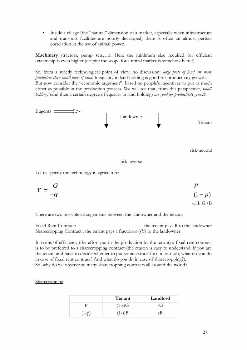
Sharecropping

Tenant LandlordP (1-s)G sG

(1-p) (1-s)B sB

28

29

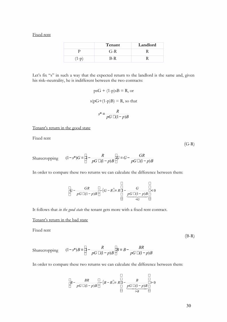
Fixed rent

Tenant LandlordP G-R R

(1-p) B-R R

Let’s fix “s” in such a way that the expected return to the landlord is the same and, givenhis risk–neutrality, he is indifferent between the two contracts:

psG + (1-p)sB = R, or

s(pG+(1-p)B) = R, so that

BppGRs

)1(*

−+=

Tenant’s return in the good state

Fixed rent(G-R)

Sharecropping BppGGRGG

BppGRGs

)1()1(1*)1(

−+−=

−+−=−

In order to compare these two returns we can calculate the difference between them:

( ) 0)1(

1)1(

<

−+−=−−

−+

−

<

G

BppGGRRG

BppGGRG

It follows that in the good state the tenant gets more with a fixed rent contract.

Tenant’s return in the bad state

Fixed rent(B-R)

Sharecropping BppGBRBB

BppGRBs

)1()1(1*)1(

−+−=

−+−=−

In order to compare these two returns we can calculate the difference between them:

( ) 0)1(

1)1(

>

−+−=−−

−+

−

>

B

BppGBRRB

BppGBRB

30

It follows that in the bad state the tenant gets more with a sharecropping arrangement.Overall, the tenant prefers sharecropping because of his risk–aversion. Indeed, if one isrisk-averse she will prefer the option that is better in the bad state. Since, by construction,the landlord is indifferent, the negotiation between the two will come up to asharecropping agreement (with s slightly above s*). So, despite its inefficiency (in terms ofeffort provision), sharecropping is the predominant agrarian agreement.What is the prevailing argument? The argument based on technology (large holdings aregood for agricultural productivity) or the argument based on economic incentives (smallholdings are good for agricultural productivity because in a small plot land can becultivated directly by the farmers and his families, no need to reach any agreement –necessarily: an inefficient sharecropping agreement - with external people. There istherefore a strong incentive to put the maximum possible effort)? The evidence suggests that the incentive argument is more relevant and productivity ishigher on small plots of land (see Ray). However, this raises different policy questions:

Pooling Land and Cooperatives

Drawing on what we have just said, it is tempting to claim that small farmers (who do notneed to respect any agreement with external agents) should pool their lands (basically, forma cooperative) to take advantage of economies of scale. The validity of this argument depends on whether the source of economies of scale lies atthe cultivation (production) level or outside the cultivation process. If it lies outside the cultivation process, for instance because the advantage of poolingcomes from marketing (a big, pooled subject is able to get better prices on the market), thecooperative works: land is cultivated separately in small plots and then the fixed cost ofsetting up a marketing group can be pooled and shared But when the source of economies of scale lies at the production level (say, through the useof tractors), then the incentive problem returns with full force: additional effort by onefarmer leads to additional output, which is then shared among the team. If the farmers failto internalise this positive externality (which requires a complete sense of altruism) effortwill be undersupplied. So, do not expect to see successful wheat or rice cooperatives(sectors where the economies of scales originate at the marketing level), and do not besurprised to discover that collectivisation in China lead to a tremendous reduction inagricultural productivity.

Land Rents and Land Sales So, a more egalitarian distribution of land would increase agricultural productivity andtherefore help sustain the industrialization/development process.A quite natural question arises: why doesn’t a large landowner sell his land splitted intosmaller plots to several small farmers? After all, this should be a very good deal for eachpart of the dealing. To see why:

31

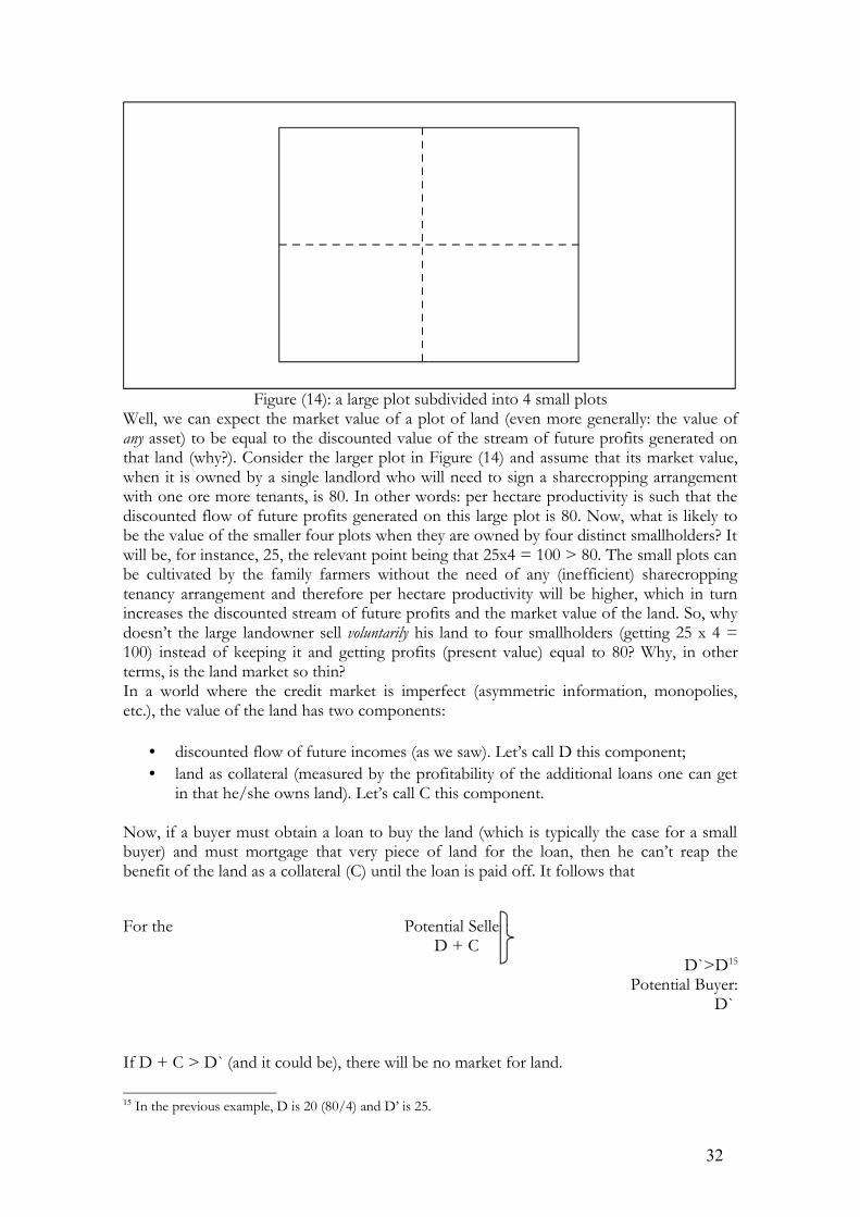
Figure (14): a large plot subdivided into 4 small plotsWell, we can expect the market value of a plot of land (even more generally: the value ofany asset) to be equal to the discounted value of the stream of future profits generated onthat land (why?). Consider the larger plot in Figure (14) and assume that its market value,when it is owned by a single landlord who will need to sign a sharecropping arrangementwith one ore more tenants, is 80. In other words: per hectare productivity is such that thediscounted flow of future profits generated on this large plot is 80. Now, what is likely tobe the value of the smaller four plots when they are owned by four distinct smallholders? Itwill be, for instance, 25, the relevant point being that 25x4 = 100 > 80. The small plots canbe cultivated by the family farmers without the need of any (inefficient) sharecroppingtenancy arrangement and therefore per hectare productivity will be higher, which in turnincreases the discounted stream of future profits and the market value of the land. So, whydoesn’t the large landowner sell voluntarily his land to four smallholders (getting 25 x 4 =100) instead of keeping it and getting profits (present value) equal to 80? Why, in otherterms, is the land market so thin?In a world where the credit market is imperfect (asymmetric information, monopolies,etc.), the value of the land has two components:

• discounted flow of future incomes (as we saw). Let’s call D this component;• land as collateral (measured by the profitability of the additional loans one can get

in that he/she owns land). Let’s call C this component.

Now, if a buyer must obtain a loan to buy the land (which is typically the case for a smallbuyer) and must mortgage that very piece of land for the loan, then he can’t reap thebenefit of the land as a collateral (C) until the loan is paid off. It follows that

For the Potential Seller:D + C

D`>D15

Potential Buyer:D`

If D + C > D` (and it could be), there will be no market for land.

15 In the previous example, D is 20 (80/4) and D’ is 25.

32

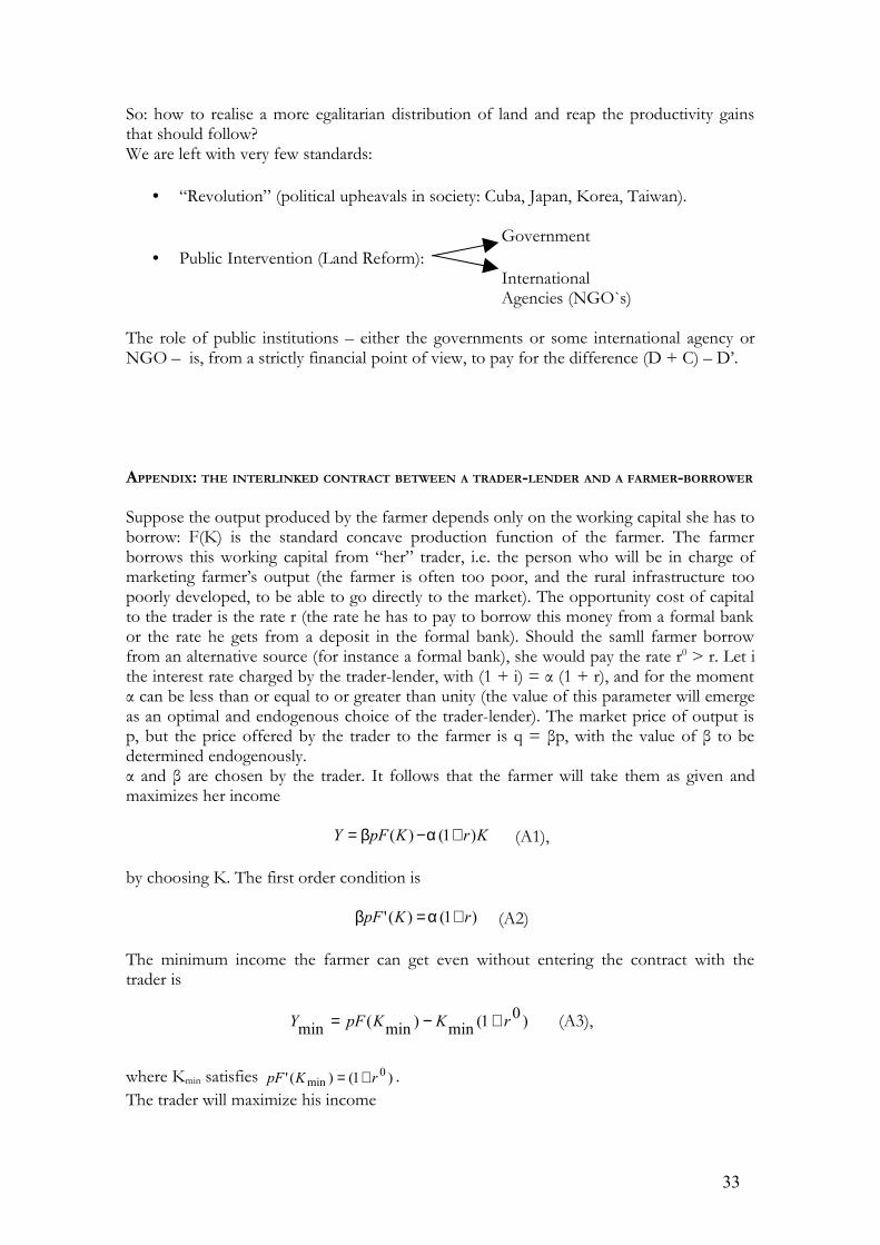
So: how to realise a more egalitarian distribution of land and reap the productivity gainsthat should follow?We are left with very few standards:

• “Revolution” (political upheavals in society: Cuba, Japan, Korea, Taiwan).

Government • Public Intervention (Land Reform):

International Agencies (NGO`s)

The role of public institutions – either the governments or some international agency orNGO – is, from a strictly financial point of view, to pay for the difference (D + C) – D’.

APPENDIX: THE INTERLINKED CONTRACT BETWEEN A TRADER-LENDER AND A FARMER-BORROWER

Suppose the output produced by the farmer depends only on the working capital she has toborrow: F(K) is the standard concave production function of the farmer. The farmerborrows this working capital from “her” trader, i.e. the person who will be in charge ofmarketing farmer’s output (the farmer is often too poor, and the rural infrastructure toopoorly developed, to be able to go directly to the market). The opportunity cost of capitalto the trader is the rate r (the rate he has to pay to borrow this money from a formal bankor the rate he gets from a deposit in the formal bank). Should the samll farmer borrowfrom an alternative source (for instance a formal bank), she would pay the rate r0 > r. Let ithe interest rate charged by the trader-lender, with (1 + i) = α (1 + r), and for the momentα can be less than or equal to or greater than unity (the value of this parameter will emergeas an optimal and endogenous choice of the trader-lender). The market price of output isp, but the price offered by the trader to the farmer is q = βp, with the value of β to bedetermined endogenously.α and β are chosen by the trader. It follows that the farmer will take them as given andmaximizes her income

KrKpFY )1()( +−= αβ (A1),

by choosing K. The first order condition is

)1()(' rKpF += αβ (A2)

The minimum income the farmer can get even without entering the contract with thetrader is

)01(min)min(min rKKpFY +−= (A3),

where Kmin satisfies )1()(' 0min rKpF += .

The trader will maximize his income

33

KrKpF )1)(1()()1(),( +−+−= αββαπ (A4),

by choosing α and β. The trader will have to take into consideration two constraints,known in the literature as the incentive-compatibility constraint and the participation constraint.The former coincides with (A2): it says that the trader will have to chose a value for α andβ by taking into account that his choice will affect farmer’s choice of K and therefore hisown profits. The latter says that the choice of α and β must be such that the farmer doesparticipate to the transaction, instead of being pushed away (if the trader tries to make toomuch money, the farmer will simply go to a formal bank or to some other moneylender).So, formally the problem of the trader is to choose α and β in order to maximise (A4)subject to (A2) and Y ≥ Ymin. One way of solving this problem is to observe that (A4) canbe rewritten (and this is obvious) as the difference between what the trader gets from themarket (net of the cost of capital) and what is left to the farmer:

YKrKpF −+−= ])1()([π

But one thing is sure: the trader will choose α and β so as to press down Y to Ymin (there areno reasons from the point of view of the trader to let the farmer make more money thanwhat is sctrictly needed to induce her participation to the transaction). Since Ymin does notdepend on α and β, it follows that trader will maximize his income when pF(K) – (1+r)K ismaximized, that is to say when pF’(K) = (1+r). But compare this condition with (A2): itmust be α = β. Let us call γ the common optimal value of these two parameters. From (A1)the value of farmer’s income can be rewritten as

]*)1()*([ KrKpFY +−= γ (A5),

where K* is the value of K such that pF’(K*) = 1 + r. Using this propety, (A5) can berewritten as

]*)*(')*([ KKpFKpFY −= γ (A6).

But, as we have already stressed, it must be Y = Ymin, and thus

)*(

)min(*)*(')*(

min)min(')min(

KG

KG

KKFKF

KKFKF=

−

−=γ (A7).

To check whether γ = α = β is greater than or equal to or lower than unity, we have tounderstand the behaviour of the function G and keep in mind that Kmin < K* as r0 > r.Since by definition of G we have G’ = - F’’K > 0, it must be γ = α = β < 1. The economics is relatively simple: the farmer is given an interest discount (i < r), which iscompensated by the underpayment in the output market (q < p).

Exercises

i. What is the effect of a reduction of r0? In the limit, what would happen if r0 = r?Can you give a policy interpretation to this result?

ii. Imagine that your objective is to prevent underpayment to farmers in the outputmarket: what is to be preferred in efficiency terms, an intervention directly in theoutput market or an intervention in the credit market?

34

iii. What would happen in this model if the government decided to launch a programof public works in the city?

Main References

Bhardan, P. and C. Udry, Development Microeconomics, Oxford University Press, 1999;UNCTAD (United Nations Conference on Trade and Development), Trade andDevelopment Report 1998, Geneva, 1998;Ray, D., Development Economics, 1999;

35

36