STAT 312, Fall 2016 Name ________________________________________

Please indicate your registered discussion section in the appropriate table below.

FINAL EXAM

PLEASE SHOW ALL WORK!

Problem Points Grade

1

45

2

45

3

30

4 30

Total

150

LEC 001 TR 9:30-10:45AM 120 Ingraham FISCHER, ISMOR

DIS 311 T 11:00-11:50AM 155 Van Hise Song, Hyebin

DIS 312 T 3:30-4:20PM 387 Van Hise Zhao, Zifeng

LEC 002 TR 1:00-2:15PM 22 Ingraham FISCHER, ISMOR

DIS 321 W 9:55-10:45AM 122 Ingraham Johnston, Liam

DIS 322 W 1:20-2:10PM 486 Van Hise Johnston, Liam

1. An engineer obtains a data set of n = 100 values of a continuous random variable X, that takes its

values in the interval [0,1]. In an effort to fit a model (i.e., “probability density function,” or pdf)

( )f x , she first decides to categorize them into k = 4 equal intervals (or “bins”), shown below.

The first model she tries is the uniform distribution, i.e., 0: ~ Unif [0,1]H X ; see Fig. 1, next page.

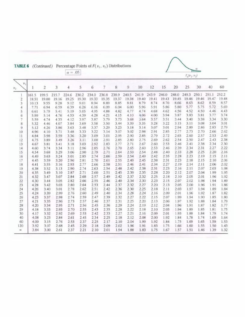
(a) Calculate the appropriate test statistic, and compare it with the corresponding .05 critical score

in the appropriate table. Based on this information, infer a formal conclusion regarding 0H , and

interpret: Does it appear that this distribution is a good fit? Show all work! (15 pts)

The second model she tries is the normal distribution, i.e., 0: ~ (0.5, 0.1)H X N ; see Fig. 2.

(b) Repeat part (a) for this model. Show all work! (15 pts)

The third model she tries uses a linear pdf, i.e., 0: ~ ( ) 2H X f x x ; see Fig. 3.

(c) Repeat part (a) for this model. Show all work! [Hint: Use the fact (via calculus) that the area under

the graph of pdf ( ) 2f x x from a to b is equal to 2 2b a .] (15 pts)

A pdf ( )f x must satisfy two properties: 1) ( ) 0f x for all x, and 2) the total area under its graph is equal to 1.

0 0.25X 0.25 0.50X 0.50 0.75X 0.75 1X

10 20 30 40

0 0.25X 0.25 0.50X 0.50 0.75X 0.75 1X

10 20 30 40

0 0.25X 0.25 0.50X 0.50 0.75X 0.75 1X

10 20 30 40

Fig. 1 Fig. 2

Fig. 3

2. You are working with two numerical random variables X and Y, and obtain a sample data set of

27n points, upon which a simple linear regression is performed. Unfortunately, due to a

computer glitch, the data and almost all of the results are corrupted. All that remains is the following

partial table of summary statistics

Means Variances

x = 314 2

xs = 1250

y = 159 2

ys = 450

and the value of the sample linear correlation coefficient 0.6r . Using this information…

(a) Calculate the value of the sample covariance xys . Show all work. (5 pts)

(b) Determine the equation of the least squares regression line 0 1ˆ ˆY X . Show all work.

(5 pts)

(c) Restore the missing values in the resulting ANOVA table below. [Hint: First calculate the df

column, then SSTotal next.] Show all work. (20 pts)

(d) What is the null hypothesis 0H to which this ANOVA table corresponds? Express symbolically,

and in words. (5 pts)

(e) Make a formal conclusion about whether or not this null hypothesis can be rejected at the .05

significance level. (5 pts)

(f) Interpret your conclusion: What has been demonstrated in this statistical test? Be brief but precise.

(5 pts)

Source df SS MS F-ratio

Regression

Error

Total

3. The following output resulted from a multilinear regression, involving two predictor variables A, B,

and any potential interaction A:B between them.

(a) Which of the estimated regression coefficients are statistically significant at the .05 level?

(5 pts)

(b) Write the formal model for the estimated response Y in terms of A and B. (Be careful.) (5 pts)

(c) Suppose B is a binary variable. If A is held fixed at 98.6, compute the difference in the estimated

responses 1 0ˆ ˆY Y that correspond to B = 1. and B = 0, respectively. Show all work. (15 pts)

(d) Are there any indications that the original might be a poor model? If so, what? Be specific.

(5 pts)

Estimate Std. Error t value Pr(>|t|)

(Intercept) 18.59305 5.11233 3.637 0.00029 ***

A 0.79087 0.48273 1.638 0.10167

B 0.22747 0.19625 1.159 0.24669

A:B 0.03077 0.01846 1.667 0.013584 **

---

Signif. codes: 0 ‘***’ 0.001 ‘**’ 0.01 ‘*’ 0.05 ‘.’ 0.1 ‘ ’ 1

Residual standard error: 10.33 on 996 degrees of freedom

Multiple R-squared: 0.005239, Adjusted R-squared: 0.002243

F-statistic: 1.749 on 3 and 996 DF, p-value: 0.1554

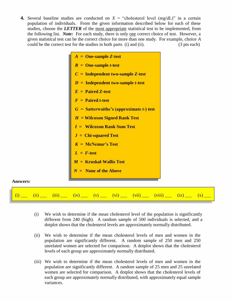
4. Several baseline studies are conducted on X = “cholesterol level (mg/dL)” in a certain population of individuals. From the given information described below for each of these

studies, choose the LETTER of the most appropriate statistical test to be implemented, from

the following list. Note: For each study, there is only one correct choice of test. However, a

given statistical test can be the correct choice for more than one study. For example, choice A

could be the correct test for the studies in both parts (i) and (ii). (3 pts each)

Answers:

(i) We wish to determine if the mean cholesterol level of the population is significantly

different from 240 (high). A random sample of 500 individuals is selected, and a

dotplot shows that the cholesterol levels are approximately normally distributed.

(ii) We wish to determine if the mean cholesterol levels of men and women in the

population are significantly different. A random sample of 250 men and 250

unrelated women are selected for comparison. A dotplot shows that the cholesterol

levels of each group are approximately normally distributed.

(iii) We wish to determine if the mean cholesterol levels of men and women in the

population are significantly different. A random sample of 25 men and 25 unrelated

women are selected for comparison. A dotplot shows that the cholesterol levels of

each group are approximately normally distributed, with approximately equal sample

variances.

(i) ___ (ii) ___ (iii) ___ (iv) ___ (v) ___ (vi) ___ (vii) ___ (viii) ___ (ix) ___ (x) ___

A = One-sample Z-test

B = One-sample t-test

C = Independent two-sample Z-test

D = Independent two-sample t-test

E = Paired Z-test

F = Paired t-test

G = Satterwaithe’s (approximate t-) test

H = Wilcoxon Signed Rank Test

I = Wilcoxon Rank Sum Test

J = Chi-squared Test

K = McNemar’s Test

L = F-test

M = Kruskal-Wallis Test

N = None of the Above

(iv) We wish to determine if the mean cholesterol levels of men and women in the

population are significantly different. A random sample of 25 men and 25 unrelated

women are selected for comparison. A dotplot shows that the cholesterol levels of

each group are approximately normally distributed, but with significantly different

sample variances.

(v) We wish to determine if the mean cholesterol levels of men and women in the

population are significantly different. A random sample of 25 men and 25 unrelated

women are selected for comparison. A dotplot shows that the cholesterol levels of

each group are not normally distributed, but highly skewed.

(vi) We wish to determine if the mean cholesterol levels of husbands and their wives in

the population are significantly different. A random sample of 250 married couples

is selected for comparison between corresponding spouses. A dotplot shows that the

cholesterol levels of each group are approximately normally distributed.

(vii) We wish to determine whether or not there is a significant difference between the

proportions of men and women with high cholesterol. A random sample of 10 men

and 10 unrelated women are selected; each individual is then classified according to

whether or not he/she has high cholesterol, for eventual comparison.

(viii) We wish to determine whether or not there is a significant difference between the

proportions of husbands and their wives with high cholesterol ( 240)X . A random

sample of 250 married couples is selected; each spouse in every couple is then

classified according to whether or not he/she has high cholesterol, for eventual

comparison.

(ix) We wish to determine whether or not the difference between the proportions of men

and women with high cholesterol ( 240)X in the population, is equal to 10%. A

random sample of 250 men and 250 unrelated women are selected; each person is

then classified according to whether or not he/she has high cholesterol, for eventual

comparison.

(x) We wish to determine whether there is a significant difference between the

proportions of individuals in the population whose cholesterol level is low (X < 200),

normal (200 239)X , or high ( 240)X . A random sample of 500 individuals is

selected; each individual is then classified for eventual comparison.

Right-tailed area

Chi-squared scores corresponding to selected right-tailed probabilities of the 2

dfχ distribution

χ 2-score 0 df 1 0.5 0.25 0.10 0.05 0.025 0.010 0.005 0.0025 0.0010 0.0005 0.00025 1 0 0.455 1.323 2.706 3.841 5.024 6.635 7.879 9.141 10.828 12.116 13.412 2 0 1.386 2.773 4.605 5.991 7.378 9.210 10.597 11.983 13.816 15.202 16.588 3 0 2.366 4.108 6.251 7.815 9.348 11.345 12.838 14.320 16.266 17.730 19.188 4 0 3.357 5.385 7.779 9.488 11.143 13.277 14.860 16.424 18.467 19.997 21.517 5 0 4.351 6.626 9.236 11.070 12.833 15.086 16.750 18.386 20.515 22.105 23.681 6 0 5.348 7.841 10.645 12.592 14.449 16.812 18.548 20.249 22.458 24.103 25.730 7 0 6.346 9.037 12.017 14.067 16.013 18.475 20.278 22.040 24.322 26.018 27.692 8 0 7.344 10.219 13.362 15.507 17.535 20.090 21.955 23.774 26.124 27.868 29.587 9 0 8.343 11.389 14.684 16.919 19.023 21.666 23.589 25.462 27.877 29.666 31.427 10 0 9.342 12.549 15.987 18.307 20.483 23.209 25.188 27.112 29.588 31.420 33.221 11 0 10.341 13.701 17.275 19.675 21.920 24.725 26.757 28.729 31.264 33.137 34.977 12 0 11.340 14.845 18.549 21.026 23.337 26.217 28.300 30.318 32.909 34.821 36.698 13 0 12.340 15.984 19.812 22.362 24.736 27.688 29.819 31.883 34.528 36.478 38.390 14 0 13.339 17.117 21.064 23.685 26.119 29.141 31.319 33.426 36.123 38.109 40.056 15 0 14.339 18.245 22.307 24.996 27.488 30.578 32.801 34.950 37.697 39.719 41.699 16 0 15.338 19.369 23.542 26.296 28.845 32.000 34.267 36.456 39.252 41.308 43.321 17 0 16.338 20.489 24.769 27.587 30.191 33.409 35.718 37.946 40.790 42.879 44.923 18 0 17.338 21.605 25.989 28.869 31.526 34.805 37.156 39.422 42.312 44.434 46.508 19 0 18.338 22.718 27.204 30.144 32.852 36.191 38.582 40.885 43.820 45.973 48.077 20 0 19.337 23.828 28.412 31.410 34.170 37.566 39.997 42.336 45.315 47.498 49.632 21 0 20.337 24.935 29.615 32.671 35.479 38.932 41.401 43.775 46.797 49.011 51.173 22 0 21.337 26.039 30.813 33.924 36.781 40.289 42.796 45.204 48.268 50.511 52.701 23 0 22.337 27.141 32.007 35.172 38.076 41.638 44.181 46.623 49.728 52.000 54.217 24 0 23.337 28.241 33.196 36.415 39.364 42.980 45.559 48.034 51.179 53.479 55.722 25 0 24.337 29.339 34.382 37.652 40.646 44.314 46.928 49.435 52.620 54.947 57.217 26 0 25.336 30.435 35.563 38.885 41.923 45.642 48.290 50.829 54.052 56.407 58.702 27 0 26.336 31.528 36.741 40.113 43.195 46.963 49.645 52.215 55.476 57.858 60.178 28 0 27.336 32.620 37.916 41.337 44.461 48.278 50.993 53.594 56.892 59.300 61.645 29 0 28.336 33.711 39.087 42.557 45.722 49.588 52.336 54.967 58.301 60.735 63.104 30 0 29.336 34.800 40.256 43.773 46.979 50.892 53.672 56.332 59.703 62.162 64.555 31 0 30.336 35.887 41.422 44.985 48.232 52.191 55.003 57.692 61.098 63.582 65.999 32 0 31.336 36.973 42.585 46.194 49.480 53.486 56.328 59.046 62.487 64.995 67.435 33 0 32.336 38.058 43.745 47.400 50.725 54.776 57.648 60.395 63.870 66.403 68.865 34 0 33.336 39.141 44.903 48.602 51.966 56.061 58.964 61.738 65.247 67.803 70.289 35 0 34.336 40.223 46.059 49.802 53.203 57.342 60.275 63.076 66.619 69.199 71.706 36 0 35.336 41.304 47.212 50.998 54.437 58.619 61.581 64.410 67.985 70.588 73.118 37 0 36.336 42.383 48.363 52.192 55.668 59.893 62.883 65.739 69.346 71.972 74.523 38 0 37.335 43.462 49.513 53.384 56.896 61.162 64.181 67.063 70.703 73.351 75.924 39 0 38.335 44.539 50.660 54.572 58.120 62.428 65.476 68.383 72.055 74.725 77.319 40 0 39.335 45.616 51.805 55.758 59.342 63.691 66.766 69.699 73.402 76.095 78.709 41 0 40.335 46.692 52.949 56.942 60.561 64.950 68.053 71.011 74.745 77.459 80.094 42 0 41.335 47.766 54.090 58.124 61.777 66.206 69.336 72.320 76.084 78.820 81.475 43 0 42.335 48.840 55.230 59.304 62.990 67.459 70.616 73.624 77.419 80.176 82.851 44 0 43.335 49.913 56.369 60.481 64.201 68.710 71.893 74.925 78.750 81.528 84.223 45 0 44.335 50.985 57.505 61.656 65.410 69.957 73.166 76.223 80.077 82.876 85.591 46 0 45.335 52.056 58.641 62.830 66.617 71.201 74.437 77.517 81.400 84.220 86.954 47 0 46.335 53.127 59.774 64.001 67.821 72.443 75.704 78.809 82.720 85.560 88.314 48 0 47.335 54.196 60.907 65.171 69.023 73.683 76.969 80.097 84.037 86.897 89.670 49 0 48.335 55.265 62.038 66.339 70.222 74.919 78.231 81.382 85.351 88.231 91.022 50 0 49.335 56.334 63.167 67.505 71.420 76.154 79.490 82.664 86.661 89.561 92.371