MPRAMunich Personal RePEc Archive

Internal and International VerticalSpecialization– Estimations For Braziland new Approach to Gravity Models

Joaquim Jose Martins Guilhoto and Jean-Marc Siroen and

Aycil Yucer

Universidade de Sao Paulo, Universite Paris-Dauphine, IRD

2013

Online at http://mpra.ub.uni-muenchen.de/46897/MPRA Paper No. 46897, posted 13. May 2013 21:06 UTC

1

Internal and International Vertical Specialization– Estimations For

Brazil and new Approach to Gravity Models

Joaquim GUILHOTO1

Jean-Marc SIROËN2,3

Aycil YUCER2,3

Abstract:

WTO, OECD with many others, suggest the trade in value-added would be a “better”

measure to understand the impact of trade on employment, growth, production etc. when

import content in exports is important. We use in this work an Input-Output table for

2008, to calculate the value-added exported by Brazilian states. We distinguish the value-

added exported directly by the state itself or indirectly via other states. First, by using

value-added we define the extent of vertical specialization among Brazilian states.

Exported value-added are then used in a gravity model to determine the structure of trade

in value-added terms. We also define a trilateral gravity structure which permits to control

for the vertical specialization between states and to estimate the trade determinants at

three steps: origin state, re-exporter state and importer country.

Keywords: Vertical Specialization, Input-Output Analysis, Gravity Model, Brazil, intra-

national trade

JEL classification: F02, F15, R12, R15

1– Universidade de São Paulo, FEA, NEREUS

2– Université Paris-Dauphine, LEDa, 75775 Paris Cedex 16

3–IRD, UMR225, DIAL, 75010 Paris

2

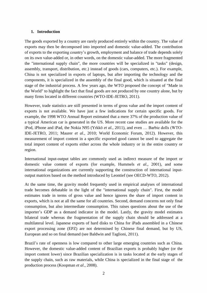
1. Introduction

The goods exported by a country are rarely produced entirely within the country. The value of

exports may then be decomposed into imported and domestic value-added. The contribution

of exports to the exporting country’s growth, employment and balance of trade depends solely

on its own value-added or, in other words, on the domestic value-added. The more fragmented

the "international supply chain", the more countries will be specialized in "tasks" (design,

assembly, transport, distribution, etc.) instead of goods (cars, computers, etc.). For example,

China is not specialized in exports of laptops, but after importing the technology and the

components, it is specialized in the assembly of the final good, which is situated at the final

stage of the industrial process. A few years ago, the WTO proposed the concept of "Made in

the World" to highlight the fact that final goods are not produced by one country alone, but by

many firms located in different countries (WTO-IDE-JETRO, 2011).

However, trade statistics are still presented in terms of gross value and the import content of

exports is not available. We have just a few indications for certain specific goods. For

example, the 1998 WTO Annual Report estimated that a mere 37% of the production value of

a typical American car is generated in the US. More recent case studies are available for the

iPod, iPhone and iPad, the Nokia N95 (Yrkkö et al., 2011), and even … Barbie dolls (WTO-

IDE-JETRO, 2011; Maurer et al., 2010; World Economic Forum, 2012). However, this

measurement of import content in a specific exported good cannot be used to aggregate the

total import content of exports either across the whole industry or in the entire country or

region.

International input-output tables are commonly used as indirect measure of the import or

domestic value content of exports (for example, Hummels et al., 2001), and some

international organizations are currently supporting the construction of international input-

output matrices based on the method introduced by Leontief (see OECD-WTO, 2012).

At the same time, the gravity model frequently used in empirical analyses of international

trade becomes debatable in the light of the "international supply chain". First, the model

estimates trade in terms of gross value and hence ignores the share of import content in

exports, which is not at all the same for all countries. Second, demand concerns not only final

consumption, but also intermediate consumption. This raises questions about the use of the

importer’s GDP as a demand indicator in the model. Lastly, the gravity model estimates

bilateral trade whereas the fragmentation of the supply chain should be addressed at a

multilateral level. Japanese exports of hard disks to China for iPads assembled in a Chinese

export processing zone (EPZ) are not determined by Chinese final demand, but by US,

European and so on final demand (see Baldwin and Taglioni, 2011).

Brazil’s rate of openness is low compared to other large emerging countries such as China.

However, the domestic value-added content of Brazilian exports is probably higher (or the

import content lower) since Brazilian specialization is in tasks located at the early stages of

the supply chain, such as raw materials, while China is specialized in the final stage of the

production process (Koopman et al., 2008).

3

Brazil’s poor performance in terms of openness does not imply a low level of division of

labor along the domestic supply chain. Considering the high heterogeneity of Brazilian

regions in terms of climate, location and factor endowment, there is room for large

specialization differences within Brazil. Yet although inter-state trade statistics are available

(see the previous chapters), they are given in gross value and we have no information on the

shares of own domestic value-added and import content from other states in states' exports.

For example, we saw in the previous chapter that the foreign export capacity of Amazonas is

low, but that São Paulo’s exports may include substantial import content from Amazonas.

The purpose of this paper is precisely to explore the contribution of each Brazilian state to

Brazilian exports and to propose gravity models more in keeping with the "new trade

paradigm" set-up. Section II shows how the geographic fragmentation of the production

process has generated a “new trade paradigm” and what its implications are for traditional

trade analysis. Section III looks into input-output analysis as a new way of measuring trade in

value-added terms and tracking interregional linkages from a value-added point of view.

Section IV explains the method used for the Brazilian Inter-State IO Table built by Guilhoto

(2005, 2010) for 2008, which is the basic source of data for this paper’s analysis and

estimations. Section V provides a descriptive preliminary analysis of the results on the

structure of inter-state vertical specialization for export products. Section VI revises the

gravity model by reworking the theory based on the implications of vertical specialization for

trade. Section VII estimates Brazilian states’ gross exports to the rest of the world, first using

a bilateral gravity model inspired by the traditional approach and then the new measurements

of exports in value-added terms. In section VIII, we take a trilateral gravity model further in

keeping with our theoretical insight in order to measure and control for the impact of inter-

state vertical specialization in states’ exports. Lastly, we present a conclusion on our results.

2. Domestic trade in the light of the “new trade paradigm”

The Made in the World Initiative (MiWi) launched by the WTO is subtitled A Paradigm Shift

to Analyzing Trade. Indeed, the increasing dominance of task specialization over product

specialization has many implications that could be interpreted as a "paradigm shift" (Kuhn,

1962). Theory, statistics, analyses and textbooks currently view the entire gross value of

exports as if it were made up solely of domestic value-added, disregarding the import content

(or foreign value-added) of exports.

The traditional theory of international trade functions in terms of "horizontal" specialization

where countries or firms "become adept at producing particular goods and services from

scratch and then export them," (Hummels et al., 1998). However, we are seeing a growing

geographic fragmentation of the production process in international trade, even though the

phenomenon is not exactly new. The prolific research on the "effective rate of protection"

already refers to this as found, for example, in France, in research on the "Division

Internationale des Processus Productifs" (DIPP).1 We probably owe the term of "vertical

1 Lassudrie-Duchêne, B. (1982)

4

specialization", in contrast to the traditional concept of "horizontal specialization", to Balassa

(1967, p. 97).

However, it is only in recent years that international institutions have turned their attention to

the practical repercussions of this trend on international trade statistics and their

interpretation.2 Two events explain this new interest:

1) The collapse of international trade from mid-2008 to mid-2009 threw the world

suddenly and unexpectedly into deeper world recession. For example, exports fell 38%

for the World and a massive 53% for China in just nine months3. Many explanations

have been advanced for this, such as a trade transaction "credit crunch". Nevertheless,

the fact is that vertical specialization implies that the value-added of a component may

be recorded several times in the trade statistics, i.e. each time it crosses the border for

use in a new stage of the production process. In this case, a $100 drop in national

exports of a final good could cause a drop of $200, $300 or more in world exports4.

2) Case studies that decompose the origin of the value-added of a specific final good

exported outward also reveal very surprising results. These case studies find a

spectacularly weak share of domestic value-added in the value of national exports. The

most striking case is probably the iPod 30 gigabit valued at US$300 in the United

States, previously exported by China for US$150, but with a Chinese value-added

focused on assembly tasks of just US$4 (Dedrik et al., 2009a, 2009 b).

This phenomenon concerns the division of production processes into stages and among

countries until the product arrives on the consumer market as a final good. So countries

become increasingly interconnected with production chains. They are specialized not only in

goods (cars, shoes, etc.), but also in tasks (design, components, assembly procedures, etc.).

The phenomenon is defined more precisely by Hummels et al. (1998) as, "Vertical

specialization occurs when a country uses imported intermediate parts to produce goods it

later exports”. Then, the three conditions need to hold:

(1) A good must be produced in multiple sequential stages,

(2) Two or more countries have to specialize in producing some, but not all stages,

(3) At least one stage must cross an international border more than once.

Incidentally, recognition of vertical specialization prompts a series of questions on the

consistency of the conventional statistical tools and/or on the general concepts of trade

literature. Previously used cross trade measures, which are fairly suitable in a context of

"horizontal" specialization, are becoming more and more unreliable in a world where a final

2 For example, WTO & IDE-JETRO published a report on the issue in 2011. The Organization of Economic

Cooperation and Development (OECD, 2012) supports the position of the World Trade Organization (WTO) in

this area. OECD Secretary-General Angel Gurría highlighted the importance of the subject at the G20 meeting in

Mexico in 2012. And in September 2012, the WTO, OECD and UNCTAD, held a joint seminar with the Chinese

Ministry of Trade on Global Value Chains in Beijing. 3 WTO statistics.

4See, for example, Escaith et al. (2010)

5

good is produced in more than one country or, in general terms, more than one geographic

location. Therefore, the notion of “home” or “origin” of the good is dissociated from the

notion of “exporter”. In particular, the bilateral trade balances measured in gross trade terms

provide very little information on the supply side, because the export values do not reflect the

competitiveness of the exporter entity, but the entire product chain, especially when the

exporter is situated at the final step of the production process. When there is a large volume of

trade in intermediate goods, the use of bilateral gross trade is not appropriate either for the

demand side analysis, since trade flows to the importer country would depend mostly on the

demand of third countries.

The geographic fragmentation of the production process is driven by decreasing trade costs,

policy related or not, such as tariffs, transport and/or communications, etc. The revolutionary

developments in information technologies in the 1990s are an important factor since they have

reduced the cost of communications, enabled remote management and allowed companies to

coordinate long production chains. All of this drives the unbundling of the global economy

(Baldwin, 2006). The emergence of free trade zones, with their advantageous regulations to

attract foreign direct investment (FDI), is also helping to drive this process. The WTO is

making a particular effort to bring down tariffs on the circulation of intermediate products

such as computers, semi-conductors, etc. (e.g. Information Technology Agreement (ITA)).5

Gene Grossman and Esteban Rossi-Hansberg (2006) accentuate the impact of this structural

change on trade and call it “trade in tasks”. Hence, under this new structure of trade costs, the

countries not capable of covering the entire production chain for a good get the chance to

produce at least some of the tasks, provided their production technologies and factor

endowments give them a comparative advantage in a specific task.

On the other hand, these recent dynamics in the structure of trade costs and hence in the trade

structure are also at work in domestic markets. New business management practices have

moreover reduced the cost of coordination within a country. Furthermore, the relatively good

trade integration of domestic markets should make for reduced costs in components trade,

which should facilitate the geographic fragmentation of production stages. Yet, these two

factors are not enough to explain why trade in tasks occurs in domestic markets.

Trade in tasks (or vertical specialization) occurs when differences in countries’ factor

endowments and/or production technology give them the comparative advantage in a specific

task. Nevertheless, under the classical assumptions of traditional trade theories, with factors of

production being perfectly mobile in national markets, endowments are uniform in space. If

that were true, all the regions in a country would have similar comparative advantages and the

company would gain nothing, but face only extra costs from splitting up the production chain

across the country.

However, in reality, neither factor nor good markets are really “perfectly” integrated. Factors

of production are not completely mobile, even within one country. A country’s regions may

5“The Ministerial Declaration on Trade in Information Technology Products (ITA) was concluded at the WTO

Singapore Ministerial Conference in December 1996. The ITA eliminates duties on IT products covered by the

Agreement.” See WTO & IDE-JETRO (2011).

6

differ from in terms of their specializations and production costs. So there could be a gain in

producing tasks in different regions of a country. This is especially true for developing and

emerging markets, such as Latin American countries, India and China, where regional

differences are considerable. On the other hand, transaction costs and the trade integration of

goods markets can also differ across the regions of a country. Wolf (1997) calls this the

spatial non-linearities6 of transaction costs and states that, under these non-linearities, the

production of tasks will be spatially concentrated, instead of being spread out geographically,

and trade in intermediate goods will take place among close entities.

Lastly, trade in tasks is expected to occur in the exporting sectors, since the gain from

economies of scale is another important factor behind specialization in tasks even though

intra-country vertical specialization can occur in a closed economy where internal demand is

large enough to benefit from economies of scale. In that case, trade openness may be a further

incentive to deepen this type of specialization and create a dual dynamic of vertical

specialization. Yet, this internal dimension of specialization driven by trade openness has not

been studied, since many international organizations prioritize inter-country vertical

specialization.

The use of gross trade measures in intra-country trade specialization can trigger a paradigm

change in statistical analysis on two levels: in trade by local entities with world markets and

among themselves. First, the regions specialized in the last stage of the production in the

country seem to export more and so are more integrated into world markets. Second, where

interregional statistics are available to track trade, a good may be counted many times in the

production chain in the internal market. However, the export of the good generally happens

only once and so is counted only once; usually at the last stage of the production chain in the

country. This statistical bias produces extremely high intra national gross trade values for

local entities compared to their actual trade with the rest of the world.

Therefore, a better statistical tool focused on the “origin” and “final destination” of the good

is required to analyze bilateral trade relations at national level as they are at international

level. Measuring trade using the “value-added” approach enables us to approximate the true

origin of exports. This may also be used to determine the value-added contribution at each

stage and hence track the value chain through to the end of the production process. In this

manner, we capture the supply and demand side determinants of trade, such as the "revealed"

competitiveness and comparative advantages of geographic entities that participate at the

different stages of production. The bilateral trade flows, estimated on net value, are

incidentally corrected for the statistical bias created by the multiple accounting of imported

intermediate goods and components embodied in exports.

6 Wolf (1997) believes these non-linearities may be due to “spatial spillovers on the demand or supply side,

spatial clustering of (immobile) factors or an uneven spatial distribution of demand, again coupled with high

transportation costs”.

7

3. Trade in value-added and interregional input-output tables

Pascal Lamy, the WTO's Director General, recently said, "In order to understand the true

nature of trade relationships, we need to know what each country along a global value chain

contributes to the value of a final product. We also need to know how that contribution is

linked to those of other suppliers in other countries coming before and after along the chain.

In order to ensure that trade openness creates jobs overall, as we believe it does, we need to

know how much employment is generated by this value-added factor. The only way to do this

is to measure trade in terms of value-added. This is more easily said than done. But we must

do it."7

Conceptually, the gross value of each exported good includes the exporter’s value-added and

the value-added of the imported inputs incorporated into the good by the foreign and domestic

firms at earlier stages of the production chain. Then, for a traded good, the domestic content

in exports or the value-added by an exporting entity is measured at first glance as the direct

difference between the gross value of the exported good and the imported inputs used to

produce it.8 However, part of the imported inputs may be produced by the exporting country

at earlier stages. Some primary goods and components might be exported and re-imported

after transformation, which complicates the measurement of domestic content in exports. If

we use this logic to find the origin of the inputs used and, by extension, the origin of the

inputs used to produce these inputs and so on, we can decompose the value of a good ( ) in

the value-added ( ) generated across countries or, more broadly, across different

geographic entities (i) participating in the production chain.

∑

Where is the gross value of product p and i is the origin of value-added. However, given

the complexity of re-exporting and re-importing along the production chains and the

multitude of product production processes, it is tricky to measure the origins of value-added

using national accounts. One way of estimating value-added is then to use input-output (IO)

tables. More specifically, interregional input-output (IRIO) tables can be used to estimate the

value-added in traded goods since, unlike standard IO tables, they can track the geographic

path of the production chain and the inter-linkages among regions.

Basically, IO tables were introduced in the 18th

century by François Quesnay’s Tableau

Économique. They were subsequently developed by Wassily Leontief in the 20th

century.

Originally, they were used to represent interrelations between industries within an economy in

terms of supply and use of products in order to analyze the industrial impact of economic

policy, which was a foremost concern post-World War II due to bottlenecks being created in

the economy by full employment, shortage of raw materials, the "dollar gap", etc. One of the

7Lamy Pascal (2012). Global value chains are “binding us together” speech at the WTO-MOFCOM-OECD-

UNCTAD Seminar on Global Value Chains in Beijing on 19 September 2012. 8 In regional input-output work, the flows from one region in a given country to another region of the same

country are referred to as interregional trade (or trade) flows and the terms export and import are used only

when dealing with foreign trade (Miller & Blair, 2009). However, we use the terms export, import and trade for

flows between all types of geographic entities, countries and sub-regions of a country.

8

most famous applications of the IO tables in international trade is the revelation of "Leontief's

paradox" showing that, in contradiction to HOS theory, the United States was not specialized

in capital-intensive goods. Today, IO tables are used across a broader spectrum such as

international and national trade analysis, CO2 emissions, employment issues, etc.

The input-output tables draw on the flows of products taken from the national accounts to

determine the pattern of inter-industry dependencies and their linkages with the final demand

elements in an economy for a reference year. Hence, the production technology is assumed to

be the same for the period of analysis as for the reference table and the input-output

coefficients are assumed to be fixed in the analysis. In the static input-output table, there is a

strict dichotomy between quantities and prices, meaning that production has no effect on

prices and vice versa. Therefore, there is no substitution across inputs and no gain from

economies of scale. Lastly, the supply of labor and capital are unlimited.

Under the above assumptions, input-output tables use the mathematical equality between sales

and purchases to analyze the impact of an increase in sales on purchases. To be more precise,

the input-output table consists of a closed, endogenous part, which basically concerns the

flows of inputs among the industrial sectors of the economy, and the final demand in the

economy, which is "exogenous", since it is independent of the industrial production linkages.

Further, the analysis can be extended with interdependencies among industrial sectors in

different geographic entities, which will then appear in the endogenous part of the

interregional input-output (IRIO) table.

On the sales side (IO table row), the output of sector i ( ) is equal to its supply (sales of

inputs) of intermediate goods to other industries ( where ) for production

(output ) and to domestic purchasers for consumption, e.g. households (final consumption

expenditure), government (government expenditure) and purchasers abroad (exports). The

total demand of the consumer agents is called total final demand ( ).

∑ (1)

Where is a technical coefficient calculated as the ratio of inputs from industry i used in the

total output of industry j. Final demand is exogenous and cannot be predicted by the model.

On the purchase side (IO table column), the output of sector j ( ) is equal to its purchases of

inputs from other industries i ( ) and its purchases from payment sectors ( ) e.g. value-

added (labor, remuneration of capital), imports, etc.

∑ (2)

Since each industrial sector (j) needs purchases from payment sectors in addition to inputs

from industries (i), technical coefficients ( ) have the following features:

9

∑ and ∑

(3)

By writing the equation (1) for all industrial sectors i ( ), we get a system of n linear

equations, which can be represented in matrix form:

and (4)

where

- is a n*1 vector of the n industries’ output

- is an n*n matrix of technical coefficients representing interdependencies between

industries

- is an n*1 vector of final demand

- is the Leontief inverse ( )

Equation 4 is the touchstone of the input-output analysis since it represents the pattern of

inter-industry linkages. It can be used to evaluate the impact of a change in final demand on

total output and further measure, based on the equality from the purchase side, its impact on

the payment sectors, which includes in part the value-added (using Equation 2).

To be more precise, the volume of gross output required to produce final demand is

calculated as follows,

(6)

Or equally, we can approximate it as follows9:

(7)

Then the gross output required to produce will be more than ( ). This can be

explained by round-by-round effects in the input-output analysis. Final demand will be

responded to by the productive sectors that the demand initially addresses. These productive

sectors will produce , with the inputs coming from other sectors ( ). This first round effect

9 An approximation of can be made by generalizing the Neumann series. Consider the identity:

which is equal to:

If ∑ and , then

Hence,

when

10

is called the direct effect of the final demand on the economy. However, the sectors producing

inputs ( ) also need inputs, calculated in the second round as , etc. These secondary,

tertiary and so on round effects are called the indirect effect of demand on the economy10

.

The strength of Leontief’s inverse ( ) is that it captures all these initial, direct and

indirect effects in a single measure.

The next step is to calculate the purchases from the payments sector or, more specifically, the

value-added contribution of the change in final demand. On this point, we need the vector of

value-added coefficients representing the share of value-added in the gross output of each

industrial sector to measure the impact of output on value-added.

Let’s represent the direct value-added contribution for each industrial sector ( in

the reference IO table with a row vector ;11

[ ] (8)

The value-added coefficients ( ) are then equal to the initial value-added contribution of

each industrial sector divided by that sector’s gross output:

[ ] (9)

Where is a diagonal matrix12

and [

]

From the matrix algebra, is a column vector whose elements measure the value-added

generated in each sector in order to produce final demand f. Returning to our example with

final demand , is equal to

(10)

and

is called a sector-demand-to-sector-value-added multiplier. It measures the initial,

direct and indirect value-added contributions of each sector in the total output required to

produce .

10

The definitions of initial, direct and indirect effects can be found in Foundations of IO Analysis by Miller and

Blair (2009). However, in the literature, it is also common to refer to the initial effect as part of the direct effects. 11

Please see Miller & Blair (2009), pp. 243-271, for further details. 12

The “hat” over vector denotes the diagonal matrix whose elements are situated along the diagonal.

Since

Then [

]

11

Interregional input-output (IRIO) tables introduce another aspect of information into the

analysis by extending into interdependencies in space. In IRIO tables, the industrial sectors in

a region also need inputs from other regions in order to produce. Then the basic difference

between standard IO tables and IRIO tables is that the IO tables consider sales to other

regions as exports and account for them in the final demand, while IRIO tables see the

production of the regions as interdependent and therefore endogenous. In IRIO models,

exports, as an element of total final demand, refer to those goods sold to the regions outside

the model’s geographic scope (one region, two regions, etc.) and hence to the purchasers

exogenous to the production sectors.

Let’s take, for example, an IRIO table for two regions (r and s), with each having two

industrial sectors (i and j). In this case, the Leontief inverse is calculated by a two-region

input-output table. The output of industry i in region r is equal to:

(11)

Equation 11 can be generalized in matrix form where A is the interregional input-output

coefficient matrix:

(12)

Where,

A=

[

]

and the output vector x is equal to:

[

]

Therefore, the output required to produce the final demand in one region can be decomposed

by region of origin and industry. The impact of an increase in the output of one region over

the output of other regions is called a “spillover effect” in the literature. To be more precise,

in our example, the output required from sector i in region r ( ) to respond to the final

demand in region s from sector j ( ) is equal to:

(13)

is the element of the interregional Leontief inverse matrix ( ) concerning trade from sector

i in region r to sector j in region s.

12

[

]

Then, the value-added coefficient for industry i in region r is calculated as the ratio of

the industry’s direct value-added to its total output from the reference IRIO table. The indirect

value-added contribution of sector i in region r for the final demand from industrial sector j in

region s ( ) is:

(14)

is the row element of the sector-demand-to-sector-value-added multiplier for

interregional trade from sector i in region r to sector j in region s. In matrix form, sector-

demand-to-sector-value-added multiplier is equal to the following row vector:

(15)

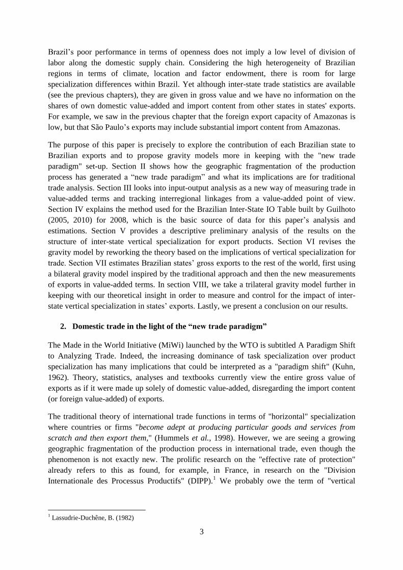
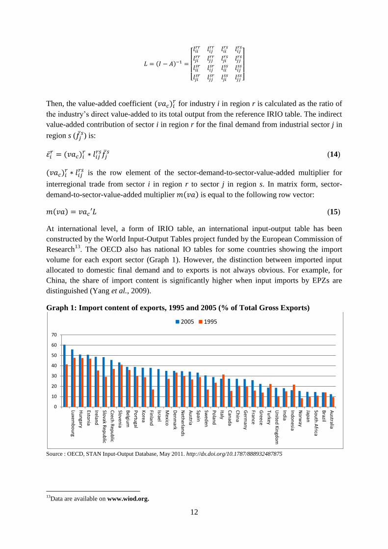
At international level, a form of IRIO table, an international input-output table has been

constructed by the World Input-Output Tables project funded by the European Commission of

Research13

. The OECD also has national IO tables for some countries showing the import

volume for each export sector (Graph 1). However, the distinction between imported input

allocated to domestic final demand and to exports is not always obvious. For example, for

China, the share of import content is significantly higher when input imports by EPZs are

distinguished (Yang et al., 2009).

Graph 1: Import content of exports, 1995 and 2005 (% of Total Gross Exports)

Source : OECD, STAN Input-Output Database, May 2011. http://dx.doi.org/10.1787/888932487875

13

Data are available on www.wiod.org.

0

10

20

30

40

50

60

70

Luxem

bo

urg

Hu

ngary

Eston

ia

Ireland

Slovak R

epu

blic

Czech

Rep

ub

lic

Sloven

ia

Belgiu

m

Po

rtugal

Ko

rea

Finlan

d

Israel

Mexico

Den

mark

Neth

erland

s

Au

stria

Spain

Swed

en

Po

land

Italy

Can

ada

Ch

ina

Germ

any

France

Gree

ce

Turkey

Un

ited

Kin

gdo

m

Ind

ia

Ind

on

esia

No

rway

Japan

Sou

th A

frica

Brazil

Au

stralia

2005 1995

13

In our work, we will concentrate on the interregional input-output table for Brazilian states,

which traces the geographic fragmentation of production across the states and hence shows

the “origin” state of Brazilian foreign exports.

4. Inter-state input-output table (2008)

The Brazilian inter-state input-output system for 27 regions (26 states and the Federal

District) was estimated based on a combination of different sources of data and

methodologies. We first detail the data available to estimate the Brazilian input-output table

and then address the construction of the inter-state input-output system.

The most recent input-output system released by the Brazilian Statistical Office (IBGE) refers

to 2005 (IBGE, 2008). However, using the information available in the Brazilian System of

National Accounts (IBGE, 2010) and the methodology presented by Guilhoto and Sesso Filho

(2005; 2010), we can estimate an input-output system for Brazil for the most recent years

based closely on the Brazilian input-output systems released by the IBGE. From the above, a

national input-output system was estimated for 2008, consisting of national supply and use

tables, giving basic prices, at the level of 56 industries and 110 commodities. The estimated

national input-output system was then used as the basis to estimate the inter-state system for

Brazil based on the methodology presented in Guilhoto et al. (2010).

The steps followed for the estimation of the inter-state system for Brazil can be summarized

as follow14

:

Using information from the IBGE surveys of Agriculture, Industry, Trade, Transport,

Services, and Civil Construction, a first estimate is made of total output by 56

industries and 110 commodities for each of the Brazilian states;

These initial estimates are then balanced to match the total output at the level of 17

industries presented in the Brazilian Regional Accounts (IBGE);

These output estimates are also used to estimate the supply tables for each of the

Brazilian states. The states’ supply tables are estimated in such a way as to be

consistent with the national supply table;

Using information: a) on imports by state, from the Ministry of Development, Industry

and External Trade; b) on tax collection in each state, from the Ministry of Finance

and the State Secretaries of Finance; c) on payments to workers by industry and state,

from the Ministry of Labor and the IBGE Household Survey; d) on value-added

generated at the level of 17 industries, by state, presented in the Brazilian Regional

Accounts (IBGE), the tax, imports, and value-added components are estimated for the

56 industries for each of the Brazilian states, which are also consistent with the value-

added components in the national input-output table;

Using information: a) on exports by each state, from the Ministry of Development,

Industry and External Trade; b) on government spending estimated by the Ministry of

Finance, the States Secretaries of Finance and the IBGE; c) on household spending

14

See Figure 1 in Appendix 1, which summarizes the work needed to estimate the inter-state input-output

system for Brazil.

14

estimated by the Household and Household Consumption Patterns surveys; d) on

investment based on the level of the Civil Construction in each state (IBGE), the

input-output system’s final demand components are estimated for each state, which

are consistent with the national input-output table;

Using cross-industry location quotients for intermediate consumption and simple

location quotients for final demand, a first estimation is made of flows of goods and

services among the Brazilian states;

Using the work done by Vasconcelos and Oliveira (2006), which estimates the flow of

goods among Brazilian states for 1999, and taking into consideration the growth of the

states from 1999 to 2008, a second estimation is made of flows of goods and services

among the Brazilian states;

The third and final estimation of flows of goods and services among the Brazilian

states is made taking into consideration the following: a) the inter-state input-output

system should be consistent with the national table; b) the change in inventories

should be zero when they are zero in the national table; c) the change in inventories in

each state, when related to the total output of the corresponding sector should be in a

range no greater than 30% of this relation found in the national table;

The third estimation produces a commodity by industry inter-state input-output system

for Brazil. The supply tables for each of the states are then used to obtain the industry-

by-industry inter-state system used in this work.

5. Vertical specialization in Brazil

Under the "new trade paradigm", the diversified nature of Brazilian states' characteristics,

such as factor endowments, economic sizes, infrastructures, etc., may drive vertical

specialization at national level. Foreign demand will also drive state specialization in tasks in

order to take advantage of economies of scale. The exported goods are then produced by a

sequence of tasks in which one or more Brazilian states are involved. Hence, the value of

gross exports from one state may partly include the value-added from other states, which

inter-link the foreign trade with inter-state trade.

15

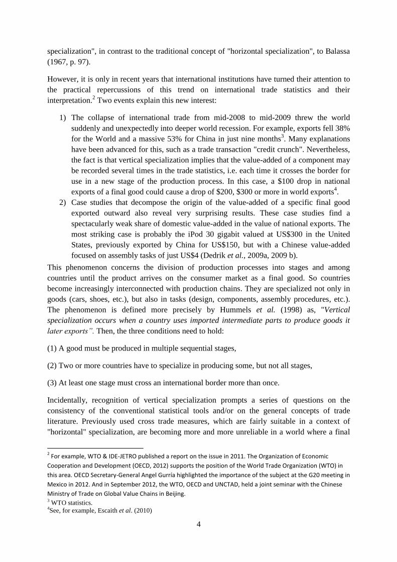
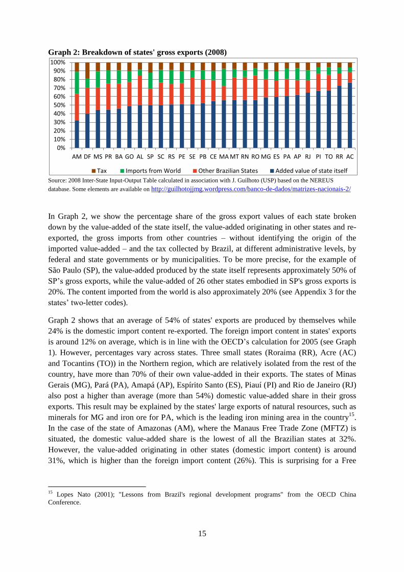
Graph 2: Breakdown of states' gross exports (2008)

Source: 2008 Inter-State Input-Output Table calculated in association with J. Guilhoto (USP) based on the NEREUS

database. Some elements are available on http://guilhotojjmg.wordpress.com/banco-de-dados/matrizes-nacionais-2/

In Graph 2, we show the percentage share of the gross export values of each state broken

down by the value-added of the state itself, the value-added originating in other states and re-

exported, the gross imports from other countries – without identifying the origin of the

imported value-added – and the tax collected by Brazil, at different administrative levels, by

federal and state governments or by municipalities. To be more precise, for the example of

São Paulo (SP), the value-added produced by the state itself represents approximately 50% of

SP’s gross exports, while the value-added of 26 other states embodied in SP's gross exports is

20%. The content imported from the world is also approximately 20% (see Appendix 3 for the

states’ two-letter codes).

Graph 2 shows that an average of 54% of states' exports are produced by themselves while

24% is the domestic import content re-exported. The foreign import content in states' exports

is around 12% on average, which is in line with the OECD’s calculation for 2005 (see Graph

1). However, percentages vary across states. Three small states (Roraima (RR), Acre (AC)

and Tocantins (TO)) in the Northern region, which are relatively isolated from the rest of the

country, have more than 70% of their own value-added in their exports. The states of Minas

Gerais (MG), Pará (PA), Amapá (AP), Espírito Santo (ES), Piauí (PI) and Rio de Janeiro (RJ)

also post a higher than average (more than 54%) domestic value-added share in their gross

exports. This result may be explained by the states' large exports of natural resources, such as

minerals for MG and iron ore for PA, which is the leading iron mining area in the country15

.

In the case of the state of Amazonas (AM), where the Manaus Free Trade Zone (MFTZ) is

situated, the domestic value-added share is the lowest of all the Brazilian states at 32%.

However, the value-added originating in other states (domestic import content) is around

31%, which is higher than the foreign import content (26%). This is surprising for a Free

15

Lopes Nato (2001); "Lessons from Brazil's regional development programs" from the OECD China

Conference.

0%

10%

20%

30%

40%

50%

60%

70%

80%

90%

100%

AM DF MS PR BA GO AL SP SC RS PE SE PB CE MA MT RN RO MG ES PA AP RJ PI TO RR AC

Tax Imports from World Other Brazilian States Added value of state itself

16

Trade Zone, even though it is much higher than the Brazilian states’ average foreign import

content (12%).

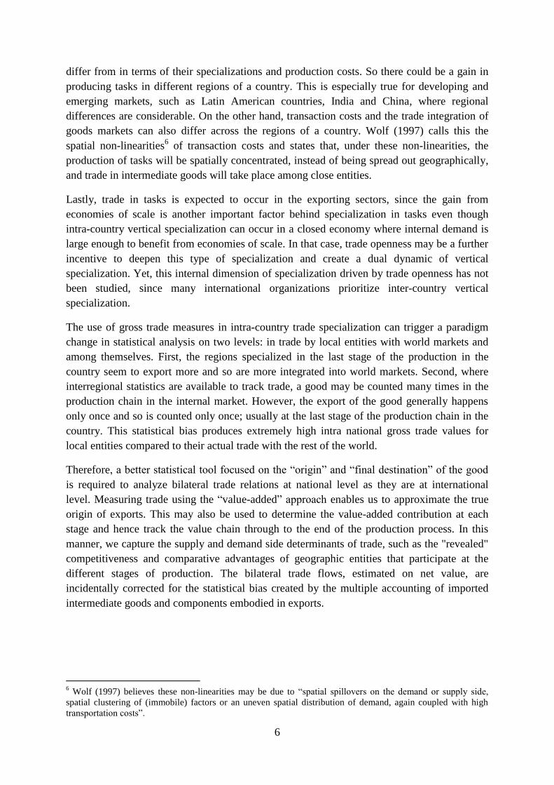
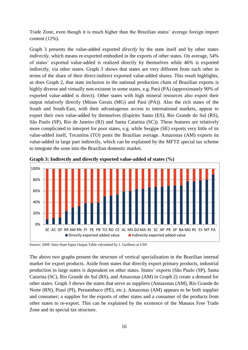
Graph 3 presents the value-added exported directly by the state itself and by other states

indirectly, which means re-exported embodied in the exports of other states. On average, 54%

of states’ exported value-added is realized directly by themselves while 46% is exported

indirectly, via other states. Graph 3 shows that states are very different from each other in

terms of the share of their direct-indirect exported value-added shares. This result highlights,

as does Graph 2, that state inclusion in the national production chain of Brazilian exports is

highly diverse and virtually non-existent in some states, e.g. Pará (PA) (approximately 90% of

exported value-added is direct). Other states with high mineral resources also export their

output relatively directly (Minas Gerais (MG) and Pará (PA)). Also the rich states of the

South and South-East, with their advantageous access to international markets, appear to

export their own value-added by themselves (Espírito Santo (ES), Rio Grande do Sul (RS),

São Paulo (SP), Rio de Janeiro (RJ) and Santa Catarina (SC)). These features are relatively

more complicated to interpret for poor states, e.g. while Sergipe (SE) exports very little of its

value-added itself, Tocantins (TO) posts the Brazilian average. Amazonas (AM) exports its

value-added in large part indirectly, which can be explained by the MFTZ special tax scheme

to integrate the zone into the Brazilian domestic market.

Graph 3: Indirectly and directly exported value-added of states (%)

Source: 2008 Inter-State Input Output Table calculated by J. Guilhoto at USP.

The above two graphs present the structure of vertical specialization in the Brazilian internal

market for export products. Aside from states that directly export primary products, industrial

production in large states is dependent on other states. States’ exports (São Paulo (SP), Santa

Catarina (SC), Rio Grande do Sul (RS), and Amazonas (AM) in Graph 2) create a demand for

other states. Graph 3 shows the states that serve as suppliers (Amazonas (AM), Rio Grande do

Norte (RN), Piauí (PI), Pernambuco (PE), etc.). Amazonas (AM) appears to be both supplier

and consumer; a supplier for the exports of other states and a consumer of the products from

other states to re-export. This can be explained by the existence of the Manaus Free Trade

Zone and its special tax structure.

0%

20%

40%

60%

80%

100%

SE AC DF RR AM RN PI PE PB TO RO CE AL MS GO MA RJ SC AP PR SP BA MG RS ES MT PA

Directly exported added value Indirectly exported added value

17

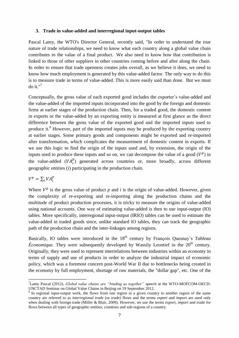
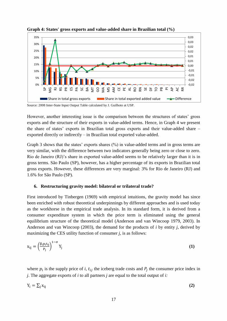
Graph 4: States' gross exports and value-added share in Brazilian total (%)

Source: 2008 Inter-State Input Output Table calculated by J. Guilhoto at USP.

However, another interesting issue is the comparison between the structures of states’ gross

exports and the structure of their exports in value-added terms. Hence, in Graph 4 we present

the share of states’ exports in Brazilian total gross exports and their value-added share –

exported directly or indirectly – in Brazilian total exported value-added.

Graph 3 shows that the states’ exports shares (%) in value-added terms and in gross terms are

very similar, with the difference between two indicators generally being zero or close to zero.

Rio de Janeiro (RJ)’s share in exported value-added seems to be relatively larger than it is in

gross terms. São Paulo (SP), however, has a higher percentage of its exports in Brazilian total

gross exports. However, these differences are very marginal: 3% for Rio de Janeiro (RJ) and

1.6% for São Paulo (SP).

6. Restructuring gravity model: bilateral or trilateral trade?

First introduced by Tinbergen (1969) with empirical intuitions, the gravity model has since

been enriched with robust theoretical underpinnings by different approaches and is used today

as the workhorse in the empirical trade analysis. In its standard form, it is derived from a

consumer expenditure system in which the price term is eliminated using the general

equilibrium structure of the theoretical model (Anderson and van Wincoop 1979, 2003). In

Anderson and van Wincoop (2003), the demand for the products of i by entity j, derived by

maximizing the CES utility function of consumer j, is as follows:

(

)

(1)

where is the supply price of i, the iceberg trade costs and the consumer price index in

j. The aggregate exports of i to all partners j are equal to the total output of i:

∑ (2)

-0,02

-0,02

-0,01

-0,01

0,00

0,01

0,01

0,02

0,02

0,03

0,03

0%

5%

10%

15%

20%

25%

30%

35%

SP

MG RJ

RS

PR ES PA SC BA

MT

GO

MA

MS

AM CE

PE

AL

RO

RN SE DF

TO PB PI

AP

AC

RR

Share in total gross exports Share in total exported added value Difference

18

The above market clearance condition is then used to eliminate the relative price term ( ) in

expenditure equation (1). The equilibrium prices are then:

∑ ( ⁄ )

(3)

Hence, the trade from i to j in equilibrium is:

(

)

(4)

where,

∑ ( ⁄ )

(5)

The above model relies on the assumption that the products exported from i to j are produced

solely in i. In empirical gravity literature, is measured as the gross exports of i to j, while

is measured on a value-added basis by the GDP of entity i. However, under vertical

specialization, the origin of the value-added and the exporter of the good are no longer the

same and the volume of aggregate gross exports is much higher than the amount of domestic

value-added due to the high or increasing import content of exports or, in other words,

intermediate goods imported and re-exported. However, as discussed by Baldwin and

Taglioni (2011), GDP can be used to measure gross output provided the import content of

exports is similar across entities and over time. This is understandable since the ratio of

imported intermediate goods in exports may be considered a constant in the econometric

estimations as long as it is fixed for the whole sample. Nevertheless, trade relation

dependencies are not uniform across countries and world trade today is characterized by a

varying extent of trade in tasks across trade partners. Furthermore, trade in intermediate goods

has grown sharply in recent years.

Another problem in the theoretical model concerns the measurement of j’s expenditure

(Baldwin and Taglioni, 2011). The model assumes that the demand of j is for the final

consumption. Therefore, j’s expenditure is its total income, which is again measured by the

GDP of entity j. However, if j is not the final demand market, but is solely the point where the

good is transformed before being re-exported, then j’s GDP does not reflect its expenditure on

imported goods.

We set out to overcome these two problems in the theoretical model by extending the value

chain from the bilateral frame in the standard gravity model to a trilateral trade relation. With

a trilateral model, we can structure and estimate the trade relation between producer i and

importer j, but we can also control for importer j’s export relations with its partners. So the

exports of i to j can be in final goods, which will be consumed in j or in intermediate goods,

which will be re-exported by j to c (as trade partners of j). For the sake of simplification, we

assume that exports from j to c are solely for final consumption in the destination markets.

19

This trilateral construction takes us one step closer to the real world and it can even be

extended further to a multilateral relation.

j’s demand for products imported from i can then be written as follows:

(

)

( ∑ ) (6)

In Equation 6, unlike the traditional gravity literature, we concentrate on the demand for

outputs produced entirely by exporter i. Hence, instead of the notation – as used in

Equation 1 – we use the total value-added exported from i to j ( )16

. This is a better

measure when there is a high level of vertical specialization. Exports in value-added also

appears to be more in line with the theory, which implicitly assumes that the exported

products originate entirely in the exporter’s country (e.g. Anderson and van Wincoop, 2003),

contrary to the empirical literature, which uses gross exports. Another difference in the

equation is that j’s demand depends not only its own final consumption, but also on its

exports to the rest of the world (c). So the demand addressed to i also covers the intermediate

goods imported by j for re-exportation. Therefore, i exports part of its output directly to its

partner j in response to j’s final demand as measured by its consumer expenditure ( ).

Another part is exported from i indirectly to c via j. The demand of j for this re-exportation is

measured by j’s bilateral gross exports to c ( ), since a partner can be either direct or

indirect at once ( ).

The market clearance condition can then be written as follows:

∑ (7)

where .

The sum of over j should cover the total output of country i either consumed within the

country itself ( ) or exported to j (for final consumption in j or re-export to c). By taking the

sum of Equation 6 on j and using the equality in Equation 7:

∑ ((

)

( ∑ )) (8)

From Equation 8, the price in equilibrium is then equal to:

(

)

(9)

where, is the distance weighted sum of j’s expenditure normalized by j’s price indices:

16

The choice of notation is made in keeping with the IO table literature, where value-added is generally

indexed by two letters (va).

20

(∑ (

)

( ∑ ) )

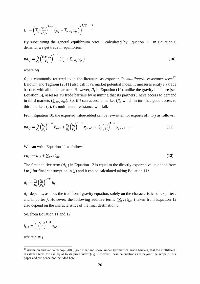
By substituting the general equilibrium price – calculated by Equation 9 – in Equation 6

demand, we get trade in equilibrium:

(

)

( ∑ ) (10)

where .

is commonly referred to in the literature as exporter i’s multilateral resistance term17

.

Baldwin and Taglioni (2011) also call it i’s market potential index. It measures entity i’s trade

barriers with all trade partners. However, in Equation (10), unlike the gravity literature (see

Equation 5), assesses i’s trade barriers by assuming that its partners j have access to demand

in third markets (∑ ). So, if i can access a market ( ), which in turn has good access to

third markets ( ), i’s multilateral resistance will fall.

From Equation 10, the exported value-added can be re-written for exports of i to as follows:

(

)

(

)

(

)

(11)

We can write Equation 11 as follows:

∑ (12)

The first additive term ( ) in Equation 12 is equal to the directly exported value-added from

i to for final consumption in ( ) and it can be calculated taking Equation 11:

(

)

depends, as does the traditional gravity equation, solely on the characteristics of exporter i

and importer j. However, the following additive terms (∑ ) taken from Equation 12

also depend on the characteristics of the final destination c.

So, from Equation 11 and 12:

(

)

where .

17

Anderson and van Wincoop (2003) go further and show, under symmetrical trade barriers, that the multilateral

resistance term for i is equal to its price index ( ). However, these calculations are beyond the scope of our

paper and are hence not included here.

21

is the indirectly exported value-added of i to c. It is indirect since this value-added is re-

exported via to c. Hence, it measures the extent of intermediate trade to from i for final

demand in .

As highlighted by the above theoretical model, the structure of trade in final goods displays a

different pattern to trade in intermediate goods when these are re-exported. The first is shaped

by the bilateral relation between i and j while the latter is trilateral, if not multilateral. In the

next section, we discuss the repercussions of this different trade structure on the empirical

analysis.

7. Bilateral estimation model and results

The traditional empirical trade analysis approach takes the bilateral gravity model, ignoring

the multilateral nature of trade in components. The traditional model estimates bilateral gross

exports by exporter and importer sizes and/or by augmenting the model with their other

observable characteristics along with bilateral distance. In this section, we will take this

approach to understand the limits of the model and then introduce a new trade measure based

on value-added instead of gross exports.

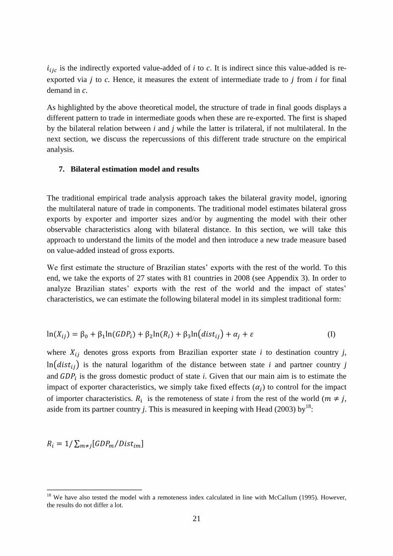
We first estimate the structure of Brazilian states’ exports with the rest of the world. To this

end, we take the exports of 27 states with 81 countries in 2008 (see Appendix 3). In order to

analyze Brazilian states’ exports with the rest of the world and the impact of states’

characteristics, we can estimate the following bilateral model in its simplest traditional form:

( ) (I)

where denotes gross exports from Brazilian exporter state i to destination country j,

( ) is the natural logarithm of the distance between state i and partner country j

and is the gross domestic product of state i. Given that our main aim is to estimate the

impact of exporter characteristics, we simply take fixed effects ( ) to control for the impact

of importer characteristics. is the remoteness of state i from the rest of the world ( ,

aside from its partner country j. This is measured in keeping with Head (2003) by18

:

∑ [ ⁄ ]

18

We have also tested the model with a remoteness index calculated in line with McCallum (1995). However,

the results do not differ a lot.

22

The higher , the more distant state i from countries m ( ) and/or the closer to countries

whose GDPs are relatively small. The more remote the state, the higher trade can be expected

to be between i and its partner j since exporter state i’s access to other markets m is limited.

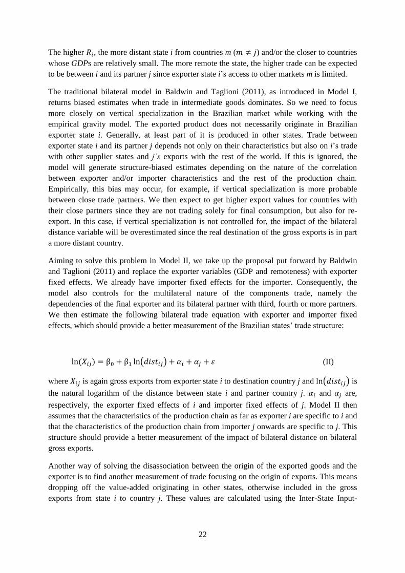
The traditional bilateral model in Baldwin and Taglioni (2011), as introduced in Model I,

returns biased estimates when trade in intermediate goods dominates. So we need to focus

more closely on vertical specialization in the Brazilian market while working with the

empirical gravity model. The exported product does not necessarily originate in Brazilian

exporter state i. Generally, at least part of it is produced in other states. Trade between

exporter state i and its partner j depends not only on their characteristics but also on i’s trade

with other supplier states and j’s exports with the rest of the world. If this is ignored, the

model will generate structure-biased estimates depending on the nature of the correlation

between exporter and/or importer characteristics and the rest of the production chain.

Empirically, this bias may occur, for example, if vertical specialization is more probable

between close trade partners. We then expect to get higher export values for countries with

their close partners since they are not trading solely for final consumption, but also for re-

export. In this case, if vertical specialization is not controlled for, the impact of the bilateral

distance variable will be overestimated since the real destination of the gross exports is in part

a more distant country.

Aiming to solve this problem in Model II, we take up the proposal put forward by Baldwin

and Taglioni (2011) and replace the exporter variables (GDP and remoteness) with exporter

fixed effects. We already have importer fixed effects for the importer. Consequently, the

model also controls for the multilateral nature of the components trade, namely the

dependencies of the final exporter and its bilateral partner with third, fourth or more partners.

We then estimate the following bilateral trade equation with exporter and importer fixed

effects, which should provide a better measurement of the Brazilian states’ trade structure:

( ) (II)

where is again gross exports from exporter state i to destination country j and ( ) is

the natural logarithm of the distance between state i and partner country j. and are,

respectively, the exporter fixed effects of i and importer fixed effects of j. Model II then

assumes that the characteristics of the production chain as far as exporter i are specific to i and

that the characteristics of the production chain from importer j onwards are specific to j. This

structure should provide a better measurement of the impact of bilateral distance on bilateral

gross exports.

Another way of solving the disassociation between the origin of the exported goods and the

exporter is to find another measurement of trade focusing on the origin of exports. This means

dropping off the value-added originating in other states, otherwise included in the gross

exports from state i to country j. These values are calculated using the Inter-State Input-

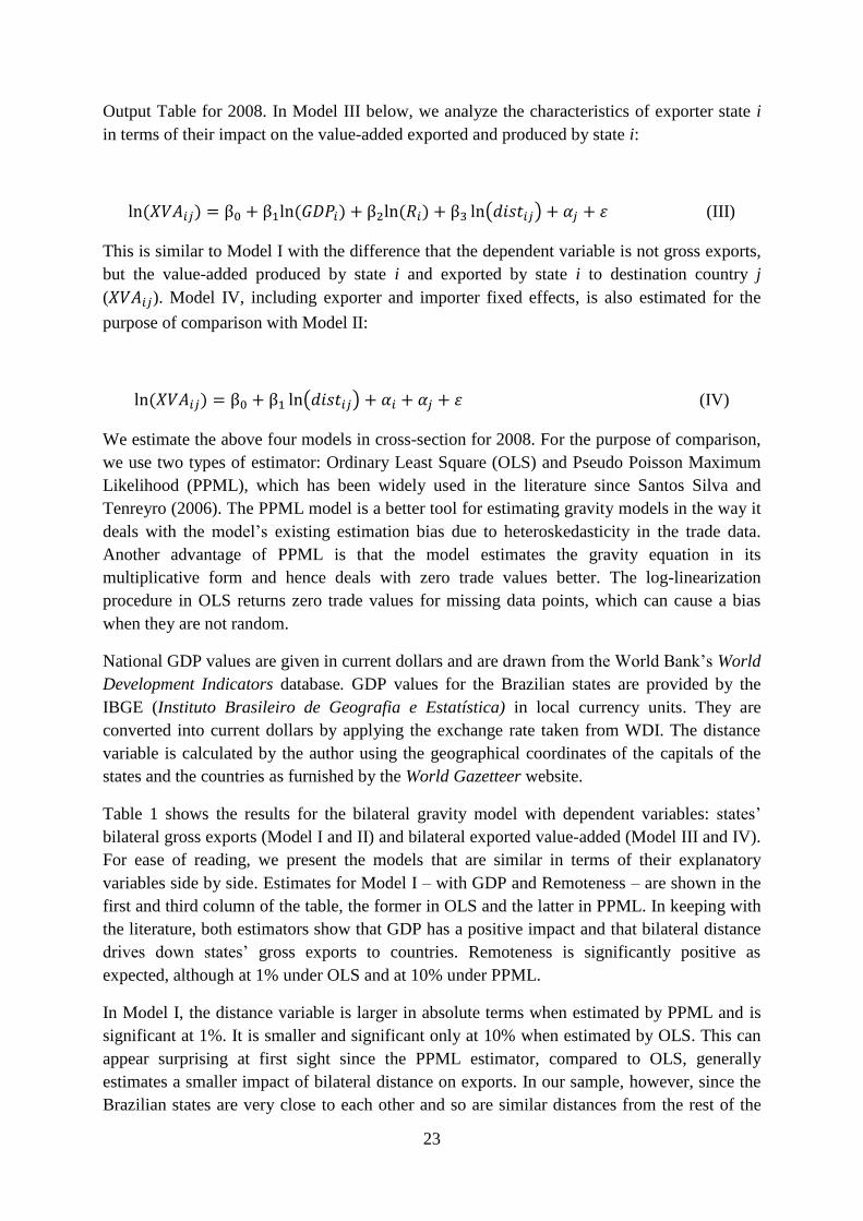
23

Output Table for 2008. In Model III below, we analyze the characteristics of exporter state i

in terms of their impact on the value-added exported and produced by state i:

( ) (III)

This is similar to Model I with the difference that the dependent variable is not gross exports,

but the value-added produced by state i and exported by state i to destination country j

( ). Model IV, including exporter and importer fixed effects, is also estimated for the

purpose of comparison with Model II:

( ) (IV)

We estimate the above four models in cross-section for 2008. For the purpose of comparison,

we use two types of estimator: Ordinary Least Square (OLS) and Pseudo Poisson Maximum

Likelihood (PPML), which has been widely used in the literature since Santos Silva and

Tenreyro (2006). The PPML model is a better tool for estimating gravity models in the way it

deals with the model’s existing estimation bias due to heteroskedasticity in the trade data.

Another advantage of PPML is that the model estimates the gravity equation in its

multiplicative form and hence deals with zero trade values better. The log-linearization

procedure in OLS returns zero trade values for missing data points, which can cause a bias

when they are not random.

National GDP values are given in current dollars and are drawn from the World Bank’s World

Development Indicators database. GDP values for the Brazilian states are provided by the

IBGE (Instituto Brasileiro de Geografia e Estatística) in local currency units. They are

converted into current dollars by applying the exchange rate taken from WDI. The distance

variable is calculated by the author using the geographical coordinates of the capitals of the

states and the countries as furnished by the World Gazetteer website.

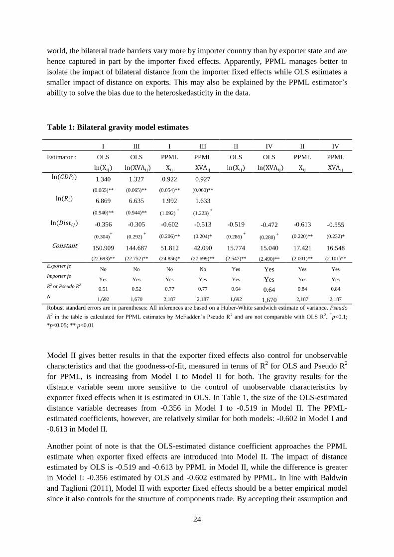
Table 1 shows the results for the bilateral gravity model with dependent variables: states’

bilateral gross exports (Model I and II) and bilateral exported value-added (Model III and IV).

For ease of reading, we present the models that are similar in terms of their explanatory

variables side by side. Estimates for Model I – with GDP and Remoteness – are shown in the

first and third column of the table, the former in OLS and the latter in PPML. In keeping with

the literature, both estimators show that GDP has a positive impact and that bilateral distance

drives down states’ gross exports to countries. Remoteness is significantly positive as

expected, although at 1% under OLS and at 10% under PPML.

In Model I, the distance variable is larger in absolute terms when estimated by PPML and is

significant at 1%. It is smaller and significant only at 10% when estimated by OLS. This can

appear surprising at first sight since the PPML estimator, compared to OLS, generally

estimates a smaller impact of bilateral distance on exports. In our sample, however, since the

Brazilian states are very close to each other and so are similar distances from the rest of the

24

world, the bilateral trade barriers vary more by importer country than by exporter state and are

hence captured in part by the importer fixed effects. Apparently, PPML manages better to

isolate the impact of bilateral distance from the importer fixed effects while OLS estimates a

smaller impact of distance on exports. This may also be explained by the PPML estimator’s

ability to solve the bias due to the heteroskedasticity in the data.

Table 1: Bilateral gravity model estimates

I III I III II IV II IV

Estimator : OLS OLS PPML PPML OLS OLS PPML PPML

1.340 1.327 0.922 0.927

(0.065)** (0.065)** (0.054)** (0.060)**

6.869 6.635 1.992 1.633

(0.940)** (0.944)** (1.092) +

(1.223) +

-0.356 -0.305 -0.602 -0.513 -0.519 -0.472 -0.613 -0.555

(0.304)+ (0.292)

+ (0.206)** (0.204)* (0.286)

+ (0.280)

+ (0.220)** (0.232)*

Constant 150.909 144.687 51.812 42.090 15.774 15.040 17.421 16.548

(22.693)** (22.752)** (24.856)* (27.699)** (2.547)** (2.490)** (2.001)** (2.101)**

Exporter fe No No No No Yes Yes Yes Yes

Importer fe Yes Yes Yes Yes Yes Yes Yes Yes

R2 or Pseudo R2

0.51 0.52 0.77 0.77 0.64 0.64 0.84 0.84

N 1,692 1,670 2,187 2,187 1,692 1,670 2,187 2,187

Robust standard errors are in parentheses: All inferences are based on a Huber-White sandwich estimate of variance. Pseudo

R2 in the table is calculated for PPML estimates by McFadden’s Pseudo R2 and are not comparable with OLS R2. +p<0.1;

*p<0.05; ** p<0.01

Model II gives better results in that the exporter fixed effects also control for unobservable

characteristics and that the goodness-of-fit, measured in terms of R2 for OLS and Pseudo R

2

for PPML, is increasing from Model I to Model II for both. The gravity results for the

distance variable seem more sensitive to the control of unobservable characteristics by

exporter fixed effects when it is estimated in OLS. In Table 1, the size of the OLS-estimated

distance variable decreases from -0.356 in Model I to -0.519 in Model II. The PPML-

estimated coefficients, however, are relatively similar for both models: -0.602 in Model I and

-0.613 in Model II.

Another point of note is that the OLS-estimated distance coefficient approaches the PPML

estimate when exporter fixed effects are introduced into Model II. The impact of distance

estimated by OLS is -0.519 and -0.613 by PPML in Model II, while the difference is greater

in Model I: -0.356 estimated by OLS and -0.602 estimated by PPML. In line with Baldwin

and Taglioni (2011), Model II with exporter fixed effects should be a better empirical model

since it also controls for the structure of components trade. By accepting their assumption and

25

following our comparison between Model I and Model II, we can conclude that the trade

structure of Brazilian states is estimated quite well by PPML even when the exporter fixed

effects are replaced by observable exporter characteristics.

Last but not least, our estimation with the new measurement of trade, based on exported

value-added, slightly reduces the impact of distance and remoteness in absolute terms. The

impact of GDP changes very slightly without any clear conclusion. This result can be

explained by the across-the-board uniformity of states’ vertical specialization. The smaller

impact of distance and remoteness on exported value-added, compared to their impact on

gross exports, may be due to Brazil’s production structure in which the states exporting

primary goods, high in the states’ own value-added, are located in the same region (South-

East: Minas Gerais (MG), Espírito Santo (ES) and Rio de Janeiro (RJ)) where the natural

conditions required for rich natural resources are found.

8. Trilateral estimation model and results

Trade in final goods depends on trade partners’ bilateral relations while the analysis of trade

flows in intermediate goods calls for a multilateral approach to trace the trade relation

throughout the entire value chain. As discussed in the theoretical section, trade in intermediate

goods in a trilateral set-up depends on both the exporter-importer couple’s characteristics and

the origin and demand characteristics in third countries. Hence, the exporter may serve as a

go-between between origin and final demand in third countries and the bilateral trade volume

between the exporter and the importer becomes partly, since it also partly concerns trade in

final consumer goods, the result of this trilateral relation that is typical of components trade.

The traditional bilateral gravity model, even regressed for exports in value-added terms as

conducted in the previous section, does not distinguish the structure of components exports

from the structure of exports in final goods. We therefore focus our analysis on the pattern of

trade in intermediate goods and use an empirical model inspired by Equation 12 above, as

discussed in detail in theoretical section VI. In Equation 12, demand for intermediate goods

from j to i also depends on importer j’s gross exports to the rest of the world (c). Then, from

Equation 12, trade in intermediate goods between i and j for final consumption in c is equal

to;

(

)

where

is the value-added of i indirectly exported to c after transformation in j. In other words, it

is equal to the value of components goods – originating in i – which are embodied in the

exports of j. represents gross exports from to the rest of the world ( ).

Therefore, in the light of the above equation, we can reinterpret the Brazilian states’ trade

structure. In this perspective, Brazilian states' foreign exports depend on their trade relations

with the Brazilian domestic market, namely with other states. To be more precise, bilateral

26

exports from a Brazilian state j to a given country c (e.g. São Paulo to France) also create

demand for components produced in other states i (e.g. Amazonas). Let’s consider that

importer j in the above equation is equally an exporter to c, or to be more precise, a re-

exporter. In the empirical analysis, for easy reading, we denote "i" for the original Brazilian

state, "j" for the re-exporter Brazilian state, and "c", as before, for the foreign country of final

destination or the importer in the model. For example, we consider the Amazonas (i)-São

Paulo (j)-France (c) relation.

The above theoretical model explains only part of the picture. Total trade from state i to state j

is more than the trade of re-exported intermediate goods. However, some intermediate or final

goods can be produced and exported by a given state (state j) independently of other Brazilian

states' production. Yet our objective is to show the structure of trade across vertically

specialized entities and what the implications of disregarding it could be for empirical studies

conducted using the usual approach in the literature, in bilateral terms and gross exports

terms.

First, then, we estimate the following empirical gravity model inspired by the above

theoretical Equation 12;

( )

(I)

– equivalent to in Equation 12 – is measured by the Inter-State IO Table for 2008.

It is equal to the value-added produced in state i and re-exported – as embodied in the

exported goods – by state j to destination country c. An important point of Model I is that the

value-added re-exported from j to c, hence part of the gross exports from j to c, also depends

on the distance of the state of origin i to re-exporter j ( ) and on the characteristics of the

state of origin i. They are controlled with the origin fixed effects ( ). denotes the re-

exporter fixed effects, or the multilateral resistance term for re-exporter j, which refers to

importer j's price index in the theoretical equation.

Model I, however, suffers from an endogeneity problem due to simultaneous causality

between exported value-added and gross exports from j to c. The gross exports from j

to c should drive up i’s value-added re-exported by j. However, the opposite is also true.

obviously represents some share of . In the case of simultaneous causality, the

error term is correlated with the independent variables. So the model is estimated with a

simultaneity bias. In our model, and the error term, which counts for the part of

unexplained by the model, are correlated. So we identify Model I with the exogenous

variables explaining and estimate a reduced form with these exogenous variables. To this

end, we use the traditional gravity model with importer fixed effects, estimating the impact of

observable characteristics for re-exporter state j,

27

( ) ( )

(I’)

Where is the remoteness of state j from importer countries c,

∑ [ ⁄ ]

Model II is equal to the reduced form of Model I with exogenous variables explaining , as

exposed in the traditional gravity Equation I’.19

We then identify Model II as follows:

( ) ( )

(II)

Model II traces the structure of vertically specialized trade in a trilateral set-up. However,

importer fixed effect will also control for the continuation of the value chain, if it exists,

after importer c. In this case, indirect importer c would “re-re-export” the value-added

originating from state i to its trade partners, so consumption would take place in the fourth,

fifth or more destination.

In Model III, we estimate the model using a more general approach based on Baldwin and

Taglioni (2011), where they assume fixed effects to be the best estimation method for the

bilateral gravity model. However, for the trilateral model, we extend their fixed-effects

approach to all three entities in the value chain. In Model III, then, we introduce the fixed

effects for re-exporter state j along with state of origin i and importer country c fixed effects.

( ) ( )

(III)

Model III serves as a good reference. Next, we concentrate on the characteristics of the state

of origin i. To this end, we estimate the above three models by introducing – instead of origin

fixed effects – the observable characteristics of state i.

Hence, the fourth model is equal to:

( )

(IV)

where is the remoteness of state of origin i from other states j. It is measured again in

keeping with Head (2003):

19

In the simultaneous equation estimation, the unbiased impact of the endogenous independent variable ( in

our model) can be calculated by using the algebra on the coefficients estimated separately by the reduced form

equations. However, our objective is not to calculate the impact of on but to structure a gravity model

that correctly estimates the multilateral structure of vertically specialized trade. Hence, the traditional model (I’)

is not estimated, as parameters are not of interest to the scope of our study.

28

∑ [ ⁄ ]

Models V and VI are inspired by the reduced form equation used in Model II:

( ) ( )

(V)

In Model VI, we describe the trade structure by means of the impact of observable

characteristics in states of origin i and re-exporter states s:

( ) ( )

(VI)

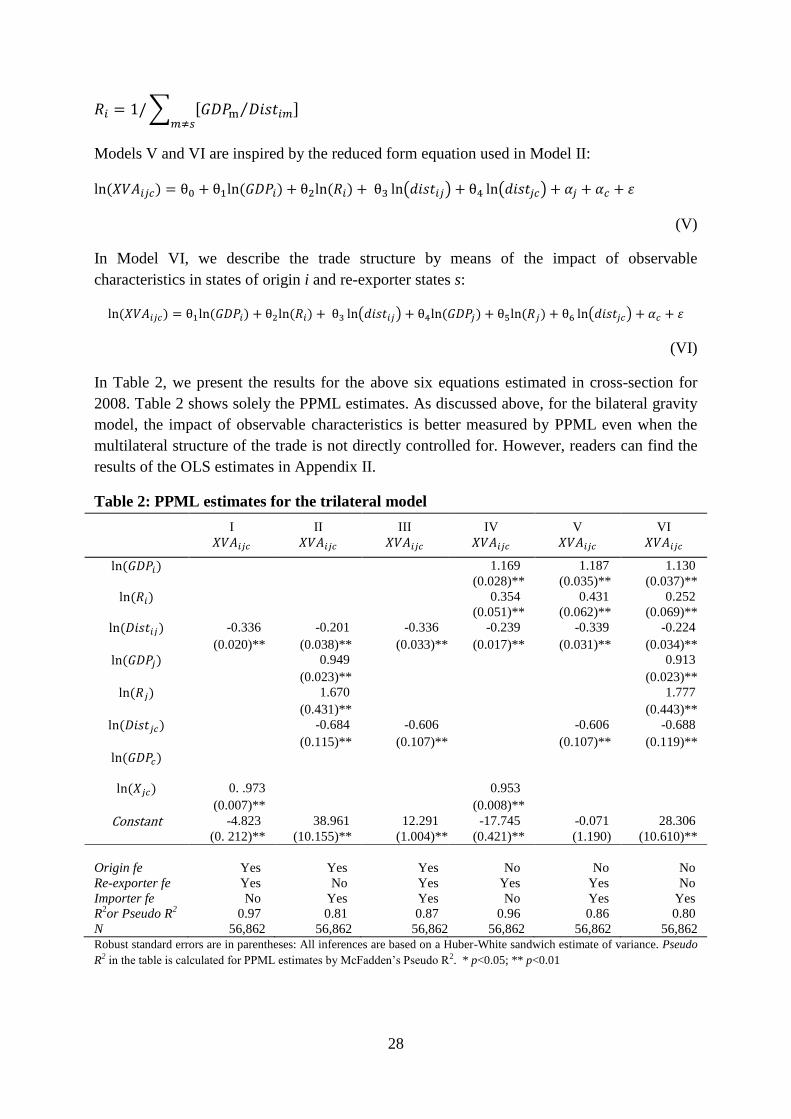
In Table 2, we present the results for the above six equations estimated in cross-section for

2008. Table 2 shows solely the PPML estimates. As discussed above, for the bilateral gravity

model, the impact of observable characteristics is better measured by PPML even when the

multilateral structure of the trade is not directly controlled for. However, readers can find the

results of the OLS estimates in Appendix II.

Table 2: PPML estimates for the trilateral model

I II III IV V VI

1.169 1.187 1.130

(0.028)** (0.035)** (0.037)**

0.354 0.431 0.252

(0.051)** (0.062)** (0.069)**

-0.336 -0.201 -0.336 -0.239 -0.339 -0.224

(0.020)** (0.038)** (0.033)** (0.017)** (0.031)** (0.034)**

0.949 0.913

(0.023)** (0.023)**

1.670 1.777

(0.431)** (0.443)**

-0.684 -0.606 -0.606 -0.688

(0.115)** (0.107)** (0.107)** (0.119)**

0. .973 0.953

(0.007)** (0.008)**

Constant -4.823 38.961 12.291 -17.745 -0.071 28.306

(0. 212)** (10.155)** (1.004)** (0.421)** (1.190) (10.610)**

Origin fe Yes Yes Yes No No No

Re-exporter fe Yes No Yes Yes Yes No

Importer fe No Yes Yes No Yes Yes

R2or Pseudo R

2 0.97 0.81 0.87 0.96 0.86 0.80

N 56,862 56,862 56,862 56,862 56,862 56,862

Robust standard errors are in parentheses: All inferences are based on a Huber-White sandwich estimate of variance. Pseudo

R2 in the table is calculated for PPML estimates by McFadden’s Pseudo R2. * p<0.05; ** p<0.01

29

Model I explains a large part of dependent variable , with Pseudo R2 goodness-of-fit

statistics at around 97%. However, given the simultaneous causality between and

in Model I, the high explanatory power of the model is not surprising. The impact of the

distance from state of origin i to re-exporter state j is significantly different than zero. This

coefficient is smaller compared to the distance impact estimated by bilateral gravity in the

literature.

In Model II, is estimated with the exogenous independent variables. All variables are

significantly different than zero at 1%. Pseudo R2 is very high, at around 81%, although

smaller than it is for Model I. The GDP impact of re-exporter j is around 1. Remoteness

impact is positive, as expected. The impact of distance from state i to state j

( ) is relatively smaller compared to the results found in Model I. On the other hand, the

impact of distance from j to c ( ) has a negative impact, whose extent is in line with the

literature.

Apparently, in the Brazilian example, vertically specialized exports are driven more by the re-

exporter’s distance from the destination country than its distance from the state of origin. This

is an important result, since trade in intermediate goods, which characterizes the first step for

the exports – from state of origin to re-exporter – displays a different pattern to the trade in

the later steps of the value chain. At aggregate level, the bilateral gravity model would not be

able to distinguish these two patterns. It would underestimate the distance impact for final

consumption trade and overestimate it for intermediate goods trade.

Lastly, we present the results for Model III, with fixed effects based on Baldwin and Taglioni

(2011). The coefficient of ( ) is similar to that of Model I. However, this is an expected

result. In Model I, we explain with origin and re-exporter fixed effects along with

bilateral exports ( ) between j and c, which capture a large part of the unobservable bilateral

characteristics between j and c. In Model III, fixed effects for origin, re-exporter and importer

also capture the unobservables with a high Pseudo R2 of around 87%. However, the advantage

of Model III compared to Model I is that it also estimates the impact of distance from re-

exporter j to c. The impact of distance from j to c is -0.606, slightly lower than found in

Model II (-0.688).

The rest of Table 2 concentrates on analyzing the origin characteristics. Model IV is inspired

by our theoretical insights and is also estimated with state of origin i’s observable

characteristics, instead of fixed effects. The impact of is similar to that of Model I; hence

the model looks coherent. The results for state of origin i’s characteristics are significantly

different than zero and bear the expected sign. The impact of the state of origin's GDP is

relatively strong compared to the literature. Hence, it is an important element explaining trade

in a vertical specialization set-up. Remoteness of state of origin i from other states has a

positive impact on . To be more precise, state of origin i’s value-added re-exported by

state j is increasing provided the state of origin is distant from other re-exporter states.

30

In Model V, we estimate the on re-exporter and importer fixed effects; hence the

problem of simultaneity is resolved. The observable characteristics for state of origin i are

always significant after correcting the simultaneity bias. The coefficients are very similar to

Model IV; they are slightly higher in absolute terms for all three variables: GDP of i,

remoteness of i and distance of i from j.

Lastly, we track the entire vertical specialization structure, looking at the impact of observable

characteristics at each step of the value chain. They are in line with previous results. The

coefficient for i’s GDP is significantly different than zero and has a positive impact on its

exported value-added. Re-exporter j’s GDP, however, looks to have a moderate impact

compared with i’s GDP. Hence, the exporter’s output capacity seems to be closely related to

the potential suppliers. Nevertheless, the distance to the consumer or final market seems more

important than the distance to the state of origin. The same holds true for remoteness;

remoteness from final destination country c is more important than remoteness of the state of

origin from the re-exporter.

We believe the above results provide important information as to how the trade structure can

differ between two entities trading in the first step of the value chain and trade partners in the

third or fourth steps of the chain. The bilateral gravity model would ignore this multilateral

character and return biased estimates, under-estimated or over-estimated depending on the

nature of the trade, i.e. whether it is dominated by trade in consumer goods or intermediate

goods. However, this evidence cannot apply across the board because it only concerns

Brazilian states which generally specialize in raw materials and agricultural products located

in the first steps of the supply chain.

9. Conclusion:

Our work discusses the implications of the “new trade paradigm” – reflected in the

geographical fragmentation of the production process – on the traditional statistical and

empirical trade analysis tools. We take a theoretical approach to show that measuring exports

in value-added terms is more appropriate for the gravity model estimates and the model

should be extended to control for the multilateral nature of vertical specialization. Hence, we

propose and estimate a trilateral gravity model frame, which is closer to the reality where

vertical specialization takes the form of a multilateral relation across trade partners.

We first use the Brazilian Inter-State Input-Output table for 2008, to calculate states’ value-

added directly on its own and indirectly via other states. The analysis shows that, with the

exception of states that export natural resources, Brazilian states’ exports are inter-linked by

internal production chains, driven by the demand of rich southern and south-eastern states

(São Paulo (SP), Santa Catarina (SC), etc. ) and supplied by relatively poorer states (Rondonia

(RO), Piauí (PI), etc.). However, our results also find considerable directly exported value-

added for some poor states. The analysis further highlights the special status of the state of

Amazonas (AM) in Brazilian inter-state vertical specialization. Amazonas (AM) is both a

supplier for other states’ exports and a consumer of intermediate goods from other states,

which are then re-exported to the rest of the world.

31

In Section VII, the results of the bilateral gravity model for Brazilian states’ exports show that

GDP impact is fairly similar when the exports are estimated in gross or in value-added terms.

However, the coefficient for distance is smaller and less significant when its impact is

estimated for exported value-added. This finding needs to be interpreted with care because,

given that the sample covers solely Brazilian states’ exports, the bilateral distance variable

varies more by destination country than it does by state of origin.

On the other hand, the trilateral model shows that the structure of exports from origin to re-

exporter and from re-exporter to consumer market is not the same. The distance of the re-

exporter state from the importing partner country has a greater impact than distance from the

state of origin. The re-exporter’s GDP, however, is less important than the state of origin’s

GDP. Therefore, the gravity model estimated using the traditional bilateral approach may

return biased results since it assumes a uniform structure in the trade of consumer goods and

re-exported intermediate goods.

32

References:

Ali-Yrkkö, J., Rouvinen, P., Seppälä, T., Ylä-Anttila, P. (2011). Who Captures Value in

Global Supply Chains? Case Nokia N95 Smartphone. Journal of Industry, Competition And

Trade, 11(3): 263-278.

Anderson, J.E., van Wincoop, E. (2003). Gravity with Gravitas: A Solution to the Border

Puzzle. The American Economic Review, 93(1): 170-192

Balassa, B. (1967). Trade Liberalization among Industrial Countries. New York: McGraw-

Hill.

Baldwin, R. (2006). “Globalisation: the great unbundling(s)”. Paper for the Finnish Prime

Minister’s Office, Economic Council of Finland as part of the EU Presidency.

Baldwin, R., Taglioni, D. (2011). Gravity Chains: Estimating Bilateral Trade Flows when

Parts and Components Trade Is Important. NBER Working Papers, No. 16672.

De Backer, K., Norihiko, Y. (2008). The Measurement of Globalisation Using International

Input-Output. OECD STI Working Paper, DSTI/DOC(2007)8.

Escaith, H., Lindenberg, N., Miroudot, S. (2010). "International Supply Chains and Trade

Elasticity in Times of Global Crisis". WTO, ERSD-2010-08.

Grossman, G.M. and Rossi-Hansberg, E. (2006). The Rise of Offshoring: It’s Not Wine for

Cloth Anymore. Proceedings:59-102.

Guilhoto, J.J.M., Azzoni, C.R., Ichihara,S.M., Kadota, D.K., Haddad, E.A. (2010). "Matriz de

Insumo-Produto do Nordeste e Estados: Metodologia e Resultados". Fortaleza: Banco do

Nordeste do Brasil. ISBN: 978.85.7791.110.3. 289 p.

Guilhoto, J.J.M., Sesso Filho, U.A. (2005). Estimação da Matriz Insumo-Produto a Partir de

Dados Preliminares das Contas Nacionais. Economia Aplicada, 9(2): 277-299.

Guilhoto, J.J.M., Sesso Filho, U.A. (2010). Estimação da Matriz Insumo-Produto Utilizando

Dados Preliminares das Contas Nacionais: Aplicação e Análise de Indicadores Econômicos

para o Brasil em 2005. Economia & Tecnologia. UFPR/TECPAR. 6(23): 53-62.

Head, K. (2003). Gravity for Beginners. Mimeo University of British Columbia, Vancouver,

B.C.

Hummels, D., Rapoport, D., Yi, K.-M. (1998). Vertical Specialization and the Changing

Nature of World Trade. Frbny Economic Policy Review, june.

Hummels, D., Ishii, J., Yi, K.-M. (2001). The nature and growth of vertical specialization in

world trade. Journal of International Economics, 54(1): 75-96.

IBGE (2008). Matriz de Insumo-Produto Brasil: 2000-2005. Rio de Janeiro: Instituto

Brasileiro de Geografia e Estatística – IBGE.

33

IBGE (2010). Sistema de ContasNacionais Brasil: 2004-2008. Rio de Janeiro: Instituto

Brasileiro de Geografia e Estatística – IBGE.

Lassudrie-Duchêne, B. (1982)."Décomposition internationale des processus productifs et

autonomie nationale". Bourguinat H. ed., Internationalisation et autonomie de décision. Paris:

Economica, p. 45-56.

Leontief, W. (1986). Input-Output Economics. 2nd ed., New York: Oxford University Press.

Lopes Neto, A. (2001). “Lessons from Brazil's regional development programs". Paper for

OECD-China Conference. October 2001.

Maurer, A., Degain, C.(2010)."Globalization and trade flows: what you see is not what you

get!". WTO, ERSD-2010-12, June 2010.

McCallum, J. (1995). National Borders Matter: Canada-U.S. Regional Trade Patterns.

American Economic Review, 85(3), p. 615-23.

Miller, R.E., Blair, P.D. (2009). 2nd ed., Input-Output Analysis: Foundations and Extensions.

Cambridge University Press.

OECD (2011). “Import content of exports”. OECD Science, Technology and Industry

Scoreboard 2011 (http://dx.doi.org/10.1787/sti_scoreboard-2011-61-en).

OECD-WTO (2012). "Trade in value-added: concepts, methodologies and challenges". Joint

OECD-WTO note.

Robert, K., Wang, Z., Wei, S.-J., (2008 NBER Working Paper, No.14109).

(http://www.nber.org/papers/w14109)

Wolf, H. (1997). Patterns of Intra- and Inter-State Trade. NBER Working Paper, No. 5939.

World Economic Forum (2012). "The Shifting Geography of Global Value Chains:

Implications for Developing Countries and Trade Policy". World Economic Forum.

WTO-IDE-JETRO (2011). "Trade patterns and global value chains in East Asia: From trade

in goods to trade in tasks". World Trade Organization.

Yang, C., Dietzenbacher, E., Pei, J., Chen, X., Zhu, K., Tang, Z. (2009). "The Bias in

Measuring Vertical Specialization". 17th International Input-Output Conference Sao Paulo,

July 13-17, 2009.

(http://www.iioa.org/pdf/17th%20Conf/Papers/305266464_090531_061106_thebiasinmeasuri

ngverticalspecialization.pdf)

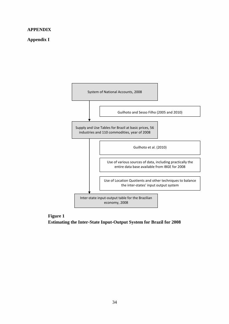
34

APPENDIX

Appendix I

Figure 1

Estimating the Inter-State Input-Output System for Brazil for 2008

System of National Accounts, 2008

Guilhoto and Sesso Filho (2005 and 2010)

Supply and Use Tables for Brazil at basic prices, 56 industries and 110 commodities, year of 2008

Use of Location Quotients and other techniques to balance the inter-states’ input output system

Use of various sources of data, including practically the entire data base available from IBGE for 2008

Inter-state input-output table for the Brazilian economy, 2008

Guilhoto et al. (2010)

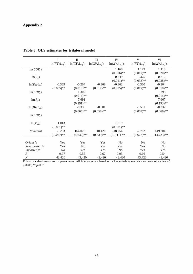
35

Appendix 2

Table 3: OLS estimates for trilateral model

I II III IV V VI

1.168 1.179 1.118

(0.006)** (0.017)** (0.020)**

0.349 0.375 0.212

(0.011)** (0.033)** (0.038)**

-0.369 -0.204 -0.369 -0.362 -0.360 -0.204

(0.005)** (0.018)** (0.017)** (0.005)** (0.017)** (0.018)**

1.302 1.295

(0.014)** (0.014)**

7.691 7.667

(0.191)** (0.193)**

-0.330 -0.501 -0.501 -0.332

(0.065)** (0.058)** (0.059)** (0.066)**

1.013 1.019

(0.001)** (0.001)**

Constant -5.283 164.076 10.420 -18.254 -2.762 149.304

(0 .057)** (4.632)** (0.539)** (0. 111) ** (0.627)** (4.723)**

Origin fe Yes Yes Yes No No No

Re-exporter fe Yes No Yes Yes Yes No

Importer fe No Yes Yes No Yes Yes

R2

0.97 0.55 0.67 0.95 0.66 0.54

N 43,420 43,420 43,420 43,420 43,420 43,420

Robust standard errors are in parentheses: All inferences are based on a Huber-White sandwich estimate of variance.*

p<0.05; ** p<0.01

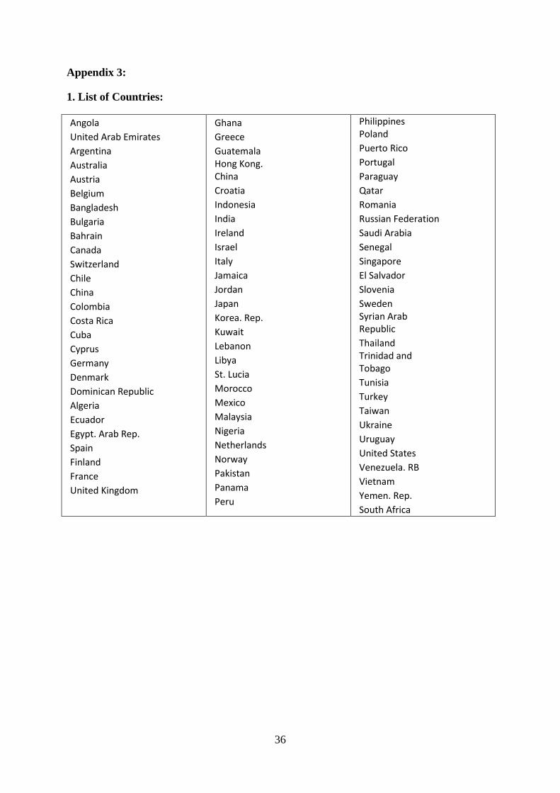
36

Appendix 3:

1. List of Countries:

Angola United Arab Emirates Argentina Australia Austria Belgium Bangladesh Bulgaria Bahrain

Canada Switzerland Chile China Colombia Costa Rica Cuba Cyprus Germany Denmark Dominican Republic Algeria

Ecuador Egypt. Arab Rep. Spain Finland France United Kingdom

Ghana Greece Guatemala Hong Kong. China Croatia Indonesia India Ireland

Israel Italy Jamaica Jordan Japan Korea. Rep. Kuwait Lebanon Libya St. Lucia Morocco Mexico

Malaysia Nigeria Netherlands Norway Pakistan Panama Peru

Philippines Poland Puerto Rico Portugal Paraguay Qatar Romania Russian Federation Saudi Arabia

Senegal Singapore El Salvador Slovenia Sweden Syrian Arab Republic Thailand Trinidad and Tobago Tunisia Turkey

Taiwan Ukraine Uruguay United States Venezuela. RB Vietnam Yemen. Rep. South Africa

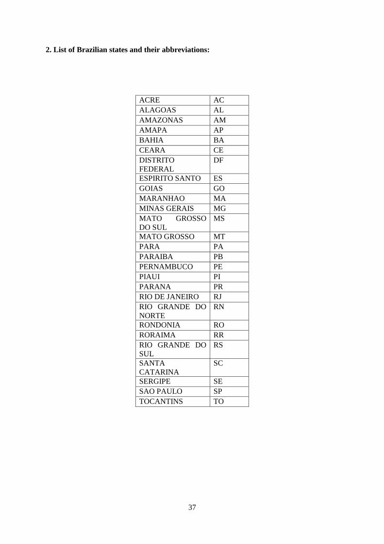
37

2. List of Brazilian states and their abbreviations:

ACRE AC

ALAGOAS AL

AMAZONAS AM

AMAPA AP

BAHIA BA

CEARA CE

DISTRITO

FEDERAL

DF

ESPIRITO SANTO ES

GOIAS GO

MARANHAO MA

MINAS GERAIS MG

MATO GROSSO

DO SUL

MS

MATO GROSSO MT

PARA PA

PARAIBA PB

PERNAMBUCO PE

PIAUI PI

PARANA PR

RIO DE JANEIRO RJ

RIO GRANDE DO

NORTE

RN

RONDONIA RO

RORAIMA RR

RIO GRANDE DO

SUL

RS

SANTA

CATARINA

SC

SERGIPE SE

SAO PAULO SP

TOCANTINS TO