MPRAMunich Personal RePEc Archive

The relative effectiveness of Monetaryand Fiscal Policies on growth: what doeslong-run SVAR model tell us?

Huseyin Sen and Ayse Kaya

Yıldırım Beyazıt University, Izmir Katip Celebi University, Turkey

31. July 2015

Online at http://mpra.ub.uni-muenchen.de/65903/MPRA Paper No. 65903, posted 4. August 2015 09:22 UTC

The Relative Effectiveness of Monetary and Fiscal Policies on Growth:

What Does Long-run SVAR Model Tell Us?*

This Version: July 31, 2015

Abstract

This paper studies empirically the relative effectiveness of monetary and fiscal policies on growth.

Unlike many previous papers which have focused, to a large extent, on the effect of monetary or

fiscal policies separately, this paper considers the comparative efficacy of the two policies on

growth by applying the Structural Vector Autoregression (SVAR) model to the quarterly data for

Turkey over the period 2001:Q1-2014:Q2. The empirical findings of this paper show that both

monetary and fiscal policies do have significant effects on growth. However, monetary policy is

more effective than fiscal policy in stimulating growth. More specifically, interest rate ―a

monetary policy variable― is the most potent instrument in affecting growth. Then budget deficit

―a fiscal policy variable― becomes the second important variable after interest rate. These

findings suggest that although the relative effectiveness in boosting growth is different, both

policies significantly influence growth, suggesting that they should be used jointly but in an

efficient manner.

Key Words : Monetary Policy, Fiscal Policy, Growth, Macroeconomic Policy Management,

SVAR, Turkey.

JEL Code : E52, E58, E62, E63

1. Introduction

Undoubtedly, macroeconomic policy plays a fundamental role in providing as well as maintaining

sustainable and acceptable economic environment which makes it possible for an economy to

achieve a faster, stable and sustainable growth. This fundamental role is conducted by the two

leading instruments of macroeconomic policy in an economy: Monetary and fiscal policies.

However, the comparative efficacy of both monetary and fiscal policies is highly an unresolved

issue between the Keynesians and Monetarists especially since 1960s. In this regard, theoretical as

well as empirical debates are still on-going. The Keynesians strongly argue that fiscal policy is

more effective in relation to monetary policy in stimulating economic activity, while the

Monetarists assert the opposite, claiming that this is the case with monetary policy. This dispute

between two main economic views has never resolved and has been still on-going among

academic economists as well as policymakers. The seminal paper by Andersen and Jordon (1968)

sparked empirical discussions on the relative effectiveness of the two policies on economic

activity. In reviewing the literature, to date no convincing empirical evidence has been found with

regard to the relative effectiveness of monetary and fiscal policies.

The recent two developments, the Stability and Growth Pact of the EU and then more recent

global recession broke out in the aftermath of the 2008 financial crisis, have received a renewed

attention on the comparative efficacy of monetary and fiscal policies.

* We are grateful to Barış Alparslan for helpful comments and suggestions.

The primary purpose of this paper is to empirically examine which of monetary and fiscal policies

is more effective in stimulating growth. The paper attempts to answer the following questions: i)

if monetary and fiscal policies are the primary instruments of macroeconomic policy and

closely related to each other in achieving desirable macroeconomic outcomes, and then what is

their relative effectiveness in terms of growth ? ; ii) how and what direction growth can respond

to changes in these policies ?; iii) are they substitute or competent to each other ?

We strongly believe that to answer all these questions properly, the econometrical model chosen

is highly important. Generally speaking, the SVAR model proposed by Blanchard and Perotti

(2002) and then developed further by Perotti (2005) is a most suitable model in capturing the

relative effectiveness of monetary and fiscal policies. The first and foremost advantage of the

SVAR model is its simplicity. Secondly, it is a well-suited tool, such as impulse response

functions and variance decomposition, for tracing the dynamic interactions between a set of

endogenous variables (Petrevski et al., 2015). Thirdly, to the best of our knowledge, to date it has

not been employed for examining the relative effectiveness of monetary and fiscal policies (See

Appendix).

The rest of the paper is designed as follows: Section 2 provides an overview with regard to

monetary and fiscal policy stance in Turkey, while Section 3 reviews the related empirical

studies. Section 4 then outlines the data and methodology of this paper. Section 5 reports and

discusses the empirical findings. And finally, a conclusion is presented in Section 6.

2. An Overview of Monetary and Fiscal Policy Stance in Turkey

Monetary and fiscal policy is an interesting as well as important issue not only for developed

countries but also for developing ones. Turkey is also the case in this matter. Before turning our

attention to empirical analysis, it would therefore be useful to review recent developments in the

Turkish economy with a special focus on monetary and fiscal policy.

Turkey experienced with high and chronic inflation starting from the second half of 1970s and

CPI inflation reached triple digits in 1980 and 1994 soon after the introduction of two major

stabilization programmes. As a result of these programmes, Turkey was kept away from

hyperinflation trap along with other economic difficulties. Nevertheless throughout the 1980s and

1990s inflation remained high and chronic, exceeding the levels of 60% on average. Undoubtedly,

the main reason behind high and chronic inflation was unsustainable budget deficits. Budget

deficits were largely and often financed through the Central Bank of the Republic of Turkey’s

[CBRT] resources especially from the 1970s to 1984. It would not be wrong to say that the

CBRT operated like a branch of the Treasury in that period. Under the law of the CBRT, the

Central Bank used to lend short-term advances to the Treasury at the beginning of every fiscal

year as much as 15% of current year’s public allowances. In fact these advances were never

returned or paid back by the Treasury in time. Within that period, short-term advances to the

Treasury turned to a cumulative debt, an unpaid domestic debt of the treasury. After the year

1984, the Treasury changed its deficit financing policy by switching from monetization to

domestic debt borrowing due to a fear of the possibility of accelerating inflation trap. However,

this policy change made the economic situation worse. The Turkish economy, at that time,

faced with a significant decline in GDP, while inflation continued to remain high and chronic

during the second half of the 1980s and throughout the 1990s. All these developments forced

the Treasury and CBRT officials to make a good deal to overcome the adverse economic

situation. And then they decided to make a protocol for providing monetary and fiscal policy

coordination. The protocol came under implementation in the year 1997.

Under the protocol, the treasury would no longer demand for short-term advances from the

CBRT. Soon after the implementation of the protocol, all the loans provided by the CBRT not

only to the Treasury, but also to other public institutions, such as state economic enterprises and

municipalities, were cut down. Shortly after the implementation of the protocol the economy

has made a quite good progress. However, Turkey was hit by twin consecutive economic crises,

November-2000 and February-2001, due to a number of economic and/or political reasons. In

fact, these successive crises were a turning point for the Turkish economy. Immediately after all

the articles of the CBRT which ruled on financing governmental organisation were repealed, it

became formally independent monetary institution. Besides, a series of structural reforms,

ranging from a more robust public finance management to prudential measures which

strengthened the financial sector were put into practice. These measures showed their impact

shortly. Soon after the central bank became independent and structural reforms were introduced,

inflation started to drop sharply seeing historically a low level along with significant reductions

in interest rates and other macroeconomic indicators.

Overall, in the second half of the1980s and 1990s the Turkish economy like many other

developing economies was characterised with a fragile banking sector, a non-independent central

bank, a poor fiscal policy management, and a double-headed economic management. All these

resulted in a bad economic environment, thereby leading to extremely high interest rates, high

and chronic inflation, huge budget deficits, unstable exchange rate, unequal income distribution,

low investment and high unemployment, and so on. Since 2002, the Turkish economy has made

a significant progress from a number of aspects. Long lasting inflation incredibly dropped to

single digits, growth rate made a remarkable high progress; for instance, it was annually on

average at 7% between the years 2002-2007. All these put Turkey in a better place among

emerging economies. However, the Turkish economy has recently had high current account

deficits, exceeding much more than the Dornbush threshold, along with high unemployment

and slowing growth. Since then, like many other countries regardless of whether industrialized

or developing one, Turkey has showed economically a poor performance. Annual growth rate

dropped from 9.2% in 2010 to 2.9% in 2014 as CPI remained relatively high levels. In addition

to these, between the years 2010-2014, current account deficit-to-GDP always remained above

the Dornbush threshold, which is thought to be financial crisis indicator. The last five year’s

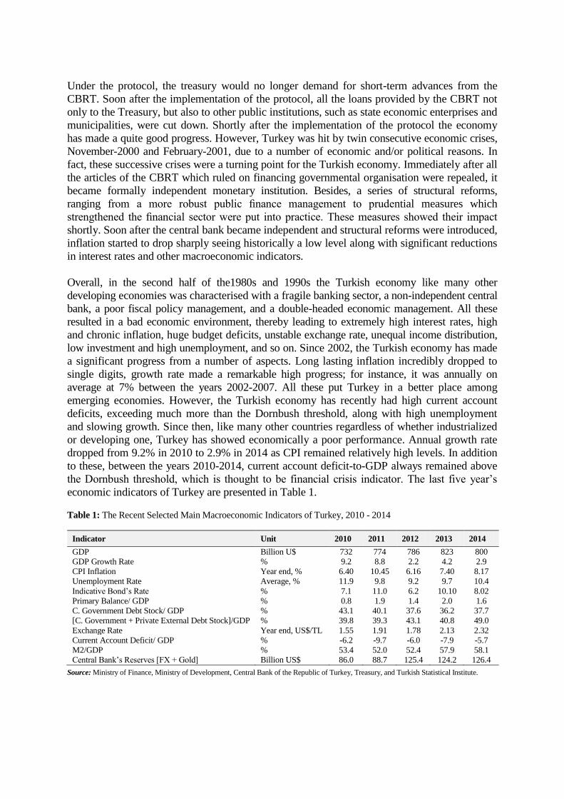
economic indicators of Turkey are presented in Table 1.

Table 1: The Recent Selected Main Macroeconomic Indicators of Turkey, 2010 - 2014

Indicator Unit 2010 2011 2012 2013 2014

GDP Billion U$ 732 774 786 823 800

GDP Growth Rate % 9.2 8.8 2.2 4.2 2.9

CPI Inflation Year end, % 6.40 10.45 6.16 7.40 8.17

Unemployment Rate Average, % 11.9 9.8 9.2 9.7 10.4

Indicative Bond’s Rate % 7.1 11.0 6.2 10.10 8.02

Primary Balance/ GDP % 0.8 1.9 1.4 2.0 1.6

C. Government Debt Stock/ GDP % 43.1 40.1 37.6 36.2 37.7

[C. Government + Private External Debt Stock]/GDP % 39.8 39.3 43.1 40.8 49.0

Exchange Rate Year end, US$/TL 1.55 1.91 1.78 2.13 2.32

Current Account Deficit/ GDP % -6.2 -9.7 -6.0 -7.9 -5.7

M2/GDP

Central Bank’s Reserves [FX + Gold]

%

Billion US$

53.4

86.0

52.0

88.7

52.4

125.4

57.9

124.2

58.1

126.4

Source: Ministry of Finance, Ministry of Development, Central Bank of the Republic of Turkey, Treasury, and Turkish Statistical Institute.

3. Related Empirical Studies

As mentioned earlier, empirical discussions related to the relative effectiveness of monetary and

fiscal policies date back to the 1960s. In this regard, the two seminal papers by Friedman and

Meiselman (1963), and Andersen and Jordan (1968) are important examples of this case.

Especially, the paper by Andersen and Jordan (1968) is thought of as the first empirical study

on the relative effectiveness of monetary and fiscal policy on output (See, for instance, Waud

(1974), and Hussain (2014) for a detailed discussion). In examining the relative effectiveness of

monetary and fiscal policies, Andersen and Jordan (1968) employed a dynamic econometric

model and concluded that monetary policy is more certain, more effective and faster in

influencing the economy in relation to fiscal policy. Since then, the relative effectiveness of

monetary and fiscal policies has become the subject of numerous empirical studies. By the late

1980s, however, many studies agreed upon the superiority of monetary policy over fiscal policy

in terms of magnitude, predictability, and lag of influence at least in the case of the US

(Atchariyachanvanich, 2007).

In line with the purpose of this paper, in this section we will only concentrate on the empirical

studies. The current literature contains many studies which have highlighted the effects of

monetary and fiscal policies on growth and it has been continuing to expand. Especially, in last

two or three decades, the number of studies examining the effect of fiscal policy compared to

that of monetary policy has increased further. This may be attributed to the increasing role of

fiscal policy in combatting economic turbulences and downturns which were faced by a number

of both developed and developing countries.

In reviewing the literature, we observe that earlier studies as to the effectiveness of monetary

and fiscal policies have focused to large extent on industrialized countries, especially on the US.

For example, an early study by Waud (1974) investigated the relative efficacy of monetary

policy vis-à-vis fiscal policy on GNP in the US and found that the influence of both policies on

economic activity is significant and appears equally important. These results are in sharp

contrast to those of Andersen and Jordan (1968), arguing that monetary influences on economic

activity are much stronger than fiscal ones.

Another study by Batten and Hafer (1983) examined the relative effectiveness of monetary and

fiscal actions in six industrialized countries covering the UK, the US, Canada, France and

Germany for the period of the late 1960s – the early 1980s by employing the St. Louis approach.

They concluded that while monetary actions have a significant as well as permanent effect on

nominal GNP growth, fiscal actions exert no statistically significant and lasting influence. A

recent study on the US by Senbet (2011) investigated the relative effectiveness of the two

policies and reached that monetary policy affects the real output relatively better than fiscal

policy.

In recent years we also observe a considerable increase in the studies which have examined the

topic in the context of developing countries. These sorts of studies range from low-income

developing countries to relatively high income countries. For instance, the studies of Ajisafe

and Folorunso (2002), Olaloye and Ikhide (1995), Adefeso and Mobolaji (2010), among some

others, centered on the case of Nigeria, other studies such as Chowdhury (1986a, 1986b), Looney

(1989), Fatima and Iqbal (2003), Ali and Ahmad (2010), Havi and Enu (2014), focused on the

other countries like Bangladesh, Korea, Saudi Arabia, Pakistan, Serbia, Ghana, and Kenya (See

Appendix).

Using cointegration and error correction estimation techniques, a country-specific study by

Ajisafe and Folorunso (2002) examined the relative efficacy of monetary and fiscal policy in

Nigeria during the period 1970-1998, and found that monetary policy rather than fiscal policy

exerts a great impact on economic activity. Another study by Adefeso and Mobolaji (2010) on

the same country but for a different time period, 1970-2007, applied the same econometric

procedure and then reached the same results as those found by Ajisafe and Folorunso (2002),

suggesting that the effectiveness of monetary policy is much stronger than that of fiscal policy.

However, in contrast to the two studies above, a study by Olaloye and Ikhide (1995) revealed

that fiscal policy exerts more influence on the economy than monetary policy. In addition to

these contradictory empirical findings, a recent study on the same country by Sanni et al. (2012)

produces further controversy over the issue. Their findings imply that the relative efficiency of

the two policies is different from each other, depending on the number as well as the type of

variables. Accordingly, monetary policy exerts more influence on the economy when all the

five variables ―debt financed deficits, fiscal deficit ratio, money printing financed deficits, M1,

and M2 ― are taken into account.1 However, the exclusion of money printing financed deficits

reverses the case. Based on all these findings, they argued that none of the policies is superior to

the other, and that a proper mix of both monetary and fiscal policies may spur economic

growth.

Another recent country-specific study by Havi and Enu (2014) examined the relative

importance of monetary and fiscal policy on growth in Ghana by using OLS estimation

techniques for the period 1980-2012. Their study showed that although the effect of monetary

policy is more powerful, both policies positively affect growth in the case of Ghana. In a similar

vein, another country-specific study by Jawaid et al. (2010) analyzed the comparative effect of

the two potent macroeconomic policy tools on growth in Pakistan during the period 1981-2009.

Their empirical findings revealed that there exists a positive long-run relationship between both

policies and growth. However, according to their findings, monetary policy is more effective

than fiscal policy in promoting growth. In contrast, the study of Mahmood and Sial (2011) using

time series data over the period 1973-2008 for the same country found that monetary and fiscal

policies both play a significant role in growth in Pakistan.

In recent years, we have also observed from the literature that the number of studies examining

the relative effectiveness of monetary and fiscal policies on the basis of country regardless of

their development level rather than single country has increased. Among these sorts of studies,

the studies such as Batten and Hafer (1983), Owoye and Onafowora (1994), Jayaraman (2002),

Atchariyachanvanich (2007), Ali et al. (2008), Hussain (2014), and Petrevski et al. (2015) are

the main studies. For instance, Owoye and Onafowora (1994) examined the relative importance

of monetary and fiscal policies in stimulating growth in 10 African countries Burundi,

Ethiopia, Ghana, Kenya, Morocco, Nigeria, Sierra Leone, South Africa, Tanzania and Zambia

by using a Trivariate Vector Autoregressive (VAR) model for the annual data spanning from

1960 to 1990. Their findings support the Monetarist view in 5 of 10 countries, indicating that

monetary policy is more important than fiscal policy. However, for the rest of 5 countries, their

findings showed that Keynesian view, which is that fiscal policy is more important than

monetary policy, was confirmed. Based on these findings, they argued that it is not possible to

generalize a particular economic philosophy ―neither the monetarist, nor the Keynesian

view― for African countries with regard to the relative importance of monetary and fiscal

policies.

1 The first three is the proxies for fiscal policy, whereas the latter two is the proxies for monetary policy.

A highly interesting study by Atchariyachanvanich (2007) investigated the relative efficacy of

monetary policy vis-à-vis fiscal policy on the output level of 12 countries; some of them are

industrialized countries, while the others developing countries. Employing OLS technique to the

quarterly data ranging from the early 1990s to the late 2004, and then dividing the twelve

countries into three main groups as: i) monetary policy dominated, ii) fiscal policy dominated,

iii) monetary and fiscal policies mixed countries, he examined the impact of the two policies on

the output level. His study showed that the impact of the two policies is not clearly

distinguishable. Another, but a fresh, multiple-country study by Petrevski et al. (2015) examined

the effects of monetary and fiscal policies in three South Eastern Europe economies: Bulgaria,

Croatia, and Macedonia. Applying the recursive VARs to the quarterly data for 1999-2011, they

found that positive fiscal shocks induce higher output in the all economies, pointing to the

expansionary effects of fiscal consolidation.

Overall, in reviewing the related literature we can conclude that although there exist the

vast majority of studies examining the relative effectiveness of monetary and fiscal

policies, the empirical findings of these studies are highly mixed. In other words, the

empirical studies reveal inconclusive results with regard to the relative effectiveness of

two potent macroeconomic policy tools. Some studies, such as Kretzmer (1992), Ali et al.

(2008), Adesefo (2010), Senbet (2011), Rakic and Radenic (2013), Havi and Enu (2014),

found that monetary policy is more effective in boosting growth compared to fiscal policy,

whereas some others, i.e. Chowdury (1986), Olaloye and Ikhide (1995), found the opposite

results. On the other hand, other studies, such as Batten and Hafer (1983), Rahman (2009),

and Anna (2012), suggest that only monetary policy is effective but fiscal policy is

ineffective, whereas some other studies ―Chowdhury (1986a), Olaloye and Ikhide (1995),

and Cyrus and Elias (2014), claim the opposite results. Moreover, multiple-country studies

yield highly mixed results. For instance, in some countries monetary policy is dominant to

fiscal policy or vice versa, while in others the results is inconclusive (See, Appendix).

These results do not allow us to make a generalization with regard to the relative

effectiveness of monetary and fiscal policies. The contradictory empirical results which

emerged from the studies above may be attributed to a number of factors, depending on

country-specific elements such as institutional, developmental, political and so on as well as

methodological approaches, variables chosen, treatment, etc.

4. Data and Methodology

In this section, we first present the data. And then, we produce impulse-response functions. As a

next step, we forecast error variance decomposition analysis from the estimated SVAR model.

4.1. Data

In this paper, we use the quarterly data for Turkey covering the period 2001:Q1-2014:Q2. The

data is compelled from main national resources, such as the Central Bank of the Republic of

Turkey, the Ministry of Finance, and the Ministry of Development. The data set is presented in

Table 2.

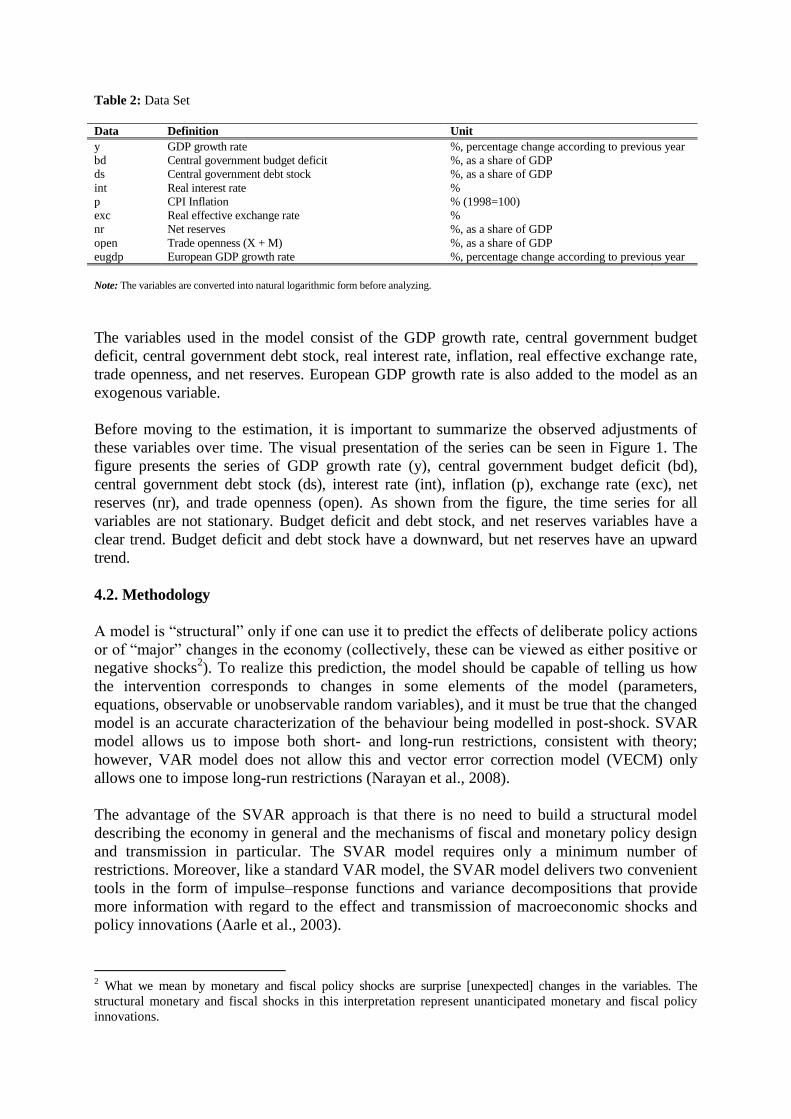
Table 2: Data Set

Data Definition Unit

y GDP growth rate %, percentage change according to previous year

bd Central government budget deficit %, as a share of GDP

ds Central government debt stock %, as a share of GDP

int Real interest rate %

p CPI Inflation % (1998=100)

exc Real effective exchange rate %

nr Net reserves %, as a share of GDP

open Trade openness (X + M) %, as a share of GDP

eugdp European GDP growth rate %, percentage change according to previous year

Note: The variables are converted into natural logarithmic form before analyzing.

The variables used in the model consist of the GDP growth rate, central government budget

deficit, central government debt stock, real interest rate, inflation, real effective exchange rate,

trade openness, and net reserves. European GDP growth rate is also added to the model as an

exogenous variable.

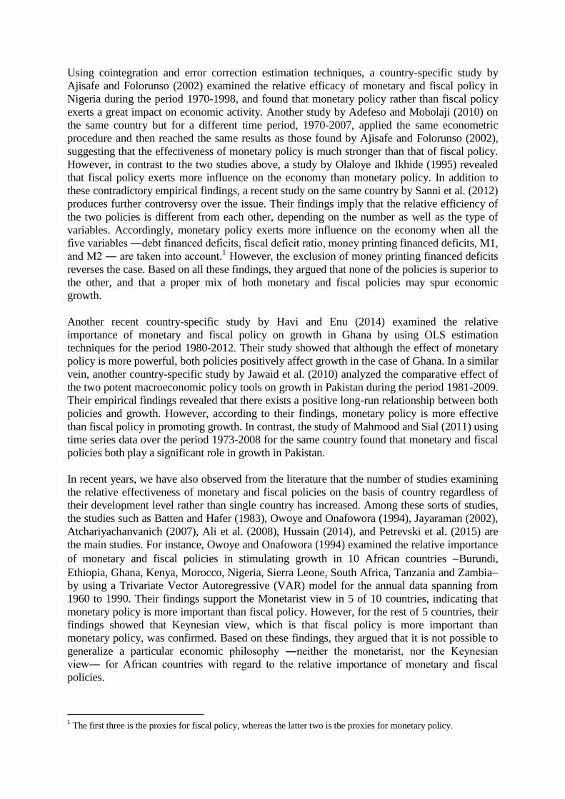
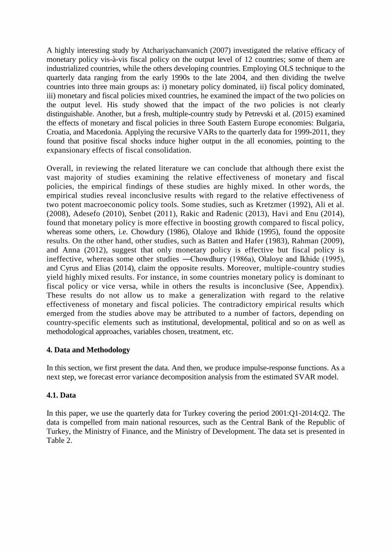
Before moving to the estimation, it is important to summarize the observed adjustments of

these variables over time. The visual presentation of the series can be seen in Figure 1. The

figure presents the series of GDP growth rate (y), central government budget deficit (bd),

central government debt stock (ds), interest rate (int), inflation (p), exchange rate (exc), net

reserves (nr), and trade openness (open). As shown from the figure, the time series for all

variables are not stationary. Budget deficit and debt stock, and net reserves variables have a

clear trend. Budget deficit and debt stock have a downward, but net reserves have an upward

trend.

4.2. Methodology

A model is “structural” only if one can use it to predict the effects of deliberate policy actions

or of “major” changes in the economy (collectively, these can be viewed as either positive or

negative shocks2). To realize this prediction, the model should be capable of telling us how

the intervention corresponds to changes in some elements of the model (parameters,

equations, observable or unobservable random variables), and it must be true that the changed

model is an accurate characterization of the behaviour being modelled in post-shock. SVAR

model allows us to impose both short- and long-run restrictions, consistent with theory;

however, VAR model does not allow this and vector error correction model (VECM) only

allows one to impose long-run restrictions (Narayan et al., 2008).

The advantage of the SVAR approach is that there is no need to build a structural model

describing the economy in general and the mechanisms of fiscal and monetary policy design

and transmission in particular. The SVAR model requires only a minimum number of

restrictions. Moreover, like a standard VAR model, the SVAR model delivers two convenient

tools in the form of impulse–response functions and variance decompositions that provide

more information with regard to the effect and transmission of macroeconomic shocks and

policy innovations (Aarle et al., 2003).

2 What we mean by monetary and fiscal policy shocks are surprise [unexpected] changes in the variables. The

structural monetary and fiscal shocks in this interpretation represent unanticipated monetary and fiscal policy

innovations.

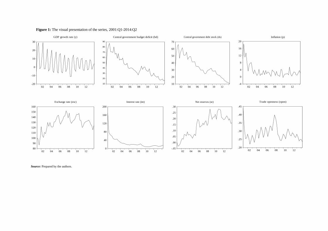
Figure 1: The visual presentation of the series, 2001:Q1-2014:Q2

Source: Prepared by the authors.

-20

-10

0

10

20

30

02 04 06 08 10 12

GDP growth rate (y)

10

20

30

40

50

60

70

80

90

02 04 06 08 10 12

Central government budget deficit (bd)

10

20

30

40

50

60

70

02 04 06 08 10 12

Central government debt stock (ds)

-4

0

4

8

12

16

20

02 04 06 08 10 12

Inflation (p)

80

90

100

110

120

130

140

150

160

02 04 06 08 10 12

Exchange rate (exc)

0

40

80

120

160

200

02 04 06 08 10 12

Interest rate (int)

-.05

.00

.05

.10

.15

.20

.25

.30

02 04 06 08 10 12

Net reserves (nr)

.20

.25

.30

.35

.40

.45

02 04 06 08 10 12

Trade openness (open)

The structural VAR model imposes identifying restrictions upon VAR estimates to recover

structural innovations from the estimated VAR. The identification can be practically achieved

through imposing identifying short- or long-run restrictions. The advantage of using long-run

restrictions is that in a number of cases, economic theory provides more guidance about long-

run relationships than about short-run dynamics. Short-run restrictions impose typically that

the effect of a given shock to a certain variable is null, which can be achieved by setting the

appropriate elements in C(0) to zero. As to long-run restrictions, they impose typically that

there is no long-run effect of a shock to a variable, which is achieved by setting the

appropriate elements of C(1) to zero. In order to identify exactly a VAR model of n

endogenous variables, (n2−n)/2 restrictions need to be imposed in the structural model (Aarle

et al., 2003).

We can begin with a reduced form VAR model of the following form (Narayan et al., 2008):

= + … + + + + [1]

Where p stands for the order of the VAR model, Y stands for an nx1 vector of endogenous

variables, stands for an nx1 vector of reduced form residuals, respectively. We can safely

ignore the deterministic component simply because it is unaffected by shocks to the system.

Then the SVAR model can be typed as follows:

= + … +

+ B [2]

The matrix A is used to model the instantaneous relationships, while the matrix B contains

structural form parameters of the model. is an nx1 vector of structural disturbances and

VAR ( ) = ʌ, where ʌ is a diagonal matrix with the variance of structural disturbances

making up the diagonal elements.

It is commonly accepted view in the literature that shocks cannot be observed, directly. There

is, therefore, a need to impose some restrictions. For this, the common practice is to multiply

Eq. (2) by leading to the following relationship between the reduced form disturbances

and the structural disturbances:

= [3]

This allows us to rewrite Eq. [3] as follows:

A = [4]

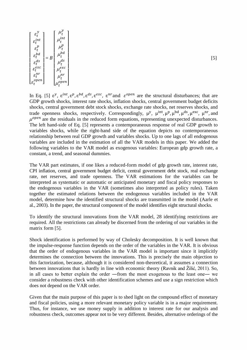
Our SVAR model encompasses eight variables consisting of GDP growth rate (y), interest rate

(int), inflation (p), central government budget deficit (bd), central government debt stock (ds),

exchange rate (exc), reserves (nr), and trade openness (open). Therefore, we consider structural

VAR model with the following restrictions:

[

]

=

[

]

[5]

In Eq. [5] , are the structural disturbances; that are

GDP growth shocks, interest rate shocks, inflation shocks, central government budget deficits

shocks, central government debt stock shocks, exchange rate shocks, net reserves shocks, and

trade openness shocks, respectively. Correspondingly, , and

are the residuals in the reduced form equations, representing unexpected disturbances.

The left hand-side of Eq. [5] represents a contemporaneous response of real GDP growth to

variables shocks, while the right-hand side of the equation depicts no contemporaneous

relationship between real GDP growth and variables shocks. Up to one lags of all endogenous

variables are included in the estimation of all the VAR models in this paper. We added the

following variables to the VAR model as exogenous variables: European gdp growth rate, a

constant, a trend, and seasonal dummies.

The VAR part estimates, if one likes a reduced-form model of gdp growth rate, interest rate,

CPI inflation, central government budget deficit, central government debt stock, real exchange

rate, net reserves, and trade openness. The VAR estimations for the variables can be

interpreted as systematic or automatic or anticipated monetary and fiscal policy responses to

the endogenous variables in the VAR (sometimes also interpreted as policy rules). Taken

together the estimated relations between the endogenous variables included in the VAR

model, determine how the identified structural shocks are transmitted in the model (Aarle et

al., 2003). In the paper, the structural component of the model identifies eight structural shocks.

To identify the structural innovations from the VAR model, 28 identifying restrictions are

required. All the restrictions can already be discerned from the ordering of our variables in the

matrix form [5].

Shock identification is performed by way of Cholesky decomposition. It is well known that

the impulse-response function depends on the order of the variables in the VAR. It is obvious

that the order of endogenous variables in the VAR model is important since it implicitly

determines the connection between the innovations. This is precisely the main objection to

this factorization, because, although it is considered non-theoretical, it assumes a connection

between innovations that is hardly in line with economic theory (Ravnik and Žilić, 2011). So,

in all cases to better explain the order ―from the most exogenous to the least one― we

consider a robustness check with other identification schemes and use a sign restriction which

does not depend on the VAR order.

Given that the main purpose of this paper is to shed light on the compound effect of monetary

and fiscal policies, using a more relevant monetary policy variable is in a major requirement.

Thus, for instance, we use money supply in addition to interest rate for our analysis and

robustness check, outcomes appear not to be very different. Besides, alternative orderings of the

variables implies less attractive identifying restrictions. We experimented with alternative

identifying restrictions and generally found that the results not overly sensitive to small changes

in the identifying restrictions.

5. Empirical Findings

Before proceeding to the estimation of our model, we need to test whether the variables under

consideration are stationary. Recalling that in order to carry out a VAR analysis, time series

must be stationary. For this purpose, we first applied Augmented Dickey-Fuller (ADF) test.

The test results were reported in Table 3. As shown from the table, all variables are I(1). Here,

the null hypothesis is that the series have unit root, which indicates non-stationarity or vice

versa. In other words, the first differences of the y, int, p, bd, ds, exc, nr, and open are

stationary, implying that these variables are in fact integrated of order one I(1).

Table 3: Augmented Dickey-Fuller (ADF) Test Results, 2001:Q1-2014:Q2

Series First Difference

Constant

Critical Value

(% 1)

y -5.1734 (1)* -3.5777

int -4.7321 (1)* -3.5713

p -3.6545 (1)* -3.5924

bd -4.6280 (1)* -3.5713

ds -2.6609 (1)* -2.5992

exc -4.2061 (1)* -3.5777

nr -6.1840 (1)* -3.5654

open -4.3265(1)* -3.5777

Note: The numbers in parentheses indicate the selected lag order of the ADF models. Lags chosen are based upon Akaike Information

Criterion (AIC). The critical values are obtained from MacKinnon (1991) for the ADF test. The ADF tests examine the null hypothesis of a

unit root against the stationary alternative. Asterisks (*) denote statistical significance at 5 % and variables have constant and linear trend, respectively.

Source: Computed by the authors.

And then, we identified the order of the VAR model using the Akaike Information Criterion

(AIC), Schwarz Information Criteria (SC), and Hannan-Quinn Information Criteria (HQ). They

all suggest a VAR model of order one. The optimal lag length criteria were presented in Table

4. After obtaining the estimation results of the VAR model, we implemented an AR Roots test

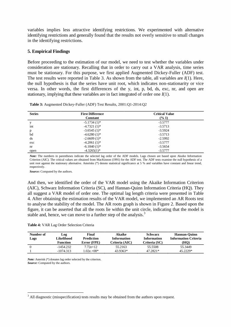
to analyse the stability of the model. The AR roots graph is shown in Figure 2. Based upon the

figure, it can be asserted that all the roots lie within the unit circle, indicating that the model is

stable and, hence, we can move to a further step of the analysis.3

Table 4: VAR Lag Order Selection Criteria

Number of

Lags

Log

Likelihood

Function

Final

Prediction

Error (FPE)

Akaike

Information

Criteria (AIC)

Schwarz

Information

Criteria (SC)

Hannan-Quinn

Information Criteria

(HQ)

0 -1454.232 7.72e+12 55.2163 55.5508 55.3449

1 -1074.313 1.02e.+08* 43.9363* 47.2821* 45.2229*

Note: Asterisk (*) donates lag order selected by the criterion.

Source: Computed by the authors.

3 All diagnostic (misspecification) tests results may be obtained from the authors upon request.

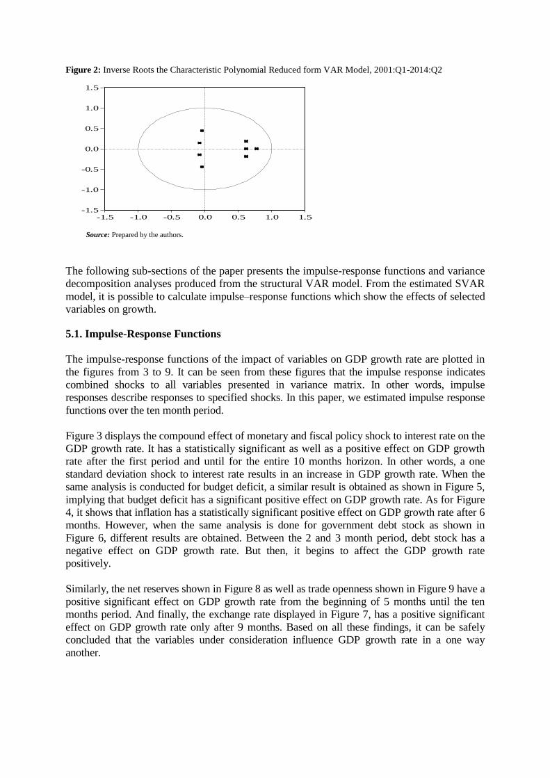
Figure 2: Inverse Roots the Characteristic Polynomial Reduced form VAR Model, 2001:Q1-2014:Q2

Source: Prepared by the authors.

The following sub-sections of the paper presents the impulse-response functions and variance

decomposition analyses produced from the structural VAR model. From the estimated SVAR

model, it is possible to calculate impulse–response functions which show the effects of selected

variables on growth.

5.1. Impulse-Response Functions

The impulse-response functions of the impact of variables on GDP growth rate are plotted in

the figures from 3 to 9. It can be seen from these figures that the impulse response indicates

combined shocks to all variables presented in variance matrix. In other words, impulse

responses describe responses to specified shocks. In this paper, we estimated impulse response

functions over the ten month period.

Figure 3 displays the compound effect of monetary and fiscal policy shock to interest rate on the

GDP growth rate. It has a statistically significant as well as a positive effect on GDP growth

rate after the first period and until for the entire 10 months horizon. In other words, a one

standard deviation shock to interest rate results in an increase in GDP growth rate. When the

same analysis is conducted for budget deficit, a similar result is obtained as shown in Figure 5,

implying that budget deficit has a significant positive effect on GDP growth rate. As for Figure

4, it shows that inflation has a statistically significant positive effect on GDP growth rate after 6

months. However, when the same analysis is done for government debt stock as shown in

Figure 6, different results are obtained. Between the 2 and 3 month period, debt stock has a

negative effect on GDP growth rate. But then, it begins to affect the GDP growth rate

positively.

Similarly, the net reserves shown in Figure 8 as well as trade openness shown in Figure 9 have a

positive significant effect on GDP growth rate from the beginning of 5 months until the ten

months period. And finally, the exchange rate displayed in Figure 7, has a positive significant

effect on GDP growth rate only after 9 months. Based on all these findings, it can be safely

concluded that the variables under consideration influence GDP growth rate in a one way

another.

-1.5

-1.0

-0.5

0.0

0.5

1.0

1.5

-1.5 -1.0 -0.5 0.0 0.5 1.0 1.5

5.2. Variance Decomposition

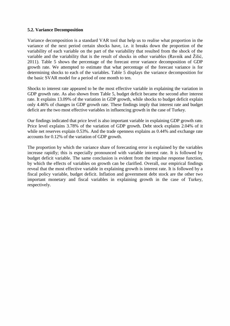
Variance decomposition is a standard VAR tool that help us to realise what proportion in the

variance of the next period certain shocks have, i.e. it breaks down the proportion of the

variability of each variable on the part of the variability that resulted from the shock of the

variable and the variability that is the result of shocks in other variables (Ravnik and Žilić,

2011). Table 5 shows the percentage of the forecast error variance decomposition of GDP

growth rate. We attempted to estimate that what percentage of the forecast variance is for

determining shocks to each of the variables. Table 5 displays the variance decomposition for

the basic SVAR model for a period of one month to ten.

Shocks to interest rate appeared to be the most effective variable in explaining the variation in

GDP growth rate. As also shown from Table 5, budget deficit became the second after interest

rate. It explains 13.09% of the variation in GDP growth, while shocks to budget deficit explain

only 4.46% of changes in GDP growth rate. These findings imply that interest rate and budget

deficit are the two most effective variables in influencing growth in the case of Turkey.

Our findings indicated that price level is also important variable in explaining GDP growth rate.

Price level explains 3.78% of the variation of GDP growth. Debt stock explains 2.04% of it

while net reserves explain 0.53%. And the trade openness explains as 0.44% and exchange rate

accounts for 0.12% of the variation of GDP growth.

The proportion by which the variance share of forecasting error is explained by the variables

increase rapidly; this is especially pronounced with variable interest rate. It is followed by

budget deficit variable. The same conclusion is evident from the impulse response function,

by which the effects of variables on growth can be clarified. Overall, our empirical findings

reveal that the most effective variable in explaining growth is interest rate. It is followed by a

fiscal policy variable, budget deficit. Inflation and government debt stock are the other two

important monetary and fiscal variables in explaining growth in the case of Turkey,

respectively.

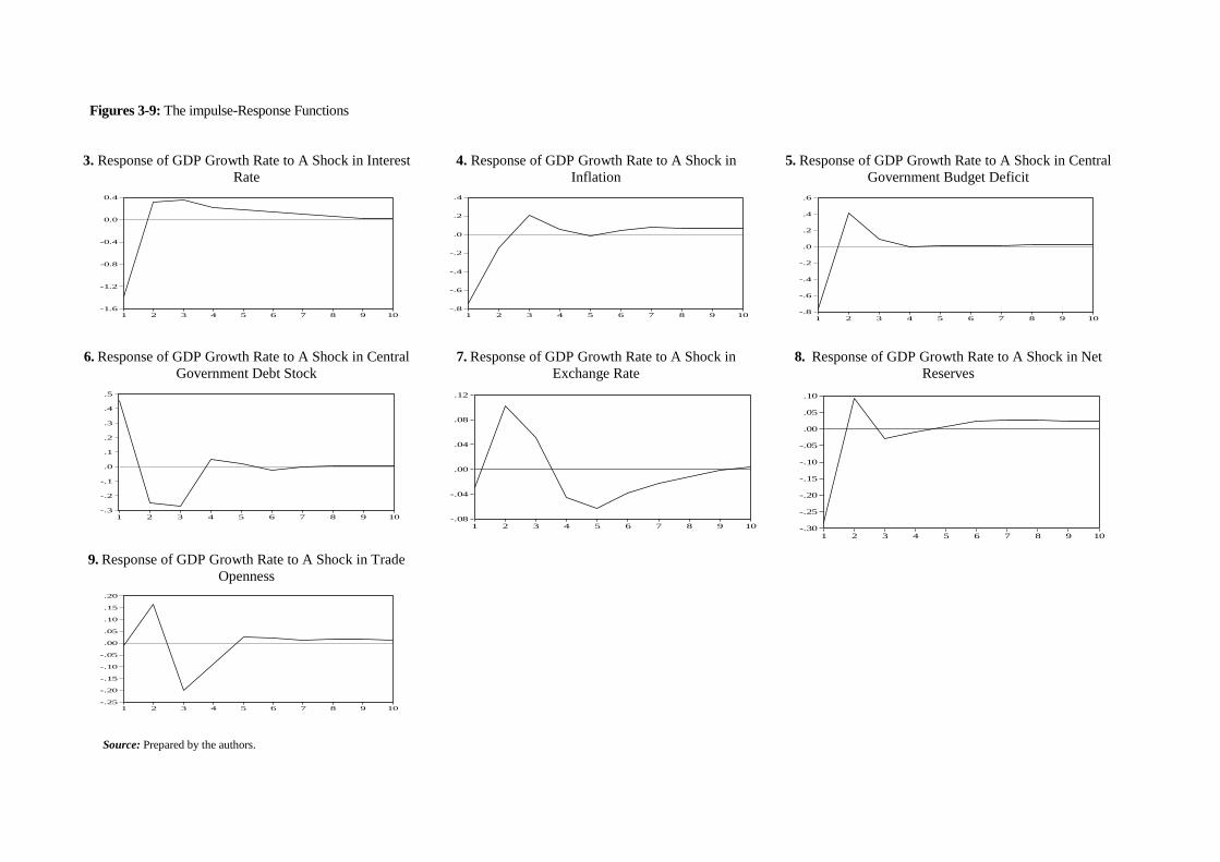
Figures 3-9: The impulse-Response Functions

3. Response of GDP Growth Rate to A Shock in Interest

Rate

4. Response of GDP Growth Rate to A Shock in

Inflation

5. Response of GDP Growth Rate to A Shock in Central

Government Budget Deficit

6. Response of GDP Growth Rate to A Shock in Central

Government Debt Stock

7. Response of GDP Growth Rate to A Shock in

Exchange Rate

8. Response of GDP Growth Rate to A Shock in Net

Reserves

9. Response of GDP Growth Rate to A Shock in Trade

Openness

Source: Prepared by the authors.

-1.6

-1.2

-0.8

-0.4

0.0

0.4

1 2 3 4 5 6 7 8 9 10-.8

-.6

-.4

-.2

.0

.2

.4

1 2 3 4 5 6 7 8 9 10-.8

-.6

-.4

-.2

.0

.2

.4

.6

1 2 3 4 5 6 7 8 9 10

-.3

-.2

-.1

.0

.1

.2

.3

.4

.5

1 2 3 4 5 6 7 8 9 10 -.08

-.04

.00

.04

.08

.12

1 2 3 4 5 6 7 8 9 10 -.30

-.25

-.20

-.15

-.10

-.05

.00

.05

.10

1 2 3 4 5 6 7 8 9 10

-.25

-.20

-.15

-.10

-.05

.00

.05

.10

.15

.20

1 2 3 4 5 6 7 8 9 10

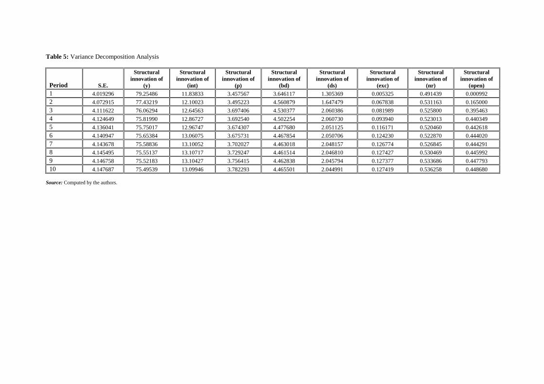
Table 5: Variance Decomposition Analysis

Period S.E.

Structural

innovation of

(y)

Structural

innovation of

(int)

Structural

innovation of

(p)

Structural

innovation of

(bd)

Structural

innovation of

(ds)

Structural

innovation of

(exc)

Structural

innovation of

(nr)

Structural

innovation of

(open)

1 4.019296 79.25486 11.83833 3.457567 3.646117 1.305369 0.005325 0.491439 0.000992

2 4.072915 77.43219 12.10023 3.495223 4.560879 1.647479 0.067838 0.531163 0.165000

3 4.111622 76.06294 12.64563 3.697406 4.530377 2.060386 0.081989 0.525800 0.395463

4 4.124649 75.81990 12.86727 3.692540 4.502254 2.060730 0.093940 0.523013 0.440349

5 4.136041 75.75017 12.96747 3.674307 4.477680 2.051125 0.116171 0.520460 0.442618

6 4.140947 75.65384 13.06075 3.675731 4.467854 2.050706 0.124230 0.522870 0.444020

7 4.143678 75.58836 13.10052 3.702027 4.463018 2.048157 0.126774 0.526845 0.444291

8 4.145495 75.55137 13.10717 3.729247 4.461514 2.046810 0.127427 0.530469 0.445992

9 4.146758 75.52183 13.10427 3.756415 4.462838 2.045794 0.127377 0.533686 0.447793

10 4.147687 75.49539 13.09946 3.782293 4.465501 2.044991 0.127419 0.536258 0.448680

Source: Computed by the authors.

6. Conclusion

In this paper, we examined the relative effectiveness of monetary and fiscal policy shocks on

growth. For this purpose, we applied a long-run SVAR model to the quarterly data for Turkey

for the period 2001:Q1-2014:Q2.

Our findings showed that both monetary and fiscal policies are effective on growth. However,

the relative effectiveness of monetary policy is much stronger than that of fiscal policy. Fiscal

policy for which we used central government deficits and central government debt stock as

proxies accounts for only 6.51% of the changes in GDP growth rate, whereas the rest of the

changes is explained by the monetary policy variables ―interest rate and inflation rate― and

other variables, such as, openness to trade, and real effective exchange rate, which were added

to the our model. However, the magnitudes of the effects of monetary policy variables on growth

are relatively higher compared to fiscal policy variables.

Interest rates which is a proxy variable for monetary policy is the most effective variable. It is

followed by budget deficits variable, which is a proxy for fiscal policy. A shock to interest rate

which is a proxy variable for monetary policy affects GDP growth rate by 13.06 %, whereas

central government deficits, a proxy variable for fiscal policy, influence it by 4.46%. On the

other hand, inflation and government debt stock affect GDP growth rate by 3.78% and 2.04%,

respectively. All these empirical findings indicate that monetary policy is relatively more

effective than fiscal policy in influencing GDP growth rate in Turkey. This implies that

monetary policy is dominant to fiscal policy in the period we examined. Based upon these

findings, it can be argued that i) the effects of monetary and fiscal policies on growth are

different from each other and the effectiveness of the first appears to be much stronger and

larger in all cases, ii) if the two policies are used in a complimentary manner, ceteris paribus, it

is highly likely to obtain a higher GDP growth at least in the case of Turkey.

Our findings are relatively in line with the findings of large number of recent empirical studies,

such as Ali et al. (2008), Havi and Enu (2014), Rakic and Radenovic (2013), Senbet (2011),

Adefeso and Mobolaji (2010), which support the Monetarist view implying that monetary

policy is more effective than fiscal policy in stimulating growth. However, as we noted earlier,

our findings are in sharp contrast to the studies of those, for example, Olaloye and Ikhide

(1995), Rahman (2009), Anna (2012), Cyrus and Elias (2014), suggesting the validity of the

Keynesian view.

Whatever our empirical findings are, however, the relative effectiveness of the two policies still

remains a puzzle in macroeconomic policy management. No clear-cut results may be due to a

number of factors, such as country-specific elements (institutional, developmental, political

and so on), methodological approaches, variables chosen, treatment, etc. So, it is clear that

further country-specific works focusing also very much on all these aspects are necessary to

clarify the issue.

References

Aarle, B. Van., Garretsen, H., and Gobbin, N. (2003), “Monetary and Fiscal Policy Transmission

in The Euro-Area: Evidence from A Structural VAR Analysis”, Journal of Economics

and Business, Vol: 55, pp. 609-638.

Adefeso, H. A. and Mobolaji, H. (2010), “The Fiscal-Monetary Policy and Economic Growth

in Nigeria: Further Empirical Evidence”, Pakistan Journal of Social Sciences, Vol: 7,

No: 2, pp. 137-142.

Ajisafe, R. A. and Folorunso, B. A. (2002), “The Relative Effectiveness of Fiscal and Monetary

Policy in Macroeconomic Management in Nigeria”, The African Economic and Business

Review, Vol: 3, No: 1, pp. 23-40.

Ali, S. and Ahmad, N. (2010), “The Effects of Fiscal Policy on Economic Growth: Empirical

Evidences Based on Time Series Data from Pakistan”, The Pakistan Development Review,

Vol: 49, No: 4, pp. 497-512.

Ali, S., Irum, S. and Ali, A. (2008), “Whether Fiscal Stance or Monetary Policy is Effective for

Economic Growth in Case of South Asian Countries”, The Pakistan Development Review,

Vol: 47, No: 4: pp. 791 -799.

Andersen, L. C. and Jordan, J. L. (1968), “Monetary and Fiscal Actions: A Test of Their-Relative

Importance in Economic Stabilization”, Federal Reserve Bank of St. Louis Review,

November 1968, pp.11-24.

Anna, C. (2012), “The Relative Effectiveness of Monetary and Fiscal Policies on Economic

Activity in Zimbabwe (1981: 4 – 1998: 3) “An Error Correction Approach””, International

Journal of Management Sciences and Business Research, Vol: 1, No: 5, pp. 1-35.

Atchariyachanvanich, W. (2007), “International Differences in the Relative Monetary-Fiscal

Influence on Economic Stabilization”, Journal of International Economic Studies, Vol: 21,

pp. 69-84.

Batten, D. S. and Hafer, R. W. (1983), “The Relative Impact of Monetary and Fiscal Actions on

Economic Activity: A Cross-Country Comparison”, Federal Reserve Bank of St. Louis

Review, January 1983, Vol: 65(1), pp. 5-12.

Blanchard, O. and Perotti, R. (2002), “An Empirical Characterization of the Dynamic Effects of

Changes in Government Spending and Taxes on Output”, Quarterly Journal of Economics,

Vol:117, pp.1329-1368.

Chowdhury, A.R. (1986a), “Monetary and Fiscal Impacts on Economic Activities in Bangladesh:

A Note”, The Bangladesh Development Studies, Vol: 14(2), pp. 101-106.

Chowdhury, A.R. (1986b), “Monetary Policy, Fiscal Policy, and Aggregate Economic Activity in

Korea”, Asian Economies, Vol: 58, pp. 47-57.

Chowdhury, A. R. (1988), “Monetary Policy, Fiscal Policy and Aggregate Economic Activity:

Some Further Evidence”, Applied Economics, Vol: 20, Issue: 1, pp. 63-71.

Cyrus, M. and Elias, K. (2014), “Monetary and Fiscal Policy Shocks and Economic Growth in

Kenya: VAR Econometric Approach”, Journal of World Economic Research, Vol: 3(6), pp.

95-108.

Fatima, A. and Iqbal, A. (2003), “The Relative Effectiveness of Monetary and Fiscal Policies: An

Econometric Study”, Pakistan Economic and Social Review, Vol: 41, No: 1/2, pp. 93-116.

Friedman, M. and Meiselman, D. (1963), The Relative Stability of Monetary Velocity and the

Investment Multiplier in the United States, 1887-1957, In Stabilization Policies,

Englewood: Prentice Hall.

Havi, E. D. K. and Enu, P. (2014), “The Effect of Fiscal Policy and Monetary Policy on Ghana’s

Economic Growth: Which Policy Is More Potent?”, International Journal of Empirical

Finance, Vol: 3, No: 2, pp. 61-75.

Hilbers, P. (2005), Interraction of Monetary and Fiscal Policies: Why Central Bankers Worry

about Government Budgets?, IMF Seminar on Current Development in Monetary and

Financial Law, Washington, Chapter 8, IMF European Department.

Hussain, M. N. (2014), “Empirical Econometric Analysis of Relationship between Fiscal-

Monetary Policies and Output on SAARC Countries”, The Journal of Developing Areas,

Vol: 48, No: 4, pp. 209-224.

Jayaraman, T. K. (2002), “Efficacy of Fiscal and Monetary Policies in the South Pacific Island

Countries: Some Empirical Evidence”, The Indian Economic Journal, Vol: 49:1, pp. 63-

72.

Jawaid, S. T., Arif, I. and Naeemullah, S. M. (2010), “Comparative Analysis of Monetary and

Fiscal Policy: A Case Study of Pakistan”, NICE Research Journal, Vol: 3, pp. 58-67. Kretzmer, P. E. (1992), “Monetary vs. Fiscal Policy: New Evidence on an Old Debate”, Federal

Reserve Bank of Kansas City, Economic Review, Second Quarter 1992, pp. 21-30.

Looney, R. E. (1989), “The Relative Efficacy of Monetary and Fiscal Policy in Saudi Arabia”,

Journal of International Development, Vol: 1, Issue: 3, pp. 356–372.

MacKinnon, J.G. (1991), Critical Values for Cointegration Tests, in: R. F. Engle and C. W. J.

Granger (eds.), Long-run Economic Relationships, Oxford: Oxford University Press.

Mahmood, T. and Sial, M. H. (2011), “The Relative Effectiveness of Monetary and Fiscal Policies

in Economic Growth: A Case Study of Pakistan”, Asian Economic and Financial Review,

Vol: 1, No: 4, pp. 236-244.

Narayan, P.K., Narayan, S., Smyth, R., (2008), “Are Oil Shocks Permanent or Temporary? Panel

Data Evidence from Crude Oil and NGL Production in 60 Countries”, Energy

Economics, Vol: 30, pp. 919-936.

Olaloye, A. O. and Ikhide, S. I. (1995), “Economic Sustainability and the Role of Fiscal and

Monetary Policies in a Depressed Economy: The Case Study of Nigeria”, Sustainable

Development, Vol: 3, pp. 89-100

Owoye, O. and Olugbenga, O. A. (1994), “The Relative Importance of Monetary and Fiscal

Policies in Selected African Countries”, Applied Economics, Vol: 26, pp. 1083-1091.

Perotti, R. (2005), Estimating the Effects of Fiscal Policy in OECD Countries, Center for

Economic Policy Research, CEPR Discussion Paper, No: 4842, p.62.

Petrevski, G., Bogoev, J. and Tevdovski, D. (2015), “Fiscal and Monetary Policy Effects in

Three South Eastern European Economies”, Empirical Economics, February 2015, pp.1-

27.

Rahman, H. (2009), “Relative Effectiveness of Monetary and Fiscal Policies on Output Growth in

Bangladesh: A VAR Approach”, Bangladesh Journal of Political Economy, Vol: 22, No: 1

& 2, pp. 419-440.

Raj, J., Khundrakpam, J. K. and Das, D. (2011), An Empirical Analysis of Monetary and Fiscal

Policy Interaction in India, Reserve Bank of India, Department of Economic and Policy

Research, RBI Working Paper Series, No: 15/2011, p. 25.

Ravnik, R. and Žilić, I. (2011), “The Use of SVAR Analysis in Determining the Effects of Fiscal

Shocks in Croatia”, Financial Theory and Practice, Vol: 35 (1), pp. 25-58.

Sanni, M. R., Amusa, N. A. and Agbeyangi, B. A. (2012), “Potency of Monetary and Fiscal

Policy Instruments on Economic Activities of Nigeria (1960-2011)”, Journal of African

Macroeconomic Review Vol: 3, N: 1, pp. 161-176.

Senbet, D. (2011), “The Relative Impact of Fiscal versus Monetary Actions on Output: A Vector

Autoregressive (VAR) Approach”, Business and Economic Journal, Vol: 25, pp. 1-11.

Waud, R. N. (1974), “Monetary and Fiscal Effects on Economic Activity: Reduced Form

Examination of Their Relative Importance”, The Review of Economics and Statistics, Vol:

56, No: 2, pp. 177-187.

161

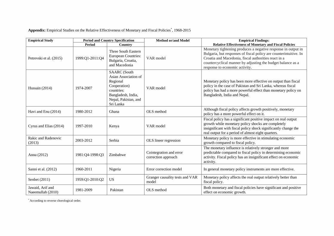
Appendix: Empirical Studies on the Relative Effectiveness of Monetary and Fiscal Policies*, 1968-2015

Empirical Study Period and Country Specification Method or/and Model

Empirical Findings:

Relative Effectiveness of Monetary and Fiscal Policies Period Country

Petrevski et al. (2015) 1999:Q1-2011:Q4

Three South Eastern

European Countries:

Bulgaria, Croatia,

and Macedonia

VAR model

Monetary tightening produces a negative response in output in

Bulgaria, but responses of fiscal policy are counterintuitive. In

Croatia and Macedonia, fiscal authorities react in a

countercyclical manner by adjusting the budget balance as a

response to economic activity.

Hussain (2014) 1974-2007

SAARC (South

Asian Association of

Regional

Cooperation)

countries:

Bangladesh, India,

Nepal, Pakistan, and

Sri Lanka

VAR model

Monetary policy has been more effective on output than fiscal

policy in the case of Pakistan and Sri Lanka, whereas fiscal

policy has had a more powerful effect than monetary policy on

Bangladesh, India and Nepal.

Havi and Enu (2014) 1980-2012 Ghana OLS method Although fiscal policy affects growth positively, monetary

policy has a more powerful effect on it.

Cyrus and Elias (2014) 1997-2010 Kenya VAR model

Fiscal policy has a significant positive impact on real output

growth while monetary policy shocks are completely

insignificant with fiscal policy shock significantly change the

real output for a period of almost eight quarters.

Rakic and Radenovic

(2013) 2003-2012 Serbia OLS lineer regression

Monetary policy is more effective in stimulating economic

growth compared to fiscal policy.

Anna (2012) 1981:Q4-1998:Q3 Zimbabwe Cointegration and error

correction approach

The monetary influence is relatively stronger and more

predictable compared to fiscal policy in determining economic

activity. Fiscal policy has an insignificant effect on economic

activity.

Sanni et al. (2012) 1960-2011 Nigeria Error correction model In general monetary policy instruments are more effective.

Senbet (2011) 1959:Q1-2010:Q2 US Granger causality tests and VAR

model

Monetary policy affects the real output relatively better than

fiscal policy.

Jawaid, Arif and

Naeemullah (2010) 1981-2009 Pakistan OLS method

Both monetary and fiscal policies have significant and positive

effect on economic growth.

* According to reverse chorological order.

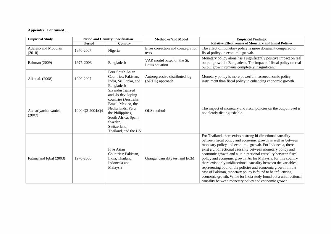
Appendix: Continued…

Empirical Study Period and Country Specification Method or/and Model

Empirical Findings:

Relative Effectiveness of Monetary and Fiscal Policies Period Country

Adefeso and Mobolaji

(2010) 1970-2007 Nigeria

Error correction and cointegration

tests

The effect of monetary policy is more dominant compared to

fiscal policy on economic growth.

Rahman (2009) 1975-2003 Bangladesh VAR model based on the St.

Louis equation

Monetary policy alone has a significantly positive impact on real

output growth in Bangladesh. The impact of fiscal policy on real

output growth remains completely insignificant.

Ali et al. (2008) 1990-2007

Four South Asian

Countries: Pakistan,

India, Sri Lanka, and

Bangladesh

Autoregressive distributed lag

(ARDL) approach

Monetary policy is more powerful macroeconomic policy

instrument than fiscal policy in enhancing economic growth.

Atchariyachanvanich

(2007)

1990:Q2-2004:Q4

Six industrialized

and six developing

countries (Australia,

Brazil, Mexico, the

Netherlands, Peru,

the Philippines,

South Africa, Spain

Sweden,

Switzerland,

Thailand, and the US

OLS method The impact of monetary and fiscal policies on the output level is

not clearly distinguishable.

Fatima and Iqbal (2003) 1970-2000

Five Asian

Countries: Pakistan,

India, Thailand,

Indonesia and

Malaysia

Granger causality test and ECM

For Thailand, there exists a strong bi-directional causality

between fiscal policy and economic growth as well as between

monetary policy and economic growth. For Indonesia, there

exist a unidirectional causality between monetary policy and

economic growth and a unidirectional causality between fiscal

policy and economic growth. As for Malaysia, for this country

there exist only unidirectional causality between the variables

representing both of the policies and economic growth. In the

case of Pakistan, monetary policy is found to be influencing

economic growth. While for India study found out a unidirectional

causality between monetary policy and economic growth.

Appendix: Continued…

Empirical Study Period and Country Specification Method or/and Model

Empirical Findings:

Relative Effectiveness of Monetary and Fiscal Policies Period Country

Ajisafe and Folorunso

(2002) 1970-1998 Nigeria

Cointegration and error

correction modelling techniques

Monetary policy rather than fiscal policy exerts a great impact

on economic activity.

Jayaraman (2002)

Fiji (1980-1995),

Samoa (1983-

1995),

Tonga (1983-

1995),

Vanuatu (1984-

1995)

Four South Pacific

Island Countries:

Fiji, Samoa, Tonga

and Vanuatu

OLS method

Fiscal policies are effective in any of the four countries for

promoting economic growth. In Samoa, in particular, both fiscal

and monetary policies have no influence on growth. In Fiji,

Tonga and Vanuatu, monetary policy has a positive impact on

growth. In short, fiscal policies are found to be less effective.

Olaloye and Ikhide (1995) 1986 -1991

Nigeria OLS method

Fiscal policy exerts more influence on the economy than

monetary policy.

Owoye and Olugbenga

(1994) 1960-1990

Ten African

countries: Burundi,

Ethiopia, Ghana,

Kenya, Morocco,

Nigeria, Sierra

Leone, South Africa,

Tanzania and

Zambia

VAR model

Monetary policy is more important than fiscal policy in the half

of countries. However, for the other half of countries fiscal

policy is more important than monetary policy.

Kretzmer (1992) 1950:Q2-1979:Q4

1962:Q2-1991:Q4 US VAR model

Monetary policy becomes less effective over time, but is still

more effective than fiscal policy.

Looney (1989) 1965-1985 Saudi Arabia Macroeconomic simulation

model

The relationship between money and economic activity is more

predictable than that stemming from changes in autonomous

expenditures.

Chowdhury (1988) 1966:Q1-1984:Q4

Six European

Countries: Austria,

Belgium, Denmark,

The Netherlands,

Norway, and

Sweden

OLS method

Monetary policy, rather than fiscal policy, appears to have a

stronger as well as more predictable effect on GNP in Denmark,

Norway, and Sweden. However, in the case of Belgium and the

Netherlands, fiscal policy appears to have a greater influence on

economic activity but the results are inconclusive for the case of

Austria.

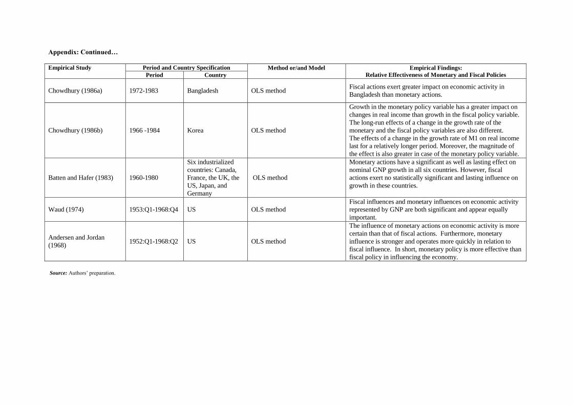
Appendix: Continued…

Empirical Study Period and Country Specification Method or/and Model

Empirical Findings:

Relative Effectiveness of Monetary and Fiscal Policies Period Country

Chowdhury (1986a) 1972-1983

Bangladesh

OLS method Fiscal actions exert greater impact on economic activity in

Bangladesh than monetary actions.

Chowdhury (1986b) 1966 -1984 Korea OLS method

Growth in the monetary policy variable has a greater impact on

changes in real income than growth in the fiscal policy variable.

The long-run effects of a change in the growth rate of the

monetary and the fiscal policy variables are also different.

The effects of a change in the growth rate of M1 on real income

last for a relatively longer period. Moreover, the magnitude of

the effect is also greater in case of the monetary policy variable.

Batten and Hafer (1983) 1960-1980

Six industrialized

countries: Canada,

France, the UK, the

US, Japan, and

Germany

OLS method

Monetary actions have a significant as well as lasting effect on

nominal GNP growth in all six countries. However, fiscal

actions exert no statistically significant and lasting influence on

growth in these countries.

Waud (1974) 1953:Q1-1968:Q4 US OLS method

Fiscal influences and monetary influences on economic activity

represented by GNP are both significant and appear equally

important.

Andersen and Jordan

(1968) 1952:Q1-1968:Q2 US OLS method

The influence of monetary actions on economic activity is more

certain than that of fiscal actions. Furthermore, monetary

influence is stronger and operates more quickly in relation to

fiscal influence. In short, monetary policy is more effective than

fiscal policy in influencing the economy.

Source: Authors’ preparation.