Transiting Planet Analysis Tutorial

In this tutorial, you will learn how astronomers find and measure the size of new planets using the transit technique. In order to do this, you will be introduced to two web archives that you will use to get the data you need, and we will reinforce some of the techniques you used previously to analyze data with Excel.

Section 1: Query the MAST K2 Archive for lightcurves

The most successful telescope for finding planet transits is the NASA Kepler telescope. Here, we’re going to go to the public source for the most current Kepler data and look for planet transits.

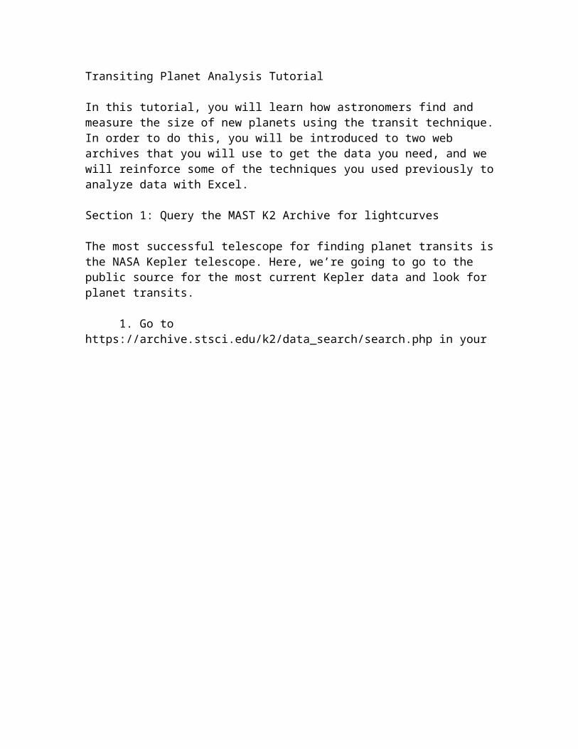
1. Go to https://archive.stsci.edu/k2/data_search/search.php in your web browser. The page should look like this:

2. Decide which star lightcurves you’d like to search for planets. To make things simple for now, we’re going to start with a star I already know well. This star’s K2 ID is 211351816. In the appropriate box, type this number. Then, hit the Search button at the bottom left of this page.

3. You should get a page titled “K2 Search Results.” 211351816 should be the only result in the table. Click on the link underneath “Dataset Name” in the table.

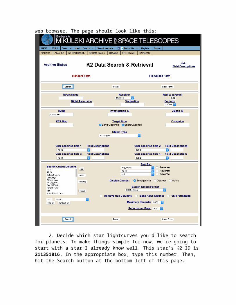
4. This should lead you to a page titled “K2 Preview for ….” There should also be a plot on this page with both a green and a pink curve.

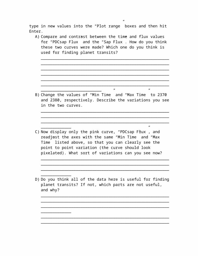
The red circles represent the changeable parameters in the plot. If you’d like to display one or both of the lightcurves, adjust these parameters, and then hit the “Start again” button and the plot will readjust its range (in the green circle). To

change the range of the plots, type in new values into the “Plot range” boxes and then hit Enter.

A) Compare and contrast between the time and flux values for “PDCsap Flux” and the “Sap Flux”. How do you think these two curves were made? Which one do you think is used for finding planet transits? ____________________________________________________________________________________________________________________________________________________________________________________________________________________________________________________________________________________________________________________________________________________________________

B) Change the values of “Min Time” and “Max Time” to 2370 and 2380, respectively. Describe the variations you see in the two curves.__________________________________________________________________________________________________________________________________________________________________________________

C) Now display only the pink curve, “PDCsap Flux”, and readjust the axes with the same “Min Time” and “Max Time” listed above, so that you can clearly see the point to point variation (the curve should look pixelated). What sort of variations can you see now?__________________________________________________________________________________________________________________________________________________________________________________

D) Do you think all of the data here is useful for finding planet transits? If not, which parts are not useful, and why?____________________________________________________________________________________________________________________________________________________________________________________________________________________________________________________________________________________________________________________________________________________________________

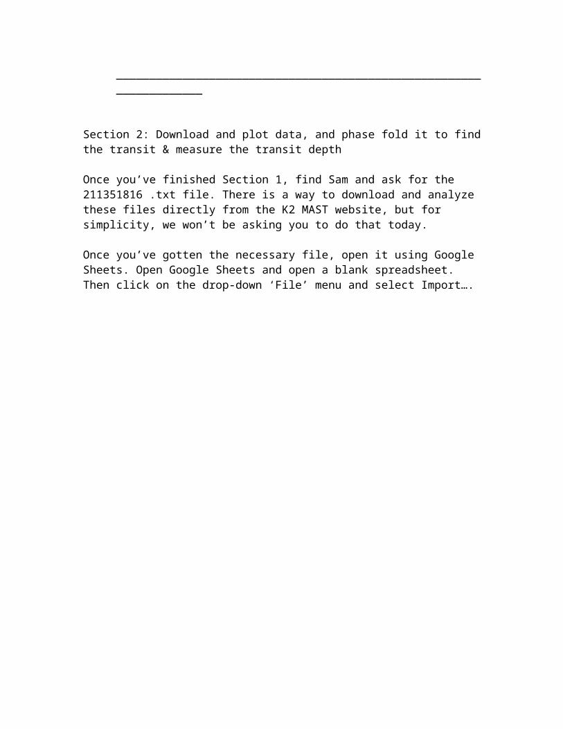
Section 2: Download and plot data, and phase fold it to find the transit & measure the transit depth

Once you’ve finished Section 1, find Sam and ask for the 211351816 .txt file. There is a way to download and analyze these files directly from the K2 MAST website, but for simplicity, we won’t be asking you to do that today.

Once you’ve gotten the necessary file, open it using Google Sheets. Open Google Sheets and open a blank spreadsheet. Then click on the drop-down ‘File’ menu and select Import….

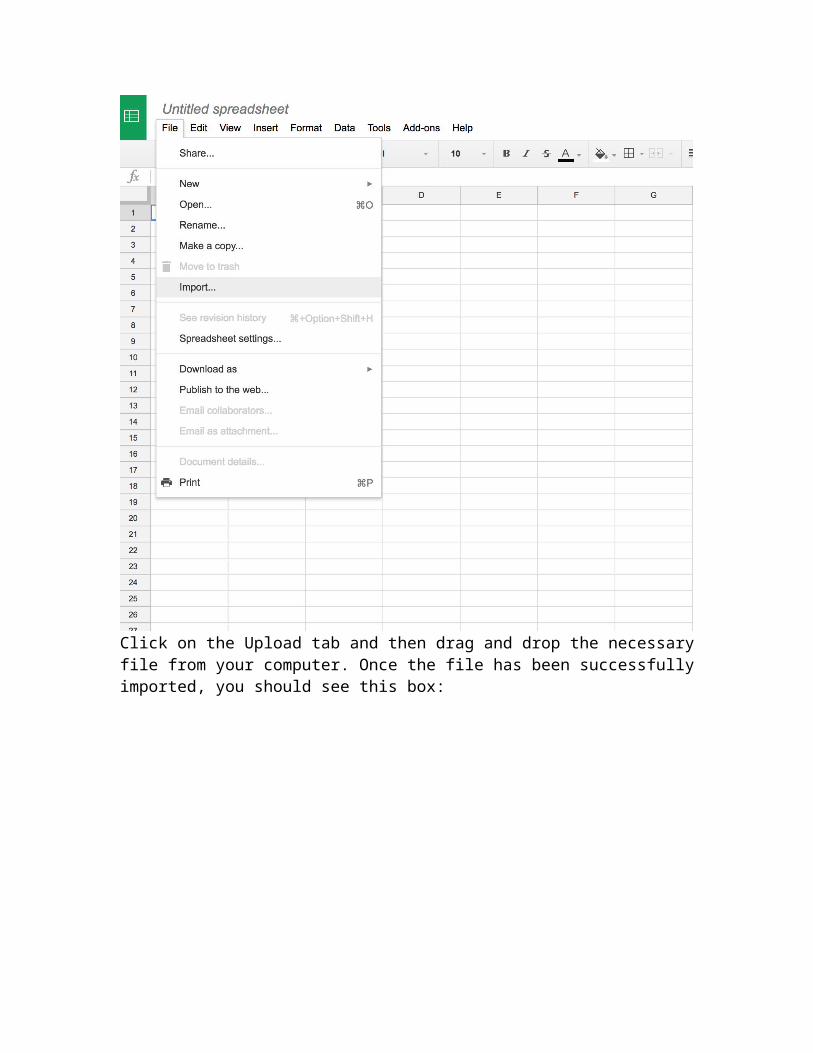
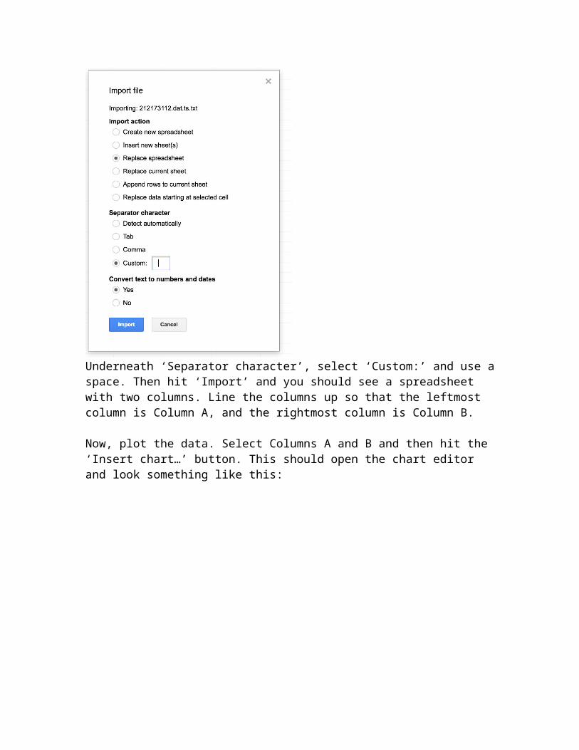
Click on the Upload tab and then drag and drop the necessary file from your computer. Once the file has been successfully imported, you should see this box:

Underneath ‘Separator character’, select ‘Custom:’ and use a space. Then hit ‘Import’ and you should see a spreadsheet with two columns. Line the columns up so that the leftmost column is Column A, and the rightmost column is Column B.

Now, plot the data. Select Columns A and B and then hit the ‘Insert chart…’ button. This should open the chart editor and look something like this:

Now go to chart types, and make sure the box that says ‘Use Column A as labels’ is

checked and that the plot is either a line or scatter plot. Then, hit ‘Insert’. You should now have made a plot of your lightcurve.

Notice that these lightcurves similarly has axes of Time and Flux, but here, flux is not measured in electrons per second (e-/sec). Instead, the flux values have been “normalized”. This means that the average flux value for this dataset is equal to 1, and all changes in flux are measured relative to the average.

A) How is this different from what we saw in the K2 MAST Archive (Section 1)? Will this make the transit depth easier to measure? Why or why not?________________________________________________________________________________________________________________________________________________________________________

The next step will be to phase fold your data and line up multiple transits. To do this, we’ll be using the Google Sheets MOD() function. Go to the C1 cell and type ‘=MOD(A1, period)’ where period is your guess for the period of the planet. Then, copy and paste until you’ve created another array of times that’s as long as Column A. Also, copy and paste Column B into Column D (without any changes). Then repeat what you had done earlier to create a plot of your (now phase-folded) lightcurve. Can you see the transit?

Once you’ve gotten all of your transits lined up, you can measure the transit depth of this planet. Estimate the normalized flux at the center of transit, and subtract it from 1 to find the planet transit depth: __________________________

A) Why couldn’t we only use one transit to measure the transit depth?_________________________________________________________________________________B) How is transit depth related to the planet to star radius ratio? Hint: Remember a star’s shape on the plane of the sky.__________________________________________________________________________________C) Can we use the transit depth alone to measure the planet radius? Why or why not?__________________________________________________________________________________D) What other features of the transit or lightcurve might tell us something about the planet or star?__________________________________________________________________________________

Section 3: Use the NASA Exoplanet Archive to find stellar parameters and calculate planet size.

1. Go to https://exoplanetarchive.ipac.caltech.edu/ in your web browser. There should be a box entitled “Explore the Archive” on the upper left hand side with a “Search” engine inside. Type “EPIC 211351816” into the appropriate space, and then hit “Search”. This should bring you to a page that looks like this:

The two red circles show the two table sections we’re going to be using.Scroll down to display everything in the “Summary of Stellar Information” table section.

A) What is the stellar radius? ____________________________Now turn to the “Planet Transit Properties” table section.

B) What is the Ratio of Planet to Stellar Radius?_________________________Does this match with what you calculated for the transit depth in the previous section? If not, why not?________________________________________________________________________________________________________________________________________________________________________Use this to calculate the planet radius in solar radii. _________________________Does this match with what is given in the “Planet Parameters” section?____

How will you use this knowledge in the next week? What other systems are you interested in investigating? ___________________________________________________________________________________________________________________________________________________________________________________________________________________________________________________________________________