Supporting Information forSingle Molecule Spectroscopy of Amino Acids and Peptides by

Recognition TunnelingYanan Zhao, Peiming Zhang, Brian Ashcroft, Hao Liu, Suman Sen, Weisi Song,

JongOne Im, Brett Gyarfas , Saikat Manna, Sovan Biswas, Chad Borges and Stuart Lindsay

Page2 1. Figure S1: Binding of D-ASN by ICA molecules3-5 2. Figure S2: RT current traces for 18 amino acids6 3. Figure S3: RT current traces for tyrosine and tryptophan 7 4. Table S1: Starting Features8 5. Figure S4: Heat map of correlation coefficients between starting features9 6. Table S2: Features that remain after replacing highly correlated groups10 7. Table S3: Features that remain after removing run-to-run sensitive and

analyte insensitive features.11 8. Figure S5: Accuracy as a function of the degree of broadening of the

common data filter.12 9. Table S4a: 52 features used to generate Table 112 Table S4b: Ranked significance of 10 most important signal features13 10. Figure S6: RT signals from peptides13 11. Table S5a: Distribution of calls among peptides and amino acids13 Table S5b: Separation of three peptides14 12. Figure S7: RT signals from sequential flow of analytes14 13. Figure S8: Example of correction for instrumental frequency response.15 14. Figure S9: STM image of Pd grains15 15. Figure S10a: Distribution of cluster lengths by spikes16 Figure S10b: Distribution of cluster lengths by times17 16. Electrospray MS of ICA-amino acid solutions19 Table S6: ESIMS data for individual amino acids and ICA20 Table S7: ESIMS data for 1:1 and 1:2 adducts and MS-MS data21 Figure S11: ESIMS spectra of pure compounds and complexes22 Figure S12: Examples of MS-MS spectra23 Figure S13: RT signals from asparagine in pure water23 17. Interactions of a dipeptide with ICA on a gold substrate25 Figure S14: Force spectra26 18. Analysis of correlations within signal clusters28 Figure S15: Correlation values within clusters for the top 24 parameters28 Table S8: Parameter values for Figure S1529 19. Clustering of data values and bonding29 Table S9: Number of data clusters in 24 parameter space30 Figure S16: 2D projections of data clustering

1

Figure S1: Binding of D-ASN in a RT junction. As in Figure 1a, the arrow shows the molecular dipole, tilted relative to that for L-ASN. The structures shown here and in Figure 1 were calculated using DFT (B3LTY/6-311++G (2df,2p), Spartan ’10 Software) with the distance between the two sulfur atoms constrained to be 2 nm.

2

Figure S2a: RT current traces for the charged amino acids, tunnel gap set to 4 pA at 0.5V bias with 100μM solutions in 1 mM phosphate buffer, pH 7.4. A trace for buffer alone is shown as the control in the upper left.

3

Figure S2b: RT current traces for the hydrophobic amino acids (excluding tyrosine and tryptophan). Tunnel gap set to 4 pA at 0.5V bias with 100μM solutions in 1 mM phosphate buffer.

4

Figure S2c: RT current traces for the remaining amino acids (excluding tyrosine and tryptophan). Tunnel gap set to 4 pA at 0.5V bias with 100μM solutions in 1 mM phosphate buffer. A trace for buffer alone is shown as the control in the upper left. The arrow points to a “water” spike.

5

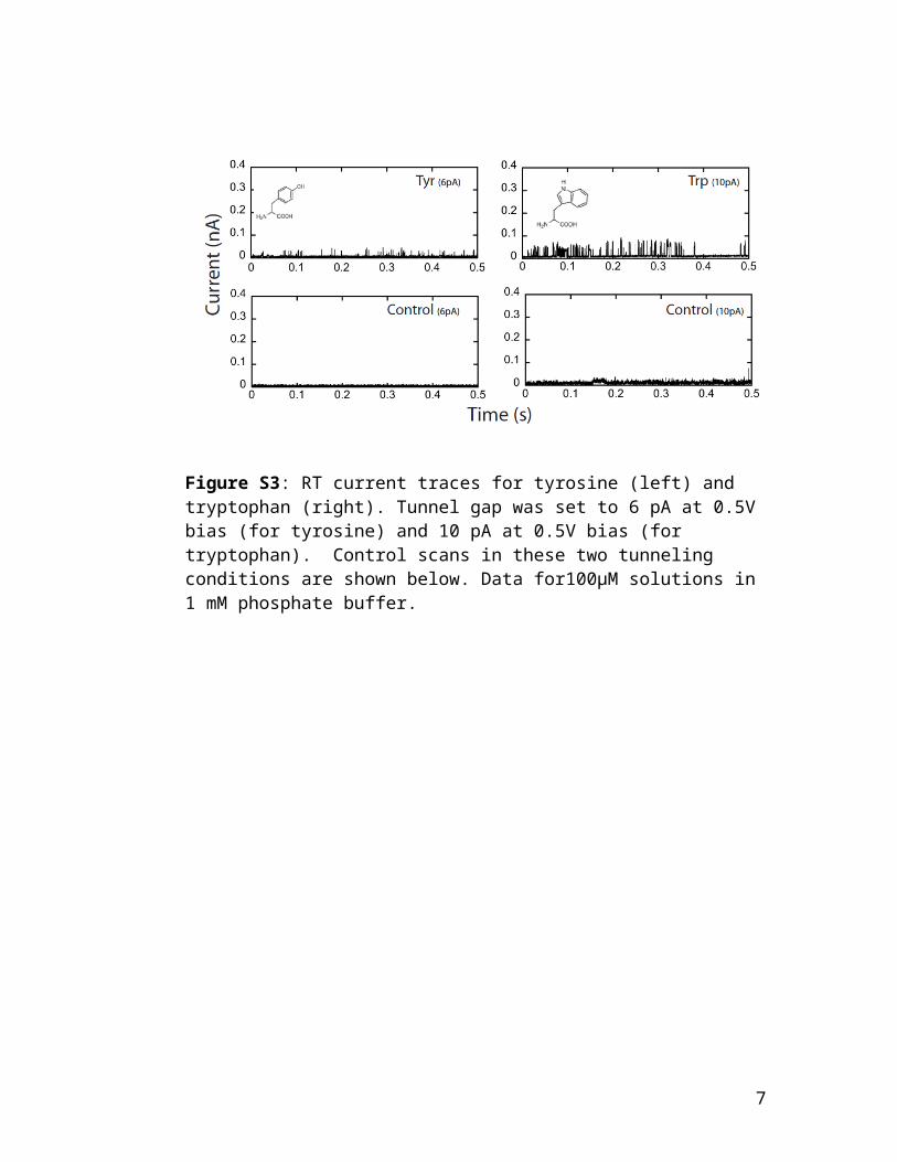
Figure S3: RT current traces for tyrosine (left) and tryptophan (right). Tunnel gap was set to 6 pA at 0.5V bias (for tyrosine) and 10 pA at 0.5V bias (for tryptophan). Control scans in these two tunneling conditions are shown below. Data for100μM solutions in 1 mM phosphate buffer.

6

Feature Number

Feature Name Feature Description

1 Max Amplitude Maximum current at the peak2 Average Amplitude Average of all the spike3 Top Average Fig. 4d average of peak above half maximum4 Spike Width full width at half maximum5

Roughness standard deviation of the spike above half maximum height

6 Total FFT Power Square root of the sum of power spectrum7

FFT L Average of three points within the first frequency band (0.9, 1.8, 2.7 kHz)

8FFT M Average of three points within the middle frequency

band (9.3, 10.2, 11.1 kHz)9

FFT H Average of three points within the highest frequency band (23.2, 24.1, 25 kHz)

10High Low Ratio Fig. 4g Ratio of FFT amplitude in the 22.3-25 kHz band to that

in the 0- 2.7 kHz band11

Spike Frequency Number of peaks per milisecond over a window of 4096 samples

12Odd FFT Components Summ of all odd frequencies from the non

downsampled FFT13

Even FFT Components Sum of all even frequencies from the non downsampled FFT

14 Odd Even Ratio Ratio of the odd to the even FFT sums15-23 Spike FFT Components (1-9)

#15 – Figs. 4a and h,#21 Fig. 4b, #20 – Fig. 4e Downsampled FFT spectrum

24 Spikes In Cluster Number of peaks in the cluster25

Cluster Peak Frequency Number of peaks in cluster divided by ms length of cluster

26 Cluster Average Amplitude Fig. 3a Average amplitude of all cluster peaks

27 Cluster Top Amplitude Average amplitude of all peaks above half maximum28 Cluster Width Cluster time in ms29 Cluster Roughness std deviation of whole cluster signal30 Cluster Max Amplitude average of the max of all the spikes in cluster31 Cluster Total FFT Power square root of the sum of the power spectrum32

Cluster FFT Low Average of three points within the first frequency band (0.136, 0.273, 0.410 kHz)

33Cluster FFT Medium Average of three points within the middle frequency

band (12.710, 12.847, 12.983 kHz)34

Cluster FFT High Average of three points within the highest frequency band (24.726, 24.863, 25 kHz)

35-95 Cluster FFT Components (1-61)#55 – Fig. 3b, #89 – Fig. 3c Downsampled FFT spectrum of cluster

96-99 Cluster Frequency Location of Maximum Peaks (1-4)

Frequency of the 4 dominant peaks in the spectrum, ordered by the height of the peaks

100-161Cluster Cepstrum (1-61) Spectrum of the power spectrum of the cluster,

downsampled to 61 points

Table S1: 161 starting features used in the signal analysis. Details of their calculation are given in Chang et al.1 Bold entries mark features used in the figures.

7

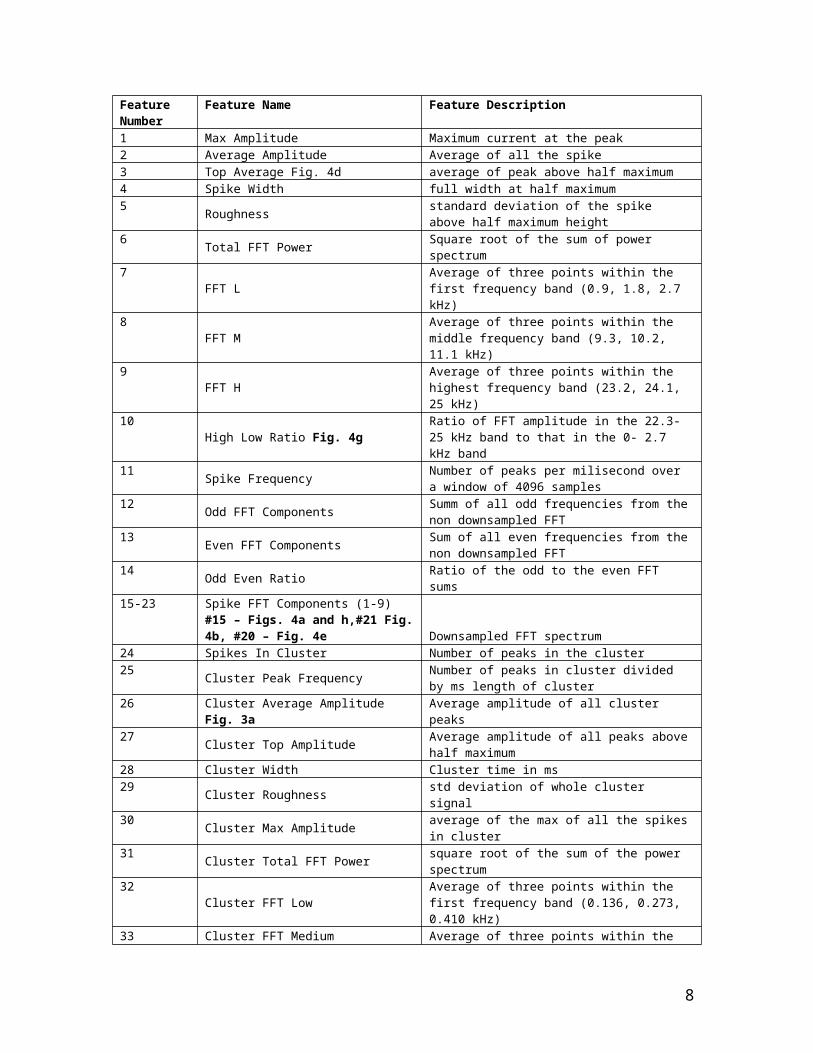
Figure S4: Correlation map for all 161 features. Each axis lists the feature number as labeled in Table 1. Blue = -1, red = +1. The large red region in the middle reflects a high degree of correlation among the higher frequency cluster FFT components. The cluster FFT amplitude for 22.6 to 23 kHz was used in the analysis shown in Fig. as representative of the group.

8

Table S2: Features with ≥ removed by the correlation test. Here, the group of cluster FFTs was replaced with FFT60. In Fig. 3, FFT 57 was used. For FFT amplitude calculations, a minimum data size of 512 points was used. Peaks that were less than 512 data points in extent were padded with zeroes on each side to bring the input data to 512 points. In the case of cluster FFTs, zero padding was again employed to ensure that the shorter traces were at least 4096 samples.

9

FeatureMax AmplitudeAverage AmplitudeHighLowRatioOdd-FFTEven-FFTClusterInfo.Top AmplitudeClusterInfo.Peaks In ClusterClusterInfo.Cluster FFT24ClusterInfo.Cluster FFT25ClusterInfo.Cluster FFT26ClusterInfo.Cluster FFT27ClusterInfo.Cluster FFT28ClusterInfo.Cluster FFT29ClusterInfo.Cluster FFT30ClusterInfo.Cluster FFT31ClusterInfo.Cluster FFT34ClusterInfo.Cluster FFT35ClusterInfo.Cluster FFT36ClusterInfo.Cluster FFT37ClusterInfo.Cluster FFT38ClusterInfo.Cluster FFT39ClusterInfo.Cluster FFT40ClusterInfo.Cluster FFT41ClusterInfo.Cluster FFT42ClusterInfo.Cluster FFT43ClusterInfo.Cluster FFT44ClusterInfo.Cluster FFT45ClusterInfo.Cluster FFT46ClusterInfo.Cluster FFT47ClusterInfo.Cluster FFT48ClusterInfo.Cluster FFT49ClusterInfo.Cluster FFT50ClusterInfo.Cluster FFT54ClusterInfo.Cluster FFT55ClusterInfo.Cluster FFT56ClusterInfo.Cluster FFT57ClusterInfo.Cluster FFT58ClusterInfo.Cluster FFT59ClusterInfo.Cluster FFT61ClusterInfo.Cluster Cepstrum61

FeatureFrequencyPeak FreqPeak-FFT-4Peak-FFT-5ClusterInfo.RoughnessClusterInfo.iFFT LowClusterInfo.Freq Maximum Peaks2ClusterInfo.Freq Maximum Peaks3ClusterInfo.Cluster Cepstrum35ClusterInfo.Cluster Cepstrum3ClusterInfo.Cluster Cepstrum43ClusterInfo.Cluster Cepstrum49ClusterInfo.Cluster Cepstrum54ClusterInfo.Cluster FFT14ClusterInfo.Cluster FFT17

Table S3: Features removed as the bottom 15 in the ranking of out of-group fluctuations to in group fluctuations.

10

Figure S5: Scatter plot of the average accuracy for calling all seven analytes from a single spike as a function of the percent of data rejected as common by broadening the soft margins of the SVM rejection filter. Repeated points are for different feature combinations. There is a “sweet point” at about 30% data retention. Further filtering of common signals does little to improve accuracy beyond this point.

11

ClusterInfo.Average Amplitude| ClusterInfo.Cluster Width| ClusterInfo.Roughness| ClusterInfo.Amplitude| ClusterInfo.Total Power| ClusterInfo.iFFT Low| ClusterInfo.iFFT Medium| ClusterInfo.iFFT High| ClusterInfo.Cluster FFT6| ClusterInfo.Cluster FFT7| ClusterInfo.Cluster FFT8| ClusterInfo.Cluster FFT9| ClusterInfo.Cluster FFT10| ClusterInfo.Cluster FFT11| ClusterInfo.Cluster FFT15| ClusterInfo.Cluster FFT16| ClusterInfo.Cluster FFT18| ClusterInfo.Cluster FFT19| ClusterInfo.Cluster FFT20| ClusterInfo.Cluster FFT22| ClusterInfo.Cluster FFT60| ClusterInfo.Freq Maximum Peaks3| ClusterInfo.Freq Maximum Peaks4| ClusterInfo.Cluster Cepstrum1| ClusterInfo.Cluster Cepstrum8| ClusterInfo.Cluster Cepstrum10| ClusterInfo.Cluster Cepstrum15| ClusterInfo.Cluster Cepstrum16| ClusterInfo.Cluster Cepstrum17| ClusterInfo.Cluster Cepstrum22| ClusterInfo.Cluster Cepstrum25| ClusterInfo.Cluster Cepstrum28| ClusterInfo.Cluster Cepstrum30| ClusterInfo.Cluster Cepstrum31| ClusterInfo.Cluster Cepstrum33| ClusterInfo.Cluster Cepstrum34| ClusterInfo.Cluster Cepstrum35| ClusterInfo.Cluster Cepstrum36| ClusterInfo.Cluster Cepstrum37| ClusterInfo.Cluster Cepstrum40| ClusterInfo.Cluster Cepstrum41| ClusterInfo.Cluster Cepstrum42| ClusterInfo.Cluster Cepstrum44| ClusterInfo.Cluster Cepstrum47| ClusterInfo.Cluster Cepstrum48| ClusterInfo.Cluster Cepstrum50| ClusterInfo.Cluster Cepstrum52| ClusterInfo.Cluster Cepstrum56| ClusterInfo.Cluster Cepstrum57| ClusterInfo.Cluster Cepstrum58| ClusterInfo.Cluster Cepstrum60

Table S4a: 52 features used to generate the data shown in Table 1.

Signal Feature Relative SignificanceClusterInfo.Cluster Cepstrum6 0.990677933 ClusterInfo.Cluster Cepstrum7 0.969959584 ClusterInfo.Freq Maximum Peaks2 0.839620008ClusterInfo.Cluster FFT10 0.772294783ClusterInfo.Cluster Cepstrum7 0.666798047 ClusterInfo.Cluster Cepstrum19 0.659547261 ClusterInfo.Cluster Cepstrum48 0.652476787 ClusterInfo.Average Amplitude 0.504609478 ClusterInfo.Cluster Cepstrum53 0.402374029 ClusterInfo.Cluster Cepstrum21 0.387171343

Table S4b: Relative significance of the top ten signal features in assigning a;l seven amino acids.

12

Figure S6: Representative RT signals for (a) GGGG and (b) GGLL.

GLY_GLY_GLY_GLY GLY_GLY_LEU_LEU5 6

ARG_L 4.4 1.9ASN_D 3.8 1.4ASN_L 3.1 2.3GLY 0.1 1.5GLY_GLY_GLY_GLY 73.2 0.2GLY_GLY_LEU_LEU 5.3 87.5ILE 4.3 0.9LEU 0 0.2mGLY 5.9 4.0

Table S5a: Distribution of calls among the peptides and amino acids, showing percentages of the signal spikes from each peptide called as one of the seven amino acids, the correct peptide, or the wrong peptide. The vast majority of calls are correct (73 and 87%) showing how each peptide it distinct form the other and distinct from the amino acids.

CallsAnalyte GLY_GLY_GLY GLY_GLY_GLY_GLY GLY_GLY_LEU_LEUGLY_GLY_GLY 96.4497 1.7751 1.7751GLY_GLY_GLY_GLY 2.7027 97.2973 0GLY_GLY_LEU_LEU 9.9291 0 90.0709Table S5b: Separation of signals from three peptides. Samples are listed in the left hand column with the distribution of calls among the three possible calls listed in the three right columns. This accuracy was achieved with 65% of the signal spikes rejected as “common”.

13

Figure S7: Reading analytes sequentially, a possible basis for peptidase sequencing: 100μM glycine was first flushed into the gap and read for 2s. The gap was the flushed for ~ 1 minute (hash marks on time axis) and 100μM phenylalanine inserted at 6 s on this axis (but note time break). An SVM trained on this data run separated the two analytes correctly at a 96% true positive rate.

Figure S8: Correction for instrumental frequency response. Showing the amplitude distribution for FFT3 (5.6 – 8.3 kHz) for L- and D-ASN before (a) and after (b) correction of the Fourier amplitudes by division of the signals by the Fourier amplitudes of the background signal. Large differences between the analytes at low amplitudes were masked by the instrumental response in (a).

14

Figure S9: Grain structure of the Pd substrate as imaged with an insulated, functionalized Pd probe. Set point is 4 pA at 0.5V bias. Image size is 200 nm x 200 nm and height scale is 0-2 nm. Images like this were obtained before each run of RT data was collected.

Figure S10a: Cluster length distributions for (a) seven amino acids. The distribution is exponential with a characteristic length of 20 spikes. (b) For peptides and glycine (as marked). There is less data, but the peptides GGG and GGLL appear to have some longer runs in the tail of the distribution.

15

1 31 61 91121

151181

211241

271301

331361

391421

451481

1

10

100

1000

10000

'ARG_L''ASN_D''ASN_L''GLY''GLY_GLY_GLY''GLY_GLY_GLY_GLY''GLY_GLY_GLY_T''GLY_GLY_LEU_LEU''ILE''LEU''mGLY'

Duration(ms)

Figure S10b: Distribution of cluster durations in ms for all 7 amino acids and four peptides. The 1/e time for the distributions is about 200 ms. The spike near 80 mS is an artifact of the data analysis which placed all short clusters into this first bin.

16

16.1 Electrospray MS of ICA-amino acid solutions

We have studied the interactions of ICA with amino acids by means of electrospray

ionization (ESI) mass spectrometry. ESI is able to transfer weakly bound complexes to

the gas phase for mass analysis. It has been used to study noncovalent interactions, for

example inclusion compounds of cyclodextrins, 2,3 serine clusters,4,5 hydrogen bonding

complexes,6 and π stacking complexes.7 Many studies have demonstrated that the results

of ESI-MS analysis reflect the equilibria in solution.8-10 ESI should give us a snapshot of

the chemical species in the solution.11 Our focus in the present study was to determining

if the ICA molecule interacts with amino acids to form stoichiometric complexes. We

began with recording ESI mass spectra of individual amino acid and ICA aqueous

solutions and assigned their observed characteristic m/z peaks (Table S6). The ESI mass

data show that both ICA and amino acids can exist in both monomer and self-associated

adduct forms including dimers and trimers. Based on the measured pH of each solution,

we have deduced the major form of the analyte occurring in the solution according to its

reported pKa (see table S6). Under our experimental conditions, the ICA molecule stayed

neutral.12 Sequentially we mixed ICA with seven amino acids respectively in 1:1 and 2:1

ratios, and measured their ESI mass spectra. Examples of spectra from an ICA-Leu

mixture and the corresponding ICA and Leu solutions are given in Figure S11. By

comparing these spectra, we can clearly see two new m/z peaks appearing in the spectra

of the ICA-Leu mixture, which correspond to their 1:1 and 2:1 adducts. We confirm the

complexes by tandem mass spectrometry (ESIMS/MS, examples are given in Figure

S12). It should be noted that an ICA disulfide species (ICA’) existed in all of the

measured solutions due to oxidation of the thiol during the sample handling process

although we tried to avoid the oxidation using the argon sparging. ICA’ also formed the

1:1 adducts with amino acids. However, the ICA’ adducts can readily be distinguished

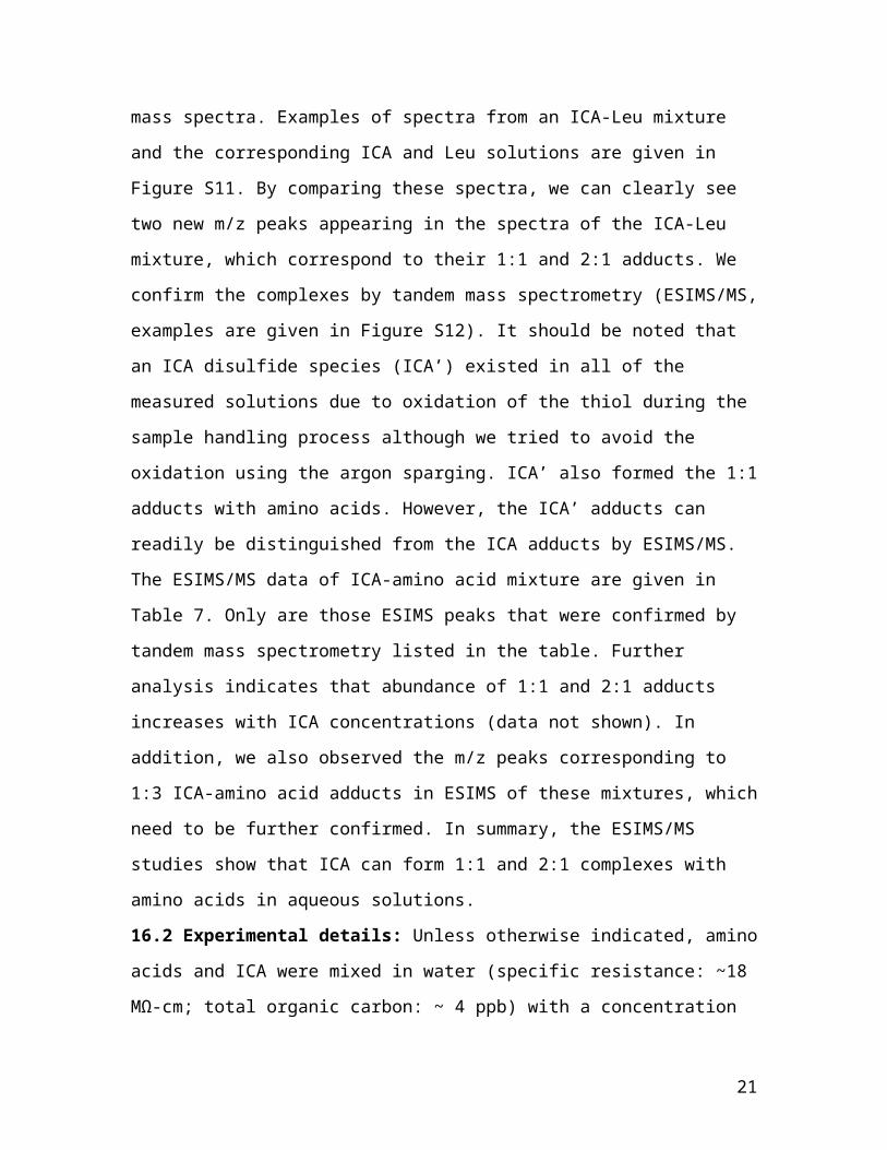
from the ICA adducts by ESIMS/MS. The ESIMS/MS data of ICA-amino acid mixture

are given in Table 7. Only are those ESIMS peaks that were confirmed by tandem mass

spectrometry listed in the table. Further analysis indicates that abundance of 1:1 and 2:1

adducts increases with ICA concentrations (data not shown). In addition, we also

17

observed the m/z peaks corresponding to 1:3 ICA-amino acid adducts in ESIMS of these

mixtures, which need to be further confirmed. In summary, the ESIMS/MS studies show

that ICA can form 1:1 and 2:1 complexes with amino acids in aqueous solutions.

16.2 Experimental details: Unless otherwise indicated, amino acids and ICA were

mixed in water (specific resistance: ~18 MΩ-cm; total organic carbon: ~ 4 ppb) with a

concentration of 100 µM each, sparged with argon. Buffers were not used and solution

pH’s are listed in the Tables. We checked that the omission of buffer slats does not affect

the acquisition of RT signals, by obtaining RT signals from asparagine in pure water

(Figure S13).

Each mixture was infused at 1 µL/min via syringe pump into a Bruker MicrOTOF-Q

electrospray ionization quadrupole time-of-flight (ESI-Q-TOF) mass spectrometer. The

ESI source was equipped with a microflow nebulizer needle operated in positive ion

mode. The spray needle was held at ground and the inlet capillary set to -4100 V. The

end plate offset was set to -500 V. The nebulizer gas and dry gas (N2) were set to 0.4 Bar

and 1.2 L/min, respectively, and the dry gas was heated to 180 °C. In TOF-only mode the

quadrupole ion energy was set to 8 eV and the collision energy was set to 10 eV.

Collision gas (Ar) was set to a flow rate of 15%. In most cases MS/MS experiments were

conducted with a precursor ion isolation width of 3 m/z units. However, if other ions

were present in this range precursor ion isolation width was set to 1 m/z unit. Collision

energy was set to 10 eV. Notably, this energy was sufficient to fragment non-covalent

complexes, but insufficient to break apart the disulfide-bonded dimer form of the ICA

reader. Due to the lack of an acid modifier in the infused solutions, most amino acids and

molecular complexes were observed as single or multiply sodium ions [M + nNa – (n-

1)H]+ rather than as protonated molecules [M + H]+. Average mass accuracy was within

0.025 Da.

18

Table S6. Structure information and MS data of Individual Amino Acids and ICA

AnalyteCalculated

Monoisotopic Mass

Solution pH Molecular form 1 Observed m/z

L-Leu 131.0946 8.1154.04, [M+Na]+, (82)176.03, [M+2Na-H] +, (85)285.16, [2M+Na] +, (100)

L-Ile 131.0946 8.0154.04, [M+Na]+, (65)176.03, [M+2Na-H] +, (100)285.16, [2M+Na] +, (50)

L-Asn 132.0535 8.1

155.00, [M+Na]+, (100)176.99, [M+2Na-H] +, (98)287.09, [2M+Na] +, (23)485.10, [3M+4Na-3H] +, (81)

D-Asn 132.0535 8.1

155.00, [M+Na]+, (34)176.99, [M+2Na-H] +, (66)287.07, [2M+Na] +, (11)485.09, [3M+4Na-3H] +, (100)

L-Gly 75.0320 7.8

97.96, [M+Na]+, (39)119.95, [M+2Na-H] +, (100)173.02, [2M+Na] +, (70)314.02, [3M+4Na-3H] +, (53)

N-MeGly 89.0477 7.9

111.98, [M+Na]+, (100)133.97, [M+2Na-H] +, (66)201.06, [2M+Na] +, (45)356.07, [3M+4Na-3H] +, (16)

L-Arg 174.1117 8.1

175.08, [M+H]+, (100)197.07, [M+Na]+, (37)219.05, [M+2Na-H] +, (23)371.20, [2M+Na] +, (57)

ICA 171.0466 8.3

172.02, [M+H]+, (8)194.01, [M+Na]+, (76)365.07, [2M+Na] +, (25)363.06, [ICA'+Na]+

1. The relative Intensity (%) value of observed ions are given in parentheses next to each complex ion. The most intense peaks in single stage MS spectra are defined as 100.

O

O

NH3

O

O

NH3

O

O

NH3

O

NH2

O

O

NH3

O

NH2

NH3

O

O

O

O

NH2

O

O

NH3

NH

H2N

NH2

N

NHHS

NH2

O

19

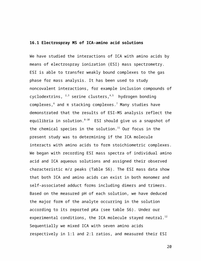
Table S7. Characteristic ESIMS of ICA-amino acids1:1 & 2:1 mixtures and their MS/MS products*

Analyte Observed m/z MS/MS Product Ion

Ratio pH Mass, adduct ion, (Intensity, S/N) Mass, molecular ion, (Intensity)

ICA+L-Leu1:1 7.8 325.12, [ICA+Leu+Na]+, (15.3, 1703) 194.00, [ICA+Na]+, (100)

2:1 7.9 518.16, [2ICA+Leu+2Na-H]+, (0.2, 80) 176.03, [Leu+2Na-H]+, (100)

ICA+L-Ile

1:1 7.8 325.12, [ICA+Ile+Na]+, (13.5, 1494) 194.00, [ICA+Na]+, (100)

2:1 7.9496.18, [2ICA+Ile+Na]+, (0.1, 42) 194.01, [ICA+Na]+, (100)

518.16, [2ICA+Ile+2Na-H]+, (0.2, 60) 176.03, [Ile+2Na-H]+, (100)

ICA+L-Asn

1:1 7.9 326.08, [ICA+L-Asn+Na]+, (6.1, 800) 155.00, [L-Asn+Na]+, (100)194.00, [ICA+Na]+, (5)

2:1 8.0497.13, [2ICA+L-Asn+Na]+, (0.5, 60) 365.06, [2ICA+Na]+, (100)

155.00, [L-Asn+Na]+, (48)

519.12, [2ICA+L-Asn+2Na-H]+, (0.4, 42) 176.99, [L-Asn+2Na-H]+, (100)

ICA+D-Asn1:1 7.9 326.08, [ICA+D-Asn+Na]+, (3.9, 691) 155.00, [D-Asn+Na]+, (100)

194.01, [ICA+Na]+, (5)

2:1 8.0 497.13, [2ICA+D-Asn+Na]+, (0.4, 67) 365.06, [2ICA+Na]+, (100)155.00, [D-Asn+Na]+, (74)

ICA+L-Gly1:1 8.0

269.05, [ICA+Gly+Na]+, (0.2, 53) 194.01, [ICA+Na]+, (100)172.02, [ICA+H]+, (24)

291.03, [ICA+Gly+2Na-H]+, (0.1, 30) 119.95, [Gly+2Na-H]+, (100)

2:1 8.1 462.10, [2ICA+Gly+2Na-H]+, (0.1, 24) 119.95, [Gly+2Na-H]+, (100)

ICA+N-MeGly1:1 8.0

261.09, [ICA+N-MeGly+H]+, (0.2, 23) 172.02, [ICA+H]+, (100)

283.07, [ICA+N-MeGly+Na]+, (0.4, 35) 194.00, [ICA+Na]+, (100)

2:1 8.1 476.11, [2ICA+N-MeGly+2Na-H]+, (0.1, 11) 133.97, [N-MeGly+2Na-H]+, (100)

ICA+L-Arg

1:1 7.8 346.16, [ICA+Arg+H]+, (0.2, 81) 175.09, [Arg+H]+, (100)

2:1 7.9517.21, [2ICA+Arg+H]+, (0.2, 59) 175.09, [Arg+H]+, (100)

539.19, [2ICA+Arg+Na]+, (0.3, 92) 197.07, [Arg+Na]+, (100)

20

21

Figure S12: Examples of MS-MS spectra. Two peaks are found in 2:1 mixtures of ICA with Leucine, circled in (a). MS-MS shows that the peak at 516 Daltons is a complex of an oxidized ICA (labeled ICA’) in which two ICA molecules are joined by a disulfide linkage (b). The peak at 518 Daltons is shown (c) to consist of two non-oxidized ICA molecules with one Leucine.

22

17.1 Interactions of a dipeptide with ICA on a gold substrate

We have studied the interactions of a dipeptide Cys-Gly with ICA on a single

molecule level by means of Force Spectroscopy. The ICA was bound to a gold-coated

mica surface through its thiolated linker. The dipeptide was attached to AFM tips through

an azido-(CH2CH2O)36-vinyl sulfone linker using a method developed in our laboratory.13

As shown in Scheme 1, the peptide was first reacted with the linker, yielding a

conjugate (1) containing an azide at its end, a functional group that was used for attaching

the dipeptide to AFM tips through a alkyne-azide click reaction13. Inspection of the

structure in scheme 1 suggests that the dipeptide could be capable of forming 3 or more

hydrogen bonds (the primary amine will be protonated and the carboxylate deprotonated

Figure S13: RT signals from asparagine in pure water.

Scheme 1

23

at neutral pH).

Meanwhile, a control molecule (2) containing an alkane chain at its end was

synthesized by reacting the same linker with hexanethiol, which should have no the

hydrogen bonding interactions with ICA.

An AFM tip functionalized with the dipeptide 1 was brought down to contact a

surface coated with ICA and then retracted back, and force-distance curves were

recorded. In each experiment, we collected one thousand five hundred curves. About

10% of these showed evidence of an event involving stretching of the PEG linker. Of

this subset, we retained only those curves that fitted a WLC extension curve14 with a

contour length of 15±3 nm and for which the baseline force had returned close to 0pN

after the peak owing to non-specific interactions. An example of a force curve satisfying

these criteria is shown in Figure S14a. We took over 500 force curves with the control

molecule (2 is scheme 1) and none shown of these controls evidence of specific binding

with all adhesion gone by 10 nm extension. We also measured the interactions of the

dipeptide (1) with a bare gold surface finding no force curves in which the PEG tether

was fully stretched.

Figure S14b shows a histogram of bond-breaking forces obtained from curves like

those in Figure S14a using a probe of force constant 0.05 N/m (SiN probes from Veeco

Probes) and a retraction speed of 700 nm/s. Using the data presented in Fuhrmann et

al.15, the modal breaking force for a complex involving 2 hydrogen bonds is about 22 pN,

and this is consistent with the data shown in this histogram. More specifically, taking the

force barrier, fB = 1/α, to be 5.8 pN (using the value for γ=1 from Fuhrmann et al.15), the

calculated distribution16 is shown by the solid line. Clearly many of the events are

consistent with two hydrogen bonds between the glycine and the ICA monolayer, though

events at both lower and higher forces indicate that other bonding motifs are possible

(and expected, given the structure of the peptide as discussed above).

24

17.2 Experimental details:

Synthesis of the dipeptide conjugate (1). To a solution of azido-(CH2CH2O)36-vinyl

sulfone (50 µL, 1.0 mM) in pH 8 phosphate buffer was added a solution of the dipeptide

(50 µL, 20 mM) in pH 8 phosphate buffer. The reaction was stirred for 3hrs at room

temperature, followed by RP-HPLC purification using a Zorbax C18 column on an

Agilent 1100 HPLC equipped with an ELSD detector under a gradient of 10 to 80%

Methanol in a 10 mM TEAA buffer (pH 7.0) over a period of 25 mins. The retention time

of the desired product was 12.6mins. The collected solution was lyophilized and

characterized by MALDI-MS on a Voyager MALDI-TOF instrument. MS: m/z (M+H)

calculated for C29H59+1N5O15S: 1948.28; found: 1948.01.

Synthesis of the control molecule (2). To a solution of azido-(CH2CH2O)36-vinyl

sulfone (50 µL, 1.0 mM) in DMSO was added a solution of hexanethiol (50 µL, 20 mM)

in DMSO and triethylamine (1 µL). The reaction was stirred for 3 hrs at room

temperature, followed by RP-HPLC purification using a Zorbax C18 column on an

Agilent 1100 HPLC equipped with an ELSD detector under of gradient of 10 to 80%

Methanol in a 10 mM TEAA buffer (pH7.0) over a period of 25 mins. The retention time

of the desired product was 19.8mins. The collected solution was lyophilized and

characterized by MALDI-MS on a Voyager MALDI-TOF instrument. MS: m/z (M+H)

calculated for C30H63+1N3O12S: 1888.31; found: 1888.03

Attachment. Both dipeptide conjugate 1 and control 2 were attached to AFM tips

(Veeco probes, Bruker, SiN tips, force constant 0.05 N/m) by an azide-alkyne click

reaction using N-(3-(silatranyl)propyl)-2-(cyclooct-2-yn-1-yloxy)acetamide as an

anchoring molecule in a two step protocol developed in our lab.1

Functionalization of Gold substrates. Gold-coated mica substrates (Au(111), 2.4 x

1.6 cm2, Agilent Technologies) were immersed in a solution of ICA (0.1 mM) in absolute

ethanol for 1day, followed by rinsing with ethanol and water, and used immediately for

AFM measurements.

AFM force measurement and data analysis. The force measurements were carried

out at a loading rate of 35 nN/s on an Agilent 5500 AFM using functionalized tips against

25

the ICA functionalized Gold substrates. Control experiments were performed using tips

functionalized with the dipeptide conjugate 1 against the bare Gold substrate and tips

functionalized with the control molecule 2 against the ICA coated Gold substrate. All the

experiments were carried out in 1X PBS buffer, pH 7.4. The force spectra were recorded

using Agilent Picoview software. Mathworks-MATLAB was used for data analysis,

plotting, and curve fitting.

18. Analysis of correlations within signal clusters

We define an index of correlation, S, as follows:

Sn=σ n

cluster

σ nall

where σ ncluster is the standard deviation of the values of the nth signal feature within

clusters and σ nall is the standard deviation of the values of the nth signal feature for

the entire data set, both normalized to the number of data points. For signal

features that are highly correlated within a cluster, σ ncluster → 0, so S→0. For feature

values distributed randomly, σ ncluster=σn

all, so S →1.

The calculated values of S for all seven amino acids are shown as a function of

feature number in Figure S15, for all 24 features used to describe single peaks. The

features corresponding to these numbers are listed in Table S8 below. Those

features that are strongly correlated within clusters (S→0) correspond to the

features most sensitive to bonding.

26

Table S8: Features in Figure S15# Feature 1 'maxAmplitude'2 'averageAmplitude'3 'topAverage'4 'peakWidth'5 'roughness'6 'totalPower'7 'iFFTLow'8 'iFFTMedium'9 'iFFTHigh'10 'frequency'11 'peakFFT1'12 'peakFFT2'13 'peakFFT3'14 'peakFFT4'

Figure S15: Features with low S values are highly correlated within clusters. Features numbers are listed with the associated signal features in the table below. Different colored lines are for different amino acids.

27

15 'peakFFT5'16 'peakFFT6'17 'peakFFT7'18 'peakFFT8'19 'peakFFT9'20 'peakFFT10'21 'highLow_Ratio'22 'Odd_FFT'23 'Even_FFT'24 'OddEvenRatio'

19. Clustering of data values and bonding.

We applied the subtractive cluster algorithm17 to the distributions of values for the

24 features used to describe individual signa spikes. The distributions are

normalized as described earlier, and the clustering threshold radius was set equal to

0.5. This yielded the following number of clusters for each of the amino acids:

Table S9

Amino acid Number of clustersArg_L 3Asn_D 3Asn_L 3Gly 3ILE 3LEU 3mGly 2

It is interesting to note that the amino acid with a reduced number of donor sites on

the N terminus (mGly) shows a reduced number of data clusters.

Since the number of clusters depends on the choice of threshold radius, we

devised a method for displaying the clusters, and used it to check the results above.

To visualize the clusters, we first found their centers in the 24D space, using the

28

subtractive algorithm. We then formed planes using eigenvalue principle

component analysis so that the separation of the projected data points onto the

plane from each cluster was maximized. The resulting 2D plots show three (or two

for mGly) clusters clearly. An examples of one of these projections is shown for

asparagine in Figure S16a below where we have labeled the three clusters. A

second projection (Figure 16b) shows the separation of clusters 1 and 3 more

clearly.

Figure S16: (a) Data clustering, shown by projection of 24D data onto a 2D plane (X,Y in a). The optimal coordinates were chosen using principle component analysis. Separation of clusters 1 and 2 is better visualized by a view into the long axis of cluster 3 (b).

29

References:

1 Chang, S. et al. Chemical Recognition and Binding Kinetics in a Functionalized Tunnel Junction. Nanotechnology 23, 235101-235115 (2012).

2 Kwon, S. et al. Characterization of cyclodextrin complexes of camostat mesylate by ESI mass spectrometry and NMR spectroscopy. Journal of Molecular Structure 938, 192-197 (2009).

3 Brivio, M., Oosterbroek, R. E., Verboom, W., van den Berg, A. & Reinhoudt, D. N. Simple chip-based interfaces for on-line monitoring of supramolecular interactions by nano-ESI MS. Lab Chip 5, 1111-1122 (2005).

4 Cooks, R. G., Zhang, D., Koch, K. J., Gozzo, F. C. & Eberlin, M. N. Chiroselective Self-Directed Octamerization of Serine: Implications for Homochirogenesis. Anal. Chem. 73, 3646-3655 (2001).

5 Koch, K. J. et al. Chiral Transmission between Amino Acids: Chirally Selective Amino Acid Substitution in the Serine Octamer as a Possible Step in Homochirogenesis. Angew. Chem. Int. Ed. 41, 1721-1724 (2002).

6 Qiu, B., Liu, J., Qin, Z., Wang, G. & Luo, H. Quintets of uracil and thymine: a novel structure of nucleobase self-assembly studied by electrospray ionization mass spectrometry. Chem Commun (Camb) 20, 2863-2865 (2009).

7 Sherman, C. L., Brodbelt, J. S., Marchand, A. P. & Poola, B. Electrospray ionization mass spectrometric detection of self-assembly of a crown ether complex directed by -stacking interactions.π Journal of the American Society for Mass Spectrometry 16, 1162-1171 (2005).

8 Daniel, J. r. M., Friess, S. D., Rajagopalan, S., Wendt, S. & Zenobi, R. Quantitative determination of noncovalent binding interactions using soft ionization mass spectrometry. International Journal of Mass Spectrometry 216, 1-27 (2002).

9 Nesatyy, V. J. Mass spectrometry evaluation of the solution and gas-phase binding properties of noncovalent protein complexes. International Journal of Mass Spectrometry 221, 147–161 (2002).

10 Zadmard, R., Kraft, A., Schrader, T. & Linne, U. Relative binding affinities of molecular capsules investigated by ESI-mass spectrometry. Chemistry 10, 4233-4239, (2004).

11 Erba, E. B. & Zenobi, R. Mass spectrometric studies of dissociation constants of noncovalent complexes. Annual Reports Section "C" (Physical Chemistry) 107, 199-228 (2011).

30

12 Liang, F., Li, S., Lindsay, S. & Zhang, P. Synthesis, Physicochemical Properties, and Hydrogen Bonding of 4(5)-Substituted-1H-imidazole-2-carboxamide, A Potential Universal Reader for DNA Sequencing by Recognition Tunneling. Chemistry - a European Journal 18, 5998 – 6007 (2012).

13 Senapati, S., Manna, S., Lindsay, S. & Zhang, P. Application of Catalyst-Free Click Reactions in Attaching Affinity Molecules to Tips of Atomic Force Microscopy for Detection of Protein Biomarkers. Langmuir dx.doi.org/10.1021/la4039667 (2013).

14 Bustamante, C., Marko, J. F., Siggia, E. D. & Smith, S. Entropic elasticity of l phage DNA. Science 265, 1599-1600 (1994).

15 Fuhrmann, A. et al. Long lifetime of hydrogen-bonded DNA basepairs by force spectroscopy. Biophysical Journal 102, 2381-2390 (2012).

16 Takeuchi, O. et al. Dynamic Force Spectrocopy measurment with precise force control using atomic-force microscopy probe. J. App. Phys. 100, 074315-074322 (2006).

17 Chiu, S. Fuzzy Model Identification Based on Cluster EstimationJournal of Intelligent & Fuzzy Systems 2, 267-278 (1994).

31