… · Web view4. pitt&sherry ref: HB14280H003 Draft Report 31P Rev E /HS/MJ39. Pitt & Sherry ref: Outgoing Doc No/filename/filesection/ author/wordprocessor/Rev00. pitt& sherry

Australia’s Emissions Projections 2014:Electricity Demand Projections to 2035

Prepared for: Department of the Environment

Prepared by: Date: 17 March 2015

Hugh Saddler

Reviewed by: Date: 17 March 2015

Brett Janissen

Authorised by: Date: 17 March 2015Phil Harrington

© 2015 pitt&sherryThis document is and shall remain the property of pitt&sherry. The document may only be used for the purposes for which it was commissioned and in accordance with the Terms of Engagement for the commission. Unauthorised use of this document in any form is prohibited.

pitt&sherry ref: HB14280H003 Draft Report 31P Rev E /HS/MJ

Table of contents

Executive summary...................................................................................................................................... ii

1. Background and context......................................................................................................................1

2. Methodology and assumptions............................................................................................................22.1 General approach.................................................................................................................22.2 Key input data.......................................................................................................................32.3 Establishing baseline historic data........................................................................................32.4 Energy efficiency policy measures........................................................................................82.5 Model structure and calibration.........................................................................................132.6 Calculating total final consumption of electricity................................................................172.7 Sensitivity analysis..............................................................................................................182.8 Peak demand......................................................................................................................20

3. Projection results...............................................................................................................................243.1 Results by state/region.......................................................................................................243.2 Results by demand sector...................................................................................................273.3 Comparison of results with AEMO and IMO projections....................................................303.4 Sensitivity analysis..............................................................................................................343.5 Annual peak demand..........................................................................................................37

Appendix A..................................................................................................................................................41

References...................................................................................................................................................41

Appendix B...................................................................................................................................................43

Abbreviations..............................................................................................................................................43

Appendix C...................................................................................................................................................44

Glossary.......................................................................................................................................................44

Appendix D..................................................................................................................................................45

Regulatory energy efficiency measures included in the models..................................................................45

Appendices

A References 39

B Abbreviations 40

C Glossary 41

D Regulatory energy efficiency measures included in the models 42

pitt&sherry ref: HB14280H003 Draft Report 31P Rev E /HS/MJ i

Executive summary

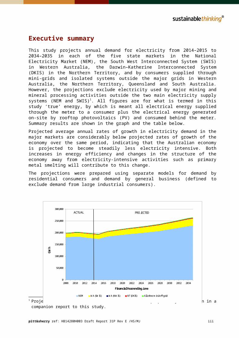
This study projects annual demand for electricity from 2014–2015 to 2034–2035 in each of the five state markets in the National Electricity Market (NEM), the South West Interconnected System (SWIS) in Western Australia, the Darwin–Katherine Interconnected System (DKIS) in the Northern Territory, and by consumers supplied through mini-grids and isolated systems outside the major grids in Western Australia, the Northern Territory, Queensland and South Australia. However, the projections exclude electricity used by major mining and mineral processing activities outside the two main electricity supply systems (NEM and SWIS)1. All figures are for what is termed in this study ‘true’ energy, by which is meant all electrical energy supplied through the meter to a consumer plus the electrical energy generated on-site by rooftop photovoltaics (PV) and consumed behind the meter. Summary results are shown in the graph and the table below.

Projected average annual rates of growth in electricity demand in the major markets are considerably below projected rates of growth of the economy over the same period, indicating that the Australian economy is projected to become steadily less electricity intensive. Both increases in energy efficiency and changes in the structure of the economy away from electricity-intensive activities such as primary metal smelting will contribute to this change.

The projections were prepared using separate models for demand by residential consumers and demand by general business (defined to exclude demand from large industrial consumers).

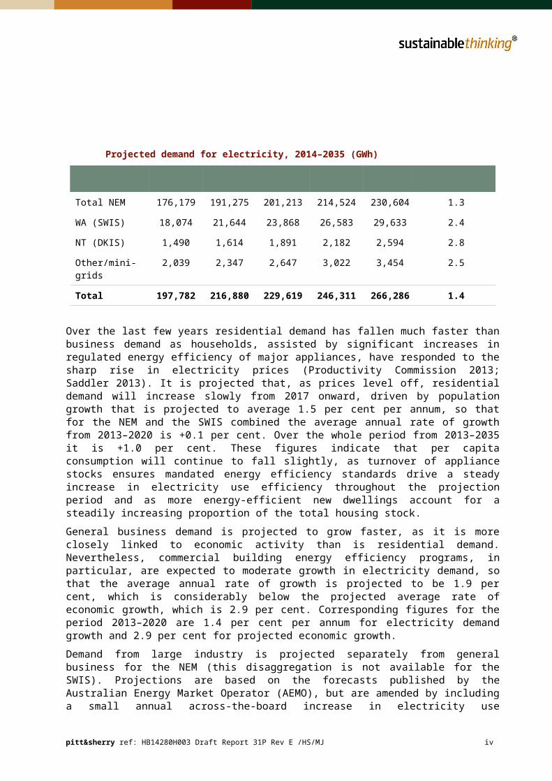
Projected demand for electricity, 2014–2035 (GWh)

1 Projections of demand from these users have been prepared by ACIL Allen in a companion report to this study.

pitt&sherry ref: HB14280H003 Draft Report 31P Rev E /HS/MJ ii

0

50,000

100,000

150,000

200,000

250,000

300,000

2008 2010 2012 2014 2016 2018 2020 2022 2024 2026 2028 2030 2032 2034

GWh

Financial Year ending June

NEM WA (SWIS) WA (NWIS) NT (DKIS) All other mini/off-grid

ACTUAL PROJECTED

Total NEM 176,179 191,275 201,213 214,524 230,604 1.3

WA (SWIS) 18,074 21,644 23,868 26,583 29,633 2.4

NT (DKIS) 1,490 1,614 1,891 2,182 2,594 2.8

Other/mini-grids 2,039 2,347 2,647 3,022 3,454 2.5

Total 197,782 216,880 229,619 246,311 266,286 1.4

Over the last few years residential demand has fallen much faster than business demand as households, assisted by significant increases in regulated energy efficiency of major appliances, have responded to the sharp rise in electricity prices (Productivity Commission 2013; Saddler 2013). It is projected that, as prices level off, residential demand will increase slowly from 2017 onward, driven by population growth that is projected to average 1.5 per cent per annum, so that for the NEM and the SWIS combined the average annual rate of growth from 2013–2020 is +0.1 per cent. Over the whole period from 2013–2035 it is +1.0 per cent. These figures indicate that per capita consumption will continue to fall slightly, as turnover of appliance stocks ensures mandated energy efficiency standards drive a steady increase in electricity use efficiency throughout the projection period and as more energy-efficient new dwellings account for a steadily increasing proportion of the total housing stock.

General business demand is projected to grow faster, as it is more closely linked to economic activity than is residential demand. Nevertheless, commercial building energy efficiency programs, in particular, are expected to moderate growth in electricity demand, so that the average annual rate of growth is projected to be 1.9 per cent, which is considerably below the projected average rate of economic growth, which is 2.9 per cent. Corresponding figures for the period 2013–2020 are 1.4 per cent per annum for electricity demand growth and 2.9 per cent for projected economic growth.

Demand from large industry is projected separately from general business for the NEM (this disaggregation is not available for the SWIS). Projections are based on the forecasts published by the Australian Energy Market Operator (AEMO), but are amended by including a small annual across-the-board increase in electricity use efficiency, based on observed trends of reported electricity use by large users in recent years. After an initial increase in Queensland, caused by the switch from gas turbine to electric motor drive for equipment used to process and transport new supplies of gas from the coal seam gasfields, currently underway, large industry demand is expected to decrease slowly over the projection period. Note that the liquefied natural gas plants themselves generate their own electricity and will not be supplied from the NEM.

The projections developed in this report have been compared with the most recent forecasts of AEMO (including the update published in December 2014), for the NEM, and the Independent Market Operator (IMO), for the SWIS. The comparison is made in terms of what the industry terms native demand, which is defined as electricity sent out to grids by major generators, plus electricity supplied by small generators other than rooftop PV. Projected native demand in the NEM is about 1.4 per cent higher than the equivalent AEMO forecast in 2020 and 4 per cent higher in 2030. For the SWIS, the projections in this study are about 6 per cent higher than the IMO estimate for 2019–2020. The main cause of these differences is the projected faster growth of general business demand in this study.

pitt&sherry ref: HB14280H003 Draft Report 31P Rev E /HS/MJ iii

1. Background and context

The Department of the Environment commissioned pitt&sherry to provide projections of demand for electrical energy in Australia from 2008–2009 to 2034–2035. Separate projections have been prepared for each of the five state markets in the National Electricity Market (NEM), for the South West Interconnected System (SWIS) and the North West Interconnected System (NWIS) in Western Australia, and the Darwin–Katherine Interconnected System (DKIS) in the Northern Territory. Projections have also been made for residential and business consumption in mini- and off-grids in Queensland, Western Australia and the Northern Territory. The projections include estimates of the impact of existing energy saving and climate change measures on Australia’s electricity demand to 2034–2035, along with broader influences on electricity demand including price and economic activity. Projections are also made of probable peak demand in each year, taking account of expected gradual increases in summer daily maximum temperatures.

The projections assume that all existing policies and measures affecting electricity demand from 2008–2009 to 2034–2035 remain in force as they are at 1 July 2014, including repeal of the carbon price, but excluding energy savings from the Direct Action Plan including the Emissions Reductions Fund. Account is taken of:

non-price drivers and barriers in demand-side profiles, including technological change and changes in social norms about how electricity is used in Australia;

changes in the structure of the Australian economy that may accelerate the decoupling of demand from economic growth;

other developments that may impact future demand for electricity in Australia.

For each of the six major state markets the project has produced estimates of:

annual demand by user type (large industrial, residential, and general commercial and industrial) (GWh);

price elasticity of demand by jurisdiction and user type;

probable annual peak demand.

pitt&sherry ref: HB14280H003 Draft Report 31P Rev E /HS/MJ 1

2. Methodology and assumptions

This section provides a detailed description of the methodology and assumptions used in the demand projections.

2.1 General approachThe key features of the approach used for this study are, first, that it uses separate spreadsheet models for residential and non-residential demand for electricity, and second, that it models demand for electricity services, not demand for electricity supplied through the meter. We briefly explain the thinking behind each of these features.

The factors influencing residential demand differ from those affecting non-residential (business) demand in several important ways. Residential demand is most directly linked to the number of households, i.e. to population, and less directly linked to the level of economic activity. For non-residential demand it is the other way round. Residential consumers have a wide array of simple behavioural options for reducing their electricity consumption in the short term, such as turning off lights, adjusting heating and cooling settings, turning on a second refrigerator only when needed, and so on. They also have many options to increase the efficiency with which they use electricity by modifying or replacing electricity-using appliances and equipment. For business consumers, by contrast, increased efficiency, rather than conservation, is their primary demand reduction option because most of their electricity consumption is directly linked to their output of goods and services.

These differences are likely to mean that residential consumers respond more quickly to changes in prices than business consumers and that residential consumption of electricity is not closely linked to the level of economic activity, whereas business consumption is closely linked.

For the purpose of this project, electricity services are defined to include electricity supplied through the meter, electricity supplied ‘behind the meter’ by rooftop PV (the combined total of which is termed ‘true’ energy in this report), and electricity not consumed at all because the same services, such as lighting, refrigeration and air-conditioning are supplied by more efficient appliances and equipment (referred to below as increased energy efficiency). When consumers decide they can meet their demand for services more cost effectively by improving energy efficiency than by purchasing additional electricity, it is rational for them to do so and increasingly likely that this will occur. It is demand for all three types of electricity services, rather than just demand for electricity supplied through the meter, which is assumed to respond to changes in electricity prices, economic activity and population.

For practical reasons, electricity services provided by increased energy efficiency are confined in this project to the efficiency gains achieved through government regulatory programs, such as Minimum Energy Performance Standards (MEPS). The models we use for residential and general business demand implicitly assume that additional efficiency improvements achieved by investments made by electricity consumers in response to higher electricity prices or other factors, over and above those mandated by government programs, occur in the future only to the extent that they have occurred in the recent past, as revealed in the process of model calibration.

In the past, ‘top down’ models of electricity demand have often used the concept of autonomous energy improvement to take account of increasing energy efficiency, whether as a result of government programs or solely as a response by electricity consumers (Graus et al. 2009; Treasury 2011). We do not apply this concept to our modelling of demand by residential and general business consumers. However, it is applied, in slightly modified form, in our analysis of a third category of consumer—large industrial or block loads. Demand for electricity by this group of consumers is, typically, largely the outcom e of discrete, large, infrequent and long-lived investment and disinvestment decisions by major electricity


consumers. Historic data suggest, however, that these consumers have been gradually increasing their electricity use efficiency over time, and our modelling projects this trend into the future. We allow for this by applying an autonomous energy efficiency coefficient to this category of electricity demand.

To the extent that the required historic data were available, the separate models as described above have been established for each of the main state grids and for various smaller grids and off-grid demand for electricity. The precise scope is as follows.

For the NEM, we constructed separate sectoral models for each of the five state markets or pools and models also for the SWIS in Western Australia, for:

residential consumption;

large industrial consumption, defined by AEMO as consumers with a maximum load of 10 MW or more;

general business consumption, which includes consumers in the commercial and services sectors of the economy, together with agriculture, and the broad range of smaller/less electricity intensive mining and manufacturing activities.

For the NWIS in Western Australia, the DKIS in the Northern Territory, and for mini- and off-grid consumption in Queensland, Western Australia and the Northern Territory our models cover:

residential consumption general business and community consumption.

For these smaller grids, as agreed with the Department, we did not model consumption by large users which, in the regions covered by these grids and other supply arrangements, are almost entirely mining and mineral processing activities. Electricity consumed by these remotely located users is included in the related electricity supply modelling by ACIL Allen, as is electricity generated and used on site, using thermal generation technologies, by industrial users connected to the NEM and the SWIS.

2.2 Key input dataProjections of population, gross state product (GSP) and real retail electricity prices in each state are key inputs to the modelling. Population projections were based on data from Treasury and the Australian Bureau of Statistics (ABS). Projections of GSP for each state were provided by the Department, based on Gross Domestic Product forecasts from Treasury. Real electricity prices were developed by ACIL Allen Consulting (2013) in a report for the (then) Department of Innovation, Industry, Climate Change, Science, Research and Tertiary Education. All projection data were provided to pitt&sherry for use in this study by the Department.

Forecast real retail electricity prices are expected to grow for the next two years, though more slowly than in the past few years, and then decrease slightly out to about 2022. Thereafter, the expectation is that prices will go up and down within fairly narrow bounds until around 2030, and then decrease slightly to the end of the projection period.

2.3 Establishing baseline historic data Modelling of the demand for electrical energy (electricity consumed through and behind the meter) starts in 2005–2006 for the NEM states and in 2007–2008 for Western Australia (SWIS only). These are the first full years for which accurate estimates of sent-out electricity are available from AEMO and Western Australia’s IMO respectively. However, as requested by the Department, results are presented from 2008–2009 onwards only, to be consistent with other sectors in the Department’s 2014 projections. Another key data source is the Australian Energy Regulator’s (AER) Network Performance


Reports for each NEM network business. These reports include estimates of annual distribution network losses, electricity supplied to residential consumers, and electricity exported to the network from rooftop PV installations, but data are only available up to 2012–2013. The models are therefore calibrated over the period from the respective starting dates to 2012–2013.

Defining the historic baselines of electricity demand, which were used to calibrate the models for each state grid, required a consistently defined time series of annual demand for electrical energy by each of the three groups of consumers used in this project, for a run of recent years. There are a number of different sources of annual time series data on electricity demand, none of which can provide the complete data required. A further complication is inconsistencies between some data series that are supposedly reporting identical data. Our approach to these challenges drew on pitt&sherry’s past experience working with the various data sets.

2.3.1 NEM state markets

Total demand on generators

The AEMO National Electricity Forecasting Reports are the most important, but not the only sources of data used for the five NEM state markets. The starting point was AEMO’s ‘operational demand’ which is identical to sent-out energy. Annual values, by state, are available for every year from 2005–2006 to 2013–2014 (which is a partial estimate) from AEMO’s 2014 National Electricity Forecasting Report data http://www.aemo.com.au/Electricity/Planning/Forecasting/National-Electricity-Forecasting-Report.

Transmission and distribution losses

AEMO’s 2014 National Electricity Forecasting Report contains estimates of annual transmission losses by state. Estimates of annual distribution network losses for each network business are found in the AER’s Network Performance Reports http://www.aer.gov.au/node/483. For each state, total distribution losses are equal to the sum of the reported losses by each network in the state (five in Victoria, three in New South Wales, two in Queensland and one each in South Australia and Tasmania). These figures were subtracted from the estimates for sent-out electricity, to obtain estimates of the quantity of electricity sourced from large central generators and supplied to final consumers.

Large users

AEMO’s 2014 National Electricity Forecasting Report publishes estimates of total annual consumption by all users with loads of 10 MW or above, which it defines as ‘large industry’. It is important to appreciate that, for all electricity consumption data, a consumer is an electricity account, which is assumed to be functionally equivalent to a site, not the company responsible for the account. Thus large businesses with facilities at many different sites will have many separate accounts, each of which will be categorised according to the consumption against the account, not consumption by the business as a whole. Defined in this way, large industry, while mainly consisting of large manufacturing and mining establishments, will also include some large commercial and service sector establishments, such as university campuses, large public hospitals and large shopping malls.


We assume that large consumers incur no distribution losses, which is only a slight over-simplification. We then have:

Electrical energy supplied to residential and general business consumers from central generators

equals electrical energy sent out from centralised generatorsminus transmission lossesminus electrical energy consumed by large industrial usersminus distribution losses.

Residential demand

For the NEM there are four separate sources of data on annual residential electricity consumption by state which could be used (details will be found in the list of references in Appendix A). These are:

1. the AER Network Performance Reports

2. the Energy Supply Association of Australia’s (ESAA) Electricity Gas Australia

3. a one-off census of network businesses covering three recent calendar years, undertaken by the ABS and published as part of Cat. No. 4670.0

4. the Bureau of Resource and Energy Economics’ (BREE) Australian Energy Statistics (2014a).

For this project it was decided to use the AER data, which present generally smooth time series for each state. The data used ran from 2005–2006 to 2012–2013. In most cases the AER data are almost identical with the ESAA data, but the latter have some discontinuities that may be caused by unspecified definitional breaks. The ABS numbers are consistently lower than AER and ESAA, while the 2014 BREE numbers (also up to 2012–2013) differ from all the others by a wide margin, and suggest trends, over time, which are also very different. They are therefore not used.

Total electrical energy supplied from distribution networks through the meter to residential consumers in each state was calculated as the sum of the quantities reported by each network business in the state.

Adjusting for rooftop PV

In recent years, residential consumers, in particular, have generated significant quantities of electricity on site by use of rooftop PV. The AER Network Performance Reports provide information on the quantities of electricity exported to each network by rooftop PV. However, these quantities do not include PV-generated electricity which is consumed ‘behind the meter’ and therefore never measured. It follows that separate estimates are required of the total quantities of electricity generated by rooftop PV in each state.

Two separate sources of estimates are available: one compiled by AEMO and published with the 2014 National Electricity Forecasting Report data, and one compiled by consultants (ACIL Allen) and provided to pitt&sherry by the Department for use in this project. The methodology used by AEMO is described in a supporting document for its 2013 National Electricity Forecasting Report (AEMO 2013), while the methodology used by ACIL Allen is described in a report provided to pitt&sherry by the Department. Both estimate installed capacity by location, month and year, using installation capacity data issued by the Clean Energy Regulator. However, they use different methods for calculating electricity generated per megawatt installed in each state. ACIL Allen uses the default output ratings used by the Clean Energy Regulator to calculate the number of certificates a system will be allocated.


There are four rating values (the rating is the number of annual megawatt-hours per installed kilowatt) based on four climate zones across Australia, making it easy to convert installed kilowatts at any location into annual megawatt-hours of electricity generated. AEMO uses a more complex approach that draws on historical Bureau of Meteorology sunlight data and other sources. The two sets of estimated historical PV electricity generation differ by amounts that are quite large for some states, notably New South Wales. Since the ACIL Allen numbers are used for projections of future PV output it was decided, in order to ensure consistency, to use this data set for the historical output also.

By subtracting the AER figures for PV exported to networks from the estimated total PV generation in each year in each state, estimates were made of behind-the-meter consumption of electricity generated by rooftop PV. A final simplifying assumption was made that, up to 2012–2013, all rooftop PV was installed on residential premises. This is reasonable, because the growth of commercial-scale rooftop PV, although likely to become very important in the years to come, has been negligible until very recently. We then have:

Total electrical energy used by residential consumers

equals electrical energy supplied through the meter from distribution networksplus output of rooftop PV consumed behind the meter.

Parenthetically, it should be noted that recent years have also seen an increase in electricity consumed behind the meter from small co/trigeneration facilities, such as those in commercial buildings and community facilities such as swimming pools. Data on the extent of this increase are limited and fragmentary, but what are available suggest that the quantities of electricity involved are both smaller and growing more slowly than electricity generated by rooftop PV. Furthermore, impending (or already observed) gas price increases are likely to dampen, rather than accelerate the rate of new installation of these co/trigeneration facilities. For this reason, excluding this source of generation will have a negligible impact on model specification.

General business demand

A further source of electricity generation is other, i.e. non-PV, generators embedded in distribution networks, such as landfill gas generators and intermittent hydro generators at irrigation storage dam outlets. AEMO terms these small non-scheduled generators (SNSGs) and has published estimates of their annual output in each state since 2005–2006. The final relationship is then:

Electrical energy used by general business consumers

equals electrical energy supplied to residential and general business consumers from central generators

minus electrical energy supplied through the meter to residential consumersplus electricity exported to the network from rooftop PVplus electricity supplied by SNSGs

On starting this project it was intended to construct separate models for the commercial and services sector (consisting, essentially, of electricity used in non-residential buildings) and a residual sector of ‘Other’ consumers, estimated by subtraction, comprising smaller manufacturing, mining and agricultural consumers. However, due to data limitations, general manufacturing, commercial and other electricity use was modelled as a single sector. In every NEM state except Tasmania, this is the largest of the three sectors, accounting for between 40 and 50 per cent of total demand. It is a smaller fraction in Tasmania, where demand is dominated by a few large industrial users. For reasons examined further below, we consider that this change will not greatly affect the quality of the models and the resulting projections.


Conclusion

The steps described in this section have been sufficient to provide estimates of historic total annual consumption of electricity by each of the three groups of consumers in the five NEM states:

residential consumers large industrial consumers general business consumers.

It should be noted that using AEMO and AER means that the numbers cover only consumers who are connected, through a local distribution network, to the NEM grid. The approach used for electricity supplied through the SWIS is described in Section 2.3.2. The approach for the small minority of consumers not connected to either the NEM or the SWIS grids is described in Section 2.3.3. The data sources that are available for both the SWIS and the other much smaller supply systems are much less detailed and comprehensive than data for the NEM, particularly outside the SWIS, which means inevitably a greater need for generalised assumptions and the exercise of professional judgment.

2.3.2 SWISThe following data were used for the SWIS:

Total sent-out energy is calculated from 30-minute sent-out data available from IMO since October 2006 (see http://www.imowa.com.au/market-reports/weekly-market-report).This data was summed for each financial year from 2007–2008 to 2013–2014.

Total transmission and distribution loss figures are contained in some annual reports of Western Power, the sole supplier of transmission and distribution services in the SWIS. For other years, the state average percentage loss figures are published each year by the ESAA in Electricity Gas Australia.

Total residential demand is taken from the 2014 edition of the ESAA’s annual Energy Gas Australia publication and is scaled down to allow for residential consumption in the NWIS and the other smaller grids operated by Horizon Power (see below).

For large industrial loads, IMO’s recently published 2014 Electricity Demand Outlook Report(see http://www.imowa.com.au/reserve-capacity/electricity-statement-of-opportunities-(esoo)) contains projections of growth in what it terms block loads, but does not contain historical figures. However, a confidential electricity consumption data set for the year to July 2008, held by pitt&sherry, makes it clear that there are no extremely large loads, comparable to aluminium smelters, in the SWIS, and almost certainly, few individual loads larger than 10 MW. We have therefore concluded that it is reasonable to model non-residential demand as a single block, without further disaggregation.

To estimate the contribution of rooftop PV to total electricity consumption, the ACIL Allen e stimates were used, as for the other states (adjusted for consumption outside the SWIS—see below). The quantity of total PV generation consumed behind the meter was estimated by applying an estimated fraction to total generation. This fraction declines year by year, because the average size of individual installations has increased year by year, and is based on the corresponding fractions calculated for the NEM states from the more detailed data described above.

2.3.3 Other gridsMuch less detailed baseline data on electricity demand is available for the Northern Territory, other small grids (Pilbara, Mount Isa, Alice Springs) and mini-grid/off-grid demand. In October 2013, BREE published a very useful report on electricity consumed outside the NEM and the SWIS; data in this report relating to small electricity consumers provided a key input to this study. The report states that


total consumption (measured as sent-out generation) in all these small supply systems was 15.8 TWh in 2011–2012, which is equivalent to 7 per cent of total Australian sent-out electricity in that year, as calculated in this study. Of the total 15.8 TWh, 12.2 TWh (equal to 77 per cent) was used by major energy and resources extraction and processing operations, such as liquefied natural gas (LNG) and metal ore processing plants. This report does not include projections of future demand for electricity from these large users. It is concerned only with the 3.6 TWh used by residential, general business and community consumers. The report provides separate data for each of the following grids and regions:

the NWIS the rest of Western Australia, i.e. outside the SWIS and the NWIS the DKIS all the rest of the Northern Territory Queensland outside the NEM South Australia outside the NEM Tasmania outside the NEM.

Separate projections have been prepared for the first five consumer groups. The final group comprises combined mini/off-grid consumption in the other four states (and is very small).

The data indicate that consumption in the DKIS is much larger than in any of the other groups (currently about 45 per cent of the total). Additional data from the Northern Territory Power and Water Corporation and the ESAA made it possible to prepare separate year-by-year estimates of recent historic residential and general business consumption in the DKIS. For the other areas, this separation was estimated by using the population figures in the BREE report in combination with assumptions about average per capita residential consumption. This was assumed to be appreciably higher than comparable averages in the NEM and the SWIS, on the basis that the tropical climate means that most households use air-conditioning almost year round and that the housing stock has, on average, lower thermal integrity than the average stock in the rest of Australia. Further expert judgement and pro-rating was used to partition total state PV generation between the main grid in each of the six states and these other mini/off-grid consumers. The final result is sets of residential and general business electricity consumption for each of the regional groups listed above.

2.4 Energy efficiency policy measures

Introduction

Since the mid-1990s Australian governments have implemented a wide array of mainly regulatory measures to increase energy efficiency. The effect of these measures has been to increase the efficiency with which electricity is used by appliances, equipment and buildings above what it would otherwise have been, i.e. above the business-as-usual efficiency level. As a result, less electricity is used to deliver the services required by consumers, such as lighting, space heating and cooling, and refrigeration. In this study we have defined the sum of the electrical energy supplied by consumption of electricity plus the reduction of energy consumption below a baseline level as a result of increased energy efficiency, as the total demand for electricity services.

For the purpose of calibrating the models, a starting year was set at 2005–2006 for the NEM states and 2007–2008 for the SWIS in Western Australia being, in each case, the first year for which complete data are available. The last year was 2012–2013, which is the most recent year with complete data. The services provided by increased energy efficiency over the calibration period are defined to equal the difference been savings in each year subsequent to 2005–2006, minus the savings in that year, which were quite modest. This means that only reductions in electricity consumption by appliances and


equipment, below the levels which would have resulted had all stocks of appliances and equipment and buildings remained at 2006 levels, are counted as supply of energy services in the calibration exercise.

Electricity savings, i.e. electricity consumption reduced, by efficiency programs, will increase steadily year by year after 2013–2014 as the historic stock of older appliances and equipment is replaced by more efficient new models and older buildings are refurbished or replaced. In addition, the annual net additions to the numbers of appliances and equipment items, and to the stock of dwellings and commercial buildings, will be more efficient and therefore use less electricity than would have been the case in the absence of energy efficiency measures. This means that, even in the absence of any new efficiency measures or increases in the stringency of existing measures, stock turnover will ensure that electricity savings increase year by year.

Energy efficiency measures were separated into those that affect residential electricity demand and those that affect general business demand. The following sections describe each in turn.

Measures affecting residential demand

Most of the electricity savings included in the study result from measures currently in force that regulate the energy use performance of appliances, equipment and buildings and support the uptake of more energy-efficient equipment. Those included in the study are as follows:

all current E3 (MEPS and labelling) measures affecting residential appliances and equipment;

Building Code of Australia (BCA) requirements (6-star) for building thermal performance in new houses and additions;

BCA requirements for lighting performance in new houses and additions to existing dwellings;

BCA requirements for water heater performance in new houses and additions;

support under the Small Renewable Energy Scheme (SRES) for accelerated uptake of solar and heat pump water heaters. Note that although the SRES is, in principle and in most practical terms, a supply-side measure, it covers these categories of equipment as ‘electricity displacement’ technologies. Electricity consumption displacement is precisely the framework used in this study to define all energy efficiency measures affecting electricity demand, and hence this measure fits perfectly alongside the other measures.

Many of these current measures have replaced measures covering the same categories of appliances, equipment and buildings at lesser levels of stringency. Many of the items purchased or installed under these now superseded measures remain in operation as part of the current stock, particularly buildings. However, these older items will continue to save energy, relative to what would have been consumed had the original regulations not been introduced, and thus will contribute to reductions in total electricity demand, relative to the demand growth trend in place prior to the introduction of energy efficiency regulations. The modelling assumes that they will be replaced with more efficient models when they reach the end of their operational life; operational lives appropriate to the particular type of equipment are used. The relevant measures and programs include the following:

BCA thermal performance requirements in force during the period since 2006, including BCA 4-star (commenced 2003 and replaced by BCA 5-star) and BCA 5-star (commenced 2008 and now replaced by BCA 6-star);

Home Insulation Program;

large-scale, low-flow showerhead roll-out programs.


Several state governments operate programs that mandate electricity retailers (directly or through contracted service providers) to undertake activities that increase residential electricity-use efficiency. These programs include:

Victorian Energy Efficiency Target (VEET) New South Wales Energy Savings Scheme South Australian Residential Energy Efficiency Scheme ACT Energy Efficiency Improvement Program.

These programs award certificates based on the total deemed savings of electricity or emissions over the future life of equipment provided or installed. Electricity retailers are required to create or purchase a specified number of such certificates each year. The annual electricity saving corresponding to a particular certificate is equal to the quantity of electricity that the certificate represents, divided by the deemed equipment life over which the quantity is calculated. The deeming life is different for each individual activity eligible to create certificates. As implied above, the savings generated extend into the future for the deemed life of the particular equipment item or activity.

Past energy savings were included in the baseline data for the purpose of model calibration, and future savings to the end of the deemed life of the various measures have been included in the projections. However, no projections were made of electricity demand reductions that might result from future actions under these four programs under the respective rules in place up to the end of 2013–2014, because it is impossible to know or even guess what mix of activities may be undertaken to meet the respective program requirements2. Furthermore, no estimate was made of demand reductions that might have been made in the past from other state programs, such as subsidised energy audits or cash subsidies for undertaking certain types of energy efficiency activities. There is little or no firm data on which to base estimates of demand reductions and uncertainty about the extent of double counting that might occur were the estimates to be made.

The very limited data available suggest that total electricity savings from these programs are likely to be small relative to the major national regulatory measures, so their exclusion is most unlikely to have a material effect on the total demand projections.

Measures affecting general business demand

A wide range of appliances, equipment and buildings used by general business are affected by energy performance regulations. Measures currently in force will continue to affect electricity demand for many years into the future, in the same way as the corresponding energy performance regulations for residential electricity use. The following current measures were included in the modelling:

all E3 (MEPS and labelling) measures affecting commercial and small industrial appliances and equipment (electric motors)

BCA requirements for the thermal performance of new and refurbished commercial buildings

BCA requirements for lighting performance in new and refurbished commercial buildings

mandatory disclosure of commercial building energy efficiency

Energy Efficiency in Government Operations

2 Because compliance is based on deemed lifetime emissions and/or energy savings and lifetimes vary between the various activities allowed under each scheme, the savings in any one year will depend on the mix of activities undertaken. This mix has changed quite radically from year to year over the life of each scheme to date, and is expected to continue to change in unpredictable ways, making the task of projecting future annual energy savings a process little better than guesswork.


National Australian Built Environment Rating System (NABERS)

New South Wales Energy Savings Scheme.

As with residential demand, we also take account of the effects on the energy performance of the stock of electricity using appliances, equipment and buildings of now superseded regulated performance standards. These include:

E3 (MEPS) requirements in force during the calibration period BCA thermal performance requirements in force during the period.

Data sources and method used to incorporate electricity savings into the modelling

Data on electricity savings resulting from the Equipment and Energy Efficiency program (E3) in all sectors was obtained from two separate sources. For a limited set of major residential appliances, the Industry Department, through the Department of the Environment, was able to provide preliminary results of the new analysis of energy savings realised through the E3 program. These results covered refrigerators, washing machines, dishwashers, residential lighting, televisions and residential air-conditioners. It uses actual, i.e. ex post, data on sales and average efficiency of the various categories of appliances and equipment, from which historic energy savings, relative to a ‘no measure’ business as usual reference, could be calculated.

For all the remaining categories of appliances and equipment used by residential, commercial and industrial electricity consumers, data contained in the report Impacts of the E3 Program by George Wilkenfeld & Associates, prepared for the government and published in 2014, was used. The Department provided, on a confidential basis, detailed year-by-year and measure-by-measure savings estimates, underlying this report. These data include both estimates of past savings and projections of future savings. The drawback of these data is that the estimates are ex ante, rather than ex post, and are therefore inherently inferior to the results of the Industry Department analysis. For reference, where results from both data sources were available, use of the Industry Department data has a relatively modest, but far from negligible effect on the projection results.

From these data the savings each year, relative to an initial year of 2005–2006, as previously described, were calculated. These savings were defined to be a component of the demand for electricity services in the relevant year. Strictly, savings should be calculated against efficiency in the year in which each measure started, but since savings were small in 2006, this would not greatly change the outcome.

Since these data are confined to an ex post analysis of historic savings, it was necessary to prepare projections of future savings from the increased efficiency of the above categories of appliances and equipment. These projections were based on the population growth figures provided for this study and took account of trends in ownership and historic rates of stock turnover of the six categories of equipment listed above, as contained in the Industry Department data. The Wilkenfeld report contains projections to 2030 of future energy savings from the various E3 measures, and these projection results were extrapolated to 2035. The complete series of combined results from the two sources was used to calculate projected demand for electricity, as described in Section 2.5.

Both sets of data on E3 program savings produced national estimates of savings from each measure. pitt&sherry allocated savings to the various states and regions in proportion to the sectoral (residential, general business) electricity consumption in each state or region in each year. For the measures affecting air-conditioning, an additional weighting factor, calculated from the population and the annual cooling degree days calculated for a weather station adjacent to the state or territory capital city, was applied.


The data source for the building energy efficiency related measures, including the BCA measures, mandatory disclosure, NABERS and Energy Efficiency in Government Operations, is a model of the Australian stock of residential buildings, by vintage, dwelling category and state, built by pitt&sherry for previous projects undertaken for the Australian Government3, which was updated and used to estimate projected savings from selected residential building efficiency measures for this project. This model includes projected future savings as well as past savings estimates.

Savings from the various state measures were calculated from data contained in annual performance reports published by the relevant state agencies.

Appendix D contains a complete list of the energy efficiency measures included in the model and of the sources of data used for each.

Calculating the annual contribution to the total supplyof electricity services of energy efficiency measures

The final outcome of these calculations is a year-by-year estimate, from 2005–2006 to 2012–2013 inclusive, of the electricity consumption savings, relative to the base year, resulting from all the measures listed above, for each consumption sector in each state or region. The measures were separated into those applying to residential electricity consumption and those applying to general commercial and industrial consumption. Since all the savings data used, from both the Industry Department and Wilkenfeld, were at the national level, it was then necessary to allocate savings between states. For most types of appliances and equipment savings, the allocation was done pro rata on the basis of each state’s share of national electricity consumption, in the residential or general commercial and industrial sectors, as applicable. For measures related to air-conditioning, an additional weighting, related to annual cooling degree days was included; this meant, for example, that Queensland and the Northern Territory were allocated a somewhat larger than pro rata share of these savings. The building measures data were already disaggregated on a state basis, so no additional allocation was needed.

These estimates for individual states, including the mini/off-grid consumers within states, were added to corresponding estimates of electricity consumption. The resultant total is called demand for electricity services.

It is important to recognise that all these projections of electricity consumption savings resulting from the various measures are based not only on the above assumptions about continuation of existing efficiency regulations, but also on explicit assumptions about ownership levels of key appliances, taking into account the potential fuel switching from gas to electric reverse-cycle air-conditioning for space heating and fuel switching from electric resistance to gas, solar and heat pumps for water heating. It is important to appreciate that the main driver for these changes, as they have progressed so far, has not been relative changes in the retail prices of electricity and gas, but rather changes in the efficiency and purchase price of the different types of equipment required (and, in the case of water heating, the subsidy to solar and heat pump systems provided through the Small Renewable Energy Scheme). The very large recent improvement in the end-use efficiency of reverse-cycle air-conditioners has been particularly important.

3 The report is no longer available on an Australian Government website, but can be found at http://www.pittsh.com.au/assets/files/CE%20Showcase/Quantitative%20Assessment%20of%20Buildings%20Measures.pdf


For the future, i.e. the period covered by the projections, savings in electricity consumption, relative to the 2006 starting date, will continue to increase and are assumed to contribute to the total demand for electricity services. The latter was estimated from the model, as described in the following pages.

2.5 Model structure and calibration

2.5.1 StructureWe postulate that for both the residential and the general business demand sectors, future demand for electricity services will be a function of the price of electricity, population and the level of economic activity.

Historic average annual population figures were obtained from ABS and a set of population projections for each state and territory was provided by the Department, sourced from Treasury.

For price, we compiled a set of historic real residential retail prices, expressed as index numbers relative to price in an initial year, for each state, by combining Australian Energy Market Commission (AEMC) estimates of absolute average annual prices with movements in the Electricity Expenditure Class in the Consumer Price Index in each state capital city, for each year from 2005–2006 to 2012–2013. Projections of future residential retail electricity prices, with no price on carbon, were provided by the Department. These price series were compiled for the Department by ACIL Allen Consulting (2013). With the removal of the carbon price (and no reinstatement), ACIL Allen projects modest thou gh steady increases in (real) electricity prices to around 2020 with, in most states, modest falls for a few years thereafter, subsequent modest increases and, finally, modest falls again after 2030.

No data were provided on average prices for electricity paid by general business consumers. This is by no means a surprise, as it is notoriously difficult to find data on prices paid by businesses, other than those with very small consumption who are paying on scheduled tariffs. The approach adopted was to assume that year-on-year relative movements in business prices are equal to the relative movements in residential prices, even though absolute levels of residential and business prices are likely to be different. Pragmatically, since no great changes in electricity prices are expected, price is unlikely to be an important driver of demand for electricity, meaning that this simplifying assumption should not have a major effect on the results.

For economic activity, the parameter used is real GSP. Historic values were again obtained from ABS publications and projections were provided by the Department, based on Treasury and ABS forecasts. For model testing and calibration purposes, some use was also made of value added by economic sector components of GSP.

In specifying the form of models, pitt&sherry has placed particular emphasis on the implications of the extremely large and rapid changes currently being experienced by the electricity supply industry. Changes in the cost and technical performance of important classes of electricity using equipment, similar changes in small-scale generation technologies, particularly PV, and apparent changes in the preferences and behaviour of electricity consumers are all likely to mean that very precisely calculated relationships between prices, income and demand in the past may not hold with the same precision in the future. Furthermore, the size and duration of the electricity price changes over the last few years are, on the one hand, historically unprecedented, and, on the other hand, now coming to an end. These considerations also mean that other drivers, such as weather (measured heating and cooling degree days) are likely to have a different (and in this case smaller) impact than in the past, as air-conditioning systems become more efficient and buildings better insulated and sealed. The fact that electricity demand data of good quality, as described in the preceding pages, are only available for a short series of


past years, has also been a very important consideration.

The approach taken was not to construct and calibrate complex econometric models with precisely defined uncertainty ranges, but rather to specify simple models and seek to calibrate them across the various state data series with the aim of obtaining elasticity values that are broadly consistent across the country. All models are calibrated using annual data, as already described, from 2005–2006 to 2012–2013 inclusive for the NEM states and 2007–2008 to 2012–2013 inclusive for the SWIS.

2.5.2 Calibration

Residential sector model

For the residential sector, the average number of persons (total population) per residential customer was extremely constant in each state over the whole calibration period. This ratio was taken as a proxy for household size and assumed to remain constant over the projection period. The number of households is therefore proportional to population, and demand is modelled on a per capita basis. Separate calibration for each state yielded a good fit of in each case to a simple model in which demand for electricity services is determined by the product of a price response component and a ‘behavioural multiplier’ component, which may be thought of as a proxy for the continued slow growth in the average volume of electricity using equipment and appliances in households across the country. The parameter values are:

a price elasticity value of –0.3, and a ‘behavioural multiplier’ value of 1.005.

A price elasticity of –0.3 means that if the price of electricity increases by, say, 10 per cent from one year to the next, demand for electricity services can be expected to fall by 3 per cent, all else being equal. The ‘behavioural multiplier’ may be thought of as an alternative to an income effect. We have expressed it in this form because we consider that at this stage of economic development the continued take-up of new uses for electricity is much less a function of increasing household income than it is of the increasing availability and decreasing real cost of electrical appliances and equipment.

This model generally fits well with the observed changes in demand for electricity services in each state over the calibration period, with the important proviso that price elasticity is zero up to 2010 and –0.3 thereafter4.

General business model

For the reasons explained in Section 2.1, the expectation is that the most important driver of electricity demand from this consumer sector will be the level of output of goods and services, for which the most appropriate measure is GSP. Looking below the level of total GSP, the economic sectors responsible for most of the electricity demand under consideration can be separated into manufacturing and mining on the one hand (still accounting for much of the demand, even though the very large individual users are modelled separately), and the service sector on the other hand. When defined in terms of ANZSIC, the service sector consists of a number of separate Divisions, which together constitute around two-thirds of total economic activity, nationally and in each state. However, on average, the services sector is much less electricity intensive than either manufacturing or mining; in total it accounts for between 25 and 30 per cent of total electrical energy demand.

4 The most likely explanation for this observed change in the behaviour of residential electricity consumers is that first large electricity price increases occurred only shortly before 2010, and this was the first year in which the size of electricity price increases, and the contribution to these increase of government policies, first became a topic of wide public comment and debate.



If trends of the past few decades continue, it is likely that economic activity by the manufacturing and mining sectors will grow more slowly than commercial and service sector economic activity. Since the commercial and services sectors account for the great majority of GSP, the relativities would mean that the modelling approach tends to over-estimate future electricity demand. For this reason, it would be desirable to be able to separate general business demand from the commercial and services sectors of the economy from demand arising from other sectors. Unfortunately, as explained in Section 2.3.1, the electricity demand data needed to construct rigorous models on this basis are not available. For some states, a model that partitioned economic activity between services and manufacturing/mining was found to give a better fit than a version that used total GSP as a driver, which is what would be expected, given the differing electricity intensities of the two sectoral groups.

Overall, however, a simpler model expressing demand for electricity services by this whole consumption sector as a function of economic activity and electricity price was found to give a generally good fit to the historic demand figures in each state. Furthermore, for the purposes of projecting future demand, the more refined version is of little value, because projections of future GSP are available only at the whole economy level, not disaggregated into separate economic sectors. Demand for electricity services is therefore expressed as a function of price and GSP.

It was found that a price elasticity value of –0.1 gave a good fit with historic data for all states.

For income, i.e. GSP, elasticity, it was found that states divided into two groups. For New South Wales, Queensland and Tasmania, a value of 0.95 gives the best fit, while for Victoria, South Australia and Western Australia a value of 0.75 is best. The reason or reasons for this difference between states are not immediately obvious. A possible explanation may be the differences between states in the shares of the more and less electricity-intensive economic activities accounting for general business demand for electricity. While in every state, the less electricity-intensive activities (meaning, in general, most service sector activities) account for the majority of GSP, the proportion varies somewhat between states. In states where this proportion is somewhat lower, and the more electricity-intensive industries account for a large share of GSP, demand should be more responsive to changes in GSP, all else being equal, than in states where more electricity intensive activities make a smaller contribution to GSP. Unfortunately, available data are not sufficient to allow this hypothesis to be tested.

Overall, of course, income elasticities of less than 1 mean that the electricity intensity of an increase in economic activity is, on average, less than the average electricity intensity of total economic activity. This means that over time the economy as a whole will become gradually less electricity intensive. Nevertheless, the elasticity values mean that, in the absence of further large price increases, future economic growth will lead to growth in demand for electricity services.

Large industry

Projections of demand from large industry are based on the 2014 forecasts from AEMO’s 2014 National Electricity Forecasting Report, for the NEM states, and on the IMO’s 2014 Demand Outlook for the SWIS, using the Medium or Expected case in all instances. The two organisations prepare estimates of future demand from this group by directly asking the relatively small number of electricity consumers involved to advise what they expect their future demand may be. These expectations will in all cases be affected both by possible plant closures or restructuring and also by major new investments. This means that they are commercially sensitive, and therefore both AEMO and IMO publish the projections as aggregates only, with certain exceptions where changes are already publicly known. Changes in electricity demand from this group are mainly driven by discrete investment/disinvestment decisions about individual sites, and in the short to medium term are not greatly influenced by changes in electricity prices.


AEMO expects a significant step increase in demand in Queensland caused by the major coal seam gas producers switching to electric drive for extensions to their planned very extensive network of compressors in their respective networks of gathering pipelines (Powerlink 2014). This increase in demand is assumed to remain for the whole projection period. The Queensland transmission network service provider, Powerlink, is well advanced with building the required transmission infrastructure to meet this demand. The demand increase will roughly coincide with the commissioning of the LNG plants which the gas fields supply, but is not at the LNG plants: they will all generate their own electricity requirements on site and will not be supplied from the grid.

AEMO projects very little growth in demand from other large users. In November 2014 AEMO published new large industry demand projections for Queensland and Tasmania, incorporating small changes to the previously published figures. Allowance has also been made for a very large new load in Queensland, not anticipated by AEMO, which appeared in late October 2014. IMO also expects only a modest growth in demand from unspecified large users, which it terms block loads, in the SWIS. This is in marked contrast to a few years ago when very considerable growth in demand was expected from new mineral processing projects, especially magnetite, in the northern part of the area covered by the SWIS.

Examination of the most recent report by BREE (2014b) on potential new resources and energy projects confirmed that the overwhelming majority of new projects were in locations beyond the current major grids, and so would not affect demand within the grids. It is assumed that there will be no further closures among the four remaining aluminium smelters (AEMO included the possibility of a further 50 per cent fall in demand from aluminium smelters in its Low scenario, followed by closures for each smelter once its existing electricity contract expires, but not in its Medium scenario).

Examination of five years of NGERS data on Scope 2 emissions by major emitters demonstrates, on average, a consistent and persistent gradual fall in emissions, faster than can be explained by reductions in the emissions intensity of electricity. National accounts data on value added by major mining and electricity intensive sectors of the economy do not indicate an equivalent decline in output, and neither do commodity production statistics show a decline.

We therefore concluded that the reduction in emissions is consistent with gradual increases in the productivity of electricity used by the relevant industries, as indicated, for example, by statistics from the Energy Efficiency Opportunities program. It was also assumed that the Australian economy will continue its secular structural shift away from electricity intensive materials processing industries, meaning that there is no over-arching reason to expect an upsurge in economic activity by these sectors of the economy. Accordingly, pitt&sherry amended the AEMO projections for demand from large electricity users by applying an across the board reduction in electricity demand of 0.8 per cent per annum to the AEMO forecasts for electrical energy demand by this sector5. As a result, for example, by 2019–2020, large industrial demand across the NEM is projected to be 47,400 GWh, compared with an equivalent AEMO figure of 49,139 GWh.

Estimates of future demand for electricity by large users located beyond the six main state distribution networks have been prepared by ACIL Allen Consulting.

5 A range of values can be found in the relevant economic literature; see for example, Graus et al. 2009; Treasury 2011; Che & Pham 2012.


2.6 Calculating total final consumption of electricity Future annual demand for electricity services was calculated for each of the three major demand sectors in each state, using the various models described above, which link demand to future population, GSP and electricity prices.

The estimated future electricity demand reductions resulting from the various energy efficiency measures in the residential and general business sectors were then subtracted from the respective year-by-year projections of demand for electricity services, to give demand for electrical energy.

Demand for electrical energy

equals demand for electricity servicesminus electricity savings from efficiency measures.

It is interesting to note that use of the newly available Industry Department data on past electricity savings had a somewhat counter-intuitive effect on projections of future demand for electricity. Compared with the Wilkenfeld data initially used, the new data, for the measures for which it was available, somewhat increased the savings attributable to the measures during the calibration period. This was mainly because it indicated a faster replacement of old stock than assumed in the Wilkenfeld analysis. The savings from each individual measure are determined by the average efficiency improvement when an existing stock item is replaced with a new item which meets the new regulated efficiency level, multiplied by the stock numbers. Hence more stock replaced in earlier years means more savings realised and fewer to come from the total potential, which is a function of the total number of items in the stock, a value for which there is broad agreement between two sets of results across all appliance types. In other words, the faster turnover in the immediate past means that are fewer energy savings to be realised from the existing regulatory settings in the years to come. Consequently, demand for electricity services was found to have been growing somewhat faster than originally thought, and was higher in last full calibration year (2012–2013). This in turn meant that projected future levels of electricity services were also somewhat higher, and that, in addition, future savings were somewhat less, as more had already been realised prior to 2013–2014. Consequently, demand for ‘true’ electricity was projected to grow somewhat faster than it had been in the original model runs.

In this study, the estimates of demand for electrical energy, net of savings from efficiency measures, are termed ‘true’ demand for electricity, as the figures include both electricity supplied through the meter from all sources of generation, i.e. central and distributed, and electricity supplied by rooftop PV and consumed behind the meter. This definition of electricity demand differs from those normally used, which in most cases refer only to electricity supplied through the meter, i.e. excluding behind-the-meter PV consumption. Year-by-year projections of ‘true’ electricity demand from the residential and general business sectors were added to the projected large industrial demand for in each state to obtain projections of total ‘true’ electricity demand for each state.

Note that it is not possible to prepare projections of demand for electricity supplied through the meter because this would require behind-the-meter consumption from rooftop PV to be subtracted from ‘true’ electricity demand. While, as previously described, there are a number of projections of total future supply from rooftop PV, there are no projections of the share of this total supply which may be consumed behind the meter (and no sound basis for preparing such projections).


However, it is possible in principle to prepare soundly based projections of demand for sent-out electricity, i.e. electrical energy supplied by large (grid connected) generators, which is defined as follows.

Demand for sent out electricity

equals ‘true’ demand for electricityminus total electricity generated by rooftop PV (including both behind-the-meter consumption

and generation exported to the networks)minus electricity supplied to networks by other embedded generators (SNSGs)plus distribution lossesplus transmission losses.

AEMO has prepared forecasts of future supply by SNSGs, but there are no corresponding figures for the SWIS from IMO. For this study, therefore, projections have been made of what AEMO terms native demand, which is equal to sent-out demand plus energy supplied by SNSGs, but excluding supply from rooftop PV. This approach makes it possible to present results for the five NEM states and the SWIS on a consistent basis, while also allowing direct comparison of recent projections by both AEMO. Thus:

Native demand for electricity

equals ‘true’ demand for electricityminus total electricity generated by rooftop PV (including both behind-the-meter consumption

and generation exported to the networks)plus distribution lossesplus transmission losses.

Sources for the three additional sets of projected data are as follows.

Total electricity supplied by rooftop PV is equal to the projected values for each state prepared by ACIL Allen Consulting, as described above and provided for this project by the Department.

Transmission and distribution losses, in total, in each state system are assumed to be the same percentage of demand by final consumers net of PV as in 2013–2014. These percentages were 6.6 per cent in New South Wales, 8.3 per cent in Victoria, 7.0 per cent in Queensland, 8.2 per cent in South Australia, 5.3 per cent in Tasmania, and 6.3 per cent in the SWIS. These are rather sweeping assumptions, but the historic record provides no firm basis for projecting the future, as in most states it shows considerable year on year volatility, with no obvious relationship to possible causal factors, such as the peakiness of the annual load duration curve.

2.7 Sensitivity analysisThe sensitivity of the results to varying three different input assumptions was tested.

Growth in GSP is the most important driver of future demand from general business, the largest of the three sectors into which electricity demand was separated in this study. Generalised income growth also has a more modest influence on residential demand. Sensitivity to income growth rates was tested by modelling future demand with rates of GSP growth in each state 25 per cent higher and 25 per cent lower than in the ‘central’ projection. A further test was undertaken by setting the income elasticity of demand for the three states in which high elasticity values were found in the course of calibration—Victoria, South Australia and Western Australia—at the same lower level as found in the other three states.


Both residential and general business demand are also sensitive to changes in the real price of electricity (Productivity Commission 2013; Saddler 2013). The ‘central’ projection case is that, following the very large increase of recent years, changes in prices from now on, whether up or down, will be small. Our assessment is that further significant increases in real electricity prices are extremely unlikely. However, reductions in prices are somewhat more likely. The sensitivity of demand to lower electricity prices was therefore tested by setting prices to fall progressively over the ten years from 2015–2024 by 2 per cent of the ‘central’ case price for that year in each state. That is, prices are 2 per cent below the ‘central’ level in 2015, 4 per cent below in 2016, and so on, up to 20 per cent below in 2024. Thereafter prices remain at 20 per cent below the ‘central’ level.

Plausible combinations of the changes described above were combined to develop a complete envelope of plausible projection results. In summary, the options tested were as follows:

higher income growth

lower income growth

lower income elasticity of general business demand in Victoria, South Australia and Western Australia

lower income growth and lower income elasticity in these three states, combined (termed the ‘super low’ option)

lower electricity prices

higher income growth and lower electricity prices combined (termed the ‘super high’ option).

A separate sensitivity analysis, exploring the most likely effect of higher gas prices in eastern Australia, was also undertaken. Gas prices are already rising strongly in eastern Australia, with more price rises expected over the next three to four years as domestic prices realign with international prices, due to the construction of an increasing number of LNG facilities on the east coast. Gas prices have already risen significantly in Western Australia in recent years for similar reasons (exacerbated by tightening pipeline spare capacity). Since gas and electricity are substitutes in certain end-uses, and with real electricity prices expected to fall while real gas prices rise, it is likely that substitution will occur. However, it is not sufficient to consider price relativities alone. In particular, consideration must also be given to real technical options for electricity to displace gas which both reduce the energy input cost and also do not require excessively high costs to replace the energy using equipment. Options are limited in most general business applications, where gas is used in boilers, ovens, kilns and the like to produce heat. Separate economic analysis undertaken by pitt&sherry for various clients shows that, in most locations and most residential space heating demand situations across Australia, modern heat pumps (reverse-cycle air-conditioners) have relatively modest capital costs and lower operating costs than gas heaters. We have therefore assessed that this is where replacement of gas by electricity is most likely to occur.

The sensitivity analysis assessed the potential extent of residential consumption of gas for space heating to be displaced by electricity, using detailed state-by-state data on residential energy demand contained in the results of a major consumer survey by the ABS (2014). Modern residential reverse-cycle air-conditioners have a coefficient of performance (sometimes termed energy efficiency ratio) of 4 or more, meaning that they can supply four or more units of useful heat energy for every one unit of electrical energy consumed. By contrast, a well maintained standard gas heater used in Australia would be unlikely to be able to deliver more than 0.8 units of useful heat for every one unit of gas consumed, most of the remaining energy being lost in flue gases. Hence, as a generalisation, replacing 1 GJ of gas used in a space heater with a reverse-cycle air-conditioner providing the same amount of useful heat output will result in the additional consumption of 0.8/4 = 0.2 GJ, equal to 56 kWh, of electricity.


2.8 Peak demand Annual peak demand is related to total electrical energy used by final consumers, but is also affected by a number of other factors, including:

maximum daily temperature on the peak day

whether that day is a ‘one-off’ or is the last day of a heatwave of several days duration

reductions in demand for electrical energy arising from increased efficiency of air-conditioners and the increased thermal efficiency of building envelopes

output from PV at relevant times of the day.

Differences between states in climate and economic structure mean that the relationship of peak demand to total energy consumption also differs. The annual peak in all states except Tasmania now occurs in summer, although until recently New South Wales peaks occurred alternately in successive summers and winters against a background of an almost fixed relationship between energy demand and peak. Until recently, increasing ownership and use of air-conditioners, particularly by residential consumers, caused annual system peak, weather corrected, to increase faster than total annual energy demand, i.e. the average system load factor was decreasing. However, this trend appears to have saturated over the last few years; both AEMO and IMO project annual P50 system load factor to remain virtually constant over coming years. (P50 means the value which has a probability of 50 per cent of being below, and a 50 per cent probability of being above, the actual value, in each year.)

Detailed examination of daily electricity consumption patterns in both the NEM and the SWIS makes it clear that the relationship between summer peak and daily maximum temperature is a very close one. For each state, historic data was collected on maximum demand on a selection of the hottest working days each year since 2006 and the maximum temperature on the relevant day. A single temperature parameter was used for each state, taken from Bureau of Meteorology historical records of Climate Data Online for a weather station close to and inland from the state capital, e.g. the airport or another airfield in most cases. These analyses were used to establish relationships for each state which express peak demand as a function of annual energy demand and maximum temperature on the day.

The functional form of the relationship differs between states. The individual state equations are shown in the box below. It can be seen that in all states, the larger part of peak demand is a simple linear function of, i.e. directly proportional to, total annual energy demand. Historic annual peak demand in Queensland can be adequately represented by this simple relationship, but in other states more complex relationships, with temperature dependent components, are required.

In South Australia, it was found that working day maximum demand is directly proportional to energy demand for maximum temperatures up to 27 deg. C; at higher daily maximum temperatures a further linear increase in maximum demand occurs, equal to just over 5 per cent of demand at 27 deg. per degree above 27 deg. C. In Victoria, a similar relationship was found, but the temperature dependent increase starts at 23 deg. C and is equal to just over 3 per cent of peak at that temperature per degree increase in daily maximum temperature. However, on the hottest days, there is an additional small multiplier based on the number of preceding days with maximum temperatures above 40 deg. In New South Wales, daily peak demand is also affected by maximum temperature, but there is a two-part relationship. Daily peaks increase modestly for each degree that the daily maximum is above 23 deg. C, and more rapidly with each degree above 35 deg. C. A similar relationship is found for the SWIS, but with the functional break at 31 deg. C rather than 35. Daily peaks are largely driven by residential demand and these differences between states in the functional form of the relationship between maximum temperature and peak demand can be plausibly explained by differences in climate and the use of residential air-conditioning.


Equations relating peak demand (in MW) to energy demand and maximum temperature

NSW peak demand = E x (0.135 + (0.002 x 12) + (0.004 x (T – 34)))

Vic. peak demand = E x (0.125 + (0.0042 x (T – 23)) x (1 + (0.05 x n)))

Qld peak demand = E x 0.179

SA peak demand = E x (0.130 + (0.007 x (T – 27))

SWIS peak demand = E x (0.125 + (0.005 x 8) + (0.006 x (T – 31)))

Where:

E = Annual peak demand for electrical energy in MWT = Annual maximum temperature in deg. Cn = Number of preceding days with maximum temperature above 40 deg. C

The box below shows the equations used for each state. The various numbers in the equations are constants, and the three variables are defined at the bottom.

These relationships are important because it is expected that climate change will cause a gradual increase in the average annual maximum temperatures in every state. For this project we used the results of the Climate Change in Australia study by CSIRO and the Bureau of Meteorology (CSIRO 2007) to determine the extent of increases in maximum temperatures. Under the study’s A1B (medium emissions) scenario, the P50 temperature increase average annual temperature by 2030 in all state capitals is 0.8 deg. C, relative to a historic reference period of 1980–1999.

Further analysis of the data shows that this increase applies equally to average daily maxima and average daily minima. We assumed that this would be the average increase between 2014 and 2030, i.e. we assumed that there is so far been no increase in average temperatures relative to the reference period, which will slightly overstate the size of the increase between now and 2014. On the basis of this increase to 2050, P50 annual maximum temperatures for each state capital were calculated and extrapolated to 2035. These temperatures were then combined with projected annual energy demand for each state, to calculate P50 annual peak, using the relationships for each state described above.

A further adjustment was then made to allow for the potential effect of increased efficiency of residential air-conditioners on peak demand. For most appliances and equipment, the reduction in annual energy demand caused by increased energy efficiency is assumed to have a directly proportional impact in reducing peak demand. In other words, appliances and equipment are implicitly assumed to have, on average, the same load factor as the system as a whole. This assumption is clearly not valid for air-conditioners, which in southern Australia usually operate only in the summer months and often only on hotter days. This means that annual peak saving will be quite large relative to total annual energy saving, a relationship expressed by the reciprocal of this ratio, i.e. peak saving divided by annual energy saving, which is defined as the Conservation Load Factor or CLF (Koomey 1990). For Queensland, South Australia and the SWIS, a CLF value of 0.1 is used. This is at the upper (and therefore conservative) end of the generally accepted range of 0.01 to 0.1, but is appropriate for these states, which have relatively long hot summers (or in the case of Queensland a sub-tropical/tropical climate) resulting in a large total of annual cooling degree days, implying a large number of operating air-conditioner hours each year.


New South Wales and Victoria have considerably smaller numbers of annual cooling degree days, and a CLF value of 0.05 is used. These values were used to calculate the reductions in peak demand corresponding to the annual reductions in annual electricity consumption from the two residential air-conditioning measures included among the E3 measures, as described in Section 2.4. These additional peak savings were subtracted from each of the P50 annual peak estimates calculated from the temperature data, to obtain final projections of peak demand for each mainland NEM state and the SWIS.

Finally, it is important to note that all estimates of peak demand relate to our projections of ‘true’ electricity consumption. In other words, the peaks we have calculated are ‘true’ peak demand for electricity, not network peaks. No account has been taken of the contribution of small scale PV to peak demand on electricity networks. It is apparent that in at least some states in the last couple of years, PV output has had the effect of shifting the time and reducing the size of network peaks. However, this relationship is complex, varies between states, and depends to some extent on time of year and to a large extent on the hour to hour weather on the individual day of peak demand. It also depends, of course, on the proportion of total PV output which is supplied behind the meter.


3. Projection results

3.1 Results by state/regionProjected demand for what we have termed ‘true’ demand for electrical energy, including electricity supplied from rooftop PV behind the meter, as well as all energy supplied through the meter from the distribution network, is shown for baseline assumptions in Figure 1. The data excludes major industrial demand supplied outside the six state systems and the Northern Territory DKIS; this will be a small fraction of total demand. Corresponding numerical values for selected years are shown in Table 1 for each of the five state markets in the NEM, the Western Australian SWIS and the DKIS.

0

50,000

100,000

150,000

200,000

250,000

300,000

2008 2010 2012 2014 2016 2018 2020 2022 2024 2026 2028 2030 2032 2034

GWh


NEM WA (SWIS) WA (NWIS) NT (DKIS) All other mini/off-grid

ACTUAL PROJECTED

Figure 1 Projected annual demand for ‘true’ energy from allAustralian electricity supply systems (GWh)

Presenting the results in this format mainly serves to show that the Australian total is dominated by demand in the NEM and the SWIS. It also shows that total demand is projected to fall again in 2014–2015, and to then resume growing in absolute terms. The projected average annual rate of growth of demand in the NEM for the whole period from 2013–2014 to 2034–2035 is 1.3 per cent. While greater than demand growth which occurred from about 2003–2010, and of course the decline in demand since 2010, 1.3 per cent is considerably less than the long term historic rate of growth prior to 2003.

Projections for the five state regions within the NEM and the SWIS are shown in Figure 2 and also in Table 1. These data exclude electricity consumed within state borders, but not within the major grids, i.e. the mini/off-grid demand shown in Figure 1.



0

10,000

20,000

30,000

40,000

50,000

60,000

70,000

80,000

2006 2008 2010 2012 2014 2016 2018 2020 2022 2024 2026 2028 2030 2032 2034

GWh


NSW + ACT Victoria Queensland SA Tasmania WA (SWIS)

ACTUAL PROJECTED

Figure 2 Projected annual demand for ‘true’ energy (GWh)

Table 1 Projected ‘true’ annual demand for electrical energy (GWh)

NSW & ACT 63,813 65,002 68,232 72,768 78,396 1.0

Vic. 43,440 42,707 46,298 50,486 55,754 1.2

Qld 46,290 61,133 64,149 68,459 70,903 2.2

SA 12,597 12,525 12,653 12,968 13,720 0.4

Tas. 10,039 9,908 9,881 9,843 9,830 - 0.1

NEM total 176,179 191,275 201,213 214,524 230,604 1.3

WA (SWIS) 18,074 21,644 23,868 26,583 29,633 2.4

NT (DKIS) 1,490 1,614 1,891 2,182 2,594 2.7

Other/mini-grids* 2,039 2,347 2,647 3,022 3,454 2.5

Total 197,782 216,880 229,619 246,311 266,286 1.4

* Sent-out energy, not ‘true’ energy demand


Differences between states can be attributed to specific discrete changes in demand by large industrial users in some states and to differences between states in projected rates of growth of population and GSP. Particular points include the following.

In New South Wales demand fell much faster in the recent past than in other states, because of both the closure of the Kurri Kurri aluminium smelter (October 2012) and a much larger fall in residential demand than in other states. In the future, modest growth in both residential and general business demand are projected, but increased electricity use efficiency is projected to bring a slight fall in large industry demand.

In Victoria, a corresponding fall in demand has occurred in 2014–2015 because of the Point Henry aluminium smelter closure (August 2014). Projected demand growth in subsequent years is attributable to relatively high population growth and to the fact that analysis of historic demand by general business shows a higher responsiveness to growth in GSP than in some other states.

In Queensland, the marked increase in demand over the next few years is largely caused by the large jump in demand from the coal seam gas industry, as previously described. Continuing projected high population and GSP growth also contributes to strong growth in demand for electricity.

In South Australia, GSP is expected to grow more slowly than in other states and consequently general business electricity demand is projected to also grow more slowly. AEMO projects no increase in large industry demand, which means that, when the effect of modest efficiency improvement is included, demand from this sector decreases. Residential demand is also projected to fall slightly over the projection period, as the effect of increased electricity use efficiency outweighs the effect on demand of population growth below the national average rate.

In Tasmania, total state demand is dominated by four large industrial users, accounting for well over half of total demand. The assumed small but steady increase in electricity use efficiency by all large users, together with population growth less than the average national rate means that overall a small decrease in electricity demand is expected.

In Western Australia (SWIS only), both population and GSP are projected to grow faster than the national average, leading to above average rates of growth in total demand. However, the relationship between GSP and demand for electricity in the SWIS is complicated, because a high proportion of GSP in recent years has been linked to mining and gas production activity, most of which is located outside the SWIS, and many of the major new mineral resource projects, such as new LNG production, will also be outside the SWIS area. Electricity demand projections for the SWIS may therefore be subject to greater uncertainties than projections for other states.

3.2 Results by demand sectorAs Figure 2 shows, there are quite significant differences between states in projected growth of electricity demand. These differences can mostly be explained by differences in how the separate demand sectors are expected to change in the various states. The combined results for the NEM and the SWIS, disaggregated by demand sector, are shown in Figures 3 and 4, and Table 2. Key features of and differences between the demand sectors across the various states are described in turn.


Figure 3 Projected annual ‘true’ energy demand in the NEM by demand sector (GWh)

Figure 4 Projected annual ‘true’ energy demand in the SWIS by demand sector (GWh)

Table 2 Projected annual ‘true’ energy demand by demand sector in the NEM and the SWIS (GWh)


0

5,000

10,000

15,000

20,000

25,000

2006 2008 2010 2012 2014 2016 2018 2020 2022 2024 2026 2028 2030 2032 2034

GWh

Financial Year ending JuneResidential All business

ACTUAL PROJECTED

0

20,000

40,000

60,000

80,000

100,000

120,000

140,000

2006 2008 2010 2012 2014 2016 2018 2020 2022 2024 2026 2028 2030 2032 2034

GWh

Financial Year ending JuneResidential Large industry General business

ACTUAL PROJECTED

Residential 50,766 51,264 54,343 59,020 62,894

General business 82,718 89,018 97,184 107,008 120,464

Large industry 44,731 50,993 49,686 48,497 47,246

NEM total 178,215 191,275 201,213 214,524 230,604

Residential 5,283 5,265 5,737 6,540 7,361

All business, includinglarge industry

12,135 16,378 18,132 20.043 22,272

WA (SWIS) Total 17,418 21,644 23,868 26,583 29,633

Large industry

Large industry demand in the NEM initially falls because of the closure of the Kurri Kurri aluminium smelter in New South Wales during the 2012 calendar year and the Point Henry aluminium smelter in Victoria from August 2014. It then grows strongly, from 2015–2018, because of the surge in demand for coal seam gas field compression in Queensland, as described earlier. This demand derives from the decision by two of the three consortia developing LNG export projects based on coal seam gas to convert their gas field operations from gas engine drive to electric motor drive. Because coal seam gas production requires far more individual wells, spread over a much wider geographical area than conventional natural gas production, it requires much larger use of energy in compressors to move the gas along pipelines. Powerlink, the Queensland transmission network service provider, is making major extension to the Queensland electricity grid to meet this demand. It has estimated than this demand may increase total Queensland demand by 17 per cent between 2014–2015 and 2017–2018 (Powerlink 2014). All of this increase will come from the gas field region; Powerlink projects a modest fall in total demand for electricity over the same period across all other regions in the state. Note that, while this new demand for electricity is coming from the LNG consortia, the demand is not at their LNG plants, but at their gas fields. The LNG plants themselves will be entirely self-sufficient for electricity and will not draw on NEM supply (Jacobs SKM 2014).

No further assumptions are made about either establishment of major new sources of electricity demand or closure of existing sources. Consequently, demand in all states is projected to slowly decline from 2020 onward, driven by the assumption of a gradual increase in the average efficiency of electricity use. For the SWIS, there is no projection of demand by large industry (termed blockloads by IMO) as a separate sector. All industrial demand is included within General business, but an adjustment is made for a modest increase in blockload demand specified by IMO in its most recent forecasting report.


Residential

Since 2010 there have been sharp falls in total residential demand, even when demand is adjusted to include both electricity supplied through the meter and electricity from rooftop PV consumed behind the meter. These falls are projected to end by 2016, as consumers complete their adjustments to the large price rises of recent years, and further price increases come to an end. On a per capita basis, residential demand grows slowly from 2018 onward. The main driver of increases in demand is population growth, which is slower than growth in GSP. The assumption of a modest underlying growth in the ownership of electricity using appliances and equipment also contributes to demand growth. However, the effect of both these factors is substantially offset by the steady spread of more efficient appliances, equipment and buildings throughout the residential sector. In addition, the contribution of demand reductions from the various energy efficiency measures has a relatively larger impact on residential demand than on the general business sector. Overall, this means that growth in residential demand is substantially slower than growth in GSP.

General business

General business is the source of not only the largest share of total electricity demand, but also the most rapid growth expected in the years to come. This reflects the strong relationship between total economic activity, as measured by GSP, and demand for electricity, although in the NEM, at an average rate of 1.8 per cent per annum, growth in electricity demand is considerably slower than projected growth in combined GSP of the five states (including the Australian Capital Territory), which is 2.8 per cent per annum.

In the NEM, demand is projected to increase by 36 per cent from 2013–2035, while total electricity demand growth over the same period is projected to be 21 per cent. As a result, general business demand increases from 46 per cent of total demand in 2013 to 52 per cent in 2035, meaning that, overall, the rate of growth of demand by this sector is the largest determinant of how fast total demand for electricity is projected to grow. In the recent past, as electricity prices rapidly increased, general business demand has been roughly constant, apart from a one-year blip down at the height of the financial crisis. As described in Section 2.2, it is expected that further electricity price rises will be modest. As a result, demand for electricity services grows considerably faster than can be offset by increased efficiency of electricity use through the current regulatory measures and other programs.

In the SWIS, general business demand growth is high, both because of projected rapid growth in GSP, as noted above, and also because analysis of past demand showed a closer relationship of electricity demand to GSP than in the NEM states, other than Victoria.

3.3 Comparison of results with AEMO and IMO projectionsAll results presented to this point have been for what is termed in this report ‘true’ energy demand, meaning all electricity supplied to consumers through the meter, plus electricity generated by rooftop PV and consumed behind the meter. This is not a concept used by either AEMO or IMO. The most appropriate basis for comparison is native demand for electrical energy, which is used by both organisations. In order to convert the projections of ‘true’ energy developed in this report to native energy, it is necessary to subtract projected supply from rooftop PV and add estimates of future transmission and distribution losses to the ‘true’ energy projections.


The results of the comparison prepared in this way are shown in Table 3, using the most recent (December 2014 Update) projection by AEMO (‘Medium’ scenario), for the NEM, and IMO (‘Expected’ scenario), for the SWIS. It can be seen that, among the NEM states, the two sets of projections do not differ greatly for New South Wales and Tasmania. However, this study projects significantly faster growth in demand for Victoria and Queensland than does AEMO, and slower growth in South Australia. It also projects faster growth for Western Australia than IMO.

It is important to appreciate that these figures show projected demand for ‘true’ electricity in each state region, as defined by the NEM Rules, and in the SWIS. For the five NEM regions, demand differs greatly from generation, as projected in a companion report by ACIL Allen, because of the large energy flows across the interconnectors between NEM regions, i.e. across state borders. For a number of years New South Wales has been a large net importer of electricity from both Queensland and Victoria, with net imports totalling more than 10 per cent of total state demand most of the past four years and consequently generation in the state being considerably less than electricity demand. Flows between Victoria and both Tasmania and South Australia are also relatively large. In Victoria, generation has been appreciably greater than demand for almost all of the past seven years.

Table 3 Comparison of pitt&sherry and AEMO/IMO (Medium scenario)projections of native electrical energy demand (GWh)

NSW & ACT pitt&sherry 68,204 67,179 70,003 74,304 79,798

AEMO 68,204 67,705 68,647 71,211 NA

Vic. pitt&sherry 46,887 44,497 47,748 51,788 57,013

AEMO 46,887 43,592 44,506 45,894 NA

Qld pitt&sherry 48,604 62,305 64,435 68,097 71,980

AEMO 48,604 54,480 55,270 56,932 NA

SA pitt&sherry 13,332 11,884 11,399 11,174 11,456

AEMO 13,332 12,002 11,895 12,065 NA

Tas. pitt&sherry 10,497 10,206 10,127 10,039 9,982

AEMO 10,497 10,232 9,986 9,752 NA

NEM total pitt&sherry 187,511 196,071 203,712 215,401 230,229

AEMO 187,525 188,012 190,303 195,854 NA

WA (SWIS) pitt&sherry 18,104 21,693 23,468 25,817 28,567

IMO 17,935 20,693 21,984* NA NA

* Value for 2023–2024


As described previously, this study assumes systematically lower demand for major industrial users than AEMO, by including a small annual increase in energy efficiency across the board. Hence the fact that this study projects faster growth in demand than AEMO for most states must be attributable to differences in the two sets of projections for residential and general business demand. The most obvious of these differences is that the two sets of projections use different underlying projections for growth in population and GSP. However, there are also differences in the modelling approaches used, of which the most important is perhaps that this study modelled residential and general business demand separately, whereas the AEMO forecasts use a single residential and commercial category of demand.

Figure 5 is a graphic expression of the comparison, for the NEM as a whole, for demand excluding major industrial loads. Index numbers are used to compare the respective trends in residential and general business demand for electrical energy with the AEMO medium case projection for total residential and commercial demand. The AEMO figures, as published, exclude energy supplied by PV and include distribution losses. To place the comparison on a uniform basis, therefore, projections of PV supply and of distribution losses made in this study have been respectively added to and subtracted from the AEMO figures. In comparing the two sets of projections, it should be noted that they use different historical price series and different projected price and GSP series; the extent of the differences in values actually used is not known.

It can be seen that over the historical period residential demand has fallen much faster than business demand, and also much faster than AEMO’s combined residential and commercial demand, so that the amalgamated AEMO historical line is situated between the two historical lines compiled in this study. This study projects that residential demand will continue to fall until 2017. Thereafter residential demand will start growing at a moderate rate, so that by 2035 its overall growth since 2014 will be much the same as that forecast by AEMO for total residential and commercial demand. This comparison indicates that the respective models have different parameter values, which is only to be expected because they are calibrated against historical demand for different sets of sectors. A further difference is that the AEMO model was more complex, in that it includes the effects of year-on-year changes in seasonal weather.

The differences between this study and AEMO are larger for general business, which this study projects to grow considerably faster over the entire projection period than AEMO’s residential and commercial demand. A weakness of the present study is that it did not have a separate price series for general business consumers, and was therefore calibrated using the same relative year-on-year price changes (though not necessarily the same absolute changes) as residential demand. While prices for small business consumers are often higher than prices paid by residential consumers, prices paid by somewhat larger business consumers are lower. Medium to large (but not very large) consumers are likely to account for the majority of general business demand (though not the majority of business customers). Prices for larger consumers contain a smaller network cost component than small consumer prices; since network costs have been the major contributor to the large electricity price rises in recent years, it follows that the historic price series used in this study may have overestimated the extent of the increase in average prices paid by general business consumers. This in turn would have led to an overestimate of the income elasticity of business electricity demand in the course of model calibration, and thus, if the hypothesis is correct, to an overestimate of the rate of demand growth in future. The possible extent of this effect is examined as part of the sensitivity analysis in Section 3.5. We note that the estimated income elasticity values for general business demand used in this study are appreciably higher than the income elasticity values used for combined commercial and residential demand by AEMO (2014). While, as already noted, the two sets of models cannot be directly compared, this large difference does suggest that the income elasticities used in this study are probably the main reason for the different projection results.



0.0

0.2

0.4

0.6

0.8

1.0

1.2

1.4

1.6

2006 2008 2010 2012 2014 2016 2018 2020 2022 2024 2026 2028 2030 2032 2034

Inde

x, 2

006

= 1.

0


pitt&sherry Residential pitt&sherry General BusinessAEMO Residential & Commercial, adjusted pitt&sherry General Business, lower income elasticity

ACTUAL PROJECTED

Figure 5 Comparison of pitt&sherry and AEMO (Medium scenario) projectionsof residential and business demand in the NEM, index numbers

That said, there are clearly advantages in modelling general business demand separately from residential demand. Our modelling has found that population is the most important driver of residential demand, which has also shown a large apparent response to higher electricity prices. By contrast, GSP is the most important driver of general business demand, and the sensitivity to price changes appears to be quite small, a result which would not be affected by changing the price series used for model calibration.

0

5,000

10,000

15,000

20,000

25,000

2006 2008 2010 2012 2014 2016 2018 2020 2022 2024

GWh


pitt&sherry IMO

ACTUAL PROJECTED

Figure 6 Comparison of pitt&sherry and IMO (Expected scenario) projectionsof total native demand for electricity in the SWIS (GWh)

Figure 6 shows the comparison between IMO projections and those developed in this study for the SWIS. As previously described, lack of reliable data precludes separate modelling of residential demand, so that both sets of projections are for combined general business and residential demand. As with the NEM, this study projects faster growth in demand than IMO and, again, higher estimated income elasticity of demand is likely to be the main cause of the difference. However, a further consideration is that in Western Australia the mining industry has, in recent years, contributed a very much larger proportion of GSP than in any other state. These factors make the uncertainties attaching to projections of future electricity demand larger for Western Australia than for other states.

3.4 Sensitivity analysisThe results of the sensitivity analysis for the full range of differing assumptions and combinations of assumption about income, income elasticity and electricity prices, as specified in Section 2.7, is shown in Figure 7. The results for income and for electricity prices are discussed in turn.

Rates of economic growth and sensitivity of demand to income

By 2035, demand is 6.6 per cent lower if rates of economic growth are reduced by 25 per cent for the


whole period, relative to the baseline rates of growth. Demand is 12 per cent higher if rates of economic growth are increased by 25 per cent, relative to the baseline. This result comes mainly from the sensitivity of general business demand to economic growth.

Residential electricity demand is only slightly affected because, as previously explained, it is less sensitive to the general level of economic activity. Large industrial demand is affected not at all, because it is determined by major investment decisions relating to a few large individual projects, whereas economic activity is primarily affected by a multiplicity of smaller decisions by millions of economic actors.

A further test of the sensitivity of projected electricity demand to levels of economic activity was undertaken by changing the responsiveness of electricity demand to economic activity, measured by the income elasticity of demand, as previously explained. The three states with higher income elasticities, as estimated in the course of model calibration, are Victoria, South Australia and Western Australia. When income elasticities for general business demand in these three states were set to equal the lower value estimated for New South Wales, Queensland and Tasmania, projected demand was considerably lower, as shown in Figure 7.

Figure 8 compares total projected demand for the five NEM states with the AEMO forecast. The AEMO forecast is for native demand, as previously described. Therefore, in order to enable a consistent comparison, the ‘true’ energy projections were adjusted to a native energy basis, by subtracting projected PV supply and adding estimates of projected transmission and distribution losses. It can be seen that this relatively modest change lowers the level of projected total demand, bringing it much closer to the values in the AEMO forecast. This result tends to confirm the hypothesis, advanced in Section 3.3, that differences in responsiveness of demand to income may be the main cause of the differences between the projection results in this study and those published by AEMO. When lower income elasticities of general business demand in Victoria and South Australia are combined with lower rates of future economic growth, the projections in this study are actually lower than the AEMO forecasts. Finally, the comparison suggests that the input assumption for GSP used in this study for the period from 2030 onward are significantly higher than those used for the same period by AEMO


0

50,000

100,000

150,000

200,000

250,000

300,000

2008 2010 2012 2014 2016 2018 2020 2022 2024 2026 2028 2030 2032 2034

GWh

Financial Year ending June'Central' projection High income growthLower income growth Lower income elasticityLower income growth + Lower income elasticity Lower electricity pricesHigher income growth + lower electricity prices

ACTUAL PROJECTED

Figure 7 Sensitivity of total ‘true’ electricity demand (NEM plus SWIS) to changes in assumptions about future income, income elasticity and electricity prices (GWh)

Figure 8 Sensitivity of total native demand in the NEM to lower valuesof income elasticity of demand in Victoria and South Australia (GWh)

Electricity prices

Figure 9 shows that reducing future electricity prices by 20 per cent over the ten years to 2025, which we consider to be the lower end of plausible assumptions, has a smaller effect on demand than increasing economic growth rates by 25 per cent, which we similarly consider to be the upper bound of plausible assumptions. The change in economic growth assumption has a large effect than the change in prices, both because the relative change is itself higher and because electricity demand is more sensitive to economic activity than to electricity prices, i.e. the absolute magnitude of income elasticity is larger than that of price elasticity.

Substitution of electricity for gas

Data contained in ABS (2014) shows that significant proportions of households in New South Wales, Victoria, South Australia and the Australian Capital Territory use either ducted or wall mounted gas heating. As an extreme case, we have assumed that all this gas heating is converted to reverse-cycle air-conditioning over a period of 20 years, i.e. between now and the end of the projection period, as existing gas heaters reach the end of their lives and are replaced. The effect of this change would be to increase annual demand for electricity in 2035 by about 5 TWh, of which about 4 TWh would be in


0

50,000

100,000

150,000

200,000

250,000

2006 2008 2010 2012 2014 2016 2018 2020 2022 2024 2026 2028 2030 2032 2034

GWh


Base case Lower income elasticityAEMO 'Medium' forecast Low income + low elasticity

ACTUAL PROJECTED

Victoria. The increase in Victoria is equal to nearly 30 per cent of projected residential demand in the state in 2035 and 8 per cent of projected total demand. The national total is equal to about 2.3 per cent of projected total NEM demand in 2035. These results are shown graphically in Figure 9.

Figure 9 Sensitivity of total electricity demand (NEM plus SWIS) to complete substitutionof residential gas space heating by reverse-cycle air-conditioners (GWh)


0

50,000

100,000

150,000

200,000

250,000

300,000

2009 2011 2013 2015 2017 2019 2021 2023 2025 2027 2029 2031 2033 2035

GWh


With residential gas substitution Base case Victoria with residential gas substitution Victoria Base case

ACTUAL PROJECTED

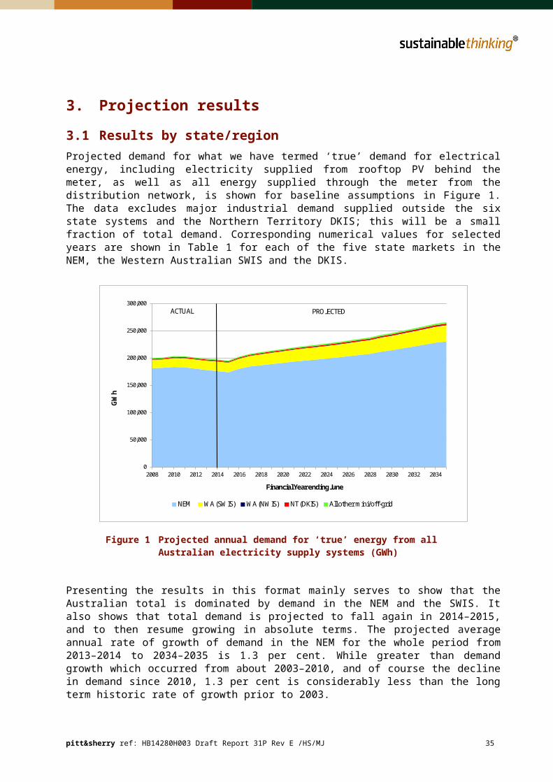
3.5 Annual peak demandThe relationship between annual energy and peak demand has been the subject of considerable public debate and controversy in recent years, which is unsurprising, given the magnitude of the changes in the relationship over recent years. In Victoria, Queensland and South Australia, annual electricity demand has clearly become more peaky in the last few years. The two main factors driving this change are penetration, i.e. ownership and capacity, of residential air-conditioning and the capacity of rooftop PV. The latter is probably the more important factor in Queensland and South Australia, which have significantly higher PV capacity (relative to total demand) than other states, while continuing growth in air-conditioning may be more important in Victoria.

As already noted, the equations we have developed relate peak demand to ‘true’ energy demand, including PV. It follows that the output numbers will include the contribution of PV to energy, as an input, and therefore also to peak, as the output. Consequently, to calculate peak load on the centralised system, it will be necessary to subtract an estimate of the PV contribution at time of peak in each state from the equation output value. This is a complex problem involving relationships which are continuing to evolve, and is outside the scope of this study. These projections also make no allowance for demand side participation at times of critical peak demand, which seems likely to be pursued more vigorously over the next few years by many network businesses, and by doing so will reduce demand on the network at peak times.

Projections of P50 annual peak demand for ‘true’ energy are shown in Figure 10 for New South Wales, Victoria and Queensland, and in Figure 11 for South Australia, Tasmania and Western Australia (SWIS). As can be deduced from the information in Section 2.8, states differ in how peak demand is affected by high temperatures and this shows up in the data presented in the two figures. In broad terms, however, rates of growth of P50 peak annual demand are affected by rates of growth in annual demand for electrical energy, which is why peak demand is projected to grow faster in Victoria and Western Australia than in other states.

The near-term fall in peak demand in Victoria is a consequence of the reduction in demand from the previously mentioned industrial closures, particularly the Point Henry smelter. It should be noted that this analysis assumes that at times of past critical peaks there was no demand side participation from these loads. This may not be correct, but we have no information as to whether or not it was the case. The projection may therefore under-estimate peak demand in Victoria. The near-term increase in Queensland, is a consequence of the demand increase from gas field compression, as previously discussed. Again, the implied assumption is that there will be no demand side participation by these loads at times of critical peaks, which may not be the case. It is also possible that in future years a larger and more active market for demand side participation at times of critical peaks may emerge, and many other circumstances may change, meaning that past behaviour by large consumers is not necessarily a reliable guide to future behaviour. These projections are therefore subject to unavoidable uncertainties, and these uncertainties may be somewhat larger for Victoria and Queensland than for the other states.

Figures 12 and 13 compare the results developed in this study by the corresponding projections of annual peak demand prepared by AEMO and IMO for New South Wales, Victoria, Queensland and Western Australia. The absolute levels are not directly comparable, because the AEMO and IMO projections are for native demand, and thus include transmission and distribution losses, but do not include PV. Our modelling also takes no explicit account of possible changes demand side participation, i.e. voluntary load shedding at times of critical peak demand. Nevertheless, in broad terms it is useful to compare the trends or annual changes of the respective projections.


Figure 10 Projected P50 annual peak demand for ‘true’ energy for New South Wales,Victoria and Queensland (MW)

Figure 11 Projected P50 annual peak demand for ‘true’ energy forSouth Australia, Western Australia and Tasmania (MW)


0

1,000

2,000

3,000

4,000

5,000

6,000

7,000

8,000

2006 2008 2010 2012 2014 2016 2018 2020 2022 2024 2026 2028 2030 2032 2034

MW

Financial Year ending JuneSA WA (SWIS) Tasmania

ACTUAL PROJECTED

0

2,000

4,000

6,000

8,000

10,000

12,000

14,000

16,000

2006 2008 2010 2012 2014 2016 2018 2020 2022 2024 2026 2028 2030 2032 2034

MW

Financial Year ending JuneNSW + ACT Victoria Queensland

ACTUAL PROJECTED

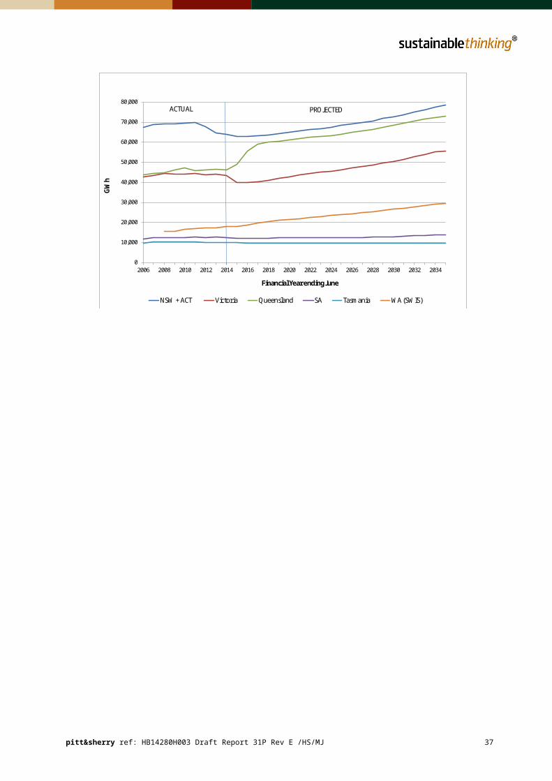
Figure 12 Projected P50 annual peak demand for ‘true’ energy compared with AEMOnative energy peak projections for New South Wales and Victoria (MW)

Figure 13 Projected P50 annual peak demand for ‘true’ energy compared with AEMO and IMO native energy peak projections for Queensland and Western Australia (SWIS) (MW)


0

2,000

4,000

6,000

8,000

10,000

12,000

14,000

16,000

2006 2008 2010 2012 2014 2016 2018 2020 2022 2024 2026 2028 2030 2032 2034

MW


NSW + ACT AEMO NSW Victoria AEMO Vic

ACTUAL PROJECTED

0

2,000

4,000

6,000

8,000

10,000

12,000

14,000

16,000

2006 2008 2010 2012 2014 2016 2018 2020 2022 2024 2026 2028 2030 2032 2034

MW

Financial Year ending JuneQueensland WA (SWIS) AEMO Qld IMO SWIS

ACTUAL PROJECTED

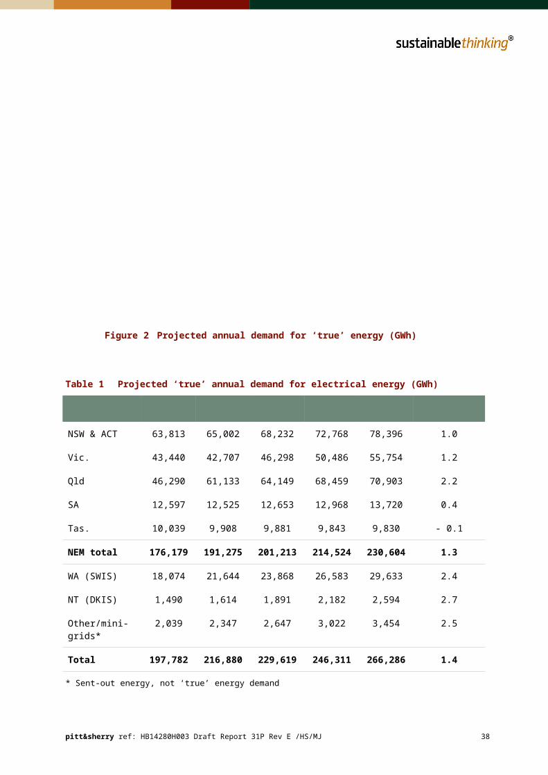
In every case, the relationship between our projections for peak demand and the corresponding AEMO and IMO projections closely resembles the corresponding relationships for projections of annual energy demand. We expect somewhat faster growth in energy demand and our results also show faster growth in annual peak demand. For Victoria, as shown in Table 3, AEMO projects particularly slow growth in energy demand, such that over the projections period it never exceeds the level in 2012–2013, prior to the closure of the Point Henry aluminium smelter. P50 annual peak demand accordingly remains almost constant, notwithstanding expected gradually increasing annual maximum temperatures. Our results, by contrast, are based on quite strong growth in energy demand, driven by the general business sector, for which we found a value of 0.95 for elasticity of demand with respect to GSP over recent years. As a result, and combined with the relatively high expected growth in Victorian GSP, we project that demand from this sector grows at an average rate of 1.9 per cent, which is higher than any other NEM state. In turn, we project total annual energy demand in Queensland to grow faster than in New South Wales, South Australia or Victoria. This faster energy demand growth, coupled with the effect of gradually increasing maximum temperatures on peak demand, explains the projected strong growth in peak demand.


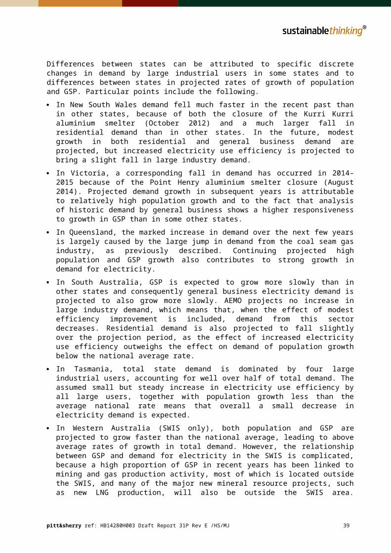
Appendix A

References

ABS 2014, Household energy consumption survey, Australia: summary of results, 2012. Cat. No. 4670.0, http://www.abs.gov.au/AUSSTATS/[email protected]/ProductsbyCatalogue/66AC0659BF300142CA257BEF0013D900?OpenDocument

ACIL Allen Consulting 2013, Electricity sector emissions – modelling of the Australian electricity generation sector, report to the Department of Innovation, Industry, Climate Change, Science, Research and Tertiary Education, September 2013, http://www.environment.gov.au/system/files/resources/65462f51-a20a-4f35-bdd0-d88d6ee5ac4e/files/electricty-sector-emissions.pdf

AEMO 2013, Forecasting methodology information paper, http://www.aemo.com.au/Electricity/Planning/Forecasting/National-Electricity-Forecasting-Report-2013/NEFR-Supplementary-Information-2013

AEMO 2014, 2014 national electricity forecasting report, http://www.aemo.com.au/Electricity/Planning/Forecasting/National-Electricity-Forecasting-Report

AER 2014, Network information – RIN responses, http://www.aer.gov.au/node/483

BREE 2013, Beyond the NEM and the SWIS 2011–12 regional and remote electricity in Australia, http://www.bree.gov.au/publications/beyond-nem-and-swis-2011%E2%80%9312-regional-and-remote-electricity-australia

BREE 2014a, Australian energy statistics update, http://www.bree.gov.au/publications/australian-energy-statistics

BREE 2014b, Resources and energy major projects.

Che, N and Pham, P 2012, Economic analysis of end-use energy intensity in Australia, BREE, Canberra, May 2012.

CSIRO 2007, Climate change in Australia: technical report.

ESAA various, Electricity gas Australia (annual).

George Wilkenfeld & Associates 2014, Impacts of the E3 program.

Graus, W, Blomen, E, Klessmann, C, Capone, C and Stricker, E 2009, Global technical potentials for energy efficiency improvement, presented at IAEE European Conference, September 2009.

IMO 2014, 2014 SWIS electricity demand outlook, http://www.imowa.com.au/home/electricity/reserve-capacity/electricity-statement-of-opportunities

Jacobs SKM 2014, Projections of gas and electricity used in LNG: public version, report prepared for AEMO.

Koomey, J, Rosenfeld, AH and Gadgil, A 1990, ‘Conservation screening curves to compare efficiency investments to power plants: applications to commercial sector conservation programs’, Proceedings 1990 ACEEE Summer Study on Energy Efficiency in Buildings.

Powerlink 2014, Transmission annual planning report 2014, http://www.powerlink.com.au/About_Powerlink/Publications/Transmission_Annual_Planning_Reports/Transmission_Annual_Planning_Report_2014.aspx

Productivity Commission 2013, Electricity Network Regulatory Frameworks, Volume 1. http://www.pc.gov.au/inquiries/completed/electricity/report

Saddler, H 2013, Power down: why is electricity consumption decreasing?, The Australia Institute. http://www.tai.org.au/content/power-down

pitt&sherry ref: document.docx/AUTHOR/word processor 42

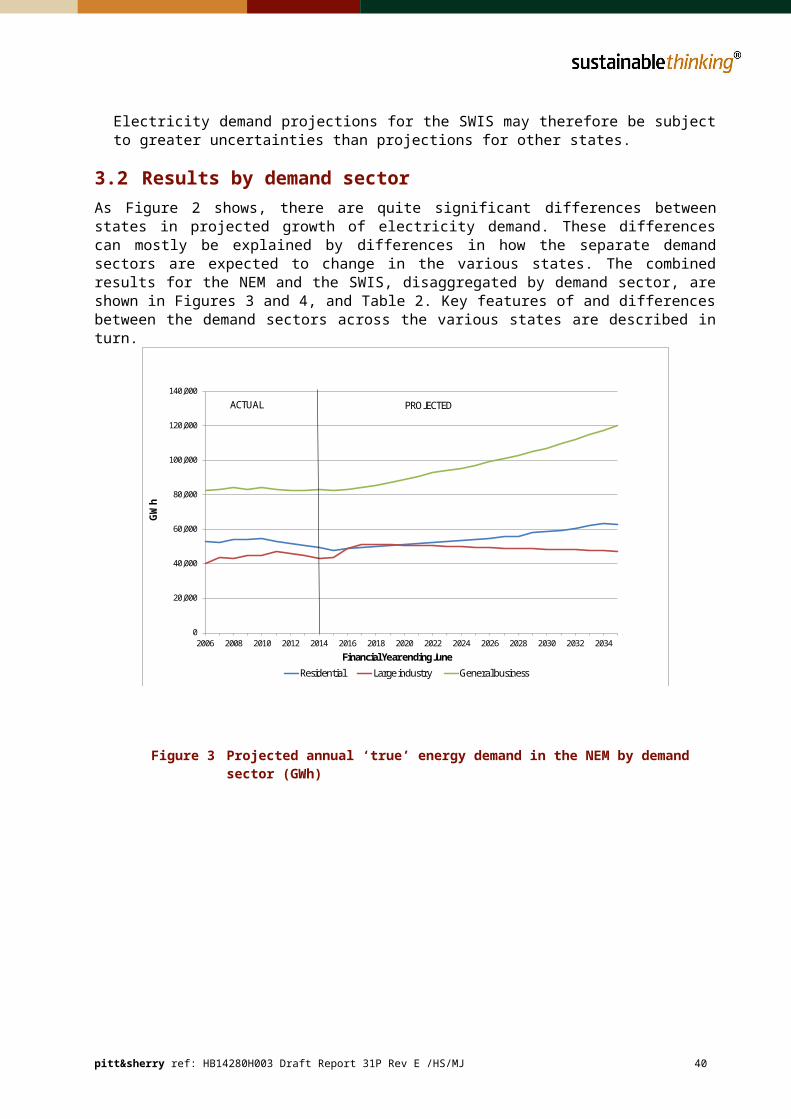
Treasury 2011, Strong growth, low pollution: modelling a carbon price: update. http://carbonpricemodelling.treasury.gov.au/content/default.asp


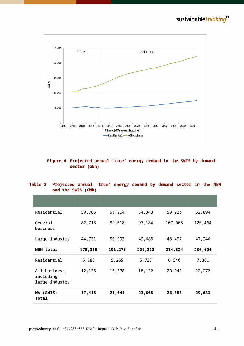
Appendix B

Abbreviations

ABS Australian Bureau of Statistics

AEMC Australian Energy Market Commission

AEMO Australian Energy Market Operator

AER Australian Energy Regulator

ANZSIC Australian and New ZealandStandard Industrial Classification

BCA Building Code of Australia

BREE Bureau of Resource and Energy Economics

CLF conservation load factor

DKIS Darwin–Katherine Interconnected System

E3 Equipment and Energy Efficiency program

ESAA Energy Supply Association of Australia

GJ gigajoule

GSP Gross State Product

GWh gigawatt-hour

IMO Independent Market Operator

kWh kilowatt-hour

LNG liquefied natural gas

MEPS Minimum Energy Performance Standards

MW megawatt

NABERS National Australian Built EnvironmentRating System

NEM National Electricity Market

NGERS National Greenhouseand Energy Reporting Scheme

NWIS North West Interconnected System

PV photovoltaic

SNSG small non-scheduled generator

SRES Small Renewable Energy Scheme

SWIS South West Interconnected System

TWh terawatt-hour

VEET Victorian Energy Efficiency Target


Appendix C

Glossary

behind-the-meter consumption The quantity of electricity produced (typically by rooftop PV) and consumed at a customer’s premises without ever passing through an electricity meter connected to the external distribution network.

coefficient of performance A term applied to air-conditioning systems, it is the ratio of the thermal energy output, i.e. the thermal energy removed from the conditioned space, to the electrical energy used to power the system. When reverse-cycle systems are used in heating mode, it is sometimes called the energy efficiency ratio.

electricity services In general, the term used to describe the useful services, such as light, motion and heat, provided by the use of electricity. For the specific purpose of this report the term is defined to mean the sum of electricity used by consumers and the additional quantity of electricity that would have been used had the electricity use efficiency of appliances, equipment and buildings remained at the average levels prevailing prior to the initial year used to calibrate the demand models, which is 2006.

native demand Operational demand plus electricity supplied by small generators other than rooftop PV.

operational demand The quantity of electricity supplied to an electricity supply

(identical with sent-out energy) system (the grid) by major generators (those dispatched by the system operator). It includes transmission and distribution losses.

small non-scheduled generators (SNSGs) Generators, other than rooftop PV, which are embedded within distribution networks; examples include cogeneration plants in commercial buildings, landfill gas generators and min-hydro plants.

‘true’ electricity demand The sum of electricity supplied to a consumer through the meter and electricity produced on site and consumed behind the meter.


Appendix D

Regulatory energy efficiency measures included in the models

Minimum Energy Performance StandardsData sources: George Wilkenfeld & Associates (2014); data provided by the Industry Department

Building Code of Australia Energy Efficiency ProvisionsData source: pitt&sherry analysis for previous studies for the Industry Department

Water Efficiency Labelling Standards as they affect demand for water heatingData source: George Wilkenfeld & Associates (2014)

The former Renewable Energy Target scheme (now the Small Renewable Energy Scheme), to the extent it accelerated the uptake of solar and heat pump water heaters above the rate prevailing prior to 2001Data source: pitt&sherry analysis of Clean Energy Regulator data

Mandatory disclosure of commercial building energy efficiencyData source: pitt&sherry analysis for previous studies for the Industry Department

Energy Efficiency in Government OperationsData source: pitt&sherry analysis for previous studies for the Industry Department

NABERS Data source: pitt&sherry analysis for previous studies for the Industry Department

New South Wales Energy Savings Scheme, Victorian Energy Efficiency Target, South Australian Residential Energy Efficiency Scheme, ACT Energy Efficiency Improvement Scheme Data source: Independent Pricing & Regulatory Tribunal (2012) Compliance and operation of the New South Wales Energy Savings Scheme during 2013

Note that these schemes award certificates based on the deemed lifetime energy (or emissions) saving from the efficiency measures undertaken. Energy savings from actions undertaken in past years were allocated to future years on the basis of the year each action was undertaken and the deemed life of the particular action concerned. Only past actions were included, as there is no way of knowing how much or what mix of allowed activities may be undertaken in future years. The Victorian, South Australian and Australian Capital Territory schemes were not included because either the majority of actions undertaken have a very short life, or were not unambiguously additional to other energy savings, e.g. MEPS, or because the estimated electricity savings, when spread over the deemed life, resulted in very small annual energy savings.


E: [email protected] W: www.pittsh.com.au

incorporated asPitt & Sherry (Operations) Pty LtdABN 67 140 184 309

BrisbaneLevel 2276 Edward StreetBrisbane QLD 4000T: (07) 3221 0080F: (07) 3221 0083

CanberraLGF, Ethos House28-36 Ainslie PlaceCanberra City ACT 2601PO Box 122Civic SquareCanberra ACT 2608T: (02) 6274 0100

DevonportLevel 135 Oldaker StreetPO Box 836Devonport TAS 7310T: (03) 6424 1641F: (03) 6424 9215

MelbourneLevel 1, HWT Tower40 City RoadSouthbank VIC 3006PO Box 259South Melbourne VIC 3205T: (03) 9682 5290F: (03) 9682 5292

Hobart199 Macquarie StreetGPO Box 94Hobart TAS 7001T: (03) 6210 1400F: (03) 6223 1299

LauncestonLevel 4113 Cimitiere StreetPO Box 1409Launceston TAS 7250T: (03) 6323 1900F: (03) 6334 4651

Contact

Hugh Saddler02 6274 [email protected]

Phil Harrington03 6210 [email protected]

Documents

… · Web view4. pitt&sherry ref: HB14280H003 Draft Report 31P Rev E /HS/MJ39. Pitt & Sherry ref: Outgoing Doc No/filename/filesection/ author/wordprocessor/Rev00. pitt& sherry