Young People’s Burden: Requirement of Negative CO2 Emissions

James Hansen,1 Makiko Sato,1 Pushker Kharecha,1 Karina von Schuckmann,2 David J Beerling,3 Junji Cao,4 Shaun Marcott,5 Valerie Masson-Delmotte,6 Michael J Prather,7 Eelco J Rohling,8,9 Jeremy Shakun,10 Pete Smith11

1Climate Science, Awareness and Solutions, Columbia University Earth Institute, New York, NY 10115 2Mercator Ocean, 10 Rue Hermes, 31520 Ramonville St Agne, France 3Leverhulme Centre for Climate Change Mitigation, University of Sheffield, Sheffield S10 2TN, UK 4Key Lab of Aerosol Chemistry and Physics, SKLLQG, Institute of Earth Environment, Xi’an 710061, China 5Department of Geoscience, 1215 W. Dayton St., Weeks Hall, University of Wisconsin-Madison, Madison, WI 53706 6Institut PierreSimon Laplace, Laboratoire des Sciences du Climat et de l’Environnement (CEA-CNRS-UVSQ) Université Paris Saclay, Gif-sur-Yvette, France 7Earth System Science Department, University of California at Irvine, CA 8Research School of Earth Sciences, The Australian National University, Canberra, 2601, Australia 9Ocean and Earth Science, University of Southampton, National Oceanography Centre, Southampton, SO14 3ZH, UK 10Department of Earth and Environmental Sciences, Boston College, Chestnut Hill, MA 02467 11Institute of Biological and Environmental Sciences, University of Aberdeen, 23 St Machar Drive, AB24 3UU, UK

E-mail: jeh1@columbia.edu

Keywords: climate change, carbon budget, intergenerational justice

AbstractThe rapid rise of global temperature that began about 1975 continues at a mean rate of about 0.18°C/decade, with the current annual temperature exceeding +1.25°C relative to 1880-1920. Global temperature has just reached a level similar to the mean level in the prior interglacial (Eemian) period, when sea level was several meters higher than today, and, if it long remains at this level, slow amplifying feedbacks will lead to greater climate change and consequences. The growth rate of climate forcing due to human-caused greenhouse gases (GHGs) increased over 20% in the past decade mainly due to resurging growth of atmospheric CH4, thus making it increasingly difficult to achieve targets such as limiting global warming to 1.5°C or reducing atmospheric CO2 below 350 ppm. Such targets now require “negative emissions”, i.e., extraction of CO2 from the atmosphere. If rapid phasedown of fossil fuel emissions begins soon, most of the necessary CO2 extraction can take place via improved agricultural and forestry practices, including reforestation and steps to improve soil fertility and increase its carbon content. In this case, the magnitude and duration of global temperature excursion above the natural range of the current interglacial (Holocene) could be limited and irreversible climate impacts could be minimized. In contrast, continued high fossil fuel emissions by the current generation would place a burden on young people to undertake massive technological CO2 extraction, if they are to limit climate change. Proposed methods of extraction such as bioenergy with carbon capture and storage (BECCS) or air capture of CO2 imply minimal estimated costs of 104-570 trillion dollars this century, with large risks and uncertain feasibility. Continued high fossil fuel emissions unarguably sentences young people to either a massive, possibly implausible cleanup or growing deleterious climate impacts or both, scenarios that should provide both incentive and obligation for governments to alter energy policies without further delay.

1

5

10

15

20

25

30

35

40

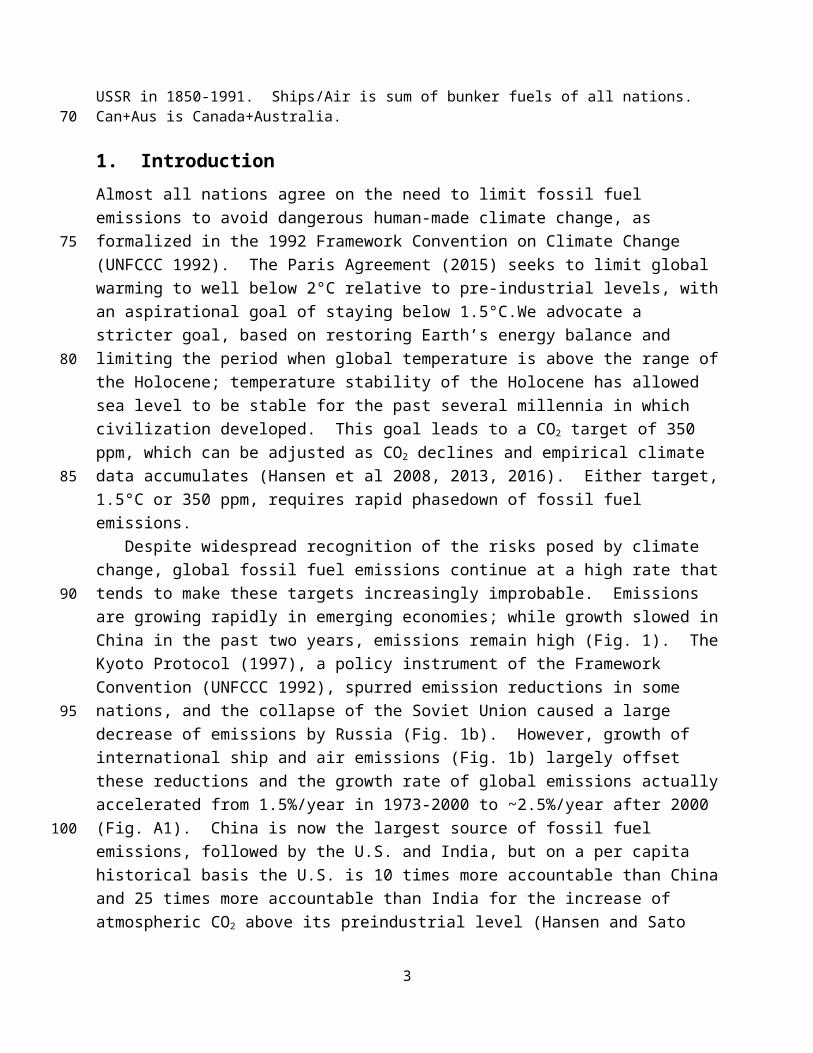
Fig. 1. Fossil fuel (and cement manufacture) CO2 emissions based on Boden et al (2016) with BP data used to infer 2014-2015 estimates. Europe/Eurasia is Turkey plus Boden et al categories Western Europe and Centrally Planned Europe. Asia Pacific is sum of Centrally Planned Asia, Far East and Oceania. Middle East is Boden et al Middle East less Turkey. Russia is Russian Federation since 1992 and 0.6 of USSR in 1850-1991. Ships/Air is sum of bunker fuels of all nations. Can+Aus is Canada+Australia.

1. IntroductionAlmost all nations agree on the need to limit fossil fuel emissions to avoid dangerous human-made climate change, as formalized in the 1992 Framework Convention on Climate Change (UNFCCC 1992). The Paris Agreement (2015) seeks to limit global warming to well below 2°C relative to pre-industrial levels, with an aspirational goal of staying below 1.5°C.We advocate a stricter goal, based on restoring Earth’s energy balance and limiting the period when global temperature is above the range of the Holocene; temperature stability of the Holocene has allowed sea level to be stable for the past several millennia in which civilization developed. This goal leads to a CO2 target of 350 ppm, which can be adjusted as CO2 declines and empirical climate data accumulates (Hansen et al 2008, 2013, 2016). Either target, 1.5°C or 350 ppm, requires rapid phasedown of fossil fuel emissions.

Despite widespread recognition of the risks posed by climate change, global fossil fuel emissions continue at a high rate that tends to make these targets increasingly improbable. Emissions are growing rapidly in emerging economies; while growth slowed in China in the past two years, emissions remain high (Fig. 1). The Kyoto Protocol (1997), a policy instrument of the Framework Convention (UNFCCC 1992), spurred emission reductions in some nations, and the collapse of the Soviet Union caused a large decrease of emissions by Russia (Fig. 1b). However, growth of international ship and air emissions (Fig. 1b) largely offset these reductions and the growth rate of global emissions actually accelerated from 1.5%/year in 1973-2000 to ~2.5%/year after 2000 (Fig. A1). China is now the largest source of fossil fuel emissions, followed by the U.S. and India, but on a per capita historical basis the U.S. is 10 times more accountable than China and 25 times more accountable than India for the increase of atmospheric CO2 above its preindustrial level (Hansen and Sato 2016). Tabular data for Figs. 1 and A1 are available on the web page www.columbia.edu/~mhs119/Burden.

In response to this situation, a lawsuit [Juliana et al vs United States 2016, hereafter J et al vs US 2016] was filed against the United States asking the U.S. District Court, District of Oregon, to require the U.S. government to produce a plan to rapidly reduce emissions. The suit requests that the plan reduce emissions at the 6%/year rate that Hansen et al (2013) estimated as the requirement for lowering atmospheric CO2 to a level of 350 ppm. At a hearing in Eugene Oregon on 9 March 2016 the United States and three interveners (American Petroleum Institute,

2

45

50

55

60

65

70

75

80

National Association of Manufacturers, and the American Fuels and Petrochemical Association) asked the Court to dismiss the case, in part based on the argument that the requested rate of fossil fuel emissions reduction was implausible. Magistrate Judge Coffin stated that he was “troubled” by the severity of the requested emissions reduction rate, but he also noted that some of the alleged climate change consequences, if accurate, could be considered “beyond the pale”, and he rejected the motion to dismiss the case. Judge Coffin’s ruling must be certified by a second judge, after which the case can proceed to trial. It is anticipated that the plausibility of achieving the emission reductions needed to stabilize climate will be a central issue at the trial.

Urgency of initiating emissions reductions is well recognized (IPCC 2013, 2014; Huntingford et al 2012; Friedlingstein et al 2014; Rogelj et al 2016a) and was stressed in the paper that the lawsuit J et al vs US (2016) uses to prescribe an emissions reduction scenario (Hansen et al 2013). The climate research community also realizes that the goal to keep global warming less than 1.5°C probably requires negative net CO2 emissions later this century if high global emissions continue in the near-term (Fuss et al 2014; Anderson 2015; Rogelj et al 2016b; Sanderson et al 2016). The Intergovernmental Panel on Climate Change (IPCC) reports (IPCC 2013, 2014) do not address environmental and ecological feasibility and impacts of large-scale CO2 removal, but recent studies (Smith et al 2016; Williamson 2016) are taking up this crucial issue and raising the question of whether large-scale negative emissions are even feasible.

Our aim is to contribute to understanding of the threshold-required rate of CO2 emissions reduction via an approach that is transparent to non-scientists. We consider the potential for reductions of non-CO2 GHGs to minimize the human-made climate forcing, the potential for improved agricultural practices to store more soil carbon, and the potential drawdown of atmospheric CO2 from reforestation and afforestation. Quantitative examination reveals the merits of these actions to ameliorate demands on fossil fuel CO2 emission phasedown, but also the limitations, thus clarifying the urgency of government actions to rapidly advance the transition to carbon-free energies to meet the climate stabilization targets they have set.

We first describe the status of global temperature change and then summarize the principal climate forcings that drive long term climate change. We show that observed global warming is consistent with knowledge of changing climate forcings, Earth’s measured energy imbalance, and the canonical estimate of climate sensitivity, i.e., about 3°C1 global warming for doubled atmospheric CO2. We illustrate updates of GHG observations and calculate a notable acceleration during the past decade of the growth rate of GHG climate forcing. For future fossil fuel emissions we consider both the IPCC Representative Concentration Pathways (RCP) scenarios, and simple emission growth rates that are helpful for determination of the plausibility of required emission changes. We use a precisely defined Green’s function calculation of global temperature with canonical climate sensitivity for each emissions scenario, thus allowing us to determine the amount of CO2 that must be extracted from the air – effectively the climate debt – to achieve the targets of returning atmospheric CO2 to less than 350 ppm or limiting global warming to less than 1.5°C above preindustrial levels. We discuss alternative extraction technologies and their estimated costs, and finally we consider the potential alleviation of CO2 extraction requirements that might be obtained via special efforts to reduce non-CO2 GHGs.

1 IPCC (2013) finds that 2×CO2 equilibrium sensitivity is likely in the range 3 ± 1.5°C, as was estimated by Charney et al. (1979). Median sensitivity in recent model inter-comparisons is 3.2°C (Andrews et al 2012; Vial et al 2013).

3

85

90

95

100

105

110

115

120

Fig. 2. Global surface temperature relative to 1880-1920 based on GISTEMP analysis (Appendix A). (a) Annual and 5-year means since 1880, (b) 12- and 132-month running means since 1970. Black squares in (b) are calendar year (Jan-Dec) year means used to construct (a). (b) uses data through August 2016.

2. Global Temperature ChangeThe United Nations 1992 Framework Convention on Climate Change (UNFCCC 1992) stated its objective as ‘…stabilization of GHG concentrations in the atmosphere at a level that would prevent dangerous anthropogenic interference with the climate system’. The 15th Conference of the Parties (Copenhagen Accord 2009) concluded that this objective required a goal to ‘…reduce global emissions so as to hold the increase of global temperature below 2°C…’ and that the 2015 Conference of the Parties should consider the possibility of strengthening the temperature limit to below 1.5°C. Indeed, the Paris Agreement (2015) modified the objective ‘to holding the increase of global average temperature to well below 2°C above pre-industrial levels and to pursue efforts to limit the temperature increase to 1.5°C above preindustrial levels…’.

Defining a target for limiting human interference with natural climate requires quantitative assessment of ongoing and paleo temperature changes, with the latter especially helpful for characterizing long-term ice sheet and sea level response versus temperature. We examine the modern period with near-global instrumental temperature data in the context of the current and previous (Holocene and Eemian) interglacial periods for which less precise proxy-based temperatures have recently emerged. The Holocene, now over 11,700 years in duration, has had relatively stable climate. The Eemian, lasting from about 130,000 to 115,000 years ago, was moderately warmer than the Holocene.

2.1. Modern Temperature The several analyses of temperature change since 1880 are in close agreement (Hartmann et al 2013). Thus we can use the current GISTEMP analysis (see Supporting Information), which is updated monthly and available (http://www.columbia.edu/~mhs119/Temperature/).

The popular measure of global temperature is the annual-mean global-mean value (Fig. 2a), which is publicized at the end of each year. However, as discussed by Hansen et al. (2010), the 12-month running mean global temperature is more informative and removes monthly “noise” from the record just as well as the calendar year average. For example, the 12-month running

4

125

130

135

140

145

150

mean for the past 35 years (Fig. 2b) defines clearly the super-El Niños of 1997-98 and 2015-16 and the 3-year cooling after the Mount Pinatubo volcanic eruption in the early 1990s.

Global temperature in each month for the past year has been at or near a record for the month. Perhaps helped by a popular “spiral” temperature visualization (Hope 2016), this has tended to create a popular impression that global temperature may be spiraling out of control. This series of monthly records is likely to terminate soon and the 12-month running mean is expected to decline as it has after prior El Niños. However, the year-to-date temperature is so far above the prior record already that even the steepest post-El Niño decline cannot prevent a 2016 annual record temperature.

One effect of the recent warming is to remove unequivocally the illusion of a global warming hiatus after the 1997-98 El Niño. Several studies, including Trenberth and Fasullo (2013), England et al. (2014), Dai et al. (2015) and Rajaratnam et al (2015), showed that temporary plateaus are consistent with expected long-term warming due to increasing atmospheric GHGs. Other analyses of this specific plateau help illuminate the roles of unforced climate variability and natural and human-caused climate forcings in observed climate change, with the Interdecadal Pacific Oscillation (a recurring pattern of ocean-atmosphere climate variability) playing a major role in the warming slowdown (Kosaka and Xie, 2013; Meehl et al, 2014; Fyfe et al, 2016).

Global temperature defined by the linear fit over recent decades has now reached +1.06°C relative to the 1880-1920 average (Fig. 2), the 12-month running mean temperature through August 2016 is 1.30°C, and the 2016 temperature likely will be near +1.25°C. The present global warming rate, based on a linear fit through the past 45 years (dashed line in Fig. 2b) is +0.18°C per decade. At this rate, the trend line of global temperature, which is a relevant measure of mean temperature, will reach +1.5°C in about 2040 and +2°C in the late 2060s. However, the warming rate can accelerate or decelerate, depending on policies that affect GHG emissions, developing climate feedbacks, and other factors discussed below.

2.2. Temperature during current and prior interglacial periods Holocene temperature has been reconstructed at centennial-scale resolution from 73 globally distributed proxy temperature records by Marcott et al (2013). This record shows a decline of 0.6°C from early Holocene maximum temperature to a “Little Ice Age” minimum in the early 1800s [that minimum being better defined by higher resolution data of Abram et al (2016)].

Concatenation of the modern and Holocene temperature records (Fig. 3) assumes, based on Abram et al (2016), that the 1880-1920 mean temperature is 0.1°C warmer than the Little Ice Age minimum. The early Holocene maximum in the Marcott et al (2013) data is thus at +0.5°C relative to the 1880-1920 mean of the modern data. However, model simulations suggest that the reconstructed early Holocene maximum may be ezaggerated due to limitations of the proxy data, especially potential seasonality bias, as discussed by Marcott et al (2013) and Liu et al (2014).

Even though we cannot be certain that the current year is warmer than any single year earlier in the Holocene due to centennial smoothing of the Holocene stack and original resolution of the underlying proxy records (Marcott et al 2013), we conclude that the ongoing global warming trend (1.06°C over 115 years, Fig 2b) is already well above prior centennially smoothed Holocene temperature. Further, we suggest that these smoothed temperatures are relevant to

5

155

160

165

170

175

180

185

190

195

Fig. 3. Estimated average global temperature for the last interglacial (Eemian) period (McKay et al 2011; Clark and Huybers 2009; Turney and Jones 2010), the centennially-smoothed Holocene (Marcott et al 2013) temperature as a function of time, and the 11-year mean of modern data (Fig. 2). Vertical downward arrows indicate likely overestimates (see text).

important climatic features that change on long time scales, such as ocean warming (von Schuckmann et al 2016), ice sheet stability (DeConto and Pollard 2016), shifting climatic zones (Seidel et al 2008), and the frequency of climate extremes (Hansen and Sato 2016). The formal 2σ (95% confidence) uncertainty in the Marcott et al (2013) Holocene temperature curve is only ~0.25°C. Although total uncertainty is larger, because of issues such as discussed by Liu et al (2014), those uncertainties tend to push the early Holocene temperatures lower, increasing the gap between today’s temperature and early Holocene temperature (Marcott and Shakun 2015).

We also conclude that the modern trend line of global temperature crossed the early Holocene (smoothed) temperature maximum (+0.5°C) already in about 1985. This conclusion receives support from the accelerating rate of sea level rise, which approached a rate of 3 mm/year at about that date (Fig. 29 of Hansen et al 2016 shows a relevant concatenation of measurements). Such a high rate of sea level rise, which equates to 3 meters per millennium, far exceeds rates of Holocene sea level rise except in the earliest Holocene when melt was still coming from the final decay of mid-latitude ice sheets (Dutton et al 2015).

The Framework Convention (UNFCCC 1992) and Paris Agreement (2015) define goals relevant to ‘preindustrial’ temperature, but do not define that period. We use 1880-1920, the earliest time with good global coverage of instrumental data, as the zero-point for temperature anomalies. Alternatively, one might argue for defining preindustrial as the Little Ice Age minimum temperature, but the deep ocean did not have time to reach equilibrium with those brief conditions, and global mean Little Ice Age temperature was probably only ~0.1C cooler than the 1880-1920 mean (Abram et al 2016).

The important point is that the relevant mean global temperature has already risen out of the centennial Holocene range. Global warming is already having substantial adverse climate impacts (IPCC 2014), including extreme events (NAS 2016), and there is widespread agreement that 2°C warming would commit the world to multi-meter sea level rise (Levermann et al 2013; Clark et al 2016), and a case has been made that this could unfold within 50-150 years (Hansen et al 2016).

The prior interglacial period, the Eemian, was warmer than the Holocene and sea level reached heights 6-9 m (20-30 feet) higher than today (Dutton et al (2015). McKay et al (2011)

6

200

205

210

215

220

225

230

estimated peak Eemian annual global ocean SST as +0.7°C ± 0.6°C, while models, as described by Masson-Delmotte (2013), give more confidence to the lower part of that range. Global ocean SST response to climate forcings is typically 70-75% as large as the global mean (land + ocean) surface temperature response and that same proportion is found empirically in the warming of the past century (http://www.columbia.edu/~mhs119/Temperature/T_moreFigs/). Thus the McKay et al data are equivalent to a global Eemian temperature +1°C relative to the Holocene. Clark and Huybers (2009) and Turney and Jones (2010) estimated global temperature in the Eemian as 1.5-2°C warmer than the Holocene (Fig. 3), but Bakker and Renssen (2014) analyzed the likely error in Eemian temperature estimates caused by the assumption that maximum Eemian temperatures at all proxy temperature sites occurred simultaneously and also the effect of proxy biases towards summer conditions, concluding that these biases could exaggerate Eemian temperature by 1.1 ± 0.4°C. Thus, consistent with the discussion of Masson-Delmotte (2013), we conclude that mean Eemian temperature was probably about 1°C warmer than the Holocene. Given growing indications, discussed above, that the early Holocene was little warmer than the pre-industrial (1880-1920) period, we conclude that Eemian global temperature was not much more than +1°C relative to 1880-1920 global temperature.

These considerations add to the question of whether 2°C, or even 1.5°C, is an appropriate target to protect the well-being of young people and future generations, as modeling projections compared to these targets usually include only fast-feedback processes. Indeed, Hansen et al (2008) concluded “If humanity wishes to preserve a planet similar to that on which civilization developed and to which life on Earth is adapted, paleoclimate evidence and ongoing climate change suggest that CO2 will need to be reduced from its (then) current 385 ppm to at most 350 ppm, but likely less than that.” And further “If the present overshoot of the target CO2 is not brief, there is a possibility of seeding irreversible catastrophic effects.”

A danger of the 1.5°C and 2°C temperature targets is that they are far above the Holocene temperature range. If such temperature levels are allowed to long exist they will spur “slow” amplifying feedbacks (Hansen et al 2013; Rohling et al 2013; Masson-Delmotte et al 2013), which may have potential to run out of humanity’s control. The most threatening slow feedback likely is ice sheet melt and consequent sea level rise, but there are other risks in pushing the climate system far out of its Holocene range. Methane release from melting permafrost and methane hydrates is also a potentially important feedback, for example, although there are large gaps in our understanding of this feedback including its time-scale (O’Connor et al 2011).

Thus in this paper we examine the fossil fuel emission reductions required to restore atmospheric CO2 to 350 ppm or less, so as to keep global temperature close to the Holocene range, in addition to the canonical 1.5°C and 2°C targets. Quantitative investigation requires consideration of Earth’s energy imbalance, changing climate forcings, and climate sensitivity.

7

235

240

245

250

255

260

265

Fig. 4. Estimated effective climate forcings (update of Hansen et al 2005 through 2015). Forcings are based on actual changes of each gas, except CH4-induced changes of O3 and stratospheric H2O are included in the CH4 forcing. Oscillatory and intermittent natural forcings (solar irradiance and volcanoes) are excluded. CFCs include not only chlorofluorocarbons, but all Montreal Protocol Trace Gases (MPTGs) and Other Trace Gases (OTGs).

3. Global Climate Forcings and Earth’s Energy ImbalanceThe dominant human-caused drivers (forcings) of climate change are changes of atmospheric GHGs and aerosols. GHGs absorb Earth’s infrared (heat) radiation, thus serving as a “blanket” that warms Earth’s surface. Aerosols, fine particles in the air that cause visible air pollution, both reflect and absorb solar radiation, but reflection of solar energy to space is their dominant effect, so they cause a cooling that partly offsets GHG warming. Estimated forcings (Fig. 4), an update of Fig. 28b of Hansen et al (2005), are similar to those of Myhre et al (2013) in the most recent IPCC report (IPCC 2013).

Climate forcings in Fig. 4 are the planetary energy imbalance caused by preindustrial-to-present change of each atmospheric constituent. The CH4 forcing includes its indirect effects, as increasing atmospheric CH4 causes tropospheric ozone (O3) and stratospheric water vapor to increase (Myhre et al 2013). Uncertainties in the forcings, discussed by Myhre et al (2013), are typically 10-15% for GHGs. Uncertainty in the aerosol forcing, described by a probability distribution function (Boucher et al 2013), is of order 50%. Our estimate of aerosol + surface albedo forcing (−1.2 W/m2) differs from the −1.5 W/m2 of Hansen et al (2005), as discussed below, but both are within the range of the distribution function of Boucher et al (2013).

The positive net forcing (Fig. 4) causes Earth to be out of energy balance, with more energy coming in than going out, which drives slow global warming. Eventually Earth will become hot enough to radiate to space an amount of energy matching absorbed sunlight. However, because of the ocean’s great thermal inertia (heat capacity), full atmosphere-ocean response to the forcing requires a long time: atmosphere-ocean models suggest that even after 100 years only 60-75% of the surface warming for a given forcing has occurred, the remaining 25-40% still being “in the pipeline” (Hansen et al 2011; Collins et al 2013). Moreover, we will outline in the next section that global warming can activate “slow” feedbacks, such as changes of ice sheets or melting of methane hydrates, so the time for the system to reach a fully equilibrated state is even longer.

GHGs have been increasing for more than a century and Earth has partially warmed in response. Earth’s energy imbalance is the portion of the forcing that has not yet been responded to. This imbalance thus defines additional global warming that will occur without further change

8

270

275

280

285

290

295

300

Fig. 5. Ocean heat uptake in upper 2 km of ocean during 11 years 2005-2015 using analysis method of von Schuckmann and LeTraon (2011). Heat uptake in W/m2 (0.5 and 0.7) refer to global (ocean + land) area, i.e., it is the contribution of the upper ocean to the heat uptake averaged over the entire planet.

of forcings. Earth’s energy imbalance can be measured by monitoring ocean subsurface temperatures, because almost all excess energy coming into the planet goes into the ocean (von Schuckmann et al 2016). Most of the ocean’s heat content change occurs in the upper 2000 m (Levitus et al 2012), which has been well measured since 2005 when the distribution of diving Argo floats achieved good global coverage (von Schuckmann and Le Traon 2011).

Earth’s energy imbalance was about +0.6 W/m2 during 2005-2010 (Hansen et al 2011) as inferred from heat gain in the upper 2 km of ocean using the von Schuckmann and Le Traon (2011) analysis and adding the smaller heat gain by the deep ocean (Purkey and Johnson 2013), continents, atmosphere, and net melting of sea ice and land ice. Accounting for the declining solar irradiance during 2005-2010 (Fig. A3), Hansen et al (2011) inferred that the energy imbalance with the solar cycle effect removed was +0.75 ± 0.25 W/m2. Here we update the von Schuckmann and Le Traon analysis with data for 2005-2015 (Fig. 5) finding 0.7 W/m2 heat uptake in the upper 2000 m of the ocean. The 11-year period now available (2005-2015) should practically eliminate a solar cycle influence. The small heat gains noted above add of order 0.1 W/m2 to the global heat gain (Rhein et al 2013), so our current analysis is consistent with a planetary energy imbalance of +0.75 ± 0.25 W/m2. The value 0.75 W/m2 is near the middle of a range of estimates by several investigators (von Schuckmann et al 2016; Trenberth et al 2016).

4. Climate Sensitivity, a Consistency Check and Slow Feedbacks Climate sensitivity has been a fundamental issue since at least the 19th century when Tyndall (1861) and Arrhenius (1896) stimulated interest in the effect of a CO2 change on climate. Doubled atmospheric CO2, a forcing of about 4 W/m2, is now a standard forcing in studies of climate sensitivity. The Charney et al (1979) study concluded that equilibrium sensitivity, i.e., global warming after a time sufficient for the planet to restore energy balance with space, was 3°C ± 1.5°C for 2×CO2 or 0.75°C per W/m2 forcing. The central value found in a wide range of modern climate models (Flato et al 2013) and in empirical paleoclimate studies remains 3°C for 2×CO2, but with an uncertainty that is still of order 1°C (Rohling et al 2012a).

An important consistency check is obtained by comparing the estimated net climate forcing (2.5 W/m2, Fig. 4), Earth’s energy imbalance (~0.75 W/m2), observed global warming, and climate sensitivity. Observed warming since 1880-1920 is 1.06°C with the effect of El Niño/La

9

305

310

315

320

325

330

335

Niña oscillations removed (Fig. 2b). Global warming between 1700-1800 and 1880-1920 was ~0.1°C (Abram et al 2016; Marcott et al 2013), so 1750-2015 warming was ~1.16°C. Taking climate sensitivity as 0.75°C per W/m2 forcing, global warming of 1.16°C implies that 1.55 W/m2 of the total 2.5 W/m2 forcing has been “used up” to cause observed warming. Thus 0.95 W/m2 forcing should remain to be responded to, i.e., the expected planetary energy imbalance is 0.95 W/m2, reasonably consistent with the observed 0.75 ± 0.25 W/m2. If we instead use the aerosol + surface albedo forcing −1.5 W/m2 estimated by Hansen et al (2005), the net climate forcing is 2.2 W/m2 and the forcing not responded to is 0.65 W/m2, which is also within the observational error of Earth’s energy imbalance.

An important matter to bear in mind is that the sensitivity 3°C for 2×CO2 (0.75°C per W/m2) is the “fast-feedback” climate sensitivity, i.e., it does not include “slow” climate feedbacks that will occur if global temperature long remains above the Holocene level (Hansen et al 2008; Rohling et al 2012a). Slow feedbacks include large-scale shrinking of ice sheets as Earth warms and the enhanced release of GHGs as the ocean, soil, and continental shelves warm. These slow feedbacks are strongly amplifying, indeed, they are the reason that natural long-term climate oscillations are so large in response to even small long-term global-average forcings (Rohling et al 2012b; Masson-Delmotte et al 2013).

The fast-feedback climate sensitivity is the appropriate sensitivity to use in interpretation of recent climate change, because we use observed change of GHGs and because ice sheet change so far is small. However, the need to avoid the emergence of slow feedbacks motivates the criterion that energy balance should be restored at a global temperature close to and eventually within the Holocene range (Hansen et al. 2008, 2013).

Earth’s present energy imbalance is causing heat to accumulate in the ocean, where it contributes to melting of ice shelves (Rignot et al 2013). Rising temperatures also increase the risk of CO2 and CH4 release from drying soils, thawing permafrost (Schadel et al 2016; Schuur et al 2015) and warming continental shelves (Kvenvolden 1993, Judd et al 2002). Time scales for the slow feedbacks are not well established, but recent modeling and empirical evidence suggest that substantial ice sheet and sea level changes could occur within periods as short as several decades (Rohling et al 2013; Pollard et al 2015; Hansen et al 2016). If large planetary energy imbalance continues, there is a danger that the warming driving slow feedbacks will be so far advanced that consequences such as large sea level rise proceed out of humanity’s control.

Quantification of requirements for stabilizing climate depends on knowledge of ongoing changes of the two largest GHG forcings, CO2 and CH4. It is also necessary to understand how we are changing GHG emissions directly through industrial and agricultural activities (designated ‘anthropogenic emissions’ and included in the SRES and RCP scenarios) and indirectly through climate change (the slow feedbacks noted above, designated somewhat paradoxically ‘natural emissions’ changes, and not included in the SRES and RCP scenarios).

10

340

345

350

355

360

365

370

375

Fig. 6. (a) Global CO2 annual growth based on NOAA data (http://www.esrl.noaa.gov/gmd/ccgg/trends/). Dashed curve is for a single station (Mauna Loa). Red curve is monthly global mean relative to the same month of prior year; black curve is 12-month running mean of red curve. (b) CO2 growth rate is highly correlated with global temperature, the CO2 change lagging global temperature change by 8 months.

5. Observed CO2 and CH4 Growth RatesAnnual increase of atmospheric CO2, averaged over a few years, grew from less than 1 ppm/year 50 years ago to more than 2 ppm/year today (Fig. 6), with the global mean and Mauna Loa CO2 amounts now exceeding 400 ppm (Betts et al 2016). The large oscillations of the annual growth are correlated with global temperature and with the El Niño/La Niña cycle2. Correlations are calculated for the 12-month running means, which effectively remove the seasonal cycle and monthly noise. Maxima of the CO2 growth rate lag global temperature maxima by ~8 months (Fig. 6b) and lag Niño3.4 [latitudes 5N-5S, longitudes 120-170W] temperature by ~10 months. These lags imply that the current CO2 growth spike (Fig. 6 uses data through July 2016), associated with the 2015-16 El Niño, may not have reached its maximum yet, as Niño3.4 peaked in December 2015 and global temperature peaked in February 2016.

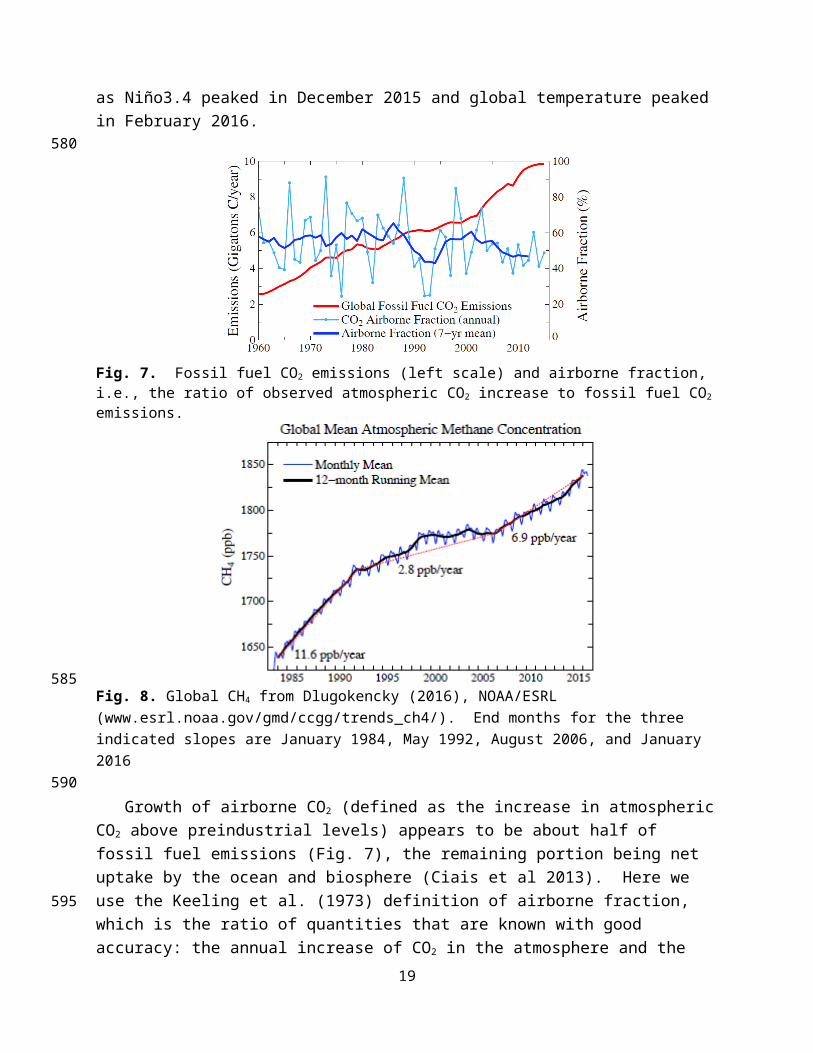
Fig. 7. Fossil fuel CO2 emissions (left scale) and airborne fraction, i.e., the ratio of observed atmospheric CO2 increase to fossil fuel CO2 emissions.

2 One mechanism for greater than normal atmospheric CO2 growth during El Niños is the impoverishment of nutrients in equatorial Pacific surface water and thus reduced biological productivity that result from reduced upwelling of deep water (Chavez et al., 1999). However, the El Niño/La Niña cycle seems to have an even greater impact on atmospheric CO2 via the terrestrial carbon cycle through effects on the water cycle, temperature, and fire, as discussed in a large body of literature (referenced, e.g., by Schwalm et al., 2011).

11

380

385

390

395

5

Fig. 8. Global CH4 from Dlugokencky (2016), NOAA/ESRL (www.esrl.noaa.gov/gmd/ccgg/trends_ch4/). End months for the three indicated slopes are January 1984, May 1992, August 2006, and January 2016

Growth of airborne CO2 (defined as the increase in atmospheric CO2 above preindustrial levels) appears to be about half of fossil fuel emissions (Fig. 7), the remaining portion being net uptake by the ocean and biosphere (Ciais et al 2013). Here we use the Keeling et al. (1973) definition of airborne fraction, which is the ratio of quantities that are known with good accuracy: the annual increase of CO2 in the atmosphere and the annual amount of CO2 injected into the atmosphere by fossil fuel burning. The data reveal that, even as fossil fuel emissions have increased by a factor of four over the past half century, the ocean and biosphere have continued to take up about half of the emissions (Fig. 7, right-hand scale). This seemingly simple relation between emissions and atmospheric CO2 growth is not predictive as it depends on the growth rate of emissions being maintained, and, indeed, it is not expected to continue in cases with major changes in the emission scenario, so we use a carbon cycle model in Section 7 to compute atmospheric CO2 as a function of emission scenario.

Atmospheric CH4 stopped growing between 1998 and 2006, indicating that its sources and sinks were nearly in balance, but growth resumed in the past decade (Fig. 8). Growth of CH4 exceeds 10 ppb/year in 2014 and 2015, almost as fast as in the 1980s). Turner et al. (2016) suggest that increased fossil fuel emissions in the U.S. may be a major cause of renewed global CH4 growth. However, CH4 isotope data imply that resumed growth was mainly from wetlands, especially in the tropics but with a contribution from high latitudes of the Northern Hemisphere (Bousquet et al 2011; Dlugokencky et al 2011). The CH4 changes over the past two decades are driven primarily by changes in emissions as observations of CH3CCl3 show very little change in the atmospheric sink for CH4 (Montzka et al. 2011; Holmes et al. 2013). Future changes in the sink, however, are expected to lead to increased atmospheric CH4 separate from emission changes, but these are difficult to project in the RCP scenarios (Voulgarakis et al. 2013).

The continued growth of atmospheric CO2 and the reaccelerating growth of CH4 raise important questions related to prospects of stabilizing climate. How consistent are scenarios for phasing down climate forcing with reality revealed by observational data? What changes to emissions are required to stabilize climate? We address these issues below.

12

400

405

410

415

420

425

Fig. 9. GHG climate forcing growth rate with historical data being 5-year running means, except data for 2014 and 2015 are 3- and 1-year means. (a) includes scenarios used in IPCC AR3 and AR4 reports, and (b) has AR5 scenarios. N2O, MPTGs and OTGs (Montreal Protocol Trace Gases and Other Trace Gases) data are from NOAA/ESRL Global Monitoring Division.

6. GHG Climate Forcing Growth Rates and Emission ScenariosInsight is obtained by comparing the growth rate of GHG climate forcing based on observed GHG amounts with past and present GHG scenarios. We examine forcings of IPCC SRES (2000) scenarios used in the AR3 and AR4 reports (Fig. 9a) and RCP scenarios (IPCC 2013) used in the AR5 report (Fig. 9b). We include the “alternative scenario” of Hansen et al (2000) in which CO2 and CH4 emissions decline such that global temperature stabilizes near the end of the century.3 We use the same radiation equations for observed GHG amounts and scenarios, so errors in the radiation calculations do not alter the comparison. Equations for GHG forcings are from Table 1 of Hansen and Sato (2004) with the CH4 forcing using an efficacy factor 1.4 to include effects of CH4 on tropospheric O3 and stratospheric H2O (Hansen et al 2005).

The growth of GHG climate forcing peaked at ~0.05 W/m2/year (5 W/m2/century) in 1978-1988, then falling to a level 10-25% below IPCC SRES (2000) scenarios during the first decade of the 21st century (Fig. 9a). The decline was due to (1) decline of the airborne fraction of CO2 emissions (Fig. 7), (2) slowdown of CH4 growth (Fig. 8), and (3) the Montreal Protocol, which initiated phase-out of gases that destroy stratospheric ozone.

The situation in 2000 seemed ripe for a pathway to climate stabilization more rapid than any of the IPCC scenarios. The slowing growth of forcings was partly good fortune, but also due to

3This scenario is discussed by Hansen and Sato (2004). CH4 emissions decline moderately, producing a small negative forcing. CO2 emissions (not captured and sequestered) are assumed to decline until in 2100 fossil fuel emissions just balance uptake of CO2 by the ocean and biosphere. CO2 emissions continue to decline after 2100.

13

430

435

440

445

450

10

Fig. 10. Fossil fuel emission scenarios. Scenarios in (a) have constant emissions in 2015-2020 and then simple specified rates of emission increase or decrease. IPCC (2013) RCP scenarios are shown in (b).

the prescience of the Montreal Protocol, whose design and implementation to reduce the ozone-depleting gases also allowed it to be used to slow or reverse growth of some other GHGs. The alternative scenario aimed to extend the downward trend in the growth rate of climate forcing by: (1) slowing the growth of CO2 emissions, as may occur with a substantial rising price on carbon emissions to accelerate development of carbon-free energies, (2) a global effort to reduce CH4 emissions, (3) continued use and tightening of the Montreal Protocol to constrain trace GHGs. The slowly decreasing forcing of this alternative scenario would have kept global warming well below 1.5°C, for climate sensitivity 0.75°C/W/m2 (Fig. A4).

However, in reality, in the absence of a universally rising carbon price and substantial support for energy research and development, global fossil fuel CO2 emissions accelerated, from 1.5%/year in 1973-2000 to ~2.5%/year after 2000 (Figs. 1 and S1). The growth rate of GHG forcing now exceeds the alternative scenario by ~70% (Fig. 9a). New scenarios must begin from current reality, and, as a consequence or recent growth, ambitious targets for limiting global warming now require much steeper emissions reductions.

The new IPCC (2013) RCP scenarios (Fig. 9b) initiate in 2011 and fan out into an array of potential futures driven by assumptions about energy demand, fossil fuel prices, and climate policy, chosen to be representative of an extensive literature on possible emissions trajectories (Moss et al 2010; van Vuuren et al 2011; Meinshausen et al 2011). Numbers on the RCP scenarios (8.5, 6.0, 4.5 and 2.6) refer to the GHG climate forcing (W/m2) in 2100.

As a complement to RCP scenarios, we define scenarios simply by percent annual emission decrease or increase. We consider rates −6%/year, −3%/year, constant emissions, and +2%/year; emissions stop increasing in the +2%/year case when they reach 25 Gt/year (Fig. 10a). Scenarios with decreasing emissions are preceded by constant emissions for 2015-2020, in recognition that some time is required to achieve policy change and implementation. Note similarity of RCP 2.6 with −3%/year, RCP 4.5 with constant emissions, and RCP 8.5 with +2%/year (Fig. 10).

Scenario RCP2.6 has the world moving into negative growth of GHG forcing 25 years from now (Fig. 9b), through rapid reduction of GHG emissions and CO2 capture and storage. Already in 2015 there is a huge gap between reality and RCP2.6. Closing the gap (0.01 W/m2) between actual growth of GHG climate forcing in 2015 and RCP2.6 (Fig. 9b), with CO2 alone, would require extraction from the air of more than 0.7 ppm of CO2 or 1.5 GtC in the single year (2015). We discuss the plausibility and estimated costs of scenarios with CO2 extraction in Section 9.

14

455

460

465

470

475

480

485

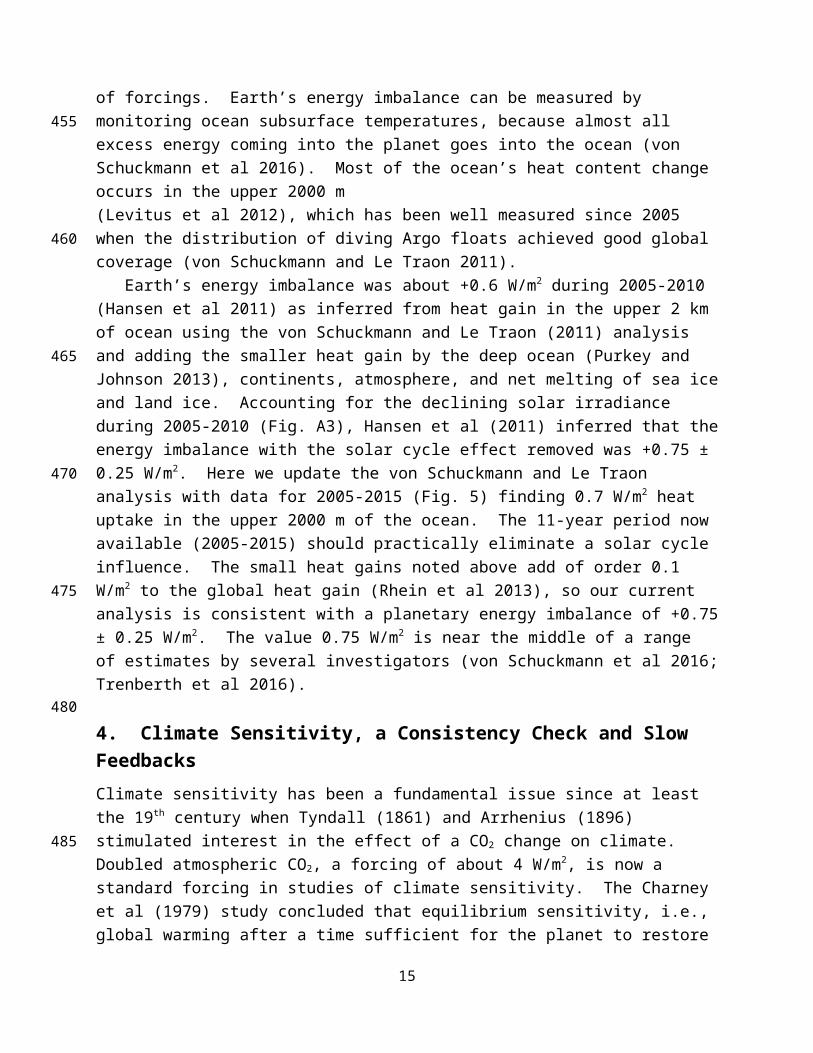
Fig. 11. (a) Atmospheric CO2 for emission scenarios of Fig. 10a. (b) Atmospheric CO2 including effect of CO2 extraction that increases linearly after 2020 (after 2015 in +2%/year case). 1 ppm is ~2.12 GtC.

7. Future CO2 for Assumed Emission ScenariosWe must model Earth’s carbon cycle, including ocean uptake of carbon, deforestation, forest regrowth and carbon storage in the soil, for the purpose of simulating future atmospheric CO2 as a function of fossil fuel emission scenario. Fortunately, the convenient dynamic-sink pulse-response function version of the well-tested Bern carbon cycle model (Joos et al 1996) does a good job of approximating more detailed models, and it produces a good match to observed industrial-era atmospheric CO2. Thus we use this relatively simple model, described elsewhere (Joos et al 1996; Kharecha and Hansen 2008 and references therein), to examine the effect of alternative fossil fuel use scenarios on the growth or decline of atmospheric CO2. For land use CO2 emissions in the historical period, we use the values labeled Houghton/2 by Hansen et al (2008), which were shown in the latter publication to yield good agreement with observed CO2. We use fossil fuel CO2 emissions data for 1850-2013 from Boden et al (2016). BP fuel consumption data for 2013-2015 is used with the fractional annual changes for each nation to allow extension of the Boden analysis through 2015. Emissions were almost flat from 2014 to 2015, due to economic slowdown and increased use of low-carbon energies, but, even if a peak in global emissions is near, substantial decline of emissions is dependent on acceleration in the transformation of energy production and use (Jackson et al 2016)..    The scenarios shown in Figs. 10a and 11a are the baseline cases without any anthropogenic CO2 removal. We illustrate five cases with CO2 removal in Fig. 11b that achieve atmospheric CO2 targets of either 350 ppm or 450 ppm in 2100, with cumulative removal amounts listed in parentheses. The rate of CO2 extraction in all cases increases linearly from zero in 2010 to the value in 2100 that achieves the atmospheric CO2 target (350 ppm or 450 ppm). The amount of CO2 that must be extracted from the system exceeds the difference between the atmospheric amount without extraction and the target amount, e.g., constant CO2 emissions and no extraction yields 546 ppm for atmospheric CO2 in 2100, but to achieve a target of 350 ppm the required extraction is 328 ppm, not 546 – 350 = 196 ppm. The well-known reason (Cao and Caldeira 2010) is that ocean out gassing increases, and vegetation productivity and ocean CO2 uptake decrease with decreasing atmospheric CO2, as explored in a wide range of Earth System models (Jones et al 2016).

15

490

495

500

505

510

515

520

8. Simulations of Global Temperature ChangeAnalysis of future climate change and policy options to alter that change must address various uncertainties. One useful way to treat uncertainty is to use results of many models and construct probability distributions (Collins et al 2013). Such distributions have been used to estimate the remaining budget for fossil fuel emissions for a specified likelihood of staying under a given global warming limit and to compare alternative policies for limiting climate forcing and global warming (Rogelj et al 2016a,b).

Our aim here is a fundamental, transparent calculation that clarifies how future warming depends on the rate of fossil fuel emissions. We use best estimates for fundamental uncertain quantities such as climate sensitivity. If these estimates are accurate, actual temperature should have about equal chances of falling higher or lower than the calculated value. Among the important uncertainties in projections of future climate forcings and climate change are climate sensitivity, the effects of ocean mixing and dynamics on the climate response function discussed below, and aerosol climate forcing. We provide all defining data so that others can easily repeat calculations with alternative choices.

We calculate global temperature change T at time t in response to any climate forcing scenario using the Green’s function (Hansen 2008)

T(t) = ʃ R(t) [dF/dt] dt (1)

where R(t) is the product of equilibrium global climate sensitivity and the dimensionless climate response function (percent of equilibrium response), dF/dt is the annual increment of net forcing, and the integration begins before human-made climate forcing is substantial. Our response function reaches 75% response in 100 years, a rate that Hansen et al (2011) conclude is representative of the real world, based on observations of Earth’s energy imbalance; this imbalance is an immediate consequence of the time required for the ocean surface temperature to respond to changing climate forcing. Our results can be exactly reproduced, or altered with alternative choices for climate forcings, climate sensitivity and response function, as we tabulate the forcings in Table S1 and the response function is exactly defined.4

We use equilibrium fast-feedback climate sensitivity ¾ °C per W/m2 (3°C for 2×CO2). This is consistent with current climate models (Collins et al 2013: Flato et al 2013) and paleoclimate evidence (Rohling et al 2012a; Masson-Delmotte et al 2013; Bindoff and Stott 2013).

CO2 is the dominant forcing in scenarios for future climate. The growth of non-CO2 GHG climate forcing is likely to be even smaller, relative to CO2 forcing, than it has been in recent decades (Fig. 9), especially if there is a strong effort to limit climate change. Indeed, recent agreement to use the Montreal Protocol (2016) to phase down emissions of minor trace gases should cause added forcing of Montreal Protocol Trace Gases (MPTGs) + Other Trace Gases (OTGs) (red region in Fig. 9) to become near zero or slightly negative, thus at least partially off-setting growth of the N2O climate forcing. Some N2O increase may be inevitable, because its emissions are largely associated with food production, and population is not expected to stabilize before mid-century at the earliest (Ciais et al 2013; Kroeze and Bouwman 2011).

4We use the “intermediate” response function in Fig. 5 of Hansen et al. (2011), which gives best agreement with Earth’s energy imbalance. Fractional response is 0.15, 0.55, 0.75 and 1 at years 1, 10, 100 and 2000 with these values connected linearly in log (year), cf. Fig. 5 of Hansen et al (2011).

16

525

530

535

540

545

550

555

560

Fig. 12. Climate forcings used in our climate simulations; Fe is effective forcing, as discussed in connection with Fig. 4. (a) Future GHG forcing uses four alternative fossil fuel emission growth rates. (b) GHG forcings are altered based on CO2 extractions of Fig. 11.

The net effect of nitrogen emissions is complex because of both diminishing and amplifying feedbacks (Kroeze and Bouwman 2011), e.g., fertilizers can increase uptake of carbon by the biosphere and affect tropospheric O3, but it is expected that more efficient use of fertilizers can reduce emissions and N2O growth (Liu and Zhang 2011). CH4 is responsible for the largest non-CO2 GHG forcing, with potential to significantly exacerbate or alleviate the magnitude of global warming, so we address the range of CH4 possibilities in Section 11. Here we use RCP6.0 for the non-CO2 GHGs, a scenario in which warming by these gases, compared to CO2, is small.

We take tropospheric aerosol plus surface albedo forcing as −1.2 W/m2 in 2015, presuming the aerosol and albedo contributions to be −1 W/m2 and −0.2 W/m2, respectively. We assume a small increase this century as global population rises and increasing aerosol emission controls in emerging economies tend to be offset by increasing development elsewhere, so aerosol + surface forcing is −1.5 W/m2 in 2100. The temporal shape of the historic aerosol forcing curve (Table S1) is from Hansen et al (2011), which in turn was based on the Novakov et al (2003) analysis of how aerosol emissions have changed with technology change.

Historic stratospheric aerosol data (Table S1, annual version), an update of Sato et al (1993), include moderate 21st century aerosol amounts (Bourassa et al 2012). Future aerosols, for realistic variability, include three volcanic eruptions in the rest of this century with properties of the historic Agung, El Chichon and Pinatubo eruptions, and a background stratospheric aerosol forcing −0.1 W/m2. This leads to mean stratospheric aerosol climate forcing −0.25 W/m2 for the 21st century, similar to the prior century. Reconstruction of historical solar forcing (Coddington et al 2015; Kopp et al 2016), based on data in Fig. A3, is extended with an 11-year cycle.

17

565

570

575

580

585

Fig. 13. Simulated global temperature for forcings of Fig. 12. Observations as in Fig. 2. Gray area is 2σ (95% confidence) range for centennially-smoothed Holocene maximum, but there is further uncertainty about the magnitude of the Holocene maximum, as noted in the text and discussed by Liu et al (2014).

Individual and net climate forcings for the several fossil fuel emission reduction rates are shown in Fig. 12a,c. Scenarios with linearly growing CO2 extraction at rates required to yield 350 or 450 ppm airborne CO2 in 2100 are in Fig. 12b,d. These forcings and the assumed climate response function define expected global temperature for the entire industrial era (Fig. 13).

A stark summary of alternative futures emerges from Fig. 13. If emissions grow 2%/ year, modestly slower than the 2.6%/year growth of 2000-2015, warming reaches ~3°C by 2100. Warming is close to 2°C if emissions are constant until 2100. Furthermore, both scenarios launch Earth onto a course of more dramatic change well beyond the initial 2-3°C global warming, because: (1) warming continues beyond 2100 as the planet is still far from equilibrium with the climate forcing, and (2) warming of 2-3°C would unleash strong slow feedbacks, including melting of ice sheets and increases of GHGs, thus continuing growing climate change. Reducing global emissions at a rate of 3%/year (or more steeply) maintains global warming at less than 1.5°C above preindustrial, but the temperature at the end of the century continues to be 0.5°C or more above the prior Holocene maximum with consequences that are difficult to foresee, especially due to the likelihood of initiating substantial amplifying slow feedbacks.

Desire to avoid slow feedbacks, including ice sheet shrinkage and sea level rise, spurs the need to get global temperature back into the Holocene range. This goal needs to be achieved on the time scale of a century or less, as paleoclimate evidence indicates that the response time of sea level to climate change is 1-4 centuries (Grant et al 2012, 2014) for natural climate change, and it is unlikely that the response would be slower to a stronger, more rapid human-made climate forcing. The scenarios that reduce CO2 to 350 ppm succeed in getting temperature back close to the Holocene maximum by 2100 (Fig. 13b), but they require extractions of atmospheric CO2 that range from 72 ppm in the scenario with 6%/year emission reductions to 768 ppm in the scenario with +2%/year emission growth.

Scenarios ranging from constant emissions to +2%/year emissions growth can be made to yield 450 ppm in 2100 via extraction of 160-600 ppm of CO2 from the atmosphere (Fig. 12b). However, these scenarios still yield warming more than 1.5°C above the preindustrial level (more than 1°C above the early Holocene maximum). Consequences of such warming and the plausibility of extracting such huge amounts of atmospheric CO2 are considered below.

18

590

595

600

605

610

615

620

9. CO2 Extraction: Plausibility and CostThe above calculations show the need for extraction of CO2 from the air, also called negative emissions, in addition to reducing emissions of GHGs. A goal of 100 GtC (47 ppm CO2) extraction in the 21st century was chosen by Hansen et al (2013), because it is comparable to net emissions from historic deforestation and land use (Ciais et al 2013), and thus it is likely to be about as much as can be achieved via relatively natural reforestation and afforestation (Canadell and Raupach 2008) and improved agricultural practices that increase soil carbon (Smith 2016).

We differentiate between the limited carbon that can be extracted from the air by improved agricultural and forestry practices and additional “technological extraction” by intensive negative emission technologies that might be used to remediate overshoot of the CO2 level needed to assure an acceptable long-term climate state. We assume that improved practices will aim at optimizing agricultural and forest carbon uptake via relatively natural approaches, compatible with delivering a range of ecosystem services from the land (Smith 2016; Smith et al 2016) In contrast, proposed technological extraction and storage of CO2 does not have co-benefits and remains unproven at relevant scales (NRC 2015). Improved practices have local benefits in agricultural yields and forest products and services (Smith et al 2016), which may help minimize net costs. Developed countries recognize a financial obligation to less developed countries that have done little to cause climate change (Paris Agreement 2015)5. We suggest that at least part of developed country support should be channeled through an agricultural and forestry program, with continual evaluation and adjustment to reward and encourage progress (Bustamante et al 2014). Non-CO2 GHGs could be included in the improved practices program. We do not estimate the program cost, but we assume that such a program will be carried out, if there is to be hope of stabilizing climate. Thus the costs we estimate for additional technological extraction of CO2 are a minimum cost.

Here we first reexamine the question of whether a concerted global effort on carbon storage in forests and soil might have potential to provide a carbon sink substantially larger than 100 GtC this century. Smith et al. (2016) estimate that reforestation and afforestation together have carbon storage potential of about 1.1 GtC/year. However, as forests mature, their uptake of atmospheric carbon decreases (termed “sink saturation”), thereby limiting CO2 drawdown. Taking 50 years as the average time for tropical, temperate and boreal trees to experience sink saturation yields 55 GtC as the potential storage in forests this century.

Smith (2016) shows that soil carbon sequestration and soil amendment with biochar compare favorably with other negative emission technologies with less impact on land use, water use, nutrients, surface albedo, and energy requirements, but understanding of and literature on biochar are limited (NRC 2015). Smith concludes that soil carbon sequestration has potential to store 0.7 GtC/year. However, as with carbon storage in forest, there is a saturation effect. A commonly used 20-year saturation time (IPCC 2006) would yield storage of 14 GtC soil carbon storage, while an optimistic 50-year saturation time would yield 35 GtC. Use of biochar to improve soil fertility provides additional carbon storage with potential rate as high as 0.7-1.8 GtC/year (Woolf et al 2010; Smith 2016). Larger industrial-scale biochar carbon storage is conceivable, but belongs in the category of intensive negative emission technologies, discussed 5 Another conceivable source of financial support for CO2 drawdown might be legal settlements with fossil fuel companies, analogous to penalties that courts have imposed on tobacco companies, but with the funds directed to the international “improved practices” program.

19

625

630

635

640

645

650

655

660

15

below, whose environmental impacts and costs require scrutiny. We conclude that 100 GtC is an appropriate estimate for potential carbon extraction via an ambitious concerted global-scale effort to improve agricultural and forestry practices with carbon drawdown as a prime objective.

Copious CO2 extraction is conceivable via other intensive negative emission technologies, including (1) burning of biofuels in power plants with capture and sequestration of resulting CO2 (Creutzig et al 2015), and (2) direct air capture of CO2 and sequestration (Keith 2009; NRC 2015), and (3) grinding and spreading of minerals such as olivine to enhance the geological weathering process (Taylor et al 2016). However, energy, land and water requirements of these technologies impose economic and biophysical limits on CO2 extraction (Smith et al 2016).

The popular concept of bioenergy with carbon capture and storage (BECCS) requires large areas, high fertilizer and water use, and may compete with other vital land use such as agriculture (Smith, 2016). Costs estimates are ~$150-350/tC for crop-based BECCS (Smith et al 2016).

Direct air capture has less area and water needs than BECCS and no fertilizer requirement, but it has high energy use, has not been demonstrated at scale, and cost estimates exceed those of BECCS (Socolow et al 2011; Smith et al 2016). Keith et al (2006) have argued that, with strong research and development support and industrial-scale pilot projects sustained over decades, it may be possible to achieve costs ~$200/tC, thus comparable to BECCS costs; however other assessments are higher, reaching $1400-3700/tC (NRC 2015). Carbon capture and storage (CCS) from a stream of nearly 100 percent CO2 at fossil fuel burning sites is more efficient and thus less expensive than direct air capture, but CCS at power plants is properly included in our scenarios as one of the mechanisms competing to achieve phase-down of fossil fuel emissions, along with energy efficiency, renewable energies, and nuclear power.

Enhanced weathering via soil amendment with crushed silicate rock is a candidate negative emission technology that also limits coastal ocean acidification as chemical products liberated by weathering increase land-ocean alkalinity flux (Kohler et al 2010; Taylor et al 2016). If two-thirds of global croplands were amended with basalt dust, as much as 2-5 GtC/year might be extracted, depending on application rate (Taylor et al 2016), but energy costs from mining, grinding and spreading likely reduce this by 10-25% (Moosdorf et al 2014). Although such large-scale enhanced weathering is speculative, there are potential co-benefits for temperate and tropical agroecosystems that could affect its practicality, and may put some enhanced weathering into the category of improved agricultural and forestry practices. Benefits include fertilizing of crops that increases yield and reduces use and cost of other fertilizers, increasing crop protection from insect herbivores and pathogens thus decreasing pesticide use and cost, neutralizing soil acidification to improve yield, and suppression of GHG (N2O and CO2) emissions from soils (Edwards et al 2016; Kantola et al 2016). Cost of enhanced weathering might be reduced by deployment with reforestation and afforestation and with crops used for BECCS.

For cost estimates, we first consider restoration of airborne CO2 to 350 ppm in 2100 (Fig. 11b), which would keep global warming below 1.5°C and bring global temperature back close to the Holocene maximum by end-of-century (Fig. 13b). This scenario keeps the temperature excursion above the Holocene level small enough and brief enough that it has the best chance of avoiding ice sheet instabilities and multi-meter sea level rise (Hansen et al 2016). If fossil fuel emission phasedown of 6%/year had begun in 2013, as proposed by Hansen et al (2013), this scenario would have been achieved via the 100 GtC carbon extraction from improved agricultural and forestry practices.

20

665

670

675

680

685

690

695

700

705

Now, with assumption that global emissions will be comparable to today’s level through 2020, Figs. 11b and 13b show that 6%/year emissions reduction starting in 2021 leaves a requirement to extract 72 ppm CO2 (153 GtC) from the air during this century. Emission reductions of 3%/year leave a requirement of extracting 112 ppm CO2 (Fig. 13b) by 2100. Constant emissions and +2%/year emissions growth would require extractions of 328 and 768 ppm CO2 to reach 350 ppm in 2100.

The lowest cost is for the case of 6%/year emissions reduction. We assume that 100 GtC will be stored in the biosphere via improved agricultural and forestry practices. We do not mean to diminish the magnitude or cost of this task, but we must assume that it will occur if climate change impacts are to be minimized, and further we expect that developed countries will recognize their obligations to provide assistance required to achieve success.

The remaining 53 GtC, at the rate $150-350/tC estimated for BECCS and other intensive negative emission technologies (Fig. 3f of Smith et al 2016), would cost $8-18.5 trillion, thus $100-230 billion per year if spread uniformly over 80 years. In contrast, continued high emissions, say between constant emissions and +2%/year, require extraction of 695-1628 GtC, which corresponds to $104-570 trillion dollars or $1.3-7 trillion dollars per year over 80 years.6 Such extraordinary cost, along with the land area, fertilizer and water requirements (Smith et al 2016) suggest that, rather than the world being able to buy its way out of climate change, continued high emissions may force humanity to largely live with the climatic consequences.

10. Climate Forcing Contribution of Non-CO2 GHGsGHG climate forcing is surging, not declining, the annual rate having increased more than 20% in just the past five years (Fig. A5). This recent surge in the growth rate of the GHG climate forcing is led by increasing growth of CH4, but CO2 is by far the largest cause of continued growth of the GHG climate forcing (Fig. 9). Given the difficulty and cost of reducing CO2, we must ask about the alternative of reducing non-CO2 GHGs. Could realistic reductions of these other gases substantially alter the CO2 abundance required to meet a target climate forcing?

Methane (CH4) is the largest climate forcing other than CO2 (Fig. 3). The CH4 atmospheric /lifetime is only about 10 years (Prather et al 2012), so there is potential to reduce this climate forcing rapidly if CH4 sources are reduced. Our climate simulations, employing RCP6.0 for non-CO2 gases, make an optimistic assumption that future CH4 , after a moderate increase in the next few decades, will decrease from its present ~1800 ppb to 1650 ppb in 2100, yielding a forcing −0.1 W/m2. RCP2.6 makes a more optimistic assumption: that CH4 will decline monotonically to 1250 ppb in 2100, yielding a forcing −0.3 W/m2 (relative to today’s 1800 ppb CH4), based on radiation equations identified in section 6.

6 For reference, the United Nations global peacekeeping budget is about $10B/year. National military budgets are larger: the 2015 USA military budget was $596B and the global military budget was $1.77 trillion (SIPRI 2016).

21

710

715

720

725

730

735

740

Fig. 14. Comparison of observed CH4 and N2O amounts and RCP scenarios. RCP 6.0 and 4.5 scenarios for N2O overlap. Observations are from NOAA/ESRL Global Monitoring Division.

Actual atmospheric CH4 abundance (Fig. 14) is diverging on the high side from these optimistic scenarios. The downward offset (~20 ppb) of CH4 scenarios relative to observations (Fig. 14) is due to the fact that RCP scenarios did not include a data adjustment that was made in 2005 to match a revised CH4 standard scale (E. Dlugokencky, priv comm). In addition, observed CH4 is increasing more rapidly than in most scenarios.

Carbon isotopes provide a valuable constraint on which CH4 sources7 contribute to the CH4 growth resurgence in the past decade (Fig. 7). Specifically, Schaefer et al (2016) conclude that the growth was primarily biogenic, thus not fossil fuel, and located outside the tropics, most likely ruminants and rice agriculture. Such an increasing biogenic source is consistent with effects of increasing population and dietary changes (Tilman and Clark 2014). These sources potentially could be mitigated [by changing rice growing methods (Epule et al 2011) and inoculating ruminants (Eckard et al, 2010; Beil 2015)], but that would require widespread adoption of new technologies at the farmer level. Concerning fossil fuels, it is feasible to reduce CH4 leaks, yet enhanced shale gas extraction of CH4 may yield even greater leakage (Caulton et al., 2014; Petron et al., 2014; Howarth, 2015).

Slow climate feedbacks could increase CH4 because natural emissions from methane hydrates, permafrost and natural wetlands8 are expected to increase in response to global warming (O’Connor et al 2010). On the other hand, as yet there is little evidence for substantial emissions from hydrates or permafrost (Warwick et al., 2016). Predicting such emissions has large uncertainty, because drought conditions eliminate wetland CH4 emissions (while greatly increasing CO2 release from soil carbon), and, in addition, CH4 created in anoxic zones is mostly oxidized in the water column before reaching the atmosphere (Reeburgh, 2007).

All reasonable effort to reduce methane is appropriate, recognizing that its mitigation effort will be different than that for fossil fuel CO2 in that it should include a focus on agriculture in developing countries with adoption of new practices and technology at the farm level. However, given increasing global population and global warming “in the pipeline,” there is an underlying 7 Estimated human-caused CH4 sources (Ciais et al., 2013) are: fossil fuels (29%), biomass/biofuels (11%), Waste and landfill (23%), ruminants (27%) and rice (11%) 8 Wetlands compose a majority of natural CH4 emissions and are estimated to be equivalent to about 36% of the anthropogenic source (Ciais et al., 2013)

22

745

750

755

760

765

770

20

tendency for greater emissions. The current CH4 increases (Fig. 14a) show that the mitigation paths envisaged with RCP scenarios projecting methane decreases are not close to present reality. Nevertheless, it is plausible that human-caused emissions could achieve a pathway to a moderate reduction of CH4 forcing in 2100, but it seems unlikely that the reduction could be larger than of the order of 0.1 W m-2.

There is less leverage with N2O, whose growth is exceeding all scenarios (Fig. 14b). Major quantitative gaps remain in our understanding of the nitrogen cycle (Kroeze and Bouwman 2011), but fertilizers are clearly a principal cause of N2O growth (Röckmann and Levin2005; Park et al 2012). More efficient use of fertilizers could reduce N2O emissions, but considering the scale of global agriculture, and the fact that fixed N is an inherent part of feeding people, there will be pressure for continued emissions at least comparable to present emissions. In contrast, agricultural CH4 emissions are inadvertent and not core to food production. Given the current imbalance [emissions exceeding atmospheric losses by about 30% (Prather et al., 2012)] and the long N2O atmospheric lifetime (116 ± 9 years; Prather et al 2015) it is nearly inevitable that N2O will continue to increase this century, even if emissions growth is checked. There can be no expectation of an N2O decline that offsets the need to reduce CO2.

The Montreal Protocol has been a success in stifling and even reversing the growth of trace gases that can destroy ozone and cause global warming (Prather et al 1996; Newman et al 2009). Amendments to this protocol to achieve phasedown of additional gases are important, but mainly for the objective of limiting the growth of these trace gas climate forcings rather than with an expectation of obtaining a large net reduction of climate forcing by MPTGs + OTGs (Fig. 3).

11. DiscussionWe conclude that the world has already overshot targets for atmospheric temperature and greenhouse gas amount required to maintain a safe long-term environment for humanity and assure the well-being of young people and future generations. Earth’s paleoclimate history tells us that, if we wish to avoid locking in multi-meter sea level rise with loss of functionality of most coastal cities (Clark et al 2016), our target should be to keep global temperature close to the Holocene range, which requires an absolute reduction in current GHG climate forcing and global temperature.

Thus we infer an urgent need for both (1) rapid phasedown of fossil fuel emissions, and (2) actions that draw down atmospheric CO2 and, at minimum, eliminate net growth of non-CO2 climate forcings. These tasks are formidable and are not now being pursued effectively.

Although economic and political analysis is outside the scope of this paper, our conclusion that the world has already overshot appropriate targets is sufficiently grim to compel us to point out that pathways minimizing climate impacts are feasible and have other benefits. The underlying policy required to spur rapid reduction of fossil fuel emissions is a transparent steadily rising carbon fee that makes fossil fuels include their costs to society (Ackerman and Stanton 2012; Hsu 2011; Hansen 2014), which encourages energy conservation (reduced consumption), energy efficiency, and technology development of carbon-free energy. A rising global carbon fee, which could be achieved by agreement of a few major powers (Hsu 2011), is the crucial underlying policy needed to spur private investment, innovations and consumer choices, but it does not obviate the need for government energy planning, energy efficiency and pollution regulations, and support for energy research and development.

23

775

780

785

790

795

800

805

810

815

Governments have shown the ability to achieve high rates of emissions reduction, e.g., Peters et al (2013) note that Belgium, France and Sweden achieved emission reductions of 4-5%/year sustained over 10 or more years in response to the oil crisis of 1973. These rates were primarily a result of nuclear power build programs, which historically has been the fastest route to carbon-free energy (Fig. 2 of Cao et al 2016). Peters et al also note that a continuous shift to natural gas led to sustained reductions of 1-2%/year in the UK in the 1970s and in the 2000s, 2%/year in Denmark in 1990-2000s, and 1.4%/year in the USA since 2005. None of these examples were aided by the broad economy-wide effect of a rising carbon fee, although high oil prices in the 1970s partially simulated that effect. What is needed to achieve rates presently demanded by the climate crisis is a combination of a rising carbon fee along with government support of technological advances, which has historically received the smallest share of total research budgets in OECD countries.

Our scenarios show that, in addition to CO2 emission phase-out, there must be large CO2 extraction from the air and a net halt of growth of non-CO2 GHG climate forcings. Success with both CO2 extraction and non-CO2 GHG controls requires a major role for developing countries. Ancillary benefits of the agricultural and forestry practices needed to achieve CO2 drawdown, such as improved soil fertility, advanced agricultural practices, forest products, and species preservation, are of interest to all nations. Developed nations have a recognized obligation to assist nations that have done little to cause climate change yet suffer some of the largest climate impacts. If economic assistance is made partially dependent on verifiable success in carbon drawdown and non-CO2 mitigation, this will provide incentives that maximize success in carbon storage. Similar considerations apply to incentives for reducing trace gas emissions, and, as we have discussed, some activities such as soil amendments that enhance weathering might be designed to support both CO2 and other GHG drawdown.

Considering our conclusion that the world has overshot the appropriate target for global temperature, and the difficulty and perhaps implausibility of negative emissions scenarios, we would be remiss if we did not point out the potential contribution of demand-side mitigation that can be achieved by individual actions as well as by government policies. Numerous studies (e.g. Hedenhus et al 2014; Popp et al 2010) have shown that reduced ruminant meat and dairy products is needed to reduce GHG emissions from agriculture, even if technological improvements increase food yields per unit farmland. Such climate-beneficial dietary shifts have also been linked to co-benefits that include improved sustainability and public health (Bajzelj et al 2014; Tilman and Clark 2014). Similarly, Working Group 3 of IPCC (2014) finds “robust evidence and high agreement” that demand-side measures in the agriculture and land use sectors, especially diet shifts, reduced food waste and changes in wood consumption have substantial mitigation potential, but they remain under-researched and poorly quantified.

If rapid emission reductions are initiated soon, it is still possible that at least a large fraction of required CO2 extraction can be achieved via relatively natural agricultural and forestry practices with other benefits. On the other hand, if large fossil fuel emissions are allowed to continue, the scale and cost of industrial CO2 extraction, occurring in conjunction with a deteriorating climate with growing economic effects, may become unmanageable. Simply put, the burden placed on young people and future generations may become too heavy to bear.Appendix A: Additional figures and tables

24

820

825

830

835

840

845

850

855

Fig. A1. CO2 emissions from fossil fuel use and cement manufacture, based on data of Boden et al (2016) through 2013, with results extended using BP(2016) energy consumption data. (a) is log scale and (b) is linear. Growth rates r in (a) for an n year interval from (1+r)n with end-year amount the mean for three years to minimize noise.

A1. Fossil Fuel CO2 Emissions

CO2 emissions from fossil fuels in 2015, based on preliminary data from BP (2016), were only slightly higher than in 2014 (Fig. A1). Such slowdowns are common, and usually reflect the global economic situation. Given rising global population and the fact that many nations, including the soon-to-be-most-populous India, are still at early stages of development, the potential exists for continued growth of emissions. Fundamental changes in energy technology will be needed if the world is to rapidly change energy course and phase down fossil fuel emissions.

A2. Temperature Data and Analysis Method

We use the current Goddard Institute for Space Studies global temperature analysis (GISTEMP), which is the analysis method described by Hansen et al. [2010] but with updated input data. The analysis combines data from three sources: (1) monthly mean meteorological station data of the Global Historical Climatology Network (GHCN) described by Peterson and Vose [1997] and Menne et al. [2012], (2) monthly mean data from Antarctic research stations of the Scientific Committee on Antarctic Research (SCAR), as reported by the SCAR Reference Antarctic Data for Environmental Research project (http://www.antarctica.ac.uk/met/READER), and (3) ocean surface temperature measurements from the NOAA Extended Reconstructed Sea Surface Temperature (ERSST) [Smith et al., 2008; Huang et al., 2015].

25

860

865

870

875

880

885

Fig. A2a. Global surface temperature (12-month running mean) relative to 1951-1980 in the GISTEMP analysis, comparing the current analysis using NOAA ERSST.v4 for sea surface temperature with results using the prior ERSST.v3b.

The present analysis uses GHCN.v3.3.0 [Menne et al., 2012] for land data and ERSST.v4 for sea surface temperature [Huang et al., 2015]. Update from GHCN.v2 used in our 2010 analysis to GHCN.v3 had negligible effect on global temperature change over the past century (see graph on http://www.columbia.edu/~mhs119/Temperature/GHCN_V3vsV2/). However, the adjustments to SST to produce ERSST.v4 have a noticeable effect, especially in the period 1939-1945, as shown by the difference between the two data sets (lower graph in Fig. A2a). This change is of interest mainly because it increases the magnitude of an already unusual global temperature fluctuation in the 1940s, making the 1939-1945 global temperature maximum even more pronounced than it was ERSST.v3 data. Thompson et al. [2008] show that two natural sources of variability, the El Niño/Southern Oscillation and (possibly related) unusual winter Arctic warmth associated with advection over high Northern Hemisphere latitudes, partly account for global warmth of 1939-1945, and they suggest that the sharp cooling after 1945 is a data flaw, due to a rapid change in the mix of data sources (bucket measurements and engine room intake measurements) and a bias between these that is not fully accounted for.

26

890

895

900

905

Fig. A2b. Temperature anomalies in three periods relative to 1951-1980 comparing results obtained using ERSST.v3b (left column), ERSST.v4 (center column), and their difference (right column).

Huang et al. [2015] justify the changes made to obtain version 4 of ERSST, the changes including more complete input data in ICOADS Release 2.5, buoy SST bias adjustments not present in version 3, updated ship SST bias adjustments using Hadley Nighttime Marine Air Temperature version 2 (HadNMat2), and revised low-frequency data filling in data sparse regions using nearby observations. ERSST.v4 is surely an improvement in the record during the past half century when spatial and temporal data coverages are best. On the other hand, the largest changes between v3 and v4 are in 1939-1945, coinciding with World War II and changes in the mix of data sources. Several hot spots appear in the Southern Hemisphere ocean during WW II in the v4 data, and then disappear after the war (Fig. A2b). These hot spots coincide with the locations of large SST changes between v3 and v4 (Fig. A2b), which leads us to suspect that the magnitude of the 1940s global warming maximum (Fig. 2) is exaggerated; i.e., it is partly spurious. We suggest that this warming spike warrants scrutiny in the next version of the SST analysis. However, the important point is that these data adjustments and uncertainties are small in comparison with the long-term warming. Adjustments between ERSST.v3b and ERSST.v4 increase global warming over the period 1950-2015 by about 0.05°C, which is small compared with the ~1°C global warming during that period. The effect of the adjustments on total global warming between the beginning of the 20th century and 2015 is even smaller (Fig. A2a).

27

910

915

920

925

Fig. A3. Solar irradiance and sunspot number in the era of satellite data. Left scale is the energy passing through an area perpendicular to Sun-Earth line. Averaged over Earth’s surface the absorbed solar energy is ~240 W/m2, so the full amplitude of the measured solar variability is ~0.25 W/m2.

A3. Solar Irradiance

Solar irradiance has been measured from satellites since the late 1970s. Fig. A3 is a composite of several satellite-measured time series. Data through 28 February 2003 are an update of Frohlich and Lean (1998) obtained from Physikalisch Meteorologisches Observatorium Davos, World Radiation Center. Subsequent update is from University of Colorado Solar Radiation & Climate Experiment (SORCE). Historical total solar irradiance reconstruction is available at http://lasp.colorado.edu/home/sorce/data/tsi-data/ Data sets are concatenated by matching the means over the first 12 months of SORCE data. Monthly sunspot numbers support the conclusion that the solar irradiance in the current solar cycle is significantly lower than in the three preceding solar cycles.

The magnitude of the change of solar irradiance from the prior solar cycle to the current solar cycle is of the order of −0.1 W/m2, which is not negligible but is small compared with greenhouse gas climate forcing. On the other hand, the variation of solar irradiance from solar minimum to solar maximum is of the order of 0.25 W/m2, so the high solar irradiance in 2011 -2015 contributes to the increase of Earth’s energy imbalance between 2005-2010 and 2010-2015.

28

930

935

940

945

Fig. A4. Simulated global temperature with historical climate forcings to 2000 followed by the alternative scenario. Historical climate forcings are discussed in the main text.

A4. Alternative Scenario

Simulated global temperature for the climate forcings of the “alternative scenario” discussed in Section 6 are shown in Fig. A4. Climate model, with sensitivity 3°C for doubled CO2, is the same as used for Fig. 13.

Fig. A5. Recent growth rate of total GHG climate forcing; see Fig. 9 for individual gases.

A5. Growth Rate of Total GHG Climate Forcing

In the past several years the growth rate of climate forcing by GHGs has accelerated sharply, in contrast to most scenarios, which presumed that the GHG climate forcing would be declining. Ozone is not well-mixed, so its changes are not well-measured and are not fully accounted for in Fig.5. However, the effective CH4 forcing, which is included, includes about half of the tropospheric O3 change.

29

950

955

960

965

-----------------------------------------------------------------------------Table A1. Effective Forcing (W/m2) Relative to 1850 except Volcanic Aerosols-----------------------------------------------------------------------------Year CO2 CH4* CFCs N2O O3

$ TA+SA Volcano Solar Net-----------------------------------------------------------------------------1850 0.000 0.000 0.000 0.000 0.000 0.000 -0.083 0.000 -0.0831860 0.024 0.012 0.000 0.004 0.004 -0.029 -0.106 0.032 -0.0591870 0.048 0.025 0.000 0.007 0.009 -0.058 -0.014 0.048 0.0651880 0.109 0.039 0.000 0.010 0.014 -0.097 -0.026 -0.049 -0.0011890 0.179 0.054 0.000 0.013 0.018 -0.146 -0.900 -0.070 -0.8501900 0.204 0.073 0.001 0.016 0.023 -0.195 -0.040 -0.063 0.0181910 0.287 0.109 0.002 0.020 0.026 -0.250 -0.072 -0.043 0.0791920 0.348 0.150 0.003 0.027 0.032 -0.307 -0.215 -0.016 0.0221930 0.425 0.194 0.004 0.035 0.036 -0.364 -0.143 0.014 0.2001940 0.494 0.232 0.005 0.041 0.045 -0.424 -0.073 0.037 0.3561950 0.495 0.274 0.009 0.049 0.056 -0.484 -0.066 0.055 0.3871960 0.599 0.342 0.027 0.057 0.078 -0.621 -0.106 0.102 0.4781970 0.748 0.433 0.076 0.071 0.097 -0.742 -0.381 0.093 0.3951980 0.976 0.532 0.185 0.091 0.115 -0.907 -0.108 0.169 1.0541990 1.227 0.618 0.303 0.118 0.117 -0.997 -0.141 0.154 1.3992000 1.464 0.651 0.347 0.141 0.117 -1.084 -0.048 0.173 1.7612005 1.619 0.651 0.356 0.153 0.123 -1.125 -0.079 0.019 1.7162010 1.766 0.665 0.364 0.167 0.129 -1.163 -0.082 0.028 1.8742015 1.927 0.684 0.373 0.183 0.129 -1.199 -0.100 0.137 2.134-----------------------------------------------------------------------------#CH4:CH4-induced changes of tropospheric O3 and stratospheric H2O are included.$O3 half of tropospheric O3 forcing + stratospheric O3 forcing from IPCC (2013)Annual data are available in a longer version of the table available at http://www.columbia.edu/~mhs119/Burden/.

-----------------------------------------------------------------------------Table A2. Effective Forcing (W/m2) Relative to 1850 except Volcanic Aerosols-----------------------------------------------------------------------------Year CO2 #CH4 CFCs N2O $O3 TA+SA Volcano Solar Net-----------------------------------------------------------------------------2016 1.942 0.654 0.367 0.180 0.130 -1.207 -0.100 0.097 2.0622020 2.074 0.658 0.373 0.189 0.130 -1.234 -0.100 -0.008 2.0822030 2.347 0.663 0.343 0.212 0.130 -1.296 -1.057 -0.008 1.3352040 2.580 0.688 0.301 0.238 0.123 -1.350 -0.100 0.027 2.5072050 2.803 0.717 0.267 0.271 0.117 -1.396 -0.100 0.062 2.7412060 3.017 0.740 0.243 0.302 0.111 -1.433 -1.208 0.097 1.8702070 3.222 0.753 0.229 0.337 0.105 -1.462 -0.100 0.132 3.2152080 3.421 0.741 0.215 0.367 0.098 -1.484 -0.100 0.167 3.4252090 3.614 0.676 0.199 0.401 0.091 -1.495 -1.240 0.167 2.4132100 3.801 0.580 0.191 0.428 0.085 -1.500 -0.100 0.167 3.652-----------------------------------------------------------------------------#CH4: CH4-induced changes of tropospheric O3 and stratospheric H2O are included$O3: Half of tropospheric O3 forcing + stratospheric O3 forcing from IPCC 2013Annual data are available in a longer version of the table available at http://www.columbia.edu/~mhs119/Burden/.

30

970

975

980

985

990

995

1000

1005

1010

1015

AcknowledgmentsSupport of the Climate Science, Awareness and Solutions program has been provided by the Durst family, the Grantham Foundation for Protection of the Environment, Jim and Krisann Miller, Gary Russell, Gerry Lenfest, the Flora Family Foundation, Elisabeth Mannschott, Alexander Totic and Hugh Perrine, which is gratefully acknowledged. DJB acknowledges funding through a Leverhulme Trust Research Centre Award (RC-2015-029). EJR acknowledges support from Australian Laureate Fellowship FL12 0100050

We appreciate the generosity, with data and advice, of Tom Boden, Ed Dlugokencky and Steve Montzka.

The authors declare that they have no conflicts of interest.

References

Abram, N. J., McGregor, H. V., Tierney, J. E., Evans, M. N., McKay, N. P., Kaufman, D. S., and PAGES 2k Consortium: Early onset of industrial-era warming across the oceans and continents, Nature, doi:10.1038/nature19082, 2016.

Ackerman, F. and Stanton, E. A.: Climate risks and carbon prices: revising the social cost of carbon, Economics E-journal 6 2012—10.5018/economics-ejournal.ja.2012—10, 2012.

Anderson, K.: Talks in the city of light generate more heat, Nature, 528, 437, 2015.

Andrews, T., Gregory, J., Webb, M., and Taylor, K.: Forcing, feedbacks and climate sensitivity in CMIP5 coupled atmosphere-ocean climate models, Geophys Res Lett, 39(9), L09712, 2012.

Arrhenius, S.: On the influence of carbonic acid in the air upon the temperature on the ground, Phil Mag, 41, 237-276, 1896.

Bakker, P. and Renssen, H.: Last interglacial model-data mismatch of thermal maximum temperatures partially explained, Clim Past, 10, 1633-1644, 2014.

Bajzelj, B., Richards, K. S., Allwood, J. M., Smith, P., Dennis, J. S., Curmi, E., and Gilligan, C. A.: Importance of food-demand management for climate mitigation, Nature Clim Change, 4, 924-929, doi:10.1038/nclimate2553, 2014.

Beil, L.: Getting creative to cut methane from cows, Science News, 188(11), 22-25, 2015.

Betts, R. A., Jones, C. D., Knight, J. R., Keeling, R. F., and Kennedy, J. J.: El Nino and a record CO2 rise, Nature Clim Change, 6, 806-810, 2016.

Bindoff, N. L. and Stott, P. A.: Detection and attribution of climate change: from global to regional. In Climate Change 2013: The Physical Science Basis, edited by: Stocker, T. F., Qin, D., Plattner, G.-K., Tignor, M., Allen, S. K., Boschung, J., Nauels, A., Xia, Y., Bex, V., and Midgley, P. M., Cambridge University Press, Cambridge, United Kingdom, 2013.

Boden, T. A., Marland, G., and Andres, R. J.: Global, Regional, and National Fossil-Fuel CO2 Emissions, Carbon Dioxide Information Analysis Center, Oak Ridge National Laboratory, Oak Ridge, Tennessee USA, doi 10.3334/CDIAC/00001_V2016, 2016.

Boucher, O., Randall, D., Artaxo, P., Bretherton, C., Fiengold, G., Forster, P., Kerminen, V.-M., Kondo, Y., Liao, H., Lohmann, U., Rasch, P., Satheesh, S. K., Sherwood, S., Stevens, B., and Zhang, X. Y.: Clouds and aerosols. in Climate Change 2013: The Physical Basis, edited by: Stocker, T. F., Qin, D., Plattner, G.-K., Tignor, M., Allen, S.

31

1020

1025

1030

1035

1040

1045

1050

1055

K., Boschung, J., Nauels, A., Xia, Y., Bex, V., and Midgley, P. M., Cambridge University Press, Cambridge, United Kingdom, 2013.

Bourassa, A. E., Robock, A., Randel, W. J., Deshler, T., Rieger, L. A., Lloyd, N. D., Llewellyn, E. J., and Degenstein, D. A.: Large volcanic aerosol load in the stratosphere linked to Asian Monsoon transport, Science, 337, 78-81, 2012.

Bousquet, P., Ringeval, B., Pison, I., Dlugokencky, E. J., Brunke, E.-G., Carouge, C., Chevallier, F., Fortems-Cheiney, A., Frankenberg, C., Hauglustaine, D. A., Krummel, P. B., Langenfelds, R. L., Ramonet, M., Schmidt, M., Steele, L. P., Szopa, S., Yver, C., Viovy, N., and Ciais, P.: Source attribution of the changes in atmospheric methane for 2006-2008, Atmos Chem Phys, 11, 3689-3700, 2011.

BP: 2016 BP Statistical Review of World Energy, available at: http://www.bp.com/en/global/corporate/energy-economics/statistical-review-of-world-energy.html (last access: 23 June 2016), 2016.

Bustamante, M., Robledo-Abad, C., Harper, R., Mbow, C., Ravindranath, N.H., Sperling, F., Haberl, H., de Siqueira Pinto, A. and Smith, P.: Co-benefits, trade-offs, barriers and policies for greenhouse gas mitigation in the Agriculture, Forestry and Other Land Use (AFOLU) sector, Global Change Biology, 20, 3270–3290, doi: 10.1111/gcb.12591, 2014.

Canadell, J. G. and Raupach, M. R.: Managing forests for climate change mitigation, Science, 320, 1456-1457, 2008.

Cao, J., Cohen, A., Hansen, J., Lester, R., Peterson, P., and Xu, H.: China-U.S. cooperation to advance nuclear power, Science, 353, 547-548, 2016.

Cao, L. and Caldeira, K.: Atmospheric carbon dioxide removal: long-term consequences and commitment, Environ Res Lett, 5, doi:10.1088/1748-9326/5/2/024011, 2010.

Caulton, D. R., Shepson, P. B., Santoro, R. L., Sparks, J. P., Howarth, R. W., Ingraffea, A. R., Cambaliza, M. O. L., Sweeney, C., Karion, A., Davis, K. J., Strim, B. H., Montzka, S. A., and Miller, B. R.: Toward a better understanding and quantification of methane emissions from shale gas development, Proc Natl Acad Sci USA, 111, 6237-6242, 2014.

Charney, J. G., Arakawa, A., Baker, D., Bolin, B., Dickinson, R., Goody, R., Leith, C., Stommel, H., and Wunsch, C.: Carbon Dioxide and Climate: A Scientific Assessment, Natl Acad Sci Press, Washington, DC, USA, 33p, 1979.

Chavez, F. P., Strutton, P. G., Friederich, G. E., Feely, R. A., Feldman, G. C., Foley, D. G., and McPhaden, M. J.: Biological and chemical response of the Equatorial Pacific Ocean to the 1997-98 El Nino, Science, 286, 2126-, 1999.

Ciais, P., Sabine, C., Bala, G., Bopp, L., Brovkin, V., Canadell, J., Chhabra, A., DeFries, R., Galloway, J., Heimann, M., Jones, C., Le Quere, C., Myneni, R. B., Piao, S., and Thornton, P.: Carbon and other biogeochemical cycles. in Climate Change 2013: The Physical Basis, edited by: Stocker, T. F., Qin, D., Plattner, G.-K., Tignor, M., Allen, S. K., Boschung, J., Nauels, A., Xia, Y., Bex, V., and Midgley, P. M., Cambridge University Press, Cambridge, United Kingdom, 2013.

Clark, P. U. and Huybers, P.: Interglacial and future sea level, Nature, 462, 856-857, 2009.

Clark, P.U., Shakun, J.D., Marcott, S.A., Mix, A.C., Eby, M., Kulp, S., Levermann, A., Milne, G.A., Pfister, P.L., Santer, B.D., Schrag, D.P., Soloman, S., Stocker, T.F., Strauss, B.H., Weaver, A.J., Winkelmann, R., Archer, D., Bard, E., Goldner, A., Lambeck, K., Pierrehumbert, R.T., and Plattner, G.K.: Consequences of twenty-first-century policy for multi-millennial climate and sea-level change, Nature Clim. Change, 6, 360-369, 2016.

Coddington, O., Lean, J. L., Pilewskie, P., Snow, M., and Lindholm, D.: A solar irradiance climate data record, Bull Amer Meteorol Soc, doi:10.1175BAMS-D-14-002265.12, 2015.

32

1060

1065

1070

1075

1080

1085

1090

1095

1100

Collins, M., Knutti, R., Arblaster, J., Dufresne, J. L., Fichefet, T., Friedlingstein, P., Gao, X., Gutowski, W. J., Johns, T., Krinner, G., Shongwe, M., Tebaldi, C., Weaver, A., and Wehner, M.: Long-term climate change: Projections, commitments and irreversibility, in: Climate Change 2013: The Physical Basis, edited by: Stocker, T. F., Qin, D., Plattner, G.-K., Tignor, M., Allen, S. K., Boschung, J., Nauels, A., Xia, Y., Bex, V., and Midgley, P. M., Cambridge University Press, Cambridge, United Kingdom, 2013.

Copenhagen Accord 2009: United Nations Framework Convention on Climate Change, Draft decision available at: http://unfccc.int/meetings/copenhagen_dec_2009/items/5262.php, (last access: 9 September 2016), 2009.

Creutzig, F., Ravindranaath, N. H., Berndes, G., Bolwig, S., Bright, R., Cherubini, F., Chum, H., Corbera, E., Delucchi, M., Faaij, A., Fargione, J., Haberl, H., Heath, G., Lucon, O., Plevin, R., Popp, A., Robledo-Abad, C., Rose, S., Smith, P., Stromman, A., and Suh, S.: Bioenergy and climate change mitigation: an assessment, GCB Bioenergy, 7, 916-944, 2015.

Dai, A., Fyfe, J. C., Xie, S. P., and Dai, X.: Decadal modulation of global surface temperature by internal climate variability, Nature Clim Change, published online 13 April doi:10.1038/nclimate2605, 2015.

DeConto, R. M. and Pollard, D.: Contribution of Antarctica to past and future sea-level rise, Nature, 531, 591-597, 2016.

Dlugokencky, E. J., Nisbet, E. G., Fisher, R., and Lowry, D.: Global atmospheric methane: budget, changes and dangers, Phil Trans Roy Soc A, 369, 2058-2072, 2011.

Dlugokencky, E. J.: Global CH4 data, NOAA/ESRL, available at: www.esrl.noaa.gov/gmd/ccgg/trends_ch4/, (last access: 13 September 2016), 2016.

Dutton, A., Carlson, A. E., Long, A. J., Milne, G. A., Clark, P. U., DeConto, R., Horton, B. P., Rahmstorf, S., and Raymo, M. E.: Sea-level rise due to polar ice-sheet mass loss during past warm periods, Science, 349, 153 doi:10.1126/science.aaa4019, 2015.

Eckard, R. J., Grainger, C., and de Klein, C. A. M.: Strategies to reduce methane emissions from farmed ruminants grazing on pasture, Livestock Science, 130, 47-56, 2010.

Edwards, D. P., Lim, F., James, R. H., Pearce, C. R., Scholes, J., Freckleton, R. P., and Beerling, D. J.: Tropical agrosystems and enhanced rock weathering: potential benefits and pitfalls, Biol Lett (submitted), http://mc.manuscriptcentral.com/bl, 2016.

England, M. H., McGregor, S., Spence, P., Meehl, G. A., Timmermann, A., Cai, W., Gupta, A. S., McPhaden, M. J., Purich, A., and Santoso, A.: Recent intensification of wind-driven circulation in the Pacific and the ongoing warming hiatus, Nature Clim Change, published online 9 February, doi:10.1038/nclimate2106, 2014.

Epule, E. T., Peng, C., and Mafany, N. M.: Methane emissions from paddy rice fields: strategies towards achieving a win-win sustainability scenario between rice production and methane reduction, J Sustain Devel, 4(6), 188-196, 2011.

Flato, G., Marotzke, J., Abiodun, B., Braconnot, P., Chou, S. C., Collins, W., Cox, P., Driouech, F., Emori, S., Eyring, V., Forest, C., Gleckler, P., Guilyardi, E., Jakob, C., Kattsov, V., Reason, C., and Rummukainen, M.: Evaluation of Climate Models. In: Climate Change 2013: The Physical Science Basis, edited by: Stocker, T. F., Qin, D., Plattner, G.-K., Tignor, M., Allen, S. K., Boschung, J., Nauels, A., Xia, Y., Bex, V., and Midgley, P. M., Cambridge University Press, Cambridge, United Kingdom, 2013.

Friedlingstein, P., Andrew, R. M., Rogelj, J., Peters, G. P., Canadell, J. G., Knutti, R., Luderer, G., Raupach, M. R., Schaeffer, M., van Vuuren, D. P., and Le Quere, C.: Persistent growth of CO2 emissions and implications for reaching climate targets, Nat Geosci, 1, 457-461, 2014.

Frohlich, C. and Lean, J.: The Sun’s total irradiance: cycles and trends in the past two decades and assoiated climate change uncertainties, Geophys Res Lett, 25, 4377-4380, 1998.

33

1105

1110

1115

1120

1125

1130

1135

1140

1145

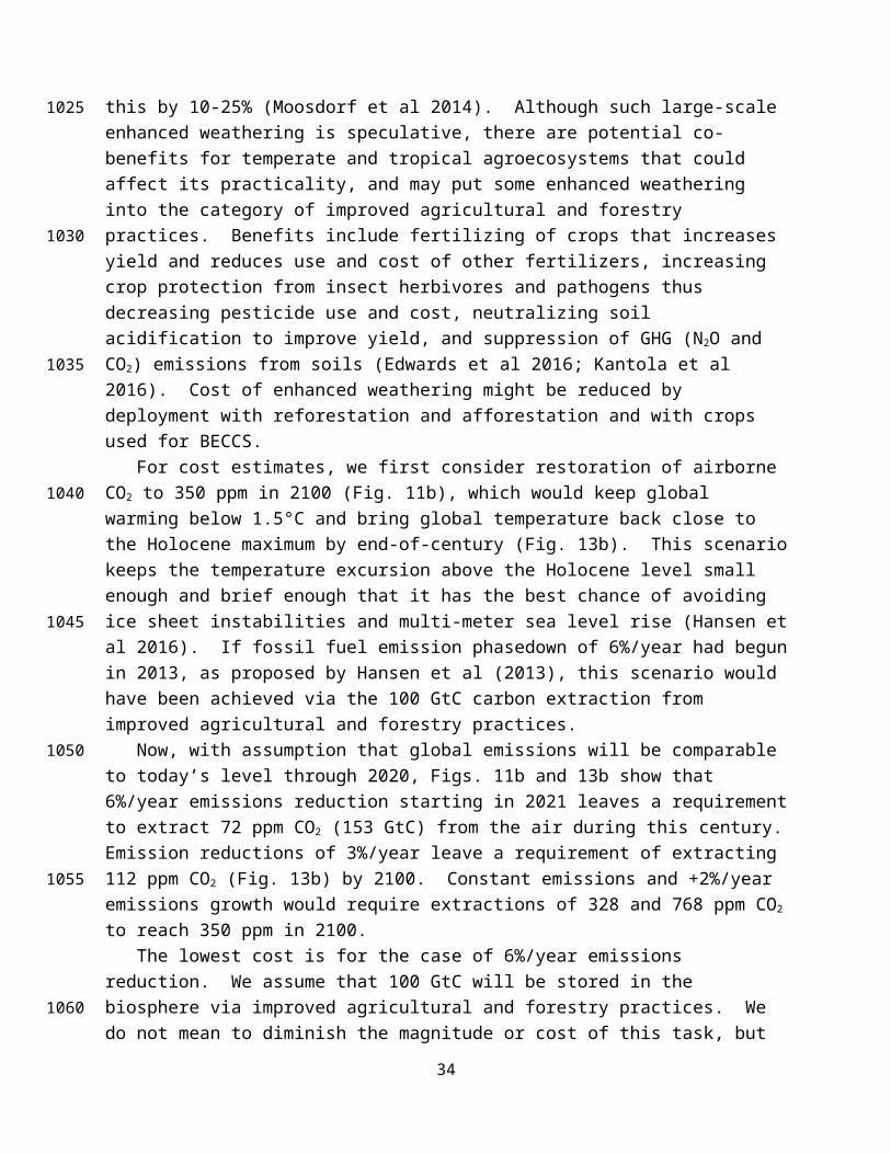
Fuss, S., Canadell, J. G., Peters, G. P., Tavoni, M., Andrew, R. M., Ciais, P., Jackson, R. B., Jones, C. D., Kraxner, F., Nakicenovic, N., Le Quere, C., Raupach, M. R., Sharifi, A., Smith, P., and Yamagata, Y.: Betting on negative emissions, Nature Clim Change, 4, 850-853, 2014.

Fyfe, J. C., Meehl, G. A., England, M. H., Mann, M. E., Santer, B. D., Flato, G. M., Hawkins, E., Gillett, N. P., Xie, S., Kosaka, Y., and Swart, N. C.: Making sense of the early-2000s warming slowdown, Nature Clim Change, 6, 224-228, 2016.

Grant, K. M., Rohling, E. J., Bar-Matthews, M., Ayalon, A., Medina-Elizalde, M., Ramsey, C. B., Satow, C., and Roberts, A. P.: Rapid coupling between ice volume and polar temperature over the past 150,000 years, Nature, 491, 744-747, 2012.

Grant, K. M., Rohling, E. J., Bronk, Ramsey. C., Cheng, H., Edwards, R. L., Florindo, F., Heslop, D., Marra, F., Roberts, A. P., Tamisiea, M. E., and Williams, F.: Sea-level variability over five glacial cycles, Nature Comm, 5, 5076, doi:10.1038/ncomms6076, 2014.

Hansen, J., Sato, M., Ruedy, R., Lacis, A., and Oinas, V.: Global warming in the twenty-first century: An alternative scenario, Proc Natl Acad Sci USA, 97, 9875-9880, 2000.

Hansen, J. and Sato, M.: Greenhouse gas growth rates, Proc Natl Acad Sci USA, 101, 16109-16114, 2004.

Hansen, J., Sato, M., Ruedy, R., Nazarenko, L., Lacis, A., Schmidt, G. A., Russell, G., Aleinov, I., Bauer, M., Bauer, S., Bell, N., Cairns, B., Canuto, V., Chandler, M., Cheng, Y., Del Genio, A., Faluvegi, G., Fleming, E., Friend, A., Hall, T., Jackman, C., Kelley, M., Kiang, N. Y., Koch, D., Lean, J., Lerner, J., Lo, K., Menon, S., Miller, R. L., Minnis, P., Novakov, T., Oinas, V., Perlwitz., J.P., Perlwitz, J., Rind, D., Romanou, A., Shindell, D., Stone, P., Sun, S., Tausnev, N., Thresher, D., Wielicki, B., Wong, T., Yao, M., and Zhang, S.: Efficacy of climate forcings, J Geophys Res, 110, D18104, doi:10.1029/2005JD005776, 2005.

Hansen, J.: Climate threat to the planet: implications for energy policy and intergenerational justice, Bjerknes lecture, American Geophysical Union, San Francisco, 17 December, available at: http://www.columbia.edu/~jeh1/2008/AGUBjerknes20081217. pdf (last access: 10 August 2016), 2008

Hansen, J., Sato, M., Kharecha, P., Beerling, D., Berner, R., Masson-Delmotte, V., Pagani, M., Raymo, M., Royer, D. L., and Zachos, J. C.: Target atmospheric CO2: Where should humanity aim? Open Atmos Sci J, 2, 217-231, 2008.

Hansen, J., Ruedy, R., Sato, M., and Lo, K.: Global surface temperature change , Rev Geophys, 48, RG4004, 2010.

Hansen, J., Sato, M., Kharecha, P., and von Schuckmann, K.: Earth's energy imbalance and implications , Atmos Chem Phys, 11, 13421-13449, doi:10.5194/acp-11-13421-2011, 2011.

Hansen, J., Kharecha, P., Sato, M., Masson-Delmotte, V., Ackerman, F., Beerling, D. J., Hearty, P. J., Hoegh-Guldberg, O., Hsu, S., Parmesan, C., Rockstrom, J., Rohling, E. J., Sachs, J., Smith, P., Steffen, K., Van Susteren, L. von Schuckmann, K., and Zachos, J. C.: Assessing "dangerous climate change": Required reduction of carbon emissions to protect young people, future generations and nature , Plos One, 8, e81648, 2013.

Hansen, J. E.: Environment and development challenges: the imperative of a carbon fee and dividend The Oxford Handbook of the Macroeconomics of Global Warming editors Bernard L and Semmler W DOI:10.1093/oxfordhb/9780199856978,013.0026Oxford University Press, 2014.

Hansen, J. and Sato, M.: Regional climate change and national responsibilities, Environ Res Lett, 11, published online 2 March, doi:10.1088/1748-9326/11/3/034009, 2016.

Hansen, J., Sato, M., Hearty, P., Ruedy, R., Kelley, M., Masson-Delmotte, V., Russell, G., Tselioudis, G., Cao, J., Rignot, E., Velicogna, I., Tormey, B., Donovan, B., Kandiano, E., von Schuckmann, K., Kharecha, P., Legrande, A. N., Bauer, M., and Lo, K.-W.: Ice melt, sea level rise and superstorms: Evidence from paleoclimate data, climate modeling, and modern observations that 2°C global warming could be dangerous, Atmos. Chem. Phys., 16, 3761-3812, 2016.

34

1150

1155

1160

1165

1170

1175

1180

1185

Hartmann, D.L., Klein Tank, A. M. G., Rusticucci, M., Alexander, L. V., Brönnimann, S., Charabi, Y., Dentener, F. J., Dlugokencky, E. J., Easterling, D. R., Kaplan, A., Soden, B. J., Thorne, P. W., Wild, M. and Zhai, P. M.: Observations: Atmosphere and Surface. In: Climate Change 2013: The Physical Science Basis, edited by: Stocker, T.F., Qin, D., Plattner, G.-K., Tignor, M., Allen, S. K., Boschung, J., Nauels, A., Xia, Y., Bex, V., and Midgley, P. M., Cambridge University Press, Cambridge, United Kingdom, 2013.

Hedenus, F., Wirsenius, S., and Johansson, D. J. A.: The importance of reduced meat and dairy consumption for meeting stringent climate change targets, Clim Change, 124, 79, doi:10.1007/s10584-014-1104-5, 2014.

Holmes, C. D., Prather, M. J., Sovde, O. A., and Myhre, G.: Future methane, hydroxyl, and their uncertainties: key climate and emission parameters for future predictions, Atmos Chem Phys, 13, 285-302, 2013.

Hope, M.: Temperature spiral goes viral, Nature Clim Change, 6, 657, 2016.

Howarth, R. W.: Methane emissions and climatic warming risk from hydraulic fracturing and shale gas development: implications for policy, Energy Emission Control Tech, 3, 45-54, 2015.

Hsu, S. L.: The Case for a Carbon Tax, Island Press, Washington D.C., p 233, 2011.

Huang, B., Banzon, V. F., Freeman, E., Lawrimore, J., Liu, W., Peterson, T. C., Smith, T. M., Thorne, P. W., Woodruff, S. D., and Zhang, H.-M.: Extended reconstructed sea surface temperature Version 4 (ERSST.v4). Part I: Upgrades and intercomparisons, J Clim, 28, 911-930, 2015.

Huntingford, C., Lowe, J. A., Gohar, L. K., Bowerman, N. H., Allen, M. R., Raper, S. C., and Smith, S. M.: The link between a global 2°C warming threshold and emissions in years 2020, 2050 and beyond, Environ Res Lett, 7, 014039, 2012.

IPCC (Intergovernmental Panel on Climate Change): Special Report on Emissions Scenarios, edited by: Nakicenovic, N. and Swart, R., Cambridge University Press, ISBN 0-521-80081-1, 978-052180081-5 (pb: 0-521-80493-0, 978-052180493-6), 2000.

IPCC (Intergovernmental Panel on Climate Change): IPCC Guidelines for National Greenhouse Gas Inventories Volume 4 Agriculture, Forestry and Other Land Use, edited by: Eggleston, H. S., Buendia, L., Miwa, K., Ngara, T., and Tanabe, K., IGES Japan http://www.ipcc-nggip.iges.or.jp/, 2006.

IPCC (Intergovernmental Panel on Climate Change): Climate Change 2013, edited by: Stocker, T., Qin, D., Q., Plattner, G. K., Tignor, M. M. B., Allen, S. K., Boschung, J., Nauels, A., Xia, Y., Bex, V., and Midgley, P. M., Cambridge University Press, 1535 pp., 2013.

IPCC (Intergovernmental Panel on Climate Change): Climate Change 2014: Impacts, Adaptation, and Vulnerability, Field, C., Barros, V. R., Dokken, D. J., Mach, K. J., and Mastrandrea, M. D., Cambridge University Press, 1132 pp., 2014.

Jackson, R. B., Canadell, J. G., Le Quere, C., Andrew, R. M., Korsbakken, J. I., Peters, G. P., and Nakicenovic, N.: Reaching peak emissions, Nature Clim Change, 6, 7-10. 2016.

Jones, C.D., Ciais, P., Davis, S.J., Friedlingstein, Gasser, T., Peter, G.P., Rogelj, J., van Vuuren, D. P., Canadell, J. G., Cowie, A., Jackson, R. B., Jonas, M., Kriegler, E., Littleton, E., Lowe, J. A., Milne, J., Shrestha, G., Smith, P., Torvanger, A., and Wiltshire, A.: Simulating the Earth system response to negative emissions, Environ Res Lett, (ERL-102404.R1 - accepted), 2016.

Joos, F., Bruno, M., Fink, R., Stocker, T. F., Siegenthaler, U., Le, Quere. C., and Sarmiento, J. L.: An efficient and accurate representation of complex oceanic and biospheric models of anthropogenic carbon uptake, Tellus, 48B, 397-417, 1996.

Judd, A. G., Hovland, M., Dimitrov, L. I., Garcia, Gil. S., and Jukes, V.: The geological methane budget at Continental Margins and its influence on climate change, Geofluids, 2, 109-126, 2002.

35

1190

1195

1200

1205

1210

1215

1220

1225

1230

Juliana et al vs United States: Kelsey Cascadia Rose Juliana et al v The United States of America; Barack Obama, in his official capacity as President of the United States; et al United States District Court, District of Oregon, Eugene Division Case no.: 6:15-cv-01517-TC, hearing held on 13 September 2016 on defendant's motion to dismiss case, decision pending, 2016.

Kantola, I. B., McMasters, M. D., Beerling, D. J., Long, S. P., and DeLucia, E. H.: Potential of global croplands and bioenergy crops for climate change mitigation through deployment for enhanced weathering, (submitted) http://mc.manuscriptcentral.com/bl, 2016.

Keeling, C, D., Whorf, T. P., Wahlen, M., and van der Plicht, J.: Interannual extremes in the rate of rise of atmospheric carbon dioxide since 1980, Nature, 375, 666-670, 1973.

Keith, D. W., Ha-Duong, M., and Stolaroff, J. K.: Climate strategy with CO2 capture from the air, Clim Change, 74, 17-45, 2006.

Keith, D.: Why capture CO2 from the atmosphere, Science, 325, 1654-1655, 2009.

Kharecha, P. A. and Hansen, J. E.: Implications of “peak oil” for atmospheric CO2 and climate, Global Biogeochemical Cycles, 22, GB3012 doi:10.1029/2007GB003142, 2008.

Kohler, P., Hartman, J., and Wolf-Gladrow, D. A.: Geoengineering potential of artificially enhanced silicate weathering of olivine, Proc Natl Acad Sci USA, 107, 20228-20233, 2010.

Kopp, G., Krivova, N., Lean, J., and Wu, C. J.: The Impact of the Revised Sunspot Record on Solar Irradiance Reconstructions , Solar Physics, doi:10.1007/s11207-016-0853-x, 2016.

Kosaka, Y. and Xie, S. P.: Recent global-warming hiatus tied to equatorial Pacific surface cooling, Nature, 501, 403-407, 2013.

Kroeze, C. and Bouwman, L.: The role of nitrogen in climate change, Curr Opin Environ Sustain, 3, 279-280, 2011.

Kvenvolden, K. A.: Gas hydrates – Geological perspective and global change, Rev Geophys, 31, 173-187, 1993.

Kyoto Protocol: available at: http://unfccc.int/kyoto_protocol/items/2830.php (last access: 9 September 2016 ), 1997.

Levitus, S., Antonov, J. I., Boyer, T. P., Baranova, O. K., Garcia, H. E., Locarnini, R. A., Mishonov, A. V., Regan, J. R., Seidov, D., Yarosh, E. S., and Zweng, M. M.: World ocean heat content and thermosteric sea level change (0-2000 m), 1955-2010, Geophys Res Lett, 39, L10603 doi:10.1029/2012GL051106, 2012.

Liu, X. and Zhang, F.: Nitrogen fertilizer induced greenhouse gas emissions in China, Curr Opin Environ Sustain, 3, 407-413, 2011.

Liu, Z., Zhu, J., Rosenthal, Y., Zhang, X., Otto-Bliesner, B. L., Timmermann, A., Smith, R. S., Lohmann, G., Zheng, W., and Timm, O. E.: The Holocene temperature conundrum, Proc Natl Acad Sci USA, published online 11 August, doi:10.1073/pnas.1407229111, 2014.

Marcott, S. A., Shakun, J. D., Clark, P. U., and Mix, A. C.: A reconstruction of regional and global temperature for the last 11,300, Science, 339, 1198-1201, 2013.

Marcott, S. A. and Shakun, J. D.: Holocene climate change and its context for the future, PAGES News, 23 (1), 28, 2015.

Masson-Delmotte, V., Schulz, M., Abe-Ouchi, A., Beer, J., Ganopolski, A., Gonzalez Rouco, J. F., Jansen, E., Lambeck, K., Luterbacher, J., Naish, T., Osboorn, T., Otto-Bliesner, B., Quinn, T., Ramexh, R., Rojas, M. Shao, X., and Timmermann, A.: Information from paleoclimate Archives, in: Climate Change 2013: The Physical Basis, edited by: Stocker, T. F., Qin, D., Plattner, G.-K., Tignor, M., Allen, S. K., Boschung, J., Nauels, A., Xia, Y., Bex, V., and Midgley, P. M., Cambridge University Press, Cambridge, United Kingdom, 2013.

36

1235

1240

1245

1250

1255

1260

1265

1270

McKay, N. P., Overpeck, J. T., and Otto-Bliesner, B. L.: The role of ocean thermal expansion in Last Interglacial sea level rise, Geophys Res Lett, 38, L14605, doi:10.1029/2011GL048280, 2011.

Meehl, G. A., Teng, H., and Arblaster, J. M.: Climate model simulations of the observed early-2000s hiatus of global warming, Nature Clim Change, published online 7, September doi:10.1038/nclimate2357, 2014.

Meinshausen, M., Wigley, T. M. L., and Raper, S. C. B.: Emulating atmosphere-ocean and carbon cycle models with a simpler model, MAGICC6 – Part 2: Applications, Atmos Chem Phys, 11, 1457-1471, 2011.

Menne, M. J., Durre, I., Vose, R. S., Gleason, B. E. and Houston, T. G.: An overview of the Global Historical Climatology Network-Daily database, J. Atmos. Ocean Technol, 29, 897-910, 2012.

Montreal Protocol 2016: The Montreal Protocol on Substances that Deplete the Ozone Layer, available at: http://www.ozone.unep.org/ (last access: 19 June 2016), 2016.

Montzka, S. A., Krol, M., Dlugokencky, E., Hall, B., Jockel, P., and Lelieveld, J.: Small interannual variability of global atmospheric hycroxyl, Science, 331, 67-69, 2011.

Moosdorf, N., Renforth, P., and Hartmann, J.: Carbon dioxide efficiency of terrestrial enhanced weathering, Environ Sci Tech, 48, 4809-4816, 2014.

Moss, R. H., Edmonds, J. A., Hibbard, K. A., Manning, M. R., Rose, S. K., van Vuuren, D. P., Carter, T. R., Emori, S., Kainuma, M., Kram, T., Meehl, G. A., Mitchell, J. F. B., Nakicenovic, N., Riahi, K., Smith, S. J., Stouffer, R. J., Thomson, A. M., Weyant, J. P., and Wilbanks, T. J.: The next generation of scenarios for climate change research and assessment, Nature, 463, 747-756, 2010.

Myhre, G., Shindell, D., Breon, F., Collins, W., Fuglestvedt, J., Huang, J., Koch, D., Lamarque, J. F., Lee, D., Mendoza, B., Nakajima, T., Robock, A., Stephens, G., Takemura, T., and Zhang, H: Anthropogenic and natural climate forcing, in: Climate Change 2013: The Physical Basis, edited by: Stocker, T. F., Qin, D., Plattner, G.-K., Tignor, M., Allen, S. K., Boschung, J., Nauels, A., Xia, Y., Bex, V., and Midgley, P. M., Cambridge University Press, Cambridge, United Kingdom, 2013.

National Academy of Sciences (NAS): Attribution of Extreme Weather Events in the Context of Climate Change, National Academies Press, doi:10.17226/21852, 2016.

Newman, P. A., Oman, L.D., Douglass, A. R., Fleming, E. L., Frith, S. M., Hurwitz, M. M., Kawa, S. R., Jackman, C. H., Krotkov, N. A., Nash, E. R., Nielsen, J. E., Pawson, S., Stolarski, R. S., and Velders, G. J. M.: What would have happened to the ozone layer if chlorofluorocarbons (CFCs) had not been regulated? Atmos Chem Phys, 9, 2113-2128, 2009.

Novakov, T., Ramanathan, V., Hansen, J. E., Kirchstetter, T. W., Sato, M., Sinton, J. E., and Sathaye, J. A.: Large historical changes of fossil-fuel black carbon aerosols, Geophys Res Lett, 30, 1324, doi:10.1029/2005JD005977, 2003.

NRC (National Research Council): Climate Intervention: Carbon Dioxide Removal and Reliable Sequestration, The National Academies Press Washington DC, 154 pp, doi:10.17226/18805, available at: www.nap.edu/catalog/18805/climate-intervention-carbon-dioxide-removal-and-reliable-sequestration, 2015.

O’Connor, F. M., Boucher, O., Gedney, N., Jones, C. D., Folberth, G. A., Coppell, R., Friedlingstein, P., Collins, W. J., Chappellaz, J., Ridley, J., and Johnson, C. E.: Possible role of wetlands, permafrost, and methane hydrates in the methane cycle under future climate change: A review, Rev Geophys, 48, RG4005 doi:10.1029/2010RG000326, 2010.

Paris Agreement 2015, UNFCCC secretariat, available at "Paris Agreement, FCCC/CP/2015/L.9/Rev.1" (PDF), 12 December 2015 (last access: 9 September 2016), 2015.

Park, S., Croteau, P., Boering, K. A., Etheridge, D. M., Ferretti, D., Fraser, P. J., Kim, K. R., Krummel, P. B., Langenfelds, R. L., van Ommen, T. D., Steele, L. P., and Trudinger. C. M.: Trends and seasonal cycles in the isotopic composition of nitrous oxide sine 1940, Nature Geosci, 5, 261-265, 2012.

37

1275

1280

1285

1290

1295

1300

1305

1310

1315

Peters, G. P., Andrew, R. M., Boden, T., Canadell, J. G., Ciais, P., Le Quéré, C., Marland, G., Raupach, M. R., and Wilson, C.: The challenge to keep global warming below 2°C, Nature Clim Change, 3, 4-6, 2013.

Peterson, T. C. and Vose, R.: An overview of the global historical climatology network temperature database, Bull Amer Meteorol Soc, 78, 2837-2849, 1997.

Pollard, D., DeConto, R. M., and Alley, R. B.: Potential Antarctic ice sheet retreat driven by hydrofracturing and ice cliff failure, Earth Planet Sci Lett, 412, 112-121, 2015.

Popp, A., Lotze-Campen, H., and Bodirsky, B.: Food consumption, diet shifts and associated non-CO2 greenhouse gases, Global Environ Change, 20, 451-462, 2010.

Prather, M., Midgley, P., Rowland, F. S., and Stolarski, R.: The ozone layer: the road not taken, Science, 381, 551-554, 1996.

Prather, M. J., Holmes, C. D., and Hsu, J.: Reactive greenhouse gas scenarios: systematic exploration of uncertainties and the role of atmospheric chemistry, Geophys Res Lett, 39, L09803, 2012.

Prather, M. J., Hsu, J., Deluca, N. M., Jackman, C. H., Oman, L. D., Douglass, A. R., Fleming, E. L., Strahan, S. E., Steenrod, S. D., Sovde, O. A., Isaksen, I. S. A., Froidevaux, L., and Funke, B.: Measuring and modeling the lifetime of nitrous oxide including its variability, J Geophys Res Atmos, 120, 5693-5705, 2015.

Purkey, S.G. and Johnson, G.S.: Antarctic bottom water warming and freshening: contributions to sea level rise, ocean freshwater budgets, and global heat gain, J. Climate, 26, 6105-6122, 2013.

Rajaratnam, B., Romano, J., Tsiang, M., and Diffenbaugh, N. S.: Debunking the climate hiatus, Clim Change, 133, 129-140, 2015.

Reeburgh, W. S.: Oceanic methane biogeochemistry, Chem Rev, 107, 486-513, 2007.

Rhein, M., Rintoul, S. R., Aoki, S., Campos, E., Chamber, D., Feely, R. A., Gulev, S., Johnson, G. C., Josey, S. A., Kostianoy, A., Mauritzen, C. Roemmich, D., Talley, L. D., and Wang, F.: Observations: Ocean, in: Climate Change 2013: The Physical Basis, Contribution of Working Group I to the Fifth Assessment Report of the Intergovernmental Panel on Climate Change, edited by: Stocker, T. F., Qin, D., Plattner, G.-K., Tignor, M., Allen, S. K., Boschung, J., Nauels, A., Xia, Y., Bex, V., and Midgley, P. M., Cambridge University Press, Cambridge, United Kingdom, 2013.

Rignot, E., Jacobs, S., Mouginot, J., and Scheuchl, B.: Ice shelf melting around Antarctica, Science, 341, 266-270, 2013.

Rockmann, T. and Levin, I.: High-precision determination of the changing isoptopic composition of atmospheric N2O from 1990 to 2002, J Geophys Res Atmos, 110, D21304, 2005.

Rogelj, J., Meinshausen, M., and Knutti, R.: Global warming under old and new scenarios using IPCC climate sensitivity range estimates, Nature Clim Change, 2, 248-253, 2012.

Rogelj, J., den Elzen, M., Hohne, N., Franzen, T., Fekete, H., Winkler, H., Schaeffer, R., Sha, F., Rihi, K., and Meinshausen, M.: Paris Agreement climate proposals need a boost to keep warming well below 2°C Probabilistic cost estimates for climate change mitigation, Nature, 534, 631-639, 2016a.

Rogelj, J., Schaeffer, M., Friedlingstein, P., Gillett, N. P., van Vuuren, D. P., Riahi, K., Allen, M., and Knutti, R.: Differences between carbon budget estimates unraveled, Nature Clim Change, 534, 631-639, 2016b.

Rohling, E. J., Sluijs, A., Dijkstra, H., Köhler, P., van de Wal, R.S., von der Heydt, A., Beerling, D., Berger, A., Bijl, P., Crucifix, M., DeConto, R., Drijfhout, S., Fedorov, A., Foster, G., Ganopolski, A., Hansen, J., Hönisch, B., Hooghiemstra, H., Huber, M., Huybers, P., Knutti, R., Lea, D., Lourens, L.J., Lunt, D., Masson-Delmotte, V., Medina-Elizalde, M., Otto-Bliesner, B., Pagani, M., Pälike, H., Renssen, H., Royer, D., Siddall, M., Valdes, P.,

38

1320

1325

1330

1335

1340

1345

1350

1355

Zachos, J.C., Zeebe, R.E.: Making sense of palaeoclimate sensitivity, Nature, 491, 683-691, doi:10.1038/nature11574, 2012a.

Rohling, E. J., Medina-Elizade, M., Shepherd, J. G., Siddall, M., and Stanford, J. D.: Sea surface and high-latitude temperature sensitivity to radiative forcing of climate over several glacial cycles, J Clim, 25, 1635-1656, 2012b.

Rohling, E. J., Haigh, I. D., Foster, G. L., Roberts, A. P., and Grant, K. M.: A geological perspective on potential future sea-level rise, Scientific Reports, 3, 3461 doi:10.1038/srep03461, 2013.

Sanderson, B. M., O’Neill, B. C., and Tebaldi, C.: What would it take to achieve the Paris temperature targets? Geophys Res Lett, 43, doi:10.1002/2016GL069563, 2016.

Sato, M., Hansen, J. E., McCormick, M. P., and Pollack, J. B.: Stratospheric aerosol optical depths, 1850-1990, J Geophys Res, 98, 22987-22994, doi:10.1029/93JD02553, 1993.

Schädel, C., Bader, M. K.-F., Schuur, E. A. G., Biasi, C., Bracho, R., Čapek, P., De Baets, S., Diáková, K., Ernakovich, J., Estop-Aragones, C., Graham, D. E., Hartley, I. P., Iversen, C. M., Kane, E., Knoblauch, C., Lupascu, M., Martikainen, P. J., Natali, S. M., Norby, R. J., O’Donnell, J. A., Chowdhury, T. R., Šantrůčková, H., Shaver, G., Sloan, V. L., Treat, C. C., Turetsky, M. R., Waldrop, M. P., and Wickland, K. P.: Potential carbon emissions dominated by carbon dioxide from thawed permafrost soils, Nature Clim Change, doi:10.1038/nclimate3054, 2016.

Schaefer, H., Mikaloff Fletcher, S. E., Veidt, C., Lassey, K. R., Brailsford, G. W., Bromley, T. M., Dlugokencky, E. J., Michel, S. E., Miller, J. B., Levin, I., Lowe, D. C., Martin, R. J., Vaughn, B. H., White, J. W. C.: A 21st century shift from fossil-fuel to biogenic methane emissions indicated by 13CH4, Science, 352, 80-84, 2016.

Schmittner, A., Urban, N.M., Shakun, J.D., Mahowald, N.M., Clark, P.U., Bartlein, P.J., Mix, A.C. and Rosell-Mele, A.: Climate sensitivity estimated from temperature reconstructions of the Last Glacial Maximum, Science, 334, 1385-1388, 2011.

Schuur, E. A. G., McGuire, A. D., Schadel, C., Grosse, G., Harden, J. W., Hayes, D. J., Hugelius, G., Koven, C. D., Kuhry, P., Lawrence, D. M., Natali, S. M., Olefeldt, D., Romanovsky, V. E., Schaefer, K., Turetsky, M. R., Treat, C. C., and Vonk, J. E.: Climate change and the permafrost carbon feedback, Nature, 520, 171-179, 2015.

Schwalm, C. R., Williams, C. A., Schaefer, K., Baker, I., Collatz, G. J., and Rödenbeck, C.: Does terrestrial drought explain global CO2 flux anomalies induced by El Nino?, Biogeosci, 8, 2493-2506, 2011.

Seidel, D. J., Fu, Q., Randel, W. J., and Reichler, T. J.: Widening of the tropical belt in a changing climate, Nature Geosci, 1, 21-24, 2008.

Smith, P.: Soil carbon sequestration and biochar as negative emission technologies, Global Change Biology, 22, 1315-1324, 2016.

Smith, P., Davis, S. J., Creutzig, F., Fuss, S., Minx, J., Gavrielle, B., Kato, E., Jackson, R. B., Cowie, A., Kriegler, E., van Vuuren, D. P., Rogelj, J., Ciais, P., Milne, J., Canadell, J. G., McCollum, D., Peters, G., Andrew, R., Krey, V., Shrestha, G., Friedlingstein, P., Gasser, T., Grübler , A., Heidug, W. K., Jonas, M., Jones, C. D., Kraxner, F., Littleton, E., Lowe, J., Moreira, J. R., Nakicenovic, N., Obersteiner, M., Patwardhan, A., Rogner, M., Rubin, E., Sharifi, A., Torvanger, Asbjørn, Yamagata, Y., Edmonds, J., and Yongsung, C.: Biophysical and economic limits to negative CO2 emissions, Nature Clim Change, 6, 42-50, 2016.

Smith, T. M., Reynolds, R. W., and Lawrimore, J.: Improvements to NOAA’s historical merged land-ocean surface temperature analysis (1880-2006), J Clim, 21, 2283-2296, 2008.

Socolow, R.: Direct air capture of CO2 with chemicals: a technology assessment for the APS Panel on Public Affairs (American Physical Society), 2011.

SIPRI (Stockholm International Peace Research Institute): SIPRI Military Expenditure Database, available at: https://www.sipri.org/databases/milex, (last access: 17 September 2016), 2016.

39

1360

1365

1370

1375

1380

1385

1390

1395

Taylor, L. L., Quirk, J., Thorley, R. M. S., Kharecha, P. A., Hansen, J., Ridgwell, A., Lomas, M. R., Banwart, S. A., and Beerling, D. J.: Enhanced weathering strategies for stabilizing climate and averting ocean acidification, Nature Clim Change, 6, 402-406, 2016.

Thompson, D. W. J., Kennedy, J. J., Wallace, J. M., and Jones, P. D.: A large discontinuity in the mid-twentieth century in observed global-mean surface temperature, Nature, 453, 646-649 doi:10.1038/nature06982, 2008.

Tilman, D. and Clark, M.: Global diets link environmental sustainability and human health, Nature, 515, 518-522, 2014.

Trenberth, K. E. and Fasullo, J. T.: An apparent hiatus in global warming?, Earth’s Future, doi:10.1002/2013EF000165, 2013.

Trenberth, K., Fasullo, J., von Schuckmann, K., and Cheng, L.: Insights into Earth’s energy imbalance from multiple sources, J Clim, doi:10.1175/JCLI-D-16-0339.1 in press, 2016.

Turner, A. J., Jacob, D. J., Benmergui, J., Wofsy, S. C., Maasakkers, J. D., Butz, A., Hasekamp, O., and Biraud, S. C.: A large increase in U.S. methane emissions over the past decade inferred from satellite data and surface observations, Geophys Res Lett, 43, 2218–2224, doi:10.1002/2016GL067987, 2016.

Turney, C. S. M. and Jones, R. T.: Does the Agulhas Current amplify global temperatures during super-interglacials?, J Quatern Sci, 25, 839-843, 2010.

Tyndall, J.: On the absorption and radiation of heat by gases and vapours, and on the physical connexion of radiation, absorption, and conduction – The Bakerian Lecture, Phil Mag, 22, 273-285, 1861.

United Nations: Framework Convention on Climate Change (UNFCCC), United Nations, New York, NY, available at: http: //unfccc.int/essential_background/items/6036.php (last access: 3 March 2016), 1992.

van Vuuren, D. P., Edmonds, J., Kainuma, M., Riahi, K., Thomson, A., Hibbard, K., Hurtt, G. C., Kram, T., Krey, V., Lamarque, J.-F., Masui, T., Meinshausen, M., Nakicenovic, N., Smith, S. J., and Rose, S. K.: The representative concentration pathways: an overview, Clim Change, 109, 5-31, 2011.

Vial, J., Dufresne, J. L., and Bony, S.: On the interpretation of inter-model spread in CMIP5 climate sensitivity estimates, Clim Dyn, published online 23 March, doi:10.1007/s00382-013-1725-9, 2013.

von Schuckmann, K. and Le Traon, P. Y.: How well can we derive Global Ocean Indicators from Argo data?, Ocean Sci, 7, 783-791 doi:10.5194/os-7-783-2011, 2011.

von Schuckmann, K., Palmer, M. D., Trenberth, K. E., Cazenave, A., Chamber, D., Champollion, N., Hansen, J., Josey, S. A., Loeb, N., Mathieu, P. P., Meyssignac, B., and Wild, M.: An imperative to monitor Earth’s energy imbalance, Nature Clim Change, 6, 138-144, 2016.

Voulgarakis, A., Naik, V., Lamarque, J.-F., Shindell, D. T., Young, P. J., Prather, M. J., Wild, O., Field, R. D., Bergmann, D., Cameron-Smith, P., Cionni, I., Collins, W. J., Dalsøren, S. B., Doherty, R. M., Eyring, V., Faluvegi, G., Folberth, G. A., Horowitz, L. W., Josse, B., MacKenzie, I. A., Nagashima, T., Plummer, D. A., Righi, M., Rumbold, S. T., Stevenson, D. S., Strode, S. A., Sudo, K., Szopa, S., and Zeng, G.: Analysis of present day and future OH and methane lifetime in the ACCMIP simulations, Atmos Chem Phys, 13, 2503-2587, 2013.

Williamson, P.: Scrutinize CO2 removal methods, Nature, 530, 153-155, 2016.

Woolf, D., Amonette, J. E., Street-Perrott, F. A., Lehmann, J., and Joseph, S.: Sustainable biochar to mitigate global climate change, Nature Comm, 1, 56 doi:10.1038/ncomms1053, 2010.

40

1400

1405

1410

1415

1420

1425

1430

1435