· The research conducted by the U.S. Army Engineer Research and Development Center (ERDC) included review and evaluation of the Sheppard-Melville and the Federal Highway Administrat

ERD

C TR

-16-

10

Application of Bridge Pier Scour Equations for Large Woody Vegetation

Engi

neer

Res

earc

h an

d D

evel

opm

ent

Cent

er

Deborah R. Cooper, Charles D. Little, Jr., Julie Cohen, Brendan Yuill, Johannes Wibowo, Bryant Robbins, Raymond Reed, Maureen K. Corcoran, and Kevin S. Holden

July 2016

Approved for public release; distribution is unlimited.

The U.S. Army Engineer Research and Development Center (ERDC) solves the nation’s toughest engineering and environmental challenges. ERDC develops innovative solutions in civil and military engineering, geospatial sciences, water resources, and environmental sciences for the Army, the Department of Defense, civilian agencies, and our nation’s public good. Find out more at www.erdc.usace.army.mil.

To search for other technical reports published by ERDC, visit the ERDC online library at http://acwc.sdp.sirsi.net/client/default.

http://www.erdc.usace.army.mil/

http://acwc.sdp.sirsi.net/client/default

ERDC TR-16-10 July 2016


Brendan T. Yuill, Johannes Wibowo, Bryant Robbins, and Maureen K. Corcoran Geotechnical and Structures Laboratory U.S. Army Engineer Research and Development Center 3909 Halls Ferry Road Vicksburg, MS 39180-6199

Deborah Cooper, Charles D. Little, Jr., Julie Cohen, and Raymond Reed Coastal and Hydraulics Laboratory U.S. Army Engineer Research and Development Center 3909 Halls Ferry Road Vicksburg, MS 39180-6199

Kevin S. Holden Institute for Water Resources, Risk Management Center 12596 West Bayaud Avenue, Suite 400 Lakewood, CO 80228

Final report Approved for public release; distribution is unlimited.

Prepared for U.S. Army Corps of Engineers Washington, DC 20314-1000

Monitored by Project Number 454633

ERDC TR-16-10 ii

Abstract

Existing bridge pier scour prediction equations exclude the influence of tree roots and the cross slope of levee embankments. Developed for specific conditions, these equations do not include modeling of scour at trees near or on levee embankments. Therefore, existing bridge pier scour models must be carefully evaluated and possibly modified before being applied to tree scour.

The research conducted by the U.S. Army Engineer Research and Development Center (ERDC) included review and evaluation of the Sheppard-Melville and the Federal Highway Administration Hydraulic Engineering Circular No. 18 (FHWA HEC-18) bridge pier scour equations and validation flume experiments. The research objective was to provide guidance for predicting maximum scour depths near trees on or near levee embankments. The Sheppard-Melville and the HEC-18 methods of bridge pier scour prediction were evaluated. Results from the flume experiments indicate that both methods consistently over-predict scour depth by as much as 25 to 75 percent. Although other bridge scour equations can be used, both the Sheppard-Melville and the HEC-18 equations are sufficient in assessing tree scour potential to conservatively estimate maximum scour that may occur.

DISCLAIMER: The contents of this report are not to be used for advertising, publication, or promotional purposes. Citation of trade names does not constitute an official endorsement or approval of the use of such commercial products. All product names and trademarks cited are the property of their respective owners. The findings of this report are not to be construed as an official Department of the Army position unless so designated by other authorized documents. DESTROY THIS REPORT WHEN NO LONGER NEEDED. DO NOT RETURN IT TO THE ORIGINATOR.

ERDC TR-16-10 iii

Contents Abstract .......................................................................................................................................................... ii

Figures and Tables ........................................................................................................................................ iv

Preface ........................................................................................................................................................... ix

Unit Conversion Factors ...............................................................................................................................x

1 Introduction ............................................................................................................................................ 1

2 Background ............................................................................................................................................ 3

3 Bridge Pier Scour Models .................................................................................................................... 5 3.1 Sheppard-Melville method ............................................................................................ 5 3.2 FHWA HEC-18 method................................................................................................... 7

4 Flume Experiments ............................................................................................................................... 8 4.1 Small flume experiments .............................................................................................. 8 4.2 Large flume experiments ............................................................................................ 11

5 Experimental Results ......................................................................................................................... 14 5.1 Small flume results...................................................................................................... 14

5.1.1 Results for small flume tests with full obstruction (h/y=1) .................................... 14 5.1.2 Results for small flume tests with partial obstructions (h/y<1) ............................. 14 5.1.3 Results of small flume tests with engineered root ball pit ..................................... 20

5.2 Large flume results ...................................................................................................... 21 5.2.1 Results of large flume tests with full obstructions (h/y=1) .................................... 22 5.2.2 Results of large flume tests with partial obstructions (h/y<1) ............................... 24 5.2.3 Results of large flume tests with tree/root ball ....................................................... 25

6 Discussion of Applicability to Large Woody Vegetation Scour .................................................. 28 6.1 Application to the standing tree case ......................................................................... 28 6.2 Application to fallen tree/root ball case ..................................................................... 29

7 Summary and Recommendations ................................................................................................... 31

References ................................................................................................................................................... 33

Appendix A: Small Flume Experiments .................................................................................................. 34

Appendix B: Large Flume Experiments .................................................................................................. 66

Report Documentation Page

ERDC TR-16-10 iv

Figures and Tables

Figures

Figure 1. Example of small flume test configuration for square pier shape. ......................................... 9 Figure 2. Example of large flume test configuration: cylinder diameter of 0.92 m and gravel test bed. ............................................................................................................................................. 11 Figure 3. Standing tree test configuration, pretest. ................................................................................. 12 Figure 4. Fallen tree test configuration, pretest. ...................................................................................... 13 Figure 5. Comparison of observed and predicted normalized scour depth ys/a* for Sheppard-Melville method, small flume tests with full obstruction (h/y=1). ....................................... 16 Figure 6. Comparison of observed and predicted normalized scour depth ys/a* for HEC-18 method, small flume tests with full obstruction (h/y=1). ....................................................................... 17 Figure 7. Comparison of observed and predicted normalized scour depth ys/a* for Sheppard-Melville method, small flume tests with partial obstruction (h/y<1). ................................. 18 Figure 8. Comparison of observed and predicted normalized scour depth ys/a* for HEC-18 method, small flume tests with partial obstruction (h/y<1). ................................................................. 19 Figure 9. Correction coefficient for partial-obstruction scour depths. .................................................. 20 Figure 10. Comparison of observed and predicted normalized scour depths for Sheppard-Melville method, small and large flume tests. ......................................................................................... 23 Figure 11. Comparison of observed and predicted normalized scour depths for HEC-18 method, small and large flume tests. ........................................................................................................ 23 Figure 12. Comparison of partial obstruction correction factors for small and large flume tests. ............................................................................................................................................................... 24 Figure 13. Comparison of observed and predicted normalized scour depths for Sheppard-Melville method, small and large flume tests with tree/root ball. ......................................................... 26 Figure 14. Comparison of observed and predicted normalized scour depths for HEC-18 method, small and large flume tests with tree/root ball. ....................................................................... 27 Figure A-1. Original model configuration. .................................................................................................. 36 Figure A-2. Cylindrical and square obstructions. ..................................................................................... 37 Figure A-3. Model sand gradation. ............................................................................................................. 38 Figure A-4. Nixon 402 digital flowmeter. ................................................................................................... 39 Figure A-5. Handheld laser scanner and scanning apparatus. ............................................................. 40 Figure A-6. Laser scanner reference plane. ............................................................................................. 40 Figure A-7a. Photograph image of scour. .................................................................................................. 41 Figure A-8. Test 1. Scour upstream of 3.18-cm cylindrical obstruction, full flow depth obstruction, Q=0.04 m3/s, Vavg=27.43 cm/s, flow depth = 15.24 cm, t = 3 hr. .................................. 44 Figure A-9. Test 2. Scour upstream of 4.76-cm cylindrical obstruction, full flow depth obstruction, Q=0.04 m3/s, Vavg=27.43 cm/s, flow depth = 15.24 cm, t = 3 hr. .................................. 44 Figure A-10. Test 3. Scour upstream of 3.18-cm cylindrical obstruction, full flow depth obstruction, Q=0.02 m3/s, Vavg=21.31 cm/s, flow depth = 7.62 cm, t = 3 hr. .................................... 45 Figure A-11. Test 4. Scour upstream of 4.76-cm cylindrical obstruction, full flow depth obstruction, Q=0.02 m3/s, Vavg=21.31 cm/s, flow depth = 7.62 cm, t = 3 hr. .................................... 45

ERDC TR-16-10 v

Figure A-12. Test 5. Scour upstream of 3.18-cm cylindrical obstruction, obstruction submerged 7.62 cm (50 percent flow depth obstruction), Q=0.04 m3/s, Vavg=27.43 cm/s, flow depth = 15.24 cm, t = 3 hr. ................................................................................................................ 46 Figure A-13. Test 6. Scour upstream of 4.76-cm cylindrical obstruction, obstruction submerged 7.62 cm (50 percent flow depth obstruction), Q=0.04 m3/s, Vavg=27.43 cm/s, flow depth = 15.24 cm, t = 3 hr. ................................................................................................................ 46 Figure A-14. Test 27. Scour upstream of 3.18-cm cylindrical obstruction, obstruction submerged 3.81 cm (75 percent flow depth obstruction), Q=0.04 m3/s, Vavg=27.43 cm/s, flow depth = 15.24 cm, t = 3 hr. ................................................................................................................ 47 Figure A-15. Test 28. Scour upstream of 4.76-cm cylindrical obstruction, obstruction submerged 3.81 cm (75 percent flow depth obstruction), Q=0.04 m3/s, Vavg=27.43 cm/s, flow depth = 15.24 cm, t = 3 hr. ................................................................................................................ 47 Figure A-16. Test 29. Scour upstream of 3.18-cm cylindrical obstruction obstruction submerged 11.43 cm (25 percent flow depth obstruction), Q=0.04 m3/s, Vavg=27.43 cm/s, flow depth = 15.24 cm, t = 3 hr. ................................................................................. 48 Figure A-17. Test 30. Scour upstream of 4.76-cm cylindrical obstruction, obstruction submerged 11.43 cm (25 percent flow depth obstruction), Q=0.04 m3/s, Vavg=27.43 cm/s, flow depth = 15.24 cm, t = 3 hr. ................................................................................. 49 Figure A-18. Model with square obstructions. ......................................................................................... 50 Figure A-19a. Test 7. Scour upstream of 2.54-cm-square obstruction, obstruction submerged 7.62 cm (50 percent flow depth obstruction), t = 0 hr. ...................................................... 51 Figure A-20a. Test 8. Scour upstream of 5.01-cm-square obstruction, obstruction submerged 7.62 cm (50 percent flow depth obstruction), t = 0 hr. ...................................................... 52 Figure A-21. Square obstructions with preformed scour holes. ............................................................ 53 Figure A-22a. Test 9. Scour upstream of 2.54-cm-square obstruction, obstruction submerged 7.62 cm (50 percent flow depth obstruction), 2.54-cm x 2.54-cm x 1.27-cm preformed scour, t = 0 hr............................................................................................................................. 54 Figure A-23a. Test 10. Scour upstream of 5.08-cm-square obstruction, obstruction submerged 7.62 cm (50 percent flow depth obstruction), 5.08-cm x 5.08-cm x 1.27-cm preformed scour, t = 0 hr............................................................................................................................. 55 Figure A-24b. Q=0.04 m3/s, Vavg=27.43 cm/s, flow depth = 15.24 cm, t = 3 hr. ............................... 55 Figure A-25. Test 11. Scour upstream of 2.54-cm-square obstruction, obstruction submerged 7.62 cm (50 percent flow depth obstruction), 2.54-cm x 2.54-cm x 0.84-cm preformed scour, Q=0.04 m3/s, Vavg=27.43 cm/s, flow depth = 15.24 cm, t = 3 hr. ........................ 56 Figure A-26. Test 12. Scour upstream of 5.08-cm-square obstruction, obstruction submerged 7.62 cm (50 percent flow depth obstruction), 5.08-cm x 5.08-cm x 1.68-cm preformed scour, Q=0.04 m3/s, Vavg=27.43 cm/s, flow depth = 15.24 cm, t = 3 hr. ........................ 56 Figure A-27a. Test 13. Scour upstream of 2.54-cm-square obstruction, obstruction submerged 7.62 cm (50 percent flow depth obstruction), 1.27-cm x 2.54-cm x 0.84-cm preformed scour, t = 0 hr............................................................................................................................. 57 Figure A-28a. Test 14. Scour upstream of 5.08-cm-square obstruction, obstruction submerged 7.62 cm (50 percent flow depth obstruction), 2.54-cm x 5.08-cm x 1.68-cm preformed scour, t = 0 hr............................................................................................................................. 58 Figure A-29. Test 15. Scour upstream of 2.54-cm-square obstruction, obstruction submerged 7.62 cm (50 percent flow depth obstruction), 2.54-cm x 2.54-cm x 0.84-cm preformed scour, Q=0.04 m3/s, Vavg=27.43 cm/s, flow depth = 15.24 cm, t= 3 hr. ....................... 59

ERDC TR-16-10 vi

Figure A-30. Test 16. Scour upstream of 5.08-cm-square obstruction, obstruction submerged 7.62 cm (50 percent flow depth obstruction), 5.08-cm x 5.08-cm x 1.68-cm preformed scour, Q=0.04 m3/s, Vavg=27.43 cm/s, flow depth = 15.24 cm, t = 3 hr. ........................ 59 Figure A-31. Test 17. Scour upstream of 2.54-cm-square obstruction, obstruction submerged 11.43 cm (25 percent flow depth obstruction), Q=0.04 m3/s, Vavg=27.43 cm/s, flow depth = 15.24 cm, t = 3 hr. ............................................................................... 60 Figure A-32. Test 18. Scour upstream of 5.08-cm-square obstruction, obstruction submerged 11.43 cm (25 percent flow depth obstruction), Q=0.04 m3/s, Vavg=27.43 cm/s, flow depth = 15.24 cm, t = 3 hr. ............................................................................... 60 Figure A-33. Test 19. Scour upstream of 2.54-cm-square obstruction, obstruction submerged 11.43 cm (25 percent flow depth obstruction), Q=0.04 m3/s, Vavg=27.43 cm/s, flow depth = 15.24 cm, t = 3 hr. ............................................................................... 61 Figure A-34. Test 20. Scour upstream of 5.08-cm-square obstruction, obstruction submerged 11.43 cm (25 percent flow depth obstruction), Q=0.04 m3/s, Vavg=27.43 cm/s, flow depth = 15.24 cm, t = 3 hr. ............................................................................... 61 Figure A-35. Test 23. Scour upstream of 2.54-cm-square obstruction, obstruction submerged 3.81 cm (75 percent flow depth obstruction), Q=0.04 m3/s, Vavg=27.43 cm/s, flow depth = 15.24 cm, t = 3 hr. ................................................................................................................ 62 Figure A-36. Test 24. Scour upstream of 5.08-cm-square obstruction, obstruction submerged 3.81 cm (75 percent flow depth obstruction), Q=0.04 m3/s, Vavg=27.43 cm/s, flow depth = 15.24 cm, t = 3 hr. ................................................................................................................ 62 Figure A-37. Test 25. Scour upstream of 2.54-cm-square obstructions, 100 percent flow depth obstruction, Q=0.04 m3/s, Vavg = 27.43 cm/s, flow depth = 15.24 cm, t = 3 hr. .................... 63 Figure A-38. Test 26. Scour upstream of 5.08-cm-square obstruction, 100 percent flow depth obstruction, Q=0.04 m3/s, Vavg = 27.43 cm/s, flow depth = 15.24 cm, t = 3 hr. .................... 63 Figure B-1. Phase I gravel bed model layout. ........................................................................................... 67 Figure B-2. Gravel bed gradation. .............................................................................................................. 68 Figure B-3. Phase II sand bed model layout. ............................................................................................ 70 Figure B-4. Sand bed gradation for Phase II testing. ............................................................................... 71 Figure B-5. Phase III model layout.............................................................................................................. 72 Figure B-6. Marsh-McBirney Flo-Mate 2000 portable flow meter©. .................................................... 74 Figure B-7. Vectrino adv velocimeter©. ..................................................................................................... 74 Figure B-8. Pretest photograph of 0.92-m-diam cylinder. ....................................................................... 76 Figure B-9. Pretest photogrammetry point cloud of 0.92-m-diam cylinder. ......................................... 76 Figure B-10. Test 1B point cloud created using photogrammetry software, 0.51-m-diam cylinder in gravel, fully obstructed flow, Vavg = 0.76 m/s, d = 0.7 m, t = 7.5 hr. ................................... 78 Figure B-11. Analysis of Test 1B using Crater Pro© Software 0.51-m-diam cylinder in gravel, fully obstructed flow, Vavg = 0.76 m/s, d = 0.7 m, t = 7.5 hr. ...................................................... 79 Figure B-12. Test 2B point cloud created using photogrammetry software, 0.92-m-diam cylinder in gravel, fully obstructed flow, Vavg = 0.76 m/s, d = 0.7 m, t = 7.5 hr. ................................... 80 Figure B-13. Analysis of Test 2B using Crater Pro© Software 0.92-m-diam cylinder in gravel, fully obstructed flow, Vavg = 0.76 m/s, d = 0.7 m, t = 7.5 hr. ...................................................... 81 Figure B-14. Test 3B point cloud created using photogrammetry software, 0.51-m-diam cylinder in gravel, submerged flow, Vavg = 0.76 m/s, d = 0.7 m, t = 7.5 hr. .......................................... 82 Figure B-15. Analysis of Test 3B using Crater Pro© Software, 0.51-m-diam cylinder in gravel, submerged flow, Vavg = 0.76 m/s, d = 0.7 m, t = 7.5 hr. ............................................................. 83

ERDC TR-16-10 vii

Figure B-16. Test 4B point cloud created using photogrammetry software 0.92-m-diam cylinder in gravel, submerged flow, Vavg = 0.76 m/s, d = 0.7 m, t = 7.5 hr. .......................................... 84 Figure B-17. Analysis of Test 4B using Crater Pro© Software, 0.92-m-diam cylinder in gravel, submerged flow, Vavg = 0.76 m/s, d = 0.7 m, t = 7.5 hr.............................................................. 85 Figure B-18. Test 5B point cloud created using photogrammetry software, 0.92-m-diam cylinder in sand, submerged flow, Vavg = 0.35 m/s, d = 0.7 m, t = 7.5 hr. ........................................... 87 Figure B-19. Analysis of Test 5B using Crater Pro© software,0.92-m-diam cylinder in sand, submerged flow, Vavg = 0.35 m/s, d = 0.7 m, t = 7.5 hr. ......................................................................... 88 Figure B-20. Test 6B point cloud created using photogrammetry software, 0.92-m-diam cylinder in sand, fully obstructed flow, Vavg = 0.35 m/s, d = 0.7 m, t = 7.5 hr...................................... 89 Figure B-21. Analysis of Test 6B using Crater Pro© software, 0.92-diam cylinder in sand, fully obstructed flow, Vavg = 0.35 m/s, d = 0.7 m, t = 7.5 hr. .................................................................. 90 Figure B-22. Test 7B point cloud created using photogrammetry software, tree in fallen position in sand, tree floating, Vavg = 0.35 m/s, d = 0.7 m, t = 7.5 hr. .................................................. 92 Figure B-23. Analysis of Test 7B using Crater Pro© software, tree in fallen position in sand, tree floating, Vavg = 0.35 m/s, d = 0.7 m, t = 7.5 hr. ..................................................................... 93 Figure B-24. Test 8B point cloud created using photogrammetry software, tree in fallen position in sand, tree stationary, Vavg = 0.35 m/s, d = 0.7 m, t = 7.5 hr. .............................................. 94 Figure B-25. Analysis of Test 8B using Crater Pro© software, tree in fallen position in sand, tree stationary, Vavg = 0.35 m/s, d = 0.7 m, t = 7.5 hr. ................................................................. 95 Figure B-26. Standing tree in flume on blue barrel. ................................................................................ 96 Figure B-27. Test 9B, tree in vertical position in sand, fully obstructed flow, Vavg = 0.35 m/s, d = 0.7 m, t = 3 hr. ............................................................................................................................. 96 Figure B-28. Test 9B point cloud created using photogrammetry software, tree in vertical position in sand, fully obstructed flow, Vavg = 0.35 m/s, d = 0.7 m, t = 3 hr. ....................................... 97 Figure B-29. Analysis of Test 9B using Crater Pro© software, tree in vertical position in sand, fully obstructed flow, Vavg = 0.35 m/s, d = 0.7 m, t = 3 hr. ........................................................ 98 Figure B-30. Test 10B point cloud created using photogrammetry software, tree in vertical position in sand, fully obstructed flow, Vavg = 0.35 m/s, d = 0.7 m, t = 7.5 hr. .................................... 99 Figure B-31. Analysis of Test 10B using Crater Pro© software, tree in vertical position in sand, fully obstructed flow, Vavg = 0.35 m/s, d = 0.7 m, t = 7.5 hr. ................................................. 100

Tables

Table 1. Small flume experiment configurations. .................................................................................... 10 Table 2. Large flume experiment configurations. .................................................................................... 13 Table 3. Experimental results for complete small flume test matrix. .................................................... 15 Table 4. Summary of results for small flume tests with full obstruction (h/y=1). ............................... 16 Table 5. Summary of small flume tests with partial obstruction (h/y<1). ............................................ 17 Table 6. Summary of small flume tests with preformed root ball pit. ................................................... 21 Table 7. Experimental results for complete large flume test matrix. ..................................................... 22 Table A-1. Small flume scour test matrix for cylindrical obstructions. .................................................. 42 Table A-2. Small flume scour test matrix: Q= 0.04 m3s, Vavg=27.43 cm/s, depth = 15.24 cm. ...................................................................................................................................................... 43 Table A-3. Small flume scour depths, cylindrical obstructions, t = 3 hr. ............................................... 43

ERDC TR-16-10 viii

Table A-4. Small flume scour depths, square obstructions, Q=0.04 m3/s, Vavg=27.43 cm/s, depth = 15.24 cm, t = 3 hr. ......................................................................................... 64 Table B-1. Scour study experimental testing matrix. ............................................................................... 77

ERDC TR-16-10 ix

Preface

This study was conducted for the Headquarters, U.S. Army Corps of Engineers (HQUSACE). The Technical Monitor was Dr. Michael K. Sharp of the Office of Technical Directors (GZT).

The work was performed by the River Engineering Branch of the Flood and Storm Protection Division, U.S. Army Engineer Research and Development Center Coastal and Hydraulics Laboratory (CHL) and the Geotechnical Engineering and Geosciences Branch (GEGB) of the Geosciences and Structures Division (GSD) in the Geotechnical and Structures Laboratory (GSL), with support from the Institute for Water Resources (IWR), Risk Management Center (RMC). At the time of publication, Dr. James Lewis was Acting Chief, CEERD-HFRS; Ty Wamsley was Chief, CEERD-HF; Chad A. Gartrell was Chief, CEERD-GSG; Dr. Amy Bednar was Acting Chief, CEERD-GSD; and Dr. Michael K. Sharp, CEERD-GZT, was the Technical Director for Water Resources Infrastructure. The Deputy Director of ERDC-CHL was Dr. Kevin Barry, and the Director was Jose Sanchez. The Deputy Director of GSL was Dr. William P. Grogan. The Director of GSL was Bartley P. Durst. The Director of RMC was Nathan J. Snorteland, and the Director of IWR was Robert A. Pietrowsky.

COL Bryan S. Green was the Commander of ERDC, and Dr. Jeffery P. Holland was the Director.

ERDC TR-16-10 x

Unit Conversion Factors

Multiply By To Obtain

cubic feet 0.02831685 cubic meters

cubic feet per second 0.02831685 cubic meters per second

cubic inches 1.6387064 E-05 cubic meters

cubic yards 0.7645549 cubic meters

feet 0.3048 meters

feet per second 0.3048 meters per second

inches 25.4 millimeters

square feet 0.09290304 square meters

square inches 6.4516 E-04 square meters

yards 0.9144 meters

ERDC TR-16-10 1

1 Introduction

Scour has been studied extensively over the last 50 years for quantifying the erosion of river bed sediment around submerged bridge abutments and piers. Through these studies, numerous empirical equations have been developed to predict the magnitude of local scour at a bridge site. Because of the structural similarity between bridge piers and large woody vegetation, such as trees, these equations have also been employed to predict erosion due to vegetation in and around river channels. However, there have been few studies assessing the performance of bridge scour equations to model tree scour. Further, evaluation of these equations over the years has revealed that they typically over-predict the actual observed scour (Ettema et al. 2011; Yuill, in preparation).

In addition to being conservative, existing bridge pier scour prediction equations include variables that are not pertinent to scour in the vicinity of large woody vegetation. Many important factors are excluded, such as tree root influence and, in the case of vegetation near levees, the cross slope of levee embankments. This is not a shortcoming of existing models but rather an observation that these models were developed for specific conditions that do not include modeling of scour at trees near or on levee embankments. Therefore, existing bridge pier scour models must be carefully evaluated and possibly modified before being applied to tree scour.

The results of this research provide general guidelines for assessing scour associated with large woody vegetation that can be readily used in evaluating the impact of predicted scour on levee performance, safety, and integrity. This report documents the results of flume experiments used to validate the use of bridge scour equations in assessing tree scour.

Flume validation experiments included both small flume (0.91 m wide by 0.3 m deep) and large flume (7.32 m wide by 3.05 m deep) tests conducted for clear-water scour conditions. The small flume tests were conducted to (1) verify the prediction trends of two selected bridge pier scour models, the Sheppard-Melville equation (Sheppard et al. 2011) and the Federal Highway Administration Hydraulic Circular No. 18 (FHWA HEC-18) method, also known as the Colorado State University (CSU) equation (Richardson and Davis 2001), and (2) to investigate potential model

ERDC TR-16-10 2

corrections/modifications for scour associated with submerged root balls/ stumps. The large flume experiments were conducted to validate modifications/corrections of the scour predictor models developed in the small flume experiments and to investigate scour associated with an actual tree/root ball. The objective of these flume validation experiments was to develop methods and guidance for application of existing bridge pier scour equations to the case of tree scour.

ERDC TR-16-10 3

2 Background

The discussion is divided into two categories: (1) small woody vegetation, such as shrubbery, brush, or woody groundcovers, and (2) large woody vegetation (i.e., trees). In the case of small woody vegetation, there is potential for the vegetation to increase resistance to scour. The velocity of the water, coupled with the lack of rigidity of the vegetation, typically results in the vegetation being bent over with the flow, forming an erosion-resistant mat on the ground. The increased roughness from this mat significantly reduces near-bed velocities and, thus, reduces boundary shear stress, the primary driver of sediment erosion. Even if this vegetation should become uprooted, the smaller root system of the plants typically does not form a significant root pit that could potentially develop into an enlarged scour hole. The research reported herein does not address the case of small woody vegetation.

In the case of standing large woody vegetation, the stems are usually sufficiently rigid to resist bending under the flow. In this case, tree trunks may affect flow patterns and potential scour in a manner similar to that observed at bridge piers. Increased turbulence due to vortices formed in the accelerated flow field around the tree trunk may result in increased scour in the vicinity of the tree. However, the subsurface root structure of the tree may provide some measure of scour resistance. These potential effects of standing trees are largely unknown, as little significant research has been conducted in this area.

Another problematic situation is presented by the case of overturned large trees with exposed root pits. Dependent on soil properties and the tree species, the exposed root pit can be significant in both depth and diameter. Water flow through the root pit will be extremely turbulent, such that normal stresses due to the vertically accelerated flow, may be as or more critical than the boundary shear stresses in terms of erosion potential. The enlargement of the root pit due to turbulence-induced scour may potentially result in the compromise of the critical levee section required for levee safety. In addition, the root ball has potential to cause scour by redirecting the flow toward the bed or causing additional turbulence. Again, no significant research has been conducted to develop prediction methods for scour associated with fallen trees.

ERDC TR-16-10 4

The U.S. Army Corps of Engineers (USACE) guidance for variance from current policy requirements pertaining to vegetation control on and near flood-control levees requires applicants to demonstrate that excepted vegetation will not adversely affect levee performance. The potential effects of vegetation on scour are typically investigated using existing bridge pier scour models. The lack of proven efficacy in the application of bridge pier scour models to vegetation scour scenarios limits the variance process in terms of both applicant analysis and agency review. The research reported herein improves applicability of bridge pier scour models to vegetation scour prediction. However, further research is needed to improve the knowledge base on scour associated with large woody vegetation.

ERDC TR-16-10 5

3 Bridge Pier Scour Models

A comprehensive review and evaluation of existing bridge pier scour models was conducted and reported by Yuill (in preparation). The models were evaluated in regard to their potential use in assessing scour associated with standing or fallen large woody vegetation. The most significant parameters of each model in terms of applicability to vegetation scour were identified and reported. A comprehensive list of scour models was evaluated, but only the Sheppard-Melville equation and the FHWA HEC-18 equation were selected for validation with the flume experiments reported herein. These two equations were selected because they are either currently recommended for use in the FHWA manual or have recently been suggested as an alternative equation for the manual (Ettema et al. 2011).

3.1 Sheppard-Melville method

The Sheppard-Melville method (Sheppard et al. 2011) was developed from the scour prediction equation proposed by Sheppard and Miller (2006) and follows a similar parameter approach reported by Melville (1997). The method is presented in the National Cooperative Highway Research Program (NCHRP) Project 24-27 (01) report (Ettema et al. 2011). Only the clear-water scour (i.e., scour when reach-scale bed material transport is minimal, 0.4< average approach velocity (V)/ sediment critical velocity (Vc) <1) portion of the method was used in this research, as clear-water scour conditions produce maximum scour depths while representing conservative conditions. For clear-water scour conditions,

*

* *.s

c

y y V af f fa a V D

1 2 3

50

2 5 (1)

where

.

* *

y yf tanha a

0 4

1

.c c

V Vf lnV V

2

2 1 1 2

ERDC TR-16-10 6

*

*

. .* *

. .

aDaf

D a aD D

503 1 2 0 13

50

50 50

0 4 10 6

and

ys = equilibrium scour depth y = approach flow depth a* = effective pier width D50 = bed material diameter where 50 percent are finer.

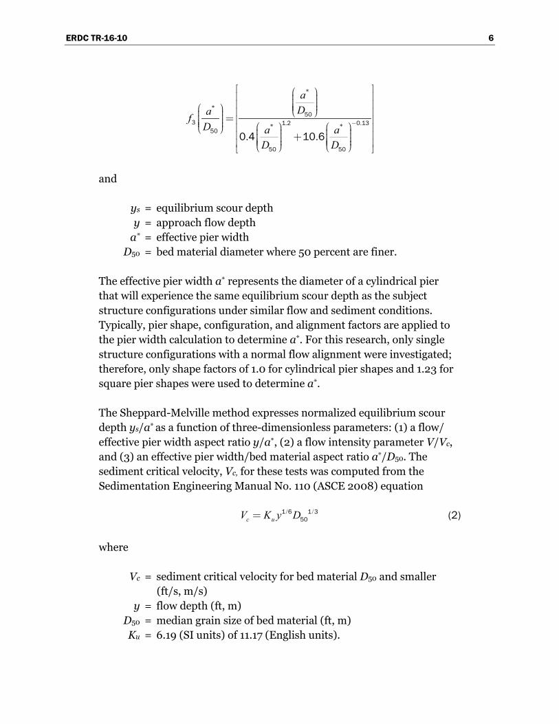
The effective pier width a* represents the diameter of a cylindrical pier that will experience the same equilibrium scour depth as the subject structure configurations under similar flow and sediment conditions. Typically, pier shape, configuration, and alignment factors are applied to the pier width calculation to determine a*. For this research, only single structure configurations with a normal flow alignment were investigated; therefore, only shape factors of 1.0 for cylindrical pier shapes and 1.23 for square pier shapes were used to determine a*.

The Sheppard-Melville method expresses normalized equilibrium scour depth ys/a* as a function of three-dimensionless parameters: (1) a flow/effective pier width aspect ratio y/a*, (2) a flow intensity parameter V/Vc, and (3) an effective pier width/bed material aspect ratio a*/D50. The sediment critical velocity, Vc, for these tests was computed from the Sedimentation Engineering Manual No. 110 (ASCE 2008) equation

/ /c uV K y D 1 6 1 3

50 (2)

where

Vc = sediment critical velocity for bed material D50 and smaller (ft/s, m/s)

y = flow depth (ft, m) D50 = median grain size of bed material (ft, m) Ku = 6.19 (SI units) of 11.17 (English units).

ERDC TR-16-10 7

3.2 FHWA HEC-18 method

The FHWA uses a bridge pier scour method by Richardson and Davis (2001) in the HEC-18 guidance manual. Often referred to as the Colorado State University (CSU) equation due to of the location of its development, the method extends back more than 35 years and has undergone several updates (Richardson and Davis 1995, 2001). The method is based on the equation

.

..sw

y yK K K K K Fra a

0 350 43

1 2 3 42 0 (3)

where

ys = equilibrium scour depth (ft, m) y = approach flow depth (ft, m) a = pier width (ft, m) Fr = Froude Number, 𝑉𝑉

√𝑔𝑔𝑔𝑔

K1 = correction factor for pier shape K2 = correction factor for flow angle K3 = correction factor for bed sediment condition K4 = correction factor for armoring Kw = correction factor for wide piers (HEC-18 version only).

Similar to the Sheppard-Melville method, the HEC-18 method expresses normalized equilibrium scour depth as a function of flow-depth/pier-width aspect ratio and Froude number for flow intensity. For this research, the only correction factor that was required was K1 for pier shape, with values of 1.0 for cylindrical shapes and 1.1 for square shapes.

ERDC TR-16-10 8

4 Flume Experiments

Detailed descriptions of the experimental procedures and results for the small flume and large flume tests are provided in Appendices A and B, respectively. These appendices present the detailed test apparatus setups, the experimental controls, test data collection, and post-processing.

4.1 Small flume experiments

The small flume experiments for clear-water scour conditions were designed to (1) determine the accuracy of the Sheppard-Melville method and the HEC-18 method of scour depth prediction and to (2) determine the effects of submerged obstacles on predicted scour depths. In terms of the first purpose, the small flume experiment results give a general indication of whether the scour prediction methods tend to over-predict or under-predict scour depths. Foundational assumptions in planning the small flume tests are that standing trees can essentially be treated as bridge piers in terms of scour prediction for vegetation assessment purposes and that predicted scour can be considered a conservative maximum due to potential erosion resistance from the root structure of the tree, which may be significant but is not included in this analysis. Treating a standing tree as a bridge pier also assumes that the tree will act as an obstacle to flow throughout the entire water depth. This may not be the case, however, with a fallen tree having an exposed root ball, as addressed in the second purpose. In this situation, the root ball will act as a much wider pier than the tree trunk (assuming perpendicular orientation of the root ball to the direction of flow) and may not obstruct the entire vertical profile of the flow. It is probable that the entire root ball would be submerged during major flood events that inundate the floodplain by several feet. The effect of submerged obstacles on pier scour depths has not been well-studied and documented; therefore, a series of small flume tests with varying submerged pier conditions was conducted to determine correction factors to use with the bridge pier equations in the case of submerged obstacles. The case of fallen trees also includes the presence of exposed root ball pits. Additional small flume tests were developed to include engineered root ball pits at the base of the submerged obstacles. However, the noncohesive nature of the small flume bed material made it difficult for the engineered pit to remain intact during the initiation of the tests before steady flow conditions were achieved.

ERDC TR-16-10 9

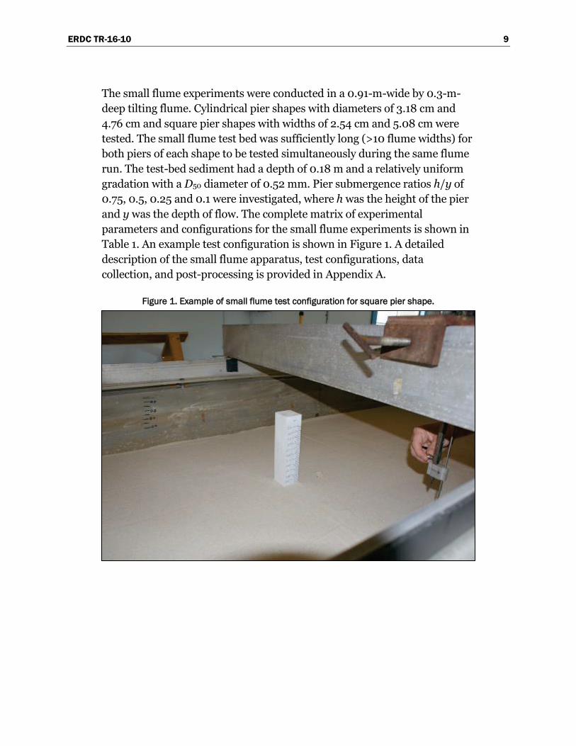
The small flume experiments were conducted in a 0.91-m-wide by 0.3-m-deep tilting flume. Cylindrical pier shapes with diameters of 3.18 cm and 4.76 cm and square pier shapes with widths of 2.54 cm and 5.08 cm were tested. The small flume test bed was sufficiently long (>10 flume widths) for both piers of each shape to be tested simultaneously during the same flume run. The test-bed sediment had a depth of 0.18 m and a relatively uniform gradation with a D50 diameter of 0.52 mm. Pier submergence ratios h/y of 0.75, 0.5, 0.25 and 0.1 were investigated, where h was the height of the pier and y was the depth of flow. The complete matrix of experimental parameters and configurations for the small flume experiments is shown in Table 1. An example test configuration is shown in Figure 1. A detailed description of the small flume apparatus, test configurations, data collection, and post-processing is provided in Appendix A.

Figure 1. Example of small flume test configuration for square pier shape.

ERDC TR-16-10 10

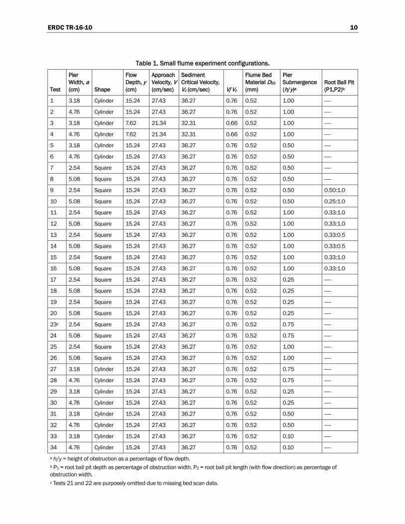
Table 1. Small flume experiment configurations.

Test

Pier Width, a (cm) Shape

Flow Depth, y (cm)

Approach Velocity, V (cm/sec)

Sediment Critical Velocity, Vc (cm/sec) V/Vc

Flume Bed Material D50 (mm)

Pier Submergence (h/y)a

Root Ball Pit (P1,P2)b

1 3.18 Cylinder 15.24 27.43 36.27 0.76 0.52 1.00 -----

2 4.76 Cylinder 15.24 27.43 36.27 0.76 0.52 1.00 -----

3 3.18 Cylinder 7.62 21.34 32.31 0.66 0.52 1.00 -----

4 4.76 Cylinder 7.62 21.34 32.31 0.66 0.52 1.00 -----

5 3.18 Cylinder 15.24 27.43 36.27 0.76 0.52 0.50 -----

6 4.76 Cylinder 15.24 27.43 36.27 0.76 0.52 0.50 -----

7 2.54 Square 15.24 27.43 36.27 0.76 0.52 0.50 -----

8 5.08 Square 15.24 27.43 36.27 0.76 0.52 0.50 -----

9 2.54 Square 15.24 27.43 36.27 0.76 0.52 0.50 0.50:1.0

10 5.08 Square 15.24 27.43 36.27 0.76 0.52 0.50 0.25:1.0

11 2.54 Square 15.24 27.43 36.27 0.76 0.52 1.00 0.33:1.0

12 5.08 Square 15.24 27.43 36.27 0.76 0.52 1.00 0.33:1.0

13 2.54 Square 15.24 27.43 36.27 0.76 0.52 1.00 0.33:0.5

14 5.08 Square 15.24 27.43 36.27 0.76 0.52 1.00 0.33:0.5

15 2.54 Square 15.24 27.43 36.27 0.76 0.52 1.00 0.33:1.0

16 5.08 Square 15.24 27.43 36.27 0.76 0.52 1.00 0.33:1.0

17 2.54 Square 15.24 27.43 36.27 0.76 0.52 0.25 -----

18 5.08 Square 15.24 27.43 36.27 0.76 0.52 0.25 -----

19 2.54 Square 15.24 27.43 36.27 0.76 0.52 0.25 -----

20 5.08 Square 15.24 27.43 36.27 0.76 0.52 0.25 -----

23c 2.54 Square 15.24 27.43 36.27 0.76 0.52 0.75 -----

24 5.08 Square 15.24 27.43 36.27 0.76 0.52 0.75 -----

25 2.54 Square 15.24 27.43 36.27 0.76 0.52 1.00 -----

26 5.08 Square 15.24 27.43 36.27 0.76 0.52 1.00 -----

27 3.18 Cylinder 15.24 27.43 36.27 0.76 0.52 0.75 -----

28 4.76 Cylinder 15.24 27.43 36.27 0.76 0.52 0.75 -----

29 3.18 Cylinder 15.24 27.43 36.27 0.76 0.52 0.25 -----

30 4.76 Cylinder 15.24 27.43 36.27 0.76 0.52 0.25 -----

31 3.18 Cylinder 15.24 27.43 36.27 0.76 0.52 0.50 -----

32 4.76 Cylinder 15.24 27.43 36.27 0.76 0.52 0.50 -----

33 3.18 Cylinder 15.24 27.43 36.27 0.76 0.52 0.10 -----

34 4.76 Cylinder 15.24 27.43 36.27 0.76 0.52 0.10 -----

a h/y = height of obstruction as a percentage of flow depth. b P1 = root ball pit depth as percentage of obstruction width. P2 = root ball pit length (with flow direction) as percentage of obstruction width. c Tests 21 and 22 are purposely omitted due to missing bed scan data.

ERDC TR-16-10 11

4.2 Large flume experiments

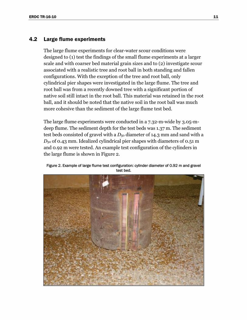
The large flume experiments for clear-water scour conditions were designed to (1) test the findings of the small flume experiments at a larger scale and with coarser bed material grain sizes and to (2) investigate scour associated with a realistic tree and root ball in both standing and fallen configurations. With the exception of the tree and root ball, only cylindrical pier shapes were investigated in the large flume. The tree and root ball was from a recently downed tree with a significant portion of native soil still intact in the root ball. This material was retained in the root ball, and it should be noted that the native soil in the root ball was much more cohesive than the sediment of the large flume test bed.

The large flume experiments were conducted in a 7.32-m-wide by 3.05-m-deep flume. The sediment depth for the test beds was 1.37 m. The sediment test beds consisted of gravel with a D50 diameter of 14.3 mm and sand with a D50 of 0.43 mm. Idealized cylindrical pier shapes with diameters of 0.51 m and 0.92 m were tested. An example test configuration of the cylinders in the large flume is shown in Figure 2.

Figure 2. Example of large flume test configuration: cylinder diameter of 0.92 m and gravel test bed.

ERDC TR-16-10 12

The trunk of the tree for the standing tree tests tapered from an approximate diameter of 0.67 m at the test-bed surface to an approximate diameter of 0.27 m at the water surface as shown in Figure 3. A weighted “effective” diameter of 0.41 m was computed by dividing the total area obstructed by the trunk by the total water depth (obstructed depth). The fallen tree root ball configuration resulted in an obstruction width of 0.96 m as shown in Figure 4. The purpose of the test was to model the root ball obstruction as a pier of equal width as the rootball. The effect of the tree trunk size in relation to the root ball was not addressed. The root ball size is less than what could occur in the field, but it was the most practical for test application in the flume. Although flow around the tree trunk may affect the size and shape of the scour hole, it does not significantly affect the depth. The fallen tree with root ball test configuration resulted in a full depth obstruction, and no submerged root ball tests were conducted. Note that the width of the root ball obstruction is nearly identical to the diameter of the largest cylinder.

The complete test matrix for the large flume experiment parameters is shown in Table 2. The V/Vc ratio for the tests with the gravel bed was lower than that for the other tests due to pump limitations for the given flow depth. A detailed description of the large flume apparatus, test configura-tions, data collection, and postprocessing is provided in Appendix B.

Figure 3. Standing tree test configuration, pretest.

ERDC TR-16-10 13

Figure 4. Fallen tree test configuration, pretest.

Table 2. Large flume experiment configurations.

Test

Pier Width, a (m) Shape

Flow Depth, y (m)

Approach Velocity, V (m/sec)

Sediment Critical Velocity, Vc (m/sec) V/Vc

Flume Bed Material D50 (mm)

Pier Submergence (h/y)1

1B 0.51 Cylinder 0.7 0.76 1.44 0.53 14.3 1.0

2B 0.92 Cylinder 0.7 0.76 1.44 0.53 14.3 1.0

3B 0.51 Cylinder 0.7 0.76 1.44 0.53 14.3 0.53

4B 0.92 Cylinder 0.7 0.76 1.44 0.53 14.3 0.51

5B 0.92 Cylinder 0.7 0.35 0.44 0.8 0.43 0.51

6B 0.92 Cylinder 0.7 0.35 0.44 0.8 0.43 1.0

7B2 0.96 Root ball 0.7 0.35 0.44 0.8 0.43 1.0

8B 0.96 Root ball 0.7 0.35 0.44 0.8 0.43 1.0

9B3 0.41 Tree 0.7 0.35 0.44 0.8 0.43 1.0

10B 0.41 Tree 0.7 0.35 0.44 0.8 0.43 1.0

1 h/y = height of obstruction as a percentage of flow depth. 2 Tree trunk floated during test. Trunk was secured for Test 8B. 3 Experiment terminated after 3 hr due to loss of flume pool.

ERDC TR-16-10 14

5 Experimental Results

5.1 Small flume results

The results of the complete matrix of small flume experiments are shown in Table 3. The predicted scour depths, ys, shown for the Sheppard-Melville method and the HEC-18 method, can only be directly compared to the tests for obstruction throughout the entire depth of flow (h/y=1) but are shown with the tests with submerged obstructions (h/y<1) for comparison. Also note that the normalized scour depth is defined as ys/a* for the Sheppard-Melville method and as ys/a for the HEC-18 method, where a*=a for cylindrical pier shapes and a*=1.23×a for square pier shapes.

5.1.1 Results for small flume tests with full obstruction (h/y=1)

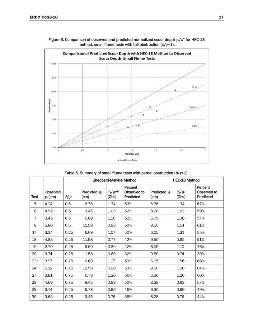
Experimental results for the small flume tests where the pier formed a full obstruction to flow throughout the entire water column (h/y=1) are shown in Table 4. Observed scour depths were consistently less than predicted scour depths, ranging from 46 to 78 percent of predicted values for the Sheppard-Melville method and 48 to 86 percent of predicted values for the HEC-18 method. It is possible that approach velocities closer to the sediment critical velocity (V/Vc ≈ 1) may have narrowed the difference between observed and predicted scour depths. However, the tested flow intensity parameters V/Vc = 0.66 to 0.76 are within the range considered for clear-water scour (0.4<V/Vc<1). Comparisons of observed and predicted normalized scour depth ys/a* for both the Sheppard-Melville and the HEC-18 methods are illustrated in Figures 5 and 6, respectively.

5.1.2 Results for small flume tests with partial obstructions (h/y<1)

Small flume tests with partial obstructions (h/y<1) were conducted to determine the reduction in observed scour depth due to only a portion of the flow depth’s being blocked by the submerged obstacle. The experimental results for these test configurations are listed in Table 5.

ERDC TR-16-10 15

Table 3. Experimental results for complete small flume test matrix.

Test Observed ys (cm)

Sheppard-Melville Method HEC-18 Method

Predicted ys (cm)

Ys/a*a (Obs)

Percent Observed to Predicted

Predicted ys (cm) Ys/aa (Obs)


1 4.15 6.78 1.31 61% 6.36 1.31 65%

2 5.57 9.45 1.17 59% 8.28 1.17 67%

3 2.52 5.53 0.79 46% 5.20 0.79 48%

4 3.43 7.51 0.72 46% 6.77 0.72 51%

5 4.24 6.78 1.34 63% 6.36 1.34 67%

6 4.92 9.45 1.03 52% 8.28 1.03 59%

7 3.45 6.69 1.10 52% 6.05 1.36 57%

8 5.80 11.58 0.93 50% 9.50 1.14 61%

9 3.35 6.69 1.07 50% 6.05 1.32 55%

10 4.92 11.58 0.79 42% 9.50 0.97 52%

11 3.88 6.69 1.24 58% 6.05 1.53 64%

12 5.95 11.58 0.95 51% 9.50 1.17 63%

13 3.49 6.69 1.12 52% 6.05 1.37 58%

14 5.02 11.58 0.80 43% 9.50 0.99 53%

15 3.56 6.69 1.14 53% 6.05 1.40 59%

16 5.46 11.58 0.87 47% 9.50 1.07 57%

17 3.34 6.69 1.07 50% 6.05 1.31 55%

18 4.83 11.58 0.77 42% 9.50 0.95 51%

19 2.79 6.69 0.89 42% 6.05 1.10 46%

20 3.74 11.58 0.60 32% 9.50 0.74 39%

23 b 3.97 6.69 1.27 59% 6.05 1.56 66%

24 6.12 11.58 0.98 53% 9.50 1.20 64%

25 5.22 6.69 1.67 78% 6.05 2.05 86%

26 7.40 11.58 1.18 64% 9.50 1.46 78%

27 3.81 6.78 1.20 56% 6.36 1.20 60%

28 4.69 9.45 0.98 50% 8.28 0.98 57%

29 3.14 6.78 0.99 46% 6.36 0.99 49%

30 3.63 9.45 0.76 38% 8.28 0.76 44%

31 4.06 6.78 1.28 60% 6.36 1.28 64%

32 5.12 9.45 1.08 54% 8.28 1.08 62%

33 2.11 6.78 0.66 31% 6.36 0.66 33%

34 2.74 9.45 0.57 29% 8.28 0.57 33% a a*=K × pier width, where K = 1 for cylindrical shapes, 1.23 for square shapes. b Tests 21 and 22 are purposely omitted due to missing bed scan data.

ERDC TR-16-10 16

Table 4. Summary of results for small flume tests with full obstruction (h/y=1).



Predicted ys (cm)

Ys/a*a (Obs)


Predicted ys (cm)

Ys/aa (Obs)


1 4.15 6.78 1.31 61% 6.36 1.31 65%

2 5.57 9.45 1.17 59% 8.28 1.17 67%

3 2.52 5.53 0.79 46% 5.20 0.79 48%

4 3.43 7.51 0.72 46% 6.77 0.72 51%

25 5.22 6.69 1.67 78% 6.05 2.05 86%

26 7.40 11.58 1.18 64% 9.50 1.46 78%

a a*=K × pier width, where K = 1 for cylindrical shapes, 1.23 for square shapes.

Figure 5. Comparison of observed and predicted normalized scour depth ys/a* for Sheppard-Melville method, small flume tests with full obstruction (h/y=1).

ERDC TR-16-10 17

Figure 6. Comparison of observed and predicted normalized scour depth ys/a* for HEC-18 method, small flume tests with full obstruction (h/y=1).

Table 5. Summary of small flume tests with partial obstruction (h/y<1).

Test Observed ys (cm) h/ya


Predicted ys (cm)

Ys/a*b (Obs)


Predicted ys (cm)

Ys/ab (Obs)


5 4.24 0.5 6.78 1.34 63% 6.36 1.34 67%

6 4.92 0.5 9.45 1.03 52% 8.28 1.03 59%

7 3.45 0.5 6.69 1.10 52% 6.05 1.36 57%

8 5.80 0.5 11.58 0.93 50% 9.50 1.14 61%

17 3.34 0.25 6.69 1.07 50% 6.05 1.31 55%

18 4.83 0.25 11.58 0.77 42% 9.50 0.95 51%

19 2.79 0.25 6.69 0.89 42% 6.05 1.10 46%

20 3.74 0.25 11.58 0.60 32% 9.50 0.74 39%

23 c 3.97 0.75 6.69 1.27 59% 6.05 1.56 66%

24 6.12 0.75 11.58 0.98 53% 9.50 1.20 64%

27 3.81 0.75 6.78 1.20 56% 6.36 1.20 60%

28 4.69 0.75 9.45 0.98 50% 8.28 0.98 57%

29 3.14 0.25 6.78 0.99 46% 6.36 0.99 49%

30 3.63 0.25 9.45 0.76 38% 8.28 0.76 44%

ERDC TR-16-10 18

Test Observed ys (cm) h/ya


Predicted ys (cm)

Ys/a*b (Obs)


Predicted ys (cm)

Ys/ab (Obs)


31 4.06 0.5 6.78 1.28 60% 6.36 1.28 64%

32 5.12 0.5 9.45 1.08 54% 8.28 1.08 62%

33 2.11 0.1 6.78 0.66 31% 6.36 0.66 33%

34 2.74 0.1 9.45 0.57 29% 8.28 0.57 33% a h/y = percentage of obstructed flow. h = height of obstruction, y = depth of flow. b a* = K × pier width, where K = 1 for cylindrical shapes, 1.23 for square shapes. c Tests 21 and 22 are purposely omitted due to missing bed scan data.

The consistent decrease in observed scour depth with decreasing flow obstruction percentage in comparison to scour depths for fully obstructed flow conditions is shown in Figure 7 and Figure 8 for both the Sheppard-Melville and the HEC-18 methods, respectively. The observed normalized scour depths ys/a* as a percentage of predicted ys/a* with the Sheppard-Melville method ranges from 59 percent for 0.75 flow obstruction to 29 percent for 0.1 flow obstruction. The observed normalized scour depths ys/a* as a percentage of predicted ys/a* with the HEC-18 method ranges from 66 percent for 0.75 flow obstruction to 33 percent for 0.1 flow obstruction.

Figure 7. Comparison of observed and predicted normalized scour depth ys/a* for Sheppard-Melville method, small flume tests with partial obstruction (h/y<1).

ERDC TR-16-10 19

Figure 8. Comparison of observed and predicted normalized scour depth ys/a* for HEC-18 method, small flume tests with partial obstruction (h/y<1).

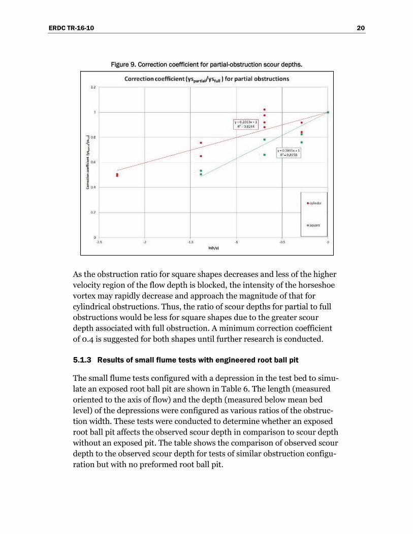
The ratio of observed scour depth for partial obstruction to observed scour depth for full obstruction was computed for each pier configuration and plotted versus the obstruction ratio h/y to determine the relationship between scour depth reduction and obstruction submergence. The resulting relationship describes a correction coefficient that can be applied by multiplication to scour depths predicted with the bridge pier scour methods to account for the decrease in scour depth due to a partial obstruction. The relationships are shown in Figure 9. The ratio of observed scour depth for partial obstruction to full obstruction was plotted against the natural log of the obstruction ratio h/y for both cylindrical and square obstruction shapes, and a linear regression was fitted to each dataset.

By definition, the regressions pass through unity at ln(h/y)=0 for fully obstructed flow. For cylindrical shapes, the correction coefficient is approximately 0.5 for the minimum value of h/y=0.1 that was tested. The regression for square obstruction shapes indicates a smaller correction factor than that for cylindrical obstruction shapes for a given value of h/y. This may be due to the greater fully obstructed scour depths for square shapes compared to cylindrical shapes. However, it may also indicate that obstructions with square-shaped faces deflect a greater percentage of the flow from the upper portion of the water column than cylindrical shapes, which increase the horseshoe vortex at the base of the obstruction and subsequently increase scour depths.

ERDC TR-16-10 20

Figure 9. Correction coefficient for partial-obstruction scour depths.

As the obstruction ratio for square shapes decreases and less of the higher velocity region of the flow depth is blocked, the intensity of the horseshoe vortex may rapidly decrease and approach the magnitude of that for cylindrical obstructions. Thus, the ratio of scour depths for partial to full obstructions would be less for square shapes due to the greater scour depth associated with full obstruction. A minimum correction coefficient of 0.4 is suggested for both shapes until further research is conducted.

5.1.3 Results of small flume tests with engineered root ball pit

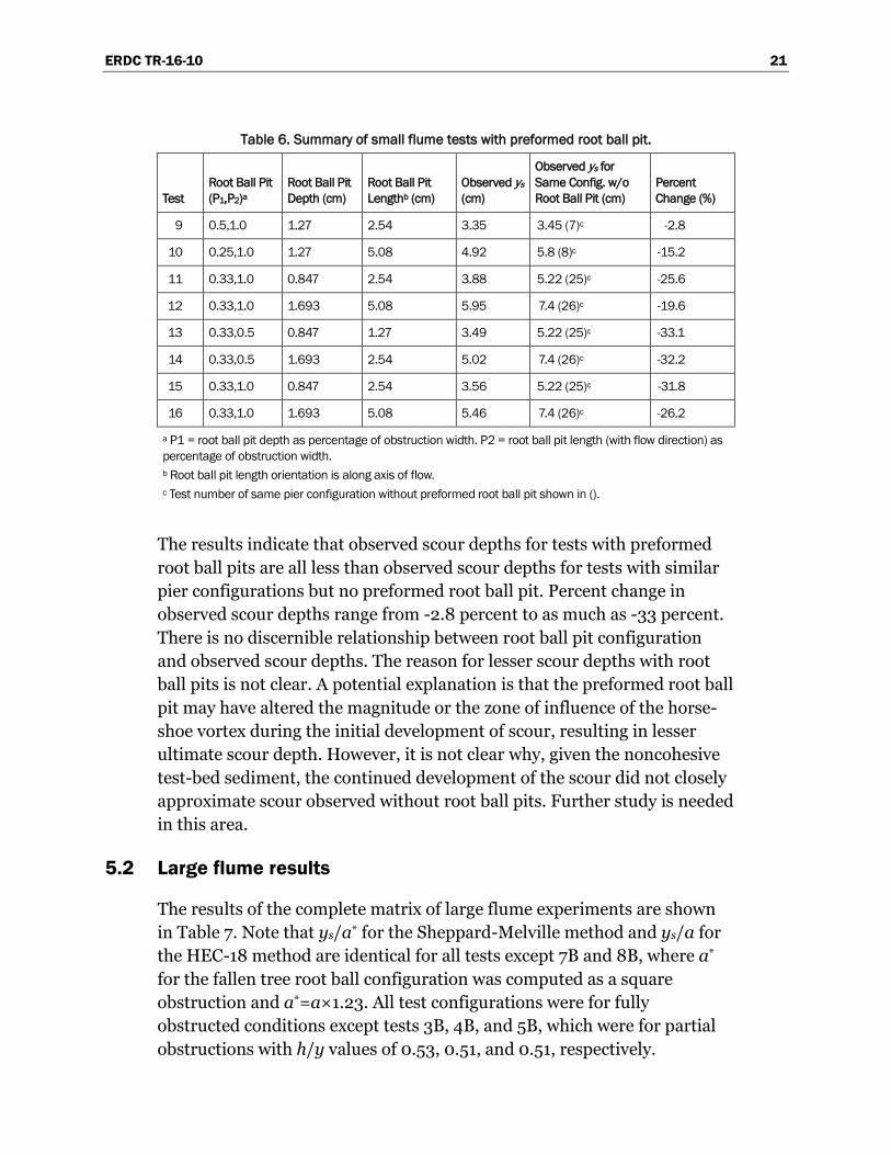
The small flume tests configured with a depression in the test bed to simu-late an exposed root ball pit are shown in Table 6. The length (measured oriented to the axis of flow) and the depth (measured below mean bed level) of the depressions were configured as various ratios of the obstruc-tion width. These tests were conducted to determine whether an exposed root ball pit affects the observed scour depth in comparison to scour depth without an exposed pit. The table shows the comparison of observed scour depth to the observed scour depth for tests of similar obstruction configu-ration but with no preformed root ball pit.

ERDC TR-16-10 21

Table 6. Summary of small flume tests with preformed root ball pit.

Test Root Ball Pit (P1,P2)a

Root Ball Pit Depth (cm)

Root Ball Pit Lengthb (cm)

Observed ys (cm)

Observed ys for Same Config. w/o Root Ball Pit (cm)

Percent Change (%)

9 0.5,1.0 1.27 2.54 3.35 3.45 (7)c -2.8

10 0.25,1.0 1.27 5.08 4.92 5.8 (8)c -15.2

11 0.33,1.0 0.847 2.54 3.88 5.22 (25)c -25.6

12 0.33,1.0 1.693 5.08 5.95 7.4 (26)c -19.6

13 0.33,0.5 0.847 1.27 3.49 5.22 (25)c -33.1

14 0.33,0.5 1.693 2.54 5.02 7.4 (26)c -32.2

15 0.33,1.0 0.847 2.54 3.56 5.22 (25)c -31.8

16 0.33,1.0 1.693 5.08 5.46 7.4 (26)c -26.2

a P1 = root ball pit depth as percentage of obstruction width. P2 = root ball pit length (with flow direction) as percentage of obstruction width. b Root ball pit length orientation is along axis of flow. c Test number of same pier configuration without preformed root ball pit shown in ().

The results indicate that observed scour depths for tests with preformed root ball pits are all less than observed scour depths for tests with similar pier configurations but no preformed root ball pit. Percent change in observed scour depths range from -2.8 percent to as much as -33 percent. There is no discernible relationship between root ball pit configuration and observed scour depths. The reason for lesser scour depths with root ball pits is not clear. A potential explanation is that the preformed root ball pit may have altered the magnitude or the zone of influence of the horse-shoe vortex during the initial development of scour, resulting in lesser ultimate scour depth. However, it is not clear why, given the noncohesive test-bed sediment, the continued development of the scour did not closely approximate scour observed without root ball pits. Further study is needed in this area.

5.2 Large flume results

The results of the complete matrix of large flume experiments are shown in Table 7. Note that ys/a* for the Sheppard-Melville method and ys/a for the HEC-18 method are identical for all tests except 7B and 8B, where a* for the fallen tree root ball configuration was computed as a square obstruction and a*=a×1.23. All test configurations were for fully obstructed conditions except tests 3B, 4B, and 5B, which were for partial obstructions with h/y values of 0.53, 0.51, and 0.51, respectively.

ERDC TR-16-10 22

Table 7. Experimental results for complete large flume test matrix.



Predicted ys (cm)

Ys/a* (Obs)


Predicted ys (cm) Ys/a (Obs)


1B 27.1 56.0 0.53 48.5 73.5 0.53 36.9

2B 38.7 87.7 0.42 44.1 107.7 0.42 35.9

3B 18.9 56.0 0.37 33.8 73.5 0.37 25.7

4B 25.9 87.7 0.28 29.5 107.7 0.28 24.0

5B 17.7 82.9 0.19 21.3 77.2 0.19 22.9

6B 23.8 82.9 0.26 28.7 77.2 0.26 30.8

7B1 13.1 95.7 0.11 13.7 87.8 0.14 14.9

8B 17.4 95.7 0.15 18.2 87.8 0.18 19.8

9B2 16.2 51.2 0.40 31.5 45.4 0.40 35.7

10B 17.1 51.2 0.42 33.4 45.4 0.42 37.6

1 Tree trunk floated during test 7B. Test 8B was a repeat of Test 7B with the tree trunk secured. 2 Test 9B terminated after 3 hr due to loss of flume pool. Test 10B was a repeat of Test 9B.

5.2.1 Results of large flume tests with full obstructions (h/y=1)

Large flume tests 1B, 2B, and 6B have a fully obstructed configuration for cylindrical pier shapes. Tests 7B through 10B were also full obstructions, but were for configurations with the actual tree and root ball and will be presented separately. In general, the observed scour depths for fully obstructed conditions were consistently less than predicted scour depths. As a percentage of predicted scour depth, observed scour depths were less for the large flume tests than for the small flume tests. Observed scour depths as a percentage of scour depths predicted with the Sheppard-Melville method range from 28.7 to 48.5 percent. Observed scour depths as a percentage of scour depths predicted with the HEC-18 method range from 30.8 to 36.9 percent. Comparison of observed and predicted normalized scour depth ys/a* for the Sheppard-Melville method is shown in Figure 10 for the large flume tests with the small flume tests’ results included for comparison. Likewise, comparison of observed and predicted normalized scour depth ys/a for the HEC-18 method is shown in Figure 11. Both methods significantly over-predicted scour depths for the large flume tests by approximately 50 to 75 percent.

ERDC TR-16-10 23

Figure 10. Comparison of observed and predicted normalized scour depths for Sheppard-Melville method, small and large flume tests.

Figure 11. Comparison of observed and predicted normalized scour depths for HEC-18 method, small and large flume tests.

ERDC TR-16-10 24

5.2.2 Results of large flume tests with partial obstructions (h/y<1)

Large flume tests 3B, 4B, and 5B were for partially obstructed cases with h/y values of 0.53, 0.51, and 0.51, respectively. The ratio of observed scour depth for these cases to observed depths for similarly configured tests with full obstruction was 0.70, 0.67, and 0.74, respectively. Based on the correction-factor curves developed with the small flume test results, the ratio of scour depths for partial to full obstruction for the large flume tests should have been 0.87, 0.86, and 0.86, respectively (based on the curve for cylindrical obstructions). The ratios are shown in comparison to those of the small flume tests in Figure 12. In general, the test results for the large flume, which were all cylinder-shaped piers, are in better agreement with the curve for the square-shaped obstructions. However, the general agreement is reasonable, and the trend of reduced scour depth for partial obstructions for the large flume tests is similar to that observed in the small flume tests.

Figure 12. Comparison of partial obstruction correction factors for small and large flume tests.

ERDC TR-16-10 25

5.2.3 Results of large flume tests with tree/root ball

Large flume tests 7B, 8B, 9B, and 10B were conducted with a real tree with an intact root ball. Tests 7B and 8B were with the tree in a fallen configuration and the root ball providing a complete obstruction of the flow field, while tests 9B and 10B were with the tree in a standing configuration with the trunk of the tree acting as a bridge pier. These tests were conducted to gain limited insight into how scour depth caused by the tree obstruction compares to scour depths predicted using the bridge pier scour models. It was clear that deployment of the tree in the test bed would only grossly approximate conditions of a tree in situ at best. However, the tests were conducted to gain at least a general idea of scour characteristics involving the tree and root ball. In the case of the standing-tree configured tests, there was a discontinuity at the interface between the sand test bed and the cohesive material in the root ball. This discontinuity was unavoidable in terms of test-bed preparation. Additionally, there was an abrupt cutoff in the root system at this interface because many of the roots normally in place for standing trees were not attached to the root ball. In the case of the fallen tree test configurations, the test bed was completely level and contained no preformed root ball pit.

The observed scour depths for tests 7B and 8B were 13.1 cm and 17.4 cm, respectively. Given a width of 0.96 m and assuming a square shape factor of 1.23 for the root ball, the observed normalized scour depths ys/a*, in terms of the Sheppard-Melville method for tests 7B and 8B, were 0.15 and 0.11, respectively. The observed normalized scour depths ys/a in terms of the HEC-18 method for tests 7B and 8B were 0.14 and 0.18, respectively. For the Sheppard-Melville method, the observed scour depths were approximately 14 percent and 18 percent of predicted values for tests 7B and 8B, respectively. For the HEC-18 method, the observed scour depths were approximately 15 percent and 20 percent of predicted values for tests 7B and 8B, respectively. The observed scour depths as a percentage of predicted scour depths for the fallen tree/root ball configurations were much less than those for the small flume experiments and the other large flume experiments. One explanation for the lesser observed scour depths with these tests is that the roughness of the irregular root ball surface may introduce turbulence that prevents the downward plunging jet from fully forming, thus reducing scour depth. In addition, as material is washed away from the root ball, the “obstruction” becomes more porous and flow passes through the root ball instead of being deflected by it. This has the effect of reducing the width of the flow obstruction.

ERDC TR-16-10 26

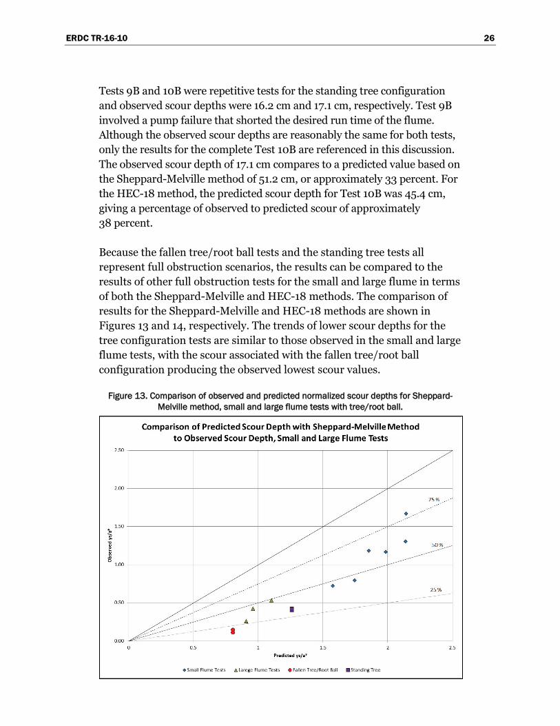
Tests 9B and 10B were repetitive tests for the standing tree configuration and observed scour depths were 16.2 cm and 17.1 cm, respectively. Test 9B involved a pump failure that shorted the desired run time of the flume. Although the observed scour depths are reasonably the same for both tests, only the results for the complete Test 10B are referenced in this discussion. The observed scour depth of 17.1 cm compares to a predicted value based on the Sheppard-Melville method of 51.2 cm, or approximately 33 percent. For the HEC-18 method, the predicted scour depth for Test 10B was 45.4 cm, giving a percentage of observed to predicted scour of approximately 38 percent.

Because the fallen tree/root ball tests and the standing tree tests all represent full obstruction scenarios, the results can be compared to the results of other full obstruction tests for the small and large flume in terms of both the Sheppard-Melville and HEC-18 methods. The comparison of results for the Sheppard-Melville and HEC-18 methods are shown in Figures 13 and 14, respectively. The trends of lower scour depths for the tree configuration tests are similar to those observed in the small and large flume tests, with the scour associated with the fallen tree/root ball configuration producing the observed lowest scour values.

Figure 13. Comparison of observed and predicted normalized scour depths for Sheppard-Melville method, small and large flume tests with tree/root ball.

ERDC TR-16-10 27

Figure 14. Comparison of observed and predicted normalized scour depths for HEC-18 method, small and large flume tests with tree/root ball.

ERDC TR-16-10 28

6 Discussion of Applicability to Large Woody Vegetation Scour

As stated previously, the objective of these flume validation experiments was to develop methods and guidance for application of existing bridge pier scour equations to the case of tree scour, particularly as it relates to evaluation of scour effects on levee integrity and safety. The results of the flume experiments provide limited information in terms of standing tree scour, as the tests could not address the effect of the tree root system on potential scour depth. Further research is needed to adequately quantify the effect of tree roots on scour.

6.1 Application to the standing tree case

Approximation of scour associated with flow around standing trees with bridge pier scour predictor methods appears to be very conservative in terms of evaluation of tree scour effects on levee integrity and safety. The results of the flume experiments indicate, in general, the Sheppard-Melville and HEC-18 methods both tend to over-predict observed scour depths as much as 25 to 75 percent. This tendency for over-prediction of scour depths, coupled with potential reduction in scour due to the root system, suggests that these bridge scour methods could be used with reasonable assurance to approximate maximum scour associated with standing trees. Although the Sheppard-Melville and HEC-18 methods were the only ones investigated, it can be reasonably assumed that other bridge scour predictors may also be used to approximate maximum scour depths for standing trees.

For standing trees with very little trunk taper, the diameter breast height (DBH) of the tree provides a reasonable approximation of the pier width for use in the bridge scour equations. The effective pier width can be considered equal to the DBH (i.e., a pier shape factor of 1). For standing trees with a significant taper where the tree diameter at the base (ground surface) is larger than the DBH, an average or representative tree diameter should be computed. For purposes of the large flume experiments with the standing tree, an “effective” diameter was determined that produced the same area of obstruction for the full flow depth as did the tapered tree trunk. This method provides a reasonable estimation of the tree width to

ERDC TR-16-10 29

be used in the bridge pier scour equations. Depending on the nature of the tree trunk taper and shape near the ground surface, a square shape factor of 1.23 may be applicable. Irregularities in tree trunk shape and width can make the determination of a representative pier width problematic.

6.2 Application to fallen tree/root ball case

For the case of a fallen tree where the upturned root ball creates an obstruction to the full flow depth, the width of the root ball can be used as the pier width, and the bridge pier scour equations can be used in the same manner as for the case of a standing tree. Unless the shape of the exposed root ball dictates otherwise, it is suggested to consider the root ball a square shape obstruction and use a shape factor of 1.23 to compute the effective width = root ball width × 1.23. It should be assumed that the width of the root ball is perpendicular to the direction of flow. Given the results of the research reported herein, no adjustment or correction for an exposed root ball pit is suggested at this time. Additional research in this area is suggested.

For situations in which the upturned root ball creates only a partial obstruction of the flow depth, scour depths determined with the bridge pier scour equations should be reduced by a correction factor such that

s sy partial y full COEF (4)

where

ys(partial) = scour depth when root ball is submerged and creates a partial obstruction to flow

ys(full) = scour depth computed from bridge pier scour equation

COEF = correction coefficient for partial obstruction

The correction coefficient COEF is based on the results of the small flume experiments for partial obstruction and is given by

. hCOEF lny

0 2013 1 (for cylindrical shapes), or

ERDC TR-16-10 30

. hCOEF lny

0 3691 1 (for square shapes)

where

h = height of root ball obstruction y = depth of flow

Based on the small flume experimental results, a minimum COEF value of 0.4 is suggested at this time for both cylindrical and square shapes.

ERDC TR-16-10 31

7 Summary and Recommendations

Thirty-four small flume and 10 large flume clear-water scour experiments were conducted to determine the applicability of existing bridge pier scour equations in evaluating scour effects of large woody vegetation (i.e., trees). Experimental results were used to develop additional guidance for determining scour impacts of trees on or near flood-control levees as part of levee safety and integrity assessments. The experimental test matrix included piers with cylindrical and square shapes that fully and partially obstructed the flow depth. Tests of an actual tree with an intact root ball were conducted with both standing tree and fallen tree configurations.

Both the Sheppard-Melville and HEC-18 methods of bridge pier scour prediction were evaluated for performance in terms of over- or under-prediction of scour depths. Results from the small and large flumes indicate both methods consistently over-predict scour depth as much as 25 to 75 percent. Flume tests involving a realistic standing tree indicate over-prediction of scour depths are similar to those observed for idealized cylinders/piers. Although other bridge pier scour methods can be used, both the Sheppard-Melville and HEC-18 methods can be used in assessing tree scour potential to conservatively estimate maximum scour that may occur.

The effect of partial obstructions on reduction of scour depth was investigated. Experiment results indicate reduction in observed depth for partial obstructions as compared to scour depth for fully obstructed flow is a function of the ratio of obstructed height to flow depth h/y. Relationships were developed for correction factors to use with scour depths computed with bridge pier scour equations to estimate scour for partial obstructions.

The following recommendations are made for application of bridge pier scour methods to estimate tree scour as part of levee integrity and safety assessment:

1. Bridge pier scour methods can be reasonably applied for standing tree scour prediction by assuming the tree acts as a bridge pier. For a tree with uniform diameter and little trunk taper, the DBH of the tree can be used as the pier width in the computations. For tree trunks with a significant taper,

ERDC TR-16-10 32

an effective diameter that produces an equivalent area of obstruction should be used.

2. For the case of a fallen tree with an upturned root ball that is not submerged and does not fully obstruct the flow, the bridge pier scour equations can be used, assuming the root ball acts as a bridge pier with a width equal to the root ball width. Adjustment of the pier width with an applicable shape factor may be required, based on the general shape of the root ball.

3. For the case in which the root ball is submerged and creates a partial obstruction to flow, the scour depth should be estimated by applying a correction factor to the scour depth determined from the prediction equations such that ys(partial) = COEF × ys(full). The value of COEF is a function of the ratio of obstruction height to flow depth h/y. For cylindrical obstructions, COEF = 0.2013×ln(h/y)+1, and for square-shaped obstructions COEF = 0.3691×ln(h/y)+1. A minimum value of COEF = 0.4 is suggested for both shapes.

4. At this time, no correction for the effect of existing root ball pits is suggested. Further investigation is recommended for this situation.

ERDC TR-16-10 33

References American Society of Civil Engineers (ASCE). 2008. ASCE Manuals and Reports on

Engineering Practice 110, Sedimentation engineering: processes, management, modeling, and practice. Marcel H. Garcia, editor.

Ettema, R., G. Constantinescu, and B. Melville. 2011. Evaluation of bridge scour research: Pier scour processes and prediction. National Highway Cooperative Research Program (NCHRP). http://onlinepubs.trb.org/onlinepubs/ nchrp/nchrp_w175.pdf.

Melville, B. W. 1997. Pier and abutment scour: integrated approach. ASCE. Journal of the Hydraulic Division 123(2):125-136.

Richardson, E. V., and S. R. Davis. 1995. Evaluating scour at bridges. 3rd ed. HEC 18 Publication FHWA-IP-90-017. Washington, DC: U.S. Department of Transportation.

______. 2001. Evaluating scour at bridges. 4th ed. Report No FHWA NHI 01-001, Hydraulic Engineering Circular No. 18. Washington, DC: U.S. Department of Transportation.

Sheppard, D. M., H. Demir, and B. Melville. 2011. Scour at wide piers and long skewed piers. NCHRP Report 682. Washington, DC: Transportation Research Board.

Sheppard, D. M., and W. Miller. 2006. Live-bed local pier scour experiments. Journal of Hydraulic Engineering 132(7):635-642.

Yuill, B. (In preparation). Review of existing bridge scour models and evaluation of model applicability for use in tree scour prediction on levees. Draft report. Vicksburg, MS: U.S. Army Engineer and Research Development Center.

http://onlinepubs.trb.org/onlinepubs/nchrp/nchrp_w175.pdf

http://onlinepubs.trb.org/onlinepubs/nchrp/nchrp_w175.pdf

ERDC TR-16-10 34

Appendix A: Small Flume Experiments

Thirty-four tests were conducted in a tilting flume, measuring 24.5 m long by 0.91 m wide by 0.3 m deep. A test section of silica sand, measuring 8.44 m long by 0.11 m deep with a D50 of 0.52 mm, was placed in the model as shown in Figure A-1. Initially, the model consisted of a 7.92-m- by 0.3-m- deep approach, a 0.6-m-long cutoff section, a 4.76-cm-diam cylinder, a 3.18-cm-diam cylinder followed by 2.44 m of sand, a 0.98-m cutoff section, and a 6.1-m- by 0.3-m-deep exit channel.

Two obstruction geometries, cylindrical and square, of varying heights were tested in the model (Figure A-2). The obstructions were placed through the full depth of the sand 3 m apart on centers. The cylinders were standard schedule C polyvinyl chloride (PVC), and the squares were fabri-cated of Plexiglas painted with a white finish. Roughness or irregularities of obstruction surfaces may result in different scour depths.

A.1 Appurtenances and instrumentation

Water used in the operation of the model was supplied by a pump, and dis-charges were measured with a venturi meter. The tailwater downstream of the model was controlled by an adjustable tailgate. Steel rails set to grade provided reference planes. Water surface elevations were obtained with a point gauge 3 m downstream at the end of the test section. Velocities were measured with a Nixon 402 digital flowmeter with a propeller-type probe (Figure A-4) 0.6 m upstream of each obstruction. A handheld laser scanner (Figure A-5) was used to map the contours of the resulting scour holes. The laser scanner reference plane is shown in Figure A-6. The sorting effect that can occur in the scour phenomenon was eliminated by the use of closely graded silica sand having the mean size of 0.52 mm and the size distribution shown in Figure A-3.

A.2 Experiment procedure

Critical velocity was calculated based on the FHWA HEC-18 clear-water scour equation (Richardson and Davis 2001) (Equation A-1). The maximum average velocity in the model was set equal to 75 percent of Vc.

/ /c uV K y D

1 6 1 350 (A.1)

ERDC TR-16-10 35

where:

Vc = Critical velocity, clear-water scour velocity, m/s Ku = 6.19, SI units y = flow depth, m D50 = median particle size, mm.

With the tailgate in its highest position and the flume filled with water, the flow was fixed at 0.04 m3/s, a condition that did not cause movement of the sand. The tailgate was then gradually lowered until a depth of flow of 15.24 cm was reached with an approach velocity of 27.43 cm/s. The times of starting, initial movement, and water surface were recorded. The average velocity was measured at 1-hr intervals using the Nixon 402 digital flowmeter 0.6 m upstream of each obstruction. Scour elevation was documented at 1-hr intervals using a scale drawn on each obstruction until the scour hole stabilized. At the end of 3 hr, the tailgate was raised until the sand movement ceased. The supply valve was then closed, and the water was drained from the flume. Photographs and video recorded the process. This procedure was adopted except where noted.

The percentage of flow depth obstructed and correlating submergences and descriptions of test conditions for cylindrical and square obstructions are tabulated in Tables A-1 and A-2, respectively. A comparison of photo and scanned images is shown in Figure A-7. Scour depth measurements were obtained using the coordinates on the scanned images. Photographs of resulting scour holes for each test with cylindrical obstructions and square obstructions are documented in Figure A-8 through A-17 and Figure A-18 through A-35, respectively.

ERDC TR-16-10 36

Figu

re A

-1. O

rigin

al m

odel

con

figur

atio

n.

ERDC TR-16-10 37

Figure A-2. Cylindrical and square obstructions.

ERDC TR-16-10 38

Figu

re A

-3. M

odel

san

d gr

adat

ion.

ERDC TR-16-10 39

Figure A-4. Nixon 402 digital flowmeter.

Velocity probe

ERDC TR-16-10 40

Figure A-5. Handheld laser scanner and scanning apparatus.

Figure A-6. Laser scanner reference plane.

Handheld laser scanner

ERDC TR-16-10 41

Figure A-7a. Photograph image of scour.

Figure A-7b. Laser scan image of scour.

ERDC TR-16-10 42

Table A-1. Small flume scour test matrix for cylindrical obstructions.

Test No. Obstruction

Obstruction Diameter, cm

Discharge Q, m3/s

Average, Velocity, cm/s

Flow Depth, cm

Submergence, cm

Flow Depth Obstructed, %

1 Cylinder 3.18 0.04 27.43 15.24 0 100

2 Cylinder 4.76 0.04 27.43 15.24 0 100

3 Cylinder 3.18 0.02 0.21 7.62 0 100

4 Cylinder 4.76 0.02 0.21 7.62 0 100

5 Cylinder 3.18 0.04 27.43 15.24 7.62 50

6 Cylinder 4.76 0.04 27.43 15.24 7.62 50

27 Cylinder 3.18 0.04 27.43 15.24 3.81 75

28 Cylinder 4.76 0.04 27.43 15.24 3.81 75

29 Cylinder 3.18 0.04 27.43 15.24 11.43 25

30 Cylinder 4.76 0.04 27.43 15.24 11.43 25

31 Cylinder 3.18 0.04 27.43 15.24 7.62 50

32 Cylinder 4.76 0.04 27.43 15.24 7.62 50

33 Cylinder 3.18 0.04 27.43 15.24 13.72 10

34 Cylinder 4.76 0.04 27.43 15.24 13.72 10

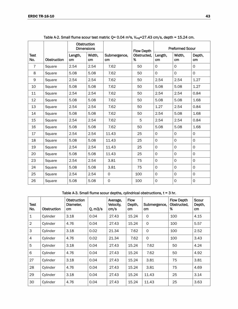
ERDC TR-16-10 43

Table A-2. Small flume scour test matrix: Q= 0.04 m3s, Vavg=27.43 cm/s, depth = 15.24 cm.


Obstruction Dimensions

Submergence, cm


Preformed Scour

Length, cm

Width, cm

Length, cm

Width, cm

Depth, cm

7 Square 2.54 2.54 7.62 50 0 0 0

8 Square 5.08 5.08 7.62 50 0 0 0

9 Square 2.54 2.54 7.62 50 2.54 2.54 1.27

10 Square 5.08 5.08 7.62 50 5.08 5.08 1.27

11 Square 2.54 2.54 7.62 50 2.54 2.54 0.84

12 Square 5.08 5.08 7.62 50 5.08 5.08 1.68

13 Square 2.54 2.54 7.62 50 1.27 2.54 0.84

14 Square 5.08 5.08 7.62 50 2.54 5.08 1.68

15 Square 2.54 2.54 7.62 5 2.54 2.54 0.84

16 Square 5.08 5.08 7.62 50 5.08 5.08 1.68

17 Square 2.54 2.54 11.43 25 0 0 0

18 Square 5.08 5.08 11.43 25 0 0 0

19 Square 2.54 2.54 11.43 25 0 0 0

20 Square 5.08 5.08 11.43 25 0 0 0

23 Square 2.54 2.54 3.81 75 0 0 0

24 Square 5.08 5.08 3.81 75 0 0 0

25 Square 2.54 2.54 0 100 0 0 0

26 Square 5.08 5.08 0 100 0 0 0

Table A-3. Small flume scour depths, cylindrical obstructions, t = 3 hr.


Obstruction Diameter, cm Q, m3/s

Average, Velocity, cm/s

Flow Depth, cm

Submergence, cm


Scour Depth, cm

1 Cylinder 3.18 0.04 27.43 15.24 0 100 4.15

2 Cylinder 4.76 0.04 27.43 15.24 0 100 5.57

3 Cylinder 3.18 0.02 21.34 7.62 0 100 2.52

4 Cylinder 4.76 0.02 21.34 7.62 0 100 3.43

5 Cylinder 3.18 0.04 27.43 15.24 7.62 50 4.24

6 Cylinder 4.76 0.04 27.43 15.24 7.62 50 4.92

27 Cylinder 3.18 0.04 27.43 15.24 3.81 75 3.81

28 Cylinder 4.76 0.04 27.43 15.24 3.81 75 4.69

29 Cylinder 3.18 0.04 27.43 15.24 11.43 25 3.14

30 Cylinder 4.76 0.04 27.43 15.24 11.43 25 3.63

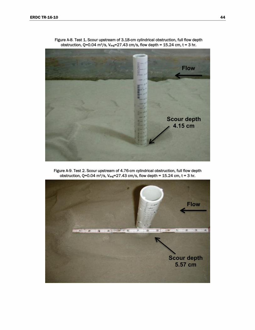
ERDC TR-16-10 44

Figure A-8. Test 1. Scour upstream of 3.18-cm cylindrical obstruction, full flow depth obstruction, Q=0.04 m3/s, Vavg=27.43 cm/s, flow depth = 15.24 cm, t = 3 hr.


Flow

Scour depth 5.57 cm

Scour depth 4.15 cm

Flow

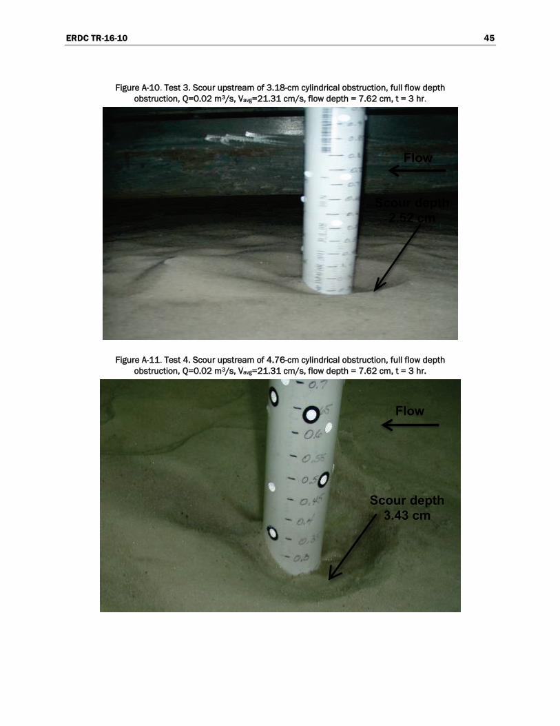
ERDC TR-16-10 45



Flow

Scour depth 3.43 cm

Scour depth 2.52 cm

Flow

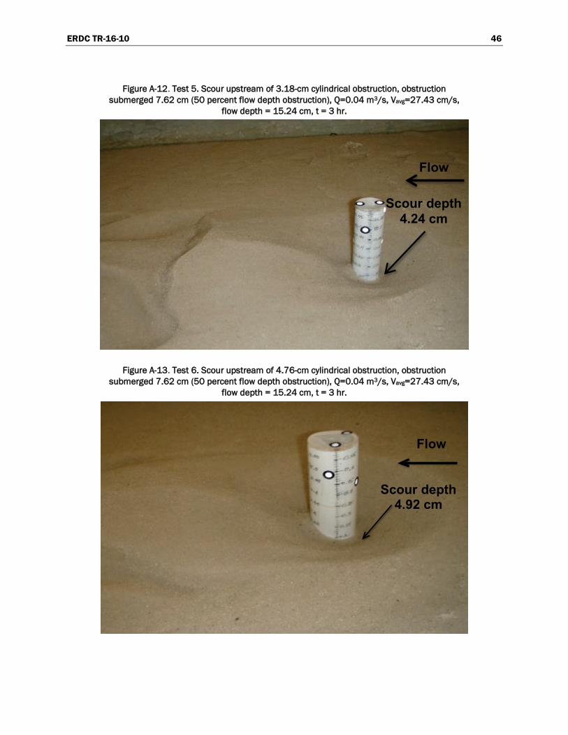
ERDC TR-16-10 46

Figure A-12. Test 5. Scour upstream of 3.18-cm cylindrical obstruction, obstruction submerged 7.62 cm (50 percent flow depth obstruction), Q=0.04 m3/s, Vavg=27.43 cm/s,

flow depth = 15.24 cm, t = 3 hr.



Scour depth 4.92 cm

Flow

Flow

Scour depth 4.24 cm

ERDC TR-16-10 47





Flow

Scour depth 4.69 cm

Scour depth 3.81 cm

Flow

ERDC TR-16-10 48

Figure A-16. Test 29. Scour upstream of 3.18-cm cylindrical obstruction obstruction submerged 11.43 cm (25 percent flow depth obstruction), Q=0.04 m3/s, Vavg=27.43 cm/s,


Flow

Scour depth 3.14 cm

ERDC TR-16-10 49



t = 0 hr t = 3 hr

Scour depth 3.63 cm

Flow

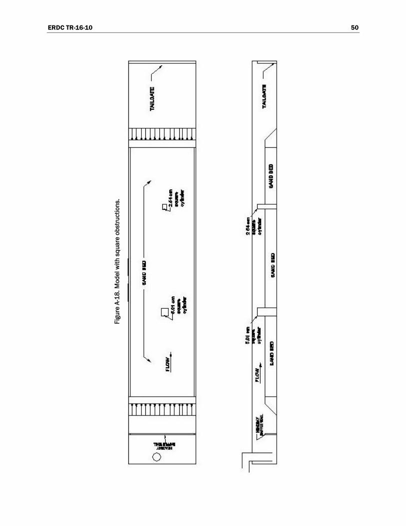
ERDC TR-16-10 50

Figu

re A

-18.

Mod

el w

ith s

quar

e ob

stru

ctio

ns.

ERDC TR-16-10 51

Figure A-19a. Test 7. Scour upstream of 2.54-cm-square obstruction, obstruction

submerged 7.62 cm (50 percent flow depth obstruction), t = 0 hr.

Figure A-19b. Test 7. Q=0.04 m3/s, Vavg=27.43 cm/s, flow depth = 15.24 cm, t = 3 hr.

Flow

Scour depth 3.45 cm

ERDC TR-16-10 52


submerged 7.62 cm (50 percent flow depth obstruction), t = 0 hr.


Scour depth 5.80 cm

Flow

ERDC TR-16-10 53

Figu

re A

-21.

Squ

are

obst

ruct

ions

with

pre

form

ed s

cour

hol

es.

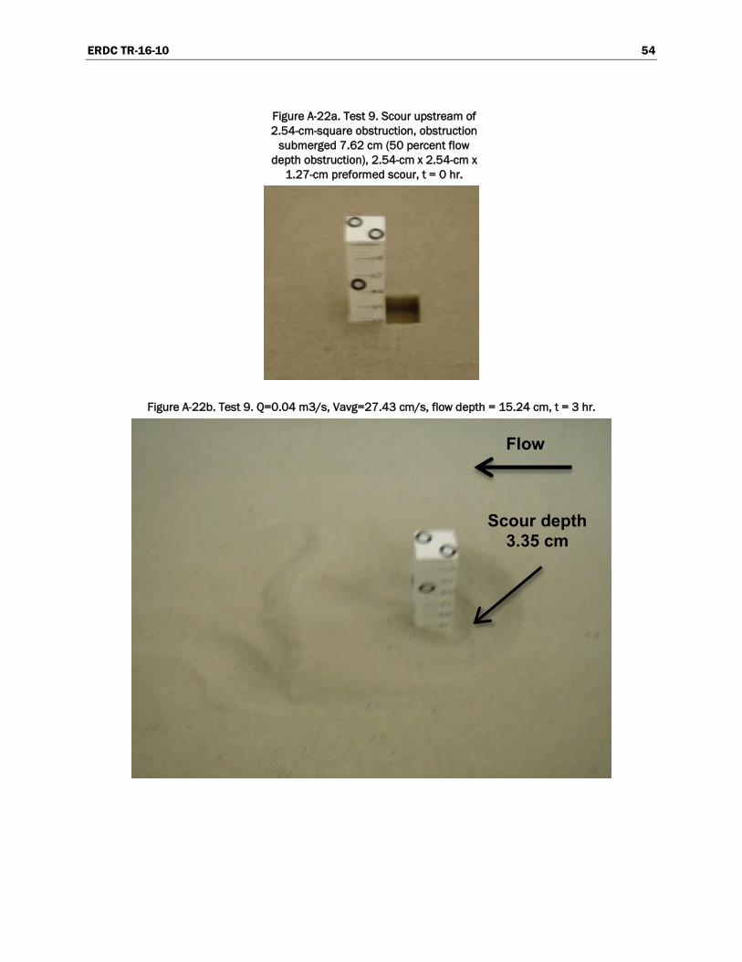
ERDC TR-16-10 54


submerged 7.62 cm (50 percent flow depth obstruction), 2.54-cm x 2.54-cm x

1.27-cm preformed scour, t = 0 hr.


Scour depth 3.35 cm

Flow

ERDC TR-16-10 55

Figure A-23a. Test 10. Scour upstream of 5.08-cm-square obstruction, obstruction submerged 7.62 cm

(50 percent flow depth obstruction), 5.08-cm x 5.08-cm x 1.27-cm preformed scour, t = 0 hr.

Figure A-24b. Q=0.04 m3/s, Vavg=27.43 cm/s, flow depth = 15.24 cm, t = 3 hr.

Scour depth 4.92 cm

Flow

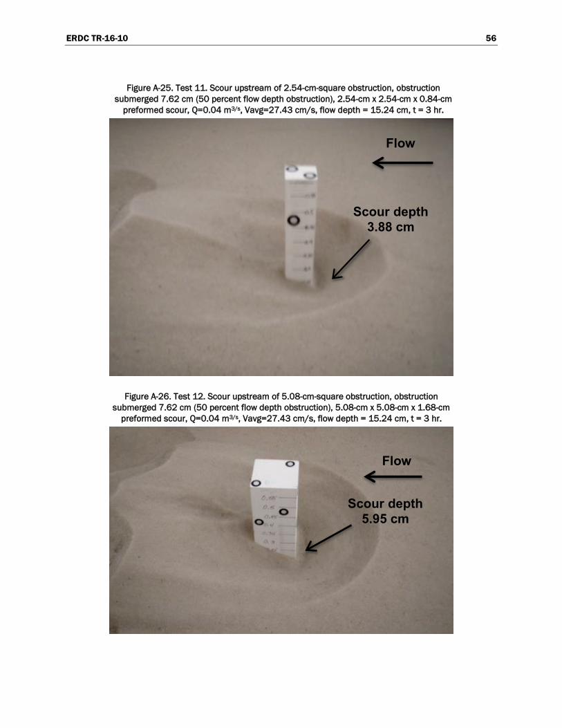
ERDC TR-16-10 56

Figure A-25. Test 11. Scour upstream of 2.54-cm-square obstruction, obstruction submerged 7.62 cm (50 percent flow depth obstruction), 2.54-cm x 2.54-cm x 0.84-cm

preformed scour, Q=0.04 m3/s, Vavg=27.43 cm/s, flow depth = 15.24 cm, t = 3 hr.



Flow

Scour depth 5.95 cm

Flow

Scour depth 3.88 cm

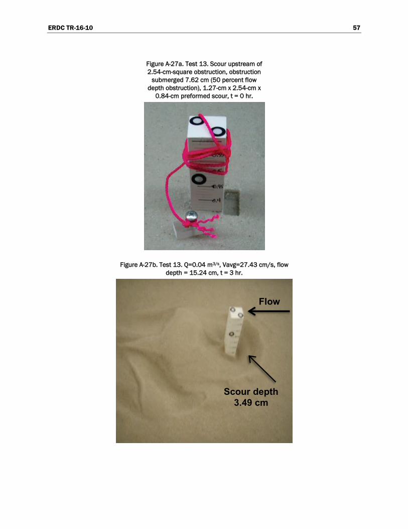
ERDC TR-16-10 57


submerged 7.62 cm (50 percent flow depth obstruction), 1.27-cm x 2.54-cm x

0.84-cm preformed scour, t = 0 hr.


Flow

Scour depth 3.49 cm

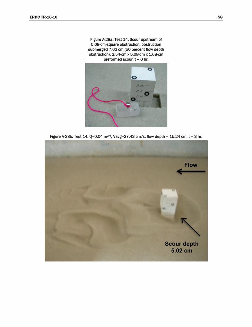
ERDC TR-16-10 58


submerged 7.62 cm (50 percent flow depth obstruction), 2.54-cm x 5.08-cm x 1.68-cm

preformed scour, t = 0 hr.


Flow

Scour depth 5.02 cm

ERDC TR-16-10 59


preformed scour, Q=0.04 m3/s, Vavg=27.43 cm/s, flow depth = 15.24 cm, t= 3 hr.



Flow

Scour depth

Scour depth

Flow

3.56 cm

5.46 cm

ERDC TR-16-10 60

Figure A-31. Test 17. Scour upstream of 2.54-cm-square obstruction, obstruction submerged 11.43 cm (25 percent flow depth obstruction), Q=0.04 m3/s, Vavg=27.43 cm/s, flow depth =

15.24 cm, t = 3 hr.


15.24 cm, t = 3 hr.

Flow

Scour depth 4.83 cm

Scour depth 3.34 cm

Flow

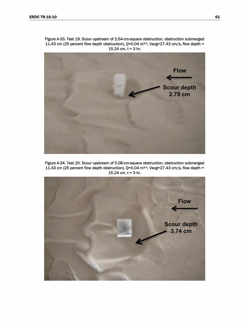
ERDC TR-16-10 61


15.24 cm, t = 3 hr.


15.24 cm, t = 3 hr.

Flow

Scour depth 3.74 cm

Flow

Scour depth 2.79 cm

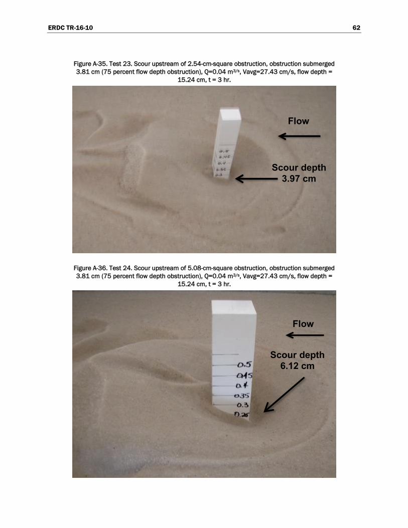
ERDC TR-16-10 62


15.24 cm, t = 3 hr.


15.24 cm, t = 3 hr.

Scour depth 6.12 cm

Flow

Scour depth 3.97 cm

Flow

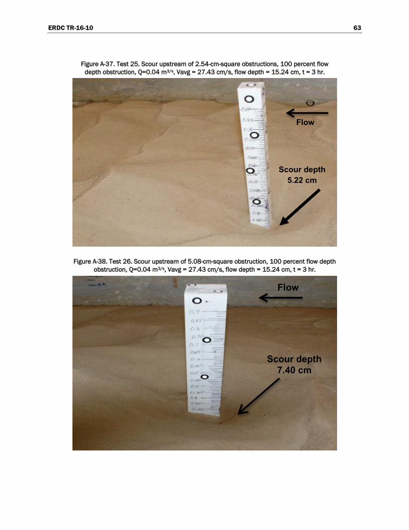
ERDC TR-16-10 63

Figure A-37. Test 25. Scour upstream of 2.54-cm-square obstructions, 100 percent flow depth obstruction, Q=0.04 m3/s, Vavg = 27.43 cm/s, flow depth = 15.24 cm, t = 3 hr.

Figure A-38. Test 26. Scour upstream of 5.08-cm-square obstruction, 100 percent flow depth obstruction, Q=0.04 m3/s, Vavg = 27.43 cm/s, flow depth = 15.24 cm, t = 3 hr.

Scour depth 7.40 cm

Flow

Scour depth 5.22 cm

Flow

ERDC TR-16-10 64

Table A-4. Small flume scour depths, square obstructions, Q=0.04 m3/s, Vavg=27.43 cm/s, depth = 15.24 cm, t = 3 hr.


Length, cm

Width, cm

Submergence, cm


Preformed Scour

Scour Depth, cm

Length, cm

Width, cm

Depth, cm

7 Square 2.54 2.54 7.62 50 0 0 0 3.45

8 Square 5.08 5.08 7.62 50 0 0 0 5.80

9 Square 2.54 2.54 7.62 50 2.54 2.54 1.27 3.35

10 Square 5.08 5.08 7.62 50 5.08 5.08 1.27 4.92

11 Square 2.54 2.54 7.62 50 2.54 2.54 0.84 3.88

12 Square 5.08 5.08 7.62 50 5.08 5.08 1.68 5.95

13 Square 2.54 2.54 7.62 50 1.27 2.54 0.84 3.49

14 Square 5.08 5.08 7.62 50 2.54 5.08 1.68 5.02

15 Square 2.54 2.54 7.62 5 2.54 2.54 0.84 3.56

16 Square 5.08 5.08 7.62 50 5.08 5.08 1.68 5.46

17 Square 2.54 2.54 11.43 25 0 0 0 3.34

18 Square 5.08 5.08 11.43 25 0 0 0 4.83

19 Square 2.54 2.54 11.43 25 0 0 0 2.79

20 Square 5.08 5.08 11.43 25 0 0 0 3.74

23 Square 2.54 2.54 3.81 75 0 0 0 3.97

24 Square 5.08 5.08 3.81 75 0 0 0 6.12

25 Square 2.54 2.54 0 100 0 0 0 5.22

26 Square 5.08 5.08 0 100 0 0 0 7.40

A.3 Results

In the small flume experiments, 34 tests were conducted in the study of the scour depth resulting from various submergences and geometric-shaped obstructions. The 3.18- and 4.76-cm-diam cylinders of varying heights were partially and totally submerged, and the resulting scours were recorded using a handheld laser scanner (Tests 1-6 and 27-32). The results of these tests indicate scour depth was greater upstream of the 4.76-cm-diam cylinder than the scour depth upstream of the 3.18-cm-diam cylinder for each flow condition. The scour depth was greatest when flow depth was fully obstructed (4.15 and 5.57 cm for the 3.18- and 4.76-cm-diam cylinders, respectively). As the cylinder depth of submergence increased or cylinder obstruction decreased (i.e., cylinder height decreased), the depth of scour decreased. Square obstructions of

ERDC TR-16-10 65

varying heights (2.54 and 5.08 cm) were partially and totally submerged, and the resulting scours were recorded using a handheld laser scanner (Tests 7-16, 19-20 and 23-26). The results of these tests indicate scour depth was greater upstream of the 5.08-cm-square obstruction than the scour depth upstream of the 2.54-cm-square obstruction for each flow condition. The scour depth was greatest when flow depth was fully obstructed (5.22 cm and 7.4 cm for the 2.54- and 5.08-cm-square obstructions, respectively). As the square obstruction’s depth of sub-mergence increased or the obstruction of flow decreased (i.e., square obstruction height decreased), the depth of scour decreased. Scour depth upstream of the square obstructions was consistently greater than the scour depth upstream of the cylinders for each size and concurrent flow condition. Based on the results, scour depths increase with increased angularity and size of obstructions and decrease of submergence.

ERDC TR-16-10 66

Appendix B: Large Flume Experiments

B.1 The Model and Experiments Procedure

B.1.1 Description

The large scale scour flume at ERDC was chosen for this research for its size and flow capabilities. The flume is 38.1 m long by 7.32 m wide and 3.05 m deep (Figure B-1). To contain the sediment inside the testing area while still allowing seepage water to flow through the bed underlayer, an expanded-metal fence was constructed approximately 30.5 m downstream of the inflow headbay. The fence consisted of a sheet of 2.54-cm × 7.62-cm metal bar grating welded to a 1.27-cm × 5.08-cm expanded metal grating sheet with a metal cloth secured to the test-bed side of the fence. The fence was built in three sections to allow the middle section to serve as a gate for access to the steel cylinders being tested and for removal of test-bed materials.

Phase I of testing consisted of a No. 67 gravel test bed. The gravel had a D50 of 14.3 mm (Figure B-2). The gravel bed was 1.37 m deep at the lower end of the testing area sloping upstream on a 1:400 slope toward the model inlet. The gravel was selected based on its use and comparability in previous scour studies.

A 1.96-m-long × 7.32-m-wide × 1.52-m-deep section of the headbay was lined with metal wave absorbers and filled with large riprap material forming a baffle system. The baffles facilitated even distribution of the approach flow in the model.

Two steel cylinders were chosen for testing to simulate the obstruction provided by a tree root ball. A 0.51-m- and a 0.92-m-diam steel cylinder were tested to simulate the scour effect that a root ball type of obstruction would cause on a levee or other earthen material.

It was deemed acceptable to run two tests with the two cylinders simulta-neously in the model for the Phase I testing. To accomplish this, both the 0.51-m and 0.92-m steel cylinders were initially placed in the flume and surrounded by the gravel.

ERDC TR-16-10 67

Figu

re B

-1. P

hase

I gr

avel

bed

mod

el la

yout

.

ERDC TR-16-10 68

Figu

re B

-2. G

rave

l bed

gra

datio

n.

ERDC TR-16-10 69

Initially, the upstream face of the 0.92-m-diam, 2.38-m-high cylinder was placed 12.5 m downstream of the metal absorbers along the centerline of the flume. The upstream face of the 0.51-m-diam, 2.38-m-high cylinder was placed 11.89 m downstream of the 0.92-m-diam cylinder, as shown in Figure B-1.

Gravel was leveled around the cylinder, leaving 0.98 m of the 0.51-m-diam cylinder and 0.97 m of the 0.92-m-diam cylinder exposed above the bed (Figure B-1).

To simulate submerged obstructions, the 0.51-m- and 0.92-m- diam cylin-der heights were reduced by 0.61 m, leaving 0.37 and 0.36 m of cylinder obstruction above the gravel bed, respectively (Figure B-1).

For the Phase II tests, a 1.37-m-deep × 6.09-m-long section of gravel was replaced with coarse-graded sand (Figure B-3). The coarse-graded sand had a D50 of 0.43 mm (Figure B-4). The 0.92-m-diam by 0.36-m-high cylinder remained in place in the Phase II tests. The sand extended 3.05 m upstream of the 0.92-m-diam cylinder and 2.13 m downstream of the 0.92-m-diam cylinder. A wood frame partition wall was constructed to separate the gravel portions of the bed left in place upstream and down-stream of the sand test section. The wall was covered with a layer of small-gauge metal screen cloth and a layer of geotextile material to help ensure that the gravel and sand did not mix. To simulate fully obstructed flow in the sand test bed, the 0.92-m-diam by 0.36-m-high cylinder height was increased to 0.97 by reattaching the 0.61-m section that was previously removed in the Phase I tests (Figure B-3).

For the Phase III tests, the 0.92-m-diam cylinder was replaced with a 4.88-m-high tree in the fallen and upright positions in the 6.09-m-long by 7.32-m-wide Phase II sand test section (Figure B-5).

B.1.2 Appurtenances and instrumentation

The flume was equipped with six pumps in the headbay. There were three 1.41-m3/s pumps and three 0.57-m3/s pumps connected by underground 0.61-m pipes from an outdoor sump to the flume headbay. Losses in the 0.61-m pipes attached to the pumps were attributed to pipe bends and pressure relief valves that remained open during pump operation.

ERDC TR-16-10 70

Figu

re B

-3. P

hase

II s

and

bed

mod

el la

yout

.

Plan

Vie

w

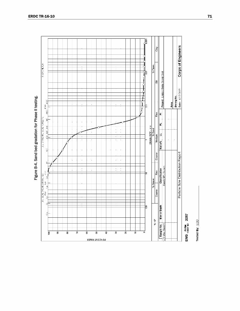
ERDC TR-16-10 71

Figu

re B

-4. S

and

bed

grad

atio

n fo

r Pha

se II

test

ing.

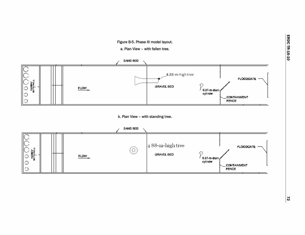
ERD

C TR-16-10

72

Figure B-5. Phase III model layout.

a. Plan View – with fallen tree.

b. Plan View – with standing tree.

ERDC TR-16-10 73

Water depth in the flume was measured at two points inside the flume. The upstream scale was approximately 11.89 m from the metal frame absorbers and anchored into the concrete flume wall. The second down-stream scale was anchored onto the flume wall at approximately 27.43 m downstream of the metal frame absorbers. These two scales were closely monitored throughout testing to ensure that the water level remained constant during testing.

A motor-driven gate at the flume outlet controlled the water level and flow inside the flume. The motors were operated from a control room adjacent to the flume. An overhead video camera was used to monitor the movement of the gate opening during flow setup and to monitor gate status during testing as well as monitor flow depths in the model flume.

A pretest was run to determine the feasibility of running scour tests with both the 0.92-m-diam cylinder placed in the upstream position and the 0.51-m-diam cylinder placed in the downstream position simultaneously. During the pre-test, velocities were measured upstream of the 0.51-m-diam cylinder to assess the effect on flow caused by the 0.92-m-diam cylinder 12.19 m upstream of the 0.51-m-diam cylinder. The velocities were measured at various depths at the centerline of the 0.51-m-diam cylinder and 1.77 m to the left and right of the centerline. Average flow velocity measurements 0.61 m upstream of the 0.51-m-diam cylinder were recorded with a Marsh-McBirney Flo-Mate 2000 portable flow meter© (Figure B-6). Velocities were measured at various depths along the center-line of the flume, directly upstream of the 0.92-m-diam cylinder, with a Vectrino adv velocimeter© (Figure B-7). All six pumps were operating at a flow depth of 0.7 m.

B.1.3 Experiment procedure

A critical velocity, Vc, of 1.44 m/s for the gravel was calculated using the FHWA HEC-18 clear-water scour equation (Richardson and Davis 2001)

/ /c uV K y D

1 6 1 350 (B.1)

where:

Vc = critical velocity above which bed material of size D50 and smaller will be transported (m/s)

y = average depth of flow upstream of the pier (m) D50 = particle size in a mixture of which 50 percent are smaller (m)

ERDC TR-16-10 74

Ku = 6.19 SI units.

Figure B-6. Marsh-McBirney Flo-Mate 2000 portable flow meter©.

Figure B-7. Vectrino adv velocimeter©.

ERDC TR-16-10 75

For comparison to earlier scour testing, an average flow velocity of 0.76 m/s at a water depth of 0.7 m was run during Phase I testing. The 0.76 m/s in the flume, which was 57 percent of the critical velocity of 1.44 m/s, was the maximum velocity achieved in the flume with all six pumps running at a flow depth of 0.7 m. For Phase II testing, water depth remained at 0.7 m, while the average flow velocity was set at 0.35 m/s. This represented approximately 80 percent of the critical velocity, Vc, of 0.44 m/s calculated for the sand using the HEC-18 clear-water scour equation.

To be able to definitively state that scour that occurred around the obstructions was not caused by variations in the starting elevation of the test bed or erosion from the flow at the model inlet, each test began with a completely level test bed. In an effort to ensure that each test started from a point of no known erosion or erosion-causing features in the test bed, the test bed was leveled to grade across the width of the flume by pulling a beam across rails that had been secured to the flume walls at a 1:400 slope.

Once the test bed was leveled to grade, photographs were taken to be processed using photogrammetry software developed at ERDC. The photo-grammetry produced a point cloud that can be measured with Crater Pro© software designed to measure the dimensions of craters created by blasting. Figure B-8 is an example of photographs taken of the pretest bed. The point cloud developed with photogrammetry is shown in Figure B-9.

B.1.4 Experiments and results

B.1.4.1 Phase I

Phase I testing (Table B-1) consisted of four tests with the gravel bed. Tests 1B and 2B were run simultaneously with 0.51-m- and 0.92-m-diam cylinders tall enough to simulate fully obstructed flow, such as would be found with a bridge pier or cylinder. Tests 3B and 4B used the same testing layout but with both cylinders fully submerged 0.33 m and 0.34 m, respectively. A water depth of 0.7 m and a flow of approximately 0.76 m/s was maintained during Phase I testing.

ERDC TR-16-10 76

Figure B-8. Pretest photograph of 0.92-m-diam cylinder.

Figure B-9. Pretest photogrammetry point cloud of 0.92-m-diam cylinder.

Flow

Flow

ERDC TR-16-10 77

Table B-1. Scour study experimental testing matrix.

Phase I. Gravel Bed, Vavg = 0.76 m/s, d = 0.7 m, t = 7.5 hr

Test Test Description Max Scour Depth (cm)

1B Fully obstructed flow – 0.51-m-diam by 0.98-m-high cylinder 27.1


3B Partially obstructed flow – submerged 0.51-m-diam by 0.37-m-high cylinder 18.9

4B Partially obstructed flow – submerged 0.92-m-diam by 0.36-m-high cylinder 25.9

Phase II. Sand Bed, Vavg = 0.35 m/s, d = 0.7 m, t = 7.5 hr


5B Partially obstructed flow - submerged 0.92-m-diam by 0.36-m-high cylinder 17.7


Phase III. Root Ball (tree), Sand Bed, Vavg = 0.35 m/s, d = 0.7 m, t varies


7B Floating tree with 0.84-m-high by 0.97-m-wide root ball facing flow, t = 7.5 hr 13.1

8B Stationary tree with 0.84-m-high by 0.97-m-wide root ball facing flow, t = 7.5 hr 17.4

9Ba Standing tree with root ball on top of sand bed, t = 3 hr 16.2

10B Standing tree with root ball on top of sand bed, t = 7.5 hr 17.1

a Test aborted due to loss of pool after 3 hr of operation.

B.1.4.2 Tests 1B-4B (Phase I)

To minimize scour of the gravel bed at the beginning of each test, the flow was gradually introduced in the upstream headbay. One 0.57-m3/s pump was turned on with a bypass line open and the tailgate closed. As the tail-water depth increased to 0.92 m, the flow was increased by closing the bypass line and adjusting the tailgate to maintain tailwater elevation at 0.92 m. This procedure was repeated as a 1.41-m3/s pump was turned on, alternating additional 0.57- and 1.41-m3/s pumps until all six (three 0.57 m3/s and three 1.41 m3/s) pumps were operating. The tailgate was adjusted until the tailwater elevation stabilized at 0.7 m over the length of the flume for approximately 45 min to 1 hr. Average velocities of 0.76 m/s were measured upstream of the 0.51-m- and 0.92-m-diam cylinders. The model was operated for 7.5 hr.

Upon completion of the testing cycle, the water was slowly lowered in reverse order from startup (i.e., a 1.41-m3/s pump was turned off, then a

ERDC TR-16-10 78

0.57-m3/s pump, alternating until all six pumps were turned off). The flow was monitored to ensure that the scour hole that had formed around the cylinders did not collapse from water rushing out of the test-bed material. Phase I (Table B-1) consisted of tests run simultaneously with the 0.51-m-diam cylinder (Test 1B) and 0.92-m-diam (Test 2B) cylinder rising 0.98 and 0.97 m, respectively, above a gravel bed. The 0.51-m-diam, 0.98-m-high cylinder was located 12.5 m downstream of the 0.92-m-diam, 0.97-m- high cylinder. Flow was fully obstructed by the cylinders rising above the flow. A water depth of 0.7 m and an approximately 0.76 m/s average velocity were maintained during Phase I testing for 7.5 hr. Photographs were taken of the resulting scour and processed using photogrammetry software to obtain a point cloud of data that could then be analyzed in blast analysis software for all tests. The results of the photogrammetry point cloud and analysis software for Test 1B are shown below in Figures B-10 and B-11 and for 2B in Figures B-12 and B-13. Maximum scour occurred at the centerline near the upstream face of the cylinders. Test 1B (0.51-m-diam cylinder with fully obstructed flow) produced a scour hole approximately 27.1 cm deep. Test 2B (0.92-m-diam cylinder with fully obstructed flow) produced a scour hole approximately 38.7 cm deep.

Figure B-10. Test 1B point cloud created using photogrammetry software, 0.51-m-diam cylinder in gravel, fully obstructed flow, Vavg = 0.76 m/s, d = 0.7 m, t = 7.5 hr.

Flow

ERDC TR-16-10 79

Figu

re B

-11.

Ana

lysis

of T

est 1

B us

ing

Crat

er P

ro©

Sof

twar

e 0.

51-m

-dia

m c

ylind

er in

gra

vel,

fully

obs

truct

ed fl

ow, V

avg =

0.7

6 m

/s, d

= 0

.7

m, t

= 7

.5 h

r.

ERDC TR-16-10 80

Figure B-12. Test 2B point cloud created using photogrammetry software, 0.92-m-diam cylinder in gravel, fully obstructed flow, Vavg = 0.76 m/s, d = 0.7 m, t = 7.5 hr.

The heights of the 0.51-m- and 0.92-m-diam cylinders were decreased to 0.37 (Test 3B) and 0.36 m (Test 4B), respectively, above the gravel bed by removing 0.61 m off the top of each cylinder. A water depth of 0.7 m and a flow of approximately 0.76 m/s average velocity were maintained for 7.5 hr. The 0.51-m- and 0.92-m-diam cylinders were submerged 0.33 and 0.34 m, respectively. The results of the photogrammetry point cloud and analysis software for Test 3B are shown below in Figures B-14 and B-15 and for Test 4B inB-16 and B-17. Maximum scour occurred at the centerline near the upstream face of the cylinders. Test 3B (0.51-m-diam cylinder submerged 0.33 m) produced a scour hole approximately 18.9 cm deep. Test 4B (0.92-m-diam cylinder submerged 0.34 m) produced a scour hole approximately 25.9 cm deep.

B.1.4.3 Phase II

Phase II testing (Table B-1) consisted of two separate tests with the 0.92-m-diam cylinder in a 6.09-m-long sand bed. The 0.92-m-diam cylinder extended 0.36 m above the sand bed in Test 5B, simulating a submergence of 0.34 m at a flow depth of 0.7 m and a velocity of 0.35 m/s. The 0.92-m-diam cylinder height was extended above the sand bed by attaching 0.61 m of cylinder to the cylinder from Test 5B. The cylinder extended a total of 0.97 m above the sand bed in Test 6B, simulating a cylinder fully obstructing flow at a flow depth of 0.7 m and a velocity of 0.35 m/s.

Flow

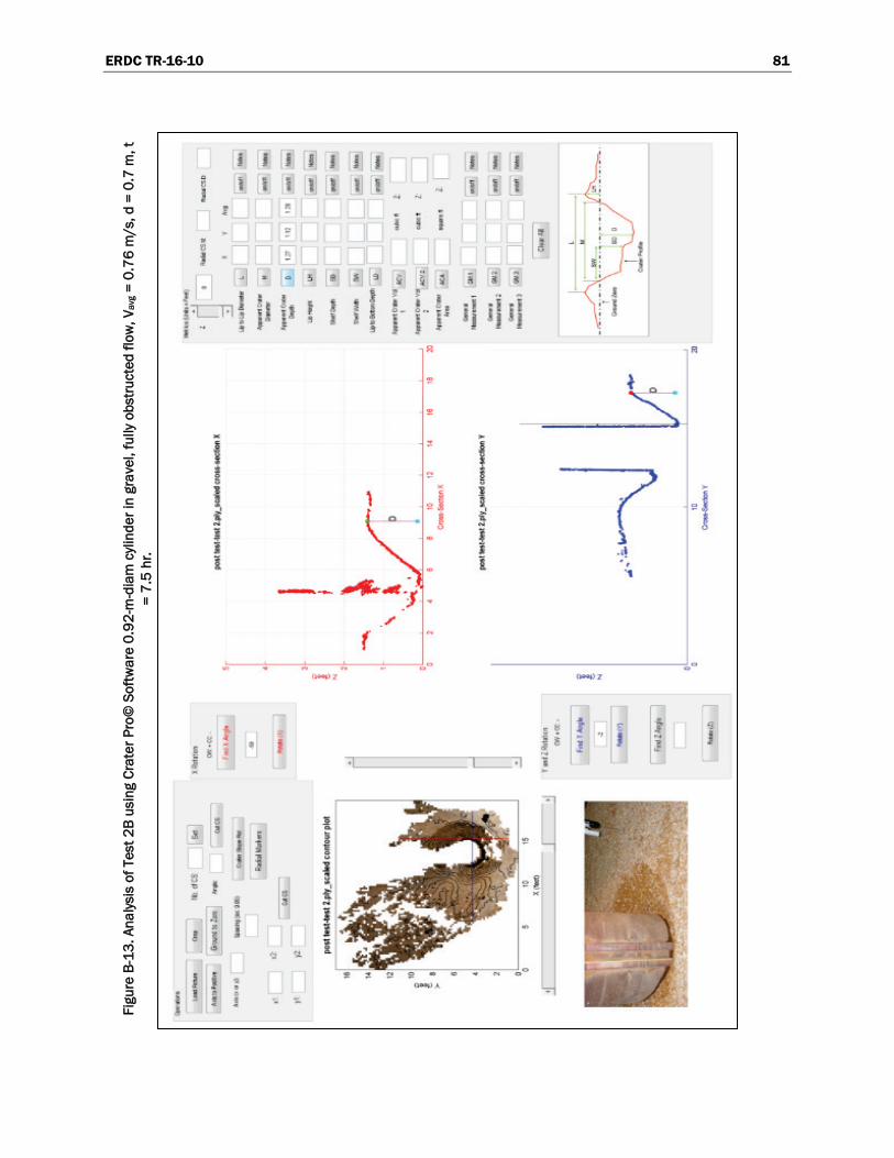
ERDC TR-16-10 81

Figu

re B

-13.

Ana

lysis

of T

est 2

B us

ing

Crat

er P

ro©

Sof

twar

e 0.

92-m

-dia

m c

ylind

er in

gra

vel,

fully

obs

truct

ed fl

ow, V

avg =

0.7

6 m

/s, d

= 0

.7 m

, t

= 7.

5 hr

.

ERDC TR-16-10 82

Figure B-14. Test 3B point cloud created using photogrammetry software, 0.51-m-diam cylinder in gravel, submerged flow, Vavg = 0.76 m/s, d = 0.7 m, t = 7.5 hr.

Flow

ERDC TR-16-10 83

Figu

re B

-15.

Ana

lysis

of T

est 3

B us

ing

Crat

er P

ro©

Sof

twar

e, 0

.51-

m-d

iam

cyli

nder

in g

rave

l, su

bmer

ged

flow

, Vav

g =

0.76

m/s

, d =

0.7

m, t

=

7.5

hr.

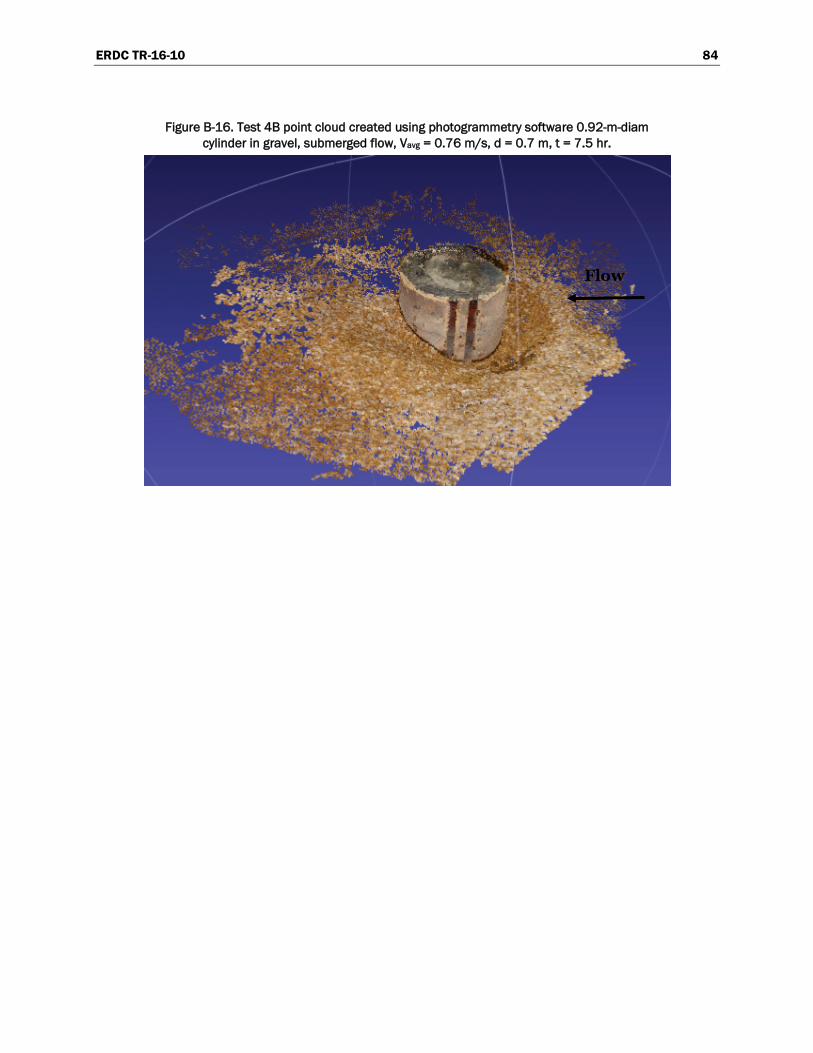
ERDC TR-16-10 84

Figure B-16. Test 4B point cloud created using photogrammetry software 0.92-m-diam cylinder in gravel, submerged flow, Vavg = 0.76 m/s, d = 0.7 m, t = 7.5 hr.

Flow

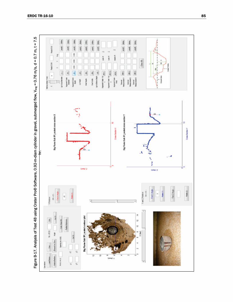
ERDC TR-16-10 85

Figu

re B

-17.

Ana

lysis

of T

est 4

B us

ing

Crat

er P

ro©

Sof

twar

e, 0

.92-

m-d

iam

cyli

nder

in g

rave

l, su

bmer

ged

flow

, Vav

g = 0

.76

m/s

, d =

0.7

m, t

= 7

.5

hr.

ERDC TR-16-10 86

B.1.4.4 Tests 5B-6B (Phase II)

Phase II (Table B-1) consisted of two separate tests with the 0.92-m-diam cylinder in a 6.09-m-long and 1.41-m-deep sand bed test section. The sand bed was constructed around the 0.92-m-diam by 0.36-m-high cylinder. The sand extended 3.05 m upstream and 2.13 m downstream of the cylinder. Time constraints limited the study to the use of only one test section in the flume. Therefore, it was decided to study just the 36-diam cylinder, which produced the greatest scouring effect.

For Tests 5B and 6B, one 0.57-m3/s pump was turned on with a bypass line open and the tailgate closed. As the tailwater depth increased to 0.92 m, the flow was increased by closing the bypass line and adjusting the tailgate to maintain tailwater elevation at 0.92 m. This procedure was repeated as a 1.41-m3/s pump was turned on. The tailgate was adjusted until the tailwater elevation stabilized at 0.7 m over the length of the flume for approximately 45 min to 1 hr. Average velocities of 0.35 m/s were measured upstream of the 0.92-m-diam cylinder. The 0.92-m-diam by 0.36-m-high cylinder was submerged 0.34 m for 7.5 hr of operation (Test 5B). The model flume was gradually drained and photographs for photogrammetry analysis were obtained. The results of the photogrammetry point cloud and analysis software for Test 5B are shown in Figures B-18 and B-19. Maximum scour occurred at the centerline near the upstream face of the cylinder. Test 5B produced a scour hole approximately 17.7 cm deep.

For Test 6B, the 0.92-m-diam cylinder height was extended above the sand bed by attaching 0.61 m of steel to the cylinder from Test 5B. The cylinder extended a total of 0.97 mm above the sand bed, simulating a cylinder fully obstructing flow at a flow depth of 0.7 m and 0.35 m/s average velocity for 7.5 hr. The results of the photogrammetry point cloud and analysis software for Test 6B are shown below in Figures B-20 and B-21. Maximum scour occurred along the centerline near the upstream face of the cylinder. Test 6B produced a scour hole approximately 23.8 cm deep.

B.1.4.5 Phase III

Phase III testing (Table B-1) consisted of four tests with installation of a 4.88-m-tall tree and an intact 0.97-m-wide by 0.84-m-high root ball. The tree trunk diameter increased from 0.27 m, 0.7 m above the sand bed, to 0.67 m at the sand bed. The tree was placed in the sand bed on its side simulating a tree in a fallen position in Tests 7B and 8B. The tree was “stood up” in Tests 9B and 10B, simulating a tree obstructing flow at a flow depth of 0.7 m and 0.35 m/s.

ERDC TR-16-10 87

Figure B-18. Test 5B point cloud created using photogrammetry software, 0.92-m-diam cylinder in sand, submerged flow, Vavg = 0.35 m/s, d = 0.7 m, t = 7.5 hr.

Flow

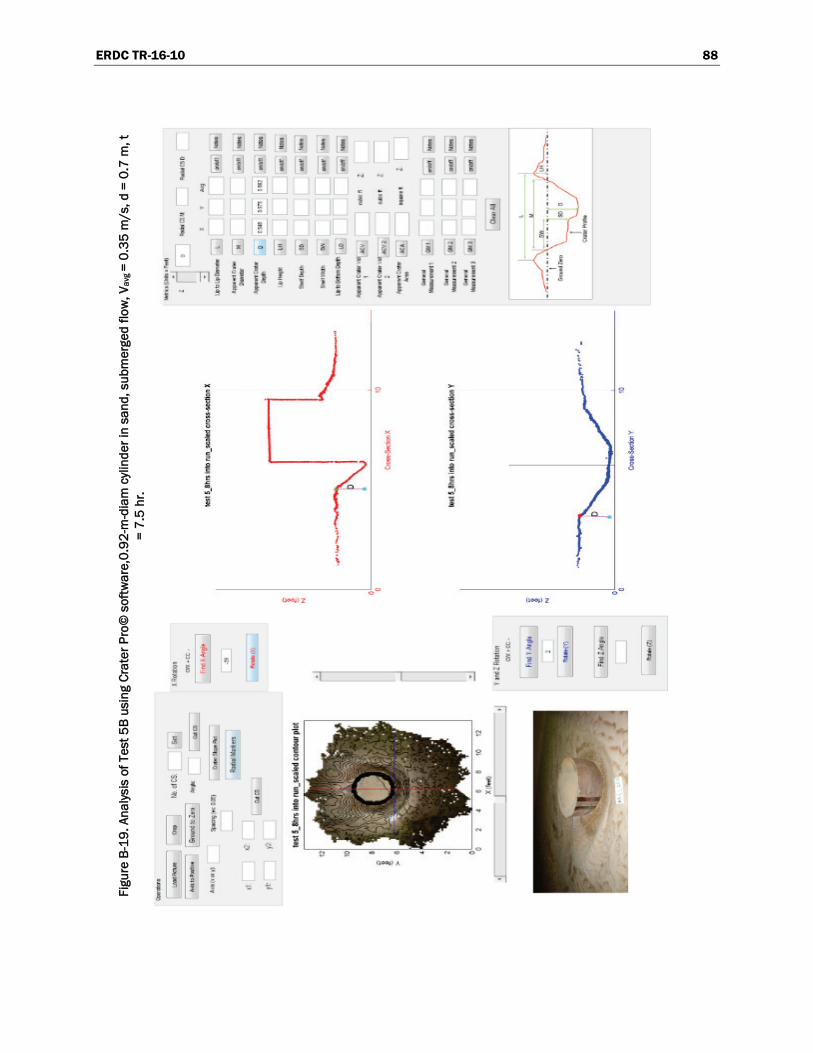
ERDC TR-16-10 88

Figu

re B

-19.

Ana

lysis

of T

est 5

B us

ing

Crat

er P

ro©

sof

twar

e,0.

92-m

-dia

m c

ylind

er in

san

d, s

ubm

erge

d flo

w, V

avg =

0.35

m/s

, d =

0.7

m, t

=

7.5

hr.

ERDC TR-16-10 89

Figure B-20. Test 6B point cloud created using photogrammetry software, 0.92-m-diam cylinder in sand, fully obstructed flow, Vavg = 0.35 m/s, d = 0.7 m, t = 7.5 hr.

Flow

ERDC TR-16-10 90

Figu

re B

-21.

Ana

lysis

of T

est 6

B us

ing

Crat

er P

ro©

sof

twar

e, 0

.92-

diam

cyli

nder

in s

and,

fully

obs

truct

ed fl

ow, V

avg =

0.35

m/s

, d =

0.

7 m

, t =

7.5

hr.

ERDC TR-16-10 91

B.1.4.6 Tests 7B-10B (Phase III)

Phase III tests (Table B-1) consisted of a tree in the 6.1-m-long sand test bed. A 4.88-m-high tree with an intact 0.97-m-wide by 0.84-m-high root ball replaced the 0.92-m-diam cylinder. The test procedure from Test 5B was repeated with the tree in the fallen position with its root ball facing upstream (Tests 7B and 8B). The tree was allowed to float for 7.5 hr (Test 7B). The model flume was gradually drained and photographs for photogrammetry analysis were recorded. The results of the photogram-metry point cloud and analysis software for Test 7B are shown below in Figures B-22 and B-23. Test 7B produced a scour hole approximately 13.1 cm deep on the right side of the tree looking downstream.

With the tree in the fallen position, the model bed was remolded and the tree was physically restrained using weights and braces to prevent it from floating for 7.5 hr (Test 8B). The model flume was gradually drained and photographs for photogrammetry analysis were recorded. The results of the photogrammetry point cloud and analysis software for Test 8B are shown below in Figures B-24 and B-25. Test 8B produced a scour hole approximately 17.4 cm deep on the right side of the tree looking downstream.

The 4.88-m-high tree with an intact 0.97-m-wide by 0.84-m-high root ball was placed in a vertical position on a 3.05-m-wide by 0.92-m-diam plastic barrel to simulate a pine tree with a tap root (Figure B-26). The test procedure from Test 7B was repeated with the tree standing in the model (Tests 9B and 10B). During Test 9B, the pool remained steady for 3 hr. The test was aborted after loss of pool at 3 hr of operation. The model flume was gradually drained and photos for photogrammetry analysis were recorded. The results of the photogrammetry point cloud and analysis software for Test 9B are shown below in Figures B-27 and B-28. Test 9B produced a scour hole approximately 16.2 cm deep on the right side of the tree looking downstream.

The model sand bed was remolded to grade. Flow was introduced again using one 0.57-m3/s and one 1.41-m3/s pump. Once flow stabilized at 0.7 m of depth and 0.35 m/s, the model was operated for 7.5 hr (Test 10B).

ERDC TR-16-10 92

Figure B-22. Test 7B point cloud created using photogrammetry software, tree in fallen position in sand, tree floating, Vavg = 0.35 m/s, d = 0.7 m, t = 7.5 hr.

Flow

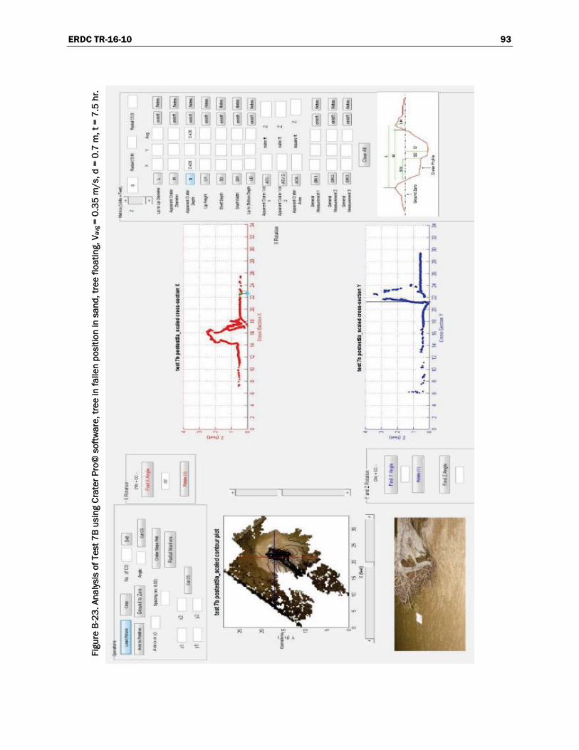
ERDC TR-16-10 93

Figu

re B

-23.

Ana

lysis

of T

est 7

B us

ing

Crat

er P

ro©

sof

twar

e, tr

ee in

falle

n po

sitio

n in

san

d, tr

ee fl

oatin

g, V

avg =

0.35

m/s

, d =

0.7

m, t

= 7

.5 h

r.

ERDC TR-16-10 94

Figure B-24. Test 8B point cloud created using photogrammetry software, tree in fallen position in sand, tree stationary, Vavg = 0.35 m/s, d = 0.7 m, t = 7.5 hr.

Flow

ERDC TR-16-10 95

Figu

re B

-25.

Ana

lysis

of T

est 8

B us

ing

Crat

er P

ro©

sof

twar

e, tr

ee in

falle

n po

sitio

n in

san

d, tr

ee s

tatio

nary

, Vav

g =

0.35

m/s

, d =

0.7

m, t

= 7

.5

hr.

ERDC TR-16-10 96

Figure B-26. Standing tree in flume on blue barrel.

Figure B-27. Test 9B, tree in vertical position in sand, fully obstructed flow, Vavg = 0.35 m/s, d = 0.7 m, t = 3 hr.

The model flume was gradually drained and photographs for photo-grammetry analysis were recorded. The results of the photogrammetry point cloud and analysis software for Test 10B are shown below in Figures B-29 and B-30. Test 10B produced a scour hole approximately 17.1 cm deep on the right side of the tree looking downstream.

Flow

ERDC TR-16-10 97

Figure B-28. Test 9B point cloud created using photogrammetry software, tree in vertical position in sand, fully obstructed flow, Vavg = 0.35 m/s, d = 0.7 m, t = 3 hr.

Flow

ERDC TR-16-10 98

Figu

re B

-29.

Ana

lysis

of T

est 9

B us

ing

Crat

er P

ro©

sof

twar

e, tr

ee in

ver

tical

pos

ition

in s

and,

fully

obs

truct

ed fl

ow, V

avg =

0.35

m/s

, d =

0.7

m, t

= 3

hr

.

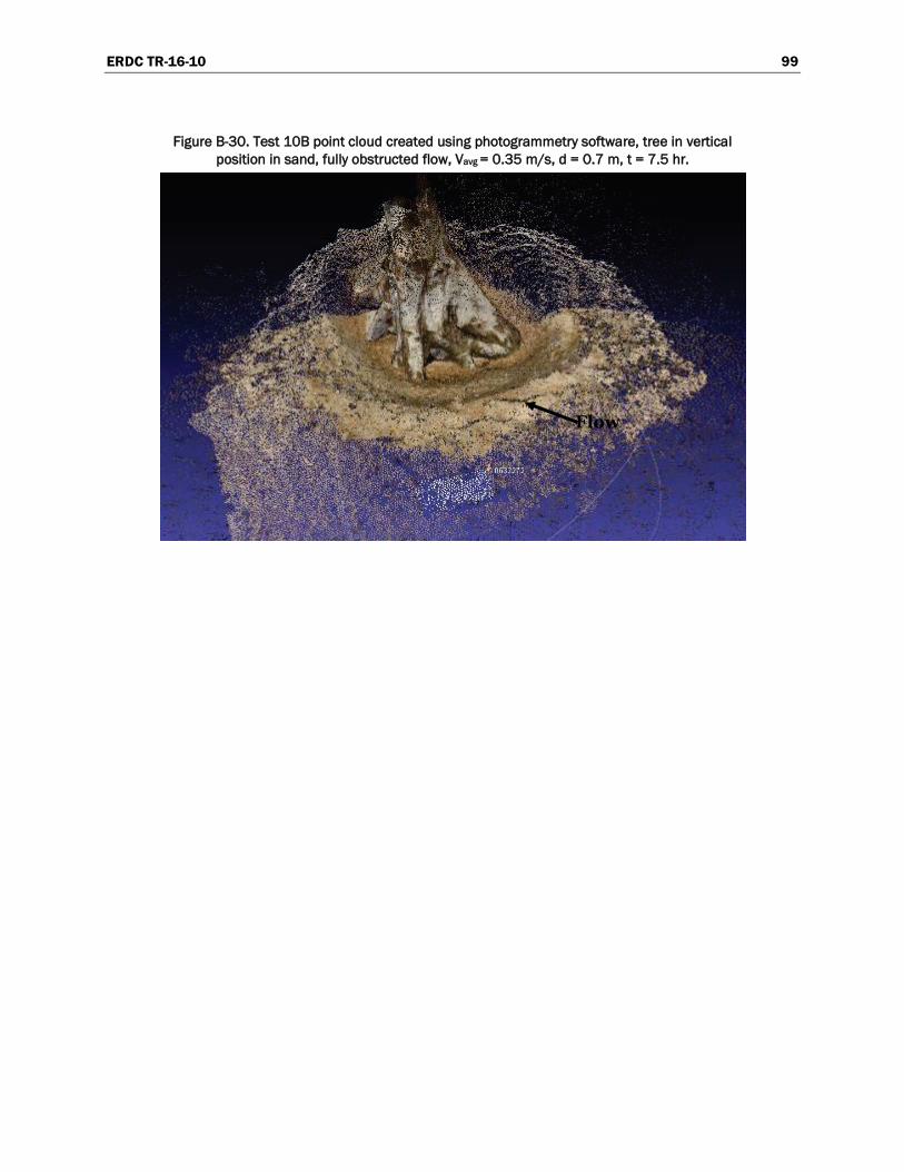
ERDC TR-16-10 99

Figure B-30. Test 10B point cloud created using photogrammetry software, tree in vertical position in sand, fully obstructed flow, Vavg = 0.35 m/s, d = 0.7 m, t = 7.5 hr.

Flow

ERDC TR-16-10 100

Figu

re B

-31.

Ana

lysis

of T

est 1

0B u

sing

Cra

ter P

ro©

sof

twar

e, tr

ee in

ver

tical

pos

ition

in s

and,

fully

obs

truct

ed fl

ow, V

avg =

0.35

m/s

, d =

0.7

m, t

= 7

.5

hr.

ERDC TR-16-10 101

Results

For comparison to earlier scour testing, an average flow velocity of 0.76 m/s at a water depth of 0.7 m was run during Phase I testing. A criti-cal velocity, Vc, of 1.44 m/s for the gravel was calculated using the FHWA, HEC-18 clear-water scour equation (Richardson and Davis 2001)

/ /c uV K y D 1 6 1 3

50

where:

Vc = critical velocity above which bed material of size D50 and smaller will be transported (m/s)

y = average depth of flow upstream of the pier (m) D50 = particle size in a mixture of which 50 percent are smaller (m) Ku = 6.19 SI units.

The 0.76 m/s in the flume, which was 57 percent of the critical velocity of 1.44 m/s for clear scour for the gravel in the flume with a D50 of 1.43 mm, was the maximum velocity achieved in the flume with all six pumps run-ning at a flow depth of 0.7 m. The results of the tests tabulated in Table B-1 indicated that scour depth was greater upstream of the 0.92-m-diam cylindrical obstruction than the scour depth upstream of the 0.51-m cylindrical obstruction for each flow condition. The scour depth was greatest when flow depth was fully obstructed for the 0.92-m and 0.51-m cylindrical obstructions in gravel. Tests conducted at 50 percent submer-gence of the cylindrical obstruction in gravel produced less scour than the scour produced with fully obstructed flow. The resulting scour in the flume was less than the scour predicted by the Sheppard-Melville bridge pier equations. The difference between the model scour depth and the Sheppard-Melville predicted scour depth may be attributed to several factors: (a) the average velocity in the gravel model was 57 percent of the clear-water critical velocity, resulting in lower scour depth, (b) the clear-water contraction scour equations assume homogeneous bed materials and the material in the gravel model were not homogeneous, and (c) the gravel produced armoring of the scour hole, reducing the depth of scour in the model.

Water depth remained at 0.7 m, while the average flow velocity was reduced to 0.35 m/s for fully obstructed and submerged flow around the 0.92- and

ERDC TR-16-10 102

0.51-m cylinders in coarse sand (Phase II tests). The velocity of 0.35 m/s represented approximately 80 percent of the critical velocity of 0.44 m/s for clear scour of the sand in the flume with a D50 of 0.43 mm. The results of the Phase II tests tabulated in Table B-1 indicated that scour depth was greater upstream of the 0.92-m-diam cylindrical obstruction with fully obstructed flow than upstream of the 0.92-m cylindrical obstruction submerged 50 percent. The resulting scour in the flume was less than the scour predicted by the Sheppard-Melville bridge pier equations. The difference between the model scour depth and the Sheppard-Melville predicted scour depth may be attributed to several factors: (a) the average velocity in the sand model was 80 percent of the clear-water critical velocity resulting in lower scour depth, (b) the clear-water contraction scour equa-tions assume homogeneous bed materials and the material in the sand model were coarsely graded, and (c) the gravel and pebbles in the coarse sand produced armoring of the scour hole, reducing the depth of scour in the model. Further investigation is recommended for this situation.

The water depth remained at 0.7 m and the average flow velocity was 0.35 m/s for the Phase III tests with the tree in the sand test bed. The results of the Phase III tests tabulated in Table B-1 indicated that scour depth resulting from the tree in both the fallen and vertical positions was approximately equal to the scour depth resulting from the 0.92-m cylinder fully obstructing flow in the sand test bed. The scour was deepest on the right side of the tree looking downstream. The asymmetric geometry of the root structure and the semi-porous nature of the root wad most likely contributed to the development of deeper scour on the right side of the tree looking downstream. The difference between the model scour depth and the Sheppard-Melville predicted scour depth may be attributed to several factors: (a) the average velocity in the sand model was 80 percent of the clear-water critical velocity, resulting in lower scour depth; (b) the clear-water contraction scour equations assume homogeneous bed materials and the material in the sand model were coarsely graded; (c) the gravel and pebbles in the coarse sand produced armoring of the scour hole, reducing the depth of scour in the model; (d) the asymmetrical geometry of the tree root wad in the fallen position as well as in the vertical position was different from the symmetrical cylinders used to calculate scour in the Sheppard-Melville bridge pier scour equation; (e) the roughness of the irregular root ball surface might have introduced turbulence that prevented the downward plunging jet from fully forming; and (f) as material was washed away from the root ball, the “obstruction” became more porous and flow passed through the root ball instead of being deflected by it.

REPORT DOCUMENTATION PAGE Form Approved

OMB No. 0704-0188 Public reporting burden for this collection of information is estimated to average 1 hour per response, including the time for reviewing instructions, searching existing data sources, gathering and maintaining the data needed, and completing and reviewing this collection of information. Send comments regarding this burden estimate or any other aspect of this collection of information, including suggestions for reducing this burden to Department of Defense, Washington Headquarters Services, Directorate for Information Operations and Reports (0704-0188), 1215 Jefferson Davis Highway, Suite 1204, Arlington, VA 22202-4302. Respondents should be aware that notwithstanding any other provision of law, no person shall be subject to any penalty for failing to comply with a collection of information if it does not display a currently valid OMB control number. PLEASE DO NOT RETURN YOUR FORM TO THE ABOVE ADDRESS. 1. REPORT DATE (DD-MM-YYYY)

July 2016 2. REPORT TYPE

Final 3. DATES COVERED (From - To)

4. TITLE AND SUBTITLE


5a. CONTRACT NUMBER

5b. GRANT NUMBER

5c. PROGRAM ELEMENT NUMBER 031398

6. AUTHOR(S)

Deborah R. Cooper, Charles D. Little, Jr., Julie Cohen, Brendan Yuill, Johannes Wibowo, Bryant Robbins, Raymond Reed, Maureen K. Corcoran, and Kevin S. Holden

5d. PROJECT NUMBER 454633

5e. TASK NUMBER A1200

5f. WORK UNIT NUMBER

7. PERFORMING ORGANIZATION NAME(S) AND ADDRESS(ES) 8. PERFORMING ORGANIZATION REPORT NUMBER

Geotechnical and Structures Laboratory U.S. Army Engineer Research and Development Center 3909 Halls Ferry Road Vicksburg, MS 39180-6199

ERDC TR-16-10

9. SPONSORING / MONITORING AGENCY NAME(S) AND ADDRESS(ES) 10. SPONSOR/MONITOR’S ACRONYM(S) Headquarters, U.S. Army Corps of Engineers Washington, DC 20314-1000

HQ-USACE 11. SPONSOR/MONITOR’S REPORT NUMBER(S)

12. DISTRIBUTION / AVAILABILITY STATEMENT Approved for public release; distribution is unlimited.

13. SUPPLEMENTARY NOTES

14. ABSTRACT Existing bridge pier scour prediction equations exclude the influence of tree roots and the cross slope of levee embankments. Developed for specific conditions, these equations do not include modeling of scour at trees near or on levee embankments. Therefore, existing bridge pier scour models must be carefully evaluated and possibly modified before being applied to tree scour.

The research conducted by the U.S. Army Engineer Research and Development Center (ERDC) included review and evaluation of the Sheppard-Melville and the Federal Highway Administration Hydraulic Engineering Circular No. 18 (FHWA HEC-18) bridge pier scour equations and validation flume experiments. The research objective was to provide guidance for predicting maximum scour depths near trees on or near levee embankments. The Sheppard-Melville and the HEC-18 methods of bridge pier scour prediction were evaluated. Results from the flume experiments indicate that both methods consistently over-predict scour depth by as much as 25 to 75 percent. Although other bridge scour equations can be used, both the Sheppard-Melville and the HEC-18 equations are sufficient in assessing tree scour potential to conservatively estimate maximum scour that may occur.

. 15. SUBJECT TERMS (see reverse)

16. SECURITY CLASSIFICATION OF: 17. LIMITATION OF ABSTRACT

18. NUMBER OF PAGES

19a. NAME OF RESPONSIBLE PERSON

a. REPORT

Unclassified

b. ABSTRACT

Unclassified

c. THIS PAGE

Unclassified Unclassified 114 19b. TELEPHONE NUMBER (include area code)

Standard Form 298 (Rev. 8-98) Prescribed by ANSI Std. 239.18

15. SUBJECT TERMS (concluded) Bridge scour equations Scour around trees Sheppard-Melville method Woody vegetation Bridges-Foundations & piers Scour (Hydraulic engineering) Roots (Botany) Trees Levees Embankments Numerical analysis

Documents

· The research conducted by the U.S. Army Engineer Research and Development Center (ERDC) included review and evaluation of the Sheppard-Melville and the Federal Highway Administrat