GLOBCOLOUR · The GlobColour primary data set has now been delivered as a Group on Earth Observations ... LOV Laboratoire Océanologique de Villefranche-sur-mer

GlobColour

Product User Guide

Ref: GC-UM-ACR-PUG-01

Date : 31/08/2017

Issue : version 4.1

Page : 1

GLOBCOLOUR

Product User’s Guide

Reference: GC-UM-ACR-PUG-01

Version 4.1

August 2017

GlobColour

Product User Guide


Date : 31/08/2017

Issue : version 4.1

Page : 2

Document Signature Table

Name Function Company Signature Date

Author ACRI-ST GlobColour Team

ACRI-ST

Verification A. Mangin Scientific Director

ACRI-ST

Approval O. Fanton d’Andon President ACRI-ST

Change record

Issue Date Change Log

1.0 17/11/2006 Product User Guide

1.1 22/12/2006 Updated pages



2.0 08/01/2010 New parameters have been added (to be compliant with MKL3 outputs)

3.0 draft 27/10/2014 GlobColour 2nd reprocessing (draft version)

3.0 05/12/2014 GlobColour 2nd reprocessing

3.1 13/02/2015 Corrected ftp address

3.2 19/10/2015 Update VIIRS to R2014.0 (including new error bars)

4.0 19/11/2015

10/06/2016

14/11/2016

02/03/2017

Update production delivery time

Update SeaWiFS to R2014.0 (including new error bars)

Update MODIS to R2014.0

Add CHL-OC5, SPM-OC5 and KDPAR-SAULQUIN

4.1 31/08/2017 Add OLCI sensor

GlobColour

Product User Guide


Date : 31/08/2017

Issue : version 4.1

Page : 3

GlobColour

Product User Guide


Date : 31/08/2017

Issue : version 4.1

Page : 4

Table of content

1 INTRODUCTION .............................................................................................................8

1.1 Background ..............................................................................................................8 1.2 Scope of the document.............................................................................................8 1.3 Acronyms .................................................................................................................9 1.4 Brief overview of GlobColour products ...................................................................10

1.4.1 Parameters .....................................................................................................10 1.4.2 Spatial Domain ................................................................................................11 1.4.3 Sensors ...........................................................................................................12 1.4.4 Spatial and Temporal resolutions ....................................................................12

2 THE PRODUCTS CONTENT ........................................................................................13

2.1 Parameters overview ..............................................................................................13 2.1.1 Biological parameters ......................................................................................14 2.1.2 Atmospheric Optical parameters .....................................................................14 2.1.3 Ocean Surface Optical parameters .................................................................15 2.1.4 Ocean Subsurface Optical parameters ............................................................16 2.1.5 OSS2015 Demonstration Biological Products..................................................17

2.2 Parameter Detailed Description ..............................................................................17 2.2.1 CHL1 ...............................................................................................................18 2.2.2 CHL-OC5 ........................................................................................................20 2.2.3 SPM-OC5 ........................................................................................................21 2.2.4 CHL2 ...............................................................................................................22 2.2.5 TSM ................................................................................................................23 2.2.6 PIC ..................................................................................................................24 2.2.7 POC ................................................................................................................25 2.2.8 NFLH ..............................................................................................................26 2.2.9 WVCS .............................................................................................................27 2.2.10 Txxx ................................................................................................................28 2.2.11 Axxx ................................................................................................................30 2.2.12 CF ...................................................................................................................32 2.2.13 ABSD ..............................................................................................................33 2.2.14 (N)RRSxxx ......................................................................................................34 2.2.15 EL555 .............................................................................................................37 2.2.16 PAR ................................................................................................................38 2.2.17 BBP .................................................................................................................39 2.2.18 CDM ................................................................................................................40 2.2.19 KD490 .............................................................................................................42 2.2.20 KDPAR............................................................................................................45 2.2.21 ZHL .................................................................................................................47 2.2.22 ZEU .................................................................................................................48 2.2.23 ZSD .................................................................................................................49 2.2.24 CHL-CIA ..........................................................................................................51 2.2.25 BBPxxx-LOG ...................................................................................................52 2.2.26 BBPS-LOG ......................................................................................................53 2.2.27 PSD-XXX ........................................................................................................54 2.2.28 POC-SURF .....................................................................................................55

GlobColour

Product User Guide


Date : 31/08/2017

Issue : version 4.1

Page : 5

2.2.29 POC-INT .........................................................................................................56 2.2.30 PP-AM, PP-UITZ .............................................................................................57 2.2.31 PHYSAT ..........................................................................................................59

2.3 The spatial and temporal coverage ........................................................................60 2.3.1 The binned products........................................................................................60 2.3.2 The mapped products .....................................................................................60

3 THE GLOBCOLOUR SYSTEM .....................................................................................61

3.1 Overall description of the processor .......................................................................61 3.2 The preprocessor ...................................................................................................63

3.2.1 MERIS.............................................................................................................64 3.2.2 OLCI ...............................................................................................................66 3.2.3 MODIS/SeaWiFS/VIIRS ..................................................................................67

3.3 The spatial and temporal binning schemes.............................................................67 3.4 The GlobColour data-day approach........................................................................68

4 THE PRODUCTS FORMAT ..........................................................................................73

4.1 General rules ..........................................................................................................73 4.2 Naming convention .................................................................................................73 4.3 The binned products ...............................................................................................74 4.4 The mapped products ............................................................................................80

5 HOW TO…? ..................................................................................................................82

5.1 Access the GlobColour data ...................................................................................82 5.1.1 The HERMES interface ...................................................................................82 5.1.2 Ordering GlobColour Products ........................................................................83 5.1.3 Ordering OSS2015 demonstration products ....................................................86 5.1.4 Ordering a list of products ...............................................................................87 5.1.5 Retrieving the data ..........................................................................................87

5.2 Download the data from the GlobColour ftp server .................................................88 5.3 Read the data .........................................................................................................88 5.4 Visualize the data ...................................................................................................89

6 APPENDICES ...............................................................................................................92

6.1 Global ISIN grid definition .......................................................................................92 6.2 Summary of products content .................................................................................93 6.3 The main characteristics of the products ................................................................94 6.4 The steps of the binning and merging schemes .....................................................95

6.4.1 Step 1: L2 to L3 track ......................................................................................95 6.4.2 Step 2: L3 track to L3 daily for each single instrument .....................................96 6.4.3 Step 3: L3 daily for each single instrument to merged L3 daily ........................97 6.4.4 Step 4: L3 daily merged to 8-days and monthly L3 ..........................................98 6.4.5 Step 5: L3 daily/8days/monthly merged products to mapped products ............98 6.4.6 Step 6: generation of the quicklooks ................................................................99

6.5 The error bars ........................................................................................................99 6.6 Common Data Language description ................................................................... 100 6.7 References ........................................................................................................... 103

6.7.1 GlobColour products references .................................................................... 103 6.7.2 References for OSS2015 demonstration products ........................................ 105

GlobColour

Product User Guide


Date : 31/08/2017

Issue : version 4.1

Page : 6

List of Tables

Table 1-1: Available sensors in the GlobColour data set ......................................................12

Table 1-2: Overview of the GlobColour products ..................................................................12

Table 2-1: List of GlobColour Biological Parameters.............................................................14

Table 2-2: List of GlobColour Atmospheric Optical parameters ............................................14

Table 2-3: List of GlobColour Ocean Surface Optical parameters.........................................15

Table 2-4: GlobColour Ocean Subsurface parameters .........................................................16

Table 2-5: Main characteristics of the ISIN grids ...................................................................60

Table 3-1: List of variables with a specific preprocessing .....................................................63

Table 3-2: List of parameters and filters applied to the MERIS level 2 data ..........................65

Table 3-3: List of parameters and filters applied to the OLCI level 2 data .............................66

Table 3-4: List of parameters and filters applied to the MODIS/SeaWiFS/VIIRS level 2 data 67

Table 3-5: Input parameters for data-day classification .........................................................71

Table 3-6: CNT of satellites ..................................................................................................72

Table 4-1: Dimensions - binned products .............................................................................75

Table 4-2: Variables - binned products .................................................................................75

Table 4-3: Flags description .................................................................................................76

Table 4-4: Variables attributes - binned products ..................................................................77

Table 4-5: Global attributes - binned products (1/3) ..............................................................78



Table 4-8: Dimensions of the grid - mapped products...........................................................80

Table 4-9: Dimensions - mapped products ...........................................................................81

Table 4-10: Variables - mapped products (1/2) .....................................................................81

Table 4-11: Variables - mapped products (2/2) .....................................................................81

Table 6-1: ISIN grid definition ...............................................................................................92

Table 6-2: Summary of products content ..............................................................................93

Table 6-3: Error Bars used to generate Weighted Average products ....................................99

GlobColour

Product User Guide


Date : 31/08/2017

Issue : version 4.1

Page : 7

List of Figures

Figure 1-1: A sample GlobColour Global product .................................................................11

Figure 1-2: A sample GlobColour Europe product ................................................................11

Figure 3-1: The GlobColour processor high-level description ...............................................62

Figure 3-2: MERIS pixels UTC as a function of the pixel longitude (35 days - October 2003) ......................................................................................................................................69

Figure 3-3: MODIS pixels UTC as a function of the pixel longitude (1 day - June 2003) .......69

Figure 3-4:SeaWiFS pixels UTC as a function of the pixel longitude (1 day - December 2003) ......................................................................................................................................70

Figure 3-5: Data-day definition line above MODIS pixels UTC versus longitude plot. ...........70

Figure 3-6: Data-day definition line above one SeaWiFS track. ............................................71

Figure 5-1: the HERMES Interface .......................................................................................82

Figure 5-2: GlobColour Data Access interface ......................................................................83

Figure 5-3: Selection of the map overlays .............................................................................84

Figure 5-4: Selected products list and previsualisation screen ..............................................86

Figure 5-5: OS2015 products data access ............................................................................87

Figure 5-6: Visualization of a GlobColour L3m product using Visat.......................................89

Figure 5-7: Visualization of a GlobColour L3m product using ncview. ...................................89

Figure 5-8: Visualizing GlobColour products with matplotlib .................................................90

Figure 5-9: Generated image ................................................................................................91

GlobColour

Product User Guide


Date : 31/08/2017

Issue : version 4.1

Page : 8

1 Introduction

1.1 Background

The GlobColour project started in 2005 as an ESA Data User Element (DUE) project to provide a continuous data set of merged L3 Ocean Colour products. Merging outputs from different sensors ensures data continuity, improves spatial and temporal coverage and reduces data noise. This allows in particular to process long time series of consistent products (trend analysis, climatology, data assimilation for model hindcast).

Since then, ACRI has maintained the archive and Near Real Time data access services through the Hermes website.

The 2014 reprocessing and the update of the Hermes interface were performed in the framework of the OSS2015 project, with funding from the EU FP7 under grant n°282723.

The GlobColour project has received additional funding from European Union FP7 under grant agreement n° 218812 (MyOcean) and from PACA Region under project RegiColour.

From May 2015, the GlobColour project also contributes to the Copernicus Marine Environment Monitoring Service (CMEMS). A subset of the GlobColour products is disseminated by CMEMS. It concerns at present Chlorophyll, reflectances, Secchi depth, SPM, BBP, KD490 merged products (Near Real Time and the long time series).

In addition, support from NASA regarding access to L2 products is acknowledged.

The GlobColour primary data set has now been delivered as a Group on Earth Observations System of Systems (GEOSS) core data set under reference:

urn:geoss:csr:resource:urn:uuid:4e33fd81-d5cc-dc40-b645-ab961447d9d8.

1.2 Scope of the document

This User Guide contains a description of:

the products content

- the parameters

- the spatial and temporal coverage

- the processing system

the products format

Hermes interface user’s guide

Appendices containing additional information on products and processing

http://www.myocean.eu.org/

http://marine.copernicus.eu/

http://www.earthobservations.org/geoss.php

GlobColour

Product User Guide


Date : 31/08/2017

Issue : version 4.1

Page : 9

1.3 Acronyms

AV Simple average method

AVW Weighted average method

bbp Particulate back-scattering coefficient

BEAM Basic ERS and Envisat (A)ATSR and MERIS Toolbox

BOUSSOLE Bouée pour l’acquisition de Séries Optiques à Long Terme

CDL Common Data Language

CDM Coloured dissolved and detrital organic materials absorption coefficient

CF Climate and Forecast

CF Cloud Fraction

CHL Chlorophyll-a

CZCS Coastal Zone Color Scanner

DLR Deutsches Zentrum für Luft- und Raumfahrt

DPM Detailed Processing Model

DUE Data User Element of the ESA Earth Observation Envelope Programme II

EEA European Environment Agency

EL555 Relative excess of radiance at 555 nm (%)

EO Earth observation

GHRSST-PP GODAE High Resolution Sea Surface Temperature - Pilot Project

GSM Garver, Siegel, Maritorena Model

ICESS Institute for Computational and Earth Systems Science

IOCCG International Ocean Colour Coordinating Group

IOCCP International Ocean Carbon Coordination Project

IODD Input Output Data Definition

ISIN Integerised SINusoidal projection

LOV Laboratoire Océanologique de Villefranche-sur-mer

LUT Look-Up Table

MER Acronym for the MERIS instrument used in the GlobColour filenames

MERIS Medium Resolution Imaging Spectrometer

MERSEA Marine Environment and Security for the European Area –

Integrated Project of the EC Framework Programme 6

MOBY Marine Optical Buoy

MOD Acronym for the MODIS instrument used in the GlobColour filenames

MODIS Moderate Resolution Imaging Spectrometer

netCDF Network Common Data Format

NIVA Norwegian Institute for Water Research

(N)RRSXXX Fully normalised remote sensing reflectances at xxx nm (sr-1)

NRT Near-real time

OLCI Ocean Land Colour Instrument

GlobColour

Product User Guide


Date : 31/08/2017

Issue : version 4.1

Page : 10

PAR Photosynthetic Available Radiation

PC Plate-Carré projection

PNG Portable Network Graphics

RD Reference Document

ROI / RoI Region of Interest

SeaBASS SeaWiFS Bio-Optical Archive and Storage System

SeaWiFS Sea-Viewing Wide Field of View Sensor

SAA Sun Azimuth Angle

SWF Acronym for the SeaWiFS instrument used in the GlobColour filenames

SZA Sun Zenith Angle

TSM Total Suspended Matter

T865 Aerosol optical thickness over water

UCAR University Corporation for Atmospheric Research

UoP University of Plymouth (U.K)

UTC Coordinated Universal Time

VAA Viewing Azimuth Angle

VZA Viewing Zenith Angle

1.4 Brief overview of GlobColour products

1.4.1 Parameters

The parameters of the GlobColour data set are:

Biological parameters: Chlorophyll (several algorithms), Particulate Organic/Inorganic Carbon, Fluorescence…

Atmosphere optical parameters: aerosol thickness, cloud fraction, water vapour column…

Ocean-surface optical parameters: reflectances

Sub-surface optical parameters: attenuation and back-scattering coefficients, turbidity

The full list of parameters is provided in section 2.1.

For some parameters, several alternative algorithms are proposed. This is the case when no algorithm is clearly superior to the other(s). The relative performance may vary depending on the conditions (water types, regions, sensors…), and users are advised to compare the results on a case-by-case basis.

GlobColour

Product User Guide


Date : 31/08/2017

Issue : version 4.1

Page : 11

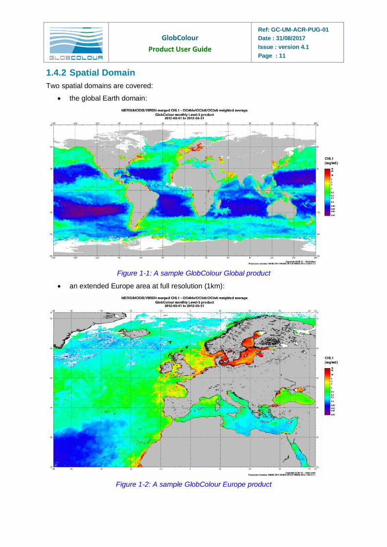
1.4.2 Spatial Domain

Two spatial domains are covered:

the global Earth domain:

Figure 1-1: A sample GlobColour Global product

an extended Europe area at full resolution (1km):

Figure 1-2: A sample GlobColour Europe product

GlobColour

Product User Guide


Date : 31/08/2017

Issue : version 4.1

Page : 12

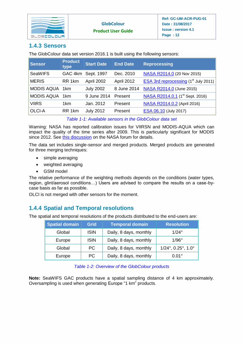
1.4.3 Sensors

The GlobColour data set version 2016.1 is built using the following sensors:

Sensor Product type

Start Date End Date Reprocessing

SeaWIFS GAC 4km Sept. 1997 Dec. 2010 NASA R2014.0 (20 Nov 2015)

MERIS RR 1km April 2002 April 2012 ESA 3rd reprocessing (1st July 2011)

MODIS AQUA 1km July 2002 8 June 2014 NASA R2014.0 (June 2015)

MODIS AQUA 1km 9 June 2014 Present NASA R2014.0.1 (1st Sept. 2016)

VIIRS 1km Jan. 2012 Present NASA R2014.0.2 (April 2016)

OLCI-A RR 1km July 2012 Present ESA 06.10 (July 2017)

Table 1-1: Available sensors in the GlobColour data set

Warning: NASA has reported calibration issues for VIIRSN and MODIS-AQUA which can impact the quality of the time series after 2009. This is particularly significant for MODIS since 2012. See this discussion on the NASA forum for details.

The data set includes single-sensor and merged products. Merged products are generated for three merging techniques:

simple averaging

weighted averaging

GSM model

The relative performance of the weighting methods depends on the conditions (water types, region, glint/aerosol conditions…) Users are advised to compare the results on a case-by-case basis as far as possible.

OLCI is not merged with other sensors for the moment.

1.4.4 Spatial and Temporal resolutions

The spatial and temporal resolutions of the products distributed to the end-users are:

Spatial domain Grid Temporal domain Resolution

Global ISIN Daily, 8 days, monthly 1/24°

Europe ISIN Daily, 8 days, monthly 1/96°

Global PC Daily, 8 days, monthly 1/24°, 0.25°, 1.0°

Europe PC Daily, 8 days, monthly 0.01°

Table 1-2: Overview of the GlobColour products

Note: SeaWIFS GAC products have a spatial sampling distance of 4 km approximately. Oversampling is used when generating Europe “1 km” products.

https://oceancolor.gsfc.nasa.gov/reprocessing/r2014/seawifs

https://earth.esa.int/web/guest/missions/esa-operational-eo-missions/envisat/news/-/asset_publisher/x9cY/content/meris-reduced-resolution-3rd-reprocessing-dataset-now-opened-to-users-7741

https://oceancolor.gsfc.nasa.gov/reprocessing/r2014/aqua

https://oceancolor.gsfc.nasa.gov/reprocessing/r2014/aqua#R2014.0.1

https://oceancolor.gsfc.nasa.gov/reprocessing/r2014/viirs-snpp

http://www.eumetsat.int/website/wcm/idc/idcplg?IdcService=GET_FILE&dDocName=PDF_S3A_PN_OLCI_L2&RevisionSelectionMethod=LatestReleased&Rendition=Web

http://oceancolor.gsfc.nasa.gov/forum/oceancolor/topic_show.pl?tid=6091

GlobColour

Product User Guide


Date : 31/08/2017

Issue : version 4.1

Page : 13

2 The products content

2.1 Parameters overview

This section provides the detailed description of the exhaustive list of all parameters that are available in the GlobColour products.

The GlobColour merged products are generated by different simple averaging techniques (see IOCCG reports N°4 and 5) or by the use of the GSM model (see Maritorena and Siegel, 2005).

In the following tables, the following acronyms are used:

AV: simple averaging, AVW: weighted averaging, GSM: GSM model, AN: analytical from other L3 products, STAT: classification statistics.

GlobColour

Product User Guide


Date : 31/08/2017

Issue : version 4.1

Page : 14

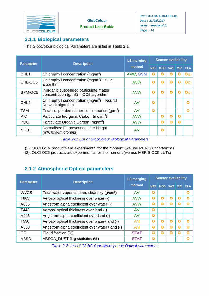
2.1.1 Biological parameters

The GlobColour biological Parameters are listed in Table 2-1.

Parameter Description L3 merging

method

Sensor availability

MER MOD SWF VIR OLA

CHL1 Chlorophyll concentration (mg/m3) AVW, GSM (1)

CHL-OC5 Chlorophyll concentration (mg/m3) – OC5 algorithm

AVW (2)

SPM-OC5 Inorganic suspended particulate matter concentration (g/m3) – OC5 algorithm

AVW (2)

CHL2 Chlorophyll concentration (mg/m3) – Neural Network algorithm

AV

TSM Total suspended matter concentration (g/m3) AV

PIC Particulate Inorganic Carbon (mol/m3) AVW

POC Particulate Organic Carbon (mg/m3) AVW

NFLH Normalised Fluorescence Line Height (mW/cm²/microm/sr)

AV

Table 2-1: List of GlobColour Biological Parameters (1): OLCI GSM products are experimental for the moment (we use MERIS uncertainties) (2): OLCI OC5 products are experimental for the moment (we use MERIS OC5 LUTs)

2.1.2 Atmospheric Optical parameters


method

Sensor availability

MER MOD SWF VIR OLA

WVCS Total water vapor column, clear sky (g/cm²) AV

T865 Aerosol optical thickness over water (-) AVW

A865 Angstrom alpha coefficient over water (-) AVW

T443 Aerosol optical thickness over land (-) AV

A443 Angstrom alpha coefficient over land (-) AV

T550 Aerosol optical thickness over water+land (-) AN

A550 Angstrom alpha coefficient over water+land (-) AN

CF Cloud fraction (%) STAT

ABSD ABSOA_DUST flag statistics (%) STAT

Table 2-2: List of GlobColour Atmospheric Optical parameters

GlobColour

Product User Guide


Date : 31/08/2017

Issue : version 4.1

Page : 15

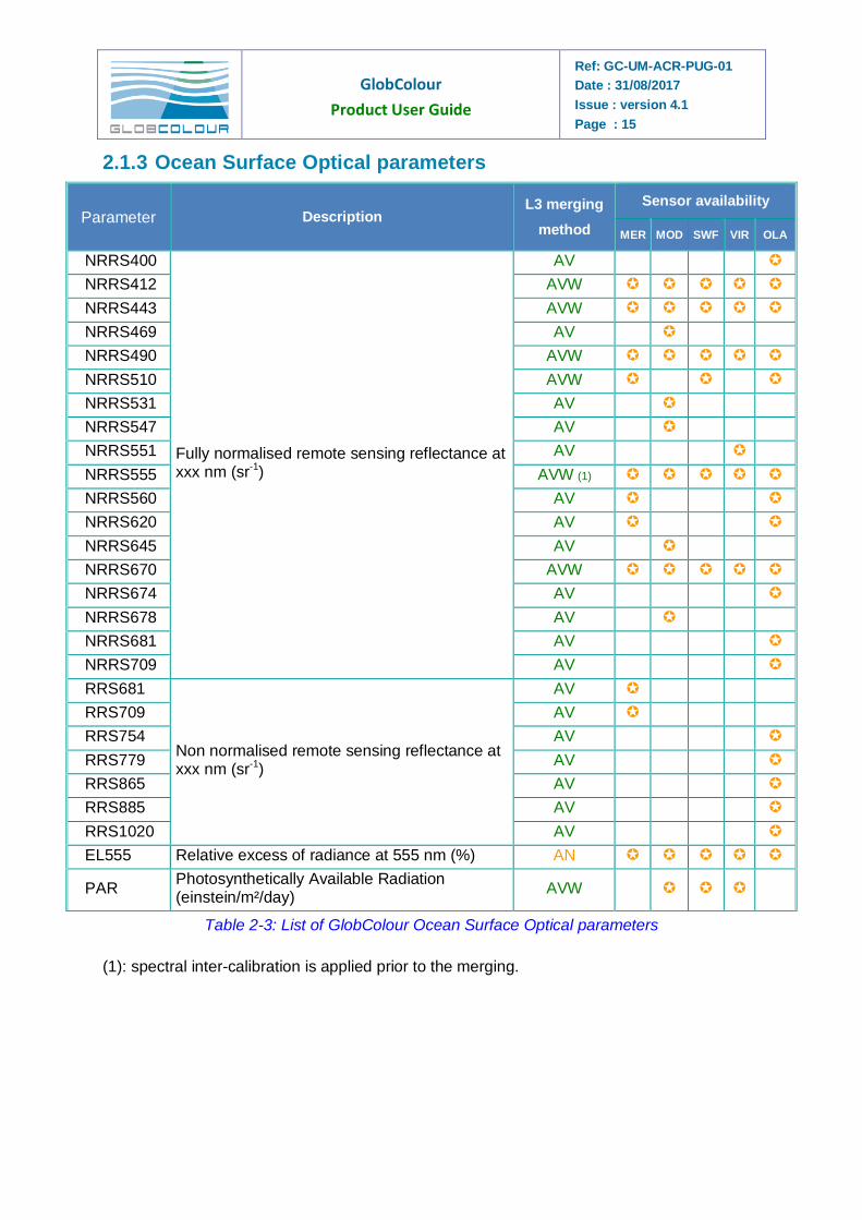
2.1.3 Ocean Surface Optical parameters


method

Sensor availability

MER MOD SWF VIR OLA

NRRS400

Fully normalised remote sensing reflectance at xxx nm (sr-1)

AV

NRRS412 AVW

NRRS443 AVW

NRRS469 AV

NRRS490 AVW

NRRS510 AVW

NRRS531 AV

NRRS547 AV

NRRS551 AV

NRRS555 AVW (1)

NRRS560 AV

NRRS620 AV

NRRS645 AV

NRRS670 AVW

NRRS674 AV

NRRS678 AV

NRRS681 AV

NRRS709 AV

RRS681

Non normalised remote sensing reflectance at xxx nm (sr-1)

AV

RRS709 AV

RRS754 AV

RRS779 AV

RRS865 AV

RRS885 AV

RRS1020 AV

EL555 Relative excess of radiance at 555 nm (%) AN

PAR Photosynthetically Available Radiation (einstein/m²/day)

AVW

Table 2-3: List of GlobColour Ocean Surface Optical parameters

(1): spectral inter-calibration is applied prior to the merging.

GlobColour

Product User Guide


Date : 31/08/2017

Issue : version 4.1

Page : 16

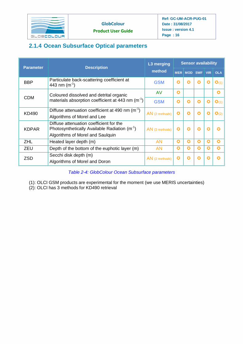
2.1.4 Ocean Subsurface Optical parameters


method

Sensor availability

MER MOD SWF VIR OLA

BBP Particulate back-scattering coefficient at 443 nm (m-1)

GSM (1)

CDM Coloured dissolved and detrital organic materials absorption coefficient at 443 nm (m-1)

AV

GSM (1)

KD490 Diffuse attenuation coefficient at 490 nm (m-1)

Algorithms of Morel and Lee AN (2 methods) (2)

KDPAR

Diffuse attenuation coefficient for the Photosynthetically Available Radiation (m-1)

Algorithms of Morel and Saulquin

AN (2 methods)

ZHL Heated layer depth (m) AN

ZEU Depth of the bottom of the euphotic layer (m) AN

ZSD Secchi disk depth (m)

Algorithms of Morel and Doron AN (2 methods)

Table 2-4: GlobColour Ocean Subsurface parameters (1): OLCI GSM products are experimental for the moment (we use MERIS uncertainties) (2): OLCI has 3 methods for KD490 retrieval

GlobColour

Product User Guide


Date : 31/08/2017

Issue : version 4.1

Page : 17

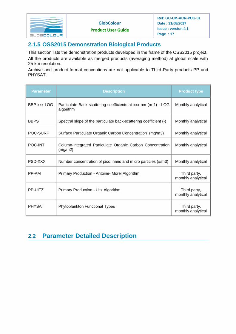
2.1.5 OSS2015 Demonstration Biological Products

This section lists the demonstration products developed in the frame of the OSS2015 project.

All the products are available as merged products (averaging method) at global scale with 25 km resolution.

Archive and product format conventions are not applicable to Third-Party products PP and PHYSAT.

Parameter Description Product type

BBP-xxx-LOG Particulate Back-scattering coefficients at xxx nm (m-1) - LOG algorithm

Monthly analytical

BBPS Spectral slope of the particulate back-scattering coefficient (-) Monthly analytical

POC-SURF Surface Particulate Organic Carbon Concentration (mg/m3) Monthly analytical

POC-INT Column-integrated Particulate Organic Carbon Concentration (mg/m2)

Monthly analytical

PSD-XXX Number concentration of pico, nano and micro particles (#/m3) Monthly analytical

PP-AM Primary Production - Antoine- Morel Algorithm Third party, monthly analytical

PP-UITZ Primary Production - Uitz Algorithm Third party, monthly analytical

PHYSAT Phytoplankton Functional Types Third party, monthly analytical

2.2 Parameter Detailed Description

GlobColour

Product User Guide


Date : 31/08/2017

Issue : version 4.1

Page : 18

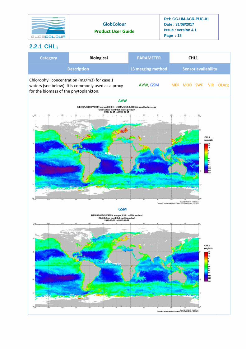
2.2.1 CHL1

Category Biological PARAMETER CHL1

Description L3 merging method Sensor availability

Chlorophyll concentration (mg/m3) for case 1 waters (see below). It is commonly used as a proxy for the biomass of the phytoplankton.

AVW, GSM MER MOD SWF VIR OLA(1)

AVW

GSM

GlobColour

Product User Guide


Date : 31/08/2017

Issue : version 4.1

Page : 19

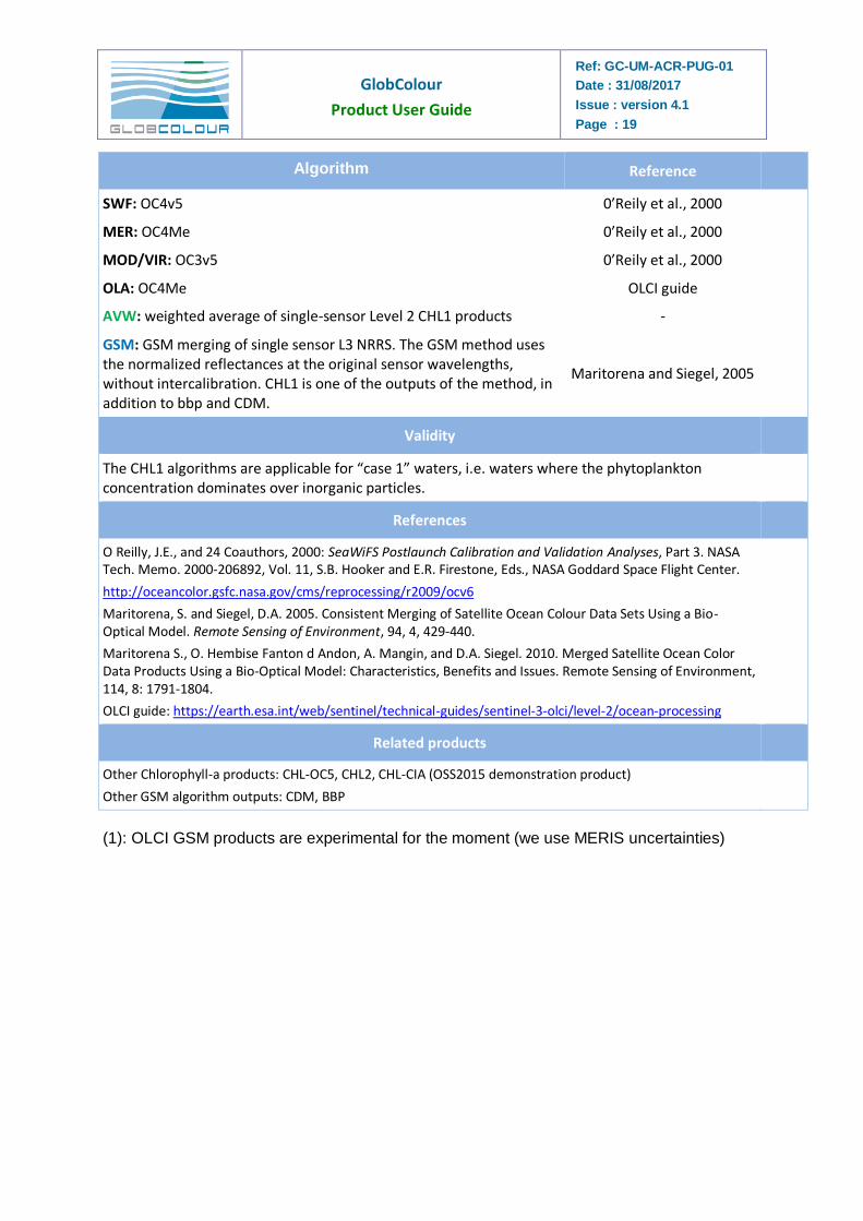
Algorithm Reference

SWF: OC4v5 0’Reily et al., 2000

MER: OC4Me 0’Reily et al., 2000

MOD/VIR: OC3v5 0’Reily et al., 2000

OLA: OC4Me OLCI guide

AVW: weighted average of single-sensor Level 2 CHL1 products -

GSM: GSM merging of single sensor L3 NRRS. The GSM method uses the normalized reflectances at the original sensor wavelengths, without intercalibration. CHL1 is one of the outputs of the method, in addition to bbp and CDM.

Maritorena and Siegel, 2005

Validity

The CHL1 algorithms are applicable for “case 1” waters, i.e. waters where the phytoplankton concentration dominates over inorganic particles.

References

O Reilly, J.E., and 24 Coauthors, 2000: SeaWiFS Postlaunch Calibration and Validation Analyses, Part 3. NASA Tech. Memo. 2000-206892, Vol. 11, S.B. Hooker and E.R. Firestone, Eds., NASA Goddard Space Flight Center.

http://oceancolor.gsfc.nasa.gov/cms/reprocessing/r2009/ocv6

Maritorena, S. and Siegel, D.A. 2005. Consistent Merging of Satellite Ocean Colour Data Sets Using a Bio-Optical Model. Remote Sensing of Environment, 94, 4, 429-440.

Maritorena S., O. Hembise Fanton d Andon, A. Mangin, and D.A. Siegel. 2010. Merged Satellite Ocean Color Data Products Using a Bio-Optical Model: Characteristics, Benefits and Issues. Remote Sensing of Environment, 114, 8: 1791-1804.

OLCI guide: https://earth.esa.int/web/sentinel/technical-guides/sentinel-3-olci/level-2/ocean-processing

Related products

Other Chlorophyll-a products: CHL-OC5, CHL2, CHL-CIA (OSS2015 demonstration product)

Other GSM algorithm outputs: CDM, BBP

(1): OLCI GSM products are experimental for the moment (we use MERIS uncertainties)

http://oceancolor.gsfc.nasa.gov/cms/reprocessing/r2009/ocv6

https://earth.esa.int/web/sentinel/technical-guides/sentinel-3-olci/level-2/ocean-processing

GlobColour

Product User Guide


Date : 31/08/2017

Issue : version 4.1

Page : 20

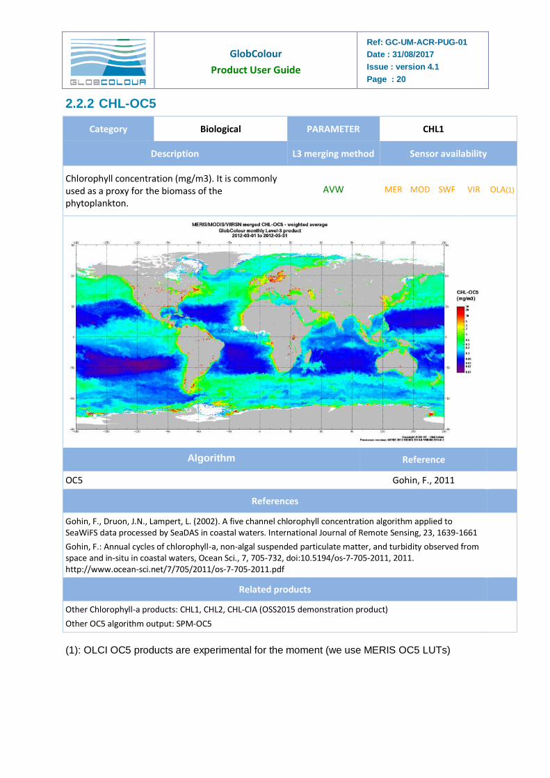
2.2.2 CHL-OC5



Chlorophyll concentration (mg/m3). It is commonly used as a proxy for the biomass of the phytoplankton.

AVW MER MOD SWF VIR OLA(1)

Algorithm Reference

OC5 Gohin, F., 2011

References

Gohin, F., Druon, J.N., Lampert, L. (2002). A five channel chlorophyll concentration algorithm applied to SeaWiFS data processed by SeaDAS in coastal waters. International Journal of Remote Sensing, 23, 1639-1661

Gohin, F.: Annual cycles of chlorophyll-a, non-algal suspended particulate matter, and turbidity observed from space and in-situ in coastal waters, Ocean Sci., 7, 705-732, doi:10.5194/os-7-705-2011, 2011. http://www.ocean-sci.net/7/705/2011/os-7-705-2011.pdf

Related products

Other Chlorophyll-a products: CHL1, CHL2, CHL-CIA (OSS2015 demonstration product)

Other OC5 algorithm output: SPM-OC5

(1): OLCI OC5 products are experimental for the moment (we use MERIS OC5 LUTs)

GlobColour

Product User Guide


Date : 31/08/2017

Issue : version 4.1

Page : 21

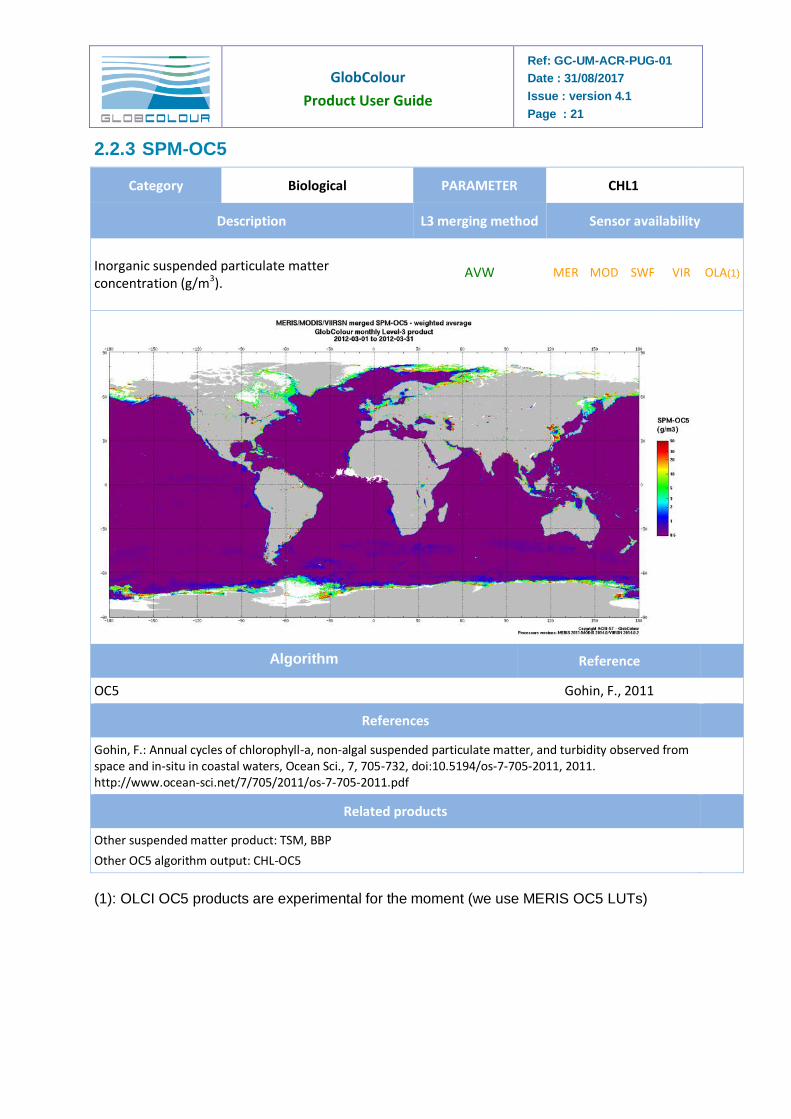
2.2.3 SPM-OC5



Inorganic suspended particulate matter concentration (g/m3).

AVW MER MOD SWF VIR OLA(1)

Algorithm Reference

OC5 Gohin, F., 2011

References


Related products

Other suspended matter product: TSM, BBP

Other OC5 algorithm output: CHL-OC5

(1): OLCI OC5 products are experimental for the moment (we use MERIS OC5 LUTs)

GlobColour

Product User Guide


Date : 31/08/2017

Issue : version 4.1

Page : 22

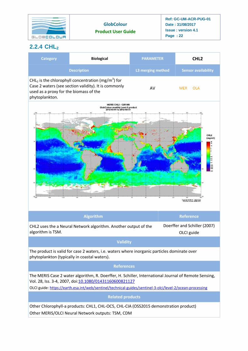
2.2.4 CHL2



CHL2 is the chlorophyll concentration (mg/m3) for Case 2 waters (see section validity). It is commonly used as a proxy for the biomass of the phytoplankton.

AV MER OLA

Algorithm Reference

CHL2 uses the a Neural Network algorithm. Another output of the algorithm is TSM.

Doerffer and Schiller (2007)

OLCI guide

Validity

The product is valid for case 2 waters, i.e. waters where inorganic particles dominate over phytoplankton (typically in coastal waters).

References

The MERIS Case 2 water algorithm, R. Doerffer, H. Schiller, International Journal of Remote Sensing, Vol. 28, Iss. 3-4, 2007, doi:10.1080/01431160600821127


Related products

Other Chlorophyll-a products: CHL1, CHL-OC5, CHL-CIA (OSS2015 demonstration product)

Other MERIS/OLCI Neural Network outputs: TSM, CDM

http://dx.doi.org/10.1080/01431160600821127


GlobColour

Product User Guide


Date : 31/08/2017

Issue : version 4.1

Page : 23

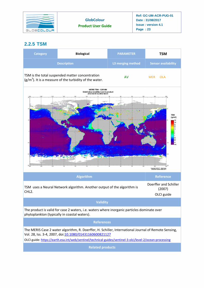
2.2.5 TSM

Category Biological PARAMETER TSM


TSM is the total suspended matter concentration (g/m3). It is a measure of the turbidity of the water.

AV MER OLA

Algorithm Reference

TSM uses a Neural Network algorithm. Another output of the algorithm is CHL2.


OLCI guide

Validity

The product is valid for case 2 waters, i.e. waters where inorganic particles dominate over phytoplankton (typically in coastal waters).

References



Related products

http://dx.doi.org/10.1080/01431160600821127


GlobColour

Product User Guide


Date : 31/08/2017

Issue : version 4.1

Page : 24

The MERIS/OLCI TSM product is computed from the back-scattering coefficient at 444 nm using the following assumptions: BP = BBP/0.015, TSM = 1.73*BP. Therefore the BBP variable issued from the GSM algorithm is closely related to TSM. SPM-OC5 provides the inorganic suspended particulate matter, a product closely linked to TSM, according to the OC5 algorithm.

Other MERIS/OLCI Neural Network outputs: CHL2, CDM

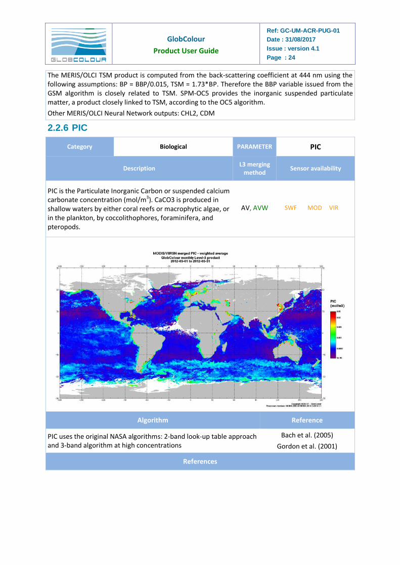
2.2.6 PIC

Category Biological PARAMETER PIC

Description L3 merging

method Sensor availability

PIC is the Particulate Inorganic Carbon or suspended calcium carbonate concentration (mol/m3). CaCO3 is produced in shallow waters by either coral reefs or macrophytic algae, or in the plankton, by coccolithophores, foraminifera, and pteropods.

AV, AVW SWF MOD VIR

Algorithm Reference

PIC uses the original NASA algorithms: 2-band look-up table approach and 3-band algorithm at high concentrations

Bach et al. (2005)

Gordon et al. (2001)

References

GlobColour

Product User Guide


Date : 31/08/2017

Issue : version 4.1

Page : 25

Balch, W. M., H. R. Gordon, B. C. Bowler, D. T. Drapeau, and E. S. Booth. (2005) Calcium carbonate measurements in the surface global ocean based on Moderate-Resolution Imaging Spectroradiometer data, JGR, Vol. 110, C07001 http://dx.doi.org/10.1029/2004JC002560

Gordon, Howard R., G. Chris Boynton, William M. Balch, Stephen B. Groom, Derek S. Harbour, and Tim J. Smyth. (2001) Retrieval of Coccolithophore Calcite Concentration from SeaWiFS Imagery. GRL, Vol. 28, No. 8, pp. 1587-1590 http://dx.doi.org/10.1029/2000GL012025

Related products

POC provides the Particulate Organic Concentration

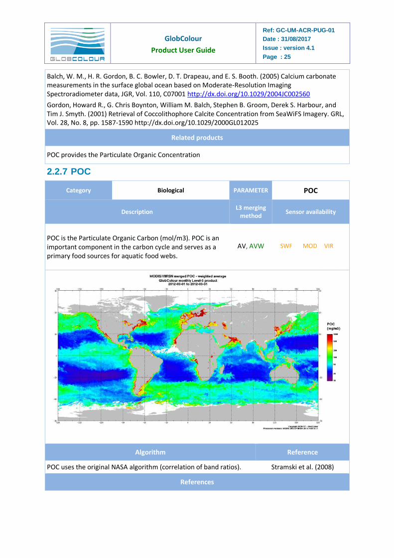
2.2.7 POC

Category Biological PARAMETER POC



POC is the Particulate Organic Carbon (mol/m3). POC is an important component in the carbon cycle and serves as a primary food sources for aquatic food webs.

AV, AVW SWF MOD VIR

Algorithm Reference

POC uses the original NASA algorithm (correlation of band ratios). Stramski et al. (2008)

References

http://dx.doi.org/10.1029/2004JC002560

GlobColour

Product User Guide


Date : 31/08/2017

Issue : version 4.1

Page : 26

Stramski. D., R.A. Reynolds, M. Babin, S. Kaczmarek, M.R. Lewis, R. Rottgers, A. Sciandra, M. Stramska, M.S. Twardowski, B.A. Franz, and H. Claustre (2008). Relationships between the surface concentration of particulate organic carbon and optical properties in the eastern South Pacific and eastern Atlantic Oceans, Biogeosci., 5, 171-201.

Related products

PIC provides the Particulate Inorganic Concentration

The OSS2015 archive includes a similar POC product and a column-integrated POC product.

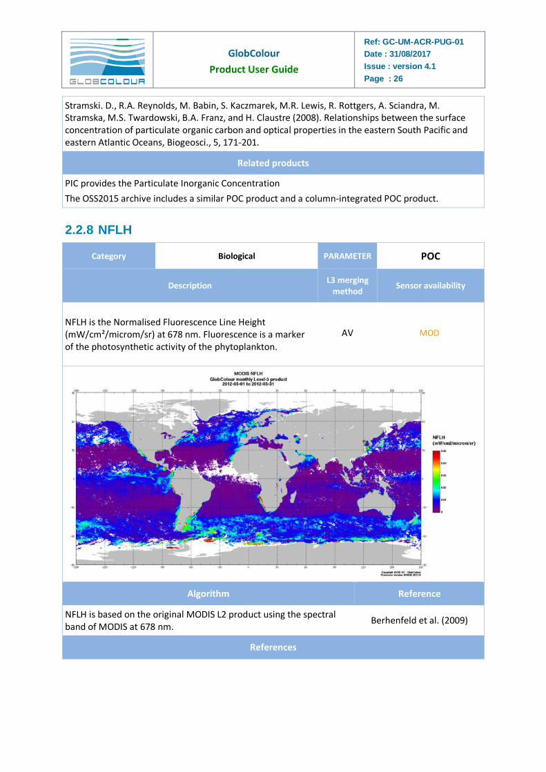
2.2.8 NFLH

Category Biological PARAMETER POC



NFLH is the Normalised Fluorescence Line Height (mW/cm²/microm/sr) at 678 nm. Fluorescence is a marker of the photosynthetic activity of the phytoplankton.

AV MOD

Algorithm Reference

NFLH is based on the original MODIS L2 product using the spectral band of MODIS at 678 nm.

Berhenfeld et al. (2009)

References

GlobColour

Product User Guide


Date : 31/08/2017

Issue : version 4.1

Page : 27

Behrenfeld, M.J., T.K. Westberry, E.S. Boss, R.T. O Malley, D.A. Siegel, J.D. Wiggert, B.A. Franz, C.R. McClain, G.C. Feldman, S.C. Doney, J.K. Moore, G. Dall Olmo, A. J. Milligan, I. Lima, and N. Mahowald (2009). Satellite-detected fluorescence reveals global physiology of ocean phytoplankton, Biogeosci., 6, 779-794.

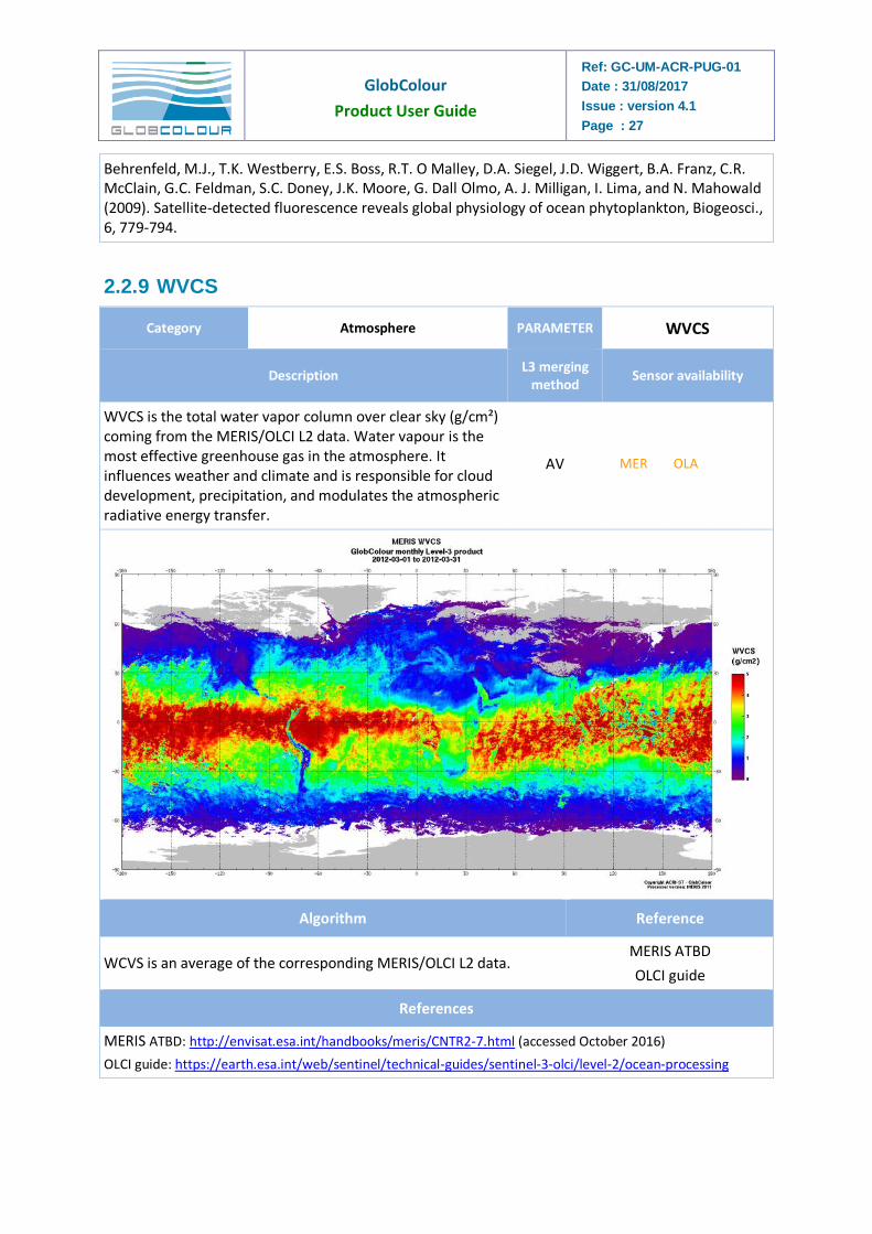
2.2.9 WVCS

Category Atmosphere PARAMETER WVCS



WVCS is the total water vapor column over clear sky (g/cm²) coming from the MERIS/OLCI L2 data. Water vapour is the most effective greenhouse gas in the atmosphere. It influences weather and climate and is responsible for cloud development, precipitation, and modulates the atmospheric radiative energy transfer.

AV MER OLA

Algorithm Reference

WCVS is an average of the corresponding MERIS/OLCI L2 data. MERIS ATBD

OLCI guide

References

MERIS ATBD: http://envisat.esa.int/handbooks/meris/CNTR2-7.html (accessed October 2016)


http://envisat.esa.int/handbooks/meris/CNTR2-7.html


GlobColour

Product User Guide


Date : 31/08/2017

Issue : version 4.1

Page : 28

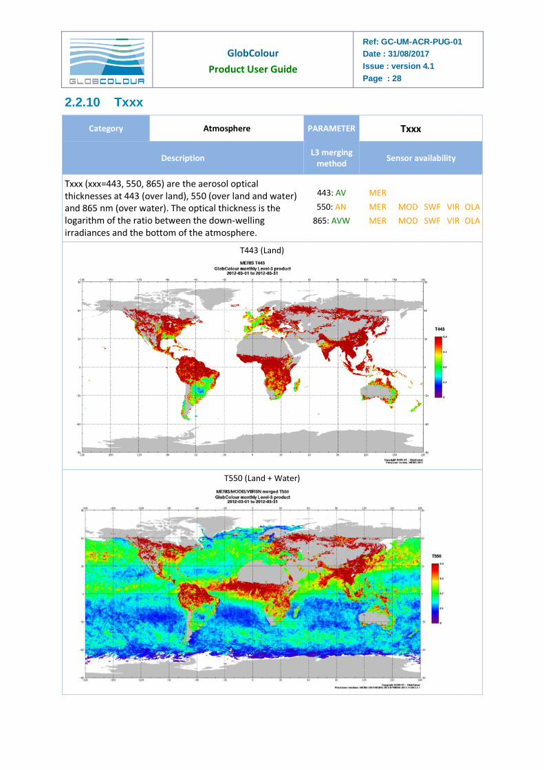
2.2.10 Txxx

Category Atmosphere PARAMETER Txxx



Txxx (xxx=443, 550, 865) are the aerosol optical thicknesses at 443 (over land), 550 (over land and water) and 865 nm (over water). The optical thickness is the logarithm of the ratio between the down-welling irradiances and the bottom of the atmosphere.

443: AV

550: AN

865: AVW

MER

MER

MER

MOD

MOD

SWF

SWF

VIR

VIR

OLA

OLA

T443 (Land)

T550 (Land + Water)

GlobColour

Product User Guide


Date : 31/08/2017

Issue : version 4.1

Page : 29

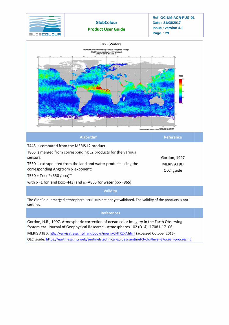
T865 (Water)

Algorithm Reference

T443 is computed from the MERIS L2 product.

T865 is merged from corresponding L2 products for the various sensors.

T550 is extrapolated from the land and water products using the

corresponding Angström exponent:

T550 = Txxx * (550 / xxx)-

with =1 for land (xxx=443) and =A865 for water (xxx=865)

Gordon, 1997

MERIS ATBD

OLCI guide

Validity

The GlobColour merged atmosphere products are not yet validated. The validity of the products is not certified.

References

Gordon, H.R., 1997. Atmospheric correction of ocean color imagery in the Earth Observing System era. Journal of Geophysical Research - Atmospheres 102 (D14), 17081-17106





GlobColour

Product User Guide


Date : 31/08/2017

Issue : version 4.1

Page : 30

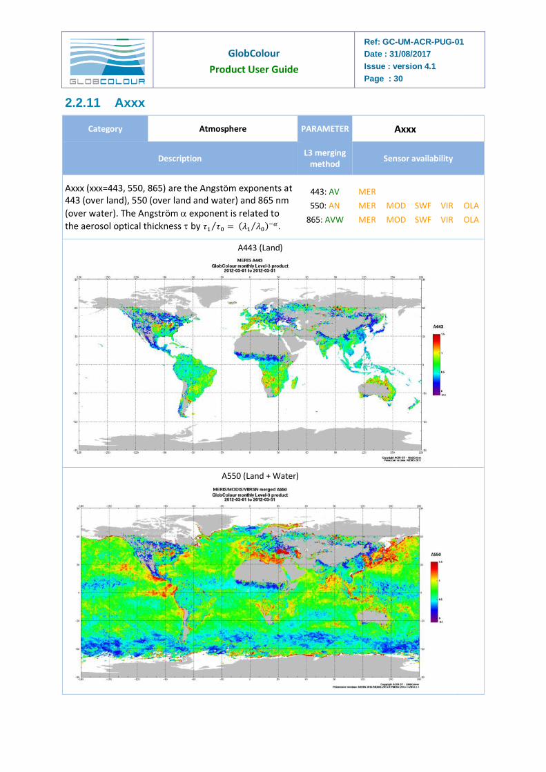
2.2.11 Axxx

Category Atmosphere PARAMETER Axxx



Axxx (xxx=443, 550, 865) are the Angstöm exponents at 443 (over land), 550 (over land and water) and 865 nm

(over water). The Angström exponent is related to

the aerosol optical thickness by 𝜏1 𝜏0 = (𝜆1 𝜆0⁄ )−𝛼⁄ .

443: AV

550: AN

865: AVW

MER

MER

MER

MOD

MOD

SWF

SWF

VIR

VIR

OLA

OLA

A443 (Land)

A550 (Land + Water)

GlobColour

Product User Guide


Date : 31/08/2017

Issue : version 4.1

Page : 31

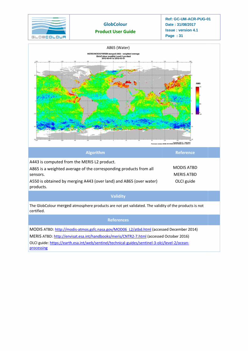
A865 (Water)

Algorithm Reference

A443 is computed from the MERIS L2 product.

A865 is a weighted average of the corresponding products from all sensors.

A550 is obtained by merging A443 (over land) and A865 (over water) products.

MODIS ATBD

MERIS ATBD

OLCI guide

Validity

The GlobColour merged atmosphere products are not yet validated. The validity of the products is not certified.

References

MODIS ATBD: http://modis-atmos.gsfc.nasa.gov/MOD06_L2/atbd.html (accessed December 2014)



http://modis-atmos.gsfc.nasa.gov/MOD06_L2/atbd.html




GlobColour

Product User Guide


Date : 31/08/2017

Issue : version 4.1

Page : 32

2.2.12 CF

Category Atmosphere PARAMETER CF



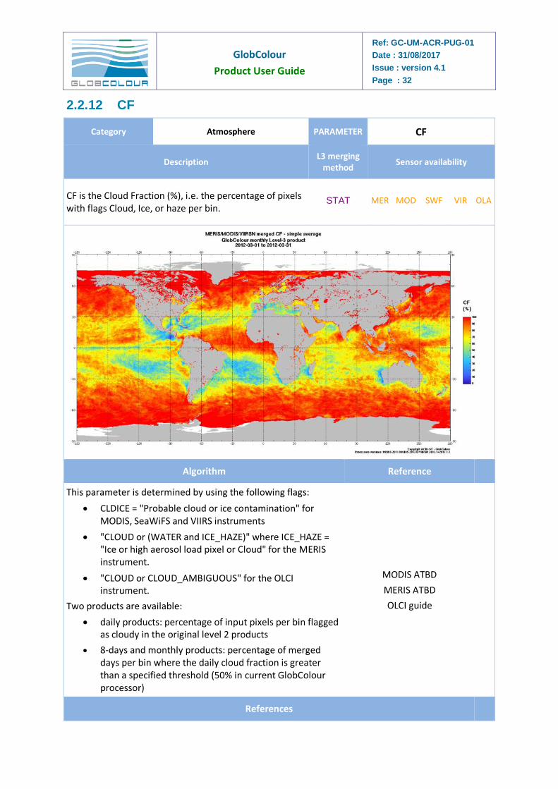
CF is the Cloud Fraction (%), i.e. the percentage of pixels with flags Cloud, Ice, or haze per bin.

STAT MER MOD SWF VIR OLA

Algorithm Reference

This parameter is determined by using the following flags:

CLDICE = "Probable cloud or ice contamination" for MODIS, SeaWiFS and VIIRS instruments

"CLOUD or (WATER and ICE_HAZE)" where ICE_HAZE = "Ice or high aerosol load pixel or Cloud" for the MERIS instrument.

"CLOUD or CLOUD_AMBIGUOUS" for the OLCI instrument.

Two products are available:

daily products: percentage of input pixels per bin flagged as cloudy in the original level 2 products

8-days and monthly products: percentage of merged days per bin where the daily cloud fraction is greater than a specified threshold (50% in current GlobColour processor)

MODIS ATBD

MERIS ATBD

OLCI guide

References

GlobColour

Product User Guide


Date : 31/08/2017

Issue : version 4.1

Page : 33

MODIS ATBD: http://modis-atmos.gsfc.nasa.gov/MOD06_L2/atbd.html (accessed December 2014)



2.2.13 ABSD

Category Atmosphere PARAMETER ABSD



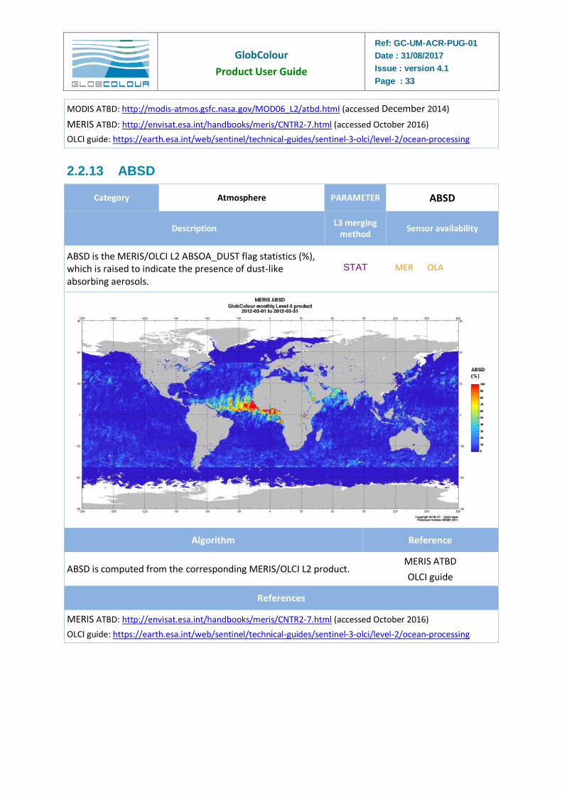
ABSD is the MERIS/OLCI L2 ABSOA_DUST flag statistics (%), which is raised to indicate the presence of dust-like absorbing aerosols.

STAT MER OLA

Algorithm Reference

ABSD is computed from the corresponding MERIS/OLCI L2 product. MERIS ATBD

OLCI guide

References



http://modis-atmos.gsfc.nasa.gov/MOD06_L2/atbd.html





GlobColour

Product User Guide


Date : 31/08/2017

Issue : version 4.1

Page : 34

2.2.14 (N)RRSxxx

Category Ocean Surface Optical PARAMETER (N)RRSxxx



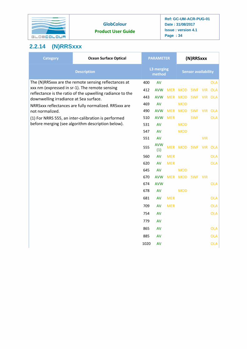
The (N)RRSxxx are the remote sensing reflectances at xxx nm (expressed in sr-1). The remote sensing reflectance is the ratio of the upwelling radiance to the downwelling irradiance at Sea surface.

NRRSxxx reflectances are fully normalized. RRSxxx are not normalized.

(1) For NRRS 555, an inter-calibration is performed before merging (see algorithm description below).

400 AV OLA

412 AVW MER MOD SWF VIR OLA


469 AV

MOD


510 AVW MER

SWF

OLA

531 AV

MOD

547 AV

MOD

551 AV

VIR

555 AVW

(1) MER MOD SWF VIR OLA

560 AV MER

OLA

620 AV MER

OLA

645 AV

MOD

670 AVW MER MOD SWF VIR

674 AVW OLA

678 AV

MOD

681 AV MER

OLA

709 AV MER

OLA

754 AV OLA

779 AV

865 AV OLA

885 AV OLA

1020 AV OLA

GlobColour

Product User Guide


Date : 31/08/2017

Issue : version 4.1

Page : 35

Algorithm

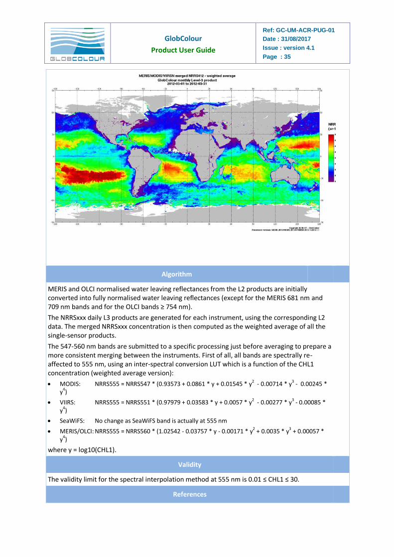
MERIS and OLCI normalised water leaving reflectances from the L2 products are initially converted into fully normalised water leaving reflectances (except for the MERIS 681 nm and 709 nm bands and for the OLCI bands ≥ 754 nm).

The NRRSxxx daily L3 products are generated for each instrument, using the corresponding L2 data. The merged NRRSxxx concentration is then computed as the weighted average of all the single-sensor products.

The 547-560 nm bands are submitted to a specific processing just before averaging to prepare a more consistent merging between the instruments. First of all, all bands are spectrally re-affected to 555 nm, using an inter-spectral conversion LUT which is a function of the CHL1 concentration (weighted average version):

MODIS: NRRS555 = NRRS547 * (0.93573 + 0.0861 * y + 0.01545 * y2 - 0.00714 * y3 - 0.00245 * y4)

VIIRS: NRRS555 = NRRS551 * (0.97979 + 0.03583 * y + 0.0057 * y2 - 0.00277 * y3 - 0.00085 * y4)

SeaWiFS: No change as SeaWiFS band is actually at 555 nm

MERIS/OLCI: NRRS555 = NRRS560 * (1.02542 - 0.03757 * y - 0.00171 * y2 + 0.0035 * y3 + 0.00057 * y

4)

where y = log10(CHL1).

Validity

The validity limit for the spectral interpolation method at 555 nm is 0.01 ≤ CHL1 ≤ 30.

References

GlobColour

Product User Guide


Date : 31/08/2017

Issue : version 4.1

Page : 36

N/A

GlobColour

Product User Guide


Date : 31/08/2017

Issue : version 4.1

Page : 37

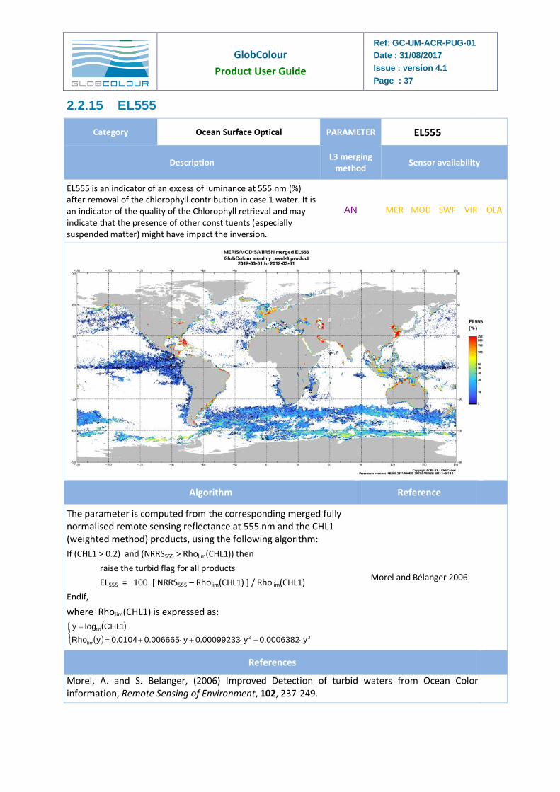
2.2.15 EL555

Category Ocean Surface Optical PARAMETER EL555



EL555 is an indicator of an excess of luminance at 555 nm (%) after removal of the chlorophyll contribution in case 1 water. It is an indicator of the quality of the Chlorophyll retrieval and may indicate that the presence of other constituents (especially suspended matter) might have impact the inversion.

AN MER MOD SWF VIR OLA

Algorithm Reference

The parameter is computed from the corresponding merged fully normalised remote sensing reflectance at 555 nm and the CHL1 (weighted method) products, using the following algorithm:

If (CHL1 > 0.2) and (NRRS555 > Rholim(CHL1)) then

raise the turbid flag for all products

EL555 = 100. [ NRRS555 – Rholim(CHL1) ] / Rholim(CHL1)

Endif,

where Rholim(CHL1) is expressed as:

32

lim

10

y0006382.0y00099233.0y006665.00104.0yRho

1CHLlogy

Morel and Bélanger 2006

References

Morel, A. and S. Belanger, (2006) Improved Detection of turbid waters from Ocean Color information, Remote Sensing of Environment, 102, 237-249.

GlobColour

Product User Guide


Date : 31/08/2017

Issue : version 4.1

Page : 38

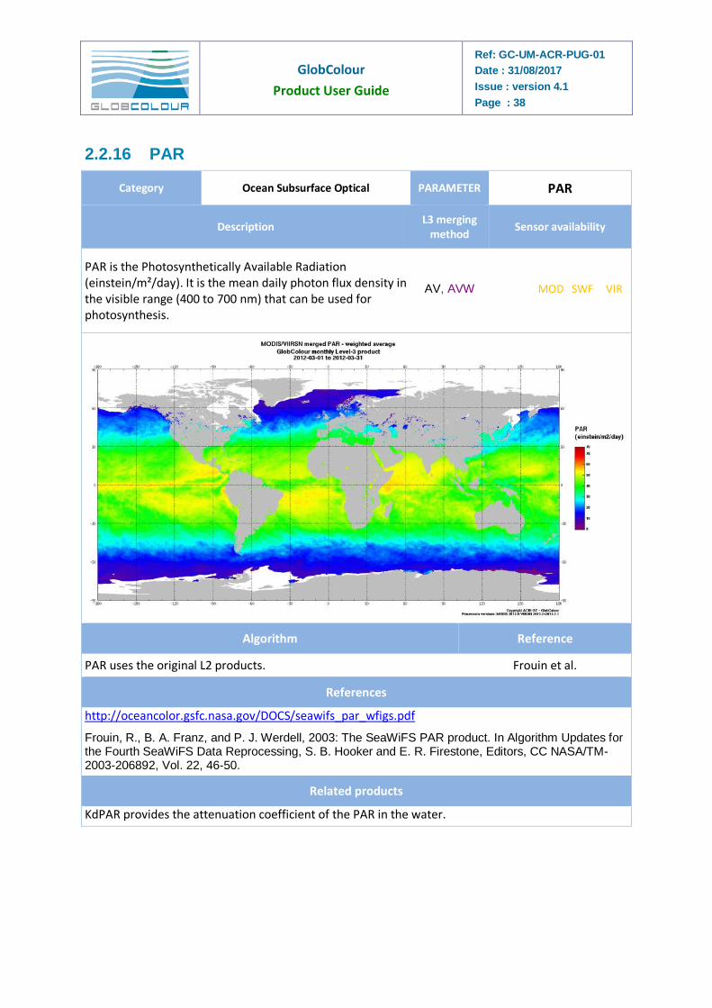
2.2.16 PAR

Category Ocean Subsurface Optical PARAMETER PAR



PAR is the Photosynthetically Available Radiation (einstein/m²/day). It is the mean daily photon flux density in the visible range (400 to 700 nm) that can be used for photosynthesis.

AV, AVW MOD SWF VIR

Algorithm Reference

PAR uses the original L2 products. Frouin et al.

References

http://oceancolor.gsfc.nasa.gov/DOCS/seawifs_par_wfigs.pdf

Frouin, R., B. A. Franz, and P. J. Werdell, 2003: The SeaWiFS PAR product. In Algorithm Updates for the Fourth SeaWiFS Data Reprocessing, S. B. Hooker and E. R. Firestone, Editors, CC NASA/TM-2003-206892, Vol. 22, 46-50.

Related products

KdPAR provides the attenuation coefficient of the PAR in the water.

http://oceancolor.gsfc.nasa.gov/DOCS/seawifs_par_wfigs.pdf

GlobColour

Product User Guide


Date : 31/08/2017

Issue : version 4.1

Page : 39

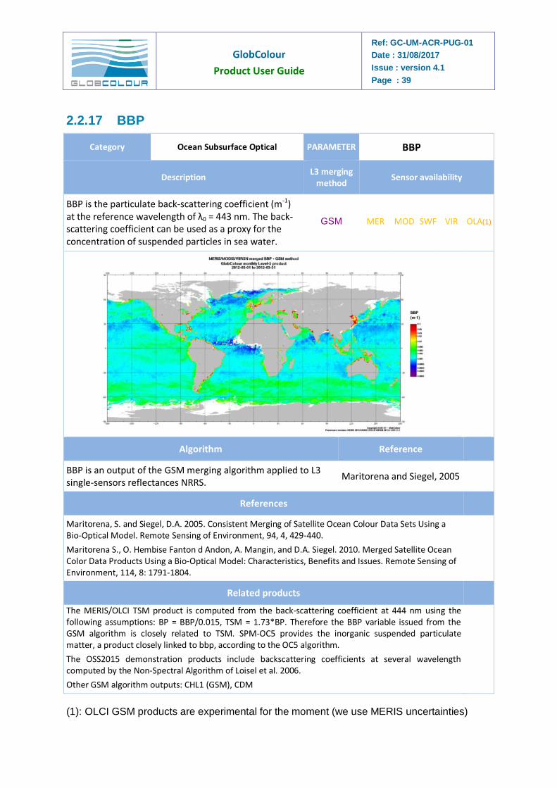
2.2.17 BBP

Category Ocean Subsurface Optical PARAMETER BBP



BBP is the particulate back-scattering coefficient (m-1) at the reference wavelength of λ0 = 443 nm. The back-scattering coefficient can be used as a proxy for the concentration of suspended particles in sea water.

GSM MER MOD SWF VIR OLA(1)

Algorithm Reference

BBP is an output of the GSM merging algorithm applied to L3 single-sensors reflectances NRRS.

Maritorena and Siegel, 2005

References



Related products

The MERIS/OLCI TSM product is computed from the back-scattering coefficient at 444 nm using the following assumptions: BP = BBP/0.015, TSM = 1.73*BP. Therefore the BBP variable issued from the GSM algorithm is closely related to TSM. SPM-OC5 provides the inorganic suspended particulate matter, a product closely linked to bbp, according to the OC5 algorithm.

The OSS2015 demonstration products include backscattering coefficients at several wavelength computed by the Non-Spectral Algorithm of Loisel et al. 2006.

Other GSM algorithm outputs: CHL1 (GSM), CDM


GlobColour

Product User Guide


Date : 31/08/2017

Issue : version 4.1

Page : 40

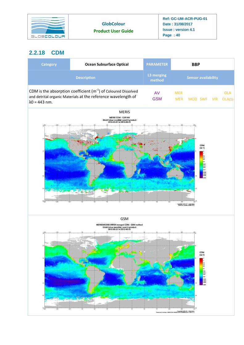
2.2.18 CDM

Category Ocean Subsurface Optical PARAMETER BBP



CDM is the absorption coefficient (m-1) of Coloured Dissolved

and detrital organic Materials at the reference wavelength of λ0 = 443 nm.

AV

GSM

MER

MER

MOD

SWF

VIR

OLA

OLA(1)

MERIS

GSM

GlobColour

Product User Guide


Date : 31/08/2017

Issue : version 4.1

Page : 41

Algorithm Reference

MER: MERIS Neural Network algorithm

OLA: OLCI Neural Network algorithm


OLCI guide

GSM: GSM merging of single sensor L3 NRRS. The GSM method uses the normalized reflectances at the original sensor wavelengths, without intercalibration. CDM is one of the outputs of the method, in addition to BBP and CHL1.

Maritorena et al. 2010

References





Related products

Other MERIS/OLCI Neural Network outputs: CHL2, TSM

Other GSM algorithm outputs: CHL1 (GSM), BBP




GlobColour

Product User Guide


Date : 31/08/2017

Issue : version 4.1

Page : 42

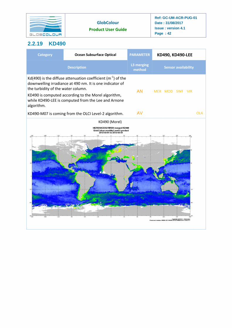
2.2.19 KD490

Category Ocean Subsurface Optical PARAMETER KD490, KD490-LEE



Kd(490) is the diffuse attenuation coefficient (m-1) of the downwelling irradiance at 490 nm. It is one indicator of the turbidity of the water column.

KD490 is computed according to the Morel algorithm, while KD490-LEE is computed from the Lee and Arnone algorithm.

AN MER MOD SWF VIR

KD490-M07 is coming from the OLCI Level-2 algorithm. AV OLA

KD490 (Morel)

GlobColour

Product User Guide


Date : 31/08/2017

Issue : version 4.1

Page : 43

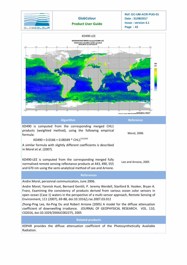
KD490-LEE

Algorithm Reference

KD490 is computed from the corresponding merged CHL1 products (weighted method), using the following empirical formula:

KD490 = 0.0166 + 0.08349 * CHL10.63303

A similar formula with slightly different coefficients is described in Morel et al. (2007).

KD490-LEE is computed from the corresponding merged fully normalised remote sensing reflectance products at 443, 490, 555 and 670 nm using the semi-analytical method of Lee and Arnone.

Morel, 2006

Lee and Arnone, 2005

References

Andre Morel, personnal communication, June 2006.

Andre Morel, Yannick Huot, Bernard Gentili, P. Jeremy Werdell, Stanford B. Hooker, Bryan A. Franz, Examining the consistency of products derived from various ocean color sensors in open ocean (Case 1) waters in the perspective of a multi-sensor approach, Remote Sensing of Environment, 111 (2007), 69-88, doi:10.1016/j.rse.2007.03.012

Zhong-Ping Lee, Ke-Ping Du and Robert Arnone (2005) A model for the diffuse attenuation coefficient of downwelling irradiance. JOURNAL OF GEOPHYSICAL RESEARCH. VOL. 110, C02016, doi:10.1029/2004JC002275, 2005

Related products

KDPAR provides the diffuse attenuation coefficient of the Photosynthetically Available Radiation.

GlobColour

Product User Guide


Date : 31/08/2017

Issue : version 4.1

Page : 44

GlobColour

Product User Guide


Date : 31/08/2017

Issue : version 4.1

Page : 45

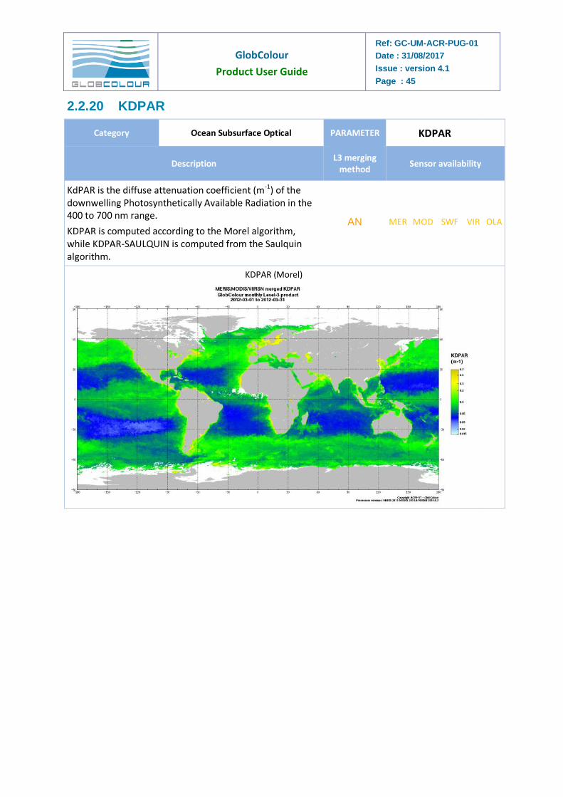
2.2.20 KDPAR

Category Ocean Subsurface Optical PARAMETER KDPAR



KdPAR is the diffuse attenuation coefficient (m-1) of the downwelling Photosynthetically Available Radiation in the 400 to 700 nm range.

KDPAR is computed according to the Morel algorithm, while KDPAR-SAULQUIN is computed from the Saulquin algorithm.


KDPAR (Morel)

GlobColour

Product User Guide


Date : 31/08/2017

Issue : version 4.1

Page : 46

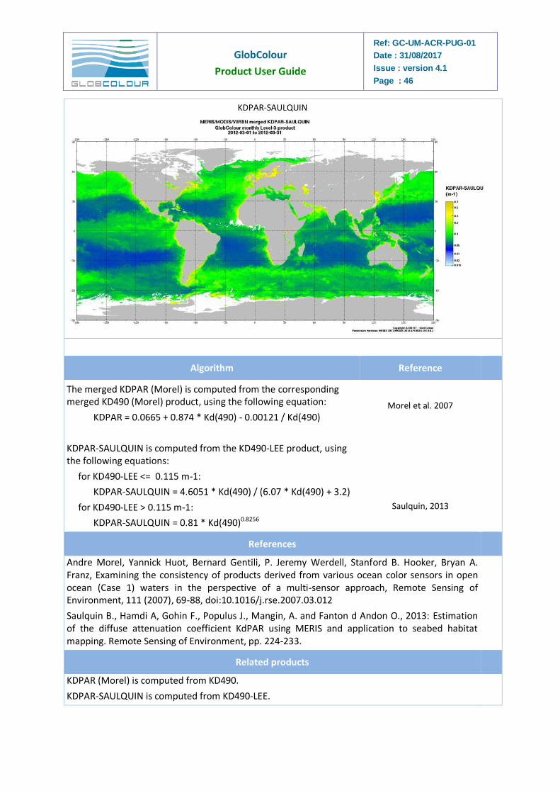
KDPAR-SAULQUIN

Algorithm Reference

The merged KDPAR (Morel) is computed from the corresponding merged KD490 (Morel) product, using the following equation:

KDPAR = 0.0665 + 0.874 * Kd(490) - 0.00121 / Kd(490)

KDPAR-SAULQUIN is computed from the KD490-LEE product, using the following equations:

for KD490-LEE <= 0.115 m-1:

KDPAR-SAULQUIN = 4.6051 * Kd(490) / (6.07 * Kd(490) + 3.2)

for KD490-LEE > 0.115 m-1:

KDPAR-SAULQUIN = 0.81 * Kd(490)0.8256

Morel et al. 2007

Saulquin, 2013

References


Saulquin B., Hamdi A, Gohin F., Populus J., Mangin, A. and Fanton d Andon O., 2013: Estimation of the diffuse attenuation coefficient KdPAR using MERIS and application to seabed habitat mapping. Remote Sensing of Environment, pp. 224-233.

Related products

KDPAR (Morel) is computed from KD490.

KDPAR-SAULQUIN is computed from KD490-LEE.

GlobColour

Product User Guide


Date : 31/08/2017

Issue : version 4.1

Page : 47

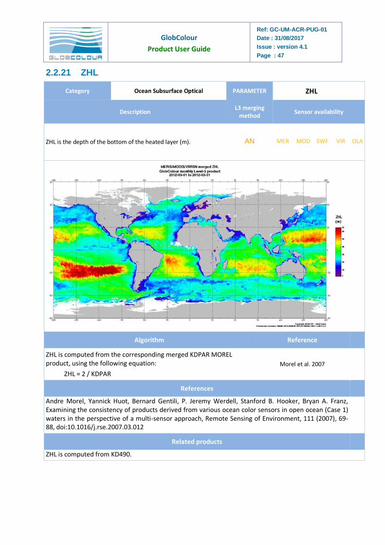
2.2.21 ZHL

Category Ocean Subsurface Optical PARAMETER ZHL



ZHL is the depth of the bottom of the heated layer (m). AN MER MOD SWF VIR OLA

Algorithm Reference

ZHL is computed from the corresponding merged KDPAR MOREL product, using the following equation:

ZHL = 2 / KDPAR

Morel et al. 2007

References


Related products

ZHL is computed from KD490.

GlobColour

Product User Guide


Date : 31/08/2017

Issue : version 4.1

Page : 48

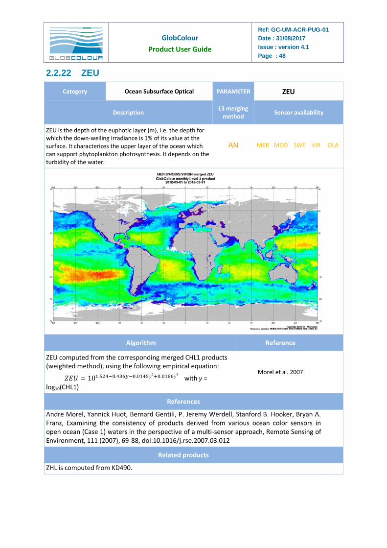
2.2.22 ZEU

Category Ocean Subsurface Optical PARAMETER ZEU



ZEU is the depth of the euphotic layer (m), i.e. the depth for which the down-welling irradiance is 1% of its value at the surface. It characterizes the upper layer of the ocean which can support phytoplankton photosynthesis. It depends on the turbidity of the water.


Algorithm Reference

ZEU computed from the corresponding merged CHL1 products (weighted method), using the following empirical equation:

𝑍𝐸𝑈 = 101.524−0.436𝑦−0.0145𝑦2+0.0186𝑦3 with y =

log10(CHL1)

Morel et al. 2007

References


Related products

ZHL is computed from KD490.

GlobColour

Product User Guide


Date : 31/08/2017

Issue : version 4.1

Page : 49

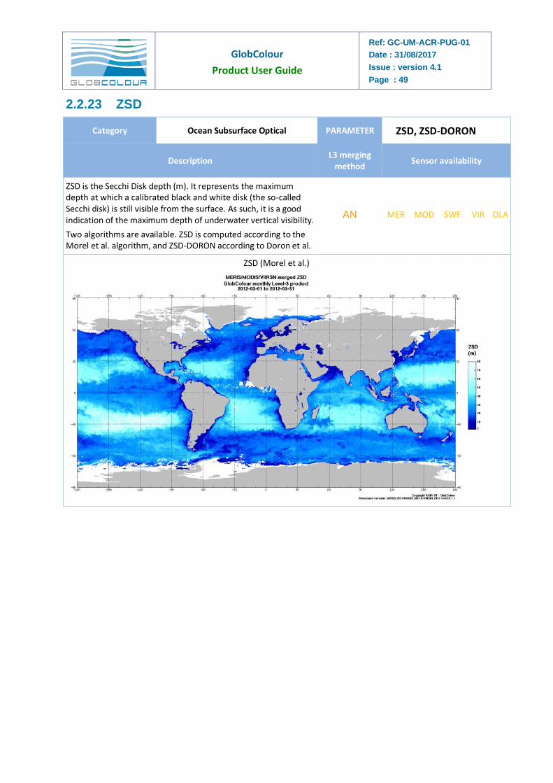
2.2.23 ZSD

Category Ocean Subsurface Optical PARAMETER ZSD, ZSD-DORON



ZSD is the Secchi Disk depth (m). It represents the maximum depth at which a calibrated black and white disk (the so-called Secchi disk) is still visible from the surface. As such, it is a good indication of the maximum depth of underwater vertical visibility.

Two algorithms are available. ZSD is computed according to the Morel et al. algorithm, and ZSD-DORON according to Doron et al.


ZSD (Morel et al.)

GlobColour

Product User Guide


Date : 31/08/2017

Issue : version 4.1

Page : 50

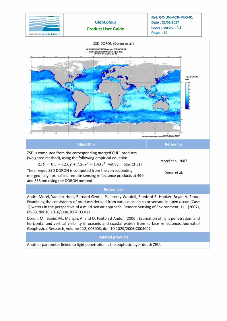
ZSD-DORON (Doron et al.)

Algorithm Reference

ZSD is computed from the corresponding merged CHL1 products (weighted method), using the following empirical equation:

𝑍𝑆𝐷 = 8.5 − 12.6𝑦 + 7.36𝑦2 − 1.43𝑦3 with y = log10(CHL1)

The merged ZSD DORON is computed from the corresponding merged fully normalised remote sensing reflectance products at 490 and 555 nm using the DORON method.

Morel et al. 2007

Doron et al.

References


Doron, M., Babin, M., Mangin, A. and O. Fanton d Andon (2006). Estimation of light penetration, and horizontal and vertical visibility in oceanic and coastal waters from surface reflectance. Journal of Geophysical Research, volume 112, C06003, doi: 10.1029/2006JC004007.

Related products

Another parameter linked to light penetration is the euphotic layer depth ZEU.

GlobColour

Product User Guide


Date : 31/08/2017

Issue : version 4.1

Page : 51

2.2.24 CHL-CIA

Category Demonstration Biochemical PARAMETER CHL-CIA



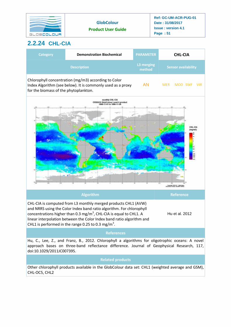
Chlorophyll concentration (mg/m3) according to Color Index Algorithm (see below). It is commonly used as a proxy for the biomass of the phytoplankton.

AN MER MOD SWF VIR

Algorithm Reference

CHL-CIA is computed from L3 monthly merged products CHL1 (AVW) and NRRS using the Color Index band ratio algorithm. For chlorophyll concentrations higher than 0.3 mg/m3, CHL-CIA is equal to CHL1. A linear interpolation between the Color Index band ratio algorithm and CHL1 is performed in the range 0.25 to 0.3 mg/m3.

Hu et al. 2012

References

Hu, C., Lee, Z., and Franz, B., 2012. Chlorophyll a algorithms for oligotrophic oceans: A novel approach bases on three-band reflectance difference. Journal of Geophysical Research, 117, doi:10.1029/2011JC007395.

Related products

Other chlorophyll products available in the GlobColour data set: CHL1 (weighted average and GSM), CHL-OC5, CHL2

GlobColour

Product User Guide


Date : 31/08/2017

Issue : version 4.1

Page : 52

2.2.25 BBPxxx-LOG

Category Demonstration Optical Subsurface PARAMETER BBPxxx-LOG



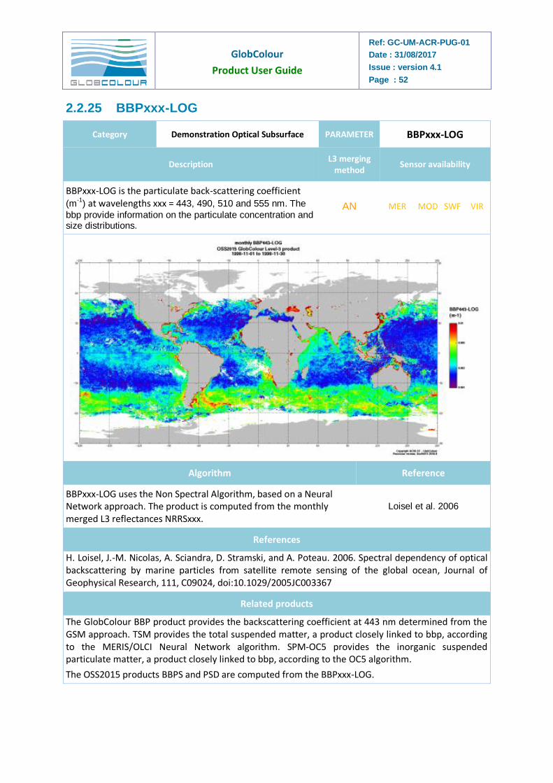
BBPxxx-LOG is the particulate back-scattering coefficient (m

-1) at wavelengths xxx = 443, 490, 510 and 555 nm. The

bbp provide information on the particulate concentration and size distributions.

AN MER MOD SWF VIR

Algorithm Reference

BBPxxx-LOG uses the Non Spectral Algorithm, based on a Neural Network approach. The product is computed from the monthly merged L3 reflectances NRRSxxx.

Loisel et al. 2006

References

H. Loisel, J.-M. Nicolas, A. Sciandra, D. Stramski, and A. Poteau. 2006. Spectral dependency of optical backscattering by marine particles from satellite remote sensing of the global ocean, Journal of Geophysical Research, 111, C09024, doi:10.1029/2005JC003367

Related products

The GlobColour BBP product provides the backscattering coefficient at 443 nm determined from the GSM approach. TSM provides the total suspended matter, a product closely linked to bbp, according to the MERIS/OLCI Neural Network algorithm. SPM-OC5 provides the inorganic suspended particulate matter, a product closely linked to bbp, according to the OC5 algorithm.

The OSS2015 products BBPS and PSD are computed from the BBPxxx-LOG.

GlobColour

Product User Guide


Date : 31/08/2017

Issue : version 4.1

Page : 53

2.2.26 BBPS-LOG

Category Demonstration Optical Subsurface PARAMETER BBPS-LOG



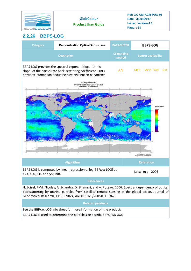
BBPS-LOG provides the spectral exponent (logarithmic slope) of the particulate back-scattering coefficient. BBPS

provides information about the size distribution of particles.

AN MER MOD SWF VIR

Algorithm Reference

BBPS-LOG is computed by linear regression of log(BBPxxx-LOG) at 443, 490, 510 and 555 nm.

Loisel et al. 2006

References


Related products

See the BBPxxx-LOG info sheet for more information on the product.

BBPS-LOG is used to determine the particle size distributions PSD-XXX

GlobColour

Product User Guide


Date : 31/08/2017

Issue : version 4.1

Page : 54

2.2.27 PSD-XXX

Category Demonstration Biochemical PARAMETER PSD-XXX



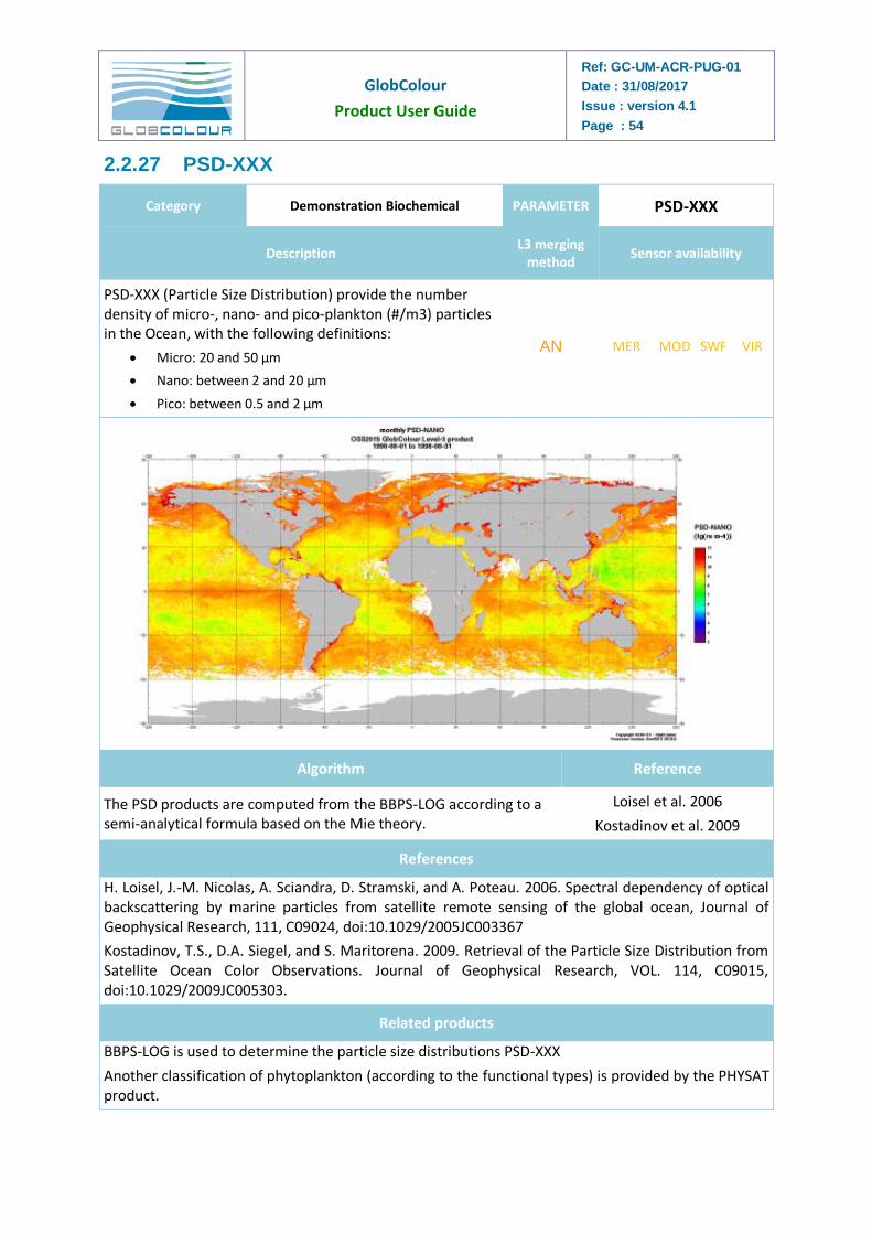
PSD-XXX (Particle Size Distribution) provide the number density of micro-, nano- and pico-plankton (#/m3) particles in the Ocean, with the following definitions:

Micro: 20 and 50 µm

Nano: between 2 and 20 µm

Pico: between 0.5 and 2 µm

AN MER MOD SWF VIR

Algorithm Reference

The PSD products are computed from the BBPS-LOG according to a semi-analytical formula based on the Mie theory.

Loisel et al. 2006

Kostadinov et al. 2009

References


Kostadinov, T.S., D.A. Siegel, and S. Maritorena. 2009. Retrieval of the Particle Size Distribution from Satellite Ocean Color Observations. Journal of Geophysical Research, VOL. 114, C09015, doi:10.1029/2009JC005303.

Related products

BBPS-LOG is used to determine the particle size distributions PSD-XXX

Another classification of phytoplankton (according to the functional types) is provided by the PHYSAT product.

GlobColour

Product User Guide


Date : 31/08/2017

Issue : version 4.1

Page : 55

2.2.28 POC-SURF

Category Demonstration Biochemical PARAMETER POC-SURF



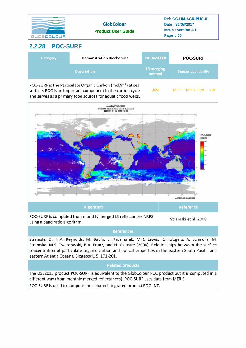
POC-SURF is the Particulate Organic Carbon (mol/m3) at sea surface. POC is an important component in the carbon cycle and serves as a primary food sources for aquatic food webs.

AN MER MOD SWF VIR

Algorithm Reference

POC-SURF is computed from monthly merged L3 reflectances NRRS using a band ratio algorithm.

Stramski et al. 2008

References

Stramski. D., R.A. Reynolds, M. Babin, S. Kaczmarek, M.R. Lewis, R. Rottgers, A. Sciandra, M. Stramska, M.S. Twardowski, B.A. Franz, and H. Claustre (2008). Relationships between the surface concentration of particulate organic carbon and optical properties in the eastern South Pacific and eastern Atlantic Oceans, Biogeosci., 5, 171-201.

Related products

The OSS2015 product POC-SURF is equivalent to the GlobColour POC product but it is computed in a different way (from monthly merged reflectances). POC-SURF uses data from MERIS.

POC-SURF is used to compute the column integrated product POC-INT.

GlobColour

Product User Guide


Date : 31/08/2017

Issue : version 4.1

Page : 56

2.2.29 POC-INT

Category Demonstration Biochemical PARAMETER POC-INT



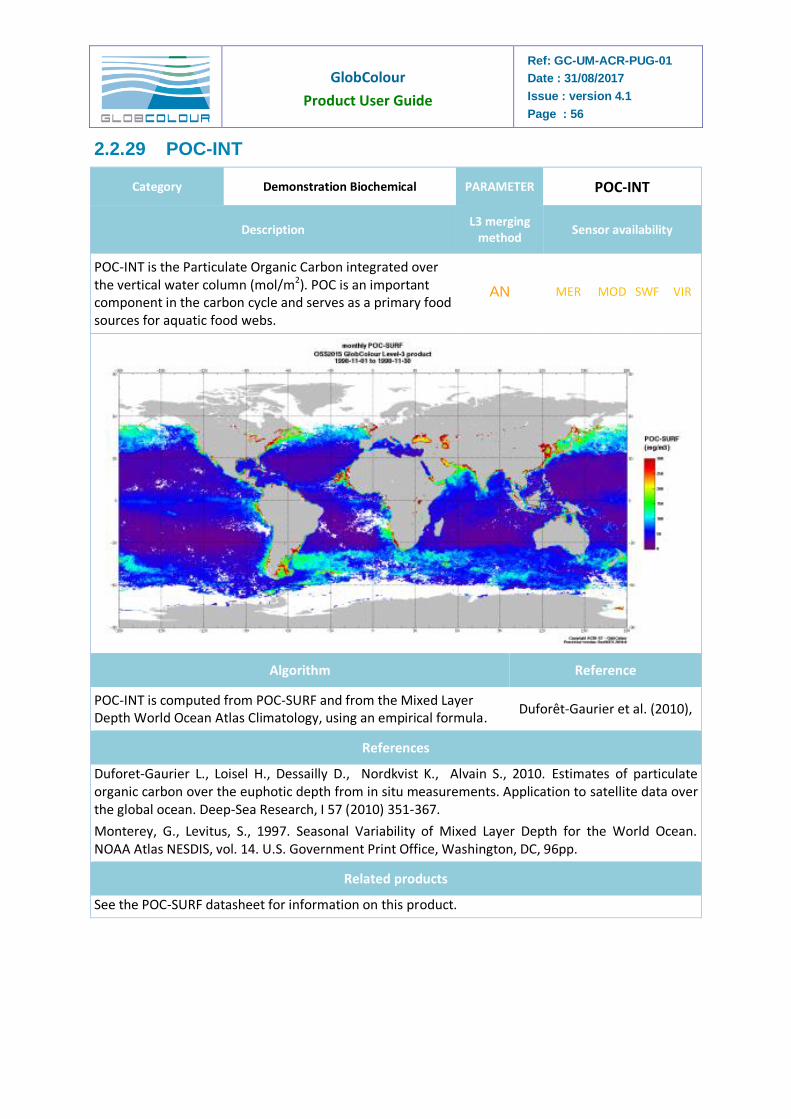
POC-INT is the Particulate Organic Carbon integrated over the vertical water column (mol/m2). POC is an important component in the carbon cycle and serves as a primary food sources for aquatic food webs.

AN MER MOD SWF VIR

Algorithm Reference

POC-INT is computed from POC-SURF and from the Mixed Layer Depth World Ocean Atlas Climatology, using an empirical formula.

Duforêt-Gaurier et al. (2010),

References

Duforet-Gaurier L., Loisel H., Dessailly D., Nordkvist K., Alvain S., 2010. Estimates of particulate organic carbon over the euphotic depth from in situ measurements. Application to satellite data over the global ocean. Deep-Sea Research, I 57 (2010) 351-367.

Monterey, G., Levitus, S., 1997. Seasonal Variability of Mixed Layer Depth for the World Ocean. NOAA Atlas NESDIS, vol. 14. U.S. Government Print Office, Washington, DC, 96pp.

Related products

See the POC-SURF datasheet for information on this product.

GlobColour

Product User Guide


Date : 31/08/2017

Issue : version 4.1

Page : 57

2.2.30 PP-AM, PP-UITZ

Category Demonstration Biochemical PARAMETER PP-AM, PP-UITZ



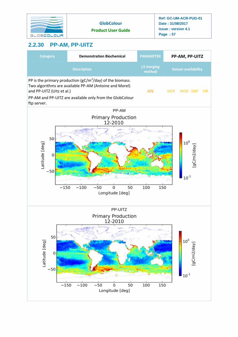
PP is the primary production (gC/m2/day) of the biomass. Two algorithms are available PP-AM (Antoine and Morel) and PP-UITZ (Uitz et al.)

PP-AM and PP-UITZ are available only from the GlobColour ftp server.

AN MER MOD SWF VIR

PP-AM

PP-UITZ

GlobColour

Product User Guide


Date : 31/08/2017

Issue : version 4.1

Page : 58

Algorithm Reference

PP-AM and PP-UITZ are computed from merged monthly L3 products using the respective algorithms.

Antoine and Morel 1996

Uitz et al. 2008

References

Antoine D. and A. Morel (1996). Oceanic primary production: 1. Adaptation of a spectral light-photosynthesis model in view of application to satellite chlorophyll observations. Global Biogeochemical Cycles, 10: 43-55

Uitz J., Y. Huot, F. Bruyant, M. Babin, and H. Claustre (2008). Relating phytoplankton photophysiological properties to community structure on large scales. Limnology and Oceanography, 53: 614\u2013630

GlobColour

Product User Guide


Date : 31/08/2017

Issue : version 4.1

Page : 59

2.2.31 PHYSAT

Category Demonstration Biochemical PARAMETER PHYSAT

Description

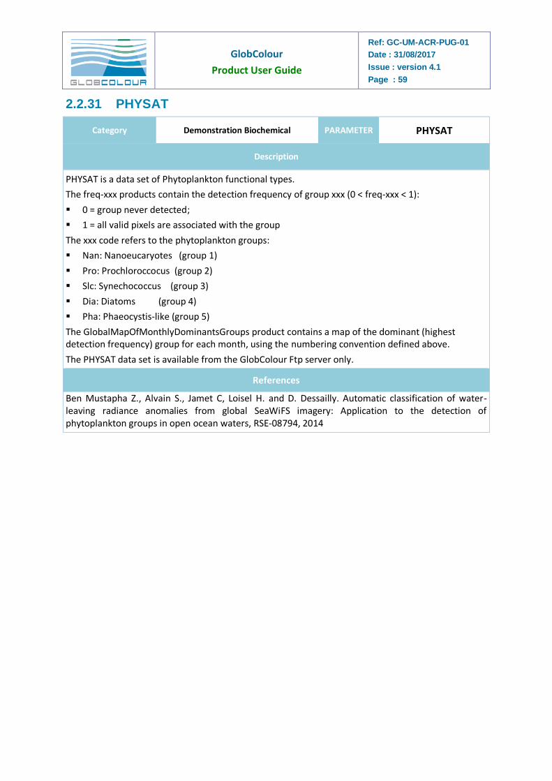
PHYSAT is a data set of Phytoplankton functional types.

The freq-xxx products contain the detection frequency of group xxx (0 < freq-xxx < 1):

0 = group never detected;

1 = all valid pixels are associated with the group

The xxx code refers to the phytoplankton groups:

Nan: Nanoeucaryotes (group 1)

Pro: Prochloroccocus (group 2)

Slc: Synechococcus (group 3)

Dia: Diatoms (group 4)

Pha: Phaeocystis-like (group 5)

The GlobalMapOfMonthlyDominantsGroups product contains a map of the dominant (highest detection frequency) group for each month, using the numbering convention defined above.

The PHYSAT data set is available from the GlobColour Ftp server only.

References

Ben Mustapha Z., Alvain S., Jamet C, Loisel H. and D. Dessailly. Automatic classification of water-leaving radiance anomalies from global SeaWiFS imagery: Application to the detection of phytoplankton groups in open ocean waters, RSE-08794, 2014

GlobColour

Product User Guide


Date : 31/08/2017

Issue : version 4.1

Page : 60

2.3 The spatial and temporal coverage

2.3.1 The binned products

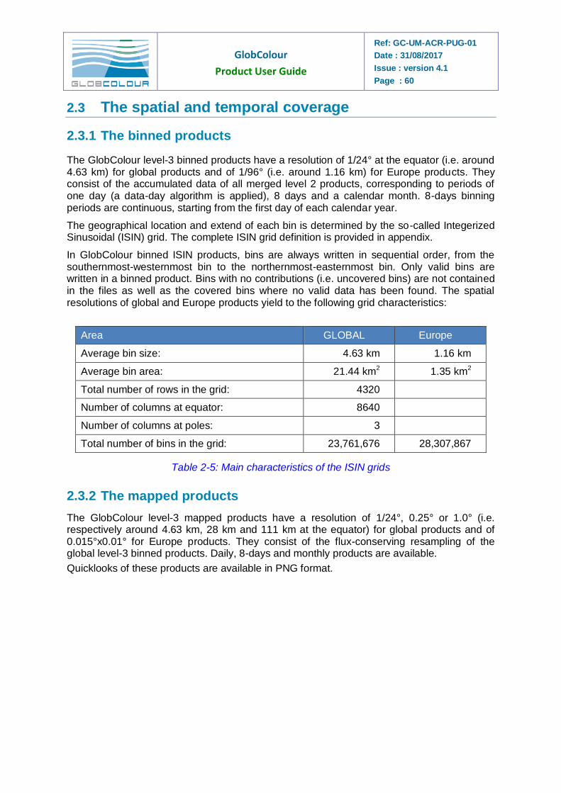
The GlobColour level-3 binned products have a resolution of 1/24° at the equator (i.e. around 4.63 km) for global products and of 1/96° (i.e. around 1.16 km) for Europe products. They consist of the accumulated data of all merged level 2 products, corresponding to periods of one day (a data-day algorithm is applied), 8 days and a calendar month. 8-days binning periods are continuous, starting from the first day of each calendar year.

The geographical location and extend of each bin is determined by the so-called Integerized Sinusoidal (ISIN) grid. The complete ISIN grid definition is provided in appendix.

In GlobColour binned ISIN products, bins are always written in sequential order, from the southernmost-westernmost bin to the northernmost-easternmost bin. Only valid bins are written in a binned product. Bins with no contributions (i.e. uncovered bins) are not contained in the files as well as the covered bins where no valid data has been found. The spatial resolutions of global and Europe products yield to the following grid characteristics:

Area GLOBAL Europe

Average bin size: 4.63 km 1.16 km

Average bin area: 21.44 km2 1.35 km2

Total number of rows in the grid: 4320

Number of columns at equator: 8640

Number of columns at poles: 3

Total number of bins in the grid: 23,761,676 28,307,867

Table 2-5: Main characteristics of the ISIN grids

2.3.2 The mapped products

The GlobColour level-3 mapped products have a resolution of 1/24°, 0.25° or 1.0° (i.e. respectively around 4.63 km, 28 km and 111 km at the equator) for global products and of 0.015°x0.01° for Europe products. They consist of the flux-conserving resampling of the global level-3 binned products. Daily, 8-days and monthly products are available.

Quicklooks of these products are available in PNG format.

GlobColour

Product User Guide


Date : 31/08/2017

Issue : version 4.1

Page : 61

3 The GlobColour system

3.1 Overall description of the processor

The GlobColour processor is the computation element of the GlobColour processing system. Its function is the transformation of EO level 2 products (or level 3 products) from independent instrument/missions into a single merged level 3 product.

The level-2 products are transformed after the sensor-specific preprocessing to the global and Europe ISIN grids. This binning is separately applied to each level-2 input product for each instrument. Outputs are intermediate spatially binned level-3 products for each instrument, also called level 3 at track level.

The term binning refers to the process of distributing the contributions of the level-2 pixels in satellite coordinates to a fixed level-3 grid using a geographic reference system.

When images of different resolutions are to be accumulated together, if the spatial coverage of each pixel is not taken into account, the importance of the image of the highest resolution are largely predominant over the images of smaller resolutions; this may result in introducing a bias in the final product.

Computing a flux value associated to each pixel may solve that problem. Assuming that the data flux for each input pixel is constant, the resampling problem is actually reduced to the problem of finding the set of pixels overlapping each level-3 bin, and then calculating the relative overlapped area.

This approach not only allows to properly mix data of various resolutions together, it also allows to distribute data properly among different level-3 bins as the input image pixel is usually overlapping several of them. This also makes it possible to produce level-3 data at a higher resolution than the input data with no "holes".

Though very attractive, the major drawback to this method is that it is significantly slower than the usual method; different techniques are being investigated to increase the speed of this approach.

The algorithm implemented in the GlobColour processing chain uses the fast Sutherland-Hodgeman area clipping. For more information on the algorithm used refer to ["A fast flux-conserving resampling algorithm", available at http://skyview.gsfc.nasa.gov/polysamp/].

The same binning algorithm is applied to each kind of input variables. Only the flags taken into account when filtering the data are different. These flags are listed in the next sub-section.

Following this logic, the GlobColour processor is mainly composed of 4 separate modules, namely:

1. a preprocessor module

2. a spatial binning module

3. a merging module

4. a temporal binning module

For each sensor, a pre-processing is foreseen just after extraction of the L2. This preprocessor serves for example in the case of MERIS/OLCI and wherever requested to transform the L2 normalised water leaving reflectances into fully normalised remote sensing

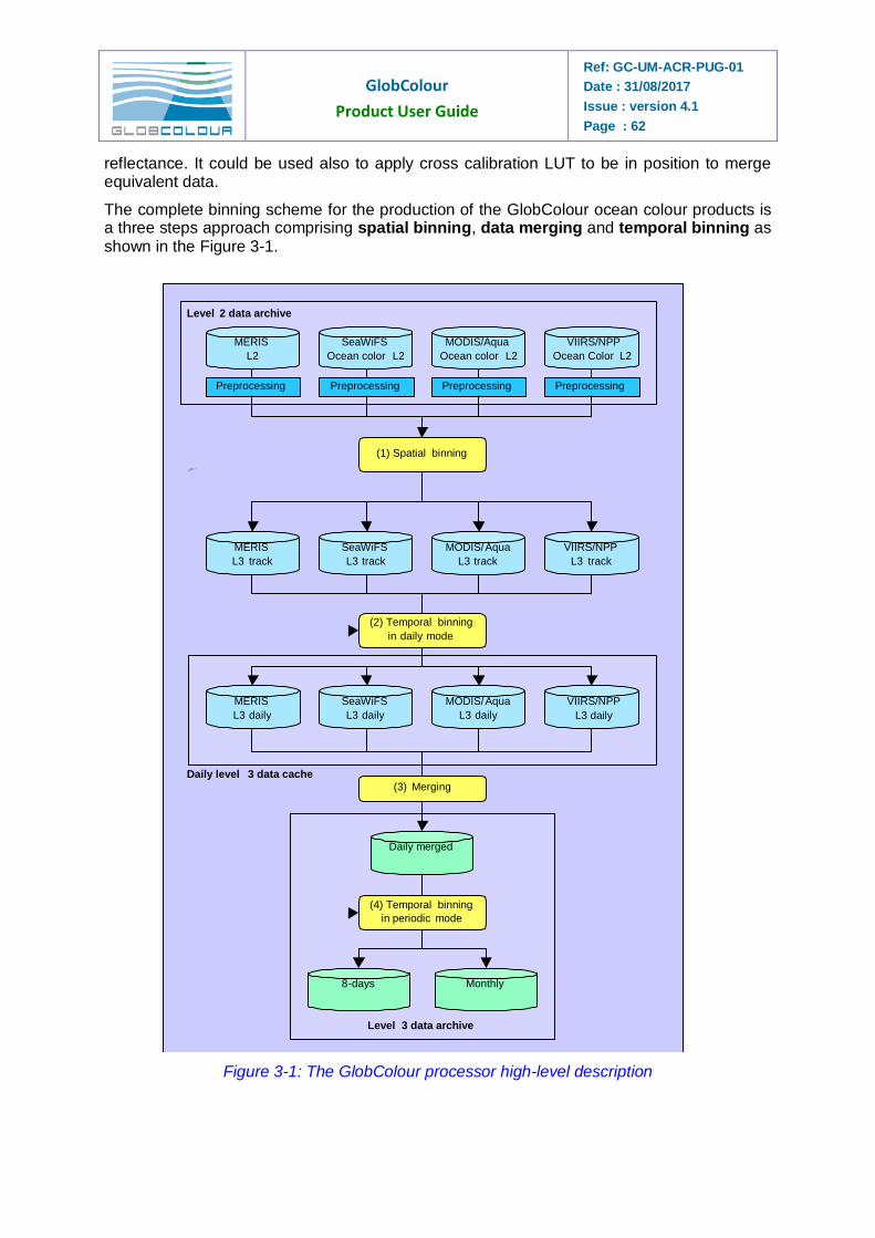
http://skyview.gsfc.nasa.gov/polysamp/

GlobColour

Product User Guide


Date : 31/08/2017

Issue : version 4.1

Page : 62

reflectance. It could be used also to apply cross calibration LUT to be in position to merge equivalent data.

The complete binning scheme for the production of the GlobColour ocean colour products is a three steps approach comprising spatial binning, data merging and temporal binning as shown in the Figure 3-1.

MERIS L2

SeaWiFS Ocean color L2

MODIS/Aqua Ocean color L2

VIIRS/NPP Ocean Color L2

Preprocessing Preprocessing Preprocessing Preprocessing

(1) Spatial binning

(2) Temporal binning in daily mode

(3) Merging

(4) Temporal binning in periodic mode

MERIS L3 track

SeaWiFS L3 track

MODIS/ Aqua L3 track

VIIRS/NPP L3 track

MERIS L3 daily

SeaWiFS L3 daily

MODIS/ Aqua L3 daily

VIIRS/NPP L3 daily

Daily merged

8 - days Monthly

Level 3 data archive

Level 2 data archive

Daily level 3 data cache

Figure 3-1: The GlobColour processor high-level description

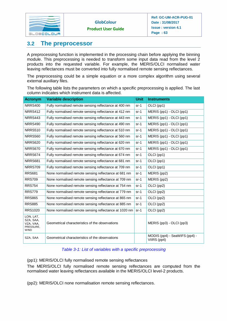
GlobColour

Product User Guide


Date : 31/08/2017

Issue : version 4.1

Page : 63

3.2 The preprocessor

A preprocessing function is implemented in the processing chain before applying the binning module. This preprocessing is needed to transform some input data read from the level 2 products into the requested variable. For example, the MERIS/OLCI normalised water leaving reflectances must be converted into fully normalised remote sensing reflectances.

The preprocessing could be a simple equation or a more complex algorithm using several external auxiliary files.

The following table lists the parameters on which a specific preprocessing is applied. The last column indicates which instrument data is affected.

Acronym Variable description Unit Instruments

NRRS400 Fully normalised remote sensing reflectance at 400 nm sr-1 OLCI (pp1)

NRRS412 Fully normalised remote sensing reflectance at 412 nm sr-1 MERIS (pp1) - OLCI (pp1)










RRS681 None normalised remote sensing reflectance at 681 nm sr-1 MERIS (pp2)

RRS709 None normalised remote sensing reflectance at 709 nm sr-1 MERIS (pp2)

RRS754 None normalised remote sensing reflectance at 754 nm sr-1 OLCI (pp2)





LON, LAT, SZA, SAA,

VZA, VAA, PRESSURE, WIND

Geometrical characteristics of the observations MERIS (pp3) - OLCI (pp3)

SZA, SAA Geometrical characteristics of the observations MODIS (pp4) - SeaWiFS (pp4) - VIIRS (pp4)

Table 3-1: List of variables with a specific preprocessing

(pp1): MERIS/OLCI fully normalised remote sensing reflectances

The MERIS/OLCI fully normalised remote sensing relfectances are computed from the normalised water leaving reflectances available in the MERIS/OLCI level-2 products.

(pp2): MERIS/OLCI none normalisation remote sensing reflectances.

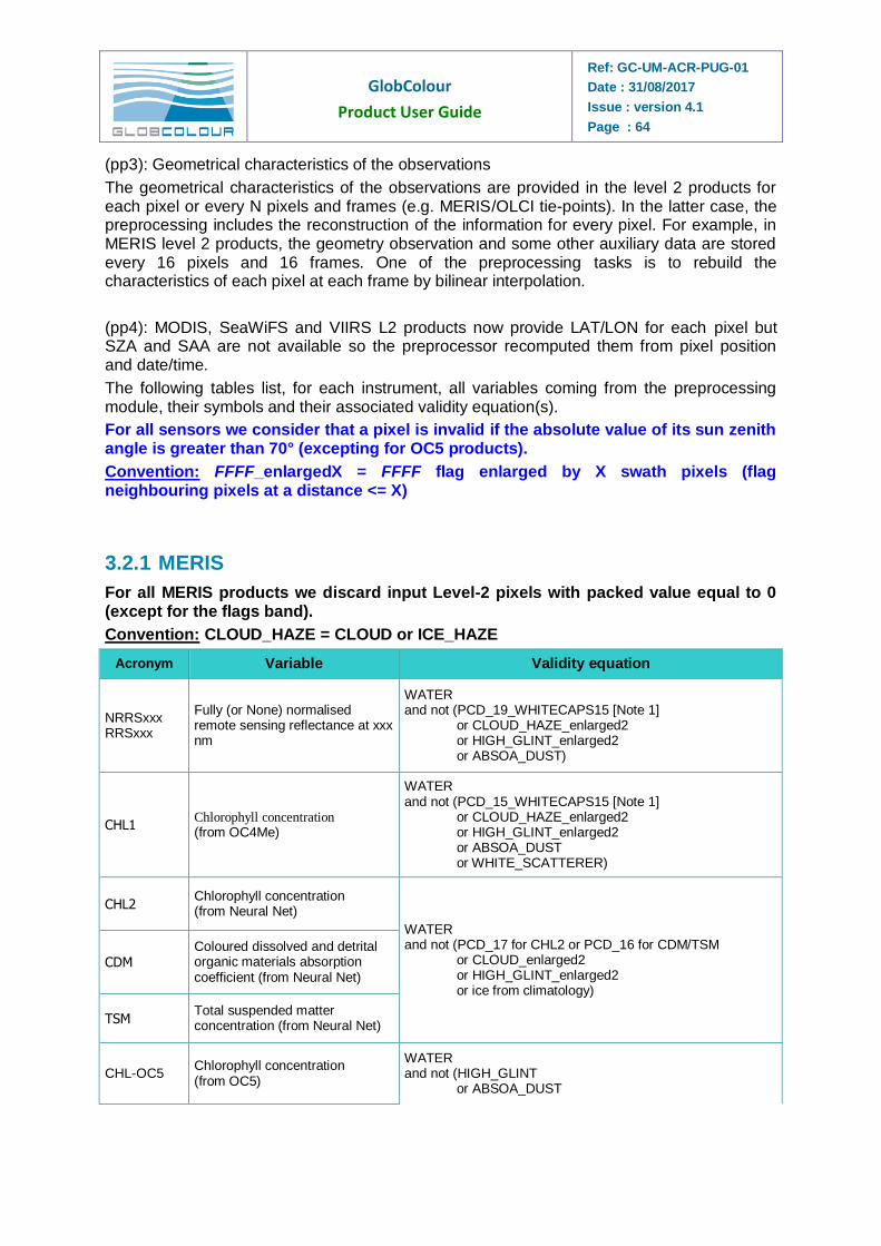
GlobColour

Product User Guide


Date : 31/08/2017

Issue : version 4.1

Page : 64

(pp3): Geometrical characteristics of the observations

The geometrical characteristics of the observations are provided in the level 2 products for each pixel or every N pixels and frames (e.g. MERIS/OLCI tie-points). In the latter case, the preprocessing includes the reconstruction of the information for every pixel. For example, in MERIS level 2 products, the geometry observation and some other auxiliary data are stored every 16 pixels and 16 frames. One of the preprocessing tasks is to rebuild the characteristics of each pixel at each frame by bilinear interpolation.

(pp4): MODIS, SeaWiFS and VIIRS L2 products now provide LAT/LON for each pixel but SZA and SAA are not available so the preprocessor recomputed them from pixel position and date/time.

The following tables list, for each instrument, all variables coming from the preprocessing module, their symbols and their associated validity equation(s).

For all sensors we consider that a pixel is invalid if the absolute value of its sun zenith angle is greater than 70° (excepting for OC5 products).

Convention: FFFF_enlargedX = FFFF flag enlarged by X swath pixels (flag neighbouring pixels at a distance <= X)

3.2.1 MERIS

For all MERIS products we discard input Level-2 pixels with packed value equal to 0 (except for the flags band).

Convention: CLOUD_HAZE = CLOUD or ICE_HAZE

Acronym Variable Validity equation

NRRSxxx RRSxxx

Fully (or None) normalised remote sensing reflectance at xxx nm

WATER and not (PCD_19_WHITECAPS15 [Note 1] or CLOUD_HAZE_enlarged2 or HIGH_GLINT_enlarged2 or ABSOA_DUST)

CHL1 Chlorophyll concentration (from OC4Me)

WATER and not (PCD_15_WHITECAPS15 [Note 1] or CLOUD_HAZE_enlarged2 or HIGH_GLINT_enlarged2 or ABSOA_DUST or WHITE_SCATTERER)

CHL2 Chlorophyll concentration (from Neural Net)

WATER and not (PCD_17 for CHL2 or PCD_16 for CDM/TSM or CLOUD_enlarged2 or HIGH_GLINT_enlarged2 or ice from climatology)

CDM Coloured dissolved and detrital organic materials absorption coefficient (from Neural Net)

TSM Total suspended matter concentration (from Neural Net)

CHL-OC5 Chlorophyll concentration (from OC5)

WATER and not (HIGH_GLINT or ABSOA_DUST

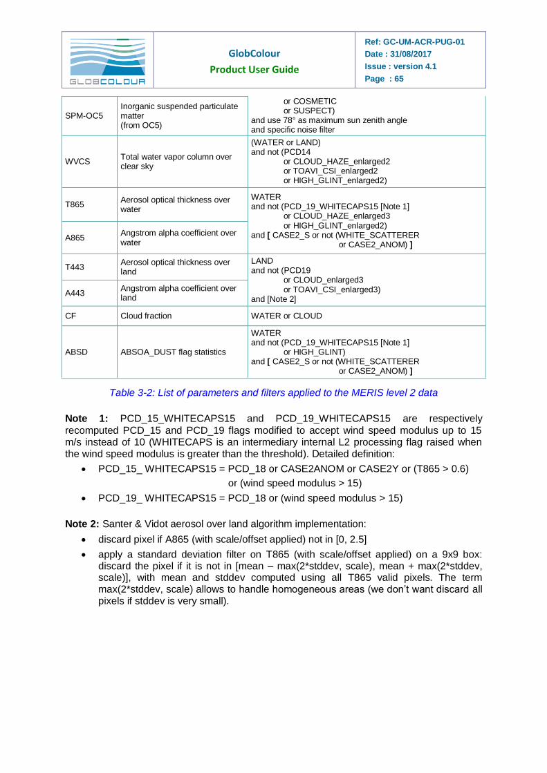
GlobColour

Product User Guide


Date : 31/08/2017

Issue : version 4.1

Page : 65

SPM-OC5 Inorganic suspended particulate matter (from OC5)

or COSMETIC or SUSPECT) and use 78° as maximum sun zenith angle and specific noise filter

WVCS Total water vapor column over clear sky

(WATER or LAND) and not (PCD14 or CLOUD_HAZE_enlarged2 or TOAVI_CSI_enlarged2 or HIGH_GLINT_enlarged2)


WATER and not (PCD_19_WHITECAPS15 [Note 1] or CLOUD_HAZE_enlarged3 or HIGH_GLINT_enlarged2) and [ CASE2_S or not (WHITE_SCATTERER or CASE2_ANOM) ]

A865 Angstrom alpha coefficient over water

T443 Aerosol optical thickness over land

LAND and not (PCD19 or CLOUD_enlarged3 or TOAVI_CSI_enlarged3) and [Note 2]

A443 Angstrom alpha coefficient over land

CF Cloud fraction WATER or CLOUD

ABSD ABSOA_DUST flag statistics

WATER and not (PCD_19_WHITECAPS15 [Note 1] or HIGH_GLINT) and [ CASE2_S or not (WHITE_SCATTERER or CASE2_ANOM) ]

Table 3-2: List of parameters and filters applied to the MERIS level 2 data

Note 1: PCD_15_WHITECAPS15 and PCD_19_WHITECAPS15 are respectively

recomputed PCD_15 and PCD_19 flags modified to accept wind speed modulus up to 15 m/s instead of 10 (WHITECAPS is an intermediary internal L2 processing flag raised when the wind speed modulus is greater than the threshold). Detailed definition:

PCD_15_ WHITECAPS15 = PCD_18 or CASE2ANOM or CASE2Y or (T865 > 0.6)

or (wind speed modulus > 15)

PCD_19_ WHITECAPS15 = PCD_18 or (wind speed modulus > 15)

Note 2: Santer & Vidot aerosol over land algorithm implementation:

discard pixel if A865 (with scale/offset applied) not in [0, 2.5]

apply a standard deviation filter on T865 (with scale/offset applied) on a 9x9 box: discard the pixel if it is not in [mean – max(2*stddev, scale), mean + max(2*stddev, scale)], with mean and stddev computed using all T865 valid pixels. The term max(2*stddev, scale) allows to handle homogeneous areas (we don’t want discard all pixels if stddev is very small).

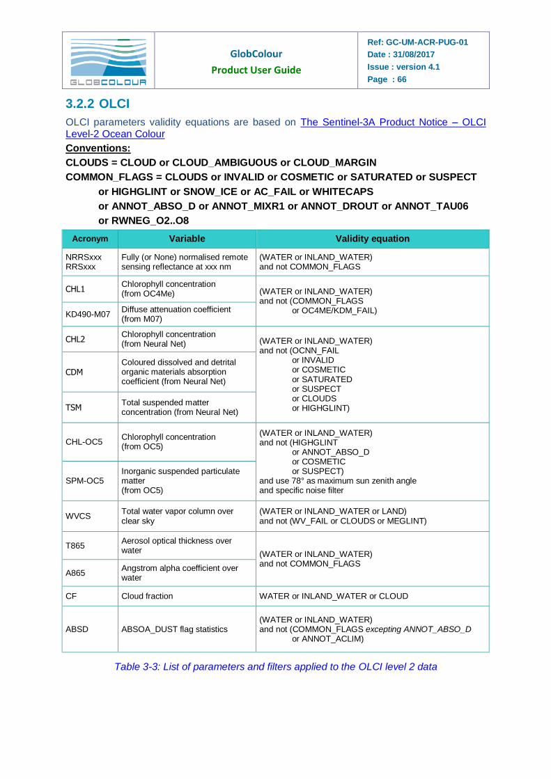
GlobColour

Product User Guide


Date : 31/08/2017

Issue : version 4.1

Page : 66

3.2.2 OLCI

OLCI parameters validity equations are based on The Sentinel-3A Product Notice – OLCI Level-2 Ocean Colour

Conventions:

CLOUDS = CLOUD or CLOUD_AMBIGUOUS or CLOUD_MARGIN

COMMON_FLAGS = CLOUDS or INVALID or COSMETIC or SATURATED or SUSPECT

or HIGHGLINT or SNOW_ICE or AC_FAIL or WHITECAPS

or ANNOT_ABSO_D or ANNOT_MIXR1 or ANNOT_DROUT or ANNOT_TAU06

or RWNEG_O2..O8


NRRSxxx RRSxxx

Fully (or None) normalised remote sensing reflectance at xxx nm

(WATER or INLAND_WATER) and not COMMON_FLAGS

CHL1 Chlorophyll concentration (from OC4Me) (WATER or INLAND_WATER)

and not (COMMON_FLAGS or OC4ME/KDM_FAIL) KD490-M07

Diffuse attenuation coefficient (from M07)

CHL2 Chlorophyll concentration (from Neural Net) (WATER or INLAND_WATER)

and not (OCNN_FAIL or INVALID or COSMETIC or SATURATED or SUSPECT or CLOUDS or HIGHGLINT)

CDM Coloured dissolved and detrital organic materials absorption coefficient (from Neural Net)

TSM Total suspended matter concentration (from Neural Net)


(WATER or INLAND_WATER) and not (HIGHGLINT or ANNOT_ABSO_D or COSMETIC or SUSPECT) and use 78° as maximum sun zenith angle and specific noise filter

SPM-OC5 Inorganic suspended particulate matter (from OC5)

WVCS Total water vapor column over clear sky

(WATER or INLAND_WATER or LAND) and not (WV_FAIL or CLOUDS or MEGLINT)

T865 Aerosol optical thickness over water (WATER or INLAND_WATER)

and not COMMON_FLAGS A865

Angstrom alpha coefficient over water

CF Cloud fraction WATER or INLAND_WATER or CLOUD

ABSD ABSOA_DUST flag statistics (WATER or INLAND_WATER) and not (COMMON_FLAGS excepting ANNOT_ABSO_D or ANNOT_ACLIM)

Table 3-3: List of parameters and filters applied to the OLCI level 2 data



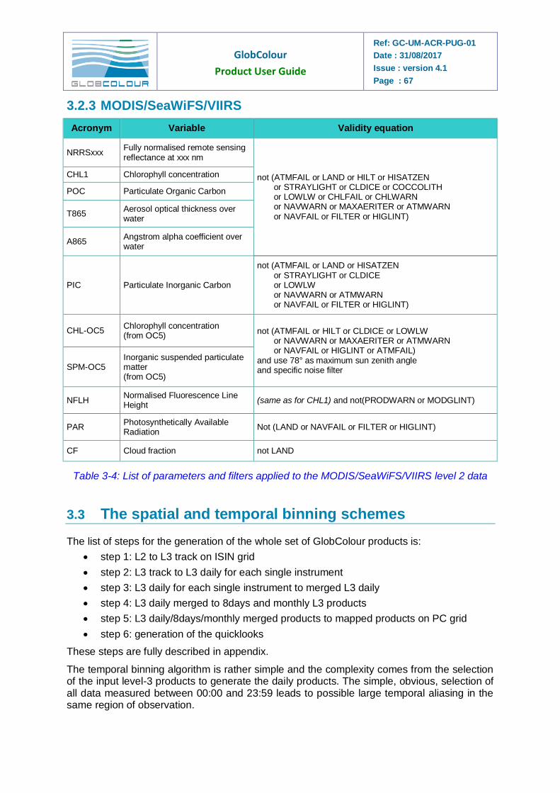
GlobColour

Product User Guide


Date : 31/08/2017

Issue : version 4.1

Page : 67

3.2.3 MODIS/SeaWiFS/VIIRS


NRRSxxx Fully normalised remote sensing reflectance at xxx nm

not (ATMFAIL or LAND or HILT or HISATZEN or STRAYLIGHT or CLDICE or COCCOLITH or LOWLW or CHLFAIL or CHLWARN or NAVWARN or MAXAERITER or ATMWARN or NAVFAIL or FILTER or HIGLINT)

CHL1 Chlorophyll concentration

POC Particulate Organic Carbon


A865 Angstrom alpha coefficient over water

PIC Particulate Inorganic Carbon

not (ATMFAIL or LAND or HISATZEN or STRAYLIGHT or CLDICE or LOWLW or NAVWARN or ATMWARN or NAVFAIL or FILTER or HIGLINT)


not (ATMFAIL or HILT or CLDICE or LOWLW or NAVWARN or MAXAERITER or ATMWARN or NAVFAIL or HIGLINT or ATMFAIL) and use 78° as maximum sun zenith angle and specific noise filter SPM-OC5

Inorganic suspended particulate matter (from OC5)

NFLH Normalised Fluorescence Line Height

(same as for CHL1) and not(PRODWARN or MODGLINT)

PAR Photosynthetically Available Radiation

Not (LAND or NAVFAIL or FILTER or HIGLINT)

CF Cloud fraction not LAND

Table 3-4: List of parameters and filters applied to the MODIS/SeaWiFS/VIIRS level 2 data

3.3 The spatial and temporal binning schemes

The list of steps for the generation of the whole set of GlobColour products is:

step 1: L2 to L3 track on ISIN grid

step 2: L3 track to L3 daily for each single instrument

step 3: L3 daily for each single instrument to merged L3 daily

step 4: L3 daily merged to 8days and monthly L3 products

step 5: L3 daily/8days/monthly merged products to mapped products on PC grid

step 6: generation of the quicklooks

These steps are fully described in appendix.

The temporal binning algorithm is rather simple and the complexity comes from the selection of the input level-3 products to generate the daily products. The simple, obvious, selection of all data measured between 00:00 and 23:59 leads to possible large temporal aliasing in the same region of observation.

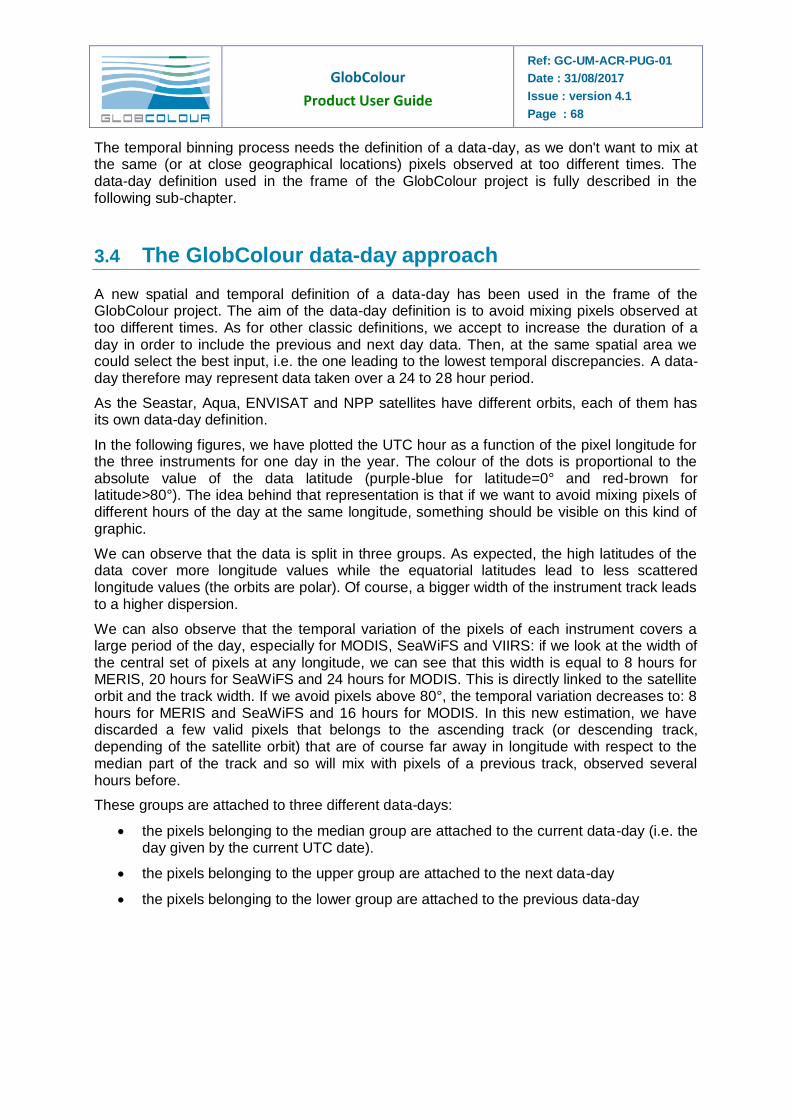
GlobColour

Product User Guide


Date : 31/08/2017

Issue : version 4.1

Page : 68

The temporal binning process needs the definition of a data-day, as we don't want to mix at the same (or at close geographical locations) pixels observed at too different times. The data-day definition used in the frame of the GlobColour project is fully described in the following sub-chapter.

3.4 The GlobColour data-day approach

A new spatial and temporal definition of a data-day has been used in the frame of the GlobColour project. The aim of the data-day definition is to avoid mixing pixels observed at too different times. As for other classic definitions, we accept to increase the duration of a day in order to include the previous and next day data. Then, at the same spatial area we could select the best input, i.e. the one leading to the lowest temporal discrepancies. A data-day therefore may represent data taken over a 24 to 28 hour period.

As the Seastar, Aqua, ENVISAT and NPP satellites have different orbits, each of them has its own data-day definition.

In the following figures, we have plotted the UTC hour as a function of the pixel longitude for the three instruments for one day in the year. The colour of the dots is proportional to the absolute value of the data latitude (purple-blue for latitude=0° and red-brown for latitude>80°). The idea behind that representation is that if we want to avoid mixing pixels of different hours of the day at the same longitude, something should be visible on this kind of graphic.

We can observe that the data is split in three groups. As expected, the high latitudes of the data cover more longitude values while the equatorial latitudes lead to less scattered longitude values (the orbits are polar). Of course, a bigger width of the instrument track leads to a higher dispersion.

We can also observe that the temporal variation of the pixels of each instrument covers a large period of the day, especially for MODIS, SeaWiFS and VIIRS: if we look at the width of the central set of pixels at any longitude, we can see that this width is equal to 8 hours for MERIS, 20 hours for SeaWiFS and 24 hours for MODIS. This is directly linked to the satellite orbit and the track width. If we avoid pixels above 80°, the temporal variation decreases to: 8 hours for MERIS and SeaWiFS and 16 hours for MODIS. In this new estimation, we have discarded a few valid pixels that belongs to the ascending track (or descending track, depending of the satellite orbit) that are of course far away in longitude with respect to the median part of the track and so will mix with pixels of a previous track, observed several hours before.

These groups are attached to three different data-days:

the pixels belonging to the median group are attached to the current data-day (i.e. the day given by the current UTC date).

the pixels belonging to the upper group are attached to the next data-day

the pixels belonging to the lower group are attached to the previous data-day

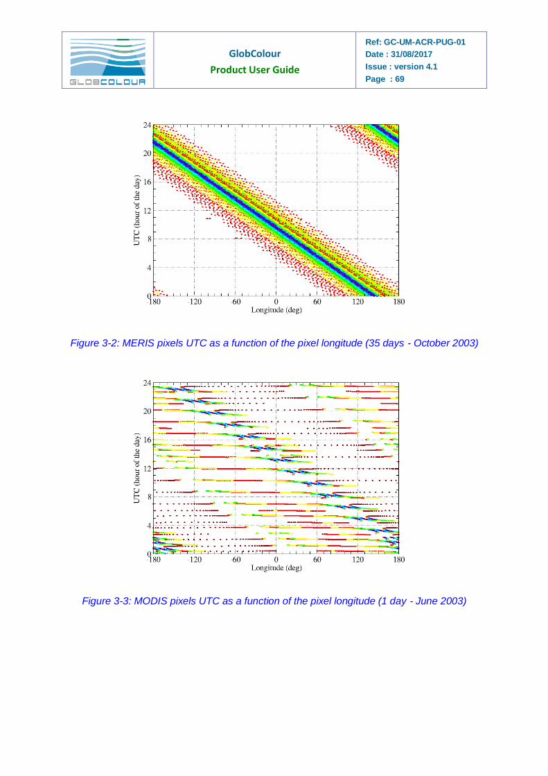
GlobColour

Product User Guide


Date : 31/08/2017

Issue : version 4.1

Page : 69

Figure 3-2: MERIS pixels UTC as a function of the pixel longitude (35 days - October 2003)

Figure 3-3: MODIS pixels UTC as a function of the pixel longitude (1 day - June 2003)

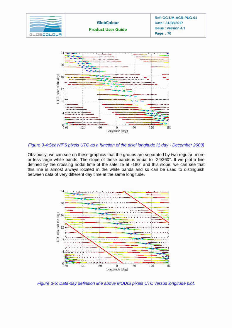
GlobColour

Product User Guide


Date : 31/08/2017

Issue : version 4.1

Page : 70

Figure 3-4:SeaWiFS pixels UTC as a function of the pixel longitude (1 day - December 2003)

Obviously, we can see on these graphics that the groups are separated by two regular, more or less large white bands. The slope of these bands is equal to -24/360°. If we plot a line defined by the crossing nodal time of the satellite at -180° and this slope, we can see that this line is almost always located in the white bands and so can be used to distinguish between data of very different day time at the same longitude.

Figure 3-5: Data-day definition line above MODIS pixels UTC versus longitude plot.

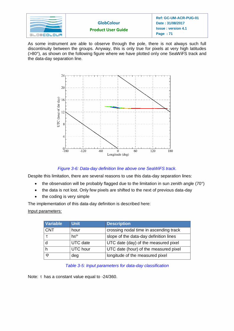
GlobColour

Product User Guide


Date : 31/08/2017

Issue : version 4.1

Page : 71

As some instrument are able to observe through the pole, there is not always such full discontinuity between the groups. Anyway, this is only true for pixels at very high latitudes (>80°), as shown on the following figure where we have plotted only one SeaWiFS track and the data-day separation line.

Figure 3-6: Data-day definition line above one SeaWiFS track.

Despite this limitation, there are several reasons to use this data-day separation lines:

the observation will be probably flagged due to the limitation in sun zenith angle (70°)

the data is not lost. Only few pixels are shifted to the next of previous data-day

the coding is very simple

The implementation of this data-day definition is described here:

Input parameters:

Variable Unit Description

CNT hour crossing nodal time in ascending track

hr/° slope of the data-day definition lines

d UTC date UTC date (day) of the measured pixel

h UTC hour UTC date (hour) of the measured pixel

deg longitude of the measured pixel

Table 3-5: Input parameters for data-day classification

Note: has a constant value equal to -24/360.

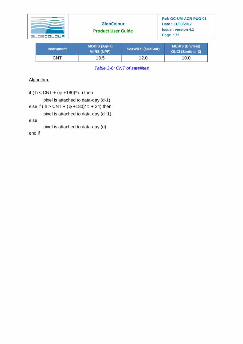
GlobColour

Product User Guide


Date : 31/08/2017

Issue : version 4.1

Page : 72

Instrument MODIS (Aqua)

VIIRS (NPP) SeaWiFS (SeaStar)

MERIS (Envisat)

OLCI (Sentinel-3)

CNT 13.5 12.0 10.0

Table 3-6: CNT of satellites

Algorithm:

if ( h < CNT + ( +180)* ) then

pixel is attached to data-day (d-1)

else if ( h > CNT + ( +180)* + 24) then

pixel is attached to data-day (d+1)

else

pixel is attached to data-day (d)

end if

GlobColour

Product User Guide


Date : 31/08/2017

Issue : version 4.1

Page : 73

4 The products format

4.1 General rules

The GlobColour Level-3 binning scheme and its output products have been designed with respect to a number of widely used definitions and de-facto standards:

- netCDF Climate and Forecast Metadata Conventions CF

- NASA Ocean Color Level-3 products

- GHRSST-PP Level-4 products

- IOCCG Report number 4

GlobColour Level-3 output data includes binned, mapped and quicklook products which are described in the following sections. The binned and mapped products are stored in netCDF-4 files. The netCDF-4 library or third-party tools including netCDF-4 readers must be used to read the GlobColour products. The quicklook products are written in PNG format.

netCDF (Network Common Data Form) is a machine-independent, self-describing, binary data format standard for exchanging scientific data. The project homepage is hosted by the Unidata program at the University Corporation for Atmospheric Research (UCAR). They are also the chief source of netCDF software, standards development, updates etc. The format is an open standard (see http://www.unidata.ucar.edu/software/netcdf).

The version 4 of the netCDF format provides new features which are used for GlobColour products: chunking and internal compression. These two features allow us to distribute files with reduced compressed size and optimized random access: reading a small window on a product needs only to read and decompress the chunks covering it, without decompressing the whole file. Other new feature of netCDF-4 like new unsigned data types and groups are not used for GlobColour products to keep compatibility with the netCDF-3 data model: existing netCDF-3 tools could be easily re-used without any other modification than re-linking the program with the version 4 of the library. Note that the netCDF-4 format is now based on the widely supported HDF5 scientific data format, which means that any HDF5 tool will be also able to read the GlobColour products.

The following rules are applied when writing the binned (ISIN grid) and mapped products (PC grid):

each parameter is stored in a single file including metadata and accumulated statistical data.

global metadata are stored as global attributes

accumulated statistical data are stored as variables

metadata related to statistical data are stored as variable attributes.

4.2 Naming convention

This naming convention is common to all GlobColour products (but not to OSS2015 third-party products). The file naming convention of the files follows the following rules:

Lzz_date_time_ROI_SR_INS_PRD_TC_nn.ext

where:

- Lzz is the product level (L3b for level 3 binned ISIN grid, L3m for level 3 mapped grid)

http://www.unidata.ucar.edu/software/netcdf

GlobColour

Product User Guide


Date : 31/08/2017

Issue : version 4.1

Page : 74

- date is specified in UTC format as yyyymmdd[-yyyymmdd]. The end date is optional for track and daily products.

- time is specified in UTC format as hhmmss[-duration]. The time field is needed only for track products. The duration is expressed in seconds.

- ROI is the name of the region of interest (e.g. GLOB for global coverage, EURO for

Europe area).

- SR indicates the resolution of the grid (e.g. 4 for 1/24° ISIN grid).

- INS is the instrument acronym (MER for MERIS, MOD for MODIS, SWF for SeaWiFS, VIR for VIIRS, OLA for OLCI-A, or any combination of these names for the merged products). For the merged products, the instrument acronym is prefixed with the merging method (AV for simple average, AVW for weighted average, GSM for the GSM model).

- PRD is the product type (CHL for chlorophyll...). Note that the various parameter algorithms can be indicated in this field using a “-“ delimiter (e.g. CHL1-OC5, KD490-LEE).

- TC is the time coverage (TR for track-level products, DAY for daily, 8D for 8days, MO for monthly).

- nn is a counter. For track products, we store in this counter the data-day in yyyymmdd

format.

- ext is the file extension (nc for netCDF files, png for PNG files)

The number of field is constant. Missing information leads to two adjacent underscores.

Examples:

L3b_20040101_072312-2363_GLOB_4_MER_NRRS555_TR_20040101.nc

L3m_20040401__EURO_1_MOD_CHL1_DAY_00.nc

L3b_20040401-20040430__GLOB_4_MER_NRRS413_MO_00.nc

L3b_20021001-20021031__GLOB_4_AV-MERMODSWF_T865_MO_00.nc

4.3 The binned products

A netCDF dataset is made up of three basic components:

dimensions

variables

variables attributes

global attributes

The variables store the actual data, the dimensions give the relevant dimension information for the variables, and the attributes provide auxiliary information about the variables or the dataset itself.

Dimensions

All variables stored in the ISIN binned product use one of the two dimensions:

GlobColour

Product User Guide


Date : 31/08/2017

Issue : version 4.1

Page : 75

Dimension Parameter Description

bin Number of bins written in the product

row Number of useful rows in the global ISIN grid (number of row between northernmost and southernmost bins)

Table 4-1: Dimensions - binned products

Variables

ISIN grid location variables (only present in ISIN case). Some variable names are prefixed by the name of the parameter (e.g. CHL1_mean, EL555_weight).

Variable Name netCDF Type Nb of bytes Parameter Description

row(bin) NC_SHORT or NC_INT (3)

2 or 4

(3)

Latitudinal band index of the bins stored in the product, zero based and beginning at south (1)

col(bin) NC_SHORT or NC_INT (3)

2 or 4

(3)

Longitudinal index of the bins stored in the product, zero based and beginning at west (1)

center_lat(row) NC_FLOAT 4 Center latitude for each useful row (1)

center_lon(row) NC_FLOAT 4 Center longitude of the first bin (the first bin in the ISIN grid, not the first valid bin) for each useful row (1)

lon_step(row) NC_FLOAT 4 Longitude step for each useful row (1)

PRM_mean(bin) NC_FLOAT 4 Average value of the binned pixels values

PRM_stdev(bin) NC_FLOAT 4 Standard deviation of the square of the binned pixels values

PRM_count(bin) NC_SHORT 2 Number of binned pixels

PRM_weight(bin) NC_FLOAT 4 Sum of the weights of the binned pixels

PRM_flags(bin) NC_SHORT 2 Flags (4)

PRM_error(bin) NC_SHORT 2 Error estimation for the geophysical variable (2)

Table 4-2: Variables - binned products

Note 1: the row(), col(), center_lat, center_lon and lon_step() arrays allow an easier conversion of the bin index into geographical coordinates rather than the global idx() array written in the SeaWiFS and MODIS level 3 products.

Equations to compute center longitude and latitude for a bin b are:

index = row(b) – first_row (first_row is a global attribute)

lat(b) = center_lat( index )

lon(b) = center_lon( index ) + col(b) * lon_step( index )

Note 2: the error associated to each bin is computed from representative values of the bin (e.g. arithmetic mean) and observation conditions (e.g. zenith angles) using a LUT read from an external auxiliary file. The error variable is stored only in products where it is significant (i.e. the error bar is not used for simple averaging merging, and so the error is of course not stored). The error bar is stored in % packed into a 2 bytes integers using a scale factor of

GlobColour

Product User Guide


Date : 31/08/2017

Issue : version 4.1

Page : 76

0.01 (this kind of data packing is standard in netCDF). The biggest error bar possible in this format is 327.67, so if a computed error bar is greater than 327.67 then it is set to 327.67.

Note 3: these variables type could be NC_SHORT or NC_INT depending on the ISIN grid resolution.

Note 4: the quality control is available through a flags array (2 bytes), provided for each bin of each product (source of instrument: all, MODIS only..., green reflectance threshold, mostly cloudy pixel, etc...). The next table contains the current flags definition. A flag is set if its bit is set to 1. The “Bit” column contains each flag bit number, from the least to the most significant bit of the 2 bytes. The flags definition is also stored in the product itself following the netCDF “CF” (Climate and Forecast) convention.

Bit Flag code Description

0 NO_MEASUREMENT Bin not covered by any L2 swaths pixel, valid or invalid (out of swaths)

1 INVALID Bin covered, but only by invalid pixel(s) (invalid because L2 flags, clouds, land, …)

2 OLCI_A OLCI(A) valid pixel(s) contribute to the bin value

3 LAND Bin covered by more than 50% of land. If not set, bin is considered as water. (1) (4)

4 CLOUD1 Cloud fraction (2)

5 CLOUD2

6 DEPTH1 Water depth (1) (3)

7 DEPTH2

8 TURBID Computed from EL555. TURBID flag is raised when EL555 is greater than 0

9 ICE Bin covered by ice. Computed from an ice climatology.

10 TROPHIC1 Trophic classification (5)

11 TROPHIC2

12 VIIRS_N VIIRS(N) valid pixel(s) contribute to the bin value

13 SEAWIFS SeaWiFS valid pixel(s) contribute to the bin value

14 MODIS MODIS valid pixel(s) contribute to the bin value

15 MERIS MERIS valid pixel(s) contribute to the bin value

Table 4-3: Flags description

Note 1: computed using a common global land elevation and ocean bathymetry product (data from ESA). This product is computed at 4.63 km on the global ISIN and PC grids.

Note 2: for 8-days or longer periods, cloud fraction flags are not yet defined (flags are currently set to 0). For daily products they define a cloud coverage classification based on the value of the CF product:

(CLOUD2=0) + (CLOUD1=0): CF < 5%

(CLOUD2=0) + (CLOUD1=1): 5% <= CF < 25%

(CLOUD2=1) + (CLOUD1=0): 25% <= CF < 50%

(CLOUD2=1) + (CLOUD1=1): CF >= 50%

Note 3: (DEPTH2=0) + (DEPTH1=0): depth < 30m

GlobColour

Product User Guide


Date : 31/08/2017

Issue : version 4.1

Page : 77

(DEPTH2=0) + (DEPTH1=1): 30m <= depth < 200m

(DEPTH2=1) + (DEPTH1=0): 200m <= depth < 1000m

(DEPTH2=1) + (DEPTH1=1): depth >= 1000m

Note 4: it is possible that a bin flagged LAND has a valid parameter value near the coastline.

Note 5: (TROPHIC2=0) + (TROPHIC1=1): Oligotrophic water

(TROPHIC2=1) + (TROPHIC1=0): Mesotrophic water

(TROPHIC2=1) + (TROPHIC1=1): Eutrophic water

Variables attributes

The following table lists the variable attributes used in the GlobColour project. These attributes are commonly used to annotate variable in netCDF files and their usage is strongly encouraged by the CF metadata conventions (excepting for pct_characterised_error which is GlobColour specific).

Attribute Name netCDF type Attribute Description

long_name string A descriptive name that indicates a variable's content. We set it to the “Parameter Description” of the previous table

standard_name string If available, a CF standard name that references a description of variable’s content

_FillValue same type as variable

A value used to indicate array elements containing no valid data

units string Text description of the physical units, preferably S.I. Some variables (row, col, count, flags, …) don’t have any units attribute

pct_characterised_error

NC_FLOAT Characterised error, expressed in %

Table 4-4: Variables attributes - binned products

Global attributes

This section presents the metadata that are written in the main product file. Metadata is stored as global attributes in the netCDF file.

General product information


Conventions string Indicates compatibility with the Climate and Forecast (CF) netCDF convention. “CF-1.4”

title string A high-level descriptive title for the product

product_name string The name of the product without path.

product_type string Temporal binning period: e.g. “track”, "day", "week", “8-day”, "month"

product_version string Version of the product format

product_level NC_SHORT Product level: 3

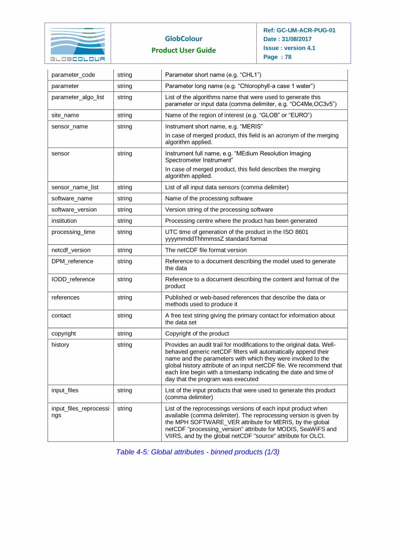
GlobColour

Product User Guide


Date : 31/08/2017

Issue : version 4.1

Page : 78

parameter_code string Parameter short name (e.g. “CHL1”)

parameter string Parameter long name (e.g. “Chlorophyll-a case 1 water”)

parameter_algo_list string List of the algorithms name that were used to generate this parameter or input data (comma delimiter, e.g. “OC4Me,OC3v5”)

site_name string Name of the region of interest (e.g. “GLOB” or “EURO”)

sensor_name string Instrument short name, e.g. “MERIS”

In case of merged product, this field is an acronym of the merging algorithm applied.

sensor string Instrument full name, e.g. “MEdium Resolution Imaging Spectrometer Instrument”

In case of merged product, this field describes the merging algorithm applied.

sensor_name_list string List of all input data sensors (comma delimiter)

software_name string Name of the processing software

software_version string Version string of the processing software

institution string Processing centre where the product has been generated

processing_time string UTC time of generation of the product in the ISO 8601 yyyymmddThhmmssZ standard format

netcdf_version string The netCDF file format version

DPM_reference string Reference to a document describing the model used to generate the data

IODD_reference string Reference to a document describing the content and format of the product

references string Published or web-based references that describe the data or methods used to produce it

contact string A free text string giving the primary contact for information about the data set

copyright string Copyright of the product

history string Provides an audit trail for modifications to the original data. Well-behaved generic netCDF filters will automatically append their name and the parameters with which they were invoked to the global history attribute of an input netCDF file. We recommend that each line begin with a timestamp indicating the date and time of day that the program was executed

input_files string List of the input products that were used to generate this product (comma delimiter)

input_files_reprocessings

string List of the reprocessings versions of each input product when available (comma delimiter). The reprocessing version is given by the MPH SOFTWARE_VER attribute for MERIS, by the global netCDF "processing_version" attribute for MODIS, SeaWiFS and VIIRS, and by the global netCDF "source" attribute for OLCI.

Table 4-5: Global attributes - binned products (1/3)

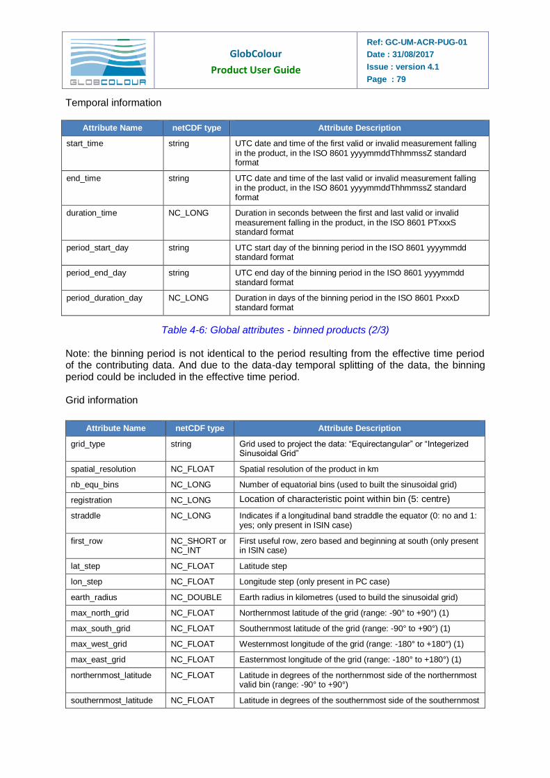
GlobColour

Product User Guide


Date : 31/08/2017

Issue : version 4.1

Page : 79

Temporal information


start_time string UTC date and time of the first valid or invalid measurement falling in the product, in the ISO 8601 yyyymmddThhmmssZ standard format

end_time string UTC date and time of the last valid or invalid measurement falling in the product, in the ISO 8601 yyyymmddThhmmssZ standard format

duration_time NC_LONG Duration in seconds between the first and last valid or invalid measurement falling in the product, in the ISO 8601 PTxxxS standard format

period_start_day string UTC start day of the binning period in the ISO 8601 yyyymmdd standard format

period_end_day string UTC end day of the binning period in the ISO 8601 yyyymmdd standard format

period_duration_day NC_LONG Duration in days of the binning period in the ISO 8601 PxxxD standard format


Note: the binning period is not identical to the period resulting from the effective time period of the contributing data. And due to the data-day temporal splitting of the data, the binning period could be included in the effective time period. Grid information


grid_type string Grid used to project the data: “Equirectangular” or “Integerized Sinusoidal Grid”

spatial_resolution NC_FLOAT Spatial resolution of the product in km

nb_equ_bins NC_LONG Number of equatorial bins (used to built the sinusoidal grid)

registration NC_LONG Location of characteristic point within bin (5: centre)

straddle NC_LONG Indicates if a longitudinal band straddle the equator (0: no and 1: yes; only present in ISIN case)

first_row NC_SHORT or NC_INT

First useful row, zero based and beginning at south (only present in ISIN case)

lat_step NC_FLOAT Latitude step

lon_step NC_FLOAT Longitude step (only present in PC case)

earth_radius NC_DOUBLE Earth radius in kilometres (used to build the sinusoidal grid)

max_north_grid NC_FLOAT Northernmost latitude of the grid (range: -90° to +90°) (1)

max_south_grid NC_FLOAT Southernmost latitude of the grid (range: -90° to +90°) (1)

max_west_grid NC_FLOAT Westernmost longitude of the grid (range: -180° to +180°) (1)

max_east_grid NC_FLOAT Easternmost longitude of the grid (range: -180° to +180°) (1)

northernmost_latitude NC_FLOAT Latitude in degrees of the northernmost side of the northernmost valid bin (range: -90° to +90°)

southernmost_latitude NC_FLOAT Latitude in degrees of the southernmost side of the southernmost

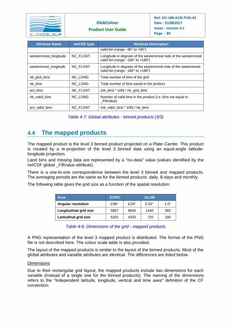
GlobColour

Product User Guide


Date : 31/08/2017

Issue : version 4.1

Page : 80


valid bin (range: -90° to +90°)

westernmost_longitude NC_FLOAT Longitude in degrees of the westernmost side of the westernmost valid bin (range: -180° to +180°)

easternmost_longitude NC_FLOAT Longitude in degrees of the easternmost side of the easternmost valid bin (range: -180° to +180°)

nb_grid_bins NC_LONG Total number of bins of the grid

nb_bins NC_LONG Total number of bins saved in the product

pct_bins NC_FLOAT (nb_bins * 100) / nb_grid_bins

nb_valid_bins NC_LONG Number of valid bins in the product (i.e. bins not equal to _FillValue)

pct_valid_bins NC_FLOAT (nb_valid_bins * 100) / nb_bins


4.4 The mapped products

The mapped product is the level 3 binned product projected on a Plate-Carrée. This product is created by a re-projection of the level 3 binned data using an equal-angle latitude-longitude projection.

Land bins and missing data are represented by a "no-data" value (values identified by the netCDF global _FillValue attribute).

There is a one-to-one correspondence between the level 3 binned and mapped products. The averaging periods are the same as for the binned products: daily, 8-days and monthly.

The following table gives the grid size as a function of the spatial resolution:

Area EURO GLOB

Angular resolution 1/96° 1/24° 0.25° 1.0°

Longitudinal grid size 5867 8640 1440 360

Latitudinal grid size 5201 4320 720 180

Table 4-8: Dimensions of the grid - mapped products

A PNG representation of the level 3 mapped product is distributed. The format of the PNG file is not described here. The colour scale table is also provided.

The layout of the mapped products is similar to the layout of the binned products. Most of the global attributes and variable attributes are identical. The differences are listed below.

Dimensions

Due to their rectangular grid layout, the mapped products include two dimensions for each variable (instead of a single one for the binned products). The naming of the dimensions refers to the "Independent latitude, longitude, vertical and time axes" definition of the CF convention.

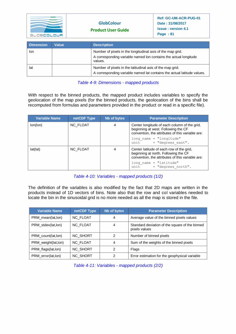
GlobColour

Product User Guide


Date : 31/08/2017

Issue : version 4.1

Page : 81

Dimension Value Description

lon Number of pixels in the longitudinal axis of the map grid.

A corresponding variable named lon contains the actual longitude values.

lat Number of pixels in the latitudinal axis of the map grid.

A corresponding variable named lat contains the actual latitude values.

Table 4-9: Dimensions - mapped products

With respect to the binned products, the mapped product includes variables to specify the geolocation of the map pixels (for the binned products, the geolocation of the bins shall be recomputed from formulas and parameters provided in the product or read in a specific file).


lon(lon) NC_FLOAT 4 Center longitude of each column of the grid, beginning at west. Following the CF convention, the attributes of this variable are:

long_name = "longitude"

unit = "degrees_east".

lat(lat) NC_FLOAT 4 Center latitude of each row of the grid, beginning at north. Following the CF convention, the attributes of this variable are:

long_name = "latitude"

unit = "degrees_north".

Table 4-10: Variables - mapped products (1/2)

The definition of the variables is also modified by the fact that 2D maps are written in the products instead of 1D vectors of bins. Note also that the row and col variables needed to locate the bin in the sinusoidal grid is no more needed as all the map is stored in the file.


PRM_mean(lat,lon) NC_FLOAT 4 Average value of the binned pixels values

PRM_stdev(lat,lon) NC_FLOAT 4 Standard deviation of the square of the binned pixels values

PRM_count(lat,lon) NC_SHORT 2 Number of binned pixels

PRM_weight(lat,lon) NC_FLOAT 4 Sum of the weights of the binned pixels

PRM_flags(lat,lon) NC_SHORT 2 Flags

PRM_error(lat,lon) NC_SHORT 2 Error estimation for the geophysical variable

Table 4-11: Variables - mapped products (2/2)

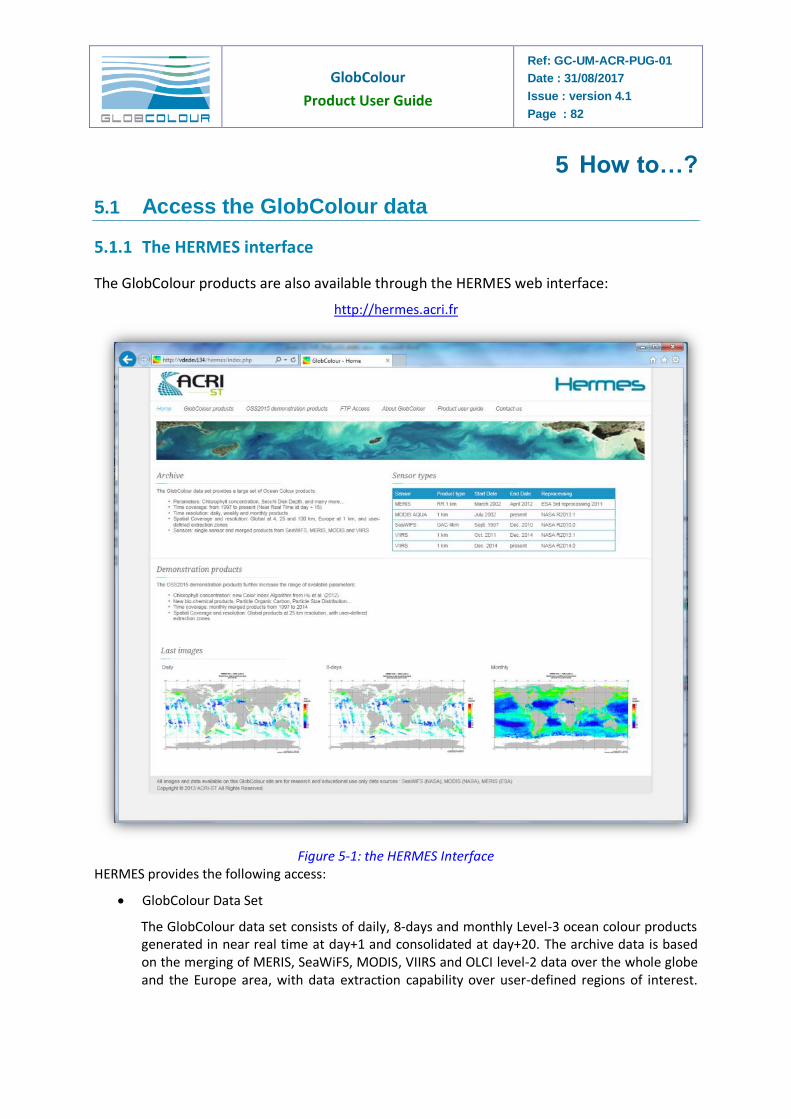
GlobColour

Product User Guide


Date : 31/08/2017

Issue : version 4.1

Page : 82

5 How to…?

5.1 Access the GlobColour data

5.1.1 The HERMES interface

The GlobColour products are also available through the HERMES web interface:

http://hermes.acri.fr

Figure 5-1: the HERMES Interface

HERMES provides the following access:

GlobColour Data Set

The GlobColour data set consists of daily, 8-days and monthly Level-3 ocean colour products generated in near real time at day+1 and consolidated at day+20. The archive data is based on the merging of MERIS, SeaWiFS, MODIS, VIIRS and OLCI level-2 data over the whole globe and the Europe area, with data extraction capability over user-defined regions of interest.

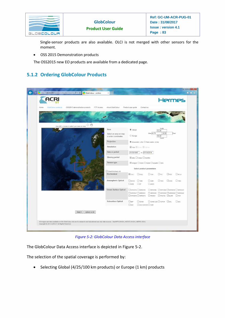
GlobColour

Product User Guide


Date : 31/08/2017

Issue : version 4.1

Page : 83

Single-sensor products are also available. OLCI is not merged with other sensors for the moment.

OSS 2015 Demonstration products

The OSS2015 new EO products are available from a dedicated page.

5.1.2 Ordering GlobColour Products

Figure 5-2: GlobColour Data Access interface

The GlobColour Data Access interface is depicted in Figure 5-2.

The selection of the spatial coverage is performed by:

Selecting Global (4/25/100 km products) or Europe (1 km) products

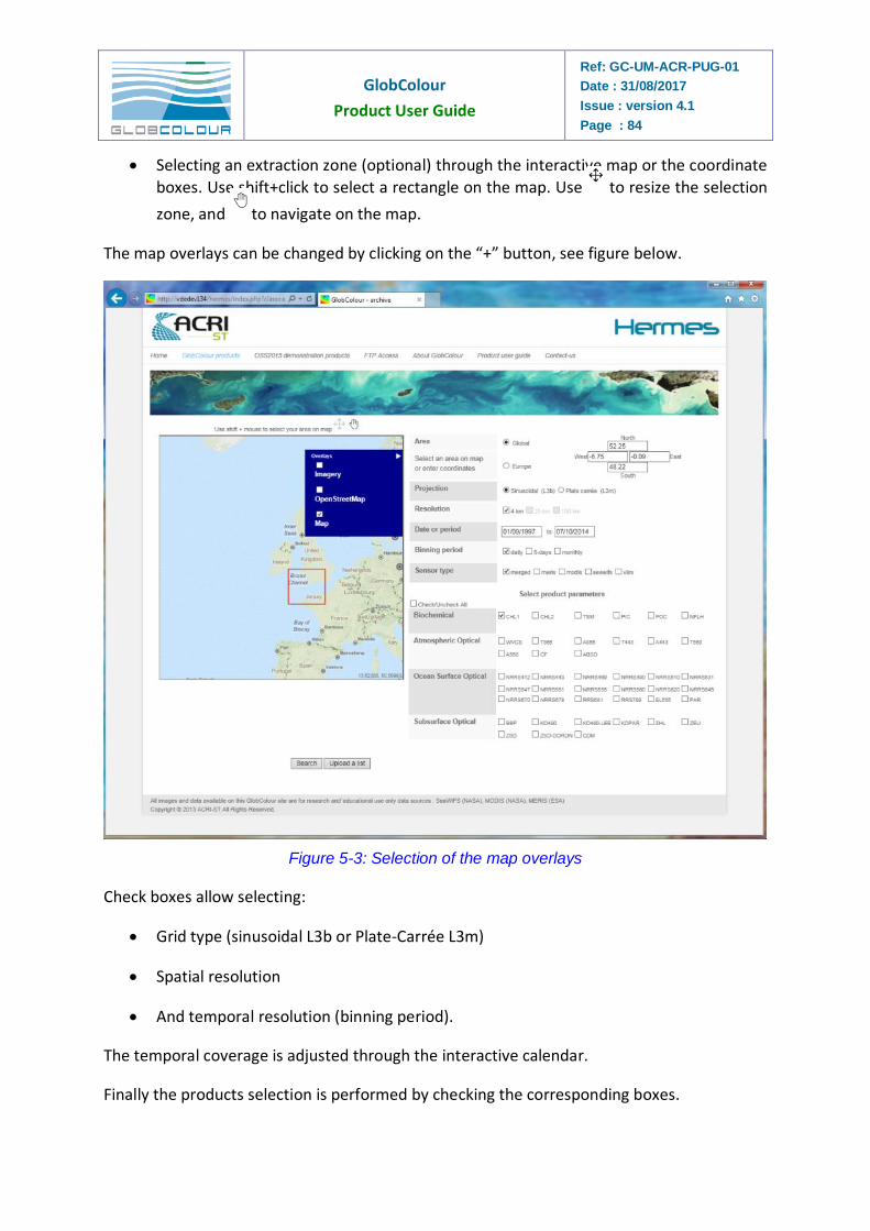
GlobColour

Product User Guide


Date : 31/08/2017

Issue : version 4.1

Page : 84

Selecting an extraction zone (optional) through the interactive map or the coordinate

boxes. Use shift+click to select a rectangle on the map. Use to resize the selection

zone, and to navigate on the map.

The map overlays can be changed by clicking on the “+” button, see figure below.

Figure 5-3: Selection of the map overlays

Check boxes allow selecting:

Grid type (sinusoidal L3b or Plate-Carrée L3m)

Spatial resolution

And temporal resolution (binning period).

The temporal coverage is adjusted through the interactive calendar.

Finally the products selection is performed by checking the corresponding boxes.

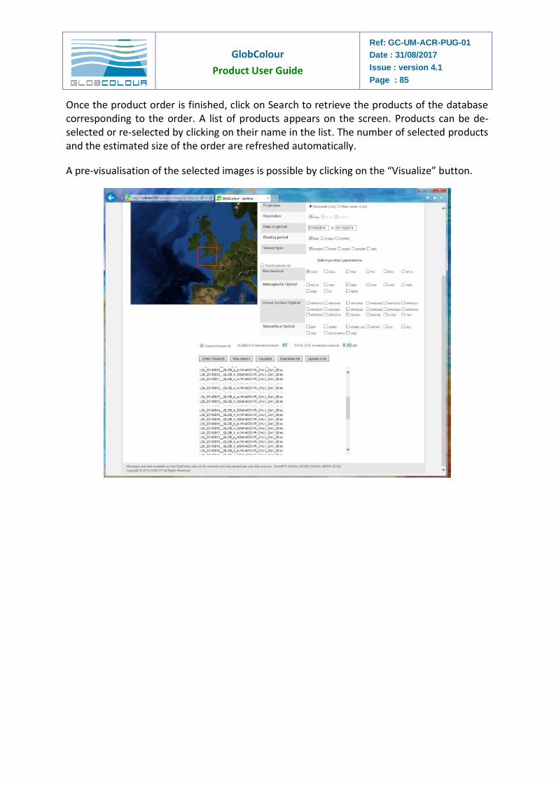
GlobColour

Product User Guide


Date : 31/08/2017

Issue : version 4.1

Page : 85

Once the product order is finished, click on Search to retrieve the products of the database corresponding to the order. A list of products appears on the screen. Products can be de-selected or re-selected by clicking on their name in the list. The number of selected products and the estimated size of the order are refreshed automatically.

A pre-visualisation of the selected images is possible by clicking on the “Visualize” button.

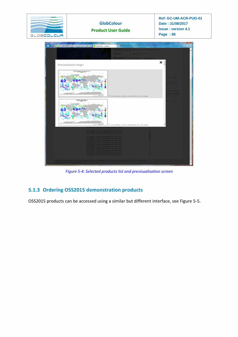
GlobColour

Product User Guide


Date : 31/08/2017

Issue : version 4.1

Page : 86

Figure 5-4: Selected products list and previsualisation screen

5.1.3 Ordering OSS2015 demonstration products

OSS2015 products can be accessed using a similar but different interface, see Figure 5-5.

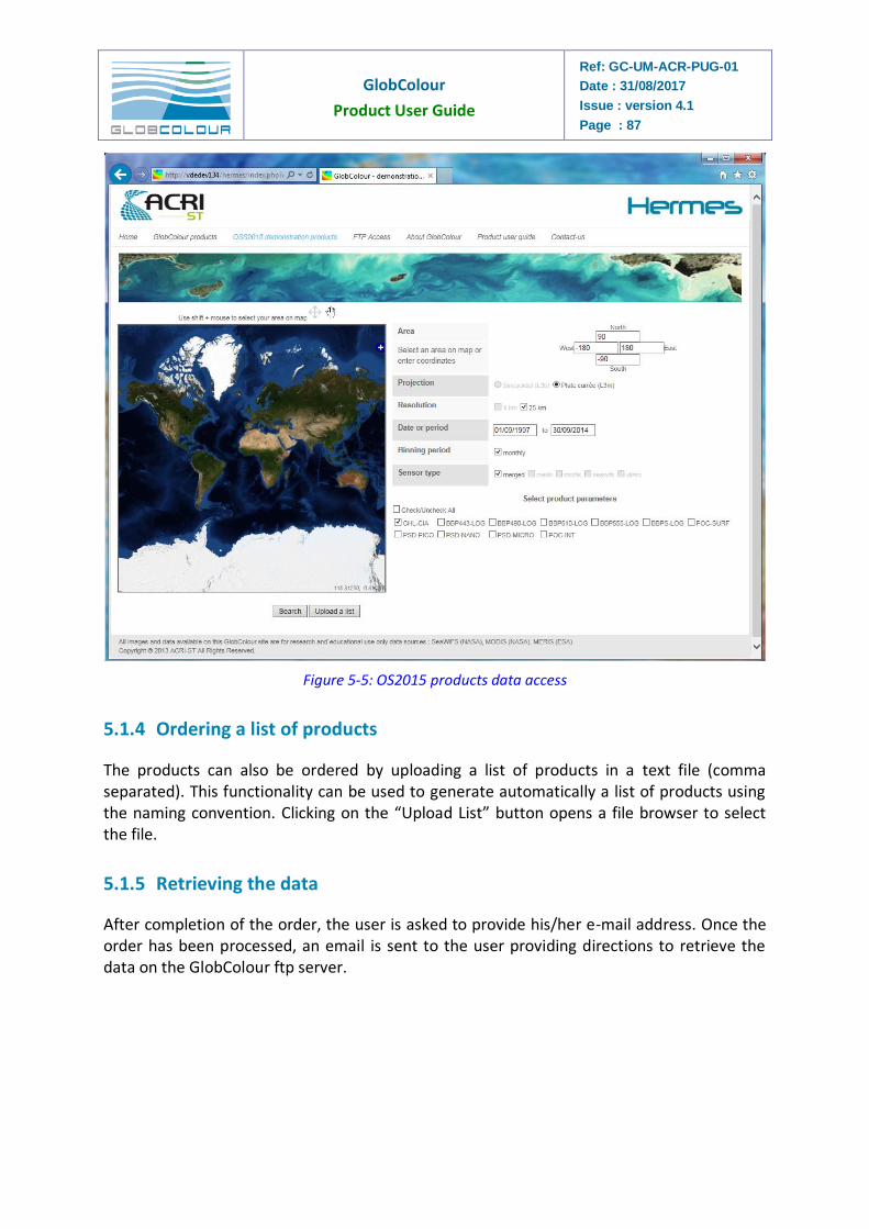
GlobColour

Product User Guide


Date : 31/08/2017

Issue : version 4.1

Page : 87

Figure 5-5: OS2015 products data access

5.1.4 Ordering a list of products

The products can also be ordered by uploading a list of products in a text file (comma separated). This functionality can be used to generate automatically a list of products using the naming convention. Clicking on the “Upload List” button opens a file browser to select the file.

5.1.5 Retrieving the data

After completion of the order, the user is asked to provide his/her e-mail address. Once the order has been processed, an email is sent to the user providing directions to retrieve the data on the GlobColour ftp server.

GlobColour

Product User Guide


Date : 31/08/2017

Issue : version 4.1

Page : 88

5.2 Download the data from the GlobColour ftp server

The GlobColour project maintains an ftp site from where the products can be downloaded. Read the information provided by the GlobColour web site ("Data Access" section) to get the latest news about this service.

The current ftp server is ftp://ftp.hermes.acri.fr

Login and passwords can be obtained by filling the request on-line on the hermes page “FTP access”.

The distribution structure of the ftp archive is:

/zone (GLOB|EURO) /sensor (seawifs|meris|modis|viirsn|olcia|merged) /binning period (day|8-day|month) /yyyy/mm/dd

Each directory contains the netCDF products (L3b*.nc|L3m*.nc) as well as the associated “quicklook” images.

The ftp also delivers the third party products (NPP and PFT).

A convenient way to download the products is to use the Unix wget command. This command is also available in the cygwin package for Windows systems. wget is particularly efficient to download specific files from scattered sub-directories. It can be used also to check for new products - mirroring (already downloaded files are not transferred, updated products on the server are transferred).

Here is an example for downloading all the MERIS CDM binned products. You can adapt this command to your specific needs. The specification of the GlobColour products filenames is useful to use the correct wildcarding included in the wget commands.

wget -r -l10 -t10 -A "L3b*_4_*MER_CDM*.nc" -w3 -Q1000m \

ftp://GlobColour_data:[email protected]/GLOB/meris/ ./

Another example to download all the CHL1 monthly quicklooks at 25 km resolution.

wget -r -l10 -t10 -A "L3m*_25_*CHL1_MO*.nc" -w3 -Q1000m \

ftp://GlobColour_data:[email protected]/GLOB/merged ./

The products will be stored in a local directory called ftp.fr-acri.com using the same structure as on the ftp server. All options of the wget command are described at:

http://www.gnu.org/software/wget/manual/wget.html

The following options are recommended:

-w3 is specified to pause the process 3s after each download to decrease our server load by

making the requests less frequent. Please keep it to share the bandwidth with other users.

-Q1000m limits the amount of data you can retrieve in one command (1 Gb). Please, keep

this option too.

5.3 Read the data

The products may be read using the netCDF library or any third-party tool reading netCDF files. The format of the data is provided in a dedicated chapter ("The Products format").

ftp://ftp.hermes.acri.fr/

http://www.gnu.org/software/wget/manual/wget.html

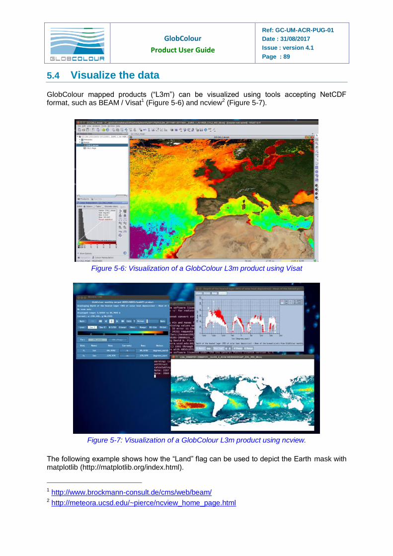
GlobColour

Product User Guide


Date : 31/08/2017

Issue : version 4.1

Page : 89

5.4 Visualize the data

GlobColour mapped products (“L3m”) can be visualized using tools accepting NetCDF format, such as BEAM / Visat1 (Figure 5-6) and ncview2 (Figure 5-7).

Figure 5-6: Visualization of a GlobColour L3m product using Visat

Figure 5-7: Visualization of a GlobColour L3m product using ncview.

The following example shows how the “Land” flag can be used to depict the Earth mask with matplotlib (http://matplotlib.org/index.html).

1 http://www.brockmann-consult.de/cms/web/beam/ 2 http://meteora.ucsd.edu/~pierce/ncview_home_page.html

http://www.brockmann-consult.de/cms/web/beam/

http://meteora.ucsd.edu/~pierce/ncview_home_page.html

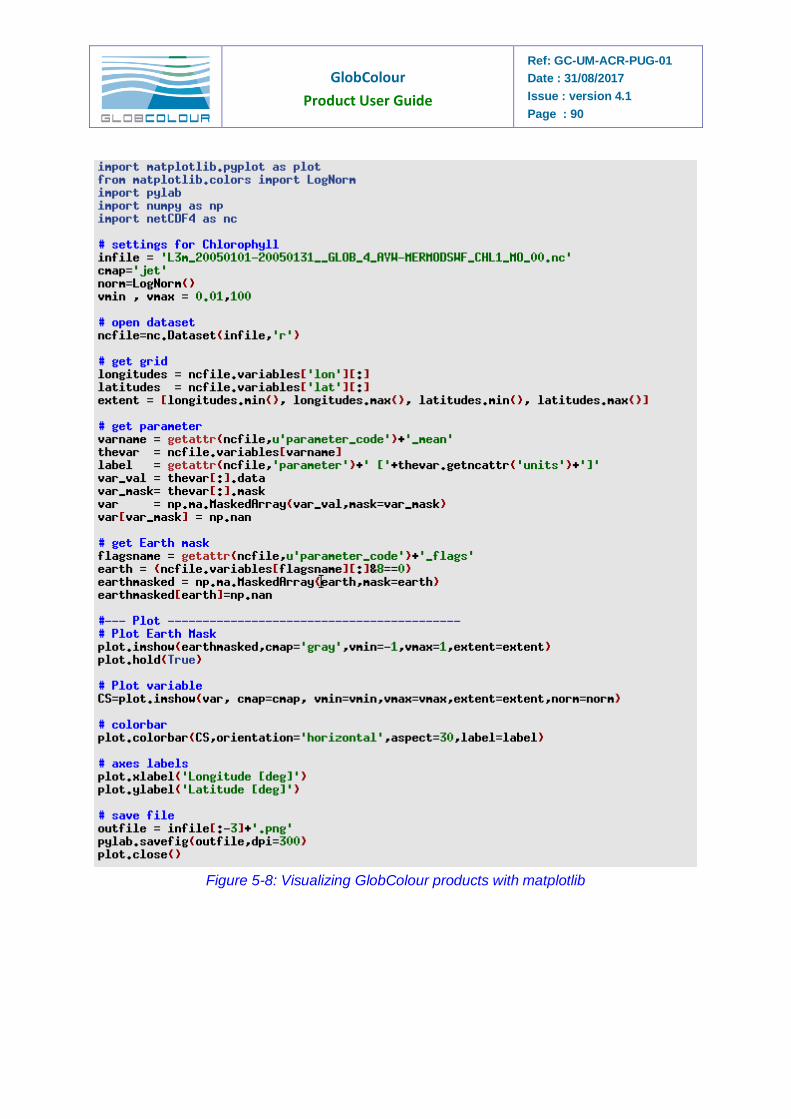
GlobColour

Product User Guide


Date : 31/08/2017

Issue : version 4.1

Page : 90

Figure 5-8: Visualizing GlobColour products with matplotlib

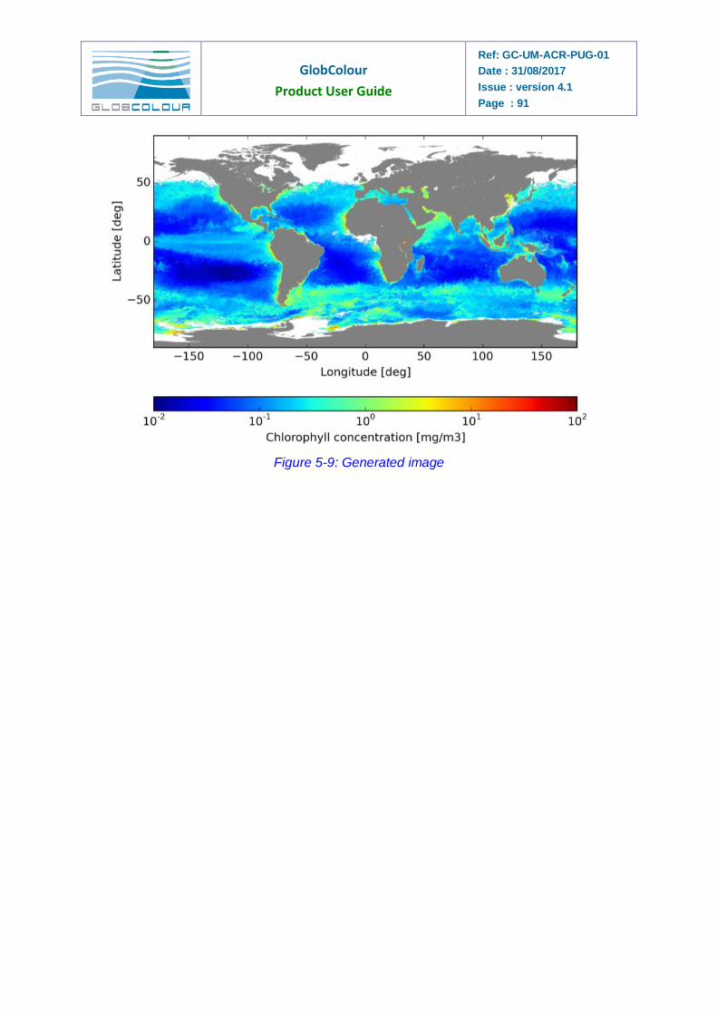
GlobColour

Product User Guide


Date : 31/08/2017

Issue : version 4.1

Page : 91

Figure 5-9: Generated image

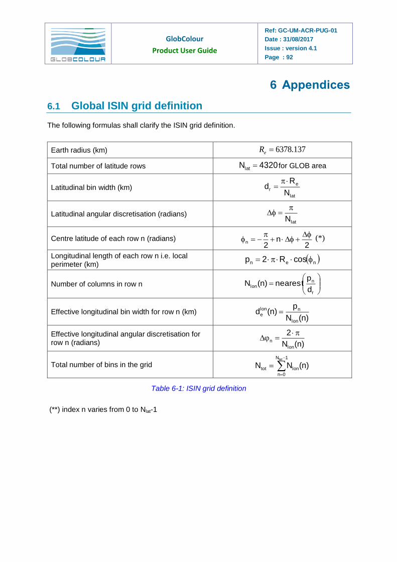
GlobColour

Product User Guide


Date : 31/08/2017

Issue : version 4.1

Page : 92

6 Appendices

6.1 Global ISIN grid definition

The following formulas shall clarify the ISIN grid definition.

Earth radius (km) 137.6378eR

Total number of latitude rows 4320Nlat for GLOB area

Latitudinal bin width (km) lat

er

N

Rd

Latitudinal angular discretisation (radians) latN

Centre latitude of each row n (radians) 2

n2

n

(*)

Longitudinal length of each row n i.e. local perimeter (km)

nen cosR2p

Number of columns in row n

r

nlon

d

pnearest)n(N

Effective longitudinal bin width for row n (km) )n(N

p)n(d

lon

nlon

e

Effective longitudinal angular discretisation for row n (radians) )n(N

2

lon

n

Total number of bins in the grid

1N

0n

lontot

lat

)n(NN

Table 6-1: ISIN grid definition

(**) index n varies from 0 to Nlat-1

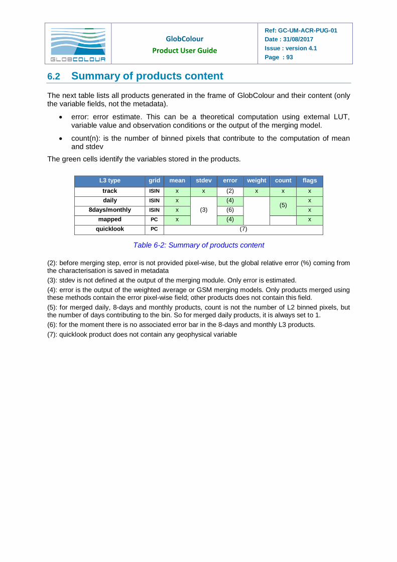
GlobColour

Product User Guide


Date : 31/08/2017

Issue : version 4.1

Page : 93

6.2 Summary of products content

The next table lists all products generated in the frame of GlobColour and their content (only the variable fields, not the metadata).

error: error estimate. This can be a theoretical computation using external LUT, variable value and observation conditions or the output of the merging model.

count(n): is the number of binned pixels that contribute to the computation of mean and stdev

The green cells identify the variables stored in the products.

L3 type grid mean stdev error weight count flags

track ISIN x x (2) x x x

daily ISIN x

(3)

(4)

(5)

x

8days/monthly ISIN x (6) x

mapped PC x (4) x

quicklook PC (7)

Table 6-2: Summary of products content

(2): before merging step, error is not provided pixel-wise, but the global relative error (%) coming from the characterisation is saved in metadata

(3): stdev is not defined at the output of the merging module. Only error is estimated.

(4): error is the output of the weighted average or GSM merging models. Only products merged using these methods contain the error pixel-wise field; other products does not contain this field.

(5): for merged daily, 8-days and monthly products, count is not the number of L2 binned pixels, but the number of days contributing to the bin. So for merged daily products, it is always set to 1.

(6): for the moment there is no associated error bar in the 8-days and monthly L3 products.

(7): quicklook product does not contain any geophysical variable

GlobColour

Product User Guide


Date : 31/08/2017

Issue : version 4.1

Page : 94

6.3 The main characteristics of the products

The following lists summarises the main characteristics of the different products generated in the frame of the GlobColour project. Note that not all these products are available to external users (internal products are written in dark blue).

Level 3 track global at 4.63 km (ISIN grid):

global product

one variable per file

no observation geometry

only valid bins are written in the product

Level 3 daily global at 4.63 km (ISIN grid):

computed from the level 3 track global products

same as for the level 3 track global at 4.63 km (ISIN grid), single instrument product, except:

temporal binning algorithm using GlobColour data-day definition

weight is the sum of weight at track level

Level 3 merged global at 4.63 km (ISIN grid):

computed from the level 3 daily global products using one merging method

multi-instruments product

same format as for the level 3 daily global products, except:

no weight and stdev fields

the "mean" field is an output of the merging model

only the weighted average and GSM model merging method provides the pixel-wise error (stored in the “error” field)

parameters with no characterised error are not merged using the weighted average method

the global relative error (%) is stored in the variable attribute pct_characterised_error. It is actually set to the maximum of the global relative characterised errors for each input sensor.

for merged daily, 8-days and monthly products, count is not the number of L2 binned pixels, but the number of days contributing to the bin. At this step it is always set to 1.

Level 3 8-days/monthly global at 4.63 km (ISIN grid):

computed from the level 3 merged daily products

temporal binning algorithm applied

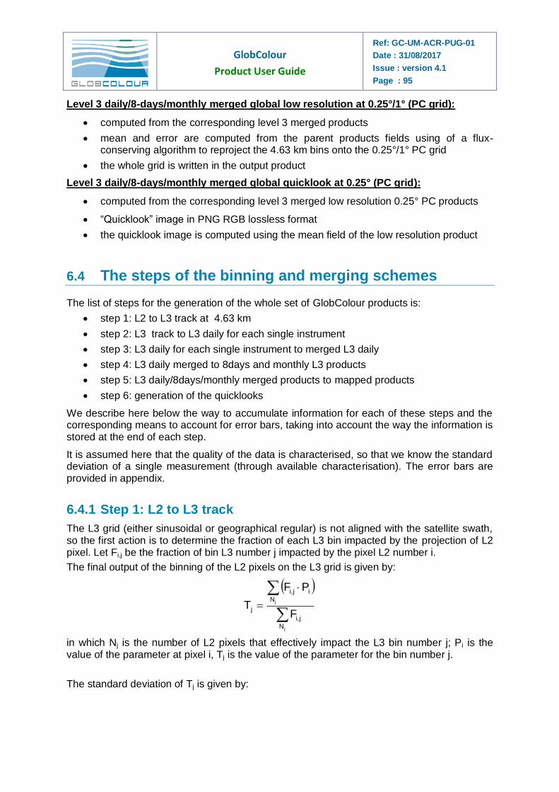
GlobColour

Product User Guide


Date : 31/08/2017

Issue : version 4.1

Page : 95

Level 3 daily/8-days/monthly merged global low resolution at 0.25°/1° (PC grid):

computed from the corresponding level 3 merged products

mean and error are computed from the parent products fields using of a flux-conserving algorithm to reproject the 4.63 km bins onto the 0.25°/1° PC grid

the whole grid is written in the output product

Level 3 daily/8-days/monthly merged global quicklook at 0.25° (PC grid):

computed from the corresponding level 3 merged low resolution 0.25° PC products

“Quicklook” image in PNG RGB lossless format

the quicklook image is computed using the mean field of the low resolution product

6.4 The steps of the binning and merging schemes

The list of steps for the generation of the whole set of GlobColour products is:

step 1: L2 to L3 track at 4.63 km

step 2: L3 track to L3 daily for each single instrument

step 3: L3 daily for each single instrument to merged L3 daily

step 4: L3 daily merged to 8days and monthly L3 products

step 5: L3 daily/8days/monthly merged products to mapped products

step 6: generation of the quicklooks

We describe here below the way to accumulate information for each of these steps and the corresponding means to account for error bars, taking into account the way the information is stored at the end of each step.

It is assumed here that the quality of the data is characterised, so that we know the standard deviation of a single measurement (through available characterisation). The error bars are provided in appendix.

6.4.1 Step 1: L2 to L3 track

The L3 grid (either sinusoidal or geographical regular) is not aligned with the satellite swath, so the first action is to determine the fraction of each L3 bin impacted by the projection of L2 pixel. Let Fi,j be the fraction of bin L3 number j impacted by the pixel L2 number i.

The final output of the binning of the L2 pixels on the L3 grid is given by:

j

j

N

j,i

N

ij,i

jF

PF

T

in which Nj is the number of L2 pixels that effectively impact the L3 bin number j; Pi is the value of the parameter at pixel i, Tj is the value of the parameter for the bin number j.

The standard deviation of Tj is given by:

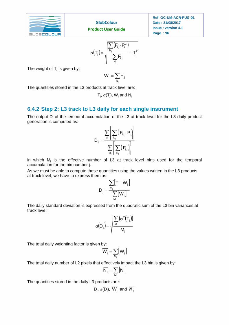
GlobColour

Product User Guide


Date : 31/08/2017

Issue : version 4.1

Page : 96

2

j

N

j,i

N

2

ij,i

j TF

PF

T

j

j

The weight of Tj is given by:

jN

j,ij FW

The quantities stored in the L3 products at track level are:

Tj, (Tj), Wj and Nj

6.4.2 Step 2: L3 track to L3 daily for each single instrument

The output Dj of the temporal accumulation of the L3 at track level for the L3 daily product generation is computed as:

j j

j j

M N

j,i

M N

ij,i

j

F

PF

D

in which Mj is the effective number of L3 at track level bins used for the temporal accumulation for the bin number j.

As we must be able to compute these quantities using the values written in the L3 products at track level, we have to express them as:

j

j

M

j

M

j

jW

WT

D

The daily standard deviation is expressed from the quadratic sum of the L3 bin variances at track level:

j

M

j

2

jM

T

D j

The total daily weighting factor is given by:

jM

jj WW

The total daily number of L2 pixels that effectively impact the L3 bin is given by:

jM

jj NN

The quantities stored in the daily L3 products are:

Dj, (Dj), jW and jN

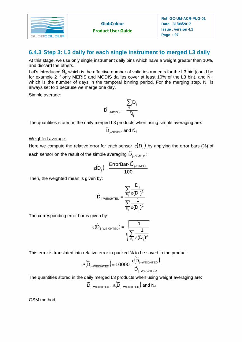
GlobColour

Product User Guide


Date : 31/08/2017

Issue : version 4.1

Page : 97

6.4.3 Step 3: L3 daily for each single instrument to merged L3 daily

At this stage, we use only single instrument daily bins which have a weight greater than 10%, and discard the others.

Let’s introduced Ñj, which is the effective number of valid instruments for the L3 bin (could be for example 2 if only MERIS and MODIS dailies cover at least 10% of the L3 bin), and Ñd, which is the number of days in the temporal binning period. For the merging step, Ñd is always set to 1 because we merge one day.

Simple average:

j

Ñ

j

SIMPLEjÑ

D

D~ j

The quantities stored in the daily merged L3 products when using simple averaging are:

SIMPLEjD~

and Ñd

Weighted average:

Here we compute the relative error for each sensor jD by applying the error bars (%) of

each sensor on the result of the simple averaging SIMPLEjD

~

:

100

D~

ErrorBarD

SIMPLEj

j

Then, the weighted mean is given by:

j

j

Ñ2

j

Ñ2

j

j

WEIGHTEDj

)D(

1

)D(

D

D~

The corresponding error bar is given by:

jÑ2

j

WEIGHTEDj

)D(

1

1)D

~(

This error is translated into relative error in packed % to be saved in the product:

WEIGHTEDj

WEIGHTEDj

WEIGHTEDjD~D~

10000D~

The quantities stored in the daily merged L3 products when using weight averaging are:

WEIGHTEDjD~

, WEIGHTEDjD

~ and Ñd

GSM method

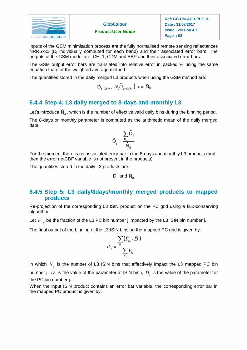
GlobColour

Product User Guide


Date : 31/08/2017

Issue : version 4.1

Page : 98

Inputs of the GSM minimisation process are the fully normalised remote sensing reflectances NRRSxxx (Dj individually computed for each band) and their associated error bars. The outputs of the GSM model are: CHL1, CDM and BBP and their associated error bars.

The GSM output error bars are translated into relative error in packed % using the same equation than for the weighted average method.

The quantities stored in the daily merged L3 products when using the GSM method are:

GSMjD~

, GSMjD

~ and Ñd

6.4.4 Step 4: L3 daily merged to 8-days and monthly L3

Let’s introduce dN̂ , which is the number of effective valid daily bins during the binning period.

The 8-days or monthly parameter is computed as the arithmetic mean of the daily merged data.

d

N̂

j

jN̂

D~

D̂ d

For the moment there is no associated error bar in the 8-days and monthly L3 products (and then the error netCDF variable is not present in the products).


jD̂ and dN̂

6.4.5 Step 5: L3 daily/8days/monthly merged products to mapped products

Re-projection of the corresponding L3 ISIN product on the PC grid using a flux-conserving algorithm:

Let jiF ,

be the fraction of the L3 PC bin number j impacted by the L3 ISIN bin number i.

The final output of the binning of the L3 ISIN bins on the mapped PC grid is given by:

j

j

N

ji

N

iji

jF

DF

D

,

,

in which jN

is the number of L3 ISIN bins that effectively impact the L3 mapped PC bin

number j; iD is the value of the parameter at ISIN bin i, jD

is the value of the parameter for

the PC bin number j.

When the input ISIN product contains an error bar variable, the corresponding error bar in the mapped PC product is given by:

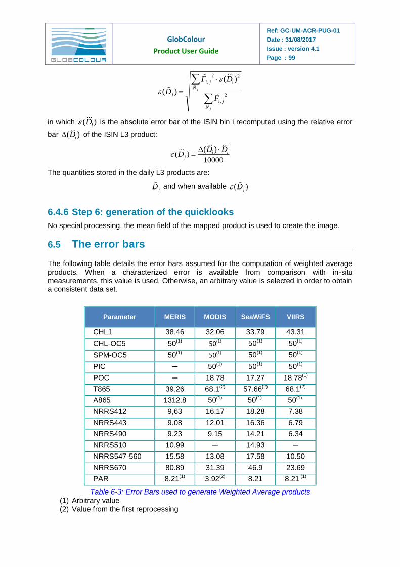
GlobColour

Product User Guide


Date : 31/08/2017

Issue : version 4.1

Page : 99

j

j

N

ji

N

iji

jF

DF

D

2

,

22

, )(

)(

in which )( iD is the absolute error bar of the ISIN bin i recomputed using the relative error

bar )( iD of the ISIN L3 product:

10000

)()( ii

j

DDD


jD

and when available )( jD

6.4.6 Step 6: generation of the quicklooks

No special processing, the mean field of the mapped product is used to create the image.

6.5 The error bars

The following table details the error bars assumed for the computation of weighted average products. When a characterized error is available from comparison with in-situ measurements, this value is used. Otherwise, an arbitrary value is selected in order to obtain a consistent data set.

Parameter MERIS MODIS SeaWiFS VIIRS

CHL1 38.46 32.06 33.79 43.31

CHL-OC5 50(1) 50(1) 50(1) 50(1)

SPM-OC5 50(1) 50(1) 50(1) 50(1)

PIC ─ 50(1) 50(1) 50(1)

POC ─ 18.78 17.27 18.78(1)

T865 39.26 68.1(2) 57.66(2) 68.1(2)

A865 1312.8 50(1) 50(1) 50(1)

NRRS412 9,63 16.17 18.28 7.38

NRRS443 9.08 12.01 16.36 6.79

NRRS490 9.23 9.15 14.21 6.34

NRRS510 10.99 ─ 14.93 ─

NRRS547-560 15.58 13.08 17.58 10.50

NRRS670 80.89 31.39 46.9 23.69

PAR 8.21(1) 3.92(2) 8.21 8.21 (1)

Table 6-3: Error Bars used to generate Weighted Average products (1) Arbitrary value (2) Value from the first reprocessing

GlobColour

Product User Guide


Date : 31/08/2017

Issue : version 4.1

Page : 100

6.6 Common Data Language description

CDL representation of a global mapped level-3 daily merged product: netcdf L3m_20120301-20120331__GLOB_4_AVW-MERMODVIR_CHL1_MO_00 {

dimensions:

lat = 4320 ;

lon = 8640 ;

variables:

float lat(lat) ;

lat:long_name = "latitude" ;

lat:units = "degrees_north" ;

lat:axis = "Y" ;

float lon(lon) ;

lon:long_name = "longitude" ;

lon:units = "degrees_east" ;

lon:axis = "X" ;

float CHL1_mean(lat, lon) ;

CHL1_mean:standard_name = "mass_concentration_of_chlorophyll_a_in_sea_water" ;

CHL1_mean:long_name = "Chlorophyll concentration - Mean of the binned pixels" ;

CHL1_mean:_FillValue = -999.f ;

CHL1_mean:units = "mg/m3" ;

CHL1_mean:pct_characterised_error = 43.31f ;

short CHL1_flags(lat, lon) ;

CHL1_flags:long_name = "Chlorophyll concentration - Flags" ;

CHL1_flags:_FillValue = 0s ;

short CHL1_error(lat, lon) ;

CHL1_error:long_name = "Chlorophyll concentration - Error estimation" ;

CHL1_error:_FillValue = -32768s ;

CHL1_error:units = "%" ;

CHL1_error:scale_factor = 0.01f ;

// global attributes:

:Conventions = "CF-1.4" ;

:title = "GlobColour monthly merged MERIS/MODIS/VIIRSN product" ;

:product_name = "L3m_20120301-20120331__GLOB_4_AVW-MERMODVIR_CHL1_MO_00.nc" ;

:product_type = "month" ;

:product_level = 3s ;

GlobColour

Product User Guide


Date : 31/08/2017

Issue : version 4.1

Page : 101

:parameter_code = "CHL1" ;

:parameter = "Chlorophyll concentration" ;

:parameter_algo_list = "OC4Me,OC3v5,OC3v5" ;

:site_name = "GLOB" ;

:sensor_name = "WEIGHTED_AVERAGING" ;

:sensor = "Merged data - weighted mean" ;

:sensor_name_list = "MER,MOD,VIR" ;

:start_time = "20120229T214722Z" ;

:end_time = "20120401T025400Z" ;

:duration_time = "PT2696799S" ;

:period_start_day = "20120301" ;

:period_end_day = "20120331" ;

:period_duration_day = "P31D" ;

:grid_type = "Equirectangular" ;

:spatial_resolution = 4.638312f ;

:nb_equ_bins = 8640 ;

:registration = 5 ;

:lat_step = 0.04166667f ;

:lon_step = 0.04166667f ;

:earth_radius = 6378.137 ;

:max_north_grid = 90.f ;

:max_south_grid = -90.f ;

:max_west_grid = -180.f ;

:max_east_grid = 180.f ;

:northernmost_latitude = 74.41666f ;

:southernmost_latitude = -76.25001f ;

:westernmost_longitude = -180.f ;

:easternmost_longitude = 180.f ;

:nb_grid_bins = 37324800 ;

:nb_bins = 37324800 ;

:pct_bins = 100.f ;

:nb_valid_bins = 19406411 ;

:pct_valid_bins = 51.99334f ;

:software_name = "globcolour_l3_reproject" ;

:institution = "ACRI" ;

:processing_time = "20140724T080509Z" ;

:netcdf_version = "4.1.3 of Sep 5 2011 16:53:33 $" ;

:DPM_reference = "GC-UD-ACRI-PUG" ;

:IODD_reference = "GC-UD-ACRI-PUG" ;

:references = "http://www.globcolour.info" ;

:contact = "[email protected]" ;

http://www.globcolour.info/

mailto:[email protected]

GlobColour

Product User Guide


Date : 31/08/2017

Issue : version 4.1

Page : 102

:history = "20140724T080509Z: globcolour_l3_reproject.sh -inlist globcolour/data/merged/month/2012/03/01 -outdir globcolour/data/merged/month/2012/03/01 -startdataday 20120301 -enddataday 20120331 -resolution 0.041666666666666664 -resolutioncode 4 -tmpdir /work/scratch" ;

:input_files = "…"

:input_files_reprocessings = "…"

:product_version = "2014.0" ;

:software_version = "2014.0" ;

:copyright = "Copyright ACRI-ST - GlobColour. GlobColour has been originally funded by ESA with data from ESA, NASA, NOAA and GeoEye. This reprocessing version has received funding from the European Community’s Seventh Framework Programme ([FP7/2007-2013]) under grant agreement n° 282723 [OSS2015 project]." ;

}

GlobColour

Product User Guide


Date : 31/08/2017

Issue : version 4.1

Page : 103

6.7 References

6.7.1 GlobColour products references

Antoine, D., André J.M. and A. Morel (1996). Oceanic primary production: II. Estimation at global scale from satellite (Coastal Zone Color Scanner) chlorophyll, Global Biogeochemical Cycles, 10, 57-69.

Bailey, S.W., McClain, C.R., Werdell, P.J. and Schieber, B.D. (2000) Chapter 7: Normalised Water-Leaving Radiance and Chlorophyll a Match-Up Analyses. NASA Tech. Memo. 206892, Vol. 10, S.B. Hooker, and E.R. Firestone, Eds., NASA Goddard Space Flight Center, Greenbelt, Maryland, pp 45-52.

Doron, M., Babin, M., Mangin, A. and O. Fanton d'Andon (2006). Estimation of light penetration, and horizontal and vertical visibility in oceanic and coastal waters from surface reflectance. Journal of Geophysical Research, volume 112, C06003, doi: 10.1029/2006JC004007.

Feldman, G.C. (2005b) MODIS/Aqua Ocean Reprocessing 1.1 http://oceancolor.gsfc.nasa.gov/REPROCESSING/Aqua/R1.1/. Accessed December 2005.

Feldman, G.C. (2005c) SeaWiFS Ocean Reprocessing 5.1: http://oceancolor.gsfc.nasa.gov/REPROCESSING/SeaWiFS/R5.1/. Accessed December 2005.

Feldman, G.C. (2005d) MSl12: The Multi-Sensor Level-1 to Level-2 Code http://oceancolor.gsfc.nasa.gov/DOCS/MSL12/. Accessed January 2006.

Feldman, G.C. (2006) Oceancolor Products. http://oceancolor.gsfc.nasa.gov/PRODUCTS/. Access January 2006.

IOCCG (1998) Minimum Requirements for an Operational, Ocean-Colour Sensor for the Open Ocean, IOCCG Report Number 1, 50 pp.

IOCCG (1999). Status and Plans for Satellite Ocean-Colour Missions: Considerations for Complementary Missions. Yoder, J. A. (ed.), Reports of the International Ocean-Colour Coordinating Group, No. 2, IOCCG, Dartmouth, Canada. ISSN: 1098-6030

IOCCG Report No. 4, Guide to the creation and use of ocean-colour, Level-3, binned data products, D. Antoine (ed.), 2004. http://www.ioccg.org/reports_ioccg.html

IOCCG (2006). Ocean Colour Data Merging. Gregg, W.W. (ed.), Reports of the International Ocean-Colour Coordinating Group, No. 5, IOCCG.


http://oceancolor.gsfc.nasa.gov/REPROCESSING/Aqua/R1.1/

http://oceancolor.gsfc.nasa.gov/REPROCESSING/SeaWiFS/R5.1/

http://oceancolor.gsfc.nasa.gov/DOCS/MSL12/

http://oceancolor.gsfc.nasa.gov/PRODUCTS/

GlobColour

Product User Guide


Date : 31/08/2017

Issue : version 4.1

Page : 104

Maritorena S., Siegel, D.A. and Peterson, A. (2002) Optimization of a Semi-Analytical Ocean Colour Model for Global Scale Applications. Applied Optics, 41, 15, 2705-2714.

MODIS (2005) http://oceancolor.gsfc.nasa.gov/DOCS/MODISA_processing.html. Accessed December 2005.

André Morel, Yannick Huot, Bernard Gentili, P. Jeremy Werdell, Stanford B. Hooker, Bryan A. Franz, “Examining the consistency of products derived from various ocean color sensors in open ocean (Case 1) waters in the perspective of a multi-sensor approach”, Remote Sensing of Environment, 111 (2007), 69-88, doi:10.1016/j.rse.2007.03.012

Morel, A. and S. Bélanger, (2006) Improved Detection of turbid waters from Ocean Color information, Remote Sensing of Environment, 102, 237-249

Morel, A. and Antoine, D. (2000) Pigment Index Retrieval in Case 1 Waters, MERIS ATBD 2.9, Issue 4, Revision 2, 26 pp.

Morel, A., Antoine, D. and Gentilli, B. (2002) Bidirectional reflectance of oceanic waters: accounting for Raman emission and varying particle scattering phase function, Applied Optics, 41, 6289-6306

Morel, A., Huot, Y., Gentili, B., Werdell, P.J., Hooker, S.B. and B.A. Franz (2007). Examining the consistency of products derived from various ocean color sensors in open ocean (Case 1) waters in the perspective of a multi-sensor approach. Remote Sensing of Environment, 111, 69-88.

Orbimage Inc. (2005) http://www.orbimage.com/prods/orbview_2_prodinfo.htm. Accessed December

2005.

Frouin, R., B. A. Franz, and P. J. Werdell, 2003: The SeaWiFS PAR product. In Algorithm Updates for the Fourth SeaWiFS Data Reprocessing, S. B. Hooker and E. R. Firestone, Editors, CC NASA/TM-2003-206892, Vol. 22, 46-50.

Morel, A. and Gentili, B.: A simple band ratio technique to quantify the colored dissolved and detrital organic material from ocean color remotely sensed data, Remote Sens. Environ., 113, 998–1011, 2009a.

Zhong-Ping Lee, Ke-Ping Du and Robert Arnone (2005) A model for the diffuse attenuation

coefficient of downwelling irradiance. JOURNAL OF GEOPHYSICAL RESEARCH. VOL. 110, C02016, doi:10.1029/2004JC002275, 2005.

Saulquin, B., Hamdi, A., Gohin, F., Populus, J., Mangin, A., & d'Andon, O. F. (2013). Estimation of the diffuse attenuation coefficient KdPAR using MERIS and application to seabed habitat mapping. Remote Sensing of Environment, 128, 224-233.

http://oceancolor.gsfc.nasa.gov/DOCS/MODISA_processing.html

http://dx.doi.org/10.1016/j.rse.2007.03.012

http://www.orbimage.com/prods/orbview_2_prodinfo.htm.%20Accessed%20December%202005

http://www.orbimage.com/prods/orbview_2_prodinfo.htm.%20Accessed%20December%202005

http://faculty.umb.edu/zhongping.lee/Files/Lee_2005_Kd1.pdf

http://faculty.umb.edu/zhongping.lee/Files/Lee_2005_Kd1.pdf

GlobColour

Product User Guide


Date : 31/08/2017

Issue : version 4.1

Page : 105


6.7.2 References for OSS2015 demonstration products

Antoine, D. and A. Morel (1996). Oceanic primary production : I. Adaptation of a spectral light-photosynthesis model in view of application to satellite chlorophyll observations, Global Biogeochemical Cycles, 10, 43-55.

Claustre, H., Sciandra A., and D. Vaulot (2008), Introduction to the special section Bio-optical and biogeochemical conditions in the South East Pacific in late 2004: the BIOSOPE program. Biogeosciences, 5, 679-691.

Claustre H., Morel A., Babin M., Cailliau C., Marie D., Marty J. C., Talliez D., Vaulot D., 1999. “Variability in particle attenuation and chlorophyll fluorescence in the tropical Pacific: Scales, patterns and biogeochemical implications”. Journal of Geophysical Research, 104, pp. 3401-3422.

Campbell, J.W., Blaisdell, J.M., and Darzi, M., (1995).SeaWIFS Technical Report Series, NASA Vol. 32, Level-3 SeaWIFS Data Products: Spatial and Temporal Binning Algorithms. Edited by Hooker, S.B., Firestone, E.R., and Acker, J.G.

Carton, J. A. and B. S. Giese, 2008: A Reanalysis of Ocean Climate Using Simple Ocean Data Assimilation (SODA), Mon. Weather Rev., 136, 2999-3017.

de Boyer Montégut C., Madec G., Fischer A., LazarA., Ludicone D., 2004.”Mixed layer depth over the global ocean: an examination of profile data and profile-based climatology”. Journal of Geophysical Research, 108(C7),C12003,doi:10.1029/ 2004JC002378.

Duforêt-Gaurier L., Loisel H., Dessailly D., Nordkvist K., Alvain S., 2010. “ Estimates of particulate organic carbon over the euphotic depth from in situ measurements”. Application tosatellite data ove r the global ocean”. Deep-Sea Research, I 57 (2010) 351–367.

Eppley, R. W., Temperature and phytoplankton growth in the sea, Fish. Bull., 70, 1063-1084, 1972.

Garver, S.A., and Siegel, D., 1997. “ Inherent optical property inversion of ocean color spectra and its biogeochemical interpretation 1. Time series from the Sargossa Sea”. J. Geophys. Res. 102: 18607-18625.

Gordon, H. R., Brown, O. B., Evans, R. H., Brown, J. W., Smith, R. C., Baker, K. S. and Clark, D. K., 1988. “ A semianalytic radiance model of ocean color”? J. of Geoph. Res. 93(D9), 10909-10924.

Hu, C., Lee, Z., and Franz, B., 2012. “ Chlorophyll a algorithms for oligotrophic oceans: A novel approach bases on three-band reflectance difference”. Journal of Geophysical Research, 117, doi:10.1029/2011JC007395.

http://www.ocean-sci.net/7/705/2011/os-7-705-2011.pdf

http://www.ocean-sci.net/7/705/2011/os-7-705-2011.pdf

GlobColour

Product User Guide


Date : 31/08/2017

Issue : version 4.1

Page : 106

IOCCG, 2006. Remote sensing of inherent optical properties: fundamentals, tests of algorithms, and applications. In: Lee, Z. P. (Ed.), Reports of the International Ocean Color Coordinating Group, Vol. 5, IOCCG, Darthmouth, Canada, pp. 145.

Knap A., Michaels A., Close A., Ducklow H., Dickson A., 1996. “Protocols for the Joint Global Ocean Flux Study (JGOFS) Core Measurements”. JGOFS Report Nr. 19 (Reprint of the IOC Manuals and Guides no. 29, UNESCO, Paris, 1994), 170pp.

Kostadinov, T.S., D.A. Siegel, and S. Maritorena. 2009. Retrieval of the Particle Size Distribution from Satellite Ocean Color Observations. Journal of Geophysical Research, VOL. 114, C09015, doi:10.1029/2009JC005303.

Lee, Z., and K. L. Carder (2000), Band-ratio or spectral-curvature algorithms for satellite remote sensing, Appl. Opt.,39, 4377–4380, doi:10.1364/AO.39.004377.

H. Loisel and D. Stramski. 2000. Estimation of the inherent optical properties of natural waters from irradiance attenuation coefficient and reflectance in the presence of Raman scattering. Applied Optics. 39 : 3001-3011


Maritorena, S., Siegel, D. A., and Peterson, A. R., 2002. “ Optimization of a semi-analytical ocean color model for global-scale applications”. Applied Optics 41:2705-2714.

Maritorena S., Siegel, D.A. and Peterson, A. (2002) Optimization of a Semi-Analytical Ocean Colour Model for Global Scale Applications. Applied Optics, 41, 15, 2705-2714.

Morel, A., Antoine, D., Babin, M., and Y. Dandonneau (1996). Measured and modeled primary production in the Northeast Atlantic (EUMELI JGOFS program): The impact of natural variations in photosynthetic parameters on model predictive skill. Deep-Sea Research I, 43, 1273-1304.

Morel, A., and J.F. Berthon (1989). Surface pigments, algal biomass profiles, and potential production of the euphotic layer: Relationships reinvestigated in view of remote-sensing applications, Limnology and Oceanography, 34, 1545-1562.

Mobley, C. D. 1994. “Light and Water: Radiative Transfer in Natural Waters”. (Academic, San Diego, Calif., 1994

Monterey, G., Levitus, S., 1997. Seasonal Variability of Mixed Layer Depth for the World Ocean. NOAA Atlas NESDIS, vol. 14. U.S. Government Print Office, Washington, DC, 96pp.

Morel A., Maritorena S., 2001. “Bio-optical properties of oceanic waters: a reappraisal”. Journal of Geophysical Research. 106 (C4), 7163–7180.

Report of the International Ocean-Colour Coordinate Group, IOCCG Report Number 4, (2004).Edited by David Antoine.

Reynolds, R.W., N.A. Rayner, T.M. Smith, D.C. Stokes, and W. Wang, 2002: An improved in situ and satellite SST analysis for climate. J. Climate, 15, 1609-1625.

O’Reilly, J., S. Maritorena, B. G. Mitchell, D. Siegel, K. L. Carder, S. Garver, M. Kahru and C. McClain, 1998. “ Ocean color chlorophyll algorithms for SeaWiFS”, J. Geophys. Res. 103, 24, 937-24, 53.

GlobColour

Product User Guide


Date : 31/08/2017

Issue : version 4.1

Page : 107

O’Reilly, J. E. et al., 2000. “ SeaWiFS postlaunch calibration and validation analyses”, Part 3, NASA Tech. Memo., NASA, TM-2000-206892, vol. 11, 49 pp.

Stramska M., 2009. Particulate organic carbon in the global ocean derived from SeaWiFS ocean color. Deep-Sea Research. I 56 (9), 1459–1470.

Stramski D., Reynolds R.A., Babin M., Kaczmarek S., Lewis M.R., Rottgers R., Sciandra A., Stramska M., Twardowski M., Franz, B, Claustre, H., 2008. “Relationships between the surface concentration of particulate organic carbon and optical properties in the eastern South Pacific and eastern Atlantic Oceans”. Biogeosciences 5, 171–201.

Twardowski M, Boss E., Macdonald J., Pegau W., Barnard, A., Zaneveld, J., 2001. “A model for bulk refractive index from the optical backscattering ratio and the implications for understanding particle composition in case I and case II waters”. Journal of Geophysical Research. 106 (C7), 14129–14142.

Uitz J., Claustre H., Morel A., Hooker S.B., 2006. “Vertical distribution of phytoplankton communities in open ocean: an assessment based on surface chlorophyll”. Journal of Geophysical Research. 111, C08005, doi: 10.1029/2005JC003207.

Uitz, J., Claustre, H., Gentili, B. and D. Stramski (2010). Phytoplankton class-specific primary production in the world’s oceans: Seasonal and interannual variability from satellite observations. Global Biogeochemical Cycles, Vol. 24, No. 3, GB3016, doi: 10.1029/2009GB003680.

Uitz, J., Huot, Y., Bruyant, F., Babin, M. and H. Claustre (2008) Relating phytoplankton photophysiological properties to community structure on large scale, Limnology and Oceanography, 53(2), 614-630

Documents

GLOBCOLOUR · The GlobColour primary data set has now been delivered as a Group on Earth Observations ... LOV Laboratoire Océanologique de Villefranche-sur-mer