Embed Size (px)
Citation preview
𝑳𝟎 Stable Trigonometrically Fitted Block Backward Differentiation Formula of Adams Type for Autonomous
Oscillatory Problems
Solomon A. Okunuga* and R. I. Abdulganiy
Department of Mathematics, University of Lagos, Lagos, Nigeria. * Corresponding author. Tel.: +2348023244422; email: [email protected] Manuscript submitted April 6, 2016; accepted November 30, 2016. doi: 10.17706/ijapm.2017.7.2.128-133
Abstract: In this paper, a 𝐿0 Stable Second Derivative Trigonometrically Fitted Block Backward
Differentiation Formula of Adams Type (SDTFF) of algebraic order 4 is presented for the solution of
autonomous oscillatory problems. A Continuous Second Derivative Trigonometrically Fitted (CSDTF) whose
coefficients depend on the frequency and step size is constructed using trigonometric basis function. The
CSDTF is used to generate the main method and one additional method which are combined and applied in
block form as simultaneous numerical integrators. The stability properties of the method are investigated
using boundary locus plot. It is found that the method is zero stable, consistent and hence converges. The
method is applied on some numerical examples and the result show that the method is accurate and
efficient.
Key words: Autonomous oscillatory problems, backward differentiation formula, continuous scheme, trigonometrically fitted methods.
1. Introduction
An important and interesting class of initial value problems which arise in practice include the
differential equations whose solutions are known to oscillate with a fitting frequency. Such problems arise
frequently in area such as Biological Science, Economics, Chemical Kinetics, Theoretical Chemistry, Medical
Science to mention but a few.
The form and structure of the oscillating problems is highly application dependent [1]. They also noted
that the best numerical method to use is strongly dependent on the application. Numerical methods used to
treat oscillatory problems differ depending on the formulation of the problem, the knowledge of certain
characteristic of the solution and the objective of the computation [1].
A number of numerical methods based on the use of polynomial function have been developed for solving
this class of problems by various researchers such as [2]-[5]. Other methods based on exponential fitting
techniques which takes advantage of the special properties of the solution that may be known in advance
have also been proposed to solve this class of IVP (see [6], [7]).
In order to solve differential equations whose solutions are known to oscillate, methods based on
trigonometric polynomials have been proposed (see [8]-[13]). However, little attentions have been paid to
the Block Differentiation Formula using the trigonometric polynomial as the basis function for solving IVP
whose solution oscillate. Hence the motivation for this paper.
International Journal of Applied Physics and Mathematics
128 Volume 7, Number 2, April 2017
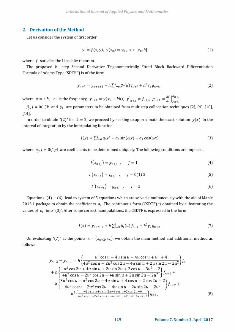
2. Derivation of the Method
Let us consider the system of first order
𝑦′= 𝑓 𝑥, 𝑦 , 𝑦 𝑥0 = 𝑦0 , 𝑥 ∈ 𝑥0, 𝑏 (1)
where 𝑓 satisfies the Lipschitz theorem
The proposed 𝑘 −step Second Derivative Trigonometrically Fitted Block Backward Differentiation
Formula of Adams Type (SDTFF) is of the form
𝑦𝑛+𝑘 = 𝑦𝑛+𝑘+1 + 𝛽𝑗 𝑢 𝑘𝑗 =0 𝑓𝑛+𝑗 + 2𝛾𝑘𝑔𝑛+𝑘 (2)
where 𝑢 = 𝜔, 𝜔 is the frequency, 𝑦𝑛+𝑘 = 𝑦 𝑥𝑛 + 𝑘 , 𝑦′𝑛+𝑘
= 𝑓𝑛+𝑗 , 𝑔𝑛+𝑘 =𝑑𝑓
𝑑𝑥 𝑥𝑛+𝑗
𝑦𝑛+𝑗
𝛽𝑗 , 𝑗 = 0 1 𝑘 and 𝛾𝑘 are parameters to be obtained from multistep collocation techniques [2], [4], [10],
[14].
In order to obtain “(2)” for 𝑘 = 2, we proceed by seeking to approximate the exact solution 𝑦(𝑥) in the
interval of integration by the interpolating function
𝐼 𝑥 = 𝑎𝑗 𝑥𝑗2
𝑗 =0 + 𝑎3 sin 𝜔𝑥 + 𝑎4 cos 𝜔𝑥 (3)
where 𝑎𝑗 , 𝑗 = 0 1 4 are coefficients to be determined uniquely. The following conditions are imposed.
𝐼 𝑥𝑛+𝑗 = 𝑦𝑛+𝑗 , 𝐽 = 1 (4)
𝐼′ 𝑥𝑛+𝑗 = 𝑓𝑛+𝑗 , 𝐽 = 0(1) 2 (5)
𝐼′′ 𝑥𝑛+𝑗 = 𝑔𝑛+𝑗 , 𝐽 = 2 (6)
Equations 4) − (6 lead to system of 5 equations which are solved simultaneously with the aid of Maple
2015.1 package to obtain the coefficients 𝑎𝑗 . The continuous form (CSDTF) is obtained by substituting the
values of 𝑎𝑗 into “(3)”. After some correct manipulations, the CSDTF is expressed in the form
𝐼 𝑥 = 𝑦𝑛+𝑘−1 + 𝛽𝑗 𝑢 2𝑗 =0 𝑓𝑛+𝑗 + 2𝛾2𝑔𝑛+2 (7)
On evaluating “(7)” at the points 𝑥 = 𝑥𝑛+2, 𝑥𝑛 , we obtain the main method and additional method as
follows
𝑦𝑛+2 − 𝑦𝑛+1 = 𝑢2 cos 𝑢 − 4𝑢 sin 𝑢 − 4𝑢 cos 𝑢 + 𝑢2 + 4
4𝑢2 cos 𝑢 − 2𝑢2 cos 2𝑢 − 4𝑢 sin 𝑢 + 2𝑢 sin 2𝑢 − 2𝑢2 𝑓𝑛
+ −𝑢2 cos 2𝑢 + 4𝑢 sin 𝑢 + 2𝑢 sin 2𝑢 + 2 cos 𝑢 − 3𝑢2 − 2
4𝑢2 cos 𝑢 − 2𝑢2 cos 2𝑢 − 4𝑢 sin 𝑢 + 2𝑢 sin 2𝑢 − 2𝑢2 𝑓𝑛+1 +
3𝑢2 cos 𝑢 − 𝑢2 cos 2𝑢 − 4𝑢 sin 𝑢 + 4 cos 𝑢 − 2 cos 2𝑢 − 2
4𝑢2 cos 𝑢 − 2𝑢2 cos 2𝑢 − 4𝑢 sin 𝑢 + 2𝑢 sin 2𝑢 − 2𝑢2 𝑓𝑛+2 +
2 −2𝑢 sin 𝑢+𝑢 sin 2𝑢−8 cos 𝑢+2 cos 2𝑢+6
4𝑢2 cos 𝑢−2𝑢2 cos 2𝑢−4𝑢 sin 𝑢+2𝑢 sin 2𝑢−2𝑢2 𝑔𝑛+2 (8)
International Journal of Applied Physics and Mathematics
129 Volume 7, Number 2, April 2017
𝑦𝑛 − 𝑦𝑛+1 = −3𝑢2 cos 𝑢+2𝑢 sin 2𝑢−4 cos 𝑢+2 cos 2𝑢+𝑢2+2
4𝑢2 cos 𝑢−2𝑢2 cos 2𝑢−4𝑢 sin 𝑢+2𝑢 sin 2𝑢−2𝑢2 𝑓𝑛 + 3𝑢2 cos 𝑢−6𝑢 sin 2𝑢+4𝑢 sin 𝑢+2 cos 2𝑢+𝑢2+2
4𝑢2 cos 𝑢−2𝑢2 cos 2𝑢−4𝑢 sin 𝑢+2𝑢 sin 2𝑢−2𝑢2 𝑓𝑛+1 +
−𝑢2 cos 𝑢−𝑢2 cos 2𝑢+2𝑢 sin 2𝑢+4 cos 𝑢−4
4𝑢2 cos 𝑢−2𝑢2 cos 2𝑢−4𝑢 sin 𝑢+2𝑢 sin 2𝑢−2𝑢2 𝑓𝑛+2 + 2 2𝑢 sin 𝑢+𝑢 sin 2𝑢−8 cos 𝑢+2 cos 2𝑢+6
4𝑢2 cos 𝑢−2𝑢2 cos 2𝑢−4𝑢 sin 𝑢+2𝑢 sin 2𝑢−2𝑢2 𝑔𝑛+2 (9)
2.1. Local Truncation Error
Following [5], the local truncation errors of “(8)” and “(9)” are better obtained using their series
expansion. Thus Local Truncation Error (LTE) of “(8)” and “(9)” are respectively as obtained.
𝐿𝑇𝐸 𝑀𝑎𝑖𝑛 =75
1440 𝑦 5 𝑥𝑛 + 𝜔2𝑦 3 𝑥𝑛 + 𝑂 6
𝐿𝑇𝐸 𝐴𝑑𝑑𝑖𝑡𝑖𝑜𝑛𝑎𝑙 =235
1440 𝑦 5 𝑥𝑛 + 𝜔2𝑦 3 𝑥𝑛 + 𝑂 4
In spirit of [4] and [5], we remark that our method is of order 4 and hence it is consistent.
2.2. Stability
Following [2], [3] and [14], the block method can be rearranged and rewritten as a matrix difference
equation of the form
𝐴(1)𝑌𝑤+1 = 𝐴(0)𝑌𝑤 + 𝐵(1)𝐹𝑤 + 𝐵(0)𝐹𝑤−1 + 𝐷(1)𝐺𝑤+1 (10)
where
𝑌𝑤+1 = 𝑦𝑛+1, 𝑦𝑛+2, … , 𝑦𝑛+𝑘 𝑇 𝑌𝑤 = 𝑦𝑛−𝑘+1, … , 𝑦𝑛−1, 𝑦𝑛 𝑇
𝐹𝑤 = 𝑓𝑛+1, 𝑓𝑛+2, … , 𝑓𝑛+𝑘 𝑇 , 𝐹𝑤−1 = 𝑓𝑛−𝑘+1, … , 𝑓𝑛−1, 𝑓𝑛+𝑘 𝑇
𝐺𝑤+1 = 𝑔𝑛+1, 𝑔𝑛+2, … , 𝑔𝑛+𝑘 𝑇
From our method, setting 𝑢 = 10, we have
𝐴(1) = −1 0−1 1
, 𝐴(0) = 0 10 0
, 𝐷(1) = 0 5.81 × 10⁻²
0 5.81 × 10⁻²
𝐵(1) = 2.55 × 10⁻¹ 9.35 × 10⁻²
−5.98 × 10⁻¹ −4.80 × 10⁻² , 𝐵(0) = 0 6.52 × 10⁻¹
0 7.83 × 10⁻²
2.2.1. Zero stability
In the spirit of [3], the block method “(10)” is zero stable if the roots of the first characteristic polynomial
have modulus less than or equal to one and those of modulus one are simple. i.e.
𝜌 𝑅 = det 𝑅𝐴(1) − 𝐴(0) = 0 and 𝑅𝑖 ≤ 1
Our method is zero stable since −𝑅 𝑅 + 1 = 0
⟹ 𝑅 = 0,1
Since our method is of order 4 and also zero stable, then it converges in the spirit of [4] and [5].
International Journal of Applied Physics and Mathematics
130 Volume 7, Number 2, April 2017
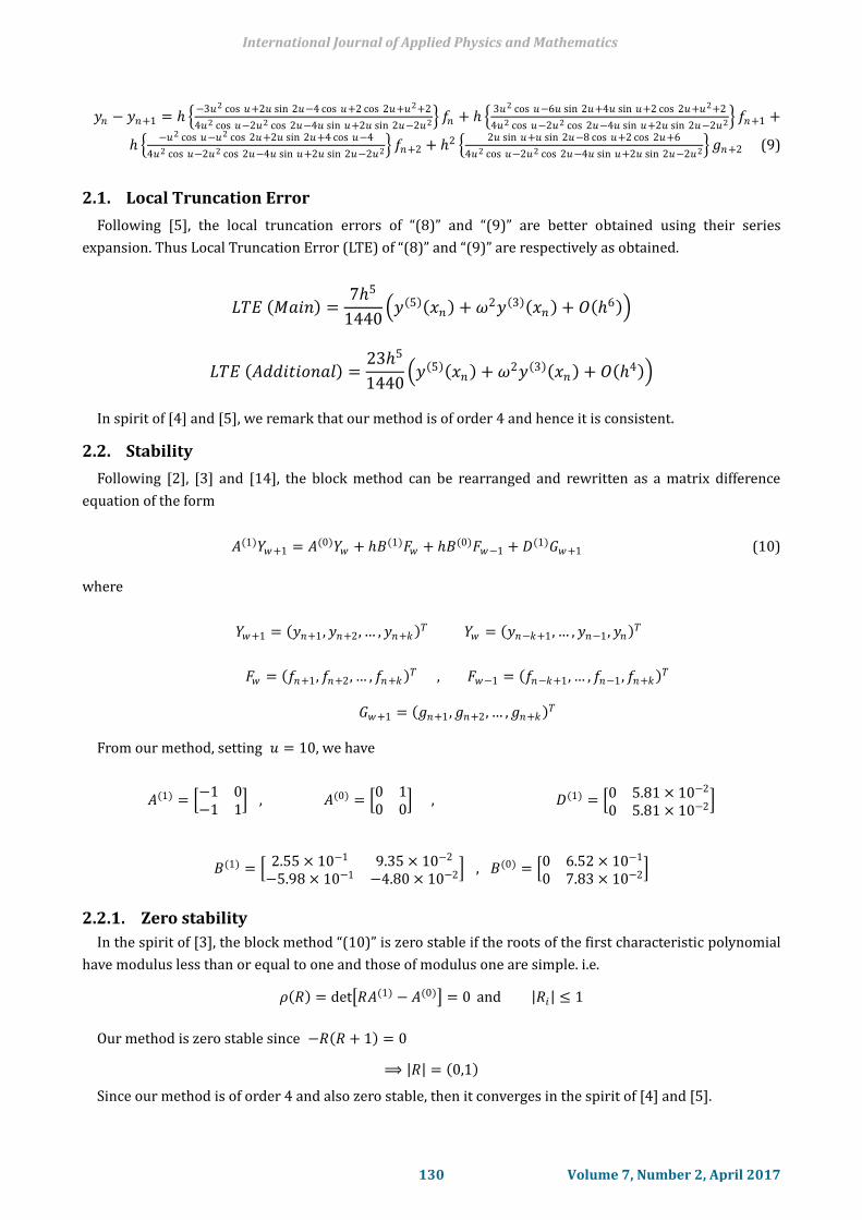
2.2.2. Linear stability
The block method “(10)” applied to the test equations 𝑦′= 𝜆𝑦 and 𝑦′′= 𝜆2𝑦 yields
𝑌𝑤+1 = 𝑀(𝑧)𝑌𝑤
where
𝑀 𝑧 =𝐴(1)−𝑍𝐵 1 −𝑍2𝐷(1)
𝐴(0)+𝑍𝐵(0) (11)
𝑍 = 𝜆
Fig. 1. Region of absolute stability.
The matrix “(11)” has eigenvalues 𝜇1, 𝜇2 = 0, 𝜇2 , where
𝜇2 =−2.10×10³𝑍−3.41×10⁴𝑍2×8.33×104
6.90×10⁴𝑍+5.52×10³𝑍2×8.33×104−4.13×10³𝑍3 (12)
Equation (12) is referred to as the stability function. By employing boundary locus technique, the region
of absolute stability of our method is as shown in figure 1
It is obvious from the RAS that our method is 𝐴0 stable. Also since lim𝑧→∞ 𝜇2 = 0
This shows that our method is 𝐿0 stable.
3. Numerical Examples
In this section, we provide numerical examples both linear and nonlinear autonomous systems to
illustrate the accuracy of our method. All computations are carried out by written codes with the aid of
MAPLE 2015.1 software package. An error of the form 𝑃 × 10−𝑠 is written as 𝑃(−𝑠).
Example 1
We consider the following linear homogeneous Autonomous systems by Sanugi and Evans [8]
𝑦′= 0 −11 0
𝑦 , 𝑦 0 = 10
whose exact solution is
𝑦 = cos 𝑥sin 𝑥
The problem is solve for = 0.1, 𝜔 = 1 in the interval 0 ≤ 𝑥 ≤ 1.
International Journal of Applied Physics and Mathematics
131 Volume 7, Number 2, April 2017
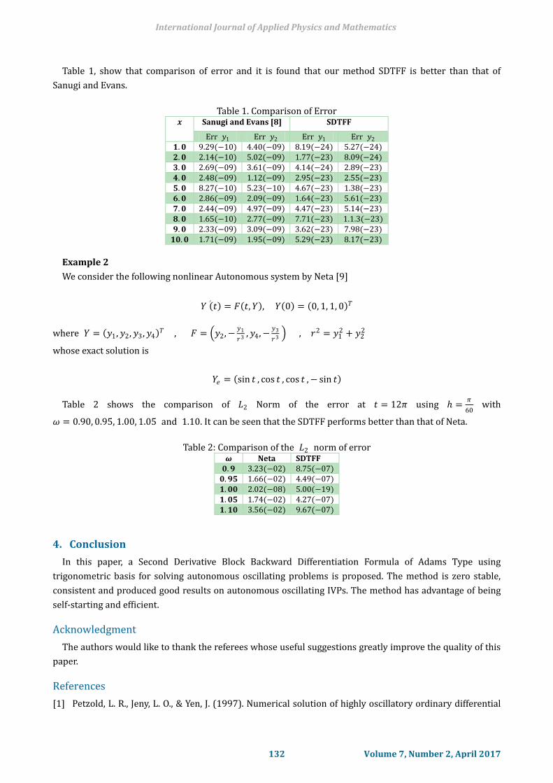
Table 1, show that comparison of error and it is found that our method SDTFF is better than that of
Sanugi and Evans.
Table 1. Comparison of Error
𝒙 Sanugi and Evans [8] SDTFF
Err 𝑦1 Err 𝑦2 Err 𝑦1 Err 𝑦2 𝟏. 𝟎 9.29(−10) 4.40(−09) 8.19(−24) 5.27(−24) 𝟐. 𝟎 2.14(−10) 5.02(−09) 1.77(−23) 8.09(−24) 𝟑. 𝟎 2.69(−09) 3.61(−09) 4.14(−24) 2.89(−23) 𝟒. 𝟎 2.48(−09) 1.12(−09) 2.95(−23) 2.55(−23) 𝟓. 𝟎 8.27(−10) 5.23(−10) 4.67(−23) 1.38(−23) 𝟔. 𝟎 2.86(−09) 2.09(−09) 1.64(−23) 5.61(−23) 𝟕. 𝟎 2.44(−09) 4.97(−09) 4.47(−23) 5.14(−23) 𝟖. 𝟎 1.65(−10) 2.77(−09) 7.71(−23) 1.1.3(−23) 𝟗. 𝟎 2.33(−09) 3.09(−09) 3.62(−23) 7.98(−23) 𝟏𝟎. 𝟎 1.71(−09) 1.95(−09) 5.29(−23) 8.17(−23)
Example 2
We consider the following nonlinear Autonomous system by Neta [9]
𝑌′ 𝑡 = 𝐹 𝑡, 𝑌 , 𝑌 0 = 0, 1, 1, 0 𝑇
where 𝑌 = 𝑦1, 𝑦2, 𝑦3, 𝑦4 𝑇 , 𝐹 = 𝑦2, −𝑦1
𝑟3 , 𝑦4, −𝑦3
𝑟3 , 𝑟2 = 𝑦12 + 𝑦2
2
whose exact solution is
𝑌𝑒 = sin 𝑡 , cos 𝑡 , cos 𝑡 , − sin 𝑡
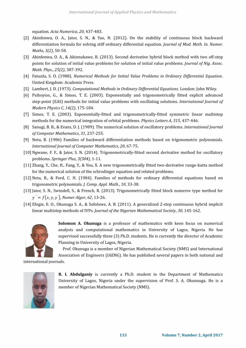
Table 2 shows the comparison of 𝐿2 Norm of the error at 𝑡 = 12𝜋 using =𝜋
60 with
𝜔 = 0.90, 0.95, 1.00, 1.05 and 1.10. It can be seen that the SDTFF performs better than that of Neta.
Table 2: Comparison of the 𝐿2 norm of error
𝝎 Neta SDTFF 𝟎. 𝟗 3.23(−02) 8.75(−07) 𝟎. 𝟗𝟓 1.66(−02) 4.49(−07) 𝟏. 𝟎𝟎 2.02(−08) 5.00(−19) 𝟏. 𝟎𝟓 1.74(−02) 4.27(−07) 𝟏. 𝟏𝟎 3.56(−02) 9.67(−07)
4. Conclusion
In this paper, a Second Derivative Block Backward Differentiation Formula of Adams Type using
trigonometric basis for solving autonomous oscillating problems is proposed. The method is zero stable,
consistent and produced good results on autonomous oscillating IVPs. The method has advantage of being
self-starting and efficient.
Acknowledgment
The authors would like to thank the referees whose useful suggestions greatly improve the quality of this
paper.
References
[1] Petzold, L. R., Jeny, L. O., & Yen, J. (1997). Numerical solution of highly oscillatory ordinary differential
International Journal of Applied Physics and Mathematics
132 Volume 7, Number 2, April 2017
equation. Acta Numerica, 20, 437-483.
[2] Akinfenwa, O. A., Jator, S. N., & Yao, N. (2012). On the stability of continuous block backward
differentiation formula for solving stiff ordinary differential equation. Journal of Mod. Meth. In. Numer.
Maths, 3(2), 50-58.
[3] Akinfenwa, O. A., & Akinnukawe, B. (2013). Second derivative hybrid block method with two off-step
points for solution of initial value problems for solution of initial value problems. Journal of Nig. Assoc.
Math. Phys., 25(2), 387-392.
[4] Fatunla, S. O. (1988). Numerical Methods for Initial Value Problems in Ordinary Differential Equation.
United Kingdom: Academic Press.
[5] Lambert, J. D. (1973). Computational Methods in Ordinary Differential Equations. London: John Wiley.
[6] Psihoyios, G., & Simos, T. E. (2003). Exponentially and trigonometrically fitted explicit advanced
step-point (EAS) methods for initial value problems with oscillating solutions. International Journal of
Modern Physics C, 14(2), 175-184.
[7] Simos, T. E. (2003). Exponentially-fitted and trigonometrically-fitted symmetric linear multistep
methods for the numerical integration of orbital problems. Physics Letters A, 315, 437-446.
[8] Sanugi, B. B., & Evans, D. J. (1989). The numerical solution of oscillatory problems. International Journal
of Computer Mathematics, 31, 237-255.
[9] Neta, B. (1986) Families of backward differentiation methods based on trigonometric polynomials.
International Journal of Computer Mathematics, 20, 67-75.
[10] Ngwane, F. F., & Jator, S. N. (2014). Trigonometrically-fitted second derivative method for oscillatory
problems. Springer Plus, 3(304), 1-11.
[11] Zhang, Y., Che, H., Fang, Y., & You, X. A new trigonometrically fitted two-derivative runge-kutta method
for the numerical solution of the schrodinger equation and related problems.
[12] Neta, B., & Ford, C. H. (1984). Families of methods for ordinary differential equations based on
trigonometric polynomials. J. Comp. Appl. Math., 10, 33-38.
[13] Jator, S. N., Swindell, S., & French, R. (2013). Trigonometrically fitted block numerov type method for
𝑦′′= 𝑓 𝑥, 𝑦, 𝑦′ , Numer Algor, 62, 13-26.
[14] Ehigie, E. O., Okunuga S. A., & Sofoluwe, A. B. (2011). A generalized 2-step continuous hybrid implicit
linear multistep methods of IVPs. Journal of the Nigerian Mathematical Society, 30, 145-162.
R. I. Abdulganiy is currently a Ph.D. student in the Department of Mathematics
University of Lagos, Nigeria under the supervision of Prof. S. A. Okunnuga. He is a
member of Nigerian Mathematical Society (NMS).
International Journal of Applied Physics and Mathematics
133 Volume 7, Number 2, April 2017
Solomon A. Okunuga is a professor of mathematics with keen focus on numerical
analysis and computational mathematics in University of Lagos, Nigeria. He has
supervised successfully three (3) Ph.D. students. He is currently the director of Academic
Planning in University of Lagos, Nigeria.
Prof. Okunuga is a member of Nigerian Mathematical Society (NMS) and International
Association of Engineers (IAENG). He has published several papers in both national and
international journals.