Embed Size (px)
Citation preview
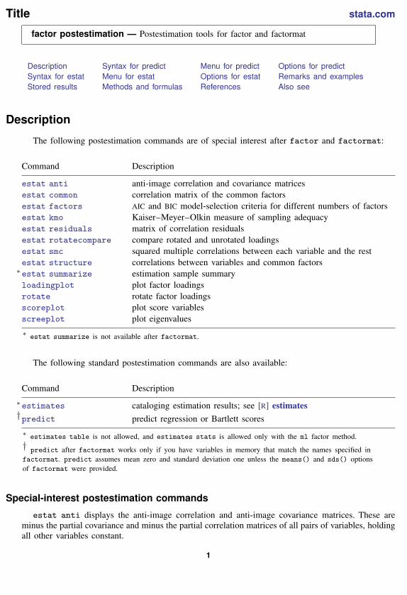
Title stata.com
factor postestimation — Postestimation tools for factor and factormat
Description Syntax for predict Menu for predict Options for predictSyntax for estat Menu for estat Options for estat Remarks and examplesStored results Methods and formulas References Also see
Description
The following postestimation commands are of special interest after factor and factormat:
Command Description
estat anti anti-image correlation and covariance matricesestat common correlation matrix of the common factorsestat factors AIC and BIC model-selection criteria for different numbers of factorsestat kmo Kaiser–Meyer–Olkin measure of sampling adequacyestat residuals matrix of correlation residualsestat rotatecompare compare rotated and unrotated loadingsestat smc squared multiple correlations between each variable and the restestat structure correlations between variables and common factors∗estat summarize estimation sample summaryloadingplot plot factor loadingsrotate rotate factor loadingsscoreplot plot score variablesscreeplot plot eigenvalues
∗ estat summarize is not available after factormat.
The following standard postestimation commands are also available:
Command Description
∗estimates cataloging estimation results; see [R] estimates†predict predict regression or Bartlett scores
∗ estimates table is not allowed, and estimates stats is allowed only with the ml factor method.† predict after factormat works only if you have variables in memory that match the names specified infactormat. predict assumes mean zero and standard deviation one unless the means() and sds() optionsof factormat were provided.
Special-interest postestimation commands
estat anti displays the anti-image correlation and anti-image covariance matrices. These areminus the partial covariance and minus the partial correlation matrices of all pairs of variables, holdingall other variables constant.
1

2 factor postestimation — Postestimation tools for factor and factormat
estat common displays the correlation matrix of the common factors. For orthogonal factorloadings, the common factors are uncorrelated, and hence an identity matrix is shown. estat commonis of more interest after oblique rotations.
estat factors displays model-selection criteria (AIC and BIC) for models with 1, 2, . . . , #factors. Each model is estimated using maximum likelihood (that is, using the ml option of factor).
estat kmo specifies that the Kaiser–Meyer–Olkin (KMO) measure of sampling adequacy bedisplayed. KMO takes values between 0 and 1, with small values meaning that overall the variableshave too little in common to warrant a factor analysis. Historically, the following labels are given tovalues of KMO (Kaiser 1974):
0.00 to 0.49 unacceptable0.50 to 0.59 miserable0.60 to 0.69 mediocre0.70 to 0.79 middling0.80 to 0.89 meritorious0.90 to 1.00 marvelous
estat residuals displays the raw or standardized residuals of the observed correlations withrespect to the fitted (reproduced) correlation matrix.
estat rotatecompare displays the unrotated factor loadings and the most recent rotated factorloadings.
estat smc displays the squared multiple correlations between each variable and all other variables.SMC is a theoretical lower bound for communality, so it is an upper bound for uniqueness. The pffactor method estimates the communalities by smc.
estat structure displays the factor structure, that is, the correlations between the variables andthe common factors.
estat summarize displays summary statistics of the variables in the factor analysis over theestimation sample. This subcommand is, of course, not available after factormat.
rotate modifies the results of the last factor or factormat command to create a set of loadingsthat are more interpretable than those originally produced. A variety of orthogonal and obliquerotations are available, including varimax, orthomax, promax, and oblimin. See [MV] rotate for moredetails. rotate stores results along with the original estimation results so that replaying factor orfactormat and other postestimation commands may refer to the unrotated as well as the rotatedresults.
factor postestimation — Postestimation tools for factor and factormat 3
Syntax for predict
predict[
type]{stub* | newvarlist}
[if] [
in] [
, statistic options]
statistic Description
Main
regression regression scoring methodbartlett Bartlett scoring method
options Description
Main
norotated use unrotated results, even when rotated results are availablenotable suppress table of scoring coefficientsformat(% fmt) format for displaying the scoring coefficients
Menu for predict
Statistics > Postestimation > Predictions, residuals, etc.
Options for predict
� � �Main �
regression produces factors scored by the regression method.
bartlett produces factors scored by the method suggested by Bartlett (1937, 1938). This methodproduces unbiased factors, but they may be less accurate than those produced by the defaultregression method suggested by Thomson (1951). Regression-scored factors have the smallestmean squared error from the true factors but may be biased.
norotated specifies that unrotated factors be scored even when you have previously issued a rotatecommand. The default is to use rotated factors if they are available and unrotated factors otherwise.
notable suppresses the table of scoring coefficients.
format(% fmt) specifies the display format for scoring coefficients.
Syntax for estatAnti-image correlation/covariance matrices
estat anti[, nocorr nocov format(% fmt)
]Correlation of common factors
estat common[, norotated format(% fmt)
]
4 factor postestimation — Postestimation tools for factor and factormat
Model-selection criteria
estat factors[, factors(#) detail
]Sample adequacy measures
estat kmo[, novar format(% fmt)
]Residuals of correlation matrix
estat residuals[, fitted obs sresiduals format(% fmt)
]Comparison of rotated and unrotated loadings
estat rotatecompare[, format(% fmt)
]Squared multiple correlations
estat smc[, format(% fmt)
]Correlations between variables and common factors
estat structure[, norotated format(% fmt)
]Summarize variables for estimation sample
estat summarize[, labels noheader noweights
]Menu for estat
Statistics > Postestimation > Reports and statistics
Options for estat
� � �Main �
nocorr, an option used with estat anti, suppresses the display of the anti-image correlation matrix.
nocov, an option used with estat anti, suppresses the display of the anti-image covariance matrix.
format(% fmt) specifies the display format. The defaults differ between the subcommands.
norotated, an option used with estat common and estat structure, requests that the displayedand returned results be based on the unrotated original factor solution rather than on the lastrotation (orthogonal or oblique).
factors(#), an option used with estat factors, specifies the maximum number of factors toinclude in the summary table.
detail, an option used with estat factors, presents the output from each run of factor (orfactormat) used in the computations of the AIC and BIC values.
novar, an option used with estat kmo, suppresses the KMO measures of sampling adequacy for thevariables in the factor analysis, displaying the overall KMO measure only.
factor postestimation — Postestimation tools for factor and factormat 5
fitted, an option used with estat residuals, displays the fitted (reconstructed) correlation matrixon the basis of the retained factors.
obs, an option used with estat residuals, displays the observed correlation matrix.
sresiduals, an option used with estat residuals, displays the matrix of standardized residualsof the correlations. Be careful when interpreting these residuals; see Joreskog and Sorbom (1988).
labels, noheader, and noweights are the same as for the generic estat summarize command;see [R] estat summarize.
Remarks and examples stata.com
Remarks are presented under the following headings:
Postestimation statisticsPlots of eigenvalues, factor loadings, and scoresRotating the factor loadingsFactor scores
Postestimation statistics
Many postestimation statistics are available after factor and factormat.
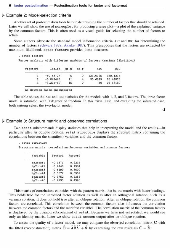
Example 1: Squared multiple correlations
After factor and factormat there are several “classical” methods for assessing whether thevariables have enough in common to have warranted the use of a factor model. One method is toexamine the squared multiple correlations of each variable with all other variables—this is usuallyan upper bound to communality and thus a lower bound to 1− uniqueness(= communality) of thevariables.
. use http://www.stata-press.com/data/r13/bg2(Physician-cost data)
. quietly factor bg2cost1-bg2cost6, factors(2) ml
. estat smc
Squared multiple correlations of variables with all other variables
Variable smc
bg2cost1 0.1054bg2cost2 0.1370bg2cost3 0.1637bg2cost4 0.0866bg2cost5 0.1671bg2cost6 0.1683
Other diagnostic tools, such as examining the anti-image correlation and anti-image covariancematrices (estat anti) and the Kaiser–Meyer–Olkin measure of sampling adequacy (estat kmo),are also available. See [MV] pca postestimation for an illustration of their use.
6 factor postestimation — Postestimation tools for factor and factormat
Example 2: Model-selection criteria
Another set of postestimation tools help in determining the number of factors that should be retained.Later we will show the use of screeplot for producing a scree plot—a plot of the explained varianceby the common factors. This is often used as a visual guide for selecting the number of factors toretain.
Some authors advocate the standard model information criteria AIC and BIC for determining thenumber of factors (Schwarz 1978; Akaike 1987). This presupposes that the factors are extracted bymaximum likelihood. estat factors provides these measures.
. estat factors
Factor analysis with different numbers of factors (maximum likelihood)
#factors loglik df_m df_r AIC BIC
1 -60.53727 6 9 133.0745 159.12732 -6.842448 11 4 35.6849 83.448233 -3.37e-12 15 0 30 95.13182
no Heywood cases encountered
The table shows the AIC and BIC statistics for the models with 1, 2, and 3 factors. The three-factormodel is saturated, with 0 degrees of freedom. In this trivial case, and excluding the saturated case,both criteria select the two-factor model.
Example 3: Structure matrix and observed correlations
Two estat subcommands display statistics that help in interpreting the model and the results—inparticular after an oblique rotation. estat structure displays the structure matrix containing thecorrelations between the (manifest) variables and the common factors.
. estat structure
Structure matrix: correlations between variables and common factors
Variable Factor1 Factor2
bg2cost1 -0.1371 0.4235bg2cost2 0.4140 0.1994bg2cost3 0.6199 0.3692bg2cost4 0.3577 0.0909bg2cost5 -0.3752 0.4355bg2cost6 -0.4295 0.4395
This matrix of correlations coincides with the pattern matrix, that is, the matrix with factor loadings.This holds true for the unrotated factor solution as well as after an orthogonal rotation, such as avarimax rotation. It does not hold true after an oblique rotation. After an oblique rotation, the commonfactors are correlated. This correlation between the common factors also influences the correlationbetween the common factors and the manifest variables. The correlation matrix of the common factorsis displayed by the common subcommand of estat. Because we have not yet rotated, we would seeonly an identity matrix. Later we show estat common output after an oblique rotation.
To assess the quality of a factor model, we may compare the observed correlation matrix C withthe fitted (“reconstructed”) matrix Σ = ΛΦΛ
′+ Ψ by examining the raw residuals C− Σ.
factor postestimation — Postestimation tools for factor and factormat 7
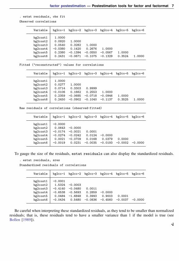
. estat residuals, obs fit
Observed correlations
Variable bg2co~1 bg2co~2 bg2co~3 bg2co~4 bg2co~5 bg2co~6
bg2cost1 1.0000bg2cost2 0.0920 1.0000bg2cost3 0.0540 0.3282 1.0000bg2cost4 -0.0380 0.1420 0.2676 1.0000bg2cost5 0.2380 -0.1394 -0.0550 -0.0567 1.0000bg2cost6 0.2431 -0.0671 -0.1075 -0.1329 0.3524 1.0000
Fitted ("reconstructed") values for correlations
Variable bg2co~1 bg2co~2 bg2co~3 bg2co~4 bg2co~5 bg2co~6
bg2cost1 1.0000bg2cost2 0.0277 1.0000bg2cost3 0.0714 0.3303 0.9999bg2cost4 -0.0106 0.1662 0.2553 1.0000bg2cost5 0.2359 -0.0685 -0.0718 -0.0946 1.0000bg2cost6 0.2450 -0.0902 -0.1040 -0.1137 0.3525 1.0000
Raw residuals of correlations (observed-fitted)
Variable bg2co~1 bg2co~2 bg2co~3 bg2co~4 bg2co~5 bg2co~6
bg2cost1 -0.0000bg2cost2 0.0643 -0.0000bg2cost3 -0.0174 -0.0021 0.0001bg2cost4 -0.0274 -0.0242 0.0124 -0.0000bg2cost5 0.0021 -0.0709 0.0168 0.0379 0.0000bg2cost6 -0.0019 0.0231 -0.0035 -0.0193 -0.0002 -0.0000
To gauge the size of the residuals, estat residuals can also display the standardized residuals.
. estat residuals, sres
Standardized residuals of correlations
Variable bg2co~1 bg2co~2 bg2co~3 bg2co~4 bg2co~5 bg2co~6
bg2cost1 -0.0001bg2cost2 1.5324 -0.0003bg2cost3 -0.4140 -0.0480 0.0011bg2cost4 -0.6538 -0.5693 0.2859 -0.0000bg2cost5 0.0484 -1.6848 0.3993 0.9003 0.0001bg2cost6 -0.0434 0.5480 -0.0836 -0.4560 -0.0037 -0.0000
Be careful when interpreting these standardized residuals, as they tend to be smaller than normalizedresiduals; that is, these residuals tend to have a smaller variance than 1 if the model is true (seeBollen [1989]).
8 factor postestimation — Postestimation tools for factor and factormat
Plots of eigenvalues, factor loadings, and scores
Scree plots, factor loading plots, and score plots are easily obtained after factor and factormat.
Example 4: The scree plot
The scree plot is a popular tool for determining the number of factors to be retained. A screeplot is a plot of the eigenvalues shown in decreasing order (Cattell 1966). We fit a factor model,extracting factors with the principal factor method.
. use http://www.stata-press.com/data/r13/sp2
. factor ghp31-ghp05, pcf(output omitted )
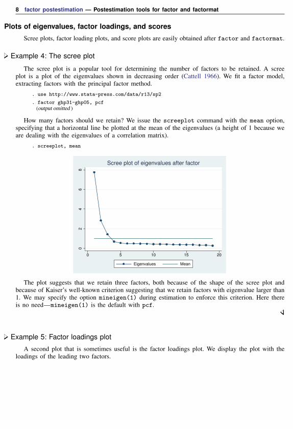
How many factors should we retain? We issue the screeplot command with the mean option,specifying that a horizontal line be plotted at the mean of the eigenvalues (a height of 1 because weare dealing with the eigenvalues of a correlation matrix).
. screeplot, mean
02
46
8
0 5 10 15 20
Eigenvalues Mean
Scree plot of eigenvalues after factor
The plot suggests that we retain three factors, both because of the shape of the scree plot andbecause of Kaiser’s well-known criterion suggesting that we retain factors with eigenvalue larger than1. We may specify the option mineigen(1) during estimation to enforce this criterion. Here thereis no need—mineigen(1) is the default with pcf.
Example 5: Factor loadings plot
A second plot that is sometimes useful is the factor loadings plot. We display the plot with theloadings of the leading two factors.
factor postestimation — Postestimation tools for factor and factormat 9
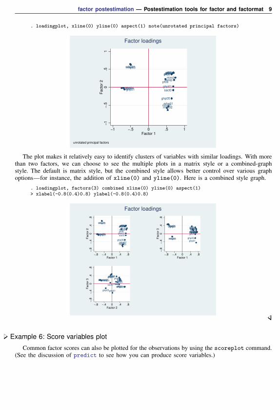
. loadingplot, xline(0) yline(0) aspect(1) note(unrotated principal factors)
ghp31
pf01pf02pf03pf04pf05
pf06rkeep
rkind
sact0
mha01
mhp03
mhd02
mhp01
mhc01
ghp01ghp04ghp02
ghp05
−1
−.5
0.5
1F
acto
r 2
−1 −.5 0 .5 1Factor 1
unrotated principal factors
Factor loadings
The plot makes it relatively easy to identify clusters of variables with similar loadings. With morethan two factors, we can choose to see the multiple plots in a matrix style or a combined-graphstyle. The default is matrix style, but the combined style allows better control over various graphoptions—for instance, the addition of xline(0) and yline(0). Here is a combined style graph.
. loadingplot, factors(3) combined xline(0) yline(0) aspect(1)> xlabel(-0.8(0.4)0.8) ylabel(-0.8(0.4)0.8)
ghp31
pf01pf02pf03pf04pf05
pf06rkeep
rkind
sact0
mha01
mhp03
mhd02
mhp01
mhc01
ghp01ghp04ghp02
ghp05
−.8
−.4
0.4
.8F
acto
r 2
−.8 −.4 0 .4 .8Factor 1
ghp31
pf01
pf02pf03pf04pf05pf06
rkeeprkindsact0mha01
mhp03
mhd02
mhp01
mhc01
ghp01
ghp04ghp02
ghp05
−.8
−.4
0.4
.8F
acto
r 3
−.8 −.4 0 .4 .8Factor 1
ghp31
pf01
pf02pf03pf04pf05pf06
rkeeprkindsact0
mha01
mhp03
mhd02
mhp01
mhc01
ghp01
ghp04ghp02
ghp05
−.8
−.4
0.4
.8F
acto
r 3
−.8 −.4 0 .4 .8Factor 2
Factor loadings
Example 6: Score variables plot
Common factor scores can also be plotted for the observations by using the scoreplot command.(See the discussion of predict to see how you can produce score variables.)
10 factor postestimation — Postestimation tools for factor and factormat
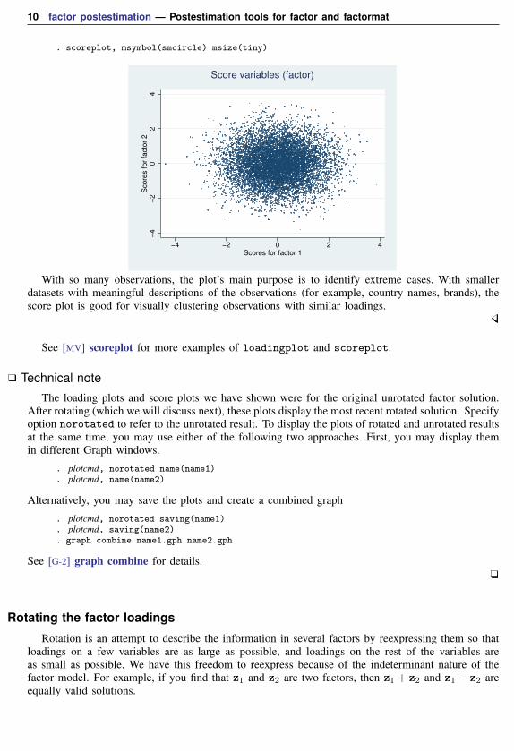
. scoreplot, msymbol(smcircle) msize(tiny)
−4
−2
02
4S
co
res f
or
facto
r 2
−4 −2 0 2 4Scores for factor 1
Score variables (factor)
With so many observations, the plot’s main purpose is to identify extreme cases. With smallerdatasets with meaningful descriptions of the observations (for example, country names, brands), thescore plot is good for visually clustering observations with similar loadings.
See [MV] scoreplot for more examples of loadingplot and scoreplot.
Technical note
The loading plots and score plots we have shown were for the original unrotated factor solution.After rotating (which we will discuss next), these plots display the most recent rotated solution. Specifyoption norotated to refer to the unrotated result. To display the plots of rotated and unrotated resultsat the same time, you may use either of the following two approaches. First, you may display themin different Graph windows.
. plotcmd, norotated name(name1)
. plotcmd, name(name2)
Alternatively, you may save the plots and create a combined graph
. plotcmd, norotated saving(name1)
. plotcmd, saving(name2)
. graph combine name1.gph name2.gph
See [G-2] graph combine for details.
Rotating the factor loadings
Rotation is an attempt to describe the information in several factors by reexpressing them so thatloadings on a few variables are as large as possible, and loadings on the rest of the variables areas small as possible. We have this freedom to reexpress because of the indeterminant nature of thefactor model. For example, if you find that z1 and z2 are two factors, then z1 + z2 and z1 − z2 areequally valid solutions.

factor postestimation — Postestimation tools for factor and factormat 11
Technical note
Said more technically: we are trying to find a set of f factor variables such that the observedvariables can be best explained by regressing them on the f factor variables. Usually, f is a smallnumber such as 1 or 2. If f ≥ 2, there is an inherent indeterminacy in the construction of the factorsbecause any linear combination of the calculated factors serves equally well as a set of regressors.Rotation capitalizes on this indeterminacy to create a set of variables that looks as much like theoriginal variables as possible.
The rotate command modifies the results of the last factor or factormat command to createa set of loadings that are more interpretable than those produced by factor or factormat. Youmay perform one factor analysis followed by several rotate commands, thus experimenting withdifferent types of rotation. If you retain too few factors, the variables for several distinct conceptsmay be merged, as in our example below. If you retain too many factors, several factors may attemptto measure the same concept, causing the factors to get in each other’s way, suggesting too manydistinct concepts after rotation.
Technical note
It is possible to restrict rotation to a number of leading factors. For instance, if you extracted threefactors, you may specify the option factors(2) to rotate to exclude the third factor from beingrotated. The new two leading factors are combinations of the initial two leading factors and are notaffected by the fixed factor.
12 factor postestimation — Postestimation tools for factor and factormat
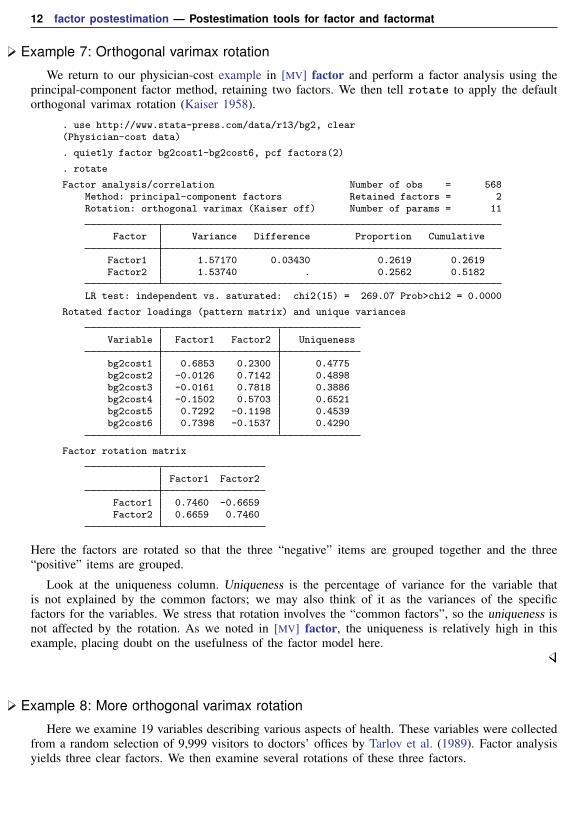
Example 7: Orthogonal varimax rotation
We return to our physician-cost example in [MV] factor and perform a factor analysis using theprincipal-component factor method, retaining two factors. We then tell rotate to apply the defaultorthogonal varimax rotation (Kaiser 1958).
. use http://www.stata-press.com/data/r13/bg2, clear(Physician-cost data)
. quietly factor bg2cost1-bg2cost6, pcf factors(2)
. rotate
Factor analysis/correlation Number of obs = 568Method: principal-component factors Retained factors = 2Rotation: orthogonal varimax (Kaiser off) Number of params = 11
Factor Variance Difference Proportion Cumulative
Factor1 1.57170 0.03430 0.2619 0.2619Factor2 1.53740 . 0.2562 0.5182
LR test: independent vs. saturated: chi2(15) = 269.07 Prob>chi2 = 0.0000
Rotated factor loadings (pattern matrix) and unique variances
Variable Factor1 Factor2 Uniqueness
bg2cost1 0.6853 0.2300 0.4775bg2cost2 -0.0126 0.7142 0.4898bg2cost3 -0.0161 0.7818 0.3886bg2cost4 -0.1502 0.5703 0.6521bg2cost5 0.7292 -0.1198 0.4539bg2cost6 0.7398 -0.1537 0.4290
Factor rotation matrix
Factor1 Factor2
Factor1 0.7460 -0.6659Factor2 0.6659 0.7460
Here the factors are rotated so that the three “negative” items are grouped together and the three“positive” items are grouped.
Look at the uniqueness column. Uniqueness is the percentage of variance for the variable thatis not explained by the common factors; we may also think of it as the variances of the specificfactors for the variables. We stress that rotation involves the “common factors”, so the uniqueness isnot affected by the rotation. As we noted in [MV] factor, the uniqueness is relatively high in thisexample, placing doubt on the usefulness of the factor model here.
Example 8: More orthogonal varimax rotation
Here we examine 19 variables describing various aspects of health. These variables were collectedfrom a random selection of 9,999 visitors to doctors’ offices by Tarlov et al. (1989). Factor analysisyields three clear factors. We then examine several rotations of these three factors.
factor postestimation — Postestimation tools for factor and factormat 13
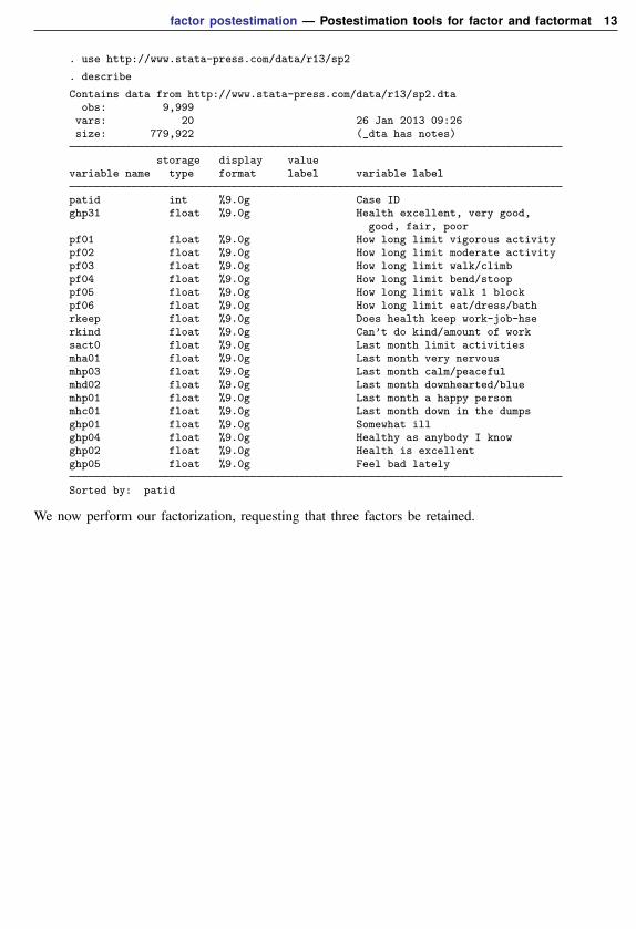
. use http://www.stata-press.com/data/r13/sp2
. describe
Contains data from http://www.stata-press.com/data/r13/sp2.dtaobs: 9,999
vars: 20 26 Jan 2013 09:26size: 779,922 (_dta has notes)
storage display valuevariable name type format label variable label
patid int %9.0g Case IDghp31 float %9.0g Health excellent, very good,
good, fair, poorpf01 float %9.0g How long limit vigorous activitypf02 float %9.0g How long limit moderate activitypf03 float %9.0g How long limit walk/climbpf04 float %9.0g How long limit bend/stooppf05 float %9.0g How long limit walk 1 blockpf06 float %9.0g How long limit eat/dress/bathrkeep float %9.0g Does health keep work-job-hserkind float %9.0g Can’t do kind/amount of worksact0 float %9.0g Last month limit activitiesmha01 float %9.0g Last month very nervousmhp03 float %9.0g Last month calm/peacefulmhd02 float %9.0g Last month downhearted/bluemhp01 float %9.0g Last month a happy personmhc01 float %9.0g Last month down in the dumpsghp01 float %9.0g Somewhat illghp04 float %9.0g Healthy as anybody I knowghp02 float %9.0g Health is excellentghp05 float %9.0g Feel bad lately
Sorted by: patid
We now perform our factorization, requesting that three factors be retained.
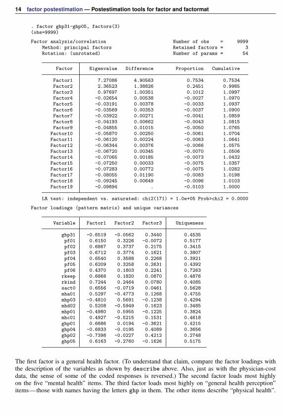
14 factor postestimation — Postestimation tools for factor and factormat
. factor ghp31-ghp05, factors(3)(obs=9999)
Factor analysis/correlation Number of obs = 9999Method: principal factors Retained factors = 3Rotation: (unrotated) Number of params = 54
Factor Eigenvalue Difference Proportion Cumulative
Factor1 7.27086 4.90563 0.7534 0.7534Factor2 2.36523 1.38826 0.2451 0.9985Factor3 0.97697 1.00351 0.1012 1.0997Factor4 -0.02654 0.00538 -0.0027 1.0970Factor5 -0.03191 0.00378 -0.0033 1.0937Factor6 -0.03569 0.00353 -0.0037 1.0900Factor7 -0.03922 0.00271 -0.0041 1.0859Factor8 -0.04193 0.00662 -0.0043 1.0815Factor9 -0.04855 0.01015 -0.0050 1.0765
Factor10 -0.05870 0.00250 -0.0061 1.0704Factor11 -0.06120 0.00224 -0.0063 1.0641Factor12 -0.06344 0.00376 -0.0066 1.0575Factor13 -0.06720 0.00345 -0.0070 1.0506Factor14 -0.07065 0.00185 -0.0073 1.0432Factor15 -0.07250 0.00033 -0.0075 1.0357Factor16 -0.07283 0.00772 -0.0075 1.0282Factor17 -0.08055 0.01190 -0.0083 1.0198Factor18 -0.09245 0.00649 -0.0096 1.0103Factor19 -0.09894 . -0.0103 1.0000
LR test: independent vs. saturated: chi2(171) = 1.0e+05 Prob>chi2 = 0.0000
Factor loadings (pattern matrix) and unique variances
Variable Factor1 Factor2 Factor3 Uniqueness
ghp31 -0.6519 -0.0562 0.3440 0.4535pf01 0.6150 0.3226 -0.0072 0.5177pf02 0.6867 0.3737 0.2175 0.3415pf03 0.6712 0.3774 0.1621 0.3807pf04 0.6540 0.3588 0.2268 0.3921pf05 0.6209 0.3258 0.2631 0.4392pf06 0.4370 0.1803 0.2241 0.7263
rkeep 0.6868 0.1820 0.0870 0.4876rkind 0.7244 0.2464 0.0780 0.4085sact0 0.6556 -0.0719 0.0461 0.5628mha01 0.5297 -0.4773 0.1268 0.4755mhp03 -0.4810 0.5691 -0.1238 0.4294mhd02 0.5208 -0.5949 0.1623 0.3485mhp01 -0.4980 0.5955 -0.1225 0.3824mhc01 0.4927 -0.5215 0.1531 0.4618ghp01 0.6686 0.0194 -0.3621 0.4215ghp04 -0.6833 -0.0195 0.4089 0.3656ghp02 -0.7398 -0.0227 0.4212 0.2748ghp05 0.6163 -0.2760 -0.1626 0.5175
The first factor is a general health factor. (To understand that claim, compare the factor loadings withthe description of the variables as shown by describe above. Also, just as with the physician-costdata, the sense of some of the coded responses is reversed.) The second factor loads most highlyon the five “mental health” items. The third factor loads most highly on “general health perception”items—those with names having the letters ghp in them. The other items describe “physical health”.

factor postestimation — Postestimation tools for factor and factormat 15
These designations are based primarily on the wording of the questions, which is summarized in thevariable labels.
. rotate, varimax
Factor analysis/correlation Number of obs = 9999Method: principal factors Retained factors = 3Rotation: orthogonal varimax (Kaiser off) Number of params = 54
Factor Variance Difference Proportion Cumulative
Factor1 4.20556 0.83302 0.4358 0.4358Factor2 3.37253 0.33756 0.3495 0.7852Factor3 3.03497 . 0.3145 1.0997
LR test: independent vs. saturated: chi2(171) = 1.0e+05 Prob>chi2 = 0.0000
Rotated factor loadings (pattern matrix) and unique variances
Variable Factor1 Factor2 Factor3 Uniqueness
ghp31 -0.2968 -0.1647 -0.6567 0.4535pf01 0.5872 0.0263 0.3699 0.5177pf02 0.7740 0.0848 0.2287 0.3415pf03 0.7386 0.0580 0.2654 0.3807pf04 0.7484 0.0842 0.2018 0.3921pf05 0.7256 0.1063 0.1518 0.4392pf06 0.5023 0.1268 0.0730 0.7263
rkeep 0.6023 0.2048 0.3282 0.4876rkind 0.6590 0.1669 0.3597 0.4085sact0 0.4187 0.3875 0.3342 0.5628mha01 0.1467 0.6859 0.1803 0.4755mhp03 -0.0613 -0.7375 -0.1514 0.4294mhd02 0.0921 0.7893 0.1416 0.3485mhp01 -0.0570 -0.7671 -0.1612 0.3824mhc01 0.1102 0.7124 0.1359 0.4618ghp01 0.2783 0.1977 0.6797 0.4215ghp04 -0.2652 -0.1908 -0.7264 0.3656ghp02 -0.2986 -0.2116 -0.7690 0.2748ghp05 0.1755 0.4756 0.4748 0.5175
Factor rotation matrix
Factor1 Factor2 Factor3
Factor1 0.6658 0.4796 0.5715Factor2 0.5620 -0.8263 0.0387Factor3 0.4908 0.2954 -0.8197
With rotation, the structure of the data becomes much clearer. The first rotated factor is physicalhealth, the second is mental health, and the third is general health perception. The a priori designationof the items is confirmed.
After rotation, physical health is the first factor. rotate has ordered the factors by explainedvariance. Still, we warn that the importance of any factor must be gauged against the number ofvariables that purportedly measure it. Here we included nine variables that measured physical health,five that measured mental health, and five that measured general health perception. Had we startedwith only one mental health item, it would have had a high uniqueness, but we would not want toconclude that it was, therefore, largely noise.

16 factor postestimation — Postestimation tools for factor and factormat
Technical noteSome people prefer specifying the option normalize to apply a Kaiser normalization (Horst 1965),
which places equal weight on all rows of the matrix to be rotated.
Example 9: Oblique oblimin rotation
The literature suggests that physical health and mental health are related. Also, general healthperception may be largely a combination of the two. For these reasons, an oblique rotation of atwo-factor solution is worth trying. We try the oblique oblimin rotation (Harman 1976).
. factor ghp31-ghp05, factors(2)(obs=9999)
Factor analysis/correlation Number of obs = 9999Method: principal factors Retained factors = 2Rotation: (unrotated) Number of params = 37
Factor Eigenvalue Difference Proportion Cumulative
Factor1 7.27086 4.90563 0.7534 0.7534Factor2 2.36523 1.38826 0.2451 0.9985Factor3 0.97697 1.00351 0.1012 1.0997Factor4 -0.02654 0.00538 -0.0027 1.0970Factor5 -0.03191 0.00378 -0.0033 1.0937Factor6 -0.03569 0.00353 -0.0037 1.0900Factor7 -0.03922 0.00271 -0.0041 1.0859Factor8 -0.04193 0.00662 -0.0043 1.0815Factor9 -0.04855 0.01015 -0.0050 1.0765
Factor10 -0.05870 0.00250 -0.0061 1.0704Factor11 -0.06120 0.00224 -0.0063 1.0641Factor12 -0.06344 0.00376 -0.0066 1.0575Factor13 -0.06720 0.00345 -0.0070 1.0506Factor14 -0.07065 0.00185 -0.0073 1.0432Factor15 -0.07250 0.00033 -0.0075 1.0357Factor16 -0.07283 0.00772 -0.0075 1.0282Factor17 -0.08055 0.01190 -0.0083 1.0198Factor18 -0.09245 0.00649 -0.0096 1.0103Factor19 -0.09894 . -0.0103 1.0000
LR test: independent vs. saturated: chi2(171) = 1.0e+05 Prob>chi2 = 0.0000

factor postestimation — Postestimation tools for factor and factormat 17
Factor loadings (pattern matrix) and unique variances
Variable Factor1 Factor2 Uniqueness
ghp31 -0.6519 -0.0562 0.5718pf01 0.6150 0.3226 0.5178pf02 0.6867 0.3737 0.3888pf03 0.6712 0.3774 0.4070pf04 0.6540 0.3588 0.4435pf05 0.6209 0.3258 0.5084pf06 0.4370 0.1803 0.7765
rkeep 0.6868 0.1820 0.4952rkind 0.7244 0.2464 0.4145sact0 0.6556 -0.0719 0.5650mha01 0.5297 -0.4773 0.4916mhp03 -0.4810 0.5691 0.4448mhd02 0.5208 -0.5949 0.3748mhp01 -0.4980 0.5955 0.3974mhc01 0.4927 -0.5215 0.4853ghp01 0.6686 0.0194 0.5526ghp04 -0.6833 -0.0195 0.5327ghp02 -0.7398 -0.0227 0.4522ghp05 0.6163 -0.2760 0.5439
. rotate, oblimin oblique
Factor analysis/correlation Number of obs = 9999Method: principal factors Retained factors = 2Rotation: oblique oblimin (Kaiser off) Number of params = 37
Factor Variance Proportion Rotated factors are correlated
Factor1 6.58719 0.6826Factor2 4.65444 0.4823
LR test: independent vs. saturated: chi2(171) = 1.0e+05 Prob>chi2 = 0.0000
Rotated factor loadings (pattern matrix) and unique variances
Variable Factor1 Factor2 Uniqueness
ghp31 -0.5517 -0.2051 0.5718pf01 0.7179 -0.0747 0.5178pf02 0.8115 -0.0968 0.3888pf03 0.8022 -0.1068 0.4070pf04 0.7750 -0.0951 0.4435pf05 0.7249 -0.0756 0.5084pf06 0.4743 -0.0044 0.7765
rkeep 0.6712 0.0939 0.4952rkind 0.7478 0.0449 0.4145sact0 0.4608 0.3340 0.5650mha01 0.0652 0.6869 0.4916mhp03 0.0401 -0.7587 0.4448mhd02 -0.0280 0.8003 0.3748mhp01 0.0462 -0.7918 0.3974mhc01 0.0039 0.7160 0.4853ghp01 0.5378 0.2484 0.5526ghp04 -0.5494 -0.2541 0.5327ghp02 -0.5960 -0.2736 0.4522ghp05 0.2805 0.5213 0.5439
18 factor postestimation — Postestimation tools for factor and factormat
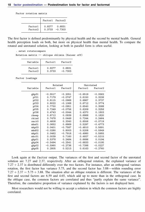
Factor rotation matrix
Factor1 Factor2
Factor1 0.9277 0.6831Factor2 0.3733 -0.7303
The first factor is defined predominantly by physical health and the second by mental health. Generalhealth perception loads on both, but more on physical health than mental health. To compare therotated and unrotated solution, looking at both in parallel form is often useful.
. estat rotatecompare
Rotation matrix oblique oblimin (Kaiser off)
Variable Factor1 Factor2
Factor1 0.9277 0.6831Factor2 0.3733 -0.7303
Factor loadings
Rotated UnrotatedVariable Factor1 Factor2 Factor1 Factor2
ghp31 -0.5517 -0.2051 -0.6519 -0.0562pf01 0.7179 -0.0747 0.6150 0.3226pf02 0.8115 -0.0968 0.6867 0.3737pf03 0.8022 -0.1068 0.6712 0.3774pf04 0.7750 -0.0951 0.6540 0.3588pf05 0.7249 -0.0756 0.6209 0.3258pf06 0.4743 -0.0044 0.4370 0.1803
rkeep 0.6712 0.0939 0.6868 0.1820rkind 0.7478 0.0449 0.7244 0.2464sact0 0.4608 0.3340 0.6556 -0.0719mha01 0.0652 0.6869 0.5297 -0.4773mhp03 0.0401 -0.7587 -0.4810 0.5691mhd02 -0.0280 0.8003 0.5208 -0.5949mhp01 0.0462 -0.7918 -0.4980 0.5955mhc01 0.0039 0.7160 0.4927 -0.5215ghp01 0.5378 0.2484 0.6686 0.0194ghp04 -0.5494 -0.2541 -0.6833 -0.0195ghp02 -0.5960 -0.2736 -0.7398 -0.0227ghp05 0.2805 0.5213 0.6163 -0.2760
Look again at the factor output. The variances of the first and second factor of the unrotatedsolution are 7.27 and 2.37, respectively. After an orthogonal rotation, the explained variance of7.27 + 2.37 is distributed differently over the two factors. For instance, after an orthogonal varimaxrotation, the first factor has variance 5.75, and the second factor has 3.88—within rounding error7.27 + 2.37 = 5.75 + 3.88. The situation after an oblique rotation is different. The variances of thefirst and second factors are 6.59 and 4.65, which add up to more than in the orthogonal case. Inthe oblique case, the common factors are correlated and thus “partly explain the same variance”.Therefore, the cumulative proportion of variance explained by the factors is not displayed here.
Most researchers would not be willing to accept a solution in which the common factors are highlycorrelated.
factor postestimation — Postestimation tools for factor and factormat 19
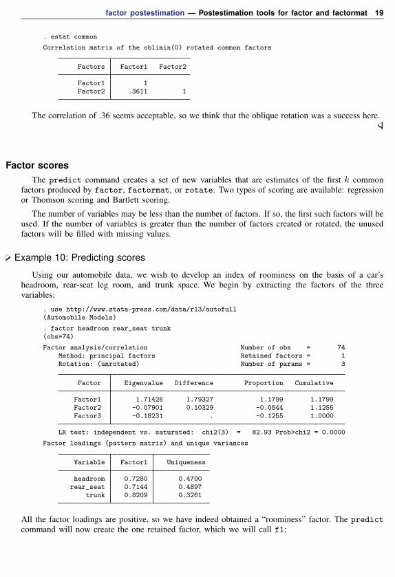
. estat common
Correlation matrix of the oblimin(0) rotated common factors
Factors Factor1 Factor2
Factor1 1Factor2 .3611 1
The correlation of .36 seems acceptable, so we think that the oblique rotation was a success here.
Factor scoresThe predict command creates a set of new variables that are estimates of the first k common
factors produced by factor, factormat, or rotate. Two types of scoring are available: regressionor Thomson scoring and Bartlett scoring.
The number of variables may be less than the number of factors. If so, the first such factors will beused. If the number of variables is greater than the number of factors created or rotated, the unusedfactors will be filled with missing values.
Example 10: Predicting scores
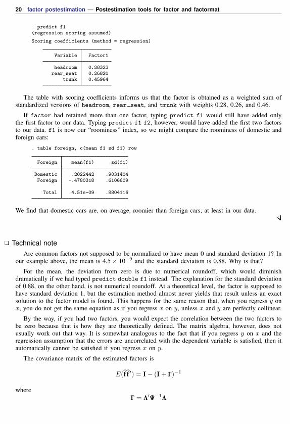
Using our automobile data, we wish to develop an index of roominess on the basis of a car’sheadroom, rear-seat leg room, and trunk space. We begin by extracting the factors of the threevariables:
. use http://www.stata-press.com/data/r13/autofull(Automobile Models)
. factor headroom rear_seat trunk(obs=74)
Factor analysis/correlation Number of obs = 74Method: principal factors Retained factors = 1Rotation: (unrotated) Number of params = 3
Factor Eigenvalue Difference Proportion Cumulative
Factor1 1.71426 1.79327 1.1799 1.1799Factor2 -0.07901 0.10329 -0.0544 1.1255Factor3 -0.18231 . -0.1255 1.0000
LR test: independent vs. saturated: chi2(3) = 82.93 Prob>chi2 = 0.0000
Factor loadings (pattern matrix) and unique variances
Variable Factor1 Uniqueness
headroom 0.7280 0.4700rear_seat 0.7144 0.4897
trunk 0.8209 0.3261
All the factor loadings are positive, so we have indeed obtained a “roominess” factor. The predictcommand will now create the one retained factor, which we will call f1:
20 factor postestimation — Postestimation tools for factor and factormat
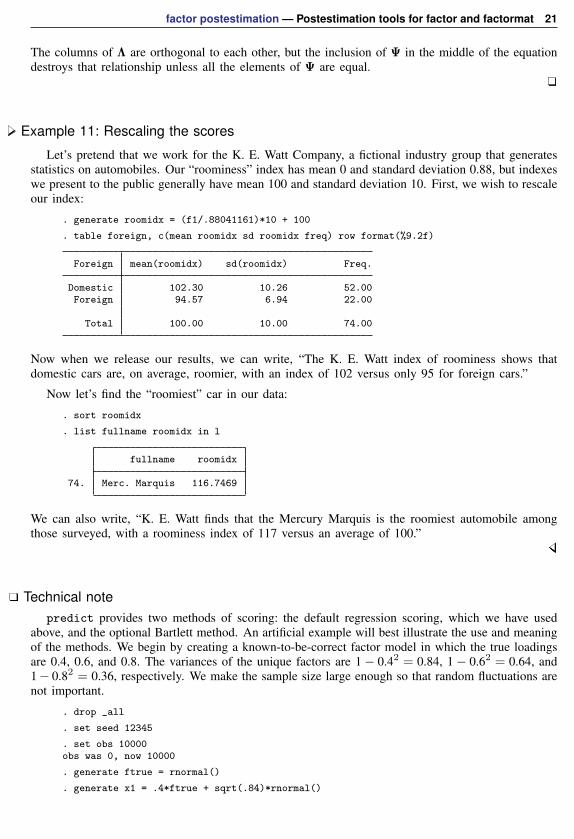
. predict f1(regression scoring assumed)
Scoring coefficients (method = regression)
Variable Factor1
headroom 0.28323rear_seat 0.26820
trunk 0.45964
The table with scoring coefficients informs us that the factor is obtained as a weighted sum ofstandardized versions of headroom, rear seat, and trunk with weights 0.28, 0.26, and 0.46.
If factor had retained more than one factor, typing predict f1 would still have added onlythe first factor to our data. Typing predict f1 f2, however, would have added the first two factorsto our data. f1 is now our “roominess” index, so we might compare the roominess of domestic andforeign cars:
. table foreign, c(mean f1 sd f1) row
Foreign mean(f1) sd(f1)
Domestic .2022442 .9031404Foreign -.4780318 .6106609
Total 4.51e-09 .8804116
We find that domestic cars are, on average, roomier than foreign cars, at least in our data.
Technical noteAre common factors not supposed to be normalized to have mean 0 and standard deviation 1? In
our example above, the mean is 4.5× 10⁻⁹ and the standard deviation is 0.88. Why is that?
For the mean, the deviation from zero is due to numerical roundoff, which would diminishdramatically if we had typed predict double f1 instead. The explanation for the standard deviationof 0.88, on the other hand, is not numerical roundoff. At a theoretical level, the factor is supposed tohave standard deviation 1, but the estimation method almost never yields that result unless an exactsolution to the factor model is found. This happens for the same reason that, when you regress y onx, you do not get the same equation as if you regress x on y, unless x and y are perfectly collinear.
By the way, if you had two factors, you would expect the correlation between the two factors tobe zero because that is how they are theoretically defined. The matrix algebra, however, does notusually work out that way. It is somewhat analogous to the fact that if you regress y on x and theregression assumption that the errors are uncorrelated with the dependent variable is satisfied, then itautomatically cannot be satisfied if you regress x on y.
The covariance matrix of the estimated factors is
E(f f ′) = I− (I+ Γ)−1
whereΓ = Λ′Ψ−1Λ
factor postestimation — Postestimation tools for factor and factormat 21
The columns of Λ are orthogonal to each other, but the inclusion of Ψ in the middle of the equationdestroys that relationship unless all the elements of Ψ are equal.
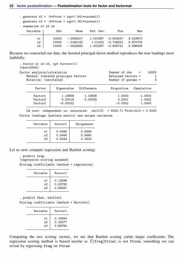
Example 11: Rescaling the scores
Let’s pretend that we work for the K. E. Watt Company, a fictional industry group that generatesstatistics on automobiles. Our “roominess” index has mean 0 and standard deviation 0.88, but indexeswe present to the public generally have mean 100 and standard deviation 10. First, we wish to rescaleour index:
. generate roomidx = (f1/.88041161)*10 + 100
. table foreign, c(mean roomidx sd roomidx freq) row format(%9.2f)
Foreign mean(roomidx) sd(roomidx) Freq.
Domestic 102.30 10.26 52.00Foreign 94.57 6.94 22.00
Total 100.00 10.00 74.00
Now when we release our results, we can write, “The K. E. Watt index of roominess shows thatdomestic cars are, on average, roomier, with an index of 102 versus only 95 for foreign cars.”
Now let’s find the “roomiest” car in our data:
. sort roomidx
. list fullname roomidx in l
fullname roomidx
74. Merc. Marquis 116.7469
We can also write, “K. E. Watt finds that the Mercury Marquis is the roomiest automobile amongthose surveyed, with a roominess index of 117 versus an average of 100.”
Technical notepredict provides two methods of scoring: the default regression scoring, which we have used
above, and the optional Bartlett method. An artificial example will best illustrate the use and meaningof the methods. We begin by creating a known-to-be-correct factor model in which the true loadingsare 0.4, 0.6, and 0.8. The variances of the unique factors are 1− 0.42 = 0.84, 1− 0.62 = 0.64, and1− 0.82 = 0.36, respectively. We make the sample size large enough so that random fluctuations arenot important.
. drop _all
. set seed 12345
. set obs 10000obs was 0, now 10000
. generate ftrue = rnormal()
. generate x1 = .4*ftrue + sqrt(.84)*rnormal()
22 factor postestimation — Postestimation tools for factor and factormat
. generate x2 = .6*ftrue + sqrt(.64)*rnormal()
. generate x3 = .8*ftrue + sqrt(.36)*rnormal()
. summarize x1 x2 x3
Variable Obs Mean Std. Dev. Min Max
x1 10000 -.0084217 1.001887 -3.804037 4.023879x2 10000 -.0190142 1.01522 -3.749022 3.870705x3 10000 -.0024562 1.002287 -3.606741 3.596839
Because we concocted our data, the iterated principal-factor method reproduces the true loadings mostfaithfully:
. factor x1 x2 x3, ipf factors(1)(obs=10000)
Factor analysis/correlation Number of obs = 10000Method: iterated principal factors Retained factors = 1Rotation: (unrotated) Number of params = 3
Factor Eigenvalue Difference Proportion Cumulative
Factor1 1.19856 1.19838 1.0000 1.0000Factor2 0.00018 0.00039 0.0001 1.0002Factor3 -0.00022 . -0.0002 1.0000
LR test: independent vs. saturated: chi2(3) = 4029.71 Prob>chi2 = 0.0000
Factor loadings (pattern matrix) and unique variances
Variable Factor1 Uniqueness
x1 0.4066 0.8346x2 0.5946 0.6465x3 0.8244 0.3203
Let us now compare regression and Bartlett scoring:. predict freg(regression scoring assumed)
Scoring coefficients (method = regression)
Variable Factor1
x1 0.12596x2 0.23782x3 0.66561
. predict fbar, bartlett
Scoring coefficients (method = Bartlett)
Variable Factor1
x1 0.16994x2 0.32077x3 0.89780
Comparing the two scoring vectors, we see that Bartlett scoring yields larger coefficients. Theregression scoring method is biased insofar as E(freg|ftrue) is not ftrue, something we canreveal by regressing freg on ftrue:

factor postestimation — Postestimation tools for factor and factormat 23
. regress freg ftrue
Source SS df MS Number of obs = 10000F( 1, 9998) =26520.45
Model 5383.48877 1 5383.48877 Prob > F = 0.0000Residual 2029.53279 9998 .202993878 R-squared = 0.7262
Adj R-squared = 0.7262Total 7413.02156 9999 .741376294 Root MSE = .45055
freg Coef. Std. Err. t P>|t| [95% Conf. Interval]
ftrue .7309397 .0044884 162.85 0.000 .7221415 .7397379_cons .0047007 .0045056 1.04 0.297 -.0041312 .0135325
Note the coefficient on ftrue of 0.731 < 1. The Bartlett scoring method, on the other hand, isunbiased:
. regress fbar ftrue
Source SS df MS Number of obs = 10000F( 1, 9998) =26520.50
Model 9794.59885 1 9794.59885 Prob > F = 0.0000Residual 3692.47929 9998 .369321793 R-squared = 0.7262
Adj R-squared = 0.7262Total 13487.0781 9999 1.3488427 Root MSE = .60772
fbar Coef. Std. Err. t P>|t| [95% Conf. Interval]
ftrue .9859229 .0060541 162.85 0.000 .9740556 .9977903_cons .0063405 .0060773 1.04 0.297 -.0055723 .0182532
The zero bias of the Bartlett method comes at the costs of less accuracy, for example, in terms ofthe mean squared error.
. generate dbar = (fbar - ftrue)^2
. generate dreg = (freg - ftrue)^2
. summarize ftrue fbar freg dbar dreg
Variable Obs Mean Std. Dev. Min Max
ftrue 10000 -.006431 1.003858 -4.200537 3.712311fbar 10000 1.00e-10 1.161397 -4.310825 4.389511freg 10000 -7.55e-11 .8610321 -3.195944 3.254285dbar 10000 .369489 .5175269 3.58e-09 4.625371dreg 10000 .2759404 .387082 4.62e-11 4.098495
Neither estimator follows the assumption that the scaled factor has unit variance. The regressionestimator has a variance less than 1, and the Bartlett estimator has a variance greater than 1.
The difference between the two scoring methods is not as important as it might seem because thebias in the regression method is only a matter of scaling and shifting.
. correlate freg fbar ftrue(obs=10000)
freg fbar ftrue
freg 1.0000fbar 1.0000 1.0000
ftrue 0.8522 0.8522 1.0000
24 factor postestimation — Postestimation tools for factor and factormat
Therefore, the choice of which scoring method we apply is largely immaterial.
Stored resultsLet p be the number of variables and f , the number of factors.
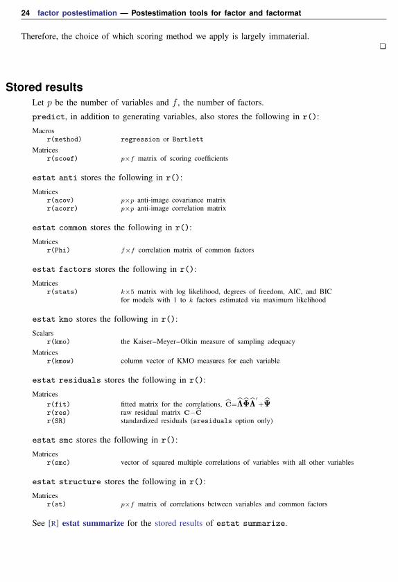
predict, in addition to generating variables, also stores the following in r():
Macrosr(method) regression or Bartlett
Matricesr(scoef) p×f matrix of scoring coefficients
estat anti stores the following in r():
Matricesr(acov) p×p anti-image covariance matrixr(acorr) p×p anti-image correlation matrix
estat common stores the following in r():
Matricesr(Phi) f×f correlation matrix of common factors
estat factors stores the following in r():
Matricesr(stats) k×5 matrix with log likelihood, degrees of freedom, AIC, and BIC
for models with 1 to k factors estimated via maximum likelihood
estat kmo stores the following in r():
Scalarsr(kmo) the Kaiser–Meyer–Olkin measure of sampling adequacy
Matricesr(kmow) column vector of KMO measures for each variable
estat residuals stores the following in r():
Matricesr(fit) fitted matrix for the correlations, C=ΛΦΛ
′+Ψ
r(res) raw residual matrix C−Cr(SR) standardized residuals (sresiduals option only)
estat smc stores the following in r():
Matricesr(smc) vector of squared multiple correlations of variables with all other variables
estat structure stores the following in r():
Matricesr(st) p×f matrix of correlations between variables and common factors
See [R] estat summarize for the stored results of estat summarize.
factor postestimation — Postestimation tools for factor and factormat 25
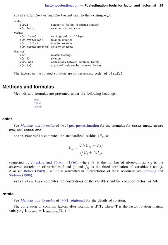
rotate after factor and factormat add to the existing e():
Scalarse(r f) number of factors in rotated solutione(r fmin) rotation criterion value
Macrose(r class) orthogonal or obliquee(r criterion) rotation criterione(r ctitle) title for rotatione(r normalization) kaiser or none
Matricese(r L) rotated loadingse(r T) rotatione(r Phi) correlations between common factorse(r Ev) explained variance by common factors
The factors in the rotated solution are in decreasing order of e(r Ev).
Methods and formulasMethods and formulas are presented under the following headings:
estatrotatepredict
estat
See Methods and formulas of [MV] pca postestimation for the formulas for estat anti, estatkmo, and estat smc.
estat residuals computes the standardized residuals rij as
rij =
√N(rij − fij)√f2ij + fiifjj
suggested by Joreskog and Sorbom (1986), where N is the number of observations, rij is theobserved correlation of variables i and j, and fij is the fitted correlation of variables i and j.Also see Bollen (1989). Caution is warranted in interpretation of these residuals; see Joreskog andSorbom (1988).
estat structure computes the correlations of the variables and the common factors as ΛΦ.
rotateSee Methods and formulas of [MV] rotatemat for the details of rotation.
The correlation of common factors after rotation is T′T, where T is the factor rotation matrix,satisfying Lrotated = Lunrotated(T
′)−1

26 factor postestimation — Postestimation tools for factor and factormat
predict
The formula for regression scoring (Thomson 1951) in the orthogonal case is
f = Λ′Σ−1x
where Λ is the unrotated or orthogonally rotated loading matrix. For oblique rotation, the regressionscoring is defined as
f = ΦΛ′Σ−1x
where Φ is the correlation matrix of the common factors.
The formula for Bartlett scoring (Bartlett 1937, 1938) is
Γ−1Λ′Ψ−1x
whereΓ = Λ′Ψ−1Λ
See Harman (1976) and Lawley and Maxwell (1971).
ReferencesAkaike, H. 1987. Factor analysis and AIC. Psychometrika 52: 317–332.
Bartlett, M. S. 1937. The statistical conception of mental factors. British Journal of Psychology 28: 97–104.
. 1938. Methods of estimating mental factors. Nature, London 141: 609–610.
Bollen, K. A. 1989. Structural Equations with Latent Variables. New York: Wiley.
Cattell, R. B. 1966. The scree test for the number of factors. Multivariate Behavioral Research 1: 245–276.
Harman, H. H. 1976. Modern Factor Analysis. 3rd ed. Chicago: University of Chicago Press.
Horst, P. 1965. Factor Analysis of Data Matrices. New York: Holt, Rinehart & Winston.
Joreskog, K. G., and D. Sorbom. 1986. Lisrel VI: Analysis of linear structural relationships by the method ofmaximum likelihood. Mooresville, IN: Scientific Software.
. 1988. PRELIS: A program for multivariate data screening and data summarization. A preprocessor for LISREL.2nd ed. Mooresville, IN: Scientific Software.
Kaiser, H. F. 1958. The varimax criterion for analytic rotation in factor analysis. Psychometrika 23: 187–200.
. 1974. An index of factor simplicity. Psychometrika 39: 31–36.
Lawley, D. N., and A. E. Maxwell. 1971. Factor Analysis as a Statistical Method. 2nd ed. London: Butterworths.
Schwarz, G. 1978. Estimating the dimension of a model. Annals of Statistics 6: 461–464.
Tarlov, A. R., J. E. Ware, Jr., S. Greenfield, E. C. Nelson, E. Perrin, and M. Zubkoff. 1989. The medical outcomesstudy. An application of methods for monitoring the results of medical care. Journal of the American MedicalAssociation 262: 925–930.
Thomson, G. H. 1951. The Factorial Analysis of Human Ability. London: University of London Press.
Also see References in [MV] factor.
Also see[MV] factor — Factor analysis
[MV] rotate — Orthogonal and oblique rotations after factor and pca
[MV] scoreplot — Score and loading plots
[MV] screeplot — Scree plot