Embed Size (px)
Citation preview
\ .
. . •
o ..
The Analysis of Lateney Data Using ~he o •
~nverse Gaussian Distribution
© Peter J. Pashley
Department of Psycho1ogy
MeG!ll University, Montréal
•
January 1987
-- \
A thesl$ submitted to the Faeulty of Graduate Studies and
Researeh in partial fulfillment of. the requirements for
the degree of Doctor of Philosophy in Psyehology
..
o .,
Permission has been granted to the National Library of Canada to microfilm this thesis and to lend or sell copies of the film.
The author (copyright owner) has reserved other publication rights, and neither the thesis nor extensi ve extracts from i t may be printed or otherwise reproduced withQut his/her written permission.
ISBN
\
1 "
L'autorisation a été accordée à la Bibliothèque nationale du Canada de microfilmer cette thèse et de· prêter ou de vendre des exemplaires._du film.
L'auteur (titulaire du droit d'auteur) se réserve les autres droits de publication: ni la thèse ni de longs extraits de celle-ci ne doivent être imprimés ou autrement reproduits sans son autorisation écrite.
0-315-38173-6
"

, ..
.. To Katharine
\
, , , ,
-
o
~:."
" '
"
. ,
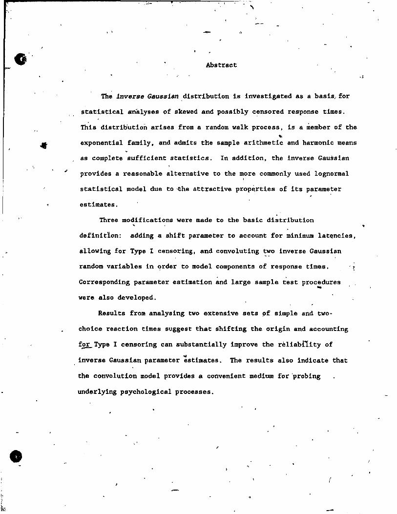
Abstract
The inverse Gsussian distribution ls investigated as a basts., for
statistical analyses of skewed and possibly c~nsored response times.
This distribution arises from a random walk process, is a member of the ~
exponential fami1y, and admits the sample arithmetic and harmonie means
, as complete sufficient statlstlcs. In addition, the inverse Gaussian
provides a reasonab1e alternative to the more commonly used lognormal 1
statistical mode1 due to ,the attractive propè,rties of its parame ter
estimates. .
Three modifications were made to the basic distribution ...
definitlon: addlng a shlft parame ter to aecount for minimum lat~ncies,
allowing for Type l censoring, and convoluting two inverse Gaussian
random variables ln order to model components of response times. , ,
Corresponding parame ter estimation and large sample test procedures .. were also deve10ped.
Results from analysing two extensive sets 9f simple and two-
choiee reaction times suggest that shifting the origin and aeeounting
f~Type l censoring can Bubstantia1ly improve the re1iabf1ity of .. inverse Gaussian parame ter estimates. The results a1so indicate that
the convolution model provides a convenient medium for'probing
underlying psycho10gica1 processes.
r
(
..
-
"
o \
o
'. ,
S olJ!Dla ire
.. La distribution provena~t de la loi Gaussienne Inverse est étudiée . '
comme une base de l~analyse statistique des tQmps dè rêponse non-
& -symétriques (en biais) et possiblement censures. Cette distribution,
,h ' , •
repartie à manière de la promenade aléatoire, est de la famille
exponentielle et reconnait les moyennes arithmétiques et harmoniques ~ .,
comme statistiques complètes et suffisantes. DG aux qualités des " ~ I.!
estimateurs des paramètres ceci présente une alternative raisonable aux
statistiques logarithmiqueSi-normales. ;"-'1 il :Trois modifications ont été portées à la définition de la
distribution de base: un paramètre de déplacement a été ajouté pour "
justifier les latences minimales. lij censure du typ~ l a été permise, .
ainsi que la circonvolution de deux variables aléatoires Gaussienn~s
inverses dans le but de tr2~ver un modèle pou~ les facteurs des temps
de résponse. Des procédures d'estimation des paramètres
correspondantes et des procédures de test pour des grAnds échantil10~s 4
'ont été deve1opées.
Les résultats de l'analyse de deux grands groupes de 60nnèes de
temps de réaction simple et de réaction à de~-choix suggèrent qu'avec
le transfert de l'origine et la justification de la censure du type 1
• on peut ameliorer cons1dérablem~nt la fiabilité des estimateurs des
paramètres Gaussiennes inverses. Les résultats indiquent également que
,le modèle de circonvolution offre un moy:en commode de sondagè du
processus psychologique.
.. .. J
..
f ,/ -, ' - 0' 'fl ' , ~ . l,
/ 'lI • , 1
1 "
o Cl;> ,
-0 Acknowledgments \~I '1 ..
",,:1
• , f
l wish to extent my,sincere thank~~and appreêiation ~,l my.the~is
\
supervisor an~mentor Dr. J. O. Ramsay, who has guided me through this
dissertation ~nd my entire doctora~ studies with great prof~CienCy, . -patience '. and at the proper times, impatience. Thanks Jim.
t Ta the other:members of my thepls committee, Dr. A. A. J. Marley
J
and Dr. D. J, Ostry, l would llke to relay my gratitude for their help
and suggestions, especia1ly during the initia!. Jltages.
l am very grateful to Dr. S. ~. Burbeck for provlding a copy of his
\ thesis and permission to use his simple reaction time samples. and to , '
r
Dr. ~.,B1oxom for forwardlng these data. l wou1d a1so like to thanK
Dr. S. W. Link for providing choice reaction time data and t~e ,
opportunity to show how llttle 1 knew about the subject when l started .
. Kuch of my. in~tial insight into the inverse Gaussian distribution" "
resulted from discussions with other researchers ~n this field,
, including Dr. G. A. Whi tmore and Dr.. V. Seshadri. l would a1so like to "
thank Dr. W. K. Petrusfc ~or his many suggestions made during our
business lunches.
Kany others asslsted with the proofreading and with the
• 1 entite thesis and was an enormous he1p in finalizing it.
Charlie. 1 Flnally, 1 would like to thank Katharine Pashley for proofreadl~g,
< • . "
tranalating the abstrac~, verifying results, helping to produc~ the J ---
• • 'li
figures, and fo~ being there. ,
vi
-.. ,
l, . , \,
o
\.
• -....
Abstract
SODUDaire
.., .
,
f~:': 4 ;~~} ,(
Acknowledgments
List of Tables
List: of Figures
Chapter 1: Introduction
Latency Data
The Problem
Contents
Current Approaches to the problem
Outline of the Proposed'Approaéh
Chapter.2: The Inverse Gaussian Distribution
Origins c
Basic Properties
,Estimati~n Procedures \
Exact Tests of Hypotheses
Heuristic Tests
Recip~ôca1 of an Inverse Ga~ssian Varlate, "
Chapter 3: Reaction Times
1
Basic Issues
Sample Data .
Random Walk Mode1s -Hazard Functions
Convolutions . ~
"-
Chapter 4: Thë Shifted Inverse Gau8s1an·Distributlon , \
vU
"- .
. . . J
,1v
v
vi
lx
xi
1
5 • 9
14
17
18
26
29
31
34
40
53
ss
60 ,1.
" ,
o
o
....
, 1
<>
Shifting the Origin 62
Estimating Shifted inverse Gaussian Parameters 69
Shifted and Censored Inverse Gaussian Distribution q7
~omputationa~ Proced~res ~84
Chapter 5: Convolution of Two Inverse Gaussian Distributions
Defining the Convolution
Estimating Convolution Parameters' '"
Censored Convolutions .~
Kodeling Components of Reaction Times~
Chapter 6: Confidence Intervals and Statistical Inference
Large Sample Tests
Shifted Inverse Gaussien.Procedures
Shifted and~Censored Inverse Gaussian Procedures
Convoluted Inverse Gaussian Procedures
Chapter 7: Discussion , '
Inverse Gaussian Vers~s Logriormal.Di~tributrons
Kodifying the Inverse Gaussian Distrinutlon
Computational Methods
Conclusions
References, . ,
Appendix A: Stem-end-Leaf Plots of Burbeck's (1979)' Simple Reaction Time Date.
" Append:Î.x B: Stem-and-Leaf Plots of LinJc' s {197'7) , Tvo-Choice Reaction rime Data
Appendix C: FORtRAN Subroutines o \
Statement of Origlnalit~ , .
J •
"
yviii
\,
88
91
94 -
96
102
105 '
108
110
112
115
117
118
, 121
133
162
188
213
',-
o , ,
'.
--
•
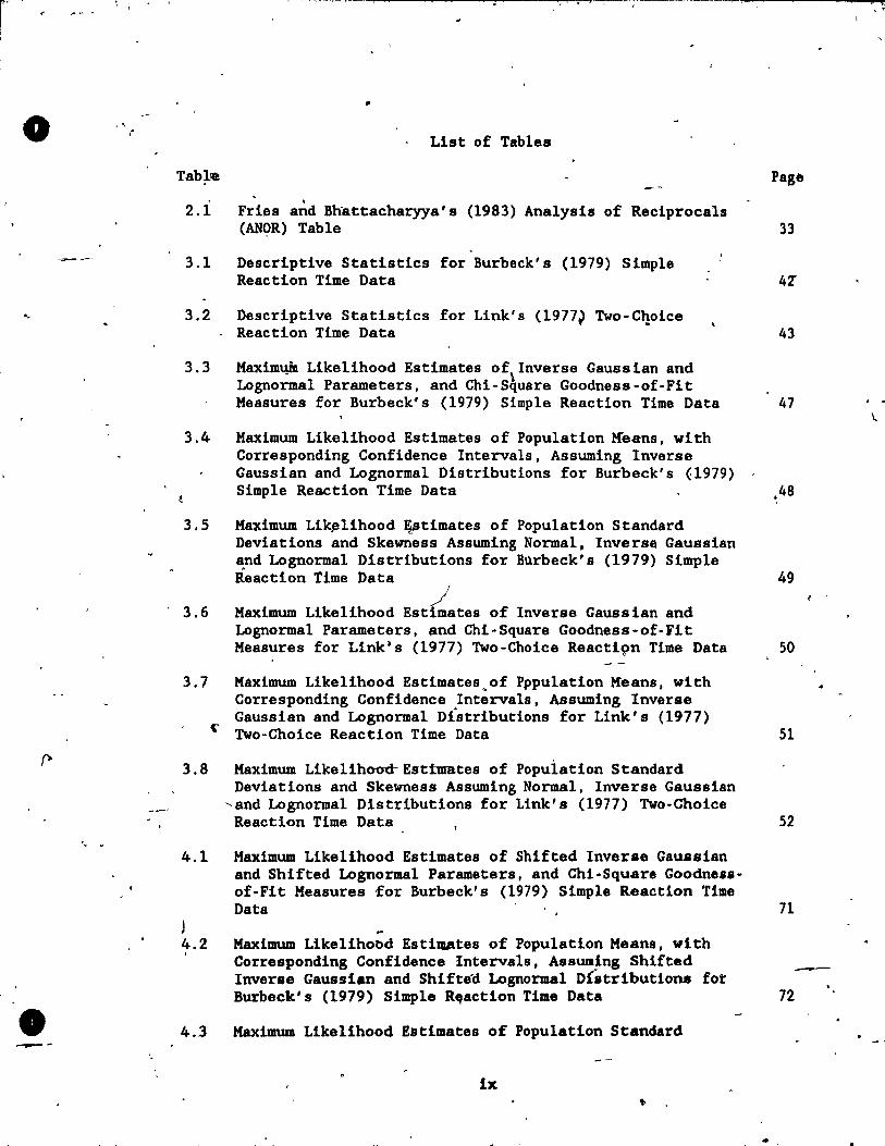
List of Tables
Table Page
2.1 Fries a~d Bhattacharyya's (1983) Analysis of Reciprocals (AN9R) Table 33
3.1 Descriptive Statistics for Burbeck's (1979) Simple Reaction Time Data 4T
3.2 Descriptive Statistics for Link's (1977~ Two-C~oice Reaction Time Data
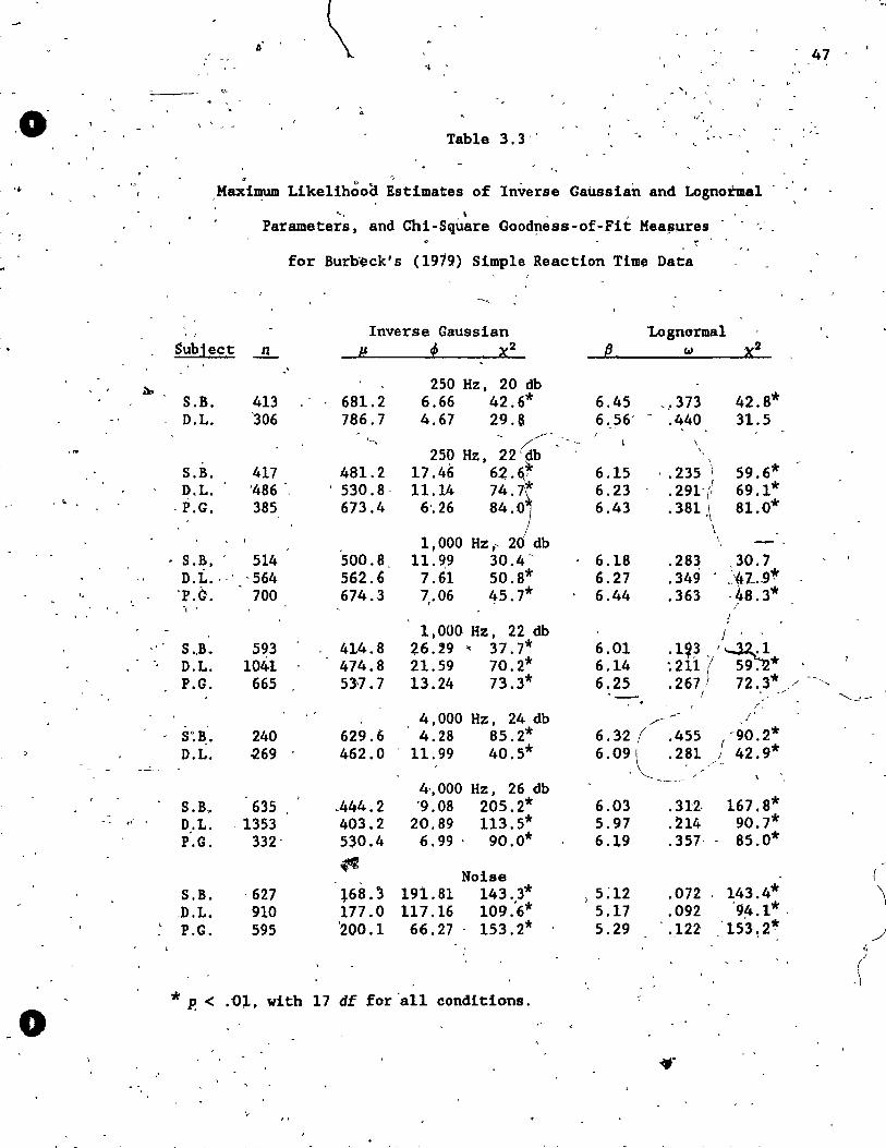
3.3 Maxim4M Likelihood Estimates of,Inverse Gaussian and Lognormal Parameters, and Chi-Square Goodness-of-Fit Measures for Burbeck's (1979) Simple Reaction Time Data
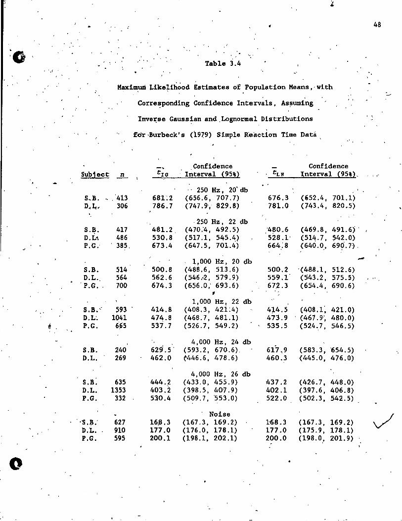
3.4 Maximum Likelihood Estimates of Population Keans, with Corresponding Confidence Intervals, Assuming Inverse Gaussian and Lognormal Distributions for Burbeck's (1979)
43
47
Simple Reaction Time Data ,48
3.5 Maximum Li~lihood ~timates of Population Standard Deviations and Skewness Assuming Normal, Inverse Gaussian and Lognormal Distributions for Burbeck's (1979) Simple Reaction Time Data 49
3.6 /
Maximum Like1ihood Estimates of Inverse Gaussian and Lognormal Parameters, and Chi-Square Goodness-of-Fit Measures for Link's (1977) Two-Choice Reacti9n Time Data 50
3.7 Maximum Likelihood Estimates.of Pppulation Keans, with Corresponding Confidence Intervals, Assuming Inverse Gaussian and Lognormal Dlstributions for Link's (1977)
~ Two-Choice Reaction Time Data 51
3.8 Maximum Likelihood-EsttmBtes of Popuiation Standard Deviations and Skewness Assuming Normal, Inverse Gaussian
~and Lognorma1 Distributions for Link's (1977) Two-Choice Reaction Time Data
4.1 Maximum Likelihood Estimates of Shifted Inverse Gau8sian and Shifted Lognorma1 Parameters, and Chi-Square Goodne.sof-Fit Measures for Burbeck' s (1979) Simple Reaction 'rime
J 4.2
Data
-Maximum Likelihood Esti~tes of Population Means, with
52
71
~ ,
Corresponding Confidence Intervals, Assuming Shifted Inverse Gaussian and Shift~d Lognorma1 Dtatributiona fot Burbeck's (1979) Simple R~action Time Data
--72
4.3 Maximum Likelihood E~timates of Population Standard
ix
..
, "
J •
:J \ .. '
o
•
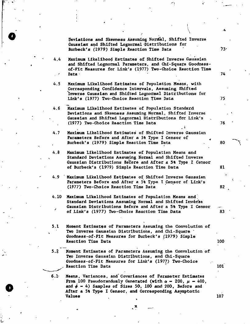
4.4
4.5
4.6
4.7
4.8
.....
( . \ Deviations and Skewness ASsuming Normal, Shifted Inverse Gaussian aqd Shifted Lognormal'Distributions for Burbeck's (1979) Simple Reaction Time Data
!Wtimum Likelihood Estimates of Shifted Inverse GauSsian and Shifted Lognormal Parameters, and Cht-Squafe Goodnessof-Fit Measures for Link's (1~77) Two-Choice Reaction Time Data'
o
Maximum Likelihood Estimates of Population Means, with Corresponding Confidence Intervals, Assuming Shifted inverse Gaussian and Shifted Lognormal Distributions for Link's (1977) Two-Choice Reaction ~ime Data
--Maximum Likelihood Estimates of Population Standard Deviations and Skewness Assuming Normal, Shifted Inverse Gaussian and Shifted Lognormal Distributions for Link's (1977) Two-Choice Reaction Time Data
Maximum Likelihood Estimates of Shifted Inverse Gaussian Parameters Before and After a 5% Type l Censor of Burbeck's (1979) Simple Reaction Time D~ta
Maximum Likelihood Estimates of Population Means and Standard Devia~ions Assuming Normal and Shifted Inverse Gaussian Distributions Be~ore and After a St Type I Censor of Burbeck's (1979) Simple Reaction Time Data
4.9 'Maximum Likelihood Estimates of Shifted Inverse Gaussian Parameters Before and Àfter a 5% Type 1 .Censor of Link! s (1977) Two-Choice Reaction Time Data
4.10
1
Maximum Likelihood Estimates of Population Means and: Standard Deviations Assuming Normal and Shifted Inv~rse Gaussian Distributions Before and After a St Type I Cens or of Link's (1977) Two-Choice Reaction Time Data
--
74
75
76
80
81
82
83
5.1 Moment Estimat~s of Parameters Assuming the Convolution of Two Inverse Gaussian Distributions, and Chi-Square' Goodness-of-Fit Measures for Burbeck's (1979) Simple Reaction Time Data . 100
5.2,
6.1-
"
Moment Estimates of Parametérs Assuming the Convolution of ~o Inverse Gaussian Distributions, and Chi-Square Goodness-of-Fit Measures for Link's (197?) Two-Choice Reaction Time Data
Means, Variances, and'Covariances of Parameter Estimates From ,100 Pseudorandomly Generated (with a - 200, ~ - 400, and; - 4) Samples of Sizes 50, 100 and 200, Before and After a St Type I Cens or , and Corresponding Asymptotic Values
101
107
-\ .
. ' .
o Figure
1.1
1.3
1.4
2.1
2.2
2.3
- 2.4
2.5
., 3.1
3.2
3.3
o 3.4
'\
..
",' r:"·"··
\.. - /
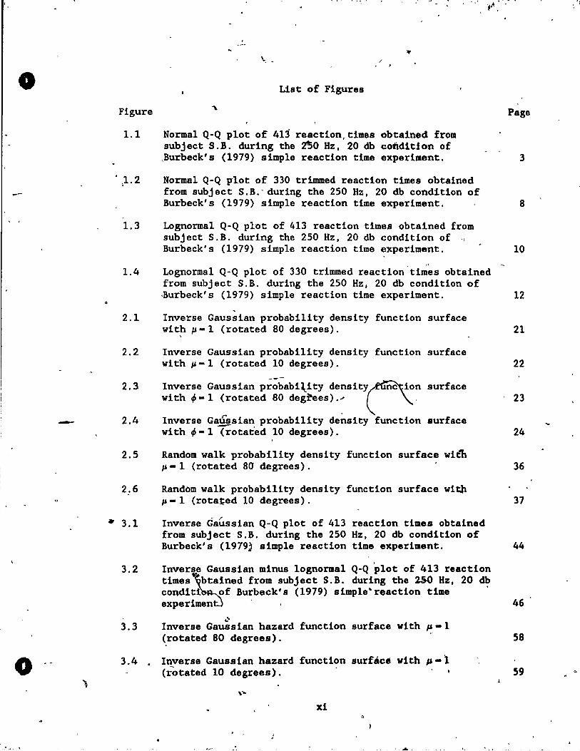
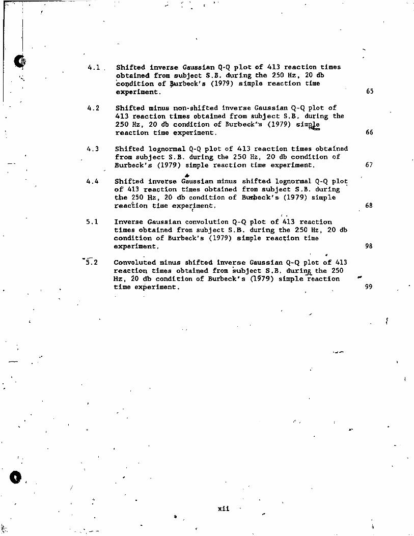
List of Figures
Normal Q*Q plot of 41j reaction,times obtained from subject S.B. during the ~O Hz, 20 db condition of ,Burbeck's (1979) simple reaction time experiment.
Normal Q*Q plot of 330 trimmed reaction times obtained from subject S.B." during the 250 Hz, 20 db condition of Burbeck's (1979) simple reaction tlme experlment.
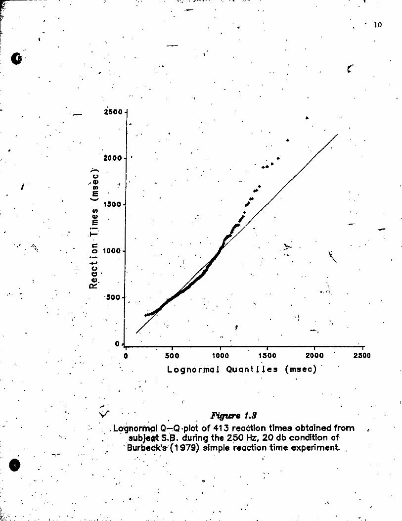
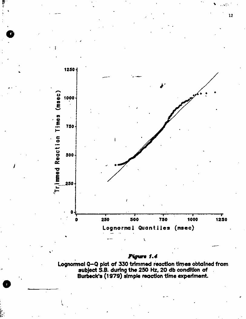
Lognorma1 Q-Q plot of 413 reaction Umes obtained from subject S.B. during the 250 Hz, 20 db condition of ., Burbeck's (1979) simple reaction time experiment.
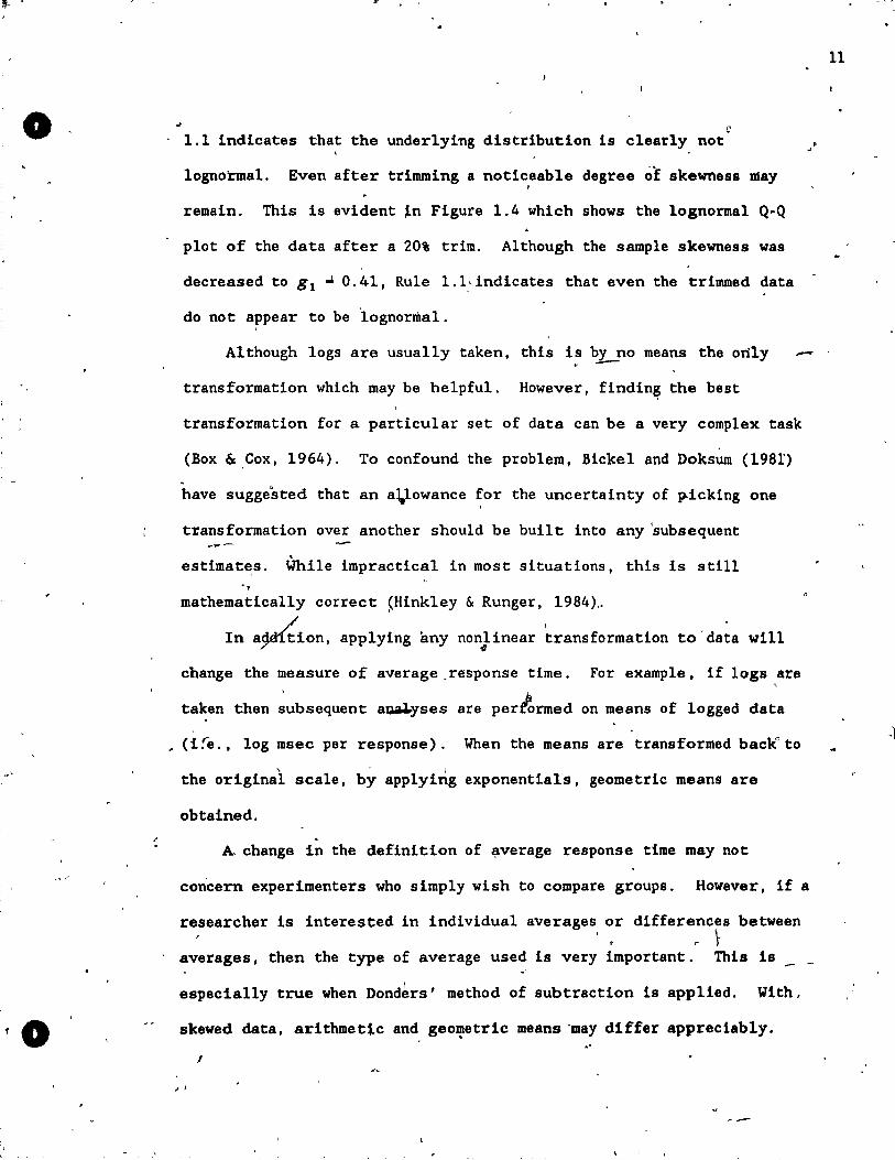
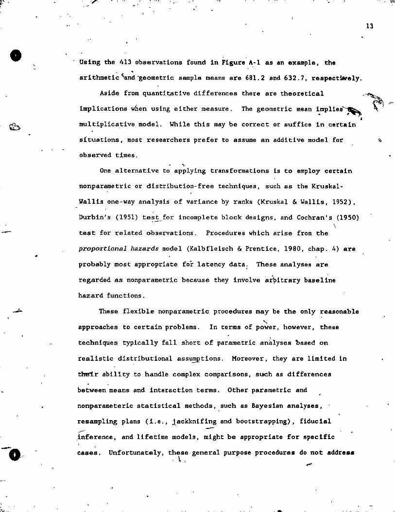
Lognormal Q-Q plot of 330 trimmed reaction'ti~~s obtained from subject S.B. during the 250 Hz, 20 db condition of cBurbeck's (1979) simple reaction Ume experiment.
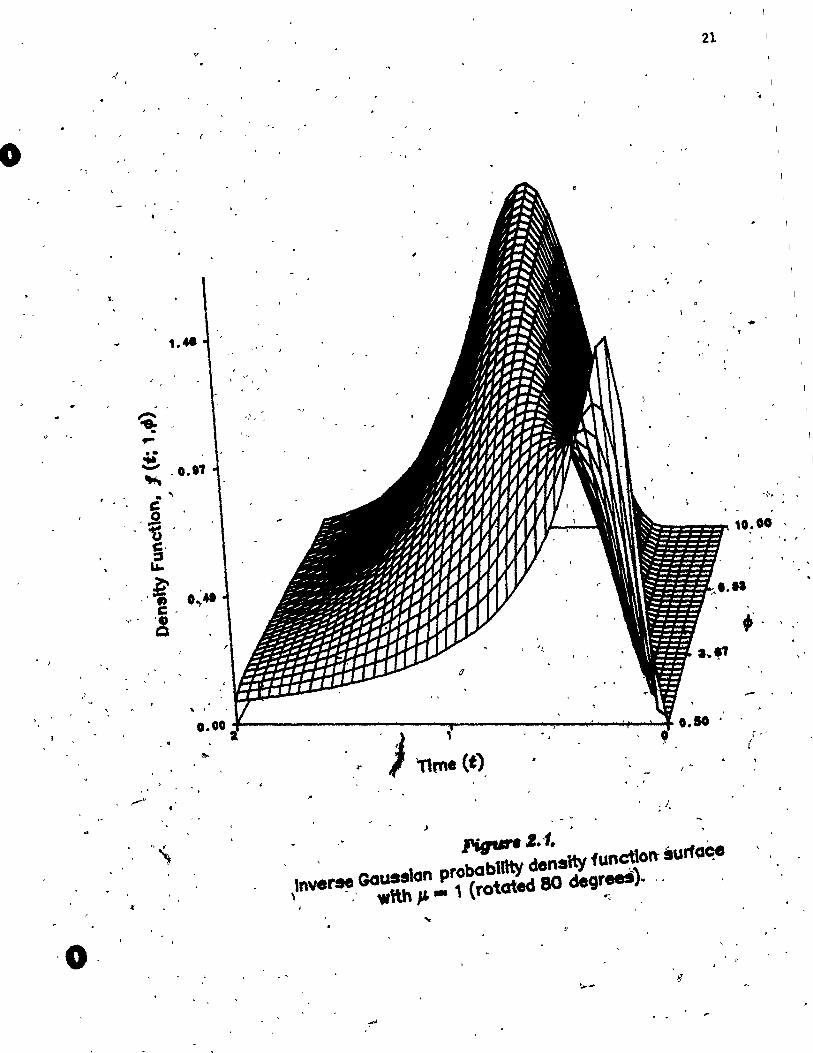
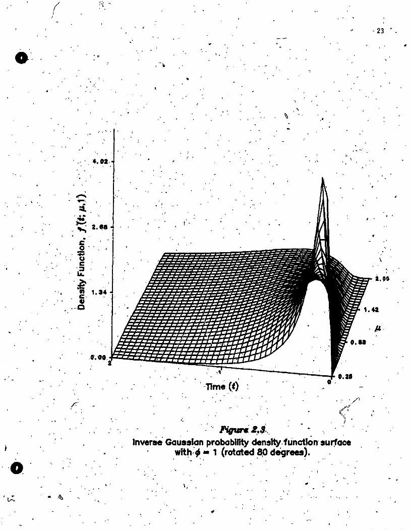
Inverse Gaussian probabi1ity density function surface wit? JJ - 1 (rotated 80 degrees).
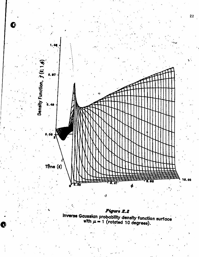
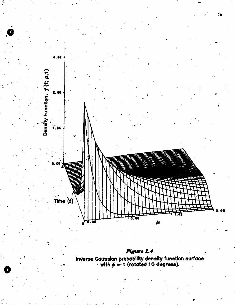
Inverse Gaussian probability density function surface with JJ -1 (rotated 10 degrees).
Inverse Gaussian p~~babi\ity density~ion surface with 4> -1 (rotated 80 deg~ees).... \. '\..'
Inverse Ga~"sian probabi1ity de~sity function surface with 4> -1 (rotated 10 degrees).
Random walk probabi1ity density function surface wit~ JJ - 1 (rotated 80 degrees).
Random walk probabi1ity density function surface with JJ - 1 (rotated 10 degrees).
Inverse Gaûssian Q-Q plot of 413 reaction times obtained from subject S.B. during the 250 Hz, 20 db condition of Burbeck's (1979} simple reaction time experiment.
Inverse Gaussian minus lognormal Q-Q plot of 413 reaction times~tained from subject S.B. during the Z50 Hz, 20 d~ condit! of Burbeck's (1979) simp1e"reaction time experimen " .
.... Inverse Gaussian hazard functlon surface with JJ-1 (rotated 80 degrees).
Inverse Gaussian hazard function surface with JJ-1 (rotated 10 degrees).
xi
' .. 6
Page
3
8
10
12
21
22
23
24
36
37
44
46
58
59
.J.-~ . '
" "
[.
, ' ".
, .
(
4.1
4.2
4.3
4.4
1
,- • " cr
, 1
Shifted inverse Gaussian Q-Q plot of 413 reaction times obtained from subject S.B. during the 250 Hz, 20 db co~dition of ~rbeck's (1979) simple reaction time experiment.
Shifted minus non-shifted inverse Gaussian Q-Q plot of 413 reaction times obtained from subject S.B. during the 250 Hz, 20 db condition of Burbeck"s (1979) simBl! reaction time expeTiment.
Shifted 1ognormal Q-Q plot of 413 reaction times obtained from subject S.B. during the 250 Hz, 20 db condition of Burbeck's (1979) simple reaction time experiment . .. Shifted inverse Gaussian minus shifted lognorma1 Q-Q plot of 413 reaction times obtained from subject S.B. during the 250 Hz, 20 db condition of But'beck' s' (1979) simple reac~ion time experiment.
(
J,
5.1 Inverse Gaussian convolution Q-Q plot of 413 reaction times obtained from subject S.B. during the 250 Hz, 20 db condition of Burbeck's (1979) simple react;ion time experiment.
,. Convoluted minus shifted inverse Gaussian Q-Q plot of 413 reaction times obtained from subject S.B. duri1!&. the 250 Hz, 20 db condi tion of Burbeck' s (19""79) simple reaction time experiment.
~ . ,
xii
65
66
67
68
98
99
"
.-1
o
Chapter-l
'. ~
Introduction
Latency Data
.... '"
\ \
Sinee the mid-nineteenth century, seientists have recognized the
potentia1 for quantifying mental events through the measurement of
reaetion times (Brebner & We1ford, 1980). As a result, reaction times
are one of the oldest and still most frequently used dependent measures ,
in psychology experiment~. Other types of 1ateney data are regu1arly
eollected through a variety of psyehology studies, inc1uding those .
invo1ving memory tasks, decision making, maze running, and prob1em
$olving. Recently, test item response lateneles havé been incorpôrated
lnto latent trait models in psychometries (e.A., B1oxom, 1985; Fischer
& lfi-s~er, 1983;. Scheib1eehner, 1985; Thissen, 1976/1977, 1983).
The focus of this thesis is on new statistica1 techniques whlch
may be used to analyse measures of.average response tlmes. Most
latency data ar~ co11ected in t1erms of units of time per re'sponse,
where the response is fixed. In these cases, a measure of average
r~sponse latency is commonly obtained by taking the arithmetic mean of .
the co1lected data. If, on the other h~nd, the number of responses ~er
unit of time is of interest. where the time ls flxed, then a comparable
measure ls achieved by calcu1ating the harmonie,mean of the observed
values (~erger. 1931).
.,J
-
o
.• ' , '
Typical distributions of response time frequencies are found in
,Appendices A and B. These are stem-and-leaf plots of data from two
-extensive reaction time experiments. The data in Appendix A, provided
through the courtesy of Dr. S. L. Burbeck, are Il,045 simple reaction
times to auditory signaIs collected from three subjects tested under
-seven experimental conditions. Appendix B contains 2,880 two-choice
re'action times from four subj ects tested under six experimental
conditions, and were made available through the courtesy of Dr. S. W.
Link. Further details of these two experimen~s are given in chapter 3.
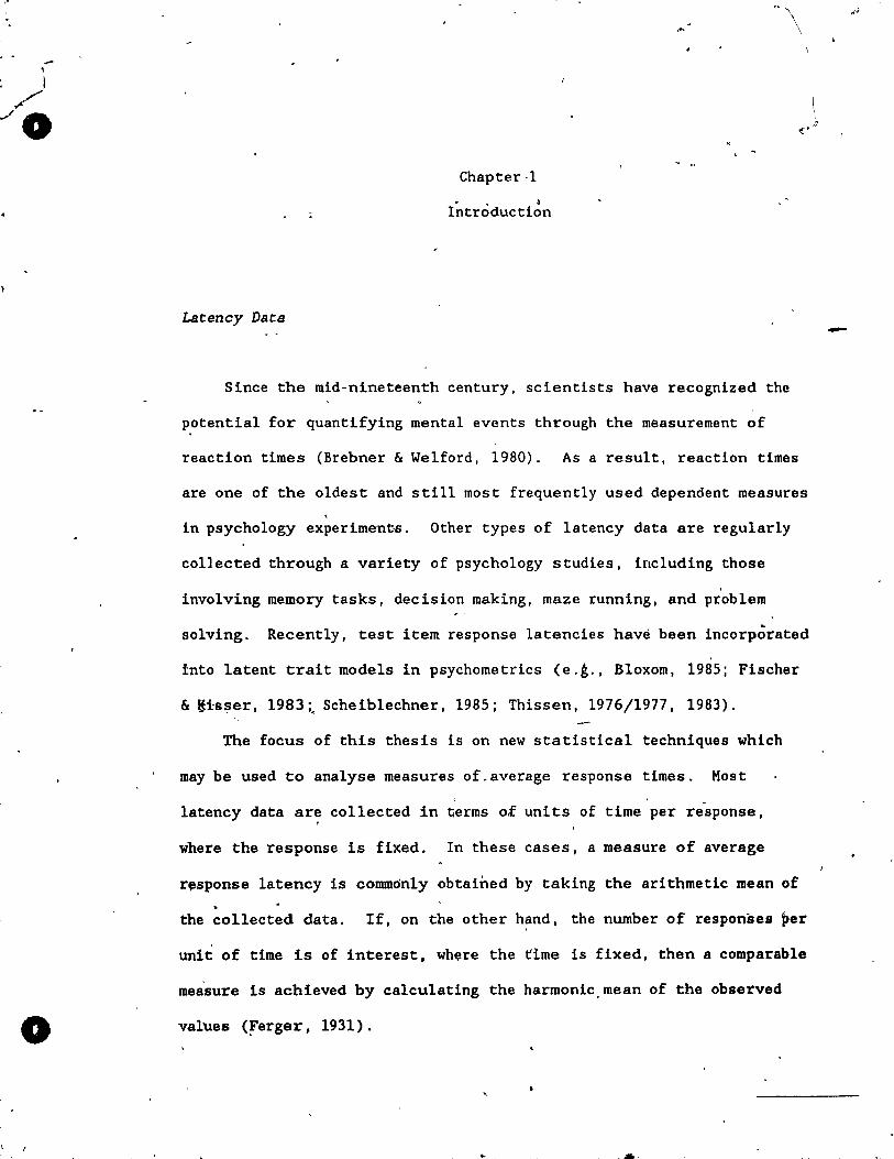
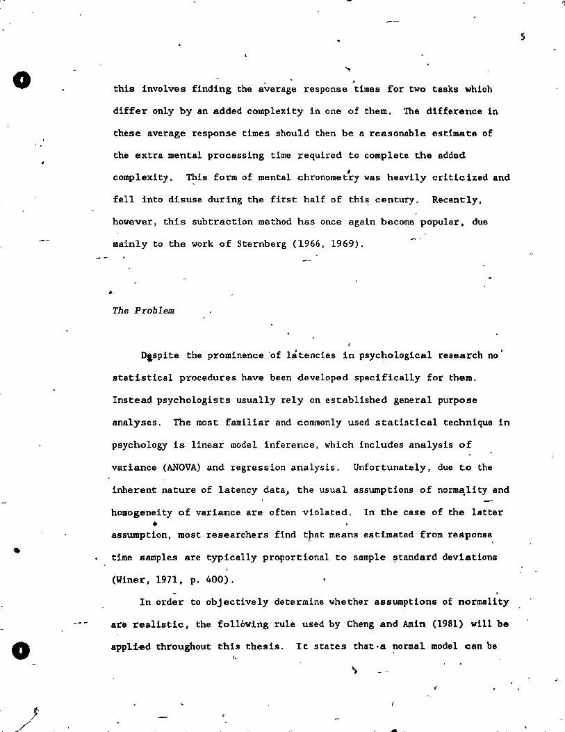
The first set of 413 observations, found in Figure A-l (Appendix
A), from subject S.B. during the 250 Hz, 20 db condition in Burbec~'s
____ ~1979) simple reaction time study, is used throughout this thesi~ as a
general illustrative example. A normal Q-Q plot èorresponding to this
set of data ls found in Figure 1.1. Here the ordered data are plotted
against the quantiles of a normal distribution with the same mean and
variance. The nonlinear trend in Figure~l.l indicates that the data
are not normally distributed. As with most latency data, these
responses possess a high degree of positive skewness. Q-Q plots •
"illustrate this trai,t weIl as they emphasize the tails of the
L distrib~tion (Wilk & Gnanadesikan, 1968).
1
Another characteristic ,of latency data is that the observed times
are always positive. In fact they are, relatively speaking, usually
conspicuously greater than zero. For i~stance, the data in Figure A-l
have a minimum value of 309 mill~seconds (msèc) while the sample mean
i8 only 681.2 msec. The absolute minimum visual and auditory reaction
times are commonly thought to be in the order of 180 msec and 140
,
"
2
.'
(' v
." '.
"\
" q.
o
.. 3
~SOO •
, \.. "
• 2000 • ,... ••
/ (,)
CD tn • E # - 1S00 tn
_CD E .-.... e o 1000 ~ 0, 0 CD
0::
500
O~ ____ ~~ ______ -r __ -' __ ~ ______ ~ ______ --'
.~OO .0 500 1000 1S00 .1 .Norma,l Quant l1es-i-msec)
\
... -. , .
Pigvn 1.1 Normal Q-Q plot 01,;,413 recrctJon tJmes obtafned from
subject S.9. durfng' the 2!50 Hz. 20 db condition of Burbeck's (1.979) simple reactlon ttme experlment.
.'
2000
"
"
~/
o
msec, respectlvely (W'oodworth & Schlosberg, 1954, chap. 2). Usua11y as
the complexity of the experimental tas~ increases so do es the
corresponding minimum reaction time.
Qulte often in practice .some individua1 trials are terminated by
an experimenter if a subject has not responded before a prespecified
timè limit. This time limit May be imposed for a variety of reasons
inc1uding equipment constraints 1 1aboratory availablity 1 and subject
fatigue considerations. This procedure ls a form of Type l censorin.g
(Ka1bf1eisch & Prentice, 1980, chap. 3; Lawless, 1982, chap. 1).
Progressive Type 1 censoring, where more than one fixèd time limit is . --used, and Type II censoring, in which a limit on the number of
responses is applied, are not considered in this thesis.
Besides ana1ysing raw 1atency data, many psychologists are
interested in certain components which contribute tow'§!,ds the total , .
1atency time. Vith regard to reaction times in particular.
investigators tiy to break the raw data down into two main parts. The
firs.t and most important is the decision 1atency, which consists of the
time required tÇ> perfc;>rm a specifie mental task. The second relates
aIl other activities needed to perform the required task and is 1'1
, common1y referred to as the residua1 1atency or motor time.
Researchers often assume that the processes associ~ted wit:h the
declaion and residual times..&Q.t in an independent additive serial
manner '(Luce, 1986, chap. 3). These convenient supp,ositions are also
assumed in this thesls.
One approach to estimating certain components of latency times is
to use F. C. Donders' (1868) classic method of suhtraction. Initially
o(
•
4
o
'.
o
" this involves finding the average response times for two tasks which
differ only by an added complexity in one of them. The difference in
these average response times shou1d then be a reasonable estimate of
the extra mental processing time :required to complete the added
comp1exity. f
This form of mental chronometry was heavlly crlticized and
fell into disuse during the first half of thi~ century. Recent1y,
however, this subtraction method has once again become popular. due
main1y to the work of Sternberg (1966, 1969).
The Problem
Dlspite the prominence 'of l~tencies in psyc~ological research no
statistical procedures have been developed specifically for them.
Instead psychologists usual1y rely on establlshed genersl purpose
analyses. The most familiar and commonly used statistical technique in
psychology is linear model inference, which includes analysis of
variance (ANOVA) and regression analysis. Unfortunately, due to the
Inherent nature of 1atency data) the usua1 assumptions of norm~l1ty and
homogeneity of variance are often vio1ated. In the case of the latter
• assumption, Most researchers find that means estimated from response
"
tlme samples are typically proportiona1 to sample ~tandard deviations
(Winer, 1971, p. 400).
In order to objective1y determine whether assumptions of normal1ty
are realistic, the follôwing ru1e used by Cheng and A{nin (1981) will be
applled throughout this thesis. It states that·a normal model can be
(
5
, ' ,',
,
o used if the samp1é skewness, denoted by (j&tisfie.
gl < k(6/n)%' (1.1)
"where n Is the sample size, and k is a positive constant ~ndlcating the
1evei of confidence. This rule follows from the fact that .gl is
asymptotical1y' no~al with mean 0 and varfance 6/n when the underlying
distribution is nearly normal (Kendall & Stuart, 1977, chap. 10). In
the case of the data shown in Figure A-l, since the sample skewness
(gl - 2.14) 18 greater than k'(6/n)% - 0.28, where k - 2.33, the"
probab;~ity that the u~derlying d~stribution is nearly normàl is much
less than 1%. Note that through~ut this thesis the measure of skewness
ls calcplated as 81 - ml /s3
,.. ,,(here ml ~is the t~~rd moment about' th~
mean and s ls the s~p~e standard deviation.
The rule,given,in Equation 1.1 ~nly indicates when assumptions of
normality are suspect .. It cannot determine,whether procedures, such as-. '
ANOVA, c~n be used legitimately to analyse "a particular set of data. . ,
. However, an investigator will have.more 'confidence in meeting specified " "
test signlficance and power levels' if real1stic distributiona1
assumptions are made. While Many commonly used statistical tests'of ,
si~lficance are quite robust 'wlth ~egard ta slight departures from the .. -' assumptions of normality and hORlogeneity of variance (Box, 1953),
, 1 _ ~
recent studles have indicated Chat erroneous conclusions may be drawn
from applying these methods to very skew~d data (Bradley, 1~80a, 1980b,
J980c, 1984; 'Glass, Peckham, Sr Sanders, 1972; Wike & Chur ch , 1982).
, As violations to assumptions of normality for latency 4ata
t ••
. ,
6
,

o
'.
, .
o
"
~.
generally result from taU attributes of the distribution,_ outlièrs'
might. be suspected of cau'dng the problem .. Measures of central
tendency which are not ovedy sensitive to outliers., ~uch as medians,
may be, used for these cases. Unfortunately, investigators who apply
these 'à.lternat:iWe statistics are subsequently severély restricted in
tenns of the availability of corresponding hypothes1s testing
procedures. ,"'\
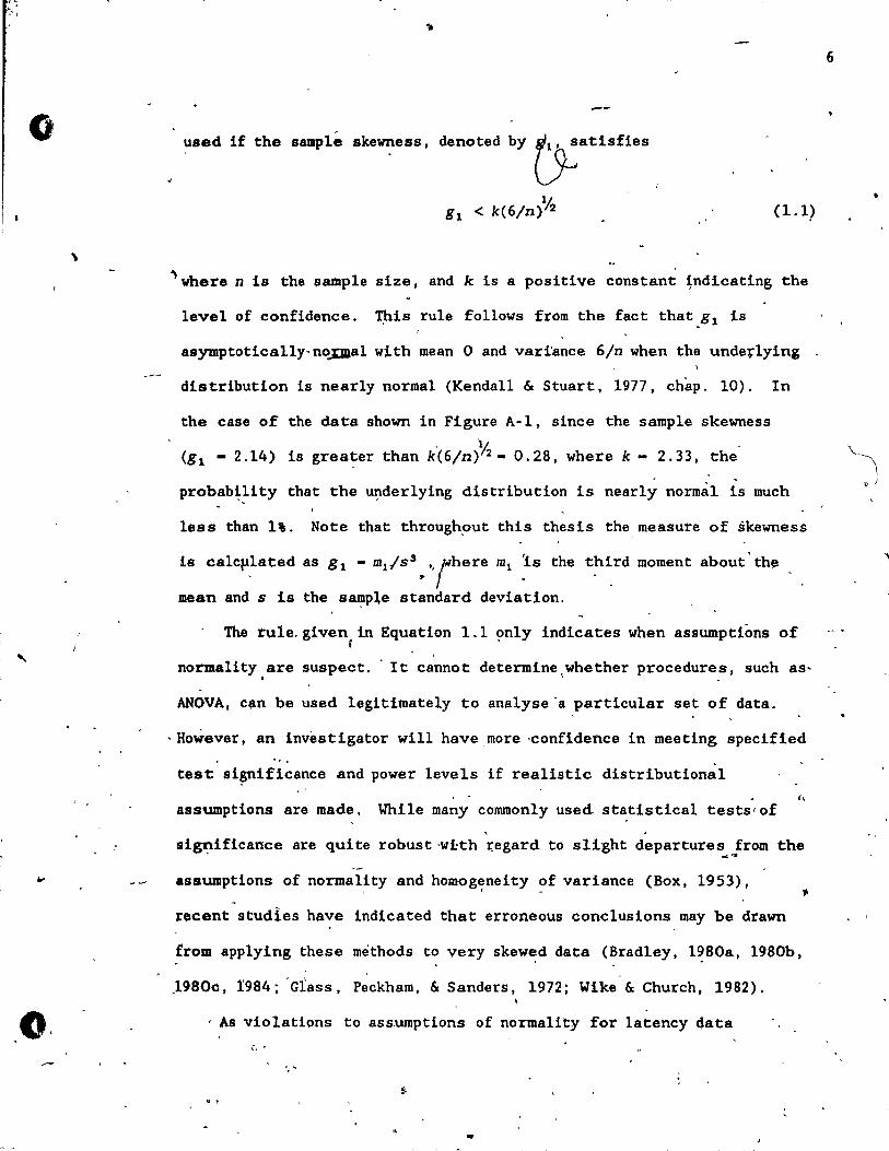
Tecfiniques such as winsorizing ,and trimming are also available to
<-dea1, wi-th out1iers, however. their effect on most 1atency data is not
. worth the subsèquent 10ss in information. For instance, consider
Figure -1. 2 w~ich contains a normal Q-Q plot" of, the data after 10% of
Though there is sorne
impr~vement, de-finite deviations from normality remain, ln fact, the
f\ '-A sampl~ gl - 0.84 was found to be gr~ater than k(6/n) 2 -0.31, where
k - 2.33 and n - 330. So by Rule 1.1, even the trimmed data do not
appear t9 be normal . .
Besides, the assurnptions of normality and hOJ1logeneity o'f variance,
'.'. the simplicity of ~odels and additiv.ity of effects in compl~x designs
~
sh-ould also be considered. In mixed models an increase in variance
tlssoC1ated with the main effects can result from an interaction between . t , (
random and fixed factors (Winer, 1971.., p. 398). Also, 'certain designs
in which interactio~ effects are totally confounded w{~h experimental
error require strictly additive models. The use of more reaUstlc
distributi~n assumptions may result in simpler mod~l; and thu~ ",
alleviate som~ Qf these difficulties. , " In addition to problems with undérlylng assÙlDptions, cOlDIIIon
7
•
o
.'
"
,'0-
, , ~ ,
'1250 "
""' ~ 1000 ., e .,
,ID ~ E ',' .- 150 1- ' -
·C
\
..
. 1 ,0
!
. . -..., u g 500 tD
a:::
. - "
, .
"
O~ ______ ~ ______ T-__ - __ ' __ ~ ______ ~ __ ~ __ ~
. ' . ,,'
o , '
_ 250 . 500 750 1000 J, 1250
Normal tJùantlJès' (ms~c)
, , \ -, '
, . JYvre,'.~-, Normal Q-Q plot 01 330 trimmed reactlon tlmes obtalned from ' . " subject S.8. during the 250 Hz ... 20 db conclltlon of '
Burbeck'~ (1979) simple reQctlon t1rr-e ~periment. ~ .
, o ,
,.
8
\
0,
•
, ., hypothesis testi~g theory does not handle censored dat~ weIl. In
practiae many psychologist~ simply throw out censored point~. This ls
a wasteful and potentially biased approach. Though th~y do not
indicate precise1y when a sûbject responds, censored times do provide.
information' about the taUs of the ut:'derlying- dis,tribution. Through
.dre proper use of censored inform~tiori 'invest~gators can increase the ,
precisio~ of their populat40n param~t~r estima~es.
" l '
C~rrenl: Approaches, ,1:0 the Problem
. In order to use familiar hypothesis testing methods, psycpologists - .,
typically modify colle~ted latency data so th~t the usual underiyin~ .. .... , • J
assumptions of normality and homogeneity of'variance are approximately
satisfied. ..... The most commo~ly us~d procedure i~ ~o rescale the Qata by
apPlying logarithmic transformations. This is equival~nt to assuming a
lognormal model. In Most caser'log transformed' latency data are more
nearly normally distributed and the heteroscedastici~y prob1em is'
improved',
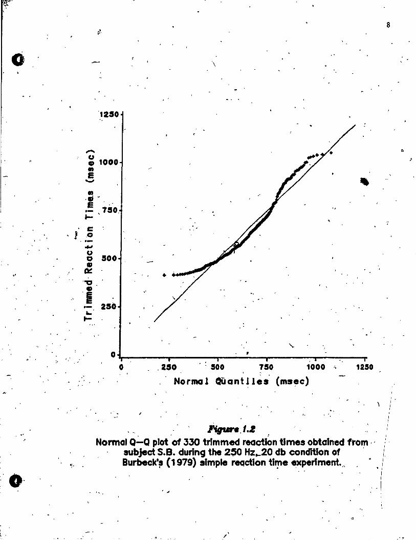
'(l- , ' . Unfortunate1y. a noticeab1e amount of skewness êan remain after
, . applying log transformations. For instance, consid~r the'lognormal Q~Q
, , ~
plot in Figure 1.3 of the data given !n~~igure A-I from subject S.B. . , ~ ..
~ 1
in Burbeck's simple reaction time exper1ment: Though an ~mprove~ent ls J.
evident a substantial amount of skewness ls not ac~ounted for by th~ -"or , • ~
log transform~tion. The samp1e skewness of the logged' data ia equa1 to , "
: 78,' which 18 still quite high . ,-
.. <>,
,,/ 1 .. ••
..... ' .',
• . .
9
, '
'.
.'
0-
" À , - ~~
'.
" • ~
~~~~: .~
- .'
....• J
/
'-
• !
--
, ,
.'
-,-
."' ...... .- ,
- 10
,
;-.. (.)
)lI CI) 0)
e ""'-J
0)
CI) E .-
-1-'
c 0 .-....., (.)
C' CI).
0=:
, ,
, 2500
2000 •
-1
1500
1000
'500 " ' '
, 1
., "
• • •••
•
, )'o.,
•
, 1
- .
(
'01 ~i--------~------~--------~,~------~------~ o 500 1000 1500 2000 2500
L 09 no r ma 1 Qu an t Ile s (mse c) .
," ~'
v , Pig1J:re t.9 :, '.' L~or~1 Q~,Q oplot of 413 reaètton tlmes obtolned from
. ' ,subJett S.e. during the 2;50 Hz, 20 db condition of: ." , Burbeck's-" (1 979) simple reactlon time experiment. , . ,
.' .
, 1
,-.. .. .. '
, . _i . •. _
--
o 11
a 1.1 indicates that the under1ying distribution is c1ear1y not
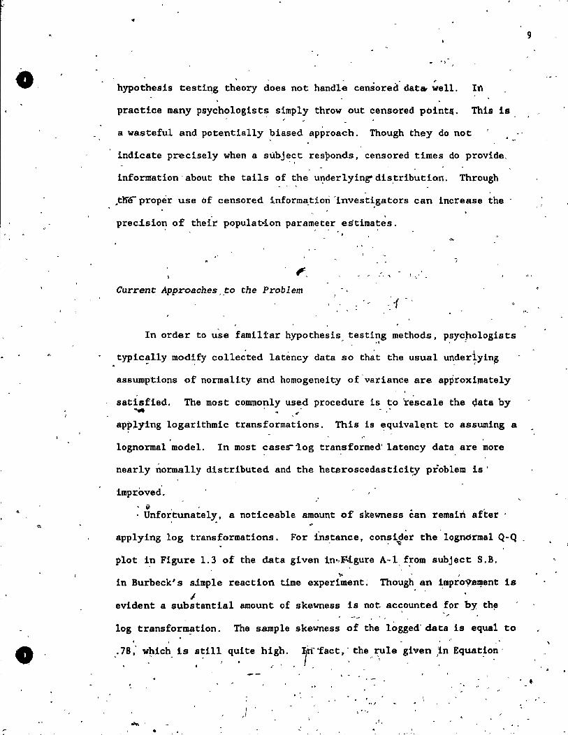
lognormal. Even after trimming a noticeable degree of skewness may
remain. This is evident Jn Figure 1.4 which shows the lognormal Q~Q
plot of the data after a 20% trim. Although the sample skewness was
decreased to gl ~ 0.41, Rule l.l, indicates that even the trimmed data
do not appear to be lognorma1.
A1though 10gs are usua1ly taken, this is by no means the orily ,.-r-
" --transformation which may be helpful. However, findin~ the best
transformation for a particular set of data can be a very comp1ex task
(Box & ,Cox, 1964). To confound the problem, Blckel and Doksum (198r)
have suggested that an a~owance ~or the uncertainty of ~icklng one
transformation over another should be built into Any subsequent
estimates. While impractica1 in most situations, this is still "
mathematically correct ~Hinkley & Runger, 1984),.
In a~ion, applying any non}inear transformation to'data will
change the measure of average _response time. For example, if logs are ,
taken then subsequent a~yses are per~rmed on means of logged data
, (i re., log msec per response). When the means are transformed backo to
the original scale, by applyi~g exponentials, geometric means are
obtained.
A, change in the definition of ~verage response time may not
concern experimenters who simply wish to compare groups. However, if a
researcher is interested in individual averages or differences between ; 1 Il r t
averages, then the type of average used is very important. This ls
especially true when Donders' method of 9ubtraction i9 applled. lUth 1
skewed data, arlthmetlc and geo~etrlc me ans 'May dlffer appreclably. "
f
, 1
o
~
...
J
.~
1
•
, ...
, 1
125
°1 ,..... ~ 1000 CD E '-'
CD 'G
E 150 .-
t-
e 0 .-..., u 0 500 G
0::
"0' G
i ·-__ 250 ~
J-
. O~------~----~-r------~-------r------~ o 250 500 150 1000 1250
Lognormal QuantlJes (msec)
l'tgvn '.4-Logno,mal Q-Q plot of 330 tnmmed react10n tllY,l. obtalried from
subject S.B. du ring the 250 Hz. 20 db cond1tlon of Burbeck's (1979) simple reactJon ttme experlment •
12
r·
•
.. /'
13
. ,
Using the 413 observations found in Figure A; 1 as an example. the
arithmeti~ ~and 'geometric sample means are 681.2 and 632.7 , respectJNely.
Aslde from quantit.ative differences there are theoretical _-~
implications when using either measure. The geometric me.n ~mpU •• ~ ~;.. •
multiplica~ive mode1. While this May be correct or suffice in certain
s!tuations. Most researchers prefer to assume an additive model for
observed times. '.
One alternative to app1ying transformations is to emp10y certain
nonparametric or distribution-free techniques, such as the Kruska1-
Wallis one-way analysis of variance by ranks (Kruska1 & Wallis, 1952),
Durbin's (1951) test for incomplete block designs, and Cochran's (1950) .--\
test for re1ated observations. Procedures which arise from the
proportions1 hazards model (Kalbfleiseh & Prentiee, 1980. chap. 4) are
probably most appropriate for 1atency data: These analyses are
regarded as nonparametric because they involve ar~itrary base1ine
hazard functions.
These flexible nonparametric procedures May be the only reasonable .....
approaehes to certain problems. In terms of power, however. these
techniques typica1ly fal1 short of parame tric an~lyses based on
realistie distributiona! ass~tions. Moreover, they are limited in
the1r ability to handle complex comparisons, such as differences
between means and interaction terms. Other parametric and
nonparameteric statistieal methods, such as Bayesian analyses, .
resampling plans (i.e., jackknifing and bootstrapping), fiducial /'"
,inference, and lifetime models, might be app.ropriate for specifie
cases. Unfortunately, these general purpose procedures do not addre •• ~ \
-
._,.::\, ..... -- 1 -'"1 .i l - ~. - .~ .. ,;
, '. ... ,. ,
14
/
o aIl the issues which are particular to 1atency data, such as estimating , e
, decision and mQtor time parameters.
Outline of the Proposed App;~ach
..".
The objec~iye of this thesis is to deve10p statistica1 Inference " .
techniques, based on a rea1istic parametric model! which may be applieœ
to the arithmetic means of latency data. For the mean to be a
8ufficient statistic (i.e., no information i8 lost through summatiDn)
the model must ~e of the exponential fami1y type (Kendall & Stuart,
1973, chap. 17). Burbeck and Luce (1982) found that of the
distributions of this type proposed for reaction times, on1y the
inyerse Gaussian distribution possesses the attributes required to
model simple reaction times properly:
Contained in this thesis are new statistical techniques, based on
the inverse Gaussian distribution, which are suitable for most latency
data. The inverse ~aussian distribution h a family of unimodal
positively skewed curves which have been used recerttly to model a wide
variety of data from various scientific fields. These inc1ùde tracer ~
dilution curves in cardi610gy (W~se. 1966), noise intensities (Marcus, 'f
1975) •. labour turnover (Whitmore,' 1979), and product interpurchase
--times (Banerjee & Bhattacharyya, 1976). lts basic properties a1low it·
to be ·the-roundation for numerous statistical procedures which paralle1~
Many common tests of significance for· normal data, such as Student's t
• test and ANOVA .
•

o
--
o
.,_ ..
A review of basic inverse Gaussian distribution properUes i8
presented in chapter 2. Analogies between statt,stical tests based on
the inverse Gaussian and those for normal data arè emphasized. Also
- "tliscussed it- the rec iprocal of an inverse Gauss ian varia te, which may
'be of interest to investigators who prefer to work with criterifl
,1
measured in terms of responses per unit of time.
Although the techniques discussed in this thesis can be used with
most types of latency 'dp.ta, emphasis will be placed on their
application to reaction times. Ghapter 3 reviews reaction Ume
characteristics and theoretical models which suggest that the i~verse
Gaussian is a reasonable distribution to consider. lncluded is a
di~cussion of the inverse Gaussian' s hazard function. Also discussed
are the experimental data sets upon which procedures outlined in
chapters 4 and 5 were tested. .. While the basic inverse Gaussiàn distribution models latency data
.. skewnes!! well, its minimum value is always zero. Procedures which
improve the fit of the inverse Gaussian to reaction ti!!les by shifting
the origin will be discussed in chaptel' 4. The basic procedure for
shifting was first presented by Padgett and Wei (1979). This approach .
is expanded to handle censored points, and ~ new computationa! algorithms
for obtaining maximum likelihood shift parall!eter estimates are
outlined.
As mentioned earlier, psychologists are often ~nterested in «
components of total reaction Umes. Techniques for estimating decision
and r~sidual time parameters, by assumi.ng a. convolution of two inverse
Gaussian variables, are presented in chapter 5, as well as procedures
f.
15
,-
( \
>,
\.
(;
o
for apply1ng Donders' subtract10n meth~~.
Most estimation techniques developed in this paper are of the
maximum l1kelihood type. Large sample statistical tests which can be
based on these estimates are discussed in chapter 6. Also presented
are the results of a simulation study of the behaviour of the censored
and noncensored shifted inverse Gaussian parame ter estimates.
Throughout this thesis the results from inverse Gaussian
procedures are compared to those obtained from assuming a lognormal
model. Further discussion of the advantages and disadv4ntages of using
• e1ther ,the inverse Gaussian or lognormal distributions Is presented in ., chaptéir 7. In addition, suggestions are made for future research in
this area. ,
..
16
o
-)
o
,
Chapter 2
The Inverse Gaussian Distribution
Origlns
The inverse Gaussian distribution was first deve10ped by
Schrodinger in 1915. He presented it as the probability density
function associated with the first p,~ssage time .of Bro~ian motion with
,positive drift (or equivalently. a restricted random walk process wit~
sma11 step sizes). In other words 1 the tnverse Gaussian distribution
can be obtained by supposing that a particle' moves along a line subjeçt
to Brownian motion with positive drift Il and variance 0 2 . Then T, the
time required to travel a fixed distance d, is a randorn variable with
probability density function
d - [_ (d-lIt)2 ]. f(t:) - ;J(21ft3 ) exp, 202t • t:, Il>0. (2.1)
Wald (1947) derived a similar fami~y of distributiohs -às a ..
limiting form of the distribution of the average sample size in a
sequential p,robability ratio test. Bartle,tt (1966) genera1ized Wald' s l ,
derivation by applying Wald' s fundal\lental identity of sequential
analys'is to the first passage time in random wa1ks. ThiS'
generalization can be accompli shed by letting ZI' Z2' ...• Zn be
independent ide~tically dlstributed random variables with finite
17
O·
o
,
expeeted value E(Z) > -0 and nonzero var~anc var(Z). Also, let-the " . n
random variable N be def~ned- by EZj .é; d, n l, 2, _ o. • ., N -1 .' and H 12j ~ d, for fixed d > O. The' distribution of N/E(N) , as E(N) -+ CIO. iS
then known as the Wald distribution and is special case of '(2.1)
where dlll - 1.
Most of the current interest wlth the nverse 'Gaussian
distribution stems from the pionéering work by M '.C. K. Tweec!ie. ,He Z--,' .' , ,was the first ta tho,roughly in~e~tigat,e tpè basic chaÏ'a~te-ris~iés and
. -statistical properties of thls distribution (Tweedie, 1957a, 1957b).
Tweedie .(1947) was also the first to apply he name inverse Gàussian.'
TItis choice resulte,d from noting the invers relationship between the
cumulant generâting functions (i.e., logari hms of the Laplaèe , \
transformation of the pro'babil?ty densitles corre.sportd~ng to this' , ! .
distribution ~nd the Gaussian or normal dis ribution. {
;. ........ "-
'j
Baslc Properties -
The most common form of the inverse Gausslan probabllity density ~
function i8 obtained by substituting Il .. d/p and 0 2 - d2 /À int;o '
~quation 2.1, which yields
.
, .' . ,( À)% ~{ ~t-I')2] f(t;p,À)- 21ft' ex.p ~ 2p2 t for t, p, À> 0 J
- . . - 0, 'otherwise.
, -,
\
18
4
-'1/:-
;
o
)
'0
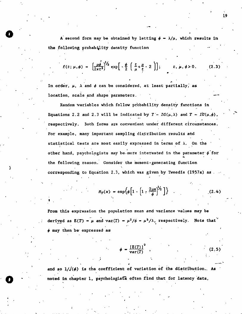
A second form may be obtained by letting ~
the !ollowing probab~lity density function
~/~. which results in
t, #l, ~> o. (2.3)
• ..
" In ordèr, ~, ~ and ~ can be considered, at least partially; as
location, scale ~nd shape parameters, ' --Random variables wh1ch follow probability den~ity functions in
Equations 2.2 and 2.3 will be indicated by T'- IG(~,~) and T - Ib(~,f), - , ,
respectively. Both forms are convenient under different circumstançes.
" For example, màny important sampl1ng dis~ribution results and G
st4tistical tests are most easi1y expre,ssed in terms of~. On the ' 'J
other hand, psycho19gists may be.more interested in the parameter'~ for
the following reason. Consider the inoment-generating function
corresponding to Equation 2.3, which was given by Tweedie (19.57a) as ,
"
HT(x) -exP{~[l- (l:~rh]} ,(2.4) ' . •
From thls expression the population mean and variance val~es may be " .
deriy!d as E(T) - p and var(T) - p2 If - ~3 /~'. respectively.
f ~ay then be' expressed as
"
f _ [E(T)]2 var(T)
Note that '"
19
'. --. and so I/J(~) is the co~fficient of vatiatlon of the dl~tribu~lon., As '
noted in chapter 1, psychologtsfi often find that for latency 'data,
"
.... .
,
0'
-" ,
1 .
means are proportional to the _,standard deviations across groups. This
translates into a constant ~ across groups-When the inverse" ~an ~;r-.
dis'tribution i8 used.
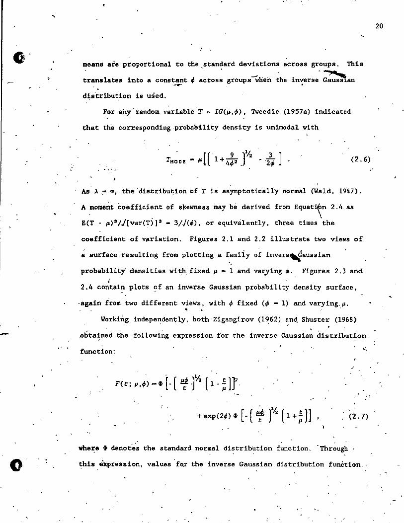
For any'random variable T - IG(~,~), Tweedie (1957a) indicated
that the corresponding.probability density is unimodal with
[( ' 9]% THOD ! - 1" 1 + 4~2 _ (2.6)
A!J ~ ,:+ CIl, the 'dis,tribu~ion of T Is asymptotlcaliy normal (Wald, 1947).
A moment éoefficient of skewness may bè derived from EqUat~n 2.4. as
E(T - ~)s/j[var(~j]S - 3/J(~), or equivàlent1y, three times the
coefficient of v~riation. Figures 2.1 and 2.2 i11ustrate two views of
~ surface resulting from p10tting a ~amiiy of invers~aussian
probabi1ity densities wi~~fixed ~ - 1 and varying~. Figures 2.3 and J
2.4 contain plots of an inverse Gaussian probability density surface, - '
·aga1n from two different views, with ~ fixed (~ - 1) and varying)J. .. Working indepe~dently, both Zigangirov (1~62) ~n4 Shuster (1968)
• ~bta~ned the fo11owi~g expression for the inverse Gaussian dist~ibution
function:
, ,
,
(2.7)
where t denot~s the standard normal distribution funct~on. 'Through
~his expression, values fo.r the inverse Gaussian distribution funètion,'
, .
, .
20
21
"
o
,'-
. -~ ~ ,O.t1
" '
l '
, i , ' , - "
)
~J.'I.
,'RYe'" GGusskln probablllty dens!ty functlon- Surf~ , .' wlth ~ - 1 (rotated 80 de9r~)· .' .
\>.-
"
•
10.00 '
.' ,
-i 1
;- ~ ,
. '
, "
• 1
.. - - ....
, 0 22
o '. '. "
I~ . ./
, " .
1. ~. . . .
, , '< ,'\:·1 ' . . . , : -.
, . . ~, ... \
G
0 ; . . , --J
.' ,
, 1
- . , "~ -\' . . ,
" ~~~ " • '1 " , ~~r-' . ,
" , ~~:I'''' .. -, .
, . , '~~r--
, .. ~~ , ~~~~-. <Jo ~~ .
A:'l l'
. .. f . .
0.0.
, .
f ~ n ~"":"" l'''r-
"
..a r- r-~ i'" -i"" i"'1"- f'" t"-I""~ ...
0 l'N N 1"'" 1'1"< i"'1"- i'" ~ f"'r-~ ~ l' " ~!'
.... .... r"'r- .... ,.. r.. .
Î' l' r'" l"'- l' l'''r- r-J ~ l' f\ 1" l' i'r' ...
r"" f'" f\ t'r.. r-- r-r-1\ ~ f\ i\ r"- f'1"' r l'''r- .... ,
:" i"':,,- 0 ~ f"'" ~ ~ ~ l' "1' l' r-I"' l' "r- l' i' l''''r- r-- , . 1\ ~ 1\ 1\ 1'1' r""i'"
" r"-l' 1'1'1" i"'~1"'<
\ l' 1\ " .... 1'" i'" , l' !' ~ ~ ~ 1'1" i' .... r-l'- l'
t"-r-i"'o . l' 1" r""r i"'r-1\ 1\ ... ~""f"'" c'
.... :"'r-,,~ ~ i'1" l'or- 1'" l' . f' ~I'" l"-f" ... r-I"' ... r l'
'1' i'1"- . e (f)
'" 1\1" f'" i'" l'r- .... ~ , r- r- il l , ,
.... 1"-"" l . 1\""
1""", .
. •. N .
~ .• ,Il .
. {> .'
CI g." .. 10.00
. . . , '
.. , , ,
r
o .. ~.6.Z . .
'nVerse GGusslan probabllJty clensfty functton surface ' . wltta P. - 1 (rototed 10 degrees). ,
' -
. '. ". '. 0 < -- "". ..
:
, -
·0
( )
'.
•
"..... _ . . ::a. .. :oN ~
""" • C .2 ... U C
'::3 l.&. .~ . ., ~'
--Q
"
,', '1. ~ ,
• Q
r, '
'4.02,
2.'"
1. a •
-O"'. "00,
. '
- 23
, . , ..
, "
, ... .-,
, ' , \
~
" '
.'
-r
\
"
1.00
~,
'-Tlmè (~) , '
, >
, . \
, . " l'igurc ~~I"., " InverSe' GOUasion proboblnty density.functJon· sur:fo~
. wit~;_. - 1 (rotated ~,O degrees). .
, t
r ; . .. - -
. ~'" .
, .... ~O~
" "
, r
"
--
, -
'"
"
:
o .'
< ..... '~ \
,
4.01
~ -.:L ••
ON \......, ~ a ... .. c .2' Ü c J!
~/' " J,' C
c!
'"
,
, . . . , "
.
, . , ~
,.a4
, 0.00 '
. -
' ... 0
, ,
,
"
..
--".
, '.
..
'{
.,...~.4 o ,
InVerse Gausslan ptobGblRty denslty functJon surface ~ wHh _ ... -1. (tototed 10 degrees). .
.' "
.--. .
24
-...
~
,
o
1
o
25
can be easily obtained. Chan; Cohen, and Whitten (1~83) have tabulated ~
sqme percentage points for various parameter values.
In order to perform simulation studies, computer generate~random
variates are usually required. Michael, Schucany, and Haas (1976)
developed an a1gorithm which produces such variates by using the
following result from Shuster (1968):
" _ .....
I/l(TI. l') 2 _ 2 (1) pT X (2.8) .
'One of the two positive roots from this equation, chosen using an
auxilary Bernoù1li trial, represents a random inverse Gau~sian
variate. A pseudorandom inverse Gaussian number generator FORTRAN
~proutine cal1ed IGRAND, which is similar to the one given by Michael /
et al., is listed in Appendix C.
From the moment·generating function in Equation 2.4 it is clear
that If T - IG(IJ,~), then cT - IG(cp,~) fdr c > O. Shuster and Miura
,(1972) have shown that the 1inear combination EC1Ti of independently , .
dlstrlbuted inverse Gaussian va~iables Ti - IG(Pi'~i) is inverse
G~u~sian on1y when ~i/ciPi is positive and constan~ for 1 - 1, 2, o
.... n.
• For additiona1 information on the basic properties of ~he inverse
Gaussian distribution, Folks (1983), Folks and Chhikara (1978), and
Johnson and Kotz (1970, chap. 15) may be consulted. Sorne aspects of -the inverse Gaussian distribution which are not covered in this thes1s . ".
~nclude ratio estimation (Whitmore, 1986), character1z1ng inverse,
Gaussian variates (Khatri,' 1962; Le tac , Seshadri, & Wh1tmore, 1985; Roy
o .'
o·
--
. .-:'
& Waasn, 1969; Seshadri, 1983), the ~enera1ized inverse Gaussian
" disfribution (Embrechts, ,,1983; J~rgensen, 1982; Letac & Seshadri,
1983), a truncated inverse Gaussian distribution (Pate1. 1965), a
"\ normalizing transformation for inverse Gaussian variates (Whitmore and
Ya1ovsky, i978), Bayesian results (Bane'rje,e & Bhattacharyya, 1979;
Lingap~aiah, 1983), a bivariate inverse Gaussian distribution
(Banerjee, 1986), and the inverse Gaussian distribution as a member of
a genera11zed hyperbolic fami1y (Barndorff-Nielsen, 1978).
Estimation Procedures
Assume that t l , t 2 , ••• , tn form a random samp1e from IG(J.f,À).
Schrodinger (1915) proved that the maximum 1ike1ihood estimates of ~
and À satisfy the equations
, ë _ '- and (2.9)
where t la the sample, mean.
Ana1ogous to the normal samp1ing case, Tweedie (1957a) showe~at 1\
~ - IG(v,nÀ) and nÀ/À - X2 with (n-l) degrees of freedom. that they are
independent, and that t and t(tjl - ë- l ) together form a complete
sufficie!lt statistic for (p, À). From this resu1t lt follows that the
inverse Gaussian distribution a1so admits the samp1e arithmetrc and
• harmonie mean~ (i.e., t and n/ttjl. reapeetively) as comp~ete
sufflcient statistics.
-
26
,
D o
o 1 •
/
' . ..
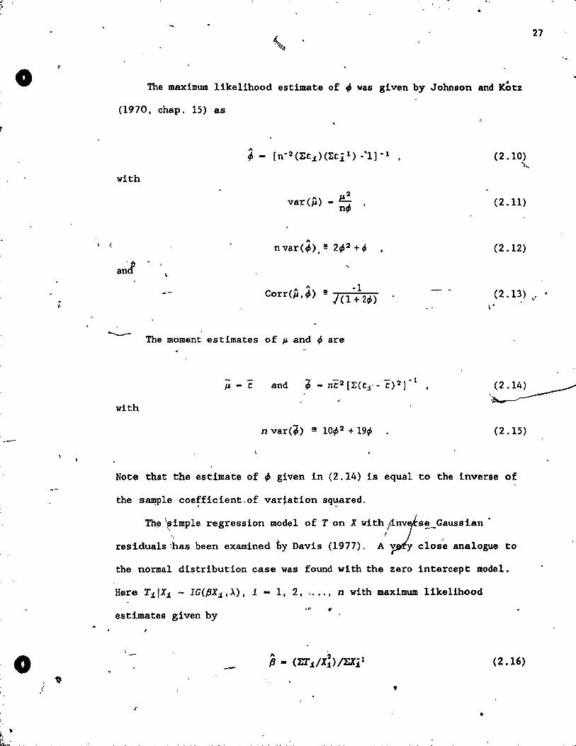
The maximum 1ike1ihood estimate of ~ was given by Johnson and Kôtz
(1970, chap. 15) as
with
an'! -
~ var(~) - nq,
(2.10) \...
(2.11)
(2.12)
27
1\" II! -1 Corr(JI,q,) - J(l + 2~) (2.13) t?
\'
The moment estimates of p and ; are
JI - t and 'j, - --1 - nt 2 [t(tj · - t) 2] ,~
with
n var(~) !! 10~2 + 19q, (2.15)
Note that the estimate of ~ given in (2.14) is equal to the inverse of
the samp1e coefficient,of var~ation squared, ", -
Th~ \~imple regression mode1 of T on X with jinv,-fS!_GausSian .
residua1s ;has been examined &y Davis (1977), At ~ c1os-~ analogue to
the normal distribution case was found with the zero intercept model.
Here T.1IX.1 - IG(PXi,À), 1 - 1,2, o •• " n with maximum 1ikelihood
estimates given by
(2.16) -,
" •
1 :-i, ,
--
" ,L \ ,
• -'.
y
", 't:-. ,-, "(-1 ... ,
28
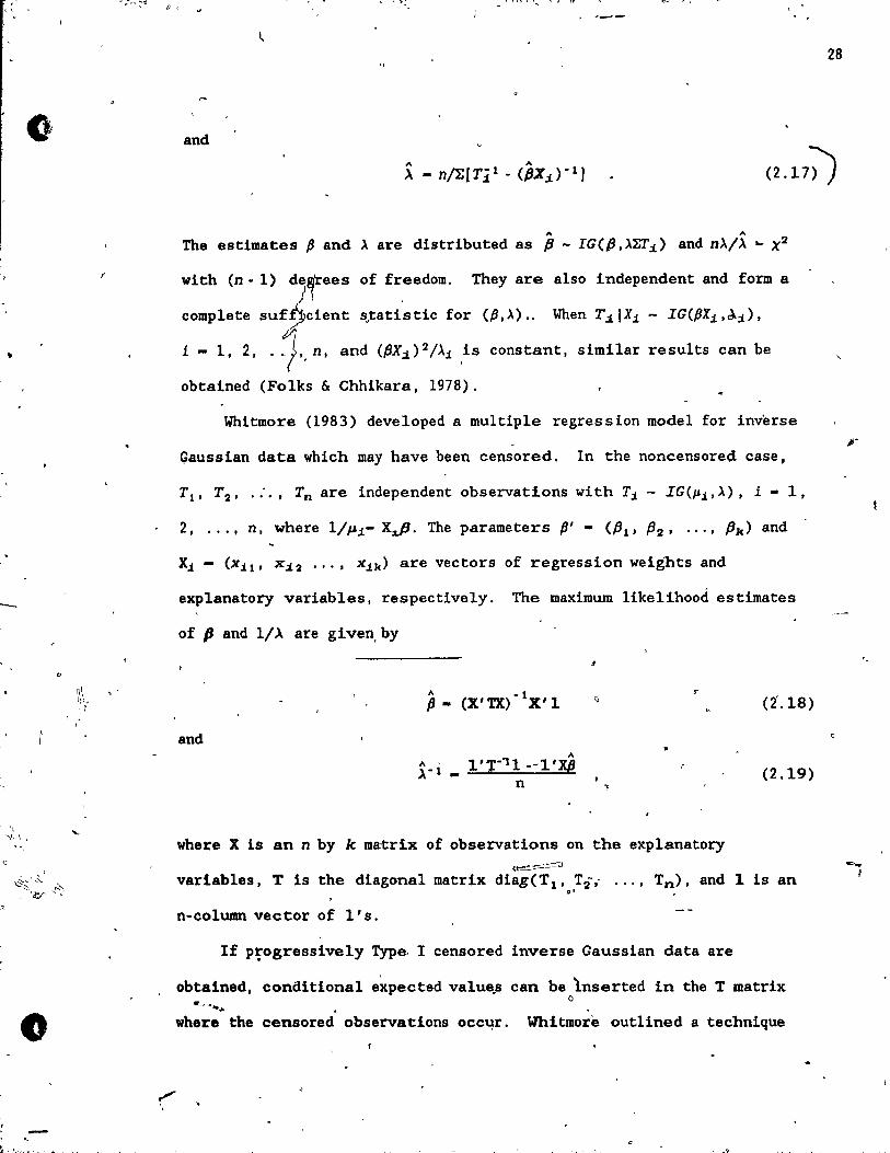
and
(2. 170 A A
The estimates {J and À are distributed as P - IG(P, À'ZI':J.) and n>./>. ... X2
with (n - 1) datees of freedom. They are also Independant and form a
complete sUf6cient s,tatistic for ({J,À).. When T:J.IXj - IG(PX j ,~i), 1 - l, 2, .),. n, and (PXi)2/Àj is constant, similar resu1ts can be
obtained (Folks & Chhikara, 1978).
Whitmore (1983) deve10ped a multiple regression model for inv~rse
Gaussian data which May have been censored. In the noncensored case,
Tl' T 2 , .'-., Tn are independent observations with Tj - IG(l1j,À) , i - l,
2, ... , n, where l/I-'j- XJJ. The parameters {J' - (PlI P2 ' ••• , Pk) and
Xj - (Xjl' Xi2 ... , Xjk) are vectors of regression weights and
exp1anatory variables, respectively. The maximum likelihood estimates
of fJ and 1/>. are gi ven, by
(2'.18)
and
n (2.19)
where X is an n by k ma1:rix of observations on the explanatory
=== variables, T is the diagonal matrix diag(T l' T 2~" ... , Tn ), and 1 is an .. n~~olumn vector of l' s.
If ptogressively Type. 1 censored inverse Gaussian data are
obtained, conditional e~pected value.s can be lnserted in the T matrix ............... o
where the censored observations occ~r. Ybi tmore outlined a technique
'.
o
o
" ,
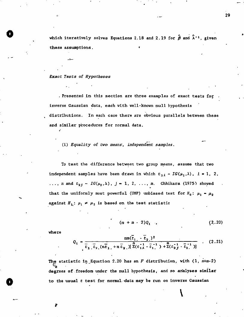
" " A which iteratively solves Equations 2.18 and 2.19 for fJ and .\ -1, given
these assumptions.
Exact Test=s of Hypotheses
. Presented in this section are three examples of exact tests for
inverse Gaussian data, each with well-known null hypothesis
distribut:ions. In each case there are obvious parallels between these
and similar ~rocedures for normal data. ('
(i) Equality of two meanS', independént samples.
To test the difference between two group m,eans, assume that two
independent samples have been drawn in which t~i - IG(}Jl'>') , i - l, 2,
... , n and t 2j - IG(1-'2'>-) , j - 1,2, ... , m. Chhikara (1975) sho~ed
that the uniformly Most powerful (UMP) unbiased test for Ho: }J1 - 112
,against Hl,: 1-'1 '" 112 is based on the test statistic
(n + m - 2)Q1 '.
~here
(2.21)
The statistic in Equation 1.20 has an F distribution. with (l, n+m-2) ~, --
degrees of, freedom u,nder the null hypothesis. and so arialyses simhar
to the ususl t test for normaL-data May be run on inverse Gaussian
\
29
... 1
~_._---
" ' , ,
"
o
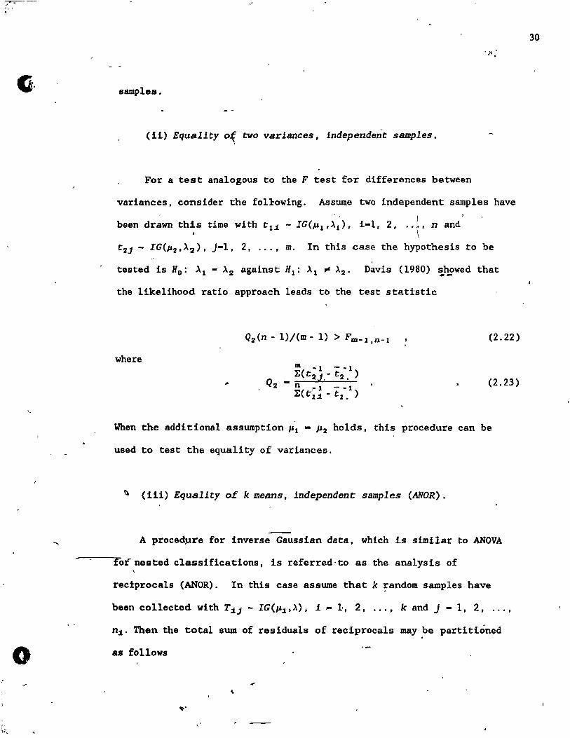
samples.
(11) Equallty o{ two variances. independent samples.
For a test ana1ogous to the F test for differences between
variances, conslder the fo1xowing. Assume two independent samp1es have
been drawn thls time with t: 1 i - IG(PI ,>'1)' 1-1. 2, .. ~, n and'
t 2 j - IG(1'2' >'2)' )-1. 2. . ..• m. In this case the hypothesis to be
Davis (1980) showed that .. -the 1ikelihood ratio approach leads to the test statfstic
Q2(n - l)/(m - 1) > Fm-l.n-l (2.22)
where
(2.23)
When the additional assumption 1'1 - P2 holds. this procedure can be
used to test the equallty of variances.
(IIi) Equality of k mesas, independent: samples (ANOR).
A proce~ure for Inverse Gaussian data. which ls siml1ar to ANOVA
for nested classificatIons. ls referred' to as the ana1ys is of
reciproca1s (ANOR). In this case assume that k ~andom samples have
been co11ected with Ti) - IG(lIi,À) , 1,.. 1:. 2 •...• k and J - 1.2 •...•
nj' Then the total sum of residuals of reciprocals may ~e partitiôned
as follows
...
30
o
o
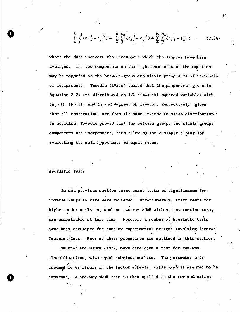
(2.24)
where the pots indicate the inde~ ove~ which the samples have been
averaged. The two components on the right hand side of the equation
may be regarded as the between_group and within group surns of residuals
of reciprocals. Tweedie (1957a) showed that the Fomponents given in
Equation 2.24 are distributed as l/À times chi-squared vàriables with
(n.-l), (k-l). and (n.-k)degrees of'freedom, respectively, given'
that aIl observations are from the same inverse Gaussian distribution.'
In addition, Tweedie proved that the between groups and within groups
components are independent, thus allowing for a simple F test for , \
evaluating the null hypothesis of equal means. (
Heuristic Tests
In the previous section three exact tests of significance for lI,'
inverse Gau~sian data were reviewed. Unfortunately, exaé~ tests for
higher order analysis, such as two-way ANOR with an interaction term,
are unavailable at'this time. . c
However, a number of heuristi'c tests , ,
have been dev~loped for complex experimeI"ital designs involving inverse'
Gaussian :data. Four af these procedures are outlined in this section.
Shuster and Miura (1972) have develaped a test for two-way
classifications, ~ith equa1 subc1ass numbers. The parameter p 18 , assurned to be linear in the factor effects, while À/p2 .. is assumed to be
Il
constant. A one-way ANOR test Is then applied to the row and column
r
31
, ,
\
. ,
, . , .. " ..
totals to test for main effects., Evidence of interaction between any~f
two columns is then achleved by testing for the equa1ity of means ln a
two samp1e prob1em. The total significance 1evei which re~u1ts from . '
perfotming all of thes~ tests ls calcu1ated by using Fisher' s method -of
combining tests (Fisher, 1958).
Thi.s procedure has two maj or' dra~bac,ks. First, 'Fisher' s method of 1
combining tests assumes independence '~ong indlv~dua1 tests. Thus,' ~ .
disjoin~ data sets are requited a~d, so many observations per ceU are
needed. The 'se'cond problem concerns the assumpt~on of 'constant ')./p2. • 1 "
As was mentioned eaÎ'lier in this chap'ter; a con~tant coefficient of
variation (i.e.,' /(JJ/'A» 'across groups is more Uke1y to be found wl:ten
1atency data are anàlysed. "
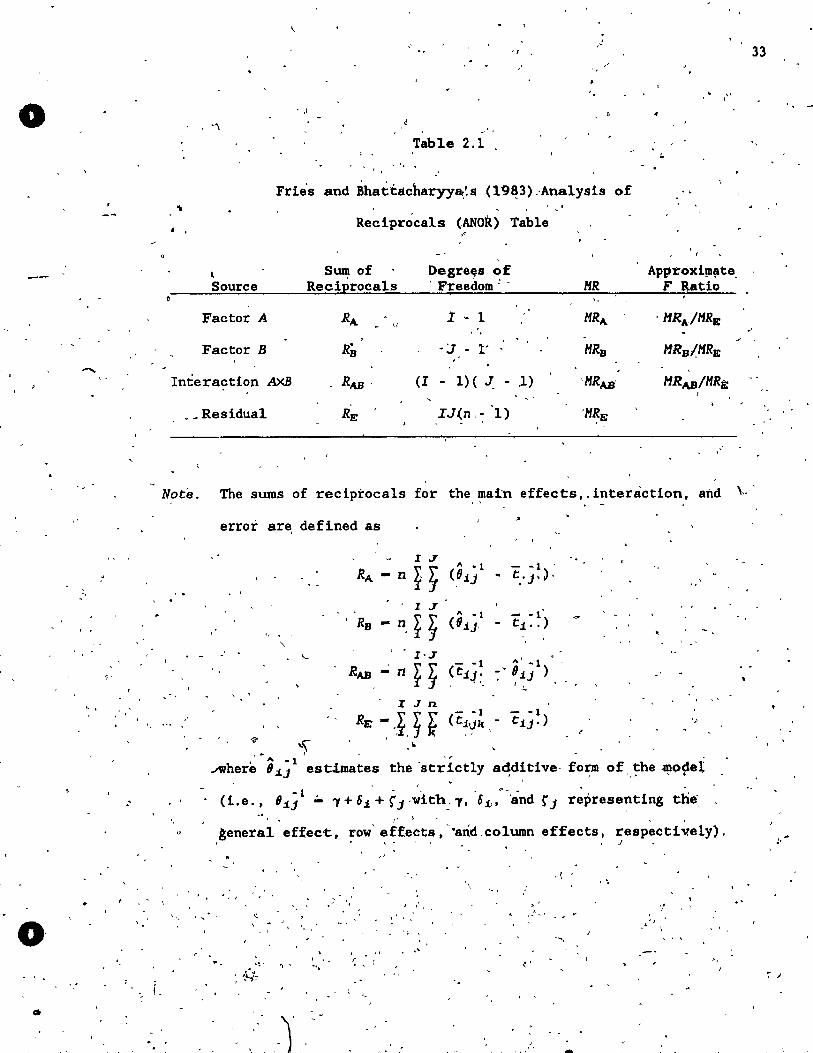
Fries and SfîattacharyYa (1983) have deve10ped mo~e sophistlcated ,
1: procedures for ba1anced two-factor experiments. They assumed that 111S:
-)
ls linear in the main effects while ~/À ls constant across a11 leve1s, 1 • ,
of' factors. ~eir ANOR tabl~, using ~aximum 1ik~lihood estimates is , ,
shown in. Table 2,.1. Fries "and Bhattacharjya a1;;0 produced a similar "
appioach based ôn -unbias~d estimation' t~rough a least squares approac:h.
, "
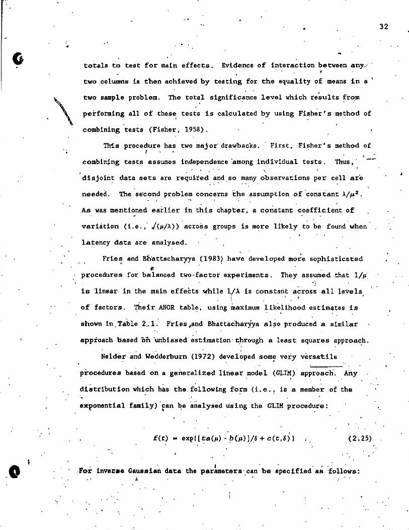
Ne1der and Wedderburn (1972) deve10ped some very versatile . '
prooedures ba$ed on a generaUzed linear .model (GUH) approach. # . ', •
distribution which hils the. fo11ow:Lng form (i. e., is a member of the '. . ..
"
exponentia1 fami1y)' fan ~e 'ana1ysed ùslng the GLIM procedure:
, ,
f(t) 1
exp! [ta(,,) - b(p) liS + c(t r 6) } ) 1 • ' ••
(2.25)
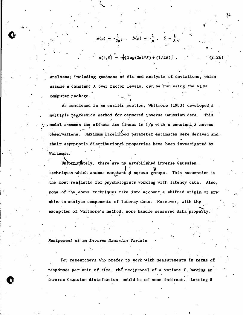
~ .For inveJise Gaussian data the parameters·.c~n be specified as follows:
.!.
32
o
-
,"
l'
, .
. '
0-
. " 33 -,
"
. ., 1
, ,1
-' , Table 2.1
l ,
, "
Frie's and Bhatt:8.charyy~~$ (19~3) _'Ana1ysis of
Reciprocals (ANOR) Table ,.,
, Sum of Degrè~s of Approxi!1l~te, Source Recit>roca1s ' Freedom: - HR F Ratio
Factor A RA ,; 1 '- 1 HRA, . HRAjHRE , , "
Factor B R~ . 'J - l' HRB HRB/HRE
Interaction AXB RAB ' (1 - 1)( "- - ,1) 'HRAJî HRA,B/HRfi: - '
. _ Residua1 RE IJ(n '~ 1) 'H~E
"
Note. The sums of -reciptoca1s for the main effects" interàct1on, and \'"
erroi' ar~ defined as
l J "
, ' q~
'- -1 - ~1 ' RA -n (8 i j t:J' ).
l J - -1' n, t ~ " -1 , RB (Oil- t i .. )
, .
l·J ,-' ~ 1 <
~nt~ - -1
RAB ~ t 1.j:. : ~ 0 iJ ) '-',
l J n ' '
RE ~I~ ~ - -1 - -1
(ti'JI« tiJ' ) '.' , "
~ ~\ , • 1
• '" -1 A1here (J iJ estimates the 'strict1y a~ditive. fo~ of ,,~he -I!lo~el 1 1'" f
. (i.e .• (J i/ .:. 'Y + 6 i + r j'wlth __ 'Y, 6 i. ,P "and r j represe~ting the, " \
tenersl effect. row' effects • -"and, column effects, respecti vely) . J ~
. ,
, , ( , . , , "
r • . 1 _
-',
. , ." .
, '
Ir .:. .. '
> .t" ,. ~ ,
_ 1 ~ •
. ' ,
. ~ ,. .
," 1
_. l,
, '
"
, "
,-
/ ,,,.
." ... b(p) l .p, '
" ,
'. (2.26)
, >
Analyses; including goodness of fit and analysis of deviat~ons, which
assume a'constant À over factor levels, can be 'run uslng the GLIM
computer package. "
r
A's mentioned in an eat:lièr .section, Whitmore (1983) developed, à
multiple ~egression method for ce~~ored inverse Gaussian datà. This .~ ,
,model assumes the effects are Ùnear in l/p with a constant., ~ across • ~ - t ' •• . ~ - ).
observations. Maximum likelihood parame ter estlmates were,derived and. , ,
their asympt~tic ~is~ributionft p~operties have been investigated by
Whitmore: .
, U~~t~lY, there"are no
J techniques which assume constant
..".
established inverse Gaussian _
VI tP àçross groups '/ This, assumptlon 19
the Most rea~istic for psychologists working with latency data. Also, ,
. none of the. above tech~iq~~s tak~ into account. a shifted origin ot are'
abl~ to analyse components of latency data. Moreover, with th~ . ......
exception of Whitmore's method, none handle censorei data, properly.:
"
Reclp~ocal of an Inverse G8us~lan Variate
For researchers who prefer to work wlth measurements rn terms of
responses per 'unit of tlme, th' r~clprocal of a variate T, having an "
inverse Gal\lSsian dlstributio~, could be of some int'érest. Letting R
3-4
. ! .
o •
.. . . ,
\'
o , ,
"' . d
-'
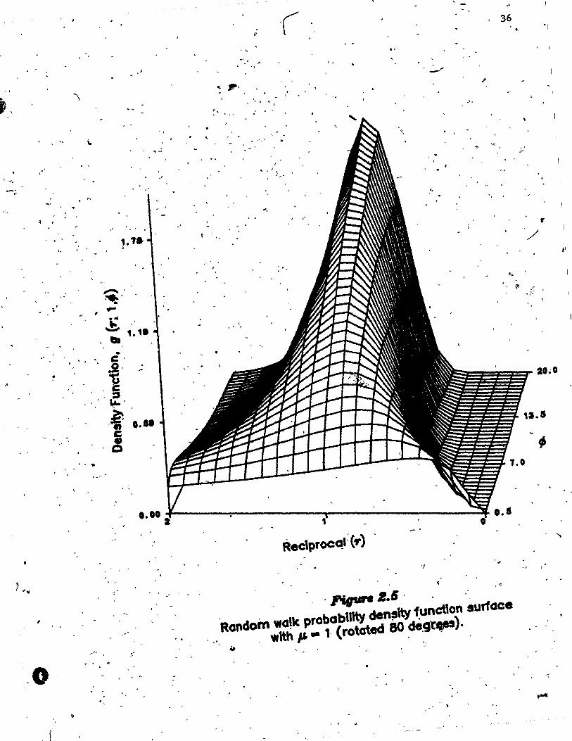
denote this random var;l ab le , the corresponding probabUity density , ,
function is
, -(f"t)% ~xp [-~(~r' + p
1r - ,2)] . (r, P, ;>0);'
, "
'(2.27) .' .
:where f(J'n1,;) ls thè usual inverse Gaussian pro'bahi'lity qensity
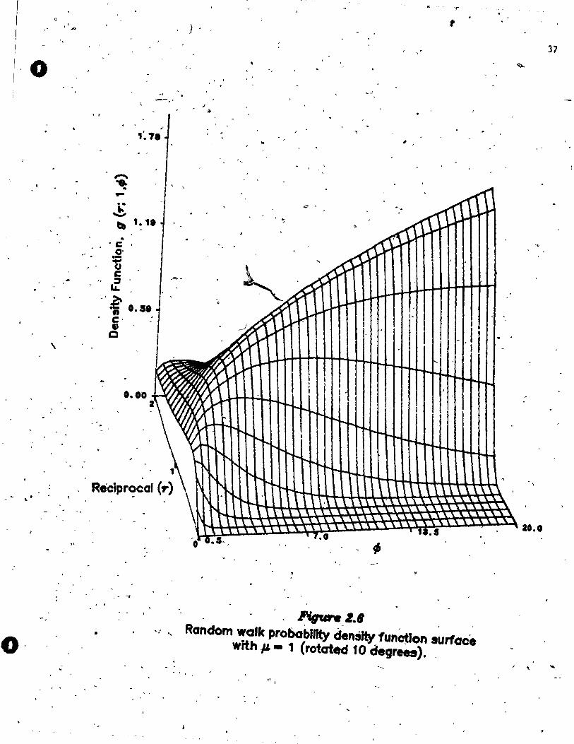
funètion. This ~istrib4tion i8 ,usuàlly'cailed the Random Walk
distribution (Wise, 1966). Figures 2.5 and 2.6 contaln plots of·random , ..
walk p;robabiUty_ de.nsity surfaces, with fixed par:ametêr l' '-'1 and '..,
varying ~, from two differ~~t views. . ,. .
Tweedie (1957a) found,that the mode of this distribution ls
lçcated at ,.
r
(2.28) ...
The, cumùlant generat~ng funcd,on .of r is givet\ by
. . -1 l' -1
. ~(l - i[1 + 2y(",;)" )} - '2log[:4+ 2y(p.;) ) (2.2,9)
:rweedie 'noted that -$:his indlcates that the Randorn Yal!< dis,ttibution ean
be regarded as, a convolution of an inverse Gaussian (with the sarne
value of À but p replaced by l/p) with- an independent chi-square
distributi,on times l/l.-
Mos't of the basic properties of the variate R follow easlly froJJl.
~,
35
);
:;--~', t'
" . , '
,.' . .' ". '-' o
, . "il t .. ' •
. ' '/
Il
~,
\'1 ,
'"
• 'il
20:0
" ,1
o."
, .. T.O
0.00 ~--~---T--~/~.------;r~~--~~------~~~ Reclprocqf (f')
','
, c
, ,l'ir'" ~.6 RClllcIoIn WO!k probabtlllY cten!SItY f,uncllon surface
"'.. . _\th ~ - 1 (rototed 80 deg-,)' •
1
. . r
'0·
, Recipr~~ol Cr)
_~-ao.o Il
• l'igutw Z.I
'-, '. Rondom walk probobllJty chtnsfty fun~lon surface with # - 1 (rotat.cf 10 degrees). ,
..
, ,
o
. , " ,H
0 , ,., J
~, tl,- ,
Di' \ .. V.l • , .. "<..
. . i
tFose' of the. inverse Gaussian. For: exemple, Tweedie (1957a) showed . \ .
that in general, the partition of reciprocals~or inverse Gaussian
variates ,œay be Writ~én.as
. ,
, . (2.30)
,- '
where ;(t) t- 1, and the three sums 'are eaeh distributed as l/À times
ehi-square.with (n. -1), ~n. ,- ,k) and (k - 1) degrees of freedom;
respeçtively. Letting·~(t) - r, the sum beeomes
-
\
.. r (2.31)
(- -where ri. and r are harmonie means of the values of rij' As discussed
in chapter 1, the harmoniç Mean ls a reasonable measure to use when .
responses per unl.t of time are averaged .
, . .. . . . ,
38
!
o
o
/
Chapter 3
Reaction Times
. '.
Basic Issues
, The study of reaction time, defined as the minimum time between a
stimulus onset (or offset) and a response, has a long history within
psychology. Ribot (1900) suggested that Helmholtz (1850) was the flrst
to design a reaction time exper~ment in order to estimate the speed of
neural 'transmission. An early study~pn the nature of decision . 1
processes was conducte~ by Donders (1868) which invo1ved~he comparlson.
, . of simple and cholce reaction times.
A number of investlgators have studied the appropriateness of
various theoretica1 distributions for modeling reaction time data.
These inc1ude the gamma (e.g .• Christie & Luce, 1956; McGill. 1963),
double monomial (Snodgrass, Luce, & Ga1anter, 1967), 1ognorma1 .. (Woodworth & Schlosberg,' 1954), Pearson type V (Thomas, 1969), and
double exponentia1 (Green & Luce, 1973; Wande1l & Luce, 1978).
Unfortunat~ly., no ,!heoretical distribution has beerl found which
.. .
accuratelyaccounts for aIl the'inherent characteristics of reactlon
time data'(Burbeck & Luce, 1982).
Other investigators have developed stochastic models for reaction
1
times based on asswnptions about the underlying psychologieal proeessea .'
which produc~ the observed response. Most of these faU into one of
_. -
39
1
o
.-'/
. ;..-.0..-- .
--'three basic classes of modela: varied-state, counting, and random walk •
1 (Townsend and Ashby, 1983, chap. 9). These a11 aSSUJDe that sUbjects"
IJ
are not perfect in terms of their performance and attempt to explain
how and whep response errors occur.
The objective of this chapter is to discuss various attributes of
reaction time data and whether the inverse Gaussian distribution is a
reasonab1e mode1 for them. Two extensive sets of sample data are
discussed
Ssmple Data
5
along with the results from fitting basic inverse
normal models to them. The sections random walk models
ctlons ~ follow present theoretical arguments for
inverse Gaussian distribution. Finally, modeling
with convolutions is discussed.
"/
The sta~istical estimation procedures developed in this'thesis
were applied to two extensive sets of reactio~ time data. The first
set contains simple reaction times which were collected by Dr. S. L.
Burbeck (1979) as part; of his Ph.D. dissertation, University of
California at Irvine. The data were collected from three subjects at
the Psychophysical ~boratory, Harvard University. The test stimuli
used vere the offsets of weak pure tones masked by wide-band noise. In
" addition, subj ects' minlD\um reaction times were obtained in a ~eparate (
experillent which utilized the ,offset of a loud, wide-band noise. In
both cases subjects responded by p~essing' a microswitch. In order to
. '
40
0-
o "
1 . . i. '"; ;"... ~~ \. <t .. J I~ • _.- ~~ -.--,
minimize an~ici~t\pn responses_~xponenttaI1y distributed ~andom
foreperiods were uS,ed.
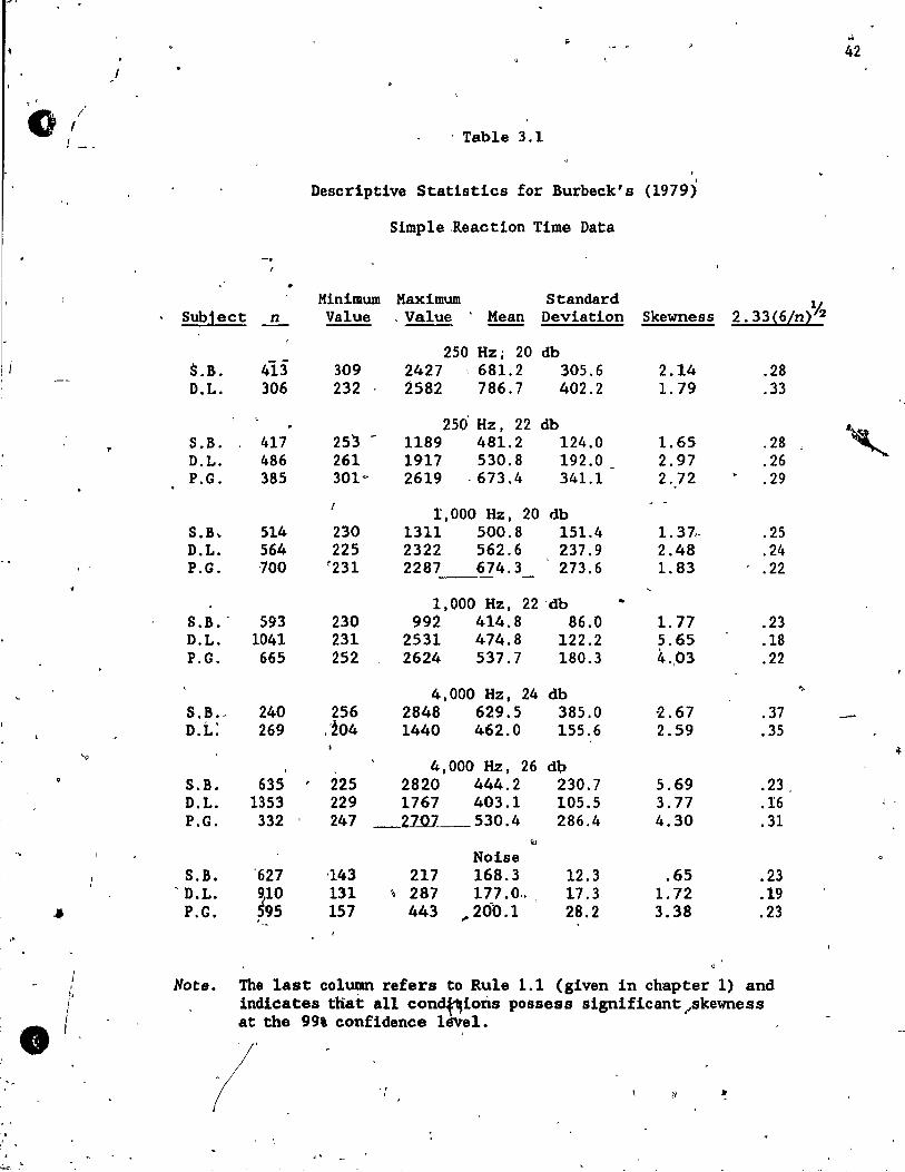
Descrip~ive statistics for Burbeck's data are found in-Table l.l.
Note that no data was available for subj ect P. G. in the 4,000 Hz, 24 db
(, condition. AIso, as the distribution of times for subject P.G. from ~.
: the' 250 Hz, 20 db condition was found to be atypical, they were not
~ considered in this thesis. The last "Column contains values pertaining -to Rule 1.1 given in chapter land indieate that aIl conditions yielded
" highly skewed data. Further details of the Burbeck' s experimenta1
method and results can also ber found in Burbeck and Luce (1982).
The second set contains ,two-choice reaction times which were
41
provided through the courtesy of Dr. S, W. Link. The unpublished data 0
" were collected in 1977 at McMaster University from eight subje~ts.
t, "
Distances between two dots presented visually were judged to be long or
short: by tI:te observers. Ei ther a fixation point or standard length was)
presented before the test stimuli were shown. AlI trials were subject ".
initiated and feedback as to the accuracy of each response was provided
after subjects' choices had been made,
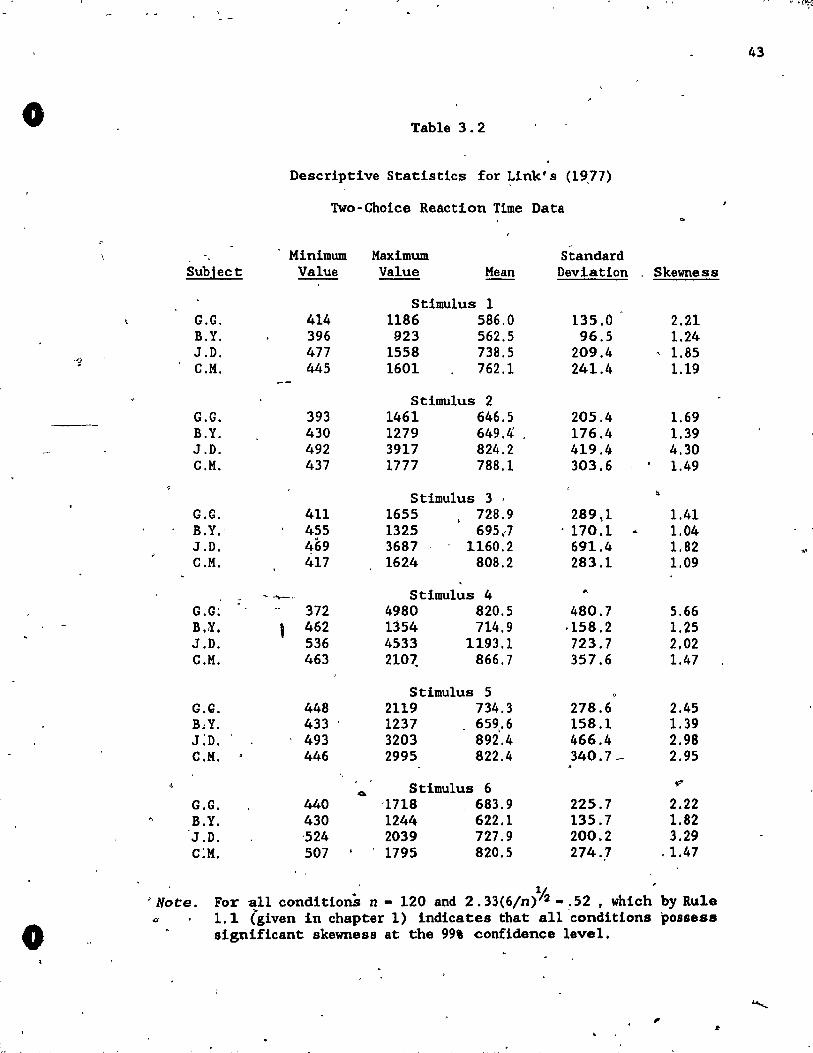
Table 3.2 contains descriptive statistics for Link's data. While
response times were found to be noticeably longer on average then those
- from Burbeck' s experiment, the sarne high levels of skewness are ,
ev~d~nt. Note that, except for some data c1e~ning proc~dures (Burbeclt
& Luce, 1982), no censoring took plaèe in either experiment.
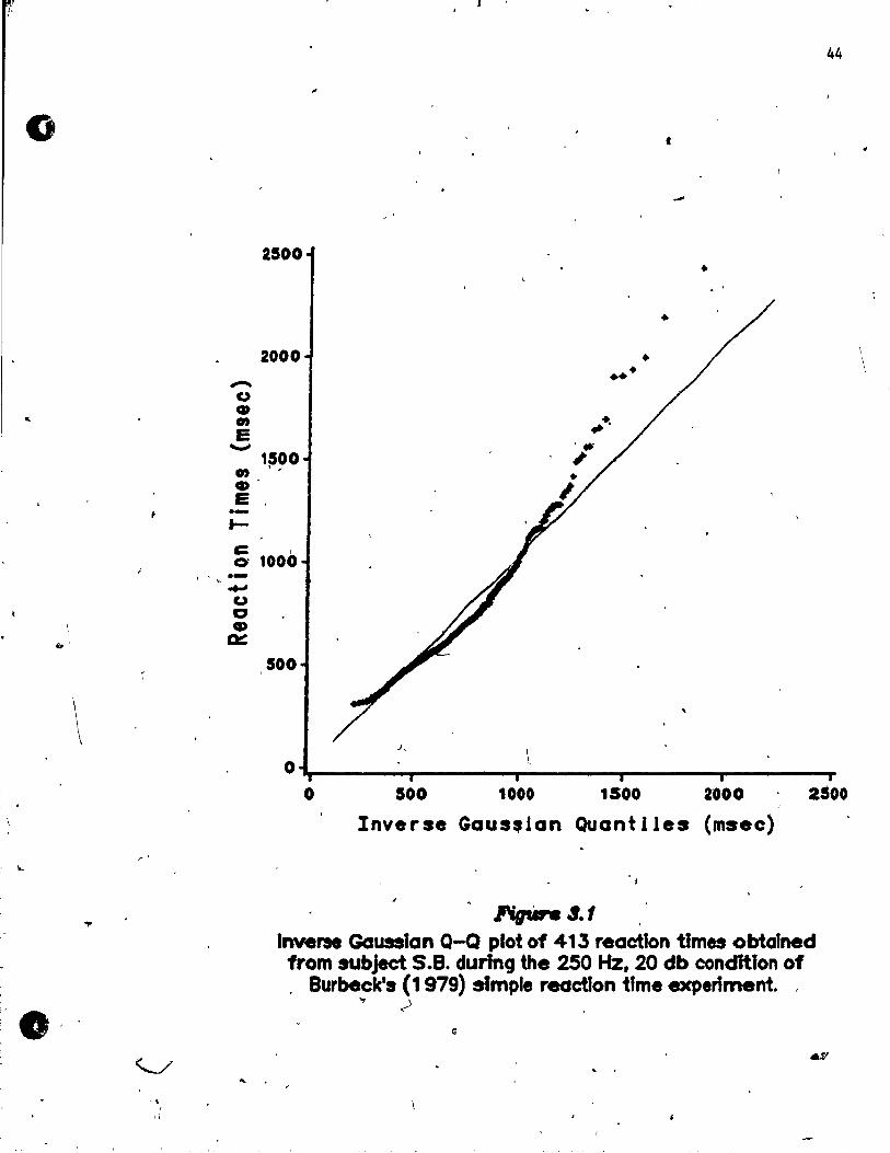
1 An i~rse Gaussian Q-Q plot, based on maximum likelihood l,
parame ter estimates, o'ï subject S.B.'s"responses during the 25 Hz, 20 l
db condition of Burbeck' s experiment is found in Figure 3.1. "'rhe trend
, . 1
,
..1,'-
.:.
42
,
0/ ! --
, Table 3.1
Descriptive Stat1stics for Burbeck's (1979)
Simple ,Reaction Time Data
Minimum Maximum Standard 2.33 (6/n)% , Sub1ect -.!!.... Value , Value ,
~ Deviation Skewness
4ïj 250 Hz i 20 db
il S.B. 309 2427 ' 681. 2 305.6 2.14 .28 D.L. 306 232 2582 786.7 402.2 l. 79 .33
250' Hz, 22 db , S.B. 417 253 - 1189 48l.2 124.0 1.65 .28 D.L. 486 261 1917 530.8 192.0 2.97 .26 P.G. 385 301" 2619 - 673.4 341.1 2.72 .29
! 1,000 Hz, 20 db S.B .. 514 230 1311 500.8 151.4 1. 37,.... .25 D.L. 564 225 2322 562.6 237.9 2.48 .24 P.G. '700 ~231 2287 674.3 273.6 1.83 .22 ----
1,000 Hz, 22 'db • S.B. - 593 230 992 414.8 86.0 1. 77 .23 D.L. 1041 231 2531 474.8 122.2 5.65 .18 P.G. 665 252 2624 537.7 180.3 4.,03 .22
4,000 Hz, 24 db "
S.B," 240 256 2848 629.5 385.0 -2.67 .37 D.t: 269 ,'204 1440 462.0 155.6 2.59 .35
'0 4
4,000 Hz, 26 d~ S.B. 635 225 2820 444.2 230.7 5.69 .23, D.L. 1353 229 1767 403.1 105.5 3.77 .16 ' '
P.G. 332 " 247 --.1JJl1_ 530.4 286.4 4.30 .31 YJ
Noise S.B. '627 143 217 168.3 12.3 .65 .23
- D.L. ~10 131 , 287 177.0 .. 17.3 1. 72 .19 .. P.G. 95 157 443 ... 260.1 28.2 3.38 .23
"
1 Note. The last eolumn refers to Rule 1.1 (given in chapter 1) and !.
indicates t~at all cond~ioôs possess significant~skewness /
• 1 at the 99% confidence lè"1e1 .
/'
1 \ Il ~
, , \ , . " -1.;, ,1>
; ,.-
43
0 Table 3.2
Descriptive Statistics for Link' s (19}7)
Two-Choice Reaction Time Data
-Minimum Maximum Standard
Subject Value -- Value Mean Deviation Skewness
Stimulus 1 G.G. 414 1186 586.0 135.0 2.21 B.Y. 396 923 562.5 96.5 1.24 J.D. 477 1558 738.5 209.4 ' 1.85
il C.M. 445 1601 762.1 241.4 1.19
Stimulus 2 G.G. 393 1461 646.5 205.4 1.69 ---- B.Y. 430 1279 649.4 . 176.4 1.39 J .D. 492 3917 824.2 419.4 4.30 C.M. 437 1777 788.1 303.6 1.49
Stimulus 3 ' ~
G.G. 411 1655 728.9 289\1 1.41 B.Y.' 455 1325 695 .. 7 . 170.1 1.04 J .D. 469 3687 - 1160.2 691.4 1.82 ~,
C.M. 417 1624 808.2 283.1 1.09
Stimulus 4 -. ..... -"\0-0-- ~
G.G: 372 4980 820.5 480.7 5.66 B.~. , 462 1354 714.9 ·158.2 1.25 J .D. 536 4533 1193.1 723.7 2,02 C.M. 463 210~ 866.7 357.6 1.47
Stimulus 5 G.Q. 448 2119 734.3 278.6 2.45 B.Y. 433 . 1237 659,.6 158.1 1.39 J:D. 493 3203 892.4 466.4 2.98 C.M. 446 2995 822.4 340.7_ 2.95
Stimulus 6 .p .a-
G.G. 440 '1718 683.9 225.7 2.22 B.Y. 430 1244 622.1 135.7 1.82 J.D. '524 2039 727.9 200.2 3.29 C:M. 507 . 1795 820.5 274.,1 ,1.47
. l '
, Not:e. For aU conditionS n - 120 and 2. 33(6/n)~ - .52 , which by Rule <1 1.1 (given in chapter 1) indicates that aIl 'conditions possess
0 significant skewness at the 99' confidence level.
, . ,
o
...
\
.,.
r'
, , ,
"
"" CJ CD ., E
-..."
2500
2000
1500 ., ,~
CD E, .-f-
~ 1000
500
r' . ,
44
1
• . '
J,
~ O~ ______ ~ ______ ~ ______________________ __
o 500 tOOO t500 2000 2~00
Inverse Gaus.lan Quant 1 les (msec)
l'igùre I.t Inverse Gauss1an Q-Q plot of 413 reactton t1mes obtalned trom subject S.8. during the 250 Hz, 20 db condH.lon of . Burbeck's (1979) simple reactlon t'me experiment. ,
... .--l
o
,
o
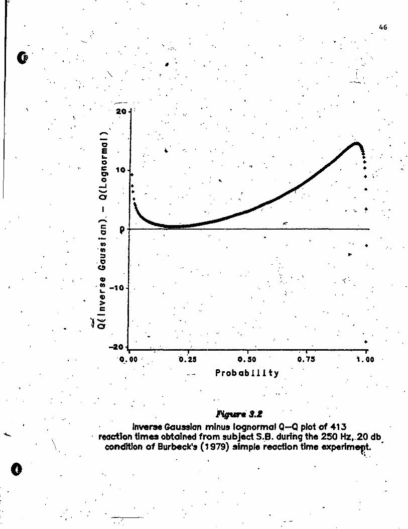
is similar to- that found in the lognormal 'Q-Q plot of the same data (in
Figure 1. 3) as the residual Q-Q plot in Figure 3.2 indlcat,es.
C;omparhons of inverse Gaussian versus lognormal. ,fits ,for aIl
\ ~ -conditions in Buroëë1('s experiment are found in Table 3.3. Clearly_
there is Little difference between the two distributions in terms of
fitting the data using maximum likelihopd estimates of the
corresponding parameters. Note that the Pearson' s chi -squar,e vaIlles
repo~ted in this thesis are intended for compar~son -purposes only.
They do not indicate whether particular distributions May or may not be
assumed for" purposes of statistical analyses.
Table 3.4 contains maximum likeÜhood estimates of the population .
means, wi th corresponding confidence intervals, based on assumptions -of
underlying inverse Gaussian and lognormal ;dis'tributions. Note that the
inverse Gaussian estimates of l'are equi valent to the sample means.
Maximum likelihood estimates of the' popufation standard devlations
and skewness assuming normal, inverse Gaussian and lognormal ~\
---- ~ \
distributions are found in Table 3.5.' Underestimat~--t:he sample , ~ -
standard.-deviation and skewness by bQth--t1iêinverse Gaussian and ~~
lognormal distributfons indicate that neither distributioQ models .the
data very weIl.
-Similar resul ts for the data from Link' s two - choice experlméht are
found in Tables 3.6, 3.7, and 3.8. Clearly both the inverse Gauss'ian
and lognormal distributions are limited in their ability to model ,
either simple or two-..choice réactiO'n times. However, modifications to
thè probability density functlon defini tion can,f improve the inverse
Gaussian modeling capabilit1es substantially. Such modifications are
. -
....
45
, .
"
------
0' .
l '
1,
"
\
o
"-
--20
,.... -0 E ... 0 e 10 0-0
-1 ...... 0
,.... C P QI .-en
'0)
:::s . ., C)
CI)
,., -10 '-CD > C
10
'-
"
-\ '
, , ..
-, • , ,
1
• ~O~ __ ~ ____ ~ ________ ~ ________ ~~ ________ ~
'0_.00" . 0.50
Probab 111 ty
i'rigun a.~
0.'75
Inverse GGusslon minus lognormal g-Q plot of 413
1. 00
46
reactton tlmes obtalned from subject S •. B. du ring the 250 HZ •. 20 db .. condition of Burbeck', (1979) simple reactJon tlme experim~t.
t.
"
, ..
<.
. 0
_' _---~ <J-
\ .. ~ -
, ' 4
Table 3.3"
, ,
- "
--
• 0
,Maximum Like1ih~oa Estimates of Inverse Gaussian and Lognorma1 ", - , , , '
Parameters, and Chi-Square Good~ess-of-Fit Kea~ures . - ':,
for Burb~ck's (1979) Simple Reaction Tim~ Data
--...
, 1 Inverse Gaussian 'Lognormal Subject .2L e. ~ x 2 fl. W x2
,
~ 250 Hz, 20 db
S.B. 413 681.2 6.66 42.6* 6.45 ".373 42.8* D.L. '306 786.7 4.67 29.8 6.56' - .440 31.5
250 Hz, ;2~"~: 1
l, ... ,
S.B. 417 481.2 ' * 6.15 ' .235 1 59.6* 17 .46 62.~1
I?L. '486 " ' 530.8, '* 6.23 69.1* 11.14 74., .291-t, - P.G. 385 673.4 6'.26 84.0 6.43 .381,\ 81.0*
\ 1 , 000 Hz" 2 db
. S.B, 514 500.8, Il.~9 30.4 - 6.18 .28~ ,30.7 D.L. ,-' ,564 562.6 7.61 50.8* 6.27 .349 ~1...9'1!
'P.C. 700 674.3 7,.06 " -
45.7* 6.44 .363 -~8.3*
1,000 Hz, 22 db 1 S .. B. 593 414.8 Z6. :t9 '< 37.7* 6.01 .1~3 '~ D.L. 1041 474.8 21.59 70.2* 6.14
47 , '
P.G. 665 53,7.7 13.24 73.3* 6.25 :2Ü ( 59. * . .2671 72.3*./ --"
! -; - . . /,
4,000 Hz, 24 db -- /' ~
-90.2* - S'.B. 240 629.6 4.28 85.2* 6.32 ( .455 D.L. -269 462.0 Il.99 40.5* 6.09 \ .281 f 42.9*
/.
-- - ----- ~- -"--- - \
4,;000 Hz, 26 db S.B~ 635 0444.2 '9.08 205.2* 6.03 .31'2. 167.8*
," D,.L. - 1353 403.2 20.89 113.5* 5.97 .214 90.7* P.C. 332' 530.4 6.99 . 90.0* 6.19 .357, . 85.0*
~ Noise S.B. -627 l6à.~ 191.81 143.3* ) 5:12 .072 143.4* ,D.L. 910 177.0 117.16 109:6* 5.17 .092 'gr.. 1* , , P.G. 595 '200.1 66.27 - 153.2* 5.29 . .122 '153~2'1!
* p. < .O~, with 17 dE for 'aIl conditions .
••
',,-,-
(
) , "
.(
....
~ ,
0
"' ... ' 1 Table 3.4
M~xim~ Llke~ih~od Éstimates of Population Means,'with
Subject ...!!...
S'oB. .. ,'413 D~ I,~ 306
S.~. 417 D.L~ 486 P.G.- ' 385,
S.B. 514 D.L. 564
, P.G •. 700
S. B.-- 593 D.L'. 1041 P.G. 6.65
S.B. 240 D.L. 269
S.B. 635 D.L. 1353 P.G. 332
, ·S .~; 627 D.L. 910 P.G. 595
, . Corre~ponding Confidence Intervals. As~umlng
Inve~se Gauss~an and,Lognorma1 Distributions
fdr 'Burbeck' s (197.9) Simple Reaction Time Data,
-, Confidence Confidence t rG ,. Interval {95%} t LN !,nterva1 ~95%~,
. ' " 250 Hz, 20' db
681:2 (656.6, 707.7) 676.3 (652.4, 701.1) 786.7 (747.9-,' 829.8) 781.0 (743.4, 820r5)
·250 Hz, 22 db 481.2 (470:4, 492.5) '480~ 6 (469.8, 491. 6) , 530.8 (517.1, 545.4:) 528.1' (514·7, ~42.0,) -673.4 (647.5, 701.4) 664,:8 (640.0" 699·n,
1,000 Hz, 20 db '-500.8 (488.6, 513.6) 500.2 '(488.1, 512.6) 562.6 (546.-2, 579.9) 559.1 (543.2, 575.5) 674.3 (656.0,' 693.6) 67,2.3 (654.4, 690.6)
1
1,000 Hz, 22 db 414.8 (408.3, 421:4) 4;1.4.5 (408.1~ 421.0) 474·8 (468.7, 481.1) 473.9 (467.9", 480.0) 537.7 (526.7, 549.2) 535~5 (524',7, 546.5)
629.5', 4,000 Hz, 24 db
(593.2, 670.6) , 617,9 (583.3, '654.5) 462.0 t446.6, 478.6) 460.3 (445.0, 476.0)
4,000 Hz, 26 db 444.2 (433.0, 455.9) 437.2 (426.7, 448.0) 403.2 (398.5, «'07.9) 402.1 (397.6, 406.8) 530.4 (509.7, '553.0) 522.0 (502.3, 542.5)
Noise 16,a.3 (167.3, 169.2) 1-68.3 (167.3, 169.2) 177.0 (176.0, 178.1) 177.0 (175.9, 178.1) 200.1 (198.1, 202.1) 200.0 (198.0 .. 201. 9)
•
48
1
, "
~
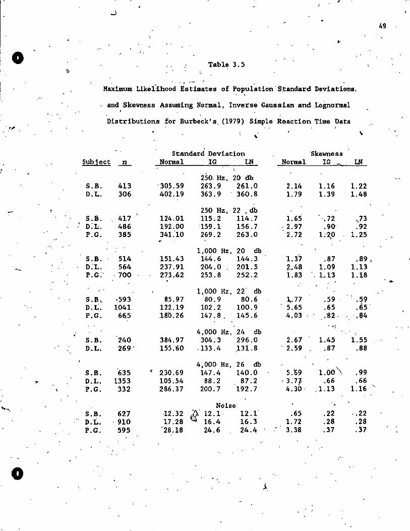
.. ", .~
.J ..
49
J'
0 ' ,
Table 3.5 -1: "
~ . ..,-....
Maximum Likelihood ~st1mates of Population -Standard De"iations.
and Skewness Assuming Normal, Inverse Gaussian and Lognormal • " '
Distributions for Burbeck' s _ (1979) Simple Reaction Time Data -,4" .. ,
. Standard Deviation -Skewness
Subject ...!L Normal lG LN Normal IG O!::o LN ; ,
250- Hz, 20 db S.B. 413 '305.59 263.9 261.0 2.14 1.16 1.22 D.L. 306 402.19 363.9 360.8 1. 79 1.39 1.48
- 250 Hz, 22 ,db S.B. 417 124.01 115.2 114.7 1.65 -.72 . .13 , D~L. 486 192.00 '159.1 156.7 -.2.97 .90- .92 P.G. 385 341.'10 269.2 263.0 2.72 1.'2,0 1.25
" 1,000 Hz, 20 db S.B. 514 151.43 144.6 144.3 1.37 .87 . 89 ~
"- D:L. 564 237.91 204.0 201.5 .2 .. 48 1.09 1.13 P.G:- ,700 Z73 • .62 253.8 252'.2 1.83 L13 1.1.8 ...
.. 1,.000 Hz, 22- db S.~,_ ·5~3 85.97 80.9 80.6 1..77 .59 ' -, .59 D.L. 1041 122.19 102.2 100.9 5.65 .65 .65 -P.G. 665 18'0.26 147.8, 145.6 4.03 ;82, , '.84
. -( . '
4,000 Hz, 24 db , S.B. 240 384.97 304.3 296.0 2.61 ,1.45 1.55
( D.L. 269' 155.'60 ,133.4 .131.8 - 2.59 .87 .88 . -
4,000 Hz, 26 db S.B. '635 " 230.69 147.4 140.0 5.~9 1.00\ .99
1" D.L. 1353 105.54 88.2 87.2 . 3 :7} .66 .66 P.G. 332 286.37 200.7 192.7 4.30- ,1.13 1.1'6 "
,,~, N61se S.B. 627 12.32 ~' 12.1· 12.1' .65 .22 ' .22 D.L. ' 910 17.28 16.4 16.3 1.72 .28 .28 P.G. 595 '28.~8 24.6 24.4 - 3.38 .37 .~7
,,' . . , ..
0 . .
f,.
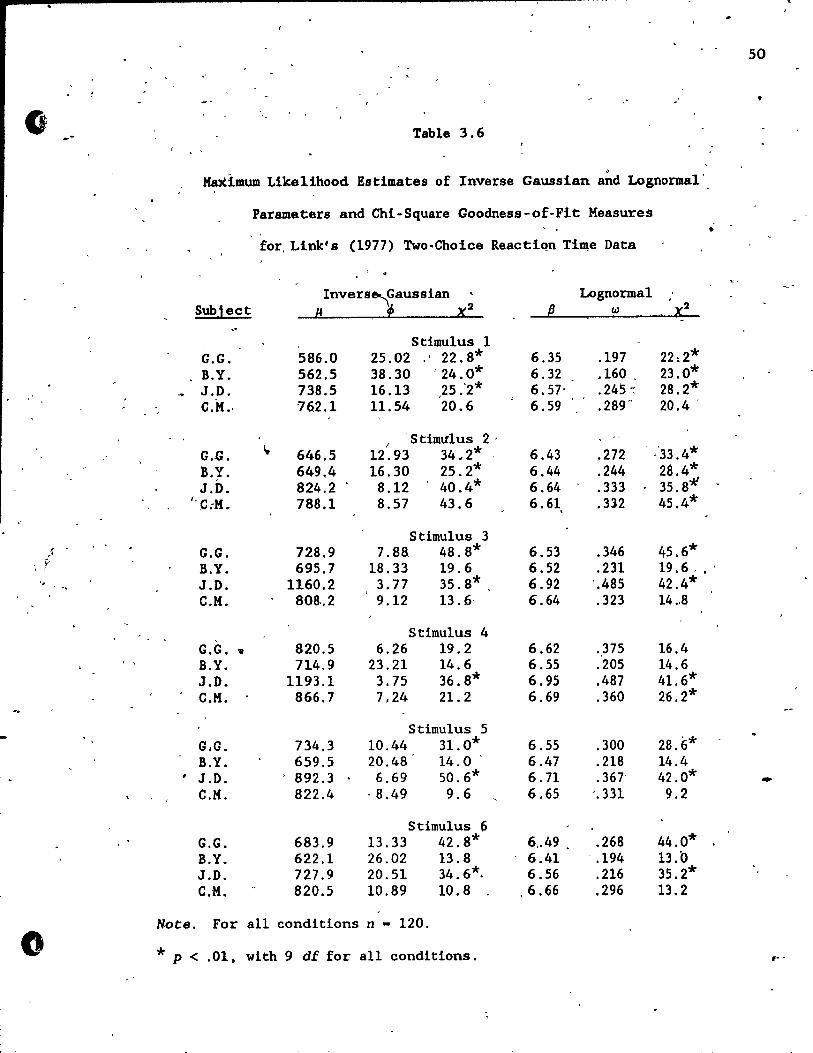
50
• .
0 Table 3.6 .--
,. K~imum Likelihood Estimates of Inverse Gaussian and Lognorma1'
Parameters and Chi-Square Goodness-of-Fit Heasures , . • , '
for, Link' s (1977) Two-Choice ReactiQn Ti~e Data
0
Invers~Gaussian ' Lognorma1 Sublect H f x 2 {J lA) , x2
Stimulus 1 G.G. 586.0 25.02 22.8* 6.35 .197 22~2* B.Y. 562.5 38.30 ' 24.0* 6.32 .160 _ 23.0*
-. J.O. 738.5 16.13 25:2* 6.57' .245 -: 28.2* C.H., 762.1 11.54 20.6 6.59 .289~ 20.4 -
{ 'Stimulus 2,
G.G. ... 646.5 12.93 34.2* 6.43 .272 - .'33.4* B.Y. 649.4 16.30 25.2* 6.44 .244 28.4* J.O. 824.2 8.12 40.4* 6.64 .333 35.8*'
" C;H~ 788.1 8.57 43.6 6.61 .332 45.4* ,
Stimulus 3 .... 1 G.G. 728.9 7.88 48.8* 6.53 .346 45.6*
- r-, , B.Y. 695.7 18.33 19.6 6.52 .231 19.6 , . ' '. J.O. 1160.2 3.77 35.8* 6.92 '.485 42.4*
C.H. 808,.2 9.12 13.6, 6.64 .323 14 .. 8
Stimulus 4 G.G •• 820.5 6.26 19.2 6.62 .375 16.4 B.Y. 714.9 23.21 14.6 6.55 .205 14.6 J.D. 1193.1 3.75 36.8* 6.95 .487 41.6* C.H. 866.7 7,24 21. 2 6.69 .360 2"6.2*
Stimulus 5 G.G. 734.3 10.44 31.0* 6.55 .300 28.6* B.Y. 659.5 20.48 14.0 ' 6.47 .218 14.4
• J.O. 892.3 6.69 50.6* 6.71 .367' 42.0* -C.K. 822.4 ,8.49 9.6 6.65 '.331 9.2
Stimulus 6 G.G. 683.9 13.33 42.8* 6,.49 . .268 44.0* B.Y. 622.1 26.02 13.8 6.41 - .194 13.0 J.O. 727.9 20.51 34.6*. 6.56 .216 35.2* C.ti. 820.5 10.89 10.8 .6.66 .296 13.2
Note. For a11 conditions n - 120.
0 * p < . 01, with 9 di for a11 conditions . ".-
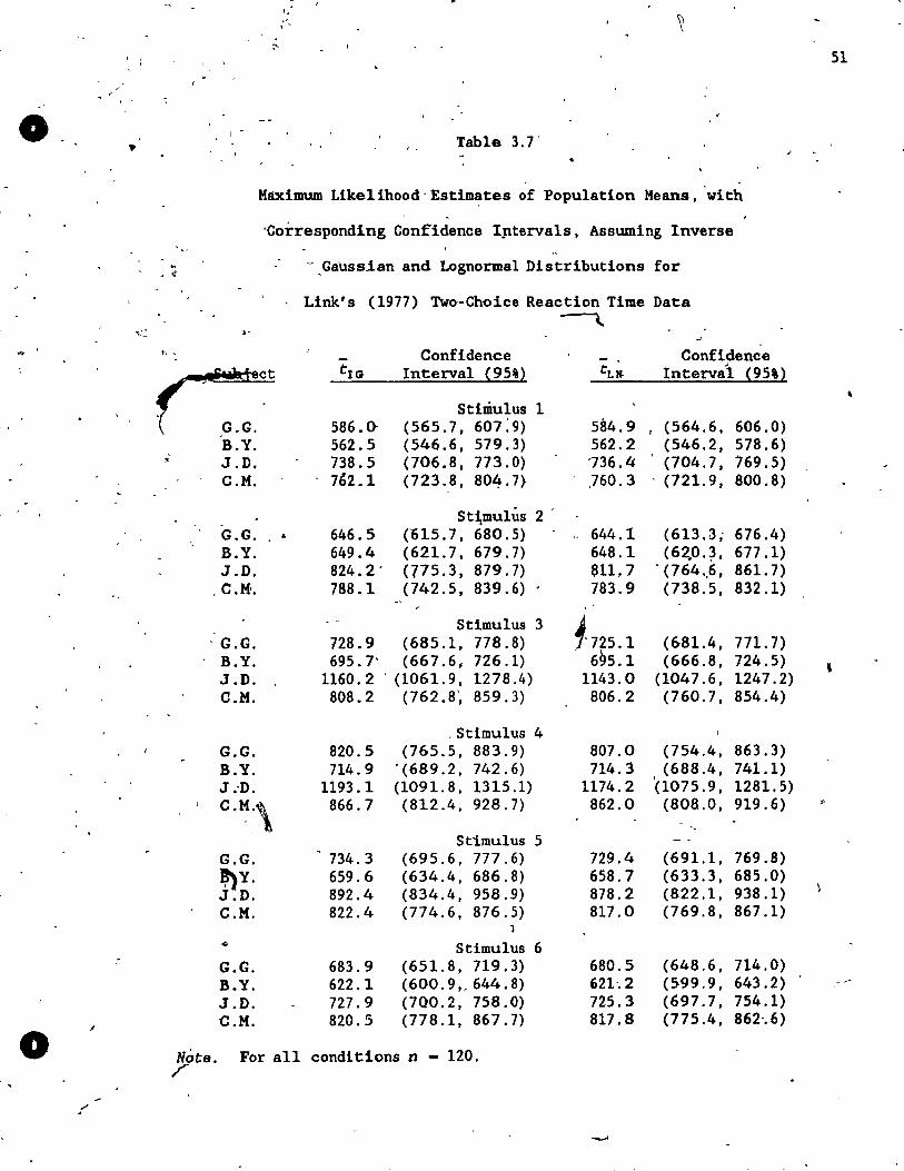
0
"
0
:"
.-
l ' 1
,.
",' ~
. ' . . ' ..
51
1 -
Table 3.1"
-Màximum Like1ihood" Estim~tes of Population Means. "with
'Corresponding Confidence Ipterva1s, Assuming Inverse "
~ - ,Ga'ussian and Lognorma1 Distributions for • <il
Link' s (1977) Two'-Choice Reaction Time Data ---... .' " , Confidence Confidence , - -
r: t IG Interva1 {95%} tLH- Interval {95'~ ,
. ,G.G. Stimulus 1
586.0- (565.7,607:9) 584.9 , (564.6, 606.0) B.Y. 562.5 (546.6, 579.3) 562.2 (546.2, 578.6)
. J.D • 738.5 (706.8, 773.0) '736.4 ' (704.7, 769.5) C.M. 7~2.1 (723.8, 804.7) ,760.3 ' (721.9, 800.8)
St~mu1üs 2 . ,
G.G. 646.5 (015.7, 680.5) 644.1 ( 613 . 3 ," 676.4 ) B.Y. 649.4 (621.7,679.7) 648.1 (62.0.~, 677 .1) J .D. 824.2' (775.3, 879.7) S11,7 '(764.,6, 861.7)
' C.M. 788.1 (742.5, 839.6) , 783.9 (738.5, 832.1)
Stimulus 3 ~'725.1 . G.G. 728.9 (685.1, 778.8) (681.4, 771.7) B.Y. 695.7' (667.6, 726.1) 695.1 (666.8, 724.5) J .D. 1160.2 ' (1061. 9, 1278.4) 1143.0 (1047.6, 1247.2) C.M. 808.2 (762.8', 859.3) 806.2 (760.7, 854.4)
,Stimulus 4 G.G. 820.5 (765.5, 883.9) 807.0 (754.4, 863.3) B.Y. 714.9 '(689.2, 742.6) 714.3 (688.4, 741.1)
1
J ."D. 1193.1 (1091.8, 1315.1) 1174.2 (1075.9, 1281. 5)
C.~~\ 866.7 (812.4, 928.7) 862.0 (808.0, 919.6)
Stimulus 5 G.G. 734.3 (695.6, 777.6) 729.4 (691.1, 769.8) !)Y. 659.6 (634.4, 686.8) 658.7 (633.3, 685.0) J .D. 892.4 (834.4, 958.9) 878.2 (822.1, 938.1) C.M. 822.4 (774.6, 876.5) 817.0 (769.8,867.1)
1 .. Stimulus 6 G.G. 683.9 (651.8, 719.3) 680.5 (648.6, 714.0) B.Y. 622.1 (600.9,,644.8) 621-.2 (599.9, 643.2) J.D. 727.9 (700.2,758.0) 725.3 (697.7, 754.1) C.M. 820.5 (778 . 1, 867. 7) 817.8 (775.4, 862".6)
Note. For a11 conditions n - 120. /'
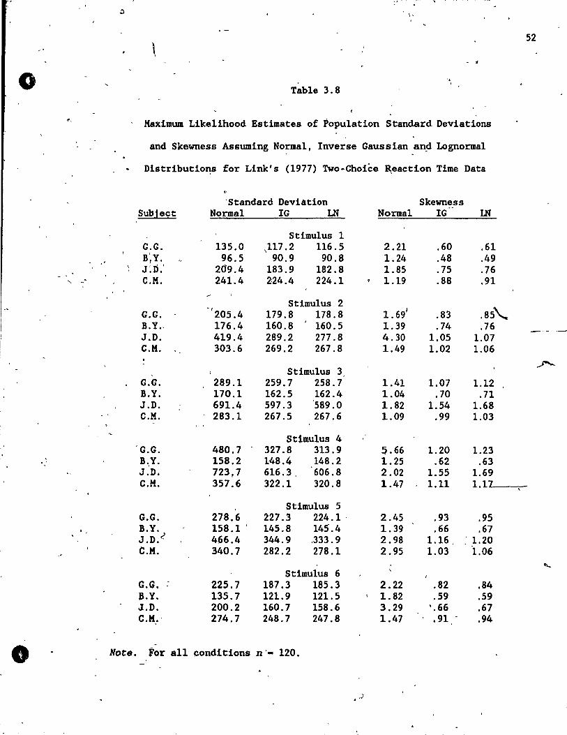
o
, t
o
discussed in chapters 4 and 5.
Random Walk Hodels
" ' In random wa1k mode1s the observer ls assumed to accumulate 1
information about a stimulus over time. In two-choice experiments it
i~ postu1ated that on1y one counter is used, but that it has two
criteria. This process can be vlewed as a random wa1k between postive
and negative criterion levels, or apsorbing barriers, rel~ted to the two
alternatives. If the evidence ta11ied exceeds one of these 1evels, the
corresponding alternative is chosen. Though there will be randomness
in the moment-to-moment count, it will tend to dr~ft towards the
correct criterion (Townsend & Ashby, 1983, chap. 10).
One of the first random walk models, proposed by Stone (1960), ls
based on the sequential probabi1ity ratio test procedure deve10ped by
1 ~ald (1947) and leads directly to the inverse Gaussian distribution.
Edwards (1965) and Laming (1968) have since expanded on this model.
Basically it assumes that an observer makes use of the availab1e
,information in an optimal fashion. To do 50 the movement of the random
walk is determined by calculated like1ihood ratios. These ratios
ref1ect ~he like1ihood,that some obtained input value was samp1ed from
the "distribution associated with one of the àlternatives. More
specifica11y, if a psychological value Xl is received, the observer's
• choice behaviour can be described using the statistlc
53
\
;:; - 1 ....
o
o
"
(3.1)
where fA ,and Es are the probability density functions associated with
the alternatives A and B, respective1y. If Y1 lies above the criterion
level for alternative A, then the response RA related to ehoosing
alternative A is made. Conversely, if the y 1 value fal1s below the
negatiye of the criterion level for alternative B then the respoRse RB
related to choosing alternative B is made. If neither criterion level
ls surpassed another sample Is taken and a second log likelihood Y2 is
computed and ad~ed to YI' The ab ove mentioned comparisons are then made ~
again. The position of the walk, denoted ,by w~ after k sm:ples have ,
been drawn and neither barrier has been crossed is then
l (3.2)
l'
Jl 'An improvement 'to Stone' s approach, cal1ed the' "relative judgment
'~eory (RJT) , was proposed by Link and Heath (1975). The observer in
this model is assumed to eonstruct a mental referent on a psychologieal
continuum as the first step in solving the discrimination problem .
• This referent, which is random and has an associated distribution, i8
" then utilized as a standard against whieh sampled stimulus values can'
be compared. In partieular, if xi ls à psychologieal stimulus, then
the theory assumes that the subject draws a sample XRj
from the
raferent distribution and co.putes the difference Yi '. Xi - XRj
' The
position of the random walk, denoted Wk as before, after k samp~es have
been drawn and neither barrier has been erossed is then
Q'
54
o
o
- l ~ ~j ---_. -r , ~'l~ " "Ii·· - ., J,
'; -...,. • ~ ~ ... ··of .- ... _. -.. ";." --.;-- ... ~ i ... .;. .. , r
__ (3.3)
Whi1e good modeling results have been achieved using the RJT theory,
its statistical applications are quite 1imited. On1y basie response
probabilities and'mean reaction time statistics May be determined usin&
RJT random walk models. > As the prime objective of this thesis is the'
development of general purpose statistical techniques for latency data,
other theories similar to the RJT model, which do no~ lend themselves
to statistical analyses, are not c~nsidered.
Hazard Functions f
The Most obvious way to describe a random variable, such as the
onset of a stimulus, is by its density or distribution function.
However, this may not be a natur~l approach from a subject's point of \,:)
view. The person who is waiti~ for the onset of a ~timulus has some
sense of the probability e~·t~curring in the next' instant of time.
This probabilïty may increase, decrease or stay,consta~t with time.
As an alternative to working with' the densÙY or di!ttribution . . function aione, one May renormalize the density by the probablli:y that
the event failed to occur prior to time e. The result is cailed Uha
hazard function. d -Denoting the densi~y of the rando~ variable by f(t)
and its distributi~n function by F(t), the hazard function i8 given by ,
~ .
55
,0
'. 1 •
..
..
'. ~
\
1
o ..
h(t) f(t) 1 - F( t) ,
(3.4) ,
J
. 'For a complete review of the basic properties of thls function, 1
l<a1bfl;elsch and Prentice (1980, ,chap. 1), Lawless (1982, chap'. 1),
and Luce (1986, chap. 1) may be consu1te~.
1 Psychologists working with the hazard 'function often calcula te the .. log survivor functioy{, which 1s log[l - 'F(t:)]. The relationship of this'
" function to the hazard functlon may be seen ~ way of the following
'derivation (Luce, 1986,'chap. 1):
h(t:) __ f(t) 1 - F(t)
dF(t)jdt -: 1 - F(t) ,,~
0.
\ '
- -d1og[1 - F( t)] dt (3.5)
'b
Actual data 'can be conveniently summarized by plotting the log ) . s~lv6r function against time' t,' since the negati:,ve of th~ slope of
( . the resulting gràph ls the haz~rd f~nction. Proceeding,further, note
that both 'sides of Equation 3.5 mey be integrated to yield the . , .
formula '.\
.. • F(t).'" 1 -f~p L -J: ~(l[)dll] '" \
. , ,Diffetentiation then ,produces the follo~ipg expression fpr the
densltf function: 0
• •
•
56
o
o
( (3.7)
• So by Equation 3.5 it is clear that the hazard funetion ean .be
completely defim!d by the denSity and distrib.ution functions, and
Equations 3.6 and 3.7 show that the density and distribution functions ..
~, can be determined separately (by the hazard ,function alone. This latter
feature makes the hazard function p~rticu1ar1y attractive to work with
sinee it, characterizes the response time distribution as completely as ,
does the characteristic fun'ction. Using this fact, estimates of the
hazard funetions may be used to ru1e out certain parametric families of
distributions while modeling reaetion times.
Burbeck and Luc,e (1982) studied the ha'zard functions associated ,
with simple reaction times to auditory s~im\,\1i. They found that l1azard
functions associated with weak tones,were monotone increasing and
peaked for stronger ones. They then examined the theoretical hazard
functions corresponding to well-known distributions. On1y Grice's
random criterion mode1 (1968, 1972) and the inverse Gaussian possessed
a~tributes which accounted for the genera1 qualitative shape of the
peaked hazard function. Figures 3.3 and 3.4 contain plots of inverse
Gaussian hazard function surfaces, with p - 1 and ~ varying, from two
different views.
57
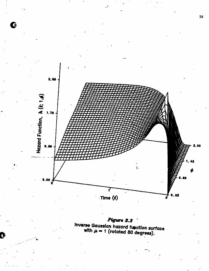
, 1
o
1
1."
o "
'.
,l1rne Ct)
l'igure 8.8 ~
Inverse Gausslan hazard 1U11ctfon surface wHh JI. III 1 (rotated 80 degrees).
,
58
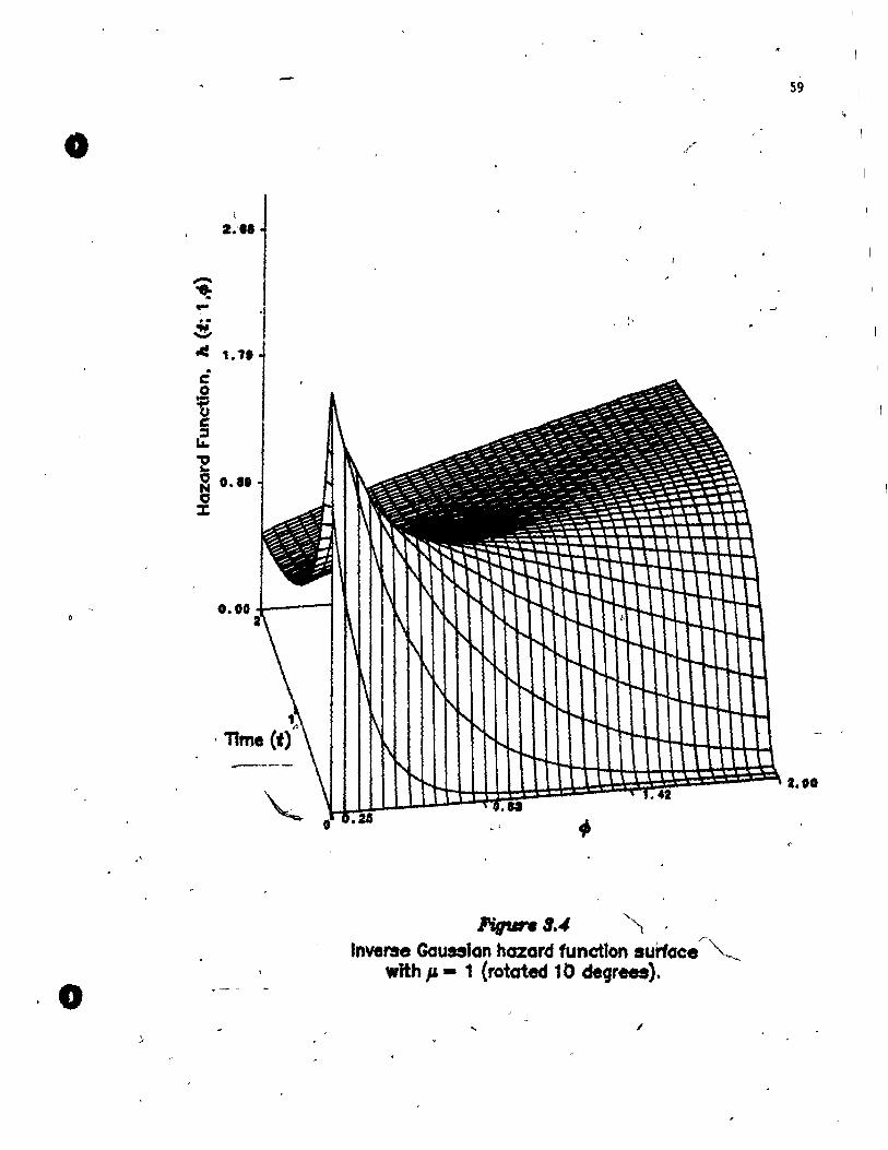
S9
o ,1
(
2.'"
,.... -e: ... .4; :' "'" toC! 1.11 . C 0 ~ (J c .: "2 :3 O." 0 :t
0.00 -'----,
.,.--...---
Pigure 8.4 "" Inverse Geu.ton hozard functton sUrloce
r
,,--
wlth JI - 1 (rotated 10 de9rees). -
·0 '. /
-----------:-----.-----.--............. ...---,..----;-----------;;-" ---~_ .. _-----
. ,
o
"
, Convolutlons
As outlined'ln chapter 1; psychologists a~e often interested in l ,
breaklng'reactlon times down into two parts corresponding to the
decision and residual times. Of course, researchers are usually only
interested in the decision latencies. Hence, given total reaction ,
tlmes, which are aIl that ar~ available to an experimenter, the goal is
then to eliminate the nuisance times (i.e., the residual latencies) in
order to be leT,.-~n the distribution of the decision latency.
In chapte it was also mentioned that psychologists usually
assume that the (total. decision and residual) may be
treated as random variables and that the latter two are independent.
To fix notation, let the total, decision and residual latencies be
denoted by T, D and R, respectively. The distribution functions of the
three random variables will be l,abelled aS FT' FD' and FR ~nd it will
be assumed that their corresponding densities IT' ID' and IR exist.
Now if D is fixed to some value x. where 0 < x < t, t being the . observed time, then R must equal the value t - x. Then the probability
of the event (T ::s t) may be broken down, using the assumption of
independence of D'and R, as follows (Luce, 1986, chap.1):
ft:
FT(t) - P(D - x, R St-x) dx o
t: f P(D-x)P(RS t-x) dx o
t: - f ID(X)FR( t-x) dx o
. '
\
(3.8)
60
o
,
. "
The derlsity ET is then obtained by differentiaÙng the above
equation ~ith respect to t. That Is,
(3.9)
, R May be fixed at some y, with D - t - y, to obt~in the,
and
..
expressions in Equations 3.9 and 3.11 are both known as
convolutions of the densities ED and fR' respe~tivè1y. Thë
cor~esponding characteristic functions satisfy the re1ationship
•• " ,j ,
(3.10)
(3.11')
(3.12)
Using this equ~;ion a study of the structure of reaction times May be
undertaktn by way. of a Fourier analysis (Christ,ie & Luce, 1956; Green,
1971). A simi1ar multiplicative form is a1so true 'of the corresponding
moment-generating function. "
The resu1ts given i~ this section are used in chapter 5 to
convolute two inverse Gaussian distributions. t'
61
o
!
f
:Chapter 4
The Shifted In~rse Gaussian Distribution
Shlftlng the!> Or1~ln
In every experimental situation a minimum latent period is
implicitly present. Even when simple tasks are given, the lower
\ \\
response bound can be appreciable and shbu1d be taken ~nto account-if
the data are to be adequately modeled. Besides goodness-of-fit
considerations, estimates of an added shift parameter can provide
investigators with some additional insight into the processes which
result in a particular latency. In some cases experimenters may wish
to subtract out individual estimated shift parameters bèfore performing
statistical analyses.
There are a number of three-paramet~r generalizations of two-
parameter distributions which are applicable to skewed data. The three
most common are the lognormal (Cohen, 1951; Hill, 1963; Harter & Moore,
1966), the g8mma (Harter & Moore, 1965; Cohen & Norgaard, 1977), and
the Weibull (Harter & Moore, 1965; Dubey, 1966; Rockette, Antle &
K1imko, 1974). In aIl of these cases obtaining maximum 1ikelihood
estimates can be difficult. In particular t~ere are paths in the ~
parame ter spaces which yield the minimum observed value as the
estimated shift parameter.
A well-behaved alternative is the shifted inverse Gaussian which
62
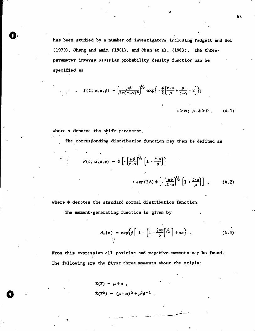
.. 63
has been studied by a number of investigators inc1uding Padgett and Wei . ,
(1979), Cheng a~d Amin (1981), and Chan et al. (1983). The three-
parameter inverse Gaussian probabi1ity density function can be
specified as
t> ct; p, ~ > 0' , (4.1)
where CI denotes the shife parameter. - . The cor~esponding distribution function may then be defined as
(4.2)
where ~ denotes the standard normal distribution function.
The moment-generating function is given by
<4.3)
From this expression a11 positive and negative moments may be found.
The fo11owing are the first three moments about the origin:
E(T) - JJ + a ,
o É(T2) - (p + a) 2 + p2~-1 ,
<--~- - _.-:--..
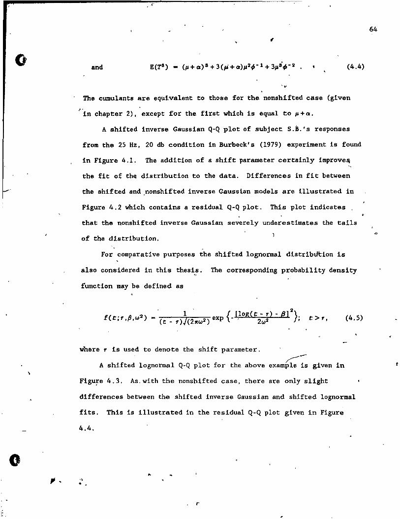
o
\
o
"
and (4.4)
The cumulants are equ1valent to those for the nonshifted case (glven
~'1n chapter 2), except for the f1rst which ls equal to p + Q.
A shifted inverse Gauss ian Q-Q plot of subj ect S. B. ' s responses
from the 25 Hz, 20 db condition in Burbeck's (1979) experiment is found
in Figure 4.1. The addition of a shift parameter certain1y improve!i
the fit of the distribution to the data. Differences in fit between
the shifted and.nonshifted inverse Gaussian models are illustrated in
Figure 4.2 which contains a residual Q-Q plot. This plot indicates .
that the nonshifted inverse Gaussian severe1y underestimates the tails
of the distribution.
-For comparative purposes the shifted lognormal distrib~ion is
a1so considered in this thesis. The corresponding probability density
functlon may be defined as
, 2 f(t,'r, R,(2 ) _ l exp { [log(t: - r) - Pl }.
~ (t - r)J(21fw2 ) - 1 2w2 , t:>r, (4.5)
where r is used to denote the shift parameter.
~~'--A shifted 10gnormal Q-Q plot for the above example ls given in
Figure 4.3. As.with the nonshifted case, there are only slight
differences between the shifted inverse Gaussian and shifted lognormal
fits. This is i11ustrated in the residual Q-Q plot given in Figure
4.4.
. \ . . ...
1"
64
o
,
"
o
,..... " CI) en E ...... en CI)
E o-
f-
C' .0
+'
" 0 CI)
, et:
- "
· 2500
\ ; '/ - .~ .....
2000
... ".'
15'0
,
1000 -
~ 500 \
f ,)
o~ ______ ~ ______ ~ ______ ~~ ______ ~ ______ ~ o 500 ,1000 1500 2000 .
Shlfted Inverse Gausslan Quant Iles (msec)
J'igure 4. f
2500
Shlfted lnverse Gousslan Q-Q plot of 413 redctlon tlmes obtalned from sub ject 5.8. durlng the 250 Hz, 20 db conditIon of
Burbeck's (1979) simple reactlon tlme experlment.
65
--'.
/'
-' ' ;' 1
t
l'igure 4.R Shifted minus nonshlfted Inve'" Gausslan Q-Q plot of 413 reactton
tlmes obtalned from subJecl S.B. durlng the 250 Hz. 20 db condition of Burbeck's (1979) sImple reactlon ttme experiment. '
, -
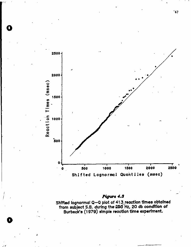
o
o
- ~ "
2500
2000 ' . ...... (,) CI) 0)
E ""' 1500 0)
CI) E .. . -t-~_C
0 .-...., (,)
c CI)
0:::
1000
e
.. 500
O~ ______________ ~ ______ ~ ________ -------r - 0 500 1000 1500 2000 2500
Shi fted Lognormal Quant Iles (msec)
l'igun 4.3 5hlfted lognormdl Q-Q plot of 413 react10n t1mes obta1ned
from subject 5.8. during th~Zt 20 db cond1tlon of Burbeck's (1979) simple reactlon tlme experlment.
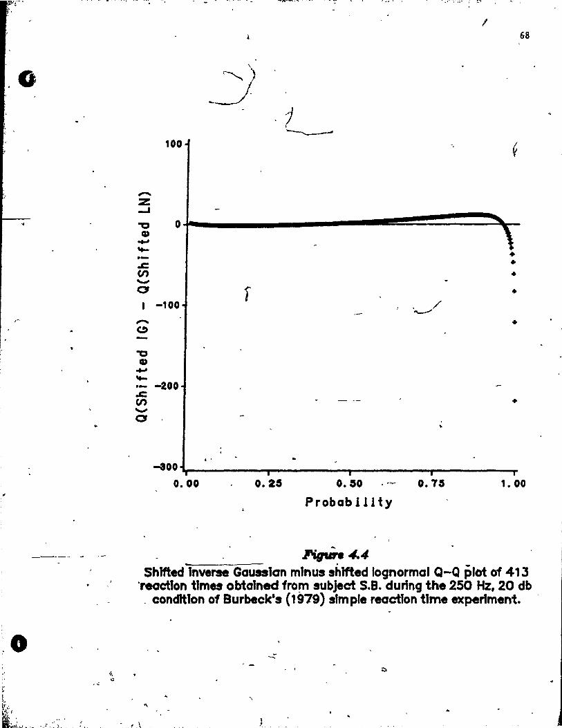
o
" .
';
,-
:0 "
. .' • 1 ..... __ ~ ,*.~ .",) .
1 68
100 "
" :z ..... -0 0
CD eotJ ~ - • .&:! • en • '"" 0 r • 1 -100 1 ............. /
" • (!) --0 CD
eotJ ~ .- -200 .&:! (1) • '"" 0 ..
. ' ~oo.-________ ~ ________ ~ ________ ~ ________ ~
0.00 O. 2S O. SO ' ....- O. 7 S 1.00
Probab 111 ty
l'igtir. 4.4 Shlfted "Inverse Gausslan mInus shlfted lognormal Q-Q plot of 413
'reacllon tlmes obtalned fro~ subject S.8. during the 250 Hz, 20 db . conditIon of Burbeck's (1979) sIm pie reactlon tlme experlment. '
. - ~ .\
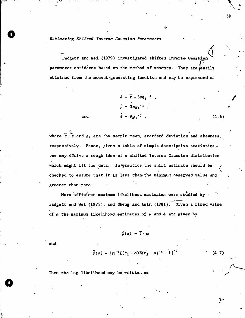
. .,,~ .~ -
"
0
o
: '" .... .. ~ ~ .. . " : t • ; .,
~
Estlmatlng Shifted Inverse Gaussisn Parameters
o ()
Padgett and Wei (1979) investigated shifted inversa Gauss~
parameter esti~àtes based on the method of moments. They are feasi1y
obtained from the moment-generating function and may be expressed as
" ë - 3sg1 -1
ct -
1\ 3sg1
-1 }J - ,
" and· ~ - 9g1 - 2 ;, (4.6)
_.~
where t, sand gl are the samp1e mean, standard deviation and skewness,
respectively. Hence, given a table of simple descriptive statistics,
one may,derive a ~ough idea of a shlfted lnverse Gaussian distribution
which might fit the data. In~ractice the shift estimate should be .. ( checked to ensure that lt is 1ess than,the minimum observed value and
greater than zero.
More 'efficient maximum like1ihood estimates were st~died by .
---Padgett and Wei (~979), and Cheng and Amin (1981). Given,. fixed value
of Q the maximum 1ike1ihood estimates of p and ~ are given by
~(a) - t - Q
and
Then the log likelihood may be written·as
. -
(4.7)
,-\" .. . \
~ . 69
./ r
•
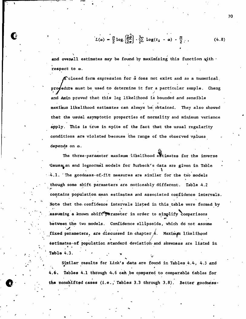
o· \"
."
f •
• f
. , .
... '\.
"
, , .. } .
··,·n (~J 3~ L(Q) - '2 10g, 211' • ï'L. log(tj - a) !!
2 " , (4.8)
\ , 1
and ovel".ollii estimates May be found by maxim1zing this function J(.ith .
respect to a.
, ~closed form expression for a does not exist and so a numerical,
~riedure must be used to determine it for.} particular sample. Cheng
and Amin proved that this log likelihood is bounded and sensible
maximum likelihood estimates can always b~obtained. They also showed
that the usdal asymptotic properties of normality and minimum variance
apply. This i9 true in spite of the fact that the usual regularity
c9nditions are violated because the range of the observed v~lues
depen~B on cr.
The three-parameter maximum 'likelihood ~imates for the inverse
'Gausl\an and lognormâl models for Burbeck' s data are given in Table \
,4.1. ' The goodness-o(-fit measures are similar for the two modela
thQugh some shift parameters are noticeably different. Table 4.2 \.y" ,
contains population mean estimates and associated confidence intervals. . "
Note that the, confidence intervals listed "
;assuming , a ..known sh'if~rameOter in order
in this,table were formed,by , ta simplify comparisons
, ~'f" , \
bètween the two models. Confidence ellipsoids, which dd not assume 'J ,
, ,fixed pa~ameters.' are dlscus'sed in Chapter). MaximtfD likèlihood
éstimates--,of pop~14tion standard deviatiot and skewness are listed in ~ .
Table 4.3. ,. S~milar results for Link's data are found in Tables ,4.4, 4.5 and .. . J.
4.6. Tabl-es 4.1 through 4.,6 c'3tt ,be cpmparerl; to comparablè tables for j
the nonsliift~d cases (Le. " Tables 3.3 through 3.8). Better goodness-
'"
70
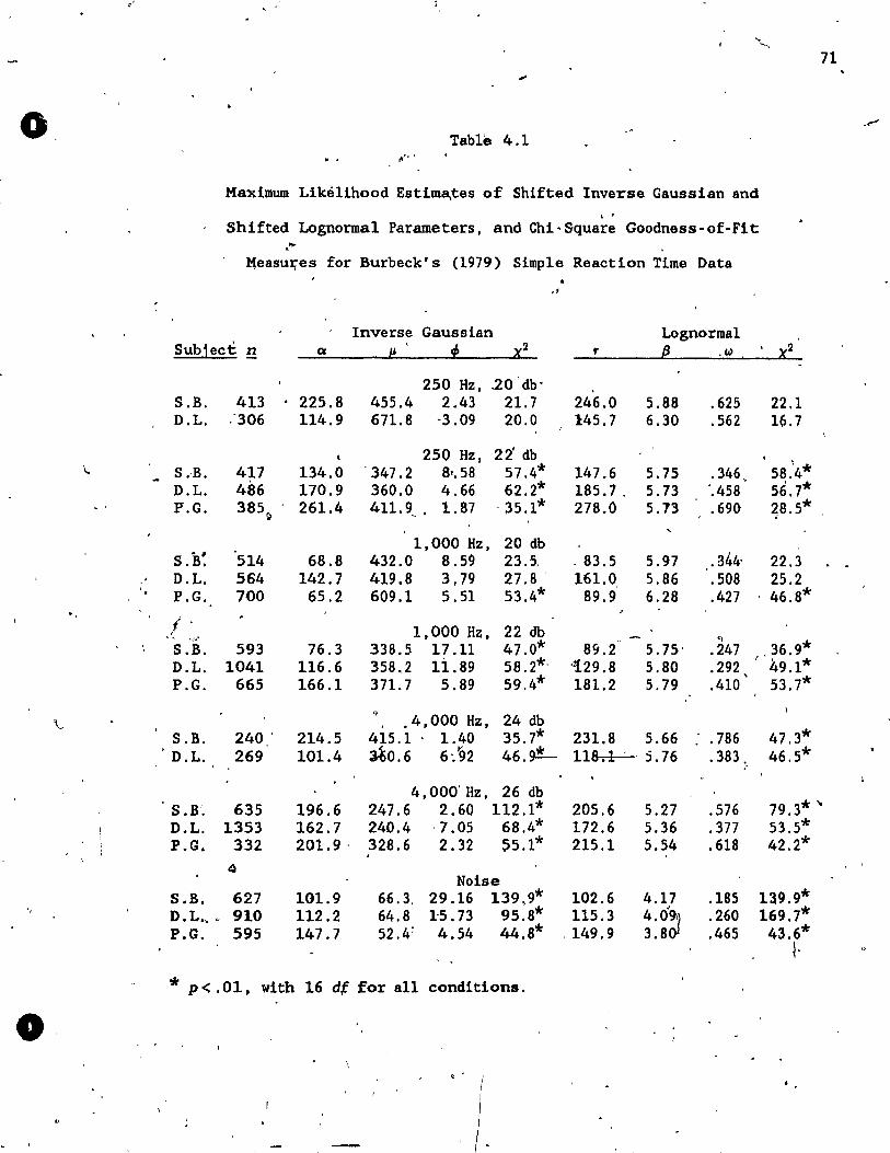
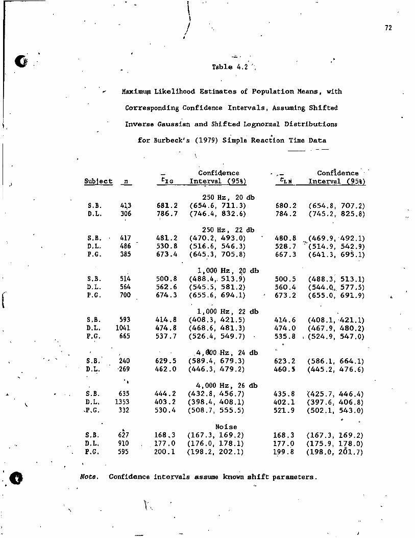
\ , / 72
;
Table 4.2 ~."
, Maximupl Likelihood Estimates of Population Means. with
Corresponding Confidence Interva1s, Assuming Shifted
Inverse Gaussian and Shifted Lognormal Distributions
". . for Burbeck' s (1979) Simple Reaction Time Data
- Confidence .- "Confidence' . "
.; Sublect .1!... t IG Int~rva1 (95%) tut Interval (95%)
250 Hz, 20 db S.B. 4p 681.2 (654.6, 711.3) 680.2 (654.8, 707.2) D.L. 306 786.7 (746.4, 832.6) 784.2 (745.2, 825.8)
250 Hz, 22 db S.B. 417 481.2 (470.2, 493.0) 480.8 .. ..<469.9. '492.1) D.L. 486 530.8 (516.6, 546.3) 528.7 '(514.9, 542.9) P.G. 385 673.4 (645 .. 3, 705.8) 667.3 (64l. 3, 695.1)
1 ,000 Hz, ~O db , S.B. 514 500.8 (488.4,. 513.9) 500.5 (488.3, 513.1) D.L. 564 562.6 (545.5, 581.,2) 560.4 (544.0, .. 577.5)
r P.G. 700 674.3 (655.6, 694.1) 673.2 (655.0, 69l.9) .s.
1 ,000 Hz, 22 db S.B. 593 414.8 (408.3, 421. 5) 414.6 (408.1, -421.1) D.L. 1041 474.8 (468.6, 481. 3) 474.0 (461.9, 480.2) P.G. 665 537.7 (526.4, 549.7) 535.8 • (524.9, 547.0)
A, 000 .Hz, 24 db S.B. 240 629.5 (589.4, 679.3) 623.2 (586.1, 664.1) D.L. '269 462.0 (446.3, 479.2) 46Q.S (445.2, 476.6)
, . 4,000 Hz, 26 db
Jo . . - S.B. 635 444.2 (432.8, 456.7) 435.8 '(425.7,446.4)
" D.L. 1353 403.2 (398.4, 408.1) 402.1 (397.6,406.8)
.P.G. 332 530.4 (508.7, 555.5) 521..9 (502.1, 543.0)
.. Noise S.B. '627 168.3 (167.3, 169.2) 168.3 (167.3, 169.2) D.L. 910 177.0 (176.0, 178.1) 177.p (175.9, 178.0) P.G. 595 200.1 (198.2,202.1) 199.8 (198.0,201.7)
,10 Note. Confidence intenrals assume known shift parameters. .
\ \ ".
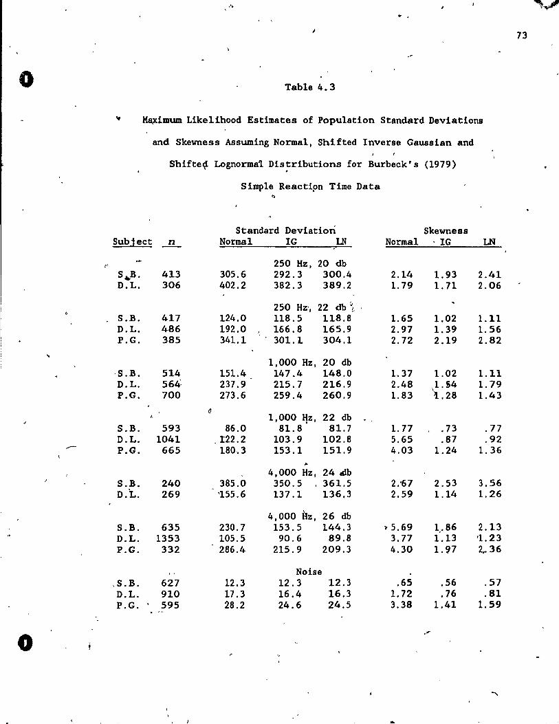
,'. ~ " .
1 73
..-'
0 Table 4.3
Ma..ximum Like 1 ihood Estimates of Population Standard Deviations
and Skewness Assuming Normal, Shifted Inverse Caus si an and
Shifte~ Lognorma'l. Dis ;ributions for Burbeck' s (1979)
Simple Reactipn Time Data ..
Standard Deviation Skewness Sub1ect n Normal IG LN Normal . IG LN
," 250 Hz, 20 db S~B. 413 305.6 292.3 300.4 2.14 1.93 2.41 D.L. 306 402.2 382.3 389.2 1. 79 1. 71 2.06
250 Hz', 22 db~, S.B. 417 124.0 118.5 118.8 1.65 1.02 1.11 D.L. 486 192.0 166.8 165.9 2.97 1. 39 1. 56 P.C. 385 341.1 301.1 304.1 2.72 2.19 2.82
, 1,000 Hz, 20 db
-S .B. 514 151.4 147.4 148.0 1. 37 1.02 1.11 D.L. 564~ 237.9 215.7 216.9 2.48 {.54 l. 79 P.C. 700 273.6 259.4 260.9 1.83 .28 1.43
a 1,000 IJz, 22 db . ,
S.B. 593 86.0 81. 8 81.7 1. 77 .73 .77 D.L. 1041 1:22.2 103.9 102.8 5.65 .87 .92
,.-- P.C. 665 180·.3 153.1 151.9 4.03 1.24 1. 36 ,.
4,000 Hz, 24 .ob S.B. 240 385.0 350.5 361.5 2:67 2.53 3.56 D.L. 269 '155.6 137.1 136.3 2.59 1.14 1.26
4,000 Hz, 26 db S.B. 635 230.7 153.5 144.3 '1' 5.69 1,.86 2.13 D.L. 1353 105.5 90.6 89.8 3.77 1.13 '1.23 P.C. 332 286.4 215.9 209.3 4.30 1.97 2 .. 36
Noise ,S.B. 627 12.3 12.3 12.3 .65 .56 .57 D.L. 910 17.3 16.4 16.3 1. 72 .76 .81 P.C. 595 28.2 24.6 24.5 3.38 1.41 1.59
0 .'"
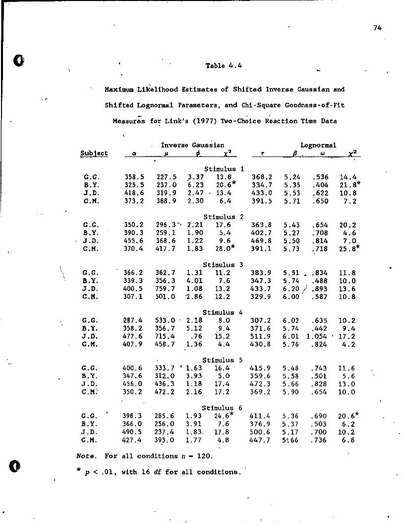
74
0 Table 4.4
L
Maximum Likel1hood Estimates of Shifted Inverse Gaussian and - ,.
Shifted Lognorma1 Parameters, and Chi-Square Goodness-of-Fit .- , 1
Measures fo~ Link's (1977) Two-Choice Reaction Time Data
Inverse Gaussian Lognormal Subject a IJ f x2 ., {J . W x2
Stimulus 1 G.G. 358.5 227.5 3.37 13.8 368.2 5.24 .536 14.4 B.Y. 325.5 237.0 6.23 20.6* 334.7 5.35 .404 21.8* J.D. 418.6 319.9 2.47 13.4 433.0 5.53 .622 10.8 a.M. 373.2 388.9 2.30 6.4 391.5 5.71 .650 7.2
Stimulus 2 G.G. 350.2 296.3-' 2.21 17.6 363.8 5.43 .654 20.2 B.Y. 390.3 259.1 1.90 5.4 402.7 5.27 .708 4.6 J.D. 455.6 368.6 1.22 9.6 469.8 5.50 .814 7.0 C.M. 370.4 417.7 1.83 28.0* 391.1 5.73 .718 25.8*
\ Stimulus 3 •
G.G. 366.2 362.7 1.31 11.2 383.9 5.51 .. .834 11.8 B.Y. 339.3 356.3 4.01 7.6 347.3 5.74 .488 10.0 J.O. 400.5 759.7 1.08 13.2 433.7 6.20 / .893 13.6 C.M. 307.1 501.0 '2.86 12.2 329.9 6.00
, .587 10.8
Stimulus 4 G.G. 287.4 533.0 . 2.18 8.0 307.2 6.02 .635 10.2 B.Y. 358.2 356.7 5.12 9.4 371.6 5.74 .442 9.4 J.D. 477 .6 715.4 .76 15.2 511.9 6.01 1.054 17.2 C.M. 407.9 458.7 1.36 4.4 430.8 5.76 .824 4.2
Stimulus 5 .. , G.G. 400.6 333.7 ( 1.63 16.4 415.9 5.48 .743 11.6 B.Y. 347.6 312.0 3.93 5.0 359.6 5.58 .501 5.6 J .D. 456.0 436.3 1.18 17.4 472.3 5.66 .828 13.0 C.M: 350.2 472.2 2.16 17 .2 369.2 5.90 .654 10.0
Stimulus 6 G.G. 398.3 285.6 1. 93 24.6* 411.4 5.36 .690 20.6* B.Y. 366.0 256.0 3.91 7.6 376.9 5.37 .503 6.2 J .D. 490.5 237.4 1. 83, 17.8 500.6 5.17 .700 10.2 C.M. 427.4 393.0 1. 77 4.8 447.7 5°.66 .736 6.8 .
NoCe. For all conditions n - 120.
0 * P < .01. with 16 dl for a11 conditions.
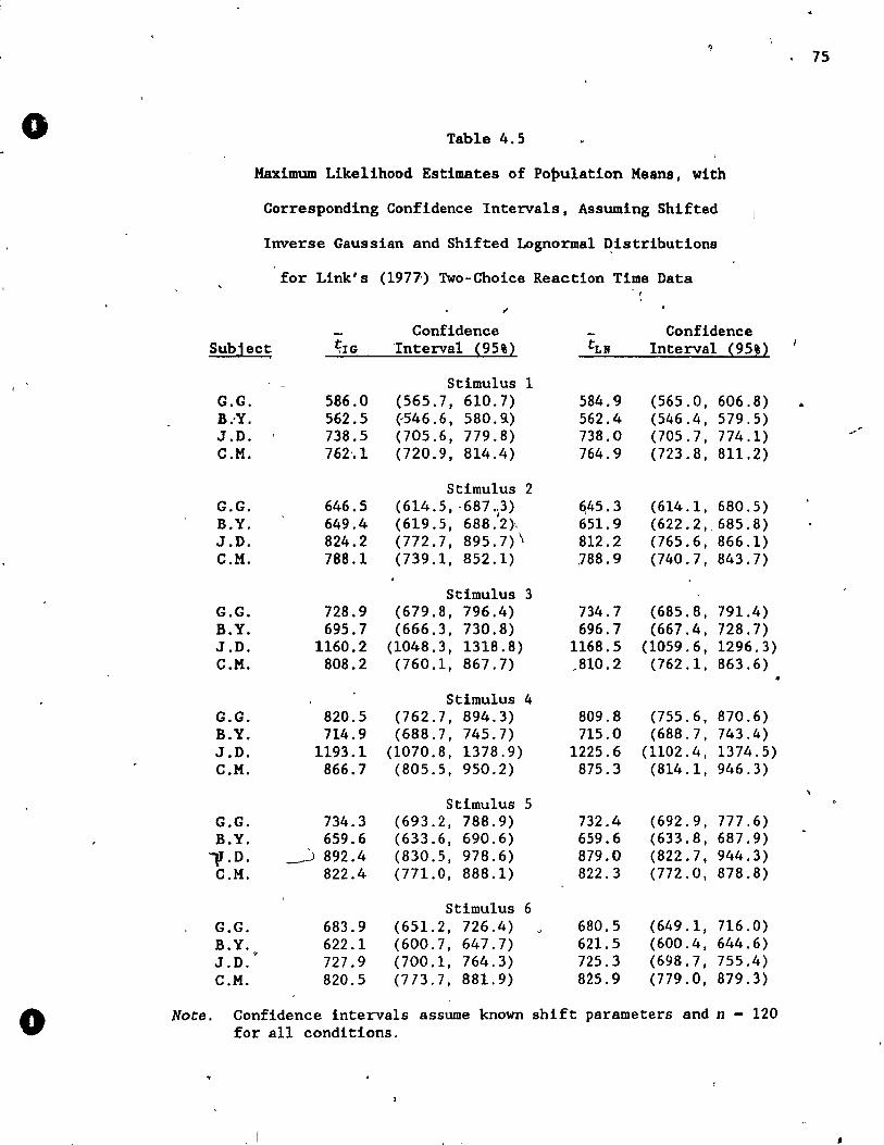
, 75
0 Table 4.5
Maximum Like1ihood Estimates of Po~u1ation Means, with
Corresponding Confidence Interva1s. Assuming Shifted
Inverse Gaussian and Shifted Lognorma1 ~istributions
for Link' s (1977') Two-Choice Reaction Time Data
.. - Confidence - Confidence
Subject t:IG 'Interva1 (95%) t LN Interval (95%)
Stimulus 1 G.G. 586.0 (565.7,610.7) 584.9 (565.0, 606.8) .. B .. Y. 562.5 (-546.6, 580.9.) 562.4 (546.4, 579.5) -J.D. 738.5 (705.6, 779.8) 738.0 (705.7, 774.1) .'
C.M. 762'.1 (720.9, 814.4) 764.9 (723.8, 811. 2)
Stimulus 2 G.G. 646.5 (614.5, ,687,,3) 6,45.3 (614.1,680.5) , B.Y. 649.4 (619.5,688.2)\ 651. 9 (622.2,,685.8) J.D. 824.2 (772.7, 895.7) \ 812.2 (765.6, 866.1) C.M. 788.1 (739.1, 852.1) ,788.9 (740.7, 843.7)
Stimulus 3 G.G. 728.9 (679.8, 796.4) 734.7 (685.8, 791.4) B.Y. 695.7 (666.3, 730.8) 696.7 (667.4, 728.7) J.D. 1160.2 (1048.3, 1318.8) 1168.5 (1059.6, 1296.3) C.M. 808.2 (760.1,867.7) ,810.2 (762.1, 863.6)
Stimulus 4 G.G. 820.5 (762.7, 894.3) 809.8 (755.6, 870.6) B.Y. 714.9 (688.7,745.7) 715.0 (688.7, 743.4) J.D. 1193.1 (1070.8, 1378.9) 1225.6 (1102.4, 1374.5) C.M. 866.7 (805.5, 950.2) 875.3 (814.1, 946.3)
Stimulus 5 G.G. 734.3 (693.2, 788.9) 732.4 (692.9, 777 .6) B.Y. 659.6 (633.6, 690.6) 659.6 (633.8, 687.9) l' .D. ~ 892.4 (830.5, 978.6) 879.0 (822.7, 944.3) C.M. 822.4 (771.0, 888.1) 822.3 (772.0, 878.8)
Stimulus 6 G.G. 683.9 (651.2, 726.4) 680.5 (649.1, 716.0) B.Y. 622.1 (600.7, 647.7) 621.5 (600.4, 644.6) J.D. 727.9 (700.1, 764.3) 725.3 (698.7, 755.4) C.M. 820.5 (773.7,881.9) 825.9 (779.0, 879.3)
0 Note. Confidence intervals assume known shift parameters and n - 120 for a11 conditions .
. 1 •
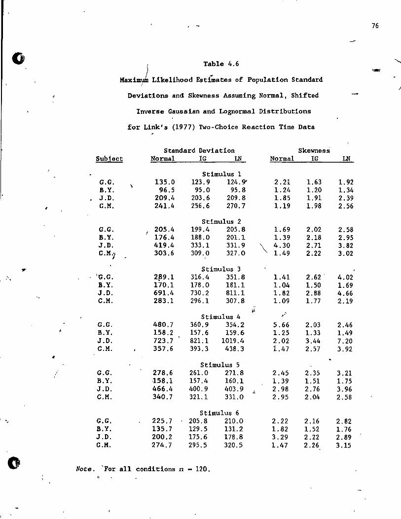
. - 76
0 mol Table 4.6 "-~
Maxi Like1ihood Esti~ates of Population Standard 1 )
Deviations and Skewness Assuming Normal, Shifted
Inverse Gaussian and Lognorma1 Distributions
for Link's (1977) Two-Choice Reaction Time Data
Standard Deviation Skewness Subject Normal lG LN Normal lG LN
Stimulus 1 G.G. 135.0 123.9 124.9' 2.n 1.63 1. 92 B.Y. 96.5 95.0 95.8 1.24 1.20 1.34 . J.D . 209.4 203.6 209.8 1. 85 1.91 2.39
, C.M. 241.4 256.6 270.7 1.19 1.98 2.56
Stimulus 2 G.G.
J 205.4 199.4 205.8 1.69 2.02 2.58
B.Y. 176.4 188.0 201.1 1.39 2.18 2.95 J.D. 419.4 333.1 331. 9 \ 4.30 2.71 3.82 C.M:i 303.6 309.0 327.0 1.49 2.22 3.02
li!' Stimulus 3 ~ 'G.G. 2p9.1 316.4 351.8 1.41 2.62 . 4.02 , ,
B.Y. 170.1 178.0 181.1 1.04 1.50 1.69 J.O. 691.4 730.2 811.1 1.82 2.88 4.66 C.M. 283.1 296.1 307.8 1.09 1.77 2.19
" )\
~
Stimulus 4 ,,' G.G. 480.7 360.9 354.2 5.66 2.03 2.46
j. B.Y. 158.2 157.6 159.6 1. 25 1.33 1.49 J.D. 723.7 821.1 1019.4 2.02 3.44 7.20 C.M. 357.6 393.3 438.3 1.47 2.57 3.92
" Stimulus 5 1
1
G.G. 278.6 261.0 271.8 2.45 2.35 3.21 1
B.Y. -158.1 157.4 160.1 1.39 1.51 1. 75 J.D. 466.4 400.9 403.9 fl 2.98 2.76 3.96 C.M. 340.7 321.1 331.0 2.95 2.04 2.58
Stimulus 6 . , G.G . 225.7 205.8 210.0 2.22 2.16 2.82 B.Y. 135.7 129.5 131.2 1.82 1.52 1. 76 J.D. 200.2 175.6 178.8 3.29 2.22 2.89 C.M. 274.7 295.5 320.5 1.47 2.26 3.15
0 Note. 'For aIl conditions n - 120. 0
o
..
o
~
of-fit measures are evident for the shifted distributibns, especial"ly
for Link' s data. Estimates of population standard deviation and
skeWI].ess are appreciably improve~ with the three-parameter models.
This suggests that the confidence intervals for the population mean are ",,-;
underestime.ted when nonshifted models are assumed. -,-
f
Shifted and Censored Inverse Gausslsn DistrLbut:1.on ,
In order to fit latency data well a model must not only account
for the foreperiod of nonresponse but also the possibility of censoring
which cornrnonly occurs in psychology experiments. As mentioned in
chapter 1 only Type l censoring, in whlch one preset upper time liml t
is" set for a11 trials wl thin a particular condition, 15 cons idered in
this thesis.
Following the usual approach ta determining a likelihood in 'a
censoring situation (Kalbfleisch & Prentice, 1980,_ chap. 3; Lawless,
1982, chap. 1), assume that the random time variables T j 1 sare
independent identically distributed inver:;e Gaussian. The upper bound
on responding will be denoted b~ c and sô Tl is only observable if , ...
Ti:Sc. Now let Ii be the indicator of the event [T1!!Oc]. Then the data
~ can be represented by the n pairs of random variables (S1,I j ) where
Si -min(Ti,c) ,
(4.9)
77
,1 1
o
"
• 1
-• That~18, Si 18 equa1 to Ti 1f 1t is observed, and to C otherwisé, w1th
,11. 1nd1cat1ng whether T1. has been c~nsored or not.
The jo1nt probab11ity function 0f Si and Ii 1s
(4.10)
• • For a samp1e of n times and 1ett1ng m denote the number of observed
n times (i.e. 1 ~1. - m) 1 the log 1ikelihood function 1s g1ven by ..,
where'
and
L - ~ log (~) - ~ r Ii log (s1. - a)
.!~ (Si- a p ) - L Ii -- + -- - 2 + (n-m)1og[l - F(e») 2 JS si - a
. Z 2 - - (/ .. tP a]% (1
.J
c - a) +--JS
(4.11)
(4.12)
(4.13)
The first partial derivat1ves with respect to the parameters are
,.
nom 2(c - a) [1 _ F(e») [Z2g(Zl) + ZI exp(24))g(Z2) ]
l,
(4.14)
78
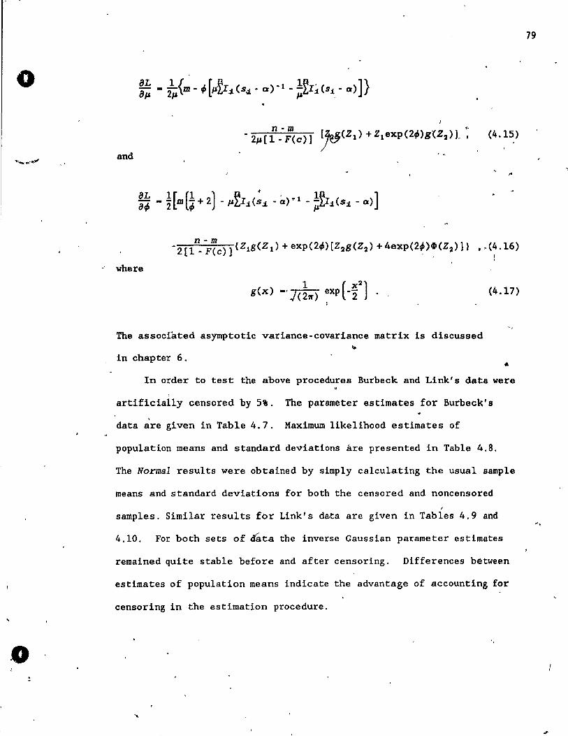
79
o
(4.15)
and ,.
where
(4.17)
The associated asymptotic variance-covariance matrix is discussed
in chapter 6.
In order to test the above procedures Burbeck and Link's data were ,
artificially censored by 5%. The parameter estimates for Burbeck's ,
data are given in Table 4.7. Maximum 1ikelihood estimates of
population means and standard deviations are presented in Table 4.8.
The Normal results were obtained by simply ca1cu1ating the usual sample
means and standard deviations for both the censored and noncensored
"
samples. Similar results for Link's data are given in Tables 4.9 and "',
4.10. For both sets of dâta the inverse Gaussian parameter estimates
remained quite stable before and after censoring. Differences bétween
estimates of population means indicate the advantage of accounting for
censoring in the estimation procedure.
"
.0
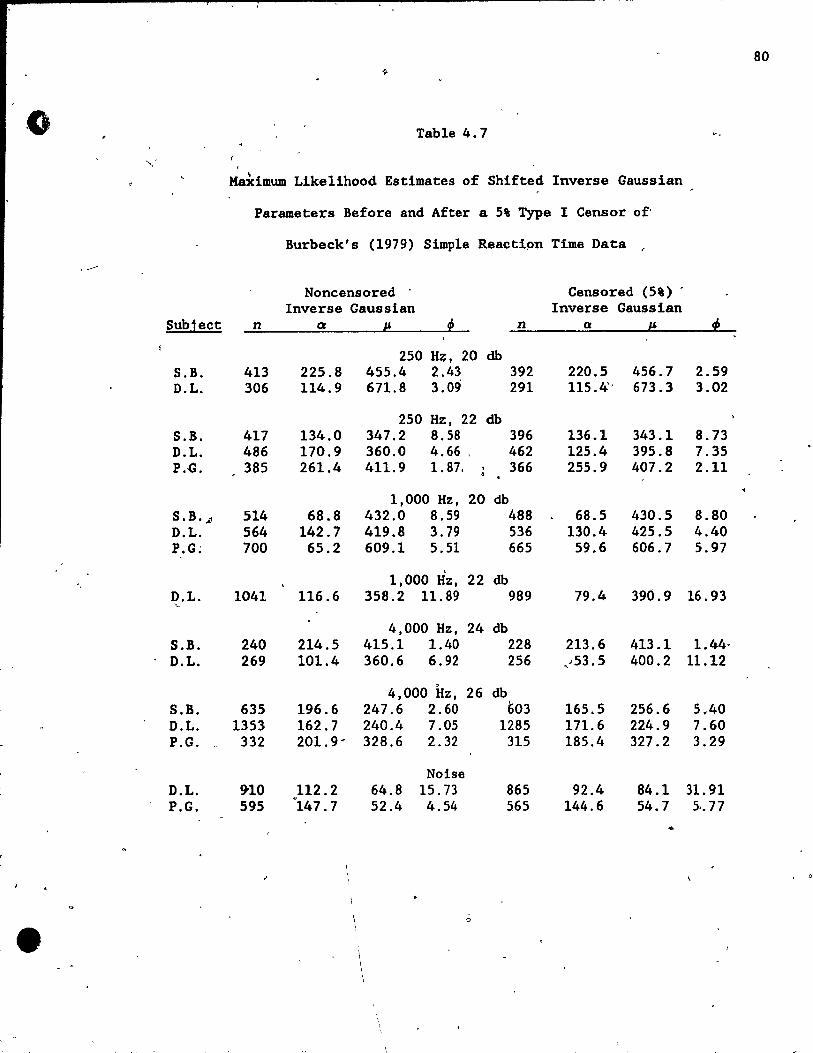
80
" Table 4.7 ., "'-- ,
~imum Like1ihood Estimates of Shifted Inverse Gaussian
Parameters Before and After a 5% Type 1 Cens or of'
Burbeck's (1979) Simple Reactipn Time Data ,
, ---Noncensored Censored (5%) ,
Inverse Gaussian Inverse Gaussian Sublect n ct JJ ; n a JJ ;
250 H~, 20 db S.B. 413 225.8 455.4 2.43 392 220.5 456.7 2.59 D.L. 306 114.9 671.8 3.09 291 115.4" 673.3 3.02
250 Hz, 22 db S.B. 417 134.0 347.2 8.58 396 136.1 343.1 8.73 D.L. 486 170.9 360.0 4.66 , 462 125.4 395.8 7.35 P . .a. 385 26l.4 411.9 1.87. 366 255.9 407.2 2.11
1,000 Hz, 20 db S.B.,6) 514 68.8 432.0 8.59 488 68.5 430.5 8.80 D.L. 564 142.7 419.8 3.79 536 l30.4 425.5 4.40 P.G; 700 65.2 609.1 5.51 665 59.6 606.7 5.97
1,000 Hz, 22 db D.L. 1041 116.6 358.2 11.89 989 79.4 390.9 16.93
4,000 Hz, 24 db S.B. 240 214.5 415.1 1.40 228 213.6 413.1 l.44· D.L. 269 101.4 360.6 6.92 256 ,~53. 5 400.2 11.12
4,000 Hz, 26 db S.B. 635 196.6 247.6 2.60 603 165.5 256.6 5.40 D.L. 1353 162.7 240.4 7.05 1285 171.6 224.9 7.60 P.G. 332 201.9~ 328.6 2.32 315 185.4 327.2 3.29
Noise D.L. 9-10 112.2 64.8 15.73 865 92.4 84.1 3l. 91
~
P.G. 595 147.7 52.4 4.54 565 144.6 54.7 S'.77 •
, 0
o
\
\
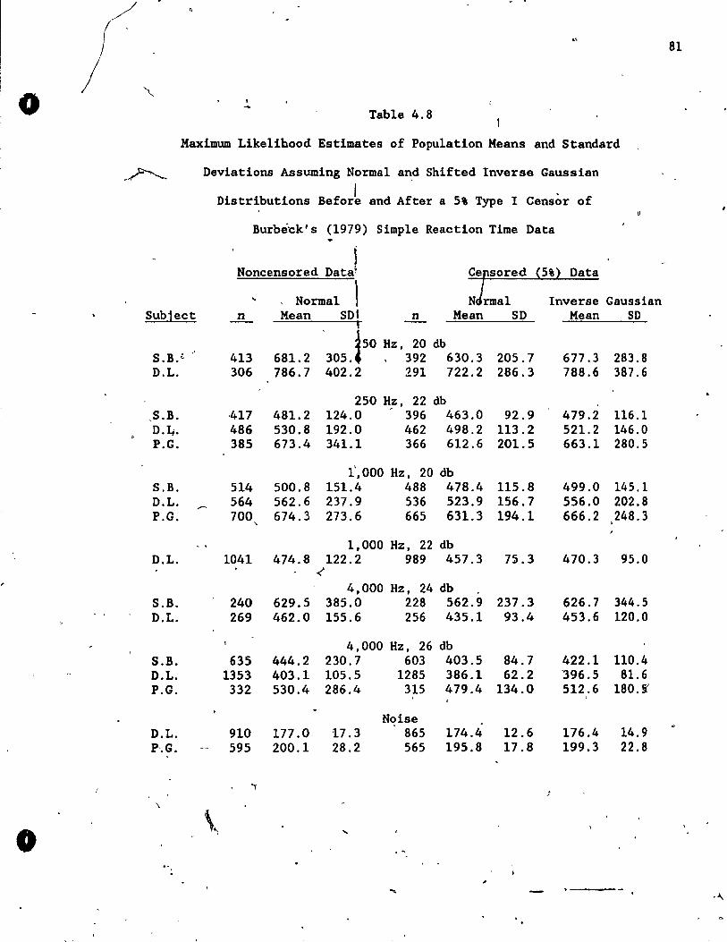
o •
81
o Table 4.8
Maximum Likelihood Estimates of Population Means and Standard
Deviations Assuming Normal a~d Shifted Inverse Gaussian j
Distributions Before and After a 5% Type 1 Censôr of
Burbe~k's (1979) Simple Reaction Time Data
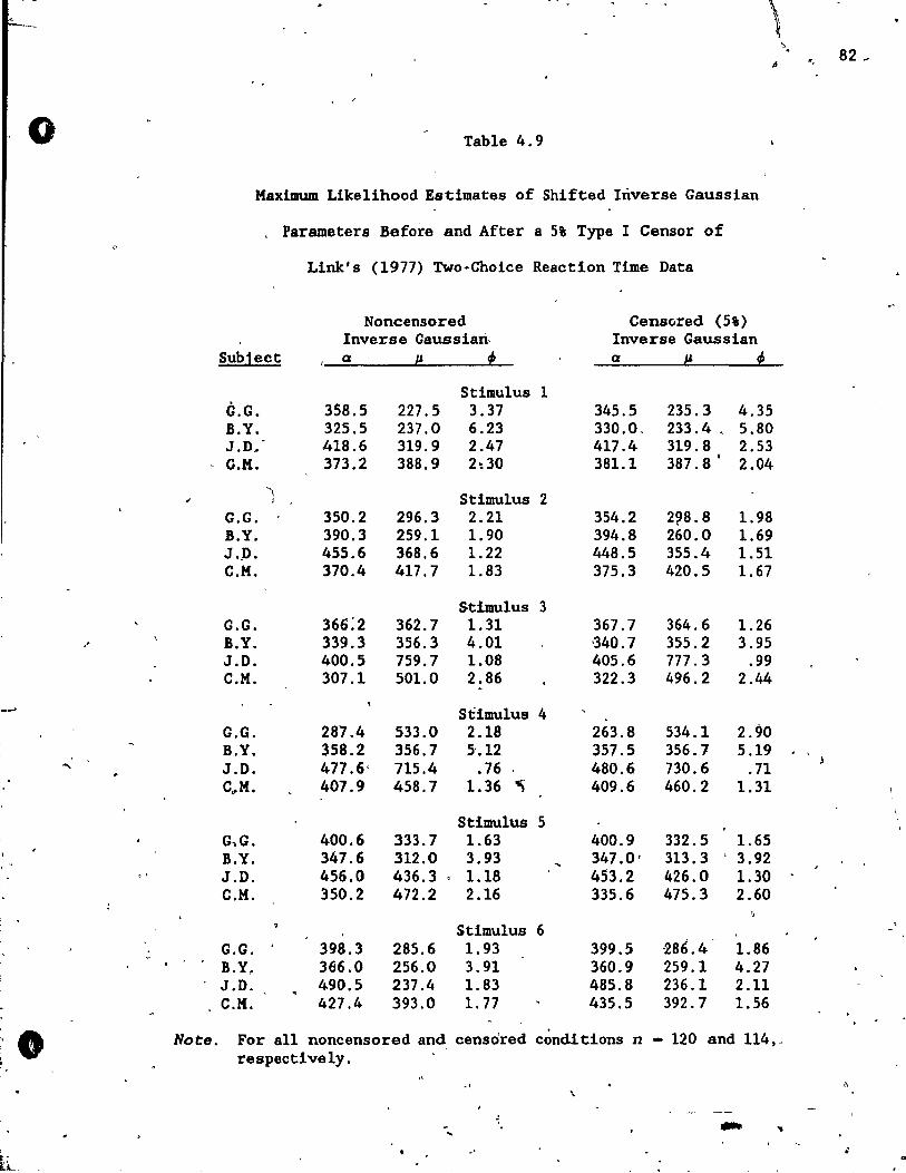
\ ~
.,~ 82 _
" "
/
0 Table 4.9
Maximum Like1ihood Estimates of Shifted Inverse Gaussian
, Parameters Before and After a 5% Type 1 Censor of
Link's (1977) Two-Choice Reaction Time Data
Noncensored Censc.red (5%) Inverse Gaussiari, Inverse Gaussian
Sublect Q p ; Q JJ ;
Stimulus 1 G.G. 358.5 227.5 3.37 345.5 235.3 4.35 B.Y. 325.5 237.0 6.23 330.0. 233.4 , 5.80 J .D~· 418.6 319.9 2.47 417.4 319.8 2.53
- O.M. 373.2 388.9 2~30 381.1 387.8' 2.04
" , 1 Stimulus 2 G.G. 350.2 296.3 2.21 354.2 2?8.8 1.98 B.Y. 390.3 259.1 1.90 394.8 260.0 1.69 J .. D. 455.6 368.6 1.22 448.5 355.4 1.51 C.M. 370.4 417.7 1.83 375.3 420.5 1.67
Stimulus 3 G.G. 366:2 362.7 1.31 367.7 364.6 1.26 B.Y. 339.3 356.3 4.01 '340.7 355.2 3.95 J.D. 400.5 759.7 1.08 405.6 777.3 .99 C.M. 307.1 501.0 2.86 322.3 496.2 2.44
--' Stimulus 4 G.G. 287.4 533.0 2.18 263.8 534.1 2.90 B.Y. 358.2 356.7 5'.12 357.5 356.7 5.19
"' J.D. 477.6' 715.4 .76 480.6 730.6 .71 C.,K. 407.9 458.7 1.36 'Ii\ 409.6 460.2 1.31
Stimulus 5 GoG. 400.6 333.7 1.63 400.9 332.5 1.65 B.Y. 347.6 312.0 3.93 347.0' 313.3 3.92
, ' J.D. 456.0 436.3 1.18 453.2 426.0 1.30 C.M. 350.2 472.2 2.16 335.6 475.3 2.60
Stimulus 6 286.4
-
G.G. . 398.3 285.6 1. 93 399.5 1.86 ,.
B.Y. 366.0 256.0 3.91 360.9 259.1 4.27 J.D. 490.5 237.4 1.83 485.8 236.1 2.11 C.M. 427.4 393.0 1.77 435.5 392.7 1.56
, • Not:e. For a11 noncensored and censored c~nditions n - 120 and 114, 0
respective1y. 1\
'\
-.. ... .. 1 • ti_
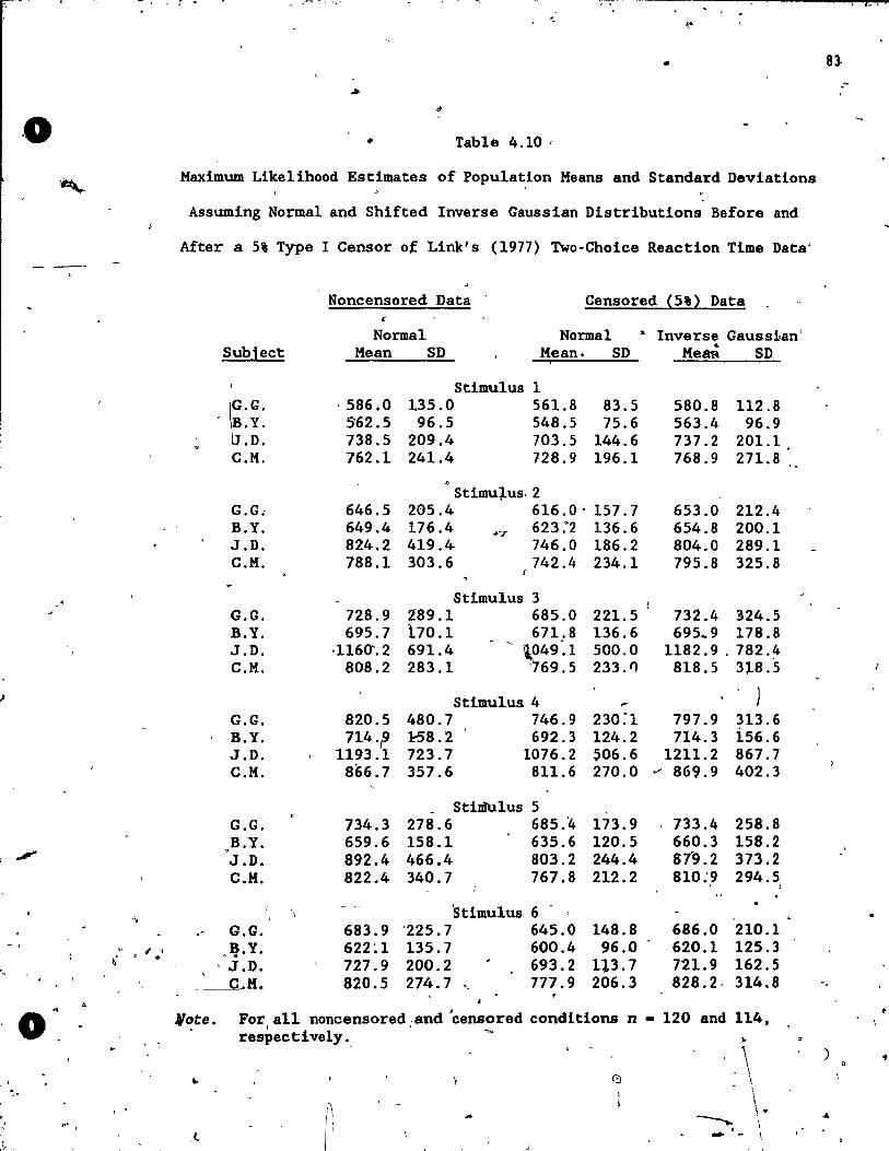
" ~ :- ... - ~..('., - ., -r~ ~ ..... --.--_ ... _-
1 ... >.-
~-<"-
.. n
"'* .-
~
·0 • Table 4.10 '
, Maximum Likelihood Estimates of Populat,ion Means and Standard Deviations . . Assuming Normal and Shifted Inverse Gaussian Distributions Before and
After a 5% Type l Censor of Link' s (1977) Two-Choice Reaction Time Data' - --
Noncensored Data Censored ~5'~ Data &
Normal Normal " Inverse Gaussian' Sublec't Mean SD Mean. SD MeaR SD
t
Stimulus 1 , ·586.0 135.0 561.8 83.5 ~.G. 580.8 112.8
B.Y. S62.5 96.5 548.5 75.6 563.4 96.9 .D. 738.5 209.4 703.5 144.6 737.2 201.1
C.M. 762.1 241.4 728.9 196.1 768.9 271.8 <>
StimuJ-us. 2 G.G, 646.5 265.4 616.0' 157.7 653.0 212.4 B.Y. 649.4 176.4 "-r 623.°2 136.6 654.8 200.1 J.O. 824.2 419.4 746.0 186.2 804.0 289.1 C.M. 788.1 303.6 742.4 234.1 795.8 325.8
,1 Stimulus 3 G.G. 728.9 2:89.1 685.0 221.5 732.4 324.5 B.Y. 695.7 170.1 671.8 136.6 695 .. 9 178.8 . -. J.O. ,1160'.2 691.4 \049.1 500.0 1182.9 , 782.4 C.M. 808.2 283.1 '169.5 233.1) 818.5 3).8. '5
) Stimulus. 4 } ... G.G. 820.5 480.7 746.9 230:1 797.9 313.6 B.Y. 714·fJ 1:-58.2 692.3 124.2 714.3 i56.6 J .D. 1193.1 723.7 1076.2 ~06.6 1211. 2 867.7 C.M. 866.7 357.6 811.6 270.0 ,Y 869.9 402.3
Stim'\1lus 5 G.G. 734.3 278.6 685.'4 173.9 733.4 258.8 B.Y. 659.6 158.1 635.6 120.5 660.3 158.2
.". ,
466.4 803.2 244.4 67'9.2 373.2 J.D. 892.4 C.K. 822.4 340.7 767.8 212.2 810:9 294.5 , ,
... '\ 'stimulus 6 -" G.G. 683.9 '225.7 645.0 148.8 686.0 210.1
" II' • )~.Y. 622~1 135.7 600.4 96.0 620.1 125.3 ~. < ..
, J.O. 727.9 200.2 693.2 1l3.7 721.9 162.5 " ,
_~K. 820.5 274.7 '. 777.9 206.3 828.2, 314.8
" " 0 Ilote. For aIl noncensored,and censored conditions n - 120 and 114, respectively " .~ :-..
~\ ) of
b
" ~ . .' \
\ . . . .. --... \ . .. ," " t i
,t.. - - \ ;".
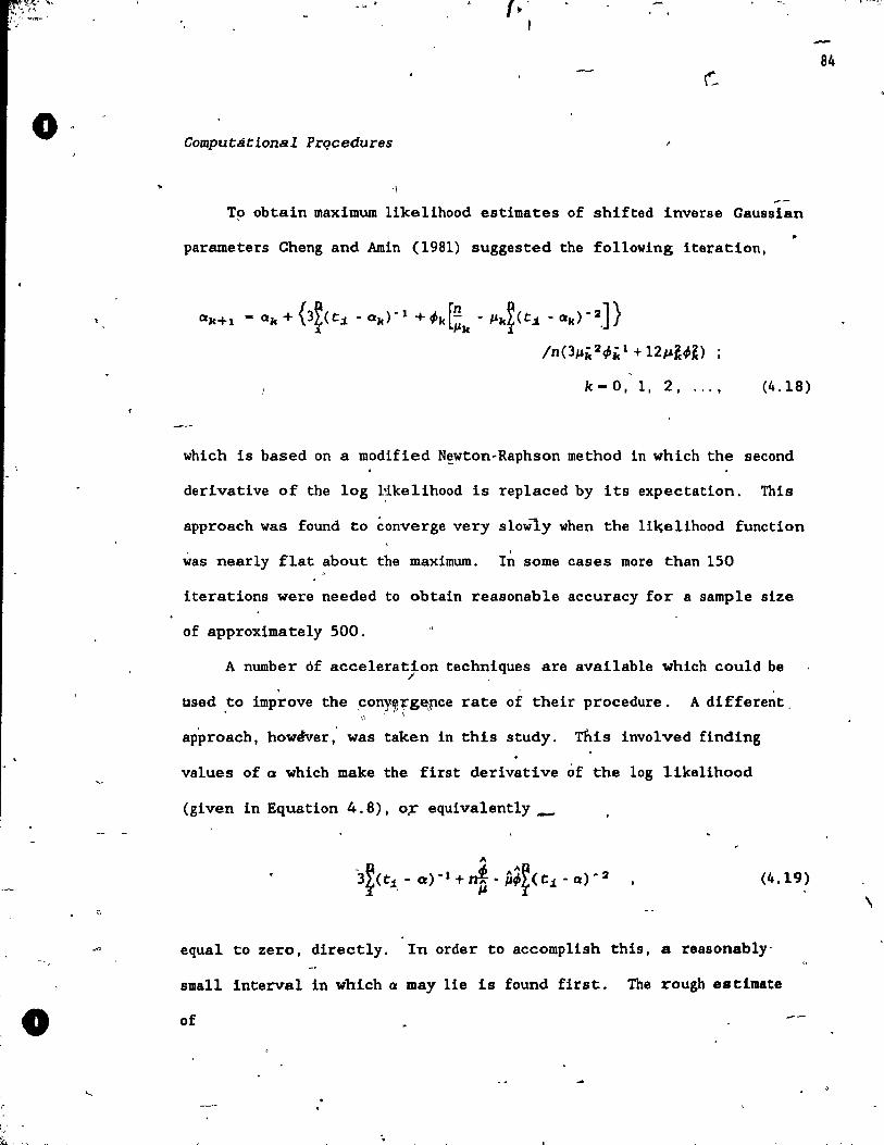
'Il .. ~~· ,,< t,j, ~-' .
o
o
.. w ." -f· ' t
-- "" """ "--"" T ~----'':-
84
Computàtional PrQcedures
'\
To obtain maximum likelihood estimates of shifted inverse Gaussian
parameters Cheng and Amin (1981) suggested the fol1owing Iteration,
0k+ 1 - Ok + {3 ~ ( t i - ok) - 1 + ~k [;k - JJk~ ( t i - Ok) - 2] }
/n(3JJic 2q,ic 1 + 121'~~~)
k-O, l, 2, ... , (4.18)
which is based on a modified N~wton-Raphson method in which the second
derivative of the log H.ke1ihood is replaced by its expectation. This
. approach was found to converge very slowÏy when the lUçelihood function
was nearly fIat about the maximum. ,
In some cases more than 150
iterations were needed to obtain reasonab1e accuracy for a sample size
of approximately 500.
A number of acce1eration techniques are avai1able which could be / .
, tlsed to improve the ,con)'i~~g~rce rate of their procedure. A different
• \\ L \ \
approach, howdver,' was taken in this study. This invo1 ved finding
values of ° which make the first derivative of the log Iikelihood
(given in Equation 4.8), o~ equivalently _
1\
3~(tj, - a) -1 + nt -P~~(tj - 0)-2 (4.19)
\
equai to zero, dlrectly. In order to accomplish this, a reasonably-
smaii Interval in wbich Q May lie 18 found first. The rough estlmate
of
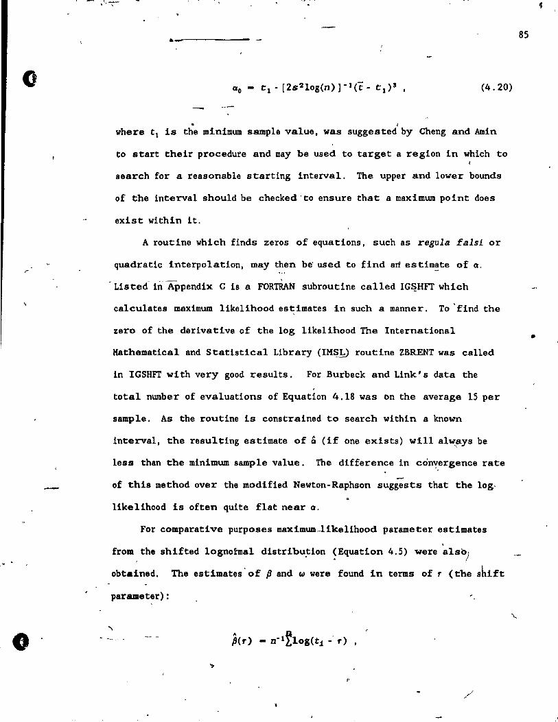
"1 - •
a--~----~=-85
o (4.20)
. , where t 1 is the minimum sample value, was suggested by Cheng and Amin
to start their procedure and may be used to target a region in which to
search for a reasonable s tarting interval. The upper and lower bounds
of the interval should be checked 'to ensure that a maximum point does
exist within it.
A routine which finds zeros of equations, such as regula fais! or
quadratic interpolation, may then be' used to find art estimate of Q,
Listed in Appendix C is a FORTRAN subroutine called IG~HFT which
calculates maximum likelihood estimates in such a manner. To' find the
zero of the derivative of the log likelihood The International • Hathematical and Statistical Library (IM~ routine ZBRENT was called
in IGSHFT with very good results. For Burbeck and Link' s data the ,
total number of evaluations of Equation 4.18 was on the average 15 per
sample. As the routine is constrained to search within a known
Interval, the resulting estimate of & (if one exists) will always be ,
less than the minimum sample value. The difference in cdn,:,,~rgence rate
of this method over the modified Newton-Raphson suggests that the log-
likelihood is often qulte fIat near a.
For comparative purposes maximum..1ikelihood parame ter estimates ,
frolll, the shifted lognofmal distribu.tion ~ Equation 4.5) were also;
obtained. The estimates -of fJ and w were found in terms of r (the shift
parameter) :
o /'
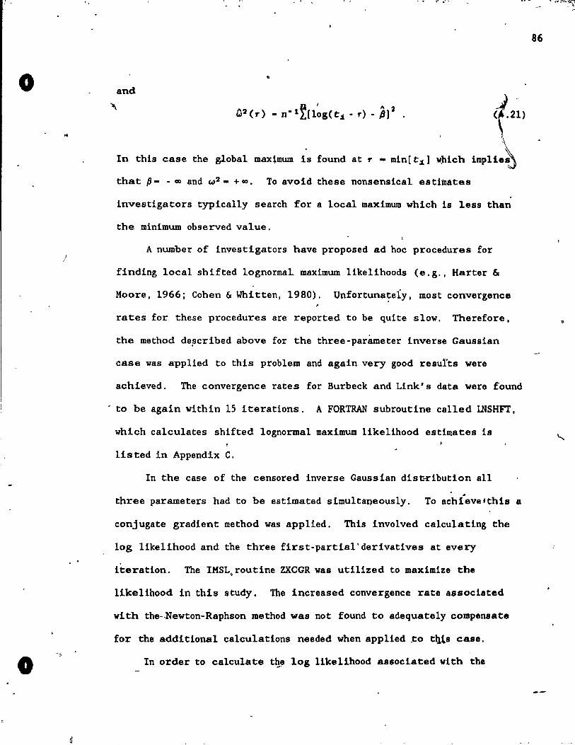
..... ,- ... ..,~ . ..;\-.,:: ...
86
o and
" P' "2 ",2(1') - n- 1L[10g(t,1· r) - P1 .
In this case the global maximum is found at l' - min[ 1:1 ] wJlich
that {J - - GO and ",2 - + GO. To avoid these nonsensical estimates
investigators typica11y search for a local maximum which is Iess than
the minimum observed value.
/ A number of investigators have proposed ad hoc procedures for
finding local shifted lognormal. maximum likelihoods (e. g., Harter &
Moore, 1966; Cohen & Whi tten, 1980). Unfortuna~eiy. most convergence
rates for these procedures are reported to be quite slow. Therefore.
the method depcribed above for the three -par8meter inverse Gaussian
case was applied to this prob1em and again very good resutts were
achieved. The convergence rates for Burbeck and Link' s data were found
to be again within 15 iterations. A FORTRAN subroutine called LNSHFT,
which calcula tes shifted lognorma1 maximum likelihood estimates is
lis ted in Appendix C.
In the case of the censored inverse Gaussian dist-ributlon a11
three parameters had to be estimated simu1ta~eously. To ach{eve 'this a
conjugate gradient method was applied. This invo1ved ca1culating the
log likelihood and the three first-partia1' derivatives at every
Iteration. The IMSL, routine ZXCGR was utilized to maximize the
likelihood in this study. The increased convergence rate assoc1ated
with the-Newton-Raphson method was not found to adequate1y compensa te
for the additional ca1culations needed when applied .to dûs ca.se.
o In order to calculate tlle log likellhood assoclated wlth the
d
o
o .,
. '
'~\', ....... _. . .. ~ 1· ... ," .,~. .- ,0," -_ .•• i .. -- - . '-....... ,t ... ~ < - - ,,'", .. _""'";>-")." ,'-:"
" .
i 1
- '" .. ~- ~.
1 •
~en8ored inverse Gaussian distribution t~e corresponding distribution
unction (given in Equation 4.2) must be:evaluated in every Iteration. , . i
For values of '" less than 35 a direc.t ca~cuiatioll is possible. The . 1
IMSL routine MONOR was employed to accomplish this. However, for
values of 9 over 35, overflow problems o~cur. As suggested by Chan et
al. (1983), in these cases an expansion of the product
(4.22)
" can be made where Z2 is given in Equation 4.13,
(4.23)
" and
87
"
, ..
.' Xl - - ;°2 , X2 - _3X_: , ••• , Xk - (-1)k(2k-l/;-21 . (4.24)
The oize of. k depe: on the :unt of precision requÎ.'red. 2 r.ogarithms0 " can~also be employed to obtain additional precision in evaluating .11
Equation, 4.23. ..
Listed in Appendix C i8 a FORTRAN 8ubroutine called IGPROB which
calculates inverse Gaussian distribution percentage points b~ using the J' •
r Chan et al. expansion method. A subroutine called IGSHCR,. which caUs
IGPRQB and ZXCGa while calculating censored and shifted inverse
aau •• ian maximum likelihood estlmates. is also found in Appendix C.
.'!' ,',
o
...... ..;- i'
Chapter 5
Convolution of Two Inver$e Gaussian Distributions
Deflnlng the Convolution
In chapter 4 an allowance for the individual minimum response time
was'made by adding a shift parameter to the definition of the inverse
Gaussian distribution. This procedure may.be thought of as the
addition of a constant to a random variable which has an inverse
G&ussian distribution. The obvious next step is then to consider the
sum'of two independent random variables. •
Assume that the random variable T, which is related to the
observed latençy. can be express~d as the sum of two Independent random
variables Tl anâ-T2 • The two components of the total time May then be
postulated to fo11ow a variety of distributions. In this thesls on1y
~ the convolution of two inverse Gaussian distributions, the first of
which contains a 'shift parame ter 1 will be considered. That 1s 1
(5.1)
,Reasons for exploring the convolution of two inverse Gaussian
distributions are discussed Iater in the section He4ellng Component. \
of ReactIon TImes.
Under the Aboye assumptions the random variable T i8 distrlbuted
88 .
•
..
,t(, . ,. " - "
0
,
'"
-
-0
.....
'. '.
as a shifted In~er8e Gaus.ian if and only if. '. -=
~l .2 k (5.2) ----Pl 1'2
"-z,re k Is a constant. If thfs is the case then
---T-IG[a1I Pl +1'2,k(Pl +P2)] "
f (5.3) \J .-
A convenient way to interpret one case in which two independent
inverse Gaussian random variates sum to a third is to consider the
corresponding Brownlan motion. 4
Under the proper conditions (out~ined
ln chapter 2) the time needed for the part;ic1e to travel from a
starting position to a first barrier can be regarded as a random
variable with an inverse Gaussian distribution. Simi1ar1YI the trave1 -dme from a first bàrrier to a' seconcl may aIse; ~e v1ewed as an
independent randôm variable which is distributed as a different inverse
Caussian. If the par~e mo~es with'the same behaviour (i.e., the
ratio of the drift Il to the variance (72, in Equation 2.1 ,' 1s constant) , ...
through lts journey from its starting position to the second barrier, ~
then the re1ated time is a1so an inverse Gaussian random variab~e. In
other words~- the sum of the two independent inverse Gaussian variates
result in a third if the Brownian motion invo1ved in each is
equiva1ent.
If the SUlU is not inverse Gaussian, then the probability denslty,
functlon aaaociated with T May be defined using Equation 3.11,8s the .- -';'
convolution
(
89
'"
o
..
o· --
_ ~2( ..!..+~2 _ 2 )]d:Je 2 1'2 :Je
(5.4)
-The cumulative distribution functiOtl may then be defined uslng Equation ç.
- ~"', 3 .10' as
"
[ ( "1~1 )1/2 (1 + t - :1: QI)]} ., , + exp (2, 1)~ - t; Je - a 1 I~ r- =
0(5.5)
7 where t ~enotes the standard normal cumulative distribution function.
The corresponding moment-generatlng function ls given by
(5.6)
, From this expression; or genera1 pdnclples, the méan at1d vÀrianc8 of,
the- convolution are o~tained as .-;-_. , .
-.. , ,..
:
..
90
"
-
r:':!'~ '. : ' ,~
... '" ., ~",,,
o
o
&.>.,.
, t
.
'-
Il . ..
1 : l\J
1 ! 1 1
1 ..
1 and 1
~ 4o.
... 2' -2 , ~1' P2
var(T) - ~1 + ~2 (5.7)
respective1y. ca
1
1 1 i Estlmstlng ConvolutIon ParlUllet:ers , 1
l,
j In ~order t.o obtain stable parame ter estimates,- a two-step
1 , estimation procedure was developed. Fi;rst. the parameters-associated
with the random variable Tl are estimated from baseline dat,a, using
procedures developed in chapter 4. To simplify matters. these
estimates are then used as population values in the s.econd step. If
r the first sample Bize is large this approach should not affect later ... 1 i' anà1yses t~ al!Y great extent:
1 Second, by app1ying the me.thods outlined 1ater in this section, • J
the remaining parameters JJ2 and ~2. can be estimated from a second set '\
1 of data. .Thua. to use this approach ~o separate types of ,experimental
1 trial. are needed. The first must invo1ve the type of pt:0cess to which 1 . lT.s i. assumeP to be relate~.
~ontain b~th oi the processes re1atêd to Tl and T2 • These processes
The second then must be hypothesi~ed to
1 mus.t" 81so be assumed to act in an additive independent fashion.
- 1 U.ingJ:be above approa' simple 'moment es"Umates are readlly
availabr.:
, .. and
(5.8)
- 1
1 1
91
. ... ...
'i o
--
o
". 1 1·· ... .. , .
, where t and 8 2 are the sample Mean and variance. respecti'~e,lY'b Theu
estimates are convenient in that they are easily obtainèd from sample
data.
The sam~ two-stage procedure was assum~d during the development of
maximum likelihood estimates. ln addition. 'wi tnout lo~s of generality •.
•. ~ the random variable T was assumed. to be shifted by QI and scaled by Pl'
Under t'hese simplified conditio~s the probabil1ty density" function of
the convolution may then be defined as
• . .
'exp[- f,l(t_X+--±...:_ 2) _!(?f+1!_2)'"I~ 2 t-x 2p x J
(5.9),
-- . where p ~ P2/Pl and; ·-;2 ar~ the only two parameters'to be estimated
in thié second stage. 0 In opractiçe the obseryed data c.att be shifted and
scaled before estimation procedures are implemented. A FORTRAN
subroutine called IGCNPR, which calc"lates percentage points for this
scaled distribution. is listed in Appendix C.
The corresponding log likelihood function la given by
.'
1 ... ,
(5.10) .. ' , '
92
,
j
-. -
JY.t,""
o
/\
.'. "
• ~ , t " '
, .
• -93
--wh.re
[(tj - x)xj% exp [ - ;1 (_1_ -X) - ~(!.+I!)] 2 tj - Je 2 p X
• , (5.11)
1.../
The' maximum likelihood estimates of p and ; can be determined by
81multaneo~sly sotving
- , ~
aL n f. n {[ ft i .-- ] - 1 - - -. '{' 0 k(tj.X';l.P.;)dx • 8p 21' 2 L
(5.12)
and
"
(5.13)
The eonjugate gradient metho~. which does not require second
derivativea. was'programmed using the above equations in an attempt to
otitaln maximum likellhood estimates from Burbeck and Link's data. ,
Unfortunatèly. the c~mputatlons needed to analyse even relative1y smalt ,
sample size. were found to be very lengthy.
To speed up the estimation procedure the moment estimate
. p - t - ,1 (5.14)
can he ~l~~ented •
~U~der thia asaumptlon on1y equatlon 5.13 ~ed he set to zero and. -; ,
• 1
\ \ \
\
\
-0
c
, "
JI
A
solved for~. The IKSL routine ZBaENT was used to achieve this (in a III
similar fashion to the approach taken in chapter 4 to èstimate shifted
inverse Gaussian and lognormal parameters). With this ~pproach, ù'
convergence was obtained in relatively few i.terations for 1!I0!Jt semples.
'~fortunately, since two numerical integrations are required for ~ach
• sample point, within each Iteration, this procedure was a1so found to
be very comp~tationally intensive ..
For large samples the moment and maximum likel1hood 8stimates were
generally found to be quite close. Even when the differences were
relative1y large, the corresponding differences in log likelihoods were
found to be minimal. The considerable extra computations required for
maximum likelihood esti~ation did not seem to be justified in terms of .--/ . .
increased precision. As a result, only moment estimates of Burbeck and ""..
Link's data are presented in th~s thesis.
Censored ConvolutIons
, . As noted in the chapter l, Type 1 censoring often occurs in
psychology experiments. By employing an approach similar to the one
applied in the shifted inverse Gaussian case, the maximum likelihood "
estimation procedure deve10ped in th~ ?revious section can be modified \ .
to handle censored data. Note that th~moment estimate given ln
Equation 5.14 cannot be used in this situation.
.. ~94
~suming that the parameters corresponding to the firlt coupon.nt t7
of the convolution are known (from firat-stage bas.line trial_) and
~ ..
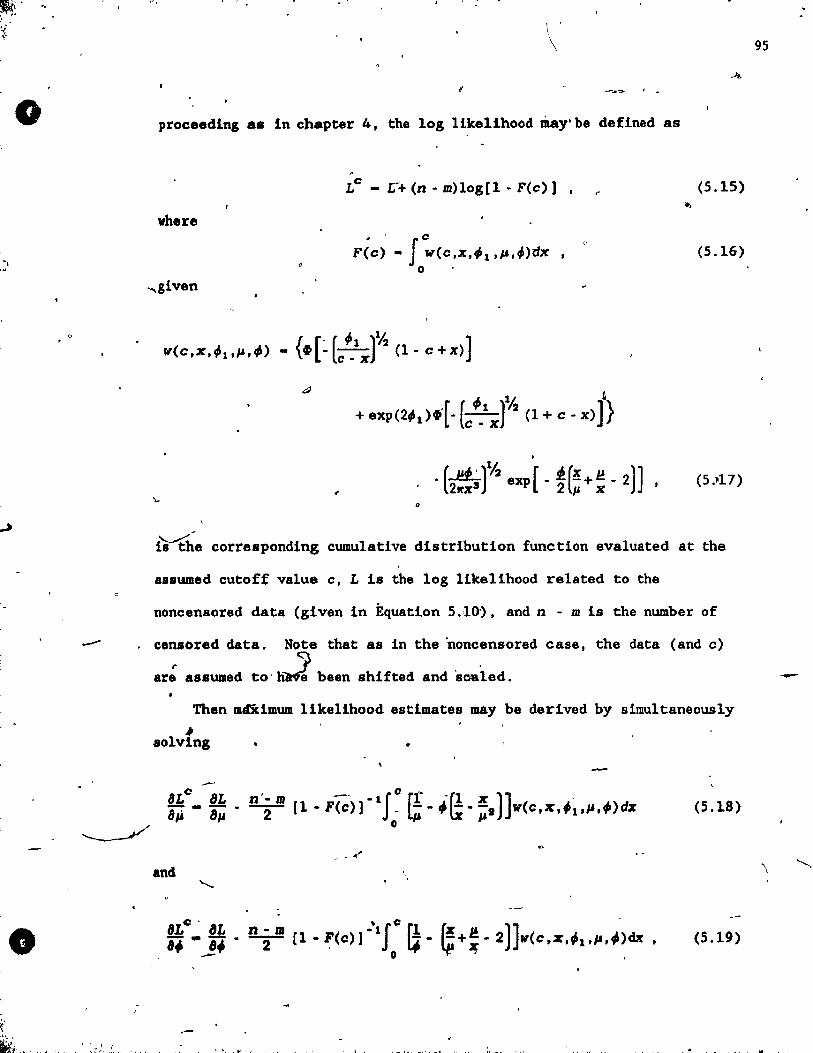
l!ii' . ~: . " L>~ -"i~
o
'"\ ...
• :~-\ , ~v 11ft .... , .
l';
\ . \
\
, .
proceeding .s in ehapter 4, the log like1ihood may'be defined as
where
"
~
Le _ r:+ (n - m)1og[l - F(c) ] ,
, c
Fic) - f W(C'%'~l,~,~)dx o .
(5.15)
(5.16 )
.....given
-
~
-,
.[ ( ~1 )% ]~} + exp(2~1)~ - c:x (1 + c - x)
,
. (...eL)% exp [ _ f.(!+M -2)] 2111'x' 2 JJ x '
(5 .• 17)
"
ij~he corresponding cumulative distribution function evaluated at the
assumed cutoff value c, L is the log like1ihood related to the
noncensored data (given in Équation 5.,10') 1 and n - m is the number of
censored data. Note that as in the noncensored case, the data (and c)
ar: 8s8umed tO'h~ been shifted and soaled.
Then mgximum 1ikelihood estimates may be derived by simu1taneous1y ~
Bo1ving
8LC aL n' .. m -' 1 JO [f . ~ x)] -. -- -r- [1 .. F(e)]- _ --.---1 w(e,1C,~~,II,~)dx (5.18) 8/À a", o Il '"
> .K
and \
"-
8Lc ' 8L n-JI [1 - F(c») -', ( ~ - ~+ ~ - 2 ))w(c ,z ,;,,l',~)dx (5.19) ~-iJ· -r --
-
95
-
\ ..........
-"
o
'.
..'
o
, '
I~
",
where the partial dérivatives of the noncensored log likelihood are ,
found in Equations 5.12 and 5.13. As vas the case in the prevlou8
• section, this approach Is Yery cdmputationa11y intensive.
Hodel1ng Components of Rc!sct:lon Times
One application for t~ convolution of two inverse Gaussien
distributions is the mo~ling of motor and decislon response ,
• oomponents. That i~, the random variables Tl and T~, defined in the
previous sections, wou1d be re1ated to motor and decision time .!
distributions, respectively.
In such a mode1ing application, the first step must invo1ve
,obtaining ';'otor Ume respon.e~ in ba.eline ~as w •• d~n. in
Burbeck's (1979) experiment by using a loud noise stimulus. Note that
.~ome minimal decision time is necessarily incorporated into these ,.
latencies. These baseline times are then fitted with a shiftad inverse
Gaussian distribution. Sorne theorètical justification for using the
inverse Gaussian to modal this eomponent might be found in physical ~ /
studies, such as those involving neural spike trains (e.g., Fienberg,
1974; Rodieck, Gerstein, & Kiang,' 1962).
This motor time distribution can then be convoluted wlth an~ther
inverse Gaussian re1ated to the decision time. Iess the minimum
deeision time absorbed by the first random variable. AI mentioned in
chapter 3, Burbeek and Luce (1982) showed "through a hazard function '
argument that among the we11-known 8ke~ed distribution. on1y the
-
96
-
.. c~
o
o
. ---- ", .. "",T.;'"
inverse Gaussian and Grice's random criterion mode1 (1968, ~972)
adequ~tely account for the commonly observed peaked hazar'i func tio~
associated with such 1atencies.
Figure 5.1 contains a convo1uted inverse ..Gaussian Q-Q plot of
- subject S. B. ' s data from the 250 Hz, 20 db condition of Burbeck' s
experiment. This plot is comparable to the shifted inve~e Gaussian Q-
Q plot found in Figure 4.1. The slight differences are evident in the
residual Q-Q plot given in Figure 5.2.
Table 5.1 contains moment estimates of convo1uted inverse Gaussian ~.
paràmeters for Burbeck's da~ As previ'Ous1y mentioned, the trials
employing loud noise stimuli were used ta estimate the parametei's QI'
/JI and ft. Go~dness-of-fit resu1ts are comparable to those obtained by
simply modeling the data with the shifted inverse Gaussian '" ,
diStribution.
A second application of these procedures ls to the classical
Donders' subtraction. paradigm. In this case the random variables Tl
and T2 correspond to the response times for two tasks which differ in
complexity. Such a situation existed in Link' s two-choice exper.iment
where responding' to Stimuli land 6.. was easier tha~_ ~or St1~uli 2, 3, 4
and 5'. . Table 5.2 contains the results of modeling the more complex
conditions as convolutions of inverse Gaussian distributions.
-- f
. ,~
...
97
1
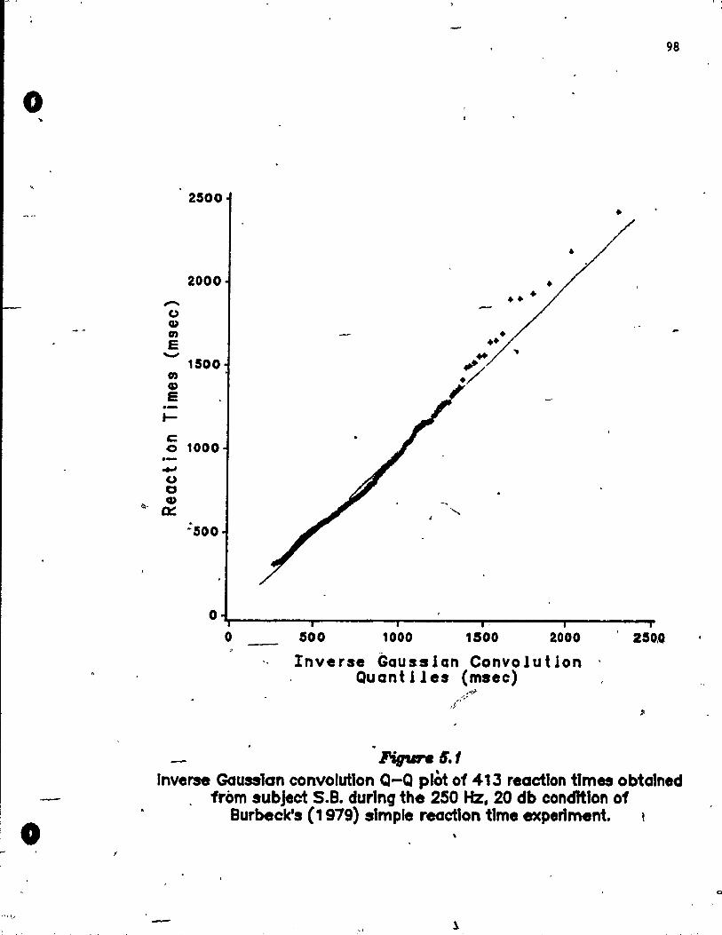
o ..
~
~-
o
,...... Co)
CD 0)
E ......, 0)
CD E .-~
c 0 .-...., (J
C CD
0:::
2500 •
• 2000
1500
1000
~500
O~--____ ~ ______ -r ______ ~~ ____ ~ ______ ~
o 500 1000 1500 2000
Inverse Gausslan Convolution ' Quantl1es (msec)
1'igvre 6.t
, 250,0
98
Inverse Gausslan convolutIon Q-Q plot of 413 reactlon tlmes obtalned from subJect S.8. durlng the 250 Hz, 20 db cond1tlon of
Burbeckls (, 979) sImple reactlon tlme experlment.
-
"\ .. ,
<:>
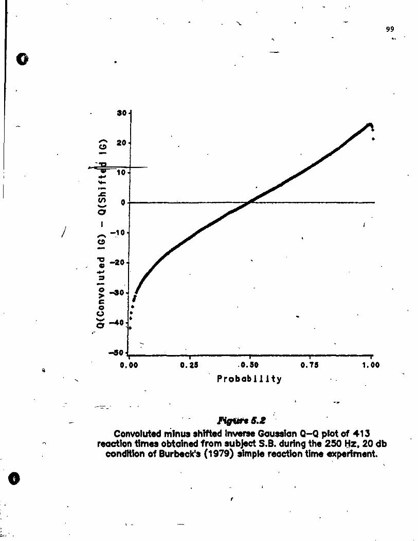
o
t
1
,"
e
., ~~I' ,
•
30
".... (!)
otJ 10
't-.-.J:. fn 0 ...... 0
1 -10
".... " (!)
-g -20 CU
otJ ~ -
-ao.-________ ~--------~--------~------~ 0.00 0.25 .0.50
Probabll1ty
".,.....'.R
0.15 1.00 ..
99
Convoluted minus sh1fted Inverse Gau_tan Q-Q plot of 413 reactton tlmea obtalned from subject S.8. durlng the 250 I:fz. 20 db
cond1tlon of Burbeck's (1979) stmple reactlon tlme expertment.
r
\ -
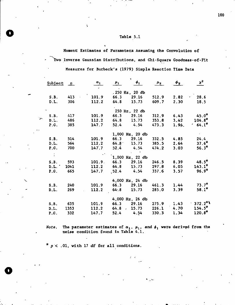
o
')'.
. . o
.. -.,.... ,<r ..... ~.,. .
Table 5.1
Moment Estimates of Paramete~ Assuming the Convolution of
~o Inverse Gaussian Distributions, and Chi-Square Goodness-of-Fit , "
Measures for Burbeck's (1979) Simple Reaction Time Data
Subject n
S.B. D.L.
S.B. D.L. P.G.
S.B. D.L. P.G.
S.B. D.L .. P.G.
S .B.. D.L.
S.B. D.L. P.G.
413 306
417 486 385
514 564 700
593 1041 665
240 269
635 1353
332
101.9 112.2
101.9 112.2 147.7
101.9 112.2 141'.7
101.9, 112.2 147.7
101.9 112.2
101.9 112.2 147.7
~l
. 250 Hz, 20 db 66.3 29.16 512.9 64.8 15.73 609.7
250 Hz, 22 db 66.3 29.16 64.8 15.73 52.4 4.54
1,000 Hz, 20 db 66.3 29.16 64.S' 15.73 52.4 4.54
1,000 Hz, 22 db 66.3 29.16 64.8 15.73 52.4 4.54
4,000 Hz, 24 db
312.9 353.8 473.3
332.5 385.5 474.2
246.5 29T.8 337.6
66.3 29.16 461.3 64~8 15.73 285.0
4,00-0 Hz, 26 db 66.3 29.16 64.8 ~ 15.73 52.4 4.~4
275.9 226.1 330.3
2.82 " 28.6 2.30 18.5
6.43 3.42 1. 9~_
4.85 2.64 3.03
8.39 6.05 3.57
1.44 3.l9
1.43 4.70 1.34
45.0* 104.8*
. 64.1*
24.4 37.6* 56.3*
48.5* 143.1*
96.9*
73.7* 58.1*
372.2*\ 154.5* 120.8*
Note. The parameter estimates of °1 , ~l' and ~1 were deriv,d from the noise condition found in Table 4.1.
* p'< .01, with 17 dE for al1.conditlons.
: <
100
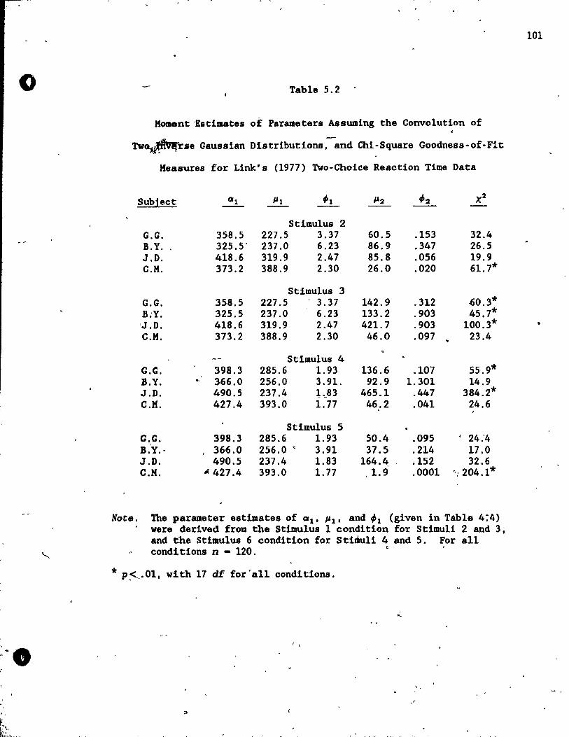
0 Table 5.2
Moment ~stimates of Parameters Assuming the Convolution of •
Tw~~rse Gaussian Distributions,--and Chi-Square Goodness-of-Fit .
Keasures for Link's (1977) Two-Choice Reaction Time Data
Sublect Ql 1-'1 fi P2 f2 X2
Stimulus 2 G.G. 358.5 227.5 3.37 60.5 .153 32.4 B.Y. 325.5' 237.0 6.23 86.9 .347 26.5 J.O. 418.6 319.9 2.47 85.8 .056 19.9 C.K. 373.2 388.9 2.30 26.0 .020 61.7*
Stimulus 3 G.G. 358.5 227.5 3.37 142.9 .312 -60.3* B:Y. 325.5 237.0 6.23 133.2 .903 45.7* 'J.D. 418.6 319.9 2.47 421.7 .903 100.3* C.K. 373.2 388.9 2.30 46.0 .097 .. 23.4
Stimulus 4 G.G. 398.3 285.6 1.93 136.6 .107 55.9* B.Y. 366.0 256.0 3.91. 92.9 1.301 14.9 J.D. 490.5 237.4 t._83 465.1 .447 384.2* C.M. 427.4 393.0 1.77 46.2 .041 24.6 ,
Stimulus 5 G,G, 398.3 285.6 1.93 50.4 .095 • 24.'4 B:Y.- 366.0 256.0 c 3.91 37.5 .214 17.0 J.O. 490.5 237.4 1.83 164.4; .152 32.6 C.M. - 427.4 393.0 1.77 ,1.9 .0001 ": 204.1*
Note. The parameter estimate, of QI' 1-'1' and ~1 (given in Table 4:4) were derived from the Stimulus 1 condition for Stimuli 2 and 3, and the Stimulus 6 condition for Stimuli 4 and 5. For a11 condi tions n _ 120. 0'
* p,.Ol, with 17 dE for"a1l conditions.
, ,
'.
101
.. -
o
o
. "
Chapter 6
Confidence Intervals and Statistical Inference
Larg~ Sample Test:s
~nlike the nonshifted inverse Gaussian case-exact tests are not
ava!lable for the maximum. likelihood estimates developed in chapters 4
and 5. However, one.may use generai large sample procedures to create
'confidence intervals or envelopes and provide statistical Inference. ,
For a more'complete description of the procedures discussed in this
section~ Rao (1973, chap. 6) may be consulted.
Three main types of large sample tests are currently avaHable.
These are based on the likelihood rat:l0 (Neyman & Pearson, 1928), Wald
(Wald, 1943), ànd Lagrange mult:lplier (Rao. 1948) ~atistics which are
deno~ed in this thesis by LR. W, and-tM, respectively. As observations
are restricted by the shift parameter, the three-parameter inverse.
Gaussian vio1ates the usual regularlty conditions. Desplte this, the
maximum lik~1ihood estimates for t~e shifted inverse Gaussian pOlsess
the necessary normality and efficfency properties which these three
tests require (Cheng & Amin, 1981).
For simple hypotheses of the k!n.d Ho: , - '0 versus Hl: , .. '0" where , and '0 are parame ter vectors, tbe likelihood ratio crit.rion i.
/
(6.1)
102
o
1-
• ~. '
~;.:~ ':.'
'\
1
1
--103
,. where L(') and L('o) are the log likellhoods glven. the maxl~.
,. l1kellhood eatlmate , and flxed 'o, respect~lely.
'\ The Wald statlstlc is given by
A - , A A '
W - (1 - '0) I(')(' - '0> 0(6.2),
where the expeéted informatio~ matrix I(') is defined as
As 'the observed information matrix •
-'
CC')
is'~ consistent estlmator of I('~, It is often ~s~d in place of the . .
expeç~d information matrix given in E~uatlon 6.2.
The ~grange multiplier statistlc is . -
w)\ere- SC') la the vector 'af first derivatives of L(I). Note that in "
thi. case'the expllclt maximum likelihood estimates are not needed. . . , Also. as wlth the Wald statistic, the expected information matrix m~y
\
be replaced by the co~responding observed information matrix . .
The asympt.Qt1c distribution of a11 three statistt~s is chi-square _
..
'.
. , n'
o
,
. , o
with k ~egrees of freed.om. "That i,s,
LR ! W ! LK - X2 (k) (6.6)
where k ia the length 0t. the vectors,' and ,'o' Using çhis fac~.
confidence intervals (or enve1opes) and tests of significance may be , ' developed f~r a wide variety of applications.
C~mposite hypotheses of the t~e Ho: r(I) '- 0 versus Hl:~r(') ~ 0,
for,a specifiêd function r(')l may a1so, ~e,han~led in a similar way.
ln this case the like1ihood ratio criterion la glven by
1
--1\ !..
LR - 2 [L(') - L(')] t(
1 ,
(6.1>
where i i's the maximum likelihood estlmate of '" restricted by' the nu11 , ~.
hypothesis flo: r(I) - O.
_" The corr.effpondlng Wald statistic i8
-(6.8)
t f 1\ whe're R. is a matrix of partial detivatlyes of r(I) evalua ed et '. and
asauming that the inv~rse exists.
Finally, the Lagrange multiplier criterion Is glven by
104
... . . ~ .. , ,.'
, (6.9)
, . , where agaln ï is the lIaxilR\1lll likel1hood estlmate of ',- .restrieted by
. '
\
! '
.'
J '
o
, '
- 105 , i ,
'1 f . th~ nuÙ hypothesis Ho: r(I) - O.
i ~e. asymptotic di~~ribution ôf these thr~e latter forms of the j.
'st!at1stics 1s also chi-square with ~egrees of freedom dependent- on the !
n~ber of restrictions placed on, , by the null hypothes~s." Whl1e the .
rJlative merits of the~e thre~~~ests have bAen explored by a number of
iri.lestigators (e'.g., Berndt & Savin, 1977; Buse, 1982; Chandra & Joshi, 1
19r3; Fisher & McA1eer, 1980), more research is needed before a final
cobsensus' can be reached. ,1
• J ", Shlftfd Inve~se Gausslan Procedures
..
l, l, ,~e shifted inverse Gaussian maximum 1ikelihood parameter
eifimates and 1o~ likelihood function needed to perfo~ 1ikellhood 1 -
ratio ,tests are given in chapter 4. As mentioned in the p,revious 1
'section, the' c6rresponding o~served or expect~d information matrix is ,---, require,d to fOrDJ the Wal.(i and Lagl!ange multiplier statistics. the -
." \. ' "
~ : "followf~g are the components of ~he observeçl information matr1x:
1
1 l'
J.
. "
, "
• t
...
.,
.. , "
, .
1 -,
. \ .
", r ••
0,
-t
v
0
- .
" .. ' and. -. -
-(6.10)
The expected information matrix èân'be ~btainéd by lnyerting the . ' -
asymptotic covariance matrix (uij), wher~ u~J ~n~l&ijk·l with ....
,- -
. . ~22 - p· ... ;-l <t + ~;-2 +- 3;-3)
- .. .. .
. (6.11)
and
k . . (6.12) ..
These results we~e derlved from formu1ae given by Cheng ~nd Amin
(1981). Note that the subscrlpts
a,l-'. and ;,' rè~pectivély. r-' 1. 2.. aqd 3 'ln Equation 6. il ,refè; . to . - - . -
> ' ) ,q
. Givèn in table 6:1 are-the results o~ a' Montè Carlo .tudYon the
1
J .... l' , _
1\" , .-.....
'.
. 106
..
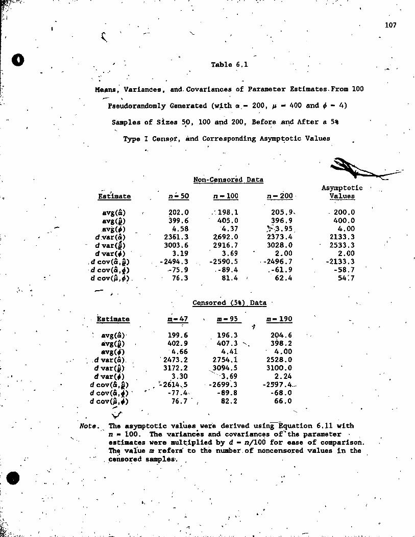
... :t '~t("'!f~-,",
: /
~i
o
-
, . . , ,
~'. '.
) ),'L
~';'\
" ,
.. .,!- ~ 4,._) ,_./f.,;-
Table 6.1 . "
Me_os,' Variances, and, Covariances of Parameter Estimates.From 100 -Pseudorandom1y Generated (w~th a,- 200, # - 400 and ~ - 4)
Sàœp1es of Slzes ~O. 100 apd 200, Befo~e a~d After a 5% "
Type l Censpt, and Corresponding Asymp~otic Values d,
Non-Censoréd Data
Estlmate n':' 50 n-100 n- 200, ASymptotic
Values
avg(~) 202.0 avg(~) 399.6 _avg(;) 4.58
d,var(&) 2361.3 dvar(~) 3003.6 dvar(;) 3.19
,d cov(&,i> -2494.3 'd cov(&,~) ,-75.9 d cov(p,~>_ 76.3
- f
Estilll!te !J3- 47 r
avg(~)' 199.6 avg(i> 402.9 avg(;) '4.66
,dvar(&), '2473.2 dvar(i) 3172.2 dvar(;) 3,30
d cov(&,i> • r:. 26;1.4 •. 5 d cov(&,~)' -17 .4· d cov(p,.) 76.7 . ....
V
.',198.1 205.9, 405.0 396.9 '4.37 ~,,3. 95,
Z692.0 2373.4 2916.7 3028.0
3.69 2.00 -2590.5 ,-2496.7
' -89.4 . -61. 9 81.4 , 62.4
Ce,nsored (.5'>' Data
m-95 m-190 ., 196.3 204.6 407.3 ..... . 398.2
4.41 4.00 2754.i 2528.0 ~094.5 3100.0
'-3.69 2.24 ' -2699:3 -2597.4 __
-89.8 -68.0 82.2 66.0
"-
·200.0 400.0
4.00 2133.3 2533.3
2.00 -2133.3
-58.7 54:7
, ,
Note. The asymptotic values were derived using Equation 6.;1.1 with " n .. 100. The v:ar1ances and covarlanc~s of'the parame ter . ,
eseimates were mult,lplied by d - n/lOO for ease of comparlson. The varue m refera to the nUDher,of noncensored values in the
, .c:e~so~ed $8D!PléS" .
.'
•• . , .' "l'
107
,,,,
. ,
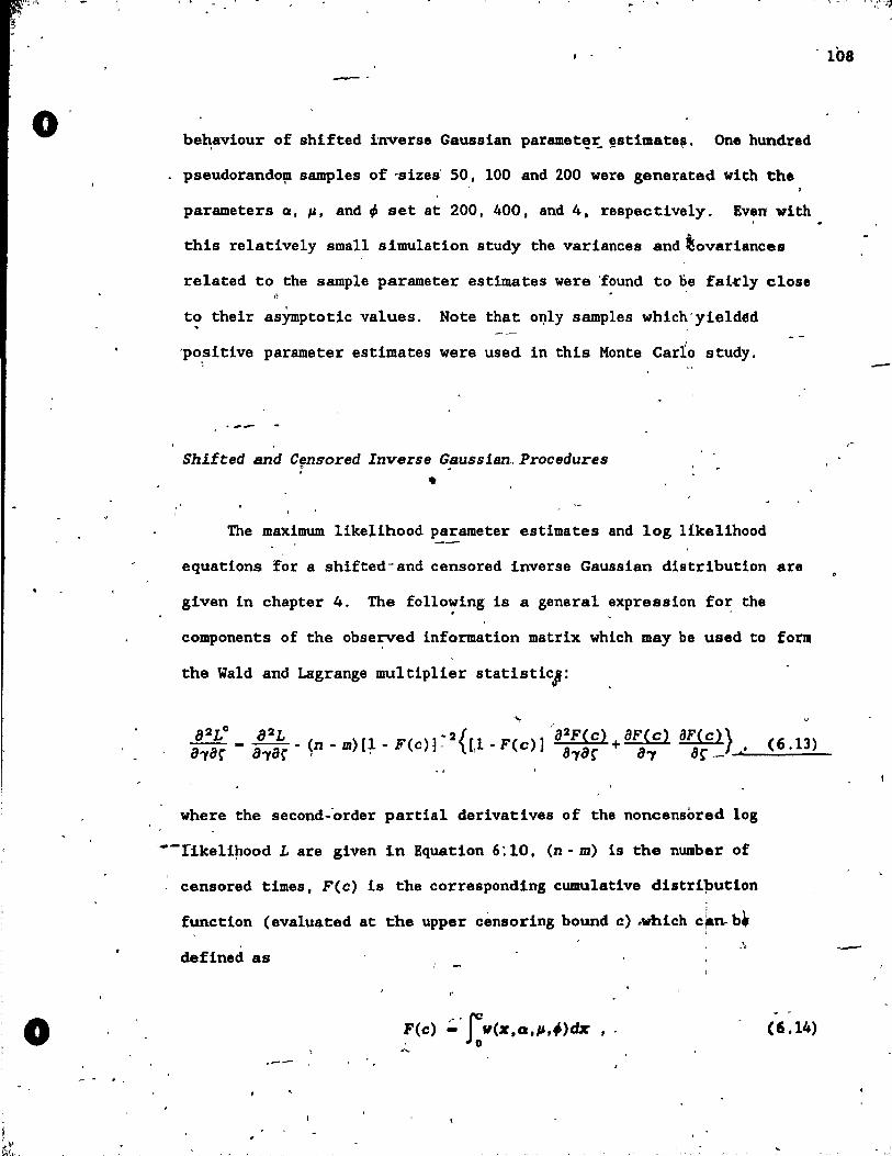
o - '.
, . - 108
behaviour of shifted inverse Gaussian paramet!x:. !stimate,. One hundred
pseudorando~ samp1es of 'sizes' 50, 100 and 200 were generated with the
parameters Q.I-'. and'" set at 200. 400, and 4, respectively. Even' with
this relatively smal,l simulation study the variances and ~ovariance8
related to the sample parame ter estimates were 'found to De fai~ly close
t? their aSYmptotic values. Note that o~ly samples which'yielded
'po~sitive parameter estimates were used in this Monte Carlo study.
Shlfted and C~nsored Inverse Gausslan .. Procedures
• The maximum likelihood parameter estimates and log like1ihood
equations for a shifted-and censored inverse Gaussian distribution are
given in chapter 4. The follo~ing is a general expression for the
components of the ~bse~ed information matrix which May be used to form
the Wald and Lagrange multiplier statistic#:
...,
a2 Lo
_ 8 2 L _ (n _ m) [1 _ F(c) 1 ~2{[1 _ F(c)] / 82F(c) + 8F(c) 8F(c)} (6.13) a..,ar a..,ar l ' 1 1 a..,ar a., ar _ ............ --:;.-----
where the second-'order partial derivatives of the noncensored log
· ... -rikeli~ood Lare given in Equation 6: 10, (n - m) 1s the number of
censored times, F(c) 1s the corresponding cumulative distripution i
function (evaluated at the upper censoring bound c) .which crn- b •
•• defined as
.--(6.14)
--
-
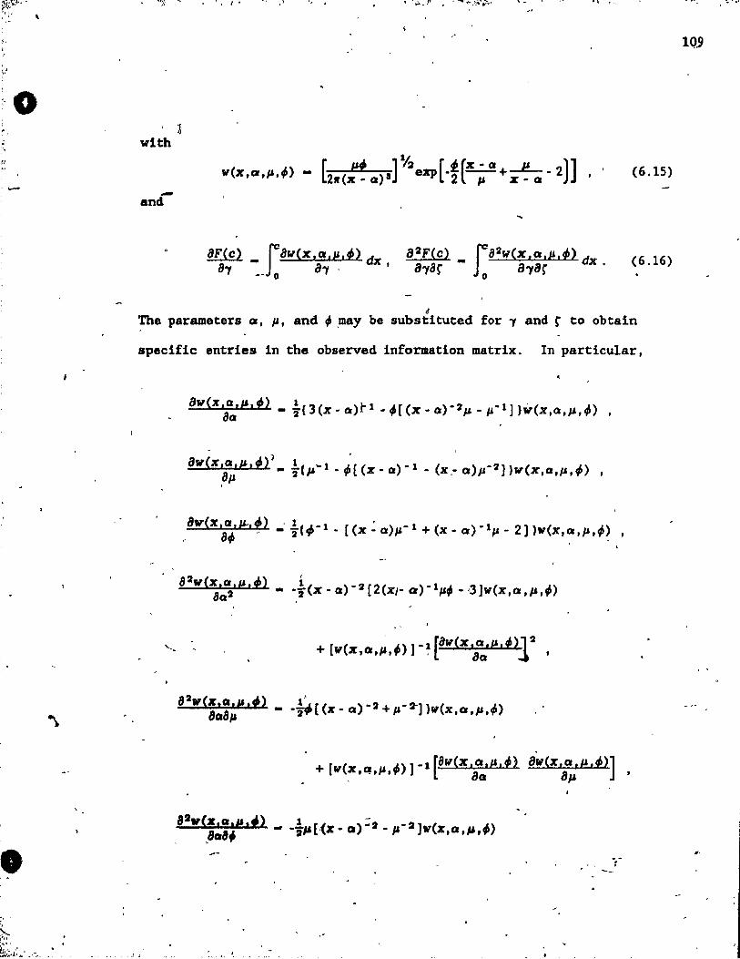
~1~;~" " 'l ~, , '
,<,
,.'
•
, l with
-and
i"." ... ,. .f ~ "'... •
.'
8F(c) _ [8W(x.a,J.!,f) dx 8"1 __ 0 8"1 ' '
"\""- ...,
(6.15)
(6.16)
<$
The parameters a, p, and; ,may be substltuted for "1 and r to obtain
specifie entries in the observed information matrix. In particular,
.. ) f 1
8w(x,a,M,;) l( "'1 "[( )-1 ( ) -2}} ( ") ,8p - '2 JI -.,. x-a - K,-a p W x,a,p,'I' ,
8w(x,a,I'-,;) '1(..1.-1 [( , ) -1 ( )-1 2]) ( ") 8; " - '2 '1' - X - a p + x - cr p - W K, ~ • P • .,. .
. J J "
-:""'.-'
lQ9
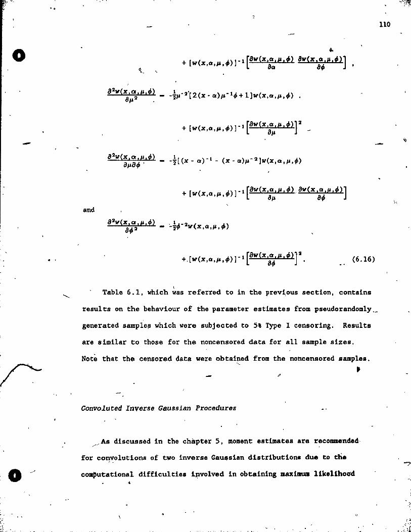
o
-
, , 1
o
)-, . ~~ ...
.. ~ ,~ .,.
and
a2w(x,Q,p,f) al'a~ .
0-
+ [W(X,O,p,~)]·l [aW(X'a':'P';) 8W(X'a~'''';)] ,
+ [ ( "')]-1 [8w(x,o,p,;>,aw(x,o,I";)] w X,O,P,." al-' a~
(6.16)
l
Table 6.1, which was referred to in the prev~ous section, contains
results on the behaviour of the parame ter estimates from pseudorandom1y __
generated sample~ which were subjected to 5% Type 1 censoring. Results
are simi1ar to those for the noncensored data for a11 samp1e sizes.
Notè that the censored data were obtained from the noncensored samp1es. '- • . '
Convoluted Inverse Gausslan Procedures
r-' As discussed in the chàpter 5, moment estimates are recommended
for convolutions of two inverse Gau.sian distribution. due to the , -
computational difficu1ties i~vo1ved in obtaining maximum l1kel1hoad ~
110
:i ' . . ~ ~ f.).
.. .'.; ~I~

. __ .. _._-~
,/ o
, \
o
1
"
•
estimates. However, it is still possible to perform certain large
sample -tests which usually require maximum l1kelihood es t iJlla tes , with
relatively little computational ~fort.
Conslder the likelihood ratio approach. .!wo basic statistics are
needed in this case. First, the restricted log likel1hood 15 required.
which can be easily obtained in cases where the parameters are fixed to
specifIe values. Second, the overall maximum likelihood esti.mate ls
needed. Whlle the exact maximum m,sy be difficult to achieve, a tight
bound around 1t 15 easlly found using the' interval search technique
discussed in chapter 5. The resu1 ts from this bound May be sufficient
for many testing. situations.
-•
(
, .
, .
111
o
"
. o
Chapter 7
Discussion
Inverse Gaussian Versus Lognormal DIst:r ibutions
The goal of this thesis has been to explore new approaches tQ
analysing skewed latency data. By reason of its skewed shape, random f
walk rationale and convenient s tatistical properties, the inverse
.' Gaussian distribution was used as a basis for this investigation. This
is in contrast to the usual lognormal approach upon which many
psychologists rely today, and it is therefore natural to assess the
usefulness of the inverse Gaussian by comparing its performance with
that of the' lognormal distribution.
As discussed in chapter 3 the inverse Gaussian has been employed
to provide a random walk model for certain reaction time distributions.
Modifications to the definition of this distribution, as in Link and
Heath' s (1975) relative judgment theory, have sinee been shown to model ,
data better than the original form. Still, the earlier results
indicate the similarity of the process fres which the inverse Gaussian
arises and the types of theoretical processes whieh some psychologist~
believe explain many kinds of latency distrib~tions.
The lognorma'l, distribution, on the other nand, is usually used to
analyse latency data simply due to its skewed nature .. A inUl\Pl1Cative
underlying process would "'ftecessarily have to be assumed beforel the
1
112
(;
-"
o ',"
, .
lognormal could' be seriously considered as a model for any response
time data. So from a theoretical viewpoint, as additive processes are
more commonly assumed, the inverse Gaussian currently fares better than
the lognonnai as a basis for analysing 1atency data.
Whether orJlot lt is imp.ortant that a distribution conforms
theoretica11y with the process underlying observed data will depend in
" part on the goals of specifie experiments. For examp1e, if on1y group
differences are of interest then the choice of distribution might be
" made on the basis of general fit and ease of statistical inference
alone. Even in this case, however, when a dis tribution has a
o
reasonable ftheoreti"cal basis an investigator shouid have more
confidence inoits abllity to fit unfami1iar data.
From a" statistical viewpoint, the two distributions can be
compared in° terms of their sufficlent statistics. The sample
arithmetic and harmonie means are suffici'ent statistlcs for the inverse
Gaussian. The arithmetic mean (as dlscussed in chapter 1) ls an
,~ appropriate average to use when an additive process is postulated and a
. ~ . . fixed response ls stil'ulated. The harmonie me an , which 19 ealcu1ated
from the reciprocals of observed values. can be used to obtain
inferences concerning the average speed of response.
In comparison, the suffident statistics for the lognormal
distribution are functions of the geomecric mean and the sum of squares
of the logged data. These statistics are interesting ~nly rhen a
IllUltlpl1c~tive process is postulated. \'
The overall fits of the basic inverse Gaussian and lognorma1
distributions to Burbeck (1979) and Link' s (1977) data werè found to' be
t
/
1
113
114
o quite similar. Results from chapter 4 indicate that the adâition Qf a
shift parameter substantially improves the abUity of the two
distributions to model latency data. However,. goodness-of-fit
differences between the two three-pat'ameter distributions were also
found to be very ~~al1.
In terms of computing maximum likelihood parame ter estimates the
basic distributions were found to be comparable. However, when a shift
parame ter is added important differences become evident. The three-
parame ter lognormal likelihood function attains a global maximum when
the' estimate of the shift parameter equals the minimum observed value,
whieh is not a sensible result. Hence, an investigator must be
satisfied with only a local maximum in the case of the lognormal. ln a
study by Cohen and Whitten (1980). 14 .. dU/ferent shifted lognormal
estimates were compared. The authors recommended the use of different
estimates depending on the data at hand. By employi~g the inverse
Gaussian distribution, these complic_ations can be avoided sinee the
corresponding maximum likelihood estimate of the shift parameter 18
always less than the minimum sample value when the data are positively
skewed.
In terms of statistical inference. the two basic dis tr1butions are
virtually equivalent with respect to the testtng of simple hypotheself. , -..
Vith respect to complex experimental designs, the lognormal- was found
to be much more versàtile. However, future rel!~arch will certainly be
done to explore the applicablity of the inverse Gau~sian to such
designs. In any case, how well a distribution allows for tests of
o. significance is uPimportarf the sample statistlcs lt uses .re not of
..
o
•
. "'7'" ,- "j'.- ~ J
c
interest. For example, many psyehologists ~ight not ehoose the
geometric meAn to 4escribe their latency data, but have been fOTced to
do so in the past due to a lack of alternatives. to the lognorma~
,taeistical model._
While exact tests are currently unavafla~le for both the inverse
G~ssian and lognormal three-parameter distributions, the large sample , ,
tests described -!n- chapter 6, may be 'applied by using either. 'ln the " .
lognormal case as the only reasonable maxima are local an added degree
" of uncertainty is incorporated into any of the general maximUin ,-
likelihood test procedures. For example, particular ~ypotheses may not , .
be rejected using a shifted lognormal simply because the globar maximum . '.>' . ,
was not achieved. By uslng the three-parameter inverse Gaussian ) " . . )
distribution this prohlem may be, avoided. {
Hodifylng the Inverse GlIusslsn Distribution
. ,As indicated in chapter 4, the addition of a shift parame ter
greatly lmproves the mod~ling capabilities of the inverse Gaussian , .~
distribution. Including a t~ird parameter~ may also provide . ,
invest~gators with some.interesting ~emental inf~!Mati~n. Consider .. - \ \ . '
the results from the noise condition in Burbeck' s simple re~ction time'
experiment found in Tables 3.i and 4.1. Subjects D.L. and S.B.
obtained Mean reaction'times'of 177 asec and 168.3 asec, respectively,
in~ica~ing that D. L. was slightly faster. However. the t;hree
paraaetar Invér.sè Gauss1a~ estiaates of P" in order. were 64.8 msec and
\
. ,
115
o
)
, .
•
66.3'msec. suggesting th~t a different interpretation of events.may
emerge a~te,r shift parametfrs are partiaHed out. This pnenomenon vas
81so 'found in a number of other conditions. Clearly, if psycqologlsts, •
look beyond simple 1Deans, novel and illtriguing results Mar be found .
. Of course, the theoretical Interpretation of the shift parameter
depends on the expe~imental situation at hand. l ,
ln a similar manner, the ~onvolution of two-inver~e Gaussien ,
distributions can provide investigators with additional insight. ln
Burbeck's experiment the Mean response time differences between
subjects S.B. and P.G. may bè reduced by approximately 32 msec if their ->---
respective minimum motor times ate partialled out (as shown in ~able '
5.1). During Condition 2 in Link's two-choice reaction time ... experime'nt, subjects B. Y. and J .D. obtained mean response times 'of ,
649.4 msec and 824.2 msec, respectively. However, in terms of the
a"dded c'omplexity of Stimulus 2 over Stimulus l, these subj ects were
estimated to have 'average response tim~s of 86.9 msec and 85.8 msec,
• respectively <as shown in Table 5.2). .
The results from chapter 4 clearly indicate that added estimation
precision .is obtained when censoring iB properly.handled. In' addition,
the censori~g teèhniques developed in this thesis might be used to
in~estigate distributional changes in the upper tail. In certain cases
s~bjects may start to react differently ~f they have not responded
within a' certain' eime perlQd. Compar1ng results before and ~fter.
censoring portions of the upper taU might' provide evldence of 8~eh a.
phenomenoD;. •
116
'"
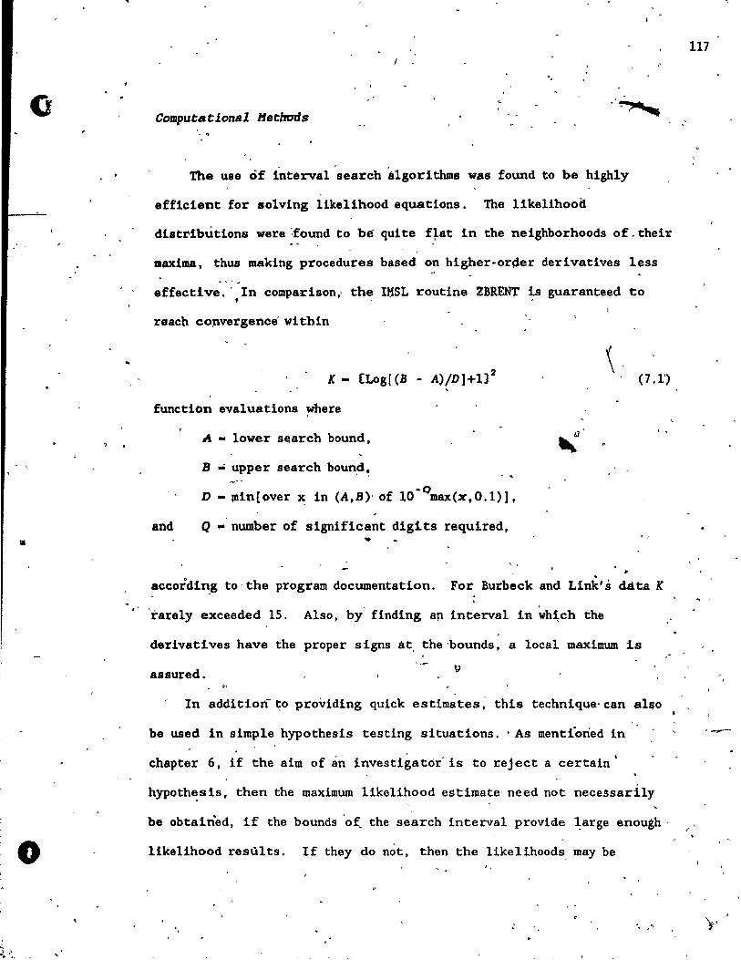
•
o
.. "
f
'.
Computatlonsl Hethotls
The use of lntervai 'search èlgorithms was found to be highly
efficient for solving likelihood equations. The likelihood
distribùt10ns were ~found to be quite f~at in the neighborhoods of _ thei:r
maxima, thus making procedures based on higher-orger derivatives less
effective. ' In comparison,' the l~SL routine Z8R.ENT is guaranteed to ,
reaab co~vergence within
K - {Log( (B - - A)/D]+U2
(7.1')
function evaluations wbere
A - Iower search bound, , .
B .. upper search boun~~
-Q D - œin[over X: in (A,B)' of 10 max(x,O.1)],
and Q .' number of significant digits required, .. , ,
accordin.g to' the program documentation. For Burbeck and Link' s dàta K
" 'tarely exceeded 15. Also, by' finding ap intervai in ~h~ch the
derivatives have the proper signs At, the 'bounds, a local maximum is
assured. "
In addition to providing quick estimates: this technique- can abo
be used in simple hypothesis testing situations .. As mentloried in
• , ' - 1
chapter 6, if the aim of an investigator is to t;eject a certain
hypoth~sis, then the maximum likelihood estima~e néed not neceasarily
be obtained, if the bounds 'ot:. the search interval provide ~arge enough -
likelihood resùlts. If they do not, then the likelihoods may be "
" -,
117
..
. -.--
o
o
....
, checked conti~uously as tbe interval 'is shortenéd. Clearly th!s ia a
convenient procedure for many computationally intense problellls. . . Unfortunately, an interval seareh algor.ithm can only be appUed to . -
solving single l1kelihood equations. ' With addi"t:ional research. a grld , . ""
type search procedure may be developed for solving the simul,taneous ;
Uk~lihood equations given in this thesis.
Conclusions
Latency data have been used extensive1.y in psychologiea), rese~~ch, -
and will' certainl:y continue to be used in the future. Currently.
lognormal statistical methods are commonly utlliz.ed to analyse thè~e
data. 'These procedures do not ~ake into consideration màny of the ,
~~aracteristics which ~re 'P~rticular to latency data.. Thus'
invéstigâtors ~ould profit from some general analysis te'chniques which
do. t· '. " .. Tl)is thes 1s indicates that the inver~ Gaussian provides-a
, , " reasQ..nable alternative to thèjognormal distribution as a basis for a
, v.ariety of statistical'analyJs: This distrib,!~ion confo~s ~IO.ely to
frandom walk models of reaction times and is characterized .by sensible'
" statistics, such as the ari thmetJ.c and harmonie me~ns. The associated
exact sampling theory allows for tests of signipi~anee, similar to
---Student' s t test and Qne-way ANOVA, to ~e performed on nontt:ansformed
data.
Adding a shife parame ter to the definition of the inverse Gaussian f#
"
118
.; ~I'-_ ..
. ' ,
..
"
o ,.'.
•
'. , . , .
wa. fo~d to improve 'the fit of the .nodel ~o reacdon tlme data.
C~nsori~g w.as- als,handleci easily 'in' thl.s -case:. Dedding whether. thi,s
addition of a ahi~ t parame ter is necessary depends in l'art on th~
'l'obus.htesB of the tatistical procedure being considereC1. On thè otller.: \ ( , ,
hand. the shift pll:r~~ter does provlde additional' inf~rmation: about the <>
nature of the underlying process, and May be subtracted OUO to allow , . experimenters to ooncentrate o~ i~dividual decision,times,
Similarly, convolutions pro~de added insight with regards ta the' • • "' 1
unde'rlying processes ~hich. produce observed values', Th~y also provide
investigators wlt~ the chanc~ to p~rtiàt out individual minimum:r ,
reaction,times which can affect subsequent analyses. Also as a result,
the Donders subtraction method May be applied not only to œean tiJnes 1ft' • '
but as well 'to the distributions associated with the s~bcomponents.
When this thesis was initiated the int:e'nded goal was to introduce
the irtvetse Gàusslan as' a basis for statistical analyses of ,1a'tén~y -~ ,
data and to illustrate how thls distribut~~h May be modified in order , -
to help answer certain experimental questions 'iI) a sensible, mo.del-~ ~~ "
based; and efficient man~er. This necesaitated the cover~ge of a wide
rang~' of topics and applications. As with ma!ly other studies which -.,
involve an overvlew of a subject, some of the finer de"tails have been· .~ \
ollltted or left unfinished. ,
Another general problem ,invol ved the use of a personal comp~ter
for ~~l statistical analyses. The original intention was to ensure
that the presented procedures would not be so computationally intensive
that potential users .would fea.r the resulting costs. Unfortunately,
this restriction resulted, in the need for approximations in some ar~as.
-
119
...... "./
o
:
o
, 0 <J '. 1
120'" < ''J
• 0 . ,
~ î
1.... 1 . . / .
.For,. example, ex~ct 1Daxim~ ,w..kelihood e~t~ma~es of paraméters asauming//. " ,.,,' ,I~'
a ~onvolution model (given in ehapter 5) were not ealeulated.fof the ' , , , \
1
two reaction time sample 'sets due tb .the limitations'of the p~,onal ~ r' '
co~puter used. 1
" , Other areas which eould- have b~en given- more attention include th."
probléms with homogeneity of;varianee assumptions in experim~ntal
des1gns., s'man sample 'resul,ts, assessing thè power assoeiated with the , . vafious pr~posed testa,. and the use of average apeed' as the pr,incipal
, measure of central teridency.
1 •
Despite it1bd~fic:ten~ie's 1 ho'pefully this thesis has show the. , .
'grea,t p,0tential of the invers~ Gaussian with respect to analysing
psychologieal latency datà. In order for th,"s dis-t~i1?uti.on to gain , , i ,
br?ader acceptence, the, assoeiated statisticàl test$ will J'leed to be
applied to a much wider varl~ty'of response ti~e data 1 Substantial
'sim~lation' s~udies 'are also required ~o il1ustrate.thé more subtle , - ... ,1 \ " ... 1 ~
differenee~ bétWeen the inverse Gaussian and lognormal statistical . . \
, . ~ " (, '
models. In, addition; ehe devel~pment of .li ge~era~ inverse Gaussian .. - ,.... - . • ~ ..... r - . ..' " .. II ,.
s,tatistical computer p~.eléage would eertainly' improve acee~8abllfty to " ~ - \ \ .
thb.sensible alt'E!rnattye." ,".
"
, ..
'.
\ '.
, . ~
" '
•• ,1
" .
, , , .
>,
, . . ,-
" , ,
\'" ",
\
., .
o
"
. ,
~ - • ,~~ t - '.
..- . .
.,
References '-""
Banerjee, A. K~ (1986). A bivariate Inverse Gaussian dlstribue'lo';
'(R,eport No. "782). Madison, YI: University of Yisconsill, Department
of Statistics. ,
'Ban~rjee, A. K., & Bhat~acharyya, G. R.· (1976). A purchase incidence
, " model with inverse Gaussian interpurchase times. Journal of the " ". Amerlcan StatlstlC!al AssocJ.atlon', 7i, 823"829. 1
Banerjee, A. K. 1 & Bhat~acharyya. G. R .• ' '(1979). Bayesian" resu1ts' for
121
, ,.
.. .
•
the inverse ~aussian distr~bution with an application.
Technome~rlcs, 21, 247-251. , 1
-. Barndorff-,Nielsen, O. (1978). Hyperbo1ic distributions and
·aistributions on hypexbo1ae. Scandinavian Journal 'of Statlstlcs, S,
151-157.
Ba:t:tlett, 'M. S. (1966). 'An introductIon to stochastlc pracesses.
London:' Cambridge University Press.
'. Be.~dt, 'g. R~, ~ S~vin, :~r. E. (1977). Contlict among criteria for . .
testing hypotheses ,in multivariate linear regression modêl •
Econom~trlca, ~7, 203-208.
,Bickel, P. J •• ,& Doksum, K. A. (1981) . • •• "f;
~ ana1ysis of transformations
. revisited. Journal of the American Statlstlcal AssocIation, 76,
296- 311.-
BloxoaJ B. (1985). Considerations in psychometrie modeling of
. r •• porufe°tiae. Psychometrib. sa, 383-397 .
Box, ,G. E."". (1953). Non-n~rmality and tests on variance .
• r
"
0,
1
o
" " ,,"~", ".:" "" ." .,..:: .. ~~~ .:~
Biomet~lka, 40, 318-335. ~,
Box', G. E. P., (. Cox, D. R. (1964). An anA1ysis of transformations. - -'
Journal of the Royal Statistical SocIety, SerIes B, 26, 211-243, ,
Bradley, J. V. (1980a). Nonrobustness in c1assica1 tests on means and
variances: A 1arge-scale sampl~ng study. Bulletin of the ,
Psychonomic SocIety, 15, 275-278.
Bradley, J. V. (1980b)., Nonrobus~ness in one- sample Z and t test~: A'
large-sca1e samp1ing study. Bulletin of the Psychonomic SocIety,
15, 275-278.
Bradley, J. V. (1980c). Nonrobustness in Z, t, and F tests,at large
samp1e sizes, Bulletin of the PsychondmIc Society, 16, 333-336.
Bradley, J. V.' (1984). The complexity of nonrobustness effects.
Bulletin of the Psychonomic Soci~ty. 22, 250-253.
--Brebner, J. M. T., & We1ford, A. T. P980). Introduction: An
historiea1 background sketch. In A. T. We1ford (Ed.), Reaction --Times. (pp. 1-23). New York: Academie Press.
Btirbeck, S. L. (1979). Change and level detectors Inferred trom
simple resction time. Unpub1ished doctoral disse~tation, University 1
of Ca1ifornia at Irvine. , "-...
Burbeck, S. L., & Luce, R. D .• (1982). Evidence from auditory simple
reaction times for both change and 1eve1 detectors. PerceptIon &
Psychophyslcs, 32, 117-133. ~
...;-Buse, A. (1982). The 1ikelihood ratio, Wald, and Lagrange multiplier
tests: An expository note. The AmerIcsn StatistlcIsn, 36, 153-157,.
Chan, K. Y., Cohen, A. C., & Whitten, B. J. (1983). The standardlzed
inverse Gaussian distribution tables of the cumulative probabillty o
122
1
·0
1
,. (~. • •• ü" .•
function. ComaunLcatlons in StatLstics, 12, 423-442. , '
Chandra, T. K .• & Josh!, S. N. (1983). Comparison of the likeÜ.ho'bd
'ratio, Rao's and Wa1d's tests and a conjecture of C. R. Rao.
Sapkhya, Series A, 45, 226-246.
Cheng, R. C. H., & Amin, N. A. K. (1981). Maximum like1ihood
-estimation of parameters in the inverse Gaussian distri~uti6h,-with
unknown origin. Technometrlcs, 23, 257-263 . .
Chhikarà, R. S. (1975). Optimum tests for comparison of two inverse
Gaussian distribution meana. Australlan Journal of St~tistlcs, 17,
77-83.
Christie, L. S., & Luce, R. D. (1956). Decision structure and time
relations in simple choice behavior. Bulletin of Hathemsticai
BlophysI~s, 18, 89-112.
Cochran, Y. G. (1950). The comparison of perc~ntages in matched
samp1es. Blometrlks, 37, 256-266.
Cohen, A. C. (1951). Estimating parameters of logarithmic-normal
distributions by maximum like1ihood. Journal of the Amerl:can
Statlsticai AssocIation, 46, 206-212.
Cohen, A. C., & Norgaard, N. J., (1977). Progressive1y censored
sampl!ng in the three-parameter gamma distribution. Technometrics,
19, 33'3-340.
Cohen, A. C., & Whitten, B. J. (1980). Estimation in the. three-
parameter lognormal distributj.pn. Journal or the-Amer.1csn -, .
StatLBtlcal AsBoc.1ation, 75, 399-404.
Davis, A. S. (191.71.. L.1near stat.1stlcal Inference as related to the
lnverse GllÛsslan dJ,strlbution. Unpub1ished doctoral d1ssertatf«:,n,
r) ,
\
123
o 1
J "
• •
Oklahoma State Univers i ty-.
Davis, A. S. (1980). Use of the likeli~ood ratio test on the inverse
Gaussian distribution. Amerlcan Statlstlclan, 34, 108-110.
-- Donlers, F. C. (1868) . OVer de sne1heid van psychische processen [On
~ speed of mental processes]. Onderzoeklngen gedaan ln het
Physlologisch Laboratorlum der Utrechtsche Hoogeschool, 1868-1869, •
Tweede reeks, II, 92 -120 .
Dubey, S. D. (1966). '~Hyper-efficient estimator of the location '\
parameter of the W'eibull laws. Naval Research Loglstlc Quarterly, , 13, 253-263.
Durbin, J. (1951). Incomplete blocke in ranking experiments. British
Journal of, Psychology, 4, 85-90 ..
124
Edwards, W. (1965). Optimal strategies for seeking informa~~ Mode1s for statistics, choiee reaction times, and human information
processing. Journal of Mathemstlcal.Psycho1ogy, 2, 312-329.
Embrechts, P. (1983). A property of the generalized inverse Gaussian
distribution with some applic~lons. Journal of Applled
Probabl11ty, 20, 537-544.
Forger, W. F. (1931). The natùr. an~ use Of~ harmonie me.n.
Journal of the AmerlcSn Statlstical AssocIatIon, 26, 36-40. \, "
Fienberg, S. E. (1974). " .
'\,
Stocbastic mode1s for single neuron firing
tr ains: , A survey. BiometrièJ8, 30, 399-427. '\ 0
Fische~, G. H., & Kisser, R. (1983). Notes on,the exponential1atency ," ~
model and an empirlcal applicatio.n. In H_. Walner & S. Messlck ,
(Eds.), Principals of modern psychologicsl measurement (pp. 139-, ,,. 157). Hi11sdale, NJ: Er1baum.
1
,(\
y
"
-:
o .', r :;
" ,.-
Fisher, G •• & McAleer, K. (1980) . /-~
test.fhg of Alternative models.
University'.
Principles and methods in the
Discussion paper no. 400, Queen's
Fisher, R. A. (1958). Statistical methods. for research workers.
London: Oliver and Boyd.
Folks, J. L. (1983). -Inverse Gaussian distribution. In S. Kotz, N.
L. Johnson, & C. B. Read (Eds.), Encyclopedia of statistI~al
sciences (Vol. 4, pp. 246-249). New York: Wïley.
o
Folks, J. L., & Chhikara, R. S. (1978). The inverse Gaussian and its
-statistica1 application - A review. Journal of the Royal
Statistlcal Society, SerIes B, 40, 263 - 289.
Fries, A., & Bhattacharyya, G.~. (1983). Analysis of two-factor
experiments under an inverse Gaussian model. , '
Journal of the
American Statistical Association, 78, 820-826.
, Glass, G. V., Peckham, P. D., & Sanders, J. R. (1972 ~ . Consequences
of failure to meet assumptions under1ying the fixed effe~ts analyses J
of variance and covariance. RevI~ of Educatlonal Research, 42,
237·288. -
Greenj D. M. (1971). Fourier analysis of reaction Ume data.
,J(" Behavior Resmch Hethods & Instruments, 3, 121-125. , - -
..... / '--
Green, D., M., & Luce, R. D. (1973). speed-accurac9 trade off in
. auditory detection.' In S. Kornblum (Ed.), Attention and performance
IV (pp. 547-570). New' York: Academic Press.
o Grice, G. R. (1~68). Stimulus intensity and response evocation.
Psychologlcal Revlew, 15,1 359·373.
Gripe, G. R. (1972). Application of a variable criterion model to
\
125 .. '
o
r o ..
126
,auditory reaction time as, a function of the type of catch trial. ,
Perception & Psychophyslcs. 12, 103-107.
Harter, L. H., & Moore, A. H. (1965). Maximum l1kelihood estimation
of the parameters of gamma and We1bul1 populations from complete and
censored samples. Teehnometril::s, 7, 639-643.
Harter; L. H., & Moore, A. H'l( (1966L._ Local maximum-likelihood .
estimation of the three-parameter lognormal.. population from complete
and censored samp1es. journa\ of the Amer iean Statistieal
Assoeia~ion, 61, 842-851.
He~DÏho1tz, H. L. F. (1850). Messungen über den zeit1ichen Verlauf der . "
Zucking animalischer. Muskeln und die Fortpf1anzungsgeschwindigkeit
der Rei,zung in den Nerven. Archiv fuer Anatomie, Physiologie, und
Wissensehaftliehe Medicin, 276-364.
Hill, B. M. (1963). The three-parame_ter lognormal distribution and
bayesian ana1ysis of a point-source epidemic. Journal of the
Ameriean Statistical Association, 58. 72-84.
Hink1ey, D. V., & ~unger, G. (1984). The ana1ysis of transformed
c:l8ta. Journal of the American Statistical Association, 79, 302-309.
Johnson, N. L., & Kotz, S. (1"970). Distribut1..ons in statistics:
Continuous univariate distributions 1. Boston: Houghton-Mifflln.
J,z'rgenson, B. (1982). Statistical properties of the general1zed
inverse Gausslan distribution. Lecture notes in statisties (No.
9). New York: Sprlnger-Verlag.
Kalbfleisch,' J. D., & prentice, R. L. (1980). The statistlcal
analysis of failure time data. New York: Wiley.
Kendall, M. G •• & .Stuart, A. (1973). The advanced theory
' .. , <
127
o statLstles (Vol. 2): London: Griffin.
Kendall, K. G., & Stuart, A. (1977). The ddvSnced theory of
statLstles (Vol. 1). London: Griffin.
Khatri, C. G. (1962). A characterization of the inverse Gaussian
- - . distribution. Annals of Hathematlcal Statlsti~s, 33, pOO-S03.
Kruska1, W. H., & Wallis, W. A. (1952). Use of ranks iJ one-
, eriterion vat1:.ance analysis. Journàl of the Ameriean Statistical
Association, 47, 583-621.
Laming, D. R. J. (1968). Infor.matlon theory of choiee reaction tlmes. "-'
London and New YorK: Academic Press.
Lawless, J. F. (19S2). Statlstieal models and methods for Ilfetime
. data. New York: Wiley.
Letac, G., & Seshadri, V. (1983). A characterization of the
genera1ized inverse Gaussian dis~ribution by con~inued fractions.
ZeLtschrlft fuer WahrscheLnliehkeLtstheorLe und Verwandte GebLete,
62, 485-489.
Letac, G.', Seshadri, V., & Whitmore, G. A. (1985). An exact"'chi-
squared decomposition theorem for inverse Gaussian variates.
Journal of the Royal StatLstleal SocIety, Series B, 47, 476-481.
Lingappaiah, G. S. (1983). Prediction in !amples from the inverse
. Gaussian distribution. Statlstica, 43, 259-265.
Link. S. \1. (1977). [Two-choice react19.%t time study]. Unpublished , raw data. \
Linlt, S,. \1 •• & Heath, R. A. (1975). A sequential theory of
psychological dlsc~imination. .PsychometrLka, 40, 77-105.
Ct Luce, R. D. (1986). Re~ponse tlmes: Their role Ln Inferrlng
1 .r-
o
o
e1ementary mental organlzatlon. New York: ~ford University Press.
Marcus, A. H. (1975). P~wer sum distributions: An easier approach
using the Wald distribution. Journal of the American StatisticaJ
Association, 71, 237-238.
McGil1, W. J. (1963). Stochastic latency mechanisms:' In R. D.'Luce,
R. R. Bush, & E. Galanter (Eds.), Handbook of mathe~tical
psycho l ogy (Vol. 1, pp. 309-360). New York: Wiley.
Michael, J. R., Schucany, W. R., & Haas, R. W. (1976). Generating
random variables using transformations with multiple roots.
American Statlstlan, 30, 88-90.
Neyman, J., & Pearson, E. S. (1928). On the use and interpr~tation of
certain test critéria for purposes of statistical inferenrle.
BLometrika, 20, 175-240, 263-294.
Nelder, J. A., & Wedderburn, R. W. M. (1972). Generalized linear
models. Journal of the Royal Statistica1 Society, Series A, 135,
170-384.
Padgett, W. J., & Wei, L. J. (1979). Estimation for the three-
parameter inverse Gaussian distribution. CommunIcation ln
Statistics, Series A, 8, 129-137.
Patel, R. C. (1965). Esti~ates of parameters 9f truncated,inverqe
Gaussian distribution. Annals of the Institute of Statistlca1
Hathe~tics, 17, 29-33.
'Rao, ~. R. (1948). Large sample tests of statistica1 hypotheses
concerning several parameters with applications to problems of
estimation. Proceedings of the Cambridge Philosophi~al Society, 44"
50~57.
128
(t. ...
o
t ' ."
o
.. . .
Rao, C. R. (1973). Lln~r- ~tatlsélcal inf~rence and Its applicatIons.
\
New York: Viley.
Ribot, T. (1900). La Psychologie de 1896 à 1900. ProceeiJ1ngs 4th
-Internstlonal Congress PsycholoBY, Paris, 40-47. . '
ltocke-tte, H., Antl" C., li Klimko, L. A. - (1974). Maximum'l1ke1ihood
estimàtlon with the Welbull model~ Journal of the Amerlcan -- ,,.! • ' ...
Statlst'lcal AssocIatIon.. 69. 246 -.249.-,
t~~'" Rodleck, R. W .. 'Gers~ein, G •. L." & Kiang,. N., Y. S. " (1962). Some li ,
.1~ quantitative-methods for the study of spontaneous activi:y, of st~~1e
, '
neurons. Blophyslcs Journal; 2, 351-367.
Roy, L. K., 6c Wasan, M. '1:.' (1969) . A characterlzation of the Invers~
-.' Gaussian distribution. Sankhyïi, SerIes A, 31. 217"2J..8.
1: , .
S,cheib1echner. H. (1985). _Psyqhometric mode1s for speed-t~ft
construction: .The linear exponential model. In S. E. Embretson " '
1. , ,
(Ed.), Test design {pp. 219.244)" New York: ,Aèademic Press '_' '. ,
Schrodlnger:. E._ (191~). Zur"'1'.heorie, der FaU- und Steigversuc~e an '
Tei1chen mit Brownscher Bewe~ng. Phys,lksl1sche Zeitschrift 1 .16,
.289-295. -
Sespadri, V. (1983). The Inverse Gaussian distribution: ~ome
propert1es and ~h~racterii~tions.' The -Canadlan Journal of .
. St.t:Istles, 11, 131"'136.'
"
Shuster. J. J. (1968). On "the inverse GaUssian distribution functicm.
'Jou,mal of the Amerlcan ~tat~sticai AssociatIon, 63 1 15't~-1516. ,
,Shuater, J. J., & Kiura, C. (1972)'. 'rvo-way ana1ysis of r~cipr~calfL ~
B~pmet~lka. 59, 478-4~1.
Snodgra8s, "J. G .• -Luée. R. D. t &' 'Galant,r, E. (1967). .
Some
1
129
"
o
-
0,
, ,,1
experimentl'l on simple and cJ:l.oice r~action time. Journal of-
EXferImental Psychology, '7~, i-17. '. , ,
Sternberg, S. (1966). High-speed scanrtlng in human meDiory. Science,
'153, 652-654. . \
- ,
,130 1
Ste~berg, S" (1969). The Discovery of processing stag~s.
of 'Donders' method. Acta PsychologIca,. 30, 276-315.
'ExtenQions -
'Sto?è, M. (1960). Mode1s for choice-J;eact~on time. Psychome tri ka ,
'Thissen, D. (1977),. Incorporating item response, ~atencies in latent
trait estimati~n (Doctoral dissertation, Unl~ersity of Chlcago~
-. 1916). Dissertation Abstracts International, 37, 4658B ~
Thissen, D. (1983). Timed ~est:in~: An approach us:l:ng item respOltïre ,
thèory, , In D. J., Weiss (Ed:) , New horiZ0n.s in tes~ing,: Lat~nt "
trait' test thëory' and computerized s,daptive tes't1ng (pp. 179-203),," ,. , - .....
New York: Academie Pr,ss.
Thomas, E ... A. C. '- (1969). Alternative models for ïn:èormatlC)n
proeessing: Construc'ting non-parametedc, 't'ests., British Journal of ~ .. 1 ~ \
Hat~emstlcal'and Statlstical Psychology, 22, 105-113.
'Townse.nd, J. TI;, & ~by, F. G .. ' ~41983). 1"
S~ochastlc'modellng of , • 1 , . . .
elemeni:sry psychologIcal processes. , ~
Cambridgë: Cambridge.
.' University ~~ess. , '
. .,
(1977). 'Exp.loratory. d4t'; arully~Is . . Reading,. HA:. \ ,
Addison:Wesley. ,f • . , .'
, ~eedie. ,H'. C. k.· (1947).· Functions of a statht1ca1 var1ate w;th • \ .J , '" ,'1
glven' meanl'l; wt1:~ -,speCial referenee to ~p1aclan distributions. , • ) \ 'f'o ~ 1 ~ _ 'r ." , '
Proceed~f.of'the'Cambr!dge'Phjlosophical socièey, 43, 41-49. , '
.'
..
~.,-.,.-
1 t
o
-,
.'
"
, 1
'.'
, ,
~êe4.1~. M. C. X~ (1957a). Statlstlcal pro~ertles of Invers~ Gàussian , ~ ,
distribution, I. Annsls.of Hsthemsticsl Ststlstlcs, 28,_ 362-377: , , . ; .
Tweedie. M. C. 'K. (1957b). Statlstical properties of inve:tse GàusSiart , ..
• distribution. Ii. Annsls of Hathe1DS.tlcsl Ststlstlcs" 28, 696 -70S: ,
Walner, H., '& Th1ssen, D.' (1981). Graphic'al data analysis. Annusl
Revlsw' of Psychology. 32, 19r~2~1: ~
Wald, A. (1943)., Tests of stat~$tica1 hypo~heses concerning several
parameter~ when'the number of observations is large. TransactIons
. 'of the American Hf~.thematlcBl Society, 54, 426-482. , 1
) Wald, A. (1947). Seque~t~al' analysis. New York: Yiley.
Wande11, B:, & L~cel R. p. (1978)~ ,Pool1ng perlpheral information:
Average versus extreme values. Journal of Hsthematlcal Psycho!ogy,
17, 220-235 . VI
Whitmore. G. A. (1979). An I~v.erse Gaussian mode1 ~or labour .....
tutIlover. Journal of· the Roysl Ststisticsl Society, Series A, 1'42,
468-478. ' '.-~
Whitmore. G. A. (1983). A regression method for censored inverse-. ......
Gaussian data. The Canadlsn Journal of Ststlstics, Il, 305-315.
Whitmore, G. A~ (1986),. Inverse Gaüssian ratio estim,atlon. ,Applie,d' .. '
Statistics, 35, 8-'1'5. " \..
Whltmore, G. A., & Yalovsky, K." (1978). A normal1zing logarithmlc
transformation 'for' inverse'Gaussian randqm variables.
~echnometrics, 20 1 207-208.
Wike, E: L., & Church. J. D. (19t2): 'Nonrobustness in F: tests: A , , '
rep1icatlon and extension of Brad1ey's study. Bul1etln of the
Psychonomlc SOC~8ty, 20, 165-167.
_.
131
,0
f'
. ,
o ,1
\ .
o ... .
W11kj M. B., & Gnanadesikan, R. (1968). P,robabl1ity plotting method. --'
. ' ~or the analysis' of. data. Blometrlka; ~5, 1-17. " 1
Viner 1 B. J. (1?71) . Statistical princlples' in expèl';~entBl desl'grt ..
New York: KcGraw-Hill.:' *
Wise, M. E. (l9~6). Tracer dl1ution 'curves in cardiolqgy,and random
wa1ks and log normal distrlbu~ions. ,Acta P~siologlc~ et
Pharmaco~ogica Neerlandica, 14, 175-204.
Wo odwor th , R. S., & Schlosperg, H. (1954). Experimental Psychology',
-- ." New York: Molt. . .
ZigangirQv, K. S. _ (1~62), Express~on for the, Wald, distributIon ln ..
tanns of -normal dlstfibutl-on. Radiotekhniks. Electroniks., 7, 164·
166.
,\ ' ..
'.
~ ( • t
.. " " . . , " ,
," • >- \Jo
"
• ..
-.'
132
..'
1.-
..
}' , ,
o -,
" , ..
~ "
'.
"
" 1
i -
"
"' '
Note.
, "
"
• "
", , ' i;~:(.1 .... ~ .. ,
" -
'.
t 1 1 ~
"'
o
. ,
, ., l ': ~ .. -
• ,
, ,.
Stem-and-Leaf Plots of Burbeck's '(1979) . .
Simple Reaction Time Data
"
, '
1 \ ~./;
: '
"
0,
.'-
",
..
.-
The median (M) and hinges (H) are printed in the ve~tical area
"
'between the stems and 1eaves. The hinges ~indièate the first and ~hird quartiles. The text "***OUTSIDE VALUES***" indicates the location of the inner tences (i.e., 1.5 times the inter-quartlle range beyond the hinges). Further information on stem-and-leaf plots can be found in Tukey (1977,_ chap. 1), and Wainer" and Tnissen (1981).
-' ,
.. ..
133
'0
.'
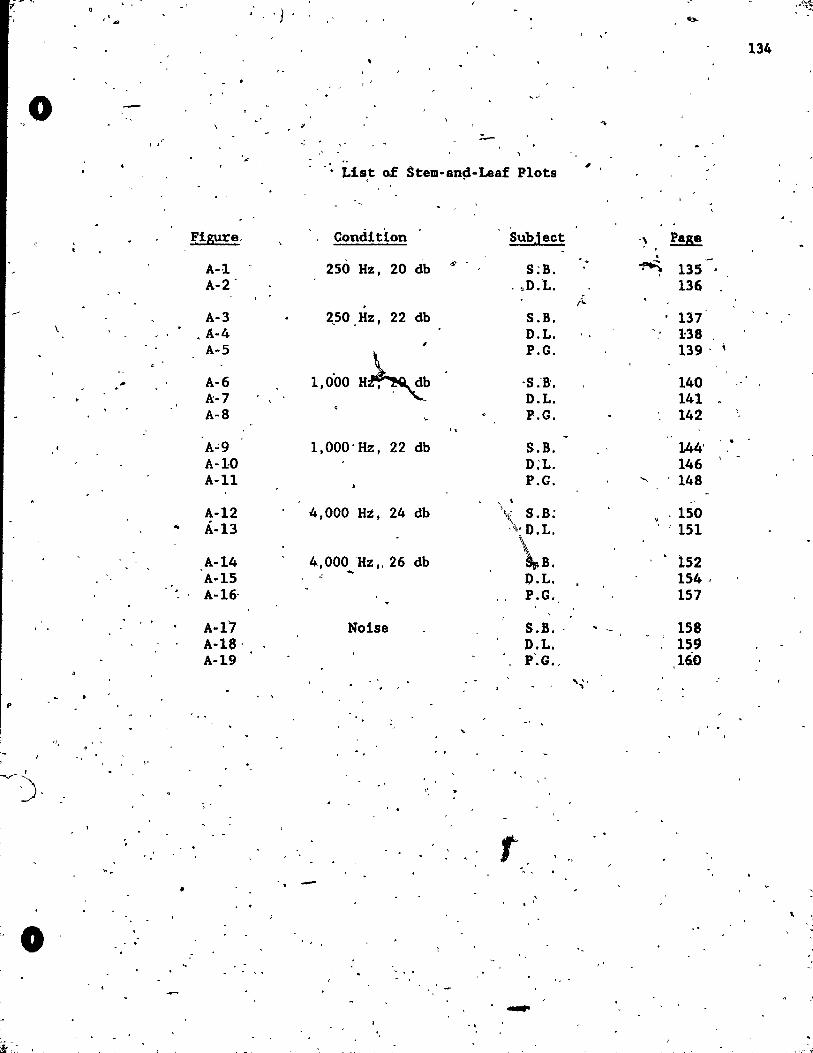
o
p
", r-,
1
~'-)-
0
lt', ~
. 'JO
.
~.
, ,
.-
..
, .
'.
~iS!!re,
A-l A-2 .
A-3 . A-4
A-5
A-6 A-7 A-8
A.i.9 A-lO A-l1
A-12 A-13
A-14 A-l5 A-l6'
A-t7 A-l8 ' A-l9
•
:
, , -
.: . "
': List of Stem-and-Leaf Plots , .
Condition Subject
250 Hz, 20 db e!l ' S;B. .• D.t.
. 2.50.Hz, 22 db S.B.
D.L . , P.G.
H~ 1,0'00 -S:B'. D.L. P.G.
" l,OOO'Hz, 22 db S.B.
D,'L. P.G.
4,000 Hz, 24 db \ 1
\( S.B: ''\.·D L
\' 4,000 Hz" 26 db B . .... p. L. P.G.
Noise S.B. ' D.L. P:G . .
. "
" . , .
f . ,
"
' . - , .
.-. " "
134
" Page . -'+
~ 135 . , 136
lit..
137 ' . 1:38
139 ' , 140 141 142 "
144' ' .
146 \ -
.... 148
.150 ., ' 151
. 152 154, 157
158 159 160
, " é '\
l' .
~
... " :
.' "
'.-.'t
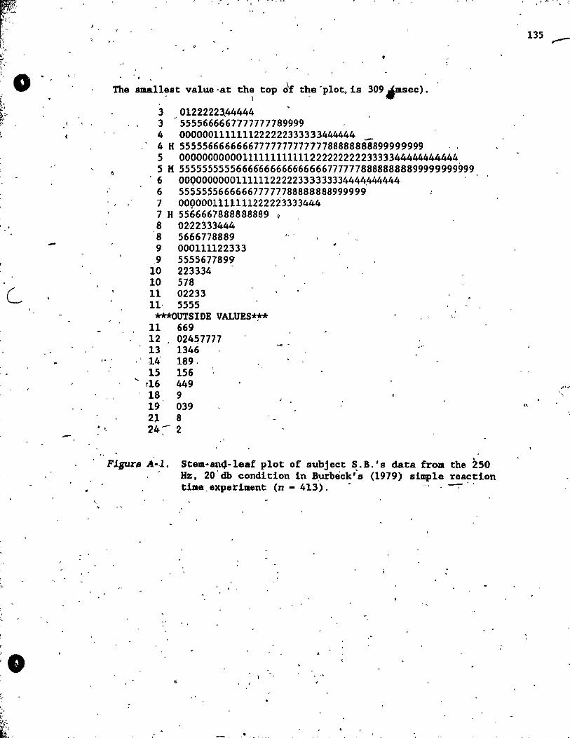
r:tjf;·
~/~I~ ~\ ' , ",
( ,', ,1." \ ). > '
o \ 0
-
. \
" ,
" . ,
The ama11~8t va1ue'at th~ top df the'plot.is 309Atmsec).
3 0122222144444 3 -5555666667777777789999 4 0000001111111222222333333444444 4 H 5555566666666777777777777788888888899999999 ' , 5 0000000000011111111111122222222223333344444444444 5 K 55555555556666666666&6666677777788888888899999999999
. 6 00Q00000001111112222233333333444~444444 6 555555566666677777788888888999999 7 0090001111111222223333444 7 H 5566667888888889 8 02·22333444 8 5666778889 9 000111122333 ,9 5555677899
10 223334 10 57'8 Il 02233 Il, 5555
***OUTSIDE VALUES~ Il 669 12 024~7777 13 1346 14 189, 15 156
... (16 449 18 9 19 039 21 8 24;- 2
~ ,
<,
Figure A-l. Stem-an4-1eaf plot of subject S.B.'s data from the 250 Hz. 20' db condition in B,urbeck"s (1979) simple reaction time, experiment (n - 413). --; " ,
. , , ,
, "
"
.-
135 ,--
1.
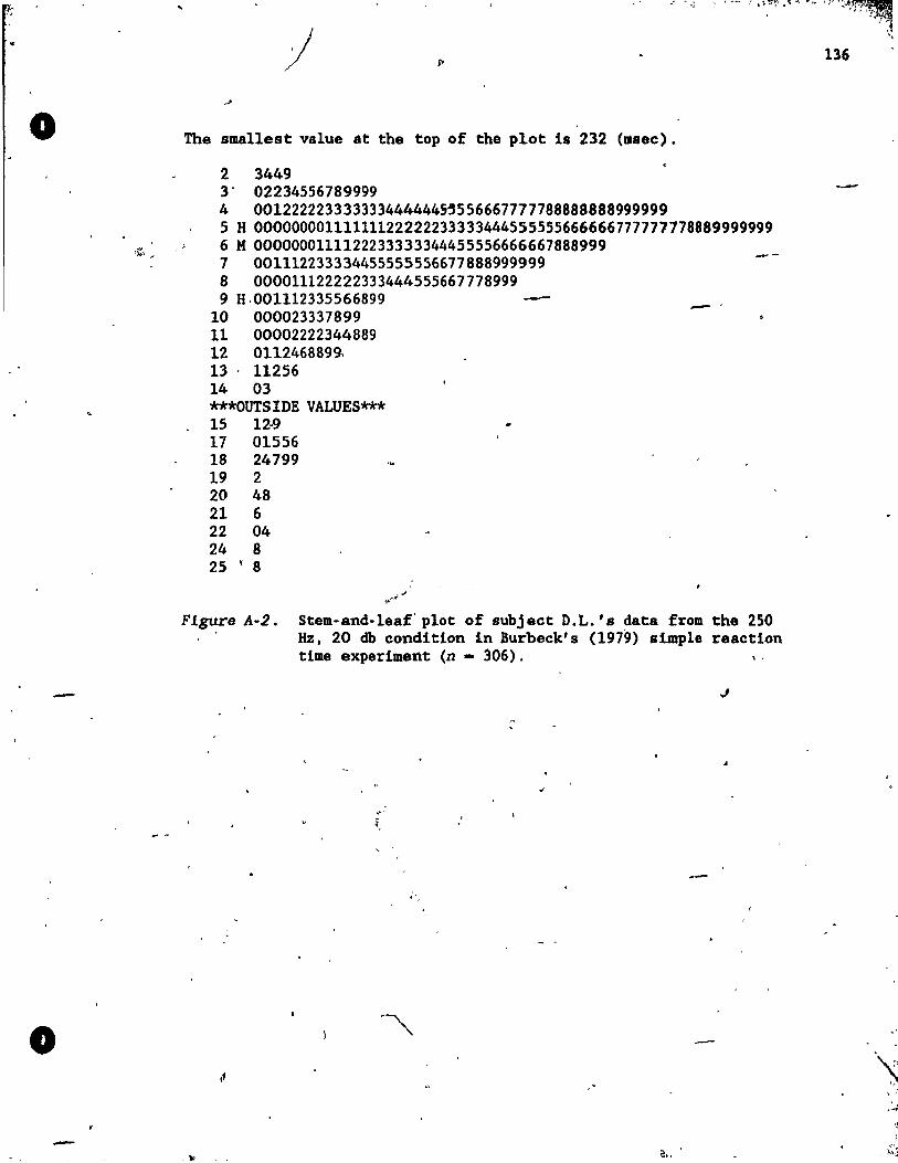
o
-
o
-
...
)
The smallest value 8.t the top of the plot is 232 (Dlsec).
2 3449 3° 02234556789999 4 001222223333333444444~556667777788888888999999 5 H 00000000111111122222233333444555555666666777777778889999999 6 M 0000000111122233333344455556666667888999 7 001112233334455555556677888999999 8 000011122222333444555667778999 9 H,OOl112335566899
10 000023337899 Il 00002222344889 12 0112468899. 13 ' 11256 14 03 ***OUTS1DE VALUES*** 15 12-9 17 01556 18 24799 19 2 20 48 21 6 22 04 24 8 25 1 8
--
-'
FIgure A-2. Stem-and-leaf'plot of subject D.L.'s data from the 250 Hz, 20 db condition in Burbeck's (1979) simple reaction Ume experiment (n - 306). , .
J
~,
~,
136
"
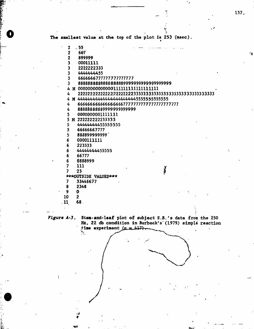
.-
"
. "
/
'(
f
"f, .'
The _ma11est value at the top of the plot 18 25~ (msec) . •
2 .55 2 66'i 2 899999 3 00011111 3 2222222333 3 4444444455 3 6666666777777777777777 3 8888888888888888889999999999999999999 4 H 00000000000000l111111111111111l1
, '"
4 22222222222222~222222233333333333333333333333333333333 4 M 444444444444444444444445555555555555 4 6666666666666666667777777777777777777777 4 88888888889999999999999 5 0000000001111111 5 H 222222222233333 5 44444444455555555 5 66666667777 5 888899999999" 6 0000111111 6 223333 6 44444444455555 6 66777 6 8888999 7 111 7 23 ***OUTSIDE VAWES*** 7 33446677 8 2348 9 0
10 2 .11 68, ,
'1 FJ.gure A-3. Stell-and-leaf plot of subjeçt S.B.' s data fram the 250
Hz, 22 db condition in Burbeck's" (1979) simp1é reaction , ... tille experiment .1D-..::..~'-t-F=--
" "
, \
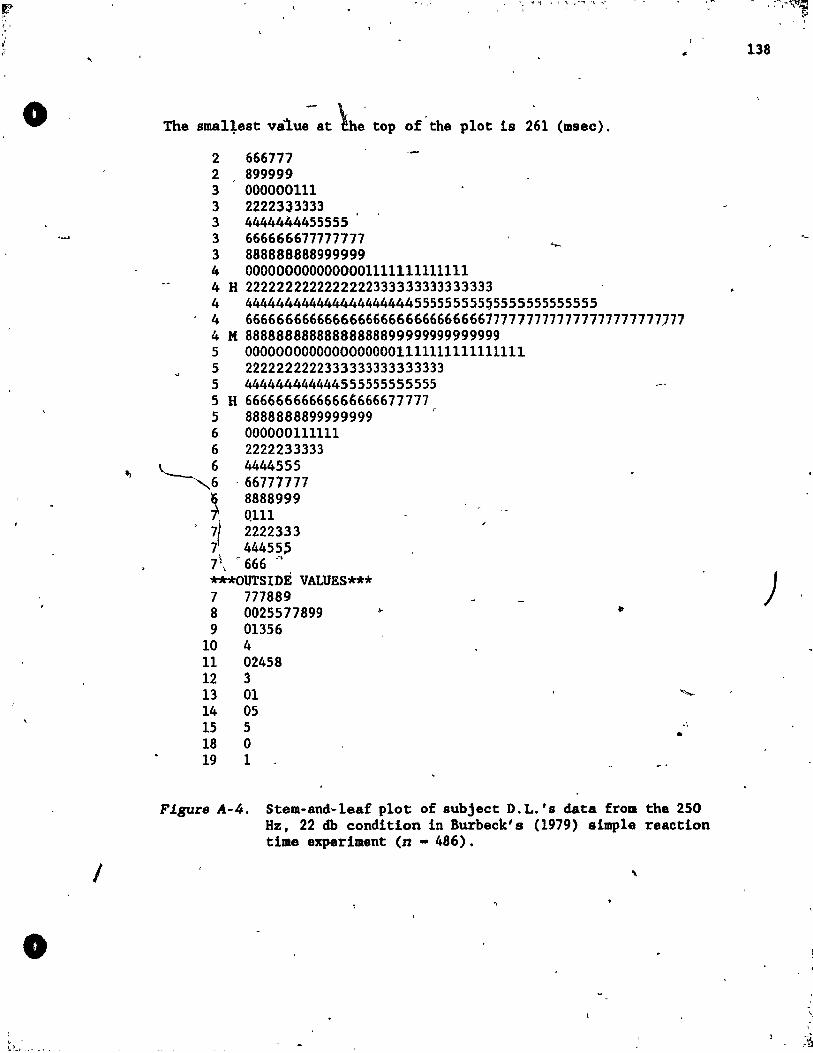
i ,
o
•
.. ~ "
The smallest vaî.u: at \h~ top of the plot is 261 (msec).
2 666777 2 899999 3 000000111 3 22223J3333 3 4444444455555 3 666666677777777 3 888888888999999 4 0000000000000001111111111111 4 H 2222222222222222333333333333333 4 44444444444444444444455555555555555555555555 4 6666666666666666666666666666667777777777777777777777777 4 K 88888888888888888899999999999999 5 00000000000000000001111111111111111 5 2222222222333333333333333 5 444444444444555555555555 5 H 66666666666666666677777 5 8888888899999999 6 000000111111 6 2222233333
'--- 6 4444555 ~6 - 66777777
~ 8888999 -r, Q11l 7{ 2222333 7 44455~ 7\\ r 666 -.... ***OUTSIDE VALUES*** 7 777889 8 0025577899 9 01356
10 4 11 02458 12 3 13 01 14 05 15 5 18 0 19 1
.. •
.\
•
F1gure A-4. Stem-and-leaf plot of aubject D.L.'a data from the 250 Hz, 22 db condition in Burbeck's (1979) simple reaction time experiment (n - 486).
l '
138
)
"
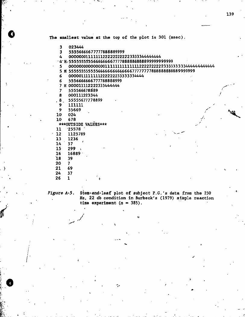
. è
o
)
l, •
1 1
1 1 / '
"'
"-t -...;. .. - "j - ~ .. ,. ~
,
The smal1est value at the top of the plot 18 301 (msec).
3 023444 3 55556666677777888889999 4 00000001111111222222222223333344444444 -~H/5555555S55666666667777888888888899999999999 5 000000000000000111111111111~12222222222333333333444444444444 5 M 555555555555666666666~666677777777888888888889999999 6 0000011111111222222233333334444 6 5556666666777788888999 7 H 000011112222333444444 7 55556'6678889 8 000111223344
. 8 c 55555677778899 9 111111 9 55669
10 024 10 678
***OUTSIDE VALÙES*** Il '25578 ~
'12 1125789 13 1236 14 57 15 299 \ 16 16889 ' 18 39 20 7 21 69 24 37 26 1
, -'..-
f
/
Figure A-5. 1
Stem-and-leaf plot of s$ject P.G.'s data from the 250
/
HZ 1 22 db condition in Burbeck's (1979) simple reaction Ume experiment (n - 385). ~
.~ .'
. ,
....
'.' .
o
139
"
p.
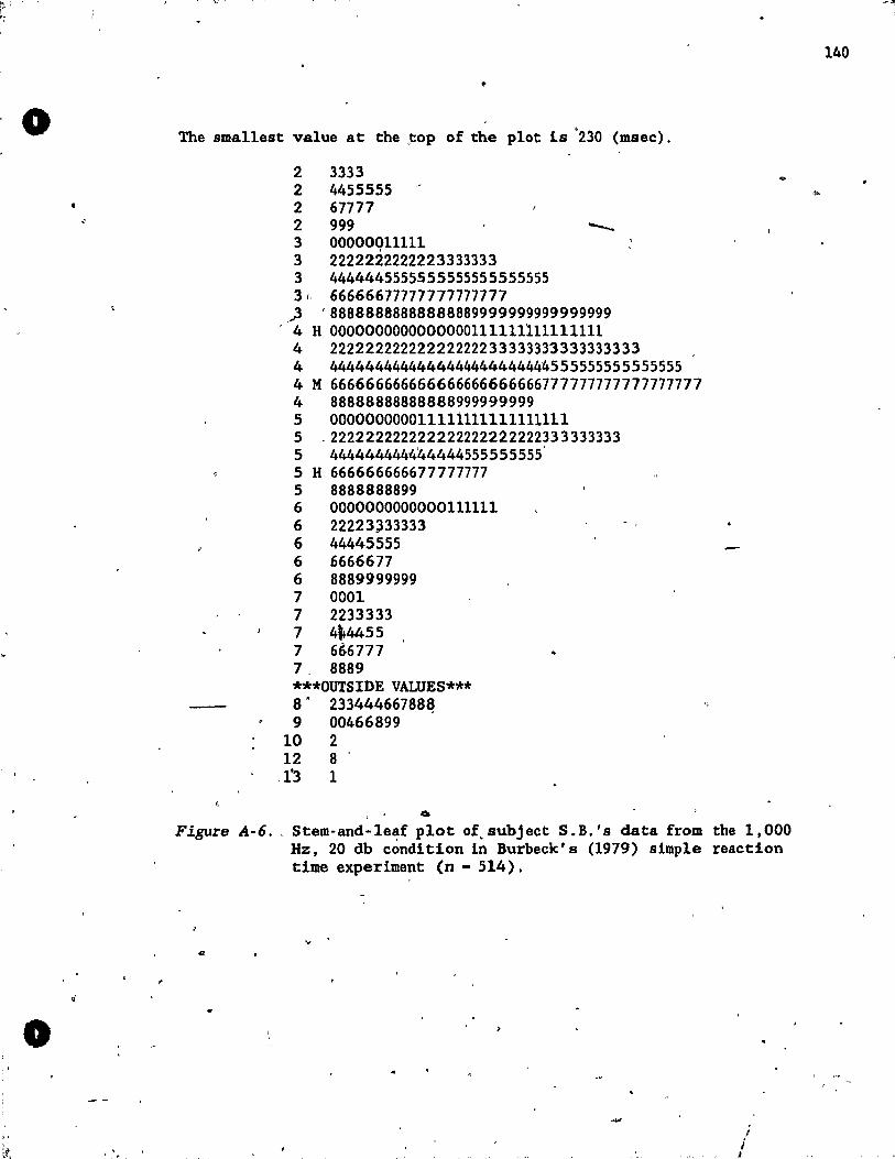
o
. '
o
1 ~ ••
..
The sma11est value at the ,top of the plot ls '230 (msec).
2 3333 2 4455555 2 67777 2 999 __ 3 00000q11111 3 2222222222223333333 3 4444445555555555555555555 3 <. 66666677777777777777
;3 , 88888888888888889999999999999999 4 H 0000000000000000111111111111111 4 22222222222222222233333333333333333 4 4444444444444444444444444555555555555555 4 M 666666666666666666666666777777777777777777 4 88888888888888999999999 5 000000000011111111111111111 5 .222222222222222222222222333333333 5 444444444444444555555555' 5 H 666666666677777777 5 8888888899 6 0000000000000111111 6 22223;n3333 6 44445555 6 6666677 6 8889999999 7 0001 7 2233333 7 4-'4455 7 666777' 7. 8889 ***OUTSIDE VALUES*** 8 • 23344466788~ 4
9 00466899 10 2 12 8
,1'3 1
6
Figure A-6 . . Stem-and-1e~f plot of.subject S.B.'s data from the 1,000 Hz, 20 db condition 1n Burbeck's (1979) simple reaction time experiment (n - 514) •
, Î
1
140
,,,.
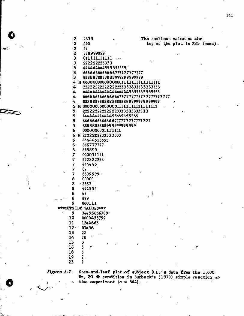
o
\
"
,\
2 2333 The sma11est value at the 2 455 top of ~he plot 1s 225 (lIlsec). 2 67 2 888999999 3 011111111111-3 222222223333 3 444444444555555555 ~ 3 6666666666666777777777177 3 8888888888888999999999999 4 H 00000000000000001111111111111111 4 22222222222222223333-333333333333 4 44444444444444444445555555555555 4 666666666666666777777777777777777777 4 88888888888888888889999999999999 5 M 0000000000000011111111111111111 5 222222222222223333333333333 5 44444444444455555555555 5 6666666666666777777777777777 5 8888888888999999999999 6 0000000001111111 6 H 2222222233333333 6 44444555555 6 666777777 6 888899 7 000011111 7 222222233 7 444445 7 67 7 8899999J 8 00001 8 '2333 8 444555 8 67
__ - '8 899 ? 000111
***OUTSIDE VALUES*** 9 34455666789"
10 0000455799 Il 1244666 12 -- 03456 13 22 14 78
15 ° 16 5 *
18 6 19 2, 23 2
J,
-
Figure A-7. Stelll·and-1eaf plot of subject D.L.'s data frolll the 1,000 Hz, 20 db condition .in Burbeck's (1979) simple reactlon .w
.... time experiment (n - 564). ,. ' '-./ \,
141
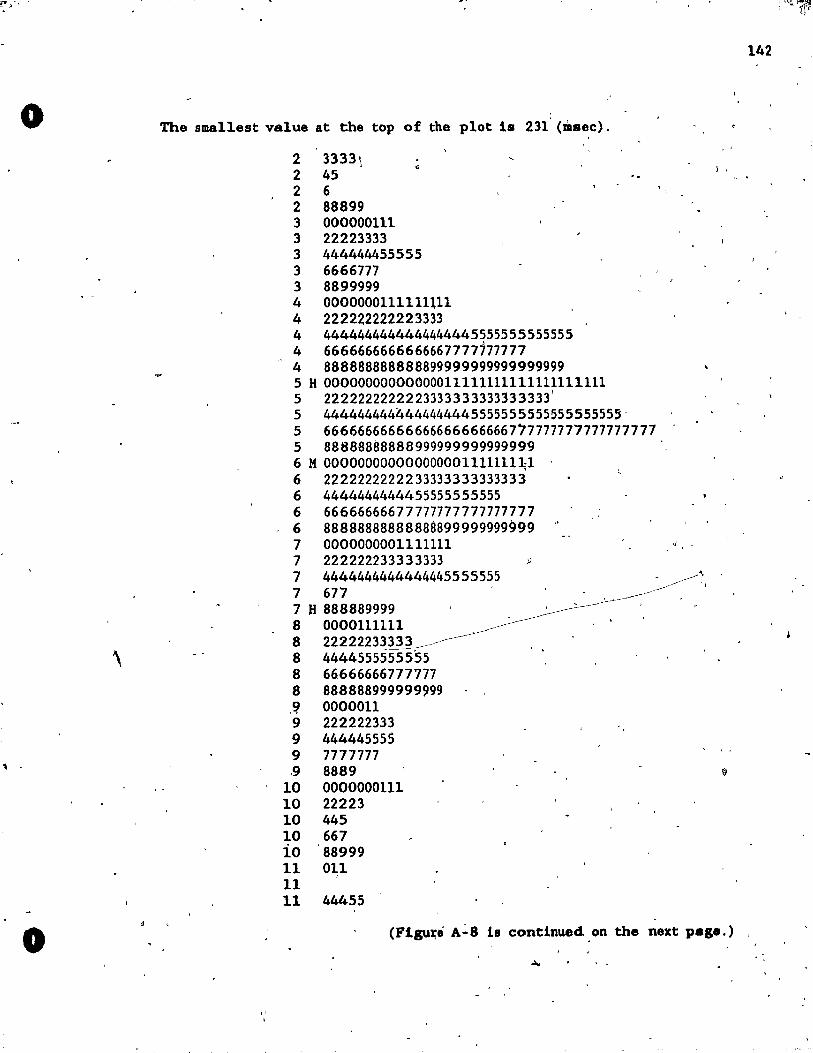
o
\
o
, "
The sma11est value at the top of the plot 18 231' (Daaec).
2 3333\ 2 45 2 6 2 88899 3 000000111 3 22223333 3 444444455555 3 6666777 3 8899999 4 0000000111111111 4 222222222223333 4 4444444444444444445555555555555 4 6666666666666667771'177777 4 888888888888899999999999999999 5 H 00000000000000011111111111111111111 5 2222222222223333333333333333' 5 4444444444444444445555555555555555555 ' 5 66666666666666666666666777777777777777777 5 88888888888999999999999999 6 M 0000000000000000011111111;1 6 2222222222233333333333333 6 4444444444455555555555 6 66666666677777777777777777 6 88888888888888899999999999 7 0000000001111111 7 222222233333333 li
7 4444444444444445555555 7 677 7 H 888889999 8 0000111111 8 22222233333 8 4444555555555 8 66666666777777 8 888888999999999 ,~ 0000011 9 222222333 9 444445555 9 7777777 ,9 8889
10 0000000111 10 22223 10 445 10 667 io 88999 11 011 11 11 44455
,. ;
) ,
(Flgu~é A~8 1& continued on the next page.)
" ,
142
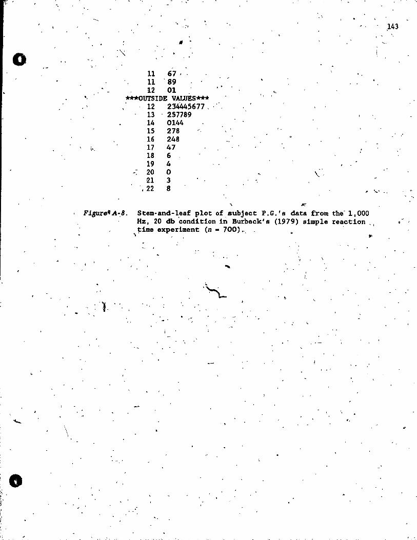
o
\
•
'.
Il •
11 67· 11 '89 12 01 _
***OUTSIDE VAWES*** 12 23444:;677 , 13 257789 14 0144 15 278 ~,
16 248 17 47 18 6 19 4
- 20 0 ,21 3
-,22 8
. ' '.
. ,
-. \.-
F1.gure'A-:8. Stem-and-l,eaf plot of_Bubject P.G.'s data from the'l,OOO Hz, 20 db condition in Burbeck's (1979) simple rea.ction"
.. ~ime exp~rlment (n - 700) ", _ ~ ,.
"
"
"
"
"
"
,143
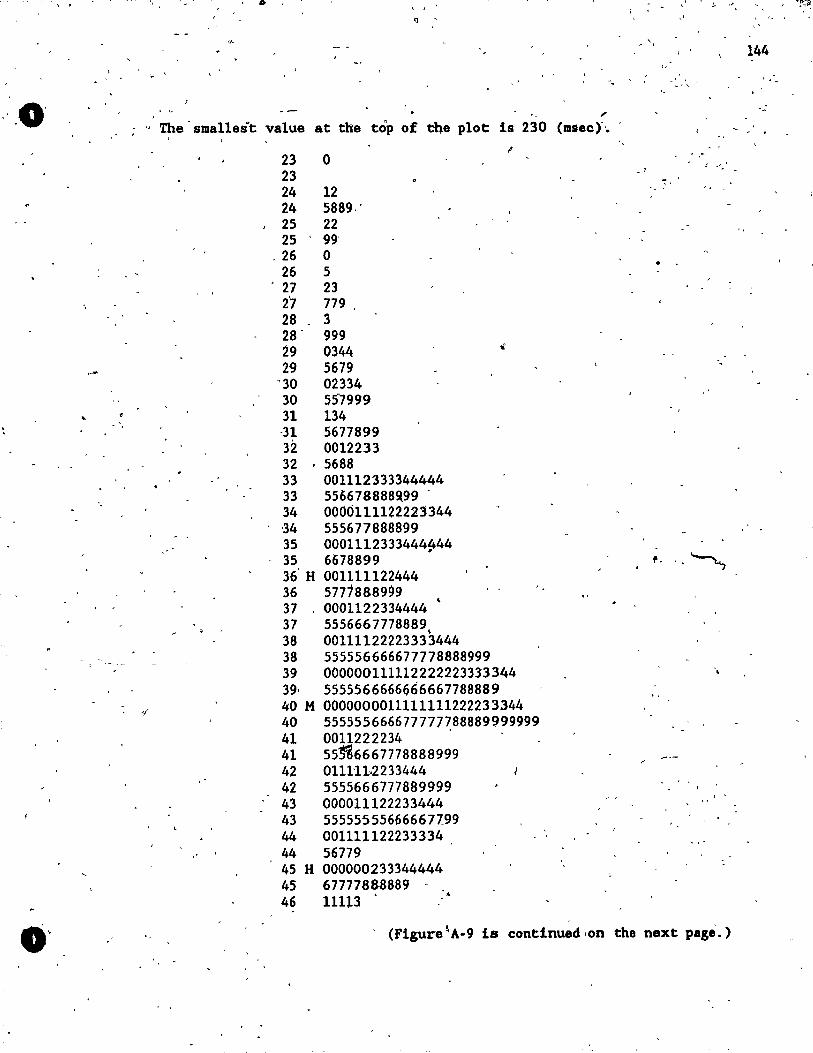
",0'
.. , .. .. ..". . ~ _.- \
q ,
-,
".
" The· smallest value at the top of the plot is 230 (lIIsec)"-. .
"
23 0 23 24 12 24 5889.' 25 22 25 99"
.26 0 26 5
'27 23 2'7 779, 28 3 28· 999 29 0344 29 5679
"30 02334 30 ~S-7999 31 134 ·31 5677899 32 0012233 32 . 5688 33 001112333344444 33 556678888~99· 34 0000111122223344 ,34 555677888899 35 0001112333444;44 35 6678899 36' H 001111122444 36 5777888999 37 ,0001122334444 37 5556667778889, 38 00111122223333444 38 555556666677778888999 39 000000111112222223333344 39, 5555566666666667788889 40 H 0000000011111111222233344 40 555555666677777788889999999 41 0011222234 ' 41 55~6667778888999 42 0111'11.2233444 42 5555666777889999 43 000011122233444 43 55555555666667199 44 001111122233334 44 56779 45 H 000000233344444 45 677778a8889 - . 46 11113 ..
." ~ .... ?,..\ _. f -~ ...
l '
.,
. "
(Flgure~A.9 18 contlnued'on the next page.)
.' 144
, .
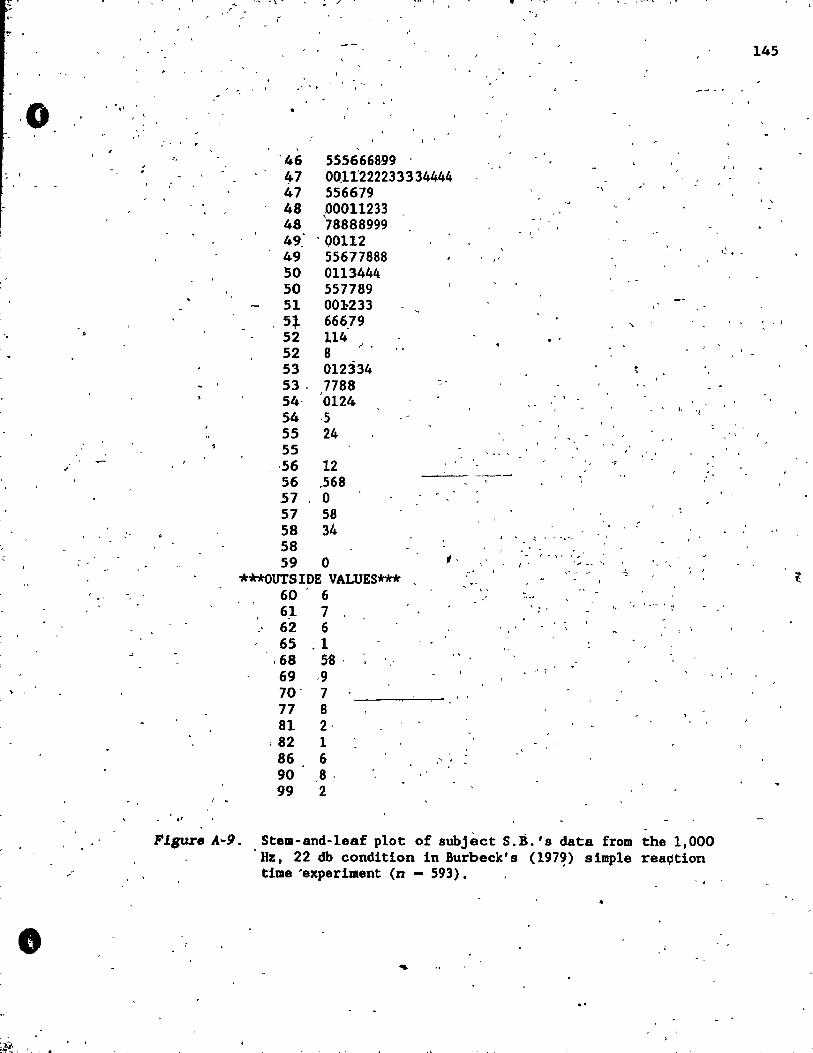
't"'"" .•. ~
..,. .. "'!!. ..... . .... ; •• / •• p •• ... .,... ~ .. ~ ... ~ ... . ····f ·1·:"· : _.~ 1. •
r " " ..
145
, "
' ., .. ' ~ ) . ,0 .'
", "46 555666899 , 1 . 4-7 00.11'222233334444 -
47 556679 "
48 ,00011233 \
48 78888999 49: ' 00112
- ,
1_' •. 49 55677888 "
50 0113444 50 557789 51 00~233
,5:J. 66679 '\ ' ,1
'. ~ 52 114 . ' 52 8
r ,
53 012334 53 ' 7788 , 54· 0124
" 54 ,5 'j
55 24 55 ' ' , ,
~ , ,56 12 .
56 .568 ~,--
57 0 57 58 58 34 :-
~ . - -, ~,
58 0 ;, . f ..... ~ 1 ..
; , 59 , : ' -;a _. "
***OUTSIDE VAWES*** .' , \ ~.. ~. - ~ ,
60 6 --6.1 7 \.; . '.'_ ''i'
62 6 ' .
65 .1 ,68 5'8, ' '
69 ,9 .1 ;
70- 7 77 8 81 ,2,
182 1 86 6 ,~~ j
90 ,8 ' 99 2
1 . . '
, Figure A ... 9. , Stell-and-leaf plot of subjèct S.B.'a data from the 1,000 Hz. 22 db condition in Burbeck' s (197~) simple rea~tion
r Ume 'experiment (n - 593). , . •
• .'
~, '
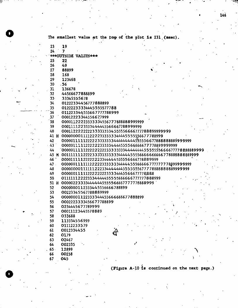
?1""" -
o
, .
o
• 146
The smallest value ~t t~e top of the plot, ls 231 ',(lIsec) •
23 19 24 ' 7
" '***OUTSIDJ!! VALUES*** 25 22 26 49 27 88899 2,8 168 29 123468 30 ,56 31 136678 32 44566677888899 33- 33345555678 34 01222334456777888899 35 01222233334445555577788 36 01122334lt555667777788999 37 0001222334455667..7999 38 00001122223333334556777888888999999 39 0001111223333444445566667788999999 40 0001122222222333333334555556666777788899999999 41 H 0000000011112222333333344445555i,56677788999 \ 42 0000011111222223333333444444444555556677888888889999999
, 43' 0000011111222222333334444555566666677778899999999 44 '000001111122222222233333333444444445555555666677778888889999 45 M 0011111112222333-333333334444455556666666666 7788S6888QS9999 46' '00001111122222223344444555556666778889999 A
47, 0000001111112222233333334444455566666 77777777~99999999 48 000000001111112223344444445555555677778888888889999999 49 000000~1111222222223333444556667777aa8.8 50 011111122223334444455555666666777777888999 51 H 000002233334444445555566667777778888999 ' 52 0000000112333445556666788899 53 00223345567788889999 54 00000001122333344455666666677888899 55 0002223333456677788899 56 0234445677789999 57 00011123445578889 58 033688 59 113334556999 60 01112233579 61 0012334455 62 0179 63 02467 64 002335
. 65, 12899 66 00258 67 045
i r
1
", , 1 .. -
\
l' _
(Figure A· ~O -ts continued on the next page,)
'"
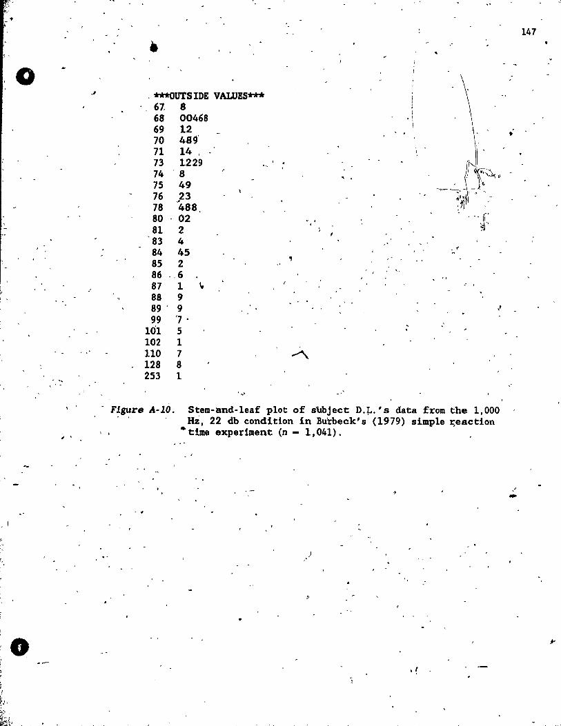
"
o
. '
•
- '. " -
, .
"***OUTSIDE VAWES*** 67, 8 68 00468 69 12 70 489' 71 14, 73 1229 74 '8 7S 49 76 23 78 '488 80 02 81 2 83 4 84 45 85 2 86 -,6 87 1 .. 88 9 89 - 9 99 '7'
1Ô1 S 102 1 110 7 128 8 253 1
...
--,
i ~ !
1
" ..
"
- Figure A-ID. Stem-and-Ieaf plot of aubject D.L.' s data from the 1,000 Hz, 22 db condition in Bu'rbeck's (1979) simple ~eaction
, \ • time experiment (n - 1,041).
- .
•
147 •
, -
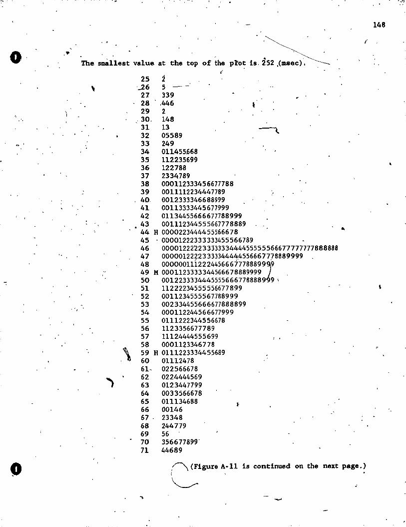
o ,.
"
, "
o
\ -
The smà11est value at the top of the prot Is, 252 .(msec)', 1/
25 2 '..26 5 ~7 339
. 28 . ,446 29 2
,,30, 148 31 13 32 05589 33 249 34 011455668 35 112235699 36 122788 37 2334789 38 000112333456677788 39 0011112234447789 .-40. 0012333346688999 41 00113333445677999 42 01134455666677788999 43 001112344555667778889 44 H 0000223444455566678 45 . 00001222333333455566789 46 00001222223333333444455555566677777777888888 47 00000122223333344444556667778889999 48 0000001li2224456667'7788899
J9
49 H 0001123333344566678889999 50 00122333344455556667788889 9 \ 51 11222234555556677899 52 0011234555567788999 53 002334455666677888899 54 000112244566677999 55 0111222344556678 56 1123356677789 57 11124444555699 , ,
58 0001123346778
,\ 59 H 0111223334455689 60 01112478 61- 022566678 62 0224444569 63 0123447799 64 0033566678 65 011134688 66 00146 67, 23348 68 244779 69 56 70 356677899' 71 44689
Î
,~ (Figure A-11 1s continued on the next page.)
148
,
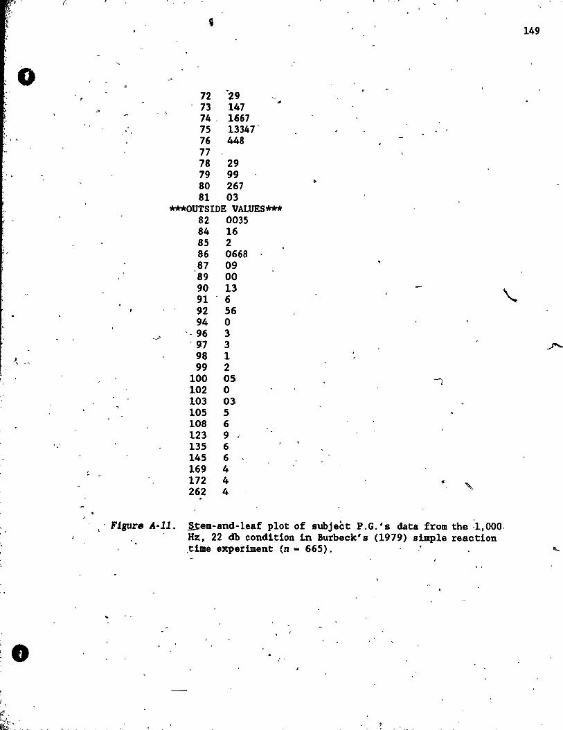
0
, '\ l , ,
;.
) , ~ "
.:
• i.
, "-
72 "29 73 147
.. ,0 , \
74 . 1667 . 75 13347' . '
76 448 77 78 29 79 99 80 267 81 03
***OUTSIDE VALUES***
-Y
\ - Figure A-ll.
82 0035 84 16 85 2 86 0668 87 09 89 00 90 13 91 6 92 56 94 0
',96 3 . 97 3
98 1 99 2
100 05 102 0 103 03 105 5 108 6 123 9 135 6 145 6 169 4 172 4 262 4
.!t;em-and-leaf plot of subject P .G.' s data from the :1,000. Hz, 22 db condition 1n Burbeek's (1979) simple reaction ,time experiment (n - 665) .
" .
. ~ .. ,
149
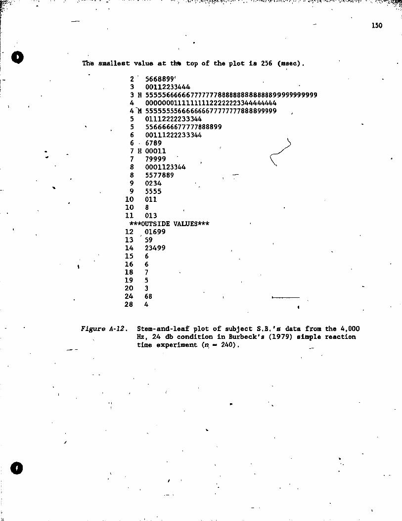
f'
o
·'~I~ :~ ..... \.'\.:,. ... ,~ ,;-~': .. !~~.:;..fi~: .. ï~l"~~;-· ,..".~. : .. 'ït'~·~""(rVf ~:"~~""··r·;l!·~ (-"y .. ~?''I'!,'l')4.t~.yj(~~!;lI.J'':)~l~iiV'"~·''''''''''J'~,~· ~:::tW,!~
The smallest value at tl"$ top of the plot is 256 (msec).
2' 5668899 1
3 00112233444 3 H 555556666667777777888888888888a899999999999 4 000000011111111122222223344444444 4"M 555555556666666677777777888899999 5 01112222233344 5 5566666677777888899 6 00111222233344
6 6789 ! 7 H 00011 7 79999 8 0001123344 8 5577889 9 0234 9 5555
10 011 10 8 Il 013
***OUTSIDE VALUES*** 12 01699 13 59 14 23499 15 6 16 6 18 7 19 5 20 3 24 68 28 4
Figure A-12. Stem-and-leaf plot of subject S.B.'s data from the 4,000 Hz, 24 db condition in Burbeck's (1979) simple reaction time experiment (~- 240) .
..
<"
150
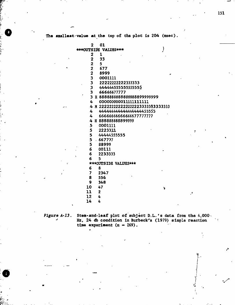
,. , , .
JI
The smalle.t-value at the top of the plot 1s 204 (msee). \..
l'
Figure A-13. .1
•
2 01 ***OUTSlnE VALUES***
2 1 2 33 2 5 2 677 2 8999 3 0001111 3 22222222222333333 ~ 44444455555555555$ 3 66666677777 >
3 H 8888888888888888899999999 4 000000000011111111111 4 M 2222222222222222233333!3333333 4 444444444444444444455555 4 66666666666666677777777 4 H 888888888899999 5 0001111 5 222333.3. 5 44444555555 5 - 667TJ.7 5 88999 6 00111 6 2233333 6 5 ***OUTSIDE VAUJES*** 6 8 7 2347 8 556 9 348
10 47 Il 2 12 4 14 4
Stell-and-leaf plot of"subjéct D.L.'s data from the 4,000, Hz, 24 db condition in Burbeck"s (1979) simple reaction Ume experiment (n - 269) .
' ..
~.~.,.; ..
151
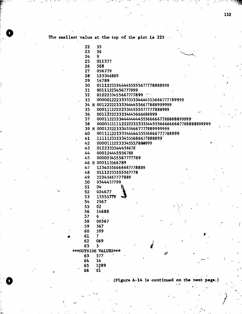
i:',: ...... J: .," \ ...., ~ .. 1
( \
152
0 The smallest value at the top of the _plot 18 225
22 55 23 56 \
24 9 -----...... ,
25 0,11377 26 588 "
27 056779 28 123346889 29 14789 30 011122333444455555677778888999 31 0011122~456777899 32 0122233455667777899 -., 33 000001222333333334444555666777789999 34 H 0012222233334444556677888999999 35 000111122223344555577777888999 36, 0011~22233134445666688999 37 000112233344444444555666667788888899999 38 00001111112222233333344555666666667788888899999 39 M 000122223334556667777889999999 40 0011112233334444455556666777788899 41 111112333334555666677888899 42 0000111223334555}883999 ~
43 0122333344456678 44 000124445556788 45 000023455567777789 46 H 000113566789 47 12345556666667778889 48 01112233555567778 49 22345667777889 ,50 0344457199 51 04
~ 'e 52 024677 53 13355"'" 54 2567 55 02 t \.
, 56 14688 57 6 0
58 ' 00367 . 59 567 . 60 599
,;; 61 7 • 62 069 J
'Jo
63 3 ***OUTSIDE VALUES*** d 63 577 ,
64 14 \
, -65 1?89 66 '01
'-0 (Figure A-14 is conti'nued, on the next page.)
'; .. ')
" c , . .'
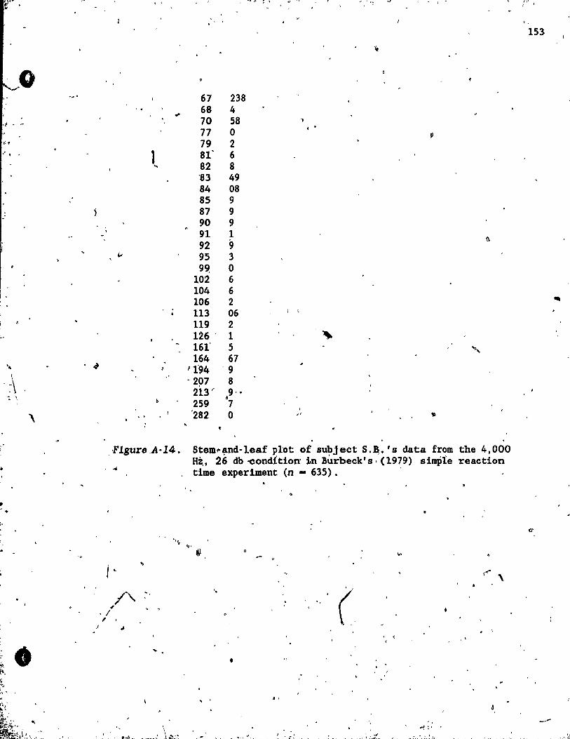
p" •• ' ' ~~ ~ -!.' -1 .. "-.1 -, .. ', ;r .. . .. , '}~--\ ..
153
'ft
0 ~
.~. 67 238
" 68 4
"t .. - 70 58 77 0
/ . Il
lit 79 2 ," . 1 81' 6 .. 82 8
"83 49 84 08 85 9
) 87 9 ,"
90 9 . 91 1
92 9 ~
4- 95 3 99 0
102 6 104 6 106 2 II1II
113 06 : ,
119 2 126 ' 1 ~ 161' 5 ~ ... 164 67
' ... -# ~ 194 '9
'\ . 207 8 21.3 ~ 9, •
':. \ f
259 7 '282
)
\ 0 -' 'III
~
. ,FIgure . .4·14. Stem .. ~nd-leaf plot of Bu~ject S.B,.'8 data from the 4,000 Hz,. 26 db -condition' tn Burbeck' 8' (1979) simPle reaction
0- ~ Ume experlment (n - 635) •
'" ,
" .
1"'- '\
'. ( , <
•
. , " \
~\:... ~ -~~ ~.,,' .. \ ~-~ .. ,..
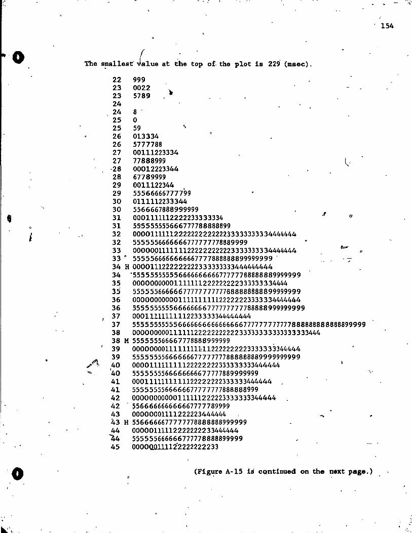
.~
"
• 0
1 .'
.. .-'" 1 ~
" .. ~, -
, 154
The sma11est' L1ue at the top of. the plot ls 229' (msec).
22 999 23 0022 ) 23 5789 24 24 8 ' 25 0 25 59 " 26 013334 26 5777788 27 00111223334 27 77888999 ~,
-28 ' 00012223344 28 67789999 29 0011122344 29 55566666777799 30 0111112233344 30 5566667888999999 31 0001111112222233333334 " >:;
31 55'55'55555666777788888899 32 0000111111222222222222233333333334444444 32 5555556666666777777778889999 33 00000p1111111222222222223333333334444444 &!w
.r>
33" 5555566666666667777888888899999999' --, 34 H 0000111222222222333333333444444444 34 '55555555555666666666677777788888889999999 3~ 00000000001111111222222222333333334444 35 55555566666677777777777888888888899999999 36 00000000000111111111122222223333334444444 36 555555555566666666777777777788888999999999 37 00011111111112233333344444444 37 555555555556666666666666666777777777777888888888888899999 38 00000000011111122222222222333'33333333333333444 38 M 5555555&6667778888999999 39 00000000111111111112222222223333333344444
...... ~\ 39 55555555666666677777777888888889999999999 40 000011111111122222222333333333444444
1 .,. 40 5555555566666666677777889999999 -~I •
41 0001111111111122222222333333444444 41 5555555566666677777777888888999 42 00000000000111111222223333333344444 42 ' 556666666666667777789999 43 00000001111222223444444 , "T
43 H 5566666677777778888888999999 44 00000111112222222233444444 44 555555666666777778888899999 45 000000111122222222233
(Fig~re A-15 18 cQntinued on the next page.)
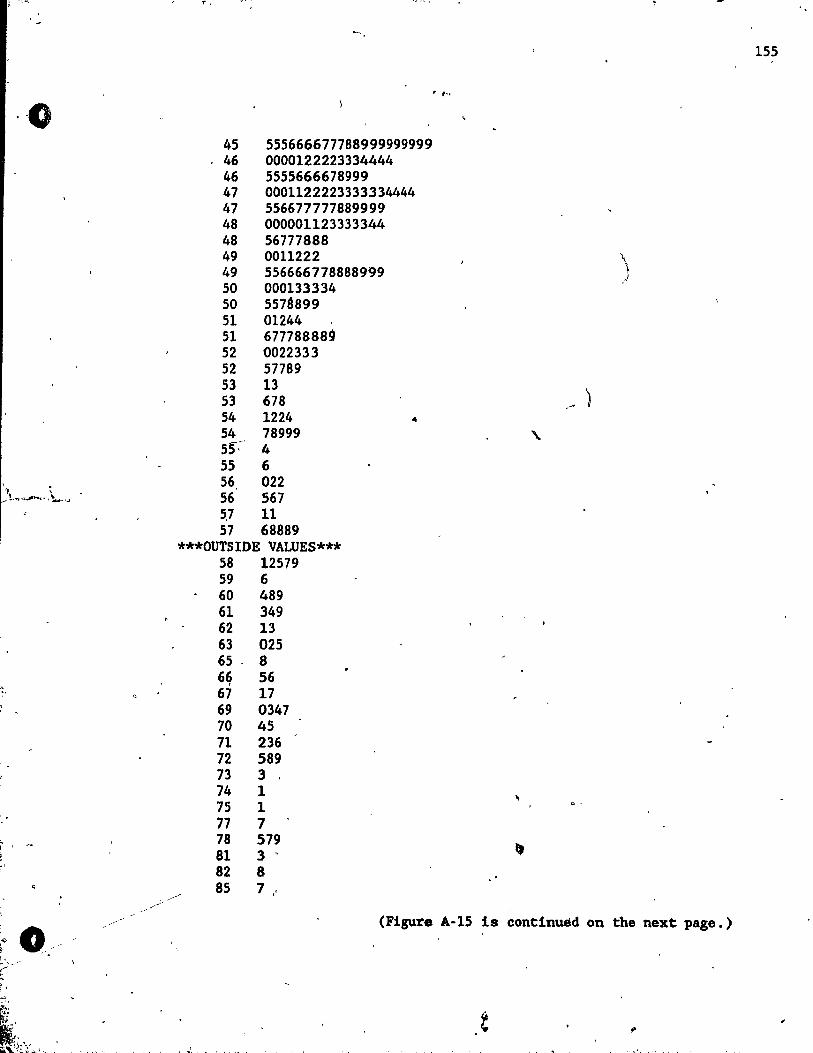
·,0
, . ~\~~·,\...-v .
, . " , ' i
~ 0 .. / '. ,~ ~ _..-
( " ; . ~
~ I,;~ ... , . "'''"''-''~ ,
""'f.
45 555666677788999999999 46 0000122223334444 46 5555666678999 47 0001122223333334444 47 556677777889999 48 000001123333344 48 56777888 49 0011222 49 556666778888999 50 000133334 50 557é899 51 01244 51 677788889 52 0022333 52 57789 53 13 53 678 54 1224 • 54 78999 55:' 4 55 6 56, 022 56 567 5} 11 57 68889
***OUTSIDE VALUES*** 58 12579 59 6 60 489 61 349 62 13 63 025 65" 8 6~ 56 67 17 69 0347 70 45 71 236 72 589 73 3 74 1 75 1 77 7 78 579 81 3' 82 8 85 7"
",:,""
, ,~.
\ )
(Figure A-15 is continued on the next page.)
155
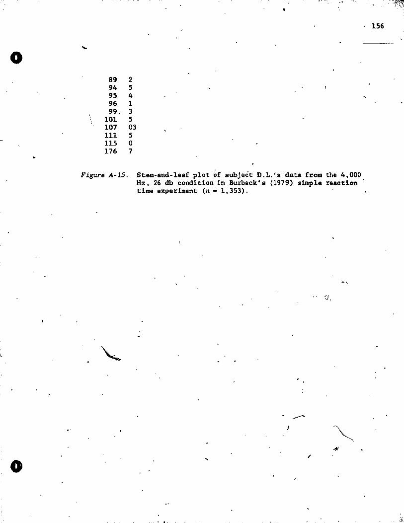
o
..
o
\
89 2 94 5 95 4 96 1 99. 3
101 5 107 03 111 5
115 ° 176 7
.1l';:-.........
Figure A-1S. Stem-and-leaf plot ~f subject D.L.'8 data from the 4,000 Hz, 26 db condition in Bu~beck'8 (1979) simple reaction time experiment (n - 1,353).
~:i ,
. .-'"
.... /
156
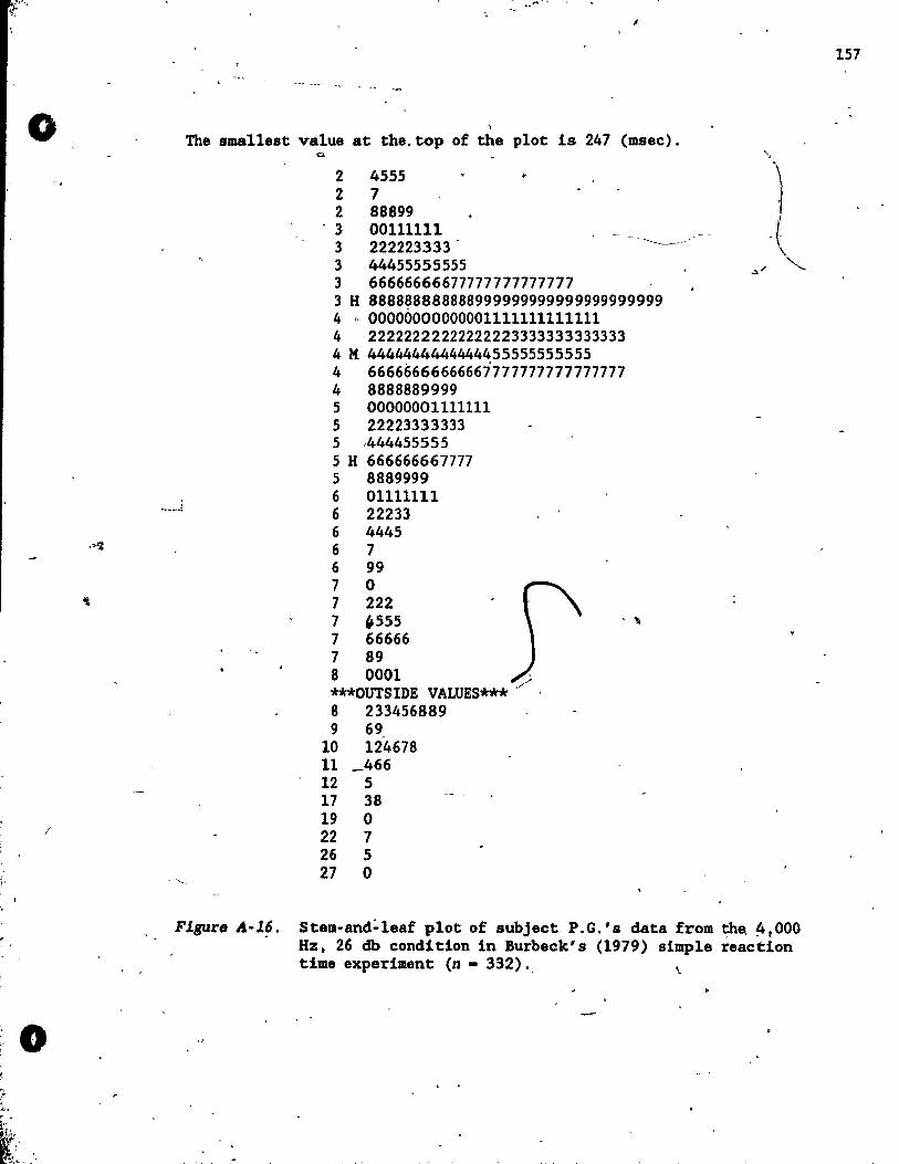
o
·>if
/
o -, r i~ i, .
['
. -... ,<'J.. •••
~. .:~ ;";")~. - ,
--,
, The smal1est value at the. top of the plot is 247 (msec).
._-_..i
- '-.
co
2 4555 2 7 2 88899
- 3 00111111 3 222223333 3 44455555555
..
3 66666666677777777777777 3 H 8888~8888888999999999999999999999 4 " 00000000000001111111111111 4 22222222222222223333333333333 4 M 4444444444444455555555555 4 66666666666667777777777777777 4 8888889999 5 00000001111111 5 22223333333 5 ,444455555 5 H 666666667777 5 8889999 6 01111111 6 22233 6 4445 6 7 6 99 7 0 7 222 7 ,555 7 66666 7 89 8 0001 ; ***OUTSIDE VALUES*** ,/ 8 233456889 9 69.
10 124678 11 _466 12 5 17 38 19 0 22 7 26 5 27 0
. ,
FIgure A-l§. Stem-and:'leaf plot of subject P.G.'s data from ~e, ~,OOO Hz, 26 db condition in Burbeck's (1979) simple reactlon time experiment (n - 332)., \.
157
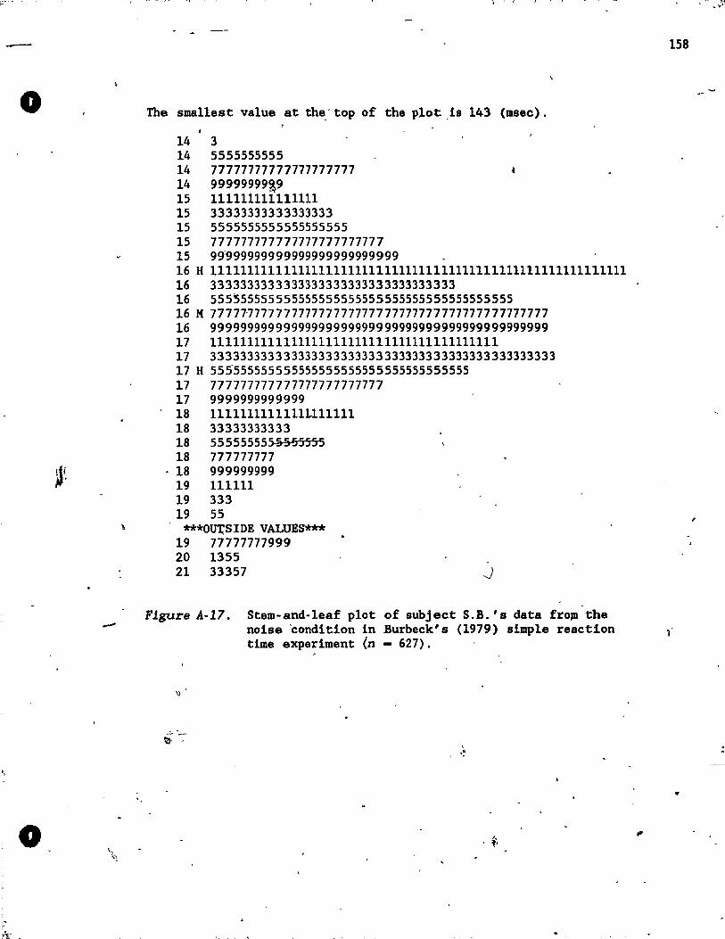
o
\
-
o
, "f· ~ ..• r' ~.> ---r-
The smallest value at the,' top of the plot ,is 143 (msec).
14 3 14 5555555555 14 77777777777777777777 ~
14 99999999~9 15 111111111111111 15 33333333333333333 15 5555555555555555555 15 777777777777777777777777 15 99'999999999999999999999999 16 H 1111111111111111111111111111111111111111111111111111111111 16 3333333333333333333333333333333333 16 555~55555555555555555555555555555555555555 16 H 77777'177777777777777777777777777777777777777777 16 99999999999999999999999999999999999999999999999 17 1111111111111111111111111111111111111111 17 333333333333333333333333333333333333333333333333 17 H 555555555555555555555555555555555555 17 777777777777777777777777 17 9999999999999 18 11111111111111111111 18 33333333333 18 5555555555555555 18 777777777
. 18 999999999 19 111111 19 333 19 55
***Om:SIDE VAWES*** 19 77777777999 20 1355 21 33357 .j
Figure A-17. Stem-and-1eaf plot of subject S.B. ' s data froJll the noise 'condition ln Burbeck' s (1979) simple react10n Ume experiment (n - 627).
\J
, .~
158
,
..
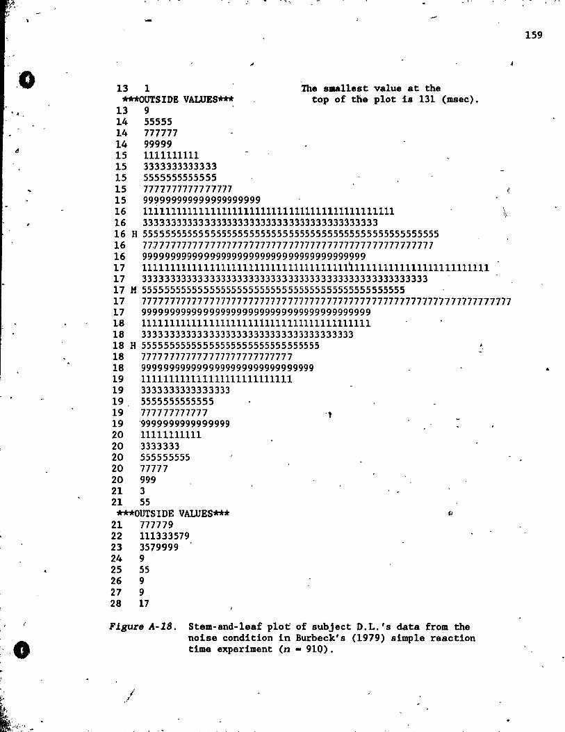
.0 . ~ ,
" ,""" "." .. ~.: ... ; ... \"'"
13 1 The ama11eat value at the ***OUTSIDE VAWES*** top of the plot ia 131 (maec).
13 9 ' 14 55555 14 777777 14 99999 15 1111111111 15 3333333333333 15 5555555555555 15 7777777777777777 15 99~999999999999999999
16 111111111111111111111111111111111111111111111 16 333333333333333333333333333333333333333333 16 H 55555555555555555555555555555555555555555555555555555 16 77,77777777777777777777777777777777777777777777777777 16 9999999999999999999999999999999999999999 17 11111111111111111111111111111111111111111111111111111111111111 17 333333333333333333333333333333333333333333333333333 17 M 55555555555555555555555555555555555555555555555 17 777777777777777777777777777777777777777777777777777777777777777777 17 99999999999999999999999999999999999999999 18 11111111111111111111111111111111111111111 18 33333333333333333333333333333333333333 18 H 55555555555555555555555555555555 18 777777777777777777777777777 18 9999999999999999999999999999999 19 111111111111111111111111111 19 3333333333333333 19 5555555555555 19 777777777777 19 '9999999999999999 20 11111111111 20 3333333 20 555555555 20 77777 20 999 21 3 21 55 ***OUTSIDE VALUES***
21 777779 22 111333579 23 3579999 24 9 25 55 26 9 27 9 28 17
FIgure A-lB. Stem-and-lesf plot of subject D.L.'s data from the noiae condition in Burbeck's (1979) simple reaction time experiment (n - 91Q).
,/
159
•
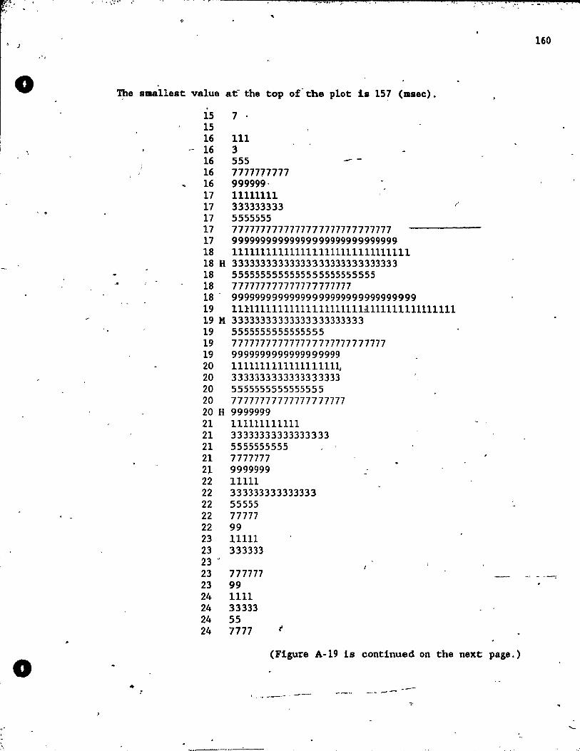
'"f:':'ift-:-~ -- -- -- ---.- -.; -.~": 1·--- .' a, ..... :e;;c; ,~ - " , . ' .. ,4: ~ ,_ "'~":;''' t ",2 ,J., : - .., . :~ .... i >,
.. .. , J 160
,',
0 The sma11est value at the top of' the plot 1s 151 . , ( .. sec) •
15 1 15 16 111
.- 16 3 16 555 .- -16 7711771771 16 999999· 11 11111111 11 333333333 /'
, . 17 5555555 17 7177717777777777777777777777 17 99999999999999999999999999999 18 1111111111111111111111111111111 18 H 33333333333333333333333333333 18 5555555555555555555555555
,0 18 777777777777777777777 18 . 99999999999999999999999999999999 19 11l11111111l11111111111l111111111l11111 19 M 33333333333333333333333 19 5555555555555555 19 777777777777777777777777777 19 9999999999999999999 20 11l111111111111111~ 20 3333333333333333333 20 5555555555555555 20 77777777777777777777 20 H 9999999 21 111111111111 21 33333333333333333 21 5555555555 21 7777777 21 9999999 22 11111 22 333333333333333 22 55555 22 77777 22 99 23 11111 23 333333 23 " 23 777777 _ ... --23 99 24 1111 24 33333 24 55 24 7771
,
0 (Figure A-l9 ls continued on the next page.)
• ( --'" ... --- - -----~
......,--~- -p'" ---
~,
, --, '. -'.
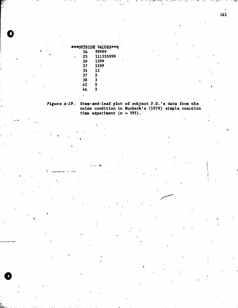
o
• ,t;:L
~k:.".
" .
***OUTSIDE VALUES~
F1.gure ~-19.
l -~
2{. 99999 25 111355-999 26 1399 27 1599 31 13 37 5 38 3 42 5 44 3
Ste~-and-1eaf plot of subject P.G.'s data from the noise condition in Burbeck's (1979) simple reaction time'experiment (n 595).
161
\
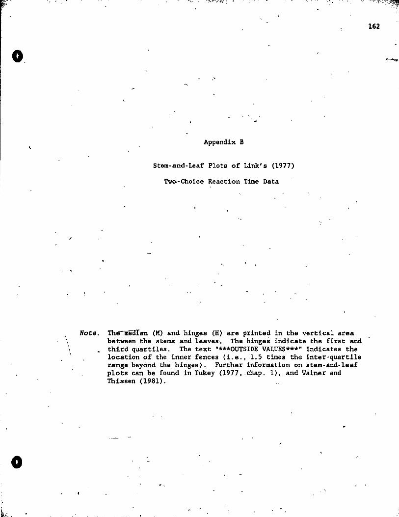
o.
"
\ Note.
..
o
"
-;" , ,~ .. " ." ~ ... r r ;
Appendix B
Stem-and-Leaf Plots of Link's (1977)
Tw~-Choice Reaction Time Data
.'
"
The medIan (M) and hinges (H) are printed in the vertical area between the stems and 1eave~. The hinges indicate the first and third quartiles. The text "***OUTSIDE VALUES***" indicates the location of the inner fences (i.e., 1.5 times the inter-quartile range beyond the hinges). Further information on stem-and-leaf plots can be found in Tukey (1977 •. chap. 1), and Wainer and Thissen (1981).
162
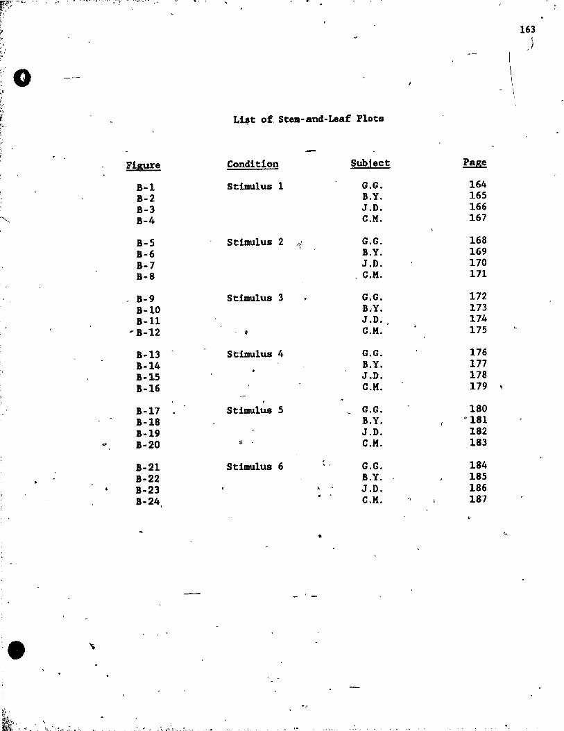
,.~~~ ..... ~'" ,. ',.
"
.'
" 0 .' "C
"
~~~ ~
1.-h 1
"
1
'"""'-
• , . ~ ....... '~.~ .... ; , ....
. ; , .. ";-'
•
...
Figure
B-1 B-2 B-3 B-4
B-5 B-6 B-7 S-8
B-9 B-10 B-11
··B-12
B-13 :&-14 B-15 B-16
B-17 B-18 B-19 B-20
B-21 B-22 B-23 B-24 .
, , '" _.... . '- .. '~ :
"'_",' ," , . ,.~ .. . .. "~--i ,
163 j
- \
L~t of Stem-and-Leaf Plots
Condition Sub1ect Page
Stilll111us 1 G.G. 164 B.Y. 165 J.D. 166 C.M. 167
Stimulus 2 ~~ G.G. 168 B.Y. 169 J.D. 170
' C.M. 171
Stimulus 3 G.G. 172 B .. Y. 173 J .D .• 174
li C.M. 175
Stimulus 4 G.G. 176 B.Y. 177 J.l>. 178 C.M. 179
, Stimulus 5 G.G. 180
B.Y. ·181 J.D. 182
~ C.M. 183
Stimulus 6 . , G.G. 184 B.Y. 185
~ J.D . 186 • C.M . 187
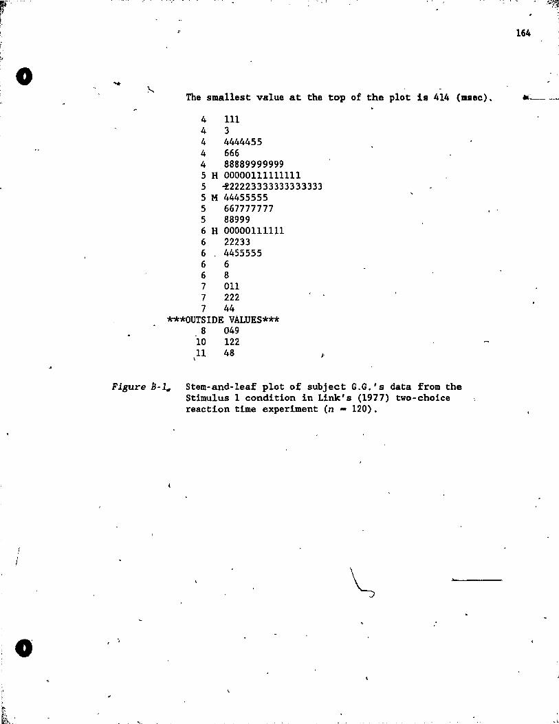
o
•
,. , .... ,
The smallest value at the top of the plot ls 414 (msee).
4 111 4 3 4 4444455 4 666 4 88889999999 5 H 00000111111111 5 ~22223333333333333
5 M 44455555 5 667777777 5 88999 6 H 00000111111 6 22233 6 4455555 6 6 6 8 7 011 7 222 7 44
***OUTSIDE VALUES*** 8 049
10 122 11 48
\
Figure IJ-l" Stem-and-leaf plot of subject G.G.' s data from the Stimulus 1 eo~dition in Link' s (1977) two-choice reaction time experlment (n - 120).
..
:
164
---
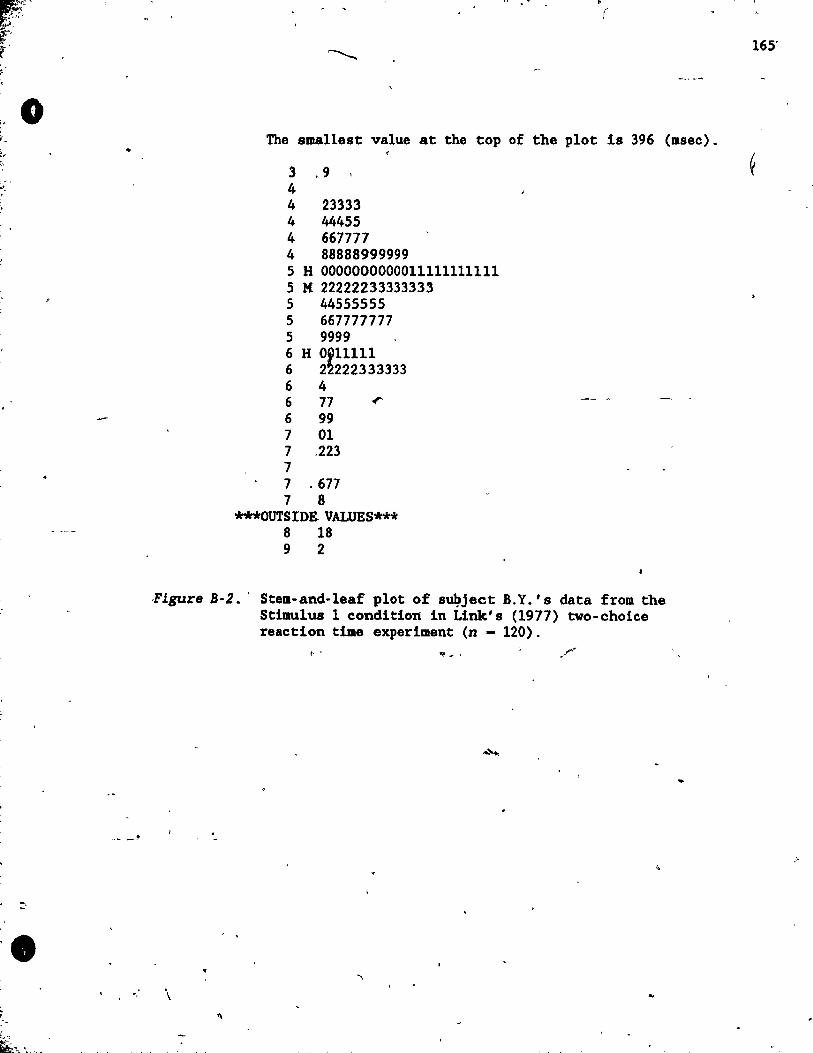
( . , ~"
", ,
,
,
;: .
• C., ti..'t, "
-- -'
.
(
The ama11est value at the top of the plot Is 396 (msee).
3 • 9 4 4 23333 4 44455 4 667777 4 88888999999 5 H 0000000000011111111111 5 M 22222233333333 5 44555555 5 667777777 5 9999 6 H OP11111 6 2~222333333 6 4 6 77 ..r 6 99 7 01 7 .223 7 7 .677 7 8
***OUTSID& VALUES*** 8 18 9 2
.Flgure B-2 • . Stell-and-leaf plot of su1?ject B. Y. ' a data from the Stimulus 1 condition in Link's (1977) two-choiee reaetlon time experiment (n - 120) . . ' "'#'
. - -
'" \
'\
165"
0'
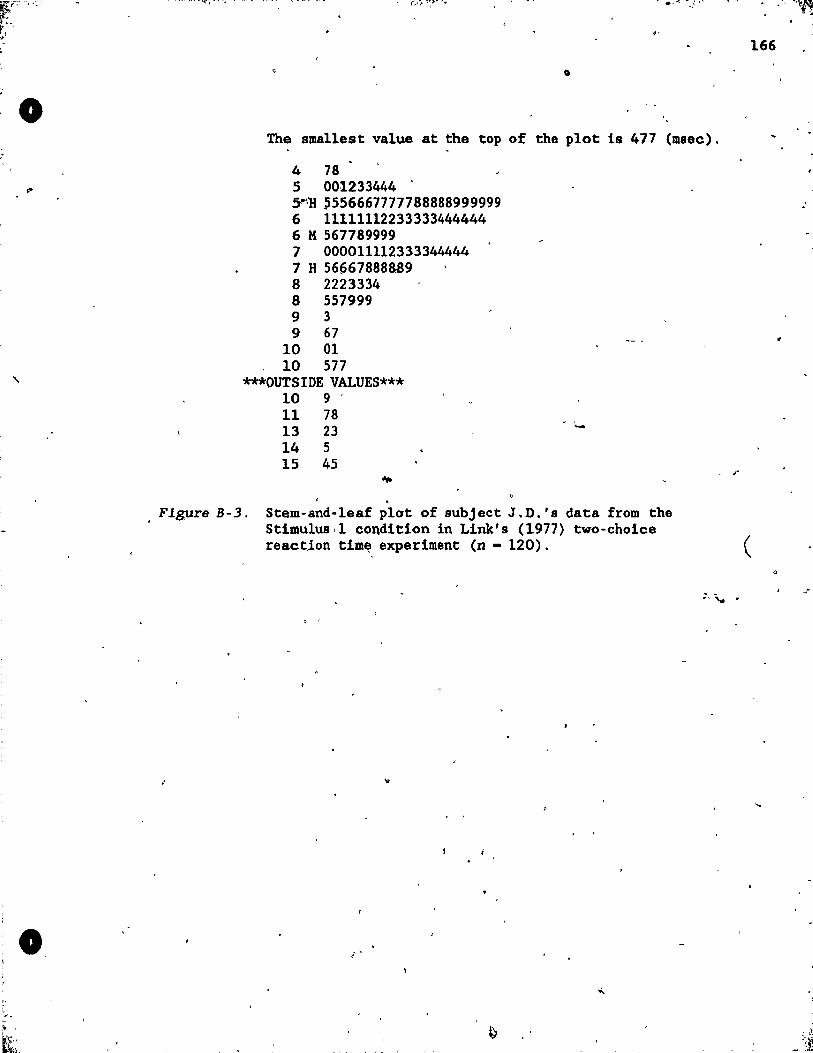
o
o
....... ".\_ ...... -.... ", .~. ,. ,- .','" _~ ". ',··.·'.f~,., •. _\. __ ~f~
.-
The amallest value at the top of the plot ia 477 (msec).
4 78 5 00,1233444 5""''H '556667777788888999999 6 11111112233333444444 6 K 567789999 7 000011112333344444 7 H 56667888&89 8 2223334 8 557999 9 3 9 67
10 01 10 577
***OUTSIDE VALUES*** 10 9-11 78 13 23 14 5 15 45
. , r
. Fl~re B-3. Stem-and-1eaf plot of subject J .D.'a data from the Stimu1us,1 condition in Link's (1977) two-choice reaction tim~ experiment (n - 120). (
, '
166
:
o
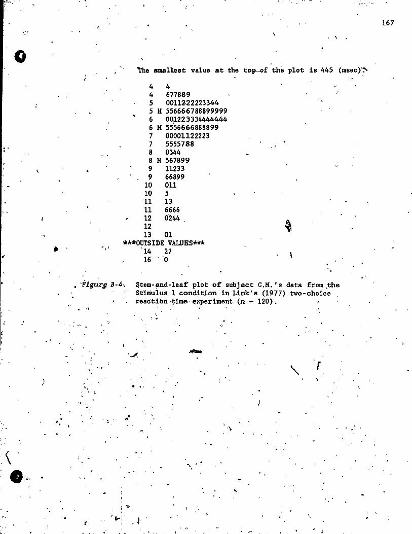
o
,
... . c ,
.....
"
: - ~ . ..'-
.: 1 ..
'.
l'
)
•
"
, •. t·· ... , -- ; ....,. .. '-
. , .
\
"'rhe smallast value at the t~of thè plot is 445 (msec)"":' )
4 4 4 677889 j
5 0011222223344 ? '.,.
5 H 556666788899999 " 6 001223334444444
6 M 5556666888899 7 00001122223 7 5555788 8 0344 8 H 567899 9 11233 9 66899
10 011 10 5 11 13 11 6666 12 0244 12 13 01
***OUTSIDE VALUBS*** ~ ~, 1
14 27 16 "0
\
-FigurA B-4·. ~tem-~nd-leaf plot of subject C.M.' s data from ,the St'iniulus 1 condition in Link' s (1977) two-choice reactibn ·~ime' e,xperiment (n - 120).
, . , , ",. l';'
, .
.'
If
','
..
1 'Il'
, ' ..... i 1
. 1 .
.. ,
lI' l
"
\ ~ .
,
... ,"
a
"
r "
'\
..
\ - \
167
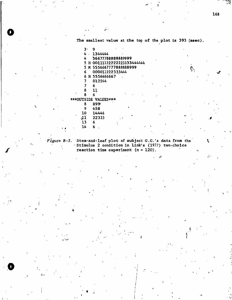
, , 1
o
o
,0
,. .-
.. ~"
The smallest value at the top of the -plot is 393 (msec).
- ,
3- 9 4 ' 1344444 4 '56677788888889999 5 H 00111122222223333444444 5 M 5556667777888888999 6 0000112223~3444 6 H 5556666667 7 012244 ., 6
8 Il 8 6 .
***OUTSIDE VALUES*** 8 89~ . 9 458
10 14446 rJ.l 22333 , . 13 '6 14 6.
,
~, , 1
.,
'Figure B-S. 'Stem-and-1eaf plot of subject G.G.'s data from the' . Stimulus 2 condition in Llnk' s (1977) two~choice reaction time experiment (n. 120).
, .i'
, . 1 , ;
t
, ,
'"
"
168
.p
. .
" 1
jU
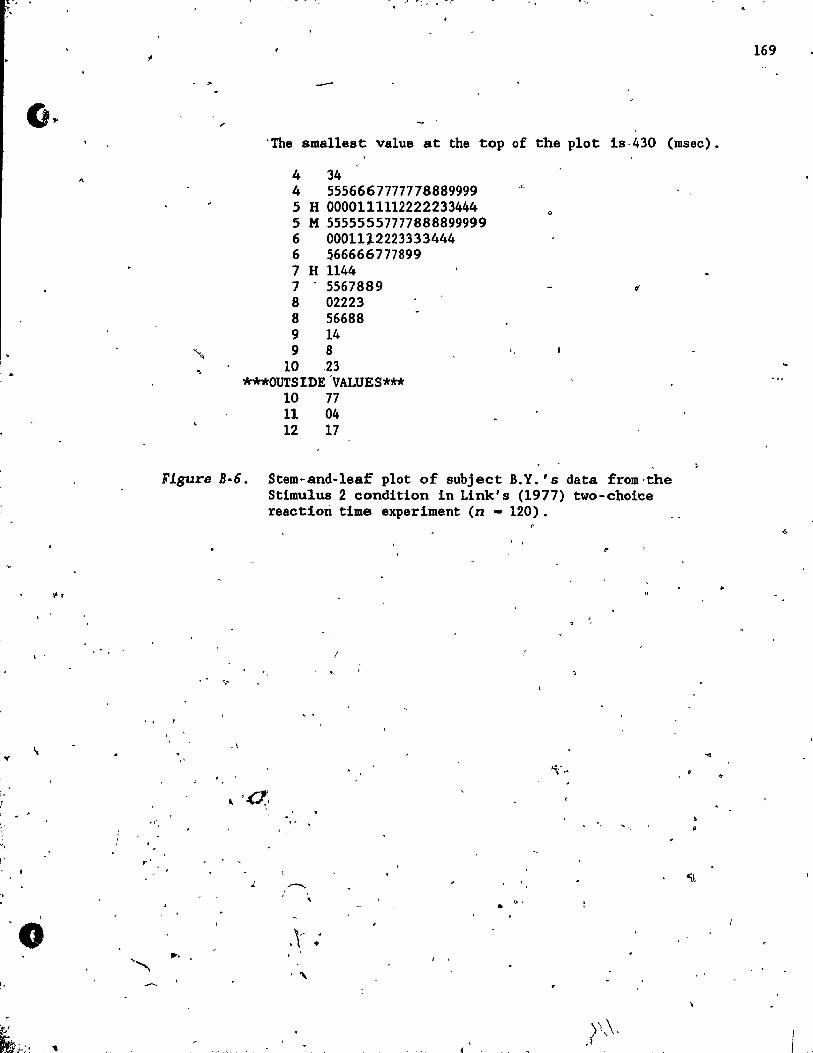
Of
i. f
" l
., i'
, '
'~' " " ~*-.-.
, .
~
r'
,
••• -1 ~
-'The smallest value at the top of the plot 1s -430 (msec).
4 34 4 5556667777778889999 5 H 0000111112222233444 5 M 55555557777888899999 6 0001112223333444 6 566666777899 7 H 1144 7 5567889 8 02223 8 56688 9 14 9 8
10 .23 ***OUTSIDE 'VALUES***
10 77 11 04 12 17
F1gure B-6. Stem-and-leaf plot of subject B.Y.'s data from'the Stimulus 2 condition in Link' s (1977) two-choi'Ce reactiori time experiment (n - 120) .
.\
.>
"
,.---.. , ,
,~ . , \ . ''\.
/
•
J , .
"
169
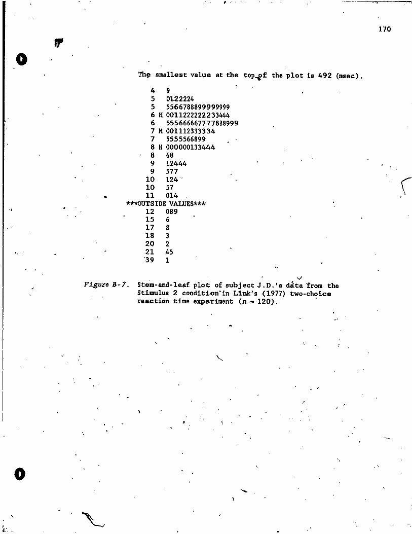
o
. ' , ,
o
..
..
, », -,
Th~ smallest value at the top-ef the plot is 492 (msec),
4 9 5 0122224 5 5566788899999999 6 H 0011222222233444 6 555666667777888999 7 M 001112333334 7 5555566899 8 H 000000133444 8 68 9 12444 9 577
10 124 ~ 10 57 11 014 ,
***OUTSIDE VALUES*** 12 089 15 6 17 8 18 3 20 2 21 45 ~39 1
v Figure B-7. Stem-and-1eaf plot of subj ect J . D, ' s d~ta 'frol1l the
Stimulus 2 condition'in L1nk' s (1977) two-choice reaction time experiment (n - 120), ' .
..
" '
'.
" k~
170
( .
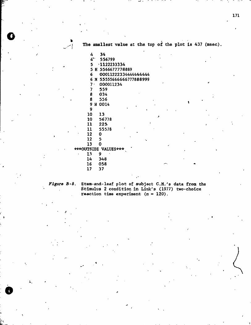
;'
"
. ,. e r
~
o "
. •
. i. ~ . _ -i. .. ~ •• ~ 'I v • .,. .... 1.. , .. ~ i' 'J" .. '.: _..... fI" _. '1,
171
The smallest value at the top of the plot is 437 (msec).
4 34 4- 556799 5 -1122233334 5 H 5566677778889 6 00011222334444444444 6 H 55555666666777888999 7' 000011234 7 559 8 034 8 556 9 H 0014 9
10 10 11 11 12 12 13
13 56778 22~ 55578 o 5 o
***OUTSIDE VALUES*** 1) 9 14 348 16 058 17 37
FIgure B-B. ~tem-and-leaf plot of subject C.H.'s data from the Stimulus 2 condition in Link' s (1977) two-choice reaction time exper:1ment (n - 120).
,f
..
, ,
c
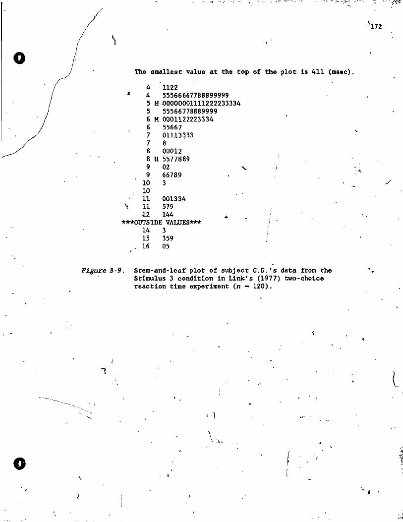
o
-----.---
o 0,
-.,. ,.., :"" r;r-.Jt" ~_ .. --~ ': .. "-, ~ ~~è~ <\
The sma11est value at the top of the plot is 411 (msec),
a 4 1122 4 55566667788899999 5 H~0000001111222233334 5 55566778889999 6 M 0001122223334 6 55667 7 01113~33
7 8 8 00012 8 H 5577889 9 02 9 66789
10 3 10 11 11 12
001334 579 144
***OUTSIDE VALUES*** 14 3 15 359 16 05
1 1
1 1
Figure B-9. Stem-and-leaf plot of subject G.G.'s data from the Stimulus 3 condition in Link's (1977) two-choice reaction time experiment (n - 120).
, , ,
. ,
)
" , , "
.. ' , .,
./
l
\'; .
", ".li
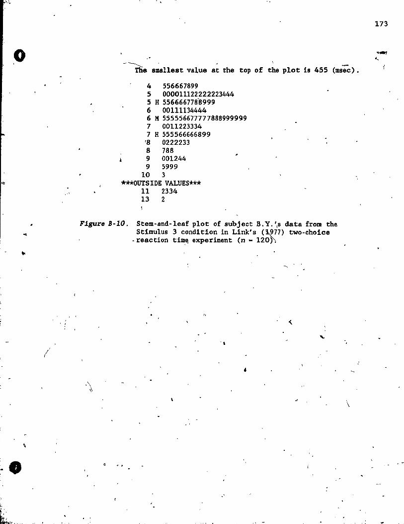
o
,
-.
~- ' ---The ama11est value at the top of the plot is 455 (msec).
4 556667899 5 000011122222223444 5 H 5566667788999 6 00111134444 6 K 555556677777888999999 7 0011223334 7 H 555566666899
'8 0222233 8 788
k 9 001244 9 5999
10 3 ***OUTS IDE VALUES***
11 2334 13 2
F1gure B-IO. Stem-and-1eaf plot of subject B.Y. '\s data from the Stimulus 3 condition in Link's (~977) two-choice
. reaction tim,e. experiment (n - l20h
/,
'!
o c ..
, f
, \
173
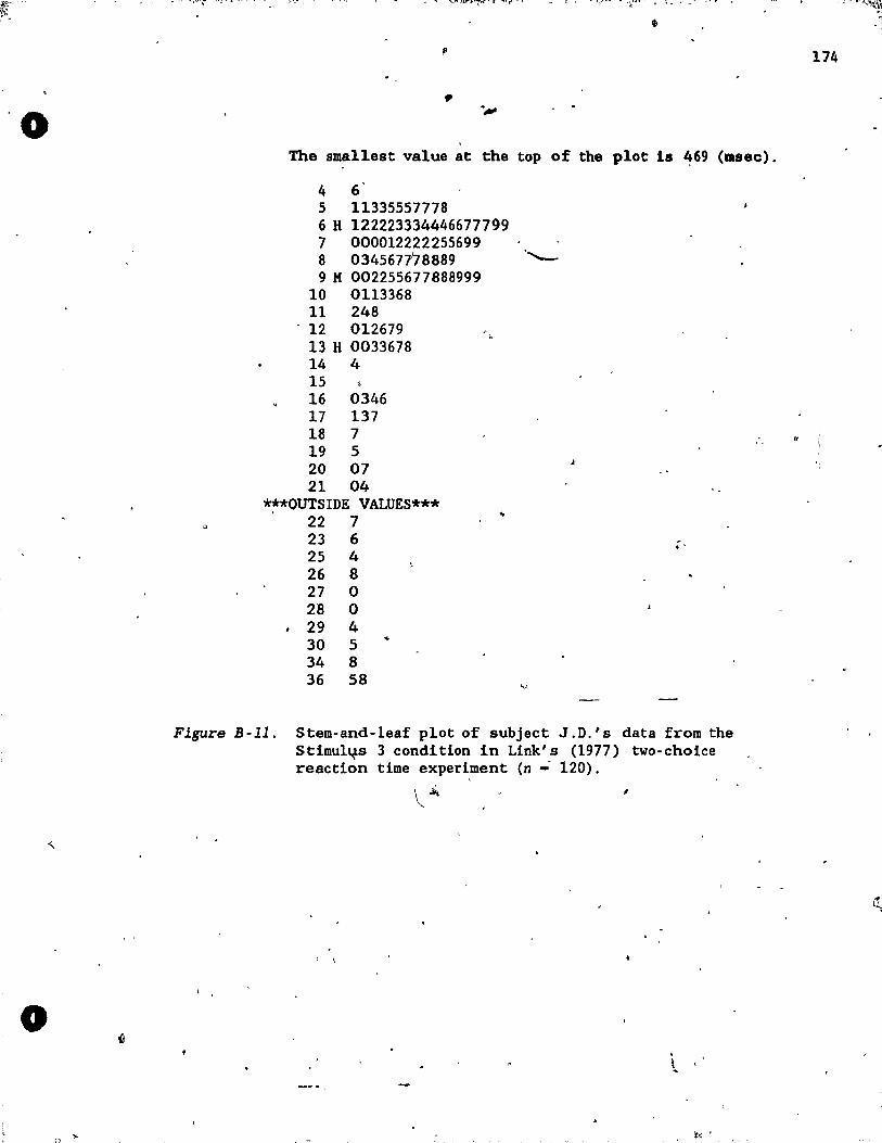
o
o
,.
, The smal1est value at the top of the plot la 469 (lRsec).
4 6 5 11335557778 6 H 122223334446677799 7 000012222255699 8 0345677'78889 9 M 002255677888999
10 0113368 Il 248
- 12 012679 13 H 0033678 14 4 15 16 17 18 19 20 21
0346 137 7 5 07 04
***OUTSIDE VALUES*** 22 7 23 6 25 4 26 8 27 0 28 0 29 4 30 5
.. 34 8 36 58
, •
..
,"
"
Figure B-l!. Stem-and-1eaf plot of subject J.D.'s data from the Stimu1~s 3 condition in Link' s (1977) two-choice reaction Ume expertment (n -- 120).
1
, ,
, "
. t
...
174
1
~ .1
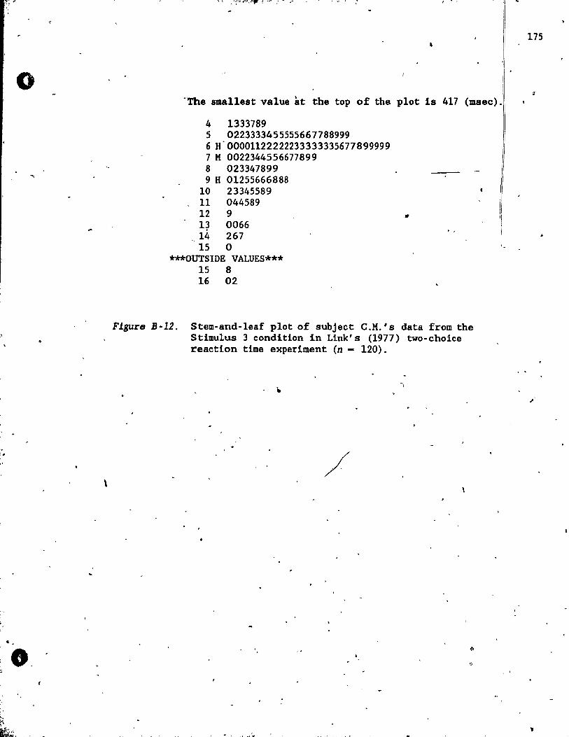
o
'. "
\
o.
.... ,.",--,_.- ," ... __ .. j "."", ""
-The smallest value àt the top of the plot ls 417 (msec).
4 1333789 5 0223333455555667788999 6 U·00001122222233333335677899999 7 M 0022344556677899 8 023347899 9 H 01255666888
10 23345589 11 044589 12 9 1~ 0066 14 267 15 0
***OUTSIDE VALUES*** 15 8 16 02
"
Figure B-12. Stem-and-leaf plot of subject C.M.' s data from the Stimulus 3 condition in Link' s (1977) two-choice react10n Ume exper1ment (n - 120).
/
;t
o
1
175
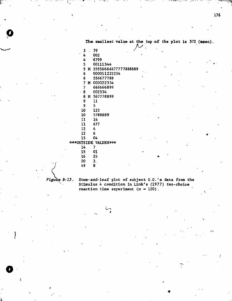
•
o
l , ..... '-:
1'. .. 1 .f'~,"" • .- .... _u ..... ~ .0-1 ~"l"r~J\.'":'<·~ )" .... ~ ... ,I>A.~:·, ~ ~~ ... _.~ •· .... "$~,I· "" .... ~~~.:~\~
~ .. l 'il
-;
176
The smallest value at the top' of the plot Is 372 (lIsac).
3 ' 79 - jJ : '., 4 002 4- '6799 5 00111344 ,. . 5 H 55556666677777888889
'.
6 000011222234 6 556677788 7 M 000022334 7 666666899 8 002334 8 H 567778899 9 11 9 5
10 123 10 5788889 11 14 11 677 12 4 12 6 • 13 04
***OUTSIDE VALUES***
F~ B·B. ,i
. .
14 7 lS 01 16 25 20 3, 49 8
Stem-and-1eaf plot of subject G.G. ' s data from the Stimulus 4 condition in Link's (1977) two-choicè reaction dme experiment (n - 120).
, .
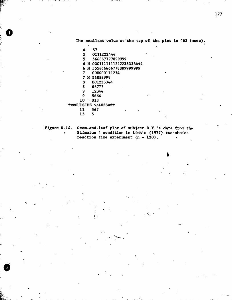
il 't
0 < .-l,:
1"
.-
".
".
The sma11est value atYthe top of the plot is 462 (msec).
4 67 5 0111222444 5 566667777899999 6 H 0001111111222233333444 6 M 555666666778889999999 7 000000111234 7 H 56888999 8 001223344 8 66717 9 12344 9 5666
10 - 013 ***OUTSIDE VALUES***
Il 367 13 5
Figure B-14. Stem-and-1eaf plot of subject B.Y.'s data from the Stimulus 4 condition in Link's (1977) two-choice reaction time experiment (n - 120).
..
"' '
o
177
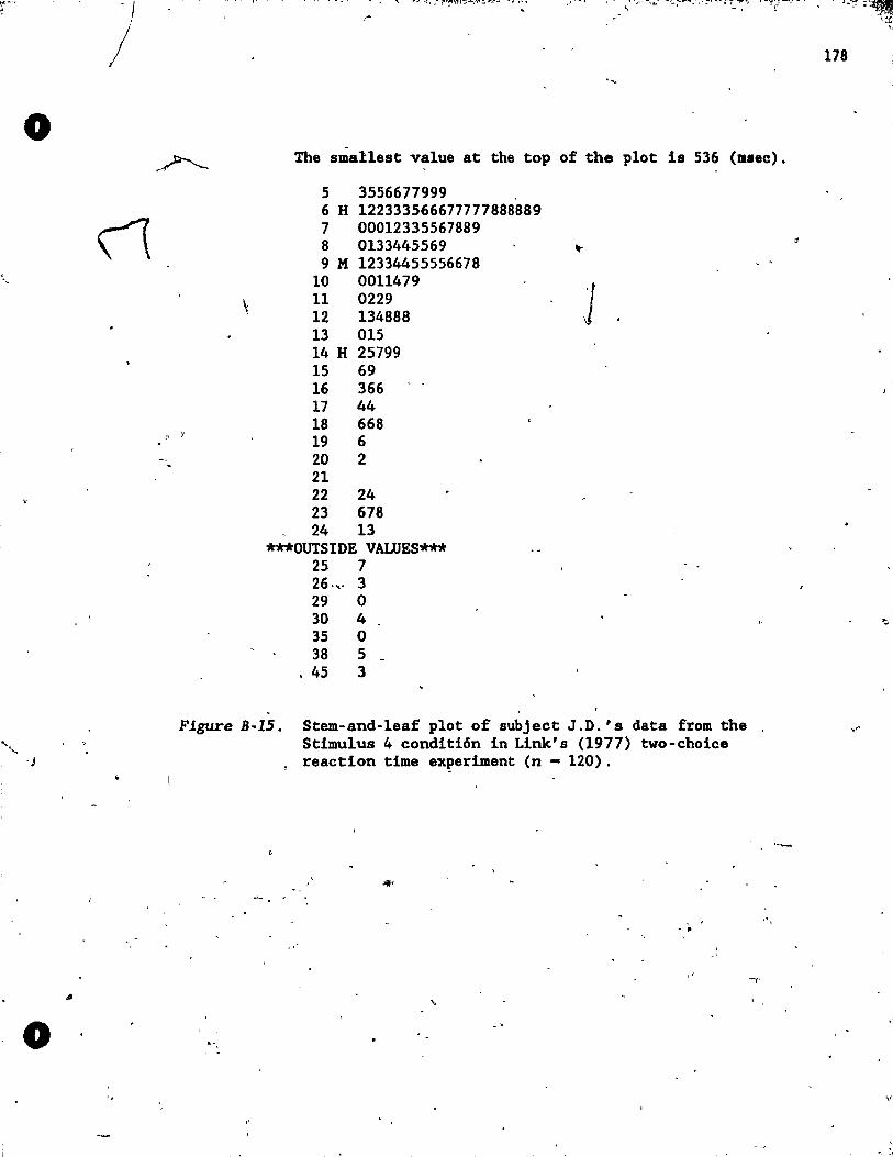
) o
. J
o '.
.. -~.\; ~,." - _.',"; . ~\ '~":.. ~,;;,.. -"_'~~:-;-''!'''''i'''::'~~~~' . j ~1"?'""-t M- .... : •• ~ 1~ ,.:~-;;.
The smal1est value at the top of the plot ls 536 (mile).
5 3556677999 . 6 H 122333566677777888889 7 00012335567889 8 0133445569 9 M 12334455556678
10 0011479 11 0229 12 134888 13 015 14 H 25799 15 69 16 366 17 44 18 668 19 6 20 2 21 22 24 23 678 24 13
***OUTSIDE VALUES*** 25 7 26".· 3 29 0 30 4 35 0 38 5
.45 3
1
Figure B~lS. Stem-and-1eaf plot of subject J.D.'s data from the Stimulus 4 condition in Link's (1977) two-choice reaction time ex~eriment (n - 120) .
-
'.:t
178
v
" ". ~J.
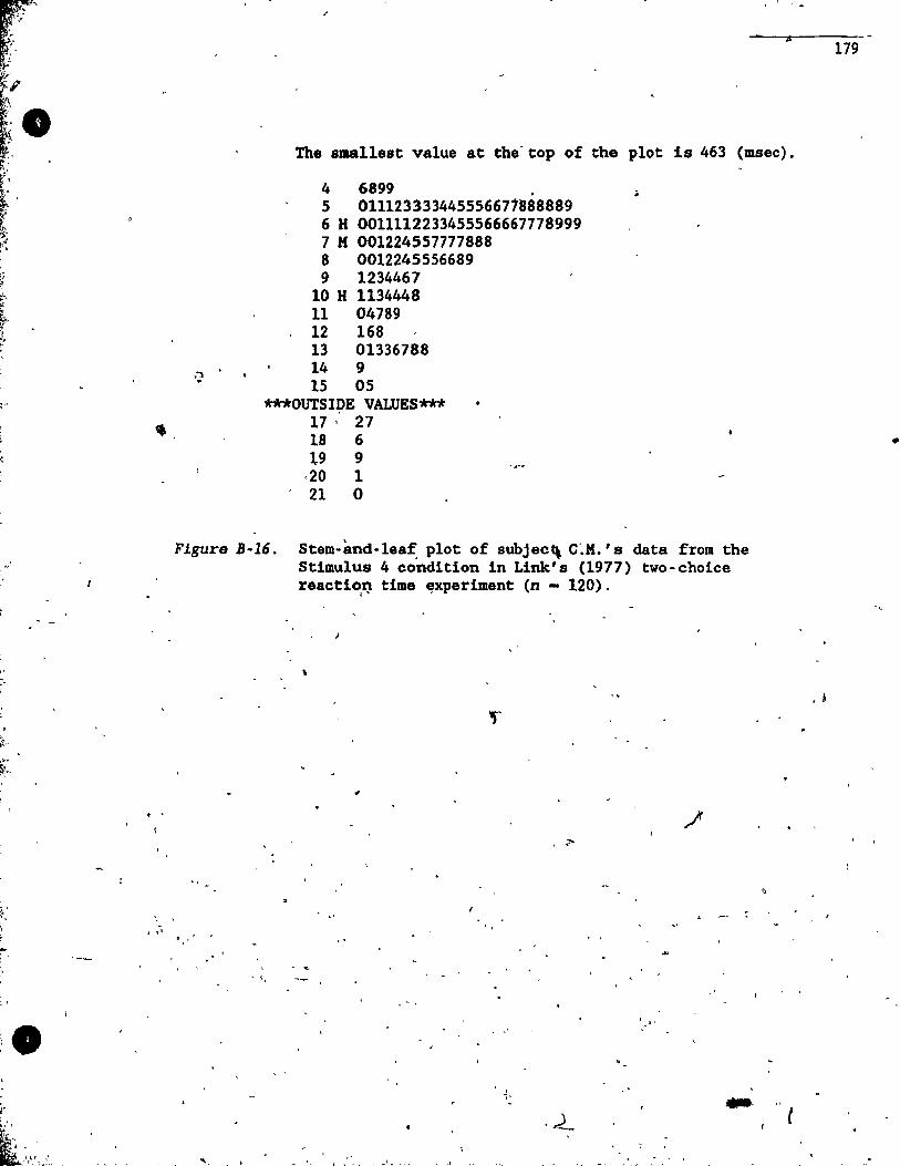
, . .
~,r
~: " "
l'
il
The smallest value at the-top of the plot 1s 463 (msec).
4 6899 • 5 011123333445556671888889 6 H 0011112233455566667778999 7 K 001224557777888 8 0012245556689 9 1234467
10 H 1134448 11 04789 12 168 13 01336788 14 9 15 05
***OUTSIDE VALUES*** 17" 27 18 6 19 9
,20 1 21 0
Figure B-16. Stem-ànd-1eat: plot of subjec\ C'.K.'s data from the Stimulus 4 condition in Link's (1977) two-choice reactl~~ time ~xperiment (n - 120).
\
,..
.' . t,..'
.~-
"
l
179
•
, b
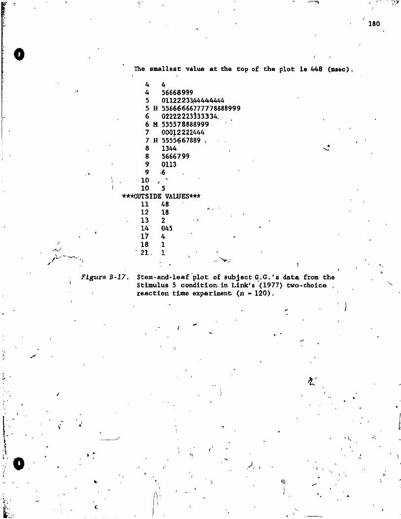
, · :;.
'. · ,
"
-· '
• 1'--
o
-\ . r 'l ; . • 1 • , "
1 • " L
id
K ~? -" ... "......
,-
~.
" ,./!v'
/
\.-'- ___ ~' r , "
1
The sma11est value at the top of the plot la 448 (msee).
4 4 4 56668999 5 01122233,44444444 5 H 55666666777778888999 6 02222223!3333~ 6 M 555578888999 7 00012222444 7 H 5555~67889 _ 8 1344 8 5666799 9 0113 9 ·6
10 10 5
***OUTSIDE VALUES*** 11 48 12 18
0_ '
13 2 . " 14 045
·17 4 18 1
o 21. 1
Figure B-17. Stem-and-leaf plot of subjeet ~.G.' s data from the Stimulus 5 condition. in Link's (1977) two-choiee reaotion time experiment. (n - 120).
rt,.-')
~: ~!
----------, r ~' ...
., ~ ", 1 . .~
" .' ,): ' i
'. "- (!) r
'\
l' <.
•
180
'"
, 1
t -:
. (""
r>
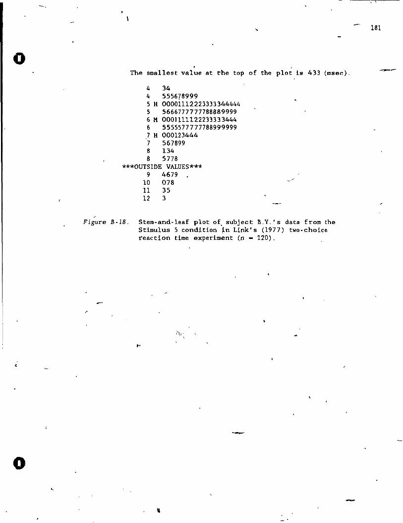
o
o
The smallest value at the top of the plot is 433 (msec).
4 34 4 555678999 5 H 00001112223333344444 5 5666777777788889999 6 M 0001111122233333444 6 5555577777788999999 7 H 000123444 7 567899 8 134 8 5778
***OUTSIDE VALUES*** 9 4679
10 078 11 35 12 3
Figure B-IB. Stem-and-1eaf plot of. subject B.Y.' s data from the Stimulus 5 condition 1.n Link' s (1977) two-choice reaction time experiment (0 - 120).
t,
-
-
· \
181
---
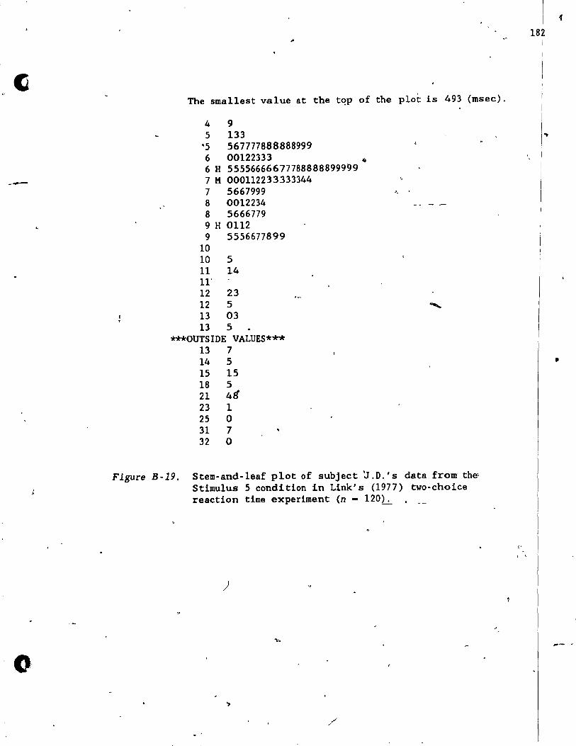
c
-
o
The sma11est value at the t~p of the plot is 493 (msec).
4 9 5 133
"S 567777888888999 6 00122333 41
6 H 55556666677788888899999 7 M 000112233333344 7 5667999 "
8 0012234 8 5666779 9 H 0112 9 5556677899
10 10 5 11 14 11' 12 23 12 5 " 13 03 13 5
***OUTSIDE VALUES*** 13 7 14 5 15 15 18 5 21 4ft 23 1 25 0 31 7 32 0
Figure B-19. Stem-and-leaf plot of subject ~ .D.' s data from the' Stimulus 5 condition in Link' s (1977) two-choice reaction time experiment (n - 120h
)
/
...
•
" -, '
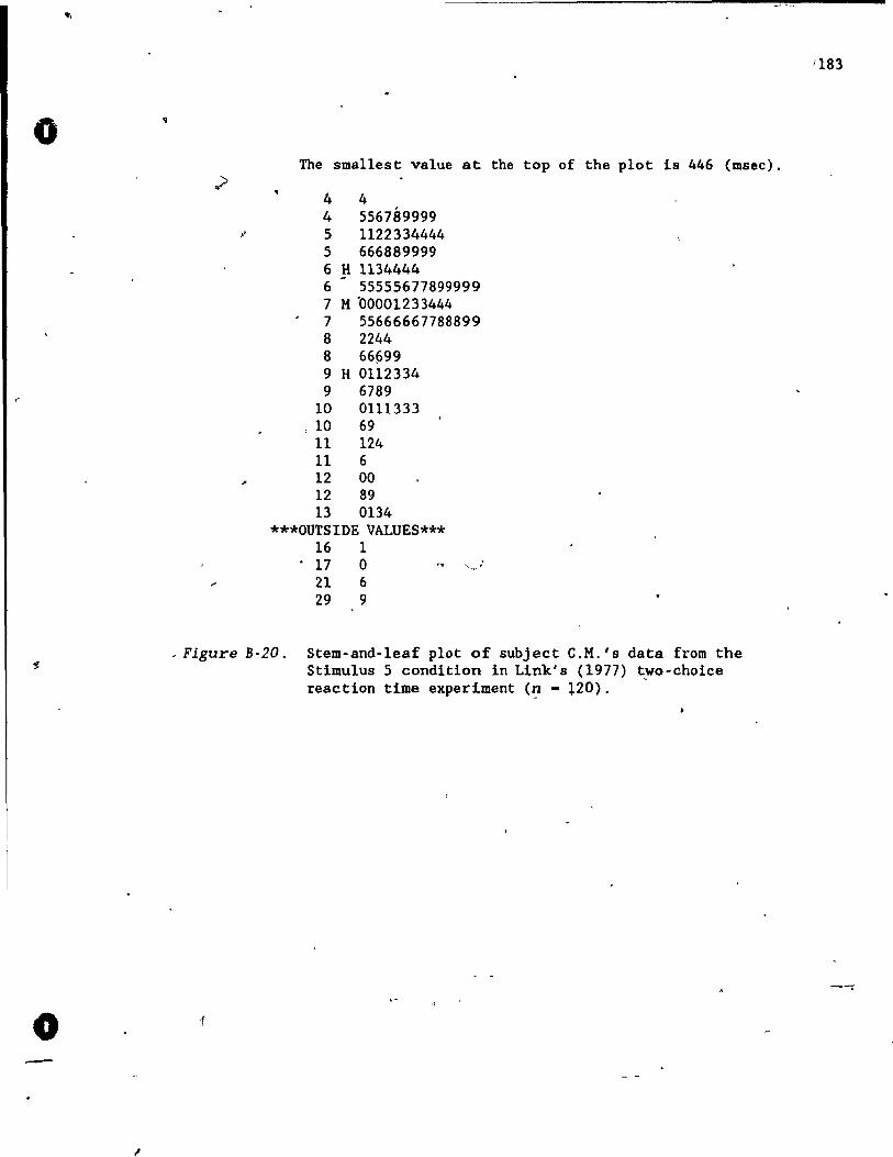
"",
o
r
o -
1
The smallest value at the top of the plot 1s 446 (msec).
4 4 4 556789999 5 1122334444 5 666889999 6 H 1134444 6 55555677899999 7 M '00001233444 7 55666667788899 8 2244 8 66~99 9 H 0112334 9 6789
10 0111333 ,10 69 Il 124 11 6 12 00 12 89 13 0134
***OUTSIDE VALUES*** 16 1
• 17 0 " . 21 6 29 9
• Figure B-20. Stem-and-leaf plot of subject C.M.'s data from the Stimulus 5 condition in Link's (1977) two-choice reaction t1me experiment (~ - l20).
-f
ï183
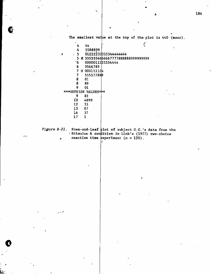
~)
" . ..
•
•
The smallest va e at the top of the p10,t is 440 (msec).
4 44 ( 4 5588899
,5 01222233333344444444 5 M 55555566 6667777888888999999999 ~6 00000112 3334444 6 5566789 7 H 00011112 7 55557788 8 01 8 89 9 01
***OUTSIDE VALUES* *
Figure B-21.
"
9 89 io 4899 12 33 13 07 14 37 17 1
Stem-and-1eaf lot of subject G.G.'s data from the • Stimulus 6 con ition in Link's (1977) two-choice
reaction time xperiment (n - 120). Î
184
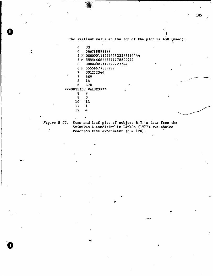
o "" ) The smal1est value at the top of the plot is 430 (msec) .
4 33 4 566788899999 5 H 00000011122222333333334444 5 M 55556666666777778899999 6 00000001112222223344 6 H 55556677889999 7 001222344 7 669 8 14 8 678 '"'
***OUTSIDE VALUES*** 8 9 9_ 0
10 13 11 1 12 4
.r..
Figure B-22. Stem-and-leaf plot ~f subject B.Y.'s data from the Stimulus 6 condition in Link's (1977) two-choice reaction time experiment (n - 120) . t
..
"
185
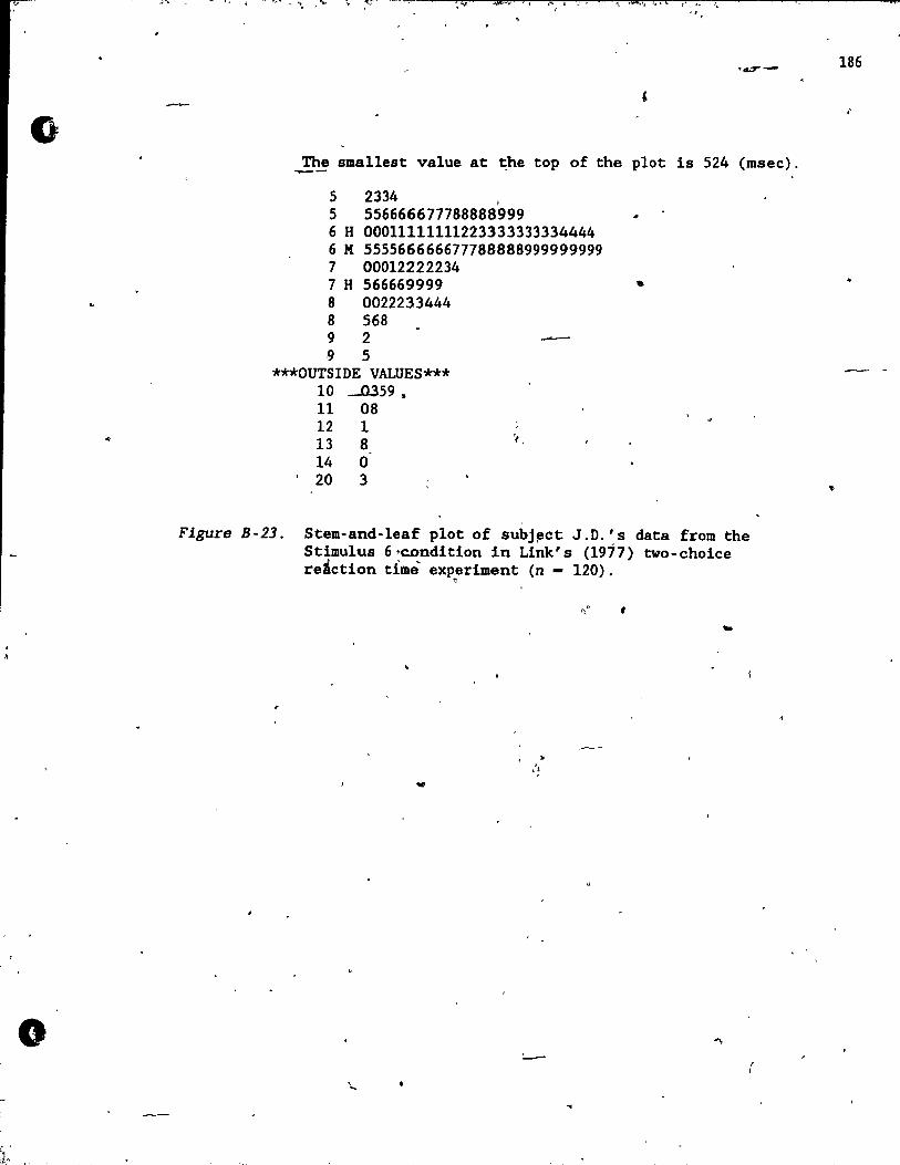
o
,ffi. t 1
", ;Q04Ç.~ ,~ f .. J. 1..-
-,
.~-
The sma11est value at the top of the plot is 524 (msec).
5 2334 , 5 556666677788888999 6 H 00011111111223333333334444 6 M 555566666677788888999999999 7 00012222234 7 H 566669999 8 0022233444 8 568 9 2 9 5
***OUTSIDE VALUES*** 10 -D359. 11 08 12 1 13 8 14 0
'20 3
Figure B-23. Stem-and-1eaf plot of subj~ct J.D.'s data from the Stimulus 6'condition in Link's (1977) two-choice reÂction ti.à experiment (n - 120).
~
1' ... 41 t
r
..
186
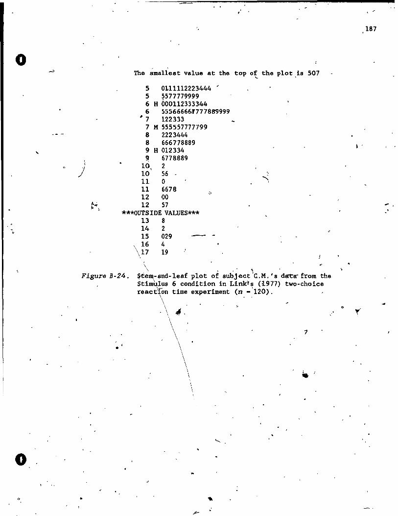
o
o o
)
'.
- ' The smallest value at the top of the plot is 507
'- '
5 Ot11112223444 J
5 ?577779999 6 H 000112333344 6 555666661777889999
~ 7 122333 7 M 555557777799 8 2223444 8 666778889 9 H 012334 ~ 6778889
10~ 2 10 56· Il 0 Il 6678 12 00 12 57
o
***OUTSIDE VALUES***
Figure B-24.
•
•
13 8 14 2 15 029
\ 16 4 \17 19
\ \ . .., .
ste~-and-1eaf plot of subject 'e.M.'s d8:ta- from the Stimulus 6 condition in Link~s (1977) two-choice
\- ' react\on time experiment (n - 120).
\ \ l,
\ 1
\
\ \
\
...
187
"
...

.. <
, >
0
~l 1
~
• ,1
t 1 - .
" r 1
l'If !
~ ..
... 4 •
~\ - .
\:: Q ...
;
'v"
Appendix C .. '. i .,
~ -'1 1
FORTRAN Subroutines •
..
. .
- . ote. Tlle, subroutines ~ete written using FORTRAN 77. > The
International Mà~hematica1 and Statist~cal Library. (IMSL) subroutines GGNPM,-'G9UBS, MDNOR, ZBRENT and ZSPOW, and function ~lN are used in some of the a1gorithms .
. ,~
188
"
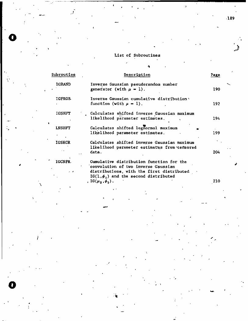
;;
, -- ,<,
,189
....
0 • ,
J List of Subroutines
~
Subroutine DescriEtion Page . , \
!GRAND Inverse Gaussian pseudorandom number '-generator (with ~ - 1). 190
IGPROB. Inverse Gaussian cumulative distribution ~ function (with ~ 1). 192
IGSHFT Calculates shifted inverse Gàussian maximum " likelihood parameter estimates . 194
LNSHFT Ca1cu1ates .. shifted lognormal ~aximum •
lik,elihood parameter estimates. 199
IGSHCR Calculates shifted inv~se Gaussian maximum likelihood parame ter estimat~s from-certsored data. 204
IGCNJ?R. Cumulative distribution function for the il
convolution of two inverse Gaussian distributions, with the first distributed IG(l'~l) and the second distributed
• IG(1'2 '~2) ~ 210 \
, .
o , ,
-
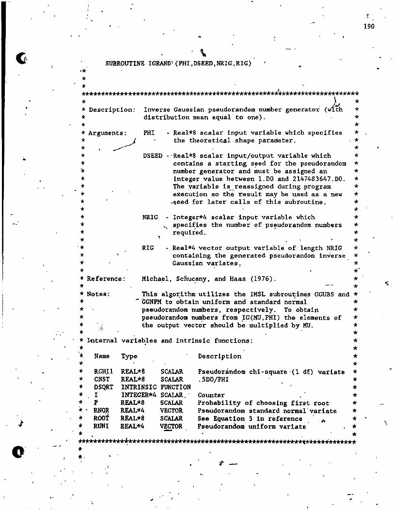
r 1 1
1 . ,
o
\ SUBROUTINE IGRAND~(PHI,DSEED,NRIG,RIG)
.* * * **************************************************,********************* * , * * Description: Inverse Gaussian pseudorand0m number generator (wfth * * distribution mean equa1 to one). * * * * Arguments: PHI - Rea1*8 sca1ar input variable which specifies
the theoretica1 shape parameter. * * * : ,..-/---'
* * ~
* * * * * * * * * ,* * * *
DSEED -'Rea1*8 sca1ar input/output variable which * contains a starting seed for the pseudorandom * number generator and must be assigned an * integer value hetween 1.DO and 2147483647.DO. * The yariab1e is_reassigned during program * execution so the result May be used as a new *
NRIG
?
RIG
-Ejeed for 1ater cal1s of this subroutine. * Integer*4 scalar input variable which
~ specifies the number of ps~udorandom numbers required.
* * * * * - Real*4 vector output variable of length NRIG *
containing the generated pseudorandom inverse * Gaussian variates: *
*' * Referen~e: Micha~l, Scnuc.any, and Haas (1976). *
* * * Notes:
* * * * *
This a1go~ithm utilizes the IMSL subrout1nes GGUBS and * -tGNPM to obtain uniform and standard no~al *
pseudorandom numbers, respective1y. To obtain * pseudorandom numbers from IG(MU,PHI) the e1ements of * the output vector shou1d b~ mu1tiplied by MU. *
* . * Iaterna1 variables and intrinsic functions:
* * * * * * * * * * * * *
'* Name T,ype Description
* * RCH,!l * CNST * DSQRT * 1 * P *. RNOR * Roo! * RUNI
REAL*8 SCALAR REAL*8 SCALAR INTRINSIC FUNCTION INTEGER*4 SCALAR .. REAL*8 SCALAR REAL*4 VECTOR REAL*8 SCALAR REAL*4 VECTOR
Pseudorândom chi-square'(l df) variate .5DO/PHI
Counter Probabi1ity of choosing first root Pseudorandom standard nOrda1'vari~te See Equation 5 in reference b
Pseudorandom uniform variate'
* * ************~****************"""'* '* A A***************,*" U***''It************* * *.
"
~
190
\
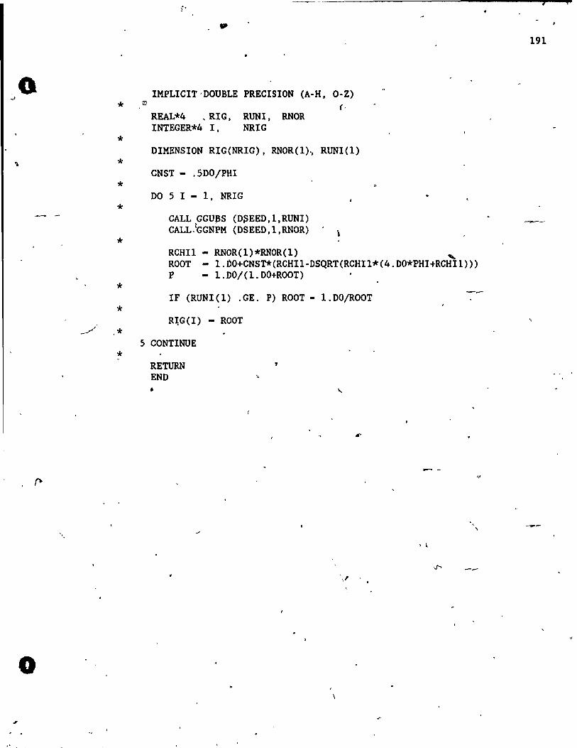
"
o
,
* III
* *
* *
*
* *
.--/ *
i'
•
IMPLICIT'DOUBLE PRECISION (A-H, O-Z) (,
REAL*4 , RIG, RUNI, RNOR INTEGER*4 l, NRIG
DIMENSION RIG(NRIG), RNOR(1)., RUNI(l)
CNST - .5DOjPHI
DO 5 1 - l, NRIG
CALL GGUaS (D~EED,l,RUNI) CALL.~GGNPM (DSEED,l,RNOR) \
RCHIl - RNOR(l)*RNOR(l) "-ROOT - 1.DO+CNST*(RCHI1-nSQRT(RCHI1*(4.DO*PHI+RCHI1») P - 1.DOj(1.DO+ROOT)
IF (RUNI(l) .GE. P) ROOT - 1.DO/ROOT
R~G(I) - ROOT
5 CONTINUE
* RETURN END
"
.,
, l
, El
191
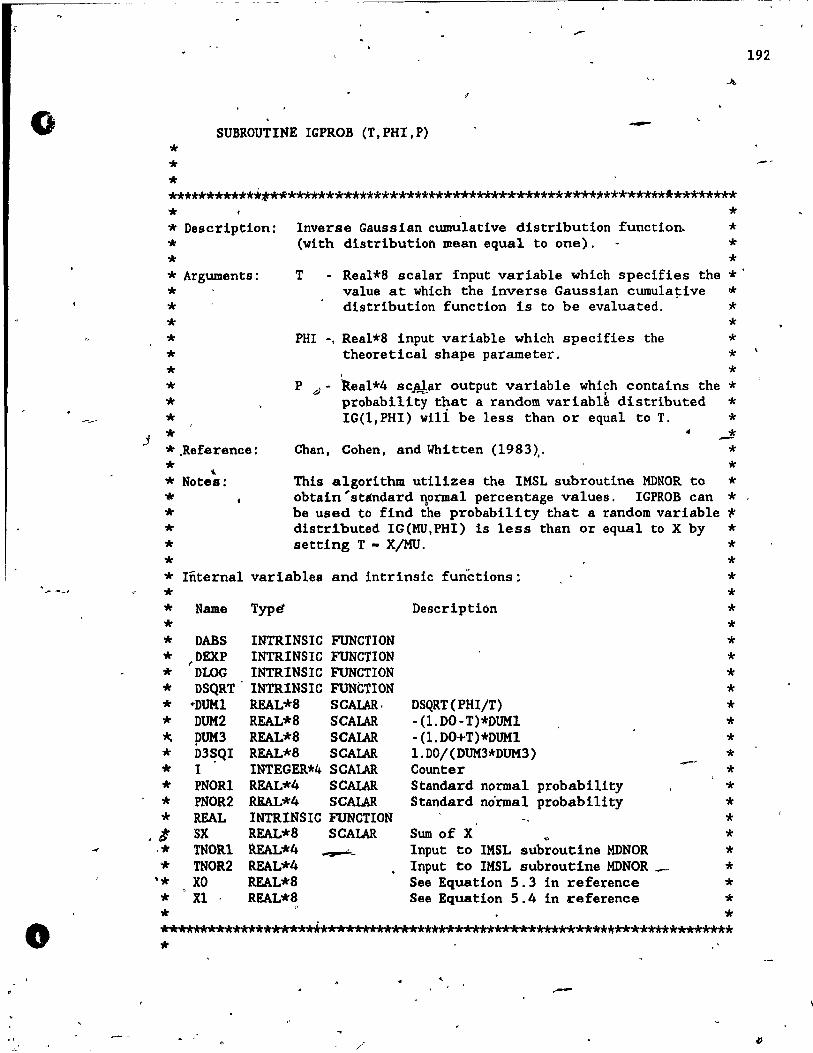
;;
o
o
,>
-SUBROUTINE IGPROB (T, PHI, P)
* * * *************~********************************************************* * * * Description: Inverse Gaussian cumulative distribution function. * * (with distributioi'l Mean equal to one)" *
* * * Arguments: T - Rea1*8 sca1ar input variable which specifies the * . * value at which the inverse Gaussian cumu1a~ive rit
* distribution function is to be eva1uated. '*
PHI -, Rea1*8 input variable which specifies the theoretica1 shape parameter.
* * * *
* * * * * * *
P d - kea1*4 sc.!!ar output variable whi~h contains the * probabillty that a random variabU distributed * IG(l, PHI) wili be 1ess than or equal to T. *
J * * ,Reference:
• Chan, Cohen, and Whitten (1983) .. *
* * .. * Notes:
*' * * *
This algorithm utillzes the IMSL subroutine MDNOR to * obtaln 'stàndard 1'\,ormal percentage values. IGPROB can * be used to flnd the probability that a random variable '/t distributed IG(MU,PHI) 15 less than or equal to X by * setting T - XjMU. *
* * Internal variables and Intrinsic funetions:
* * Name Typè'
* * DABS INTRINSIC FUNCTION * l' DEXP INTRINSIC FUNCTION * DLOG INTRINSIC FONCTION * DSQRT' INTRINSIC FUNCTION * "'DUMI REAL*8 SCALAR· * DUM2 REAL*8 SCALAR '" DUM3 REAL*8 SCALAR . * D3SQI REAL*8 SCALAR * l' INTEGER*4 SCALAR * PNORI REAL*4 SCALAR * PNOR2 REAL*4 SCALAR * REAL INTRINSIC FUNCTION
,1 SX REAL*8 SCALAR ,* TNORI REAL*4 ~_ * TNOR2 REAL*4
'* XO REAL*8 * Xl REAL*8
*
Description
DSQRT(PHljT) - (1. DO-T)*DUMl - (1. DO+T)*DUMI 1. DOl (DUM3*DUM3) Counter Standard normal probability Standard no'rmal probab il It y
Sum of X " Input to IMSL subroutine MDNOR Input to IMSL subroutine MDNOR _ See Equation 5.3 in reference See Equation 5.4 in reference
* * * * * * * * * * * * * * * * * * * * * * *
*******************À****************************************************
*
---/
192
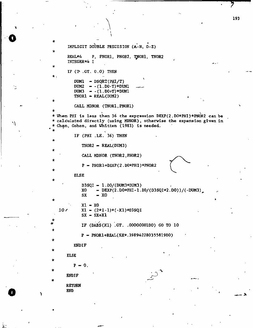
" -"0
~~
"'"
,.,.
0
. :\;,7
*
*
*
*1
*
*
\
.\ 1 \
, . IMPLICIT DOUBLE PRECISION (A-H, O-Z)
REAL*4 P, PNOR1, PNOR2, ~OR1, TNOR2 INTEG'ER*4 l
IF (1l' .GT. O.~) THEN
DUMl - DSQRT(P~I/T) DUM2 - -(l.DO-T)*DUMl DUM3 - -(l.DO+T)*DUMl TNOR1 - REAL(DuH2)
CALL MONOR ('TNORl,PNOR1) . , * When PHI i9 less than 36 the expression DEXP(2.DO*PHI)*PNOR2 can be * calculated directly (using MONOR) , otherwise the expansion given in * Chan, Cohen, and Whitten (1983) 18 needed.. . . * *
* * * *
*
* il!'
* * * *
*
*
•
IF (PHI .LE. 36) THEN
TNOR2 - REA'L(DUM3)
CALL MONOR (TNOR2,PNOR2)
P - PNOR1+DEXP(2.DO*PHI)*PNOR2
ELSE
D3SQI - 1.DO/(DUM3*DUM3) XO - DEXP(2.DO*PHI-l.DO/(D3SQI*2.DO»/(-DUM3) SX - XO
Xl - XO 10 l' Xl - (2*1 -1)*( -Xl)*D3SQI
SX - SX+Xl . / ,
IF (DABS(Xl) .GT .. OOOOOOOlDO) GO TO 10
P - PNORI+REAL(SX*.398942280355819DO)
ENDIF
ELSE
P - O.
ENDIF ~~ --'
RETURN END
-
,.
193
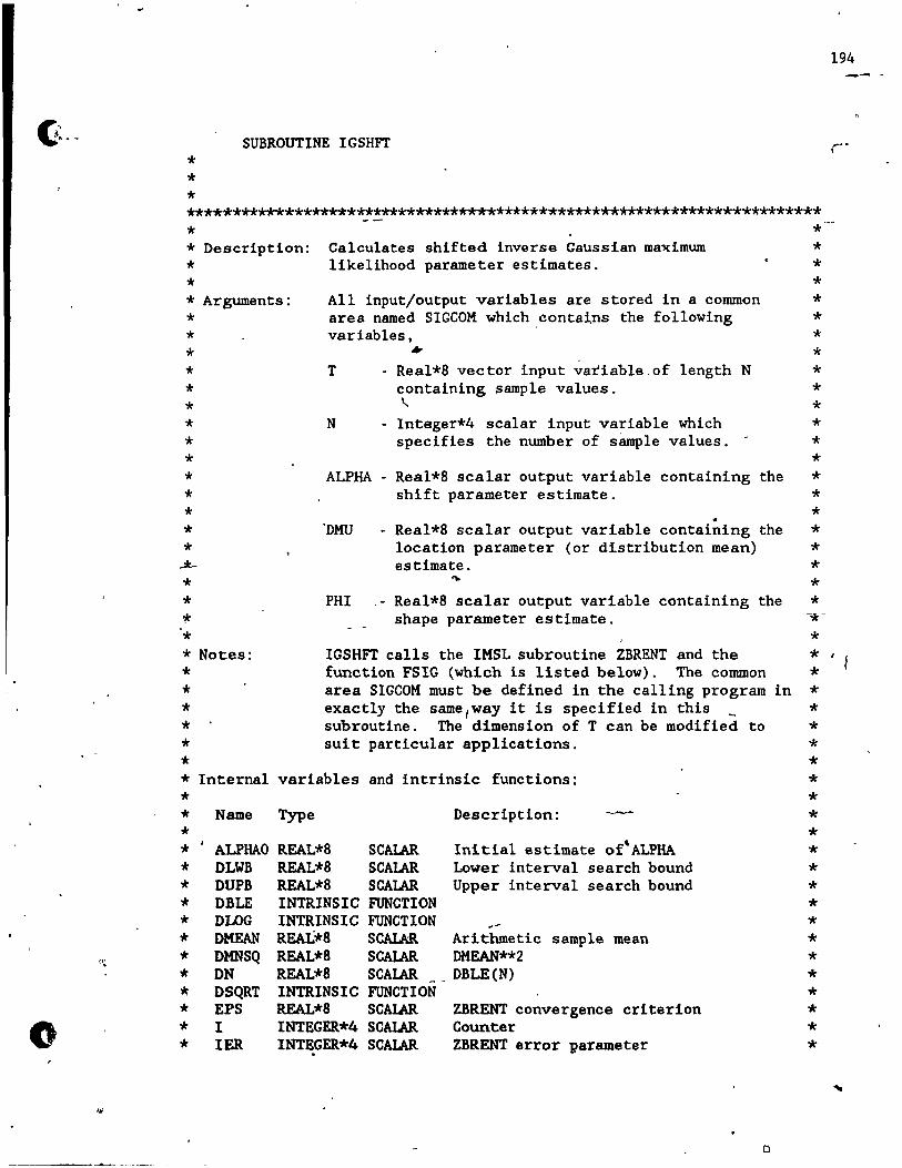
~:_-
o
SUBROUTINE IGSHFT
* * * ************************************************************************
* * * Description:
* * * Arguments:
* * * * * * * * * * * * * *
-*-
* * * *
Calculates shifted inverse Gaussian maximum likelihood parameter estimates.
AlI input/output variables are stored in a common area named SIGCOM which contains the following variables, .., T - Real*8 vec tor input variable- of length N
N
containing sample values. \..
- Integer*4 scalar input variable ltthich specifies the number of sample values. -
ALPHA - Real*8 scalar output variable containing the shift parame ter estimate.
-"DMU - Real*8 scalar output variable containing the location parameter (or distribution mean) estimate.
'" PHI - Real*8 scalar output variable containing the
shape parame ter estimate.
* * * * * * * * * * * * * * * * * * * * * -*
*
194
* Notes:
* IGSHFT caUs the IMSL subroutine ZBRENT and the function FSrG (which i8 listed below). The common area SIGCOM must be defined in the calling pro gram in exactly the same/way it is specified in this _ subroutine. The dimension of T can be modified to suit particu1ar applications.
* 1 i *
* * * * * * * * * * * Interna1 variables and intrinsic functions: * * * * Name Type Description: * * * * ALPHAO REAL*8 SCMAR Initial estimate of' ALPHA * * DLWB REAL*8 SCMAR Lower interva1 search bound * * DUPB REAL*8 SCAIAR Upper interval search bound * * DBLE INTRINSIC FUNCTION * * DLOG INTRINSIC FUNCTION ~_ * * DMEAN REAL*8 SCALkR Arithmetic samp1e mean * * DMNSQ REAL*8 SCAIAR DMEAN**2 * * DN REAL*8 SCMAR __ DBLE(N) * * DSQRT INTRINSIC FUNCTION * * EPS REAL*8 SCAIAR ZBRENT convergence criterion * * 1 INTEGER*4 SCAIAR Counter * * 1ER INTEGER*4 SCAIAR ZBRENT error Rarameter *
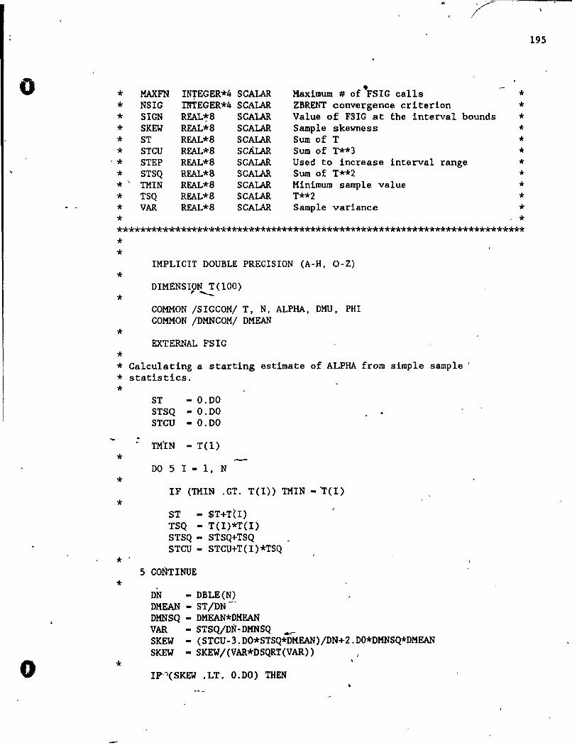
0
o
• * MAXFN INTEGER*4 SCALAR Maximum # of FSIG ca1ls * * NSIG mTEGER*4 SCALAR ZBRENT convergence criterion * * SIGN REAL~8 SCALAR Value of FSIG at the interval bounds * * SKEW REAL*8 SCALAR Sample skewness * * ST REAL*8 SCALAR Sum of T * * STCU REAL*8 SCÀLAR Sum of T**3 *
,* STEP REAL*8 SCALAR Used to increase interva1 range * * STSQ REAL*8 SCALAR Sum of T**2 * * '. TMIN REAL*8 SCALAR Minimum samp1e value * * TSQ REAL*8 SCALAR T**2 * * VAR REAL*8 SCALAR Sample variance * * - * ************************************************************************ * * * *
*
*
IMPLICIT DOUBLE PRECISION (A-H, O-Z)
DIMENSION T(IOO) "--COMMON ISIGCOMI T, N, ALPHA, DHU, PHI COMMON 10MNCOMI OMEAN
EXTERNAL FSIG
* Calculating a starting estimate of ALPHA from simple samp1e ' * statistics.
*
* *
*
* *
*
ST - 0.00 STSQ - 0.00 STCU - 0.00
TMIN - T(l)
OOSI-l,N
IF (THIN .GT. T(I» TMIN -'T(l)
ST - ST+T~I) TSQ - T(I)*T(I) STSQ - STSQ+TSQ STCU - STCU+T(I)*TSQ
5 CONTINUE
DN - DBLE(N) OMEAN - ST/DN-DMNSQ - DMEAN*DMEAN VAR - STSQ/DN-DMNSQ __ SKEW - (STCU-3.00*STSQ*DMEAN)/DN+2.DO*DMNSQ*DMEAN SlŒW - SKEW/(VAR*DSQRT(VAR»
Ip'1(SKEW . LT. O.DO) THEN
195

,
..
* WRITE(*.'(A)') , ERROR: The sample skewness is negative.'
* GO TO 9999
* ENDIF
* ALPHAO - TMIN-«DMEAN-TMIN)**3)/(2.DO*VAR*DLOG(DN» , * * Looking for reasonable upper and lower bounds for the search * interval.
*
* *
*
* * *
*
* * *,
*
* *
* * *
*
10
SIGN - FSIG(ALPHAO)
IF (SIGN .GE. O.DO) THEN
STEP - .1DO*(TMIN-ALPHAO) DUPB '- ALPHAO \ DLWB - DUPB DUPB - DLYB+STEP
IF (DUpa .GE. TMIN) THEN ,
WRITE(*,'(A)') , ERROR: No valid search interval found.'
GO TO 9999
ENDIF
SIGN - FSIG(DUPB)
IF (SIGN .GE. O.DO) GO TO 10
ELSE
STEP - .1DO*ALPHAO DLWB - ALPHAO
1 •
15 DUPB - DLYB DLWB - DUPB-STEP
IF (DLYB .LT. O.DO) THEN
WRITE(*.' (A):) , ERROR: No vaUd searcn interval found.'
GO TO 9999
ENDIF
SIGN - FSIG(DLYB)
IF (SIGN .LE. O.DO) GO TO 15
r
19
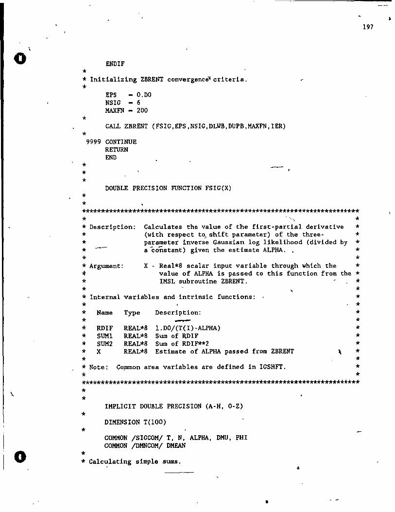
, o
\
o
ENDIF
* * Initializing ZBRENT convergence~criteria.
* EPS 0.00 NSIG 6 MAXFN 200
* CALL ZBRENT (FSIG,EPS,NSIG,DLWB,DUPB,MAXFN,IER)
* 9999 CONTINUE
RETURN END
* * *
DOUBLE PRECISION FUNCTION FSIG(X)
* * ************************************************************************ * ", * * Description: Calculates the value of the first-partial derivative * * (with respect to" shift parameter) of the three- * * parame ter inverse Gaussian log likelihood (divided by * * a -constant) given the estimate ALPHA. • *
* * * Argument:
* * *
x - Real*8 scalar input variable through which the value of ALPHA is passed to this function from IMSL subroutine ZBRENT.
* InternaI variables and intrinsic functions:
* * Name *
* RDIF * SUMI * SUM2 * X * * Note: *
Type Description:
REAL*8 REAL*8 REAL*8 REAL*8
-1.DO/(T(I)-ALPHA) Sum of lU)IF Sum of RDIF**2 Estimate of ALPHA passed from ZBRENT
C~~on are a variables are defined in IGSHFT.
* the *
* * * * * * * * *
\ * * * *
************************************************************************
* * *
*
*
IMPLICIT DOUBLE PRECISION (A-H, O-Z)
DIMENSION T(lOO)
COHMON /SIGCOM/ T, Nt ALPHA, DHU, PHI COHMON /DMNCOM/ DMEAN
* Calculating simple sums.
•
197
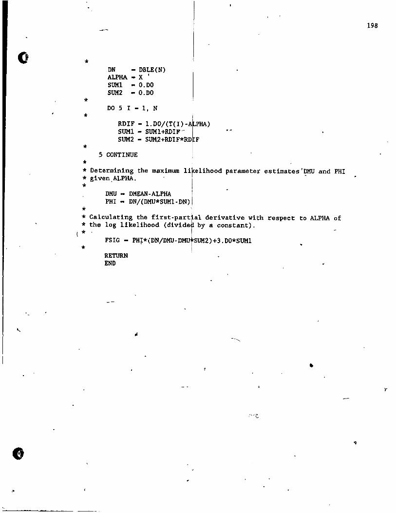
Cl *
*
*
*
*
DN - DBLE(N) ALPHA - X 1
SUMl - O.DO SUM2 - O.DO
DOSI-l,N
RDlF - 1.DO/(T(I)-A PRA) SOM1 - SUMl+RDIF-SOM2 - SUM2+RDIF*RD F
5 CONTINUE
* Determining the maximum li e1ihood parame ter estimates'~MU and PHI * given,ALPHA.
e
* DHU - DMEAN-ALPRA 1
PHI - DN/(DHU*SUM1-DN),
* * Calculating the first-pardal derivative with * the log likelihood (divideh by a constant).
l * ' r * FSIG - PH~*(DN/DHU-DMUtSUM2)+3.DO*SUM1
RETURN END
1
----~~-- -~-.
respect to ALPHA of
..
•
198
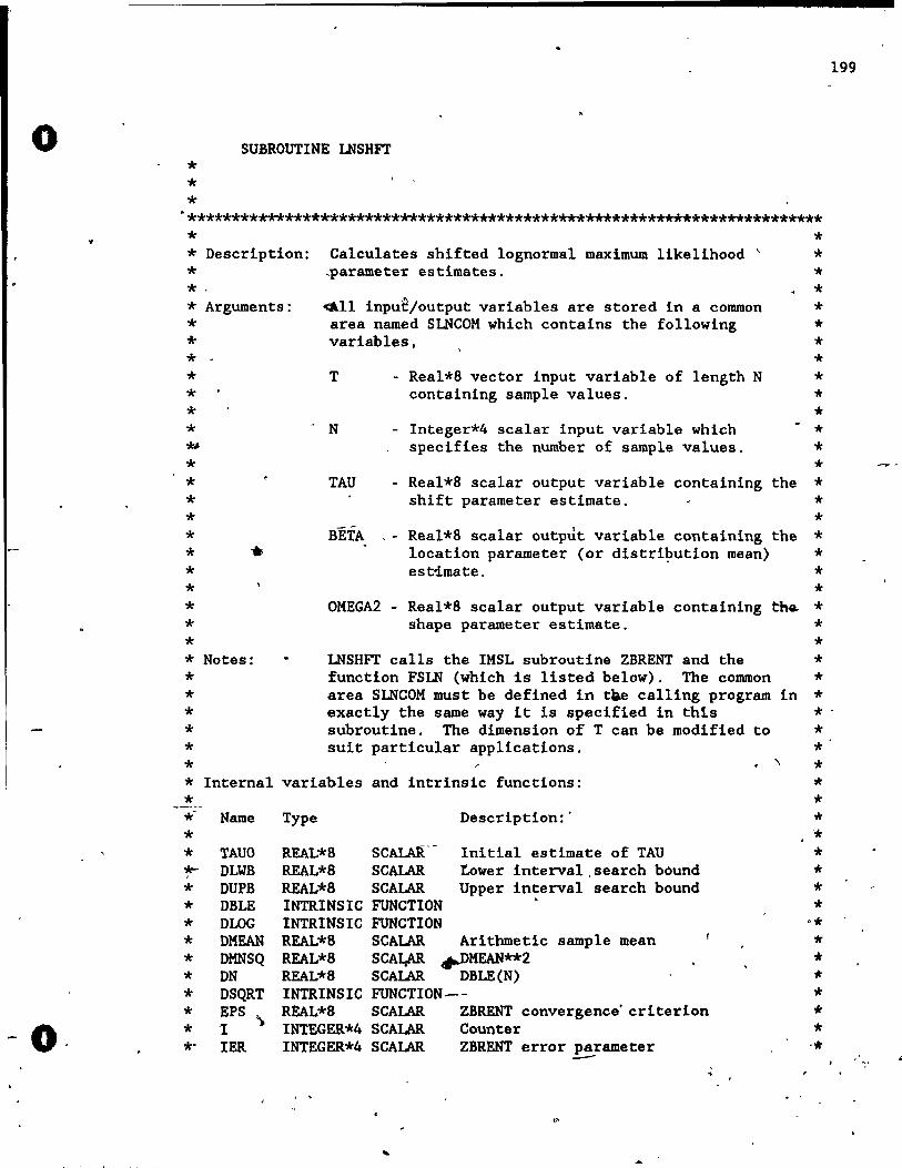
o
O·
* * *
SUBROUTINE LNSHFT
199
"************************************************************************ * * Description: Ca1cu1ates shifted lognormal maximum likelihood '
_parameter estimates. * *, * Arguments:
* ~ll inpuê/output variables are stored in a common area named SLNCOM which contains the fol1owing variables, * * .
* * * * -* * * * * * * * * * * * Notes:
* * * * * *
T
, N
TAU
B"ETA
- Real*8 vector input variable of length N containlng sample values.
- Integer*4 scalar input variable which specifies the number of sample values.
Real*8 scalar output variable containing the shift parameter estimate.
- Real*8 scalar output variable containing the location parameter (or distri~ution mean) estimate.
OMEGA2 - Real*8 scalar output variable containing th~ shape parameter estimate.
LNSHFT calls the IMSL subroutine ZBRENT and the function FSLN (which ls listed below). The common area SLNCOM must be defined in tae calling pro gram in exactly the same way it is specified in thts subroutine. The dimension of T can be modified to suit particular applications. . \
* InternaI variables and intrinsic functions: *
----~
'* Name * * TAUO ok- DLlI)'B * DUPB * DBLE * DLOG * DMEAN * DMNSQ * DN * DSQRT * EPS \ * "I *. 1ER
Type
REAL*8 SCALAR:'-REAL*8 SCALAR REAL*8 SCALAR INTRINSIC FUNCTION INTRINSIC FUNCTION
Description: .
Initial estimate of TAU tower interval,search bound Upper interval search bound
REAL*8 SCALAR Arithmetic sample mean REAL*8 SCAI,AR .,nMEAN**2 REAL*8 SCALAR DBLE(N) INTRINSIC FUNCTION---REAL*8 SCALAR ZBRENT convergence' criterion INTEGER*4 SCALAR Counter INTEGER*4 SCALAR ZBRENT error parame ter
.;;.--. .
* * * * * * * * * * * * * * *
* *
* *
* * * *
* * * * *. * * * * * * '* * * * *
0*
* * * * * * ,*
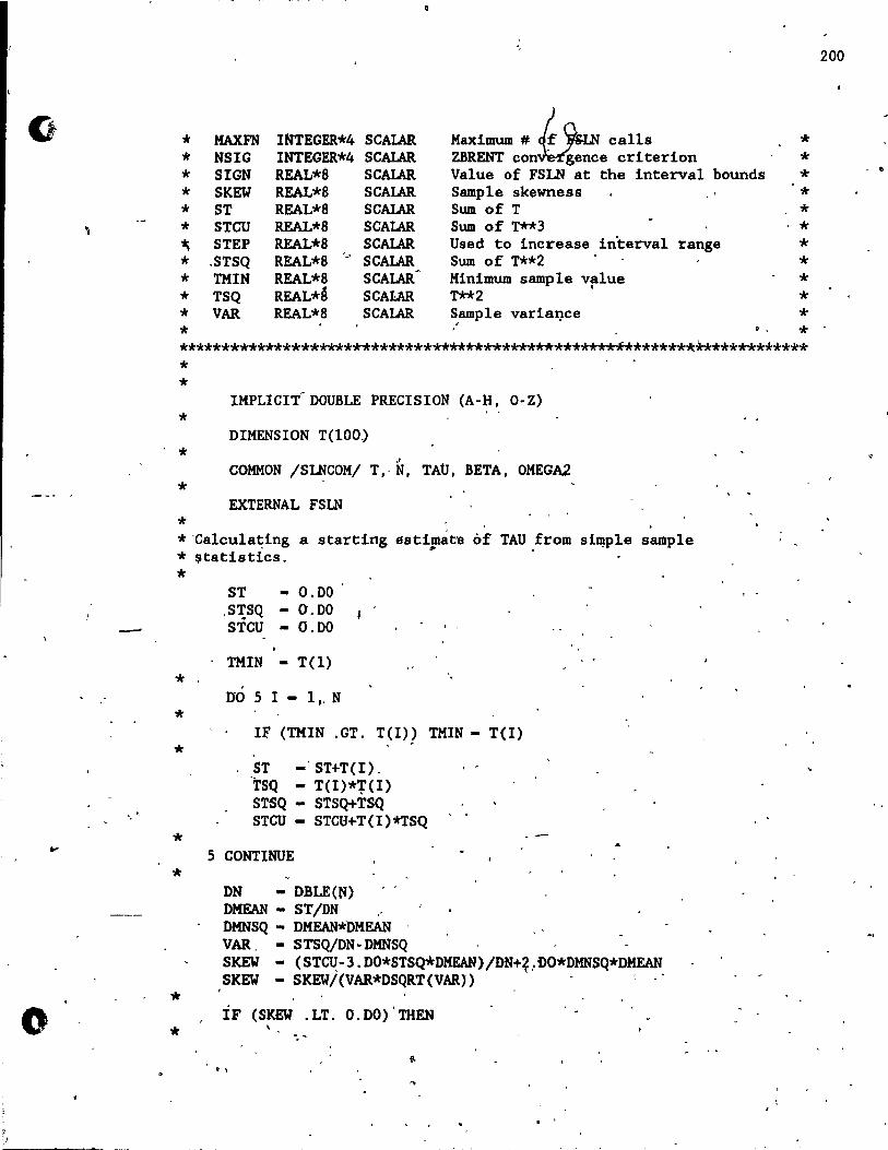
(}
'\
~. "
o
,
* KAXFN INTEGER*4 SCAlAR lIaxiaum # ~ calls * * NSIG INTEGER*4 SCAlAR ZBRENT con - gence criterion * * SIGN REAL*8 SCAlAR Value of FSLN at the interval bounds * * SKEW REAL*8 SCAlAR Sample skewness * * ST REAL*8 SCAlAR Sum of T * * STCU REAL*8 SCAlAR Sum of T**3 .* ~ STEP REAL*8 SCAlAR Used to increase in'terval range * * .STSQ REAL*8 '-, SCAlAR Sum of T**2 * * THIN REAL*8 SCAlAR
0
Minimum sample v~lue * * TSQ REAL*A SCAI:.AR T**2 * * VAR REAL*8 SCAlAR ~ample varia~ce * * o • * **************************************************~********************* * *
IMPLICIT- DOUBLE PRECISION (A-H, O-Z) *
DIMENSION T(lOO) *
~
TAU, COMMON /SLNCOM/ T,-N, BETA, OMEGA2 *
EXTERNAL FSLN
* * 'Calcula~ing a starting esti~aée of TAU from * $tatistics. .
si~ple sample
*
* * *
* *
* *
ST ,S~SQ STCU
O.DO O.DO a.DO
THIN - T(l) ,
DO 5 I - l,. N
IF (THIN .GT. T(I» TMIN - T(I)
ST -' ST+T(I). "TSQ - T(I)*'r(I) STSQ - STSQ+TSQ STeu - STCU+T(I)*TSQ
5 CONTINUE
DN - DBLE(N) DHEAN - ST/DN .' DHNSQ - DHEAN*DHEAN VAR. - STSQ/DN~DMN'SQ SKEY - (ST~ ~ 3 . DO*STSQ*DMEAN) /DN+~ " i>O*DMNSQ*DMEAN
,SKEY - SKEY/(VAR*DSQRT(VAR) .
iF (SKEW .LT. O.DO)'THEN
. ,
200
•
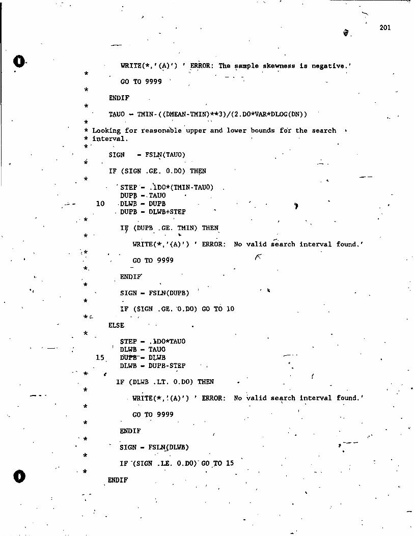
...;. -
..
o
f.
WRITE(*,'(A)') , ERROR: The ~ampl& skewness is negative.'
* " GO Ta 9999
* ENDIF
* ~~UO - TMIN-«DMEAN-TMIN)**3)/(2.DO*VAR*DLOG(DN»
* * Looking for reasonàble upper and lower bounds fo'r the search * interval. *'
*
.*
SIGN - FS~(TAUO)
IF (SIGN .GE. O.DO) TH~N
'STEP'- .1DO*(TMIN-TAUO) OUP\\ -,TAUO
10 ,DLWB - DUPB . DUPB - DLWB+STEP
IV (DUPB, .GE. TMIN) THEN * ~
* * *
*
- *.
* * *
,*
* *
WRITE(*,'{A)') , ERROR: No valid ~arch interval found.'
GO TO 99g9
ENDIF"
SIGN - FSLN(DUPB)
IF (SIGN .GE. ·O.DO) GO TO 10
ELSE
STEP - . }OO*TAUO DL~ - TAUQ
15 DtJn-- D~WB DLWB - DUPB-STEP
t IF (DLWB .LT. O.DO) THEN
. WRITE(*,~(A)') , ERROR:
GO Ta 9999
ENDIF
SIGN - FSLNJDLWB)
IF-(SIGN .LE. 0.DO)-GO.10 15
ENDIF
, \
(
No valid searcn interval found.' ,
,
\
201
.'
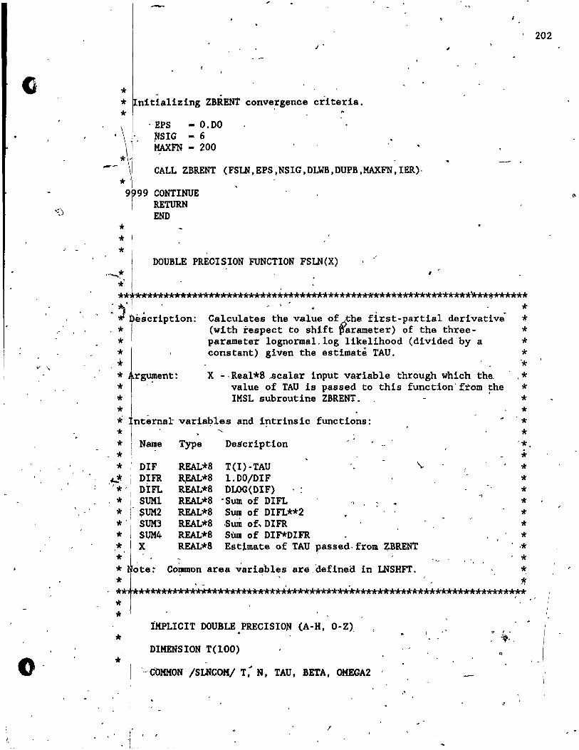
to' \,
o
* * *
J •
" . nitializing ZBRENt conve;gence criteria.
. EPS - O.DO ~SIG - 6 MAXFN - 200 " .):"
-- *\ CALL ZBRENT (FSLN,EPS,NSIG,DLWB,DUPB,MAXFN,IER)· *'
9p99 CONTINUE 1 RETURN
END
* * 1
* , , ......... * 1 DOUBLE PREOIS.ION FUNC~ION FSLN(X) .' , 0 •
" ~t**···**********~~·~**~··*****************·*****~********: "~ièSèriPtl0n: Calculates the value of9~he flrst-partlal derivative * . * (with respect to shift parameter) of the three- *
* parame ter lognormal.log likellhood (divlded by a * * constant) glven the estlmate TAU. * ,~ ~
* rg~ent: X --Real*8 .scalar input variable through which th~ * * value of TAU Is passed to this functlon'ftom the * * IMSL subroutine ZBRENT. ' *
* * ntèrnarvaria~les and intrinsic functions:
* * *' * * *
Name
DIF DIFR DiFL SUln SUM2 SUM3 SUM4 X
Type
REAL*8 ~EAL*8 REAL*8 REAL*8 REAL*~ REAL*8 REAL*8 REAL*8
'DeScription
T(I)':TAU l.DO/DIF DLOG(DIF)
'Som of DIFL Som of DIFL**2 Sum of .. DIFR Sùm of DIF*DIFR Estlmate of TAU ~assed·from
\.
~BREN'l'
* * *
* * * * * * * * .* * "> 'J~ \ -,
* Common are a varIables are.defined in LNSHFT. * * "Ir
r ** *********************************************************************
* * * *
iMPLICIT DOUBLE ,PRECISION (A-H, O-Z).
DIMENSION T(lOO)
'-COKKON /SLNCOM/ T," N, TAU, BETA, OKEGA2 '
,
'" ,. """ ., ...
"
202
.. i.
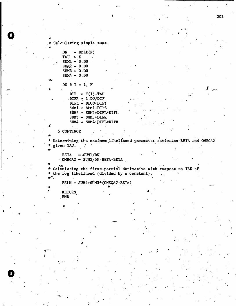
o "
-
1
o
..
* .* Calculating slmple,sums.
*
*.
*
-'
*
DN • DBLE(N) TAU • X SOMI ·'O.DO SOM2 - O.DO StJM3 .. 'O. DO SOM4,- O.DO
D05I-l,N
DIF - T(I) -TAU .DIFR ~ 1.DO/DIF DIFL - DLOG(DIF) SUMl - SUMl+DIFL SOM2 - SUM2+DIFL*DIFL SUM3 - SUM3+DIFR SUM4 - SUM4+PIFL*DIFR
5 CONTINUE
"
, ,
* ' ,
1
. , - - Il ' -* Determining the maximum,llkelihood parameter estimates'BETA an4 OMEGA2 ~ gi ven TAU. .-' - - , ',. * ' '
BETA -.SUMl/DN . OMEGA2 - SUM2/DN -BETA*BETA
'* ..... - ~ * Calculating the first-partiâl derivative with respect to TAU of * the log Ukelihood (divided by a constant'). *-',' .
FSLN - SUM4+SÙM3*(OMEGA2-BETA) * • y RETURN
,END
, ,
1 l'
\
• ,t ..
"
.'
•
, \
...
" ,
, ' " , , .
"
203.
-..
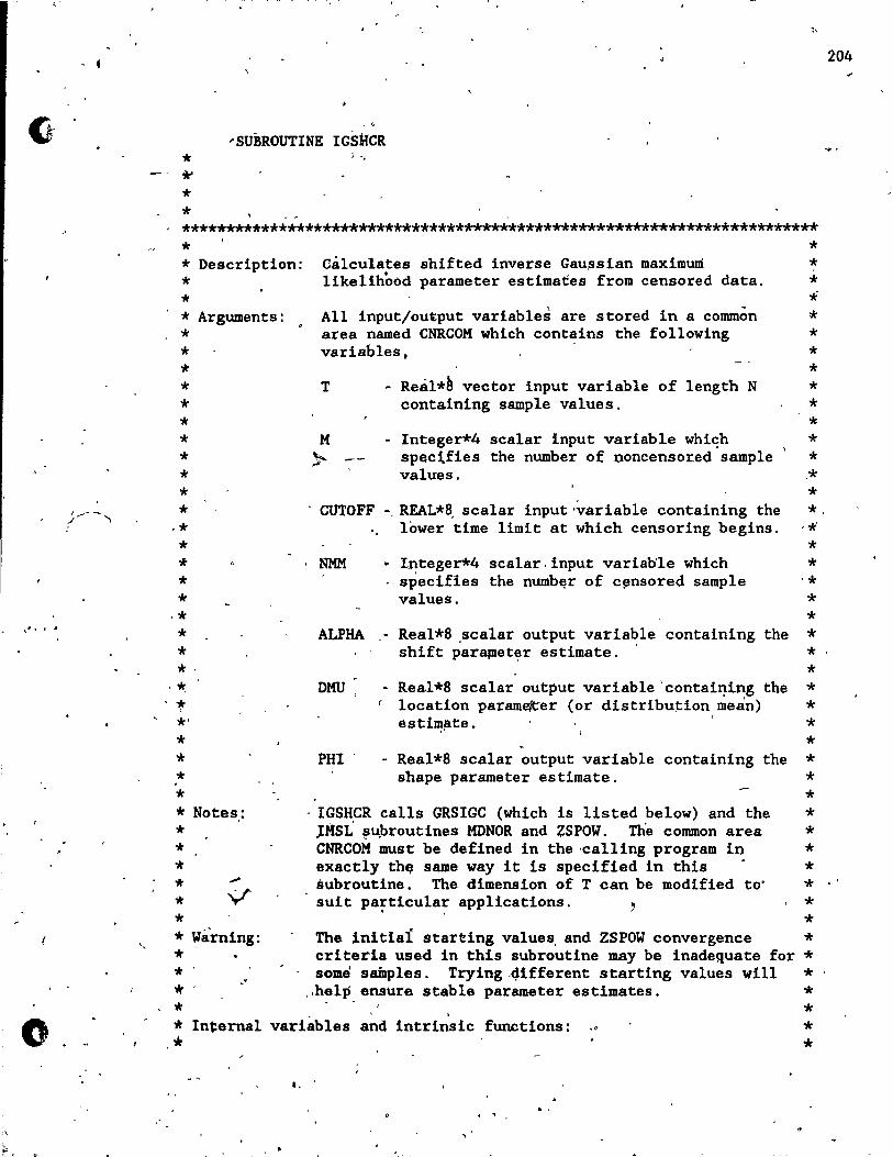
;/-"
"
o
:,. : ' ,li
, , 'SUBROUTINE IGSHCR
* *' * *
Î ",.
************************************************************************ * * Calculates shifted inverse Gau~sian maximum *
likelihood parame ter estimates from censored data. * * Description: * * * Arguments: * * * * * * * * * * *
-* * 'Ii:
* *
.* * * *,
.*.
~ *, * * * . * * Notes,: * * * * ,.,;
* V *
* Ws.rning:
* * . *
. *,
AlI input/output variables are stored in a common * area named CNRCOM which contains the following * variables. *
T - Real*~ vector input variable of length N containing sample values.
- Integer*4 scalar input variable which spec~fies the number of noncensored sample values.
* * * * * * .* * CUTOFF ., REAL*8, scalar input ';'ariable containing the * ,
lower time limit at which censoring begins. ,*'
NMM ~ Integer*4 scalar, input variab'le which specifies the numb~r of c~nsored sample values.
* * .* *
ALPHA * Real*8 ,scalar output variable containing the *
shift par~et~r estimate. *
* DHU - Real*8 scalar output variable 'containing the * r location parame1ter (or distribu~ion ~ean) *
esti~~te. *
* PHI Real*8 scalar output variable containing the *
shape parame ter estimate. *
. IGSHCR calls GRSIGC (which is listed below) and the JA:SL ~uJ>routines MONOR and ZSPOW. Th'e common are a CNRCOM must be defined in the 'calling program in exactly th~ saroe way it is specified in this . subroutine. The dimension of T can be modified to' suit particular applications. , . ,
* * * * * * * * The initiai starting values, and ZSPOW convergence *
criteria used in this subroutine may be Inadequate for * some samples. Trying ,4ifferent starting values will *
"help ensure stable parame ter estimates. * 1
* In~ernal variàbles and intrinsic functions: * * * *
.... . ,
204
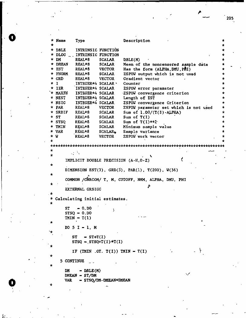
0
o
* Name Type Description * * * * DBLE INTRINSIC FONCTION * * DLOG __ INTRINSIC FUNCTION * * DM REAL*8 SCALAR QBLE(M) * * DMEAN REAL*8 SCALAR Mean of the noncensored sample dàta * * EST REAL*8 VECTOR Has the form (ALPHA,DMU,pAI) * * FNORK REAL*8 SCALAR ZSPOW output which is, not u8ed * * GRD REAL*8 VECTOR Gradient vector * * l INTEGER*4 SCALAR' Counter * * 1ER INTEGER*4 SCALAR ZSPOW error parame ter * '* MAXFN INTEGER*4 SCALAR ·ZSPOW convergence criterion * * NEST INTEGER*4 SCALAR Length of EST * ,. * NSIG INTEGER*4 SCALAR ZSPOW convergence Criterion * * PAR REAL*8 VECTOR ZSPOW parame ter set which i8 not used * * SRDIF REAL*8 SCALAR Sum of 1.~0/(T(~)-~PHA) * * ST REAL*B SCALAR Sum of T(I) * * STSQ REAL*8 SCALAR Sum of T(I)**2' * * TMIN R~L*B SCALAR Minimum sample v~lue * * VAR REAL*B SCALAR. Samp1~ variance * * loI REAL*8 VECTOR ZSPOW work vector * * * ************************************************************************ * * *
* *
" IMPLICIT DOUBLE PRECISION (A-H,O-Z)
DIMENSlON EST(3), GRD(j), PAR(l), T(200), W(36)
'" COMMON /CNRCOM/ T, M, CUTOFF, NMM, ALPHA, DHU, PHI
EXTERNAL GRSIGC St
* Calcu1ating initial estimates.
*
* '*
* * *
*
ST - O .. DO STSQ - O.DO TMIN - T(l)
DO 5 l - l, M
ST - ST+T(I) STSQ -,STSQ+T(I)*T(I)
IF (TMIN .GT. T(I» THIN - T(I)
5 CONTINUE
DM - IlBLE(M) DMEAN - ST/DM VAR - STSQjDM-DMEAN*nMEAN
205
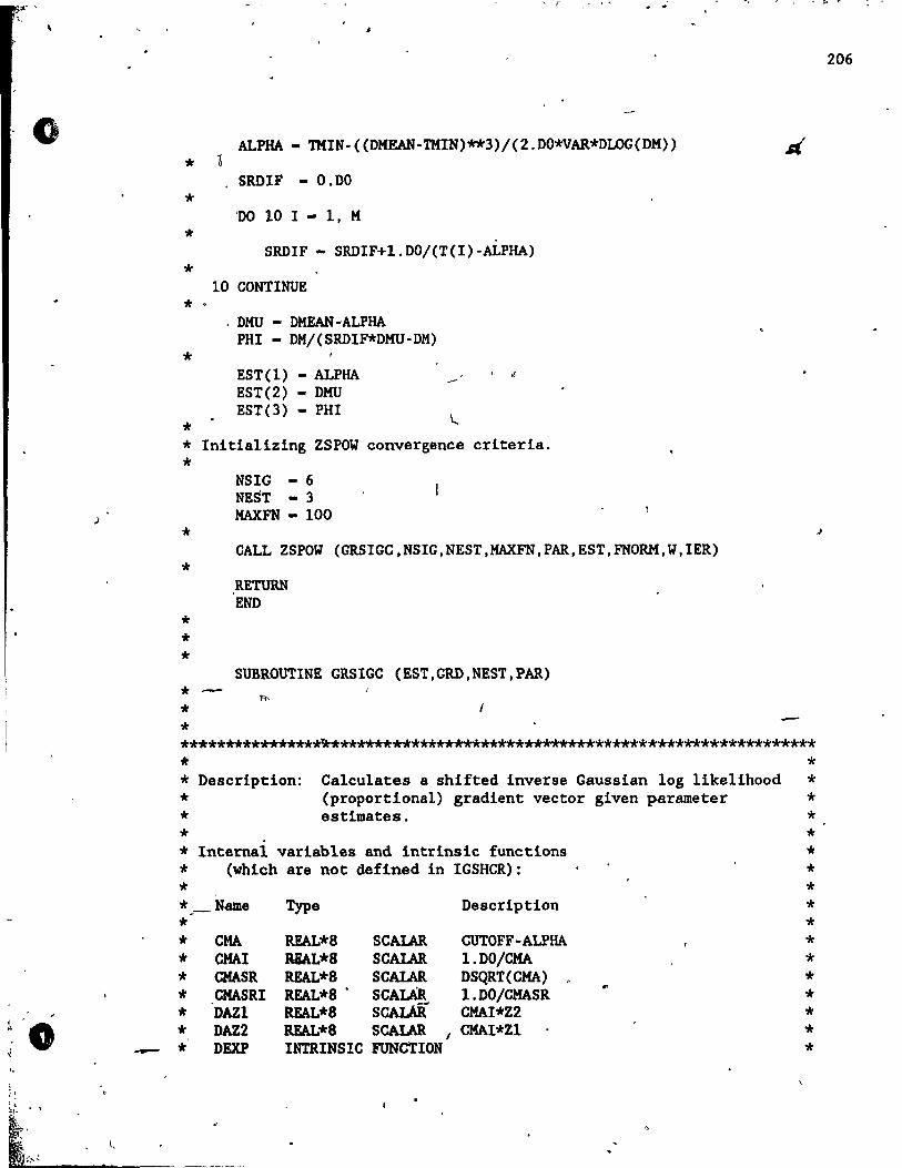
.~- . '<,
o
1.
L '.
)
\,
* '3
* *
*
ALPHA - TMIN-«DMEAN-THIN)**3)/(2.DO*VAR*DLOG(DM»
SRDIF - O.DO
'DO 10 l - l, K
SRDIF - SRDIF+1.DO/(T(I)-ALPHA)
10 CONTINUE * 0
, DMU - DKEAN -ALPHA PHI - DK/(SRDIF*DMU-DK)
* '
*
EST(l) - ALPHA EST(2) - DMU EST(3) - PHI
, .5
* Initializing ZSPOW convergence criteria.
*
* *
* * * * -* *
NSIG - 6 NE ST - 3 KAXFN - 100
CALL ZSPOW (GRSIGC,NSIG,NEST,KAXFN,PAR,EST,FNORM,W,IER)
,RETURN END
SUBROUTINE GRSIGC (EST,GRD,NEST,PAR)
-****************~*******************************************************
* * * Description: Calcula tes a shifted inverse Gaussian log likelihood * * (proportional) gradient vector given parame ter * * estimates. * * * Internal variables and intrlnsic functlons * (whlch are not defined in IGSHCR):
* * __ Name
* * * * * * *
-- *
CMA CHAI CMASR CMASRI 'DAZl DAZ2 DEXP
Type
REAL*8 SCMAR REAL*8 SCALAR REAL*8 SCALAR REAL*8' SCALAR REAL*8 SCALAR REAL*8 SCALAR 1
INTRINSIC FUNCTION
Description
CUTOFF-ALPHA l.DO/CHA DSQRT(CKA) l.DO/CMASR CMAI*Z2 CMAI*Zl
* * * * * * * * * * * * *
206
J
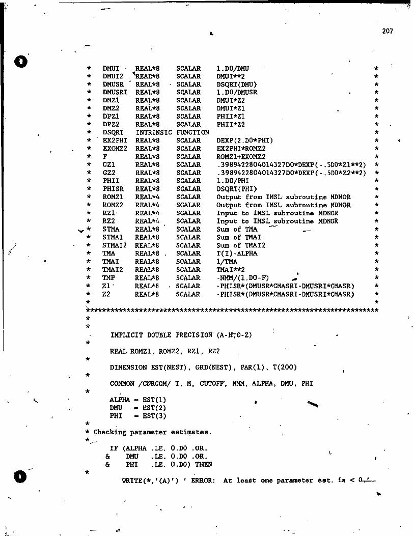
o
;/ ..
o~
* * * * * * * * * * * * * * * * * * * *
.... * * * * * * * * *
DHU 1 REAL*8 DHU 1 2 ~REAI:*8 DHUSR . REAL*8 DHUSRI REAL*8 DMZl REAL*8 DMZ2 REAL*S DPZl REAL*8 DPZ2 REAL*8 DSQRT INTRINSIC EX2PHI REAL*8 EXOMZ2 REAL*8 F REAL*8 GZl REAL*8 GZ2 REAL*8 PHIl REAL*8 PHISR REAL*8 ROMZl REAL*4 ROMZ2 REAL*4 RZl' REAL*4 RZ2 REAL*4 STMA REAL*8 STMAI REAL*8 STMAI2 REAL*8 TMA REAL*8 THAl REAL*8 !MAI 2 REAL*8 TMP REAL*8
SCAlAR SCAlAR SCAlAR SCAlAR SCAlAR SCALAR SCALAR SCAlAR F1JNCTION SCAlAR SCALAR SCALAR SCALAR SCALAR SCALAR SCALAR SCALAR SCAlAR SCALAR SCALAR SCALAR SCALAR SCAlAR SCAlAR SCALAR SCALAR SCALAR
Zl' REAL*8 Z2 REAL*8
c SCALAR SCALAR
l.DO/DHU DMUI**2 DSQRT(DMU) l.DO/DHUSR DMUI*Z2 DMUI*Zl PHIl*Zl PHII*Z2
DEXP(2.DO*PHI) EX2PHI*ROMZ2 ROMZ1+EXOMZ2 .3989422804014327DO*DEXP(-.SDO*Zl**2) .3989422804014327DO*DEXP(-.SDO*Z2**2) 1. DO/PHI DSQRT(PHI) Outp~t from IMSL' subroutlne MONOR Output from IMSL subroutine MDNOR Input to IMSL subroutine MONOR Input to IMSL subroutine MONOR Sum of TMA - ,..-Sum of TMAI Sum of !MAI2 T(I) -ALPHA l/TMA TMAI**2 -NMM/(l.DO-F) ~ -PHISR*(DMUSR*CMASRI-DMUSRI*CMASR) -PHISR*(DMUSR*PMASRI-DMUSRI*CMASR)
* * * * * * * * * * * * * * * * * * * * * * * * * * :.. * *
* * , ************************************************************************
201
* • * * *
* *
*
IMPLICIT DOUBLE PRECISION (A-~~-Z)
REAL ROMZ1, ROMZ2, RZl, RZ2
DIMENSION EST(NEST), G~(NEST), PAR(l), T(200)
COMMON /CNRCOM/ T, M, CUTOFF', NMM, ALPHA, DMU, PHI
ALPHA - EST(l) DHU - EST(2) PHI - EST(3)
,
* Checking parameter estl~ates. */""
IF (ALPHA .LE. O.DO .OR. & DHU .LE. 0.00 .OR. & PHI .LE. 0.00) THEN
* WRITE(*,'(A)') , ERROR: At least one parameter est. 18 < ~
.1 '
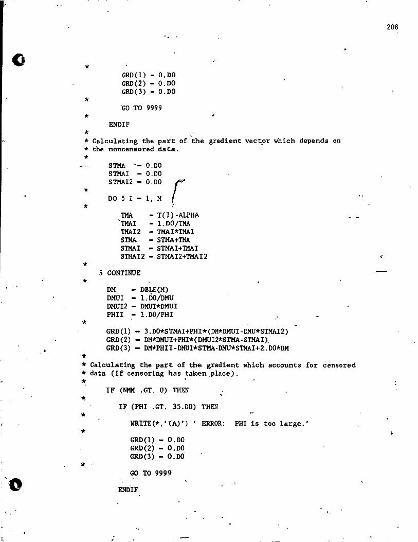
0
, .
'1
* GRD(l) - 0.00 GRD(2) - 0.00 GRD(3) - 0.00
* -GO TO 9999 *
ENDIF *
" * Calculating the part of the gradient vectpr which depends on * the noncensored data. *
* *
*
*
*
*
STMA .- O.DO STMAI - O.DO STMAI2 - O.DO
DO 5 1 - l, M r TMA - T(l)-ALPHA ~TMAI - 1. DO/TMA TMAI2 - TMAI*TMAI STMA - STMA+TMA STMAI - STMAI+TMAI STMAI2 - STMAI2+TMAI2
5 CONTINUE
DM DHU! -DMUI2 -PHIl -
DBLE(M) 1. DO;DMU DMUI*DMUI 1. DO/PHI
GRD(l) - 3.DO*STMAI~PHI*(DM*DMUI-DMU*STMAI2) GRD(2) - DM*DMUI+PHI*(DHUI2*STMA-STMAI). GRD(3) DM*PHII-DMUI*STMA-DMU*STMAI+2.DO*DM
* Calculating the part of the gradient which accounts for censored * data (if censoring has taken ,place) . * .
* *
*,
IF (NMM .GT. 0) THEN
I~ (PHI .GT. 35.DO) THEN
WRITE(*,'(A)') , ERROR:
GRD(l) - O. DO GRD(2) - 0.00 GRD(3) - O. DO
GO TO 9999
ENDIF
"
PHI is too large.'
208
'\
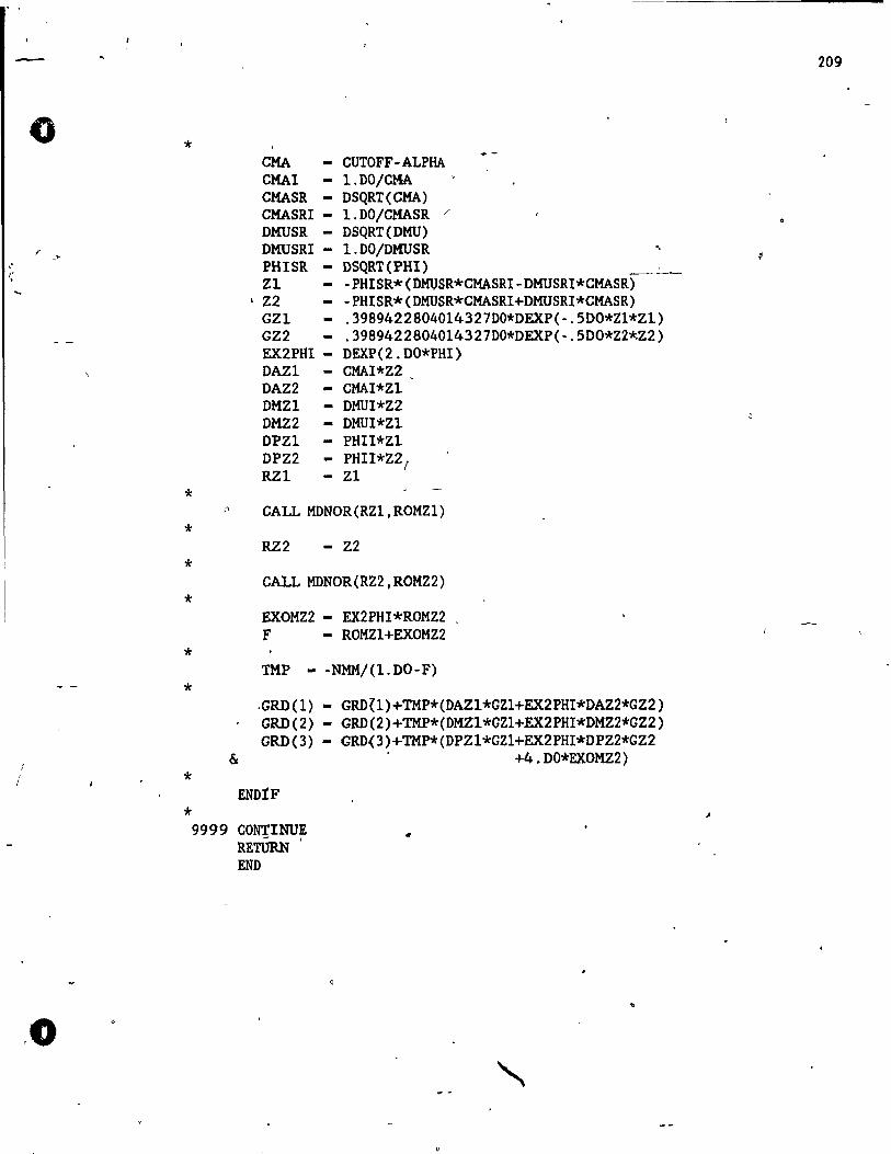
209
0 *
CMA - CUTOFF - ALPHA CMAI - 1. DOjCMA CMASR - DSQRT(CMA) CMASRI - l.DOjCMASR /
DMUSR - DSQRT(DMU) ,r DMUSRI - l.DOjDMUSR "
.'" ~ PHISR DSQRT(PHI) \ Z1 - PHISR* (OMUSR*CMASRI -DMUSRI*CMASR~) ----
• Z2 - -PHISR*(DMUSR*CMASRI+DMUSRI*CMASR) GZI - .3989422804014327DO*DEXP(-.SDO*Zl*Zl) GZ2 - .3989422804014327DO*DEXP(-.5DO*Z2~Z2)
EX2PIH - DEXP(2. DO*PHI) DAZI - CMAI*Z2 DAZ2 - CMAI*Zl DMZI - DMUI*Z2 DMZ2 - DMUI*Z1 DPZl - PHU*Z1 DPZ2 - PHII*Z2r RZl Zl
* () CALL MDNOR(RZl, ROMZl)
* RZ2 - Z2
* CALL MDNOR{RZ2,ROMZ2)
* EXOMZ2 - EX2PHI*ROMZ2 F - ROMZl+EXOMZ2
* TMP - -NMMj(l. DO-F)
* .GRD(1) - GRD{l)+TMP*(DAZl*GZl+EX2PHI*DAZ2*GZ2) GRD(2) - GRD(2)+TMP*(DMZl*GZl+EX2PHI*DMZ2*GZ2) GRD(3) - GRD{3)+TMP*(DPZl*GZl+EX2PHI*DPZ2*GZ2
1 & +4 • DO*EXOMZ2)
/ * ENDtF
* J
9999 CONTINUE .. RETÛRN 1
END
.0
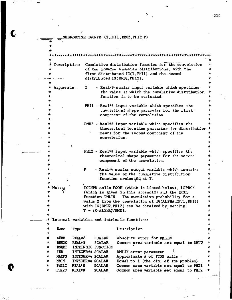
0
--===-----=~SUBROUTINE IGCNPR (T, PHIl, DMU2 , PHI2 ,P)
* *
't
* ************************************************************************ * ~/* '* Description: Cumulative distribution function for the convolution * * of two inverse Gaussian distributions, with the * * first distributed IG(I, PHIl) and the second *
~ -----* - ----- distributed IG(DMU2, PHI2). *
-------
* * * Arguments: T - Real*8- scalar input variable which specifies *
* * * * * * * * * * * * * * * * * * -* * . * * * Note~
* * * * *
the value at which the cumulative distribution * function is, to be evaluated. *
* PHIl - Real*8 input variable which specifies the *
theoretical shape parame ter for the first· * component of the convolution. *
* DMU2 - Real*8 input variable which ~pecifies the *
theoretical location parameter (or distribution * Mean) for the second component of the * convolution. *
* o * .
PHI2 - Real*8 input variable which specifies the * theoretical shape pa}:'ameter for the second * component of the convolution. *
P - Real*4 scalar output variable which contains the value of the cumulative distribution function evalua~'ê4 at T.
IGCNPR caUs FCON (which is listed below), IGPROB' (which is given in this appendix) and the IMSL function DMLIN. The cumulative probability for a value X from the convolution of IG(ALPHA,DMUl, PHIl) with IG(DMU2,PHI2) can be obtained by setting T - (X-ALPHAT/DMUl. •
* * * * * * * * * * * *
* ~==--%-j;,Internal variables and intrinsic functions: * * '!<_-
* * * * * * * * * * *
Name
AERR DMU2C DSQRT 1ER MAXFN NDIH PHllC PHl2C
Type
REAL*8 SCALAR REAL*8 SCALAR INTRINSIC FUNCTION INTEGER*4 SCALAR INTEGER*4 SCALAR INTEGER*4 SCALAR REAL*8 SCALAR REAL*8 SCALAR
Description
Absolute error for DHLIN Common area variable set equal to DMU2
DKLl~ error parame ter Approximate # of FCON caUs Equal to 1 (the dim. of the problem) Common area variable set equal to PHIl Common area variable set equa1 to PHI2
* * * * * * * * *
210
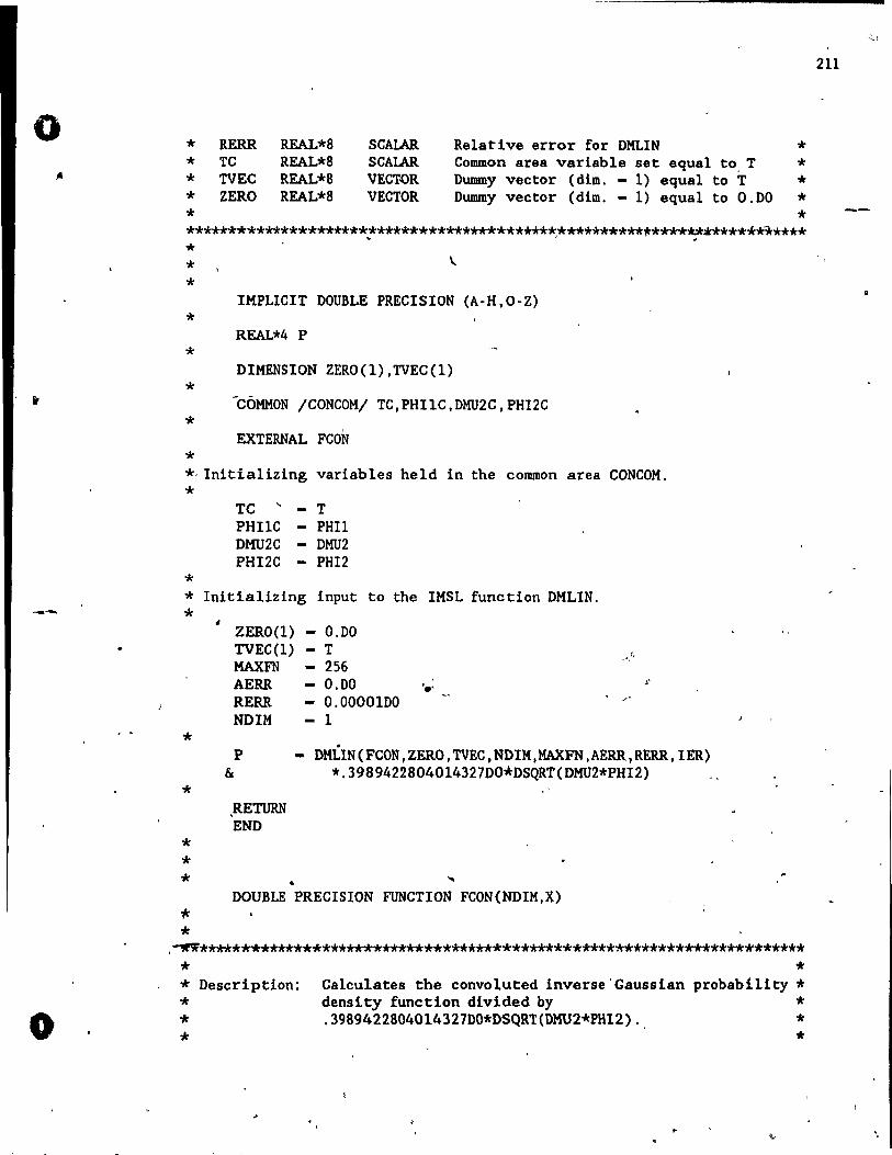
0 1&
--
o
* RERR REAL*8 SCAIAR Relative error for DHLIN * * TC REAL*8 SCAIAR Common area variable set equal to, T * * TVEC REAL*8 VECT.QR Dummy vector (dim. - 1) equal to T * * ZERO REAL*8 VECTOR Dummy vector (dim. - 1) equal to O.DO * * * *****************************************************t******~*********** * ' ~ / " * ~ *
IMPLICIT DOUBLE PRECISION (A-H,O-Z)
* REAL*4 P
* DIMENSION ZERO(I), TVEC(1)
* -COMHON /CONCOH/ TC, PHIIC, DMU2C, PHI2C
* EXTERNAL FCON
* *, Initializing variables held in the common are a CONCOH.
*
*
TC " PHllC DMU2C PHI2C
T - PHIl
DMU2 - PHI2
* Initializing input to the IHSL function DMLIN.
*
*
*
* * * "ft
*
ZERO(l) - 0.00 TVEC(1) T ," MAXFN - 256 AERR O.DO . .,. .-RERR O.OOOOlDO ,"
NDIH 1
P DHLIN(FCON,ZERO,TVEC,NDIM,HAXFN,AERR,RERR,IER) & *.3989422804014327DO*DSQRT(DHU2*PHI2)
,RETURN END
• DOUBLE PRECISION FUNCTION FCON(NDIH,X)
,~**********************************************************************
* * * Description: Calculates the convoluted inverse' Gaussian probab!lity * * density function divlded by * * . 3989422804014327DO*DSQRT(DKU2*PHI2). *
* *
211
9
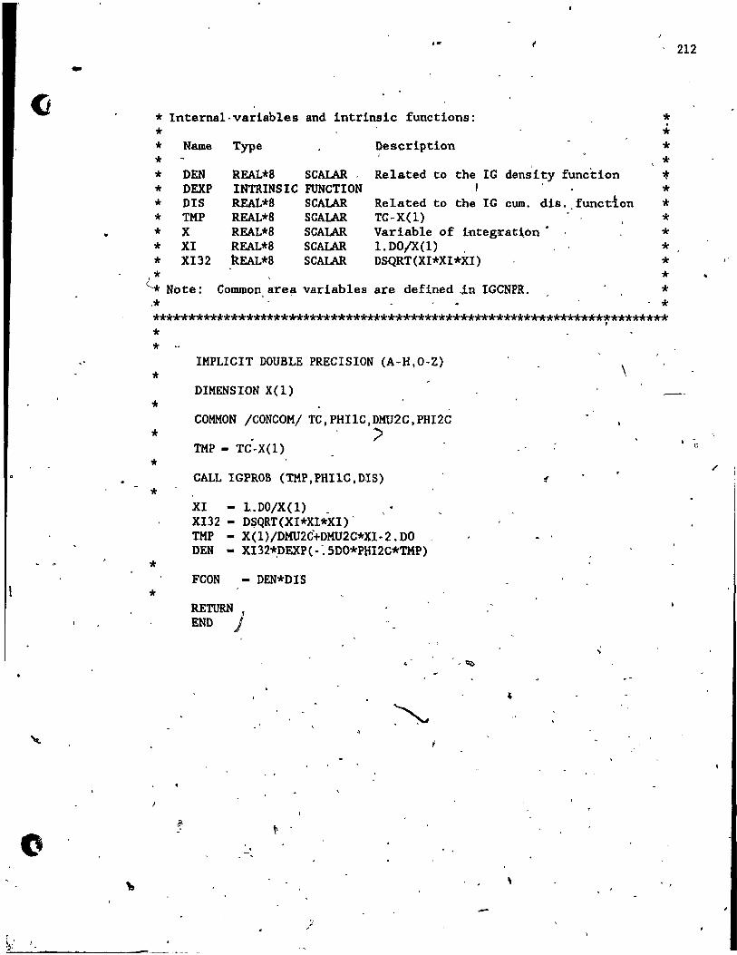
..
.'
....
* Internai·variables and intrinsic functions:
* * Name Type Description *
1
* DEN REAL*8 SCAlAR Related to the IG dens'ity function * DEXP INTRINSIC FUNCTION 1
* DIS REAL*8 SCAlAR Related to the IG cum. dis .. function * TMP REAL*8 SCAlAR TC-X(l) * X REAL*8 SCAlAR Variable of integratton . * XI REAL*8 SCALAR 1. DO/X(l) * XI32 k.EAL*8 SCALAR. DSQRT(XI*Xl*XI) * ~ Note: Common are~ variables are defined in IGCNPR. ,*
,1
* . * * *
'* * * * * * * * * *
************************************************************************ * * * * * * *
* *
IMPLICIT DOUBLE PRECISION (A-H,O-Z)
DIMENSION X(l)
COMMON /CONCOM/ TC,PHI1C,DMU2C,PHI2C . :>
TMP - TC-,X(l)
CALL IGPRO~ (TMP,PHIlC,DlS)
XI - 1.DOjX(1) _ XI32 - DSQRT(XI*Xl*XI)' TMP - X(1)/DMU2C+DMU2C*XI-2. DO DEN - XI32~DEXP(-:5DO*P"I2C*TMP)
FCON DEN*DI'S
RETURN R
END J
-' , .
•
\
(
. '
\
212
"
/
\
o
o
Statement of Originality • C
, In accordance with HcGill University thesis regulations this
, seatement outlines the elements in this thesis whi~, should be
co~sidered as, contributions to original knowled.ge. An historica1
background and, review of rè1ated works are given in the !irst , three chapters. .
This thesis represents the first cohcert~d effort to assess ~he
,usefu1ness of the inverse Gaussian di,stribution as a basis for,
statistical analyses of psychological latency data. -This included
applying est~b1ished and new methods to extensive set~ of reactioh ,
time data which were provided through the courtesy of Dr. S. L. Burbeck
and Dr. S. W. Link.
The advàntages of adding a 'shift parame ter to the distribution
definition in: the 'context of analysing 1atency data are assessed in
èhapter _4 .. The blisic properties of the three-parameter inverse
G,ussian had been previous1y investigated by Cheng and Amin (1981) and
Padgett and Wei (1981). A new algorithm for obtaining maximum.
like1ihood estimates for this case (and for the three-parameter .
lognormal) ls given. Original procedures for hand1ing Type 1 censored
and shifted inverse ,Gaussian data are also presentèd in chapter 4.
The convolution of t~o arbitrary inversè Gaussian distributions
(wlth one containing a ,shift parameter) was ,1nvestigated for the first ~ " , "
time and resu1ts are given in chapt'er 5" a10ng wit~ procedures ta , .
account for Type 1 censoring for this case. Also discussed are.
applications of this convolution to the model1ng of components of-
\
21.3
..
"
,
, '
l' 1,.,
o
1
"
reaction time. '~
'. Established la~ge smple tests are discussed in chapter 6 and
applied to ~h~_ estlmates devel~ped in chapters 4 and 5. An original
simulation study on the behavlour of shifted inverse Ga(1ssian parameterl
,estim4tes. for c~ll:sored and noncensored samples is also presented.
Six basic FORTRAN subroutines, are given in Appendix C. The,
programs. ,!GRAND and IGPROB are based on results given in Michaél, ,
Schucany, and Haas (1976), and Chan, Cohen, and wpitten (1983),
respectbrdy. The other four (i. e., IG~JlFT, LNSHFT, IGSHCR, and
\ IGCNPR) contait'l ~riginal a1gorithms.
, .
• , ,
..
. , " .
>.
, '
'.
'., '
. , " . ,
, .
.' -
, .-:
.'
214
, ' 1

![ACCESSORIOS Magnum Pistolas semiautomáticas...Lincoln Electric ® Serie LN-7, LN-8, LN-9, LN-25 [Alambre de hasta .052 pulg. (1.4 mm)] K489-1 Serie LN-8, LN-9, LN-25 [Alambre de 1/16](https://img.pdfslide.us/doc/110x75/5f37ed334803986d4a61858a/accessorios-magnum-pistolas-semiautomticas-lincoln-electric-serie-ln-7.jpg)


![LN-25 Wire Feeders Product Info - Ram Welding Supply - LN-25...LN-25 Wire Feeder | [ 3 ] key controls LN-25 PRO/LN-25 PRO eXTRa TORQUe LN-25 PRO DUaL POWeR 1. Analog Voltmeter 2. Wire](https://img.pdfslide.us/doc/110x75/5b444cec7f8b9a81058b915a/ln-25-wire-feeders-product-info-ram-welding-supply-ln-25ln-25-wire-feeder.jpg)


![Samsung Ln-s3292d Ln-s4092d Ln-s4692d Bn94-01037a Schematic Diagram [Sch]](https://img.pdfslide.us/doc/110x75/563db88d550346aa9a94b946/samsung-ln-s3292d-ln-s4092d-ln-s4692d-bn94-01037a-schematic-diagram-sch.jpg)