, Paul Fearnhead and Gareth Roberts … · The Zig-Zag Process and Super-E cient Sampling for Bayesian Analysis of Big Data Joris Bierkens 1, Paul Fearnhead 2 and Gareth Roberts 1

Submitted to the Annals of Statistics

THE ZIG-ZAG PROCESS AND SUPER-EFFICIENTSAMPLING FOR BAYESIAN ANALYSIS OF BIG DATA

By Joris Bierkens∗, Paul Fearnhead∗ and Gareth Roberts∗

Delft University of Technology, Lancaster University and University ofWarwick

Abstract Standard MCMC methods can scale poorly to big datasettings due to the need to evaluate the likelihood at each iteration.There have been a number of approximate MCMC algorithms thatuse sub-sampling ideas to reduce this computational burden, but withthe drawback that these algorithms no longer target the true poste-rior distribution. We introduce a new family of Monte Carlo meth-ods based upon a multi-dimensional version of the Zig-Zag process ofBierkens and Roberts (2017), a continuous time piecewise determinis-tic Markov process. While traditional MCMC methods are reversibleby construction (a property which is known to inhibit rapid conver-gence) the Zig-Zag process offers a flexible non-reversible alternativewhich we observe to often have favourable convergence properties. Weshow how the Zig-Zag process can be simulated without discretisationerror, and give conditions for the process to be ergodic. Most impor-tantly, we introduce a sub-sampling version of the Zig-Zag processthat is an example of an exact approximate scheme, i.e. the resultingapproximate process still has the posterior as its stationary distri-bution. Furthermore, if we use a control-variate idea to reduce thevariance of our unbiased estimator, then the Zig-Zag process can besuper-efficient: after an initial pre-processing step, essentially inde-pendent samples from the posterior distribution are obtained at acomputational cost which does not depend on the size of the data.

1. Introduction. The importance of Markov chain Monte Carlo tech-niques in Bayesian inference shows no signs of diminishing. However, allcommonly used methods are variants on the Metropolis-Hastings (MH) algo-rithm (Metropolis et al., 1953; Hastings, 1970) and rely on innovations whichdate back over 60 years. All MH algorithms simulate realisations from a dis-crete reversible ergodic Markov chain with invariant distribution π whichis (or is closely related to) the target distribution, i.e. the posterior distri-bution in a Bayesian context. The MH algorithm gives a beautifully simple

∗The authors acknowledge the EPSRC for support under grants EP/D002060/1(CRiSM) and EP/K014463/1 (iLike).

MSC 2010 subject classifications: Primary 65C60; secondary 65C05, 62F15, 60J25Keywords and phrases: MCMC, non-reversible Markov process, piecewise deterministic

Markov process, Stochastic Gradient Langevin Dynamics, sub-sampling, exact sampling

1imsart-aos ver. 2014/10/16 file: zigzag-arXiv-v2.tex date: April 24, 2018

arX

iv:1

607.

0318

8v2

[st

at.C

O]

23

Apr

201

8

http://www.imstat.org/aos/

2 J. BIERKENS, P. FEARNHEAD AND G. O. ROBERTS

though flexible recipe for constructing such Markov chains, requiring onlylocal information about π (typically pointwise evaluations of π and, perhaps,its derivative at the current and proposed new locations) to complete eachiteration.

However new complex modelling and data paradigms are seriously chal-lenging these established methodologies. Firstly, the restriction of traditionalMCMC to reversible Markov chains is a serious limitation. It is now well-understood both theoretically (Hwang, Hwang-Ma and Sheu, 1993; Chenand Hwang, 2013; Rey-Bellet and Spiliopoulos, 2015; Bierkens, 2015; Dun-can, Lelievre and Pavliotis, 2016) and heuristically (Neal, 1998) that non-reversible chains offer potentially massive advantages over reversible counter-parts. The need to escape reversibility, and create momentum to aid mixingthroughout the state space is certainly well-known, and motivates a num-ber of modern MCMC methods, including the popular Hamiltonian MCMC(Duane et al., 1987).

A second major obstacle to the application of MCMC for Bayesian in-ference is the need to process potentially massive data-sets. Since MH al-gorithms in their pure form require a likelihood evaluation – and thus pro-cessing the full data-set – at every iteration, it can be impractical to carryout large numbers of MH iterations. This has led to a range of alterna-tives that use sub-samples of the data at each iteration (Welling and Teh,2011; Maclaurin and Adams, 2014; Ma, Chen and Fox, 2015; Quiroz, Villaniand Kohn, 2015), or that partition the data into shards, run MCMC oneach shard, and then attempt to combine the information from these dif-ferent MCMC runs (Neiswanger, Wang and Xing, 2013; Scott et al., 2016;Wang and Dunson, 2013; Li, Srivastava and Dunson, 2017). However mostof these methods introduce some form of approximation error, so that thefinal sample will be drawn from some approximation to the posterior, andthe quality of the approximation can be impossible to evaluate. As an ex-ception the Firefly algorithm (Maclaurin and Adams, 2014) samples fromthe exact distribution of interest (but see the comment below).

This paper introduces the multi-dimensional Zig-Zag sampling algorithm(ZZ) and its variants. These methods overcome the restrictions of the liftedMarkov chain approach of Turitsyn, Chertkov and Vucelja (2011) as they donot depend on the introduction of momentum generating quantities. Theyare also amenable to the use of sub-sampling ideas. The dynamics of theZig-Zag process depends on the target distribution through the gradientof the logarithm of the target. For Bayesian applications this is a sum,and is easy to estimate unbiasedly using sub-sampling. Moreover, Zig-Zagwith Sub-Sampling (ZZ-SS) retains the exactness of the required invariant

imsart-aos ver. 2014/10/16 file: zigzag-arXiv-v2.tex date: April 24, 2018

ZIG-ZAG SAMPLING 3

distribution. Furthermore, if we also use control variate ideas to reduce thevariance of our sub-sampling estimator of the gradient, the resulting Zig-Zag with Control Variates (ZZ-CV) algorithm has remarkable super-efficientscaling properties for large data sets.

We will call an algorithm super-efficient if it is able to generate inde-pendent samples from the target distribution at a higher efficiency than ifwe would draw independently from the target distribution at the cost ofevaluating all data. The only situation we are aware of where we can im-plement super-efficient sampling is with simple conjugate models, where thelikelihood function has a low-dimensional summary statistic which can beevaluated at cost O(n), where n is the number of observations, after whichwe can obtain independent samples from the posterior distribution at a costof O(1) by using the functional form of the posterior distribution. The ZZ-CV can replicate this computational efficiency: after a pre-computation ofO(n), we are able to obtain independent samples at a cost of O(1). In thissense it contrasts with the Firefly algorithm (Maclaurin and Adams, 2014)which has an ESS per datum which decreases approximately as 1/n wheren is the size of the data, so that the gains of this algorithm do not increasewith n; see (Bouchard-Cote, Vollmer and Doucet, 2015, Section 4.6).

This breakthrough is based upon the Zig-Zag process, a continuous timepiecewise deterministic Markov process (PDMP). Given a d-dimensionaldifferentiable target density π, Zig-Zag is a continuous-time non-reversiblestochastic process with continuous, piecewise linear trajectories on Rd. Itmoves with constant velocity, Θ ∈ {−1, 1}d, until one of the velocity compo-nents switches sign. The event time and choice of which direction to reverse iscontrolled by a collection of state-dependent switching rates, (λi)

di=1 which

in turn are constrained via an identity (2) which ensures that π is a sta-tionary distribution for the process. The process intrinsically is constructedin continuous-time, and it can be easily simulated using standard Poissonthinning arguments as we shall see in Section 3.

The use of PDMPs such as the Zig-Zag processes is an exciting andmostly unexplored area in MCMC. The first occurrence of a PDMP forsampling purposes is in the computational physics literature (Peters and DeWith, 2012), which in one dimension coincides with the Zig-Zag process. InBouchard-Cote, Vollmer and Doucet (2015) this method is given the nameBouncy Particle Sampler. In multiple dimensions the Zig-Zag process andBouncy Particle Sampler (BPS) are different processes: both are PDMPswhich move along straight line segments, but the Zig-Zag process changesdirection in only a single component at each switch, whereas the BouncyParticle Sampler reflects the full direction vector in the level curves of the



density function. As we will see in Section 2.4, this difference has a beneficialeffect on the ergodic properties of the Zig-Zag process. The one-dimensionalZig-Zag process is analysed in detail in e.g. Fontbona, Guerin and Malrieu(2012); Monmarche (2014); Fontbona, Guerin and Malrieu (2016); Bierkensand Roberts (2017).

Since the first version of this paper was conceived already several otherrelated theoretical and methodological papers have appeared. In particularwe mention here results on exponential ergodicity of the BPS (Deligiannidis,Bouchard-Cote and Doucet, 2017) and ergodicity of the multi-dimensionalZig-Zag process (Bierkens, Roberts and Zitt, 2017). The Zig-Zag processhas the advantage that it is ergodic under very mild conditions, which inparticular means that we are not required to choose a refreshment rate. Atthe same time, the BPS seems more ‘natural’, in that it tries to minimisethe bounce rate and the change in direction at bounces, and it may bemore efficient for this reason. However it is a challenge to make a directcomparison in efficiency of the two methods since the efficiency dependsboth on the computational effort per unit of continuous time of the respectivealgorithms, as well as the mixing time of the underlying processes. Thereforewe expect analysing the relative efficiency of PDMP based algorithms to bean important area of continued research for years to come.

A continuous-time sequential Monte Carlo algorithm for scalable Bayesianinference with big data, the SCALE algorithm, is given in Pollock et al.(2016). Advantages that Zig-Zag has over SCALE is that it avoids the issueof controlling the stability of importance weights, and it is simpler to imple-ment. Whereas the SCALE algorithm is well-adapted for the use of parallelarchitecture computing, and has particularly simple scaling properties forbig data.

1.1. Notation. For a topological space X let B(X) denote the Borel σ-algebra. We write R+ := [0,∞). If h : Rd → R is differentiable then ∂ih

denotes the function ξ 7→ ∂h(ξ)∂ξi

. We equip E := Rd × {−1,+1}d with the

product topology of the Euclidean topology on Rd and the discrete topologyon {−1,+1}d. Elements in E will often be denoted by (ξ, θ) with ξ ∈ Rdand θ ∈ {−1,+1}d. For g : E → R differentiable in its first argument we

will use ∂ig to denote the function (ξ, θ) 7→ ∂g(ξ,θ)∂ξi

, i = 1, . . . , d.

2. The Zig-Zag process. The Zig-Zag process is a continuous timeMarkov process whose trajectories lie in the space E = Rd×{−1,+1}d andwill be denoted by (Ξ(t),Θ(t))t≥0. They can be described as follows: at ran-dom times a single component of Θ(t) flips. In between these switches, Ξ(t)


ZIG-ZAG SAMPLING 5

is linear with ddtΞ(t) = Θ(t). The rates at which the flips in Θ(t) occur are

time inhomogeneous: the i-th component of Θ switches at rate λi(Ξ(t),Θ(t)),where λi : E → R+ for i = 1, . . . , d are continuous functions.

2.1. Construction. For a given (ξ, θ) ∈ E, we may construct a trajectoryof (Ξ,Θ) of the Zig-Zag process with initial condition (ξ, θ) as follows.

• Let (T 0,Ξ0,Θ0) := (0, ξ, θ).• For k = 1, 2, . . .

– Let ξk(t) := Ξk−1 + Θk−1t, t ≥ 0

– For i = 1, . . . , d, let τki be distributed according to

P(τki ≥ t) = exp

(−∫ t

0λi(ξ

k(s),Θk−1) ds

).

– Let i0 := argmini∈{1,...,d} τki and let T k := T k−1 + τki0 .

– Let Ξk := ξk(T k).

– Let

Θk(i) :=

{Θk−1(i) if i 6= i0,−Θk−1(i) if i = i0

This procedure defines a sequence of skeleton points (T k,Ξk,Θk)∞k=0 in R+×E, which correspond to the time and position at which the direction of theprocess changes. The trajectory ξk(t) represents the position of the processat time T k−1 + t until time T k, for 0 ≤ t ≤ T k − T k−1. The time until thenext skeleton event is characterized as the smallest time of a set of eventsin d simultaneous point processes, where each point process correspondsto switching of a different component of the velocity. For the i-th of theseprocesses, events occur at rate λi(ξ

k(s),Θk−1), and τki is defined to be thetime to the first event for the i-th component. The component for which theearliest event occurs is i0. This defines τki0 , the time between the (k − 1)thand kth skeleton point, and the component, i0, of the velocity that switches.

The piecewise deterministic trajectories (Ξ(t),Θ(t)) are now obtained as

(Ξ(t),Θ(t)) := (Ξk + Θk(t− T k),Θk) for t ∈ [T k, T k+1), k = 0, 1, 2, . . . .

Since the switching rates are continuous and hence bounded on compactsets, and Ξ will travel a finite distance within any finite time interval, withinany bounded time interval there will be finitely many switches almost surely.

The above procedure provides a mathematical construction of a Markovprocess as well as the outline of an algorithm which simulates this process.



The only step in this procedure which presents a computational challenge isthe simulation of the random times (T ki ) and a significant part of this paperwill consider obtaining these in a numerically efficient way.

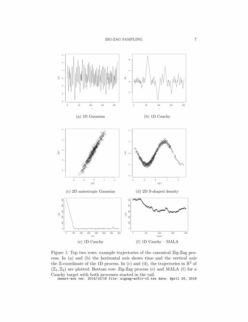
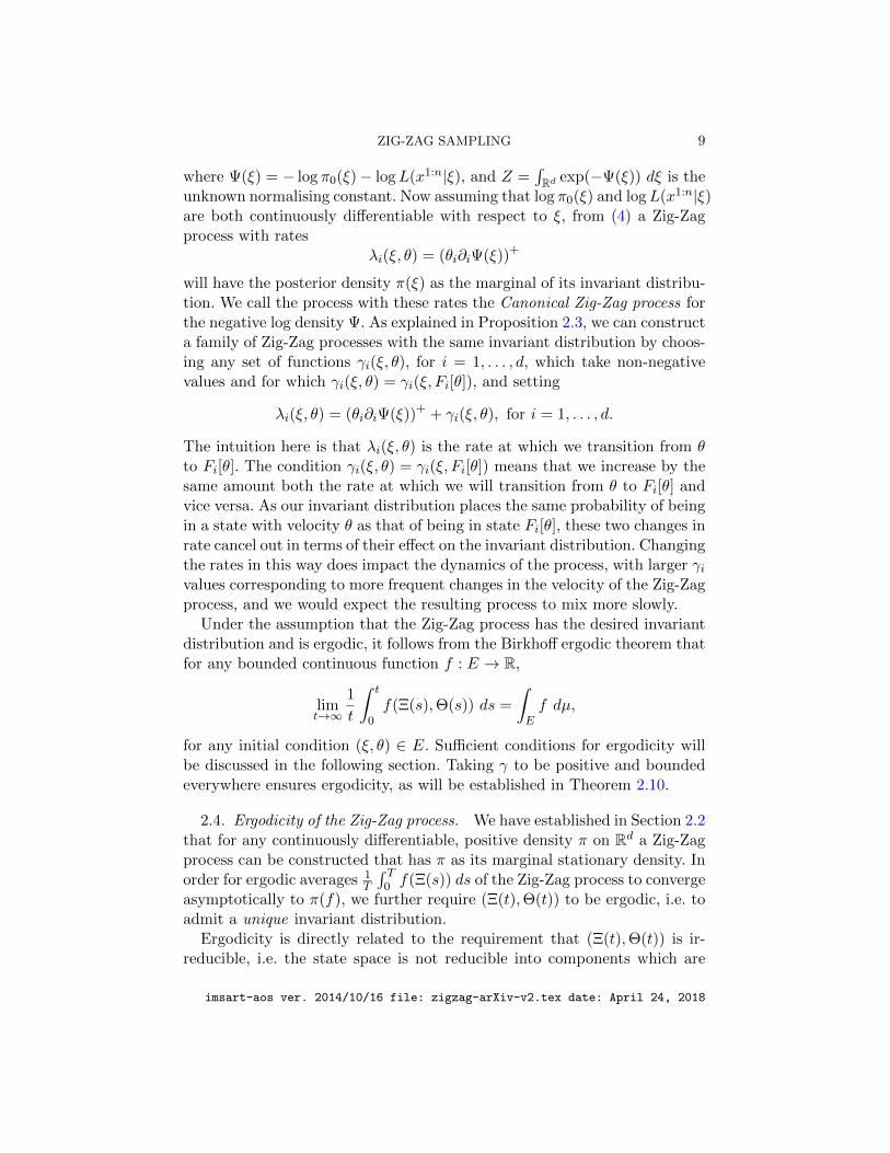
Figure 1 displays trajectories of the Zig-Zag process for several examplesof invariant distributions. The name of the process is derived by the zig-zagnature of paths that the process produces. Figure 1 shows an important dif-ference in the output of the Zig-Zag process, as compared to a discrete-timeMCMC algorithm: the output of is a continuous-time sample path. The bot-tom row of plots in Figure 1 also gives a comparison to a reversible MCMCalgorithm, Metropolis Adjusted Langevin (MALA Roberts and Tweedie,1996), and demonstrates an advantage of a non-reversible sampler: it cancope better with a heavy tailed target. This is most easily seen if we startthe process out in the tail, as in the figure. The velocity component of theZig-Zag process enables it to quickly return to the mode of the distribution,whereas the reversible algorithm behaves like a random walk in the tails,and takes much longer to return to the mode.

2.2. Invariant distribution. The most important aspect of the Zig-Zagprocess is that in many cases the switching rates are directly related toan easily identifiable invariant distribution. Let C1(Rd) denote the spaceof continuously differentiable functions on Rd. For θ ∈ {−1,+1}d and i ∈{1, . . . , d}, let Fi[θ] ∈ {−1,+1}d denote the binary vector obtained by flip-ping the i-th component of θ; i.e.

(Fi[θ])j =

{θj if i 6= j,

−θj if i = j..

We introduce the following assumption.

Assumption 2.1. For some function Ψ ∈ C1(Rd) satisfying

(1)

∫Rd

exp(−Ψ(ξ)) dξ <∞

we have

(2) λi(ξ, θ)− λi(ξ, Fi[θ]) = θi∂iΨ(ξ) for all (ξ, θ) ∈ E, i = 1, . . . , d.

Throughout this paper we will refer to Ψ as the negative log density. Letµ0 denote the measure on B(E) such that, for A ∈ B(Rd) and θ ∈ {−1,+1}d,µ0(A× {θ}) = Leb(A), with Leb denoting Lebesgue measure on Rd.


ZIG-ZAG SAMPLING 7

0 50 100 150 200

−3

−2

−1

01

23

t

Ξ(t)

(a) 1D Gaussian

0 50 100 150 200

−5

05

10

t

Ξ(t)

(b) 1D Cauchy

−2 −1 0 1 2

−2

−1

01

2

Ξ1(t)

Ξ 2(t)

(c) 2D anisotropic Gaussian

−2 −1 0 1 2

−2

−1

01

2

Ξ1(t)

Ξ 2(t)

(d) 2D S-shaped density

0 500 1000 1500 2000 2500 3000 3500

010

020

030

040

050

0

Time

Ξ 1(t)

(e) 1D Cauchy

0 500 1000 1500 2000

010

020

030

040

050

0

Iteration

Ξ 1(t)

(f) 1D Cauchy – MALA

Figure 1: Top two rows: example trajectories of the canonical Zig-Zag pro-cess. In (a) and (b) the horizontal axis shows time and the vertical axisthe Ξ-coordinate of the 1D process. In (c) and (d), the trajectories in R2 of(Ξ1,Ξ2) are plotted. Bottom row: Zig-Zag process (e) and MALA (f) for aCauchy target with both processes started in the tail.



Theorem 2.2. Suppose Assumption 2.1 holds. Let µ denote the proba-bility distribution on E such that µ has Radon-Nikodym derivative

(3)dµ

dµ0(ξ, θ) =

exp(−Ψ(ξ))

Z, (ξ, θ) ∈ E,

where Z =∫E exp(−Ψ) dµ0. Then the Zig-Zag process (Ξ,Θ) with switching

rates (λi)di=1 has invariant distribution µ.

The proof is located in the Section 1 of the Supplementary Material. Wesee that under the invariant distribution of the Zig-Zag process, ξ and θare independent, with ξ having density proportional to exp(−Ψ(ξ)) and θhaving a uniform distribution on the points in {−1,+1}d.

For a ∈ R, let (a)+ := max(0, a) and (a)− := max(0,−a) denote thepositive and negative parts of a, respectively. We will often use the trivialidentity a = (a)+−(a)− without comment. The following result characterizesthe switching rates for which (2) holds.

Proposition 2.3. Suppose λ : E → Rd+ is continuous. Then Assump-tion 2.1 is satisfied if and only if there exists a continuous function γ : E →Rd+ such that for all i = 1, . . . , d and (ξ, θ) ∈ E, γi(ξ, θ) = γi(ξ, Fi[θ]) and,for Ψ ∈ C1(Rd) satisfying (1),

(4) λi(ξ, θ) = (θi∂iΨ(ξ))+ + γi(ξ, θ).

The proof is located in Section 1 of the Supplementary Material.

2.3. Zig-Zag process for Bayesian inference. One application of the Zig-Zag process is as an alternative to MCMC for sampling from posterior dis-tributions in Bayesian statistics. We show here that it is straightforward toderive a class of Zig-Zag processes that have a given posterior distributionas their invariant distribution. The dynamics of the Zig-Zag process only de-pend on knowing the posterior density up to a constant of proportionality.

To keep notation consistent with that used for the Zig-Zag process, letξ ∈ Rd denote a vector of continuous parameters. We are given a priordensity function for ξ, which we denote by π0(ξ), and observations x1:n =(x1, . . . , xn). Our model for the data defines a likelihood function L(x1:n|ξ).Thus the posterior density function is

π(ξ) ∝ π0(ξ)L(x1:n|ξ).

We can write π(ξ) in the form of the previous section,

π(ξ) =1

Zexp(−Ψ(ξ)), ξ ∈ Rd,


ZIG-ZAG SAMPLING 9

where Ψ(ξ) = − log π0(ξ)− logL(x1:n|ξ), and Z =∫Rd exp(−Ψ(ξ)) dξ is the

unknown normalising constant. Now assuming that log π0(ξ) and logL(x1:n|ξ)are both continuously differentiable with respect to ξ, from (4) a Zig-Zagprocess with rates

λi(ξ, θ) = (θi∂iΨ(ξ))+

will have the posterior density π(ξ) as the marginal of its invariant distribu-tion. We call the process with these rates the Canonical Zig-Zag process forthe negative log density Ψ. As explained in Proposition 2.3, we can constructa family of Zig-Zag processes with the same invariant distribution by choos-ing any set of functions γi(ξ, θ), for i = 1, . . . , d, which take non-negativevalues and for which γi(ξ, θ) = γi(ξ, Fi[θ]), and setting

λi(ξ, θ) = (θi∂iΨ(ξ))+ + γi(ξ, θ), for i = 1, . . . , d.

The intuition here is that λi(ξ, θ) is the rate at which we transition from θto Fi[θ]. The condition γi(ξ, θ) = γi(ξ, Fi[θ]) means that we increase by thesame amount both the rate at which we will transition from θ to Fi[θ] andvice versa. As our invariant distribution places the same probability of beingin a state with velocity θ as that of being in state Fi[θ], these two changes inrate cancel out in terms of their effect on the invariant distribution. Changingthe rates in this way does impact the dynamics of the process, with larger γivalues corresponding to more frequent changes in the velocity of the Zig-Zagprocess, and we would expect the resulting process to mix more slowly.

Under the assumption that the Zig-Zag process has the desired invariantdistribution and is ergodic, it follows from the Birkhoff ergodic theorem thatfor any bounded continuous function f : E → R,

limt→∞

1

t

∫ t

0f(Ξ(s),Θ(s)) ds =

∫Ef dµ,

for any initial condition (ξ, θ) ∈ E. Sufficient conditions for ergodicity willbe discussed in the following section. Taking γ to be positive and boundedeverywhere ensures ergodicity, as will be established in Theorem 2.10.

2.4. Ergodicity of the Zig-Zag process. We have established in Section 2.2that for any continuously differentiable, positive density π on Rd a Zig-Zagprocess can be constructed that has π as its marginal stationary density. Inorder for ergodic averages 1

T

∫ T0 f(Ξ(s)) ds of the Zig-Zag process to converge

asymptotically to π(f), we further require (Ξ(t),Θ(t)) to be ergodic, i.e. toadmit a unique invariant distribution.

Ergodicity is directly related to the requirement that (Ξ(t),Θ(t)) is ir-reducible, i.e. the state space is not reducible into components which are



each invariant for the process (Ξ(t),Θ(t)). For the one-dimensional Zig-Zagprocess, (exponential) ergodicity has already been established under mildconditions (Bierkens and Roberts, 2017). As we discuss below, irreducibility,and thus ergodicity, can be established for large classes of multi-dimensionaltarget distributions, such as i.i.d. Gaussian distributions, and also if theswitching rates λi(ξ, θ) are positive for all i = 1, . . . , d, and (ξ, θ) ∈ E.

Let P t((ξ, θ), ·) be the transition kernel of the Zig-Zag process with initialcondition (ξ, θ). A function f : E → R is called norm-like if lim‖ξ‖→∞ f(ξ, θ) =

∞ for all θ ∈ {−1,+1}d. Let ‖ · ‖TV denote the total variation norm on thespace of signed measures. First we consider the one-dimensional case.

Assumption 2.4. Suppose d = 1 and there exists ξ0 > 0 such that

(i) infξ≥ξ0 λ(ξ,+1) > supξ≥ξ0 λ(ξ,−1), and(ii) infξ≤−ξ0 λ(ξ,−1) > supξ≤−ξ0 λ(ξ,+1).

Proposition 2.5. (Bierkens and Roberts, 2017, Theorem 5) SupposeAssumption 2.4 holds. Then there exists a function f : E → [1,∞) which isnorm-like such that the Zig-Zag process is f -exponentially ergodic, i.e. thereexists a constant κ > 0 and 0 < ρ < 1 such that

‖P t((ξ, θ), ·)− π‖TV ≤ κf(ξ, θ)ρt for all (ξ, θ) ∈ E and t ≥ 0.

Example 2.6. As an example of fundamental importance, which willalso be used in the proof of Theorem 2.10, consider a one-dimensional Gaus-

sian distribution. For simplicity let π(ξ) be centred, π(ξ) = 1√2πσ2

exp(− ξ2

2σ2

)for some σ > 0. According to (4) the switching rates take the form

λ(ξ, θ) =(θξ/σ2

)++ γ(ξ), (ξ, θ) ∈ E.

As long as γ is bounded from above, Assumption 2.4 is satisfied. In particularthis holds if γ is equal to a non-negative constant.

Remark 2.7. We say a probability density function π is of product formif π(ξ) =

∏di=1 πi(ξi), where πi : Rd → (0,∞) are one-dimensional probabil-

ity density functions. When its target density is of product form the Zig-Zagprocess is the concatenation of independent Zig-Zag processes. In this casethe negative log density is of the form Ψ(ξ) =

∑di=1 Ψi(ξi) and the switching

rate for the i-th component of θ is

(5) λi(ξ, θ) =(θiΨ

′i(ξi)

)++ γi(ξ).


ZIG-ZAG SAMPLING 11

As long as γi(ξ) = γi(ξi), i.e. if γi(ξ) only depends on the i-th coordinate of ξ,the switching rate of coordinate i is independent of the other coordinates ξj ,j 6= i. It follows that the switches of the i-th coordinate can be generated by aone-dimensional time inhomogeneous Poisson process, which is independentof the switches in the other coordinates. As a consequence the d-dimensionalZig-Zag process (Ξ(t),Θ(t)) = (Ξ1(t), . . . ,Ξd(t),Θ

1(t), . . . ,Θd(t)) consists ofa combination of d independent Zig-Zag processes (Ξi(t),Θi(t)), i = 1, . . . , d.

Suppose P (x, dy) is the transition kernel of a Markov chain on a statespace E. We say that the Markov chain associated to P is mixing if thereexists a probability distribution π on E such that

limk→∞

‖P k(x, ·)− π‖TV = 0 for all x ∈ E.

For any continuous time Markov process with family of transition kernelsP t(x, dy) we can consider the associated time-discretized process, which is aMarkov chain with transition kernel Q(x, dy) := P δ(x, dy) for a fixed δ > 0.The value of δ will be of no significance in our use of this construction.

Proposition 2.8. Suppose π is of product form and λ : E → Rd+ ad-mits the representation (5) with γi(ξ) only depending on {ξi, i = 1, . . . , d}.Furthermore suppose that for every i = 1, . . . , d, the one-dimensional time-discretized Zig-Zag process corresponding to switching rate λi is mixing inR×{−1,+1}. Then the time-discretized d-dimensional Zig-Zag process withswitching rates (λi) is mixing. In particular, the multi-dimensional Zig-Zagprocess admits a unique invariant distribution.

Proof. This follows from the decomposition of the d-dimensional Zig-Zag process as d one-dimensional Zig-Zag processes and Lemma 1.1 in theSupplementary material.

Example 2.9. Continuing Example 2.6, consider the simple case inwhich π is of product form with each πi a centered Gaussian density func-tion with variance σ2

i . It follows from Proposition 2.8 and Example 2.6 thatthe multi-dimensional canonical Zig-Zag process (i.e. the Zig-Zag processwith γi ≡ 0) is mixing. This is different from the Bouncy Particle Sampler(Bouchard-Cote, Vollmer and Doucet, 2015), which is not ergodic for ani.i.d. Gaussian without ‘refreshments’ of the momentum variable.

We now show that strict positivity of the rates ensures ergodicity.



Theorem 2.10. Suppose λ : E → (0,∞)d, in particular λi(ξ, θ) is pos-itive for all i = 1, . . . , d and (ξ, θ) ∈ E. Then there exists at most a singleinvariant measure for the Zig-Zag process with switching rate λ.

The proof of this result consists of a Girsanov change of measure withrespect to a Zig-Zag process targeting an i.i.d. standard normal distribution,which we know to be irreducible. The irreducibility then carries over to theZig-Zag process with the stated switching rates. A detailed proof can befound in the Supplementary material.

Remark 2.11. Based on numerous experiments, we conjecture that thecanonical multi-dimensional Zig-Zag process is ergodic in general under onlymild conditions. A detailed investigation of ergodicity will be the subject ofa forthcoming paper (Bierkens, Roberts and Zitt, 2017).

3. Implementation. As mentioned earlier, the main computationalchallenge is an efficient simulation of the random times T ki introduced inSection 2.1. We will focus on simulation by means of Poisson thinning.

Proposition 3.1 (Poisson thinning, Lewis and Shedler (1979)). Let m :R+ → R+ and M : R+ → R+ be continuous such that m(t) ≤ M(t) fort ≥ 0. Let τ1, τ2, . . . be the increasing finite or infinite sequence of points ofa Poisson process with rate function (M(t))t≥0. For all i, delete the pointτ i with probability 1 −m(τ i)/M(τ i). Then the remaining points, τ1, τ2, . . .say, form a non-homogeneous Poisson process with rate function (m(t))t≥0.

Now for a given initial point (ξ, θ) ∈ E, let mi(t) := λi(ξ + θt, θ), fori = 1, . . . , d, and suppose we have available continuous functions Mi(t) suchthat mi(t) ≤ Mi(t) for i = 1, . . . , d and t ≥ 0. We call these (Mi)

di=1 com-

putational bounds for (mi)di=1. We can use Proposition 3.1 to obtain the

first switching times (τ1i )di=1 from a (theoretically infinite) collection of pro-

posed switching times (τ1i , τ

2i , . . . )

di=1 given the initial point (ξ, θ), and use

the obtained skeleton point at time τ1 := mini∈{1,...,d} τ1i as a new initial

point (which is allowed by the strong Markov property) with the compo-nent i0 = argmini∈{1,...,d} τ

1i of θ switched.

The strong Markov property of the Zig-Zag process simplifies the compu-tational procedure further: we can draw for each component i = 1, . . . , d thefirst proposed switching time τi := τ1

i , determine i0 := argmini∈{1,...,d} τi anddecide whether the appropriate component of θ is switched at this time withprobability mi0(τ)/Mi0(τ), where τ := τi0 . Then since τ is a stopping timefor the Markov process, we can use the obtained point of the Zig-Zag process


ZIG-ZAG SAMPLING 13

at time τ as new starting point, regardless of whether we switch a compo-nent of θ at the obtained skeleton point. A full computational procedure forsimulating the Zig-Zag process is given by Algorithm 1.

Algorithm 1: Zig-Zag Sampling (ZZ)

Input: initial condition (ξ, θ) ∈ E.Output: a sequence of skeleton points (T k,Ξk,Θk)∞k=0.

1. (T 0,Ξ0,Θ0) := (0, ξ, θ).

2. for k = 1, 2, . . .

(a) Define mi(t) := λi(Ξk−1 + Θk−1t,Θk−1) for t ≥ 0 and i = 1, . . . , d.

(b) For i = 1, . . . , d, let (Mi) denote computational bounds for (mi).

(c) Draw τ1, . . . , τd such that P (τi ≥ t) = exp(−∫ t

0Mi(s) ds

).

(d) i0 := argmini=1,...,d{τi} and τ := τi0 .

(e) (T k,Ξk) := (T k−1 + τ,Ξk−1 + Θk−1τ)

(f) With probability mi0(τ)/Mi0(τ),

• Θk := Fi0 [Θk−1],

otherwise

• Θk := Θk−1.

3.1. Computational bounds. We now come to the important issue of ob-taining computational bounds for the Zig-Zag Process, i.e. useful upperbounds for the switching rates (mi). If we can compute the inverse functionGi(y) := inf{t ≥ 0 : Hi(t) ≥ y} of Hi : t 7→

∫ t0 Mi(s) ds, we can simulate

τ1, . . . , τd using the CDF inversion technique, i.e. by drawing i.i.d. uniformrandom variables U1, . . . , Ud and setting τi := Gi(− logUi), i = 1, . . . d.

Let us ignore the subscript i for a moment. Examples of computationalbounds are piecewise affine bounds of the form M : t 7→ (a + bt)+, witha, b ∈ R, and the constant bounds M : t 7→ c for c ≥ 0. It is also possible tosimulate using the combined rate M : t 7→ min(c, (a+ bt)+). In these cases,H(t) =

∫ t0 M(s) ds is piecewise linear or quadratic and non-decreasing, so

we can obtain an explicit expression for the inverse function, G.The computational bounds are directly related to the algorithmic effi-

ciency of Zig-Zag Sampling. From Algorithm 1, it is clear that for everysimulated time τ a single component of λ needs to be evaluated, which cor-responds by (4) to the evaluation of a single component of the gradient ofthe negative log density Ψ. The magnitude of the computational bounds,(Mi), will determine how far the Zig-Zag process will have moved in the



state space before a new evaluation of a component of λ is required, and wewill pay close attention to the scaling of Mi with respect to the number ofavailable observations in a Bayesian inference setting.

3.2. Example: globally bounded log density gradient. If there are con-stants ci > 0 such that supξ∈Rd |∂iΨ(ξ)| ≤ ci, i = 1, . . . d, then we can usethe global upper bounds Mi(t) = ci for t ≥ 0. Indeed, for (ξ, θ) ∈ E,

λi(ξ, θ) = (θi∂iΨ(ξ))+ ≤ |∂iΨ(ξ)| ≤ ci.

Algorithm 1 may be used with Mi ≡ ci for i = 1, . . . , d at every iteration.This situation arises with heavy-tailed distributions. E.g. if π is Cauchy,

then Ψ(ξ) = log(1 + ξ2), and consequently λ(ξ, θ) =(

2θξ1+ξ2

)+≤ 1.

3.3. Example: negative log density with dominated Hessian. Another im-portant case is when there exists a positive definite matrix Q ∈ Rd×d whichdominates the Hessian HΨ(ξ) in the positive definite ordering of matricesfor every ξ ∈ Rd. Here HΨ(ξ) = (∂i∂jΨ(ξ))di,j=1 denotes the Hessian of Ψ.

Denote the Euclidean inner product in Rd by 〈·, ·〉. For p ∈ [1,∞] the`p-norm on Rd and the induced matrix norms are both denoted by ‖ · ‖p.For symmetric matrices S, T ∈ Rd×d we write S � T if 〈v, Sv〉 ≤ 〈v, Tv〉 forevery v ∈ Rd, or in words, if T dominates S in the positive definite ordering.The key assumption is that HΨ(ξ) � Q for all ξ ∈ Rd, where Q ∈ Rd×d ispositive definite. In particular, if ‖HΨ(ξ)‖2 ≤ c for all ξ, then this holds forQ = cI. We let (ei)

di=1 denote the canonical basis vectors in Rd.

For an initial value (ξ, θ) ∈ E, we move along the trajectory t 7→ ξ(t) :=ξ + θt. Let ai denote an upper bound for θi∂iΨ(ξ), i = 1, . . . , d and letbi :=

√d‖Qei‖2. For general symmetric matrices S, T with S � T , we have

for any v, w ∈ Rd that

(6) 〈v, Sw〉 ≤ ‖v‖2‖Sw‖2 ≤ ‖v‖2‖Tw‖2.

Applying this inequality we obtain for i = 1, . . . , d,

θi∂iΨ(ξ(t)) = θi∂iΨ(ξ) +

∫ t

0

d∑j=1

∂i∂jΨ(ξ(s))θj ds ≤ ai +

∫ t

0〈HΨ(ξ(s))ei, θ〉 ds

≤ ai +

∫ t

0‖Qei‖2‖θ‖2 ds = ai + bit.

It thus follows that

λi(ξ(t), θ) = (θi∂iΨ(ξ(t)))+ ≤ (ai + bit)+.


ZIG-ZAG SAMPLING 15

Hence the general Zig-Zag Algorithm may be applied taking

Mi(t) := (ai + bit)+, t ≥ 0, i = 1, . . . , d,

with ai and bi as specified above. A complete procedure for Zig-Zag Samplingfor a log density with dominated Hessian is provided in Algorithm 2.

Algorithm 2: Zig-Zag Sampling for log density with dominated Hessian


1. (T 0,Ξ0,Θ0) := (0, ξ, θ).

2. ai := θi∂iΨ(ξ), i = 1, . . . , d.

3. bi := Qei√d, i = 1, . . . , d.

4. For k = 1, 2, . . .

(a) Draw τi such that P(τi ≥ t) = exp(−∫ t

0(ai + bis)

+ ds)

, i = 1, . . . , d.

(b) i0 := argmini∈{1,...,d} τi and τ := τi0 .

(c) (T k,Ξk,Θk) := (T k−1 + τ,Ξk−1 + Θk−1τ,Θk−1)

(d) ai := ai + biτ , i = 1, . . . , d.

(e) with probability

(Θk−1

i0∂i0

Ψ(Ξk))+

(ai0)+,

• Θk := Fi0 [Θk−1]

otherwise

• Θk := Θk−1.

(f) ai0 := Θk−1i0

∂i0Ψ(Ξk) (re-using the earlier computation)

Remark 3.2. It is also possibly to apply inequality (6) in such a way asto obtain the estimate

〈HΨ(ξ(s))ei, θ〉 = 〈ei, HΨ(ξ(s))θ〉 ≤ ‖ei‖2‖Qθ‖2 = ‖Qθ‖2.

This requires us to computeQθ whenever θ changes (a computation of O(d)).

4. Big data Bayesian inference by means of error-free sub-sampling.Throughout this section we assume the derivatives of Ψ admit the represen-tation

(7) ∂iΨ(ξ) =1

n

n∑j=1

Eji (ξ), i = 1, . . . , d, ξ ∈ Rd,



with (Ej)nj=1 continuous functions mapping Rd into Rd. The motivation forconsidering such a class of density functions is the problem of sampling froma posterior distribution for big data. The key feature of such posteriors is thatthey can be written as the product of a large number of terms. For exampleconsider the simplest example of this, where we have n independent datapoints (xj)nj=1 and for which the likelihood function is L(ξ) =

∏nj=1 f(xj |ξ),

for some probability density or probability mass function f . In this case wecan write the negative log density Ψ associated with the posterior distribu-tion as an average

(8) Ψ(ξ) =1

n

n∑j=1

Ψj(ξ), ξ ∈ Rd,

where Ψj(ξ) = − log π0(ξ) − n log f(xj |ξ), and we could choose Eji (ξ) =

∂iΨj(ξ). It is crucial that every Eji is a factor O(n) cheaper to evaluate than

the full derivative ∂iΨ(ξ).We will describe two successive improvements over the basic Zig-Zag Sam-

pling (ZZ) algorithm specifically tailored to the situation in which (7) is sat-isfied. The first improvement consists of a sub-sampling approach where weneed calculate only one of the Eji s at each simulated time, rather than sum ofall n of them. This sub-sampling approach (referred to as Zig-Zag with Sub-Sampling, ZZ-SS) comes at the cost of an increased computational bound.Our second improvement is to use control variates to reduce this bound,resulting in the Zig-Zag with Control Variates (ZZ-CV) algorithm.

4.1. Main idea. Let (ξ(t))t≥0 denote a linear trajectory originating in(ξ, θ) ∈ E, i.e. ξ(t) = ξ + θt. Define a collection of switching rates along thetrajectory (ξ(t)) by

mji (t) :=

(θiE

ji (ξ(t))

)+, i = 1, . . . , d, j = 1, . . . , n, t ≥ 0.

We will make use of computational bounds (Mi) as before, which this timebound (mj

i ) uniformly. Let Mi : R+ → R+ be continuous and satisfy

(9) mji (t) ≤Mi(t) for all i = 1, . . . , d, j = 1, . . . , n, and t ≥ 0.

We will generate random times according to the computational upper bounds(Mi) as before. However, we now use a two-step approach to deciding whetherto switch or not at the generated times. As before, for i = 1, . . . , d let (τi)

di=1

be simulated random times for which P(τ ≥ t) = exp(−∫ t

0 Mi(s) ds)

and


ZIG-ZAG SAMPLING 17

let i0 := argmini∈{1,...,d} τi, and τ := τi0 . Then switch component i0 of θ

with probability mJi0

(τ)/Mi0(τ), where J ∈ {1, . . . , n} is drawn uniformlyat random, independent of τ . This ‘sub-sampling’ procedure is detailed inAlgorithm 3. Depending on the choice of Eji , we will refer to this algorithmas Zig-Zag with Sub-Sampling (ZZ-SS, Section 4.2) or ZZ-CV (Section 4.3).

Theorem 4.1. Algorithm 3 generates a skeleton of a Zig-Zag processwith switching rates given by

(10) λi(ξ, θ) =1

n

n∑j=1

(θiE

ji (ξ)

)+, i = 1, . . . , d, (ξ, θ) ∈ E,

and invariant distribution µ given by (3).

Proof. Conditional on τ , the probability that component i0 of θ isswitched at time τ is seen to be

EJ[mJi0(τ)/Mi0(τ)

]=

1n

∑nj=1m

ji0

(τ)

Mi0(T )=mi0(τ)

Mi0(τ),

where

mi(t) :=1

n

n∑j=1

mji (t) =

1

n

n∑j=1

(θiE

ji (ξ(t))

)+, i = 1, . . . , d, t ≥ 0.

By Proposition 3.1 we thus have an effective switching rate λi for switchingthe i-th component of θ given by (10). Finally we verify that the switchingrates (λi) given by (10) satisfy (2). Indeed,

λi(ξ, θ)− λi(ξ, Fi[θ]) =1

n

n∑j=1

{(θiE

ji (ξ)

)+−(θiE

ji (ξ)

)−}

=1

n

n∑j=1

θiEji (ξ) = θi∂iΨ(ξ).

By Theorem 2.2, the Zig-Zag process has the stated invariant distribution.

The important advantage of using Zig-Zag in combination with sub-sampling is that at every iteration of the algorithm we only have to evaluatea single component of Eji , which reduces algorithmic complexity by a factorO(n). However this may come at a cost. Firstly, the computational bounds



Algorithm 3: Zig-Zag with Sub-Sampling (ZZ-SS) / Zig-Zag with Con-trol Variates (ZZ-CV)


1. (T 0,Ξ0,Θ0) := (0, ξ, θ).

2. for k = 1, 2, . . .

(a) Define mji (t) :=

(Θk−1Ej

i (Ξk−1 + Θk−1t))+

for t ≥ 0, i = 1, . . . , d andj = 1, . . . , n.

(b) For i = 1, . . . , d, let (Mi) denote computational bounds for (mji ), i.e.

satisfying (9).

(c) Draw τ1, . . . , τd such that P (τi ≥ t) = exp(−∫ t

0Mi(s) ds

).

(d) i0 := argmini=1,...,d τi and τ := τi0 .

(e) (T k,Ξk) := (T k−1 + τ,Ξk−1 + Θk−1τ)

(f) Draw J ∼ Uniform({1, . . . , n}).(g) With probability mJ

i0(τ)/Mi0(τ),

• Θk := Fi0 [Θk−1],

otherwise

• Θk := Θk−1.

(Mi) may have to be increased which in turn will increase the algorithmiccomplexity of simulating the Zig-Zag sampler. Also, the dynamics of the Zig-Zag process will change, because the actual switching rates of the processare increased. This increases the diffusivity of the continuous time Markovprocess, and affects the mixing properties in a negative way.

4.2. Zig-Zag with Sub-Sampling (ZZ-SS) for globally bounded log densitygradient . A straightforward application of sub-sampling is possible if wehave (8) with ∇Ψj globally bounded, i.e. there exist positive constants (ci)such that

(11) |∂iΨj(ξ)| ≤ ci, i = 1, . . . , d, j = 1, . . . , n, ξ ∈ Rd.

In this case we may take

Eji := ∂iΨj and Mi(t) := ci, i = 1, . . . , d, j = 1, . . . , n t ≥ 0,

so that (9) is satisfied. The corresponding version of Algorithm 3 will becalled Zig-Zag with Sub-Sampling (ZZ-SS).


ZIG-ZAG SAMPLING 19

4.3. Zig-Zag with Control Variates (ZZ-CV). Suppose again that Ψ ad-mits the representation (8), and further suppose that the derivatives (∂iΨ

j)are globally and uniformly Lipschitz, i.e., there exist constants (Ci)

ni=1 such

that for some p ∈ [1,∞] and all i = 1, . . . , d, j = 1, . . . , n, and ξ1, ξ2 ∈ Rd,

(12)∣∣∂iΨj(ξ1)− ∂iΨj(ξ2)

∣∣ ≤ Ci‖ξ1 − ξ2‖p.

To use these Lipschitz bounds we need to choose a reference point ξ? in ξ-space, so that we can bound the derivative of the log density based on howclose we are to this reference point. Now if we choose any fixed referencepoint, ξ? ∈ Rd, we can use a control variate idea to write

∂iΨ(ξ) = ∂iΨ(ξ?) +1

n

n∑i=1

[∂iΨ

j(ξ)− ∂iΨj(ξ?)], ξ ∈ Rd, i = 1, . . . , d.

This suggests using

Eji (ξ) := ∂iΨ(ξ?)+∂iΨj(ξ)−∂iΨj(ξ?), ξ ∈ Rd, i = 1, . . . , d, j = 1, . . . , n.

The reason for defining Eji (ξ) in this manner is to try and reduce its vari-

ability as we vary j. By the Lipschitz condition we have Eji (ξ) ≤ |∂iΨ(ξ?)|+Ci‖ξ − ξ?‖p, and thus the variability of the Eji (ξ)s will be small if 1) thereference point ξ? is close to the mode of the posterior and 2) ξ is close to ξ?.Under standard asymptotics we expect a draw from the posterior for ξ to beOp(n

−1/2) from the posterior mode. Thus if we have a procedure for findinga reference point ξ? which is within O(n−1/2) of the posterior mode thenthis would ensure ‖ξ − ξ?‖2 is Op(n

−1/2) if ξ is drawn from the posterior.For such a choice of ξ? we would have ∂iΨ(ξ?) of Op(n

1/2).Using the Lipschitz condition, we can now obtain computational bounds

of (mi) for a trajectory ξ(t) := ξ + θt originating in (ξ, θ). Define

Mi(t) := ai + bit, t ≥ 0, i = 1, . . . , d,

where ai := (θi∂iΨ(ξ?))++Ci‖ξ−ξ?‖p and bi := Cid1/p. Then (9) is satisfied.

Indeed, using Lipschitz continuity of y 7→ (y)+,

mji (t) =

(θiE

ji (ξ + θt)

)+=(θi∂iΨ(ξ?) + θi∂iΨ

j(ξ + θt)− θi∂iΨj(ξ?))+

≤ (θi∂iΨ(ξ?))+ +∣∣∂iΨj(ξ)− ∂iΨj(ξ?)

∣∣+∣∣∂iΨj(ξ + θt)− ∂iΨj(ξ)

∣∣≤ (θi∂iΨ(ξ?))+ + Ci (‖ξ − ξ?‖p + t‖θ‖p) = Mi(t).

Implementing this scheme requires some pre-processing of the data. Firstwe need a way of choosing a suitable reference point ξ? to find a value close



to the mode using an approximate or exact numerical optimization routine.The complexity of this operation will be O(n). Once we have found sucha reference point we have an one-off O(n) cost of calculating ∂iΨ(ξ?) foreach i = 1, . . . , d. However, once we have paid this upfront computationalcost, the resulting Zig-Zag sampler can be super-efficient. This is discussedin more detail in Section 5, and demonstrated empirically in Section 6. Theversion of Algorithm 3 resulting from this choice of Eji and Mi will be calledZig-Zag with Control Variates (ZZ-CV).

Remark 4.2. When choosing p ≥ 1, there will be a trade-off betweenthe magnitude of Ci and of ‖ξ − ξ?‖p, which may influence the scaling ofZig-Zag sampling with dimension. We will see in Section 6.3 that for i.i.d.Gaussian components, the choice p = ∞ is optimal. When the situation isless clear, choosing the Euclidean norm (p = 2) is a reasonable choice.

5. Scaling analysis. In this section we provide an informal scalingargument for canonical Zig-Zag, and Zig-Zag with control variates and sub-sampling. For the moment fix n ∈ N and consider a posterior with negativelog density

Ψ(ξ) = −n∑j=1

log f(xj | ξ),

where xj are i.i.d. drawn from f(xj | ξ0). Let ξ denote the maximum likeli-hood estimator (MLE) for ξ based on data x1, . . . , xn. Introduce the coor-dinate transformation

φ(ξ) =√n(ξ − ξ), ξ(φ) =

1√nφ+ ξ.

As n → ∞ the posterior distribution in terms of φ will converge to amultivariate Gaussian distribution with mean 0 and covariance matrix givenby the inverse of the expected information i(θ0); see e.g. Johnson (1970).

5.1. Scaling of Zig-Zag Sampling (ZZ). First let us obtain a Taylor ex-pansion of the switching rate for ξ close to ξ. We have

∂ξiΨ(ξ) = −∂ξin∑j=1

log f(xj | ξ)

= −∂ξin∑j=1

log f(xj | ξ)︸︷︷︸=0

−n∑j=1

d∑k=1

∂ξi∂ξk log f(xj | ξ)(ξk − ξk) +O(‖ξ − ξ‖2).


ZIG-ZAG SAMPLING 21

The first term vanishes by the definition of the MLE. Expressed in terms ofφ, the switching rates are

(θi∂ξiΨ(ξ(φ)))+ =1√n

− n∑j=1

d∑k=1

∂ξi∂ξk log f(xj | ξ)φk

+

︸︷︷︸O(√n)

+O

(‖φ‖2

n

).

With respect to the coordinate φ, the canonical Zig-Zag process has constantspeed

√n in each coordinate, and by the above computation, a switching

rate of O(√n). After a rescaling of the time parameter by a factor

√n, the

process in the φ-coordinate becomes a Zig-Zag process with unit speed inevery direction and switching rates− 1

n

n∑j=1

d∑k=1


+

+O(n−1/2).

If we let n → ∞, the switching rates converge almost surely to those of aZig-Zag process with switching rates

λi(φ, θ) = (θi(i(θ0)φ)i)+

where i(θ0) denotes the expected information. These switching rates corre-spond to the limiting Gaussian distribution with covariance matrix (i(θ0))−1.

In this limiting Zig-Zag process, all dependence on n has vanished. Start-ing from equilibrium, we require a time interval of O(1) (in the rescaledtime) to obtain an essentially independent sample. In the original time scalethis corresponds to a time interval of O(n−1/2). As long as the computa-tional bound in the Zig-Zag algorithm is O(n1/2), this can be achieved usingO(1) proposed switches. The computational cost for every proposed switch isO(n), because the full data (xi)ni=1 needs to be processed in the computationof the true switching rate at the proposed switching time.

We conclude that the computational complexity of the Zig-Zag (ZZ) al-gorithm per independent sample is O(n), provided that the computationalbound is O(n1/2). This is the best we can expect for any standard MonteCarlo algorithm (where we will have a O(1) number of iterations, but eachiteration is O(n) in computational cost).

To compare, if the computational bound is O(nα) for some α > 1/2,then we require O(nα−1/2) proposed switches before we have simulated atotal time interval of length O(n−1/2), so that, with a complexity of O(n)per proposed switching time, the Zig-Zag algorithm has total computational



complexity O(nα+1/2). So, for example, with global bounds we have that thecomputational bound is O(n) (as each term in the log density is O(1)), andhence ZZ will have total computational complexity of O(n3/2).

Example 5.1 (Dominated Hessian). Consider Algorithm 2 in the one-dimensional case, with the second derivative of Ψ bounded from above byQ > 0. We have Q = O(n) as Ψ′′ is the sum of n terms of O(1). The valueof b is kept fixed at the value b = Q = O(n). Next a is given initially as

a = θΨ′(ξ) ≤ θΨ′(ξ)︸︷︷︸=0

+ Q︸︷︷︸O(n)

(ξ − ξ)︸︷︷︸O(n−1/2)

= O(n1/2),

and increased by bτ until a switch happens and a is reset to θΨ′(ξ). Becauseof the initial value for a, switches will occur at rate O(n1/2) so that τ willbe O(n−1/2), and the value of a will remain O(n1/2). Hence the magnitudeof the computational bound M(t) = (a+ bt)+ is O(n1/2).

5.2. Scaling of Zig-Zag with Control Variates (ZZ-CV). Now we willstudy the limiting behaviour as n→∞ of ZZ-CV introduced in Section 4.3.In determining the computational bounds we take p = 2 for simplicity, e.g.in (12). Also for simplicity assume that ξ 7→ ∂ξi log f(xj | ξ) has Lipschitzconstant ki (independent of j = 1, . . . , n) and write Ci = nki, so that (12) issatisfied. In practice there may be a logarithmic increase with n in the Lip-schitz constants ki as we have to take a global bound in n. For the presentdiscussion we ignore such logarithmic factors. We assume reference points ξ?

for growing n are determined in such a way that ‖ξ? − ξ‖2 is O(n−1/2). Fordefiniteness, suppose there exists a d-dimensional random variable Z suchthat n1/2(ξ?−ξ)→ Z in distribution, with the randomness in Z independentof (xj)∞j=1.

We can look at ZZ-CV with respect to the scaled coordinate φ as n→∞.Denote the reference point for the rescaled parameter as φ? :=

√n(ξ? − ξ).

The essential quantities to consider are the switching rate estimators Eji .We estimate

|Eji (ξ)| =∣∣∂ξiΨ(ξ?) + ∂ξiΨ

j(ξ)− ∂ξiΨj(ξ?)

∣∣=∣∣∣∂ξiΨ(ξ?)− ∂ξiΨ(ξ) + ∂ξiΨ

j(ξ)− ∂ξiΨj(ξ?)

∣∣∣≤ Ci︸︷︷︸

O(n)

‖ξ? − ξ‖︸︷︷︸O(n−1/2)

+ Ci︸︷︷︸O(n)

‖ξ − ξ?‖︸︷︷︸O(n−1/2)

.

We find that |Eji (ξ)| = O(n1/2) under the stationary distribution.


ZIG-ZAG SAMPLING 23

By slowing down the Zig-Zag process in φ space by√n, the continuous

time process generated by ZZ-CV will approach a limiting Zig-Zag processwith a certain switching rate of O(1). In general this switching rate willdepend on the way that ξ? is obtained. To simplify the exposition, in thefollowing computation we assume ξ? = ξ. Rescaling by n−1/2, and developinga Taylor approximation around ξ,

n−1/2Eji (ξ) = n−1/2(∂ξiΨ

j(ξ)− ∂ξiΨj(ξ)

)= n−1/2

(−n∂ξi log f(xj | ξ) + n∂ξi log f(xj | ξ)

)= −n1/2

(d∑

k=1

∂ξi∂ξk log f(xj | ξ)(ξk − ξk)

)+O(n1/2‖ξ − ξ‖2)

= −d∑

k=1

∂ξi∂ξk log f(xj | ξ)φk +O(n−1/2).

By Theorem 4.1, the rescaled effective switching rate for ZZ-CV is given by

λi(φ, θ) := n−1/2λi(ξ(φ), θ) =1

n3/2

n∑j=1

(θiE

ji (ξ(φ))

)+

=1

n

n∑j=1

(−θi

d∑k=1


)+

+O(n−1/2)

→ E

(−θi

d∑k=1

∂ξi∂ξk log f(X | ξ0)φk

)+

,

where E denotes expectation with respect to X, with density f(· | ξ0), andthe convergence is a consequence of the law of large numbers. If ξ? is notexactly equal to ξ, the limiting form of λi(φ, θ) will be different, but theimportant point is that it will be O(1), which follows from the bound on|Eji | above.

Just as with ZZ, the rescaled Zig-Zag process underlying ZZ-CV convergesto a limiting Zig-Zag process with switching rate λi(φ, θ). Since the compu-tational bounds of ZZ-CV are O(n1/2), a completely analogous reasoning tothe one for ZZ algorithm above (Section 5.1) leads to the conclusion thatO(1) proposed switches are required to obtain an independent sample. How-ever, in contrast with the ZZ-algorithm, the ZZ-CV algorithm is designed insuch a way that the computational cost per proposed switch is O(1).

We conclude that the computational complexity of the ZZ-CV algorithm isO(1) per independent sample. This provides a factor n increase in efficiency



over standard MCMC algorithms, resulting in an asymptotically unbiased al-gorithm for which the computational cost of obtaining an independent sampledoes not depend on the size of the data.

5.3. Remarks. The arguments above assume we are at stationarity – andhow quickly the two algorithms converge is not immediately clear. Note how-ever that for sub-sampling Zig-Zag it is possible to choose the reference pointξ? as starting point, thus avoiding much of the issues about convergence.

In some sense, the good computational scaling of ZZ-CV is leveraging theasymptotic normality of the posterior, but in such a way that ZZ-CV alwayssamples from the true posterior. Thus when the posterior is close to Gaussianit will be quick; when it is far from Gaussian it may well be slower but willstill be “correct”. This is fundamentally different from other algorithms (e.g.Neiswanger, Wang and Xing, 2013; Scott et al., 2016; Bardenet, Doucet andHolmes, 2015) that utilise the asymptotic normality in terms of justifyingtheir approximation to the posterior. Such algorithms are accurate if theposterior is close to Gaussian, but may be inaccurate otherwise, and it isoften impossible to quantify the size of the approximation in practice.

6. Examples and experiments.

6.1. Sampling and integration along Zig-Zag trajectories. There are es-sentially two different ways of using the Zig-Zag skeleton points which weobtain by using e.g. Algorithms 1, 2, or 3.

The first possible approach is to collect a number of samples along thetrajectories. Suppose we have simulated the Zig-Zag process up to timeτ > 0, and we wish to collect m samples. This can be achieved by settingti = iτ/m, and setting Ξi := Ξ(ti) for i = 1, . . . ,m, with the continuoustime trajectory (Ξ(t)) defined as in Section 2.1. In order to approximateπ(f) numerically for some function f : Rd → R of interest, we can use theusual ergodic average

π(f) :=1

m

m∑i=1

f(Ξi).

We can also estimate posterior quantiles by using the quantiles of the sampleΞ1, . . . ,Ξm, as with standard MCMC output. An issue with this approach isthat we have to decide on the number, m, of samples we wish to use. Whilstthe more samples we use the greater the accuracy of our approximation toπ(f), this comes at an increased computational and storage cost. The trade-off in choosing an appropriate value for m is equivalent to the choice of howmuch to thin output from a standard MCMC algorithm.


ZIG-ZAG SAMPLING 25

It is important that one does not make the mistake of using the switchingpoints of the Zig-Zag process as samples, as these points are not distributedaccording to π. In particular, the switching points are biased towards thetails of the target distribution.

An alternative approach is intrinsically related to the continuous time andpiecewise linear nature of the Zig-Zag trajectories. This approach consists ofcontinuous time integration of the Zig-Zag process. By the continuous timeergodic theorem, for f as above, π(f) can be estimated as

π(f) =1

τ

∫ τ

0f(Ξ(s)) ds.

Since the output of the Zig-Zag algorithms consists of a finite number ofskeleton points (T i,Ξi,Θi)ki=0, we can express this as

π(f) =1

T k

k∑i=1

∫ T i

T i−1

f(Ξi−1 + Θi−1(s− T i−1)) ds.

Due to the piecewise linearity of Ξ(t), in many cases these integrals can becomputed exactly, e.g. for the moments, f(x) = xp, p ∈ R. In cases wherethe integral can not be computed exactly, numerical quadrature rules canbe applied. An advantage of this method is that we do not have to make anarbitrary decision on the number of samples to extract from the trajectory.

6.2. Beating one ESS per epoch. We use the term epoch as a unit ofcomputational cost, corresponding to the number of iterations required toevaluate the complete gradient of log π. This means that for the basic Zig-Zagalgorithm (without sub-sampling), an epoch consists of exactly one iteration,and for the sub-sampled variants of the Zig-Zag algorithm, an epoch consistsof n iterations. The CPU running times per epoch of the various algorithmswe consider are equal up to a constant factor. To assess the scaling of variousalgorithms, we use ESS per epoch. The notion of ESS is discussed in thesupplementary material (Bierkens, Fearnhead and Roberts, 2017, Section2). Consider any classical MCMC algorithm based upon the Metropolis-Hastings acceptance rule. Since every iteration requires an evaluation of thefull density function to compute the acceptance probability, we have thatthe ESS per epoch for such an algorithm is bounded from above by one.Similar observations apply to all other known MCMC algorithms capable ofsampling asymptotically from the exact target distribution.

There do exist several conceptual innovations based on the idea of sub-sampling, which have some theoretical potential to overcome the fundamen-tal limitation of one ESS per epoch sketched above.



The Pseudo-Marginal Method (PMM, Andrieu and Roberts (2009)) isbased upon using a positive unbiased estimator for a possibly unnormalizeddensity. Obtaining an unbiased estimator of a product is much more difficultthan obtaining one for a sum. Furthermore, it has been shown to be impos-sible to construct an estimator that is guaranteed to be positive withoutother information about the product, such as a bound on the terms in theproduct (Jacob and Thiery (2015)). Therefore the PMM does not apply ina straightforward way to vanilla MCMC in Bayesian inference.

In the supplementary material (Bierkens, Fearnhead and Roberts, 2017,Section 3) we analyse the scaling of Stochastic Gradient Langevin Dynamics(SGLD, Welling and Teh (2011)) in an analogous fashion to the analysis ofZZ and ZZ-CV in Section 5. From this analysis we conclude that it is ingeneral not possible to implement SGLD in such a way that the ESSpE hasa larger order of magnitude than O(1). We compare SGLD to Zig-Zag inexperiments of Sections 6.3 and 6.5.

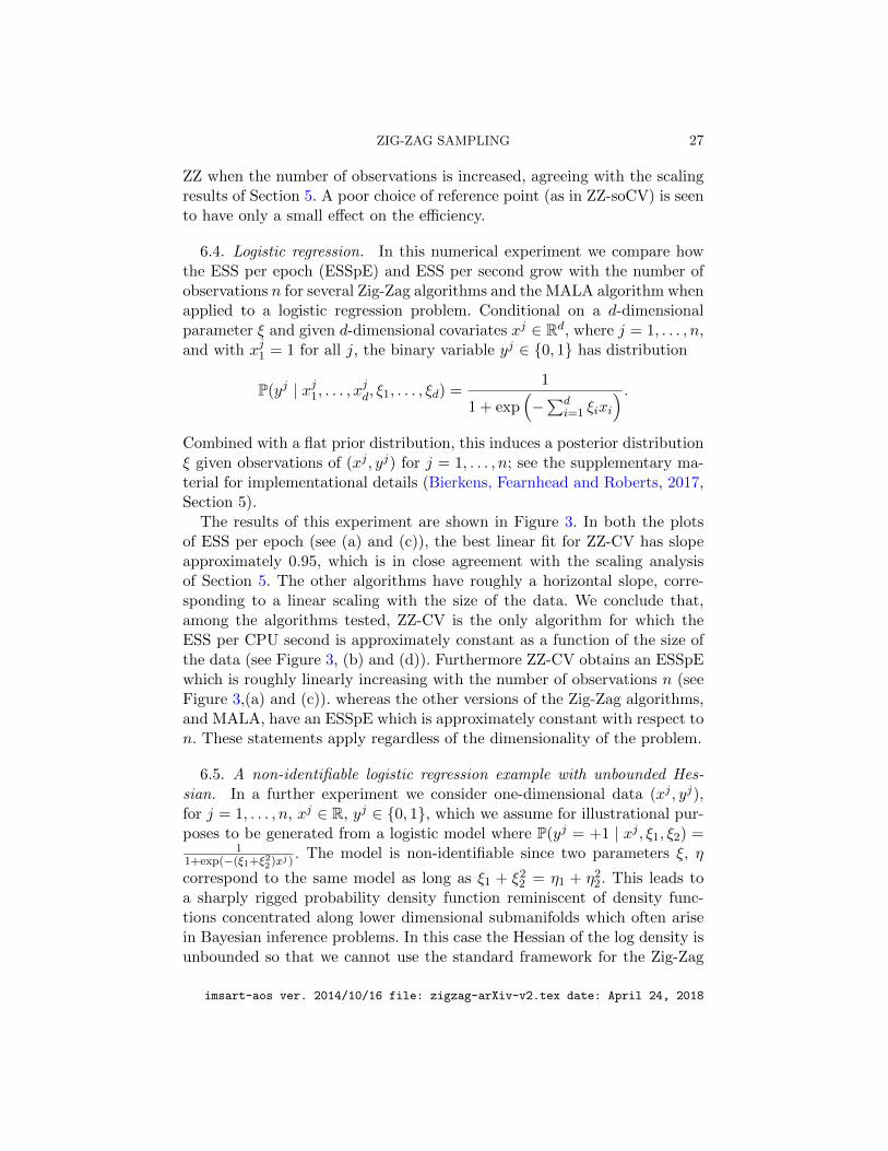
6.3. Mean of a Gaussian distribution. Consider the illustrative problemof estimating the mean of a Gaussian distribution. This problem has theadvantage that it allows for an analytical solution which can be comparedwith the numerical solutions obtained by Zig-Zag Sampling and other meth-ods. Conditional on a one-dimensional parameter ξ, the data is assumedto be i.i.d. from N(ξ, σ2). Furthermore a N(0, 1/ρ2) prior on ξ is specified.Data are generated from the true distribution N(ξ0, σ

2) for some fixed ξ0.For a detailed description of the experiment and computational bounds, seeSection 4 of the supplementary material.

In this experiment, we compare the mean square error (MSE) for severalalgorithms, namely basic Zig-Zag (ZZ), Zig-Zag with Control Variates (ZZ-CV), Zig-Zag with Control Variates with a “sub-optimal” reference point(ZZ-soCV), and Stochastic Gradient Langevin Dynamics (SGLD). SGLDis implemented with fixed step size, as is usually done in practice, see e.g.Vollmer, Zygalakis and Teh (2015), with the added benefit that it makesthe comparison with the Zig-Zag algorithms more straightforward. Here inbasic Zig-Zag we pretend that every iteration requires the evaluation of nobservations (whereas in practice, we can pre-compute ξMAP).

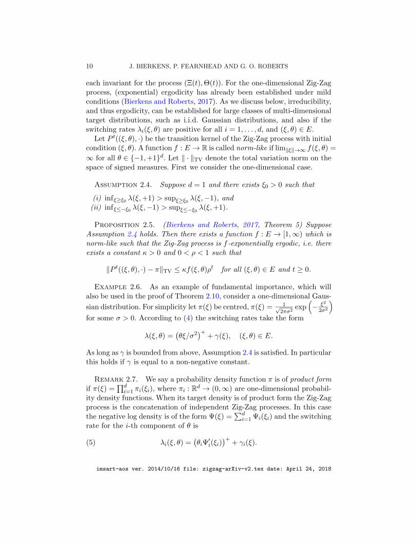
Results for this experiment are displayed in Figure 2. The MSE for thesecond moment using SGLD does not decrease beyond a fixed value, in-dicating the presence of bias in SGLD. This bias does not appear in thedifferent versions of Zig-Zag sampling, agreeing with the theoretical resultthat ergodic averages over Zig-Zag trajectories are consistent. Furthermorewe see a significant relative increase in efficiency for ZZ-(so)CV over basic


ZIG-ZAG SAMPLING 27

ZZ when the number of observations is increased, agreeing with the scalingresults of Section 5. A poor choice of reference point (as in ZZ-soCV) is seento have only a small effect on the efficiency.

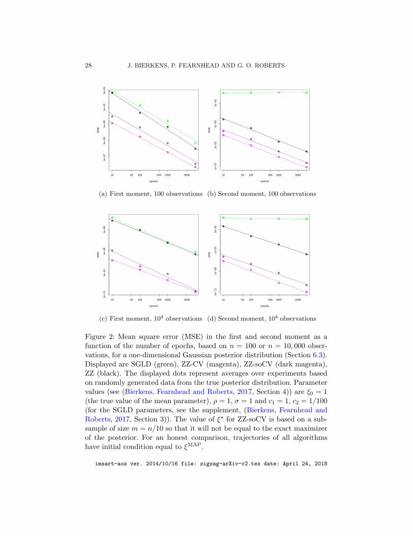
6.4. Logistic regression. In this numerical experiment we compare howthe ESS per epoch (ESSpE) and ESS per second grow with the number ofobservations n for several Zig-Zag algorithms and the MALA algorithm whenapplied to a logistic regression problem. Conditional on a d-dimensionalparameter ξ and given d-dimensional covariates xj ∈ Rd, where j = 1, . . . , n,and with xj1 = 1 for all j, the binary variable yj ∈ {0, 1} has distribution

P(yj | xj1, . . . , xjd, ξ1, . . . , ξd) =

1

1 + exp(−∑d

i=1 ξixi

) .Combined with a flat prior distribution, this induces a posterior distributionξ given observations of (xj , yj) for j = 1, . . . , n; see the supplementary ma-terial for implementational details (Bierkens, Fearnhead and Roberts, 2017,Section 5).

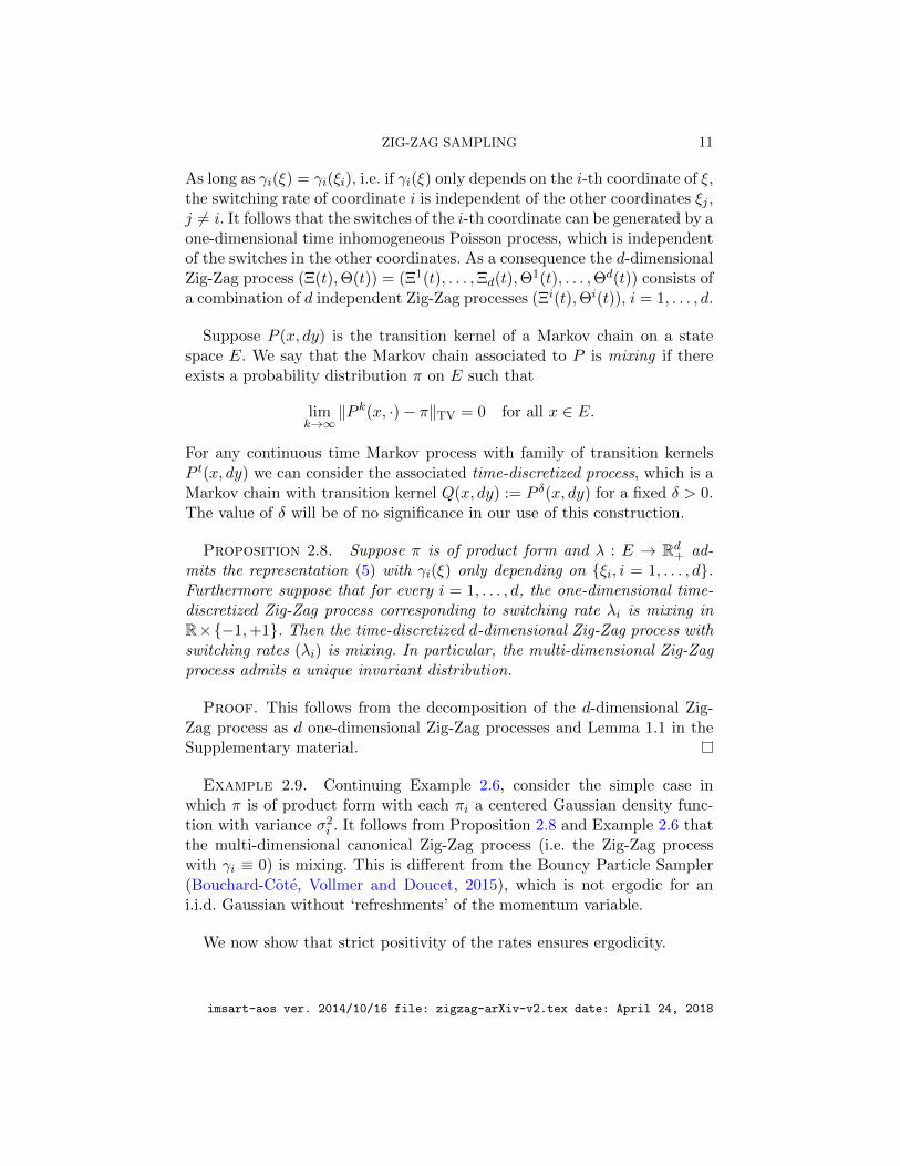
The results of this experiment are shown in Figure 3. In both the plotsof ESS per epoch (see (a) and (c)), the best linear fit for ZZ-CV has slopeapproximately 0.95, which is in close agreement with the scaling analysisof Section 5. The other algorithms have roughly a horizontal slope, corre-sponding to a linear scaling with the size of the data. We conclude that,among the algorithms tested, ZZ-CV is the only algorithm for which theESS per CPU second is approximately constant as a function of the size ofthe data (see Figure 3, (b) and (d)). Furthermore ZZ-CV obtains an ESSpEwhich is roughly linearly increasing with the number of observations n (seeFigure 3,(a) and (c)). whereas the other versions of the Zig-Zag algorithms,and MALA, have an ESSpE which is approximately constant with respect ton. These statements apply regardless of the dimensionality of the problem.

6.5. A non-identifiable logistic regression example with unbounded Hes-sian. In a further experiment we consider one-dimensional data (xj , yj),for j = 1, . . . , n, xj ∈ R, yj ∈ {0, 1}, which we assume for illustrational pur-poses to be generated from a logistic model where P(yj = +1 | xj , ξ1, ξ2) =

11+exp(−(ξ1+ξ2

2)xj). The model is non-identifiable since two parameters ξ, η

correspond to the same model as long as ξ1 + ξ22 = η1 + η2

2. This leads toa sharply rigged probability density function reminiscent of density func-tions concentrated along lower dimensional submanifolds which often arisein Bayesian inference problems. In this case the Hessian of the log density isunbounded so that we cannot use the standard framework for the Zig-Zag



●

●

●

●

10 50 100 500 1000 5000

1e−

071e

−06

1e−

051e

−04

1e−

03

epochs

MS

E

●

●

●

●

●

●

●

●

●

●

●

●

(a) First moment, 100 observations

● ● ● ●

10 50 100 500 1000 5000

1e−

071e

−05

1e−

031e

−01

epochs

MS

E

●

●

●

●

●

●

●

●

●

●

●

●

(b) Second moment, 100 observations

●

●

●

●

10 50 100 500 1000 5000

1e−

121e

−10

1e−

081e

−06

epochs

MS

E

●

●

●

●

●

●

●

●

●

●

●

●

(c) First moment, 104 observations

●● ● ●

10 50 100 500 1000 5000

1e−

111e

−09

1e−

071e

−05

epochs

MS

E

●

●

●

●

●

●

●

●

●

●

●

●

(d) Second moment, 104 observations

Figure 2: Mean square error (MSE) in the first and second moment as afunction of the number of epochs, based on n = 100 or n = 10, 000 obser-vations, for a one-dimensional Gaussian posterior distribution (Section 6.3).Displayed are SGLD (green), ZZ-CV (magenta), ZZ-soCV (dark magenta),ZZ (black). The displayed dots represent averages over experiments basedon randomly generated data from the true posterior distribution. Parametervalues (see (Bierkens, Fearnhead and Roberts, 2017, Section 4)) are ξ0 = 1(the true value of the mean parameter), ρ = 1, σ = 1 and c1 = 1, c2 = 1/100(for the SGLD parameters, see the supplement, (Bierkens, Fearnhead andRoberts, 2017, Section 3)). The value of ξ? for ZZ-soCV is based on a sub-sample of size m = n/10 so that it will not be equal to the exact maximizerof the posterior. For an honest comparison, trajectories of all algorithmshave initial condition equal to ξMAP.


ZIG-ZAG SAMPLING 29

● ●● ● ●

●

6 7 8 9 10 11

−6

−4

−2

02

4

● ● ● ● ● ●

● ● ● ●● ●

●

●

●

●

●

●

●● ●

●●

●

log(number of observations) base 2

log(

ES

S /

epoc

h) b

ase

2

(a) ESS per epoch, 2 dimensions

●

●

●

●

●

●

6 7 8 9 10 11

68

1012

1416

●

●

●

●

●

●

●

●

●

●

●

●

● ● ●●

●●

●

●

●

●

●

●


log(

ES

S p

er s

econ

d) b

ase

2

(b) ESS per second, 2 dimensions

●

● ●

● ●● ●

8 9 10 11 12 13

−9

−8

−7

−6

−5

−4

−3

−2

● ● ● ● ● ● ●

●

● ● ● ● ● ●

●

●

●

●

●

●

●

●

●

●

● ●

●●


log(

ES

S /

epoc

h) b

ase

2

(c) ESS per epoch, 16 dimensions

●●

●

●

●

●

●

8 9 10 11 12 13

02

46

810

●

●

●

●

●

●

●

●

●

●

●

●

●

●

●●

● ●●

●

●

●

●

●

●

●

●

●


log(

ES

S p

er s

econ

d) b

ase

2

(d) ESS per second, 16 dimensions

Figure 3: Log-log plots of the experimentally observed dependence of ESSper epoch (ESSpE) and ESS per second (ESSpS) with respect to the first co-ordinate Ξ1, as a function of the number of observations n in the case of (2-Dand 16-D) Bayesian logistic regression (Section 6.4). Data is randomly gen-erated based on true parameter values ξ0 = (1, 2) (2-D) and ξ0 = (1, . . . , 1)(16-D). Trajectories all start in the true parameter value ξ0. Plotted are meanand standard deviation over 10 experiments, along with the best linear fit.Displayed are MALA (tuned to have optimal acceptance ratio, green), Zig-Zag with global bound (red), Zig-Zag with Lipschitz bound (black), ZZ-SSusing global bound (blue) and ZZ-CV (magenta), all run for 105 epochs. Asreference point for ZZ-CV we compute the posterior mode numerically, thecost of which is negligible compared to the MCMC. The experiments arecarried out in R with C++ implementations of all algorithms.



algorithms. It is discussed in the supplementary material (Bierkens, Fearn-head and Roberts, 2017, Section 6), how to obtain computational bounds forthe Zig-Zag and ZZ-CV algorithms, which may serve as an illustration onhow to obtain such bounds in settings beyond those described in Sections 3.3and 4.3.

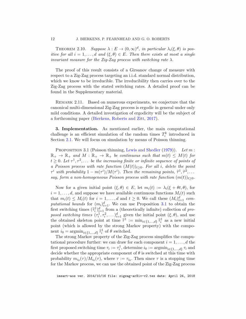
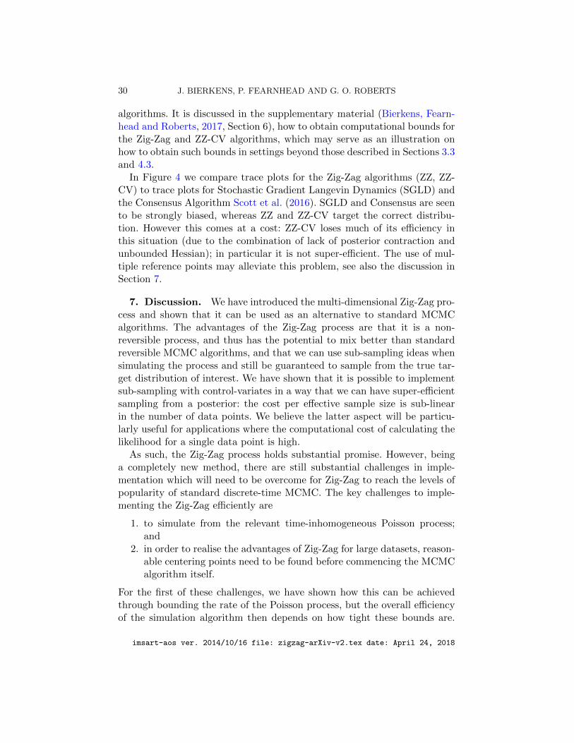
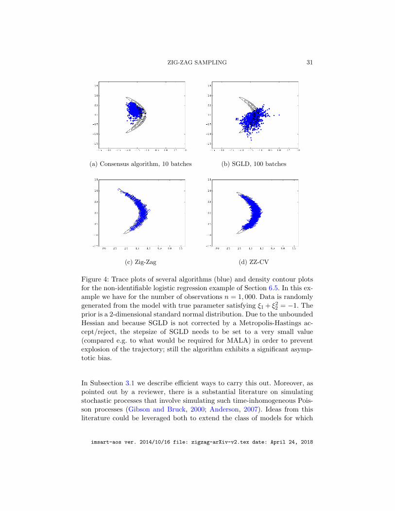
In Figure 4 we compare trace plots for the Zig-Zag algorithms (ZZ, ZZ-CV) to trace plots for Stochastic Gradient Langevin Dynamics (SGLD) andthe Consensus Algorithm Scott et al. (2016). SGLD and Consensus are seento be strongly biased, whereas ZZ and ZZ-CV target the correct distribu-tion. However this comes at a cost: ZZ-CV loses much of its efficiency inthis situation (due to the combination of lack of posterior contraction andunbounded Hessian); in particular it is not super-efficient. The use of mul-tiple reference points may alleviate this problem, see also the discussion inSection 7.

7. Discussion. We have introduced the multi-dimensional Zig-Zag pro-cess and shown that it can be used as an alternative to standard MCMCalgorithms. The advantages of the Zig-Zag process are that it is a non-reversible process, and thus has the potential to mix better than standardreversible MCMC algorithms, and that we can use sub-sampling ideas whensimulating the process and still be guaranteed to sample from the true tar-get distribution of interest. We have shown that it is possible to implementsub-sampling with control-variates in a way that we can have super-efficientsampling from a posterior: the cost per effective sample size is sub-linearin the number of data points. We believe the latter aspect will be particu-larly useful for applications where the computational cost of calculating thelikelihood for a single data point is high.

As such, the Zig-Zag process holds substantial promise. However, beinga completely new method, there are still substantial challenges in imple-mentation which will need to be overcome for Zig-Zag to reach the levels ofpopularity of standard discrete-time MCMC. The key challenges to imple-menting the Zig-Zag efficiently are

1. to simulate from the relevant time-inhomogeneous Poisson process;and

2. in order to realise the advantages of Zig-Zag for large datasets, reason-able centering points need to be found before commencing the MCMCalgorithm itself.

For the first of these challenges, we have shown how this can be achievedthrough bounding the rate of the Poisson process, but the overall efficiencyof the simulation algorithm then depends on how tight these bounds are.


ZIG-ZAG SAMPLING 31

(a) Consensus algorithm, 10 batches (b) SGLD, 100 batches

(c) Zig-Zag (d) ZZ-CV

Figure 4: Trace plots of several algorithms (blue) and density contour plotsfor the non-identifiable logistic regression example of Section 6.5. In this ex-ample we have for the number of observations n = 1, 000. Data is randomlygenerated from the model with true parameter satisfying ξ1 + ξ2

2 = −1. Theprior is a 2-dimensional standard normal distribution. Due to the unboundedHessian and because SGLD is not corrected by a Metropolis-Hastings ac-cept/reject, the stepsize of SGLD needs to be set to a very small value(compared e.g. to what would be required for MALA) in order to preventexplosion of the trajectory; still the algorithm exhibits a significant asymp-totic bias.

In Subsection 3.1 we describe efficient ways to carry this out. Moreover, aspointed out by a reviewer, there is a substantial literature on simulatingstochastic processes that involve simulating such time-inhomogeneous Pois-son processes (Gibson and Bruck, 2000; Anderson, 2007). Ideas from thisliterature could be leveraged both to extend the class of models for which



we can simulate the Zig-Zag process, and also to make implementation ofsimulation algorithms more efficient.

The second challenge applies when using the ZZ-CV algorithm to obtainsuper-efficiency for big data as discussed in Subsection 4.3. Although in ourexperience finding appropriate centering points is rarely a serious problem,it is difficult to give a prescriptive recipe for this step.

On the face of it, these challenges may limit the practical applicability ofZig-Zag, at least in the short term. With that in mind, we have released anR/Rcpp package for logistic regression, as well as the code which reproducesthe experiments of Section 6 (Bierkens, 2017).

In addition, while Zig-Zag is an exact approximate simulation method,there are various short-cuts to speed it up at the expense of the introductionof an approximation. For instance, there are already ideas of approximatelysimulating the continuous-time dynamics, through approximate bounds onthe Poisson rate (Pakman et al., 2016). These ideas can lead to efficientsimulation of the Zig-Zag process for a wide class of models, albeit with theloss of exactness. Understanding the errors introduced by such an approachis an open area.

The most exciting aspect of the Zig-Zag process is the super-efficiency weobserve when using sub-sampling with control variates. Already this idea hasbeen adapted and shown to apply to other recent continuous-time MCMCalgorithms (Fearnhead et al., 2018; Pakman et al., 2016). We have shownin Subsection 6.5 that Zig-Zag can be applied effectively within highly non-Gaussian examples where rival approximate methods such as SGLD and theConsensus Algorithm are seriously biased. So there is no intrinsic reason toexpect Zig-Zag to rely on the target distribution being close to Gaussian,although posterior contraction and the ability to find tight Poisson processrate bounds play important roles as we saw in our examples. There is muchto learn about how the efficiency of Zig-Zag depends on the statistical prop-erties of the posterior distribution. However, unlike its approximate com-petitors, Zig-Zag will still remain an exact approximate method whateverthe structure of the target distribution.

In truly ‘big data’ settings, in principle we still need to process all the dataonce, although a suitable reference point can be determined using a subset ofthe data, we do need to evaluate the full gradient of the log density once atthis reference point, and this computation is O(n). This operation howeveris much easier to parallelize than MCMC is, and after this approximatelyindependent samples can be obtained at a cost of O(1) each. Thus if wewish to obtain k approximately independent samples, the computationalefficiency of ZZ-CV is O(k + n) while the complexity of traditional MCMC


ZIG-ZAG SAMPLING 33

algorithms is O(kn). This is confirmed by the experiment in Section 6.4.The idea for control variates we present in this paper is just one, possibly

the simplest, implementation of this idea. There are natural extensions todeal with e.g. multi-modal posteriors or situations where we do not haveposterior concentration for all parameters. The simplest of these involveusing multiple reference points and monitoring the computational bound weget within the CV-ZZ algorithm and switching to a different algorithm whenwe stray so far from a reference point that this bound becomes too large.More sophisticated approaches include using the ideas from (Dubey et al.,2016), where we introduce a reference point for each data point and updatethe reference points for data within the subsample at each iteration of thealgorithm. This would lead to the estimate of the gradient that we centerour control variate estimator around to depend on the recent history of theZig-Zag process, and thus could be accurate even if we explore multiplemodes or the tails of the target distribution.

Acknowledgements. The authors are grateful for helpful comments fromreferees, the editor and the associate editor which have improved the paper.Furthermore the authors acknowledge Matthew Moores (University of War-wick) for helpful advice on implementing the Zig-Zag algorithms as an Rpackage using Rcpp. All authors acknowledge the support of EPSRC underthe ilike grant: EP/K014463/1.

SUPPLEMENTARY MATERIAL

Supplement: Supplement to “The Zig-Zag Process and Super-Efficient Sampling for Bayesian Analysis of Big Data”(doi: COMPLETED BY THE TYPESETTER; .pdf). Mathematics of theZig-Zag process, scaling of SGLD, details on the experiments including howto obtain computational bounds.

References.

Anderson, D. F. (2007). A modified next reaction method for simulating chemical sys-tems with time dependent propensities and delays. The Journal of Chemical Physics127 214107.

Andrieu, C. and Roberts, G. O. (2009). The pseudo-marginal approach for efficientMonte Carlo computations. The Annals of Statistics 37 697–725.

Bardenet, R., Doucet, A. and Holmes, C. (2015). On Markov Chain Monte CarloMethods for Tall Data. arXiv preprint arXiv:1505.02827.

Bierkens, J. (2015). Non-reversible Metropolis-Hastings. Statistics and Computing 251-16.

Bierkens, J. (2017). Computer experiments accompanying J. Bierkens, P. Fearnhead andG. Roberts, The Zig-Zag Process and Super-Efficient Sampling for Bayesian Analysis


http://dx.doi.org/COMPLETED BY THE TYPESETTER


of Big Data. https: // github. com/ jbierkens/ zigzag-experiments . Date accessed:20-10-2017.

Bierkens, J., Fearnhead, P. and Roberts, G. O. (2017). Supplement to “The Zig-ZagProcess and Super-Efficient Sampling for Bayesian Analysis of Big Data”.

Bierkens, J. and Roberts, G. (2017). A piecewise deterministic scaling limit of liftedMetropolis–Hastings in the Curie–Weiss model. Ann. Appl. Probab. 27 846–882.

Bierkens, J., Roberts, G. O. and Zitt, P.-A. (2017). Ergodicity of the zigzag process.arXiv preprint arXiv: 1712.09875.

Bouchard-Cote, A., Vollmer, S. J. and Doucet, A. (2015). The Bouncy Parti-cle Sampler: A Non-Reversible Rejection-Free Markov Chain Monte Carlo Method.arXiv:1510.02451.

Chen, T.-L. and Hwang, C.-R. (2013). Accelerating reversible Markov chains. Statistics& Probability Letters 83 1956–1962.

Deligiannidis, G., Bouchard-Cote, A. and Doucet, A. (2017). Exponential Ergod-icity of the Bouncy Particle Sampler. arXiv preprint arXiv: 1705.04579.

Duane, S., Kennedy, A. D., Pendleton, B. J. and Roweth, D. (1987). Hybrid MonteCarlo. Physics Letters B 195 216–222.

Dubey, K. A., Reddi, S. J., Williamson, S. A., Poczos, B., Smola, A. J. andXing, E. P. (2016). Variance reduction in stochastic gradient Langevin dynamics. InAdvances in Neural Information Processing Systems 1154–1162.

Duncan, A. B., Lelievre, T. and Pavliotis, G. A. (2016). Variance Reduction usingNonreversible Langevin Samplers. Journal of Statistical Physics 163 457–491.

Fearnhead, P., Bierkens, J., Pollock, M. and Roberts, G. O. (2018). PiecewiseDeterministic Markov Processes for Continuous-Time Monte Carlo. To appear in Sta-tistical Science.

Fontbona, J., Guerin, H. and Malrieu, F. (2012). Quantitative estimates for thelong-time behavior of an ergodic variant of the telegraph process. Advances in AppliedProbability 44 977–994.

Fontbona, J., Guerin, H. and Malrieu, F. (2016). Long time behavior of TelegraphProcesses under convex potentials. Stochastic Processes and their Applications. in press.

Gibson, M. A. and Bruck, J. (2000). Efficient exact stochastic simulation of chemicalsystems with many species and many channels. The Journal of Physical Chemistry A104 1876–1889.

Hastings, W. (1970). Monte Carlo sampling methods using Markov chains and theirapplications. Biometrika 57 97–109.

Hwang, C., Hwang-Ma, S. and Sheu, S. (1993). Accelerating Gaussian diffusions. TheAnnals of Applied Probability 3 897–913.

Jacob, P. E. and Thiery, A. H. (2015). On nonnegative unbiased estimators. The Annalsof Statistics 43 769–784.

Johnson, R. A. (1970). Asymptotic Expansions Associated with Posterior Distributions.Annals of Mathematical Statistics 41 851–864.

Lewis, P. A. W. and Shedler, G. S. (1979). Simulation of nonhomogeneous Poissonprocesses by thinning. Naval Res. Logist. Quart. 26 403–413.

Li, C., Srivastava, S. and Dunson, D. B. (2017). Simple, scalable and accurate posteriorinterval estimation. Biometrika 104 665–680.

Ma, Y.-A., Chen, T. and Fox, E. (2015). A complete recipe for stochastic gradientMCMC. In Advances in Neural Information Processing Systems 2917–2925.

Maclaurin, D. and Adams, R. P. (2014). Firefly Monte Carlo: Exact MCMC withSubsets of Data. In Proceedings of the 30th Conference on Uncertainty in ArtificialIntelligence. AUAI Press.


https://github.com/jbierkens/zigzag-experiments

ZIG-ZAG SAMPLING 35

Metropolis, N., Rosenbluth, A. W., Rosenbluth, M. N., Teller, A. H. andTeller, E. (1953). Equation of State Calculations by Fast Computing Machines. TheJournal of Chemical Physics 21 1087.

Monmarche, P. (2014). Hypocoercive relaxation to equilibrium for some kinetic modelsvia a third order differential inequality. arXiv:1306.4548.

Neal, R. M. (1998). Suppressing random walks in Markov chain Monte Carlo usingordered overrelaxation. In Learning in graphical models 205–228. Springer.

Neiswanger, W., Wang, C. and Xing, E. (2013). Asymptotically Exact, EmbarrassinglyParallel MCMC. arXiv:1311.4780.

Pakman, A., Gilboa, D., Carlson, D. and Paninski, L. (2016). Stochastic BouncyParticle Sampler. arXiv preprint arXiv:1609.00770.

Peters, E. A. J. F. and De With, G. (2012). Rejection-free Monte Carlo sampling forgeneral potentials. Physical Review E - Statistical, Nonlinear, and Soft Matter Physics85 1–5.

Pollock, M., Fearnhead, P., Johansen, A. M. and Roberts, G. O. (2016). The Scal-able Langevin Exact Algorithm: Bayesian Inference for Big Data. arXiv:1609.03436.

Quiroz, M., Villani, M. and Kohn, R. (2015). Speeding up MCMC by efficient datasubsampling. Riksbank Research Paper Series 121.

Rey-Bellet, L. and Spiliopoulos, K. (2015). Irreversible Langevin samplers and vari-ance reduction: a large deviations approach. Nonlinearity 28 2081–2103.

Roberts, G. O. and Tweedie, R. L. (1996). Exponential Convergence of LangevinDistributions and Their Discrete Approximations. Bernoulli 2 pp. 341–363.

Scott, S. L., Blocker, A. W., Bonassi, F. V., Chipman, H. A., George, E. I.and McCullogh, R. E. (2016). Bayes and Big Data: The Consensus Monte CarloAlgorithm. International Journal of Management Science and Engineering Management11 78-88.

Turitsyn, K. S., Chertkov, M. and Vucelja, M. (2011). Irreversible Monte Carloalgorithms for efficient sampling. Physica D: Nonlinear Phenomena 240 410–414.

Vollmer, S. J., Zygalakis, K. C. and Teh, Y. W. (2015). Exploration of the (Non-)asymptotic Bias and Variance of Stochastic Gradient Langevin Dynamics. arXivpreprint arXiv: 1501.00438.

Wang, X. and Dunson, D. B. (2013). Parallelizing MCMC via Weierstrass Sampler.arXiv:1312.4605.

Welling, M. and Teh, Y. W. (2011). Bayesian learning via stochastic gradient Langevindynamics. In Proceedings of the 28th International Conference on Machine Learning(ICML-11) 681–688.

Delft Institute of Applied Mathematics,Van Mourik Broekmanweg 6,2628 XE Delft,Netherlands,E-mail: [email protected]

Department of Mathematics and Statistics,Fylde College,Lancaster University,Lancaster, LA1 4YF,United Kingdom,E-mail: [email protected]

Department of Statistics,University of Warwick,Coventry CV4 7AL,United Kingdom,E-mail: [email protected]


mailto:[email protected]



Documents

, Paul Fearnhead and Gareth Roberts … · The Zig-Zag Process and Super-E cient Sampling for Bayesian Analysis of Big Data Joris Bierkens 1, Paul Fearnhead 2 and Gareth Roberts 1