Embed Size (px)
Citation preview

-Omics and Imaging
Aad van der Lugt Department of Radiology
Erasmus MC, Rotterdam, the Netherlands

Summary
Imaging in biobanking
Consider imaging phenotypes as (surrogate) endpoint
Quantification of imaging biomarkers
Standardisation in acquisition and analysis
Big data approach
Link with -omics possible
Join and support BBMRI2.0

Topics
Population Studies
Role of Imaging
Image analysis
BBMRI 2.0
WP3 Imaging
WP2-WP3 -Omics versus Imaging
Examples
Atherosclerosis (Calcifications)
White matter lesions (WML)
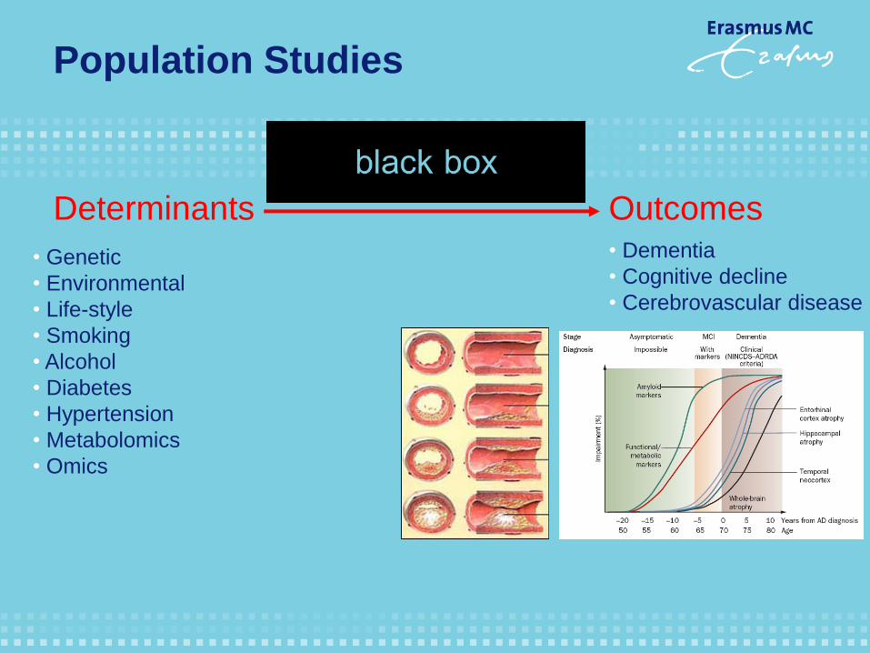
Population Studies
Determinants Outcomes
• Genetic
• Environmental
• Life-style
• Smoking
• Alcohol
• Diabetes
• Hypertension
• Metabolomics
• Omics
• Dementia
• Cognitive decline
• Cerebrovascular disease
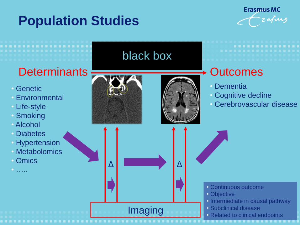
Determinants Outcomes
• Genetic
• Environmental
• Life-style
• Smoking
• Alcohol
• Diabetes
• Hypertension
• Metabolomics
• Omics
• …..
• Dementia
• Cognitive decline
• Cerebrovascular disease
Imaging
black box
Δ Δ
• Continuous outcome
• Objective
• Intermediate in causal pathway
• Subclinical disease
• Related to clinical endpoints
Population Studies

De Weert, AJNR 2009 /
Bos, Stroke 2012
Image analysis: Quantification of ICAC

1995: visual 2004: automated
Image analysis: White Matter Lesions
1999: manual

Image Analysis: Advanced Processing Tools
Volume and shape analysis
Courtesy Renske de Boer Courtesy Hakim Achterberg
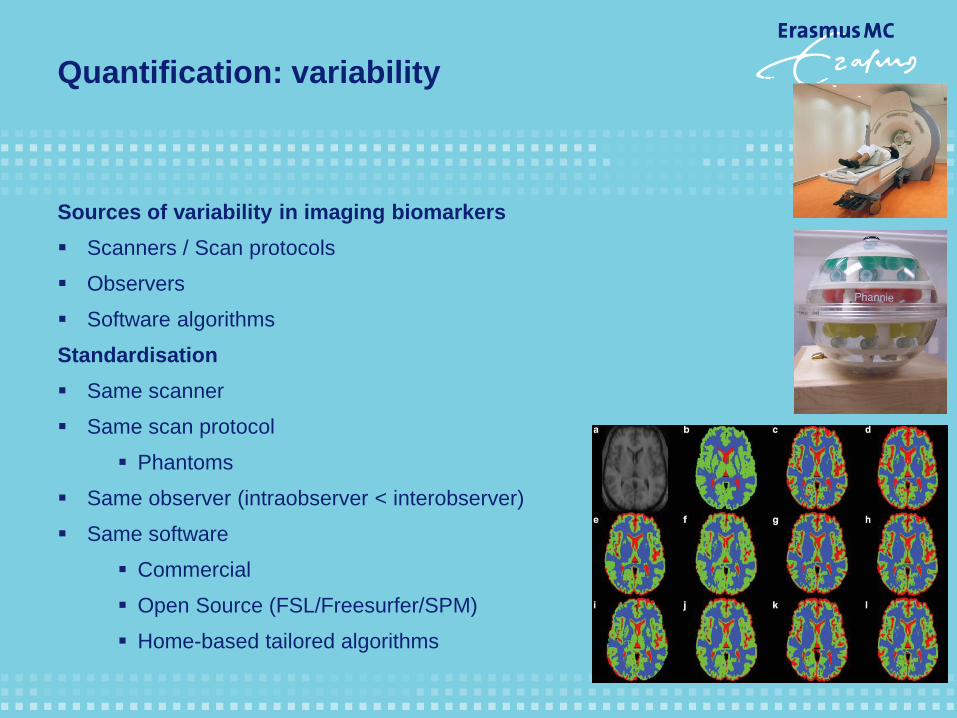
Quantification: variability
Sources of variability in imaging biomarkers
Scanners / Scan protocols
Observers
Software algorithms
Standardisation
Same scanner
Same scan protocol
Phantoms
Same observer (intraobserver < interobserver)
Same software
Commercial
Open Source (FSL/Freesurfer/SPM)
Home-based tailored algorithms

Deliverables BBMRi-WP3
Updated catalaque of cohorts with imaging
Image Data Storage
XNAT
User meetings
Make image analysis software sustainable / pipelines
Library of scan-rescan data (performance metrics)
Library of annotated data (training)
Access to image analysis pipelines in neuroimaging
Use cases
Reference database of imaging parameters
PSI - ND
Link with metabolomics WP2

Data-archive infrastructure / seamless connection to cloud/hp computing
XNAT anonymised DICOM images,
processed images, and annotations
OpenClinica other study
data
Image Processing Unit (FastR, ?)
Workflow based approach; standardization; data provenance (harmonization /ontology)
by the Euclidean path length L yields a mean measure over the
minimum cost path,gΓ:
gΓ≜1
L∫
L0g Γ sðÞ; Γ′ sðÞ ds: ð3Þ
The local measure can either be dependent or independent of
direction. It is therefore possible to use Eq. (3) to average the
(direction-independent) measuresFAandMDover theminimumcost
path. Both these measures are, however, based on the tensor model,
which has shortcomings as discussed before. We prefer a measure
that isnot based on a tensor model and use in thisproof of principle
study g x;vð Þ= ψ x;vð Þ. Our connectivity measure is themean cost uΓwhich equals:
uΓ =1
L∫
L0ψ Γ sðÞ; Γ′ sðÞ ds=
u R;pð Þ
L: ð4Þ
The local cost function depends on both local anisotropy and
diffusivity and itsaverage over the minimum cost path is therefore a
suitableconnectivity measure.Wechosetonormalizeby thelength of
theminimum cost path in order to correct for differencesin head size
and/or brain atrophy. Fig. 2 shows, for three example slices, the
cumulative costs, path length, and average costs over the minimum
cost pathsstarting in the right amygdala.
Construction of the mcp-network
To enable statistical analysis of mcp-networks, corresponding
brain regions should be defined in all subjects. We use the publicly
availableFreeSurfer softwarepackage, which iscapableof segment-
ing subcortical structures (Fischl et al., 2004b) and parcellating the
cortex (Fischl et al., 2004a) based on T1-weighted (T1w) images.
The T1w scan is rigidly registered to the b0 diffusion image using
Elastix (Klein et al., 2010). The FreeSurfer segmentation and
parcellation aretransformed toDWI spaceaccordingto theresulting
transformation. The gray and white matter mask, used to restrict the
Fast Sweeping algorithm to the brain, is defined by the FreeSurfer
segmentation.
Additionally, the FreeSurfer segmentation of the subcortical
structuresand cortical parcellation definethestart and target regions.
In thispaper, weusetheterm connection to refer to an mcp-network
connectionbetweentwonodes,or (thetrajectoryof) thecorresponding
minimum cost path. This does not necessarily correspond to a direct
anatomical connection between thetwobrain regions.Moreover, in an
anatomical connection theminimumcost path runsfromstart region to
target region,which isnot necessarily thesamedirection assignalsare
transported alongthewhitematter path.
An mcp-network consistsof nconnectionsthat areweighted by uΓ.
Asevery voxel in the target region hasadifferent uΓ,onevalue needs
tobedefined torepresent theconnection between thestart and target
region.Weusethevalueof uΓ of thevoxel with minimum cumulative
cost uðR;pÞ. All the minimum cost paths running to the target region
most probably run through the same white matter bundle. Of these
paths, the minimum cost path running to the voxel with minimum
cumulative cost is the most optimal.
Using the uΓ at the representing voxels, mcp-networks are
obtained for themsubjects. All of thesemcp-networksarecombined
into an m×n matrix of connectivity features for statistical analysis.
Statistical analysis
SAMSCo usesstatistical analysisto investigatewhether thematrix
of connectivity features contains information regarding connectivity
changese.g.dueto normal agingor neurodegenerativedisease.Based
on this matrix, we investigated the prediction of variables such as
subject age using regression, and the classification of subjects into
groups defined by markers of brain tissue degeneration.
Regression
Multivariateregression can beused topredict aparticular variable
y, e.g. a disease severity index or subject age, based on the matrix of
connectivity features. In linear regression, the predicted value y de-
pendson the vector of input variables f = f1; f2; :::; fNð ÞT:
y = ∑N
j = 1
fjβj + β0; ð5Þ
with βj the regression coefficients, and β0 the intercept. When the
matrix of connectivity featuresisused asregression input, thelength of
Fig. 1.Schematicoverview of theSAMSCo framework for statistical group analysisof structural brain connectivity.Connectivity isestablished through minimum cost paths(mcp's)
that areconstructed usingdiffusion weighted images. Themcp'srun from start to target regionsdefined by FreeSurfer segmentation and cortical parcellation. Theimageshowsthe
mcp'sstarting at the left putamen and aslice of thecorresponding cumulative cost image. Per subject an mcp-network isconstructed based on themcp'sand thecumulative cost
over, and path length of, these mcp's. The mcp-networksof all m subjects are combined into amatrix of connectivity features for statistical analysis.
559R. de Boer et al. / NeuroImage 55 (2011) 557–565
prediction of disease development in an asymptomatic
population, as differences between subjects in the latter
group are much more subtle. In our study, all persons
were nondemented at scan time and developed dementia
only later. Therefore, our results support the use of shape
as a predictive marker.
The most notable other imaging methods used for
extracting features for dementia classification are based on
voxel-based morphometry (VBM) [e.g., Fan et al., 2007;
Kl€oppel et al., 2008] and cortical thickness [e.g., Desikan
et al., 2009; Querbes et al., 2009]. Cuingnet et al. [2010]
compared these methods of dementia classification, using
a large dataset from the AD Neuroimaging Initiative data-
base. They compared three groups of methods: VBM, cort-
ical thickness measurements and hippocampus volume/
shape based methods. They found that for AD versus con-
trol classification the whole brain methods outperformed
the hippocampus-based methods. However, for MCI-c ver-
sus control classification the hippocampal methods were
competitive with the whole-brain methods. This result
confirms that the hippocampus is one of the regions in the
brain where atrophy is noticeable first in subjects with
dementia.
We are not aware of any work using pattern recognition
techniques to evaluate predictive value of hippocampal
shape on similar data used in our study. There are studies
which use statistical methods (e.g., regression or analysis
of variance) to evaluate predictive value. Csernansky et al.
[2005] and Apostolova et al. [2010] studied hippocampal
shape using comparable subject groups. Their studies
were more descriptive of nature making it impossible to
quantitatively compare their results to our study. We can,
however, qualitatively compare the discriminative direc-
tion obtained in our study to the maps obtained by
Csernansky et al. [2005, Fig. 3] and Apostolova et al. [2010,
Fig. 1]. For the left hippocampus, the discriminative direc-
tion maps presented in Figure 7 appears to match the atro-
phy and significance maps presented by Csernansky and
Apostolova respectively: most influential points are found
in the CA1 and Subiculum subfields. Csernansky also pro-
vides the direction of change, which corresponds with our
results. For the right hippocampus, the similarity between
the studies is lower: there are areas which contribute to
our classification in the CA2 subfield that Csernansky or
Apostolova do not find. This may be partly due to the fact
that the discriminative direction in our work is based on
the classifier that uses all points jointly, rather than the
group differences per point as used by Csernasky and
Apostolova. Also, Figure 6 shows asymmetry in the classi-
fication performance of the left and right hippocampus,
indicating that the right hippocampus might not contrib-
ute much discriminative information to the classifier.
Many studies have shown asymmetry in hippocampal
volume [Karas et al., 2004; Morra et al., 2009b; Scher et al.,
2011], atrophy rates [Morra et al., 2009a; Zhou et al., 2009],
or report differences in the diagnostic value of the left and
right hippocampus [Csernansky et al., 2005; Tepest et al.,
2008]. However, the asymmetry and the direction of asym-
metry are not consistent across studies. It has been sug-
gested that the asymmetry depends on the stage of
dementia; theleft hippocampus isaffected first by dementia
related atrophy and the right hippocampus follows with a
time lag [Morra et al., 2009b; Thompson et al., 2003, 2004;
Zhou et al., 2009]. In our data, the left hippocampus was
found to be more predictive for dementia, which fits the
suggested pattern for asymmetry; in our subjects, the dis-
ease is in a very early stage, and it is possible that the left
hippocampus is already affected, while the right
Figure 7.
The discriminative direction of the classifier. The colors represent coefficients of the classifier
localized on the hippocampal surface. The posterior probability of developing dementia increases
if the points move in the direction indicated by the colors: blue points further inward and red/
yellow points further outward indicate ahigher chance of developingdementia. [Color figure can
be viewed in the online issue, which isavailable at wileyonlinelibrary.com.]
r Achterberg et al. r
r 10 r
prediction of disease development in an asymptomatic
population, as differences between subjects in the latter
group are much more subtle. In our study, all persons
were nondemented at scan time and developed dementia
only later. Therefore, our results support the use of shape
as a predictive marker.
The most notable other imaging methods used for
extracting features for dementia classification are based on
voxel-based morphometry (VBM) [e.g., Fan et al., 2007;
Kl€oppel et al., 2008] and cortical thickness [e.g., Desikan
et al., 2009; Querbes et al., 2009]. Cuingnet et al. [2010]
compared these methods of dementia classification, using
a large dataset from the AD Neuroimaging Initiative data-
base. They compared three groups of methods: VBM, cort-
ical thickness measurements and hippocampus volume/
shape based methods. They found that for AD versus con-
trol classification the whole brain methods outperformed
the hippocampus-based methods. However, for MCI-c ver-
sus control classification the hippocampal methods were
competitive with the whole-brain methods. This result
confirms that the hippocampus is one of the regions in the
brain where atrophy is noticeable first in subjects with
dementia.
We are not aware of any work using pattern recognition
techniques to evaluate predictive value of hippocampal
shape on similar data used in our study. There are studies
which use statistical methods (e.g., regression or analysis
of variance) to evaluate predictive value. Csernansky et al.
[2005] and Apostolova et al. [2010] studied hippocampal
shape using comparable subject groups. Their studies
were more descriptive of nature making it impossible to
quantitatively compare their results to our study. We can,
however, qualitatively compare the discriminative direc-
tion obtained in our study to the maps obtained by
Csernansky et al. [2005, Fig. 3] and Apostolova et al. [2010,
Fig. 1]. For the left hippocampus, the discriminative direc-
tion maps presented in Figure 7 appears to match the atro-
phy and significance maps presented by Csernansky and
Apostolova respectively: most influential points are found
in the CA1 and Subiculum subfields. Csernansky also pro-
vides the direction of change, which corresponds with our
results. For the right hippocampus, the similarity between
the studies is lower: there are areas which contribute to
our classification in the CA2 subfield that Csernansky or
Apostolova do not find. This may be partly due to the fact
that the discriminative direction in our work is based on
the classifier that uses all points jointly, rather than the
group differences per point as used by Csernasky and
Apostolova. Also, Figure 6 shows asymmetry in the classi-
fication performance of the left and right hippocampus,
indicating that the right hippocampus might not contrib-
ute much discriminative information to theclassifier.
Many studies have shown asymmetry in hippocampal
volume [Karas et al., 2004; Morra et al., 2009b; Scher et al.,
2011], atrophy rates [Morra et al., 2009a; Zhou et al., 2009],
or report differences in the diagnostic value of the left and
right hippocampus [Csernansky et al., 2005; Tepest et al.,
2008]. However, the asymmetry and the direction of asym-
metry are not consistent across studies. It has been sug-
gested that the asymmetry depends on the stage of
dementia; theleft hippocampus isaffected first by dementia
related atrophy and the right hippocampus follows with a
time lag [Morra et al., 2009b; Thompson et al., 2003, 2004;
Zhou et al., 2009]. In our data, the left hippocampus was
found to be more predictive for dementia, which fits the
suggested pattern for asymmetry; in our subjects, the dis-
ease is in a very early stage, and it is possible that the left
hippocampus is already affected, while the right
Figure 7.
The discriminative direction of the classifier. The colors represent coefficients of the classifier
localized on the hippocampal surface. The posterior probability of developingdementia increases
if the points move in the direction indicated by the colors: blue points further inward and red/
yellow points further outward indicate ahigher chance of developingdementia. [Color figure can
beviewed in the online issue, which isavailable at wileyonlinelibrary.com.]
r Achterberg et al. r
r 10 r
Data
The imaging data used in this study was a subset taken
from the Rotterdam Scan Study: a prospective, population-
based MRI study on age-related neurological diseases [den
Heijer et al., 2003; Ikram, 2011]. For 511 nondemented, el-
derly subjects, MRI scans and the age, gender, dementia
diagnosis, and time of follow-up were available.
All subjects were scanned in 1995–1996 on a Siemens
1.5T scanner. The sequence used was a custom designed,
inversion recovery, three-dimensional (3D) half-Fourier ac-
quisition single-shot turbo spin echo sequence. This
sequence had the following characteristics: inversion time
4,400 ms, repetition time 2,800 ms, effective echo time 29
ms, matrix size 192 3 256, flip angle 180 , slice thickness
1.25 mm, acquired in sagittal direction. The images were
reconstructed to a 128 3 256 3 256 matrix with a voxel
dimension of 1.25 3 1.0 3 1.0 mm.
Study participantswerefollowed during a10-year period.
During thisperiod, they were invited for four cognitive fol-
low-up tests, and the general practitioners records were
tracked for diagnosis of dementia. Dementia screening fol-
lowed astrict two-step protocol [den Heijer et al., 2006]; ini-
tially, participants were cognitively screened with the Mini
Mental StateExamination (MMSE) and theGeriatric Mental
Schedule. If the results of this initial screening indicated
possible dementia, a more thorough cognitive testing was
performed for verification. During thestudy period, 52per-
sons were diagnosed with dementia. The median interval
between MRI acquisition and dementia diagnosis was 4.0
yearswith an interquartile rangeof 4.8years.
The entire dataset, hereafter referred to as the cohort set,
contained 52 prodromal dementia cases and 459 persons
who did not develop dementia. To train and test a model
independent of age and gender, an age- and gender-
matched subset of 50 prodromal dementia subjects and
150 controls was identified, hereafter referred to as the
matched set. Characteristics of the cohort set and matched
set can be found in Table I. None of the subjects were
demented at the time the MRI scan was taken.
Because memory impairment is the first detectable neu-
ropsychological sign of incipient dementia, we questioned
persons on subjective memory complaints. This was done
by a single question: “Do you have complaints about your
memory performance?” Furthermore, objective memory
performance was assessed using a 15-word verbal learning
task [den Heijer et al., 2006] resulting in a memory score.
To increase the sample size in the matched set, we
selected three unique controls per case; this was possible
for 50 cases. The matching was performed using the fol-
lowing criteria: the gender had to be the same, the follow-
up time of the controls should be at least as long as the
time to diagnosis of the corresponding case, and the age
could not differ more than 1.5 years. To avoid significant
age differences, the mean age of the controls was kept as
close as possible to the age of the case. We verified that
the age matching resulted in no significant difference
between groups with a paired t-test.
Figure 1.
Overview of methods used: (1) MRI scans of the brain were
acquired. (2) In each scan, the left and right hippocampus was seg-
mented. (3) Thesegmentationswerepostprocessed. (4) Pointswere
distributed over each surface, such that points on a different scans
correspond with each other, and were concatenated to create one
feature vector per scan. (5) The dimensionality of the feature
vectors was reduced usingprincipal component analysis. (6) A Sup-
port Vector Machine classifier was used to predict dementia devel-
opment for each scan. Step (5) and (6) were performed in across-
validation manner (for a colored delineation in the figure, refer to
the web version of this article.) [Color figure can be viewed in the
online issue, which isavailableat wileyonlinelibrary.com.]
r Hippocampal Shape is Predictive for Dementia r
r 3 r
Transmart / Molgenis / ?
facilitating correlative analyses

Outcomes Determinants
Genetic Dementia
Stroke
• White matter lesions
...
-Omics and Imaging
CHARGE
RSS
FHS
CHS
AGES
ARIC
ASPS
n > 9000
Fornage M et al. Ann Neurol. 2011;69:928-39

Fornage et al. Annals of Neurology 2011
Ikram et al. Nature Genetics 2012
Bis et al. Nature Genetics 2011
O’Donnell et al. Circulation 2011
GWAS
Bis et al. Nature Genetics 2011 Debette et al.
Stroke 2010
Stein et al. Neuroimage 2010

Correlations between calcifications
Bos et al, Arterioscler Thromb Vasc Biol, 2011
Intracranial carotid artery calcification
Coronary artery
calcification
Aortic arch
calcification
Extracranial carotid artery
calcification
0.47 0.50 0.51

Vascular disease and stroke
Bos et al, JAMA Neurol 2014

Genetic susceptibility of ICAC
Adams et al, Stroke 2016
• Heritability (h2): 47 % (SE: 19%, P=0.009)
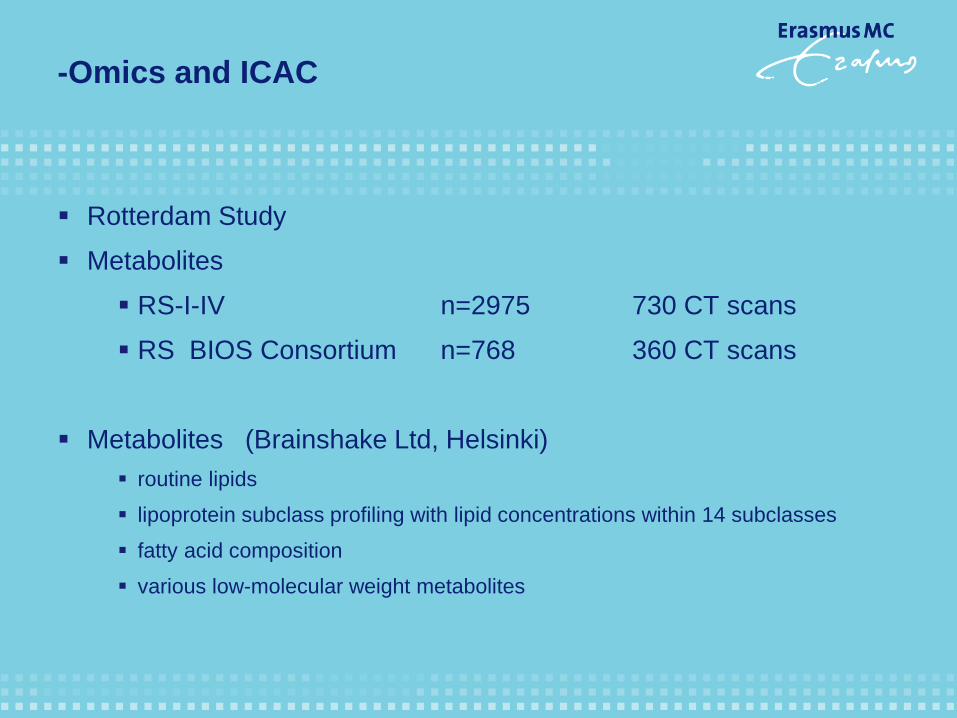
-Omics and ICAC
Rotterdam Study
Metabolites
RS-I-IV n=2975 730 CT scans
RS BIOS Consortium n=768 360 CT scans
Metabolites (Brainshake Ltd, Helsinki)
routine lipids
lipoprotein subclass profiling with lipid concentrations within 14 subclasses
fatty acid composition
various low-molecular weight metabolites

CT-based calcification

Methods
Metabolites: natural logarithmic or rank transformations
Calcifications: volumes mm3
Linear regression
Model 1 adjusting for age, gender, and lipid-lowering medication
Model 2 + hypertension, diabetes, hypercholesterolemia, BMI, and smoking
Model 3 + history of cardiovascular disease
2 datasets were meta-analysed
Correction for multiple testing

Results (1)
Polymers, which reside in Lp(a) (atherogenic effects)
Impaired glucose tolerance
Common genetic background

Results (2)

-Omics and WML
Brainshake and Brain MRI
The Maastricht Study (DMS)
Leiden Longevity Study (LLS)
Leiden University Migraine Neuro Analysis study (LUMINA)
Prospective Study of Pravastatin in the Elderly at Risk (PROSPER)
The Netherlands Study of Depression and Anxiety (NESDA)
Netherlands Twin Register (NTR)
Free University Medical Center Amsterdam Dementia Cohort (VUMC ADC)
Erasmus Rucphen Family (ERF) study
The Rotterdam Study (RS)
Metabolomics Imaging (Brain MRI) Working Group

Summary
Imaging in biobanking
Consider imaging phenotypes as (surrogate) endpoint
Quantification of imaging biomarkers
Standardisation in acquisition and analysis
Big data approach
Link with -omics possible
Join and support BBMRI2.0


Dept. of Epidemiology
Cock Van Duin
M. Arfan Ikram
Oscar Franco
Maryam Kavousi
Maarten Leening
Dept. of Radiology
Gabriel Krestin
Daniel Bos
Meike Vernooij
Wiro Niessen
Marius de Groot
Marcel Koek
Annegreet van Opbroek
Henri Vrooman
Specific collaborations on ICAC


Overlap BBMRI-NL / EPI2
Large scale analysis
Cataloque
Enrichment of existing data
Harmonisation data acquisition and analysis
Standardisation data acquisition and overlap
Open Access
IT - infrastructure
Integration with - omics

Image Data Storage Image Analysis Pipelines
• Brain tissue
• White matter lesions
• DTI: global measures and tractography
• Resting-state fMRI
Libraries • Standardized image acquisition protocols • Scan-rescan image data (for validation) • Annotated image data (atlasses) • Image datasets from cohort studies • Reference database of biomarkers
The infrastructure provides: advice on standardized image acquisition protocols, central imaging data storage facility including options for data viewing, validated image-analyses pipelines, multiple libraries for development and testing purposes by users of
the infrastructure, and normative reference databases generated for the various biomarkers which may serve as basis for scientific research or for clinical reference.
WP3 Image Analysis Infrastructure

The Rotterdam Study
Extensive data collection,
including:
- Interview
- Physical examinations
- Blood sampling
- Cognitive assessments
- Surveillance for major
diseases

The Rotterdam Study
Hofman, Eur J Epid, 2015

Susceptibility weighted
sequence Conventional T2* weighted
sequence
Detection of Cerebral Microbleeds

Imaging in BBMRI-NL2.0 Data
Data-acquisition
Data-analysis Pipelines
Catalogue (MIABIS 2.0)
Storage (XNAT- server)(user
meeting)
Collaboration - Pooling Image
Data
Open Access
Incidental Findings
Harmonisation
Standardisation
Harmonisation
Standardisation
Atlas / Annotated data
Inter- and intrascan image data
Grid computing
Open access

Problems in Imaging Biobanking
Storage (PACS / XNAT-server)
Raw data / Reconstructed data
Data analysis
Qualitative / Quantititive
Manual / Automated
Validation of quantitative biomarkers
Reproducibility
Within study (quality control - upgrades)
Between studies (scanner and protocol differences)
Extracted image biomarkers vs voxel based analysis
Machine learning