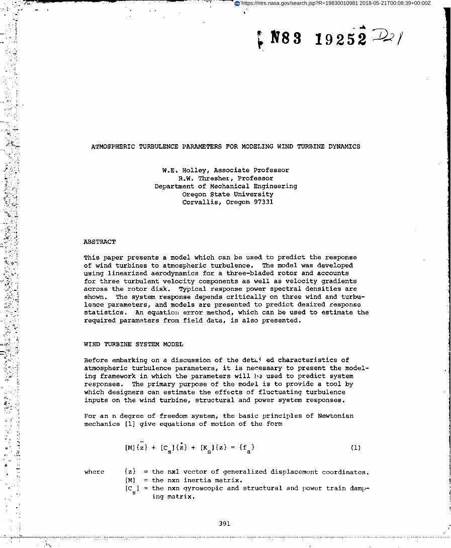
.,. ' . &'

" N83 19252,; '(,

__ o': I

fqi'• :,. :,, %,

fi_':£ ATMOSPHERIC TURBULENCE PARAMETERS FOR MODELING WIND TURBINE DYNAMICS

':"_" W.E Holley, Associate Professor

_"_'_, : R.W. Threshez, Professor

_4',,_':' Department of Mechanical Engineering

o,. _, Oregon State University

_¢_,, Corvallis, Oregon 97331

%:';:i:

--_i...)::i:,. ABSTRACT

_-::, This paper presents a model which can be used to predict the response

_..: of wind turbines to atmospheric turbulence. The model was developed

_jo-: using linearized aerodynamics for a three-bladed rotor and accounts

-_:(_ 'i for three turbulent velocity components as well as velocity gradientsacross the rotor disk. Typical response power spectral densities are

_:_)_-{ shown The system response depends critically on three wind and turbu-,:_'._'_";.__:'_. , lence parameters, and models are presented to predict desired zesponse

--'I)_.-_L_ statistics. An equation error method, which can be used to estimate the

-ii .-:.::::: required parameters from field data, is also presented.

=_o::'_: WIND TURBINE SYSTEM MODEL

_: . Before embarking on a discussion of the detaJ ed characteristics of

-:_":.':'i: atmospheric turbulence parameters, it is necessary to present the model-

,,!.¢:::: ing framework in which the parameters will b._ used to predict systemo_

•' i_ responses. The primary purpose of the model is to provide a tool by

which designers can estimate the eff¢:cts of fluctuating turbulence

_,,_ ,i inputs on the wind turbine, structural and power system responses.

•:_' For an n degree of freedom system, the basic principles of Newtonian

,; mechanics [i] give equations of motion of the form

'( :i:0 .!

{z}+ [cs]{_}+ [Ks]{z}= {f }[M] (I)

'; where {z} = the nxl vector of generalized displacement coordinates

', [M] = the nxn inertia matrix.

"_" : [Cs] = the nxn gyroscopic and structural and power train damp-, _ ing matrix.

https://ntrs.nasa.gov/search.jsp?R=19830010981 2018-05-21T00:08:39+00:00Z

&

ORIGINALPAGEIS_' OF pOORQUALITY. - f

[K ] _ the nxn structural and power train stiffness matrix.

{fs} = the nxl vector of aerodynamic forces and moments gener-

:. _ ated by the turbine rotoz.

The aerodynamic forcing term of Eq. (i) depends upon the motion of the

'_ turbine rotor with respect to the ground as well as the motion of the

air. If the aerodynamic forces and moments are linearized about a

_?_ steady operating condition, the following equation results

5

{fa } = {fn } + [F]{u} - [Ca]{z} - [Ka]{z} (2)

_: where {fn } = the nxl vector of steady, nominal aerodynamic forces:_ and moments. I

i {u} = the mxl vector of fluctuating turbulence inputs

i:_. [F] = the nxmmatrix of aerodynamic influence coefficients.

i- [C=] = the nxn aerodynamic damping matrix.

[K;] = the nxn aerodynamic stiffness matrix.! ;

i '_" In this particular model, the turbulence input vector {u} consists of

_ three velocity components which are uniform over the turbine rotor disk

: '_ and six additional gradient terms which account for variations in tur-

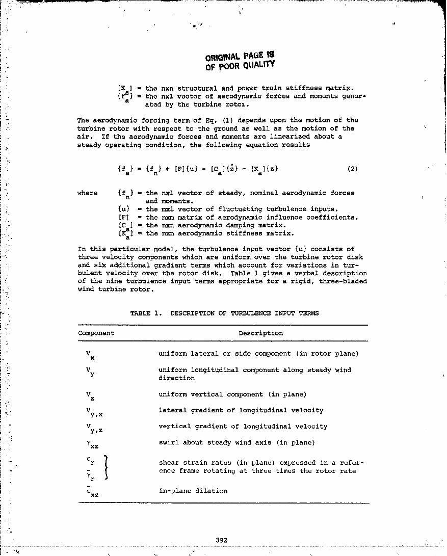
bulent velocity over the rotor disk. Table i gives a verbal description

of the nine turbulence input terms appropriate for a rigid, three-bladed

_._ wind turbine rotor.

i:__ TABLE i. DESCRIPTION OF TURBULENCE INPUT TERMS

: Component Description

V uniform lateral or side component (in rotor plane)x

i _:'_ V uniform longitudinal component along steady windi_- y_._ direction

V uniform vertical component (in plane)• z

_i.' V lateral gradient of longitudinal velocityy,x

" V vertical gradient of longitudinal velocity.,' y,z

. 7X z swirl about steady wind axis (in plane)

"_ er shear strain rates (in plane) expressed in a refer-

- - ence frame rotating at three times the rotor rate.: 7r

e in-plane dilationxz

392

O0000005-TSB06

'_ "_'_. .v. .7 _ • • ..... "...... -T_m_-e_'_ "_'...... .... " _'_'*__ "",_--'_'_'_ _-'_m_

._5,,

I

ORIGINAL PAGE IS'" OF POOR QUALITY

Am mmin_] that t ho ntmonpheric t;.urbuhm_: in adoqu, tt_ly dcu;_u:ttmd IW tho':: homo_]nnoous, it;t)Lroplc Von Karman m_do] [2], the tut'bUlL:nc_) il|}_tltv(_.ct'm:

can bt_ approxim+tted by tim fo]lowtnq not of sloe, hast.it difft_'_mtial

,< uquat..t.on:_ L:;]_o0

z.. '.

,-_. {_} " tnw]iuj + t*_wl{W} (J)[,l I' '

!, where {w} --=an mxl vector of, white no.is<: t,xcitat.ion_; with fl,tt.q +% •

"', power spectral density, S = 0"L/V. 3.

""_ ' [A ] = the mxm dynamics matrix for the turhuJetlce input'_;.

."_, [BW ] = the mxm distribution matrix for the whlt_, noise excJ-':_!'"_ tat ions--t' "' •

_;_i__ The matrices [Aw] and [Bw] are diagonal, except for two off diagonal

terms ill [Aw] , which accoul.lt for the three rotations per rotor revell-

?" tion e_fect in the cr and 7r terms caused by the three blades movinq__:_". through the in-plane turbulence gradient::.

"-_ %.p,

. .' Tile motion Eqs. (1), the at, rodynamie force Eqs. (2) , and the wind turbu-.Y '

_>!i fence inputs Isqo. (3) can be combined into a set of system equations

" ,)_,._ of tile form

,%'

:....... Ix} = [A]{x}+ [_]{wl=:: .:! (4)

__;: {yl ,, [el{x1 + (yn t

tua•" {w] = the mxl whkte noise turbulence exc,itat-Jonvector.

; [y} = the _xl vector of system resl_llse wlrJables.

. {yn } " the _xl vector of steady nomJlIal system responses.

., 0 I 0

++"- IAI . let" (K +I< ) -_'+ ( C ) 5,"...... " a s t :- the NXN sy:;tem'+, 0" a matr t x.... w J°,,_,

,t._ [CI ]

':.'/: [B1 O ,: the Nxm white noise excitation distribution

• - Bw m, ti,rix.

' ICl the _xN re.,;pon.,;e diutribut iou matrix.

:.... Not t, that &" Alld t_ all't, dL'Vi<l| it}lh_; t1+o111 lilt' '.;Lt,,ldy, qt.'lltq'+ll i::t,d t|.i[;-

.+....' I+|+lcl'Itltqlt. filial Vo.|.ot'it'l' COllll+t_llt'llt.q. Tilt' t+tlll,tlt,'; {*}'} dlld tht, t'ol'l't,,ql+Olld-ill<l ll|,|l|'[X I('1 del_end tll,Oll thu l,/ll-tictlldt + tlt,[ ol + di:;l,ldct,lUCltt+'+, V_,Ioci-

-_' t it,,,+ ot + load rt,tq,Oll_qt, V, ll+i+Iblt,t; t+l + illtt,l't'+_;t t_, tht' tlt+t+itll|t+l'.

Tilt' .q_P.qlt'lll t'qthlt iOIX,'; of mot i_,tt qiVt'tt [+S' l k 1. t,l+ +ll't' dot i\'t'd ,t,_t._ltmlithl ,1

" t'itlid, l|lrt,l,-blddt,d t/tl'billt. 1o(o1'. |1 i_; l,O:;+';iblu t_, d_'l'ivt, :_h'lltt'lll

t'qtldt iOI/.q |'Of two-l,l,uh',l 1"t+to1':+ llilllil,It + tO tht':;t' t'qthll toll;;+ ,'MCOl'I

th, tt '._t'v,,l-,lt t,l" the t_,rnm ill the IAI m.ltrix will hnvt, l,t,riodic tol-m,;

3t_

O0000005-TgR07

!o',,

_'. ORIGINALPAGF|5":'"' I_. pOORQUALITY

- instead of being constant as in Eq. (4).

.:., _ At this point, we will describe briefly how the wind parameters enter

:.. the various coefficients of the overall system model. First, the

._ steady wind speed, Vw, affects the nominal aerodynamic forces and the

linearized aerodynamic coefficients in the matrices [Ca], [Ka] and [F].

• Second, both the steady wind speed, Vw, and the turbulence integral

_ scale, L, affect the matrices [Aw] and [Bw]. Finally, the turbulence

[:i_,:' component variance, _2, as well as Vw and L, affect the power spectral

- density, Sw, for each of the white noise excitation components Thus,= ,, :' •

,_L three atmospheric turbulence parameters, Vw, a, and L, must be known

": in order to utilize the model given by Eq. (4).

_':'_._- Once the appropriate turbulence parameters a_'e specified, the response,

,..'i:." power spectral densities can be computed using the mode], given by

,','_:-' Eq. (4). Since the white noise inputs are uncorrelated, the following

:_,.,. equation results

:_.:_"' {Sy (m) } = [T(_) ]{Sw} (5)

'_i.....'_ where {S (_)) the _xl vector of response power spectral densities

=_%" {Sw} : the mxl vector of white noise excitation power=!._. spectral densities._.':._'" [T(_) ] = the £xm matrix of squared, complex magnitudes of

the system frequency response matrix elements.

2"_.." _ : the radian frequency.

_",i:;C'- If Tjk(_) is one element of [T(_)], then

.,.::...... Tjk (_) = Hjk (i_) 2 (6)

, ,_o,,

"i_:i'.'.i where Hjk (i=) = the corresponding element of the complex frequencyressponse matrix.

: .°":"." i = V-I.

-_., Assuming the eigenvalues of the system dynamics matrix [A] are distinct,, the complex frequency response matrix is given by,,,¢.'

.°._.... [H(i_)] = [C] [M] [i_[I] - [A]].![M]'I[B] (7)

,""-' where [M] = complex modal matrix consisting of columns of eigen-o ,.

vectors of [A]. _

.....' [A] = diagonal complex matrix of eigenvalues of [A].

[I] ;_ identity matrix.

o i

,_

o£_'-. 394

O0000005-TSB08

&

ORIGINALPA_E |_OF POORQUALITY

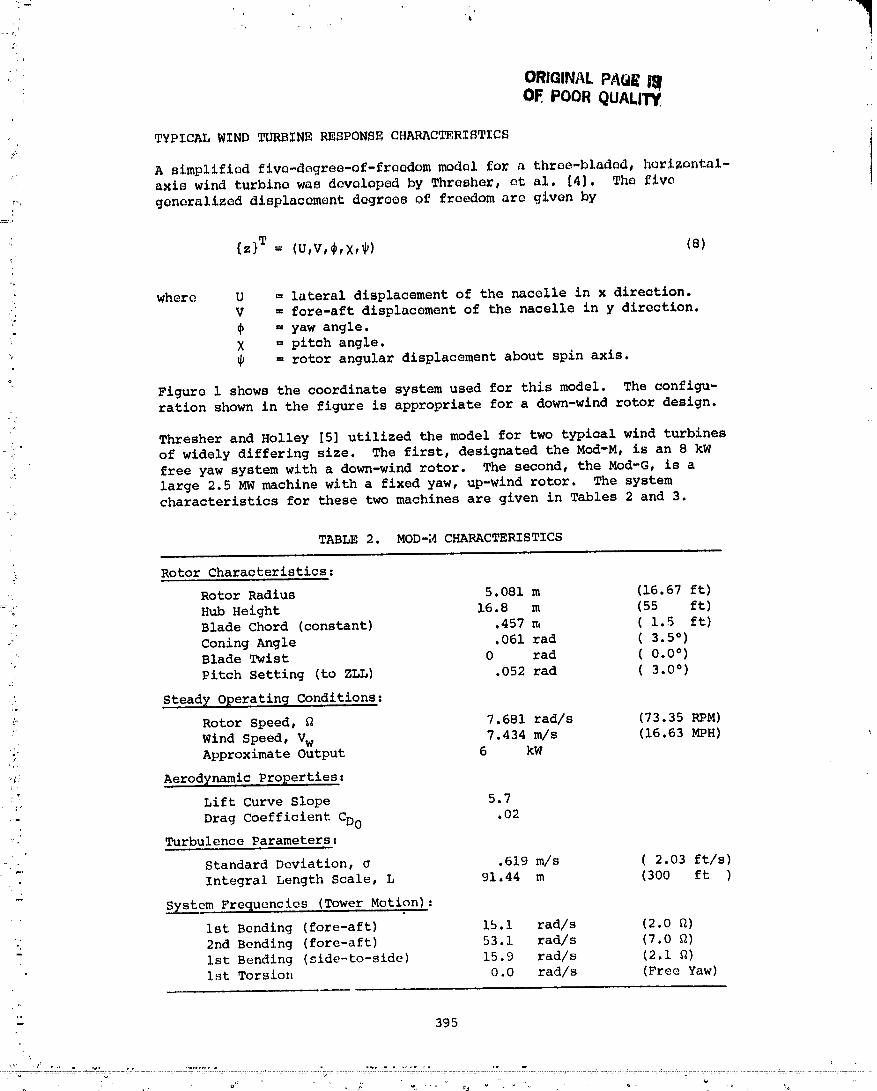
TYPICAL WIND TURBINE RESPONSE CHARACTERISTICS

A simplified five-degree-of-freedom model _or a three-bladed, horizontal-

axis wind turbln_ was developed by Thresher, et al° [4]. The five

?, generalized displacement degrees of freedom are given by

{z}T = (u,v,_,x,_) (8)

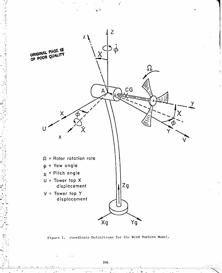
where U = lateral displacement of the nacelle in x direction.

:: V = fore-aft displacement of the nacelle in y direction.• _ = yaw angle.

X = pitch angle.

_ = rotor angular displacement about spin axis.

IFigure 1 shows the coordinate system used for this model. The configu-

ration shown in the figure is appropriate for a down-wind rotor design.

Thresher and Holley [5] utilized the model for two typical wind turbines

'. of widely differing size. The first, designated the Mod-M, is an 8 kW

_i free yaw system with a down-wind rotor. The second, the Mod-G, is a

large 2.5 MWmachine with a fixed yaw, up-wind rotor. The system

characteristics for these two machines are given in Tables 2 and 3.

TABLE 2. MOD-M CHARACTERISTICS

_ Rotor Characteristics:

-: Rotor Radius 5.081 m (16.67 ft)

". Hub Height 16.8 m (55 ft)

" Blade Chord (constant) .457 m ( 1.5 ft)

Coning Angle .061 tad ( 3.5 °)

. Blade Twist 0 tad ( 0.0 °)

Pitch Setting (to ZLL) .052 tad ( 3.0 °)

• _ Steady O_eratin _ Conditions:

_" Rotor Speed, _ 7.681 rad/s (73.35 RPM)

• Wind Speed, Vw 7.434 m/s (16.63 MPH), Approximate Output 6 kW

'_." Aerodynamic Properties:

_ Lift Curve Slope 5.7

- Drag Coefficient CD0 .02

Turbulence Parameters:

-.' Standard Deviation, _ .619 m/s ( 2.03 ft/s)

Integral Length Scale, L 91.44 m (300 ft )

System Frequencies (Tower Motion):

ist Bending (fore-aft) 15.1 rad/s (2.0 _)

" 2nd Bending (fore-aft) 53.1 rad/s (7.0 _)

ist Bending (side-to-side) 15.9 rad/s (2.1 R)

ist Torsion 0.0 rad/s (Free Yaw)

"" 395

00000005-TSB09

:' ORIGINALn_..,.i., J _

F , OF POORQUALITY

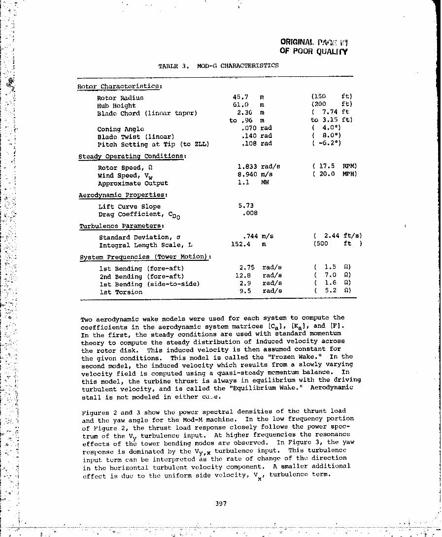
; TABLE 3. MOD-G CHARACTERISTICS

"_' Rotor Charaoterinticnl

_ ! Rotor Radius 45.7 m (150 ft)_r

:°""_ Hub Height 61.0 m (200 £t)

:_ Blade Chord (linear taper) 2.3G m ( 7.74 ft

' :,'_i to .96 m to 3.15 ft)

.[" Coning Anglo .070 red ( 4.0 °)

::_ Blade Twist (linear) .140 red ( 8.0")

'°' Pitch Setting at Tip (to ZLL) .108 red ( -6.2 e)

T Steady 08eratin _ Conditions_

" _ ' Rotor Speed, _ 1.833 rad/s ( 17.5 RPM)i 8.940 m/s ( 20.0 MPH)

,, .! Wind Speed, V w!_/ Approximate Output I.i MW

"; Aerodynamic Pro_erties_

" _i!:/i Lift Curve Slope 5.73..,% .008v._,o, Drag Coefficient, CD0

-:-i Turbulence Parameters_

-°!71/[ Standard Deviation, _ .744 m/s ( 2.44 ft/s): '.".' Integral Length Scale, L 152.4 m (500 ft )

"'_:"_ STstem Frequencies (Tower Motion)_

_ _ ist Bending (fore-aft) 2.75 rad/s ( 1.5 _)

_,'i'._. 2nd Bending (fore-aft) 12.8 rad/s ( 7.0 _)

_._ ist Bending (side-to-side) 2.9 rad/s ( 1.6 _)

i._.-"' ist Torsion 9.5 rad/s ( 5.2 _)

:"_.." Two aerodynamic wake models were used for each system to compute the

J'":':! coefficients in the aerodynamic system matrices [Ca], [Ka] , and [F].:i_ :_i_._." In the first, the steady conditions are used with standard momentum:j,/:

L_.....:_', theory to compute the steady distribution of induced velocity across"_""".': the rotor disk. This induced velocity is then assumed constant for

_..'"':' the given conditions. This model is called the "Frozen Wake." In the

'!"°'i:'.i/! second model, the induced velocity which results from a slowly varying

v_ velocity field is computed using a quasi-steady mementumbalance. InI' this model, the turbine thrust is always in equilibrium with the driving

_i:, turbulent velocity, and is called the "Equilibrium Wake." Aerodynamic--'.," stall is not modeled in either ca_.e.o i.:_

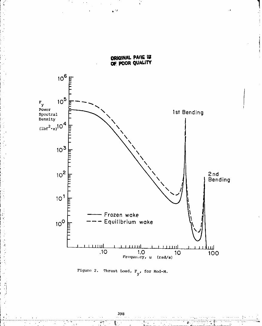
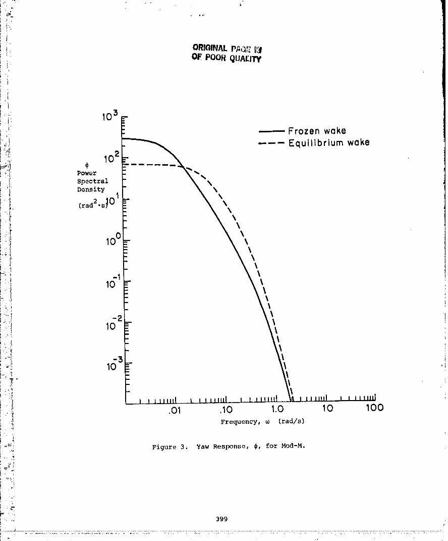
" I Figures 2 and 3 show the power spectral densities of the thrust load

._!.i_i..'i and the yaw angle for the Mod-M machine. In the low frequency portion

", of Figure 2, the thrust load response closely follows the power spec-

._.,_ trumof the Vy turbulence input. At higher frequencies the resonance

! effects of the tower bending modes are observed. In Figure 3, the yaw

o_.:._ response is dominated by the Vy,x turbulence input. This turbulenceinput term can be interpreted as the rate of change of the direction

&% _ in the horizontal turbulent velocity component A smaller additionalo_ _i effect is due to the uniform side velocity, V , turbulence term.

;'

,>_

i • ' " 397

..... _ ............... _ ......._:,_ _ _;..........................................._.......v..........:,:...........:........_:.........:i............._,:...................................................5........_....................................................................................................."..............................................

O0000005-TSBll

ORIGINAl,.PA_I__Bo17POORQUAI.ITY

OF POOROIJA[IW

:,, 1031__. l _ Frozen wake_ ------ Equilibrium wake, ,.,i. 102_:_1 _ ......_I Power • %

I Spectral %

!i Density

I \• \

,i.t (rad2"sgO \

_ 100 \. \ii!.r"% !:

°:i 10

!,

i' .01 .10 1.0 10 100' t

,, Fz'equency _ e (tad/s)

• _,

,_ Figure 3. Yaw Response, _, for Mod-M.

: 399

000000(')._-T.C:;R1

:- ORIGINALPAGEISOF POORQUALITY

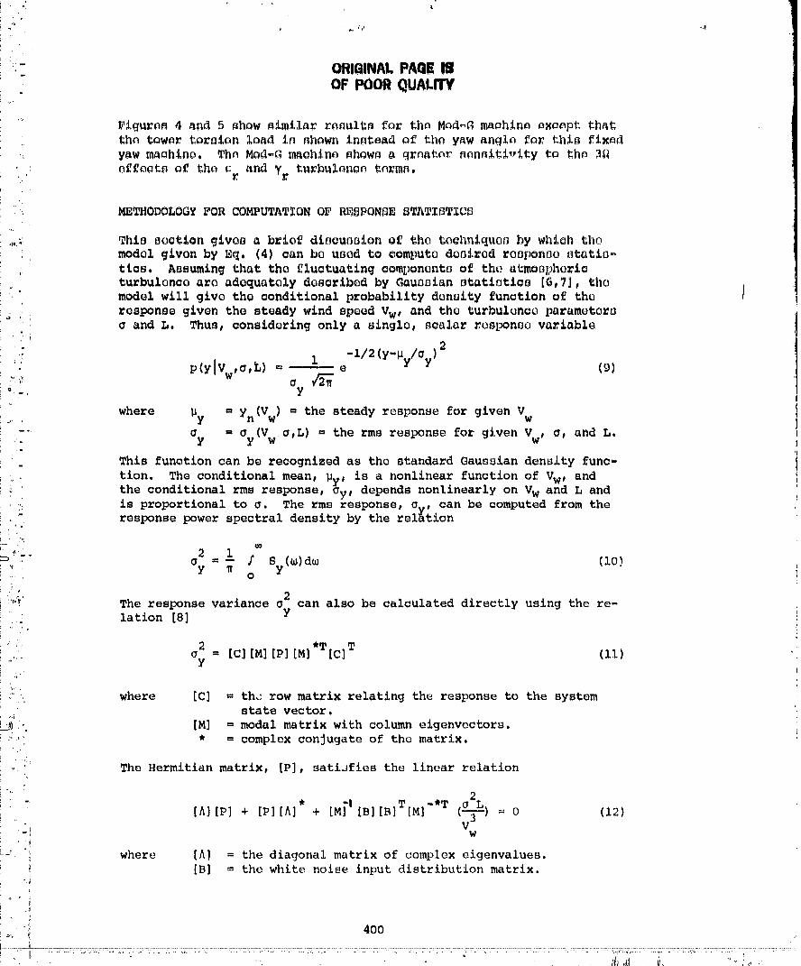
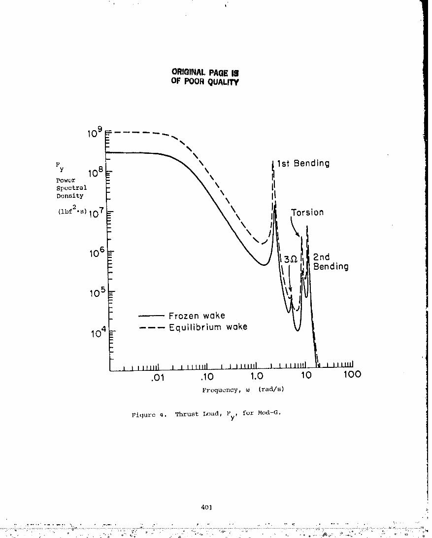
.... FigUreS 4 _nd 5 show _imilar results for the Mod_ maahln_ o_o_pt th_

the tower torsion load in shown Instead of the yaw anglo for thi_ fIxnd

•_ y_w,mchlno. The Mod-G machine shows _ greater sonslti-_ty to the 3_

: effects of the _ and Yr turbulnnoo tnrms.

METHODOLOGY FOR COMPUTATION OF R_SPONS_ STATiSTiCS

,,_,_ _his section gives a brief discussion of the toohniquoll by which the

model given by Eq. (4) can be used to compute doslrod ro0ponoo static-

,: tics. Assuming that the fluctuating components of the atmosphorlcturbulence arc adequately described by Gauooian statiotics [6,7), the

) model will give the conditional probability density function of the I

: response given the steady wind speQd Vw, and the turbul_nco parameterso and L. Thus, considering only a single, scalar resi_nso variable

2

: 1 -i/2(y-py/_y)_" p(ylVw,O,L) = -- e (_)

where py = Yn(Vw) = the steady response for given Vw

:?- _y = _y(Vw o,L) = the rms response for given Vw_'o, and L.

: This function can be recognized as the standard Gaussian denslty rune-

,... tion. The conditional mean, _y. is a nonlinear function of Vw, andthe conditional rms response, Oy, depends nonlinearly on Vw and L and

_: is proportional to o. The rms response, Or, can be computed from the: response power spectral density by the rel_tion

_ 2 1.... _ = -- I S (_)d_ (lO)

Y _ y i"/ , 0

/'" 2:'_' The response variance O can also be calculated directly using the re-. lation [8] y i

= [C] [M] [P][M]*T[c] T (ii)Y

o>, where [C] = th,:row matrix relating the respons_ to the system

•,_. state vector.

!-___!,'-. [M] = modal matrix with column eigenvectors.• = complex conjugate of the matrix, i

,_. The Hermitian matrix, [P], satiJfies the linear relation

/

• I T -*T eL! .. [A) [P) + [P] [A] + [M[ [B][B] [M] (_) = 0 (12)

-i Vw

L_' "_ where [A] = the diagonal matrix of complex eigenvalues.

[B] = the white noise input distribution matrix.(i

:_ 400

':_:- =:_"=: ::;=_ _'_:_:_: :_ ::_ "........ _ :: : =:: _:...... _........ :::""..... ".... _ ..... :: :=:: :::::=::_:: ,"=: ::: ...... = _::: : : __ : " i_'::__::: _::_::_:_ ::::":'_:_:_: ........ i.................

O0000005-TSB14

ORIGINALPAGEIJOF POORQUALITY

109 F ..... -......_ ,,\

1- ....... _-._,. ,\ ,. I

Fy 108 _--- \\ 1St BendingPower

m

Spectral

Density

(ibf2.s) 107: _\ Torsion

106 - I; _3_I 2nd: I I Bending

-- U Frozen wake

104 __-- -----" Equilibrium wake k,m

- i- 1 I IIIIILI I 1 Illlltl ._1 1 Illllll I I lllllll I Itluil

.01 .10 1.0 10 100Frequency, _ (tad/s)

Figure _. Thrust Load, Fy, for Mod-G.

4O]

_ _' ' "_"'" _'"" -'r" \, " ........ • -, .. o "

O0000005-TSC01

c'..

" ORIGINALPAGEiS.._ OF POORQUALITY

....,..- 1012I_

-, :0 '

' i. ,

;:" 011L \

_:,_,-. 1 _ _ \\ 1st Bending

_., - Power

. , ..,,,_' Spectral I_0

_ ':....ii' Density _ _'\ /I _

:.. (_t2._bf2..) \ I II

• io9 ", "-'Ilk3alll and

_. ending

2,;i.'::<.

.-_i iT'.,._ ,._

--'%/; .

;:,. -----'-- Fro e wake

:. :::. 106 --

m _

,,v./ ,

.=).G/-.

_,.:/ .01 .10 1.0 10 10 0

L-./"_.'. Frequency, _ (tad/s):-'jL.[i

: _:_.:!, .

: _:_. : Figure 5 Tower Torsion Load, Mz, for Mod-G:__..

4_

I/.

n /

':, 402

00000005-TSC02

i

i. . ORICINAI, PAGI" b_!,,. OF POUH QU/tLIIY

N=It't_l.luIILII=_lllill.r.l_Otlllil, IMI, nnd [A] di_l,qld mm.l.:In_,i.,'.l.yon the,

l)'ilFillllt_|:l_l'll V 4111tl ],,W

... NoW0 tltlllltllli' i|' LII (htlllFl'¢l to COlll|ltlt'(1 thi t p:L'Obabillt;y t.ha('_ y llxetli.ldtl d

• _'l,l'l.,*in el'it tx',=] value' yc. Th¢, _;andittonal prolx]bil.l.ty is qivon by

:... I'*'{y " yclVw,O,]'.,} '_ / t,(yJVw,O',l_)dy 1.1.:_)

• Sutmt.itutinq Eq, (_l) {nt'o Eq. 113) y[t_lds<

,_1," p,ly vIVw,,,,,i <re('>' "" '-- ,'T - ) (14)

.' %J

_'" 1 (') o-y;:12i ' whorl, tn't'1.) = _ f dy =-_the error funct.lon.i. /:;.::o

Tilt, tot.d,1 lu'olmbt]Jty is thus givon by

Pr{y "- yc) .:f f f (_I _ t,rf(_))P(Vw,O,L)dV dodL (Ib)o w,, o o o y

whet't, I_(Vw,¢,,L) _--the joint: lu:obabi[it:y density function of the' ix_sltlve wllld dnd ttlrbulence parameters.

b

-"i l"or coml,utationa] [*urlk_ses, the inte¢lral,J can be. approximated by dls-

!-":. CI't'I[.O.SUlOnIa[.I.OllS,.qO that

Yc-P

t_r{_, "_ _' } _'_ ,': (_ - _,rf(-%-JL))P(Vwj,%,L _) (16)_i ' i,k,_ 2 Y

whert, tht, subscripLs denote discrete v,ilues of the [_arameters associated

"7 with "count[nq bills." 'l'hevrobability required Is the jolnt probability

that Vw ts in bin i, 0 _.,_:iu bin k, and t, is it, bin _._.

i , Ulilortun¢it ely, cOral*lore data for d(,tt,iuninil%%1thi, joint density funci [on

lkn" the willd ilnd t.tit'btllt_liCt, t_aranlt,ti,rs it, %lt,llt, I'ally lackintl, lltlwever,

.._ llt,Vt,l',l I silul,[ifying dtl}ltlllillt iollS tllakt, all ,lt>}_roxinlate modt,1 }_ssiblu.

! ii ,ill ,t [llloltl,ht,t:[c bOtilld,ii:y lair't,! • Wi th tiOtlt'l.'_l I buoyalit ,,_tability tlit_

It_q,lrithlll[c lu'ofilt' h,ls llol,ll t'otlnd t.o ach,qtlatt, ly niodt, l. tllt_ varicltionof V with hoi<lht I'll. 'l_htil luodt'l ill of the lkU'lll

w

u, z-:' ,i.:-V .... _nl .... !.l--- 5-'-) 117)

it' tl.,i I""" t'%

wht'l't' tl, I't'lct i<_ll re'it,city.., _" lit,iqht ,Ibovt, I he _ll'_Uilld.

I; llOillill,il h_.|q|il w}1¢'1"¢, V t) (olt,.'ll Z¢>l'<l).II W

>>

40 I

00000005-TSC03

..,

.,,.,

,.t_,';

: OIRIG."Ag...l;%'_,.,il__;_'_- Z = terrain roughness length. OF POOR QUAI.[II'_

0 O

Frost, et al. [i0] recommend the Weibull probability distribution for

_ the steady wind speed at the reference height of i0 m. Thus solving==

Eq. (17) for u, when z = zr i0 m yields

tZ-Z +Z

i: n o),,_? _n( z._. V = V o (18)_o:...._ W r z -z +z'_" in( r n o)

. ," O

_!;.;_.: where V r '= Vw at the reference height.

=_." z = reference height.

.... i_, Since Vw and Vr are linearly related, Vw also satisfies the Weibull=:i,.,, distribution which can be differentiated to give the density function

;.:, of the form

_2°_i" k

pCVw) k Vwk-1e-CVw/VoI= (_'::') (191'_:L",. 0 0

where k = a site parameter (= 2)._ V

_:'d. ": WV =

=_. o r(1+ l)::_:',;.: V = annualkmean wind speed at the desired height.w

"-:<_'- F (•) = gamma function.

" The annual mean wind speed at the desired height can be found from the

.,...,_ value at the reference height by the use of Eq. (18).

__'< The rms, turbulent component velocity, _, is found to be highly corre-

.;': lated with the steady wind speed. Panofsky, et al. [ii] give the re-

'._ lation

:, ..,: 0 = 2.3 U, (20)

.... so that when Eq. (17) is used for u,,

"_ ' 0.92."., ' o = V (21)

•, Z-Z +Z W

' in( "' r o)." ' Z", ' O

- The turbulence integral scale, L, is much less understood. Most evi-

, . dence indicates that it is independent from the steady wind speed, Vw,"_ and the variance, 02 . Several authors [12,13,14] recommend different

-" power laws for the variation of integral scale with height. However,

these relations are inconsistent and the experimental data exhibit

_... wide scatter. It is highly recommended that an experimental program be

404

.....:_:....._.........................................................................................................................................................................................................................................................................<"

00000005-TSC04

. r._

.__ undertaken to deteFmine an appropriate height scaling law and to accountstatistically for the variation observed at a given height. In the

interim, we will assume the integr_l scale is deterministic and satisfies

the height relation

: L = L (22)r z

r

.:_' where Lr = a site parameter (= 65 m).

! zr = reference height = i0 m.

Using these simplifying approximations for the parameter models, the

statistical procedure given by Eq. (15) reduces to

1 Yc -_

p(Vw)dV (23); Pr{y > yc} = _ (_- erf,: o y

where p(V w) is given by Eq. (19).

The quantities _y and _v will be complicated functions of Vwgiven by' the model of the turbin_ response, with Eqs. (21) and (22) used for the

°i parameters _ and L. Obviously, numerical procedures would be used to

; perform this computation.

:_ ESTIMATION OF MODEL PARAMETERS FROM FIELD DATA

Since the steady wind and turbulence parameters, Vw, _, and L, criti-

_ cally affect the statistics of the response, it is highly desirable to

have a reliable method for extracting the parameters from real field

data• One such method is the equation error method [15]. Basically,

the method determines a set of parameter values which minimize the

,: difference between the data and predicted values based on the model

equations• The resulting parameters will then serve to characterize the

turbulence sample observed. A whole collection of such parameter values

will then give the required statistical information discussed in the

previous section.

Before proceeding to give the detailed procedure for estimating the mean

! wind and turbulence parameters, a brief description of the equation

error method will be given. Suppose we have an accurate, noise-free

measurement of a random process, u, modeled by the stochastic differen-

tial equation.

= au + bw (24)

where w = white noise with flat PSD = Swa,b = model parameters.

_;. ORIGINALPAGE18oF eooRQUALIFY

:/_ The measurements will be a set of N values, u(i) taken at discrete

times with a constant time interval, T, between measurements. The• continuous time model can be converted to the discrete time form

" u(i+l) = eaT u(i) + _(i) (25)

_"'_ where _(i) = a random sequence of uncorrelated values.q

i The variance _ of _(i) is found by matching the stationary variance of i.. u(i) and u(t). Thus, from Eq. (25)

2aT_ . E[u2(i+l)] = e E[u2(i)] + E[_2(i)] (26)i

. !_ which when solved yields

:_:_ 2 A 2 e2aT) 2:_:i _ = E[_ (i)] = (i- o (27)i ._ _ U

! From Eq. (24) (assuming a < 0),

J i 2a_2 + b2S = 0 (28):.., U W

_ Using Eq. (28) in Eq. (27) yields

2aT) b 2./ o2_ = (i - e (- _a Sw) (29)

Now, since u(i+l) and u(i) are linearly related and the noise term is

sequentially uncorrelated, standard regression methods [16] can be

used to estimate eaT and _ from the data sequence. Thus, we choose

-j the parameter, a, to minimfze the estimated variance

N-I^2 1 aT 2

o__ = _ E (u(i+l) - e u(i)) (30)i=l

b2Sw , is determined from Eq. (29)The product,

b2S = (31)' w 2aT_ 1 - e

' separately.

i It is impossible to estimate b and Sw

•'i With the mathematical preliminaries out of the way, let us ret_irn to

the turbulence parameter estimation problem. Suppose we have two

406

00000005-TSC06

!-, .z

,:,. ORIGINAL PAGE |5' OFpOORqUALN'Y

:! tj'_1 propeller type anemometers set up to measure orthogonal horizontal i!

i components of the wind. Let vl(i) and v 2 (i) be sequences of measure- I' I ments taken from the anemometers. The first step in the procedure is to

::: find the steady wind speed and direction. Thus, dotermine .

'?P Nu, i

= - 7_ vl(i)/::['_ <Vl> N i=l

,/i.:[ (32 )

1 N= -- v2(i )

= ' <v2> N iY'=l

!i !I Now,

---:'_'_:'! V = /<Vl >2 + <V2>2_: ':, w (33)

....._£ .. _ = tan -I <v2

<v 1=L#_]:_',_i. The lateral and longitudinal turbulence components are thus determined

_.':_!:_[ from_:_.:•

_,!jj: V (i) = v2(i) cos_- vl(i) sin_-:_:.._ X (34)

_"_ V (i) = vl(i) cos_ + v2(i) sin#- V

• 'C

":-:'. The next step is to determine the parameter, L, using the equation error

_ regression procedure. According to the model developed by Holley [17],

the lateral and longitudinal components of the turbulence satisfy the

/_'c_r stochastic differential equations

.I, 2V 2o.:._: 2V W

,._.. _' = ----_wv +--w 1"_' X L X L

o ; (35)

•:."t V w/2 V 2

i, V = --_w V + W 2"!_ y L y L

=.;:!:o_ where w I and w 2 are independent white noise processes with equal power.;',} = O2L/V 3_" } spectral densities, Sw - w"

o jJ Applying the equation error regression technique of Eq. (30) and normal-

:] izing each of the equation errors by the variance gives the variance° I estimate

•; "2 ^2

:_" ^2 1 °l °2

'_ o = z"/ ( ' -4V _/L + -2V T/L)/ (36)w w

" l-e l-e

; 407

00000005-TSC07

_ _; , tJ_

t

_: _i ORIGINALPAGEI_:/::i QUALITY-.i: ._ OF POOR

:'" ^2 i .-i -2v./L 2'" Em

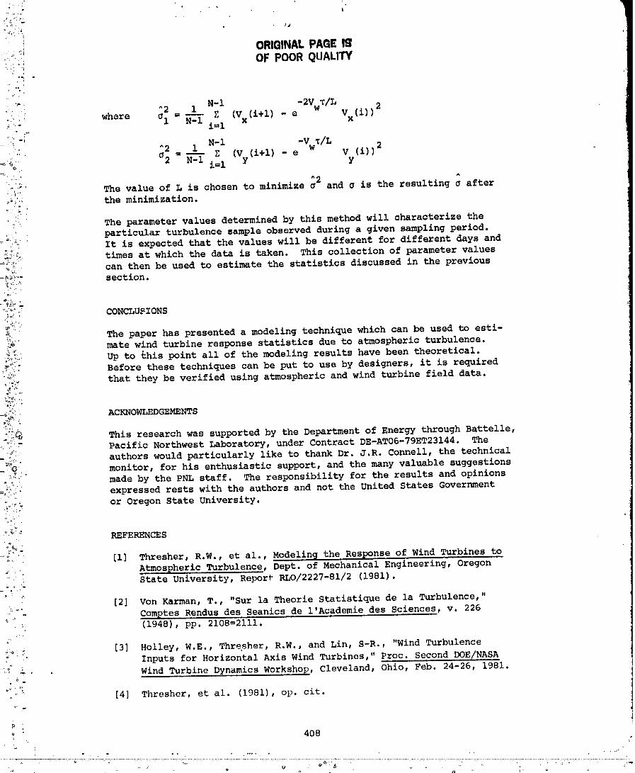
._";'.....'.'i where Cl _N-I g (Vx (i+1) - e Vx (i))i=l

-':-" ^2 l .-i -v_IL (i))2..... a 2 =- Z (Vy(i+l) - e V,,," N-I i=l Y

.'.- A,,. A 2

;_:'." The value of L is chosen to minimize c and c is the resulting c after,_::: the minimization.

c ._' '•... The parameter values determined by this method will characterize the

..,i.". particular turbulence sample observed during a given sampling period.

_".!_,:ii Zt is expected that the values will be differen_ for different days andi:,_:: times at which the data is taken. This collection of parameter values

2:, can then be used to estimate the statistics discussed in the previous-_-__:'- section._.,.'...

_j:._ co_cnusz0.s

_ The paper has presented a modeling technique which can be used to esti-

._ mate wind turbine response statistics due to atmospheric turbulence.

_:'_"_ Up to this point all of the modeling results have been theoretical.

_"" Before these techniques can be put to use by designers, it is required

-:'_' that they be verified using atmospheric and wind turbine field data.

-_ ",. ACKNOWLEDGEMENTS

2_i_i_ This research was supported by the Department of Energy through Battelle,Pacific Northwest Laboratory, under Contract DE-AT06-79ET23144. The

= o...,. authors would particularly like to thank Dr. J.R. Connell, the technical_ •

= _ . monitor, for his enthusiastic support, and the many valuable suggestions

_. made by the PNL staff• The responsibility for the results and opinions

7-;_!-i__:i' expressed rests with the authors and not the United States Government"L.__ or Oregon State University•

°_"'': REFERENCES

..... [i] Thresher, R.W., et al., Modelin_ the Response of Wind Turbines to

_.', Atmospheric Turbulence, Dept. of Mechanical Engineering, Oregon'. State University, Repor_ RLO/2227-81/2 (1981).

[2] Von Karman, T., "Sur la Theorie Statistique de la Turbulence,"

-' Comptes Rendus des Seanics de l'Academie des Sciences, v. 226%

(1948), pp. 2108=2111.

._:o,i [3] Holley, W.E., Thresher, R.W., and Lin, S-R., "Wind Turbulence

° " Inputs for Horizontal Axis Wind Turbines," Proc Second IX)E/NASA

.... Wind Turbine Dynamics Workshop, Cleveland, Ohio, Feb. 24-26, 1981.o

o_ [4] Thresher, et al. (1981), op. cit.

: 408

00000005-TSC08

[5] Thresher, R.W. and Holley, W.E., The Rest?rise S_sltivit_ of Wind

Turbines to Atmospheric Turbulence, Dept. of Mechanical Engineering,Oregon State University, Report RL0/2227-81/I (1981).

. [6] Connell, J.R. and Powell, D.C., Definition of Gust Model Conce_t s

; and Review of Gust Models, Battelle Pacific Northwest Laboratory,

Report PNL-3138 (1980), pp. 6-8.

,:. [7] Etkin, B., Dynamics of Atmospheric Flight, Wiley (1972), p. 532.

[8] Kwakernaak, H. and Sivan, R., Linear optimal Control S_stems, Wiley

*' (1972), pp. 103-104.

; [9] Lumley, J.L. and Panofsky, H., The Structure of Atmospheric Turbu-

"_ lence, John Wiley & Sons (1964), p. 103.

o

[i0] Frost, W., Long, B.H., and Turner, R.E., En_ineerin 9 Handbook on

the Atmospheric Environmental Guidelines for Use in Wind Turbine[

_7_ Generator Development, NASA TP 1359 (1978), p. 2.48.

:_ [ii] Panofsky, H.A., et al., '_The Chazacteristics of Turbulent Velocity

; Components in the Surface Layer Under Convective Conditions,"

_ Boundary-Layer Meteorology, v. ii (1977), p. 357.

=_ [12] Counihan, J., "Adiabatic Atmospheric Boundary Layers: A Review

and Analysis of Data from the Period 1880-1972," AtmosphericEnvironment, v. 9 (1975), p. 888.

o_ [13] Etkin, B. (1972), op. cir., p. 542.

[14] Frost, W., et al. (1978), op. cit., p. 4.18.

" [15] Eykhoff, P., System Identification, Wiley (1974), pp. 228-277.

[16] Goodwin, G.C. and Payne, R.L., Dznamic S_stem Identification,

Academic Press (1977), pp. 22-41.

_i [17] Holley, et al. (1981), loc. cir.

409

00000005-TSC09