Embed Size (px)
Citation preview
NSF/RA-800625
PB82-141844
80-SM-1410. Project/Task/Work Unit No
11. Conlract(C) or Grant/G) No.'i ng
(C)
(G)PFR7822865
~nce (EAS)
13. Type of Report & Period Cc
14.
------------------~---------
---------_.- . - ..
1S Program (OPRM)~nce Foundati onDC 20550 .- ._---------
elastic models were developed for evaluating naturalbration of a wide class of earth dams in a directionThe nonhomogeneity of the dam materials was consideredfal (axial) deviations. Dynamic properties of three refornia estimated from their earthquake records and the
'" I .1..' +' ft ..... 0..,.. +hc. CllaaoctQd model
PRINCETON UNIVERSITY
Department of Civil Engineering
IltPROOUOEO BYNATIONAL TECHNICALINFORMATION SERVICE
u.s. DEPARTMENT OF COMMERCESPR1N9FIElD. VA 22161


50272 -, 01
REPORT DOCUMENTATION \1. REPORT NO.PAGE NSFjRA-800625
4. Title and Subtitle
Earthquake Induced Longitudinal Vibration in Earth Dams
3. Recipient's Accession No,
ff!' f;", ~:Jfi ,~'-~ ~:~: ='.i ~l i~, ~,liJ~G& .~ is~~'" c; :> _
5. Report Date
December 1980
11. Contract(C) or Grant(G) No,
10. Project/Task/Work Unit No,
8. Performine Organization Rept, No,
80-SM-147. Author(s)
A.M. Abdel-Ghaffer9. Performing Organization Name and Address
Princeton UniversityDepartment of Civil EngineeringPrinceton, NJ 08544
6.
(C)
(G)
008196
PFR7822865
12. Sponsoring Organization Name and Address
Engineering and Applied Science (EAS)National Science Foundation1800 G Street, N.W.Washington, DC 20550
13. Type of Report & Period Covered
14.
16. Abstract (Limit: 200 words)-------- ------
15. Supplementary Notes
Submi tted by: Communications Program (OPRM)National Science FoundationWashington, DC 2__05~ _
- -----------------1
Two-dimensional analytical elastic models were developed for evaluating naturalfrequencies and modes of vibration of a wide class of earth dams in a directionparallel to the dam axis. The nonhomogeneity of the dam materials was considered aswell as both shear and normal (axial) deviations. Dynamic properties of three realearth dams in Southern California estimated from their earthquake records and thedynamic test results of one dam, are compared with those from the suggested models.It was found that the models in which both the shear modulus and the modulus ofelasticity of the dam material vary along the depth provide the most appropriaterepresentations for predicting the dynamic characteristics. The theoretical resultsfrom some of the models compared favorably with the experimental and earthquake data.An analysis of real earthquake performance of an earth dam, in the longitudinaldirection, yielded data on the shear moduli, damping factors, and nonlinear constitutive relations for the dam materials; Ramberg-Osgood nonlinear stress-strain curveswere then fitted to these data. As a result of the study, a qualitative picture ispresented of the distribution of dynamic str~ins and stresses and stresses within anearth dam during an earthquake.
1-------------------------------------------------,17. Document Analysis ao Descriptors
Earthquake resistant structuresEarth damsDynamic structural analysisModel tests
b. Identifiers/Open·Ended Terms
Southern CaliforniaA.M. Abdel-Ghaffar, jPI
c. COSATI Field/Group
18. Availability Statement
Stress-strain curvesShear modulusModulus of elasticity
19. Security Class (This Report) 21. No. of Pages
NTIS 1----------------11----------
(See ANSI-Z39,18)
20. Security Class (This Page)
See InstructIons on Reverse
22. Price
OPTIONAL FORM 272 (4 77)(Formerly NTIS-35)Department of Commerce


PRINCETON UNIVERSITYCIVIL ENGINEERING DEPARTMENT
STRUCTURES AND MECHANICS PROGRAMS(Earthquake and Geotechnical Engineering)
EARTHQUAKE INDUCED LONGITUDINAL VIBRATIONIN EARTH DAMS
by
Ahmed M. Abdel-Ghaffar
REPORT NO. 80-SM-14
DECEMBER 1980
A Report on Research Conducted under Grant
from the National Science Foundation
PRINCETON, NEW JERSEY


This report is based on research conducted under Grant No. PFR7822865 from the National Science Foundation. Any opinions, findings andconclusions or recommendations expressed in this publication are thoseof the author and do not necessarily reflect the views of the NationalScience Foundation.


iii
TABLE OF CONTENTS
Page
Acknowledgments
Abstract
CHAPTER
CHAPTER I I
INTRODUCTION
FREE LONGITUDINAL VIBRATION OF NONHOMOGENEOUSEARTH DAMS11-1. Simplifying Assumptions and Practical
Considerations11-2. Free Vibration Analysis
2
4
10
1017
CHAPTER I I I COMPARISON BETWEEN THE RESULTS OF THE PROPOSED MODELSAND REAL OBSERVATIONS 38I 11-1. Earthquake Response Records 38I I 1-2. Full-Scale Dynamic Test Results 49
CHAPTER IV EARTHQUAKE-INDUCED LONGITUDINAL STRAINS AND STRESSESIN NONHOMOGENEOUS EARTH DAMS 58IV-I. Earthquake Response Analysis 581V-2. Dynami c Shear Stra i ns and Stresses 63I V-3. Dynami c Axi a 1 (Norma 1) Stra i ns and Stresses 72IV-4. Utilization of Response Spectra 79
CHAPTER V IDENTIFICATION OF CONSTITUTIVE RELATIONS, ELASTICMODULI, AND DAMPING FACTORS OF EARTH DAMS FROM THEIREARTHQUAKE RECORDS 87V-I. Basis of the Analysis 87V-2. Application of the Analysis 90
V-2-1. Longitudinal Dynamic Shear Stress-StrainRelations for Santa Felicia Earth Dam 90
V-2-2. Shear Moduli and Damping Factors forSanta Felicia Earth Dam 109
V-2-3. Axial Strains and Stresses of SantaFe1icia Dam 114
CONCLUSIONS
References
APPENDIX A: Standard (Unfiltered) Earthquake Records ofSanta Felicia Dam
APPENDIX B: Tables of Shear Strains and Stresses Induced by theTwo Earthquakes
117
118
121
127


ACKNOWLEDGMENTS
This research was supported by a grant (PFR78-22865) from the National
Science Foundation (Research Initiation in Earthquake Engineering Hazards
Mitigation). with Dr. William W. Hakala as the Program Manager.
The author is grateful to Mr. Aik-Siong Koh. a graduate student in
the Civil Engineering Department at Princeton University. for his research
assistance and for the computer-plotting of most of the curves in this report.
The assistance provided by both the Department of Materials Engineering
at the University of Illinois at Chicago Circle (1978-1979) and the Department
of Civil Engineering at Princeton University (1979-1980) is greatly appreciated.
Appreciation is extended to the School of Engineering and Applied Science at
Princeton University.
The author also acknowledges the valuable discussions and suggestions
given by Dr. Attila Askar of the Bagazici University in Turkey.
Sincere thanks are given to Ms. Anne Chase for her skillful typing of
the manuscript and for help in preparing the final report.

2
ABSTRACT
Two-dimensional analytical elastic models are developed for evaluating
dynamic characteristics, namely natural frequencies and modes of vibration
of a wide class of earth dams in a direction parallel to the dam axis. In
these models the nonhomogeneity of the dam materials is taken into account
by assuming a specific variation of the stiffness properties along the
depth (due to the continuous increase in confining pressure). In addition,
both shear and normal (axial) deformations are considered. Cases having
constant elastic modul i, linear and trapezoidal variations of elastic modul i,
and elastic moduli increasing as the one-half, one-third, two-fifths, and a
general (~/m) th powers of the depth are studied. Dynamic properties of three
real earth dams in a seismically active area (Southern Cal ifornia) estimated
from their earthquake records (input ground motion and crest response in
the longitudinal direction) as well as results from full-scale dynamic
tests on one of these dams (including ambient and forced vibration tests)
are compared with those from the suggested models. It was found that the
models in which the shear modulus and the modulus of elasticity of the dam
material vary along the depth are the most appropriate representations for
predicting the dynamic characteristics. The agreement between the experi
mental and earthquake data and the theoretical results from some of the
models is reasonably good. Based on the analytical models, a rational pro
cedure is developed to estimate dynamic stresses and strains and correspond
ing elastic moduli and damping factors for earth dams from their hysteretic
responses to real earthquakes, utilizing the hysteresis loops from the
filtered crest and base records. This leads to a study of the nonlinear
behavior in terms of the variation of stiffness and damping properties with

3
the strain levels of different loops. Finally, an analysis of real earth
quake performance of an earth dam, in the longitudinal direction, yields
data on the shear modul i, damping factors, and nonlinear constitutive rela
tions for the dam materials; the Ramberg-Osgood nonlinear stress-strain
curves are then fitted to these data.


4
CHAPTER
ItlTRO DUCT ION
Designing a dam to resist earthquake damage is probably one of the most
difficult tasks to be faced by the geotechnical and earthquake engineer.
The information available concerning the performance of earth dams in par
ticular during earthquakes is meager and offers little assistance to engineers
planning a dam in a region of seismic activity. As relatively few earth dams
have been subjected to strong earthquakes, it is dangerous to draw any
specific conclusions regarding their performance or the 1ikel ihood of any
particular modes of damage to such dams during strong ground motion. How
ever, the few existing recordings on and near dams may be of assistance in
giving some indication of performance characteristics in particular instances.
In the majority of earth dams shaken by severe earthquakes, two primary
types of damage have occurred (10,15,20,24,29,30): longitudinal cracks
at the top of the embankment and transverse cracks sometimes accompanied by
crest settlement. The longitudinal cracks appear to have been caused primar
ily by the horizontal component of the earthquake motion in the upstream
downstream direction, that is, the direction perpendicular to the longitudinal
axis of the daM. In contrast, transverse cracking of an earth dam can result
from longitudinal dynamic strains induced by earthquake motion in the
longitudinal direction (as well as from differential settlements). Such
cracks are of concern because they present a path for water to flow through
the dam's core.
Over the last two decades, much emphasis has been placed on the dynamic
response analysis of earth dams and their safety against earthquakes. Although
some progress has been made in the development of analytical and numerical
5
techniques (9,11,12,13,14,17,10,19,21 t22,23,24,2C) for evaluating the
response of earth dams subjected to earthquake motions, these techniques
are still in a rudimentary state of development. For instance, the existing
analytical techniques for earth dams still assume uniform shear beam, elastic
behavior, with the nature of the response restricted to horizontal shear
deformation in the upstream-downstream direction. Due to these restrictive
assumptions, the dynamic response analyses have many 1imitations and cannot
be used to examine the nature of stress distribution within an earth dam due
to longitudinal or vertical ground motion. In addition, a three-dimensional
finite element or finite difference technique would be very costly.
Although the existing dynamic analyses of the upstream-downstream motion of
an earth dam (Refs. 10 to 15, 19 t and 20) have the most notable importance to earth-
quake resistant design, there can be little doubt that the problem of earthquake
induced strains and stresses in earth dams from longitudinal vibration should
be of vital concern to earthquake and soil engineers. The importance of this
type of vibration is demonstrated by the following points:
1. Transverse cracking of an earth dam may result directly from the
large dynamic strains induced by the earthquake itself. Cracks that
reach the core would reduce the structural strength of the dam and
could lead to concentrated leaks resulting in eventual failure of
the dam.
2. Differential settlement of an earth dam may contribute significantly
to transverse cracking. The portions located close to the abutments
and, sometimes, the central portion of the dam are subjected to
tensile strains when the dam is deformed by differential settlement.
The levels which these strains reach are dependent upon the geometry
and relative compressibility of the foundation, abutments and embank-

6
ment. When the dam is then shaken by an earthquake, the additional
dyna~lic strains may cause cracks to develop even if the additional
strains are not large. This is explained by the fact that the initial
strains caused by differential settlement may not be apparent until
triggered or augmented by the e2rthquake. Figure 1.1 illustrates the
contribution from both the strains induced by differential settleme~t
and the dynamic strains induced by earthquake longitudinal excitation.
3. In all cases where earth dams have been seriously damaged durin; an
earthquake, the dams were constructed without the use of present
compaction control techniques. However, there is evidence to support
the contention that even a large, well-constructed, modern earth dam
can be cracked transversely by an earthquake. The San Fernando
earthquake of February 9, 1971 (ML = 6.3) caused a transverse crack on
the Santa Felicia Dam crest at the east abutment, Fig. 1.2, (Refs. 1,4).
This dam is comparatively large (236.5 ft high) and was constructed
>,ith modern design details and construction methods. The depth of
the crack, approximately one-sixteenth of an inch in width, is not
known. Investigation has impl ied that this narrow crack was caused
by the dynamic strains induced by longitudinal vibration result-
ing from the earthquake and not by any settlement. Fortunately, the
crack does not seem to be structurally significant.
This report develops analytical elastic models for evaluating the dynamic
characteristics of nonhomogeneous earth dams such as natural frequencies and
mode shapes of vibration in the direction parallel to the dam axis. Both
shear and axial deformations are considered, and the variation of stiffness
properties along the depth of the dam is taken into account. Comparison of
both real earthquake observations of three earth dams and experimental results

OPE
NC
RAC
KS'"
.......
,/
"
~~
..E
AR
THQ
UA
KE
.._
----
LON
GIT
UD
INA
LM
OTI
ON
CO
MP
RE
SS
I8LE
ALL
UV
IUM
LON
GIT
UD
INA
LS
EC
TIO
NS
.-
EXAG
GER
ATED
CR
EST
SE
TTLE
ME
NT
./'-
TEN
SIO
NZO
NES
",/'
""
TEN
SIO
NZO
NE
S./
-.....
...,I
-
PLA
NVI
EWS
OP
EN
CR
ACKS
STR
ES
SO
FFO
RC
E
•S
TRA
INO
R•
DE
FLE
CT
ION
BEFO
RE
EAR
11-tQ
UAK
E
STR
ESS
OF
FOR
CE
FAIL
UR
E
••
STR
AIN
OR
DE
FLE
CTI
ON
AF
TE
RE
AR
THQ
UA
KE
'-J
TY
PIC
AL
TRA
NS
VE
RS
EC
RA
CK
SIN
EA
RTH
DA
MS
DU
ETO
DIF
FE
RE
NT
IAL
SE
TT
LEM
EN
TA
ND
EA
RTH
QU
AK
ELO
NG
ITU
DIN
AL
EX
CIT
ATI
ON
S
Fig
.I.
IE
ffects
of
dif
fere
nti
al
sett
lem
en
tsan
dea
rth
qu
ake
shak
ing
s.

8
SANTA FELICIA EARTH - DAM
o !OOft~
PLAN VIEW
Continuationof crock inoverburden
Upstream
Downstream
East
Abutment
5eismoscope5-6
Fig. 1.2 The crack at the east abutment of Santa Felicia Dam as aresult of the San Fernando earthquake of February 9, 1971.

9
(see Refs. 1.3.4.6.7.8) with the models' theoretical results have confirmed
that these models are accurate enough to be used for estimating earthquake
induced longitudinal strains and stresses. In addition, the models and the
full-scale response results help to reveal differences in the dynamic proper
ties of dams under different loading conditions. Based on the analytical
models, a rational procedure is developed to estimate dynamic stresses and
strains and corresponding elastic moduli and damping factors for earth dams
from their hysteretic responses to real earthquakes. utilizing the hysteresis
loops from the filtered crest and base records. This leads to a study of the
non1 inear behavior in terms of the variation of stiffness and damping proper
ties with the strain levels of different loops. The report also uti1 izes
the standard response spectra for estimating maximum earthquake-induced
longitudinal strains and stresses. Finally, an analysis of real earthquake
performance of an earth dam, in the longitudinal direction, yields data on
the shear modul i. damping factors, and nonlinear constitutive relations for
the dam materials; the Ramberg-Osgood nonlinear stress-strain curves are
then fitted to these data. Although the assumption of elastic behavior
during earthquakes is not strictly correct for earth dams. it provides a
basis for establishing the natural frequencies of the dam, and it gives at
least a qualitative picture of the distribution of dynamic strains and
stresses within an earth dam during an earthquake.
10
CHAPTER II
FREE LONGITUDINAL VIBRATION OF NONHOMOGENEOUS EARTH DAMS
I I-I. Simpl ifying Assumptions and Practical Considerations
In view of the fact that earth dams are large three-dimensional struc-
tures constructed from inelastic and nonhomogeneous materials, the determination
,of their dynamic characteristics such as the natural frequencies and modes
of vipration is extremely difficult. As a result some simplifying assumptions
are introduced.
1. The dam is represented by an elastic wedge of finite length (with
symmetrical triangular section) in a rectangular canyon, resting on
a rigid foundation (Fig. 2.1). This model is similar to the one often
used to evaluate the dynamic characteristics of dams in the upstream-
downstream direction (9,11,13,18,21,23). Closed form mathematical
solutions for canyons of other shapes such as triangular, trapezoidal
or parabolic are extremely difficult. Hence, in order to make use of
the proposed solutions it is necessary to approximate a given dam's
canyon shape to an equivalent rectangle.
2. The dam is modeled by a nonuniform elastic material that has uniform
mass density p, a nonuniform cross section and variable stiffness
or elastic modul i (G and E: the shear and elastic modul i) along
the depth. Although the actual variation with depth (which is a
function of the soil type, the method of construction and the
geometry of the dam) has not been accurately measured in the field,
some efforts (l,h,16,19,21,23) are encountered in the literature

11
b b
ELASTIC TRIANGULAR WEDGEIN A RECTANGULAR CANYON
y,v
FORCES ACTING ON ANELEMENT IN THE DAM
zdz r
i~~.. x,U
Y LINEAR AND NONHOMOGENEOUS
dy,MATERIAL
~y,v
~y RIGID BEDROCK
.1-l- I-b b L
Fz +d{FZl
Fig. 2.1 The model considered in the longitudinal vibration analysis.
12
where the soil stiffness has been shown to vary in a continuous
manner due to the continuous increase in normal stresses (or confin-
ing pressure). The continuous variation of soil stiffness may be
represented by the following suggested relationships (Fig. 2.2):
A. Constant shear (or elastic) modulus (as a first order approximation):
G(y) G = constant. (2.1)
Dams constructed of homogeneous compacted earth fil I consisting
of material which is cohesive in nature cant at first approxima-
tion t be assumed to have a constant shear modulus (23).
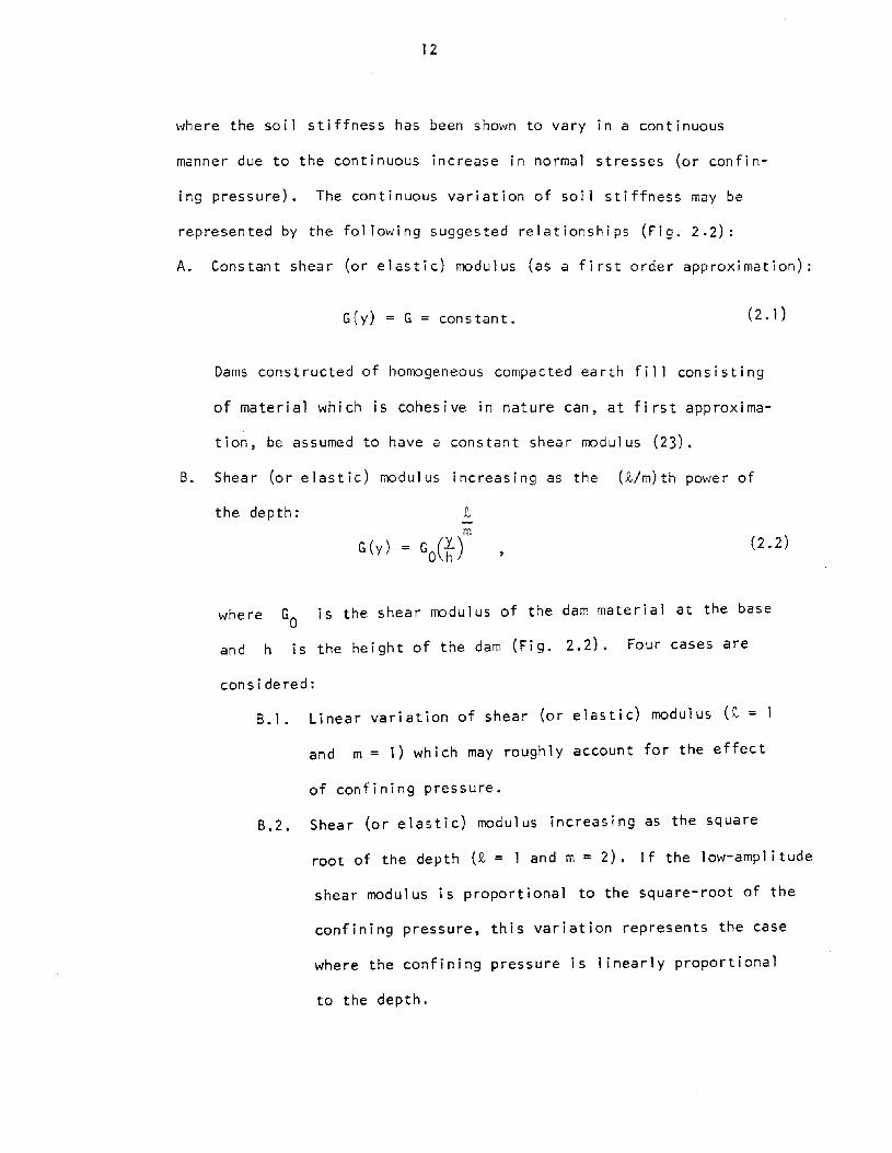
B. Shear (or elastic) modulus increasing as the (£/m)th power of
the depth:
(2.2)
where GO is the shear modulus of the dam material at the base
and h is the height of the dam (Fig. 2.2). Four cases are
considered:
B.l. Linear variation of shear (or elastic) modulus (t = 1
and m = 1) which may roughly account for the effect
of confining pressure.
B.2. Shear (or elastic) modulus increasing as the square
root of the depth (£ = 1 and m = 2). If the low-amplitude
shear modulus is proportional to the square-root of the
confining pressure t this variation represents the case
where the confining pressure is linearly proportional
to the depth.

13
-~......~ 0.2t;
~ 0.3
~0.4LLJ
a:l
::J:~
0.5Cl.LLJ0
(/)0.6(/)
LLJ....J G=Go(y/h)z0 0.7V5zLLJ~
0.8is
0.9
1.0
Fig. 2.2 Variation of stiffness properties alongthe depth of the dam.

14
B.3. Shear (or elastic) modulus increasing as the cube root
of the depth (t = 1 and m = 3). For earth dams consist-
ing of cohesion1ess material, this case is most
appropriate, because it has been shown that for such
materials the shear modulus is approximately propor-
tional to the cube root of the confining pressure
(16,17,23,31) •
B.4. Shear (or elastic) modulus increasing as the two-fifth
power of the depth (t = 2 and m = 5). This case was
found by means of wave-velocity measurements (1,4) to
be the most appropriate representation for the Santa
Fel icia earth da~ (in Southern California).
C. Linear and truncated variation of shear (or elastic) modulus
(Fig. 2.2):
G(y)
"Jhere Gl
is the crest shear (or elastic) modulus of the dam
mater i a 1; this case is also possible from in-situ wave velocity
measurements. Based on the results of both earthquake records and
wave velocity measurements, of earth dams, reported in the U.S.
and Japan (1,16,17,19,20,21,23,25 and 26) and based, also, on
the estimated spatial distribution, within a dam, of the effective-
confining stress (through finite element or finite difference
analyses, e.g., Ref. 14), Table 2.1 presents suggestions (perti-
nent to the above-mentioned variations) for various types of
earth dams.

15
Table 2.1. Suggested Stiffness Variations forVarious Types of Earth Dams
Case Stiffness Variation Applicability
A G(y) = constant
Appropriate for low-height (up to 80 fthigh) earth dams constructed of:l-Homogeneous compacted earth fill con-
sisting of cohesive material,2-lmpervious soil (such as clays or clayey
sands and gravels) and semi-pervioussoil (such as silty sands and gravels).
B. 1 G(y) = GO (y/h) ) )1,
B.2 G(y) = G (y/h)1/2 . ;a )G (~)
B.3 G(y) = Go
(y/h)1/3 0 h
B.4 G(y) = Go
(Y/h,2/S)
Appropriate for zoned dams consisting ofboth pervious material (such as rock gravel)and impervious or semi-pervious soils.Examples are:l-Zoned with adjacent pervious, impervious
or semi-pervious sections (h = 50-200 ft)2-Zoned with a Hide or thin central im
pervious or semi-pervious core, andpervious or semi-pervious shells(h = 50- 350 ft).
c G(y)
Appropriate for large homogeneous compacted earth fill (h = 80-200 ft) consisting of cohesive material. Also maybe used for rockfill homogeneous dams(h = 50-300 ft), as well as dams foundedon a soil stratum or soil strata.

16
3. Material linearity of the dam's soil is assumed. This is an accept
able assumption for smal J strains; in addition, it gives a qual ita
tive picture of the dynamic characteristics. For large strains, no
truly nonl inear solution exists. The effect of nonlinearity in
the earthquake response calculation can be approximated by repeating
the calculation and adjusting the soil moduli and damping factors
according to the level of strain (27) or by using a piecewise,
nonhomogeneous, 1inear representation for each hysteresis loop of
the response (1.6).
4. Longitudinal deformations are due to shear and axial forces in the
longitudinal direction, and the shear stress (or axial stress) is
assumed uniformly distributed over a given horizontal (or vertical)
plane of an element taken through the dam (Fig. 2.I-b).
5. The influence of the reservoir is assumed negl igible.
6. The dam is assumed homogeneous in the sense that there is no dis
tinction between the core and shell materials.
7. The longitudinal vibration problem is uncoupled from both the up
stream-downstream and the vertical vibration problems. It will be
shown later that during the full-scale vibration tests of Santa
Fel icia Dam (3) vibrational coupling among the three orthogonal
directions was encountered at some frequencies higher than the
fundamental frequency (which is usually primary in earthquake
response analyses).
Although probably adequate for computing natural frequencies of vibra
tion, the above assumptions place severe restrictions on the use of the
models for obtaining accurate pictures of the stress distribution within
a dam during an earthquake.

17
11-2. Free Vibration Analysis
Forces acting on an element in the longitudinal direction, as shown in
Fig. (2. 1-b) , are:
1. Ine r t ia 1 for ce :
2 2F. = p(Y + ~ + dY)2
hb dydz a W
2~ py(2
hb)dYdz a W
2I at at
(2.4)
where 2b is the total width of the base of any cross section and w(x,z;t)
is the vibrational displacement at depth y in the z-direction.
2. Shear force:
(2.5)
are the shear stress and strain, respectively, at depthawayandwhere T
yz
y in the z-direction.
3. Axial (normal) force:
F = (y + y + dy)~ dz o-z 2 h Y (2.6)
where 0z
and awaz are the longitudinal stress and strain, respectively, and
E(y) is the Young's (elastic) modulus of the dam material:
E(y) = 2(1 +v)G(y) = nG(y) (2.7)
in which V is the Poisson's ratio of the dam material.
For the equil ibrium of an element (Fig. 2.1-b), one obtains
F = L(S )dy + 2.....(F )dzi ay yz az z (2.8)

18
Substituting the forces from Eqs. 2.5 and 2.6 into Eq. 2.8, the equation of motion
governing free longitudinal vibration of the dam is given by
2awl a [( ) a\tJ ] 1 d ~ ) dW ]p-=--Gy-y +--fjG(y-ydt2 y dy dy y dZ dZ
The differential equations for the three categories of Table 2.1 can then be
written as:
(2.10)
( £ 1 1 2)for iii= 1 '2'3'5 (2.11)
(2. 12)
where v = IG/p is the shear wave velocity for the case where G is constant,s
and vsO
= IGO/p is the shear wave velocity at the base of the dam material.
By the method of separation of variables [w = Y(y)Z(z)T(t)], the following
equations are obtained for the time and space variables:
T(t) + w2T(t) = 0
Z.... (z) 2+ a 2(z) = 0
y .... (y) + ly .. (y) + (:; - naZ)v(Yl = 0y
(2. 14)
(2. 15)

(2- ~/m)y ( ~ 1 1 2)
m=1'2'3"'5 ' (2.16)
where w is the natural frequency and a is a constant (to be determined
from the boundary conditions). The boundary conditions are:
w(h, z; t) = °w(y,O;t) = 0
w(y,L;t) = °
(2.18-a)
(2.l8-b)
(2.J8-c)
(2. l8-d)
In order to satisfy boundary conditions (2.18-c) and (2.l8-d), one must have
(from Eq. 2-1 4)
r7Ta =-L
r = 1,2,3,4, ...
Therefore, the mode shapes of longitudinal vibration in the z-direction can
be given by
z(z) r = 1,2,3, ... (2.20)
The mode shapes in the y-direction can be obtained by the solutions of
Eqs. 2.15 through 2.17 and boundary conditions (2.18-a) and (2.18-b); Eq. 2.15
is the standard Bessel equation, while Eqs. 2.16 and 2.17 have no closed form
(or special functional) solutions. The general solution of Eq. 2.15 is
given by

Y (y) == C J (/ul _1 0 2
vs
20
I~",,2 J 12.21)
where Cl and C2 are constants (to be determined from boundary conditions
(2.l8-a) and (2.l8-b) and J O and YO are Bessel functions of zero order, of
first and second kinds, respectively. For finite displacement at the crest
Yo is discarded. The frequency equation for the case where G is constant
is thus given by
(2.22)
This frequency equation is only satisfied by particular values of the Bessel
function (Eq. 2.22) argument which in turn defines the natural frequencies of
vi brati on. Lett i ng It, n==1,2,3, ••• ,n
be the roots of the frequency equation,
then the natural frequencies of vibration, for the case where G is constant,
are given by
vs f~ + ~r1Th)2w =- II. n-n,r h n L
n , r= 1, 2 , 3, .•.
where w is the frequency of then,rth
(n,r) mode, and the mode shapes of
vibration in the y-direction are defined by the function
n=1,2,3, ••.

21
For the ordinary differential equation (Eq. 2.16) representing the case:
G(y) = Go(~)£/m, a change of the independent variable, y, is used to obtain
an equation for which solution in series by the method of Frobenius is utilized.
The transformation is in the form
£1mu = y
Then Eq. 2.16 becomes
£ 1 1 2~1 '2"'3"'5 (2.25)
2 d2y dYu -- + 2u - +
di duUZ;'J = 0, ( t 1 1 2)m=1'2'3"'5 (2.26)
is a regular singular point; i.e., the general
where e£m - 1)t he po i n t y = 0
and
(or
2mlr are integers for ~he cases
u = 0)
£ 1 1 2m= 1'2"'3"'5 Note that
solution of a linear combination of convergent series exists. This solution
is of the type
(2.27)
which satisfies the differential equation (Eq. 2.16). That is, the number s
and the coefficients have to be evaluated (by substituting into
Eq. 2.26 and equating to zero the coefficient of each power of u) so that the
series (Eq. 2.27) does in fact satisfy Eq. 2.16.
The coefficient of the lowest power of u, which is
indicia1 equation
5U , gives the
S (5 + 1) = 0 or sl = 0 and 52 = -1 (assuming aO
:f 0) • (2.28)

22
For the root sl = 0 the recurrence relations (which determine successively
the coefficients a 1,a2
, ••• in terms of aO) are given by
ao ~ 0 (val id for all cases)
a = 0(2£m - 2)
a =(Z£m - 1)
Note that ao ~ 0, a1~ 0, and
a2 ~ 0 for the case of £/m = 1
(2.29)
And this case (where s = 0)1
yields the solution
(1)Y(u) =
or
+ + a U k +• • . k
(l)Y(y) =
or
a +o2 (~)
a~£mf + .... + a kY + .•.. (2.31 )
..J

23
For the root s2 = -1 the solution is given by
k+s·2
u
s=s2
This solution provides i nfi n i te displacement at y = 0 (or u = 0) and there-
fore should be discarded.Urn
The frequency equation, for the case where G= Go(t) , is obtained
by satisfying boundary condition (2. 18- b) (Y(y=h) = o of Eq. 2.32) ; thus the
natural frequencies are defined through the roots of
or (2.34)
where the dimensionless
is defined as n(7f~h)2;
frequency ~ equals (~h )2, and the coefficientsO
this coefficient depends on the Poisson1s ratio v
of the dam material, the geometric dimension ratio (~) and the order, r,
of the modal configuration along the crest (B r ~ 0 impl ies a very long dam
while higher values of Sr indicate a short, high dam or higher modes along
the crest). For a wide class of earth dams the practical ranges of both v
and hL are 0.3 - 0.45 and 0.02 - 0.5, respectively (these give a value of
n = 2.60 to 2.~0). And for, say, four modal-wave forms (r = 4) along the
mined from the plots of the frequency equation
crest the value of
different values of
<>;r
Sr ranges between 0.01 and 100. The roots w for/ ).QJm
(3 for the various cases of G = G 'Yare deter-r O\h
(Eq. 2.34) in Figs. 2.3-a through
2.3-d; the roots are also shown in Table 2.2.
To estimate the natural frequencies and modes of longitudinal vibrations
of any earth dam (for earthquake response analysis) it is strongly recommended
that field wave-velocity measurements be carried out (using seismic techniques)

24
o.50rrrrrr,...-,r------------------------,
0.25
fJr=40'-+---30
......-t-+---20.......-+-+---- 15
t-t-'t-+-+---- 105o
~)OGO(Y/hJ
~y
-0.25
- 0.500~---;10~-"'-L..-:::2~0----=30~---:40'::---~501::---~60L::-----::l70L----.J
DIMENSIONLESS FREQUENCY ~ = w2
h2
2VSO
Fig. 2.3-a Plots of the frequency equations for the case where tim = 1.

25
Q50,......,..,....,~~-r-------------------------,t---{3r=40
1--4----3o....-+--+----20
t-t--+--+---15t-t-+--+--+---- 10
t-I-+-+--t---tf----- 5.......~-+--+-+----O
0.25
-0.25
25
y
50 75 100 2 2• w h
DIMENSIONLESS FREQUENCY w =2VSO
~). Go(y/h)'12
~125 150
Fig. 2.3-b Plots of the frequency equations for the case where £/m = 1/2.

26
o.50n--..-r~r-~--,-------------------------,
0.25
-0.25
-f3r =40
t--"'1---- 301--+--+---20
1.-+---1-+---15"'-+--1--+--11---- 10
14+-+-+--+--+---51-+-+-+-+-.....-+----0
25 50 75 100 2 2lIE W h
DIMENSIONLESS FREQUENCY w = 2VSO
125 150
Fig. 2.3-c Plots of the frequency equations for the case where ~/m = 1/3.

27
Q50~--r"""'---'--'- -'
0.25
-0.25
",---fj, • 4014-4----30
k-+-+---20\oo4+---+~r----15
1+l-4--+-'"""'i---- 10W+-4-1f--+-+---- 5
1..+-"+-+-+--+--+---0
- 0.500L----::2~5-----::5:':::0:------:7~5~--~10~0~2-2-11~2~5---1150• w h
DIMENSIONLESS FREQUENCY w: 2VSO
Fig. 2.3-d Plots of the frequency equations for the case where £/m = 2/5.

28
Table 2.2 Roots of Frequency Equations
. ~ 2h2)Roots ~ =T-- of the Frequency Equat i on
S = ModevsO
rOrder
1 2 1? G=Con-
G=Go(t) G=GO(f)2 G=Go(f)5 G=Gif)3n (r~h)- (n, r)stanta
(1 , r) 5.859 3.670 4.739 4.949 5.0890 (2, r) 30.472 12.305 20.472 22.325 23.601
(3, r) 74.887 25.875 47.305 52.329 55.816(4, r) 139.039 44.380 85.242 94.966 101.737
(1, r) 10.859 5.244 7.697 8.253 8.638
5(2, r) 35.472 13.922 23.485 25.668 27.180(3, r) 79.887 27.558 50.313 55.668 59.391(4, r) 144.039 46.058 88.246 98.303 105.311
(1, r) 15.859 6.642 10.571 11. 495 12. 14110 (2, r) 40.472 15.708 26.524 29.030 30.773
(3, r) 84.887 29.273 53.335 59.018 62.975(4, r) 149.039 47.757 91 .260 101.646 108.890
(1, r) 20.859 7.891 13.363 14.677 15.59815 (2, r) 45.472 17.431 29.588 32.411 34.381
(3, r) 89.887 31.018 56.373 62.378 66.566(4, r) 154.039 49. 1f78 94.282 104.996 112.473
(1 , r) 25.859 9.014 16.073 17.799 19.01020 (2, r) 50.472 13. 138 32.676 35.811 38.003
(3, r) 94.887 32.789 59.425 65.749 70.166(4, r) 159.039 51 .221 97.314 108.351 116.062
(1 , r) 35.859 10.973 21 .268 23.869 25.69830 (2, r) 60. 102 22.437 38.906 42.662 45.291
(3, r) 1OLf. 887 36.399 65.573 72.522 77.389(4, r) 169.039 54.771 103.404 115.082 123.253
(1, r) 45.859 12.65LI 26. 189 29.720 32.21240 (2, r) 70.472 28.525 45.1(31 49.568 52.629
(3, r) 114.887 40.024 71 .773 79.338 84.645(4, r) 179.039 58.399 109.529 121.839 130.463
aFrom Eq. 2.23: 2 2* _ W h _ ,2 + Qw----/\ I-'
2 n rv
s
(where Al = 2.4048, A2 = 5.5201, A3 = 8.6537, A4 = 11.7915)

29
to determine the variation of shear wave velocity at various depths below the
crest of the dam. Otherwise, the value of the shear wave velocity vsO
at
the base of the dam has to be assumed and so may be inaccurate. The following table
(Table 2.3) contains a guide (based on information in Refs. 1,2,3,15,16,17,21,23)
for making such an assumption for specific types of dams.
Table 2.3
Type of Dam Description Values of vsO
(ft/sec)
~'iHydraul ic fi 11 dams 200 - 600
Homogeneous~':Dams cons t ructed of compacteds i 1ty clays 200 - 600
Dams'~Dams constructed of compacted sandyclays 400 - 900
~~Dams constructed of compacted we 11-graded material 600 -1200
Dams consisting of zones of both
Zoned Damspervious material such as rock grave 1,
700 -1400and impervious well-graded alluvialmaterial (compacted gravelly clays).
The mode shapes of vibration in the y-direction, for any value of i\ are
defined by Eq. 2.32 after substituting the corresponding frequency w.
)z/m
important to indicate that for the general case where G(y) = Go(tthe boundary conditions, Eq. 2.18, (including free shear stresses on
It is
all
the crest) are satisfied by the mode shape functions of Eqs. 2.20 and 2.32.
Furthermore, the frequencies (eigenvalues) ware distinct, and the moden,r
shapes, y (y)Z (z), satisfy the orthogonality conditionn r
h Lf f p(2hbj YYn(y)Ym(y)Zr(z)Zj(Z)dYdZ = 0
o 0
m f:. n, r f:. j

30
Therefore, modal superposition can be used successfully to analyze the earth-
quake response of earth dams of the type defined above (B.1., B.2., B.3. and
8.4.). The mode shapes in the y-direction for different values of Sr for the
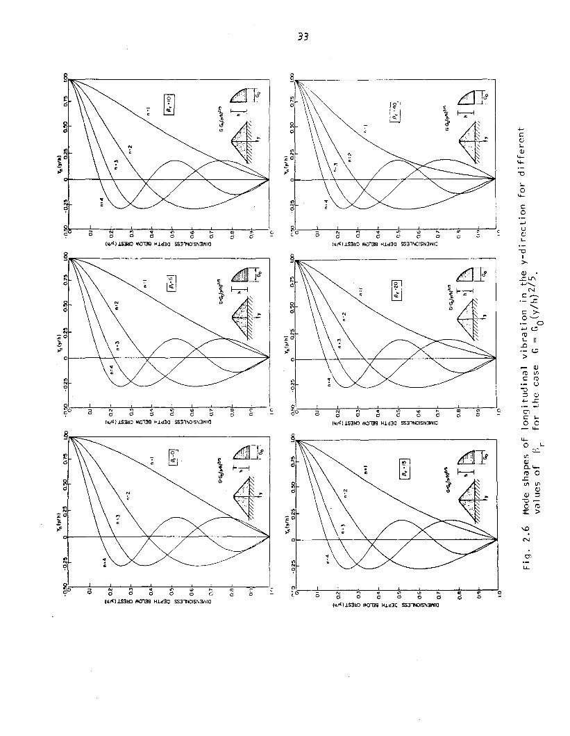
various cases of G(y) are shown in Fig. 2.4 through Fig. 2.7.
Another power series solution for Eq. (2.17) can be obtained by assuming
00
() \' k+sY Y = LakY
k=0(2.36)
In this case the indicial equation 2s = 0 has the repeated roots
sl = s2 = 0, yielding only one solution, and the resulting recurrence
relations are
~( 2 ~1 wh 2 2- -- --) - nEe" h a
4Eh2 vsO 0
(for k 2:. 2)
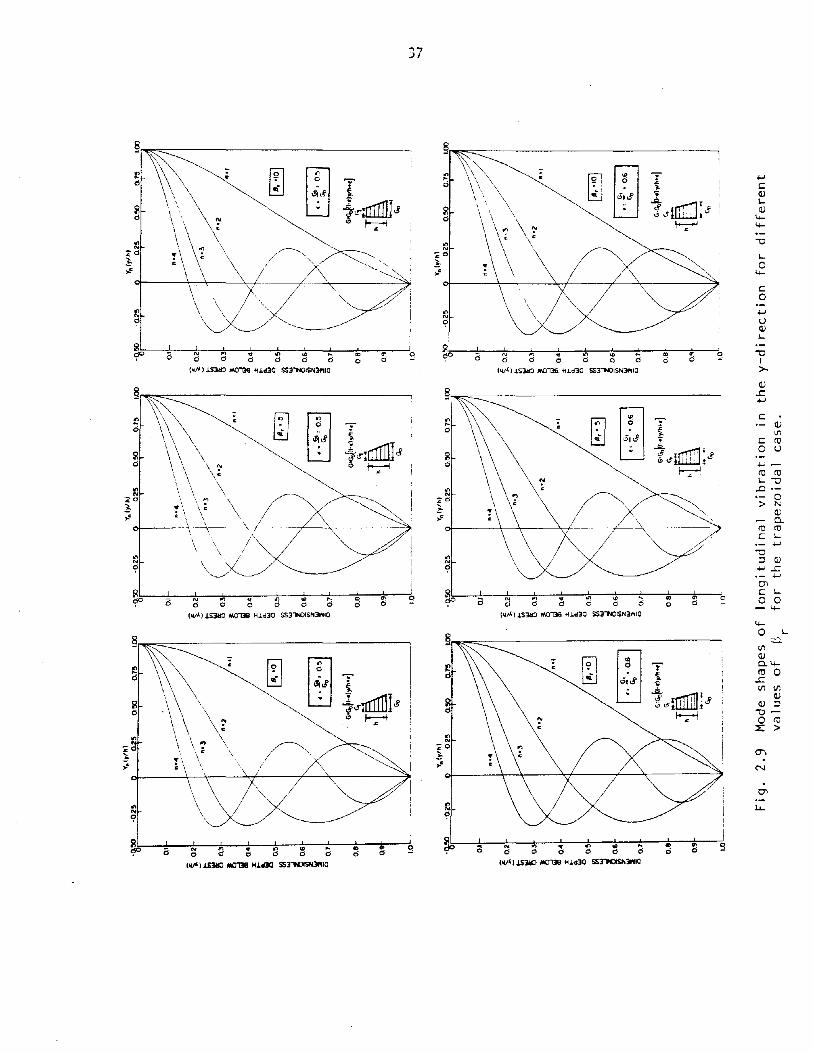
Like the case where G is constant, the solution of this trapezoidal
case (Eqs. 2.36 and 2.37) provides finite normal stress condition on the crest,
~'~
0z ¥ O. The roots w for different values of Sr for the trapezoidal
case are determined from the plots of the frequency equation in Figs. 2.8-a and
2.8-b. The mode shapes in the y-direction for this trapezoidal case are shown
in Fig. 2.9.
The frequency equation which defines the natural frequencies of vibration
can be written as
F(~,S ,S) = 0r
(2.38)

"fth/~I
"ftl
"hl
Yft,,~1
-~
00
2!l
o.!lO
0.7!
I1.
00-8
25
00
.25
0.50
0.7
51.
00-~
00
.25
o.!lO
0.7
51.
00
0.1
0.1
0.1
o.z
o.zo.z
:;;::;;:
~~
~
;:0
.3;:
0.3
·'3
;:0
.3
'"~
'"II!
wu
u~
oAl
/\/1
/~
~0.•
~~
0.•
-'E
19
ill1Il
.'III
~0
.5g0
.5j!:
0.5
Q.
Q.
~W
00
'""'
'":::
0.6
:::
0.6
f.30
.6-'
-'..
J
~~
z Q
!l10.
7~
0.7
~0.
7~
::E::E
Ii5
ais
0.8
~._hi
~"Go
('/h
'0
.80
.8
.~
~"~'''
''I1
.~)'G
OI'/
h)1
.;
,.,-
::
j,.
(.Go~
h'!:
:~~~:'
./\~
\,
/,
,0.9~
\\111
0.9
"-.
,1,
',.•
-."
~_,~.
0.9
,,
~I
'.
1.0'
r,
rJV
'I.
nJ
Yn
,y
/hl
V.I
,/h
)V
nl,
/h)
'-"
or·
.25
00
.25
05
00
.75
1.00
-8.25
00
.25
0.5
00.
751.
00-8
25
00
.25
0.5
00
.75
1.00
C~
0.1
[\
0.1rn
,(/
0.1
I~I~-~
/I
~
n-2
o:~
~f0
.2'
\J\
.I
/'
n~1
n'l
'"""
n::J
'",
~~
;:0.
3
G::3
;:0
.3
[ii,'2~
;::0
.3
'"'"
i0.•w
II!a:
uu
;l0.•
~0
.4
99
\V~
l!ll!l
~05
1~o!
~0
.5j!:
0.5
_.-
-.J
a.Q
.Q
.W
\oJ
lI/('
)(') '"
'"'"
:::
0.6
~0
.6~
0.6
..J
.....g
z
i0.7a
~I
t'$:""
''''~
0.7
~.
hi~)
'Gol
'/hl
~0.
7::;
i50
~I.'
\~"~"'
"a
ll,,
/,
h~
0.8
/)///
,j"
/'/',
h~
o,t
'Go
,Go
0.'
0.9
0.9
,r",
1.0
1.0
1.0
Fig
.2
.4M
ode
shap
eso
flo
ng
itu
din
alv
ibra
tio
nin
the
v-d
irecti
on
for
dif
fere
nt
val
up
so
ff,r
for
the
case
r.c
GO
(y/h
).

V.h
/MV
.ly
ll.1
Y.I
"Mo.z~
o.!lO
0."
LOO
-o.!lO
-oz~
1o.z~
o.!lO
0."
LOO
-a!l
O·o.z~
00.2~
o.!lO
OJ[
I
.'4~
r OJQ
.I
~0.
2!
o.z
!o.
z
~0.
~0.
3~
0.3
~~0
.4
n'l
~04
IIQ
4X
XX
l-
i0.51
AI
\/
1If,
./0
I..
l:i.. w
<>0
.5~
<>o.
!l
~III
IIIIII
w
~0
6
w...
J
50.
6~
0.6
V>z
~z
ww
::0;
~'"
00
.15
0.7
60
.7
G(y
)_G
o(yt
h)V
2G
IY)'
Go(
y/hl
"2
I\
II
AG
Iy).
Go(
yIhI
V'
\I
I1/
..t<W~
T~
0.8
~{t
.0
.80.
1If-
\I
IL
~I
O'T\l!
--'"l~--'''''~
I0.
90.
'9f-
1.0
1.0'
.,
1.0
Vn
(yth
lY
n(y
/h)
Vn
(y/h
)-0
.50
-0.2
50
0.2
50
.50
0.7
51.
00-0
.50
-0.2
50
0.2
50
.50
0.7
5~oo
-0.5
0-0
.25
00
.?5
0.5
00
.r5
~OO
~v
--
-N
0.1
0.1
0.1
{O
Z~
0.2
~0.
2t;;
0-
Ii;~
03
V> ...w
150.
3'"
~~
~0.
3
f\A
i/
rr4
~0
.4~
~m
0.4
en0
.4%
X
IIf,
'201
0-
X0
-0-
0-
W0
-0
-<>
0.5
......
o0
.5<>
IaIII
0.5
w...
III
~0
.6
w
50
.6~
06
V>
~Z
Z...
wi'5
0.1
:IE::0
;
G1y
).G
oly/
hl'"
00
.7o
0.7
Gly
l'G
o(yl
hlll
l
I\/
III
Gly
l'GoC
y/hl
lll
0.11
~{~
0.11
0.8
0.'9
.':'!.
.~-,..
0"
0.'9
0.'9
1.0
1.0
1.0'
Fig
.2.
5M
ode
shap
eso
flo
ng
itu
din
alv
alu
eso
fB
for
the
case
r
vib
rati
on
inlj
he
v-d
irecti
on
for
dif
fere
nt
G=
GO
(y/h
)2
.
Y.h
/MY
n(y
/hl
Y.l
r/h
l
l-0
.2!l
1nr~"
-05
0-0
.25
00.
2!l
O.!l
O0.
7!l
10
LOa
-O.!l
O-0
.25
00.
2!l
o.!
lO
0.11
-I
-----~
//
IO
J
~0
.2.-
4I
.·4
{0.
2~
02
~en
Ii;Ii;
."2
50.
35
0.3
S0.4
~;,:
~0
.4n=
10
xn
=1
~0
.4
0-
xX
Q.
0-
0-
...Q
.W
Q.
a0
.5!!
-C~
a0
.5[!f5
1:
0.5~~
I\
/~
l:ll:l
ww
~0
6~
06
w
'"~
zVi
.iii
0.6
...z
z::;
ww
:l;
6~.7
o0
.7:l
; o0
.7
0.8~
\/
IY
II
\!
IA
G'G
,,(yl
h)2J
O
--
0.8
0.8
O.'J
I-\
III
%'i
///7
.I'7
7?7
.?-
j--,
Io
.9f
0.9
'",n
I()
Yn
(y/h
lY
n(y
/hl
'n(y
/h)
-"""
0·0
25
00
.25
0.5
00
.75
too
-0.5
0'0
.25
00
.25
0.5
00
.75
1.00
0,
ii
i,
,~
0,
j1
II
-"S
O-0
.25
00
.25
0.5
0,
....or
II
II
-\.
t)
I----
---------
-------/'
/
W
0.1
~0.
1I
rz4
n=
4n
:4
~0
.2·
t0.
2""3
/.-
-rn
=.l
0-
0-
n=
2;:
'"'"
...w
'"V
1/
."2
~0.
35
0.3
w 5~
.-1~
n"f
~I
IA
I/
"'1
~0
4~
0.4
~0
4x
x0-
0-
X
Q.
Q.
0-
WW
~O.5
~(~l
jla
0.5
a~'~
~4~
l!£:
:'~
0.5
IIIl:l
...w
l:l
~0
6§
0.6
... J ~0
6z
~w
z:l
;w
00
.76
0. 7
:l; o
0.1
0.8
1-
\I
IG
'G"l
ylh
l/'
oJV
I/),"..
G'G,,(~)
'~,
II
.-.
T~
I0
.8/"-
Tf"
>.,
.
O.'J
I-\\
III
'//////.1
//////
II
I0
9r
'\Jj/
//////'1
:"u
,h;
JI
()~t
~I~
W/
/.y'/'
LJ1.
01.
0'"
Fig
.2
.6M
ode
shap
es
of
lon
git
ud
inal
vib
rati
on
inth
ey
-di
recti
on
for
dif
fere
nt
valu
es
of
r~fo
rth
ecase
G=
G O(y
/h)2
/5.
r

Y.l
y/h
)Y
.ly
/h)
Y.C
y/h)
-8.50
·0.2~
10
.25
0.5
00
.75
1.00
-85
0-0
.25
10
.25
0.5
00
.75
1.00
-0.5
0-0
.25
00
.25
0.5
0
oj
II
~o
j
I
I~
0
.·4
••
4O
J
02
0.2
i0.
2
""
~0.
3'
~~
;::0.
3;::
03
'"'"
........
~0.4
0:
0:
uu
~0
.4~
0.4
...J
...J
:J:
....III
I-ID
113"
51n.
~0
.5~
0.5
....n.
n.o
0.5
........
III.:>
0....
'"'"
§0.6
~0
.6~
0.6
...J
-'Z
Zz
....~
0.7
~0.
7~
~0
0.7
/\
/1V
G'G
oCy/h
)'"
()Ci
G'G
"CJ/
h)v
,
0.8
0.8
0.8
0.9
L~
I1
///////'i'-/////
II
I0
.90
.9
to1.
01.
0
Y.l
y/h
)Y
.(y
/hl
V.)
Y.(
y/h
I./;
::--O~
'0.2
50
0.2
50
.50
-0.5
0-0
.25
0.2
50
.50
-0.5
0-0
.25
00
.25
0.5
0
01
00
0.1
0.1
""
itI
"=
4
i0
2~
02
t0
.2
....
Ii;fi
t
~0.
3IS
03
~0.
3
~0.4
~0.4
~ g0
4
%:J
:
B:J
:
IA
I"'\
/r::
40
]l-
I-..
n.n.
fl....
....I""
151
00
. 50
o0
.50
.5
IIIIII
III....
....
i0.6i0.6
~0
6z
~....
!r::I
;
00
.70
0.7
a0
.7
G'G
olY
/h)V
>G
'Gol
y/h
lv,
I\
/I
II
G'G
olr
/hJv
,
o.s
f-\{
:/;~}~
0.8
-.,..
....0
.8
O.9
f-\\
.
I0.
91-
\\I
I/7
7/7
/71
T//
////
II
I0
.9
IY
'I
1.0
1.0
1.0
Fig
.2
.7M
ode
shap
eso
flo
ng
itu
din
alv
ibra
tio
nin
the
v-d
irecti
on
for
dif
fere
nt
val
ues
of
(3fo
rth
eca
seG
=G O
(y/h
)ll3
.r

35
0.50
f3r= /0
I 0.515 E = G1 =0 Go
0.25
OH-+--t--+-1'-f-----~~-------H+------~
-0.25
y
- D.SOOL.-----2..L5-----1SO-----7.LS----10..J.O-2-2---12J-S-----'150
DIMENSIONLESS FREQUENCY ~ = w hv2so
Fig. 2.8-a Plots of the frequency equations for the case where E = 0.5.

36
Q.5°n-rT------------------------..,
......-l3r= 10!4"i---- 5~_+_--- a
Y
G=Go~I-E) Y/h+E]G1
~m»m/.{~Go
OH---t-;--+-t'-+------\--"~-------hL.,L.---------t
0.25
-0.25
25 50 75 100II w2 h2
DIMENSIONLESS FREQUENCY W = 2Vso
125 150
Fig. 2.8-b Plots of the frequency equations for the case where £ = 0.6.
... ..,;)/
§
" ~ rnon
"~ tB
..~
i...0
~ c(I)
t~rrIIIJ]J~ .&. mrY ~
~. '! <5"1 ' . 1 J
I(I)\ .
~'~c:- O 4-. f-;-i ~ 4-
on on "'0N
£0 ~N
/ "- :;6 ~~ "-
~~
I ! 0~ " 4-
C
\ 0on on ....N
<;IN
<;I U(I)~
~ ~a N '" .. on OS> ... '" '" g <F a N '" .. on OS> ... '" tr g "'00 0 0 0 0 0 0 d 0 0 6 0 0 d c:i d I
W' 1.lS3lD MO"l3ll H~.30 SS3"'N01SN3I'liO 101' aS3lD MOUll H~.30 SS3"N:lISN3I'lIO >-
§(I)
..c~
" [J rnon
~ tB.. C
d .. ...~I~
(I)
t " " ~~~
V1
.;~~a1IllJ ~c ro
~ ~ ~ rrITIJT 0 U
6 " f-;-i 0 <; <5"1"1'" .... ~~ ro ro
~"'O
on on .0 .-N \ N
~6 \ ~o 0~ !\ ~ > N
~ ~(I)0-
ro roc l..~
;[on "'0N ::J (I)<;I .... ..c.- ~
I enI I I I
I~ C ~, , I I I
<F dN '" .. III OS> ... '" '" g <F a N '" .. on OS> ... '" '" g 0 0d d 6 0 d d ci d d d d 6 0 d ci d
- 4-W' 1.lS3lD MO"l3ll H~.30 SS3"'N01SN3"'O 101' 1.lS3lD MOUIl H~.30 SS3"'N01SN3I'liO
......0 ~
C2V1
~ rn ~ tB(I)
" "~IJ'
.. Cl. 4-
\ .. t ro 0
i1. IImr
..cl/l V1
t~nll1I1I~(I)
~
\\ ~ '! <5"1 i.j (I) ::J
0 \ 6l-;;-i "'0 -
\~~" t-;-t 0 ro
::E >on onN N
:;0 \ :;0
~ \" \ ~ "'"....." . '. \ ~
" N
en
:e on 1.L.
9 ~
~ ~a N '" .. on .. ... .. .. g a N '" .. on .. ... ..~ g
0 d d d 0 0 ci 0 0 d 6 6 6 6 ci
1111'1 J.SlIl:) M01lil H.l.d30 SSTHlfSN31'1I0 IIII' 1.lS1IO M01lil H~d30 SSTHlfSN3I'I1O

38
CHAPTER I I I
COMPARISON BETWEEN THE RESULTS OF THE PROPOSEDMODELS AND REAL OBSERVATIONS
I I 1-1. Earthquake Response Records
Resonant frequencies (in the longitudinal direction) of three earth dams
(Figs. 3.1, 3.2, and 3.3) in a seismically active area (Southern Cal ifornia)
are estimated from their earthquake records. Amplification spectra of the
dams' earthquake records were computed (see Refs. 1, 2, and 4) by dividing
Fourier amp1 itudes of acceleration of the crest records by those of the abut-
ment records (input ground motion) to indicate the resonant frequencies and
to estimate the r~lative contribution of different modes (see Figs. 3.1-c to
3.3-c). Then the two-dimensional models presented here were used to establish
from the observed fundamental frequency a value for the shear wave velocity,
or v 0'.swhich was then used to calculate other frequencies higher than
the fundamental. Each trapezoidal canyon of the three dams is represented by
an equivalent rectangle of length L equal to the average of the crest length
and the length of the base, e.g., for Brea Dam L = 0.5 (800 + 400) = 600 ft;
for Carbon Canyon Dam L = 0.5 (1,925 + 1,000) = 1462.5 ft and for Santa
Fe1 icia Dam L = 0.5 (1,275 + 450) = 912.5 ft. Tables 3.1, 3.2, and 3.3 show
comparisons between the observed resonant frequencies and estimated values
computed from the proposed analytical models; they also show the estimated
shear-wave velocities from the earthquake records.
From the comparison, the following observations can be made:
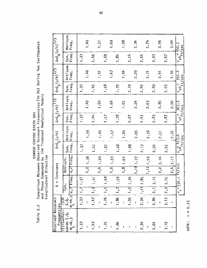
1. Observed resonant frequencies of Brea and Carbon Canyon Dams are in good
agreement with the symmetric modes' computed frequencies (from the models
in which the shear and elastic modu1 i of the dam material vary along the
d h .Q, 1 1 2) b d . h h . .ept , e.g., m=2 or 3 or 5 ut not as goo Wit t e antlsymmetrlc
modes' frequencies because the crest acce1erograph was located at the
crest mid-point of the two dams.

39
BREA DAM, CALIFORNIA
EMBANKMENT CROSS SECTION
DOWNSTR£AM
2' GRADED RIPRAP
(a) Cross-section of the dam.
(b) PIa n viewshowing locationof accelerographs.
Computed amplificationspectrum from the 1976earthquake (ML = 4.2)records.
AbutmentAccelerogroph
BREA DAM, CALIFORNIAl.l LOCATIONS OF STRONG-
o 200 MOTION ACCELEROGRAPHS'SCAL~ : II'
!D. OLIFtlliltR EFlUtIl.A(E eF ... 1 1916 (092D PST)
ftR 1lfIO, CR.IFftIR
flf'LlFlCRlI~ sPEtTlUl
'lEJ"ICA.. alPMHT
~l ...ft. T. [DIrETflVI'l
Fig. 3. 1 Brea Earth Dam.

CA
RB
ON
CA
NY
ON
DA
M.
CA
LIF
OR
NIA
EM
BA
NK
ME
NT
CR
OS
SS
EC
TIO
Nso
.C
Fl.J
F(R
tfA
EA
AT
tQA
(£fY
'•.A
I.I
1976
<09
20P
ST)
CRAD
ONC~YON
OA
H.
CFl
.fFM
N'R
FfF
'L1F
'CA
flO
NS
P[C
TfU
t
COf1
PnNE
:HT
PA
fR-l
El
TO(A
tA
XIS
<N50
N)
CRES
TM
,A,r
.A
IGn
ReU
TI'E
HT
UP
ST
RE
AM
RA
ND
OM
FIL
L
"FIL~E
RBL
A:K
E:"
,!~
--.-
-;.-
-.--
--A
PP
RO
XIM
AT
EE
XIS
TIN
GG
RO
UN
DS
UR
FA
CE
DO
WN
ST
RE
AM
~"
.,
5'
OF
EX
CA
VA
TIO
NA
CR
OS
SV
ALL
EY
FLO
OR
eoE
XIS
TIN
GC
HA
NN
EL
2'
STO
NE
e!.
5'
,-
FA
CIN
G1
103.
5'
TOE
PR
OTE
CTI
ON
-l6
"F
ILT
ER
BL
AN
KE
T
i- ~ ~ i·
-I="" o
8«'.
Cfl
.IF
rIIU
AE
Mna
JRK
EIF
....
.I
1976
<092
0PS
T)
Cf¥
II:IN
CFI
fflIrf
1R
f.C
A.IF
nNllI
A,",,-IFICATJ~
Sl'E
CT
fUt
Ctl
f'tl
£N
TI'f
lfR
..lE
LTO
OAH
mrs
(NS
Of)
CRES
TM
.R.T
.LE
FTA
llUTI
'EN
T
Com
pute
dam
plif
icati
on
spectr
afr
omth
e19
76ea
rth
qu
ake
(ML
=4
.2)
reco
rds.
(c)
i- ~ r i·
LE
FT
Ab
utm
en
tC
ru'
1.1
CA
RB
ON
CA
NY
ON
DA
M.
CA
LIF
LOC
AT
ION
SO
FS
TR
ON
G
MO
TIO
NA
CC
ELE
RO
GR
IIPH
S
Le
I!-
Ab
utm
en
t
~AcCele'Og'OPh
DO
WN
ST
RE
AM
Ho
rizo
nta
lq
II
I,5
?Oit
VtH
fico
',
II
,
o1
5"
Cro
ss-s
ecti
on
of
the
dam
.N \
N5
0W
"
SC
ALE
(a)
(b)
Pla
nvi
ewsh
owin
glo
cati
on
of
acce
lero
gra
ph
s.
Fig
.3
.2C
arbo
nC
anyo
nE
arth
Dam
.

..l;-
Fig
.3.
3G
ener
alvi
ewsh
owin
gth
eu
pst
ream
sid
eo
fS
anta
Feli
cia
Dam
and
part
of
the
spil
lway
at
the
rig
ht
(wes
tern
)ab
utm
ent.

42
SANTA FELICIA DAM
SANTA PAULA. CALIFORNIA
CROSS SECTION OF THE QAM
UPS1R£AM
2' OFDUMRIPRAP
DEVELOPED PROFILE ON AXIS DAM LOOKING UPSTREAM
IAXIS OF DAM
~ llOWMS'TREAhI
CREST DETAIL
Fig. 3.3-a Structural details of Santa Felicia Dam.
43
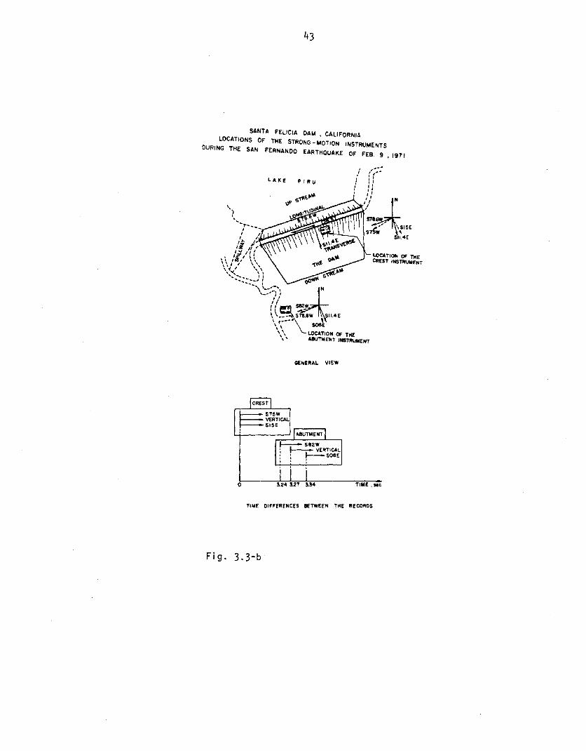
SANTA FELICIA DAM. CALIFORNIA
LOCATIONS OF THE STRONG - MOTION INSTRUMENTS
DURING THE SAN FERNANDO EARTHQUAKE OF FEB. 9 • 1971
LOCATION OF THECIlEST INSTIIVIoIENT
,.',,,
I,,
.--,","'-"l:"
/;~/~-::.,'I'f'n Ir S18 ,
_",' \SI5E
S7lIW 51~4E
PIIIULAKE
GENERAL VIEW
TIME ,MC
TIME DIFFERENCES BETWEEN THE RECORDS
Fig. 3.3-b

.o-
o- .~cn
a:a::z·OeD~3...:-u..--I.~Ula: .
If)
44
SAN FERNAND~ EARTHQUAKE FEB. 9. 1971SANTA FELICIA DAM. CALIFORNIAAMPLIFICATI~N SPECTRUMCOMPONENT ROTRTED PRRRLLEL TO DRM RXIS (S78.6W)
oLJ_..l--...-JL--..l.._...L---!L=!--~~::::::::""'~~~~-+---:::!----::!O. 1. 2. 3. 9. 10. 11. 12. 13. 1lL 15.
FREGlUENCY (HZ.)
o- .~tD
a:a:zo- .~.."
CU
U......-I.~::ra:
EARTHQUAKE ~F APRIL 8 1976 (0721 PST)SANTA FELICIA DAM, CRLIF~RNIA
F~URIER AMPLIFICATI~N SPECTRUMC~MP~NENT PRRRLLEL T~ DAM AXIS (S78.6W)
11. 12. 13. 1~. 15.FREQUENCY (HZ.)
Fig. 3.3-c Amplification spectrum of the 1971 and 1976 earthquakes.

Tab
le3.
1BR
EAEA
RTH
DAM
Com
pari
son
Bet
wee
nO
bser
ved
Res
onan
tF
req
uen
cies
(in
Hz)
and
Tho
seC
ompu
ted
byth
eP
ropo
sed
An
aly
tica
lM
odel
sW
hit
tier,
Cali
forn
iaE
arth
qu
ake
of
Jan
.1,
1976
(ML
=4.
2)L
on
git
ud
inal
Dir
ecti
on
Obs
.Res
.G
=co
nst
ant
G=G
O(y
/h)
G=G
(y/h
)1/
2G=
G(y
/h)2
/5G=
G(y
/h)
113
Fre
q.
a0
0(1
976
Ear
thq
uak
e)Sy
m.
Ant
isym
.Sy
m.
Ant
isym
.Sy
m.
Ant
isym
.Sy
m.
Ant
isym
.Sy
m.
Ant
isym
.M L=4
.2n
,rF
req
.n
,rF
req
.F
req
.F
req
.F
req
.F
req
.F
req
.F
req
.F
req
.F
req
.
2.75
1,1
2.75
2.75
2.75
2.75
2.75
-1,
23,
1.7
2.98
3.07
3.09
3.11
3.55
1,3
3.]!3
3.32
3.54
3.59
3.62
3.91
1,4
4.49
3.69
4.09
4.17
4.22
4.88
1,5
5.25
4.08
4.69
4.81
4.89
-1,
66.
074.
/ fS5.
305.
475.
58
5./ 15
2,1
6.17
4.93
5.53
5.64
5.70
-2,
26.
235.
075.
7b5.
815.
89
-2,
36.
555.
305.
976.
106.
17
-2,
1.6.
995.
616.
346.
506.
56
7.03
2,5
7.51
5.93
6.78
6.93
7.03
-2,
63.
106
.1.0
7.30
7.46
7.56
v=
656.
9ft
/sec
v0
=8/
1].
7vs
O=73
7.0
v sO=
71 9
.2v sO
=70
8.0
ss
ft/s
ec
ftls
ec
ft/s
ec
ft/s
ec
HaT
E:
The
Po
isso
n's
rati
o,
v,
of
the
dam
mat
eria
lw
asta
ken
tobe
0.11
0.
.t:
V1
CARB
ONCA
NYON
EART
HDA
MT
able
3.2
Com
pari
son
Bet
wee
nO
bse
rved
Res
on
ant
Fre
qu
enci
es(t
nH
z)D
uri
ng
Two
Ear
thq
uak
esan
dT
ho
seC
ompu
ted
byth
eP
rop
ose
dA
na1y
tic
a1
!1od
e1s
Lo
ng
itu
din
alD
irecti
on
~bserved
Res
on
ant
G=
Con
sta
nt
G=
GO
(y/h
)G=
G(y
/h)
1/2
G=G
(y/h
)2/5
G=G
(y/h
)I/3
Fre
qu
enc
ies
00
019
71S
anF
er-
1976
I
nan
do
LQ
.L
Q.
ISy
m.
An
tisy
m.
Sym
.A
ntis
ym.
Sym
.A
ntis
ym.
Sym
.A
ntis
ym.
Sym
.A
ntis
ym.
M L=6
.3M L=
4.2
n,r
Fre
q.
n,r
Fre
q.
Fre
q.
Fre
q.
Fre
q.
Fre
q.
Fre
q.
Fre
q.
Fre
q.
Fre
q.
1.3
71
.37
1,1
1.3
71
.37
1.37
11
.37
1.3
7,
I1
.40
1.4
01
.40
--
1,2
1.3
81
.39
1.'1
l1
.47
1,3
1.41
1.1
121.
'14
I1
.45
1.4
5
1,4
!-
-1
.44
1.4
6I
1.5
01
.51
1.5
1I
1.7
51
.76
1,5
1,I
.f31
.52
1.5
71
.58
1.5
9
--
1,6
1.5
31
.57
I1
.66
1.6
7I
1.6
9i
I1
.86
1.8
61
,71
.53
1.6
131
.78
;1
.79
1.8
2I
--
1,8
1.6
1 11
.30
:1
.92
1.9
41
.98
II
-1
.95
1,9
1.7
01
.88
2.0
7:
2.1
02
.14
!I
I
--
1,1
01.
77i
2.0
5I
2.2
42
.29
I2
.34
:i
2.3
02
.30
1,1
111
.85
2.
13I
2.4
3'
2.4
92
.55
I, I
,I
--
1,1
21
•~n
l2
.38
I2
.63
2.7
1:
2.7
9i
2.9
3!
2.6
42
.80
2,
13
.12
2.5
02
.83
2.8
9
--
2,2
3.P
I2
.51
2.8
52
.91
2.9
5
3.1
53
.15
2,3
3.1
52
.53
2.8
72
.93
2.9
7
--
2,4
3.1
712
•56
2.9
02
.96
3.0
0
v s=33
0• 1
ftls
ec
vsO
=4
13
.6v
sO=
36
3.3
v0
=3
55
.4v
0-3
50
.3ft
lsec
ft/s
ec
sft
lsec
sft
lsec
tJOTE
:\)
=0
.35
.t:
O'

SANT
AFE
LIC
IAEA
RTH
DAM
Tab
le3.
3C
ompa
riso
nB
etw
een
Ob
se
rve
dR
eson
ant
Fre
qu
enci
es(i
nH
z)D
urin
gTw
oE
arth
qu
akes
and
Tho
seC
ompu
ted
byth
eP
ropo
sed
An
aly
tica
lM
odel
sL
on
git
ud
inal
Dir
ecti
on
1971
G=
G(y
/h)Q
,/m19
76G
=G
(y/h
)QJm
Ear
thq
uak
eEa
rth
qu
ake
(ML=
6.3)
0(1
\=4.
7)0
Mod
eM
ode
Part
.O
rder
Q,Q,
Q,1
Q,2
9.-1
Part
.O
rder
Q,Q,
Q,1
Q,2
Q,1
Fact~
(n,r
)-=
0-=
1-
=-
-=
--=
-Fact~
(n,r
)-=
0-=
1-
=-
-=
--=
-F
req
.m
mm
2m
5m
3F
req
.m
rTim
2m
5m
3
1.35
1.00
1,1
1.35
1.35
1.35
1.35
1.35
1.27
1.00
1,1
1.27
1.27
1.27
1.27
1.27
1.70
0.61
1,2
1.79
1.60
1.69
1.71
1.72
1.66
0.67
1,2
1.68
1.50
1.59
1.61
1.62
1.86
0.62
1,3
2.34
1.89
?.
132.
172.
20I.
860.
731,
32.
201.
782.
002.
042.
072.
150.
442,
12.
772.
172.
582.
632.
652.
150.
382,
12.
602.
202.
432.
472.
502.
320.
621,
42.
942.
342.
592.
672.
722.
640.
381,
42.
772.
042.
442.
512.
572.
910.
532,
23.
002.
432.
792.
842.
87
0.91 l2,
22.
832.
282.
622.
672.
703.
150.
532,
33.
362.
513.
053.
153.
192,
33.
1G2.
372.
872.
973.
003.
490
.119
1,5
3.57
2.78
3.10
3.17
3.24
3.22
1,5
3.36
2.52
2.91
2.98
3.05
2,4
3.81
3.10
3.49
3.55
3.59
2,4
3.58
2.91
3.28
3.34
3.38
3.85
0.34
1,6
4.21
3.20
3.50
3.66
3.77
0.55{
1,6
3.96
2.56
3.29
3.44
3.54
3,1
4.26
3.35
3.87
3.96
4.02
3.71
3,1
4.01
3.16
3.65
3.73
3.78
11.0
30.
432,
511
.31
3.44
3.94
4.02
11.0
62,
54.
053.
233.
713.
783.
82
4.42
13,
24.
423.
484.
014.
104.
160.7
9{3,
24.
163.
273.
773.
863.
910.
363,
34.
633.
684.
234.
334.
394.
203,
34.
393.
463.
984.
074.
132,
64.
863.
764.
434.
524.
582,
64.
573.
534.
174.
254.
304.
880.
753,
45.
003
.91 1
4.52
4.62
4.69
4.59
0.44
3,4
4.70
3.71
4.25
4.35
4.41
vsO
(in
ft/s
ec.)
=7
22
.3967.~
827.
080
4.0
789.
5v
sO(i
nft
lsec.)
=61
:50.0
910.
577
8.0
756.
474
2.7
ap
art
icip
ati
on
facto
rw
aso
bta
ined
byd
ivid
ing
the
val
ue
of
the
ampl
itu
de
corr
esp
on
din
gto
ag
iven
reso
nan
tfr
equ
ency
byth
ela
rgest
amp
litu
de
that
corr
esp
on
ds
toth
efu
ndam
enta
lfr
equ
ency
.
NO
TE:
Bas
edon
the
in-s
itu
wav
e-v
elo
city
mea
sure
men
ts,
the
Po
isso
n's
rati
ow
asta
ken
tobe
0.45
.
4:
-.....J

48
2. Similarly, the comparison for the Santa Fel icia Dam (Table 3.3) suggests
R, 1 1 2 ,that the cases where m = 2' 3 and 5 are tne most appropriate represen-
tations for predicting the dynamic characteristics. Actually, from the soil-
stiffness determination (through the low-strain field-wave velocity measure-
ments on the dam (1,4) it was found that the 2/5-power variation law is best
resemb1 ing the measurements.
3. Average values of the shear-wave velocity for each of the three dams
were estimated by using their upstream-downstream earthquake responses
(Refs. 1,2, and 4) and existing shear-beam models (Refs. 9, 16, and 23) in
that direction. These values were: v = 677.0 ft/sec. for Brea Dam (as
zoned earthfil1 embankment constructed with a central impervious core
composed of graded material and two shells constructed of random material).
v = 375.7 ft/sec. for Carbon Canyon Dam (a random earthfi11 resting ons
100 ft of recent silt, sand and gravel), and vs 850.0 ft/sec. for
Santa Fel icia Dam (a random rolled-fill earth dam constructed from well-
graded alluvial materials consisting of clay, sands, gravel, and
boul ders) .
These values are consistent with those which resulted from the longi-
tudina1 models (Tables 3.1,3.2, and 3.3) in which both shear and axial
deformation were considered.
4. The nonuniform distribution of ground acceleration along the length of
the dam (as illustrated by the Fourier amplitude spectra of Carbon Canyon
Dam (Fig. 3.2-c and Ref. 2)) would considerably influence the nature of
the dynamic response of an earth dam to an earthquake. For instance, an
oblique angle of approach of travel ing seismic waves raises the possi-
bi1 ity of phase differences along the boundaries and the strong coup1 ing

49
between longitudinal and transverse vibrations. Obviously more precise
detailed evaluation of the seismic response of earth dams (e.g., via
a three-dimensional finite element or finite difference techniques)
is needed.
I I 1-2. Full Scale Dynamic Test Results
Results of full-scale dynamic tests on Santa Felicia Dam, involving
longitudinal forced vibration tests, Fig. 3.4-a,b,c (using only one shaker at
station E2 of Fig. 3.4-a) as well as ambient vibration tests, Fig. 3.5-a,b
(for more details see Ref. 3), were compared with those computed from the
suggested models. Table 3.4 summarizes these comparisons, while Fig.3.4-c shows
estimations of the measured modes along the crest (obtained during the
frequency sweeps); because only eight seismometers were used during the
longitudinal shaking, it was difficult to completely determine several modes
corresponding to the resonant frequencies of Table 3.4. The sol id lines con-
necting the data points of Fig. 3.4-c are estimates of the modal configurations,
while the dashed lines represent possible extrapolations; the local magni-
fication effect of the soil surrounding the shaker block is also shown. It
was found that some resonant longitudinal frequencies are very close (even
identical) to some of the upstream-downstream frequencies. This proximity
may suggest a strong coupl ing between these two horizontal directions, or
it may suggest that due to both the eccentricity of the single shaker (it
was not located on the longitudinal axis of the dam) and the fact that the
dam is not symmetrical, the upstream-downstream modes containing significant
longitudinal motions were excited. Again, the comparison suggests that
d 1 'th £ 1 1 2 t . . t h d .me e s WI m= 2 or 3 or 5 are mos approprIate to estlma e t e ynamlC
characteristics of the dam in the longitudinal direction. Furthermore,

UPSTREAM
50
DOWNSTREAM
CROSS-SECT ION
PLAN VIEW
UPSTREAM
o
P\RU
( If OUTLETP WORKS
300ft
DOWNSTREAM
Fig. 3.4-a Cross-section;plan view showing the measurement stations of thefull-scale dynamic tests on Santa Felicia Earth Dam.

51
3.000 3.500 ij.OOO ij.5oo 5.000 5.500 6.000 6.500 7.000 7.500 8.000FREQUENCY (HZ)
FORCED VIBRRTION TESTSON SRNTR FELICIR ERRTH-DRM
FREOUENCY RANGE FORCE (Ibs)
1.00 to 2.50 Hz 1609 (FREO.)2
2.00 to 3.00 Hz 1146
~ ::~~~22.50 to 5·00 Hz 3954.50 10 6.00 Hz 280 ( FRE~)
E1
LONGITUDINAL SHAKING
ONE SHRKER (E2)
~f\. STRT ION
t •t.
/ll
~/?~15/;'~
A tf ...
/ .•
0.500 1.000 1.500 2.000
00<:-00~0
00Ill!0
00r-;0
Wo00~"!~o--lCl.. o::1:0CI:~
00
l.LJ"'0-0-l'"CI:'::1: 0
cc~8
"!0
00~0
00
0
<:0
0.0
6.000 6.500 7.000 7.500 8.000
LONGITUDINAL SHAKING
FREOUENCY RANGE FORCE (lb.)
1.00 to 2.50 Hz 1609 (FREO.)2
2.00 to 3.002
Hz 1146 ( FREQ.)
2.50 to 5.00 Hz 395 (FRE>Jl4.50 10 6·00 ~:z 280 (FREO}
E1
( E2 )
STRTION
0.500 1.000 1.500 2.000 2.500 3.000 3.500 ij.oOO ij.500FREQUENCY (HZ)
FORCED VIBRRTION 'TESTSON
00<:-00~0
8Ill!0
00
N'":*0*
0Woa:: 0u.."!'-0WC>~o~o
-'"-l'Cl..
0
::I:CI: OClg!l.LJ •(/)0-~8::1:",a::'0 0z
00"!0
0
~.;
<:0
0.0
Fig. 3.4-b Response curves of longitudinal shaking.

FOR
CE
DV
IBR
AT
ION
TE
ST
SO
NS
AN
TA
FE
LIC
IAE
AR
TH
_D
AM
lON
GIT
UD
INA
LS
HA
KIN
G(O
NE
SH
AK
ER
)
FOR
CE
DV
IBR
AT
ION
TE
ST
SO
NS
AN
TA
FE
LIC
IAE
AR
TH
-D
AM
lON
GIT
UD
INA
LS
HA
KIN
G(O
NE
SH
AK
ER
)
.-""
,
10
0
~'-
--~f
=2.4
25Hz
l-__
I7_"
'-__~f
=1.4
25Hz
-----
_..r.v
-
$~
~':0
@I
-7'"
;'~",-:,
__:,f>
2.6
25
Hz
I'.~
__._f>
1.6
75
HZ
....../
......_
/I
•---_
_I·
Ul
N..
.
o@
~,0
0
--/-
',t;
A--
-Jf=
28
75
HZ
~~
i-;;
:;;;
:.<
l""-
-f>
L8
50
Hz
..._.
.....
'1
\..r.?
'--"'"
.---..
......_
.--
-70
,
-----."~
-;-
\;,:
_--
-f3
05
0H
Z~-
--.,
<,<
I-.
~--~f=1.950HZ
-_.I
~G>
,0~.
:~
0
/~
~~\
----
-,f=
31
50
Hr-
-.II
·"---
---1f =
21
55
H-_
..,)
'"I
l1i:
i!l'-
---
.Z
--
__
'-~
'---
.Z
---"
-,....
o'-
-o
.~
.....-~/~
..-\
r--
1~
-/-..
I~
1.-'"
....
I;.
'.
--
f=3
.23
0H
z---7'..
~--
f=2
27
5H
z\
II
\l~"-
-I
~I
7--
-.
""
'.
....-""
-..~
0
Fig
.3
.4-c
Est
imat
ion
of
the
reso
nat
ing
mod
eso
bta
ined
du
rin
gth
elo
ng
itu
din
alfr
equ
ency
swee
pson
San
taF
eli
cia
Dam
(on
lyon
esh
aker
was
use
d).

FOR
CED
VIB
RA
TIO
NT
EST
SO
NSA
NTA
FEL
ICIA
EA
RT
H-
DA
M
LO
NG
ITU
DIN
AL
"HA
KIN
G(O
NE
SH
AK
ER
)
FOR
CED
VIB
RA
TIO
NT
EST
SO
NSA
NTA
FEL
ICIA
EAR
TH-
DA
M
LO
NG
ITU
DIN
AL
SH
AK
ING
(ON
ES
HA
KE
R)
'""/
IW
We
I
r--"
./"1\
5t,
~.f=
4.3
70
Hz
'7
/,
__
.'--
@@
-,
I.
f
II
':
@e
i
-e~
_@'\
.---,
/@0"
"....<!.
4.7
00
Hz
t-
/_
I
,'--
I,./
I
,I
I@@
i.@
-@.<
!)--
--@
.......
,"'>\'
-@--
-".4
.87
5H
zk
7V
----
---"
"@
@
@e
l~/--
~'.3
.35
0Hz
'1-'{
1~-'.
\.,
~'\
r~
/~\
°_
....
.'_
0'
1-/@
---
.....'·
3.4
80
Hz
-.......
•7
-.....
..1
---
~,
,oI
'@'6
_0
G)
I10
°
ki
./0
....,_
f=3
.77
5H
z--@
I-~
'-~
••
0,.
\I
-./
@@
'-
'6,--""
~I6
@
\on
I.,.,
I.....
..-e.6\
__/f
)---
..,
f=4
.02
5H
z"
\.
,~
.,
°...
..-
/T
6 1,I
-,-
-61
6<3
.rel-
,,,,\,---:
,.4.175
Hz
~/
..I
.,
\~-.
/I.
\I
6'-
....
..I
.
f=5
.35
0H
z,_
.....
6°
Est
imat
ion
of
the
reso
nati
ng
mod
eso
bta
ined
du
rin
gth
e1
10
nq
itu
din
alfr
equ
ency
swee
pson
San
taF
eli
cia
Dam
,'
@e
Fig
.3.
4-c
(co
nt'
d)
--
....-..
....
I\~
I"
:Jf=
56
00
Hz
r\.
I\.
r...
'"•

..0
0....
WIH
D(
30
",,,
h,
SP
ILL
ING
OF
RU
IU,V
OIA
E1U
,atr
eem
_d
ow
n"r
••m
.-o
ol
•L
Dn
Vll
ud
'ne'
MO
Ot
,...
SA
NT
AF
EL
ICIA
EA
RT
HD
AM
AM
BIE
NT
VIB
RA
TIO
NT
E5
TS
Me
asu
rem
en
tS
tati
on
:E
4-0
5
Me
asu
rem
en
tD
ate
:3
-27
-19
78
Rec
orde
dM
otio
n:
l
2."
'MI'J
JfJ«
:T-
"l.
~::zw
~~~~
0:~-:.~
~Ir;~
-f\
II"lN
(\I
NN
<D
-""
~~
..:'" to ....
.." ..,.......
~ ~ l5 ~..~
~ i
rnU
p.'
ream
.do
wn
_"•
•,"
MO
DI
•L
Dn
vll
ud
lne'
MO
Ot
~~
~~g
"?-:-:"~"'!
u:(\
I~
ntr
ll""'\
"'[.0
00«:
:'-
",.
~~~;j;~
;Z~;;-,
\Of'
--r
:JO
\O_
nt.
n\J
J.........
_-
-N
(\1
C'l
nJ
N
SA
NT
AF
EL
ICIA
EA
RT
HD
AM
AM
BIE
NT
VIB
RA
TIO
NT
ES
TS
Me
asu
rem
en
tS
tati
on
:W
1
Me
asu
rem
en
tD
ate
:03
-15-
1978
Rec
orde
dM
otio
n:
l
"_
NO
WIN
D(
'0..
...
IS
Pil
liN
G0
'R
fSfI
WO
",
I...
.
D." D"Wl
I.:"
II
II
IJ.:;
'I
II
I1,
.:.,1
II
III
I,':
"I
II
II
II
5.r
o
....~ i IS ~
••'1
1 I
\J1
-l:'"
Fo
uri
eram
pli
tud
esp
ectr
ao
fth
elo
ng
itu
din
alm
otio
nre
cord
edat
dif
fere
nt
stati
on
son
dif
fere
nt
days
(th
efr
equ
ency
reso
luti
on
is0.
0073
Hz)
.
Fig
.3.
S-a
mU
ttetr•••.d
ow
na.
,••m
MO
OI
•L
on
gll
ud
lne'
MO
Ot
•.,
.LlI
NG
OF
JIlf
Sf.
,",O
'"
SA
NT
AF
EL
ICIA
EA
RT
HD
AM
AM
BIE
NT
VIB
RA
TIO
NT
E5
TS
Me
asu
rem
en
tS
tati
on
:W
5
Me
asu
rem
en
tD
ate
:03
-16-
1978
Rec
orde
dM
otio
n:
l
VI.
.,IT
lOO
NO
WIN
D(4
0..
...
)
..."'
'"<
1_
~t?~
O.a
DI
I;.
--
--
.'"['
I1\
1'"
f>J
I,
G.Q
O1
.00
2.0
0'.
IJJ
'4.(
'f'J
f.lJ
1KT
-H
l.
D.",or D'''
r~
.
i l5 ~..
"
<> w i

V1
V1
1.00
y
I''''I
IG
=Go
+H/L..fl
l.,ll-pL-+
-~"'~"""":
'~...•.~:.",:....~
.hI~
,-
y~
:-::":
:"f.:<
:'~~,
~.:...
.~
7,;
»»
£1
/);i
'r7
-'I
IIG
;;-t
SA
NT
AFE
UC
lAE
AR
TH
DA
M
Q41
I-
-I~
/1V
I/N
lIJ
t
Yn
b/h
)-0
.!50
-0.2
50
0.2
50.
!50
0.7
5O
.iii
ii'
ii'
Ii~
1.0
0.9
0.8
~0.
20.11
II
II
I:/"
I;M
~ ~ u0.
3
~ a:l :x:: ~ 0-
l&J a
G=
Go
(y/h
)0.
5t--t--~r-A~-+---~-I--+---+J'¥//--/-
~~~~~
l&J .,J
G:G
o(yl
h}21
5
~0.
6G
"Go
(y/h
)"3
~~~~~
oQ
7~=OS
IH
"M
---+
---~=
0.6
(1.1
)•
1,2)
EII, (1,4
)0
MO
DI
0.7
tI
Itn
II
I/I
!.,
II
II
Y n(Y
/h)
-0.!5
0-0
.25
00
.25
0.!5
00
.75
1.00
o'Iiii
iii
:a
0.8
JI
\\\\
I/1
11
IG
:Go(
ylh)
215
-+l-
----
.J-
I
Q9
rlI~
I/HI#~~;,W»~
{~ hJ
~I~
AM
BIE
NT
VIB
RA
TIO
NT
ES
TS
0.1
I"iJ
SA
NT
AF
EL
ICIA
EA
RT
HD
AM
",
YI
I!
1I
1.0
~ -J ~0.
6en z l&
J ::E o~0.2
1I
II
I,........-~I/
/jf
II
iQ3[j
L(~I/WI
I~ ~
Q41
I~A
II
le/w
"'-
II
:x:: ~ ~I
II
I1
aI
II'
llf
III
TIT
II0
.5n
o
Fig
.3
.5-b
Com
pari
son
betw
een
the
resu
lts
of
amb
ien
tv
ibra
tio
nte
sts
and
tho
seo
fth
ean
aly
tical
mo
del
s.

SANT
AFE
LIC
IAEA
RTH
DAM
Tab
le3
.4C
ompa
riso
nB
etw
een
Res
onan
tF
requ
enci
es(i
nH
z)Fr
omru
ll-S
cale
Dyn
amic
Tes
tsan
dT
hose
Com
pute
dby
the
Pro
pose
dA
nal
yti
cal
Mod
els
Lon
gitu
dina
lD
irec
tio
n
For
ced
Vib
rati
on
Tes
tsA
mbi
ent
'fib
rati
on
G=
G(y
/h)9
JmT
ests
Mod
e0
t1ea
sure
dM
ode
Des
igna
tion
and
Rem
arks
Ave
rage
Mea
sure
dO
rder
,Q,,Q,
,Q,1
,Q,2
,Q,1
Fre
quen
cyF
requ
ency
-=
0-
=1
-=
--
=-
-=
-n
,rm
mm
2m
5m
3
1 ./l2
511
1.11
461
,11.
446
1.44
61.
446
1.44
61.
446
1.67
5L2
:Id
enti
cal
toU
-Da
Mod
eSl~
1.63
8-
--
--
-1.
850
L3:
IIII
IIII
R1.
1.84
9-
--
--
-1.
950
L11:
II"
IIII
S2.
1.93
6-
--
--
-2.
155
L52.
175
I,2
1.91
2I .
711
1.81
31.
833
1•81
162.
275
L2.
317
I1,
32.
502
2.02
52.
278
2.32
62.
357
i2.
425
L2.
452
2,2
3.21
82.
694
2.98
73.
037
3.06
9
I2.
625
L6:
IIII
IIII
R3.
2.63
8I
--
--
--
2.87
5L7
2.88
01,
43.
148
2.32
52.
772
2.85
72.
911
3.05
0L8
:II
IIII
IIA
S3.
3.03
3-
--
--
-I
3.15
0L9
:II
IIII
IIR
4.3.
150
--
--
--
3.23
0L
3.22
91,
53.
821
2.59
83.
263
3.39
23.
476
3.35
0L1
03.
323
1 ,6
4.50
92.
846
3.73
73.
918
4.03
63.
480
L11
3.48
72
,33.
600
2.97
83.
319
3.37
73.
416
3.77
5L1
23.
775
2,5
4.61
53.
681
4.22
44.
303
4.35
311
.025
L4.
051
2,4
4.07
63.
323
3.74
03.
807
3.85
24.
175
L:
IIII
IIII
AS5
.11
.190
--
--
--
4.37
0L
13:
IIII
IIII
AR
3.4.
358
--
--
--
4.70
0L1
44.
667
2,6
5.19
94.
026
4.74
74.
843
4.90
14.
375
LIS
4.87
63
,45.
354
4.22
54.
843
4.95
25.
023
5.35
0L
-3
,55.
776
4.57
25.
223
5.33
75.
413
5.60
0L
-3,
65.
920
4.9
1 '95.
660
5.77
85.
857
vsO
(in
ftls
ee)=
774.
210
37.0
885.
88b
1.2
845.
6
~Upstream-Downstream
dir
ecti
on
.S
and
ASco
rres
pond
tosy
mm
etri
can
dan
tisy
mm
etri
csh
ear
mod
es,
whi
leR
and
ARco
rres
pond
tosy
mm
etri
can
dan
tisy
mm
etri
cro
ckin
gm
odes
(see
Ref
.3,
7,an
d8
).
\f1
0'

57
several modes of longitudinal vibration, along the depth, resulting from the
case of £/m = 2/5 are depicted in Fig. 3.S-b; the modal configurations
estimated from the ambient vibration measurements are also shown in the same
figure. The ambient-measurement results confirm the prediction by the
analytical models that for n = 1, the lower modes along the crest (low
values of r, e.g., r = 1,2) are associated with shear-type modal configur
ation along the depth, while the higher modes (large values of r, e.g.,
r ~ 3) are associated with bending-type modal configurations. This agree
ment between theory and observation may also be attributed to the fact that
relative to other earth dams in California, the Santa Felicia canyon has one
of the best-suited sections for an equivalent rectangle analysis, in the sense
that it is closer to a steepsided parallelograph than to a trapezoid. In
general, mode shapes (particularly configuration along the crest) of other
dams can be quite different from those of models due to irregular geometry
and zones of different materials. Finally, the first and second longitudinal
modes (1,1) and (2,1) along the depth (where n = 1 and 2), resulting from
all the proposed analytical models are also shown in Fig. 3.S-b; the modal
configurations estimated from the ambient vibration measurements are also
shown in the same figure. Again, the comparison suggests that model with
£/m = 2/5 is the most appropriate to estimate the dynamic properties of
the dam in the longitudinal direction.

58
CHAPTER IV
EARTHQUAKE-INDUCED LONGITUDINAL STRAINS AND STRESSESIN NONHOMOGENEOUS EARTH DAMS
IV-I. Earthquake Response Analysis
The two-dimensional model used in Chapter I I for finding the natural
frequencies and modes of longitudinal vibration of earth dams is util ized
for this earthquake response anal.ysis. The n~del which is a nonhomogeneous elastic
wedge of finite length (with symmetric triangular section) in a rectangular
canyon, resting on a rigid foundation, is subjected to uniform longitudinal
ground motion (acceleration) w (t)g
(Fig. 4.1).
To evaluate the magnitude and distribution of the modal strains and
stresses induced by earthquake motion, the equation of motion of the dam can
be written as
p ;2w + c dW _ lLIG(y) dW yJ - .!. LlnG(y) dW yJ = -pw (t)dt 2 3t y dY L dY Y dZL dZ g
(4. I )
where p is the uniform mass density of the dam material, w(y,z,t) is the
longitudinal vibrational displacement (relative to the base of the dam),
c is the damping coefficient, G(y) is the shear modulus (which varies along
the depth), and n[= E(y)/G(y) = 2(1 + v)] is an elastic constant (where E(y)
is the modulus of elasticity and v is the Poisson's ratio of the dam
mater i a I) •
A wide class of earth dams ranging from ones having constant elastic
modul i, I inear and trapezoidal variations of elastic moduli, to ones having
elastic modul i increasing as the one-half, one-third, two-fifths, and a
thgeneral (.Q,jm) powers of the depth are studied; i.e., the continuous variation
of soil stiffness is represented by the following suggested relationships for
both G(y) and E(y): (see Fig. 4.1 and Chapter II)
G(y) = G = constant (4.2-a)
G(y) (:LfJm [; = 1 1 2) (4.2-b)= GO h I '2"'3"'5

59
zz,w
LINEAR AND NONHOMOGENEOUSMATERIAL
y
I-RIGD BEDROCK
L.1
/
-Ib
y,v
b
r ~-_........._---_.. X,U
Ldy~-~
I.
The two-dimensional modelwith longitudinal groundacceleration
(a)
1.0
(b) Variation of stiffnessproperties along the 0./depth of the dam andthe results of the s:.
in-situ wave velocity~ 0.2
measurement on the t;;Santa Fel icia Earth Dam.
~ 0.3
~ 0.4wCD
X
t 0.5w0
(f)0.6(f)
w-oJ G:Go(y/h)~en 0.7zw~
0.8Ei e Wove Velocity
Measurements0.9
Santo Felicia Earth Dam
I.O""'"-------------~
Fig. 4.1 The model and the stiffness V~,!~:~ions considered in theearthquake response analysis.
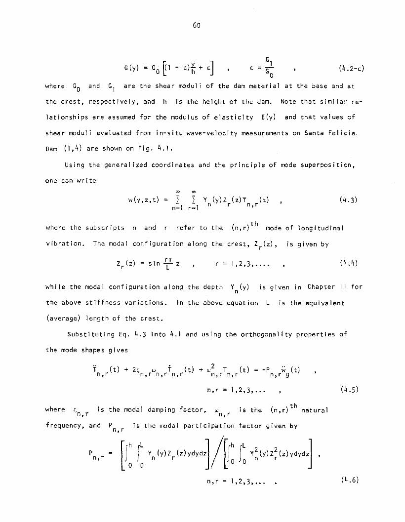
60
(4.2-c)
where GO and Gl are the shear moduli of the dam material at the base and at
the crest, respectively, and h is the height of the da~. Note that similar re-
lationships are assumed for the modulus of elasticity E(y) and that values of
shear moduli evaluated from in-situ wave-velocity measurements on Santa Fel icia
Dam (1,4) are shown on Fig. 4.1.
Using the general ized coordinates and the principle of mode superposition,
one can wr i te00 00
w(y,z,t) = I I Y (y)Z (z)T (t)n=l r=l n r n,r
where the subscripts nand r refer to the th(n,r) mode of longitudinal
vibration. The modal configuration along the crest, Z (z), is given byr
r = 1,2,3, .... (4.4)
while the modal configuration along the depth y (y)n
is given in Chapter II for
the above stiffness variations. In the above equation L is the equivalent
(average) length of the crest.
Substituting Eq. 4.3 into 4.1 and using the orthogonality properties of
the mode shapes gives
T (t) + 2r;: w t (t) + w2 T (t) = -P w (t)
n,r n,r n,r n,r n,r n,r n,r g
n,r = 1,2,3, ••• (4.5)
where is the modal damping factor, wn,r is the th(n,r) natural
frequency, and Pn,r is the modal participation factor given by
n,r = 1,2,3, ••• (4.6)

61
Because only the symmetrical modes can contribute to the response to
uniformly distributed ground motion, values of rare 1imited to odd integers.
Thus the participation factor becomes
4 ~':= - pnr n, r
n = 1,2,3, ... , r = 1,3,5, ... (4.7)
;'~
where P is the participation factor resulting from the modal configurationn,r
along the depth.
For the case where G is constant P is given byn,r
pn,r
4 2nl-J
l{;,)
n nn = 1,2,3, ••• r 1,3,5, ... (4.8)
where l- is theth
root of the Bessel function of the first kind andnn
zero orde r; J l is the Bessel function of the first kind and first order.
Values of ~ of Eq.4.7 are computed for different values of then,r
coefficient Sr[= n [rr~hr] for various cases of the stiffness variations (Eqs. 4.2-b
and4.2-c) and are listed in Table4.1.
The solution of Eq. 4.5 is obtained as a Duhamel integral in the form
T (t) = _---'-Pn'"';;:,r::::=::;~ [J tn, r .r."2 I 0
w r I - Sn,r n,r
Thus the problem has been reduced to that of the earthquake response of a
single-degree-of-freedom system. As the mode shapes and the modal participation
factor P are known, the normal stress and normal strain as well as shearn,r

Table 4.1
62
Participation Factors;'~
Pn,r
;', [I: [t]vn[tHt]J/[ ( [t]v~[tH~JJP =Mode n,r
f\=n [r~h) 2 Order(n , r) 1 2 1
G=G O[( l-E)t+ EJ
G=G O[t) G=Go[*) 2 G=G O[t) 5 G=G o[f) 3 E=0.5 E=0.6
(1 , r) 2.483 1.859 1.791 1.752 1.719 1.687
0(2,r) -3.332 -1 .650 -1.490 -1 .398 -1.295 -1.231(3,r) 4.005 1.539 1.340 1.230 1.068 1.006(4, r) -4.580 -1.466 -1 .244 -1 •124 -0.927 -0.870
(1 , r) 2.367 2.006 1.907 1.847 1.770 1.725
5(2, r) -3.999 -1.830 -1.623 -1 .505 -1 .357 -1.276(3, r) 4.481 \ .598 '1.377 1.256 \ .086 1. 0\8(4, r) -4.913 -1.502 -1 .268 -1 • 142 -0.936 -0.876
(l , r) 3.182 2.146 2.018 1.939 1.819 1.761
10(2, r) -4.613 -2.006 -1.755 -1 .610 -1.417 -1 .320
I(3, r) 4.990 1.660 1 .Lf 16 1.283 1.104 1.031(4, r) -5.272 :-1.539 -1 .292 -1.160 -0.946 -0.883
(1 , r) 3.421 2.275 2.122 2.027
15(2,r) -5.158 - 2. 174 -1.882 -1.712(3, r) 5.521 1.726 1.456 1·312(4, r) -5.656 -1 .577 -1.317 -1.178
( 1, r) 3.593 2.391 2.220 2. 111
20(2,r) -5.632 -2.333 -2.003 -1.811(3, r) 6.061 1.795 1.499 1.341(4, r) -6.064 -1 .615 -1 .340 -1. 196
(1 , r) 3.798 2.582 2.390 2.263
30(2, r) -6.390 -2.616 -2.227 -1.997(3, r) 7.124 1.943 1.589 1.404(4, r) -6.943 -1.694 -1 .391 -1 .231
(1 , r) 3.897 2.721 2.526 2.391
40(2, r) -6.932 -2.856 -2.424 -2.165(3, r) 8.101 2.100 1.687 1.472(4, r) -7.885 -1 .776 -1 .441 -1 .260

63
stress and shear strain modal participation factors can be computed and plotted;
in addition, the response spectrum can be used to evaluate maximum displace-
ment, strain and stress.
Using the modal solution (Eq. 4.3),the response of the dam to the earth-
quake longitudinal component can be written as
w(y,z,t) = I In=l r=1,3,5
yn(y)sin[nLTZ] Pn,r V (t)
V 2 I n,rwn,r 1 - sn,r
(4. 10)
where the funct ion V (t) is equa 1 to the quant i ty between the two bracketsn,r
in Eq. 4.9.
VI-2. Dynamic Shear Strains and Stresses
The magnitude and distribution of shear strains in the
are given by
th(n,r) mode
Y (y,z,t)n,r= _dW_ = __P_n;,=r==::::; _dY-,n-:-(_Y_) sin [_r_1T
L_z)
dY V 2 I dyw 1 - Sn,r n,r
V (t)n,r
n=I,2,3, ••• r = 1,3,5, ••• , (4.11)
or.~
4PY (y,z,t) = n~,~r;:::::.==~'¥ (Y...
h] sin [rnLZ
J1v (t)
n,r V 2 I n,r n,rrnhwn,r 1 - sn,r
n=1,2,3, ••• r = 1,3,5, ... , (4. 12)
where '¥ [Y...)n,r h is defined as it expresses the modal participation
and distribution of shear strain.
For the case where G is constant, the shear strain is given by
(4. 13)

For the cases where
is given by (see Chapter
64
G = G Lt) £./molh '
I I )
£.- =m the function
£. (g- 1)(1 --)
~ [y)a [2; _1] [*] m + a [~p] [*] + .••• + ak [*] m +
[ 2mI= k>T),(4.l4)n,r h
\",here a O =
a l = 0
aZ = 0
= 0
(4. 15)
a (k > 2mI- £ )
In the above equations vsO ( = IGO/p) is the shear wave velocity at the
base of the dam material; also, [2; - 1) and (2;) are integers.
The shear strain modal participation factors ~ or ~ (withn, r n
£. 1 110, 15, 20, and 40 and for cases of ; = 1'2'3'
through 4.5.lt is important to mention that the
n = 1,2,3,4 in the y-direction for values of sr[=n[r~hrJ equal to 0,5,
and t are shown in Figs. 4.2
linear case [~ = 1) gave
reasonable results for the natural frequencies and modes of vibration (Chapter I I I)
but gave erroneous results for the shear strain as indicated by the relatively
large finite values at the shear-strain-free crest and by the very low values in-
side the dam (Fig. 4.2). The occurrence of maximum values for shear strain at the
region near the crest is expected as the lower shear modulus near the top of the
dam would result in correspondingly higher shear strains for the same assumed

SH
EA
RS
TRA
INM
OD
AL
PA
RTI
CIP
ATI
ON
FAC
TOR
i'n
(y/h
lS
HE
AR
ST
RA
INM
OD
AL
PA
RT
ICIP
AT
ION
FAC
TOR
i'n
(y/h
)S
HE
AR
ST
RA
INM
OD
AL
PA
RT
ICIP
AT
ION
FA
CT
OR
'tn
lY/h
)
-25
5
~....
1~
.I.'A
't,·...
."h
__G
(Y):
Go
(y/h
l
:i1~
',~~
'/'
~~~
0.1.2
5
0.8 0.9
~0
.2
~ 50.
3
~ iii mQ
4x ~ a
0.5,
~ I04; B0
.7
~1~'~''''
09
~ "};.
0.2
0.1
n-4
0.8-2
5
~ 50
3
~Q4
x ~ 00
5
~ ~04
;
~ a0
.7
~J.
(::.
,"I
"'G
IYl-
Go
t"h
l,."
,:;,f:,
..';"
•.B
,"
.~
0.1
0.9
~ ... " ~0
.6
~ o0.
7
0.8
z ... ~0
.5
~0.
2
E 50
3
~ mQ
4
1.0
---------------J1
1I.1
---"
I..
I1.
0W
I'
SH
EA
RS
TR
AIN
MO
DA
LPARnCIP~TtoN
FA
CT
OR
"'"(
JIM
Ci'
\n
0'4
SH
EA
RS
TR
AIN
MO
DA
LP
AR
TlC
lPI'
T!O
NF
f\C
iC-(
·~·n(y/h)
-25
_1
00
~n.2'\:
n,'
IO
J
·'4
OJ
iQ
211
1,'2
0 1~Q
l~~
~Q3
IS0.
3\
V10
.3
JQ4JQ
4x
x l-t
IIIo
0.5
o0
.5III
III ...IQ4;
~0.
4;V
I
~ ::E0
0.7
B0
.1
~1~
I'GO
I'/h
)f~
-It":'>.
,..,-,
:.•.~~..
":.':
,.0
.8\-
.~
•.
'.'.
'h-1
0.8
/~.
.,":>
;1-"
0~Y
r"0
.90
."
1.0
1.0
"I~1-Got'/hl
Io;~
II',-ls
i
~.~
0.8O
J
no
"
0.9
,.
,1.
0...2!
J==
==c=
::u<
::::::
.I~
i\
95
}.,0.
2
~ 5Q
3
~ C}
Q4 . ... ~ n
O.~
g 1S0.
4;
'" ~ o0
.1
Fig
.4
.2S
hea
rst
rain
mod
alp
art
icip
ati
on
facto
rsfo
rth
ein
ear
case
.

0"
0'
[Pr":
~hr~
~--~~
,G
o
G('tl~Goly/hl!ll
,.o'
-l1.L
lL_
II'
"I
0'8t-+I~
-":~:5'~
::!?~t
\.h~
0.91
-,:
,I
Iy
t-G;i
~0.
2
St4E
AR
STR
AIN
tI.O
DA
LPA
RTI
CIP
ATI
ON
FAC
TOR
i'n1y
/h}
·10
-8-6
-4-2
0l
4r
iI~
:::::=
=-»
?i
r---
.---
-.-:
02 0.90.1 0.80,1
~ ~ f3 u ~0.
4
ill ~0.
5
'" ~0
.6
~ !l1 ~0.
7
5~ l50.
3 L. ;r; fu a
0.5
!:! oJ ~
06
~ o0.
7[P
EJ
Gly
)·G
oly,
,,)"1
•';~
..I~-
,.h
'',"
.h
-~.,
'~:.~.
'":~';;;'~"
:~-
",~
YG
o0
.90.8
;r; ~ 0
0. 5
~ ~0
6z '" "6
0.7
-.
SH
EA
RS
TR
AlN
WO
OA
LP
AR
TIC
IPA
TIO
NFA
CTO
R"'
nfy
/hl
"0
-6·6
~4
-20.
24
r'
i,
_::s:::r
:=::
::::
:=?
71I
SH
EA
"tS
TRA
INW
OD
AL
PA
RT
'C,P
,','l'
.)N
FA
crO
Ri'"
,(y/h
l
-10
-8-6
-4-7
02
4Iiii
~i
.::::C
==.-:
.-::=
z>?
I'
Ii
I
0.1
O.l
l-n
=4
~ l50
.3
'" ~0
4 1....)
11
\I
III
o."~•.•T~
M,,
;Y~'
;~\.
,1~
.,--G~
"}.
0.2
~Q
2
In !Ii0
3
SO.
~ o0
5
m ~0
6
~ "a0.
7I!
aG
fy).
Go
{y/h
lVIl
~":/
"\hl
-~~"'"
~,.
,..
t-G~
O.G
<·
0."
SH
EA
f;S
TR
AIN
'.~IJOAL
PA
RTI
CIP
ATI
ON
FAC
TOR
~'n(y/h)
10-8
-6·4
-20.
24
,'i
'...
!..-
-!-
-:>
=?
?I
Ii'
0.1
'-
0.9
SH
EA
RS
TRA
INM
OO
AL
PA
RTt
ClP
ATI
ON
fAC
TOR
't',,
(y/h
)
-lO-8
-6-.
-20.
2•
Iii
,:s
:x:
::::z
:w:;>
71iii
I
0.1
~0
.2
~ '" 1'50
3
S04
;r; >- 0- '" a
0.5
III '" g0
6in z '" " a
0.7
O.~
0.1
<'
t0
2"·
~ l50
.3
~ (I)
0."
x S I)
O.~)
E 6 ~ w :> i-i
0.' 1.0'
,!,
II
J1
.0'
III
"I
1.0
;I
"II
I
Fig
.4
.3S
hea
rst
rain
mou
alp
art
icip
ati
on
facto
rsfo
rth
esq
uar
ero
ot
case
.

10
'II
III
I
no
.O
J
SH
EA
RS
TR
AIN
MO
DA
LP
MT
ICIP
AT
ION
FAC
TOR
1'n
l"h
l-1
0-8
-6-.
-20
2•
Iii
i::::
:==::::
z::>?
ii
•i
f
~0.
2
Ii; !Ii0.
3 h1
/1,"
01
00
. 5III ~0
.6r
G°G
oly/
hl'"
~ i50.
7
0.8 0.9 1.0
G_G
o(y/
hl'lS
~
SH
EA
RS
TRA
INM
O(),
OL
PM
T'C
IPA
TIO
NFA
CTO
R"'
nl,
/hl
-10
-8-6
-4-2
02
•1I'~7i"fl
no•
0.1
~0.
2
~0
3
~0._
r I- 0-
W a0.
5III w 50
.6~ w :> 0
0.7 0.8 0.9 '_0
G·G
o(y
/h)V
S
I/I,~o
)
.0.O
J
0.8 0.9•
SH
EA
RS
TRA
INM
OD
Al.
PA
RTI
CIP
ATI
ON
FAC
TOR
....
I'/h
l
-10
-8-6
-.
-20
2•
iii
II
:S;:
::X
:::Y
>/I
i,
iI
r e; oo
.!)
~ ~6
Vio.
z w " o0
.7
{0.
2
In ~0.
3
~O.
(i' "
In~
0.3!
w is0.
3
"m
D..
g0_
[E
'5]
%r
t;:I-
W~
0.5
00.
5III
III...
~0.
6B0
6
~~ ~
a0
.75
0.7
0.8
0.8
0.9
0.9
1.0
1.0
G·~hW'h)tll
1/1"4
01
OJ~
n-4
SI1
EA
RS
TRA
INM
OD
AL.
PA
RTI
CIP
ATI
ON
fJ\C
TO
R'l'
n(y
/h)
-10
-8-6
-.
-20
2_
iii
':::r:
::::::
z:;:;Iii
ir
1.0 '
III
II
I
0.9
0.8
~0.
2
~0.3
mD
..
~ a0.
5III I::
~
G-Go
Cy/
h)V
S
'0.
OJ
SH
EA
RS
TR
AIN
MO
(),O
LP
AR
TIC
IPA
TIO
NFA
CTO
R".
Iy/h
)
-10
-8-6
-.
-20.
24
II
':::
:'::
::::
=»
71
""
~0.
2
OJ
SH
EA
RS
TR
AIN
MO
(),O
LP
MT
ICIP
AT
ION
FAC
TOR
".I
"h
)
-'0
-8-6
-.
-20
2•
Iii
ii':
::::
::::
Z::
;:S>
;i
',
ii
no
.
:< '}..
0.2
Fig
.40
4S
hea
rst
rain
mod
alp
art
icip
ati
on
facto
rsfo
rth
eo
ne-t
hir
dcase
o

n.,0.
1
SH
EA
RS
TRA
INM
OD
AL
PA
RTI
CiP
ATI
ON
fAC
TO
R"'
n(y
/h)
-10
-8-6
-.
-20
2•
1"'1~711'iir
0.2
... ~0.
3
~ ~O
'-' w m :r to:
0_5
w
IIpr
-1OI
0 ~0
6:l 0 VI ~
O'lG
<G"l
ylhJ
""
"'.+
-Ir.
.,
/hr
l0.
91-
,Go
to
G'o
,,(Y
1hJ"
"
B
SH
EA
RS
TRA
INM
OD
AL
PA
RTI
CIP
ATI
ON
fAC
TO
R"'
nh
o/h
)
-10
-8-6
-4-2
02
4IIii
i=::
::=:=-
:::::z
;>71iii
0.2OJ 0'81-+hI~
!"~"\"~-.':.:....~
,/
II
0.91
-J
~
n••
tOL
l'L
'LJI_
JJ"'
--_
_~
I;;0
3
~ ~o
'il: g
OS
o m ~0.
6
~ w0.
7g"...
G'o
,,(yl
h!""
~..•S
HE
AR
ST
RA
INM
OD
AL
PA
RT
ICIP
AT
ION
FA
CT
OR
t'n
(y/h
)
-10
-8-6
-.
-20
2•
111~;>Ji'
ii
0.\
nl
h :'"'
i·,·
I~1
1'--
{D.2
In ~0
3
~ III0
4
~ ~ l:l0
5
t illO
f,'
w '"o
0'
co
.-.
G'o
"'""
!,,,
,
Ifl,'4
01
II
"II
,1.
0
0.1
SH
EA
RS
TR
AIN
...a
OA
LP
AR
TIC
IPA
TIO
NF
AC
TO
R"t
n(y
/h)
-10
-8-6
-4-2
02
4i'~/'rii
I
..•0.
2
0.81
-+!
,."h
I~
.J;'
::"\
.,~
O.9~
;/~
,Go
~ l:I ~0
6
~ ~0.
1
~0.
3
~o.
'
~ ~0.
5
SHE
AR
STR
AIN
MO
OA
LPA
RTI
CIP
ATI
ON
FAC
TO
R".(
,/h
I
-'0
-8-6
-.
-20
2•
Ii
1:=::::
=:=::::
:::=>;Iii
ii
n"Q
J
02
~ m0.
3
~o.
'w m §
°lIfl"
201
l:I g0
6
ill ~0.
7
ol
.G'o
,,(yl
h!""
0.8+hI~
.j>
":;'
!'\"
=.
09
r'
/h-
l,
Go
1.0
G'o
"l,l
h!""
~ ~:I~
,Go
0.8
0.9
~O
.!t
02OJ
t;0.
3
5 ,. g0
4
SH
EA
RS
TR
AIN
MO
DA
LP
AR
TIC
IPA
TIO
NF
AC
TO
R't
'n(y
/h)
-10
-8-6
-.
-20
2•
rilli~>?lilil
II
II
"I
1.0
.. ... '~0
6
~ ~0.
7
"
Fig
.4
.5S
hea
rst
rain
mod
alp
art
icip
ati
on
facto
rsfo
rth
etw
o-f
ifth
sca
se.

69
R, 1 1 2shear stress. Cases of m= 2' 3' and 5 gave similar results for
the distribution of shear strains within the dam. The coefficient S dependsr
on the Poisson's ratio v of the dam material, the dam's depth-to-length
ratio (h/L), and the order, r, of the modal configuration along the longi-
tudinal axis of the dam (low Sr(= 0,5) implies low modal order (r = 1 to 3)
or a very long dam, while higher values of Sr(> 5) indicate a short, high
dam or higher modes along the crest). The basic characteristics of the shear
strain modal participation functions, '¥ ,n
(i.e., the maximum values and
their locations and the relative modal contributions) can be easily extracted
for various types of dams from Figs. 4.2, 4.3, 4,11, and 4.5.
For the case where G = GO [( 1 - £) [*J + EJ,given by
the function '¥ ('i...)n,r h is
ak= - k;O [k(k - I) 0 - £)] ak_1+ [[w~~:T no [r~hJ 2}k-2
- [nO - £) [r~hrJ.k-3 k~ 3
w ['i...\ [ ) [ 12[ ]'k-
n. n, r hJ = 2a 2 t + 3a
3 tJ + .•.. + kak * + •••.
where aO =
a l 0
a2 = -410 [[w~::hr-no ir~hr]
k > 3 , (4. 16)
(4.17)
This function is shown in Fig. 4.6 for the two cases (= 0.5 and 0.6 and
the different values of S = 0, 5, and 10.r
In general, Figs. 4.2 through 4.6 show significant contributions from higher
modes along the depth (n ~ 2).

......
o
__J
~~J
III,
"0
1
r..~.
0.5\
I··t·0
6\
G<J~
'I""
")
hl~
.......... Go
G:~~I"I
YIh+']
-I~
"'-
--t
Go
.'4
SHE
AR
STR
AIN
MO
DA
LPM
TlC
IPA
TIO
NFA
CTO
R"'
.Iy
thl
~l0"
,1
1.0~_·
0.8 0.9 1.0
·'
SHE
AR
STR
AIN
MO
DA
l.PA
RTI
CIP
ATI
ON
FAC
TOR
"'.I
,th
)I
,~
~~
~
Or-
-:::
:;;:;i
ijiiI
._-~------,
0.9O.e
i0
2
t; ~0
3
~ ~0
4% .... e; a
0.5
~ ~0
.6~ ~ o
0.1
~0
2
t; ~0
3
i04 % lL ... 00
. 5~ ~
0.6
'" ~ 00
.1
~
~a
~FI")yIh")
Gt
hI~
Io--
-ol
Go
G~~I'fIY/h"]
G,
-I~
o.-
iGo
.'4
SHE
AR
STR
AIN
MO
DA
LPA
RTI
CIP
ATI
ON
FAC
TOR
"'.l
yth
)
~I
SHE
AR
STR
AIN
MO
DA
LPA
RTI
CIP
ATI
ON
FAC
TOR
"'.l
yth
)
(»,.1
Or
c.e 1.0
0.91.0
,~
0.9o.e
i0
2
t; ~0
3
~ ~0
4% ~ o
0.5
~ ~0
6~ ~ o
0.1
i0.
2
t; ~0
3
~ ~0
4% .... e; a
o.!!
i~ ~
06
~ , o0.
1
~~ I..<to
0·!!
1
Go<1
J~'h
"h")
hI~ Go
Go<J
'-'I""
,..)
hI~
"'-
iGo
&'SH
EA
RST
RA
INM
OD
AL
PAR
TIC
IPA
TIO
NFA
CTO
R't
.ly
th)
1.0
o.eo.e
0.91
I
0'"
OJ
0.9,
SHE
AR
STR
AltI
MO
DA
LPM
TIC
IPA
TIO
NFA
CTO
R't
.ly
thl
II
0"
&
•.OL....._~-
i0
2
~0
3
i04
% .... ~o.
!! i06 ~ IS0.
7
t· g03
i04
% lL l!:O
!! i06 , IS0
.7
Fig
.4.
6S
hea
rst
rain
mod
alp
art
icip
ati
on
facto
rsfo
rth
etr
un
cate
dca
se(w
ith
£=
0.5
and
0.6
).

71
NO\'J, the modal shear stresses are given by
T (y,z,t) = G(y)y (y,z,t).n,r n,r
(4. 18)
For the case where G is constant, multiply the numerator and denominator
of Eq. 4. 13 by wn,r which is given by (Chapter I I)
(4.19)
and then Eq. 4. 18 becomes
(4.20 )
In Eq. 4. 19 is the shear wave velocity.
It follows that the modal participation and distribution functions for
the shear stress are expressed by the function J 1 [An *J as in the case of the
shear strain (Eq. 4.13).
The modal shear stresses for the case where G(y) = Go[*fJmare given
(using Eqs. 4.11,4.12, and 4.18) by.'.
4Gi [J [ JT ( Y, z , t) = :o-n:.,=r=:;::::; 4> 1.h
sin r7LrL V (t)
n,r V 2 I n,r n,rrrrhw 1 - r;;n rn,r ,
(4.21)
where ¢ r1.h) is defined byn,r\.
it expresses the modal
participation and distribution of shear stress, and it is given by
• • •. + r~ (k+ 1) - ~
a [1. +k h
(4.22)

n =
where the a's coefficients are defined through Eq. 4.15.
The shear stress modal participation factors ~n,r or ¢n[*) (with
.£ 1 1 21,2,3,4) for - = 1,-,- and - are shown in Figs. 4.7 through 4.10.m 235
For the linear case [~ = 1) the shear stress distribution (Fig. 4.7) seems
physically more reasonable than the shear strain distribution shown in Fig. 4.2.
Like the shear strain case, great similarity exists among the cases of
!. = 1.. 1.. and 2m 2' 3 5
The fun ct ion
of the shear stress distributions.
¢l [:t.1 for the linea r truncated s t i ffness case (Eq. 4. 2-c)n, r h}
can be expressed, in terms of 'if of Eq. 4.16, asn,r
~ [:t.J = r( I - d [y.) + EJ 'f [y.\n,r h ~ h n,r hJ(4.23)
The shear stress modal participation function (~n,r or ~n) is plotted in
Fig. 4. I I for the two cases where E = 0.5 and 0.6; for each case four modes
(n = 1,2,3,4) are shown for the values of 6 = a 5 and 10. Again, the basicr '
features and differences of all the above-mentioned stiffness variations for
the shear stress case can be easily deduced from Figs. 4.7,4.8,4.9,4.10, and
4. 11.
IV-3 Dynamic Axial (Morna]) Strains and Stresses
Analogous to the development of the previous equations expressing dynamic
shear strains and stresses, the magnitude and distribution of normal (axial)
strains and stresses in the th(n,r) mode can be given by
and
a (y,z,t) = E(y}t: (y,z,t) = T)G(Y)~wzn,r n,r 0
(4.24)
(4.25)

!IH
[M5T
IlES
SllO
DA
L~IC_~
FAC
TOR
.,,(
,/h
)S
HE
AR
ST
RE
SS
MO
DA
LP
MT
1CIP
AT
ION
FA
CT
OR
4»n(
y/tl
JSH
EA
RS
TR
ES
SM
OD
AL
PM
TlC
1MT
lON
FAC
TO
R••
(,Ih
)
SH
E'"
ST
RE
SS
MlO
AL
~1C1PllT1lJN
FAC
TO
R.,,(
,/hl
'-J
...."S
HE
AR
STR
ES
SM
OD
AL
PA
RT
ICIA
\TK
lNFA
CTO
R4»
n(yl
h)
-0.2
50
0.2
50
.50
I~;.>
I~l~l"GO("h)
I
~Go~
02
0.9 1.0
II
,I
hI
0.8
£ ~ ~0.
3
0:
V fA ~0
.5
~. '" f3
0.6
g ~0.
1
B
0.9
SH
E'"
ST
RE
SS
MO
OA
LP
llRTI
CI..
..TIO
NFA
CT
OR
.,,(
,/h
l
-0.5
0-0
.25
00
.25
0.5
0
°1~j?1
J~GI
:I
til~)::Go(Y/")
~~
0.8 1.0
I\I
Ir
I,
t I-0.
3
~ v m0
.4
~0.
5
~ ::l w0
.6-' z Q 8
01
:> C3
0.5
00
.2'
1~)O
GOI"
hl
h~
o-0
.2'
£ ~ ....0
.3
~ ~0
4
ill ~D
.!
o '" ~0
.•,
~ ~0.
1:> is
0.1
0.5
0
I
[T~
0.2!
»
"::
4
o-0
.25
.,1
o:~
08
02
£ ~ ~0
.3
v ~0.
4
g ~0
5
~ '" ~0
.6
~ ~0
7:> "
II
II(
II
10
a
0.2
5o
0.9
0.8 1.
0'I
II
III
£ ~ f3 ~O
A
~ ~0
.5
o '" ~0.
6
g !lI ~0.
1
is
oo.s
o-0.2~
00
.25
0.50
I__
--::..:
::J0
0>
;>I
Of~~('
Ih 1g;:
':cG
o(J
/hl
~
0.8 0.'
02 LO
II
II
II
.....0
.3'0 il! v ~
0.4
" g "0
5~ '" t::
0.6
g f0.1
Fig
.4
.7S
hea
rstr
ess
mod
alp
art
icip
ati
on
facto
rsfo
rth
ein
ear
case
.
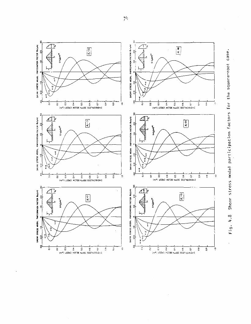
!!
I'"
ILf
)
'.I
[;;;
~OJ
'.0
0.80.1
02
SH
EA
RS
TR
ES
SM
OD
AL
PtlR
TIC
IP'A
TlQ
NFA
CTO
R~n(y/hl
'3.0
'2.0
-1.0
a1.
02
.03
0I
ji:
=::
::;;
:;0
!Ji7iii
0.9
t;0
.3w a: u ~
0.4
ill ~0
.5
o '" ~0
.6-' z o i2 ~
0.7
i5
~51
G'G
J,yl
h),1
2
SH
EA
RS
TRE
SS
t.100
AL
PA
RTI
CIP
ATI
ON
FA
CT
OR
~n(y/h)
-'.0
-2.0
-1.0
01.
02
.03.
0I
,1
::=
:;:;
tIi!
!ii)
iI
I
0.8
II
II
II
I1.
0
020.1
0.9
E0.
3
[5 ,.O
Ag ill ~
05
w o '" ~0
.6-' z Q 15
0.7
"i)
a
G'rj
<Jy
lhl'"
02
SHE
AR
ST
R£S
SJo
IOO
AL
PIl
IIT
'CR
TIO
NFA
CTO
Re.I
,lo
l
-3.0
-2.0
-'.0
01.
02
.03
0i
ii~iii
0.1
O.A
0.9
c }. ~
0.3
w 5 =:0
4g ill ~
05
w n '" ~0
6_. '"o o0
.7
II
II
II
!to
IIJ'
~J
G'rj
<Jy
Ih)'"
SH
EA
RS
TRE
SS
MO
DA
LP
MT
ICIP
AT
tON
FI\C
TOR
~dy/hl
II"
II
,I(
J
O~
02
Ol~·3
.p-2
i O-1
.,0-=
--?'iO
2?
','"
.[
.......
I'--
O.'~
,·n
•./'
/'
II
_.L
,.,.
,.U
--"'~"-LJ
~$h:~~~~'l~
ICo
c }. ~
0.3
u r4
~0
5
l'J '" :fl0
.6oj 9 ~
0.7
;; ,;
111 "2 °1
G>r
j<Jy
Ih)V
Z
SH
EA
RS
TR
ES
SM
OD
AL
PA
RTI
CIP
ATI
ON
FAC
TOR
~n{y/h)
-2.0
-1.0
n1.
02
.03,
0I
I::
;;:!
i¥i
i
0.1
02'3
.0
OR
09
c }. ~
0.3
a: u rA
g05
o '" :fl0.
6-' z Q ~
0.7
:> 5
1.0
ILL
'--',-
-','-
---'
,.-1
...,-
------'
o
SH
EA
RS
TR
ES
SM
OD
AL
PA
RTI
CIP
ATI
ON
FA
CT
OR
~n(y/h)
-2.0
·1.0
01.
02
.03.
0
'~
"1
07
O.R0.
'
}.
'3.0
0.9
::nO
."i
~ ~0
4
~0
'
W '" ~0
6
;) ~0.
7,;
Fig
.4.
8S
hea
rstr
ess
mod
alp
art
icip
ati
on
facto
rsfo
rth
esq
uare
-ro
ot
case
.

..~ \h
[i~.,
G:G
o(y/
hl'I
S
G1I
Go{
y/hl
tlJ
-I~
~l'lm"fifi;;;~l-J
0.8 0.9 1.0'
II
II
I
SHEA
RST
RE
SSM
OD
AL
PMTI
CIP
ATI
ON
FAC
TOR
t~n(
y/hl
-2.0
02
0
SHEA
RST
RE
SSM
OO
AL
PM
nClM
TIO
NFA
CTO
R~(,lhl
-2.0
02
.0
1.0
'I
II
I'
I
~ ~0.
2
~0.
3
I04
~ o0.
5III a0
6~ ~ o
0.7
0.8 0.9
{0.
2
~Q31
a04
~ 00.
5III L6 ~ B
0.7
EJ
/-"
201
G"G
o(y
/h'V
]
G°c
;,,(lO
Ih,II
S
0.9 1.0
'I
II
II
I
SHEA
RST
RE
SSM
OD
AL
PAR
TIC
IMTI
ON
FAC
TOR
~n(,'hl
-2.0
02.
0
0.8
SH
EM
STR
ESS
MO
DA
LIW
l'1lC
1MTI
ON
FAC
TOR~1,'hJ
2.0
~Q
2
~O
l
a04
~ o0
.5III L6 ~ B
0.7
~0
.2
~0.
3
I04
% .... l:J
aI
00
.5III ... 50
6!e w "o
0.7
0.8 0.9 I.n
~
G·G
oly/
hl":
J
G°c
;"h
/h)I
IS
2.0
o-2
.0
t; ~
SHEA
RST
RE
SSI«
JOA
LIW
l'1lC
1MTl
ON
FAC
TOR~(,/h1
0.9
0.8 I.n
'I
II
II
.J
0.8
SHEA
RST
RE
SSM
OO
AL
PAR
TIC
IMTI
ON
FAC
TOR
~n(
,Ih
)
-~O
0~O
o.~
II
II
II
I1.
0
~0
.2
~0
.2
t; ~O
l,. ~
04
% S o0
.5
III g0,6
~ ~ o0
.7
III ... ~ ~0
.62
' ... "o0
.7
Fig
o4.
9S
hea
rstr
ess
mod
alp
art
icip
ati
on
facto
rsfo
rth
eo
ne-t
hir
dcase
.
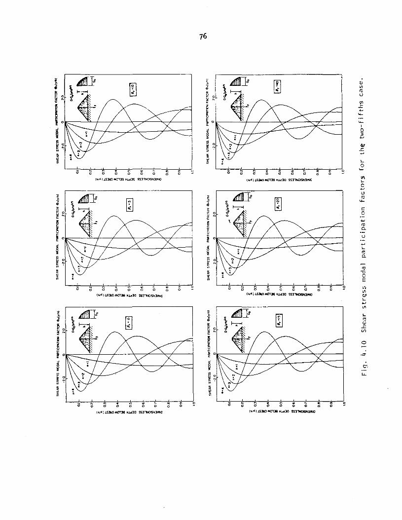
II
II
II
I1.
0
~
1II"~1
'·,·,°1
G'G"
l\Ollll
'"
0.2
II
II
II
II.e
SH
UR
ST
ll£S
SM
OD
AL
PMT1
ClI'
llTO
tFA
CTO
R"1
,11
1'
-2.0
02.
0
II
II
'I
,1.
0
OJ
OJ
SH
EA
RS
TRE
SS
MO
DA
LP
M'T
ICfP
I,TK
NFA
CTO
R~"(.,./hJ
'2.0
02
0
09
02
0.8
~ ~0
3
~ ~O~
g ~0.
5~ m
06
g ~0
7:lE is
0.8 09
t;0
3
~ ~O~
g ~0
5l'ji ~
06 i07 i
III,'20
\
~
G'Go
I\Ollll
'"
0.2
0.9
0.8
~ iii0
3
~ ~0
.'
ill ~0
.5~ ~ i06 i0
.70.1
SH
EA
RS
TRE
SS
MO
DA
LP
llRTI
CIP
lIlTK
JNfA
CT
OR
ttn
(y/h
)
-2.0
02
0
1.0'
II
I!
I
II
'I
II
,1.
0
SH
EA
RS
TRE
SS
MO
DA
LP
/lRTI
ClP
ATI
QN
FAC
TOR
tt"l
y/h
l
0.2 O'
OJ
0.8
~ ~0.
3
~ ~a.
il! ~0
5
~ m0
6
g ill0
.1... :lE is
BB
G~(\OIlII'"
.I~
,'h
-1,
Go
0.8 0.9
0.2
sttE
AR
STR
ES
SM
OD
AL
PA
RTI
CIP
ATI
ON
fAC
TO
Rtt
nly
/h)
-2.0
02
.0
0.9OJ OJ
0.8
Sttt
::AR
StR
ES
SM
OD
AL
PMnC
IMT
ION
FACT
OR
ttn
(y/h
'
-20
02.
0
02
II
II"
I1.
0
~ t;0
3
~ ~O~
ill ~O~
o ~ ~0
3
~ ~O~
ill ~O~
i!j ~0
6 i07 i~ i06 w0.
7:lE is
Fig
.4
.10
Sh
ear
stre
ssm
odal
part
icip
ati
on
facto
rsfo
rth
etw
o-f
ifth
scase
.

""', ')
~~.),..,...)
G,
hl~ ..........
.Go \' )~
,~
..t'''1
1.0
SH
iAR
ST
RE
SS
MO
OA
LfM
TlC
IPA
TlO
NF
AC
TO
R..
",/
hl
Ja
0,
:::::1
M'
i
OJ
0.8 0.9
~0
.2
Ii; ~0
3
g lil0
"% lL l':
O.~
!a ~0
6
~ 00
.1
~
c;.c
J~'1
""''
'1G,
hl~ ..........
.Go
0.9
SH
EA
RS
TR
ES
SM
OD
AL
PtlR
1"IC
IPA
TlQ
NFA
CTO
R~n
(,/h
I
Ja
0,
,~
0.8OJ
1.0
~0
2
Ii; ~0.
3
g lil0
"~ ~
O,~III ~
0.6
~ ~ Ci
0.1
~
c;.c
J~·)
""''
'1
hl~
'"--
--4
Go
I.O
L----l-
L-_
0.8OJ
QCJ
I
SH
EA
RS
TR
ES
SM
OD
AL
JMT
ICIP
AT
IO'l
FAC
TOR
..,(
,/h
)I
rr-a
Ii
::::::ii
iiM
~0
2
Ii; ~0
3
g lil0
"% lL l':
o.~
III i06 ~ 50.
1
'-J
'..J
) [~~
)G<tJI
.•I""'
..)
'l~
~..
Go
((
SH
EA
RS
TR
ES
SM
OO
.Il.
IMT
ICF
IIT
IOIl
FAC
TOR
"'1
,,,)
J~
0'
•--
---
0.8 1.
0
09
Ii; ~0
3
g lil0
"% ... e; 0
0. 5
III ~0
.6~ ~ a
0.7
)\ 1 /~
.,~I
" '\I.·~.
06
1
--------
--G~I'.JyIh
••]
{~ ...... Go
(\
....SH
EA
RS
TRE
SS
MO
OA
LP
JlR
TIC
If'fIT
lON
FAC
TOR..h
/hl
t0
.2 1.0
0.8 0.9
Ii; ~ g lil0
"% ... o. w 0
0. 5
III ~0
.6~ ~ 5
01
IOr
.;,
=»
Ii'"
iI
I"~'
0.61
~.... GoG'<J
I-.I""'.
.)G,
hI~
"'~) )~
,/.~
(/ ,
1.0~--·
-----
0.8 0.9
SH
EA
RS
TR
ES
SM
OO
AL
PllR
TIC
IPA
TIO
NFA
CTO
R"'h
/h)
~a
v0\
,:::
:;:::;
ii'jij
iI
Ii; ~0
3
g lil0
"% ... ~
O.~~ ~
06
!01
Fig
.4
.11
Sh
ear
str
ess
mod
alp
art
icip
ati
on
facto
rsfo
rth
etr
un
cate
dca
se(w
ith
£=
0.5
and
0.6
).'

78
For the case where G is constant, the above two equations can be ex-
pressed as
(4.26)
where J O is the Bessel function of first kind and zero order.
It follows from Eq. 4.24 that the modal participation and distribution
(4.27)
Yn [*)
functions for the normal (axial) strain, of the general (£/m)th case, are ex
pressed by the modal configuration Yn [*) which is expressed by (Chapter I I)
( 2 - ~) I r \2
+ '2 a r2m) l*J +. . .. +l £
+ •.•• k > 2m£,
(4.28)
(4.29)
where the als coefficients are defined through Eq. 4.15.
The modal normal stresses are given (using Eqs. 4.24 and 4.25) by.'.
a (y,z,t) = 4nGin,r r ['i..h) cos [nLTz) V (t)
n, r ,I 2 In, r n, rLw ,1 -r;n,r n,r
where the normal stress modal participation function fn,r[fJ[= fff/mYn[fJ]
is given by
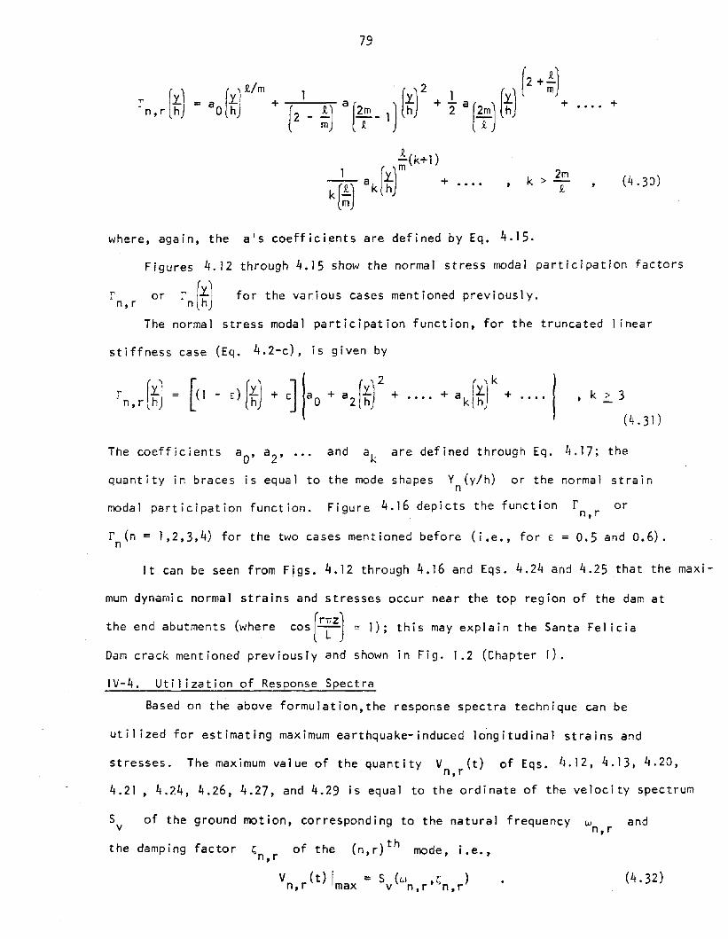
r (1.\n, r h)
= a [1.J 9.Jm +o h
79
• • •. +
k > 2m£,
(4.30)
where, again, the a's coefficients are defined by Eq. 4.15.
Figures 4.12 through 4.15 show the normal stress modal participation factors
for the various cases mentioned previously.
The normal stress modal participation function, for the truncated linear
stiffness case (Eq. 4.2-c), is given by
, k ~ 3
(4.31 )
The coefficients aD, a2
, ... and ak
are defined through Eq. 4.17; the
quantity in braces is equal to the mode shapes Y (y/h) or the normal strainn
modal participation function. Figure 4.16 depicts the function r orn,r
r (n = 1,2,3,4) for the two cases mentioned before (i.e., for E = 0.5 and 0.6).n
It can be seen from Figs. 4.12 through 4.16 and Eqs. 4.24 and 4.25 that the maxi-
mum dynamic normal strains and stresses occur near the top region of the dam at
the end abutments (where [rr.z) '" 1); this may explain the Santa Feliciacos --L
Dam crack mentioned previously and shown in Fig. 1.2 (Chapter r) •
IV-4. Utilization of Response Spectra
Based on the above formulation,the response spectra technique can be
util ized for estimating maximum earthquake-induced longitudinal strains and
stresses. The maximum value of the quantity V (t) of Eqs. 11.12,4.13,4.20,n,r
4.21, 4.?4, 4.26, 4.27, and 4.29 is equal to the ordinate of the velocity spectrum
the damping factor I;;n r of the (n,r) th mode, i.e.,,V (t) I = S (w I;; )n,r max v n,r' n,r
Sv of the ground motion, corresponding to the natural frequency wn,r and
(4.32 )

In",
)'~
0-1
l~I'
Gol'
/hl
h;;-1
NO
RMA
LST
RE
SSM
OO
Al
PAR
TIC
INTI
ON
FAC
TOR
r.h
/h)
-0.2
0-0
.10
00.
100
.20
i,
ilK
::::iii
I
0.9
0.80.1
~0
.2 In'
,I
~ 50
.3 iA.
B
1~I'GOI'/hl
~~
NO
RM
AL
ST
RE
SS
MO
DA
LP
AR
TIC
IPA
TIO
NFA
CTO
Rrn
(y/h
)
-0.2
0·0
.10
00.
100
.20
--r
,,
iKIii
i
In0.1
0.9
0.2
0.8
~ t-O.~
~ u ~0
4
ill r:0
.5~ o '" ~
0.6
-' z 9 ~0.
7:> i5
IP,-0
I
~ST
II£S
SM
OO
Al
IMT
IClN
TIO
NFA
CTO
Ilr.
I,/h
)
o-0
.20
-0.1
00
0.10
0.2
0iii
ilK
iii
I
C·.;
~
f).9
t; ~0.
3
~ ~0.
4:< ~ o
0.5
~ ... -' z ~O
.G
w :> 60
.7O.l!
-l~}
'GOI
"hl
i02~
hJ
MJR
MA
LST
RE
SSM
OD
AL
PAR
TIC
IPA
TIO
NFA
CTO
Rrn
{Y/h
l
-0.2
0-0
.10
00.
100
.20
Ii
II
Kiii
1.0
'J
,
(X)
o
[ft:4O
]
n:l
'I'"G
Il0
'_h
~):GO(Y/h)
h-,~
0-3
Go
NO
RM
AL
ST
RE
SS
MO
DA
LP
AhT
ICIP
AT
10N
FA
CT
0Rrn
(y/h
)
-0.2
0-0
.10
00.
10O
.t'O
iii'
,;;;;;:
IT
-"""'-
"",--
0.9
0.80.1
~0.
2
~0.
3
~0._
:z: Ii: ... o0
.5
III g0.6
iQ ~ 50.
7
IP,-20]
n"~
NO
RM
AL
ST
RE
SS
MO
DA
LP
tlRT
ICIP
AT
ION
FAC
TOR
rn(y
/h)
'0.2
0-0
.10
00.
100
.20
Iii
iKiii
O.l!
-hI~l
'Gol
"hl
°t~l~I-Go(Y/hl
~0
.2LG
~~.-
1
~0.
2h;;
-1t;
t;...
50
.35
0.3
'"So
..0 iil ..
a.
:<:z:
l-Ii:
.. ......
0o
0.5
0.5
~III
L6
~0
.6in
.!:l
z <oJ
...:>
,.U
0.7
~5
0.7
0.8
0.8
0.9
0.'
1.0
1.0
Fig
.4
.12
Nor
mal
str
ess
mod
alp
art
icip
ati
on
facto
rsfo
rth
ein
ear
case
.

NO
RM
AL
ST
RE
SS
MO
OAI
..P
MT
ICF
lIIT
ION
FAC
TOlIr.
(y/h
)N
OR
MA
LS
TR
ES
SM
OD
AL
PA
RT
ICIA
:\TIO
NF
AC
TO
Rr n
(ylh
)N
OR
MA
LS
TR
ES
SM
CID
AL
PA
RT
ICIA
l.TIO
NF
AC
TO
Rr n
(y/h
l
'0L
)I(
:
0.5
0-,
.·1
-0.2
5-0
50
0.1
0.2 1.
0-'
'''"-
--'1
0.8
0.9
, ~0
.3
"'u ~0
.4
l:l t05
\'J g: w0
.6
~\I
P,
.roJw
0.7
:> 6
0.8-0
.50
-0.2
50
0.2
50
.50
1i
lac:::
::::::
::::
it
02
0.90.1
!)I
fI
1.0
£ , f--
0.3
~ "'u 90.4
l:l ~0.
5
a '" g0.
6
ijl-
'i?
lB~
0.7
6
~!lO
-O.~
0.1·00!
lO
02
0.8 0.9
£ }. t;
0.3
l:! u ~O
·
~ ~0
5
\'J '" ~0
.6
~I~
¥!0
.7L.
.:.-..:J
"
I'"
I1.
0
co
.-,
r«»R
MA
LS
TR
ES
SM
()[)
aL
PA
RTI
CIP
ATI
ON
rl\C
TQ
Rr n
fylt
l)
__
__
O-~.()
-o.!I
O-l
IZ>
I..,I
~0.
1
0.2
¥. ~0
.3
0 ~0
.4
l!l ~0
5a '" ~
0.6
-' ~0
.,1E~
:> 0
0.8 09 If'
.'1
o.~
'0OoP0.2
0.1
£ }.
;:0
3
~ u ~0
.4
d ID ~0
5
a '" ~0.
61(
R,
-2°1
o ~0.
7~ 6
_M
AL
ST
RE
SS
MO
DA
LF
WlT
ICF
lIIT
ION
FM
:TO
Rr.
(yIh
)
·0.5
0-O.~
0o.~
().!
lOiil",,"=
=i
.'1
<'.I
}.
0.9
NO
RM
AL
ST
RE
SS
MO
DAL
..P
AR
TK
;IPA
TIO
NF
AC
TO
Rr n
(ylh
)
05
0-0
.25
00
.25
O.!l
OI
I-=
-i
I
0.8
(';
'
E(1
.-"
~l) ?:
(l·1
n ~ r.0" .. "' " ~06~!!f"~1
(; ~0,
7
~
Fig
.11
.13
Nor
mal
str
ess
mod
alp
art
icip
ati
on
facto
rsfo
rth
esq
uare
-ro
ot
case
.

1",/
>r
I
NO
RM
AL
ST
RE
SS
MO
ON
.P
MT
ICIl'
AT
IOH
FAC
TOR
r.
(,!h
I
.0
6.
0.3
00
.30
5Iii
__
II
0.1
~0
.2r
G"G
oIY
/h)1
I5
In 150,
3
m0
.41
n·3
% I- .. :O~~
Ifl,"
O!
~0
.6z '" " 5
0.7
0.8 o.q 1.0
NO
RM
AL
ST
RE
SS
MO
OIlL
PM
TIC
Il'A
TIO
NFA
CTO
Rr n
(y!h
)
.~
-~
0~
Mr
Ii
I1
0.1
~o.2
rG
"'G
oIY
/h)"
'
~0
.3 I04
% I- ..6
g:O.5~
~ ~0
.6
'"z '" " o0
.1
0.8 o.q
1.0
G"'G
oI.,/
tllI/
J
'~-i'::-"
'-O
JI-
..",
.""
LJl
'''.
'~
0.'::
'
0.8
NO
RM
AL
ST
RE
SS
MO
DA
LP
MT
ICIA
l\TIO
tlFA
CTO
Rr n
(y/h
l
•0.
.6•
0.3
00
.30
.6iiI
__
,I
~0.
3
S04
% I- .. ;o.~
rIfl,
'OI
~0
6
'"z ~ ;:50
.7
!0
.2
NO
RM
AL
ST
RE
SS
MO
ON
.P
MT
ICIl'
AT
lON
FAC
TOR
r n(y
/hl
.M
·0.3
00
3O
Ai
If
~02~'
GrG
o(y
/h)1
I1
I- '" 15
0.3
;0 ~0
.4% I-
~I;]
~O.5
~~ i06 , i3
0.7
0.8
!
o.q 1.0
NO
RM
AL
ST
RE
SS
MO
ON
.P
MT
lCIl'
AT
lON
FAC
TOR
rnh
llll
.0.6
.0.3
a0
.30
.5Iii
..II
OJ
!0
.2
~0.
3,
m0
.4% l- f! ;
o.t
1/1,02
01
i0.6 ~ a0
.1
0.8 o.q
1.0
NO
RM
AL
ST
RE
SS
MCl
Dr"I.
.P
lUrT
ICF
AT
ION
rlJl:.
TQ
Rr n
tylh
)
-Q
6_
Q3
00-
3o.£
,I
II
_1
----
OJ
~0
.2r
G°G
o(yJ
")'"
~0
.3
S0.4
% I- ~0.5
~Ifl
,.~1
gj ~0
.6
'"z ~ 00
.7 0.8 o.q
1.0
c:e N
Fig
.4.
14N
orm
alstr
ess
mod
alp
art
icip
ati
on
facto
rsfo
rth
eo
ne-t
hir
dcase
.

I.O~--------,)!I""---------,I
OJ
OO
RP.4
ALS
TRE
SS
MO
Olll
.PA
RTI
CIP
ATI
ON
fAC
TOR
rn(V
lh)
_0.6
_0
.30
0.3
0.6
rI
ii
I
G'G
,,lr"
"'"
~ .?:Q
3
In '" l50
4r!""
'01
3i '3 '".. :J:
0.5
I- .. ~ ::l0
.6
'"-' z 0 ~0
.7
"50
.8 0.9
I1.
0
G'G
,,(Y
"'J'"
0.3 ~T
B0
.5
0.6
0.7
0.8 0.9
I
1.0
NO
RM
AL
STR
ES
SM
ODAL
..PA
RTI
CIP
ATI
ON
fAC
TOR
f n(V
lh)
_0
.6_
0.3
00
.30
.6i
i~
i
~ ~ In ~ ~ '".. ~ '"a ~ -' § ~ '" "5
B
0.9
NO
RM
AL
STR
£SS
MO
DA
lP
AR
TIC
lMTI
ON
FAC
TOR
r n(,
,,,,
-0.6
•0
.30
03
0.6
----T
I==
===
i---,
G'G
"I,"
'J'"
OJI-~.j
.'"~
I,..
;iT,'.
:':';.
.,~h
0.21
-.,
'~
0.8
~0
.6
~ ~0
.7'" "5In
03
~ ~0
.4
ill ~0
.5
~i
00
Vl
G'G,,(~
NO
RM
AL
STR
ES
SM
()I)
jlL
PM
TIC
MlT
KlN
FAC
TOR
rnI,
ll»
M-~
0~
~i
I_
r----
NO~MAl
STR
£SS
MO
llAl
PAR
TIC
IPAT
ION
FAC
TOR
r.I,,,
,,M
-M
0M
M,
Iaaz
c:::::::
i
NO
RM
AL
STR
ES
SM
OD
Al.
PAR
TIC
RT
tON
fAC
TOR
r n(y
lh)
.0
.6_
0.3
00
.30
.6---1
lac:
::::
:==:
:I
I
G'G
"I""
""
OJ~~hI
,""/'~~~
"',:\.
..-=
0.2
'/h
,J/
ih
I~
I1
/I
/.'
2J
"=1
'Go
"~In
03
..,In
03
t;0
3..,
~~
[5~
04
~0
4t;
not
'"~
~-I~
ill1""
201
~L
III,'40
]ill
~0
5~
0.5
l'l0
.5..
a~
l:ll:l
:a0
6g
06
~Q
6g
'2~
..~
0.7
~0
.7~
0.7
5:>
55
0.8
0.8
0.8
0.'
0.'
0.9
1.0
1.0
1.0
Fig
.4.
15N
orm
alstr
ess
mod
alp
art
icip
ati
on
facto
rsfo
rth
etw
o-f
ifth
scase
.

:":"
:" I"~'
0.51
~~.)"",..)
hI~ Go
1-,'10
1
.·z
co
·'3
.'4
NO
RM
AL
ST
RE
SS
MO
OA
LP
MT
ICIP
AT
ION
FAC
TOR
rnl,
/h)
II
aa
'"N
OJ
,I
I
OJ
1.0
0.9'
0.11
iaz
t;; ~0.3
1
~0.4
X I- ~0
.5 i0.6 , 50
. 7
:":" --~
~
:"
~~.)"",..)
Gt
hI~
10---
<04
Go
.·4~'/
~/
~/
"'-2I.
.·,
NO
RM
AL
ST
RE
SS
MO
OA
LF
'MT
lC,P
AT
ION
FA~TOR
rnl,
/h'
II
coco N
o
0.9 I.O
L_
_~~_V.
_
0.11OJ
ioz
t;; ~0.
3
~ it0.
4X e o
0.5
III ~0
.6
i 00
.7
~
.'1
("~'
0.51
~~.)"",..)
Gt
hI~
10---
<04
Go
n'3
".4__~""--
NO
RM
AL
ST
RE
SS
MO
OoI
LF
'MT
'CIP
ArI
ON
FA
CT
OR
rnl,
/h}
JJ
0.
.N
Q~
&m
0'"
0.11 I~l
V~
OJ
0.9'
iO
.z
t;; ~a3
i
~0.4
X l- e o0.
5III i0
.6~ ~ 0
0.7
(Xl
.l::-
~
G..J
'"'"",,
,)
hI~ .... Go
<>
·'3
.·4
NO
RM
Al.
ST
RE
SS
MO
DA
LP
AR
TIC
IPA
TIO
NrA
CT
OR
r"(y
/h1
dd .r
._..
.
01i
II
I
0.8 0.9 1.0
OJ
io.
Z
t;; ~0.
3:
! iii0
4X to: ... o
0.5
III ~0
6~ , 0
0.7
co
B
I..~
.0
61
~ .·z
G..JI
.•}y
Ih••j
hI~ .... Go
.~
.'3
:"
·'4
NO
RM
AL
ST
RE
SS
MO
OA
LF
'MT
lC,P
AT
lON
FAC
TOR
rnl,
/h)
~a'
0.11OJ~
~u
.v_
_.
Oi
iI
I
0.9 1.0
~oz
In ~0.
3
~ iii0.
4X to: :!:
0.5l!! ~
06
j o0
.1
.·z G..JI
.•,yIh
••)
Go
hI~ .... Go
.'3
.·4
0.11 0.9
OJ 1.0"
ioz
t;; ~0.
3'
! iii0.
4X l- e o
0.5
III ~0
.6
~ 50
. 7
NO
RM
AL
ST
RE
SS
MO
DA
LfM
TIC
IPA
TIO
NrA
CT
OR
rn(y
/h)
,,
~?
aa
~~
'"
Fig
.4
.16
Nor
mal
(wi
thstr
ess
mod
alp
art
icip
ati
on
facto
rsfo
rth
etr
un
cate
dcase
£=
0.5
and
0.6
).
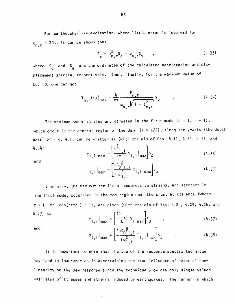
85
For earthquake-l ike excitations where 1ittle error is involved for
r; n, r < 20%, i t ca n be shown t ha t
Sa
2= w S = w Sn,r d n,r v
(4.33)
where Sandd
S are the ordinates of the calculated acceleration and disa
placement spectra, respectively. Then, finally, for the maximum value of
Eq. 10, one can get
~= _4 __n~,=r==::;::::. S
rn w v'1.- r;2 1 vn,r n,r
(4.34)
The maximum shear strains and stresses in the first mode (n = I, r = I),
which occur in the central region of the dam (z ~ L/2) , along the y-axis (the depth
axis) of Fig. 4.1, can be written as (with the aid of Eqs. 4.11,4.20,4.21, and.'.
4.34)[4P J
'Y I 1 'max_ I, I 1j! S (4.35)- nh 1,1 Imax d,
and .'.
[4Gil I °1)max}a (4.36)T I = 'I, I max h 2
n WI 1,
Simi larly, the maximum tensile or compressive strains, and stresses in
the first mode, occurring in the top region near the crest at its ends (where
z ~ L or cos(rnz/L) ~ I), are given (with the aid of Eqs. 4.24, 4.25, 4.26, and
4.27) by.'.
maxh[4P 1,1
E .\ = L VI1,1 max
and[4nGo: I•I rl.llmax]sa0'1 , I Imax =
LW I 1,(4.38)
It is important to note that the use of the response spectra technique
may lead to inaccuracies in ascertaining the true influence of material non-
linearity on the dam response since the technique provides only single-valued
estimates of stresses and strains induced by earthquakes. The manner in which

86
the amplitudes of an earth dam's motion vary with time have a major role in
the dam's earthquake response characteristics. In the next chapter a rational
method is presented which takes into account this variation, also using the
elastic analytical models.


87
CHAPTER V
IDENTIFICATION OF CONSTITUTIVE RELATIONS, ELASTIC MODULI,AND DAMPING FACTORS OF EARTH DAMS FROM THEIR EARTHQUAKE RECORDS
V-I. Basis of the Analysis
The dynamic soil properties which exert the greatest influence on an
earth dam's dynamic responses are those related to the stress-strain relations.
Like all soils, materials of earth dams develop nonlinear inelastic stress-
strain relationships when subjected to earthquake loading conditions. By
using earthquake response records of the crest and the base (structural and
input ground motions), together with the results of the analytical models
(presented here), these stress-strain relationships can be estimated for the
dam's materials. The strain-dependent elastic moduli and damping factors have
already been determined in this manner for the upstream-downstream recorded
motion of a modern earth dam (see Refs. 1, 4, and 6), using existing analytical
shear-beam models (9, 22, 23).
One of the purposes of this report is to present a similar procedure (like
the one developed by Abdel-Ghaffar and Scott, Ref. 6) to estimate longitudinal
dynamic stresses and strains and corresponding elastic moduli and damping fac-
tors for earth dams from their hysteretic responses to real earthquakes, util-
izing the hysteresis loops from crest and base records and the above-mentioned
longitudinal elastic analytical models.
The idea is illustrated in Fig. 5.1 and can be summarized in the following
steps:
(1) By using the earthquake records, the experimental results and the
analytical models (of Chapters I I and IV), the fundamental frequency in
longitudinal direction can be identified.

88
- ..
NONLINEARRESTORING. XFORCE ...--...._-F(l,i)
r-->
l,W
- ...
CrestAccelerograph
,..
[.~ ......~ t
h -: Nonlinear Materia I ::. ~~'l-r..:r':.....~t.'":"':':'•• ,::-::.,:ol.:-::::.,:i:..."",";-r.;:.-;::-:::••"::,......s~,~.1::'.!"':'.'O'.::r.~
ty,v Wq(t)
-----.~wq(t)
y,v
MODEL REPRESENTING REAL EARTH DAM EQUIVALENT SYSTEMHYSTERETIC SINGLE- DEGREE-OF- FREEDO'" O~GILL
Stress
Strain
)"1 )"2
I'TYPical HystereticShear Stress - StrainRelationships (Soil)
W(t)
EarthquakeHystereticResponse
x
.J' ke1
HystereticResponse
,/
EQUIVALENT SYSTEM EARTHQUAKE RECORDS EARTHQUAKE RECORDS ANDANALYTICAL MOOELS
Fi g. 5.1 IDENTIFICATION OF ELASTIC MODULI AND DAMPING FACTORS FROM
EARTHQUAKE RECORDS

89
(2) By using very narrow band-pass digital filtering around the funda-
mental frequency (usually the primary) of the crest and base records,
the pure fundamental mode response can be obtained.
(3) By treating the filtered modal response as that of a single-degree-
of-freedom (SDOF) hysteretic structure (with nonlinear restoring
force F(x,x) equal to -M(x + w(t)); x,g x, and x are the
relative displacement, velocity, and acceleration, respectively,
and M is the mass) the hysteresis loops, which show the relation-
ship between the relative displacement of the crest with respect to
the base and the absolute acceleration of the dam, can be obtained.
(4) By using the elastic longitudinal analytical models, the shear
stresses and shear strains (Eqs. 4.35, 4.36) can be determined as
functions of the maximum absolute acceleration and maximum relative
displacement, respectively, for each hysteresis loop, and consequently,
equivalent (secant) shear moduli and damping factors can be deter-
mined from the slope and the area, respectively, of the loop. Since
it was assumed that each hysteresis loop is a response of an SDOF
oscillator, and in order to get a qualitative picture of the dynamic
shear strain and stress from the hysteretic response, the value of
Sd and of Sa in Eqs. 4.37 and 4.38 are assumed to be the maximum
relative
eration,
Finally,
displacement, (w(t)) ,and the maximum absolute accel-max
(w(t) + w (t)) ,respectively, for each hysteresis loop.g max
the data so obtained permit development of typical stress-
strain curves which are then approximated by the Ramberg-Osgood
analytical models and/or the hyperbolic curves. The data can also
be compared with those previously available from soil-dynamic
laboratory investigations and can be combined with those obtained
90
from the analysis of the upstream-downstream vibrations (Ref. 6)
to give informative materials to both earthquake and the geotechnical
engineers.
V-2. Application of the Analysis
V-2.1. Longitudinal Dynamic Shear Stress-Strain Relations for Santa Fel iciaEa rth Dam
The Santa Felicia Dam (I, 3, 4, ~ is equipped with two accelerographs
(one on the central region of the crest and the other at the base) that
yielded data on how it responded to two earthquakes (1,4).
Amplification spectra of the dam's two earthquake records which were
(presented in Chapter I I I) computed by dividing Fourier amplitudes of
acceleration of the crest records by those of the base records (to indicate
the resonant frequencies and to estimate the relative contribution of differ-
ent modes in the longitudinal direction) revealed that the values of the
resonant frequencies vary slightly from one earthquake to the other. In
addition, amplification spectra of the upstream-downstream direction showed
that the dam responded primarily in its fundamental mode in that direction,
but the spectra of the longitudinal component are lacking pronounced single
peaks.
For Santa Fe1 icia Dam, the first longitudinal frequency determined from
the amplification spectra of the 1971 earthquake is 1.35 Hz (1.27 Hz for
2 4the 1976 earthquake), p = 4.02 1b-sec 1ft, v = 0.45 (3), and hlL =
2236.5/912.5 = 0.26; this gives 8r = 1.92 r , r = 1,2,3, .... (or 81 = 1.92 for
the first mode). The calculated shear stress and shear strain modal partici-
pation factors, along the depth of the dam, ¢n,r (or ¢ n = 1 and 2)
n'and
'¥n,r (or '¥ , n =1,2, and 3), as well as the normal stress modal particin
pat ion factor rn,r (or r,n=l)n
for various stiffness variations are

91
shown in Figs. 5.2a, b, c, and d. The first-mode maximum shear strains for the
analytical models of various stiffness variations occur at about 0.4 - 0.7
of the dam height (except for the linear case, where £/m = 1, in which the
maximum occurs at the crest). The maximum shear stress occurs at about 0.7 -i'{
0.8 of the dam height. Values of the participation factors PI l' ~ I, I max'
~ I r I resulting from the modal configuration along the depth and1 max' I max
the corresponding maximum strains and stresses (Eqs. 4.35,4.36,4.37, and 4.38) are
given in Table 5.1; also shown in the tables are values of vsO (and GO)
estimated from the 1971 earthquake records and the various analytical models
of Chapters I I and IV.
In general, it was found that the higher modes make a considerable con-
tribution to the overall earthquake response ·of the dam (displacements,
stresses, etc.); this is consistent with the earthquake amplification spectra
of Fig. 3.3-c.
The average maximum shear strain (percent) for each hysteresis loop, of
the 1971 earthquake. (Eq. 4.35) can be given by
Yl 11 = 0.04078 w(t) I, max max(w in cm)max
and the associated average maximum shear stress (in psf) of Eq. 4.36 is given by
= 11.78 (w(t) + w (t)) .g max2
(accelerations are in cm/sec )
(5.2)
The maximum (average) values of axial stresses and strains (from Eqs.
4.37 and 4.38) are:
E 1,1 Imax = 0.02773 w(t) I , (wmax in cm)max
and
0 1,1 1 max = 14.35 (w(t) + wg(t))max
(accelerations are2
in cm/sec ).
(5.4)
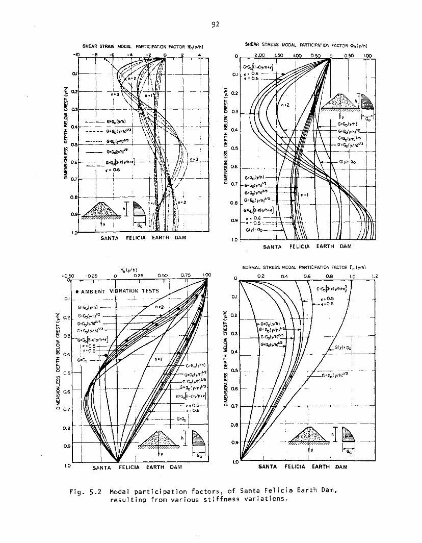
92
SANTA FELICIA EARTH DAM
SI:fEAR STRAIN MODAL PARTICIPATION FACTOR "'n(y/h)
-10 -2 0 2 4
G'Go(y/h) --+I-~I-#J----.""""'~N
G.GrJ.ylh)If2_--'lf----;~
G.Gt,(ylh)Zf5 -+--4HI~\
G=Go(y/h).,3 -itr---tto-lll-1Ht~--t--+-\+---+~""+-l
G'Gt>~I'C)yIh+£]
c= 0.6£ • 0.5 --=-.:~, ,c- -=-n'TTI
0.7
0.8
0.5
0.9
~loJ
~Vi 0.6zUJ::;:C
0.1
2~ 0.2
Il!liiu 0.3
SHEAR STRESS MODAL PA'mCIPATION FACTOR C:>n (y/h)
y
,tG-GrJ.'f/h)Vl i
_,_,_,_ G'Gt>~I.C)ylh+C]c·0.6
I
",'In =2
;a ~-+IiI ..~..~:~-,----
.h:1 :r(:~ i)j .1•.~__..... U"'O"Iill..J1I-...w.I.-I.-__..J
0.6
OJ~--t-
~ 0.2~--t--
~U 0.3
~
~ 0'4t------~-r4'.,f:x
~o 0'5t-----=G:.....=(y:....~=--_i_-____1~\.:._+_
SANTA FELICIA EARTH DAM
0.7
0.5
0.4
~loJ
~Vi 0.6zloJ::IiC
0.1
0.9
SANTA FE UClA EARTH DAM
1.0 L-__~_-""__....l..__~__~_---J
NORMAL STRESS MODAL PARTICIPATION FACTOR r n (y/h)
o 0.2 0,4 0.6 0.8 1.0 1.2
~
~IS 0.3:it 1----4
~a:>:x~loJo
0.8
2~ 0.2
1.00
/4---~<,w-r- G=Go(y/h)
H>W-+--- G=Go(y/h),f2
/ ~fH--T--G'Go{Y/h)V5
-j;flr#~*,-,='-G =Go( y/h)"3
G=Go[(I' c) y/h HJ- C =0.5-
/b<.L---+--- £ = 0.6
SANTA FELICIA EARTH DAM1.0
0.9
0.5
0.7
Yn (y/h I-0.50 0.25 0.50
Or-...,....-.:..-r----T---.....-...,....-M--Tr""-~
~UJoJ
6Vi 0.6zUJ::;:C
0.1
• AMBIENT VIBRATION
0.8
G=GO(y/h)
G=Gofy/h)'12 --f---:::;-;L:----:::l~~~
~ G'Go(Y/h)V5 __I--_t!.----::~~Q'
~ G=Go(y/h)lf3_-+~:""""--:~~V
U 0.3 r. ]'G=Gt,lO·£) ylh+£
~ I £= 0.5+--I--1~~ra:> 0.4 : £=0.6:x~a.UJo
2~ 0.2
Fig. 5.2 Modal participation factors, of Santa Felicia Earth Dam,resulting from various stiffness variations.
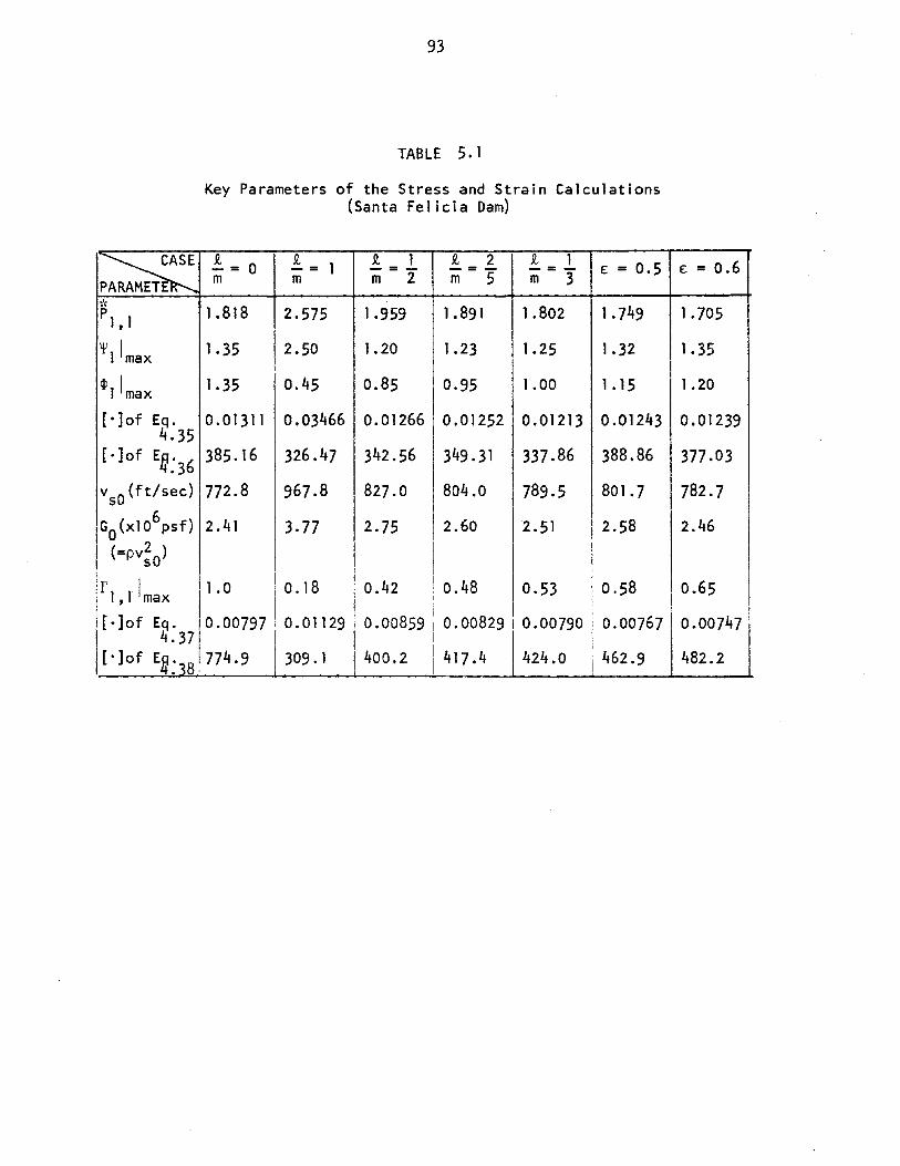
93
TABLE 5.1
Key Parameters of the Stress and Strain Calculations(Santa Felicia Dam)
~R, R,
1R, I R, 2 R, I
£ = 0.5 e: = 0.6-=0 - = - =- -= - -= -PARAMETE m m m 2 m 5 m 3
* I .818 I .891 1.802 1.749PI, I 2.575 1.959 1.705
'!'Il max 1.35 2.50 1.20 1.23 1.25 1.32 1.35
epl1max 1.35 0.45 0.85 0.95 1.00 1. 15 1.20
[. ]of Eq. 0.01311 0.03466 0.01266 0.01252 0.01213 0.01243 0.012394.35
[·]of Et36 385.16 326.47 342.56 349.31 337.86 388.86 377 .03
vsO(ft/sec) 772.8 967.8 827.0 804.0 789.5 801.7 782.76 2.41 2.60 2.58 2.46GO (xl 0 pst) 3.77 2.75 2.51
(=pv2 )sO
rl,llmax 11.0 0.18 0.42 0.48 0.53 ! 0.58 ! 0.65I!
[ . ]of Eq. 0.00797 0.01129! 0.00859 0.00829 I 0.00790 i 0.00767 i 0.007474.37 I
[·]of Et~8 774.9 309.1 I 400.2 417.4 424.0 462.9 482.2

94
In the above equations, w(t) is the maximum relative displacement inmax
each hysteresis loop, and (w(t) + w (t)) is the maximum absolute accel-g max
eration in each hysteresis loop. Figure 5.3 shows the filtered records (1971
earthquake) of both the absolute acceleration (crest record) and the relative
displacement (the crest response with respect to the base). It is important
to note that the first 3.0 - 3.5 secs of the base record were lost due to
double exposure (1,4). The time dependence of the hysteretic behavior was
determined for only the first 25 secs of the 1971 record and for only the
first 6 secs of the 1976 record. Each trajectory was plotted every 0.02 sec,
and each loop was plotted every second (about every cycle and a half).
Samples of the hysteresis loops (of the first mode of longitudinal vibration)
of Santa Fel icia Dam are shown in Fig .. 5.4. (Appendix A shows unfiltered records.)
It is readily apparent that the slope of the hysteresis loop and the
area inside the loop are dependent on the magnitude of the response level for
which the hysteresis loop is determined.
The estimated shear strain and stress for each hysteresis loop are shown
(as circles) in Fig. 5.5; the data show an initial slope, Gmax ' at the origin
ranging from 3.5 to 4.10 (x 106 psf). The nonlinear stress-strain curves
of the Masing type, i.e., the Ramberg-Osgood (R-O) curves (31,32) are
adopted here to fit the data (shown as solid curves on Fig. 5.5). For shear-
ing stresses increasing from zero these strain-softening curves are described
by
where a and R are parameters which adjust the position and shape of the
is a factor which relates the I'yield" value
For practical and
curves, and
original R-O expression to Tmax(i.e., T = CIT ).y max
TY
in the

95
SAN FERNANDO EARTHQUAKE FEB 9 1971SANTA FELICIA DAM. CALIFORNIA. CRESTLONG I TUD I NAL COMPONENT (S75W)
..'\I V \I
&
-8OO~_-!.-L----4------+---+----+----+-----+----+----+---_---40.00 5.00 10.00 15.00 20.00 25.00 30.00 35.00 '0.00 ~.OO 50.00 55.00
TIME IN SEC
22.0
>- 1'.0~
......-ufj •. OOlf)-l'W~-2.0>~
20.00 25.00 lID. 00 ".00 ~.OO ~.OO SO. DO 55.00
TIME IN SEC
-10'~__+-__+---__~_--+__-+__--+-__--+-__-+-__+-__+---_--4O.DO 5.00 10.DO 15.00
~
Z 1.20W2:W 0.10U0:_...J~ 0.00Q..~tn~ -o.to
-t.20I~__~---4__--+__--+-__-+-__-+-__-+-__+-::-----:-t-":':_~:-=_~
0.00 5.00 10.00 15. DO 20.00 25.00 lID. 00 15. DO '0.00 ~.OO so. DO 55. DO
TIME IN SEC
Fig. 5.3-a The filtered records (1971 earthquake) of the crest ofSanta Felicia Dam.

SAN FERNANDO EARTHQUAKE FEB 9 1971SRNTA FELICIR DAM, CALIFORNIA, OUTLET WORKLONG ITUD I NRL COMPONENT IS82Wl
.12001-.oo--.....5~.1IU---410-.oo---+15-.DO--l-+0-.DO--c:'t"5--::.0-=-0---::3+-0.-=0=-0 -~4t-'i.-=00=----:""ot-.:::00:---j"5;-.oo;::--;t50:-:.0::;:O-~55.00
TIME IN SEC
l.tI _
>- O.C _
-I.Z 1------<I---___l--__+----+----+--_---+---~--_+_--_+_-____10.00 5.00 10.00 1'i.00 ZU.OU Z5.00 30.UU 35.00 flO. 00 45.00 50.00 55.00
TIME IN SEC
~
Z U.lie.UJ~
UJ O.DC.Ucr.~
~~ 0.00CL. J
(J)
~ -0.
-o.IZI-:----::+-:---~~-_t_::__-:t_:::__-"'::_:---:::+:___:_:__-+__:_:__-~----l-:------+----40.1IU 5.00 10. lID lS.DO 20. DO ,!"i.ou 10.00 35.00 "O.DO ~5.lkJ SO. DO 55.DO
TIME IN SEC
Fig. 5.3-b The filtered records (1971 earthquake) of theabutment of Santa Felicia Dam.

97
5AN FERNAND~ EARTHQUAKE FEB 9 1971 SANTA FELICIA DAM, CALIF~ANIA
RELATIVE ACCEL., VEL. AND DISP. ~F CREST W.R.T. ABUTMENTC~MP~NENT R~TATED PARALLEL T~ DAM AXIS lS78.6W)
-1UUU\----+---+----+----+---+:---1---+----±'~-_+:__=_____:±_-__:!D.DO 5. DO ID.DO 15.DO 2D.00 25.00 SO. 00 !5.00 Illl.DO U.DO SO. DO 55. DO
TIME IN SEC
12.0
>- '.0~....-Utj 0.00(1')...J'~
~8-e·D
-12.D.DO 5. DO lD.DO 15.00 20. DO 25.00 SO. DO '5.00 'D. DO '5. DO SO. DO 55. DO
TIME IN SEC
~
z 1.2DWz:W 0.10Ua::_...J~ D.DO0..8(J').... -0.0
-I.D.DO 5.DO 10. DO 15.DO 2D.DO 25.00 SO. DO !5.DO Illl.DO U.DO SO. DO 55. DO
TIME IN SEC
Fjg. 5.3-c The fjltered records (1971 earthquake) of therelative motion (the crest response with respectto the base) of Santa Fe1 icia Dam.

EARTHQUAKE OF APRIL 8, 1976SANTA FELICIA DAM, CALIFORNIA, CRESTLONG I TUD I NAL COMPONENT 1578. 6W)
18.DO".DDI.DD•• DD2.DD~--+----+----..----t-------<t---~I---~-----+----+-~
18. DO 20. or-10
D.OO
'.D
>- •• Dt---U~D.DO<n-Ji:WX--O>.....,-...
.... D01-.DD---2......DD---.......DD---I~.DD---.~.DD------Il0~.-DD-----l12>-. DD--~"-.DD---+lIl-.00--1-+11-.O-O---:iZO •Ot
TIME IN SEC
t-Z D.IOW2:W D.'DUCI:_-J~ 0.000...en-o
O.DD 2.DD '.DD I.DD
Fig. 5.3-d The filtered records (1976 earthquake) of thecrest of Santa Felicia Dam.
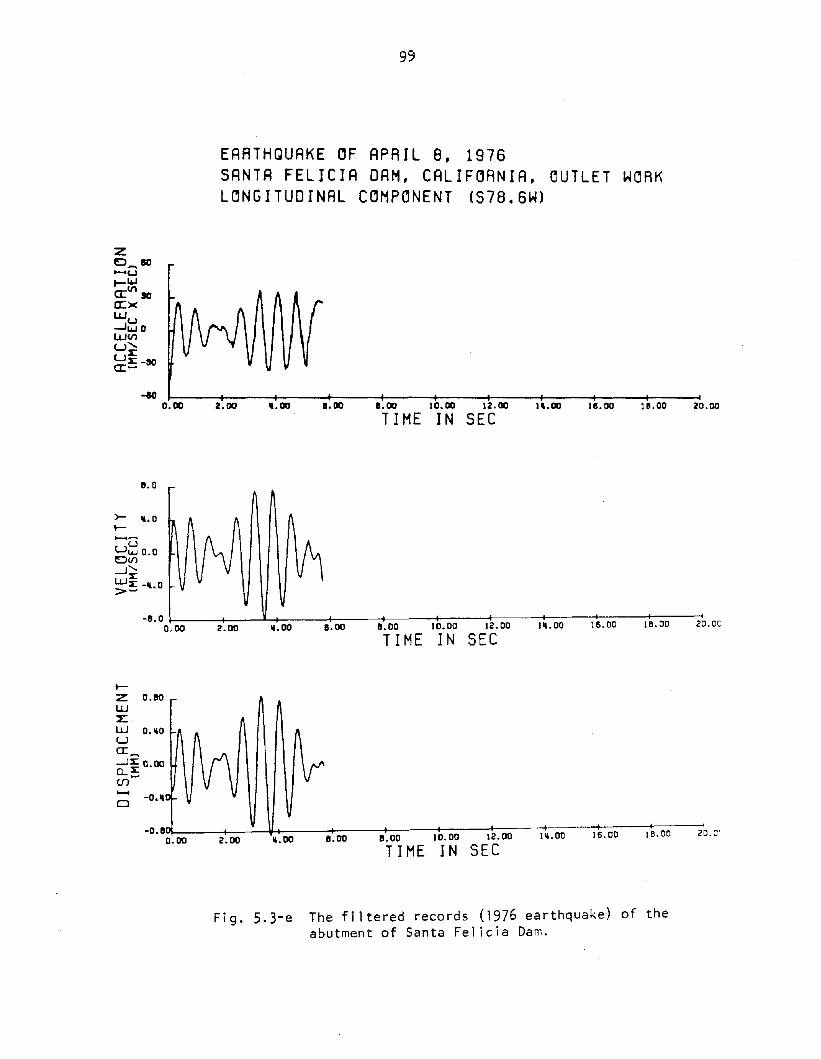
99
EARTHQUAKE OF APRIL 8.1976SANTA FELICIA DAM. CALIFORNIA. OUTLET ~ORK
LONG ITUD INAL COMPONENT (S78. 6~)
-eo0.00 2.00 ll.OO 8.00 11.00 10.00 12.00
TIME IN SEC18.00 111.00 20.00
11.0
>- ll.Ot---u~o.oDcn-J.......
x:~~-ll.O
-11.00.00 2.00 ll.OO 8.00 11.00 10.00 12.00 11l.00 16.00 18.00 20.0C
TIME IN SEC
t-z 0.110UJ~
UJ O.llOUCI_-J~ 0.00D....~(f)- -O.ll0
-0.1110.00 12.00 Ill.OO 16.00 18.00 20.0'
0.00 2.00 1l.00 8.00 11.00
TIME IN SEC
Fig. 5.3-e The filtered records (1976 earthquake) of theabutment of Santa Felicia Dam.

100
EARTHQUAKE OF APRIL 8, 1976, SANTA FELICIA DAM, CALIFORNIARELATIVE ACCEL., VEL. AND DISP. OF CREST W.R.T. ABUTMENT
LONG I TUD I NAL COMPONENT (578. 6W)FJLT£ftJNG TYPE t
-so0.00 2.00 S.DO 8. DO 10. DO 12.00
TIME IN SECn.oo 15.00 18.DO 20.00
8.0
~ '.0t---U~O.OOVl...J's::~~ -4.0
-B. 0O.DO 2.00 '.00 1.00 '.00 10.00 12.00 1'.00 11.00 18.00 20.00
TIME IN SEC
t-z 0.10UJ%:UJ 0.'0U0:_...J~ 0.000......,en-0
-0.100.00 2.00 '.00 '.00 '.00 10.00 12.00 I'.DO 18.00 11.00 20.00
TIME IN SEC
Fig. 5.3-f The filtered records (1976 earthquake) of therelative motion (the crest response with respectto the base) of Santa Felicia Dam.

101
SANTA FELICIA DAM, CALIFORNIA,COMPONENT ROTATED TO LONGITUDINAL DIRECTIONH,STERETIC RESPONSE FILTERING TIPE C
120 120
-80
-120
1 - 2 SEC
~ -00:J-loCf)
~ -12.0 L-_---lL.-_--l.__--1-.__--J
z 0£)........a:cclU-llUU
~
8 80enxulU 110~:s:
·u~
o - 1 SEC
B 80enxu~ 110"':s:8z 0D........a:a::lU-llUUUa:lU....:J-lD",coa:
-2.0 -1.0 0.0 1.0 2.0 -2.0 -1.0 0.0 1.0 2.
RELRTIVE OISPLRCEMENT (CM) RELRTIVE DISPLRCEMENT (CM)
12.0 120
3 - II SEC
tj 80Cf)
xu~ 110"'::E:U
z 0D....a:cc~ -110lUuua:
~ -80:J-loVl
~ -120 L-_---lL.----L----1-.--.....J
2 - 3 SEC
z 0£)........a:cc~ -IUJlUuua:
~ -80:::l
5Cf)
~ -120 L...-_.......JL.....-_---t.__~__....J
8 80enxu~ 110~u...
-2.0 -1.0 0.0 1.0 2.0 -2.0 -1.0 0.0 1.0 2.0
RELRTIVE OISPLRCEMENT (CM) RELRTIVE DISPLRCEMENT (CMI
Fig. 5.4-a The hysteresis loops (of the first mode of longitudinalvibration) of Santa Felicia Dam (1971 earthquake).

102
SANTA FELICIA DAH, CALIFORNIA,CCHPCNENT ROTATED TC LCNGITUDINAL DIRECTIONHYSTERETIC RESPONSE FILTERING TYPE C
120 120
U -60 u BO"-l "-len en)( )(
u U"-l "0 "-l tWen en.... ....:I: :I:8 8
l5 0 z 00- -~ ~cr cra:: a::
"-l -"0. "-l -"0..J ..J"-l WU UU Ucr cr"-l -80 w -BO~ ~
~ ~..J " - 5 SEC ..J 5 - 6 SEC0 0If) If)
lD-120 lD
-120cr a:
-2.0 -1.0 0.0 1.0 2.0 -2.0 -1. a 0.0 1.0 2.0
RELATIVE DISPLACEMENT (CJ1) RELATIVE DISPLACEMENT (eM)
120
U 80wen)(
uw ijOen....:I:U--5 0-~cra::w -"0..JWUUcrw -80~
~
..J[;)enlD -120cr
f-
I(f!J
6 - 7 SEC
120
u BOwen)(
uw "0en....:I:U--Z 00-~cra::w -"0..JWUUcrw -BO.--~..J0enlD -120a:
~
6
7 - 8 SEC
-2.0 -1.0 0.0 1.0 2.0 -2.0 -1.0 0.0 1.0 2.0
RELATIVE OISPLACEHf~T (CH)
Fig. 5.4-a (continued)
RELATIVE DISPLACEMENT (CH)

113
SANTA FELICIA DAM. CALIFORNIA.COMPONENT ROTATED TO LONGITUDINAL DIRECTIONHYSTERETIC RESPONSE FILTERING TYPE C
120
u 80w(f)
x
uw ~o(f)
"-:s::u-z 00
I-
exa::w
-~O...J...JUUexw -80I-
~...J0(f)CD -120ex
~
J
~
8 - 9 SEC
120
U eo...,(f)
)(
u
""' '0(f)
"-EU...Z 0C-....a:a::""' -qO...J
""'UUa:loJ -80....::l...JC(f)CD -120a:
~
~j)
9 -10 SEC
-2.0 -1.0 0.0 1.0 2.0 -2.0 -1.0 0.0 1.0 2.0
120
U 80w(f)
xuw ~O(f)
"-:s::~
z 00
I-a:a::w -ijO...JWUUexw -80I-~...J0(f)CD -120ex
RELRTIVE DISPLRCEMENT (CM)
1/I
10- 11 SEC
120
U 80""'(f)
xu""' '0(f)
"-EU...Z 0C-....exa::
""' -I!O..J
""'UUa:
""' -80....::l
E(f)CD -120a:
RELRTIV[ DISPLRCEMENT (CM)
rII
11- 12 SEC
-2..0 -1.0 0.0 1.0 2.0 -2.0 -1.0 0.0 1.0 2.0
RELRTIVE DISPLRCEMENT (CM)
Fig. 5.4-a (continued)
RELRTIVE DISPLRCEMENT (CM)

101:
SANTA FELICIA DAM, CALIFORNIA,COMPONENT ROTATED TO LONGITUDINAL DIRECTIONHYSTERETIC RESPONSE FILTERING TYPE C
120
U 80\oJVl
X
U\oJ ~OVl.....:I:~
z 00-~a:a::\oJ
-~o....J\oJUUa:\oJ -80~....J0VlCD -120~
V/
12-13 SEC
120
U 80IIJenxuIIJ lWVl.....:I:U..-
~0-....a:
tr:\oJ -lW....J\oJUUa:\oJ -80~6VlCD -120~
VI
13- 1li SEC
-2. 0 -1. 0 O. 0 1.0 2.0 -2.0 1. 0 0.0 1.0 2.0
120
U 80\oJVl
X
U\oJ ~OVl.....:I:
~
z 00
~
a:a::\oJ -1l0....J\oJUUa:\oJ -80~;:)....J0VlCD
-120a:
RELRTIVE DISPLRCEMENT (CM)
~
I
l~-lSSEC
120
U 80\oJVl
X
U\oJ ~OVl.....:I:U..-
Z 010-...a:a::l&J
-~O-'IIJUUa:\oJ -80...;:)....J10VlCD -120a:
RELRTIVt DISPLACEMENT (CM)
~
~
15- 16 SEC
-2.0 -1.0 0.0 1.0 2.0 -2.0 -1.0 0.0 1.0 2.0
RELRTIVE DISPLRCEMENT (CM)
Fig. 5.4-a (continued)
RELRTIVE DISPLRCEMENT (CM)

lOS
SANTA FELICIA DAM, CALIFORNIA,COMPONENT ROTATED TO LONGITUDINAL DIRECTIONHYSTERETIC RESPONSE FILTERING TYPE C
120
0 80IoJVI
)(
UIoJ qOVI"-~u....z 0IC-....crlZ:IoJ -qO-JIoJUUcrIoJ -80....:::l-JICVIID -120cr
It,
16-17 SEC
120
-u eo»:)(
u
"" "0en"-EU...Z 0IC-....cra::
"" -1£0-J
""UUa:
"" -80....:::l-JICenI:)
-120a:
~
III
~
17-18 SEC
-2.0 -1.0 0.0 1.0 2.0 -2.0 -1.0 0.0 1.0 2.0
120
0 80IoJVI
)(
UIoJ qOVI"-~
8z 0IC-....crlZ:IoJ -qO-JIoJUUcrIoJ -80....:::l-JICVIID -120cr
RELRTIVE DISPLRCEMENT (CM)
I~
~
18- 19 SEC
120
0 80IoJen)(
u
"" "0en"-EU...Z 0IC-....a:II:
"" -1l0-J
""UUcrIoJ -80....:::l-JICVIID -120a:
RELRTIVE DISPLRCEMENT (CM)
,~
~
19- 20 SEC
RELRTIVE DISPLRCEMENT lCM)
-2.0 -1.0 0.0 1 0 2.0 -2.0 -1.0 0.0 1.0 2.0
RELRTIVE DISPLRCEMENT (CM)
Fig. 5.4-a (continued)

lOG
SANTA FELICIA DAM, CALIF~RNIA,
C~MP~NENT R~TATED T~ L~NGITUDINAL DIRECTI~N
HYSTERETIC RESP~NSE FILTERING TYPE C
RELRTIVE DISPLRCEMENT (CM)
ItI
20- 21 SEC
120
u 80w(f)
xuw ~Oen"-x:8z 00
~
a:a::w -1l0...JwUua:w -80~
:;)...J0(f)Q:)
-120a:
-2.0 -1.0 0.0 1.0 2.0
120
U BOwen)(
uw 110en"EU...Z 00-....a:cz:w -1l0...JwUua:w -80....;:)...J 21-22 SECc(f)Q:)
-120a:
-2.0 -1. 0 0.0 1.0 2.0
RELRTIVE DISPLRCEMENT (CM)
120
U 80w(f)
xuw 110en"-x:8z 00-....a:a::w -1l0...JwUua:w -80~:;)...J0enQ:)
-120a:
Ifj
22- 23 SEC
120
U 80w(f)
)(
uw 110en"-x:8
~0-....a:cz:
w -1l0...JwUua:w -80....;:)...JCenQ:)
-120a:
1
23- 2" SEC
-2.0 -1.0 0.0 1.0 2.0 -2.0 -1.0 0.0 1.0 2.0
RELRTIVE DISPLRCEMENT (CM)
Fig. 5.4-a (continued)
RELRTIVE DISPLRCEMENT (CM)

107
SANTA FELICIA DAM, CALIFORNIA,COMPONENT ROTATED TO LONGITUDINAL DIRECTIONHYSTERETIC RESPONSE FILTERING TYPE C
60 60
1 - 2 SEC
-20
z ac-~a:a::l&J-ll&JUUa:
E 110(f)
)(
u~ 20"s:s:...
o - 1 SEC
-~ 110(f)
x
u~ 20"xx'-'
~
a:a::~ -20wuua:
~ -1l0~-lC(f)
~ -60
z 0c
-1.0 -0.5 0.0 0.5 1.0 -1.0 -0.5 0.0 0.5 1.0
60RELRTIVE DISPLRCEMENT (MM)
60RELRTIVE DISPLRCEMENT (MM)
-~ 110(f)
x
u~ 20"xx
z 0c~
a:a::~ -20wuua:
~ -1l0~-lC(f)
~ -60
2 - 3 SEC
E 110CIl
)(
U~ 20"s:s:...z 0c~a:a:~ -20l&Juua:~ -1l0~-lCCIl
~ -60
3 - Il SEC
RELRTIVE DISPLRCEMENT CHH)
-1.0 -0.5 0.0 0.5 1.0 -1.0 -0.5 0.0 0.5 1.0
RELRTIVE DISPLRCEMENT (MHl
Fig. 5.4-b The hysteresis loops (of the first mode oflongitudinal vibration) of Santa Felicia Dam(1976 earthquake).
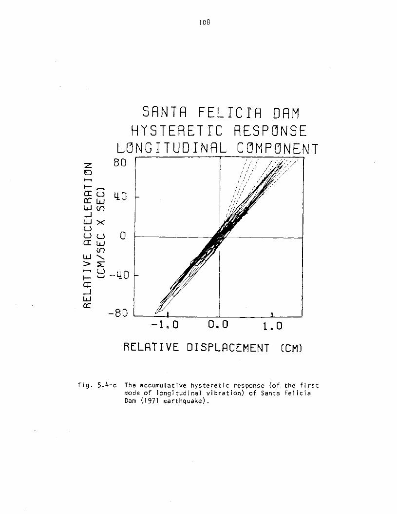
108
1. 0
RESPONSECOMP(jNENT
SANTA FELfCIA DAMHYSTERETfC
L~NGITUDINAL
80zo......t--~
a: u l!.0a:::wW(f)...JLUXUU U 0a:w
(f)
w">s:;:: ~ -l!.Oa:...J
~ -80 I'--_-&---_--LJ__---L-~0.0
RELRT I VE 0 I SPLRCEMENT (CM)
Fig. 5.4-c The accumulative hysteretic response (of the firstmode of longitudinal vibration) of Santa FeliciaDam (1971 earthquake).

109
analytical purposes, the R-O curves with R = 1.8 - 2.0, a = 1.7 - 1.75,
and C T = 800 to 1,200 psf (with Cl = 0.8) can be chosen, from Fig. 5.5 and fromI max
the normal ized curves of Fig. 5.6, to represent the relations for earth dam materials.
Taking G andmax T max from curves 1. 2, and 3 of Fig. 5.5, continuous
hyperbolic shearing stress-shearing strain curves (dotted curves) are deter-
mined (and are also shown in Fig. 5.5); the curves are given by
T = Y/[-Gl + f-]max max
The hyperbolic fit deviates considerably after the low-strain range,
indicating the R-O curves are a better match for the overall behavior.
V-2.2. Shear Moduli and Damping Factors for Santa Felicia Earth Dam
(5.6)
The secant shear modulus, G, for each hysteresis loop, can be obtained
by dividing Eq. 4.36 by Eq. 4.35. The relationship between the estimated shear
modulus and the dynamic shear strain is shown by the semi log plots of Fig. 5.7
for the first 25 secs of the 1971 earthquake and the first 6 sees of the 1976
earthquake. (Note that the number at each point corresponds to the time in
seconds at which the point was computed.) Again, it is apparent that the
modulus depends on the magnitude of the strain in the hysteresis loop.
The relationship between the estimated equivalent viscous damping factor
determined from the area of each hysteresis loop and the corresponding
h t · l't dare sh n' F'g 5 8 Wh',le there is a considerables ear-s raIn amp I u e ow In I •••
scatter in the data, most of the results fall within the dashed curves in
Figs. 5.7 and 5.8. The solid curve in each figure represents an estimate of
the mean behavior.
At higher strains, additional data on modulus values are needed; however,
approximate values for use in some types of response analyses are arrived at
by using the estimated values of the modulus at a very low strain level from

110
2000~----------- --,
curves0· 0G....= 3.85 X I~PSIcurves ® .,0G....= 4·OOx lOps'
0f C,T_.= 800 p.'Curve 1 • = 2.00
f,;\ C,T_.:I000 ps'o .. 2.00t3'! c.T...= 1000p,'I..:;J.. \.80
Q c.T...=1200 p.'1;:,).. 1.90
For all curvesll= 1.75c, = 0.6
Ramberg -Osgood Equat ion
T = PGmu A, +al~,R'JV L C,T",..
Hyperbolic Equation
/~ 1 F~T = P _+_Gm•• T....
SANTA FELICIA EARTH DAM
i> SAN FERNANDO E.Q OF FEB 9, 1971 (M =63)• SOUTHERN CALIFORNIA E.Q OF APRIL
L8, 1976 (MC4.7)
LONGITUDINAL COMPONENT(FIRST MODE)1500
-:.-"-£!1000
lI)lI)ILlex:l-ll)
ex:eXILl
500rlI)
0~-.4--_.....1-_~_--I-._~"":'----l__.L.-_...1--_...l--_-l-_--'-_-l
o 2 4 6 8 10 12
SHEAR STRAIN (PERCENT) X 10-2
Fig. 5.5 Estimated shear strain and srreS5 for each hysteresis loop andfit of Ramberg-Osgood and hyperbolic curves to earthquake data.
I O~------------------------I
0.8
.. IJ0
fi 0.6ex:
lI)lI)ILlex: 0.4l-ll)
ex:eXw:z:VI
0.2
I":\f C,T.....= 800 pa'Curve\!.l 11= 2.00
f';;\ . c,T.....=IOOO palo 11= 2.00(j\f C,T_.= 100Qpa'\J 11= 1.80
Q C,T_.= 1200 psI
V 11= 1.90
For all curves
il= 1.75c, = 0.6
curvesG) & 0,a = 3.85 x 10 pa'
m" f';;\ f.i\curves 0 &,0a :; 4.00X 10pa'
m"
SANTA FELICIA EARTH DAM
LONGITUDINAL COMPONENT
Ramberg-Osgood Equation
or :; I'a..... I, + 111_'11"'JV L C,'f•••
2 3
SHEAR STRAIN RATIO rGm•• / T.....
Fig. 5.6 Normalized shear strain-shear stress curves (RambergOsgood Models).

111
7r--------------------------,
6
SANTA FELICIA EARTH DAM
o SAN FERNANDO E.Q OF FEB 9, 1971 {ML6.3l_ SWTHERN CALIFORNIA E.Q. OF APRIL 8, 1976 {Ml 4.7l
300
5 L(1,IGITUDINAL COMPONENT(FIRST MOOEl
250
4QxCIl:::l
~ 3co~
~~ 2CIl
200 _0Q.
Ul:::loJ
150 :::l
8~
a:.q
100w:I:Ul
50
0l.:--::-- ~_----~:__-----L...,__-----l10.4 10-' 10-1 10·'
SHEAR STRAIN (PERCENT)
Fi g. 5.7 Estimated shear moduli and corresponding dynamic shear strains(evaluated from hysteretic response of two earthquakes).
35 r------------------------.,
30
SANTA FELICIA EARTH DAM
o SAN FERNANDO E.Q. OF FEB 9, 1971 (M~6.3l
- SOUTHERN CALIFORNIA E.Q. OF APRIL 8, 1976 (ML"4.7l
10.1 10-'SHEAR STRAIN (PERCENT)
10·'
LONGITUDINAL COMPONENT(FIRST MODEl
8 /o 7"o 12 *0 9 7/11 0 1
/06 0/VALUES MEAS~D FROM 19,/ ~AA/FULL-SCALE TESTS !JJ.."P "r:jP 6
/
,,~6 5 14 '" ~5./...... 24' 0 P" (;) 6
__- ....·23 . ",'"2_ 1 22 . 18' ",;,'" 4
4 ...~ 03- _",-- 25---10'"
5
25
~w(,)a:wQ. 200
~a:
~ 15ii:~.qc
10
Fig. 5.8 Estimated damping factors and corresponding dynamic shearstrains (evaluated from hysteretic response of two earthquakes).

112
the forced and ambient vibration tests (3) as well as from the in-situ geo
physical tests (1,4), with the aid of the analytical models, as indicated
in Figs. 5.7 and 5.8. Both figures indicate that the dynamic properties of
the dam1s constituent material estimated from low-strain full-scale tests
are consistent with those determined from the relatively larger strains induced
by the two earthquakes (if one extrapolates the data of Figs. 5.7 and 5.8 to
the low-strain range). Furthermore, the low-strain analytical models in
which the elastic moduli of the dam material vary along the depth are the most
appropriate representations for predicting the dynamic properties, as indicated
Q, 1 2 1by Fig. 5.7 (where an average value of the cases where m= 5' 5' 2' 1 would be
a reasonable extension of the earthquake data, which also were based on an
average value of various models (as shown by Table 5.1)).
From the R-O curve (Eq. 5.5) the decrease in secant modulus, G(= T/Y) ,
with an increase in shearing stress ratio, TIT ,i smax
G = Gmax
Figure 5.9 shows the decrease of secant modulus, G, with strain, Y,
for the same special values of Gmax ' a, CITmax ' and R of curves 1,2,
3, and 4 of Fig. 5.5; shown also on Fig. 5.9 are the data of Fig. 5.7. The R-O
curves match both the estimated earthquake results and the results of low-
strain full-scale tests very well indicating both the reliability of the
developed longitudinal analytical models in predicting earthquake induced
stresses and strains (in the first mode) and the appl icability of the R-O
curves to represent the stiffness relations for earth dams. The normal ized curves
of the shear modul us (wi th n~spect to
Fig. 5.10.
G ) versus shear strain are shown inmax
Finally, the damping factors are evaluated, by integration, from the

113
For all curves(H 1.75C, = 0.6
clJrvesG) a 0,G...? 3.85)( 10,.'cIJrves0 a,0G...? 4.00)( 10 po'
C r.\f C,T_.= 800 p.,urveo..!J • = 2.00
12' c,T_.=IOOO po'\.V • = 2.00Ij\f C,T_.= 1000 ,.,'..::.J.. 1.80
f4\ C,T...= 1200 p.'~ .. 1.90
LONGITUDINAL COMPONENT(FIRST MODEl
•
"""... '. "" ". ",,~.... ""l8 .... \." .....•.. \
• "~$. \~" "• ~18..."
\ \. ~
$.. C8' '\..
"" ,.'~
SANTA FELICIA EARTH DAM
o SAN FERNANDO E.Q. OF FEB 9,1971 (MC6.3l• SOUTHERN CALIFORNIA E.Q. OF APRIL 8,1976(MC4.7)
Ramberg-OsgoOd Equation
4
2
oI 10
SHEAR STRAIN (PERCENT)
Fig. 5.9 Fit of Ramberg-Osgood curves to estimated values of straindependent shear moduli.
~.6
• ~.!l•E
"........"o~0::
en~
~ t'J.1i8~
iw::r:en (L 2
I':'\f C,T_.= 800 pi'Curve\!.! A:: 2.00
f2\ c,T...=IOOO PI'\:.J R= 2.00
f3\f C,T_.= ICOOpl'\::.J A= '.BOQ c,T_.:: 1200 PII
\:::.J A= 1.90
curvesG) & 0,G
M..: 3.85 X 10pI'
curves® &,0GMI.= 4.00)( 10 pll
SANTA FELICIA EARTH DAM
LOOGITUDtNAL COMPONENT
Ramberg -Osgood Equation
T : VG_ IL •al_T I"'J1 L C,T•••
For all curvesa= 1.75c,: 0.6
aL- .J..- ...J....- ...!- .....L. --J
t:l.OCl1 Cl.Ol ILl HI HIO
Fig. 5.10 Normalized shear strain-shear modulus (Ramberg-OsgoodModels).

114
R-O curves (where the area of the hysteresis loop form~d is a measure of
the hysteretic damping occurring in the dam materials) for the same special
conditions of curves 1,2, 3, and 4 of Fig. 5.5. The results are shown on Fig. 5.11
which displays the earthquake data (of Fig. 5.8) as well. The R-O curves,
which represent the best fit of the three sets of data of Figs. 5.5, 5.7, and 5.8
represent a lower bound of the earthquake damping data. The normalized version of
Fig. 5.11 is shown in Fig. 5.12.
V-2.3. Axial Strains and Stresses of Santa Felicia Dam
Unfortunately, there were no acce1erographs on the dam crest near its
ends (where the maximum axial strains and stresses occur); only two siesmo
scopes were located on the east and west abutments (not on the crest) of the
dam. The existence of such acce1erographs would be very helpful in assessing
the amplitude dependence of axial strains and stresses and also in explaining,
more accurately, the transverse crack caused by the 1971 earthquake. However,
the standard response spectra technique is util ized to quantify the order of
magnitude of these axial stresses and strains. Table 5.2 shows the values of
these strains and stresses resulting from the spectral peaks of the recorded
ground motions (at the base of the dam) during the two earthquakes, assuming
uniform input ground motions.
It is necessary to very carefully compare the stresses given in Table 5.2
with the tensile strength of the dam material in order to assess or predict
a crack in a dam. As mentioned previously, the occurrence of cracks is in
consequence not only of the transient state of stress of the dam during an
earthquake, but also of the state of stress before an earthquake. It is
also necessary to further investigate the mechanism of cracking in earth fill
material under the action of irregular loads.

115
10
For all curvesa= 1.75c,: 0.6
SANTA FELICIA EARTH DAM
~ SAN FERNANDO E.Q. OF FEB 9, 1971 (Me 6.31• SOUTHERN CALIFORNIA E.Q. OF APRIL 8,1976(Mc=4.71
LONGITUDINAL COMPONENT(FIRST MODE)
Ramberg -Osgood Equat Ion
5
C I7\f C,T....=800 pilurve\!.l II::: 2.00
f2\ C,T.... :::IOoo pilt:'\ r:\ \=.J 11= 2.00curves \.!.J & ~6 ~ tj\fC,T_.: 1000PIIGm..: 3.85 X 10piI ~ \::.J II::: '-80
curves ® & 6 ® f4\ c, T_.: 1200 PIIGm..: 4.oox 10PII '2J II::: 1.90
0L.:=-....;.~~~~__~__.l--_~.J..-_--.J
10-5 10-4
15
10
25
30
SHEAR STRAIN (PERCENT)
Fig. 5.11 Fit of Ramberg-Osgood curves to estimated values of straindependent damping factors.
3C,.....--------------------------------"'
28
Q 16
~Q:
(!) 12;o 8
SANTA FELICIA EARTH DAM
LONGITUDINAL COMPONENT
For all curvesa= 1.75C,: 0·6
Ramberg -Osgood Equation
T ::: VG_A1 +al-T I"'JV L C,T•••
C t:'\f C,T.... ::: BOO pi'urve\!.l II::: 2.00
f2\ C,T....=IOoo pi'I..::.J 11= 2.00
I3\f C,T_.::: 1000piI\::.J II: '·8014\ C,T_.= 1200 pil @'2J II: 1.90 ,
curvesG) & 0•G
III••= 3.85 X 10pI'
curves@ &.0Gill..: 4·OOx 10 ...'
" L ~~E=__...I..____...L___~_ __.JO.IHlC1 C.M1 IL01 ILl U! loe
SHEAR STRAIN RATIO
Fig. 5.12 Normalized shear strain-damping ratio (Ramberg-Osgood Models).

116
Table 5.2
Estimated Axial Strains and Stresses in Santa Fel icia DamUsing Response Spectra Technique
I ASSUMED DAMPING RATIO (PERCENT)IPARAMETE~
2% 5% 10%,
1. 1971 San Fernando Earthquake t TIl = 0.74 sec,Sd 1.65 em 1.27 em 1.02 em
S 98.0 em/sec2 78.4 em/sec2 63.7 em/sec2a
£1 tIl max 0.0458 (percent) 0.0352 (percent) 0.0282 (percent)
°1 t 1Imax 1t 504.7 psf 1t 203.8 psf 978.1 psf
2. 1976 Earthquake T1 1 = 0.79 sect
Sd 0.71 em 0.41 em 0.33 em
S 39.2 em/sec2 27.4 em/sec2 19.6 em/sec2a
£1 t l lmax 0.0197 (percent) 0.0114 (percent) 0.0092 (percent)
° 1,1 Imax 601.9 psf 420.7 psf 301.0 psf
117
CONCLUSIONS
The analytical models developed here and the data presented will provide
information of practical as well as academic significance about the dynamic
characteristics of earth dams vibrating in a direction parallel to their longi
tudinal axis. Real earthquake observations of earth dams and experimental
results have confirmed that the models which take into account the effect
of variation with depth of both the shear modulus and the modulus of elasticity
of the dam material provide the most appropriate representation for predicting
the dynamic characteristics in the longitudinal direction. These
models are shown to be accurate enough so that they can be used for estimating
earthquake induced longitudinal strains and stresses (both shear and normal
or axial) on earth dams.
In addition t the formula and curves presented here will enable the determina
tion t for many practical purposes, of the dynamic strains and stresses (both shear
and normal) induced in a wide class of earth dams by the longitudinal component
of earthquake ground motions. Reasonable estimates of the
dynamic stress-strain curves (nonlinear strain-softening type) and the strain
dependent elastic modul i and damping for earth dam materials can be obtained
by using the proposed dynamic analysis procedure t earthquake records (on and
in the vicinity of dams)t and the adoption of the Ramberg-Osgood-type curves.
These estimates would be useful for any study of the dam1s earthquake-response
characteristics; in addition, the variation of material properties with depth
should be taken into account for any real istic dynamics study. Figures 5.5 to
5.12 should provide a good guide to the material properties in the dynamic
analysis of any earth dam composed predominantly of rolled-fill, essentially
cohesionless material, with or without a relatively thin core. Despite the
value of this studYt however t further research to accurately assess and
mitigate potentially adverse effects of seismic shaking on earth dams is
needed.


118
REFERENCES
I. Abdel-Ghaffar, A. M., and Scott, R. F., "An Investigation of the DynamicCharacteristics of an Earth Dam," EERL-78-02, Earthquake EngineeringResearch Laboratory, California Institute of Technology, Pasadena, CA,August 1978.
2. Abdel-Ghaffar, Ahmed M., "Engineering Data and Analyses of the Whittier,California Earthquake of January 1, 1976," EERL-77-05, EarthquakeEngineering Research Laboratory, Cal ifornia Institute of Technology,Pasadena, CA, November 1977.
3. Abdel-Ghaffar, A. t~., Scott, R. F. and Craig, M. M., "Full-Scale Experimental Investigation of a Hodern Earth Dam,I' EERL-80-01, EarthquakeEngineering Research Laboratory, California Institute of Technology,Pasadena, CA, February 1980.
4. Abdel-Ghaffar, Ahmed M., and Scott, Ronald F., "Analysis of Earth DamResponse to Earthquakes," Journal of the Geotechnical EngineeringDivision, ASCE, Vol. 105, No. GTI2, Proc. Paper 15033, December 1979,pp.1379-1404.
5. Abdel-Ghaffar, Ahmed M. and Koh, Aik-Siong, IILongitudinal Vibration ofNonhomogeneous Earth Dams," to appear in the International Journal ofEarthquake Engineering and Structural Dynamics, 1981.
6. Abdel-Ghaffar, Ahmed M., and Scott, Ronald F., "Shear Moduli and DampingFactors of Earth Dams,'l Journal of the Geotechnical Engineering Division,ASCE, Vol. 105, No. GTI2, Proc. Paper 15034, December 1979, pp. 1405-1426.
7. Abdel-Ghaffar, Ahmed M., and Scott, Ronald F., "Vibration Tests of aFull-Scale Earth Dam," Journal of the Geotechnical Engineering Division,ASCE, Vol. 107, No. GT3, March 1981.
8. Abdel-Ghaffar, Ahmed M., and Scott, Ronald F., "Comparative Study ofDynamic Response of an Earth Dam,1I Journal of the Geotechnical EngineeringDivision, ASCE, Vol. 107, No. GT3, March 1981.
9. Ambraseys, N. N., "On the Shear Response of a Two-Dimensional WedgeSubjected to an Arbitrary Disturbance,1I Bulletin of the SeismologicalSociety of America, Vol. 50, No.1, January 1960, pp. 45-56.
10. Ambraseys, N. fL, liOn the Seismic Behavior of Earth Dams," Proceedings ofthe Second World Conference on Earthquake Engineering, Japan, 1960,Vol. I, pp. 331-354.
11. Chopra, A. K., "Earthquake Response of Earth Dams,'1 Journal of SoilMechanics and Foundations Division, ASCE, Vol. 93, No. SM2, 1967.
12. Chopra, A. K., Dibaj, M., Clough, R. W., Penzin, J., and Seed, H. B.,IIEarthquake Analysis of Earth Dams,1I Proceedings, Fourth World Conferenceon Earthquake Engineering, Santiago, Chi Ie, January 1969.

119
13. Clough, R. W. and Chopra, A. K., IIEarthquake Stress Analysis in EarthDams,1I Journal of Engineering Mechanics Division, ASCE, Vol. 92,No. EM2, Apri 1 1966, pp. 198-211.
14. Clough, R. W. and Woodward, R. J., IIAnalysis of Embankment Stressesand Deformations,11 Journal of Soil Mechanics and Foundations Division,ASCE, Vol. 93, SM4, pp. 529-549, 1967.
15. Duke, C. M., IIFoundation and Earth Structures in Earthquakes,lI Proceedings of the Second World Conference on Earthquake Engineering, Japan,1960, Vol. 1, pp. 435-456.
16. Gazetas, G., and Abdel-Ghaffar, A. M., IIEarth Dam Characteristics fromFull-Scale Vibrations,1I Proceedings of the X International Conferenceon Soil Mechanics and Foundation Engineering, Stockholm, Sweden,June 15- 19, 1981.
17. Gazetas, G., '13-Dimensional Lateral and Longitudinal Seismic Stabilityof Earth and Rockfull Dams," Proceedings of the Seventh World Conference on Earthquake Engineering, Istanbul, Turkey, September 1980.
18. Hatanaka, M., "Fundamental Consideration on the Earthquake ResistantProperties of the Earth Dam,1I Bulletin No. 11 Disaster PreventionResearch Institute, Kyoto University, Japan, 1955.
19. Hatano, T. and Watanabe, H., IISe ismic Analysis of Earth Dams,1I Proc.4th World conference on Earthquake Engineering, Santiago, Chile, 1969.
20. Ishizaki, H. and Hatakeyama, N., "Consideration on the Dynamical Behaviorsof Earth Dams," Disaster Prevention Res. Inst., Kyoto University,Bulletin No. 52, 1962.
21. Keight1ey, W.O., "Vibrationa1 Characteristics of an Earth Dam,1IBulletin of the Seismological Society of America, Vol. 56, No.6,December 1966, pp. 1207-1226.
22. Makdisi, F. I. and Seed, H. B., IISimpl ified Procedure for EstimatingDam and Embankment Earthquake Induced Deformations,ll Journal ofGeotechnical Engineering Division, ASCE, Vol. 104, No. GT7, July 1978,pp.850-367.
23. Martin, G. R., liThe Response of Earth Dams to Earthquakes,1I thesispresented to the University of Cal ifornia, At Berkeley, CA, in 1965, inpartial fulfillment of the requirements for the degree of Doctor ofPhilosophy.
24. Medvedev, S. and Sinitsyn, A., "Se ismic Effects on Earth Fill Dams,1IProceeding 3rd World Conference on Earthquake Engineering, New Zealand,1965, Paper IV/M/18.
25. Minami, I., liOn Vibration Characteristics of Fill Dams in Earthquakes,'1Proceedings 4th World Conference on Earthquake Engineering, 1968,Santiago, Chile, paper A-5, pp. 101-115.

120
26. Mori, Y. and Kawakami, F. "Dynamic Properties of the Ainono Earth Damand the Ushino Rockfil1 Dam," Proceedings, Jap. Soc. Civ. Eng.,No. 240,1975, pp. 129-136.
27. Seed, H. B. and Idriss, I. B., "Soil Moduli and Damping Factors forDynamic Response Analysis,11 Report No. EERC 70-10, Earthquake EngineeringResearch Center, University of California, Berkeley, CA, December, 1970.
28. Seed, H. 13., IIA Method for Earthquake-Resistant Design of Earth Dams,"Journal of the Soil Mechanics and Foundations Division, ASCE, Vol. 92,No. SM1, January 1966, pp. 1l1-41.
29. Seed, B. H., Makdisi, F. I. and DeAlba, P., "Performance of Earth DamsDuring Earthquakes," Journal of the Geotechnical Engineering Division,ASCE, Vol. 104, No. GT7, July 1978, pp. 968-994.
30. Sherard, J. L., Woodward, R. J., Gizienski, S. F. and Clevenger, W. A.,Earth and Earth-Rock Dams, John Wiley & Sons, Inc., New York, 1963.
31. Richart, F. E., IIFoundation Vibr:ations," Journal of the Soil Mechanicsand Foundations Division, Proceedings ASCE, August 1960, pp. 1-34.
32. Richart, F. E., Jr., and Wylie, E. B., "Influence of Dynamic SoilPropert i es on Response of So i 1 Masses, II Structura 1 and Geotechn i ca 1Mechanics, a volume honoring Nathan M. Newmark, Editor W. J. Hall,Prentice-Hall, Englewood Cl iffs, NJ, pp. 141-162, 1977.


121
APPENDIX A
STANDARD (UNFILTERED) EARTHQUAKE
RECORDS OF SANTA FELICIA DAM
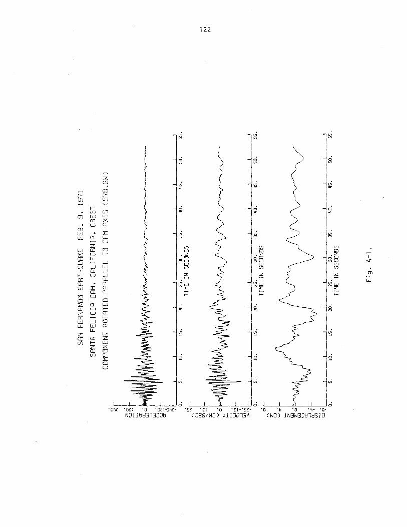
SAN
FERN
ANDO
EART
HQUR
KEFE
B.
9.19
71
SRNT
RFE
LIC
IRDR
M.
CRLI
FORN
IA.
CRES
T
COM
PONE
NTRO
TATE
DPR
RRLL
ELTO
DRM
RXIS
(S78
.GW
)
5.
10.
15.
II
II
II
20.
25.
30.
35.
40.
45.
50.
55.
TIM
EIN
SECO
NDS
~.)
t.,)
5.
10
.15
.20
.25
.30
.35
.TI
ME
INSE
COND
S40
.45
.50
.
II
--+--~IO~.
15.
I...L
.-_
lI
II
I20
.25
.30
.35
.40
.45
.50
.TI
ME
INSE
COND
S
Fig
.A
-I.
.J 55.

SRN
FERN
RNDO
ERRT
HQUR
KEFE
B.
9.
1971
SRNT
AFE
LIC
IRDR
M.
CR
LIFO
RN
IR.
OUTL
ETW
ORKS
COM
PONE
NTRO
TRTE
DPR
RRLL
ELTO
DRM
RXIS
(S78
.GW
)o =" N
O.
5.
10.
15.
20.
25.
30.
35.
lIO.
lI5.
50.
55.
1Il_
TIM
EIN
SECO
NDS
~
N
U w,
({)~I
N,- L
vJ
U ~ >- ~ .......
u~
0-
-1
'w~
>N
I
O.
5.
10.
15.
20.
25.
30.
35.
lIO.
liS
.50
.55
.
CD-
TIM
EIN
SECO
NDS
~ L U ~="
~ z W LO
uJ
U a: -1
'Q..~
({) .......
Gop
iI
II
II
II
II
I-.
---J
0,
5.
10.
IS.
20.
25.
30.
35.
110.
liS
,50
.55
.TI
ME
INSE
COND
S
Fig
.A
-2.

SRN
FERN
RNDO
ERRT
HQUR
KEFE
B.
9.19
71SR
NTR
FELI
CIR
DRM
,CR
LIFO
RNIR
RELR
TIV
ER
CC
EL.,
VEL
.RN
DO
ISP.
OFCR
EST
W.R
.T.
RBUT
MEN
T
COM
PONE
NTRO
TRTE
DPR
RRLL
ELTO
DRM
RXIS
CS7
8.6W
)C
> ""N
~
15.
O.
ai
I a: 0:'
WO
...J
W.
Uo
u'"
a:;5
,II
~II
II
II
II
II
I,
O.
5.
10.
15.
20.
25.
30.
35.
~O.
~5.
50.
55.
TIM
EIN
SECO
NDS
'-/,
;HiII
IIJI/\
I\1> I- ~~
0
...J
'w.
.n>
':'1
II
II
II
II
II
I20
.25
.30
.35
.~O.
ijS
.50
.55
.TI
ME
INSE
COND
S
z,;
ON
.--,- In
,....'"
U w.
U1'"
,- L U ,.... L U ~~
I Z W LO
W u 5·
CL'r
U1 ......
a'?
II
II
II
II
II
II
O.
5.
10.
15.
20.
25.
30.
35.
~o
.ij
S.
50.
55.
TIM
EIN
SECO
NDS
Fig
.A
-3.

SANT
AFE
LICI
AO
AM
.CRE
ST.E
/Q~F
APRI
L8
1976
-072
1PS
TSA
NTA
FELI
CIA
DAM
.CRE
STCO
MS7
BW~PEAK
VA
LUES
:AC
CEL
=-3
1.ij
CM/S
EC/S
ECVE
LOCI
TY=
-1.9
CH/SE
CO
ISPL
=-1
.7eM
-35
z ~ ....u
..-.
~0
:....
..
~~o
~~
U 0:
~ !'-> ~J:1
2015
10TI
HE-
SECO
NDS
Fig
.A
-4.
5
35I
II
I
-2I
2I
II
I,
-2 20
> "-'
u...
.w
Utn
0I
II"V
!lAl
l~l\
J\Il
A..
I~
AA
./,
,..
\I
\E
>,)
ri
h7
,I
r,A
I)
\r
v*(
y"
..Jl
iLI
J > ..-. :z LIJ s: LIJ 5~O
n..
(fl .... CJ

SRNT
RFE
LIC
IROR
M.R
IGHT
RBUT
MEN
T.E/
QOF
RPRI
L8
1976
-072
1PS
T.
SRNT
RFE
LIC
IROR
M.R
IGHT
RBUT
MEN
TCa
MP.
S~~
oPE
RKV
RLU
ES:
RCCE
L==
-33.
6C
M/S
Ec/
SE
CVE
LOCI
TY=
1.0
CM
/SEC
D[S
PL=0
.2eM
N C'
10I
I
5TI
ME
-SE
COND
S
-35
z °u
.....
11.I
......
111
a::.....
a:u
0w
w..J
1I1
w.....
uJ:
Uu
a::
35 -2
>- ......
u...
..11
.IU
II1
00
.....
..JJ:
l.L
Ju>
2 -2.....
. z I.LJ
1:
I.LJ
U2
:0
a::
u..
JQ
.. en ~ 0
20
Fig
.A
-5

127
APPENDIX B
TABLES OF SHEAR STRAINS AND STRESSES
INDUCED BY THE TWO EARTHQUAKES

Tab
leB-
1
Est
imat
edL
ongi
tudi
nal
She
arS
trai
ns
and
Str
esse
san
dth
eC
orre
spon
ding
She
arM
odul
i
San
Fer
nand
oE
arth
quak
eo
fF
ebru
ary
9,
1971
Max
.Ace
el.
Max
.Dis
p1.
Ave
rage
Ave
rage
Slo
peE
quiv
.E
quiv
.E
quiv
alen
t(x
+w
)x
(x+
w)
Str
ess
Str
ain
She
arTi
me
9m
axm
ax(x
+w
)9
max
Per
cent
Mod
ulus
Cye
le(e
m/s
ee2 )
xem
9m
axm
axx
/see
2Ib
/ft2
(xl0
-2 )Ib
/ft2
(xI0
6 )N
o.S
ecs
+ve
-ve
+ve
-ve
cm/s
ee2
emm
ax1
0.0
-0.7
54
0.0
--0.
50--
40.0
0·50
50.0
47
1.2
2.04
2.31
I'".5
0-1
.a60
.052
.00.
800.
6656
.00.
7376
.765
9.8
2.93
2.21
.. 21
.0-2
.072
.872
.01.
001.
0072
.21.
0072
.284
9.9
4.08
2.08
32-
375
.075
.01.
081.
0875
.01.
0869
.488
3.5
4.40
2.01
43-
460
.5;6
0.0
0.91
0.92
60.3
0.92
65.9
710.
33.
751.
895
4-5
40.0
;46
.50.
630.
7543
.30.
6962
.851
0.1
2.81
1.82
65-
63l
l.0
;30.
()0.
470
.50
32.0
0.49
65.3
377
.02.
001.
897
6-6
.75
25.0
;27
.00.
250.
3526
.00.
3090
.030
6.3
1.22
2.51
r6
.5-7
.00.
400
.35
28.5
0.38
75.0
335.
71.
552.
17..
30.0
.27
.08
7-3
17.0
;17.
00.
150.
1817
.00.
1710
0.0
200.
30.
692.
90I
98-
914
.0i1
0.0
0.13
0.13
12.0
0.13
92.0
141
.40.
532.
6710
;9-1
021
.0·1
8.0
0.2
50.
2019
.5I
0.23
84.8
229.
70.
942.
4411
110-
1127
.5:2
5.0
0.38
0.33
26.3
0.36
73.1
309.
81.
472.
1112
jll-
12
28.0
:29
.00.
470.
4828
.50.
4859
.J~
335.
71.
961.
7113
.12-
1330
.029
.00.
460.
4629
.50.
4664
.134
5.9
1.89
1.83
!14
!13-
1419
.820
.00.
270.
2919
.90.
2871
.123
3.8
I.16
2.02
,15
14-1
512
.813
.00.
180.
1912
.90.
1967
.915
1.4
0.76
1.99
1615
-16
9.0
9.5
0.10
0.11
9.3
0.11
84.6
109.
60.
452.
4417
16-1
76
.68
.50
.07
10
.09
7.6
0.08
94.4
89.5
0.33
2.71
1817
-18
7.0
I7
.20.
080.
087.
I0.
0888
.883
.50.
332.
5319
18-1
912
.0;1
1.0
0.14
10.
1411
.50.
1482
.113
5.5
0.57
2.38
2019
-20
8.0
:8
.00
.10
10
.10
8.0
0.10
80.0
94.4
0.41
2.30
2120
-21
6.0
6.0
0.0
51
0.06
6.0
0.05
109.
070
.70.
203.
5422
21-2
24.
24
.20.
04O
.Oll
4.2
o.O
ll10
5.0
49.1
0.16
3.07
2322
-23
5.0
5.0
0.0
5i0
.05
5.0
0.05
100.
05~L9
0.20
2.95
2423
-24
8.4
8.4
0.09
i0.09
8.4
0.09
93.3
98.5
0.37
2.66
2524
-25
7.7
j7.
70.
080.
087.
70.
0896
.390
.80.
332.
75
tv 00
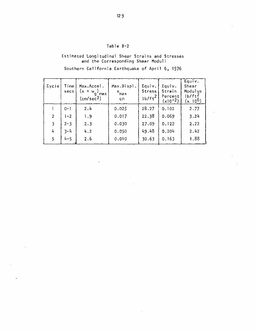
12 9
Table B-2
Estimated Longitudinal Shear Strains and Stressesand the Corresponding Shear Moduli
Southern California Earthquake of April 6, 1976
Equiv.Cycle Time Max.Accel. Max. Oi spl . Equiv. Equiv. Shear
sees (x + W ) x Stress Strain Modulusg max maxlb/ft2 Percent lb/ft 2
(cm/sec2) em (xI0-2) (x 106)
I 0-1 2.4 0.025 28.27 o. 102 2.77
2 1-2 1.9 0.017 22.38 0.069 3.24
3 2-3 2.3 0.030 27.09 0.122 2.22
4 3-4 4.2 0.050 49.48 0.204 2.42
5 4-5 2.6 0.040 30.63 0.163 1.88