Embed Size (px)
Citation preview

Beginner SWATTraining Manual
http://swatmodel.tamu.edu/
Soil & Water Assessment Tool

SecTion 1 ............................. 1SWaT OvervieW
SecTion 2 ............................. 21arcSWaT
arcgiS inTerface fOr SWaT
SecTion 3 ............................. 93SWaT calibraTiOn TechniqueS
SecTion 4 ............................. 107SWaT PublicaTiOnS
Table of Contents

SWAT overvieW
Section 1
1

2

Soil and WaterAssessment Tool
http://swatmodel.tamu.edu
R. [email protected] A&M University
Readily available input –Physically based
Comprehensive – Process Interactions Simulate Management
Model Philosophy
“Everything should be made as simple as possible. I have no interest in the laws of physics if they can’t be made simple”
Albert Einstein
Model Philosophy
3

ARS Modeling HistoryTime Line
CREAMS USLE (CLEAN WATER ACT) EPIC SWRRB SWAT
1960’s 1970’s 1980’s 1990’s
GLEAMS WEPP ANN AGNPS AGNPS
Environmental Models Maintained at Temple, TX
EPIC—Field Scale ALMANAC—Field ScaleAPEX—Farm Scale SWAT—Watershed Scale
Global Applications
HUMUSHUMER
HUMID
HUNCH
HUMAF
International SWAT Conferences
Hydrologic Unit Modeling for Global Eosystem/Environment
2001 Giessen, Germany2003 Bari, Italy2005 Zurich, Switzerland2006 Potsdam, Germany2007 Delft, Netherlands2008 Beijing, China2009 Chiang Mai, Thailand2009 Boulder, CO, USA2010 New Delhi, India2011 Toledo, Spain
4

Continuous TimeDaily Time StepOne Day Hundreds of Years
Distributed ParameterUnlimited Number of Subwatersheds
Comprehensive – Process Interactions Simulate Management
General Description
Example Configuration
Cells/Subwatersheds Hydrologic Response UnitsOutput from other Models Point Sources - Treatment Plants
Upland Processes
SWAT Watershed System
Channel/Flood PlainProcesses
5
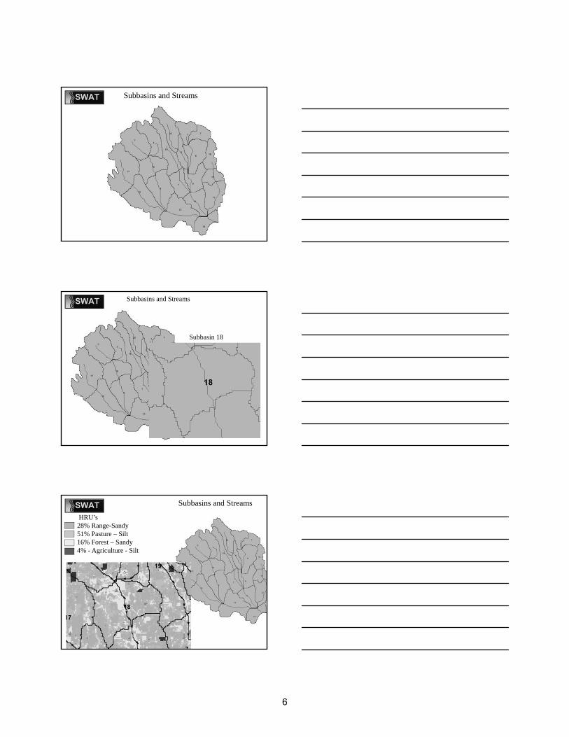
Subbasins and Streams
Subbasins and Streams
Subbasin 18
Subbasins and Streams
HRU’s28% Range-Sandy51% Pasture – Silt16% Forest – Sandy4% - Agriculture - Silt
6

Subbasins and Streams
Weather Hydrology Sedimentation Plant Growth Nutrient Cycling Pesticide Dynamics Management Bacteria
Upland Processes
Climate
• Weather– Precipitation – Air Temperature and Solar Radiation – Wind Speed – Relative Humidity
• Snow– Snow Cover – Snow Melt – Elevation Bands
• Soil Temperature
7
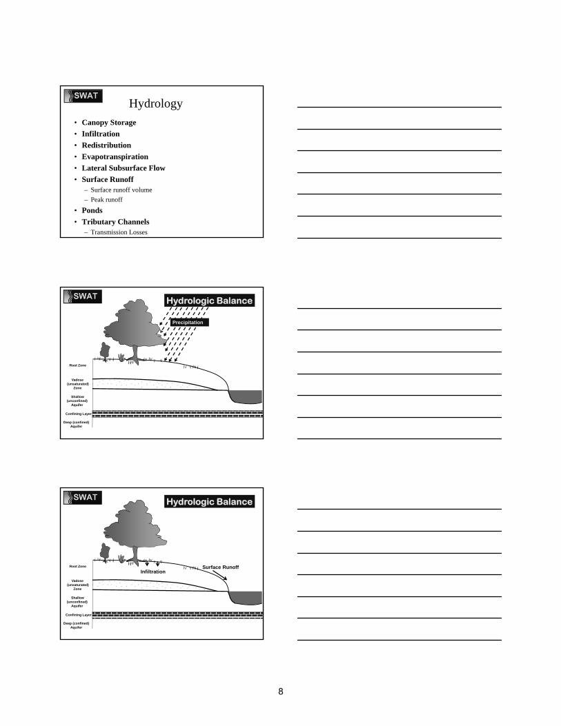
Hydrology• Canopy Storage
• Infiltration
• Redistribution
• Evapotranspiration
• Lateral Subsurface Flow
• Surface Runoff– Surface runoff volume – Peak runoff
• Ponds
• Tributary Channels– Transmission Losses
Root Zone
Shallow (unconfined)
Aquifer
Vadose(unsaturated)
Zone
Confining Layer
Deep (confined) Aquifer
Precipitation
Hydrologic Balance
Root Zone
Shallow (unconfined)
Aquifer
Vadose(unsaturated)
Zone
Confining Layer
Deep (confined) Aquifer
InfiltrationSurface Runoff
Hydrologic Balance
8
Root Zone
Shallow (unconfined)
Aquifer
Vadose(unsaturated)
Zone
Confining Layer
Deep (confined) Aquifer
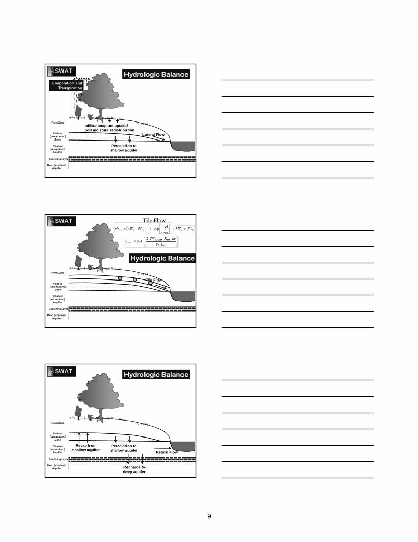
Evaporation and Transpiration
Infiltration/plant uptake/ Soil moisture redistribution
Lateral Flow
Percolation to shallow aquifer
Hydrologic Balance
Root Zone
Shallow (unconfined)
Aquifer
Vadose(unsaturated)
Zone
Confining Layer
Deep (confined) Aquifer
if
Tile Flow
Tile Flow
Hydrologic Balance
Root Zone
Shallow (unconfined)
Aquifer
Vadose(unsaturated)
Zone
Confining Layer
Deep (confined) Aquifer
Return Flow
Revap from shallow aquifer
Percolation to shallow aquifer
Recharge to deep aquifer
Hydrologic Balance
9
Root Zone
Shallow (unconfined)
Aquifer
Vadose(unsaturated)
Zone
Confining Layer
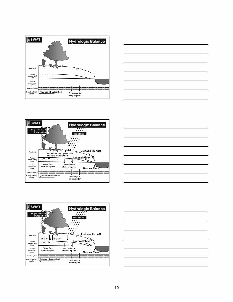
Deep (confined) Aquifer Recharge to
deep aquifer
Flow out of watershed
Hydrologic Balance
Root Zone
Shallow (unconfined)
Aquifer
Vadose(unsaturated)
Zone
Confining Layer
Deep (confined) Aquifer
Precipitation
Evaporation and Transpiration
Infiltration/plant uptake/ Soil moisture redistribution
Surface Runoff
Lateral Flow
Return Flow
Revap from shallow aquifer
Percolation to shallow aquifer
Recharge to deep aquifer
Flow out of watershed
Hydrologic Balance
Root Zone
Shallow (unconfined)
Aquifer
Vadose(unsaturated)
Zone
Confining Layer
Deep (confined) Aquifer
Precipitation
Evaporation and Transpiration
Infiltration/plant uptake
Surface Runoff
Lateral Flow
Return Flow
Revap from shallow aquifer
Percolation to shallow aquifer
Recharge to deep aquifer
Flow out of watershed
Hydrologic Balance
10
2 10840
0
9
6
3
12
Month
126
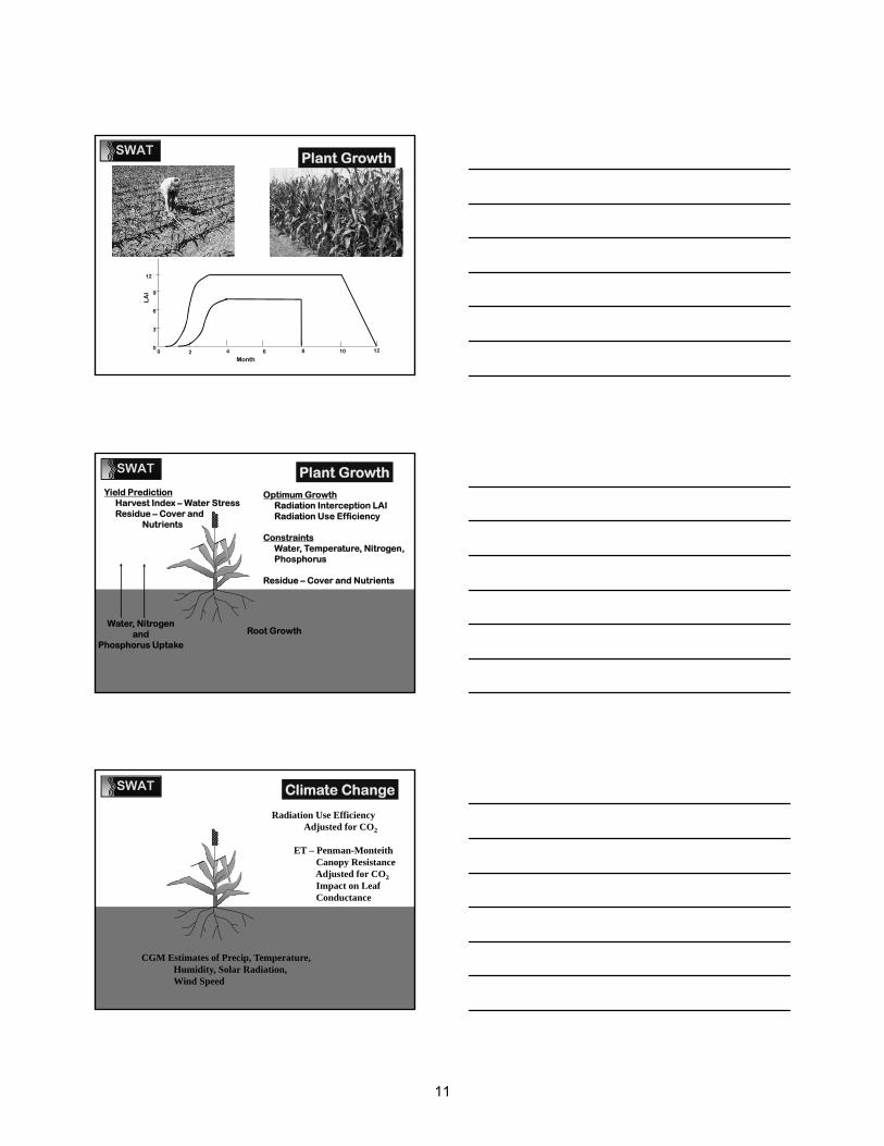
Plant Growth
Water, Nitrogenand
Phosphorus Uptake
Plant GrowthOptimum Growth
Radiation Interception LAIRadiation Use Efficiency
ConstraintsWater, Temperature, Nitrogen,Phosphorus
Residue – Cover and Nutrients
Yield PredictionHarvest Index – Water StressResidue – Cover and
Nutrients
Root Growth
Climate Change
Radiation Use EfficiencyAdjusted for CO2
ET – Penman-MonteithCanopy ResistanceAdjusted for CO2
Impact on LeafConductance
CGM Estimates of Precip, Temperature, Humidity, Solar Radiation,Wind Speed
11
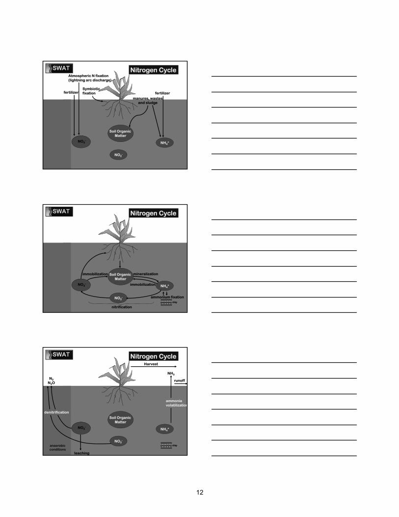
NO3- NH4
+
Soil Organic Matter
NO2-
manures, wastes and sludge
Symbiotic fixation
NO3-
Atmospheric N fixation (lightning arc discharge)
fertilizer fertilizer
Nitrogen Cycle
NO3- NH4
+
Soil Organic Matter
NO2- ammonium fixation
clay
mineralization
immobilization
nitrification
immobilization
NO3-
Nitrogen Cycle
NO3- NH4
+
Soil Organic Matter
NO2-
clay
NO3-
anaerobicconditions
N2 N2O
NH3
leaching
Harvest
Nitrogen Cycle
denitrification
ammonia volatilization
runoff
12
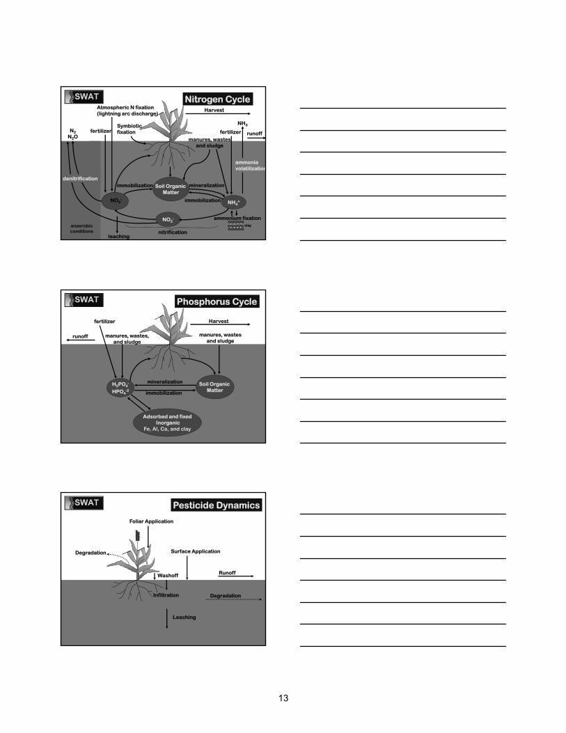
NO3- NH4
+
Soil Organic Matter
NO2-
manures, wastes and sludge
ammonium fixationclay
mineralization
immobilization
nitrification
immobilization
Symbiotic fixation
NO3-
anaerobicconditions
N2 N2O
NH3
Atmospheric N fixation (lightning arc discharge)
leaching
fertilizer fertilizer
Harvest
Nitrogen Cycle
denitrification
ammonia volatilization
runoff
Soil Organic Matter
H2PO4-
HPO4-2
manures, wastes and sludge
mineralization
immobilization
fertilizer Harvest
manures, wastes, and sludge
Adsorbed and fixedInorganic
Fe, Al, Ca, and clay
runoff
Phosphorus Cycle
Pesticide Dynamics
Foliar Application
Degradation
Washoff
Infiltration
Leaching
Runoff
Surface Application
Degradation
13

Crop Rotations Removal of Biomass as Harvest/
Conversion of Biomass to Residue Tillage / Biomixing of Soil Fertilizer Applications Grazing Pesticide Applications
Management
Management
Irrigation Subsurface (Tile) Drainage Water Impoundment (e.g. Rice)
Management
Urban AreasPervious/Impervious AreasStreet SweepingLawn Chemicals
Edge of Field Buffers
14

Channel Processes
Channel Processes Flood Routing
Variable StorageMuskingum
Transmission Losses, Evaporation
Sediment RoutingDegradation and deposition computed simultaneously
Channel Processes
Nutrients modified QUAL2E/WASP
Pesticide Toxic balance developed atUniversity of Colorado
15
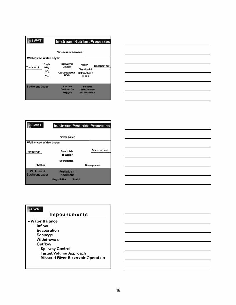
Well-mixed Water Layer
Sediment Layer
Atmospheric Aeration
Dissolved Oxygen
Benthic Demand for
Oxygen
Chlorophyll a Algae
Carbonaceous BOD
Org NNH4
NO2
NO3
Org P
Dissolved P
In-stream Nutrient Processes
Benthic Sink/Source for Nutrients
Transport outTransport in
Well-mixed Water Layer
Well-mixed Sediment Layer
Volatilization
Pesticide in Water
Pesticide in Sediment
Settling Resuspension
Burial
Degradation
In-stream Pesticide Processes
Transport in
Degradation
Transport out
Impoundments Water Balance
InflowEvaporationSeepageWithdrawalsOutflow
Spillway ControlTarget Volume ApproachMissouri River Reservoir Operation
16

Impoundments Nutrient Balance
Well-mixed SystemNitrogen & Phosphorus Loss Rates2 Settling Periods per Year
Pesticide BalanceWell-mixed SystemToxic balance developed at
University of Colorado
User Options• PET:
Penman-Monteith, Priestly-Taylor, or Hargreaves
• Runoff: Curve Number or Green & Ampt
• Channel Flow: Variable Storage Coefficient or Muskingham-
Cunge
• Channel Water Quality: QUAL2E On-Off Switch
More User Options• ARC GIS 9.3 or 10• Map Windows (Public Domain GIS)• SWAT-CUP (Calibration and Uncertainty Program• VIZSWAT (Output Vizualization)• Manuals in English, Spanish, Chinese, Korean• SWAT 2003, 2005, 2009, (2012)
17
SWAT StrengthsUpland Processes Comprehensive Hydrologic Balance Physically-Based Inputs Plant Growth – Rotations, Crop Yields Nutrient Cycling in Soil Land Management - BMP
Tillage, Irrigation, Fertilizer, Pesticides, Grazing, Rotations, Subsurface Drainage,Urban-Lawn Chemicals, Street Sweeping
SWAT StrengthsChannel Processes
Flexible Watershed Configuration Water Transfer—Irrigation Diversions Sediment Deposition/Scour Nutrient/Pesticide Transport Pond, Wetland and Reservoir Impacts
Collaborators
NOAA
EPAOffice of Science
and Technology
USDANatural Resources
Conservation Service
USDAAgricultural Research
Service
Texas A&MUniversity
Universities
18

Conclusions A product of over 45 years of USDA/Texas A&M
model development
Widely used for water quality, water supply, and climate change, carbon sequestration, and agricultural production assessments worldwide
•Over 1000’s SWAT users and 30 active developers worldwide
•Annual meetings alternate in Asia and Europe
The Endhttp://swatmodel.tamu.edu
19

20
Arc SWATArcgiS inTerfAce for SWAT
inTrOducTiOn
ObjecTiveS
WaTerShed delineaTiOn
hydrOlOgic reSPOnSe uniT definiTiOn
WriTe inPuT TableS fOr SWaTediT SWaT inPuT
SWaT SiMulaTiOn SeTuP
aPPendix: inSTalling arcSWaT
Section 2
21

22
R. Srinivasan, [email protected]
ArcSWAT
ArcGIS Interface for Soil and Water Assessment Tool (SWAT)
http://www.brc.tamus.edu/swat
R. Srinivasan
Blackland Research and Extension Center and Spatial Sciences Laboratory
Texas Agricultural Experiment Station
Texas A&M University
23
R. Srinivasan, [email protected] - 1 -
Table of Contents
Introduction ................................................................................................................................................ 1
Objectives .................................................................................................................................................. 1
Watershed Delineation ............................................................................................................................... 5
Hydrologic Response Unit Definition ........................................................................................................ 29
Write Input Tables for SWAT ................................................................................................................... 31
Edit SWAT Input ....................................................................................................................................... 35
SWAT Simulation Setup ........................................................................................................................... 56
Appendix: Installing ArcSWAT ................................................................................................................. 58
24

R. Srinivasan, [email protected] 1
Introduction The Soil and Water Assessment Tool (SWAT) is a physically-based continuous-event hydrologic model developed to predict the
impact of land management practices on water, sediment, and agricultural chemical yields in large, complex watersheds with varying
soils, land use, and management conditions over long periods of time. For simulation, a watershed is subdivided into a number of
homogenous subbasins (hydrologic response units or HRUs) having unique soil and land use properties. The input information for
each subbasin is grouped into categories of weather; unique areas of land cover, soil, and management within the subbasin;
ponds/reservoirs; groundwater; and the main channel or reach, draining the subbasin. The loading and movement of runoff,
sediment, nutrient and pesticide loadings to the main channel in each subbasin is simulated considering the effect of several physical
processes that influence the hydrology. For a detailed description of the capabilities of the SWAT, refer to Soil and Water
Assessment Tool User’s Manual, Version 2000 (Neitsch et al., 2002), published by the Agricultural Research Service and the Texas
Agricultural Experiment Station, Temple, Texas. The manual can also be downloaded from the SWAT Web site
(www.brc.tamus.edu/swat/swatdoc.html#new).
Objectives
The objectives of this exercise are to (1) setup a SWAT project and (2) familiarize with the capabilities of SWAT.
25

R. Srinivasan, [email protected] Texas A & M University 2
Figure 1 Extensions of ArcMap
Create a Project
ArcSWAT extension of ArcGIS 10 creates an ArcMap project file that contains links to your retrieved data and incorporates all
customized GIS functions into your ArcMap project file. The project file contains a customized ArcMap Graphical User Interface (GUI)
including menus, buttons, and tools. The major steps on how to create a SWAT project under then ArcMap environment are
introduced below:
Step 1. Start ArcMap. Under the Customize menu of ArcMap View,
click the Extensions button. You will see an extension entitled
“SWAT Project Manager” and “SWAT Watershed delineator”
under the extensions list (Figure 1). Turn on these two
extensions.
Step 2. Go to the Customize menu of ArcMap, hover the mouse over
the Toolbar button, a list of tools will appear. Click the
ArcSWAT tool, the main interface of ArcSWAT will open
26
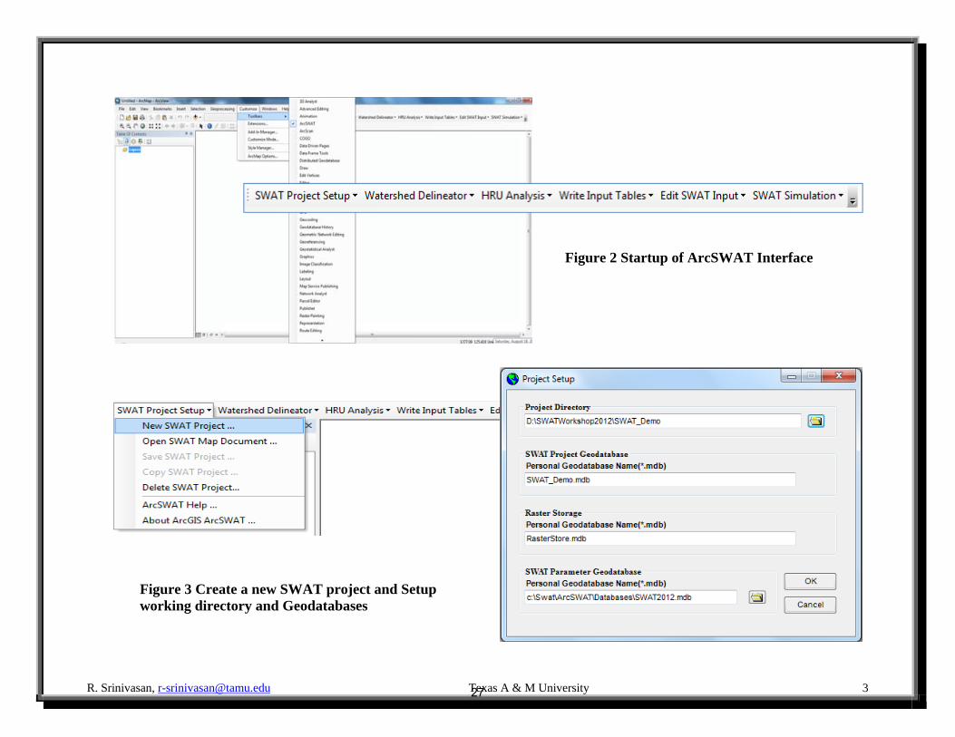
R. Srinivasan, [email protected] Texas A & M University 3
Figure 2 Startup of ArcSWAT Interface
Figure 3 Create a new SWAT project and Setup working directory and Geodatabases
27
R. Srinivasan, [email protected] Texas A & M University 4
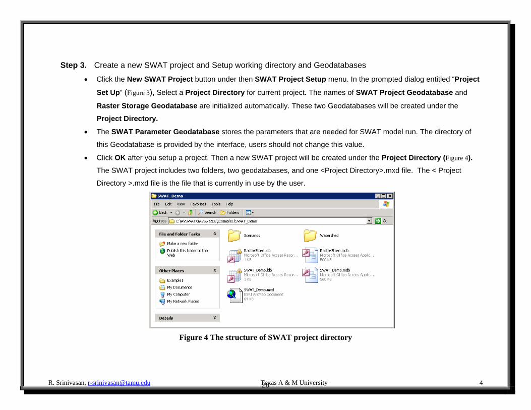
Step 3. Create a new SWAT project and Setup working directory and Geodatabases
Click the New SWAT Project button under then SWAT Project Setup menu. In the prompted dialog entitled “Project
Set Up” (Figure 3), Select a Project Directory for current project. The names of SWAT Project Geodatabase and
Raster Storage Geodatabase are initialized automatically. These two Geodatabases will be created under the
Project Directory.
The SWAT Parameter Geodatabase stores the parameters that are needed for SWAT model run. The directory of
this Geodatabase is provided by the interface, users should not change this value.
Click OK after you setup a project. Then a new SWAT project will be created under the Project Directory (Figure 4).
The SWAT project includes two folders, two geodatabases, and one <Project Directory>.mxd file. The < Project
Directory >.mxd file is the file that is currently in use by the user.
Figure 4 The structure of SWAT project directory
28
R. Srinivasan, [email protected] 5
Watershed Delineation
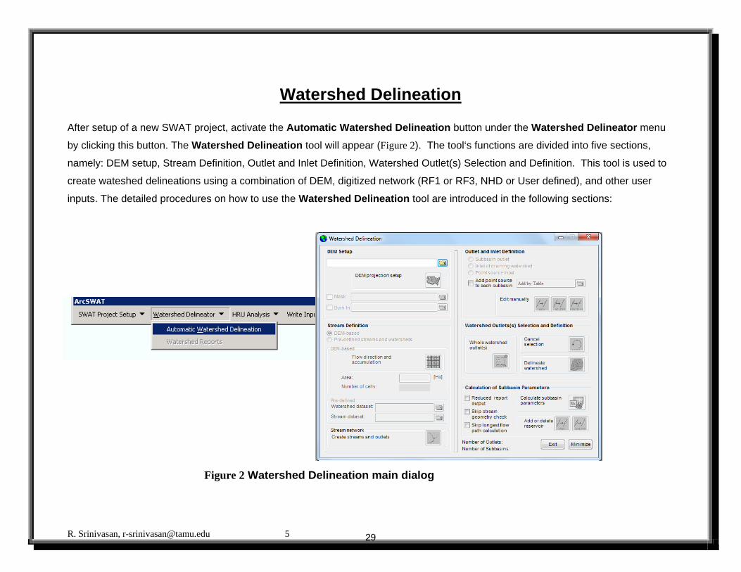
After setup of a new SWAT project, activate the Automatic Watershed Delineation button under the Watershed Delineator menu
by clicking this button. The Watershed Delineation tool will appear (Figure 2). The tool‘s functions are divided into five sections,
namely: DEM setup, Stream Definition, Outlet and Inlet Definition, Watershed Outlet(s) Selection and Definition. This tool is used to
create wateshed delineations using a combination of DEM, digitized network (RF1 or RF3, NHD or User defined), and other user
inputs. The detailed procedures on how to use the Watershed Delineation tool are introduced in the following sections:
Figure 2 Watershed Delineation main dialog
29
R. Srinivasan, [email protected] Texas A & M University 6
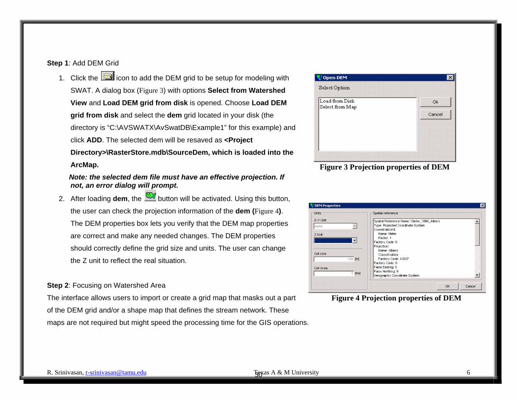
Step 1: Add DEM Grid
1. Click the icon to add the DEM grid to be setup for modeling with
SWAT. A dialog box (Figure 3) with options Select from Watershed
View and Load DEM grid from disk is opened. Choose Load DEM
grid from disk and select the dem grid located in your disk (the
directory is “C:\AVSWATX\AvSwatDB\Example1” for this example) and
click ADD. The selected dem will be resaved as <Project
Directory>\RasterStore.mdb\SourceDem, which is loaded into the
ArcMap.
Note: the selected dem file must have an effective projection. If not, an error dialog will prompt.
2. After loading dem, the button will be activated. Using this button,
the user can check the projection information of the dem (Figure 4).
The DEM properties box lets you verify that the DEM map properties
are correct and make any needed changes. The DEM properties
should correctly define the grid size and units. The user can change
the Z unit to reflect the real situation.
Step 2: Focusing on Watershed Area
The interface allows users to import or create a grid map that masks out a part
of the DEM grid and/or a shape map that defines the stream network. These
maps are not required but might speed the processing time for the GIS operations.
Figure 3 Projection properties of DEM
Figure 4 Projection properties of DEM
30
R. Srinivasan, [email protected] Texas A & M University 7
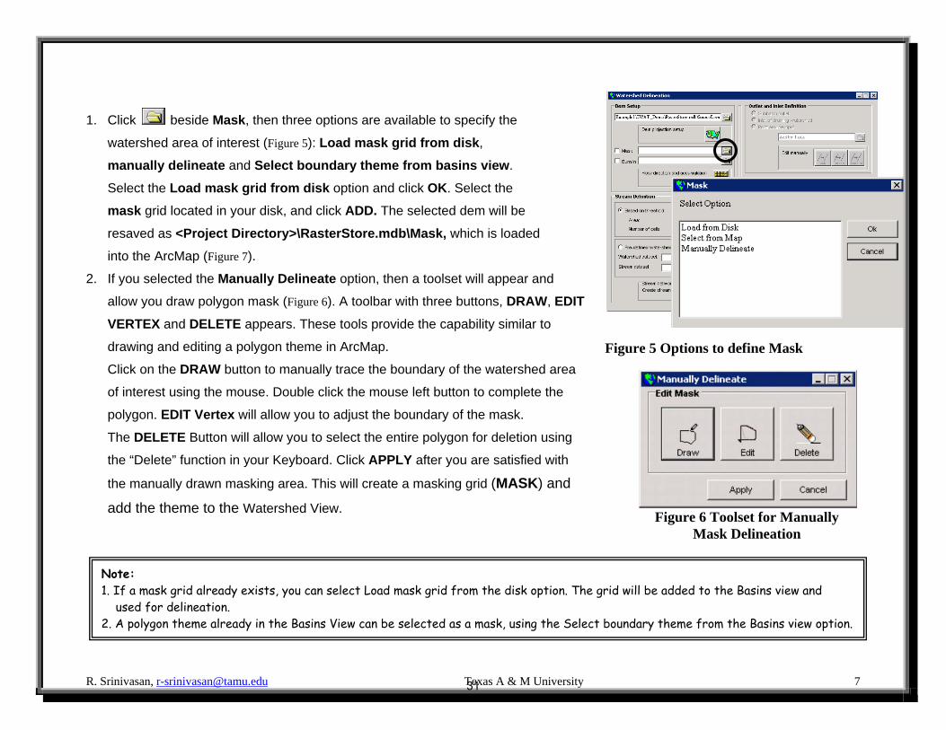
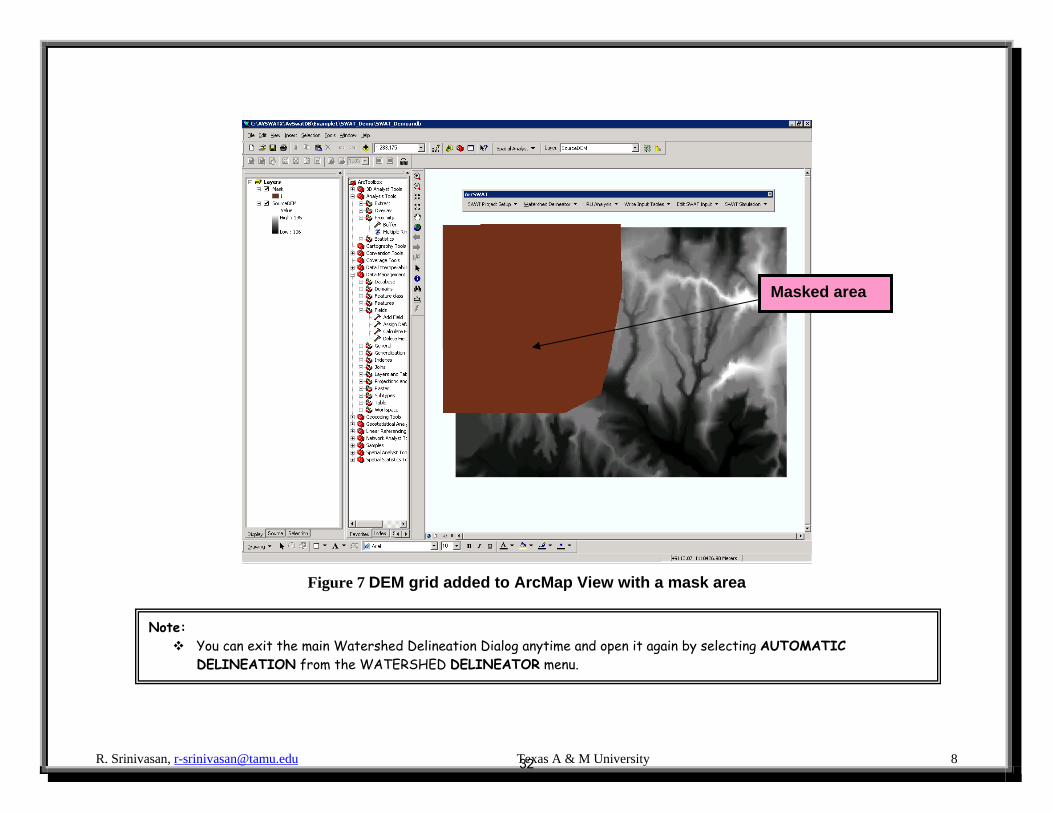
1. Click beside Mask, then three options are available to specify the
watershed area of interest (Figure 5): Load mask grid from disk,
manually delineate and Select boundary theme from basins view.
Select the Load mask grid from disk option and click OK. Select the
mask grid located in your disk, and click ADD. The selected dem will be
resaved as <Project Directory>\RasterStore.mdb\Mask, which is loaded
into the ArcMap (Figure 7).
2. If you selected the Manually Delineate option, then a toolset will appear and
allow you draw polygon mask (Figure 6). A toolbar with three buttons, DRAW, EDIT
VERTEX and DELETE appears. These tools provide the capability similar to
drawing and editing a polygon theme in ArcMap.
Click on the DRAW button to manually trace the boundary of the watershed area
of interest using the mouse. Double click the mouse left button to complete the
polygon. EDIT Vertex will allow you to adjust the boundary of the mask.
The DELETE Button will allow you to select the entire polygon for deletion using
the “Delete” function in your Keyboard. Click APPLY after you are satisfied with
the manually drawn masking area. This will create a masking grid (MASK) and
add the theme to the Watershed View.
Note: 1. If a mask grid already exists, you can select Load mask grid from the disk option. The grid will be added to the Basins view and used for delineation. 2. A polygon theme already in the Basins View can be selected as a mask, using the Select boundary theme from the Basins view option.
Figure 5 Options to define Mask
Figure 6 Toolset for Manually
Mask Delineation
31
R. Srinivasan, [email protected] Texas A & M University 8
Figure 7 DEM grid added to ArcMap View with a mask area
Note: You can exit the main Watershed Delineation Dialog anytime and open it again by selecting AUTOMATIC
DELINEATION from the WATERSHED DELINEATOR menu.
Masked area
32

R. Srinivasan, [email protected] Texas A & M University 9
Step 3: Burning in a stream network
A stream network theme such as Reach File (V1 or V3) or National Hydrography Dataset (NHD) can be superimposed onto the DEM
to define the location of the stream network.
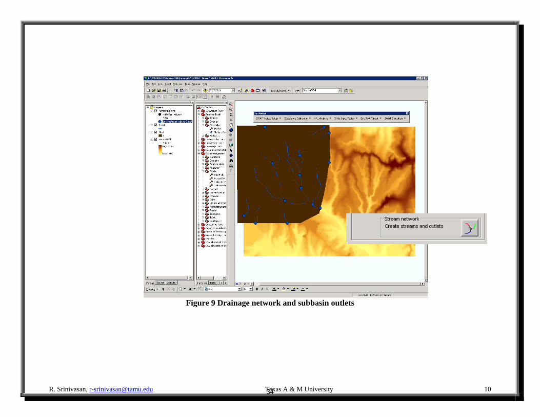
Step 4: Stream Definition
(Note: For the Stream Definition function of the Watershed Delineator, There are two ways to define the watershed and stream
network. In this section, the method based threshold area will be introduced, while another method based on pre-defined watershed
will be introduced in Appendix I.)
1. In order to use the threshold method to delineate the watershed and stream network, the Flow Direction and Accumulation
needs to be calculated by clicking the button. Stream definition defines both the stream network and subbasin outlets.
A minimum, maximum, and suggested sub watershed area (in hectares) is
shown in the drainage area box (Figure 8). You have the option of changing the
size of the subbasins within the specified range of values. This function plays
an important role in determining the detail of the stream network and the size and
number of subbasins created. The threshold area defines the drainage area
required to form the beginning of a stream.
2. After setting the threshold value of subbasin, then the user can delineate the stream network and outlets through clicking the
button. The drainage network and stream juncture points, used to define subbasin outlets, are displayed on the DEM
map grid (Error! Reference source not found.).
Note:
NHD is an enhanced stream network at the scale of 1:100,000. It is based on USGS Digital Line Graph (DLG) hydrography data integrated with reach-related information from the EPA River Reach File version 3 (RF3).
Figure 8 Threshold area for stream and subbasin definition
33
R. Srinivasan, [email protected] Texas A & M University 10
Figure 9 Drainage network and subbasin outlets
34
R. Srinivasan, [email protected] Texas A & M University 11
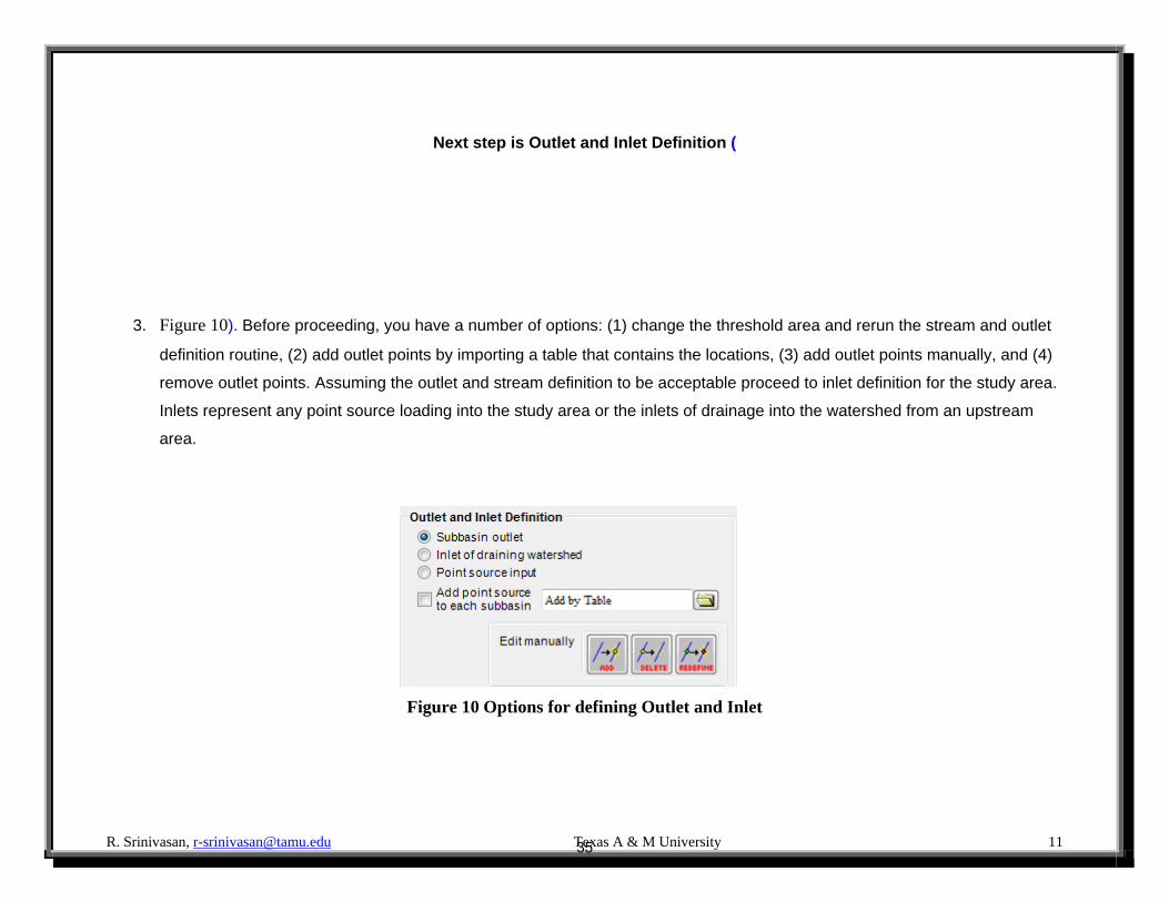
Next step is Outlet and Inlet Definition (
3. Figure 10). Before proceeding, you have a number of options: (1) change the threshold area and rerun the stream and outlet
definition routine, (2) add outlet points by importing a table that contains the locations, (3) add outlet points manually, and (4)
remove outlet points. Assuming the outlet and stream definition to be acceptable proceed to inlet definition for the study area.
Inlets represent any point source loading into the study area or the inlets of drainage into the watershed from an upstream
area.
Figure 10 Options for defining Outlet and Inlet
35

R. Srinivasan, [email protected] Texas A & M University 12
Note By specifying the threshold area, we define the stream network for networking. It means that a minimum number of cells are required to start delineating the stream. The minimum threshold area is for the entire watershed, not for each sub watersheds that are going to be delineated. The suggested area given in this window is the average are that could be used.
36
R. Srinivasan, [email protected] Texas A & M University 13
Step 5: Main Watershed Outlet(s) Selection and Definition
In this step the users will select one or more outlet locations to define the boundary of the main watershed.
Click on the SELECT button to choose the watershed outlet. Draw a box covering the desired outlet locations will set the main
Watershed Outlets. In this example, select 1 outlet at the downstream edge of the masked area (
1. Figure 11) and click the Delineate Watershed button . Select YES in the following dialog to continue with the delineation
of main watershed and subbasins. A prompt box will appear to announce completion of the watershed and subbasin
delineation.
2. The delineated watershed with subbasins will be added to the View. If the delineation is not satisfactory or if the user wants to
select a different outlet for the watershed, click on the Cancel Selection button and repeat.
Click on the Calculate Subbasin Parameters button to estimate the subbasin parameters. This function calculates basic watershed characteristics from the DEM and sub-watershed themes. It also assigns the necessary subbasin
identification. The results of the calculations are stored as additional fields in the streams and subbasins theme database files. Click OK to completion of watershed delineation dialog box.
3. Figure 12 shows the delineated watershed with subbasins.
4. Open the Reach or Watershed attribute tables to view the calculated characteristics.
37
R. Srinivasan, [email protected] Texas A & M University 14
** By holding the SHIFT key in your keyboard you can select more than one outlet. This feature allows adjacent watershed to be simulated at the same time using SWAT. Do not select an outlet at the upstream of another outlet. At least one outlet must be selected for delineation.
Selected outlet
38

R. Srinivasan, [email protected] Texas A & M University 15
Figure 11 Main watershed outlet selection
39
R. Srinivasan, [email protected] Texas A & M University 16
Figure 12 Delineated watershed and subbasins
40
R. Srinivasan, [email protected] Texas A & M University 17
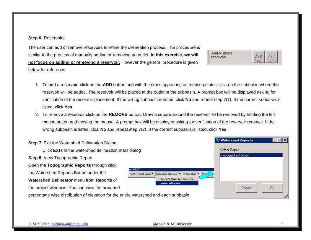
Step 6: Reservoirs The user can add or remove reservoirs to refine the delineation process. The procedure is
similar to the process of manually adding or removing an outlet. In this exercise, we will
not focus on adding or removing a reservoir. However the general procedure is given
below for reference.
1. To add a reservoir, click on the ADD button and with the cross appearing as mouse pointer, click on the subbasin where the
reservoir will be added. The reservoir will be placed at the outlet of the subbasin. A prompt box will be displayed asking for
verification of the reservoir placement. If the wrong subbasin is listed, click No and repeat step 7(1). If the correct subbasin is
listed, click Yes.
2. To remove a reservoir click on the REMOVE button. Draw a square around the reservoir to be removed by holding the left
mouse button and moving the mouse. A prompt box will be displayed asking for verification of the reservoir removal. If the
wrong subbasin is listed, click No and repeat step 7(2). If the correct subbasin is listed, click Yes.
Step 7: Exit the Watershed Delineation Dialog
Click EXIT in the watershed delineation main dialog
Step 8: View Topographic Report
Open the Topographic Reports through click
the Watershed Reports Button under the
Watershed Delineator menu from Reports of
the project windows. You can view the area and
percentage wise distribution of elevation for the entire watershed and each subbasin.
41
R. Srinivasan, [email protected] Texas A & M University 18
Land use, Soil and Slope Definition The Land Use, Soil and Slope Definition option in the HRU Analysis menu allows the user to specify the land use, soil and slope
themes that will be used for modeling using SWAT and NPSM. These themes are then used to determine the hydrologic response
unit (HRU) distribution in each sub-watershed.
Both NPSM and SWAT require land use data to determine the
area of each land category to be simulated within each subbasin.
In addition to land use information, SWAT relies on soil data to
determine the range of hydrologic characteristics found within
each subbasin. Land Use, Soil and Slope Definition option
guides the user through the process of specifying the data to be
used in the simulation and of ensuring that those data are in the
appropriate format. In particular, the option allows the user to
select land use or soil data that are in either shape or grid
format. Shapefiles are automatically converted to grid, the
format required by ArcGIS to calculate land use and soil
distributions within the subbasins of interest. Select the Land
Use / Soil / Slope Definition option from the HRU Analysis
menu. The Land Use / Soil / Slope Definition dialog box
(Figure 13) will open. The detailed procedures on how to use the
functions contained in this dialog were introduced below:
Figure 13 Dialog for Land Use / Soil / Slope Definition
42

R. Srinivasan, [email protected] Texas A & M University 19
Step 1: Define Land use theme
1. Select the land use data layer by clicking on the open file folder button next to “Land Use Grid.”
2. A “Set the LandUse Grid” dialog box will appear (Figure 14). You will have the option to “Select Land use layer(s) from the
Map” or “Load Land Use dataset(s) from disk”. Select the Load Land Use
dataset(s) from disk option and click Open. Click Yes for the projection
information dialog box.
3. Select the Landuse grid file in the work directory and click Select. A message
box will indicate the successful loading of landuse theme.
4. After loading the Landuse file into the map, choose the grid field which will
be used as index to define different landuse types. In this example, the
“Value” field is selected. Click OK, then a table titled “SWAT LandUse
Classification Table” will be created automatically by the interface (Figure
15). The first column contains the unique values in the Grid Field chosen
above. The second column contains the area of each type of landuse. And
the third column contains the landuse names in the SWAT database
corresponding to each index value.
Figure 14 Dialog for options of selecting landuse data
Figure 18 SWAT LandUse Classification Table
43
R. Srinivasan, [email protected] Texas A & M University 20
5. In order to fill correct values in the third column, the land use grid codes must be assigned a land cover/plant description. You
may import a look-up table or manually assign a land cover/plant code. The
interface includes tables that convert the USGS land use/land cover
classification codes to SWAT land cover/plant codes. If the land use grid being
used is classified by an alternate method, you must create a look-up table or
enter the information manually.
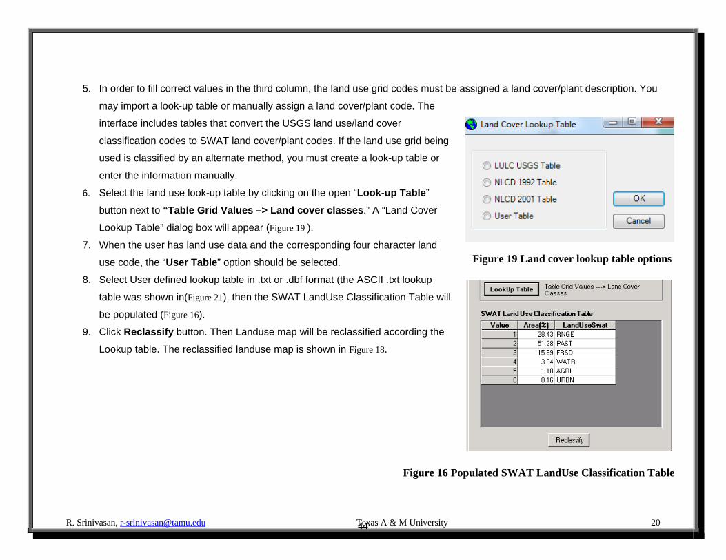
6. Select the land use look-up table by clicking on the open “Look-up Table”
button next to “Table Grid Values –> Land cover classes.” A “Land Cover
Lookup Table” dialog box will appear (Figure 19 ).
7. When the user has land use data and the corresponding four character land
use code, the “User Table” option should be selected.
8. Select User defined lookup table in .txt or .dbf format (the ASCII .txt lookup
table was shown in(Figure 21), then the SWAT LandUse Classification Table will
be populated (Figure 16).
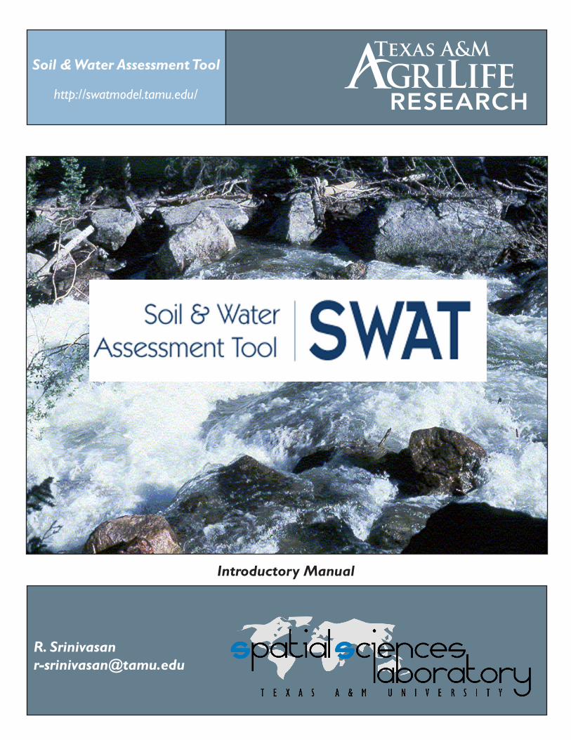
9. Click Reclassify button. Then Landuse map will be reclassified according the
Lookup table. The reclassified landuse map is shown in Figure 18.
Figure 19 Land cover lookup table options
Figure 16 Populated SWAT LandUse Classification Table
44

R. Srinivasan, [email protected] Texas A & M University 21
Accessing “User Table” from the Landuse and soil definition dialog box:
The user defined table has to be created in the format as shown in figure below:
Figure 17 ASCII (.txt) table format of lookup table
Note: 1. To manually create a look-up table, double click on the “LandUseSwat” field next to the first category number in the dialog. A
dialog box will appear listing the two database files from which a SWAT land type may be selected: Land Cover/Plant and Urban. Select the desired database file by clicking on it. Click OK. A dialog box will appear listing the available SWAT land cover codes or the available SWAT urban land type codes. Select the desired code from the list and click ok. Repeat this procedure for all the values in the grid.
2. If you do not find the desired land cover in the database, you will have to add the land cover class to the database too.
45
R. Srinivasan, [email protected] Texas A & M University 23
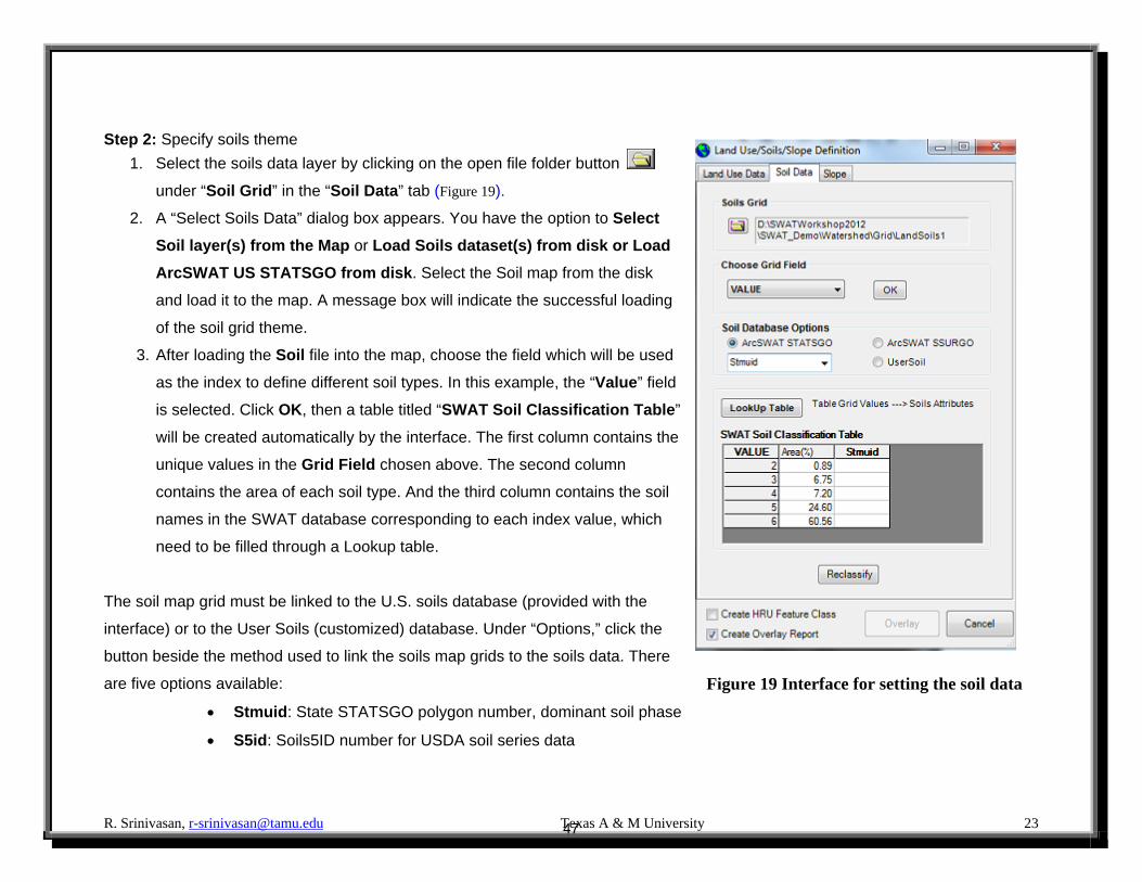
Step 2: Specify soils theme
1. Select the soils data layer by clicking on the open file folder button
under “Soil Grid” in the “Soil Data” tab (Figure 19).
2. A “Select Soils Data” dialog box appears. You have the option to Select
Soil layer(s) from the Map or Load Soils dataset(s) from disk or Load
ArcSWAT US STATSGO from disk. Select the Soil map from the disk
and load it to the map. A message box will indicate the successful loading
of the soil grid theme.
3. After loading the Soil file into the map, choose the field which will be used
as the index to define different soil types. In this example, the “Value” field
is selected. Click OK, then a table titled “SWAT Soil Classification Table”
will be created automatically by the interface. The first column contains the
unique values in the Grid Field chosen above. The second column
contains the area of each soil type. And the third column contains the soil
names in the SWAT database corresponding to each index value, which
need to be filled through a Lookup table.
The soil map grid must be linked to the U.S. soils database (provided with the
interface) or to the User Soils (customized) database. Under “Options,” click the
button beside the method used to link the soils map grids to the soils data. There
are five options available:
Stmuid: State STATSGO polygon number, dominant soil phase
S5id: Soils5ID number for USDA soil series data
Figure 19 Interface for setting the soil data
47

R. Srinivasan, [email protected] Texas A & M University 24
Name: Name of soil in User Soils database
Stmuid + Seqn: State STATSGO polygon number and sequence number of soil phase
Name + Stmuid: State STATSGO polygon number and soil series name
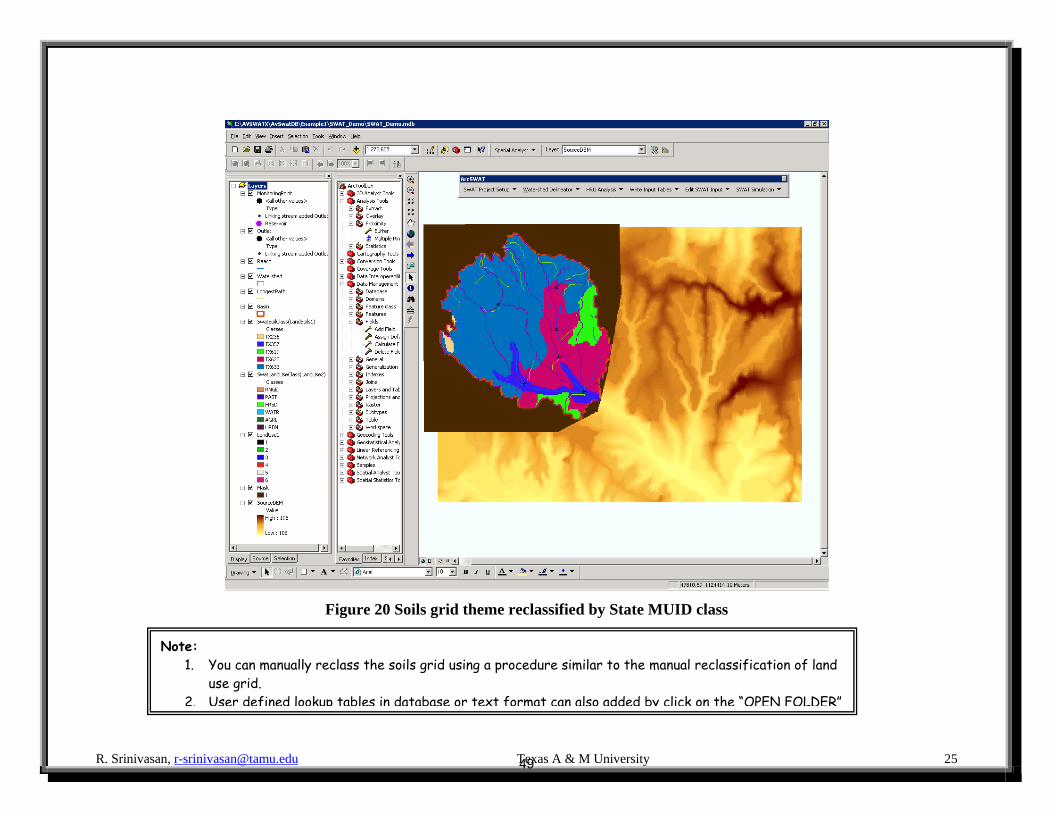
4. Select Stmuid, then load look up values for the soil grid file and click the Reclassify button for soils grid. The reclassified
soils grid (Figure 20) is shown in the map.
Note:
SSURGO soil data can also be used with SWAT. SWAT – SSURGO processing tool is available in http://lcluc.tamu.edu/ssurgo/ .
48
R. Srinivasan, [email protected] Texas A & M University 25
Figure 20 Soils grid theme reclassified by State MUID class
Note: 1. You can manually reclass the soils grid using a procedure similar to the manual reclassification of land
use grid. 2. User defined lookup tables in database or text format can also added by click on the “OPEN FOLDER”
49
R. Srinivasan, [email protected] Texas A & M University 26
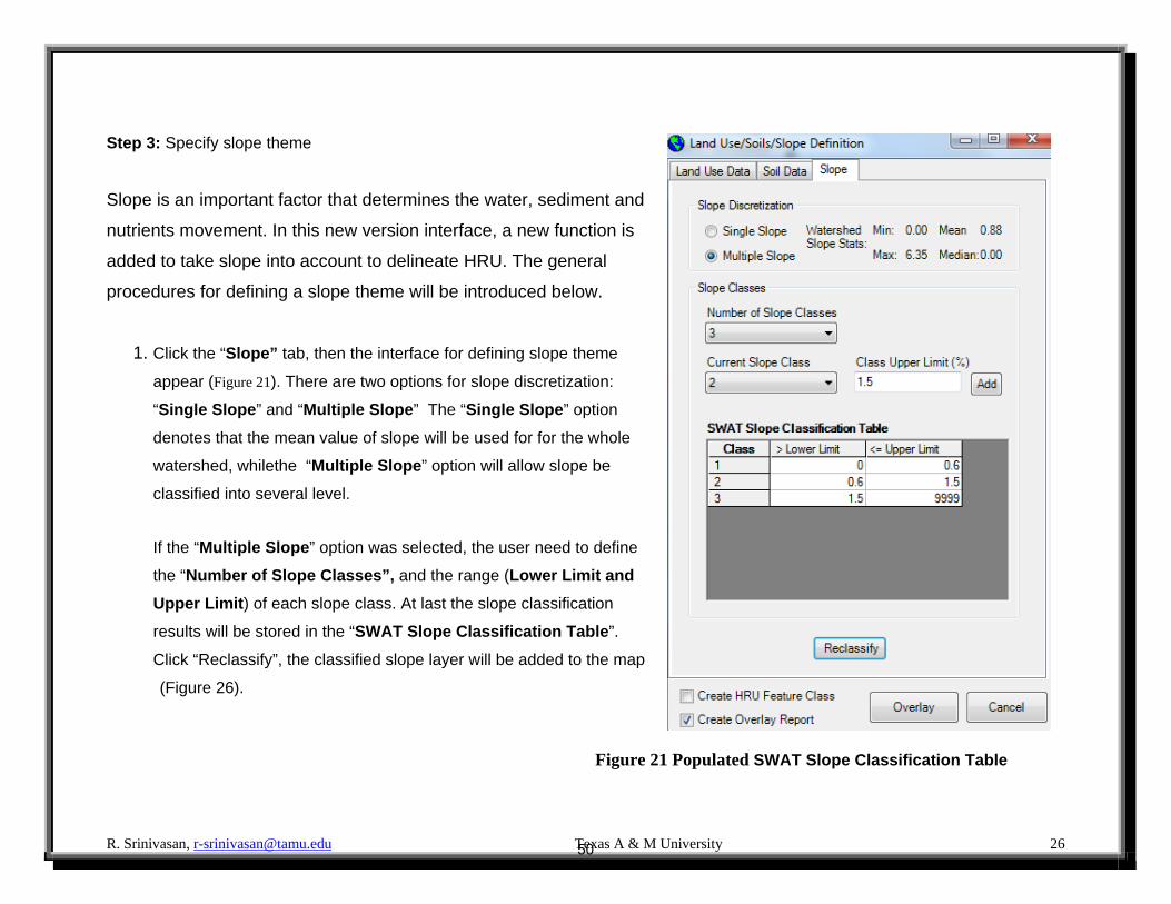
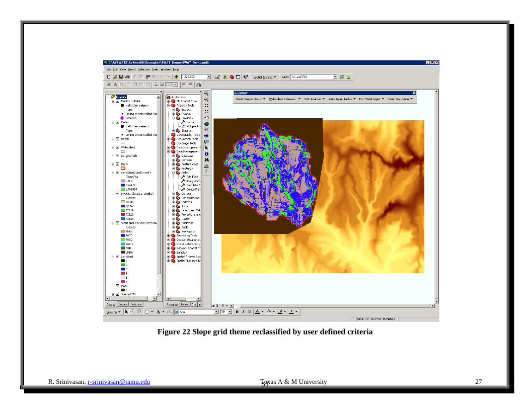
Step 3: Specify slope theme
Slope is an important factor that determines the water, sediment and
nutrients movement. In this new version interface, a new function is
added to take slope into account to delineate HRU. The general
procedures for defining a slope theme will be introduced below.
1. Click the “Slope” tab, then the interface for defining slope theme
appear (Figure 21). There are two options for slope discretization:
“Single Slope” and “Multiple Slope” The “Single Slope” option
denotes that the mean value of slope will be used for for the whole
watershed, whilethe “Multiple Slope” option will allow slope be
classified into several level.
If the “Multiple Slope” option was selected, the user need to define
the “Number of Slope Classes”, and the range (Lower Limit and
Upper Limit) of each slope class. At last the slope classification
results will be stored in the “SWAT Slope Classification Table”.
Click “Reclassify”, the classified slope layer will be added to the map
(Figure 26).
Figure 21 Populated SWAT Slope Classification Table
50
R. Srinivasan, [email protected] Texas A & M University 27
Figure 22 Slope grid theme reclassified by user defined criteria
51
R. Srinivasan, [email protected] Texas A & M University 28
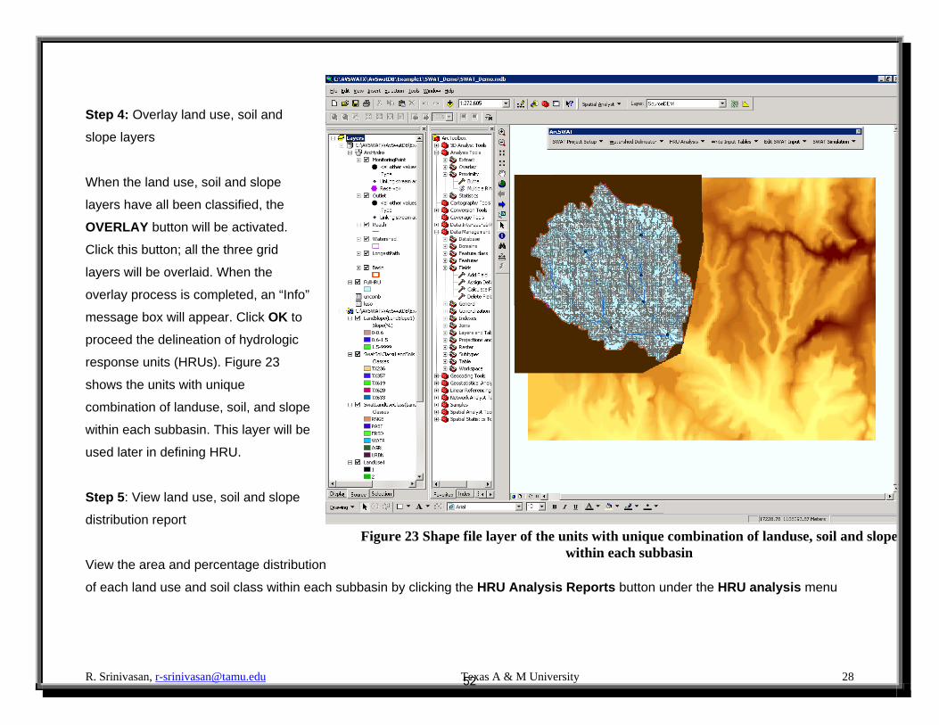
Step 4: Overlay land use, soil and
slope layers
When the land use, soil and slope
layers have all been classified, the
OVERLAY button will be activated.
Click this button; all the three grid
layers will be overlaid. When the
overlay process is completed, an “Info”
message box will appear. Click OK to
proceed the delineation of hydrologic
response units (HRUs). Figure 23
shows the units with unique
combination of landuse, soil, and slope
within each subbasin. This layer will be
used later in defining HRU.
Step 5: View land use, soil and slope
distribution report
View the area and percentage distribution
of each land use and soil class within each subbasin by clicking the HRU Analysis Reports button under the HRU analysis menu
Figure 23 Shape file layer of the units with unique combination of landuse, soil and slope within each subbasin
52
R. Srinivasan, [email protected] 29
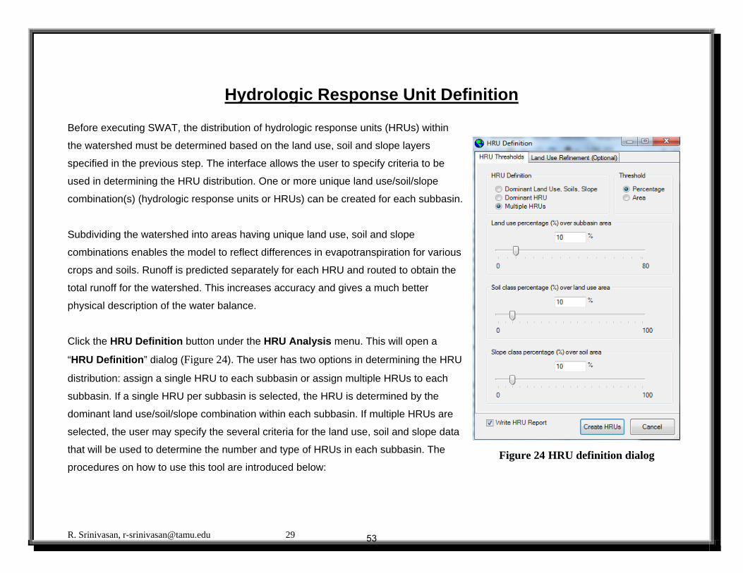
Hydrologic Response Unit Definition
Before executing SWAT, the distribution of hydrologic response units (HRUs) within
the watershed must be determined based on the land use, soil and slope layers
specified in the previous step. The interface allows the user to specify criteria to be
used in determining the HRU distribution. One or more unique land use/soil/slope
combination(s) (hydrologic response units or HRUs) can be created for each subbasin.
Subdividing the watershed into areas having unique land use, soil and slope
combinations enables the model to reflect differences in evapotranspiration for various
crops and soils. Runoff is predicted separately for each HRU and routed to obtain the
total runoff for the watershed. This increases accuracy and gives a much better
physical description of the water balance.
Click the HRU Definition button under the HRU Analysis menu. This will open a
“HRU Definition” dialog (Figure 24). The user has two options in determining the HRU
distribution: assign a single HRU to each subbasin or assign multiple HRUs to each
subbasin. If a single HRU per subbasin is selected, the HRU is determined by the
dominant land use/soil/slope combination within each subbasin. If multiple HRUs are
selected, the user may specify the several criteria for the land use, soil and slope data
that will be used to determine the number and type of HRUs in each subbasin. The
procedures on how to use this tool are introduced below: Figure 24 HRU definition dialog
53
R. Srinivasan, [email protected] Texas A & M University 30
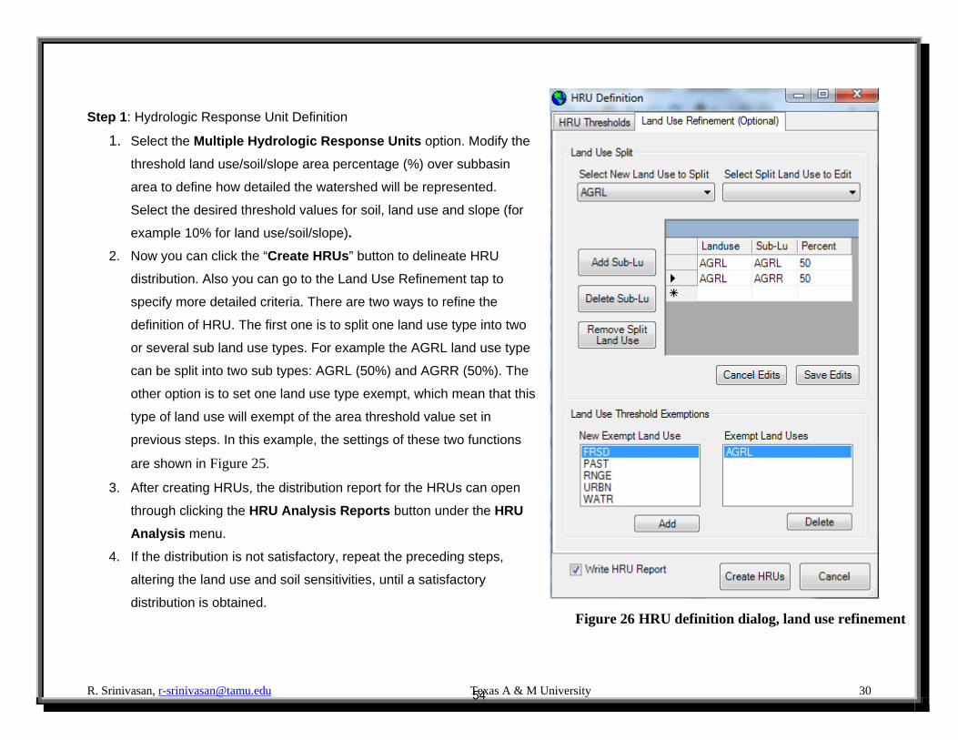
Step 1: Hydrologic Response Unit Definition
1. Select the Multiple Hydrologic Response Units option. Modify the
threshold land use/soil/slope area percentage (%) over subbasin
area to define how detailed the watershed will be represented.
Select the desired threshold values for soil, land use and slope (for
example 10% for land use/soil/slope).
2. Now you can click the “Create HRUs” button to delineate HRU
distribution. Also you can go to the Land Use Refinement tap to
specify more detailed criteria. There are two ways to refine the
definition of HRU. The first one is to split one land use type into two
or several sub land use types. For example the AGRL land use type
can be split into two sub types: AGRL (50%) and AGRR (50%). The
other option is to set one land use type exempt, which mean that this
type of land use will exempt of the area threshold value set in
previous steps. In this example, the settings of these two functions
are shown in Figure 25.
3. After creating HRUs, the distribution report for the HRUs can open
through clicking the HRU Analysis Reports button under the HRU
Analysis menu.
4. If the distribution is not satisfactory, repeat the preceding steps,
altering the land use and soil sensitivities, until a satisfactory
distribution is obtained.
Figure 25 Interface for Land use refinement
Figure 26 HRU definition dialog, land use refinement
54

R. Srinivasan, [email protected] Texas A & M University 31
Note for HRU distribution Selecting Multiple Hydrologic response units option allows us to eliminate minor land uses in each subbasin. For example, if we set the threshold for Landuse (%) over subbasin area to 15% landuses that occupy less that 15% of
subbasin area would be eliminated and the HRU will be created for landuses that occupy greater than 15% of the subbasin area.
The same holds for Soil and slope layer.
55
R. Srinivasan, [email protected] BRC/UT/EPA/BASINS
Soil and Water Assessment Tool (SWAT)
The following are the key procedures necessary for modeling using SWAT.
Create SWAT project
Delineate the designated watershed for modeling
Define land use/soil/slope data grids
Determine the distribution of HRUs based on the land use and soil data
Define rainfall, temperature and other weather data
Write the SWAT input files- requires access to data on soil, weather, land cover, plant growth, fertilizer and pesticide use,
tillage, and urban activities.
Edit the input files – if necessary
Setup and run SWAT – requires information on simulation period, PET estimation method and other options
View SWAT Output
Now we have completed the first three procedures. In this tutorial we will concentrate on preparing the rest of the input data for
SWAT, running the model, and viewing the output from the model.
Note
Spatial analyst is the main tool that will be used in SWAT. Without this, SWAT simply can’t be used. General info about SWAT: All SWAT input and output are in Metric units (MKS)
56
R. Srinivasan, [email protected] Texas A & M University 31
Write Input Tables for SWAT This menu contains functions to build database files that include information needed to generate default input for the SWAT model.
The commands on the menu need to be implemented only once for a project. However, if the user modifies the HRU distribution after
building the input database files, these commands must be reprocessed again.
Step 1: Define Weather data
1. Select the Weather Stations button under the Write Input
Tables menu. A “Weather Data Definition” dialog is opened
(Figure 27). This dialog will allow the user to define the input
data for rainfall, temperature and other weather data. For
weather data, you have the option of simulating the data in
the model or to read from data tables. If no observed weather
data is available, then information can be simulated using a
weather generator based on the data from 1041 weather
stations around the US or combination of WBAN (Weather
Bureau Army Navy) and Cooperative stations for four 30-year
periods stored in a database or custom weather data can be
input through a database table. The weather generator data
must be defined before you can continue to define the other data, like precipitation and temperature.
2. Select the “WGEN_US_FirstOrder” option for Weather Generator Data to add the weather simulation database automatically.
3. Under the “Rainfall data” tab, select the “Raingages” option for rainfall data. Browse to the Work Directory and choose the
file pcpfork.txt and click Add.
Figure 27 Weather Data definition dialog
57
R. Srinivasan, [email protected] Texas A & M University 32
4. Under the “Temperature data” tab, select the “Climate Stations” radio button option for temperature data. Browse to the Work
Directory and choose the file tmpfork.txt and click Add.
5. After selecting the rainfall, temperature and weather generator data, click OK to generate the SWAT weather input data files.
The locations of weather generator, rainfall and temperature gages will be displayed in the map view (Figure 28).
6. A message box will indicate successful generation of SWAT weather input database.
At this point you have the option to generate all the input data files using the WRITE ALL option under the INPUT menu or generate
each input file separately. The input files needed are:
Watershed Configuration file (.fig)
Soil data (.sol)
Weather generator data (.wgn)
General HRU data (.sub)
Soil chemical input (.chm)
Stream water quality input (.swq)
Pond input (.pnd)
Management Input (.mgt)
Main channel data (.rte)
Ground water data (.gw)
Water use data (.wus)
Note In the new version of ArcSWAT (2012), the user can modify the weather data files later without rewriting the input tables. In the previous version (2009) the input files needed to be rewritten after weather data modification and the model parameterizations set to the default values.
58
R. Srinivasan, [email protected] Texas A & M University 33
Figure 28 Location of weather stations
59
R. Srinivasan, [email protected] Texas A & M University 34
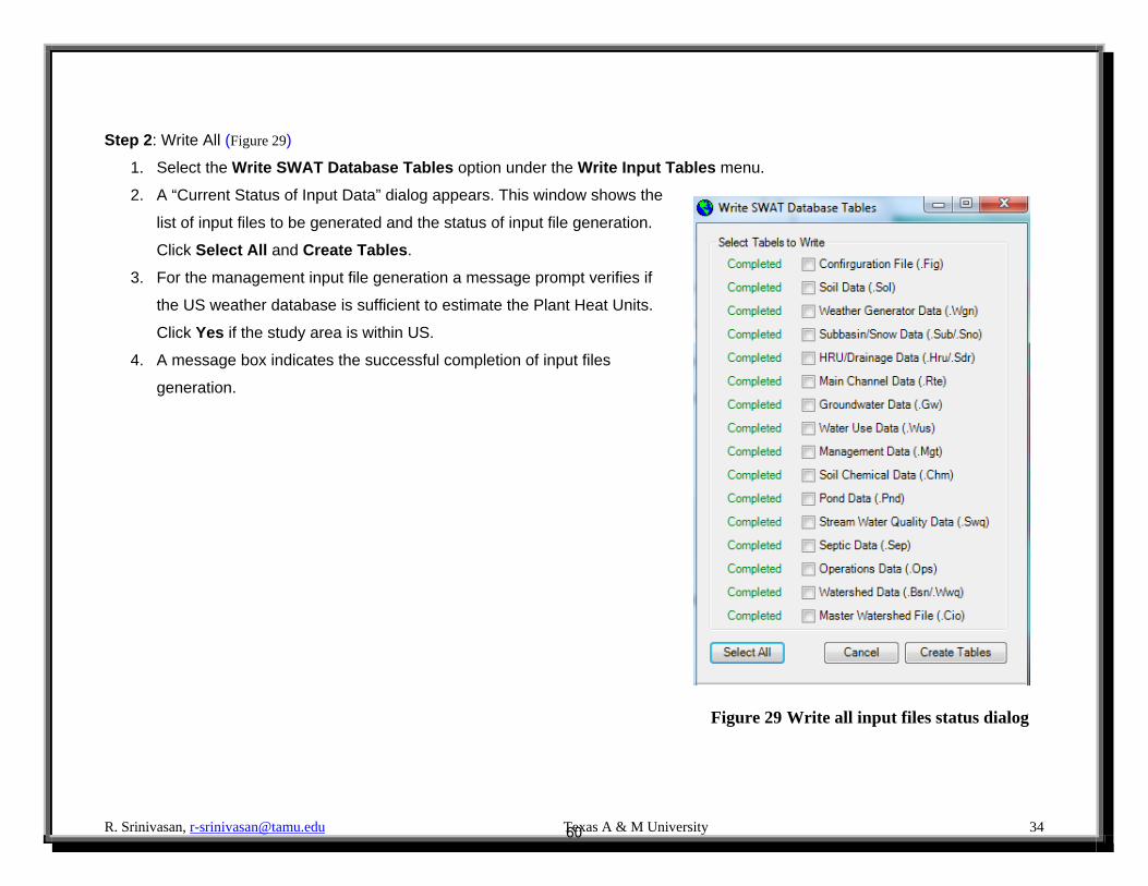
Figure 29 Write all input files status dialog
Step 2: Write All (Figure 29)
1. Select the Write SWAT Database Tables option under the Write Input Tables menu.
2. A “Current Status of Input Data” dialog appears. This window shows the
list of input files to be generated and the status of input file generation.
Click Select All and Create Tables.
3. For the management input file generation a message prompt verifies if
the US weather database is sufficient to estimate the Plant Heat Units.
Click Yes if the study area is within US.
4. A message box indicates the successful completion of input files
generation.
60
R. Srinivasan, [email protected] Texas A & M University 35
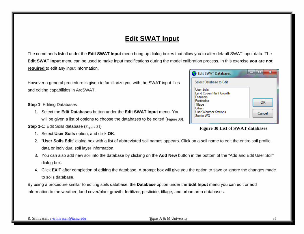
Figure 30 List of SWAT databases
Edit SWAT Input The commands listed under the Edit SWAT Input menu bring up dialog boxes that allow you to alter default SWAT input data. The
Edit SWAT Input menu can be used to make input modifications during the model calibration process. In this exercise you are not
required to edit any input information.
However a general procedure is given to familiarize you with the SWAT input files
and editing capabilities in ArcSWAT.
Step 1: Editing Databases
1. Select the Edit Databases button under the Edit SWAT Input menu. You
will be given a list of options to choose the databases to be edited (Figure 30).
Step 1-1: Edit Soils database (Figure 31)
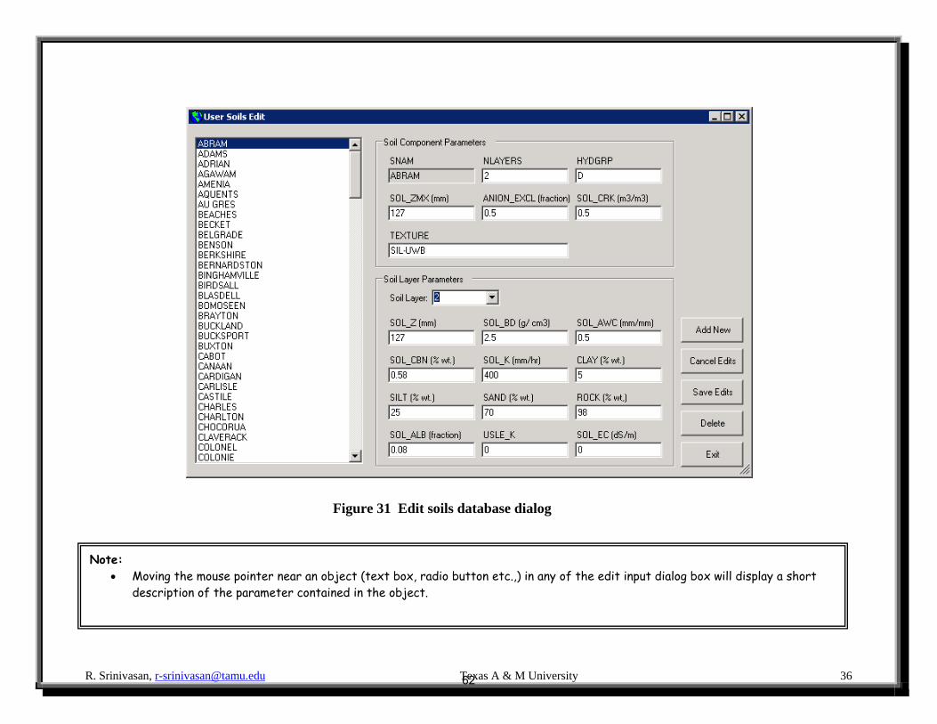
1. Select User Soils option, and click OK.
2. “User Soils Edit” dialog box with a list of abbreviated soil names appears. Click on a soil name to edit the entire soil profile
data or individual soil layer information.
3. You can also add new soil into the database by clicking on the Add New button in the bottom of the “Add and Edit User Soil”
dialog box.
4. Click EXIT after completion of editing the database. A prompt box will give you the option to save or ignore the changes made
to soils database.
By using a procedure similar to editing soils database, the Database option under the Edit Input menu you can edit or add
information to the weather, land cover/plant growth, fertilizer, pesticide, tillage, and urban area databases.
61
R. Srinivasan, [email protected] Texas A & M University 36
Figure 31 Edit soils database dialog
Note: Moving the mouse pointer near an object (text box, radio button etc.,) in any of the edit input dialog box will display a short
description of the parameter contained in the object.
62
R. Srinivasan, [email protected] Texas A & M University 37
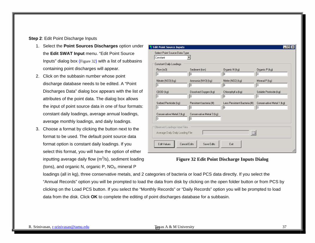
Step 2: Edit Point Discharge Inputs
1. Select the Point Sources Discharges option under
the Edit SWAT Input menu. “Edit Point Source
Inputs” dialog box (Figure 32) with a list of subbasins
containing point discharges will appear.
2. Click on the subbasin number whose point
discharge database needs to be edited. A “Point
Discharges Data” dialog box appears with the list of
attributes of the point data. The dialog box allows
the input of point source data in one of four formats:
constant daily loadings, average annual loadings,
average monthly loadings, and daily loadings.
3. Choose a format by clicking the button next to the
format to be used. The default point source data
format option is constant daily loadings. If you
select this format, you will have the option of either
inputting average daily flow (m3/s), sediment loading
(tons), and organic N, organic P, NO3, mineral P
loadings (all in kg), three conservative metals, and 2 categories of bacteria or load PCS data directly. If you select the
“Annual Records” option you will be prompted to load the data from disk by clicking on the open folder button or from PCS by
clicking on the Load PCS button. If you select the “Monthly Records” or “Daily Records” option you will be prompted to load
data from the disk. Click OK to complete the editing of point discharges database for a subbasin.
Figure 32 Edit Point Discharge Inputs Dialog
63
R. Srinivasan, [email protected] Texas A & M University 38
4. If you wish to edit the point sources in another subbasin, select it from the list in the “Edit Point Source Inputs” dialog box.
Click Exit to complete editing of point discharges database in all subbasins.
Step 3: Edit Inlet Dischargers Input
1. Select the Inlet Discharges option under the Edit
Input menu
2. If there are any inlet dischargers in the project, “Edit
Inlet Input” dialog box with a list of subbasins containing
inlet dischargers will appear (Figure 33).
3. You will be able to modify the inlet input information
using a procedure similar to editing the point
dischargers database
4. The dialog box allows the input of inlet discharge data
in one of four formats: constant daily loadings, average
annual loadings, average monthly loadings, and daily
loadings. Choose a format by clicking the button next to
the format to be used.
5. The default inlet discharge data format option is
constant daily loadings. If you select this format, you will be
prompted to input average daily flow (m3), sediment loading (tons), and organic N, organic P, NO3 and mineral P loadings.
6. If you choose “Annual Records”, “Monthly Records” or “Daily Records” option you will be prompted to load the data from the
disk.
7. Click OK to complete the editing of inlet discharges for a subbasin.
Figure 33 Edit Inlet Discharge Inputs Dialog
64
R. Srinivasan, [email protected] Texas A & M University 39
8. If you wish to edit the inlets in another subbasin, select it from the list in the “Edit Inlet Discharger Input” dialog box. Click Exit
to complete editing of inlet dischargers input in all subbasins
9. Since there are no inlet dischargers defined in this tutorial you will get a message “No Inlet Discharges in the Watershed”
Step 4: Edit Reservoir Input
1. To edit the reservoirs, on the Edit Input menu, select Reservoirs. A dialog box will appear with a list of the subbasins
containing reservoirs.
2. To edit the reservoirs within a subbasin, click on the number of the subbasin in the “Edit Reservoirs Inputs” dialog box.
3. Since there are no reservoirs defined in this project you will get a message “No Reservoirs in the Watershed”.
Step 5: Edit Subbasins Data
1. To edit the subbasin input files, select the Subbasins Data
option under the Edit Input menu. “Edit Subbasin Inputs”
dialog box will appear (Figure 37).
This dialog box contains the list of subbasins, land uses, soil
types and slope levels within each subbasin and the input
files corresponding to each subbasin/land use/soil/slope
combination. To select an input file, select the subbasin, land
use, soil type and slope that you would like to edit. When you
select a subbasin, the combo box of land uses, soil types, and
slope levels will be activated in sequence. Specify the subbasin/land use/soil combination of interest by selecting each
category in the combo box.
Figure 34 Edit Subbasin Inputs main dialog
65
R. Srinivasan, [email protected] Texas A & M University 40
2. To edit the soil physical data, click on the .sol extension, and select the subbasin number, landuse type, soil type and slope
level. Then the OK button is activated. Click OK; a new dialog box will appear (Figure 35). Click the Edit Values button; all the
boxes are activated and the user can revise the default values.
3. The interface allows the user to save the revision of current .sol file to other .sol files. Three options are available: 1) extend
edits to current HRU, which is the default setting, 2) extend edits to all HRUs, or 3) extend edits to selected HRUs. For the
third option, the user needs to specify the subbasin number, landuse type, soil type and slope levels for the HRUs that the
user wants to apply current .sol file parameters.
Figure 35 Edit soil input file dialog
66
R. Srinivasan, [email protected] Texas A & M University 41
4. To edit the weather generator data click on the .wgn extension. For the .wgn file you only need to select the subbasin
number, and then the OK button will be activated. Click OK; a new dialog box (Figure 36) will appear which will allow you to
modify the data in .wgn file. Similar to .sol file, the interface also allow the user to extend the current edits to other subbasins.
The user can select to 1) extend edits to current Subbasin, which is the default setting, 2) extend edits to all Subbasins, or 3)
extend edits to selected Subbasins.
Figure 36 Edit weather generator input file main dialog
67
R. Srinivasan, [email protected] Texas A & M University 42
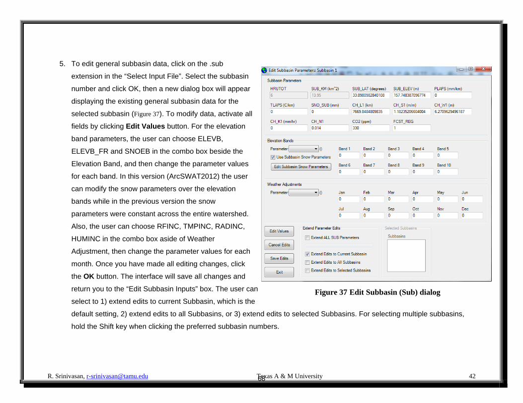
5. To edit general subbasin data, click on the .sub
extension in the “Select Input File”. Select the subbasin
number and click OK, then a new dialog box will appear
displaying the existing general subbasin data for the
selected subbasin (Figure 37). To modify data, activate all
fields by clicking Edit Values button. For the elevation
band parameters, the user can choose ELEVB,
ELEVB_FR and SNOEB in the combo box beside the
Elevation Band, and then change the parameter values
for each band. In this version (ArcSWAT2012) the user
can modify the snow parameters over the elevation
bands while in the previous version the snow
parameters were constant across the entire watershed.
Also, the user can choose RFINC, TMPINC, RADINC,
HUMINC in the combo box aside of Weather
Adjustment, then change the parameter values for each
month. Once you have made all editing changes, click
the OK button. The interface will save all changes and
return you to the “Edit Subbasin Inputs” box. The user can
select to 1) extend edits to current Subbasin, which is the
default setting, 2) extend edits to all Subbasins, or 3) extend edits to selected Subbasins. For selecting multiple subbasins,
hold the Shift key when clicking the preferred subbasin numbers.
Figure 37 Edit Subbasin (Sub) dialog
68
R. Srinivasan, [email protected] Texas A & M University 43
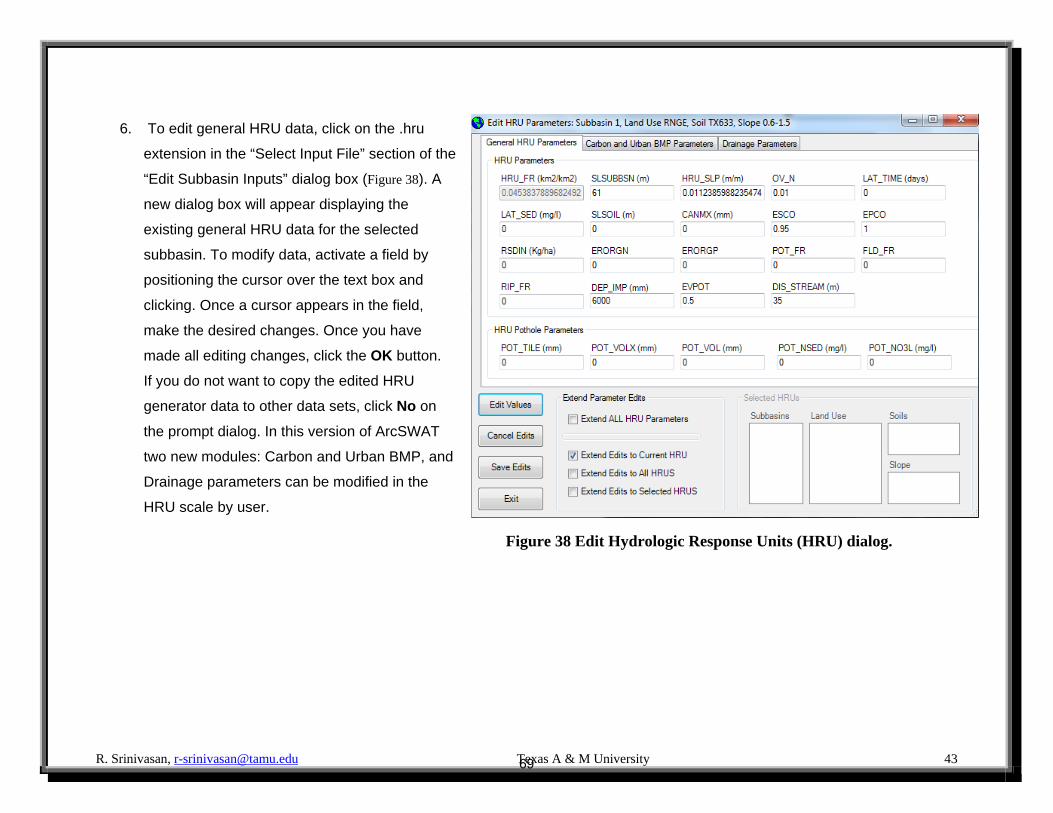
6. To edit general HRU data, click on the .hru
extension in the “Select Input File” section of the
“Edit Subbasin Inputs” dialog box (Figure 38). A
new dialog box will appear displaying the
existing general HRU data for the selected
subbasin. To modify data, activate a field by
positioning the cursor over the text box and
clicking. Once a cursor appears in the field,
make the desired changes. Once you have
made all editing changes, click the OK button.
If you do not want to copy the edited HRU
generator data to other data sets, click No on
the prompt dialog. In this version of ArcSWAT
two new modules: Carbon and Urban BMP, and
Drainage parameters can be modified in the
HRU scale by user.
Figure 38 Edit Hydrologic Response Units (HRU) dialog.
69
R. Srinivasan, [email protected] Texas A & M University 44
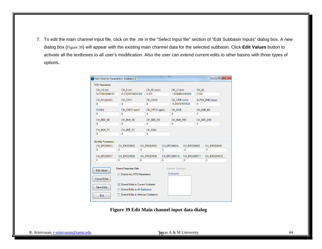
7. To edit the main channel input file, click on the .rte in the “Select Input file” section of “Edit Subbasin Inputs” dialog box. A new
dialog box (Figure 39) will appear with the existing main channel data for the selected subbasin. Click Edit Values button to
activate all the textboxes to all user’s modification. Also the user can extend current edits to other basins with three types of
options.
Figure 39 Edit Main channel input data dialog
70
R. Srinivasan, [email protected] Texas A & M University 45
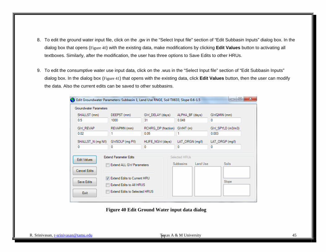
8. To edit the ground water input file, click on the .gw in the “Select Input file” section of “Edit Subbasin Inputs” dialog box. In the
dialog box that opens (Figure 40) with the existing data, make modifications by clicking Edit Values button to activating all
textboxes. Similarly, after the modification, the user has three options to Save Edits to other HRUs.
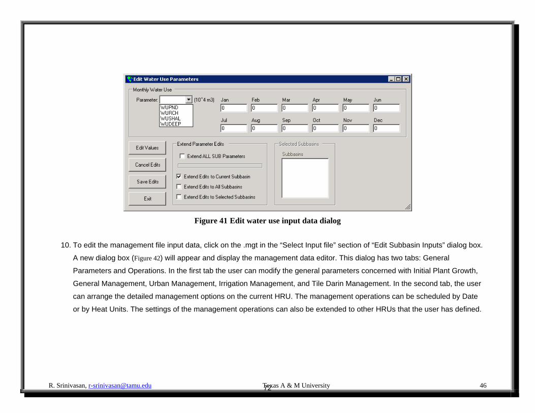
9. To edit the consumptive water use input data, click on the .wus in the “Select Input file” section of “Edit Subbasin Inputs”
dialog box. In the dialog box (Figure 41) that opens with the existing data, click Edit Values button, then the user can modify
the data. Also the current edits can be saved to other subbasins.
Figure 40 Edit Ground Water input data dialog
71
R. Srinivasan, [email protected] Texas A & M University 46
Figure 41 Edit water use input data dialog
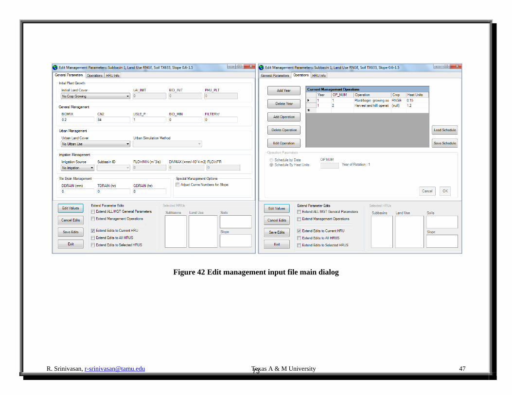
10. To edit the management file input data, click on the .mgt in the “Select Input file” section of “Edit Subbasin Inputs” dialog box.
A new dialog box (Figure 42) will appear and display the management data editor. This dialog has two tabs: General
Parameters and Operations. In the first tab the user can modify the general parameters concerned with Initial Plant Growth,
General Management, Urban Management, Irrigation Management, and Tile Darin Management. In the second tab, the user
can arrange the detailed management options on the current HRU. The management operations can be scheduled by Date
or by Heat Units. The settings of the management operations can also be extended to other HRUs that the user has defined.
72
R. Srinivasan, [email protected] Texas A & M University 47
Figure 42 Edit management input file main dialog
73
R. Srinivasan, [email protected] Texas A & M University 48
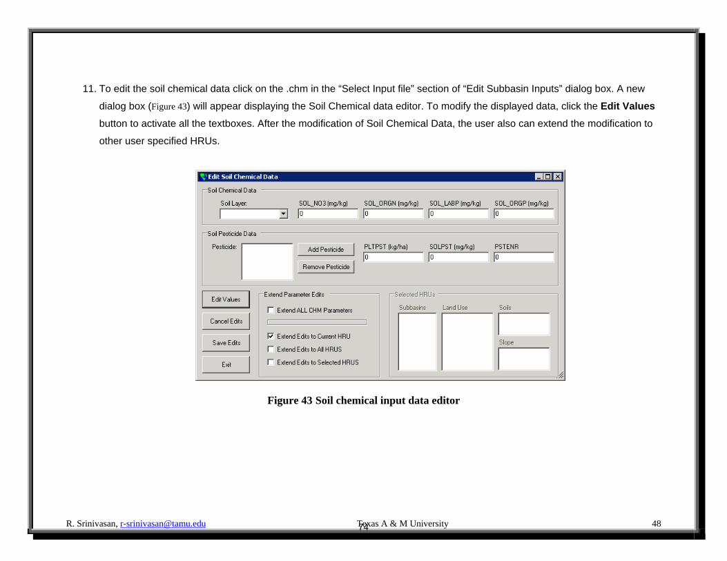
11. To edit the soil chemical data click on the .chm in the “Select Input file” section of “Edit Subbasin Inputs” dialog box. A new
dialog box (Figure 43) will appear displaying the Soil Chemical data editor. To modify the displayed data, click the Edit Values
button to activate all the textboxes. After the modification of Soil Chemical Data, the user also can extend the modification to
other user specified HRUs.
Figure 43 Soil chemical input data editor
74
R. Srinivasan, [email protected] Texas A & M University 49
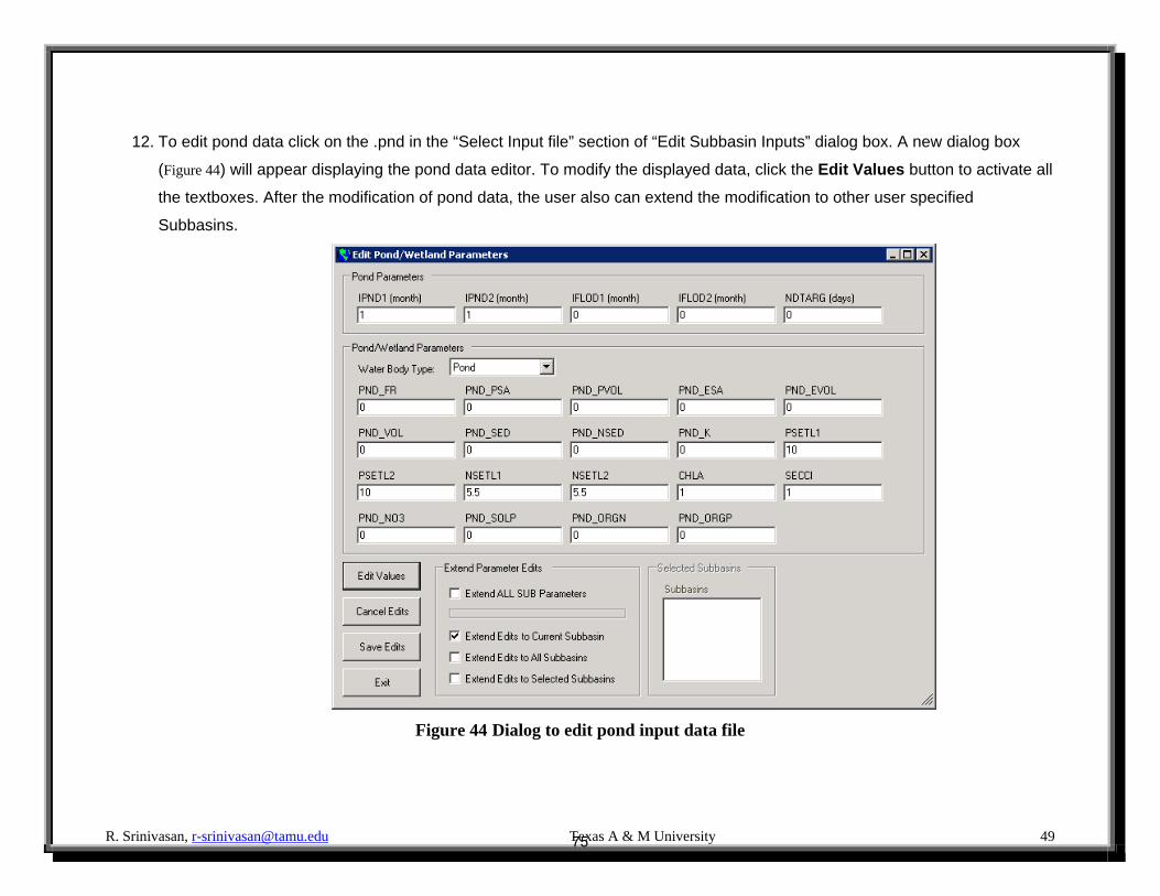
12. To edit pond data click on the .pnd in the “Select Input file” section of “Edit Subbasin Inputs” dialog box. A new dialog box
(Figure 44) will appear displaying the pond data editor. To modify the displayed data, click the Edit Values button to activate all
the textboxes. After the modification of pond data, the user also can extend the modification to other user specified
Subbasins.
Figure 44 Dialog to edit pond input data file
75
R. Srinivasan, [email protected] Texas A & M University 50
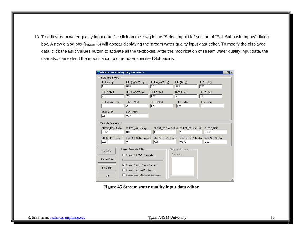
13. To edit stream water quality input data file click on the .swq in the “Select Input file” section of “Edit Subbasin Inputs” dialog
box. A new dialog box (Figure 45) will appear displaying the stream water quality input data editor. To modify the displayed
data, click the Edit Values button to activate all the textboxes. After the modification of stream water quality input data, the
user also can extend the modification to other user specified Subbasins.
Figure 45 Stream water quality input data editor
76
R. Srinivasan, [email protected] Texas A & M University 51
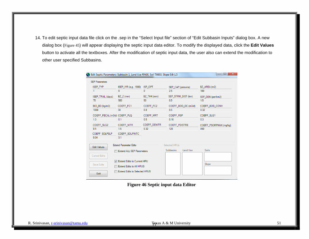
14. To edit septic input data file click on the .sep in the “Select Input file” section of “Edit Subbasin Inputs” dialog box. A new
dialog box (Figure 45) will appear displaying the septic input data editor. To modify the displayed data, click the Edit Values
button to activate all the textboxes. After the modification of septic input data, the user also can extend the modification to
other user specified Subbasins.
Figure 46 Septic input data Editor
77
R. Srinivasan, [email protected] Texas A & M University 52
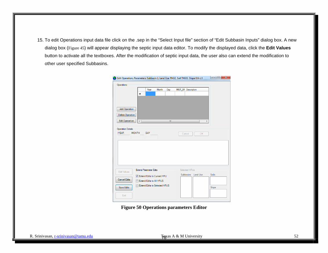
15. To edit Operations input data file click on the .sep in the “Select Input file” section of “Edit Subbasin Inputs” dialog box. A new
dialog box (Figure 45) will appear displaying the septic input data editor. To modify the displayed data, click the Edit Values
button to activate all the textboxes. After the modification of septic input data, the user also can extend the modification to
other user specified Subbasins.
Figure 50 Operations parameters Editor
78
R. Srinivasan, [email protected] Texas A & M University 53
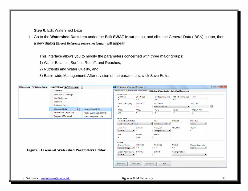
Step 6. Edit Watershed Data
1. Go to the Watershed Data item under the Edit SWAT Input menu, and click the General Data (.BSN) button, then
a new dialog (Error! Reference source not found.) will appear.
This interface allows you to modify the parameters concerned with three major groups:
1) Water Balance, Surface Runoff, and Reaches,
2) Nutrients and Water Quality, and
3) Basin-wide Management. After revision of the parameters, click Save Edits.
Figure 51 General Watershed Parameters Editor
79
R. Srinivasan, [email protected] Texas A & M University 54
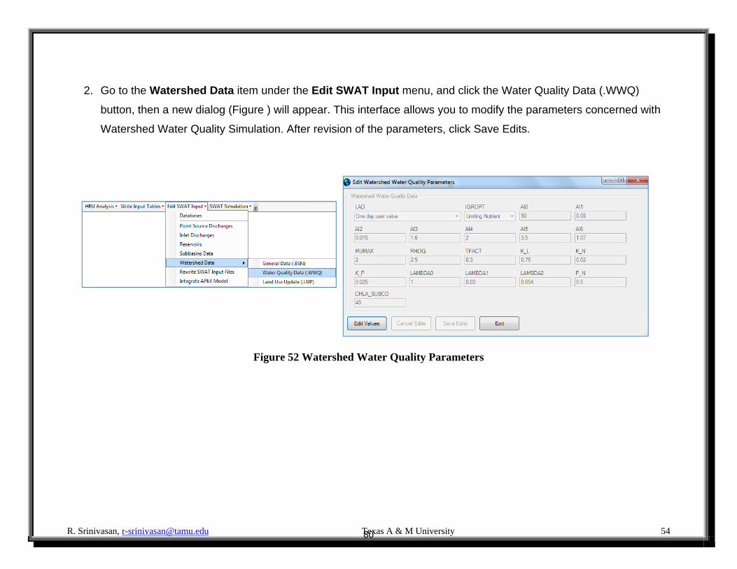
2. Go to the Watershed Data item under the Edit SWAT Input menu, and click the Water Quality Data (.WWQ)
button, then a new dialog (Figure ) will appear. This interface allows you to modify the parameters concerned with
Watershed Water Quality Simulation. After revision of the parameters, click Save Edits.
Figure 52 Watershed Water Quality Parameters
80
R. Srinivasan, [email protected] Texas A & M University 55
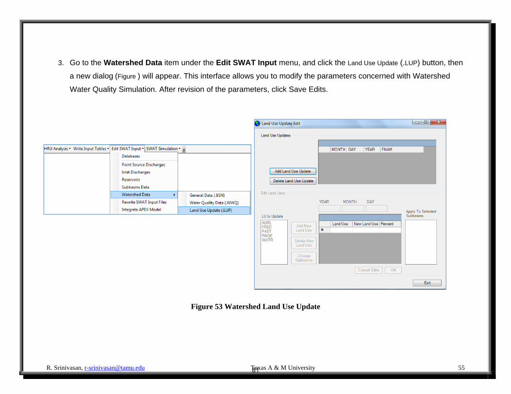
3. Go to the Watershed Data item under the Edit SWAT Input menu, and click the Land Use Update (.LUP) button, then
a new dialog (Figure ) will appear. This interface allows you to modify the parameters concerned with Watershed
Water Quality Simulation. After revision of the parameters, click Save Edits.
Figure 53 Watershed Land Use Update
81
R. Srinivasan, [email protected] Texas A & M University 56
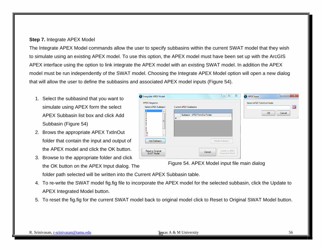
Step 7. Integrate APEX Model
The Integrate APEX Model commands allow the user to specify subbasins within the current SWAT model that they wish
to simulate using an existing APEX model. To use this option, the APEX model must have been set up with the ArcGIS
APEX interface using the option to link integrate the APEX model with an existing SWAT model. In addition the APEX
model must be run independently of the SWAT model. Choosing the Integrate APEX Model option will open a new dialog
that will allow the user to define the subbasins and associated APEX model inputs (Figure 54).
1. Select the subbasind that you want to
simulate using APEX form the select
APEX Subbasin list box and click Add
Subbasin (Figure 54)
2. Brows the appropriate APEX TxtInOut
folder that contain the input and output of
the APEX model and click the OK button.
3. Browse to the appropriate folder and click
the OK button on the APEX Input dialog. The
folder path selected will be written into the Current APEX Subbasin table.
4. To re-write the SWAT model fig.fig file to incorporate the APEX model for the selected subbasin, click the Update to
APEX Integrated Model button.
5. To reset the fig.fig for the current SWAT model back to original model click to Reset to Original SWAT Model button.
Figure 54. APEX Model input file main dialog
82
R. Srinivasan, [email protected] Texas A & M University 57
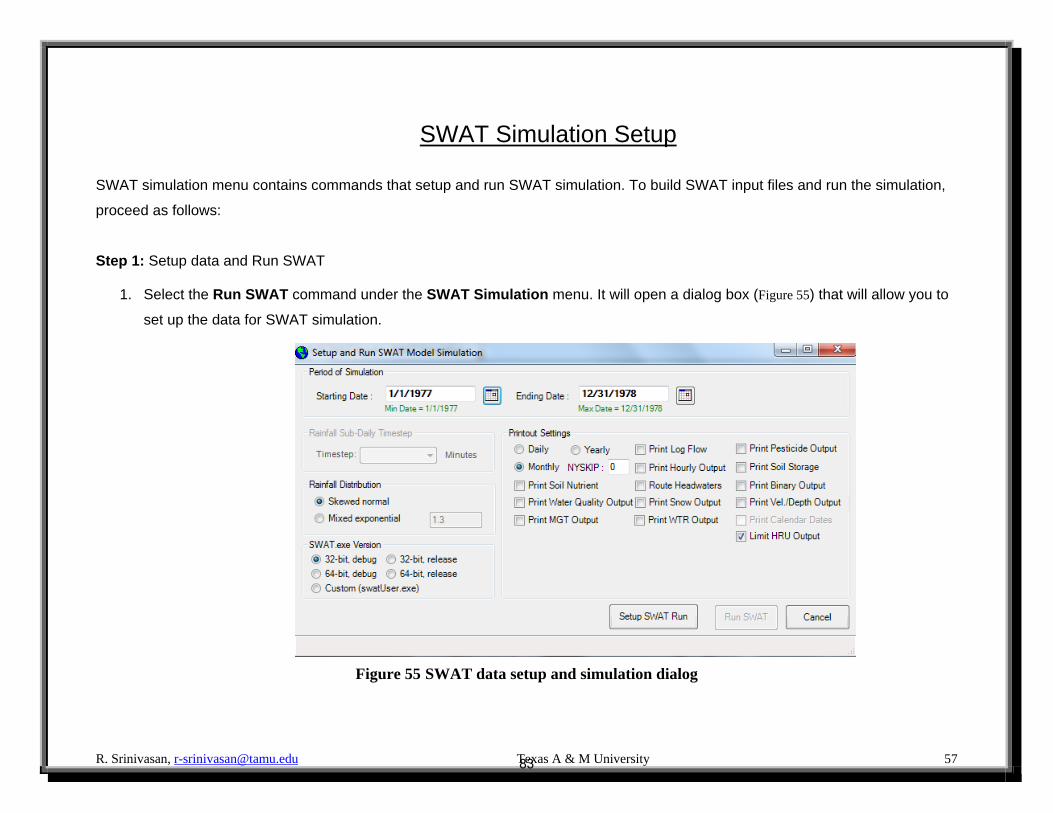
SWAT Simulation Setup
SWAT simulation menu contains commands that setup and run SWAT simulation. To build SWAT input files and run the simulation,
proceed as follows:
Step 1: Setup data and Run SWAT
1. Select the Run SWAT command under the SWAT Simulation menu. It will open a dialog box (Figure 55) that will allow you to
set up the data for SWAT simulation.
Figure 55 SWAT data setup and simulation dialog
83
R. Srinivasan, [email protected] Texas A & M University 58
Figure 56. SWAT Simulation menu
2. Select the 1/1/1977 for the “Starting date” and 12/31/1978 for the “Ending date” option. If you are using simulated rainfall
and temperature data, both these fields will be blank and you have to input the information manually.
3. Choose “monthly” option for Printout Frequency
4. Keep the rest at the default selections.
5. After all the parameters have been set, click the Setup SWAT Run button in the “Run SWAT” dialog box (Figure ) to build the
SWAT CIO, COD, PCP.PCP and TMP.TMP input files. Once all input files are setup, the Run SWAT button is activated in the
bottom right of the Run SWAT dialog.
6. Click the button labeled Run SWAT. This will run the SWAT executable file. A message box will indicate the successful
completion of SWAT run.
Step 2: Read SWAT Output
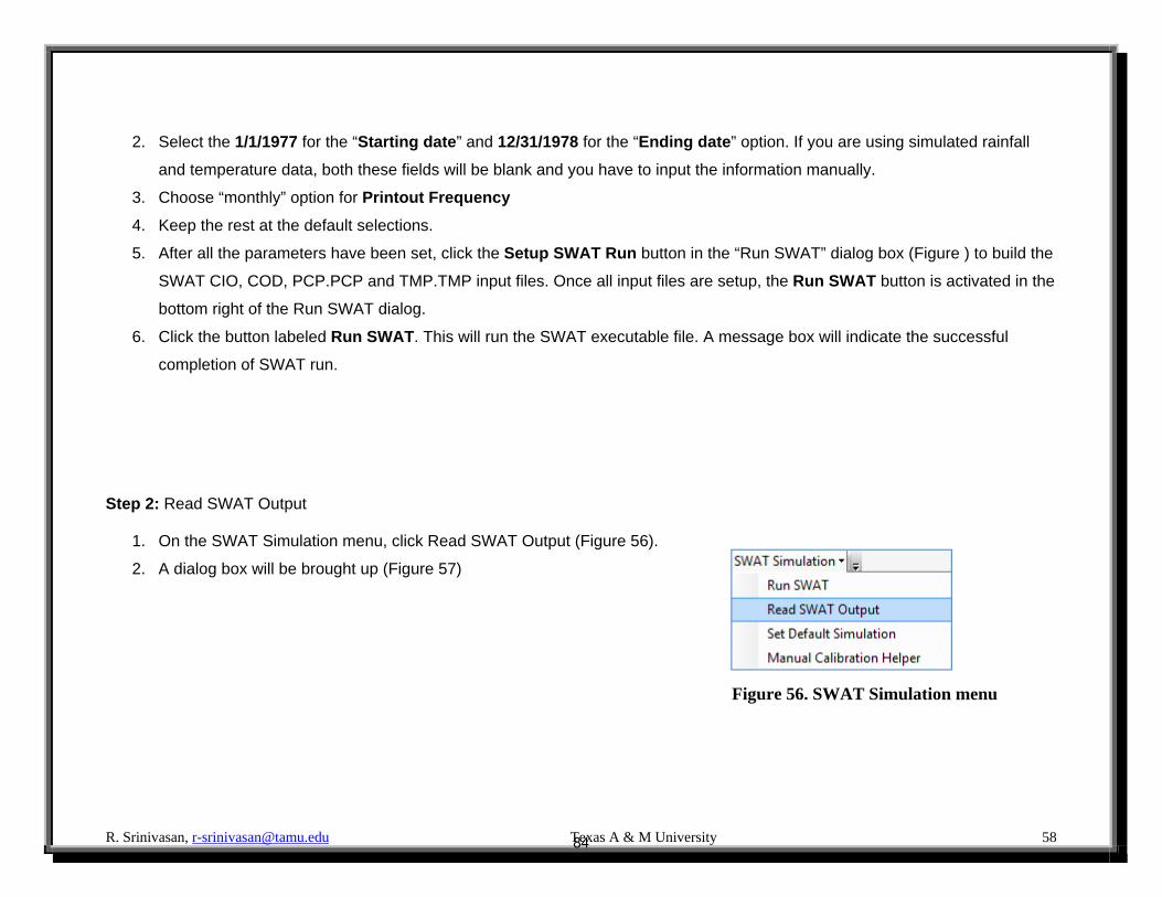
1. On the SWAT Simulation menu, click Read SWAT Output (Figure 56).
2. A dialog box will be brought up (Figure 57)
84
R. Srinivasan, [email protected] Texas A & M University 59
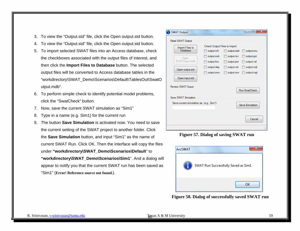
3. To view the “Output.std” file, click the Open output.std button.
4. To view the “Output.std” file, click the Open output.std button.
5. To import selected SWAT files into an Access database, check
the checkboxes associated with the output files of interest, and
then click the Import Files to Database button. The selected
output files will be converted to Access database tables in the
“workdirectory\SWAT_Demo\Scenarios\Default\TablesOut\SwatO
utput.mdb”.
6. To perform simple check to identify potential model problems,
click the “SwatCheck” button.
7. Now, save the current SWAT simulation as “Sim1”
8. Type in a name (e.g. Sim1) for the current run
9. The button Save Simulation is activated now. You need to save
the current setting of the SWAT project to another folder. Click
the Save Simulation button, and input “Sim1” as the name of
current SWAT Run. Click OK. Then the interface will copy the files
under “workdirectory\SWAT_Demo\Scenarios\Default” to
“workdirectory\SWAT_Demo\Scenarios\Sim1”. And a dialog will
appear to notify you that the current SWAT run has been saved as
“Sim1” (Error! Reference source not found.).
Figure 57. Dialog of saving SWAT run
Figure 58. Dialog of successfully saved SWAT run
85
R. Srinivasan, [email protected] Texas A & M University 60
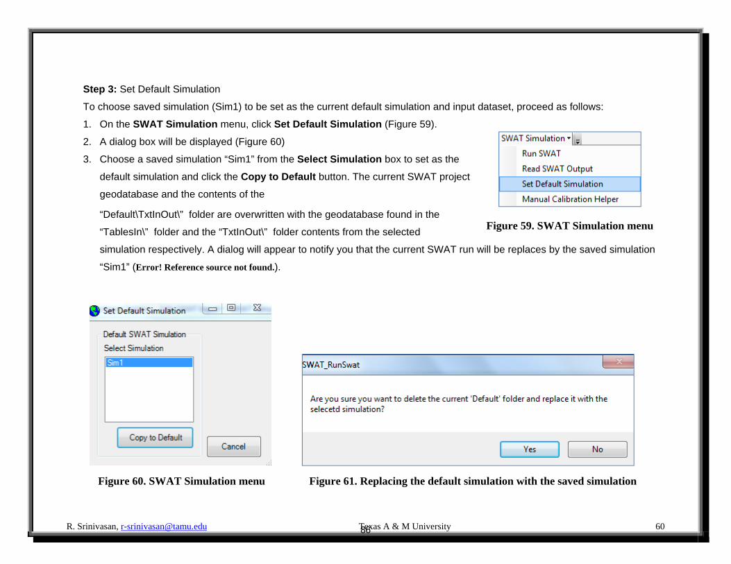
Step 3: Set Default Simulation
To choose saved simulation (Sim1) to be set as the current default simulation and input dataset, proceed as follows:
1. On the SWAT Simulation menu, click Set Default Simulation (Figure 59).
2. A dialog box will be displayed (Figure 60)
3. Choose a saved simulation “Sim1” from the Select Simulation box to set as the
default simulation and click the Copy to Default button. The current SWAT project
geodatabase and the contents of the
“Default\TxtInOut\” folder are overwritten with the geodatabase found in the
“TablesIn\” folder and the “TxtInOut\” folder contents from the selected
simulation respectively. A dialog will appear to notify you that the current SWAT run will be replaces by the saved simulation
“Sim1” (Error! Reference source not found.).
Figure 59. SWAT Simulation menu
Figure 60. SWAT Simulation menu Figure 61. Replacing the default simulation with the saved simulation
86
R. Srinivasan, [email protected] Texas A & M University 61
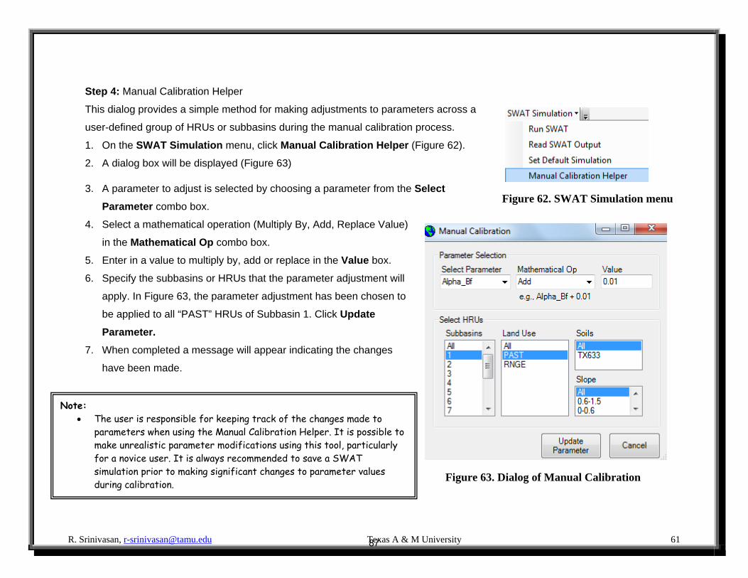
Step 4: Manual Calibration Helper
This dialog provides a simple method for making adjustments to parameters across a
user-defined group of HRUs or subbasins during the manual calibration process.
1. On the SWAT Simulation menu, click Manual Calibration Helper (Figure 62).
2. A dialog box will be displayed (Figure 63)
3. A parameter to adjust is selected by choosing a parameter from the Select
Parameter combo box.
4. Select a mathematical operation (Multiply By, Add, Replace Value)
in the Mathematical Op combo box.
5. Enter in a value to multiply by, add or replace in the Value box.
6. Specify the subbasins or HRUs that the parameter adjustment will
apply. In Figure 63, the parameter adjustment has been chosen to
be applied to all “PAST” HRUs of Subbasin 1. Click Update
Parameter.
7. When completed a message will appear indicating the changes
have been made.
Figure 62. SWAT Simulation menu
Figure 63. Dialog of Manual Calibration
Note: The user is responsible for keeping track of the changes made to
parameters when using the Manual Calibration Helper. It is possible to make unrealistic parameter modifications using this tool, particularly for a novice user. It is always recommended to save a SWAT simulation prior to making significant changes to parameter values during calibration.
87

R. Srinivasan, [email protected] Texas A & M University 62
Appendix: Installing ArcSWAT System Requirements
The SWAT2012/ArcSWAT 2012.10_0.1 Beta8 Interface requires:
Hardware:
Personal computer using a Pentium IV processor or higher, which runs at 2 gigahertz or faster 1 GB RAM minimum 500 megabytes free memory on the hard drive for minimal installation and up to 1.25 gigabyte for a full installation
(including sample datasets and US STATSGO data)
Software (ArcSWAT 2012.10_0.1 for ArcGIS 10 version):
Microsoft Windows XP, or Windows 2000 operating system with most recent kernel patch* ArcGIS-ArcView 10 with service pack 5 (Build 4400) ArcGIS Spatial Analyst 10 extension ArcGIS Developer Kit (usually found in C:\Program Files\ArcGIS\DeveloperKit\) ArcGIS DotNet support (usually found in C:\Program Files\ArcGIS\DotNet\) Microsoft .Net Framework 2.0 Adobe Acrobat Reader version 7 or higher
Microsoft constantly updates the different versions of windows. This interface was developed with the latest version of Windows
and may not run with earlier versions. Patches are available from Microsoft.
88

R. Srinivasan, [email protected] Texas A & M University 63
Using the ArcSWAT Setup Wizard:
After downloading the ArcSWAT program, open the ArcSWAT_Install_1.0.0 folder. Click the icon to begin
installation. Follow the installation wizard instructions.
Select the appropriate folder location for the program, preferably the computer’s main hard drive. Click the Disk Cost button to ensure enough disk space
for installation.
Indicate if program access will be for everyone who uses the computer or just the installer.
89
R. Srinivasan, [email protected] Texas A & M University 64
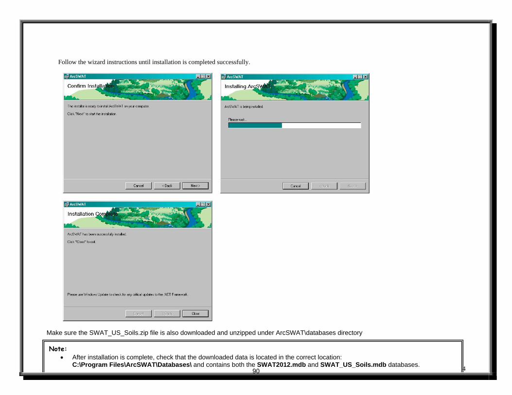
Follow the wizard instructions until installation is completed successfully.
Make sure the SWAT_US_Soils.zip file is also downloaded and unzipped under ArcSWAT\databases directory
Note: After installation is complete, check that the downloaded data is located in the correct location:
C:\Program Files\ArcSWAT\Databases\ and contains both the SWAT2012.mdb and SWAT_US_Soils.mdb databases. 90
R. Srinivasan, [email protected] Texas A & M University 65
Additional information on ArcSWAT installation: What are the build numbers for all the recent releases of ArcGIS?
http://support.esri.com/index.cfm?fa=knowledgebase.techArticles.articleShow&d=30104
You need ArcGIS Desktop 10 Service Pack 5:
http://support.esri.com/en/downloads/patches-ServicePacks/view/productid/159/metaid/1892
How to install ArcGIS 10 with .NET support?
1. Insert the ArcView or ArcGIS Desktop installation disk.
2. Select Install ArcGIS Desktop.
3. Select Modify.
4. Expand Applications; verify that '.NET Support' is installed. If you see a red X, click on the X and select 'Entire feature will be installed' and then follow the rest of the wizard.
91

92
SWAT cAliBrATion TechniqueS
Section 3
93

94
SWAT Calibration Techniques
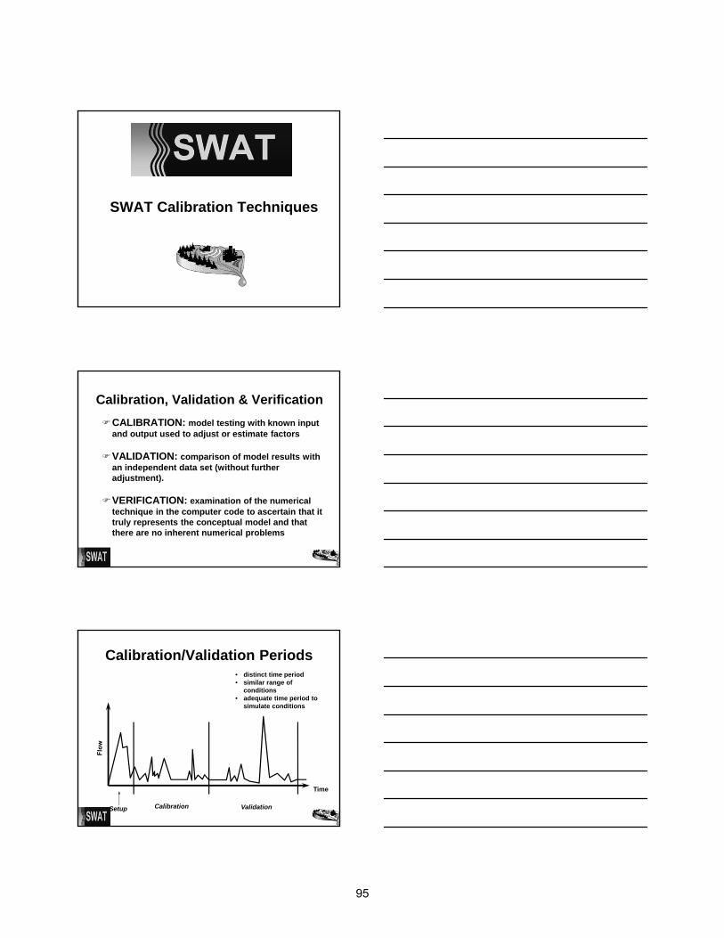
Calibration, Validation & Verification
CALIBRATION: model testing with known input and output used to adjust or estimate factors
VALIDATION: comparison of model results with an independent data set (without further adjustment).
VERIFICATION: examination of the numerical technique in the computer code to ascertain that it truly represents the conceptual model and that there are no inherent numerical problems
Calibration/Validation Periods
Time
Calibration ValidationSetup
• distinct time period• similar range of
conditions• adequate time period to
simulate conditions
95

Model Configuration Land use categories
– land use types in watershed, existing and future land uses, management techniques employed, management questions
Subwatersheds– location, physical characteristics/soils, gaging station
locations, topographic features, management questions.
Reaches– topographic features, stream morphology, cross-section
data available
Calibration Issues:• individual land use parameter determination• location of gaging station data• location of water quality monitoring information• available information on stream systems
Model ConfigurationCalibration Points Example
LEGEND
Calibration/ValidationProcedures
Hydrology - first and foremost Sediment - next Water quality - last (nitrogen, phosphorus,
pesticides, DO, bacteria)
Check list for model testing water balance - is it all accounted for? time series annual total - stream flow & base flow monthly/seasonal total frequency duration curve sediment and nutrients balance
96

Calibration Time Step
Calibration sequence– annual water balance
– seasonal variability
– storm variability time series plot
frequency duration curve
– baseflow
– overall time series
Calibration/Validation Statistics
– Mean and standard deviation of the simulated and measured data
– Slope, intercept and regression coefficient/coefficient of determination
– Nash-Suttcliffe Efficiency
Calibration/ValidationCommon Problems
too little data - too short a monitoring period
small range of conditions– only small storms– only storms during the spring...
prediction of future conditions which are outside the model conditions
calibration/validation does not adequately test separate pieces of model– accuracy of each land use category prediction
calibration adjustments destroy physical representation of system by model
adjustment of the wrong parameters
97
Calibration/ValidationSuggested References
Neitsch, S. L., J. G. Arnold, J. R. Kiniry and J. R. Willams. 2001. Soil and WaterAssessment Tool – Manual, USDA-ARS Publications. pp: 341-354.http://www.brc.tamus.edu/swat/manual.
Santhi, C., J. G. Arnold, J. R. Williams, W. A. Dugas, R. Srinivasan and L. M. Hauck.2001. Validation of the SWAT Model on a Large River Basin with Point and NonpointSources. J. American Water Resources Association 37(5): 1169-1188.
Srinivasan, R., T. S. Ramanarayanan, J. G. Arnold and S. T. Bednarz. 1997. Large areahydrologic modeling and assessment: Part II - Model application. J. American WaterResources Association 34(1): 91-102.
Arnold, J.G., R. S. Muttiah, R. Srinivasan and P. M. Allen. 2000. Regional estimation ofbaseflow and groundwater recharge in the upper Mississippi basin. J. Hydrology227(2000): 21-40.
Hydrology Calibration Summary
Key considerations– Water balance
overall amount
distribution among hydrologic components
– Storm sequence time lag or shifts
– time of concentration, travel time
shape of hydrograph– peak
– recession
– consider antecedent conditions
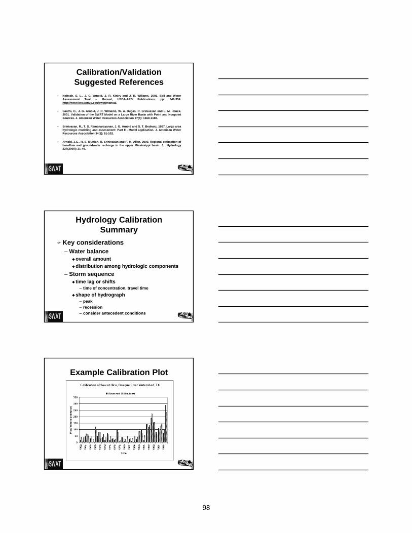
Example Calibration Plot
98
Example Calibration Plot
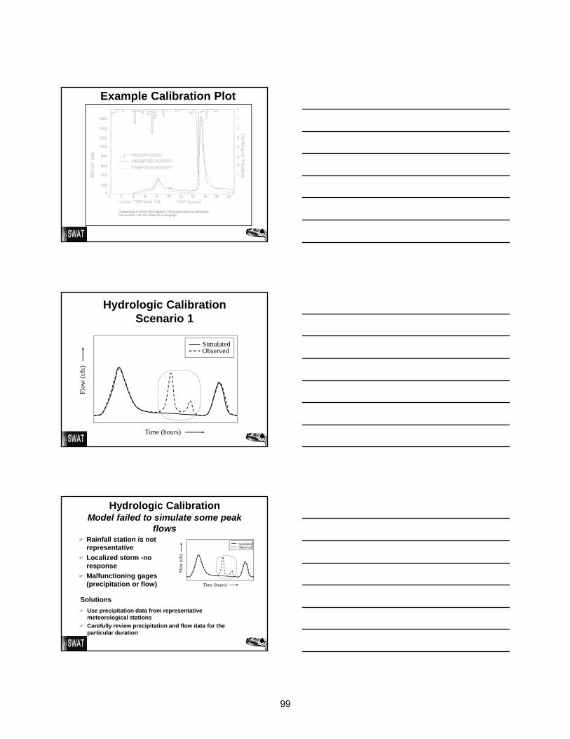
Hydrologic Calibration Scenario 1
SimulatedObserved
Time (hours)
Flow
(cfs
)
Hydrologic CalibrationModel failed to simulate some peak
flows Rainfall station is not
representative
Localized storm -no response
Malfunctioning gages (precipitation or flow)
SimulatedObserved
Time (hours)
Flow
(cfs
)
Use precipitation data from representative meteorological stations
Carefully review precipitation and flow data for the particular duration
Solutions
99
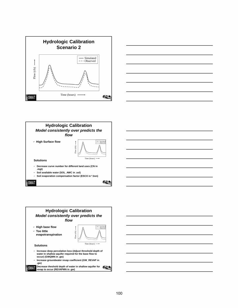
Hydrologic Calibration Scenario 2
SimulatedObserved
Time (hours)
Flow
(cfs
)
Hydrologic CalibrationModel consistently over predicts the
flow
High Surface flow
Decrease curve number for different land uses (CN in .mgt)
Soil available water (SOL_AWC in .sol)
Soil evaporation compensation factor (ESCO in *.bsn)
SimulatedObserved
Time (hours)
Flow
(cfs
)
Solutions
Hydrologic CalibrationModel consistently over predicts the
flow
High base flow
Too little evapotranspiration
Increase deep percolation loss (Adjust threshold depth of water in shallow aquifer required for the base flow to occur) (GWQMN in .gw)
Increase groundwater revap coefficient (GW_REVAP in .gw)
Decrease theshold depth of water in shallow aquifer for revap to occur (REVAPMN in .gw)
SimulatedObserved
Time (hours)
Flow
(cfs
)
Solutions
100
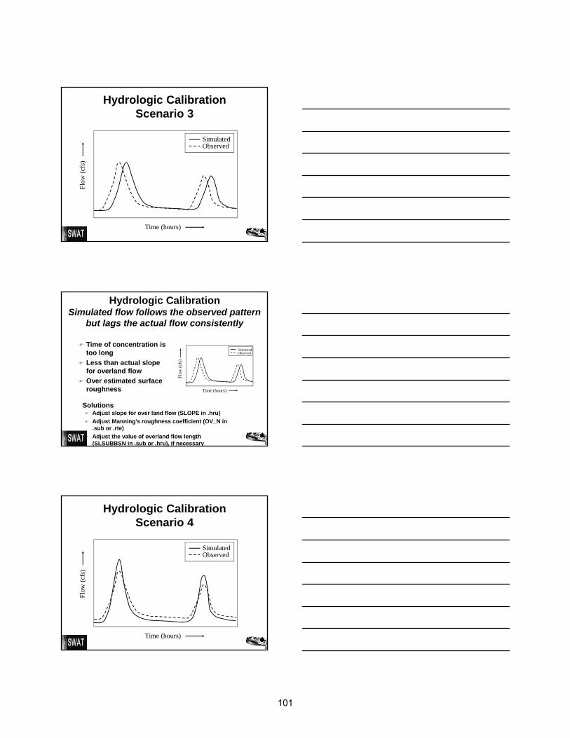
Hydrologic Calibration Scenario 3
SimulatedObserved
Time (hours)
Flow
(cfs
)
Hydrologic CalibrationSimulated flow follows the observed pattern
but lags the actual flow consistently
Time of concentration is too long
Less than actual slope for overland flow
Over estimated surface roughness
Adjust slope for over land flow (SLOPE in .hru)
Adjust Manning’s roughness coefficient (OV_N in .sub or .rte)
Adjust the value of overland flow length (SLSUBBSN in .sub or .hru), if necessary
Solutions
SimulatedObserved
Time (hours)
Flow
(cfs
)
Hydrologic Calibration Scenario 4
SimulatedObserved
Time (hours)
Flow
(cfs
)
101
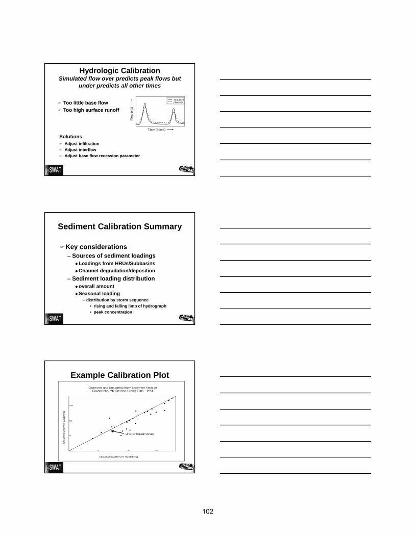
Hydrologic CalibrationSimulated flow over predicts peak flows but
under predicts all other times
Too little base flow
Too high surface runoff
Adjust infiltration
Adjust interflow
Adjust base flow recession parameter
Solutions
SimulatedObserved
Time (hours)Fl
ow (c
fs)
Sediment Calibration Summary
Key considerations– Sources of sediment loadings
Loadings from HRUs/Subbasins
Channel degradation/deposition
– Sediment loading distributionoverall amount
Seasonal loading– distribution by storm sequence
• rising and falling limb of hydrograph
• peak concentration
Example Calibration Plot
102
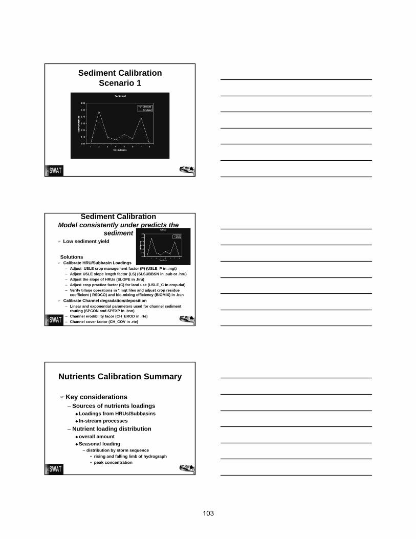
Sediment Calibration Scenario 1
Sediment Calibration Model consistently under predicts the
sediment Low sediment yield
Calibrate HRU/Subbasin Loadings– Adjust USLE crop management factor (P) (USLE_P in .mgt)
– Adjust USLE slope length factor (LS) (SLSUBBSN in .sub or .hru)
– Adjust the slope of HRUs (SLOPE in .hru)
– Adjust crop practice factor (C) for land use (USLE_C in crop.dat)
– Verify tillage operations in *.mgt files and adjust crop residue coefficient ( RSDCO) and bio-mixing efficiency (BIOMIX) in .bsn
Calibrate Channel degradation/deposition– Linear and exponential parameters used for channel sediment
routing (SPCON and SPEXP in .bsn)
– Channel erodibility facor (CH_EROD in .rte)
– Channel cover factor (CH_COV in .rte)
Solutions
Nutrients Calibration Summary
Key considerations– Sources of nutrients loadings
Loadings from HRUs/Subbasins
In-stream processes
– Nutrient loading distributionoverall amount
Seasonal loading– distribution by storm sequence
• rising and falling limb of hydrograph
• peak concentration
103

Example Calibration Plot
Monthly calibration of nitrogen at Hico, Bosque Watershed, TX
Mineral Nitrogen Calibration Scenario 1
Mineral Nitrogen Calibration Model consistently under predicts the
mineral nitrogen Low mineral nitrogen
loading
Calibrate mineral nitrogen loadings– Adjust initial concentration of the nutrient in soils (SOL_NO3 in
.chm)
– Verify fertilizer application rates and adjust fertilizer application fraction to surface layer as 0.20 (FRT_LY1 in .mgt)
– Verify tillage operations in *.mgt files and adjust crop residue coefficient ( RSDCO) and bio-mixing efficiency (BIOMIX) in .bsn
– Adjust nitrogen percolation coefficient (NPERCO in .bsn)
Calibrate in-stream mineral nitrogen processes– Adjust fraction of algal biomass that is as nitrogen for water
quality (AI1 in.wwq)
Solutions
104
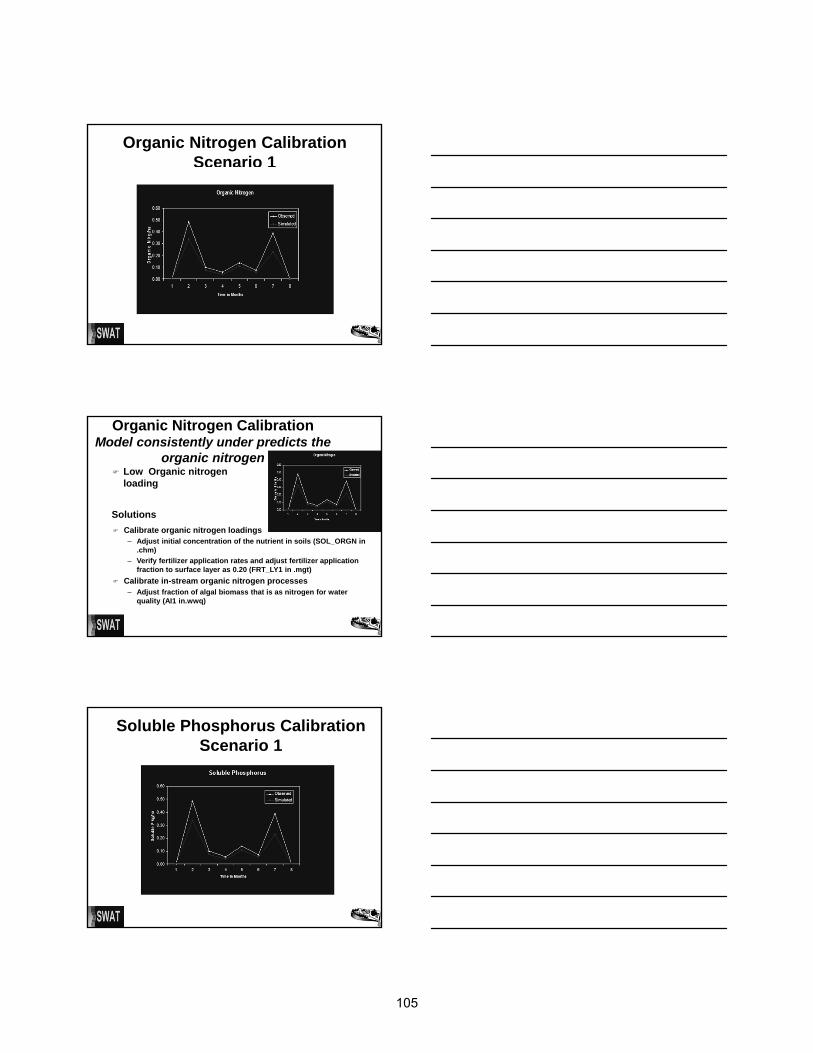
Organic Nitrogen Calibration Scenario 1
Organic Nitrogen Calibration Model consistently under predicts the
organic nitrogen Low Organic nitrogen
loading
Calibrate organic nitrogen loadings– Adjust initial concentration of the nutrient in soils (SOL_ORGN in
.chm)
– Verify fertilizer application rates and adjust fertilizer application fraction to surface layer as 0.20 (FRT_LY1 in .mgt)
Calibrate in-stream organic nitrogen processes– Adjust fraction of algal biomass that is as nitrogen for water
quality (AI1 in.wwq)
Solutions
Soluble Phosphorus Calibration Scenario 1
105
Soluble Phosphorus Calibration Model consistently under predicts the
soluble phosphorus Low soluble phosphorus
loading
Calibrate soluble phosphorus loadings– Adjust initial concentration of the nutrient in soils (SOL_MINP in
.chm)
– Verify fertilizer application rates and adjust fertilizer application fraction to surface layer as 0.20 (FRT_LY1 in .mgt)
– Verify tillage operations in *.mgt files and adjust crop residue coefficient ( RSDCO) and bio-mixing efficiency (BIOMIX) in .bsn
– Adjust phosphorus percolation coefficient (PPERCO in .bsn)
– Adjust phosphorus soil partitioning coefficient (PHOSKD in .bsn)
Calibrate in-stream soluble phosphorus processes– Adjust fraction of algal biomass that is as phosphorus for water
quality (AI2 in.wwq)
Solutions
Organic Phosphorus Calibration Scenario 1
Organic Phosphorus Calibration Model consistently under predicts the
organic phosphorus Low organic phosphorus
loading
Solutions
Calibrate organic phosphorus loadings– Adjust initial concentration of the nutrient in soils (SOL_ORGP in
.chm)
– Verify fertilizer application rates and adjust fertilizer application fraction to surface layer as 0.20 (FRT_LY1 in .mgt)
Calibrate in-stream organic phosphorus processes– Adjust fraction of algal biomass that is as phosphorus for water
quality (AI2 in.wwq)
106
SWAT PuBlicATionSvalidaTiOn Of SWaT On a large river baSin WiTh POinT and nOnPOinT SOurceS
infOrMaTiOn TO run SWaT MOdel
SSurgO PrOceSSing fOr arcSWaT
MOdel evaluaTiOn guidelineS fOr SySTeMaTic quanTificaTiOn Of accuracy in WaTerShed SiMulaTiOnS
Section 4
107

JOURNAL OF THE AMERICAN WATER RESOURCES ASSOCIATIONVOL. 37, NO. 5 AMERICAN WATER RESOURCES ASSOCIATION OCTOBER 2001
VALIDATION OF THE SWAT MODEL ON A LARGE RWERBASIN WITH POINT AND NONPOINT SOURCES1
C. Santhi, J. G. Arnold, J. R. Williams, W. A. Dugas, R. Srinivasan, and L. M. Hauck2
ABSTRACT: The State of Texas has initiated the development of aTotal Maximum Daily Load program in the Bosque River Water-shed, where point and nonpoint sources of pollution are a concern.Soil Water Assessment Tool (SWAT) was validated for flow, sedi-ment, and nutrients in the watershed to evaluate alternative man-agement scenarios and estimate their effects in controllingpollution. This paper discusses the calibration and validation attwo locations, Hico and Valley Mills, along the North Bosque River.Calibration for flow was performed from 1960 through 1998. Sedi-ment and nutrient calibration was done from 1993 through 1997 atHico and from 1996 through 1997 at Valley Mills. Model validationwas performed for 1998. Time series plots and statistical measureswere used to verify model predictions. Predicted values generallymatched well with the observed values during calibration and vali-dation (R2 � 0.6 and Nash-Suttcliffe Efficiency �0.5, in mostinstances) except for some underprediction of nitrogen during cali-bration at both locations and sediment and organic nutrients dur-ing validation at Valley Mills. This study showed that SWAT wasable to predict flow, sediment, and nutrients successfully and canbe used to study the effects of alternative management scenarios.(KEY TERMS: watershed management; total maximum daily load;erosion; sedimentation; phosphorus loading; dairy manure manage-ment.)
INTRODUCTION
The United States Environmental Protection Agen-cy (USEPA) reported nutrient enrichment as themajor cause for impairment of lakes and other waterbodies in the United States (USEPA, 1994). USEPA'swater quality inventory report of 1996 indicated that40 percent of the surveyed rivers, lakes, and estuarieswere polluted relative to their designated uses
(USEPA, 1998). To restore the quality of these waterbodies, the Total Maximum Daily Load (TMDL) pro-cess was established by section 303(d) of the CleanWater Act (CWA). A TMDL quantifies pollutantsources and maximum allowable loads to the con-tributing point and nonpoint sources so that thewater quality standards are attained to protect drink-ing water, aquatic life, and other water uses (USEPA,1998). Once the necessary pollutant reduction levelsare identified through establishment of TMDLs, con-trol measures such as best management practices(BMPs) are to be implemented.
The Texas Natural Resource Conservation Com-mission (TNRCC) is implementing TMDL projects inTexas in cooperation with the Texas State Soil andWater and Conservation Board (TSSWCB). Of the 386classified water bodies, 147 have been listed on the1998 303(d) list. One of these projects is in the BosqueRiver Watershed in North Central Texas, wherephosphorus from confined animal-feeding operationsis a concern (TNRCC, 1999). Runoff from croplandand urban areas (nonpoint sources) and effluent fromwastewater treatment plants (WWTPs) (pointsources) are other pollution sources in this watershed.
Water quality simulation models can assist withTMDL development through simulating loads toreceiving water bodies under various BMPs. Modelsin combination with observational data from histori-cal and current monitoring programs will provide theinformation for TMDL waste/load allocations andimplementation strategies. In this study, the hydro-logic/water quality model, Soil Water Assessment Tool
1Paper No. 00044 of the Journal of the American Water Resources Association. Discussions are open until June 1, 2002.2Respectively, Post Doctoral Research Scientist, Blackland Research Center, 720 East Blackland Road, Temple, Texas 76502-9622;
Hydraulic Engineer, USDA/ARS, 808 East Blackland Road, Temple, Texas 76502; Research Scientist, Blackland Research Center, 720 EastBlackland Road, Temple, Texas 76502-9622; Professor and Resident Director, Blackland Research Center, 720 East Blackland Road, Temple,Texas 76502-9622; Associate Professor and Director of Spatial Sciences Lab, Blackland Research Center, 700 East University Drive, Suite104, College Station, Texas 77840; and Assistant Director, Texas Institute for Applied Environmental Research, P.O. Box T-0410, Stephenville,Texas 76402 (E-MaillSanthi: [email protected]).
JOURNAL OF THE AMERICAN WATER RESOURCES ASSOCIATION 1169 JAWRA
Santhi, Arnold, Williams, Dugas, Srinivasan, and Hauck
(SWAT) was used to study the effect of different BMPsin reducing the pollution. The objective of this paperis to describe the calibration and validation of theSWAT model for flow, sediment, organic, and mineralnutrients in the Bosque River Watershed. The modelwas then used to study the impact of different BMPson the Bosque River Watershed and identify suitableBMPs for achieving water quality targets (Santhi etal., 2000).
SWAT Model Description
SWAT is a hydrologic/water quality model devel-oped by United States Department of Agriculture -Agricultural Research Service (USDA-ARS) (Arnoldet al., 1998). It is a continuous time model that oper-ates on a daily time step. The objective in modeldevelopment was to predict the impact of manage-ment on water, sediment, and agricultural chemicalyields in large ungaged basins. To satisfy the objec-tive, the model (a) is physically based (calibration isnot possible on ungaged basins); (b) uses readilyavailable inputs; (c) is computationally efficient tooperate on large basins in a reasonable time; and(d) is continuous in time and capable of simulatinglong periods for computing the effects of managementchanges. SWAT uses a command structure for routingrunoff and chemicals through a watershed. Com-mands are included for routing flows through streamsand reservoirs, adding flows, and inputting measureddata from wastewater treatment plants. The sub-basin/subwatershed components of SWAT can beplaced into eight major components — hydrology,weather, erosion/sedimentation, soil temperature,plant growth, nutrients, pesticides, and land manage-ment. Erosion and sediment yield are estimated foreach subbasin with the Modified Universal Soil LossEquation (MUSLE) (Williams, 1975). The channelsediment routing equation uses a modification of Bag-nold's sediment transport equation (Bagnold, 1977)that estimates the transport concentration capacity asa function of velocity.
CY = SPCON*VSPEXP (1)
where, CY is sediment transport concentrationcapacity in g/m3; SPCON is the concentration capaci-ty in g/m3 at a velocity of 1 mIs; V is flow velocity inmis; and SPEXP is a constant in Bagnold's equation.The model either deposits excess sediment or re-entrains sediment through channel erosion dependingon the sediment load entering the channel.
The nitrogen processes modeled by SWAT and thevarious pools of nitrogen in the soil are shown in Fig-ure 1 (Arnold et al., 1998; USDA-ARS, 1999). Plantuse of nitrogen is estimated using the supply anddemand approach (Williams et al., 1984). Daily plantdemand is a function of plant biomass and biomass Nconcentration. Available nitrogen in the soil (rootdepth) is supplied to the plant. When demand exceedssupply, there is a nutrient stress. Masses of N03-Ncontained in runoff, lateral flow and percolation areestimated as products of the volume of water and theaverage concentration of nitrate (N03-N) in the soillayer. Organic N transport with sediment is calculat-ed with a loading function developed by McElroy etal. (1976) and modified by Williams and Hann (1978)for application to individual runoff events. The load-ing function estimates daily organic N runoff lossbased on the concentration of organic N in the top soillayer, the sediment yield, and an enrichment ratio(that is, the ratio of organic N in sediment to organicN in soil and typically ranging from two to four). Thephosphorus processes modeled by SWAT and the vari-ous pools of phosphorus in the soil are depicted in Fig-ure 2 (USDA-ARS, 1999). Plant use of phosphorus isestimated using the supply and demand approachsimilar to nitrogen. The loss of dissolved phosphorusin surface runoff is based on the concept of partition-ing pesticides into solution and sediment phases asdescribed by Leonard and Wauchope (1980). Theamount of soluble P removed in :runoff is predictedusing labile P concentration in the top 10 mm of thesoil, the runoff volume and a phosphorus soil parti-tioning factor (that is, the ratio of P attached to sedi-ment to P dissolved in soil water and typical valuesrange from 100 to 175 depending on the soil). Sedi-ment transport of P is simulated with a loading func-tion as described in organic N transport.
Instream nutrient dynamics have been incorporat-ed into SWAT (Ramanarayanan et al., 1996) using thekinetic routines from an instream water qualitymodel, QUAL2E (Brown and Barnwell, 1987). Howev-er, the QUAL2E routines were not explicitly used inthis study. The North Bosque River is a phosphoruslimited system and dominated by large amounts ofattached algae (periphyton) as opposed to suspendedalgae. The in-stream kinetics formulation for SWATdoes not include a periphyton component, a commonlimitation of many in-stream water quality models. Inaddition, inadequate monitoring information exists toquantify the periphyton biomass distribution in theriver. To overcome these limitations, a first-orderdecay kinetic function was developed for the nutrientof concern in the study (phosphorus) and to character-ize the microbial transformation of in-stream solubleP to organic P rather than the more traditionalapproach involving algae growth and phosphorus
MATERIALS AND METHODS
JAWRA 1170 JOURNAL OF THE AMERICAN WATER RESOURCES ASSOCIATION
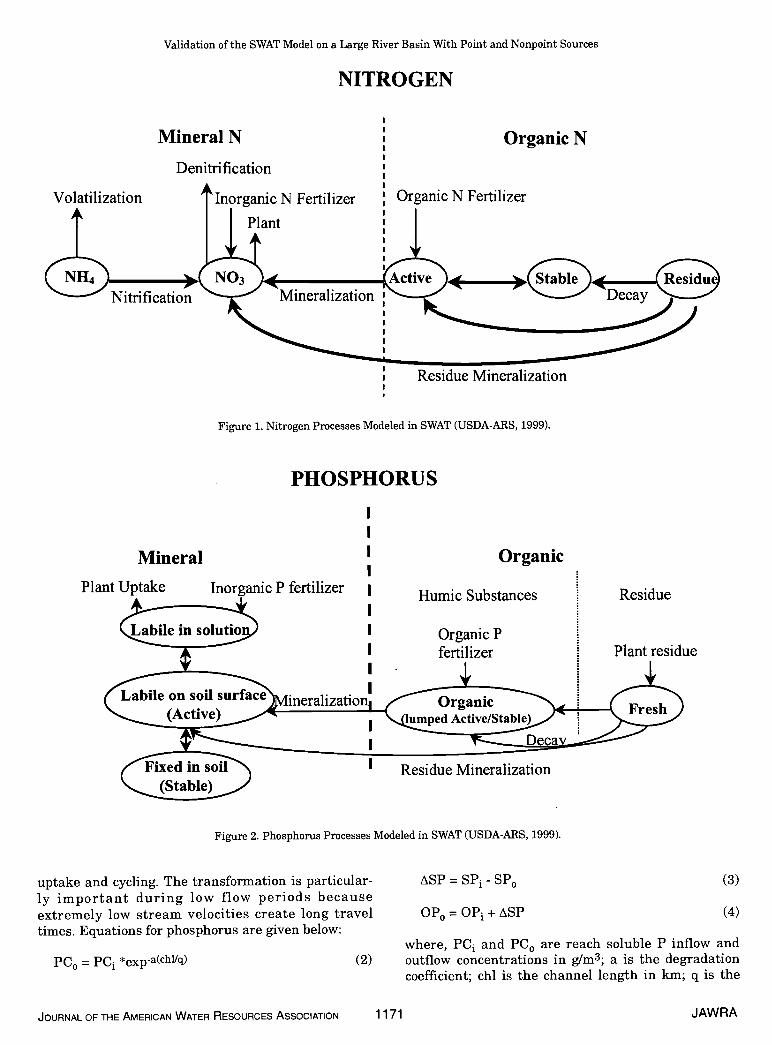
Validation of the SWAT Model on a Large River Basin With Point and Nonpoint Sources
NITROGEN
Mineral N
Denitrification
Organic N
Mineral
Figure 1. Nitrogen Processes Modeled in SWAT (USDA-ARS, 1999).
PHOSPHORUS
Figure 2. Phosphorus Processes Modeled in SWAT (USDA-ARS, 1999).
uptake and cycling. The transformation is particular-ly important during low flow periods becauseextremely low stream velocities create long traveltimes. Equations for phosphorus are given below:
PC0 = PC1 *expa(chllq)
ASP=SP-SP0
OP0 = OP1 + LSP
(3)
(4)
where, PC1 and PC0 are reach soluble P inflow and(2) outflow concentrations in g/m3; a is the degradation
coefficient; chi is the channel length in 1cm; q is the
JOURNAL OF THE AMERICAN WATER RESOURCES ASSOCIATION 1171 JAWRA
Volatilization Fertilizer
Plant
Fertilizer
Nitrification
i Residue Mineralization
Plant Uptake P fertilizer
Organic
I
I
I
Humic Substances
Organic Pfertilizer
Residue
I
Plant residue
Residue Mineralization
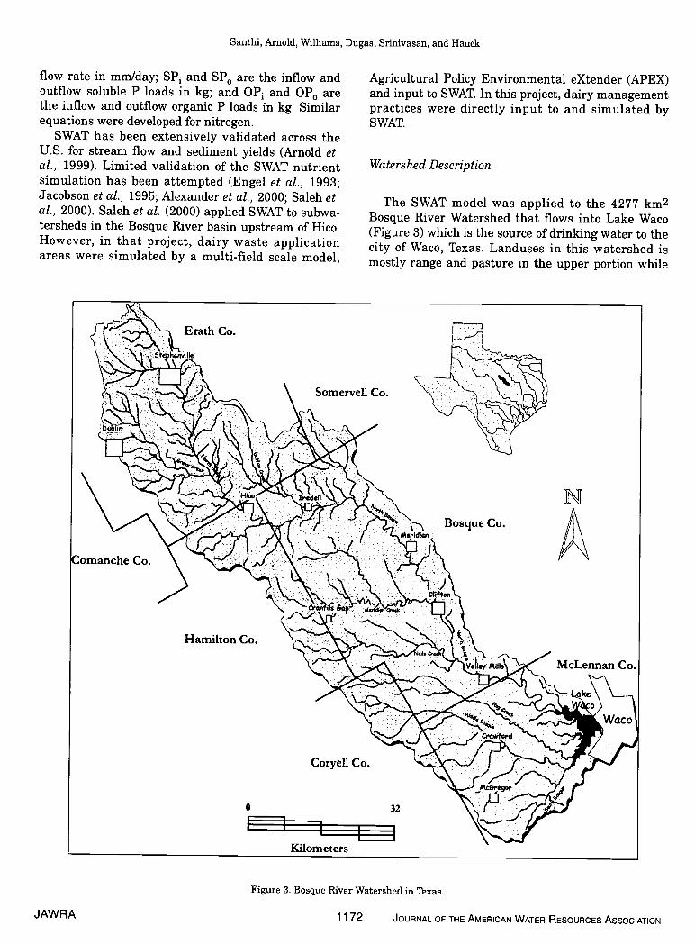
Santhi, Arnold, Williams, Dugas, Srinivasan, and Hauck
flow rate in mmlday; SP and SP0 are the inflow andoutflow soluble P loads in kg; and OP1 and OP0 arethe inflow and outflow organic P loads in kg. Similarequations were developed for nitrogen.
SWAT has been extensively validated across theU.S. for stream flow and sediment yields (Arnold etal., 1999). Limited validation of the SWAT nutrientsimulation has been attempted (Engel et al., 1993;Jacobson et al., 1995; Alexander et al., 2000; Saleh etal., 2000). Saleh et al. (2000) applied SWAT to subwa-tersheds in the Bosque River basin upstream of Hico.However, in that project, dairy waste applicationareas were simulated by a multi-field scale model,
Agricultural Policy Environmental eXtender (APEX)and input to SWAT. In this project, dairy managementpractices were directly input to and simulated bySWAT.
Watershed Description
The SWAT model was applied to the 4277 km2Bosque River Watershed that flows into Lake Waco(Figure 3) which is the source of drinking water to thecity of Waco, Texas. Landuses in this watershed ismostly range and pasture in the upper portion while
Figure 3. Bosque River Watershed in Texas.
JAWRA 1172 JOURNAL OF THE AMERICAN WATER RESOURCES ASSOCIATION
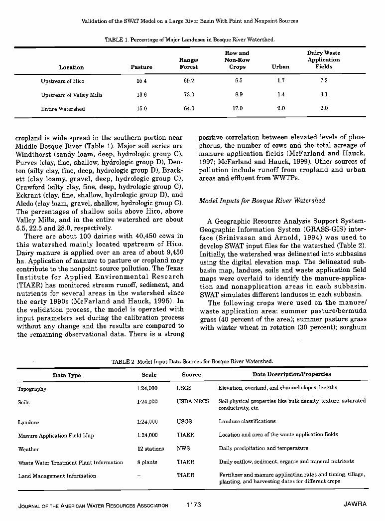
Validation of the SWAT Model on a Large River Basin With Point and Nonpoint Sources
TABLE 1. Percentage of Major Landuses in Bosque River Watershed.
Row and Dairy WasteRangel Non-Row Application
Location Pasture Forest Crops Urban Fields
Upstream of Hico 15.4 69.2 6.5 1.7 7.2
Upstream of Valley Mills 13.6 73.0 8.9 1.4 3.1
Entire Watershed 15.0 64.0 17.0 2.0 2.0
cropland is wide spread in the southern portion near positive correlation between elevated levels of phos-Middle Bosque River (Table 1). Major soil series are phorus, the number of cows and the total acreage ofWindthorst (sandy loam, deep, hydrologic group C), manure application fields (McFarland and Hauck,Purves (clay, fine, shallow, hydrologic group D), Den- 1997; McFarland and Hauck, 1999). Other sources ofton (silty clay, fine, deep, hydrologic group D), Brack- pollution include runoff from cropland and urbanett (clay loamy, gravel, deep, hydrologic group C), areas and effluent from WWTPs.Crawford (silty clay, fine, deep, hydrologic group C),Eckrant (clay, fine, shallow, hydrologic group D), andAledo (clay loam, gravel, shallow, hydrologic group C). Model Inputs for Bosque River WatershedThe percentages of shallow soils above Hico, aboveValley Mills, and in the entire watershed are about A Geographic Resource Analysis Support System-5.5, 22.5 and 28.0, respectively. Geographic Information System (GRASS-GIS) inter-
There are about 100 dairies with 40,450 cows in face (Srinivasan and Arnold, 1994) was used tothis watershed mainly located upstream of Hico. develop SWAT input files for the watershed (Table 2).Dairy manure is applied over an area of about 9,450 Initially, the watershed was delineated into subbasinsha. Application of manure to pasture or cropland may using the digital elevation map. The delineated sub-contribute to the nonpoint source pollution. The Texas basin map, landuse, soils and waste application fieldInstitute for Applied Environmental Research maps were overlaid to identify the manure-applica-(TIAER) has monitored stream runoff, sediment, and tion and nonapplication areas in each subbasin.nutrients for several areas in the watershed since SWAT simulates different landuses in each subbasin.the early 1990s (McFarland and Hauck, 1995). In The following crops were used on the manure!the validation process, the model is operated with waste application area: summer pasture/bermudainput parameters set during the calibration process grass (40 percent of the area); summer pasture grasswithout any change and the results are compared to with winter wheat in rotation (30 percent); sorghumthe remaining Observational data. There is a strong
TABLE 2. Model Input Data Sources for Bosque River Watershed.
Data Type Scale Source Data Description/Properties
Topography 1:24,000 USGS Elevation, overland, and channel slopes, lengths
Soils 1:24,000 USDA-NRCS Soil physical properties like bulk density, texture, saturatedconductivity, etc.
Landuse 1:24,000 USGS Landuse classifications
Manure Application Field Map 1:24,000 TIAER Location and area of the waste application fields
Weather 12 stations NWS Daily precipitation and temperature
Waste Water Treatment Plant Information 8 plants TIAER Daily outflow, sediment, organic and mineral nutrients
Land Management Information — TIAER Fertilizer and manure application rates and timing, tillage,planting, and harvesting dates for different crops
JOURNAL OF THE AMERICAN WATER RESOURCES ASSOCIATION 1173 JAWRA
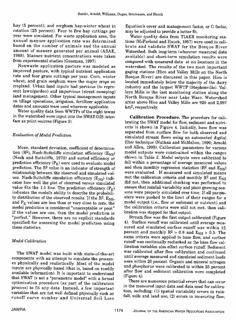
Santhi, Arnold, Williams, Dugas, Srinivasan, and Hauck
hay (5 percent); and sorghum hay-winter wheat inrotation (25 percent). Four to five hay cuttings peryear were simulated. For waste application area, theannual manure application rate was determinedbased on the number of animals and the annualamount of manure generated per animal (ASAE,1988). Manure nutrient concentrations were takenfrom experimental studies (Gassman, 1997).
Nonwaste application pasture was modeled asimproved pasture, with typical nutrient applicationrate and four grass cuttings per year. Corn, winterwheat, and grain sorghum were the major crops oncropland. Urban land inputs had pervious (to repre-sent lawn/garden) and impervious (street sweeping)land management. Other typical management inputson tillage operations, irrigation, fertilizer applicationdates and amounts were used wherever applicable.
Water quality data from WWTPs of the eight townsin the watershed were input into the SWAT-GIS inter-face as point sources (Figure 3).
Evaluation of Model Prediction
Mean, standard deviation, coefficient of determina-tion (R2), Nash-Suttcliffe simulation efficiency (ENS)(Nash and Suttcliffe, 1970) and sorted efficiency orprediction efficiency (RE) were used to evaluate modelprediction. The R2 value is an indicator of strength ofrelationship between the observed and simulated val-ues. Nash-Suttcliffe simulation efficiency (ENS) indi-cates how well the plot of observed versus simulatedvalue fits the 1:1 line. The prediction efficiency (RE)indicates the model's ability to describe the probabili-ty distribution of the observed results. If the R2, ENS,and E values are less than or very close to zero, themodel prediction is considered "unacceptable or poor."If the values are one, then the model prediction is"perfect." However, there are no explicit standardsspecified for assessing the model prediction usingthese statistics.
Model Calibration
The SWAT model was built with state-of-the-artcomponents with an attempt to simulate the process-es physically and realistically. Most of the modelinputs are physically based (that is, based on readilyavailable information). It is important to understandthat SWAT is not a "parametric model" with a formaloptimization procedure (as part of the calibrationprocess) to fit any data. Instead, a few importantvariables that are not well defined physically such asrunoff curve number and Universal Soil Loss
Equation's cover and management factor, or C factor,may be adjusted to provide a better fit.
Water quality data from TIAER monitoring sta-tions (McFarland and Hauck, 1997) were used to cali-brate and validate SWAT for the Bosque RiverWatershed. Both long-term (wherever measured dataavailable) and short-term simulation results werecompared with measured data at six locations in thewatershed. The results of the two most importantgaging stations (Hico and Valley Mills on the NorthBosque River) are discussed in this paper. Hico islocated immediately below the majority of the dairyindustry and the largest WWTP (Stephenville). Val-leys Mills is the last monitoring station along theNorth Bosque River near Lake Waco. Watershedareas above Hico and Valley Mills are 926 and 2,997)p2, respectively.
Calibration Procedure. The procedure for cali-brating the SWAT model for flow, sediment and nutri-ents is shown in Figure 4. Initially, base flow wasseparated from surface flow for both observed andsimulated stream flows using an automated digitalfilter technique (Nathan and McMahon, 1990; Arnoldand Allen, 1999). Calibration parameters for variousmodel outputs were constrained within the rangesshown in Table 3. Model outputs were calibrated tofall within a percentage of average measured valuesand then monthly regression statistics (R2 and ENS)were evaluated. If measured and simulated meansmet the calibration criteria and monthly R2 and ENSdid not, then additional checking was performed toensure that rainfall variability and plant growing sea-sons were properly simulated over time. If all param-eters were pushed to the limit of their ranges for amodel output (i.e., flow or sediment or nutrient) andthe calibration criteria were still not met, then cali-bration was stopped for that output.
Stream flow was the first output calibrated (Figure4). Surface runoff was calibrated until average mea-sured and simulated surface runoff was within 15percent and monthly R2 > 0.6 and ENS > 0.5. Thesame criteria were applied to base flow, and surfacerunoff was continually rechecked as the base flow cal-ibration variables also effect surface runoff. Sedimentwas calibrated after flow calibration and continueduntil average measured and simulated sediment loadswere within 20 percent. Organic and mineral nitrogenand phosphorus were calibrated to within 25 percentafter flow and sediment calibration were completed(Figure 4).
There are numerous potential errors that can occurin the measured input data and data used for calibra-tion, including: (1) spatial variability errors in rain-fall, soils and land use; (2) errors in measuring flow;
JAWRA 1174 JOURNAL OF THE AMERICAN WATER RESOURCES ASSOCIATION
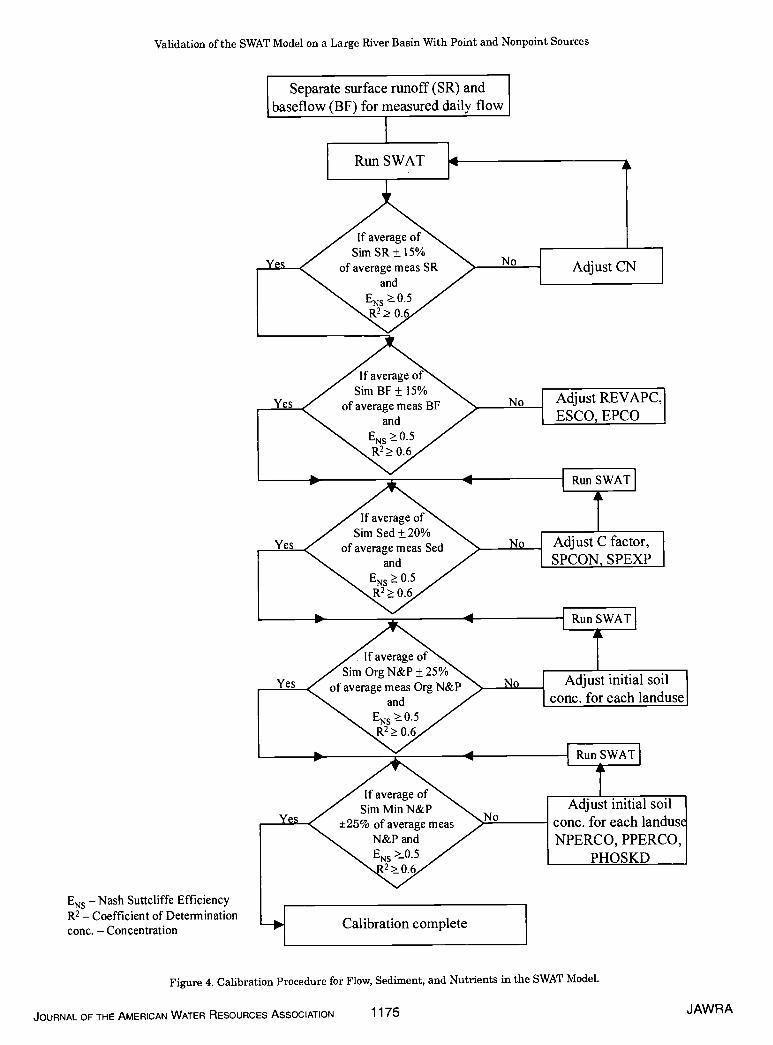
Validation of the SWAT Model on a Large River Basin With Point and Nonpoint Sources
ENS— Nash Suttcliffe Efficiency
R2 — Coefficient of Determinationconc. — Concentration
Figure 4. Calibration Procedure for Flow, Sediment, and Nutrients in the SWAT Model.
JOURNAL OF THE AMERICAN WATER RESOURCES ASSOCIATION 1175 JAWRA
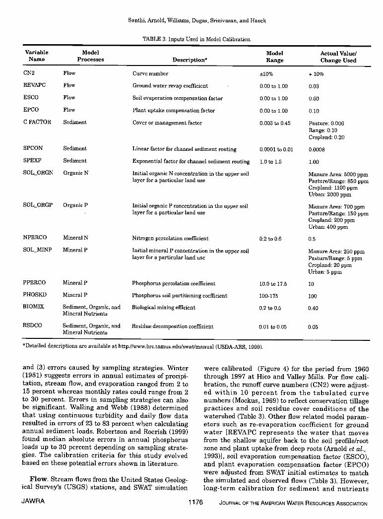
Santhi, Arnold, Williams, Dugas, Srinivasan, and Hauck
TABLE 3. Inputs Used in Model Calibration.
CN2 Flow
REVAPC Flow
ESCO Flow
EPCO Flow
C FACTOR Sediment
SPCON Sediment
SPEXP Sediment
SOL_ORGN Organic N
SOL_ORGP Organic P
NPERCO Mineral N
SOL_MINP Mineral P
PPERCO Mineral P
PHOSKD Mineral P
BIOMIX Sediment, Organic, andMineral Nutrients
RSDCO Sediment, Organic, andMineral Nutrients
Curve number
Ground water revap coefficient
Soil evaporation compensation factor
Plant uptake compensation factor
Cover or management factor
Linear factor for channel sediment routing
Exponential factor for channel sediment routing
Initial organic N concentration in the upper soillayer for a particular land use
Initial organic P concentration in the upper soillayer for a particular land use
Nitrogen percolation coefficient
Initial mineral P concentration in the upper soillayer for a particular land use
Phosphorus percolation coefficient
Phosphorus soil partitioning coefficient
Biological mixing efficient
Residue decomposition coefficient
±10% + 10%
0.00 to 1.00 0.03
0.00 to 1.00 0.60
0.00 to 1.00 0.10
0.003 to 0.45 Pasture: 0.006Range: 0.10Cropland: 0.20
0.0001 to 0.01 0.0008
1.0 to 1.5 1.00
Manure Area: 5000 ppmPasture/Range: 850 ppmCropland: 1100 ppmUrban: 2000 ppm
Manure Area: 700 ppmPasture/Range: 150 ppmCropland: 200 ppmUrban: 400 ppm
Manure Area: 250 ppmPasture/Range: 5 ppmCropland: 20 ppmUrban: 5 ppm
*Detailed descriptions are available at http:llwww.brc.tamus.edulswatJmanual (USDA-ARS, 1999).
and (3) errors caused by sampling strategies. Winter(1981) suggests errors in annual estimates of precipi-tation, stream flow, and evaporation ranged from 2 to15 percent whereas monthly rates could range from 2to 30 percent. Errors in sampling strategies can alsobe significant. Walling and Webb (1988) determinedthat using continuous turbidity and daily flow dataresulted in errors of 23 to 83 percent when calculatingannual sediment loads. Robertson and Roerish (1999)found median absolute errors in annual phosphorusloads up to 30 percent depending on sampling strate-gies. The calibration criteria for this study evolvedbased on these potential errors shown in literature.
Flow. Stream flows from the United States Geolog-ical Survey's (USGS) stations, and SWAT simulation
were calibrated (Figure 4) for the period from 1960through 1997 at Hico and Valley Mills. For flow cali-bration, the runoff curve numbers (CN2) were adjust-ed within 10 percent from the tabulated curvenumbers (Mockus, 1969) to reflect conservation tillagepractices and soil residue cover conditions of thewatershed (Table 3). Other flow related model param-eters such as re-evaporation coefficient for groundwater [REVAPC represents the water that movesfrom the shallow aquifer back to the soil profile/rootzone and plant uptake from deep roots (Arnold et al.,1993)], soil evaporation compensation factor (ESCO),and plant evaporation compensation factor (EPCO)were adjusted from SWAT initial estimates to matchthe simulated and observed flows (Table 3). However,long-term calibration for sediment and nutrients
Variable Model Model Actual Value/Name Processes Description* Range Change Used
0.2 to 0.6 0.5
10.0 to 17.5 10
100-175 100
0.2 to 0.5 0.40
0.01 to 0.05 0.05
JAWRA 1176 JOURNAL OF THE AMERICAN WATER RESOURCES ASSOCIATION
Validation of the SWAT Model on a Large River Basin With Point and Nonpoint Sources
could not be done, as observed data were not avail-able.
The model was then run from 1990 through 1998for calibrating sediment and nutrients as per avail-ability of the monitored data. Calibration of sedimentand nutrient loads (kg/ha) were conducted for Hicofrom 1993 through 1997 and for Valley Mills from1996 through 1997 on a monthly basis. The simula-tion was started from 1990 to reduce errors in initialestimates of state variables such as soil water contentand surface residue.
Sediment. The cover, or C factor, of the UniversalSoil Loss Equation for range and pasture was adjust-ed to match observed and simulated sediment loads(Figure 4). The C factor was adjusted (Table 3) to rep-resent the surface cover better in the range and pas-ture lands. Channel sediment routing variables suchas the linear factor for calculating the maximumamount of sediment reentrained during channel sedi-ment routing (SPCON) and the exponential factor forcalculating the sediment reentrained in the channelsediment routing (SPEXP) were also adjusted (Table3) during the sediment calibration. These two vari-ables were adjusted to represent the cohesive natureof the channels in this watershed (Allen et al., 1999).
Organic Nutrients. Initial concentrations oforganic nitrogen and phosphorus in the soil upper lay-ers (SOL_ORGN and SOL_ORGP) for different lan-duses are available in the soil database table(USDA-ARS, 1999). However, these values wererefined/modified to suit each landuse condition in thiswatershed (Table 3 and Figure 4).
Mineral Nutrients. SWAT estimates the initialconcentration for mineral N (Mm N) based on the soilproperties at individual subbasins. Therefore, noadjustments were made to initial concentration of mmN. Nitrogen percolation coefficient (NPERCO) wasadjusted from initial value of SWAT to match thiswatershed condition (Table 3 and Figure 4). Initialconcentration for mineral P (mm P) in the soil upperlayer (SOL_MINP) for different landuse was set atappropriate levels based on available literature(Gassman, 1997; A. N. Sharpley, USDA-ARS, Durant,Oklahoma, and L. M. Hauck, TIAER, Stephenville,Texas, personal communication, 1998). Other mm Prelated coefficients such as phosphorus percolationcoefficient (PPERCO) and phosphorus soil partition-ing coefficient (PHOSKD) were initialized at accept-able levels (Table 3 and Figure 4) to suit theconditions of the watershed (L. M. Hauck, TIAER,Stephenville, Texas, personal communication, 1998).The residue decomposition coefficient (RSDCO) andbiological mixing efficiency (BIOMIX) were also
adjusted (Table 3). The initial values of most of thesevariables are already set at default values in theSWAT model. They were refined during the calibra-tion to suit the Bosque River Watershed conditions.
Model Validation
In the validation process, the model is operatedwith input parameters set during the calibration pro-cess without any change and the results are comparedto the remaining observational data to evaluate themodel prediction. Measurements for January throughDecember 1998 were used to validate the model forHico and Valley Mills. The same statistical measureswere used to assess the model prediction.
Best Management Practices
The calibrated model was used to study the long-term effects of various BMPs related to dairy manuremanagement and municipal wastewater treatmentplant loads in this watershed. Among several scenar-ios studied, four scenarios are discussed in this paper.Detailed description of the BMPs can be found in San-thi et al. (2000). The existing condition scenario simu-lates the watershed under existing conditions such aspresent dairy herd size, present waste applicationfields (WAF) areas, average manure application rate(13 tfha/yr), present discharge volumes from WWTPswith current median concentrations for nutrients, andpresent urban and cropland areas (Table 4). Thefuture condition scenario reflects the projected condi-tions of the watershed in year 2020 such as projecteddairy herd size (67,000), manure application in WAFsat the crop nitrogen requirement rate (N rate at 46tlha/yr), WAF area calculated at N rate requirement,maximum permitted discharge volumes from WWTPsusing nutrient concentrations defined by currentmedian values, urban area increased by 30 percent toreflect the projected population growth in 2020, andcropland area at current levels (due to no increase incropland over last two decades) (Table 4). Three addi-tional WWTPs with 1 mg/l concentration of total Pwere input into the model as point sources along theNorth Bosque River to account for possible industrialfuture growth outside existing communities.
Several management practices on dairy manureand WWTP effluents were simulated to study theimpact in reducing the mm P loadings. Dairy manage-ment practices such as hauling of the solid manurefrom watershed, application of manure at crop Prequirement rate (P rate) at 6.3 t/halyr (as N rateallows excess application of P than crop required),
JOURNAL OF THE AMERICAN WATER RESOURCES ASSOCIATION 1177 JAWRA
Santhi, Arnold, Williams, Dugas, Srinivasan, and Hauck
TABLE 4. Assumptions of BMP Scenarios.
ScenarioWWTP Flow
PeriodWWTPP Limit
DairyManure
ApplicationRate
ReducedP in Diet
ManureHaul Off
Existing 1997-1998 (actual) Median Concentration Btw N&P Rate No No
Future 2020 (permitted) Median Concentration N Rate No No
Scenario E 1997-1998 All WWTPs at Median Concentrationand Stephenville WWTP — 1 mg/l
P Rate Yes Yes
Scenario F 2020 All WWTPs with Loads Equal toScenario E and Stephenville WWTP—With load equal to 1 mg/i of future
P Rate Yes Yes
and reduction of the dairy diet P to 0.4 percent(results in reducing the dairy manure P content by 29percent as suggested by Keplinger, 1999) wereimposed. The concentrations of total P in WWTPeffluents were reduced to 1 mg/l.
Scenario E was a modification of the existing con-dition scenario with additional conditions imposed onmanure application rate (P rate), hauling off 38 per-cent of the manure, P diet reduction in animal feed,and 1 mgfl limits of P in WWTPs (Table 4). Scenario Fwas a modification over the future scenario withmanure applied at P rate, hauling off 38 percent ofthe manure, P diet reduction, and 1 mg/I P limits onall WWTPs.
RESULTS AND DISCUSSION
Model Calibration
Flow. Measured and simulated annual flows atHico and Valley Mills matched well (Figures 5a and5b). Monthly simulated and observed flows during thenutrient calibration at the two locations matched well(Figures 6a and 7a). Means and standard deviationsof the observed and simulated flows for long-term andshort-term at Hico and Valley Mills were within a dif-ference of 10 percent (Tables 5 and 6). Further agree-ment between observed and simulated flows at Hicoand Valley Mills are shown by the coefficient of deter-minations greater than 0.6, ENS and E valuesgreater than 0.72 (Tables 5 and 6). The estimated pro-portions of base flow from the observed flows at Hicoand Valley Mills were 30 percent and 34 percent fromthe filter technique. They were 28 percent and 27 per-cent for the same locations for SWAT simulated flows.These results for surface runoff and base flow for
observed and simulated flows reveal that hydrologicprocesses in SWAT are modeled realistically and theconcentrations at all flow regimes are realistic.
Sediment. The temporal variations of sedimentloading at Hico and Valley Mills are represented inFigures 6b ad 7b. There is a significant R2 relation-ship between observed and simulated sediments bothat Hico and Valley Mills (R2 � 0.81). The values ofENS for Hico and Valley Mills above 0.69 indicate thatthe simulated sediment is closer to the observed sedi-ment. The E values at Hico and Valley Mills indicatethat model explained the probability distribution ofthe observed sediments well (Tables 5 and 6).
Organic Nutrients. Monthly loadings of organicnitrogen and phosphorus (Org N and org P) for Hicoand Valley Mills are shown in Figures 6c, 6d, 7c and7d. Mean and standard deviation for observed andsimulated org N are within 10 percent of difference atHico (Table 5). The R2 value indicated that observedand simulated values were closer and ENS indicatedthat the observed versus simulated plot was close to1:1. There were under prediction of loads during a fewmonths in early 1993 and middle of 1997 (Figure 6c).At Valley Mills, simulated org N was much closer toobserved org N (Table 6). At Hico and Valley Mills,the values of simulated and observed org P were clos-er (Tables 5 and 6). The deviations of the simulatedvalues were closer to their mean compared to theobserved values.
Mineral Nutrients. The temporal patterns ofobserved and simulated mm N and P for Hico(Figures 6e and 6f) and statistics indicated that pre-dictions of Mm N and P at Hico corresponded wellwith the observed values (Table 5). However, themodel overpredicted the mm N at Valley Mills during
JAWRA 1178 JOURNAL OF THE AMERICAN WATER RESOURCES ASSOCIATION
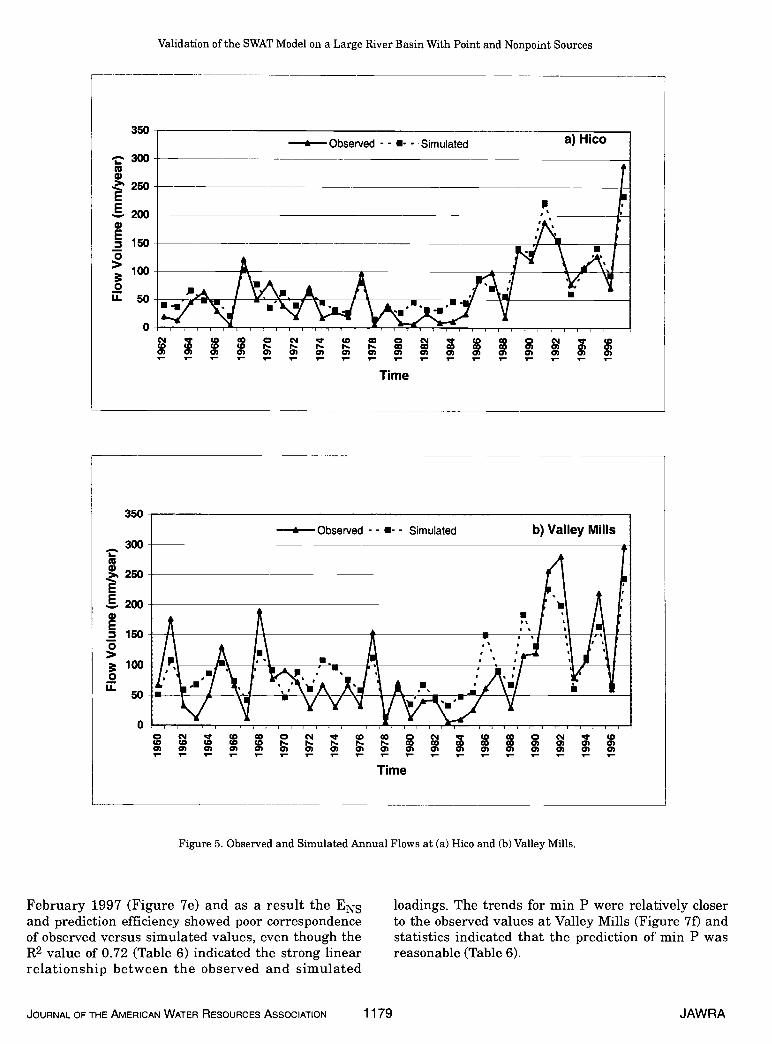
Validation of the SWAT Model on a Large River Basin With Point and Nonpoint Sources
Figure 5. Observed and Simulated Annual Flows at (a) Hico and (b) Valley Mills.
February 1997 (Figure 7e) and as a result the ENSand prediction efficiency showed poor correspondenceof observed versus simulated values, even though theR2 value of 0.72 (Table 6) indicated the strong linearrelationship between the observed and simulated
loadings. The trends for mm P were relatively closerto the observed values at Valley Mills (Figure 7f) andstatistics indicated that the prediction of mm p wasreasonable (Table 6).
JOURNAL OF THE AMERICAN WATER RESOURCES ASSOCIATION 1179 JAWRA
£ Observed - - U- - Simulated a) Hico350
300(5
250
200E _____________ ________ ________________________1500> ______________________ __________________________0LL. 50
0C . CD CD C C1 CD CD C C'l CD CD 0 C CDCD CD CD CD l- 1'- r-.. N.. CD CD CD CD CD CD CD CD CDCD CD CD CD CD CD CD CD CD CD CD CD CD CD CD CD CD CD— — — — 1 - — .- 1- 1
Time
350
300
250
.200
150
1000
LI.50
0 O N CD CD 0 N CD CD 0 N CD CD 0 N CDCD CD CD CD CD N. F— F-- N.. N.. CD CD CD CD CD CD CD CD CDCD CD CD CD CD CD CD CD CD CD CD CD CD CD CD CD CD CD CD, — — I 1 r , — 1 1 1 1
Time
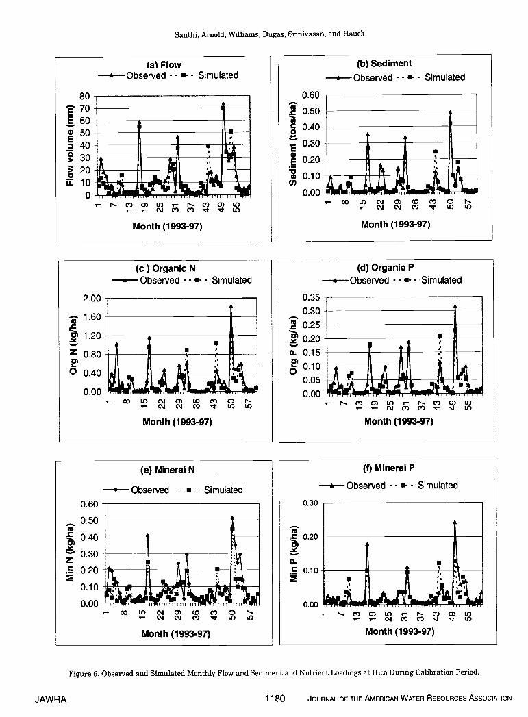
_. 0.50'U.
0.30
.E 0.20
0.10
Santhi, Arnold, Williams, Dugas, Srinivasan, and Hauck
Figure 6. Observed and Simulated Monthly Flow and Sediment and Nutrient Loadings at Hico During Calibration Period.
JAWRA 1180 JOURNAL OF THE AMERICAN WATER RESOURCES ASSOCIATION
(ati Flow£ Observed - - .- - Simulated
fl———
-H1LJ I .
80
60 ___ _______• 5040
0 _______ _______________
20
1
(b) Sediment. Observed - - .- - Simulated
0.60(U.c 0.50
0.40
— 0.30'U _______ _______________ ____0.20
• 0.10Cl)
0.00CO U) CJ 0) (0 C) 0 N.1 CJ C\J C') LI) U)
Month (1993-97)
I
aAJ.fMonth (1 993-97)
(c ) Organic N£ Observed - - .- - Simulated
2.00
1.60
1.20
Z 0.80
0.40
0.00
(d) Organic P£ Observed - - .- - Simulated
0.35
0.30(U ____-C
a- 0.15
0.10
0.05
0.00 inii.N-. C') 0) U) N- C') 0) U)1 C')C') LI)
Month (1993-97)
(0 LI) CJ 0) (0 C') ON.'- C'J C'i C') U) LI)
Month (1 993-97)
(e) Mineral N
0.60
• Observed -. u Simulated
(f) Mineral P
a. Observed - - - - Simulated
0.30
0.00
0.20
. 0.10
CO LI) CJ 0) (DC') ON.'- C'J C'J C') U) U)
Month (1993-97)
0.00N- C') 0) U),- N. C') 0) U)i-i- C\J C') C') U)
Month (1 993-97)
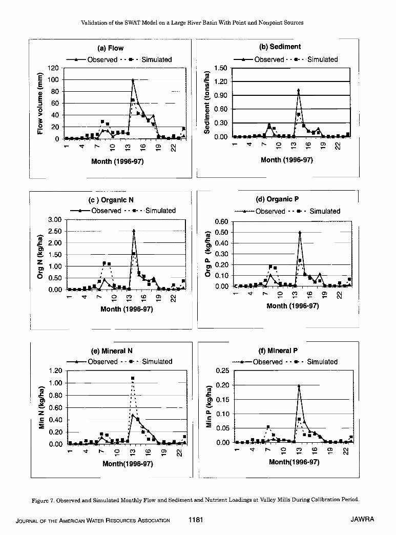
Validation of the SWAT Model on a Large River Basin With Point and Nonpoint Sources
120
600> 40220U-
0
(a) Flow.' Observed - - - - 'Simulated
Month (1996-97) Month (1996-97)
Figure 7. Observed and Simulated Monthly Flow and Sediment and Nutrient Loadings at Valley Mills During Calibration Period.
JOURNAL OF THE AMERICAN WATER RESOURCES ASSOCIATION 1181 JAWRA
(b) Sediment
£ Observed - - .- - Simulated1.50
-C
C0
0.60E
0.30Cl)
0.00
A•,___Urhh1r/9jUj
'- N- 0 C) (0 0) C.J1 ¶ C%J
. N- 0 C) CD 0) CJ'- '— '— - cJ
(d) Organic P£ Observed - - .- - 'Simulated
(C ) Organic N£ Observed - - .- - 'Simulated
3.00
2.50 ——-—— —________
2.00
..1.501.00 :'
00.50 •0.00 I I I I I IUIAII1'
'- N- 0 C) (0 0) CJ1 • • T C'JMonth (1996-97)
0.60
0.50-C• 0.40
0.30
0.20
0 0.100.00 N- 0 C) (0 0) CsJ.- 1 • • CJ
Month (1 996-97)
1.20
(e) Mineral N£ Observed - - - Simulated
1.00
0.80
' 0.60z. 0.40
0.20
0.00
0.25
(t) Mineral Pa Observed - - .- - 'Simulated
_. 0.20
0.15
0.10
0.05
'- N- 0 C) (0 0) Ci_ 1 • ('1Month(1 996-97)
0.00r
— _k__.•__ !
'- N- 0 C) CD 0) CJ'- '- ,_ ¶ C.J
Month(1 996-97)
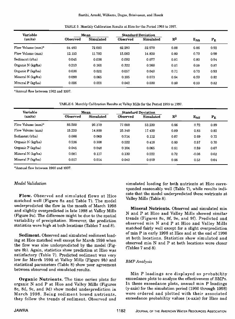
Santhi, Arnold, Williams, Dugas, Srinivasan, and Hauck
TABLE 5. Monthly Calibration Results at Hico for the Period 1993 to 1997.
Variable Mean Standard Deviation(units) Observed Simulated Observed Simulated R2 ENS PE
Flow Volume (mm)* 64.460 72.090 62.280 52.970 0.88 0.86 0.92
Flow Volume (mm) 12.110 11.790 15.060 14.820 0.80 0.79 0.99
Sediment (tiha) 0.045 0.038 0.092 0.077 0.81 0.80 0.94
Organic N (kg/ha) 0.213 0.161 0.322 0.260 0.61 0.58 0.87
Organic P (kg/ha) 0.036 0.031 0.057 0.049 0.71 0.70 0.93
Mineral N (kg/ha) 0.090 0.065 0.105 0.073 0.64 0.59 0.82
Mineral P (kg/ha) 0.026 0.021 0.042 0.030 0.60 0.59 0.83
*kmual flow between 1962 and 1997.
TABLE 6. Monthly Calibration Results at Valley Mills for the Period 1993 to 1997.
Variable Mean Standard Deviation(units) Observed Simulated Observed Simulated R2 ENS E
Flow Volume (mm)* 86.500 92.310 77.050 53.230 0.66 0.72 0.89
Flow Volume (mm) 15.220 14.800 25.340 17.420 0.89 0.83 0.85
Sediment (t/ha) 0.086 0.069 0.214 0.112 0.87 0.69 0.72
Organic N (kg/ha) 0.236 0.308 0.522 0.418 0.60 0.57 0.70
Organic P (kg/ha) 0.045 0.048 0.104 0.065 0.61 0.59 0.67
Mineral N (kg/ha) 0.081 0.117 0.130 0.222 0.72 -0.08 0.03
Mineral P (kg/ha) 0.017 0.014 0.042 0.019 0.66 0.53 0.64
flow between 1960 and 1997.
Model Validation
Flow. Observed and simulated flows at Hicomatched well (Figure 8a and Table 7). The modelunderpredicted the flow in the month of March 1998and slightly overpredicted in late 1998 at Valley Mills(Figure 9a). The difference might be due to the spatialvariability of precipitation. However, the predictionstatistics were high at both locations (Tables 7 and 8).
Sediment. Observed and simulated sediment load-ing at Hico matched well except for March 1998 whenthe flow was also underpredicted by the model (Fig-ure 8b). Again, statistics show prediction at Hico wassatisfactory (Table 7). Predicted sediment was verylow for March 1998 at Valley Mills (Figure 9b) andstatistical parameters (Table 8) show poor agreementbetween observed and simulated results.
Organic Nutrients. The time series plots fororganic N and P at Hico and Valley Mills (Figures8c, 8d, 9c, and 9d) show model underprediction inMarch 1998. Being sediment bound nutrients,they follow the trends of sediment. Observed and
simulated loading for both nutrients at Hico corre-sponded reasonably well (Table 7), while results indi-cate that the model underpredicted these nutrients atValley Mills (Table 8).
Mineral Nutrients. Observed and simulated mmN and P at Hico and Valley Mills showed similartrends (Figures 8e, 8f, 9e, and 90. Predicted andobserved mm N and P at Hico and Valley Millsmatched fairly well except for a slight overpredictionof mm in early 1998 at Hico and at the end of 1998at both locations. Statistics show simulated andobserved mm N and P at both locations were closer(Tables 7 and 8).
BMP Analysis
Mm p loadings are displayed as probabilityexceedance plots to analyze the effectiveness of BMPs.In these exceedance plots, annual mm P loadings(y-axis) for the simulation period (1960 through 1998)were ordered and plotted with their associatedexceedance probability values (x-axis) for Hico and
JAWRA 1182 JOURNAL OF THE AMERICAN WATER RESOURCES ASSOCIATION
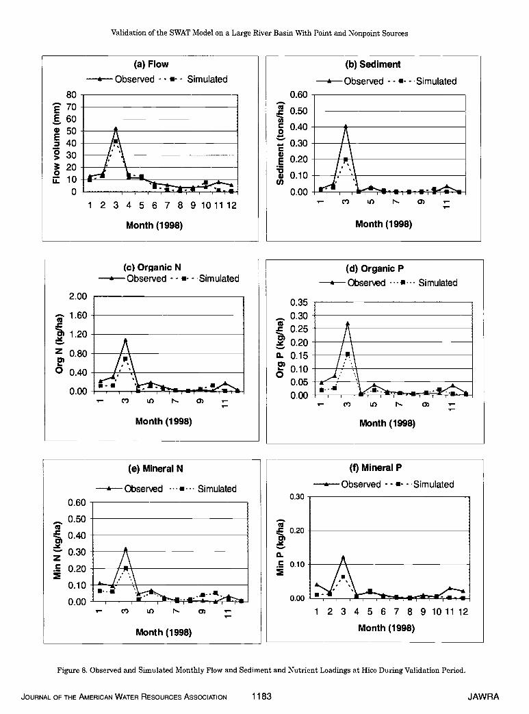
2.00
1.60
zo 0.40
1.20
0.80
Validation of the SWAT Model on a Large River Basin With Point and Nonpoint Sources
Figure 8. Observed and Simulated Monthly Flow and Sediment and Nutrient Loadings at Hico During Validation Period.
JOURNAL OF THE AMERICAN WATER RESOURCES ASSOCIATION 1183 JAWRA
(a) Flow£ Observed - •- - Simulated
80
605040
020
100
(b) Sediment
A Observed - - - - Simulated0.60
0.40
0.30
0.20
G) 0.10U)
0.00
1 2 3 4 5 6 7 8 9 101112
Month (1998)
- (Y) ) N- C) i-1
(C) Organic NA Observed - - .-- Simulated
Month (1998)
0.00
0.35
. 0.302 0.25
0.200. 0.15
o.io0.05
0.00
(d) Organic PA Obsened - - s--- Simulated
, ,'.cv) U) N- C)
Month (1998)
- C') U) N- 0) 1Month (1998)
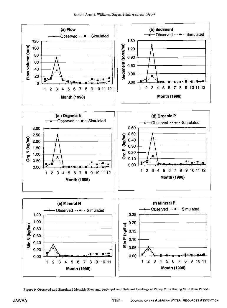
120
180
E 600> 40
200
Santhi, Arnold, Williams, Dugas, Srinivasan, and Hauck
(a) Flow.i Observed - - .- - Simulated
Month (1998)
Figure 9. Observed and Simulated Monthly Flow and Sediment and Nutrient Loadings at Valley Mills During Validation Period.
JAWRA 1184 JOURNAL OF THE AMERICAN WATER RESOURCES ASSOCIATION
(b) Sediment.1 Observed -. .- - Simulated
1.50
E 1.20(lC
0.90
0.60E
0.30Cl)
0.00
1 2 3 4 5 6 7 8 9 10 1112 1 2 3 4 5 6 7 8 9 1011 12
(C ) Organic N£ Observed - - .- - Simulated
Month (1998)
3.00
2.50
2.00
. 1.501.00
0 0.500.00
(d) Organic P•' Observed - - - - Simulated
0.60
0.50
0.40
0.30
0; 0.20I-O 0.10 jIrn. _.u U ! 1—11'0.00
1 2 3 4 5 6 7 8 9 1011 12Month (1998)
1 2 3 4 5 6 7 8 9 101112Month (1998)
(e) Mineral N
£ Observed - - - - Simulated1.20
1.00
0.80
0.60z. 0.40
0.20
0.001 2 3 4 5 6 7 8 9 10 11
Month (1998)
tp •.........I.. .i .
(f) Mineral P£ Observed - - .- - Simulated
0.25
0.20
0.15
0.10
0.05
0.001 2 3 4 5 6 7 8 9 10 11
Month (1998)
A. -.-U-.-. . . •-,i--u-,-I-,-i
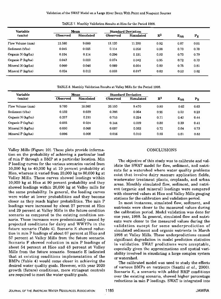
Validation of the SWAT Model on a Large River Basin With Point and Nonpoint Sources
TABLE 7. Monthly Validation Results at Hico for the Period 1998.
Variable(units)
Mean Standard DeviationObserved Simulated Observed Simulated R2 ENS E
Flow Volume (mm) 11.580 9.000 13.120 11.290 0.92 0.87 0.91
Sediment (tlha) 0.045 0.025 0.114 0.056 0.98 0.70 0.70
OrganicN(kg/ha) 0.194 0.114 0.296 0.191 0.92 0.73 0.79
Organic P (kg/ha) 0.043 0.023 0.074 0.042 0.95 0.72 0.73
Mineral N (kg/ha) 0.060 0.046 0.089 0.054 0.89 0.75 0.81
Mineral P (kg/ha) 0.024 0.012 0.033 0.017 0.83 0.53 0.62
TABLE 8. Monthly Validation Results at Valley Mills for the Period 1998.
Variable(units)
Mean Standard DeviationObserved Simulated Observed Simulated R2 ENS E
Flow Volume (mm) 9.760 10.980 20. 150 9.470 0.80 0.62 0.63
Sediment (tlha) 0.132 0.039 0.386 0.064 0.95 0.23 0.23
Organic N (kg/ha) 0.257 0.211 0.715 0.224 0.71 0.43 0.44
Organic P (kg/ha) 0.055 0.034 0.144 0.039 0.80 0.39 0.41
Mineral N (kg/ha) 0.050 0.068 0.097 0.063 0.72 0.64 0.73
Mineral P (kg/ha) 0.006 0.008 0.016 0.010 0.93 0.81 0.83
Valley Mills (Figure 10). These plots provide informa-tion on the probability of achieving a particular loadof mm P through a BMP at a particular location. MmP loading curves for the various scenarios varied from10,000 kg to 40,000 kg at 10 percent probability atHico, whereas it varied from 20,000 kg to 80,000 kg atValley Mills. These curves showed loadings within10,000 kg at Hico at 90 percent probability and theyshowed loadings within 20,000 kg at Valley mills forthe same probability. In general, the loading curveswere wider at lower probabilities and they becomecloser as they reach higher probabilities. The mm ploadings were increased by about 27 percent at Hicoand 29 percent at Valley Mills in the future conditionscenario as compared to the existing condition sce-nario. These increases were predominantly caused byprojected conditions for dairy and WWTPs in thefuture scenario (Table 4). Scenario E showed reduc-tion in mm P loadings of about 67 percent at Hico and57 percent at Valley Mills from the future scenario.Scenario F showed reduction in mm P loadings ofabout 54 percent at Hico and 48 percent at ValleyMills from the future scenario. Scenario E indicatedthat at existing conditions implementation of theBMPs (Table 4) would come closer in achieving thedesired water quality goals. However, with year 2020growth (future) conditions, more stringent controlsare required to meet the water quality goals.
CONCLUSIONS
The objective of this study was to calibrate and val-idate the SWAT model for flow, sediment, and nutri-ents for a watershed where water quality problemsexist that involve dairy manure application fields,wastewater treatment plants, croplands, and urbanareas. Monthly simulated flow, sediment, and nutri-ent (organic and mineral) loadings were comparedwith observed values at Hico and Valley Mills gaugingstations for the calibration and validation period.
In most instances, simulated flow, sediment, andnutrients were closer to the measured values duringthe calibration period. Model validation was done forone year, 1998. In general, simulated flow and nutri-ents were closer to the measured values during thevalidation except for some underprediction ofsimulated sediment and organic nutrients in March1998 at Valley Mills. These underpredictions causedsignificant degradation in model prediction statisticsin validation. SWAT predictions were acceptable,especially given the approximations and spatial vari-ability involved in simulating a large complex systemor watershed.
The calibrated model was used to study the effectsof various BMPs on nutrients (Santhi et al., 2000).Scenario E, a scenario with added BMP conditionsover the existing scenario, showed higher percentagereductions in mm loadings. SWAT is integrated into
JOURNAL OF THE AMERICAN WATER RESOURCES ASSOCIATION 1185 JAWRA
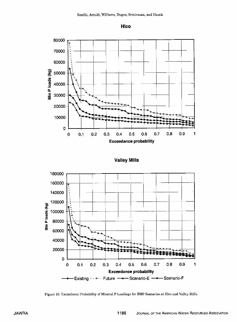
80000
70000
60000
40000
30000
20000
10000
0
Hico
1
Santhi, Arnold, Williams, Dugas, Srinivasan, and Hauck
50000U)V0a.C
0 0.1 0.2 0.3 0.4 0.5 0.6 0.7 0.8 0.9
Exceedance probability
Valley Mills
1
180000
160000
140000
. 120000C)
. 1000000a. 80000
60000
40000
20000
00 0.1 0.2 0.3 0.4 0.5 0.6 0.7 0.8 0.9
Exceedance probability• Existing - - +- - Future £ Scenario-E • Scenario-F
Figure 10. Exceedance Probability of Mineral P Loadings for BMP Scenarios at Hico and Valley Mills.
JAWRA 1186 JOURNAL OF THE AMERICAN WATER RESOURCES ASSOCIATION
Validation of the SWAT Model on a Large River Basin With Point and Nonpoint Sources
the USEPA's watershed modeling framework, calledBASINS and is expected to be used by many state andfederal agencies. The SWAT calibration and valida-tion procedures presented in this paper will be usefulto researchers and engineers involved in studyingwater quality problems.
ACKNOWLEDGMENTS
The authors would like to acknowledge the USDA and TexasInstitute for Applied Environmental Research, Stephenville, Texas,for providing funding for this research work.
LITERATURE CITED
Alexander, R. B., R. A. Smith, G. E. Schwarz, S. D. Stephen Pre-ston, J. W. Brakebill, R. Srinivasan, and P. Percheo, 2000. Atmo-spheric Nitrogen Flux from the Fluvial Drainages of MajorEstuaries in the United States and Application of the SPAR-ROW Watershed Model. Draft of the chapter to be published bythe American Geophysical Union on Assessing the RelativeNitrogen Inputs to Coastal Waters from the Atmosphere.
Allen, P. M., J. G. Arnold, and E. Jakubowski, 1999. Prediction ofStream Channel Erosion Potential. Environmental and Engi-neering Geoscience 3:339-35 1.
Arnold, J. G. and P. M. Allen, 1999. Automated Methods for Esti-mating Baseflow and Groundwater Recharge from Stream FlowRecords. Journal of American Water Resources Association35(2):411-424.
Arnold, J. G., P. M. Allen, and G. Bernhardt, 1993. A Comprehen-sive Surface-Groundwater Flow Model. Journal of Hydrology142(1993):47-69.
Arnold, J. G., R. Srinivasan, R. S. Muttiah, and P. M. Allen, 1999.Continental Scale Simulation of the Hydrologic Balance. Jour-nal of American Water Resources Association 35(5):1037-1051.
Arnold, J. G., R. Srinivasan, R. S. Muttiah, and J. R. Williams,1998. Large Area Hydrologic Modeling and Assessment Part I:Model Development. Journal of American Water ResourcesAssociation 34(1):73-89.
ASAE. 1988. Manure Production and Characteristics. ASAEStandards, ASAE Data: ASAE D384. 1, ASAE, St. Joseph, Michi-gan.
Bagnold, R. A., 1977. Bedload Transport in Natural Rivers. WaterResources Research 13(2):303-312.
Brown, L. C. and T. 0. Barnwell, 1987. The Enhanced Water Quali-ty Models: QUAL2E and QUAL2E-UNCAS Documentation andUser Manual. EPA/600/3-87/007, USEPA. Athens, Georgia.
Engel, B. A., R. Srinivasan, J. G. Arnold, C. Rewerts, and S. J.Brown, 1993. Nonpoint Source Pollution Modeling Using ModelsIntegrated with Geographic Information Systems. Water ScienceTechnology 28(3-5):685690.
Gassman, P. W., 1997. The National Pilot Program Integrated Mod-eling System: Environmental Baseline Assumptions and Resultsfor the APEX Model. Livestock Series Report 9, CARD Publica-tions.
Jacobson, B. M., J. Feng, G. D. Jennings, and K. C. Stone, 1995.Watershed Scale Non-Point Source Model Evaluation for theNorth Carolina Coastal Plain. In: Symposium on Water QualityModeling. ASAE Paper No. 05-95. Orlando, Florida, pp. 186-191.
Keplinger, K. 0. 1999. Cost Savings and Environmental Benefits ofDietary P Reductions for Dairy Cows in the Bosque RiverWatershed. PR99-09, Texas Institute for Applied EnvironmentalResearch(TIAER), Tarleton State University, Stephenville,Texas.
Leonard, R. A. and R. D. Wauchope, 1980. CREAMS: A Field-ScaleModel for Chemicals, Runoff and Erosion from AgriculturalManagement Systems. In: The Pesticide Submodel, W. G. Kin-sel, (Editor). USDA Conservation Research Report No. 2, Chap-ter 5.
McElroy, A. D., S. Y. Chiu, J. W. Nebgen et al., 1976. Loading Func-tions for Assessment of Water Pollution from Nonpomt Sources.Environmental Protection Technical Services, EPA 600/2-76-151.
McFarland, A. M. S. and L. M. Hauck, 1995. Livestock and theEnvironment: Scientific Underpinnings for Policy Analysis.Report No. PR95-01, TIAER, Stephenville, Texas.
McFarland, A. M. S. and L. M. Hauck, 1997. Livestock and theEnvironment: A National Pilot Project. Report No. PR97-02,TIAER, Stephenville, Texas.
McFarland, A. M. S. and L. M. Hauck, 1999. Relating AgriculturalLanduses to In-Stream Stormwater Quality. Journal of Environ-mental Quality 28:836-844.
Mockus, V., 1969. Hydrologic Soil-Cover Complexes. In: SCSNational Engineering Handbook, Section 4, Hydrology. USDA-Soil Conservation Service, Washington, D.C.
Nash, J. E. and J. V. Suttcliffe, 1970. River Flow ForecastingThrough Conceptual Models, Part I. A Discussion of Principles.Journal of Hydrology 10(3):282-290.
Nathan, R. J. and T. A. McMahon, 1990. Evaluation of AutomatedTechniques for Baseflow and Recession Analysis. WaterResources Research 26(7):1465-1473.
Ramanarayanan, T. S., R. Srinivasan, and J. G. Arnold, 1996. Mod-eling Wister Lake Watershed Using a GIS-Linked Basin ScaleHydrologic/Water Quality Model. In: Third InternationalConference/Workshop on Integrating Geographic InformationSystems and Environmental Modeling, National Center forGeographic Information and Analysis, Santa Fe, New Mexico.
Robertson, D. M. and E. R. Roerish, 1999. Influence of VariousWater Quality Sampling Strategies on Load Estimates for SmallStreams. Water Resources Research (35)3747-3759.
Saleh, A., J. G. Arnold, P. W. Gassman, L. M. Hauck, W. D. Rosen-thal, J. R. Williams, and A. M. S. McFarland, 2000. Applicationof SWAT for the Upper North Bosque Watershed. Transactionsof the ASAE 43(5):1077-1087.
Santhi, C., J. G. Arnold, J. R. Williams, L. M. Hauck, and W. A.Dugas, 2000. Application of a Watershed Model to EvaluateManagement Effects on Point and NonPoint Pollution. Transac-tions of ASAE (in press).
Srinivasan, R. and J. G. Arnold, 1994. Integration of Basin-ScaleWater Quality Model with GIS. Water Resources Bulletin30(3):453-462.
TNRCC, 1999. State of Texas 1999 Clean Water Act Section 303 (d)List. TNRCC, Texas, available at http://www.tnrcc.state.tx.us/adminltopdoc/sfr/058-99/99_303d.pdf.
USDA-ARS, 1999. Soil and Water Assessment Tool — Model Docu-mentation. Available at http://www.brc.tamus.edulswatimanual.
USEPA, 1994. The Quality of Our Nation's Water: 1994. ExecutiveSummary of the National Water Quality Inventory: 1994 Reportto United States Congress. EPA841-S-94-002, USEPA, Washing-ton, D.C.
USEPA, 1998. National Water Quality Inventory: 1996 Report toUnited States Congress. EPA841-R-97-008, USEPA, Washing-ton, D.C.
Walling, D. E. and B. W. Webb, 1988. The Reliability of RatingCurve Estimates of Suspended Sediment Yield: Some FurtherComments. In: Sediment Budgets. IAHS Publ. 174:337-350.
JOURNAL OF THE AMERICAN WATER RESOURCES ASSOCIATION 1187 JAWRA

Santhi, Arnold, Williams, Dugas, Srinivasan, and Hauck
Williams, J. R., 1975. Sediment Routing for Agricultural Water-sheds. Water Resources Bulletin 11(5): 965-974.
Williams, J. R. and R. W. Hann, 1978. Optimal Operation of LargeAgricultural Watersheds with Water Quality Constraints. ThxasWater Resources Institute, Texas A&M University, TechnicalReport No. 96.
Williams, J. R., C. A. Jones, and P. A. Dyke, 1984. A ModelingApproach to Determine the Relationship Between Erosion andSoil Productivity. Transactions of ASAE 27:129-144.
Winter, T. C., 1981. Uncertainties in Estimating the Water Bal-ances of Lakes. Water Resources Research (17) 82-115.
JAWRA 1188 JOURNAL OF THE AMERICAN WATER RESOURCES ASSOCIATION
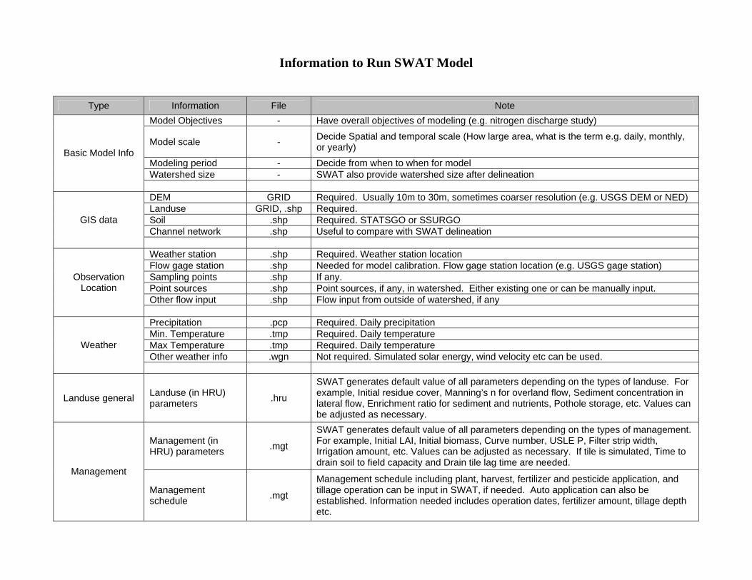
Information to Run SWAT Model
Type Information File Note
Model Objectives - Have overall objectives of modeling (e.g. nitrogen discharge study)
Model scale - Decide Spatial and temporal scale (How large area, what is the term e.g. daily, monthly, or yearly)
Modeling period - Decide from when to when for model Watershed size - SWAT also provide watershed size after delineation
Basic Model Info
DEM GRID Required. Usually 10m to 30m, sometimes coarser resolution (e.g. USGS DEM or NED) Landuse GRID, .shp Required. Soil .shp Required. STATSGO or SSURGO Channel network .shp Useful to compare with SWAT delineation
GIS data
Weather station .shp Required. Weather station location Flow gage station .shp Needed for model calibration. Flow gage station location (e.g. USGS gage station) Sampling points .shp If any. Point sources .shp Point sources, if any, in watershed. Either existing one or can be manually input. Other flow input .shp Flow input from outside of watershed, if any
Observation Location
Precipitation .pcp Required. Daily precipitation Min. Temperature .tmp Required. Daily temperature Max Temperature .tmp Required. Daily temperature Other weather info .wgn Not required. Simulated solar energy, wind velocity etc can be used.
Weather
Landuse general Landuse (in HRU) parameters
.hru
SWAT generates default value of all parameters depending on the types of landuse. For example, Initial residue cover, Manning’s n for overland flow, Sediment concentration in lateral flow, Enrichment ratio for sediment and nutrients, Pothole storage, etc. Values can be adjusted as necessary.
Management (in HRU) parameters
.mgt
SWAT generates default value of all parameters depending on the types of management. For example, Initial LAI, Initial biomass, Curve number, USLE P, Filter strip width, Irrigation amount, etc. Values can be adjusted as necessary. If tile is simulated, Time to drain soil to field capacity and Drain tile lag time are needed.
Management
Management schedule
.mgt
Management schedule including plant, harvest, fertilizer and pesticide application, and tillage operation can be input in SWAT, if needed. Auto application can also be established. Information needed includes operation dates, fertilizer amount, tillage depth etc.
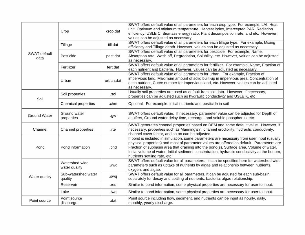
Crop crop.dat
SWAT offers default value of all parameters for each crop type. For example, LAI, Heat unit, Optimum and minimum temperature, Harvest index, Intercepted PAR, Radiation efficiency, USLE C, Biomass energy ratio, Plant decomposition rate, and etc. However, values can be adjusted as necessary.
Tillage till.dat SWAT offers default value of all parameters for each tillage type. For example, Mixing efficiency and Tillage depth. However, values can be adjusted as necessary.
Pesticide pest.dat SWAT offers default value of all parameters for pesticide. For example, Name, Absorption rate, Wash off, Degradation, Solubility, etc. However, values can be adjusted as necessary.
Fertilizer fert.dat SWAT offers default value of all parameters for fertilizer. For example, Name, Fraction of each nutrient and bacteria. However, values can be adjusted as necessary.
SWAT default data
Urban urban.dat
SWAT offers default value of all parameters for urban. For example, Fraction of impervious land, Maximum amount of solid built-up in impervious area, Concentration of each nutrient, Curve number for impervious land, etc. However, values can be adjusted as necessary.
Soil properties .sol Usually soil properties are used as default from soil data. However, if necessary, properties can be adjusted such as hydraulic conductivity and USLE K, etc
Soil Chemical properties .chm Optional. For example, initial nutrients and pesticide in soil
Ground Water Ground water properties
.gw SWAT offers default value. If necessary, parameter value can be adjusted for Depth of aquifers, Ground water delay time, recharge, and soluble phosphorus, etc
Channel Channel properties .rte SWAT generates channel properties based on DEM and some default value. However, if necessary, properties such as Manning’s n, channel erodibility, hydraulic conductivity, channel cover factor, and so on can be adjusted.
Pond Pond information .pnd
If pond is included in simulation, some parameters are necessary from user input (usually physical properties) and most of parameter values are offered as default. Parameters are Fraction of subbasin area that draining into the pond(s), Surface area, Volume of water, Initial volume of water, Initial sediment concentration, hydraulic conductivity at the bottom, nutrients settling rate, etc.
Watershed-wide water quality
.wwq SWAT offers default value for all parameters. It can be specified here for watershed wide parameters such as uptake of nutrients by algae and relationship between nutrients, oxygen, and algae.
Sub-watershed water quality
.swq SWAT offers default value for all parameters. It can be adjusted for each sub-basin separately for decay and settling of nutrients, bacteria, algae relationship.
Reservoir .res Similar to pond information, some physical properties are necessary for user to input.
Water quality
Lake .lwq Similar to pond information, some physical properties are necessary for user to input.
Point source Point source discharge
.dat Point source including flow, sediment, and nutrients can be input as hourly, daily, monthly, yearly discharge.
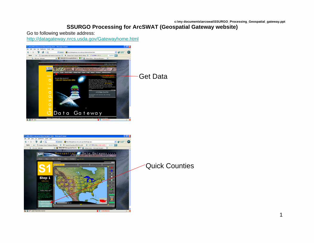
1
c:\my documents\arcswat\SSURGO_Processing_Geospatial_gateway.ppt
SSURGO Processing for ArcSWAT (Geospatial Gateway website)Go to following website address: http://datagateway.nrcs.usda.gov/Gatewayhome.html
Get Data
Quick Counties
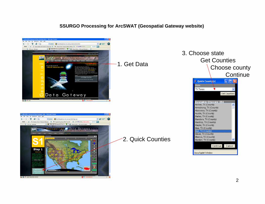
2
SSURGO Processing for ArcSWAT (Geospatial Gateway website)
1. Get Data
2. Quick Counties
3. Choose stateGet Counties
Choose countyContinue
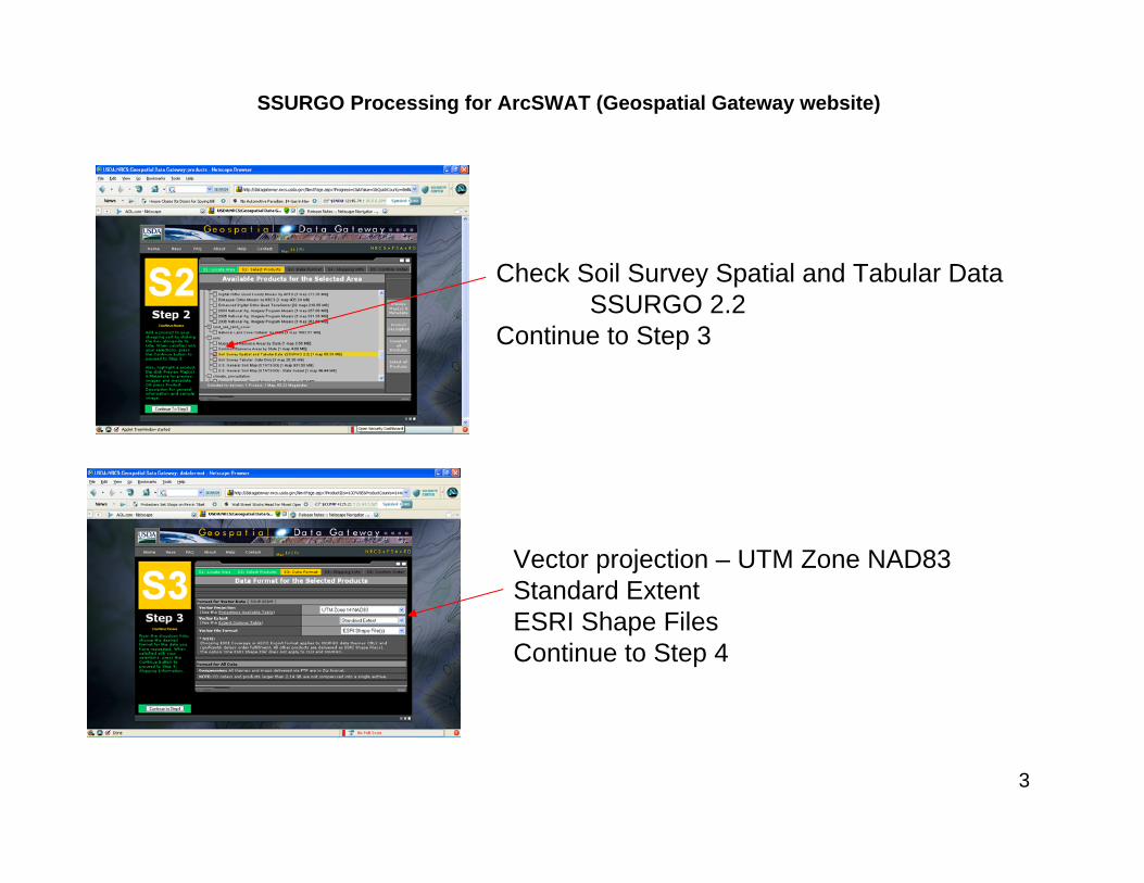
3
SSURGO Processing for ArcSWAT (Geospatial Gateway website)
Check Soil Survey Spatial and Tabular Data SSURGO 2.2
Continue to Step 3
Vector projection – UTM Zone NAD83Standard ExtentESRI Shape FilesContinue to Step 4
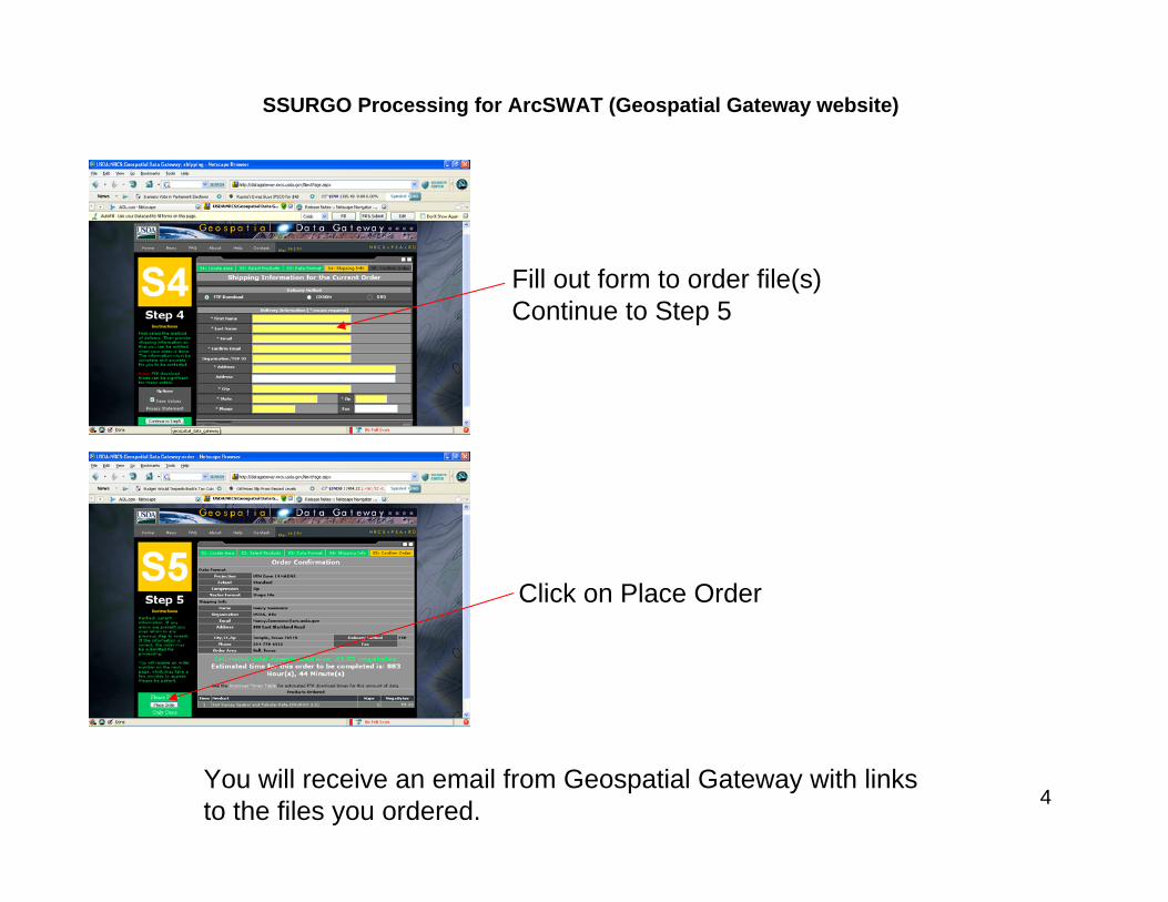
4
SSURGO Processing for ArcSWAT (Geospatial Gateway website)
Fill out form to order file(s)Continue to Step 5
Click on Place Order
You will receive an email from Geospatial Gateway with links to the files you ordered.
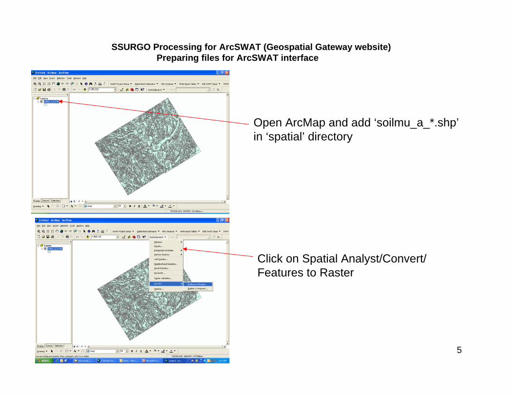
5
SSURGO Processing for ArcSWAT (Geospatial Gateway website)Preparing files for ArcSWAT interface
Open ArcMap and add ‘soilmu_a_*.shp’in ‘spatial’ directory
Click on Spatial Analyst/Convert/Features to Raster
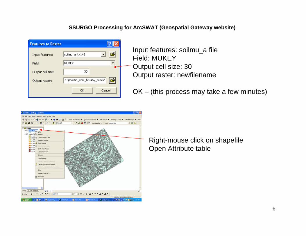
6
SSURGO Processing for ArcSWAT (Geospatial Gateway website)
Input features: soilmu_a fileField: MUKEYOutput cell size: 30Output raster: newfilename
OK – (this process may take a few minutes)
Right-mouse click on shapefileOpen Attribute table
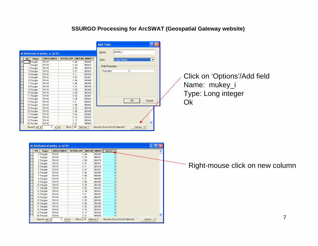
7
SSURGO Processing for ArcSWAT (Geospatial Gateway website)
Click on ‘Options’/Add fieldName: mukey_iType: Long integerOk
Right-mouse click on new column
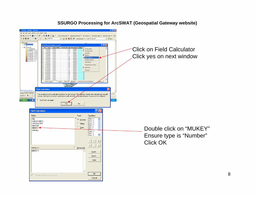
8
SSURGO Processing for ArcSWAT (Geospatial Gateway website)
Click on Field CalculatorClick yes on next window
Double click on “MUKEY”Ensure type is “Number”Click OK
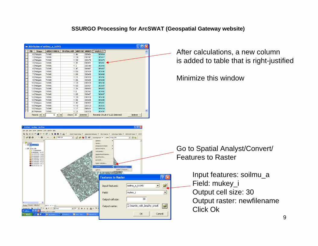
9
SSURGO Processing for ArcSWAT (Geospatial Gateway website)
After calculations, a new columnis added to table that is right-justified
Minimize this window
Go to Spatial Analyst/Convert/Features to Raster
Input features: soilmu_aField: mukey_iOutput cell size: 30Output raster: newfilenameClick Ok
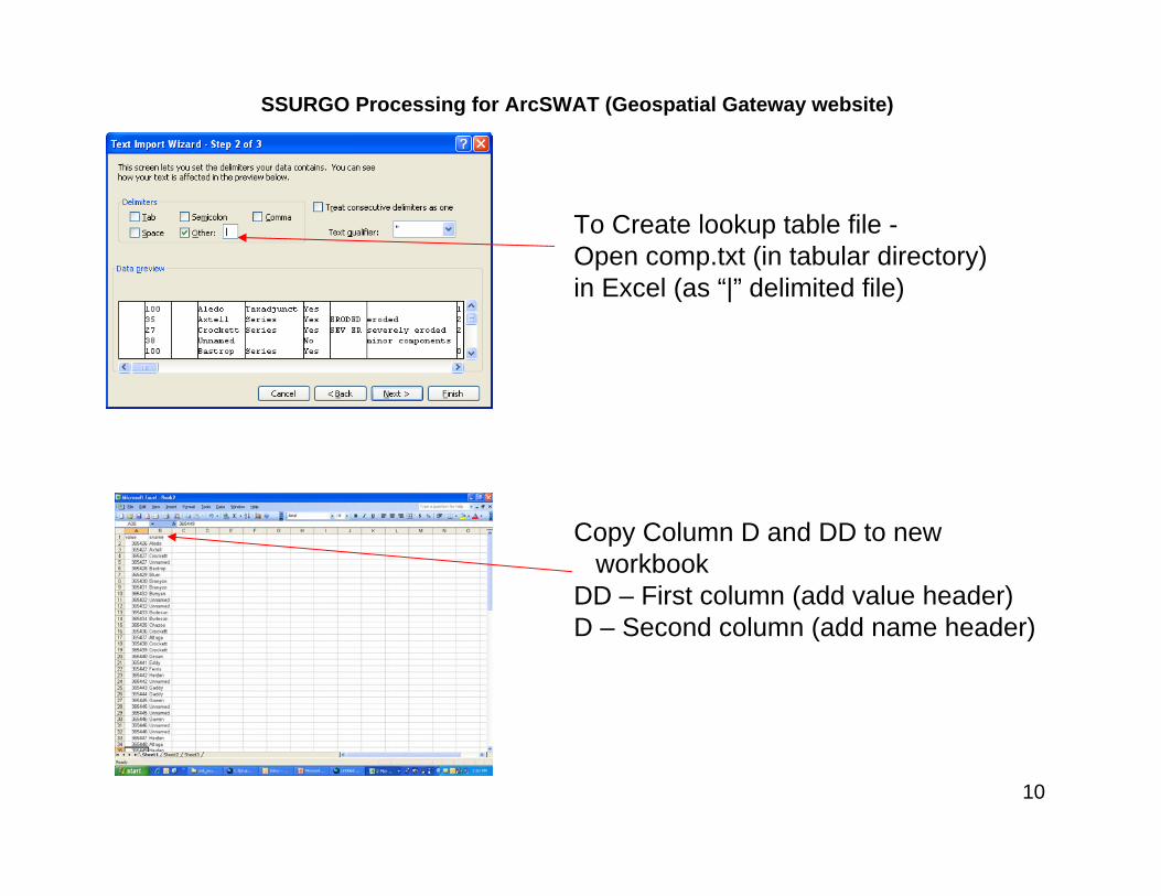
10
SSURGO Processing for ArcSWAT (Geospatial Gateway website)
To Create lookup table file -Open comp.txt (in tabular directory)in Excel (as “|” delimited file)
Copy Column D and DD to new workbook
DD – First column (add value header)D – Second column (add name header)
11
SSURGO Processing for ArcSWAT (Geospatial Gateway website)
Autofilter the ‘Unnamed’ soilsand delete
Save file as *.csv type
Browse in Windows Explorer and rename*.csv to *.txt extension.
12
If two or more counties need to be merged
Open ArcMAP/ArcToolBoxClick on Data Management Tools
General/Merge
Use the browser and add the two (or more) counties that you need merged.
Input the name of the newly merged fileClick OK.
You also need to merge the tables.
13
MERGING TWO OR MORE TABLES:Combine the comp.txt files for both counties in Excel. Delete the unnamed Soils. Add headings, save as *.csv file. Rename the .csv to .txt.(See Pages 10-11)
You must load the states SSURGO soils (get from Srini) into the SWAT2005.mdb file before using in ArcSWAT. To do this, see thefollowing document: C:\mydocuments\arcswat_instructions\arcswat_ssugo_import.ppt

Transactions of the ASABE
Vol. 50(3): 885−900 2007 American Society of Agricultural and Biological Engineers ISSN 0001−2351 885
MODEL EVALUATION GUIDELINES FOR SYSTEMATIC
QUANTIFICATION OF ACCURACY IN WATERSHED SIMULATIONS
D. N. Moriasi, J. G. Arnold, M. W. Van Liew, R. L. Bingner, R. D. Harmel, T. L. Veith
ABSTRACT. Watershed models are powerful tools for simulating the effect of watershed processes and management on soil andwater resources. However, no comprehensive guidance is available to facilitate model evaluation in terms of the accuracyof simulated data compared to measured flow and constituent values. Thus, the objectives of this research were to:(1) determine recommended model evaluation techniques (statistical and graphical), (2) review reported ranges of values andcorresponding performance ratings for the recommended statistics, and (3) establish guidelines for model evaluation basedon the review results and project-specific considerations; all of these objectives focus on simulation of streamflow andtransport of sediment and nutrients. These objectives were achieved with a thorough review of relevant literature on modelapplication and recommended model evaluation methods. Based on this analysis, we recommend that three quantitativestatistics, Nash-Sutcliffe efficiency (NSE), percent bias (PBIAS), and ratio of the root mean square error to the standarddeviation of measured data (RSR), in addition to the graphical techniques, be used in model evaluation. The following modelevaluation performance ratings were established for each recommended statistic. In general, model simulation can be judgedas satisfactory if NSE > 0.50 and RSR < 0.70, and if PBIAS � 25% for streamflow, PBIAS � 55% for sediment, and PBIAS� 70% for N and P. For PBIAS, constituent-specific performance ratings were determined based on uncertainty of measureddata. Additional considerations related to model evaluation guidelines are also discussed. These considerations include:single-event simulation, quality and quantity of measured data, model calibration procedure, evaluation time step, and projectscope and magnitude. A case study illustrating the application of the model evaluation guidelines is also provided.
Keywords. Accuracy, Model calibration and validation, Simulation, Watershed model.
omputer-based watershed models can save timeand money because of their ability to perform long-term simulation of the effects of watershed pro-cesses and management activities on water quality,
water quantity, and soil quality. These models also facilitatethe simulation of various conservation program effects andaid policy design to mitigate water and soil quality degrada-tion by determining suitable conservation programs for par-ticular watersheds and agronomic settings. In order to usemodel outputs for tasks ranging from regulation to research,models should be scientifically sound, robust, and defensible(U.S. EPA, 2002).
Submitted for review in May 2006 as manuscript number SW 6494; ap-proved for publication by the Soil & Water Division of ASABE in March2007.
The authors are Daniel N. Moriasi, ASABE Member Engineer,Hydrologist, USDA-ARS Grazinglands Research Laboratory, El Reno,Oklahoma; Jeffrey G. Arnold, Supervisory Agricultural Engineer, USDA-ARS Grassland Soil and Water Research Laboratory, Temple, Texas; Mi-chael W. Van Liew, ASABE Member Engineer, Environmental ScienceSpecialist, Water Quality Planning Bureau, Montana Department of Envi-ronmental Quality, Helena, Montana; Ronald L. Bingner, ASABE Mem-ber Engineer, Agricultural Engineer, USDA-ARS Watershed Physical Pro-cesses Research Unit, Oxford, Mississippi; R. Daren Harmel, ASABEMember Engineer, Agricultural Engineer, USDA-ARS Grassland Soil andWater Research Laboratory, Temple, Texas; and Tamie L. Veith, ASABEMember Engineer, Agricultural Engineer, USDA-ARS Pasture Systemsand Watershed Management Research Unit, University Park, Pennsylva-nia. Corresponding author: Daniel N. Moriasi, USDA-ARS GrazinglandsResearch Laboratory, 7207 W. Cheyenne St., El Reno, OK 73036-0000;phone: 405-262-5291, ext. 263; fax: 405-262-0133; e-mail: [email protected].
Sensitivity analysis is the process of determining the rateof change in model output with respect to changes in modelinputs (parameters). It is a necessary process to identify keyparameters and parameter precision required for calibration(Ma et al., 2000). Model calibration is the process of estimat-ing model parameters by comparing model predictions (out-put) for a given set of assumed conditions with observed datafor the same conditions. Model validation involves runninga model using input parameters measured or determined dur-ing the calibration process. According to Refsgaard (1997),model validation is the process of demonstrating that a givensite-specific model is capable of making “sufficiently accu-rate” simulations, although “sufficiently accurate” can varybased on project goals. According to the U.S. EPA (2002), theprocess used to accept, reject, or qualify model results shouldbe established and documented before beginning model eval-uation. Although ASCE (1993) emphasized the need to clear-ly define model evaluation criteria, no commonly acceptedguidance has been established, but specific statistics and per-formance ratings for their use have been developed and usedfor model evaluation (Donigian et al., 1983; Ramanarayananet al., 1997; Gupta et al., 1999; Motovilov et al., 1999; Salehet al., 2000; Santhi et al., 2001; Singh et al., 2004; Bracmortet al., 2006; Van Liew et al., 2007). However, these perfor-mance ratings are model and project specific. Standardizedguidelines are needed to establish a common system for judg-ing model performance and comparing various models(ASCE, 1993). Once established, these guidelines will assistmodelers in preparing and reviewing quality assurance proj-ect plans for modeling (U.S. EPA, 2002) and will increase ac-countability and public acceptance of models to support
C
886 TRANSACTIONS OF THE ASABE
scientific research and to guide policy, regulatory, and man-agement decision-making.
A number of publications have addressed model evalua-tion statistics (Willmott, 1981; ASCE, 1993; Legates andMcCabe, 1999), but they do not include recently developedstatistics (e.g., Wang and Melesse, 2005; Parker et al., 2006).More importantly, none of the previous publications provideguidance on acceptable ranges of values for each statistic.Borah and Bera (2004) present an excellent review of valuesfor various statistics used in hydrologic and nonpoint-sourcemodel applications, but more elaborate analysis is needed toaid modelers in determining performance ratings for thesestatistics.
In most watershed modeling projects, model output iscompared to corresponding measured data with the assump-tion that all error variance is contained within the predictedvalues and that observed values are error free. In discussionsof model evaluation statistics, Willmott (1981) and ASCE(1993) do recognize that measured data are not error free, butmeasurement error is not considered in their recommenda-tions perhaps because of the relative lack of data on measure-ment uncertainty. However, uncertainty estimates formeasured streamflow and water quality data have recentlybecome available (Harmel et al., 2006) and should be consid-ered when calibrating, validating, and evaluating watershedmodels because of differences in inherent uncertainty be-tween measured flow, sediment, and nutrient data.
The importance of standardized guidelines for modelevaluation is illustrated by the Conservation Effects Assess-ment Project Watershed Assessment Study (CEAP-WAS,2005). The CEAP-WAS seeks to quantify the environmentalbenefits of conservation practices supported by USDA in the2002 Farm Bill, also known as the Farm Security and RuralInvestment Act. One of the CEAP-WAS goals is to formulateguidelines for calibration, validation, and application ofmodels used in CEAP to simulate environmental effects ofconservation practices. Thus, based on the need for standard-ized model evaluation guidelines to support watershed mod-eling in CEAP-WAS and other projects, the objectives for thepresent research were to: (1) determine recommended modelevaluation techniques (statistical and graphical), (2) reviewreported ranges of values and corresponding performanceratings for the recommended statistics, and (3) establishguidelines for model evaluation based on the review resultsand project-specific considerations. In addition, a case studyillustrating the application of the model evaluation guide-lines was provided. This research focuses on watershed mod-el evaluation guidelines for streamflow, sediments, andnutrients. Throughout this article, “model evaluation” refersto the applicable steps of sensitivity analysis, calibration, val-idation, uncertainty analysis, and application.
METHODSMODEL EVALUATION TECHNIQUES
To determine recommended techniques for watershedmodel evaluation, an extensive review was conducted onpublished literature related to calibration, validation, and ap-plication of watershed models. Specifically, the informationcompiled focused on the strengths and weaknesses of eachstatistical and graphical technique and on recommendationsfor their application. The recommended model evaluation
statistics were selected based on the following factors: (1) ro-bustness in terms of applicability to various constituents,models, and climatic conditions; (2) commonly used, accept-ed, and recommended in published literature; and (3) identi-fied strengths in model evaluation. The trade-off betweenlong-term bias and residual variance was also considered, asrecommended by Boyle et al. (2000). Bias measures the aver-age tendency of the simulated constituent values to be largeror smaller than the measured data. Residual variance is thedifference between the measured and simulated values, oftenestimated by the residual mean square or root mean square er-ror (RMSE). According to Boyle et al. (2000), optimizingRMSE during model calibration may give small error vari-ance but at the expense of significant model bias. The com-pilation of recommended statistics was also constrained bythe recommendation of Legates and McCabe (1999) to in-clude at least one dimensionless statistic and one absolute er-ror index statistic with additional information such as thestandard deviation of measured data, and to include at leastone graphical technique as well.
REPORTED VALUE RANGES AND PERFORMANCE RATINGSFOR RECOMMENDED STATISTICS
Additional literature review was conducted to determinepublished ranges of values and performance ratings for rec-ommended model evaluation statistics. Reported daily andmonthly values during the calibration and validation periodsfor streamflow, sediment, and nutrients are recorded alongwith the model used for evaluation in tables A-1 through A-9in the Appendix. All the reported data were analyzed andcompiled into a summary of daily and monthly value rangesfor different constituents during calibration and validation(table 1). The summary values in table 1 include the samplesize of the reported values (n) and the minimum, maximum,and median of the values reported for streamflow, surfacerunoff, sediment, organic, mineral and total nitrogen, and or-ganic, mineral, and total phosphorus.
MODEL EVALUATION GUIDELINES
General model evaluation guidelines that consider the rec-ommended model evaluation statistics with correspondingperformance ratings and appropriate graphical analyses werethen established. A calibration procedure chart for flow, sedi-ment, and nutrients, similar to the one proposed by Santhi etal. (2001), is included to assist in application of the modelevaluation guidelines to manual model calibration. It isnoted, however, that these guidelines should be adjusted bythe modeler based on additional considerations such as:single-event simulation, quality and quantity of measureddata, model calibration procedure, evaluation time step, andproject scope and magnitude. Additionally, a brief discussionof the implications of unmet performance ratings is provided.
RESULTS AND DISCUSSIONMODEL EVALUATION TECHNIQUES
Both statistical and graphical model evaluation tech-niques were reviewed. The quantitative statistics were divid-ed into three major categories: standard regression,dimensionless, and error index. Standard regression statisticsdetermine the strength of the linear relationship between sim-ulated and measured data. Dimensionless techniques provide
887Vol. 50(3): 885−900
a relative model evaluation assessment, and error indicesquantify the deviation in the units of the data of interest (Leg-ates and McCabe, 1999). A brief discussion of numerousmodel evaluation statistics (both recommended statistics andstatistics not selected for recommendation) appears subse-quently; however, the relevant calculations are provided onlyfor the recommended statistics.
Several graphical techniques are also described briefly be-cause graphical techniques provide a visual comparison ofsimulated and measured constituent data and a first overviewof model performance (ASCE, 1993) and are essential to ap-propriate model evaluation (Legates and McCabe, 1999).Based on recommendations by ASCE (1993) and Legatesand McCabe (1999), we recommend that both graphical tech-niques and quantitative statistics be used in model evalua-tion.
MODEL EVALUATION STATISTICS (STANDARD REGRESSION)Slope and y-intercept: The slope and y-intercept of the
best-fit regression line can indicate how well simulated datamatch measured data. The slope indicates the relative rela-tionship between simulated and measured values. The y-intercept indicates the presence of a lag or lead betweenmodel predictions and measured data, or that the data sets arenot perfectly aligned. A slope of 1 and y-intercept of 0 indi-cate that the model perfectly reproduces the magnitudes ofmeasured data (Willmott, 1981). The slope and y-interceptare commonly examined under the assumption that measuredand simulated values are linearly related, which implies thatall of the error variance is contained in simulated values andthat measured data are error free (Willmott, 1981). In reality,measured data are rarely, if ever, error free. Harmel et al.(2006) showed that substantial uncertainty in reported waterquality data can result when individual errors from all proce-dural data collection categories are considered. Therefore,care needs to be taken while using regression statistics formodel evaluation.
Pearson’s correlation coefficient (r) and coefficient ofdetermination (R2): Pearson’s correlation coefficient (r)and coefficient of determination (R2) describe the degree ofcollinearity between simulated and measured data. The cor-relation coefficient, which ranges from −1 to 1, is an index ofthe degree of linear relationship between observed and simu-lated data. If r = 0, no linear relationship exists. If r = 1 or −1,a perfect positive or negative linear relationship exists. Simi-larly, R2 describes the proportion of the variance in measureddata explained by the model. R2 ranges from 0 to 1, with high-er values indicating less error variance, and typically valuesgreater than 0.5 are considered acceptable (Santhi et al.,2001, Van Liew et al., 2003). Although r and R2 have beenwidely used for model evaluation, these statistics are over-sensitive to high extreme values (outliers) and insensitive toadditive and proportional differences between model predic-tions and measured data (Legates and McCabe, 1999).
MODEL EVALUATION STATISTICS (DIMENSIONLESS)Index of agreement (d): The index of agreement (d) was
developed by Willmott (1981) as a standardized measure ofthe degree of model prediction error and varies between 0 and1. A computed value of 1 indicates a perfect agreement be-tween the measured and predicted values, and 0 indicates noagreement at all (Willmott, 1981). The index of agreement
represents the ratio between the mean square error and the“potential error” (Willmott, 1984). The author defined poten-tial error as the sum of the squared absolute values of the dis-tances from the predicted values to the mean observed valueand distances from the observed values to the mean observedvalue. The index of agreement can detect additive and pro-portional differences in the observed and simulated meansand variances; however, d is overly sensitive to extreme val-ues due to the squared differences (Legates and McCabe,1999). Legates and McCabe (1999) suggested a modified in-dex of agreement (d1) that is less sensitive to high extremevalues because errors and differences are given appropriateweighting by using the absolute value of the differenceinstead of using the squared differences. Although d1 hasbeen proposed as an improved statistic, its limited use in theliterature has not provided extensive information on valueranges.
Nash-Sutcliffe efficiency (NSE): The Nash-Sutcliffe ef-ficiency (NSE) is a normalized statistic that determines therelative magnitude of the residual variance (“noise”)compared to the measured data variance (“information”)(Nash and Sutcliffe, 1970). NSE indicates how well the plotof observed versus simulated data fits the 1:1 line. NSE iscomputed as shown in equation 1:
( )
( )
−
−−=
∑
∑
=
=n
i
meanobsi
n
i
simi
obsi
YY
YY
1
2
1
2
1NSE (1)
where Yi obs is the ith observation for the constituent beingevaluated, Yi sim is the ith simulated value for the constituentbeing evaluated, Ymean is the mean of observed data for theconstituent being evaluated, and n is the total number of ob-servations.
NSE ranges between −∞ and 1.0 (1 inclusive), with NSE =1 being the optimal value. Values between 0.0 and 1.0 aregenerally viewed as acceptable levels of performance,whereas values <0.0 indicates that the mean observed valueis a better predictor than the simulated value, which indicatesunacceptable performance.
NSE was recommended for two major reasons: (1) it isrecommended for use by ASCE (1993) and Legates andMcCabe (1999), and (2) it is very commonly used, which pro-vides extensive information on reported values. Sevat andDezetter (1991) also found NSE to be the best objective func-tion for reflecting the overall fit of a hydrograph. Legates andMcCabe (1999) suggested a modified NSE that is less sensi-tive to high extreme values due to the squared differences, butthat modified version was not selected because of its limiteduse and resulting relative lack of reported values.
Persistence model efficiency (PME): Persistence modelefficiency (PME) is a normalized model evaluation statisticthat quantifies the relative magnitude of the residual variance(“noise”) to the variance of the errors obtained by the use ofa simple persistence model (Gupta et al., 1999). PME rangesfrom 0 to 1, with PME = 1 being the optimal value. PME val-ues should be larger than 0.0 to indicate “minimally accept-able” model performance (Gupta et al., 1999). The power ofPME is derived from its comparison of model performancewith a simple persistence forecast model. According to Guptaet al. (1999), PME is capable of clearly indicating poor model
888 TRANSACTIONS OF THE ASABE
performance, but it has been used only occasionally in the lit-erature, so a range of reported values is not available.
Prediction efficiency (Pe): Prediction efficiency (Pe), asexplained by Santhi et al. (2001), is the coefficient of deter-mination (R2) calculated by regressing the rank (descending)of observed versus simulated constituent values for a giventime step. Pe determines how well the probability distribu-tions of simulated and observed data fit each other. However,it has not been used frequently enough to provide extensiveinformation on ranges of values. In addition, it may not ac-count for seasonal bias.
Performance virtue statistic (PVk): The performancevirtue statistic (PVk) is the weighted average of the Nash-Sutcliffe coefficients, deviations of volume, and error func-tions across all flow gauging stations within the watershed ofinterest (Wang and Melesse, 2005). PVk was developed to as-sess if watershed models can satisfactorily predict all aspects(profile, volume, and peak) of observed flow hydrographs forwatersheds with more than one gauging station (Wang andMelesse, 2005). PVk can range from −∞ to 1.0, with a PVkvalue of 1.0 indicating that the model exactly simulates allthree aspects of observed flow for all gauging stations withinthe watershed. A negative PVk value indicates that the aver-age of observed streamflow values is better than simulatedstreamflows (Wang and Melesse, 2005). PVk was developedfor use in snow-fed watersheds; therefore, it may be neces-sary to make adjustments to this statistic for rain-fed wa-tersheds. PVk was not selected for recommendation becauseit was developed for streamflow only. In addition, PVk wasonly recently developed; thus, extensive information on val-ue ranges is not available.
Logarithmic transformation variable (e): The logarith-mic transformation variable (e) is the logarithm of the pre-dicted/observed data ratio (E) that was developed to addressthe sensitivity of the watershed-scale pesticide model errorindex (E) to the estimated pesticide application rates (Parkeret al., 2006). The value of e is centered on zero, is symmetri-cal in under- or overprediction, and is approximately normal-ly distributed (Parker et al., 2006). If the simulated andmeasured data are in complete agreement, then e = 0 and E =1.0. Values of e < 0 are indicative of underprediction; values> 0 are indicative of overprediction. Although e has great po-tential as an improved statistical technique for assessingmodel accuracy, it was not selected because of its recent de-velopment and limited testing and application.
MODEL EVALUATION STATISTICS (ERROR INDEX)MAE, MSE, and RMSE: Several error indices are com-
monly used in model evaluation. These include mean abso-lute error (MAE), mean square error (MSE), and root meansquare error (RMSE). These indices are valuable becausethey indicate error in the units (or squared units) of the con-stituent of interest, which aids in analysis of the results.RMSE, MAE, and MSE values of 0 indicate a perfect fit.Singh et al. (2004) state that RMSE and MAE values less thanhalf the standard deviation of the measured data may be con-sidered low and that either is appropriate for model evalua-tion. A standardized version of the RMSE was selected forrecommendation and is described later in this section.
Percent bias (PBIAS): Percent bias (PBIAS) measuresthe average tendency of the simulated data to be larger orsmaller than their observed counterparts (Gupta et al., 1999).
The optimal value of PBIAS is 0.0, with low-magnitude val-ues indicating accurate model simulation. Positive values in-dicate model underestimation bias, and negative valuesindicate model overestimation bias (Gupta et al., 1999).PBIAS is calculated with equation 2:
( )
( )
−
=∑
∑
=
=n
i
obsi
n
i
simi
obsi
Y
YY
1
1
)100(*
PBIAS (2)
where PBIAS is the deviation of data being evaluated, ex-pressed as a percentage.
Percent streamflow volume error (PVE; Singh et al.,2004), prediction error (PE; Fernandez et al., 2005), and per-cent deviation of streamflow volume (Dv) are calculated ina similar manner as PBIAS. The deviation term (Dv) is usedto evaluate the accumulation of differences in streamflowvolume between simulated and measured data for a particularperiod of analysis.
PBIAS was selected for recommendation for several rea-sons: (1) Dv was recommended by ASCE (1993), (2) Dv iscommonly used to quantify water balance errors and its usecan easily be extended to load errors, and (3) PBIAS has theability to clearly indicate poor model performance (Gupta etal., 1999). PBIAS values for streamflow tend to vary more,among different autocalibration methods, during dry yearsthan during wet years (Gupta et al., 1999). This fact shouldbe considered when attempting to do a split-sample evalua-tion, one for calibration and one for validation.
RMSE-observations standard deviation ratio (RSR):RMSE is one of the commonly used error index statistics(Chu and Shirmohammadi, 2004; Singh et al., 2004;Vasquez-Amábile and Engel, 2005). Although it is common-ly accepted that the lower the RMSE the better the model per-formance, only Singh et al. (2004) have published a guidelineto qualify what is considered a low RMSE based on the ob-servations standard deviation. Based on the recommendationby Singh et al. (2004), a model evaluation statistic, named theRMSE-observations standard deviation ratio (RSR), was de-veloped. RSR standardizes RMSE using the observationsstandard deviation, and it combines both an error index andthe additional information recommended by Legates andMcCabe (1999). RSR is calculated as the ratio of the RMSEand standard deviation of measured data, as shown in equa-tion 3:
( )
( )
−
−
==
∑
∑
=
=
n
i
meanobsi
n
i
simi
obsi
obs
YY
YY
1
2
1
2
STDEVRMSE
RSR (3)
RSR incorporates the benefits of error index statistics andincludes a scaling/normalization factor, so that the resultingstatistic and reported values can apply to various constitu-ents. RSR varies from the optimal value of 0, which indicateszero RMSE or residual variation and therefore perfect modelsimulation, to a large positive value. The lower RSR, the low-er the RMSE, and the better the model simulation perfor-mance.
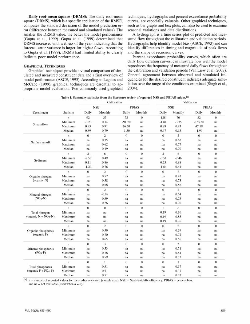
889Vol. 50(3): 885−900
Daily root-mean square (DRMS): The daily root-meansquare (DRMS), which is a specific application of the RMSE,computes the standard deviation of the model prediction er-ror (difference between measured and simulated values). Thesmaller the DRMS value, the better the model performance(Gupta et al., 1999). Gupta et al. (1999) determined thatDRMS increased with wetness of the year, indicating that theforecast error variance is larger for higher flows. Accordingto Gupta et al. (1999), DRMS had limited ability to clearlyindicate poor model performance.
GRAPHICAL TECHNIQUES
Graphical techniques provide a visual comparison of sim-ulated and measured constituent data and a first overview ofmodel performance (ASCE, 1993). According to Legates andMcCabe (1999), graphical techniques are essential to ap-propriate model evaluation. Two commonly used graphical
techniques, hydrographs and percent exceedance probabilitycurves, are especially valuable. Other graphical techniques,such as bar graphs and box plots, can also be used to examineseasonal variations and data distributions.
A hydrograph is a time series plot of predicted and mea-sured flow throughout the calibration and validation periods.Hydrographs help identify model bias (ASCE, 1993) and canidentify differences in timing and magnitude of peak flowsand the shape of recession curves.
Percent exceedance probability curves, which often aredaily flow duration curves, can illustrate how well the modelreproduces the frequency of measured daily flows throughoutthe calibration and validation periods (Van Liew et al., 2007).General agreement between observed and simulated fre-quencies for the desired constituent indicates adequate simu-lation over the range of the conditions examined (Singh et al.,2004).
Table 1. Summary statistics from the literature review of reported NSE and PBIAS values.[a]
Calibration Validation
NSE PBIAS NSE PBIAS
Constituent Statistic Daily Monthly Daily Monthly Daily Monthly Daily Monthly
Streamflow
n 92 33 72 0 128 70 82 0Minimum -0.23 0.14 -91.70 na -1.81 -3.35 -155.60 naMaximum 0.95 0.91 26.50 na 0.89 0.93 47.18 na
Median 0.89 0.79 -1.30 na 0.67 0.63 -1.90 na
Surface runoff
n 0 2 0 0 0 2 0 0Minimum na 0.35 na na na 0.63 na naMaximum na 0.62 na na na 0.77 na na
Median na 0.49 na na na 0.70 na na
Sediment
n 2 6 0 0 2 6 0 0Minimum -2.50 0.49 na na -3.51 -2.46 na naMaximum 0.11 0.86 na na 0.23 0.88 na na
Median -1.20 0.76 na na -1.64 0.64 na na
Organic nitrogen(organic N)
n 0 2 0 0 0 2 0 0Minimum na 0.57 na na na 0.43 na naMaximum na 0.58 na na na 0.73 na na
Median na 0.58 na na na 0.58 na na
Mineral nitrogen(NO3-N)
n 0 2 0 0 0 2 0 0Minimum na -0.08 na na na 0.64 na naMaximum na 0.59 na na na 0.75 na na
Median na 0.26 na na na 0.70 na na
Total nitrogen(organic N + NO3-N)
n 0 0 0 0 1 6 0 0Minimum na na na na 0.19 0.10 na naMaximum na na na na 0.19 0.85 na na
Median na na na na 0.19 0.76 na na
Organic phosphorus(organic P)
n 0 2 0 0 0 2 0 0Minimum na 0.59 na na na 0.39 na naMaximum na 0.70 na na na 0.72 na na
Median na 0.65 na na na 0.56 na na
Mineral phosphorus(PO4-P)
n 0 3 0 0 0 3 0 0Minimum na 0.53 na na na 0.51 na naMaximum na 0.78 na na na 0.81 na na
Median na 0.59 na na na 0.53 na na
Total phosphorus(organic P + PO4-P)
n 0 1 0 0 0 1 0 0Minimum na 0.51 na na na 0.37 na naMaximum na 0.51 na na na 0.37 na na
Median na 0.51 na na na 0.37 na na[a] n = number of reported values for the studies reviewed (sample size), NSE = Nash-Sutcliffe efficiency, PBIAS = percent bias,
and na = not available (used when n = 0).
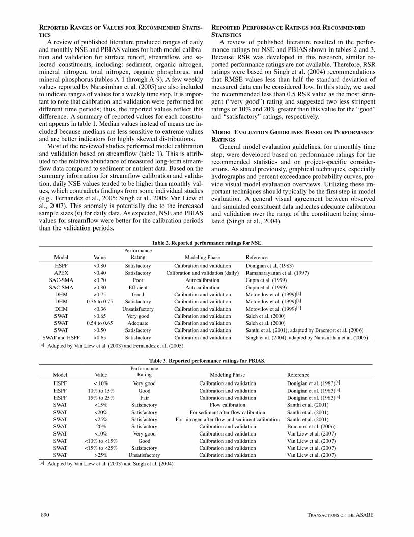
890 TRANSACTIONS OF THE ASABE
REPORTED RANGES OF VALUES FOR RECOMMENDED STATIS-TICS
A review of published literature produced ranges of dailyand monthly NSE and PBIAS values for both model calibra-tion and validation for surface runoff, streamflow, and se-lected constituents, including: sediment, organic nitrogen,mineral nitrogen, total nitrogen, organic phosphorus, andmineral phosphorus (tables A-1 through A-9). A few weeklyvalues reported by Narasimhan et al. (2005) are also includedto indicate ranges of values for a weekly time step. It is impor-tant to note that calibration and validation were performed fordifferent time periods; thus, the reported values reflect thisdifference. A summary of reported values for each constitu-ent appears in table 1. Median values instead of means are in-cluded because medians are less sensitive to extreme valuesand are better indicators for highly skewed distributions.
Most of the reviewed studies performed model calibrationand validation based on streamflow (table 1). This is attrib-uted to the relative abundance of measured long-term stream-flow data compared to sediment or nutrient data. Based on thesummary information for streamflow calibration and valida-tion, daily NSE values tended to be higher than monthly val-ues, which contradicts findings from some individual studies(e.g., Fernandez et al., 2005; Singh et al., 2005; Van Liew etal., 2007). This anomaly is potentially due to the increasedsample sizes (n) for daily data. As expected, NSE and PBIASvalues for streamflow were better for the calibration periodsthan the validation periods.
REPORTED PERFORMANCE RATINGS FOR RECOMMENDEDSTATISTICS
A review of published literature resulted in the perfor-mance ratings for NSE and PBIAS shown in tables 2 and 3.Because RSR was developed in this research, similar re-ported performance ratings are not available. Therefore, RSRratings were based on Singh et al. (2004) recommendationsthat RMSE values less than half the standard deviation ofmeasured data can be considered low. In this study, we usedthe recommended less than 0.5 RSR value as the most strin-gent (“very good”) rating and suggested two less stringentratings of 10% and 20% greater than this value for the “good”and “satisfactory” ratings, respectively.
MODEL EVALUATION GUIDELINES BASED ON PERFORMANCE
RATINGSGeneral model evaluation guidelines, for a monthly time
step, were developed based on performance ratings for therecommended statistics and on project-specific consider-ations. As stated previously, graphical techniques, especiallyhydrographs and percent exceedance probability curves, pro-vide visual model evaluation overviews. Utilizing these im-portant techniques should typically be the first step in modelevaluation. A general visual agreement between observedand simulated constituent data indicates adequate calibrationand validation over the range of the constituent being simu-lated (Singh et al., 2004).
Table 2. Reported performance ratings for NSE.
Model ValuePerformance
Rating Modeling Phase Reference
HSPF >0.80 Satisfactory Calibration and validation Donigian et al. (1983)APEX >0.40 Satisfactory Calibration and validation (daily) Ramanarayanan et al. (1997)
SAC-SMA <0.70 Poor Autocalibration Gupta et al. (1999)SAC-SMA >0.80 Efficient Autocalibration Gupta et al. (1999)
DHM >0.75 Good Calibration and validation Motovilov et al. (1999)[a]
DHM 0.36 to 0.75 Satisfactory Calibration and validation Motovilov et al. (1999)[a]
DHM <0.36 Unsatisfactory Calibration and validation Motovilov et al. (1999)[a]
SWAT >0.65 Very good Calibration and validation Saleh et al. (2000)SWAT 0.54 to 0.65 Adequate Calibration and validation Saleh et al. (2000)SWAT >0.50 Satisfactory Calibration and validation Santhi et al. (2001); adapted by Bracmort et al. (2006)
SWAT and HSPF >0.65 Satisfactory Calibration and validation Singh et al. (2004); adapted by Narasimhan et al. (2005)[a] Adapted by Van Liew et al. (2003) and Fernandez et al. (2005).
Table 3. Reported performance ratings for PBIAS.
Model ValuePerformance
Rating Modeling Phase Reference
HSPF < 10% Very good Calibration and validation Donigian et al. (1983)[a]
HSPF 10% to 15% Good Calibration and validation Donigian et al. (1983)[a]
HSPF 15% to 25% Fair Calibration and validation Donigian et al. (1983)[a]
SWAT <15% Satisfactory Flow calibration Santhi et al. (2001)SWAT <20% Satisfactory For sediment after flow calibration Santhi et al. (2001)SWAT <25% Satisfactory For nitrogen after flow and sediment calibration Santhi et al. (2001)SWAT 20% Satisfactory Calibration and validation Bracmort et al. (2006)SWAT <10% Very good Calibration and validation Van Liew et al. (2007)SWAT <10% to <15% Good Calibration and validation Van Liew et al. (2007)SWAT <15% to <25% Satisfactory Calibration and validation Van Liew et al. (2007)SWAT >25% Unsatisfactory Calibration and validation Van Liew et al. (2007)
[a] Adapted by Van Liew et al. (2003) and Singh et al. (2004).
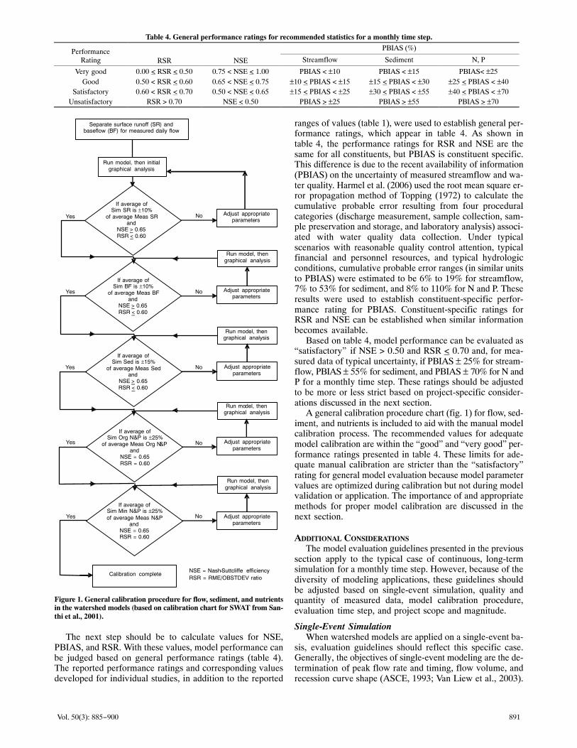
891Vol. 50(3): 885−900
Table 4. General performance ratings for recommended statistics for a monthly time step.
PerformanceRating RSR NSE
PBIAS (%)
Streamflow Sediment N, P
Very good 0.00 < RSR < 0.50 0.75 < NSE < 1.00 PBIAS < ±10 PBIAS < ±15 PBIAS< ±25Good 0.50 < RSR < 0.60 0.65 < NSE < 0.75 ±10 < PBIAS < ±15 ±15 < PBIAS < ±30 ±25 < PBIAS < ±40
Satisfactory 0.60 < RSR < 0.70 0.50 < NSE < 0.65 ±15 < PBIAS < ±25 ±30 < PBIAS < ±55 ±40 < PBIAS < ±70Unsatisfactory RSR > 0.70 NSE < 0.50 PBIAS > ±25 PBIAS > ±55 PBIAS > ±70
Separate surface runoff (SR) andbaseflow (BF) for measured daily flow
NSE = Nash−Suttcliffe efficiencyRSR = RME/OBSTDEV ratio
Calibration complete
Yes No
NoYes
NoYes
Yes No
NoYes
Run model, then initialgraphical analysis
Adjust appropriateparameters
Run model, thengraphical analysis
Run model, thengraphical analysis
Run model, thengraphical analysis
Run model, thengraphical analysis
Adjust appropriateparameters
Adjust appropriateparameters
Adjust appropriateparameters
Adjust appropriateparameters
If average ofSim SR is ±10%
of average Meas SRand
NSE > 0.65RSR < 0.60
If average ofSim BF is ±10%
of average Meas BFand
NSE > 0.65RSR < 0.60
If average ofSim Sed is ±15%
of average Meas Sedand
NSE > 0.65RSR < 0.60
If average ofSim Org N&P is ±25%
of average Meas Org N&Pand
NSE = 0.65RSR = 0.60
If average ofSim Min N&P is ±25%of average Meas N&P
andNSE = 0.65RSR = 0.60
Figure 1. General calibration procedure for flow, sediment, and nutrientsin the watershed models (based on calibration chart for SWAT from San-thi et al., 2001).
The next step should be to calculate values for NSE,PBIAS, and RSR. With these values, model performance canbe judged based on general performance ratings (table 4).The reported performance ratings and corresponding valuesdeveloped for individual studies, in addition to the reported
ranges of values (table 1), were used to establish general per-formance ratings, which appear in table 4. As shown intable 4, the performance ratings for RSR and NSE are thesame for all constituents, but PBIAS is constituent specific.This difference is due to the recent availability of information(PBIAS) on the uncertainty of measured streamflow and wa-ter quality. Harmel et al. (2006) used the root mean square er-ror propagation method of Topping (1972) to calculate thecumulative probable error resulting from four proceduralcategories (discharge measurement, sample collection, sam-ple preservation and storage, and laboratory analysis) associ-ated with water quality data collection. Under typicalscenarios with reasonable quality control attention, typicalfinancial and personnel resources, and typical hydrologicconditions, cumulative probable error ranges (in similar unitsto PBIAS) were estimated to be 6% to 19% for streamflow,7% to 53% for sediment, and 8% to 110% for N and P. Theseresults were used to establish constituent-specific perfor-mance rating for PBIAS. Constituent-specific ratings forRSR and NSE can be established when similar informationbecomes available.
Based on table 4, model performance can be evaluated as“satisfactory” if NSE > 0.50 and RSR < 0.70 and, for mea-sured data of typical uncertainty, if PBIAS ± 25% for stream-flow, PBIAS ± 55% for sediment, and PBIAS ± 70% for N andP for a monthly time step. These ratings should be adjustedto be more or less strict based on project-specific consider-ations discussed in the next section.
A general calibration procedure chart (fig. 1) for flow, sed-iment, and nutrients is included to aid with the manual modelcalibration process. The recommended values for adequatemodel calibration are within the “good” and “very good” per-formance ratings presented in table 4. These limits for ade-quate manual calibration are stricter than the “satisfactory”rating for general model evaluation because model parametervalues are optimized during calibration but not during modelvalidation or application. The importance of and appropriatemethods for proper model calibration are discussed in thenext section.
ADDITIONAL CONSIDERATIONS
The model evaluation guidelines presented in the previoussection apply to the typical case of continuous, long-termsimulation for a monthly time step. However, because of thediversity of modeling applications, these guidelines shouldbe adjusted based on single-event simulation, quality andquantity of measured data, model calibration procedure,evaluation time step, and project scope and magnitude.
Single-Event SimulationWhen watershed models are applied on a single-event ba-
sis, evaluation guidelines should reflect this specific case.Generally, the objectives of single-event modeling are the de-termination of peak flow rate and timing, flow volume, andrecession curve shape (ASCE, 1993; Van Liew et al., 2003).
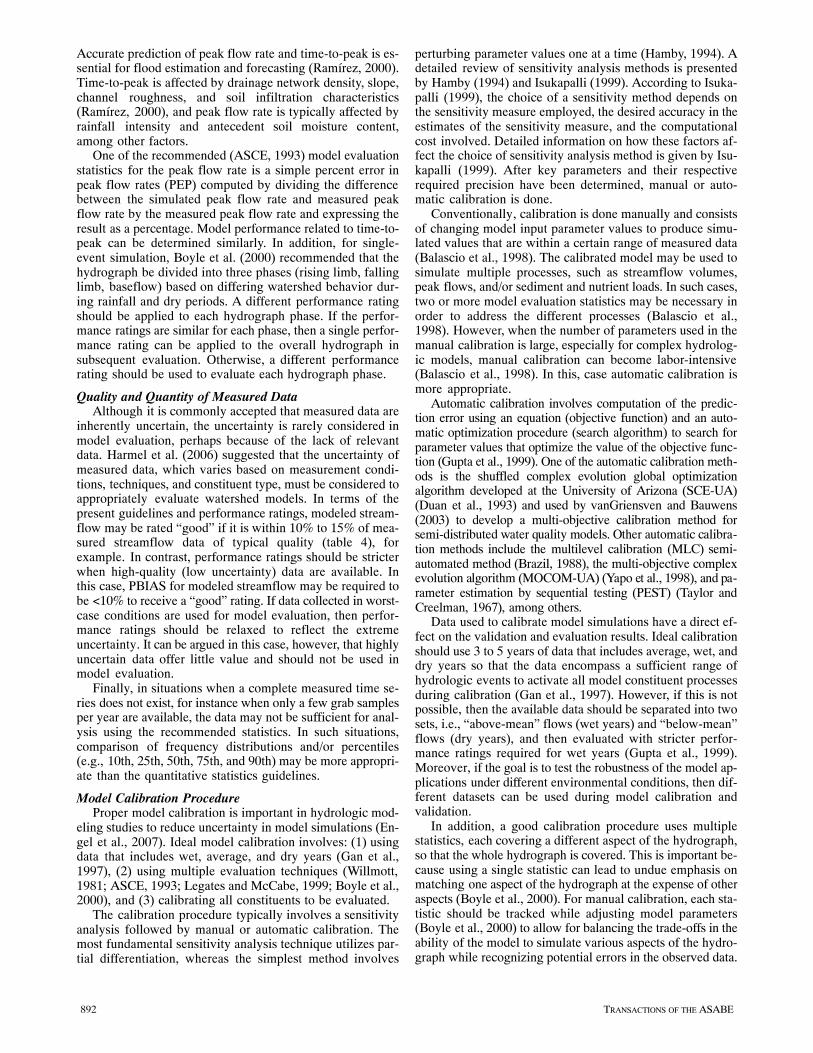
892 TRANSACTIONS OF THE ASABE
Accurate prediction of peak flow rate and time-to-peak is es-sential for flood estimation and forecasting (Ramírez, 2000).Time-to-peak is affected by drainage network density, slope,channel roughness, and soil infiltration characteristics(Ramírez, 2000), and peak flow rate is typically affected byrainfall intensity and antecedent soil moisture content,among other factors.
One of the recommended (ASCE, 1993) model evaluationstatistics for the peak flow rate is a simple percent error inpeak flow rates (PEP) computed by dividing the differencebetween the simulated peak flow rate and measured peakflow rate by the measured peak flow rate and expressing theresult as a percentage. Model performance related to time-to-peak can be determined similarly. In addition, for single-event simulation, Boyle et al. (2000) recommended that thehydrograph be divided into three phases (rising limb, fallinglimb, baseflow) based on differing watershed behavior dur-ing rainfall and dry periods. A different performance ratingshould be applied to each hydrograph phase. If the perfor-mance ratings are similar for each phase, then a single perfor-mance rating can be applied to the overall hydrograph insubsequent evaluation. Otherwise, a different performancerating should be used to evaluate each hydrograph phase.
Quality and Quantity of Measured DataAlthough it is commonly accepted that measured data are
inherently uncertain, the uncertainty is rarely considered inmodel evaluation, perhaps because of the lack of relevantdata. Harmel et al. (2006) suggested that the uncertainty ofmeasured data, which varies based on measurement condi-tions, techniques, and constituent type, must be considered toappropriately evaluate watershed models. In terms of thepresent guidelines and performance ratings, modeled stream-flow may be rated “good” if it is within 10% to 15% of mea-sured streamflow data of typical quality (table 4), forexample. In contrast, performance ratings should be stricterwhen high-quality (low uncertainty) data are available. Inthis case, PBIAS for modeled streamflow may be required tobe <10% to receive a “good” rating. If data collected in worst-case conditions are used for model evaluation, then perfor-mance ratings should be relaxed to reflect the extremeuncertainty. It can be argued in this case, however, that highlyuncertain data offer little value and should not be used inmodel evaluation.
Finally, in situations when a complete measured time se-ries does not exist, for instance when only a few grab samplesper year are available, the data may not be sufficient for anal-ysis using the recommended statistics. In such situations,comparison of frequency distributions and/or percentiles(e.g., 10th, 25th, 50th, 75th, and 90th) may be more appropri-ate than the quantitative statistics guidelines.
Model Calibration ProcedureProper model calibration is important in hydrologic mod-
eling studies to reduce uncertainty in model simulations (En-gel et al., 2007). Ideal model calibration involves: (1) usingdata that includes wet, average, and dry years (Gan et al.,1997), (2) using multiple evaluation techniques (Willmott,1981; ASCE, 1993; Legates and McCabe, 1999; Boyle et al.,2000), and (3) calibrating all constituents to be evaluated.
The calibration procedure typically involves a sensitivityanalysis followed by manual or automatic calibration. Themost fundamental sensitivity analysis technique utilizes par-tial differentiation, whereas the simplest method involves
perturbing parameter values one at a time (Hamby, 1994). Adetailed review of sensitivity analysis methods is presentedby Hamby (1994) and Isukapalli (1999). According to Isuka-palli (1999), the choice of a sensitivity method depends onthe sensitivity measure employed, the desired accuracy in theestimates of the sensitivity measure, and the computationalcost involved. Detailed information on how these factors af-fect the choice of sensitivity analysis method is given by Isu-kapalli (1999). After key parameters and their respectiverequired precision have been determined, manual or auto-matic calibration is done.
Conventionally, calibration is done manually and consistsof changing model input parameter values to produce simu-lated values that are within a certain range of measured data(Balascio et al., 1998). The calibrated model may be used tosimulate multiple processes, such as streamflow volumes,peak flows, and/or sediment and nutrient loads. In such cases,two or more model evaluation statistics may be necessary inorder to address the different processes (Balascio et al.,1998). However, when the number of parameters used in themanual calibration is large, especially for complex hydrolog-ic models, manual calibration can become labor-intensive(Balascio et al., 1998). In this, case automatic calibration ismore appropriate.
Automatic calibration involves computation of the predic-tion error using an equation (objective function) and an auto-matic optimization procedure (search algorithm) to search forparameter values that optimize the value of the objective func-tion (Gupta et al., 1999). One of the automatic calibration meth-ods is the shuffled complex evolution global optimizationalgorithm developed at the University of Arizona (SCE-UA)(Duan et al., 1993) and used by vanGriensven and Bauwens(2003) to develop a multi-objective calibration method forsemi-distributed water quality models. Other automatic calibra-tion methods include the multilevel calibration (MLC) semi-automated method (Brazil, 1988), the multi-objective complexevolution algorithm (MOCOM-UA) (Yapo et al., 1998), and pa-rameter estimation by sequential testing (PEST) (Taylor andCreelman, 1967), among others.
Data used to calibrate model simulations have a direct ef-fect on the validation and evaluation results. Ideal calibrationshould use 3 to 5 years of data that includes average, wet, anddry years so that the data encompass a sufficient range ofhydrologic events to activate all model constituent processesduring calibration (Gan et al., 1997). However, if this is notpossible, then the available data should be separated into twosets, i.e., “above-mean” flows (wet years) and “below-mean”flows (dry years), and then evaluated with stricter perfor-mance ratings required for wet years (Gupta et al., 1999).Moreover, if the goal is to test the robustness of the model ap-plications under different environmental conditions, then dif-ferent datasets can be used during model calibration andvalidation.
In addition, a good calibration procedure uses multiplestatistics, each covering a different aspect of the hydrograph,so that the whole hydrograph is covered. This is important be-cause using a single statistic can lead to undue emphasis onmatching one aspect of the hydrograph at the expense of otheraspects (Boyle et al., 2000). For manual calibration, each sta-tistic should be tracked while adjusting model parameters(Boyle et al., 2000) to allow for balancing the trade-offs in theability of the model to simulate various aspects of the hydro-graph while recognizing potential errors in the observed data.
893Vol. 50(3): 885−900
Finally, ideal model calibration considers water balance(peak flow, baseflow) and sediment and nutrient transport be-cause calibrating one constituent will not ensure that otherconstituents are adequately simulated during validation.Even though a complete set of hydrologic and water qualitydata are rarely available, all available data should be consid-ered. To calibrate water balance, it is recommended to sepa-rate baseflow and surface flow (surface runoff) from the totalstreamflow for both the measured and simulated data usinga baseflow filter program. The baseflow filter developed byArnold et al. (1995) and modified by Arnold and Allen (1999)is available at www.brc.tamus.edu/swat/soft_baseflow .html.Baseflow and recharge data from this procedure have showngood correlation with those produced by SWAT (Arnold etal., 2000). With estimated baseflow data, the baseflow ratiocan be computed for measured and simulated data by divid-ing baseflow estimates by the total measured or simulatedstreamflow. The calibration and validation process can beconsidered satisfactory if the estimated baseflow ratio forsimulated flow is within 20% of the measured flow baseflowratio (Bracmort et al., 2006). Because plant growth and bio-mass production can have an effect on the water balance, rea-sonable local/regional plant growth days and biomassproduction may need to be verified during model calibration.Annual local/regional evapotranspiration (ET) may alsoneed to be verified or compared with measured estimates dur-ing model calibration.
Stricter performance ratings should generally be requiredduring model calibration than during validation. This differ-ence is recommended because parameter values are opti-mized during model calibration, but parameters are notadjusted in validation, which is possibly conducted under dif-ferent conditions than those occurring during calibration. Al-though the importance of model calibration is wellestablished, performance ratings can be relaxed if impropercalibration procedures are employed.
It is necessary to note that although proper model calibra-tion is important in reducing error in model output, experi-ence has shown that model simulation results may containsubstantial errors. Therefore, rather than provide a point esti-mate of a given quantity of model output, it may be preferableto provide an interval estimate with an associated probabilitythat the value of the quantity will be contained by the interval(Haan et al., 1998). In other words, uncertainty analysis needsto be included in model evaluations. Uncertainty analysis isdefined as the process of quantifying the level of confidencein a given model simulation output based on: (1) the qualityand amount of measured data available, (2) the absence ofmeasured data due to the lack of monitoring in certain loca-tions, (3) the lack of knowledge about some physical pro-cesses and operational procedures, (4) the approximatenature of the mathematical equations used to simulate pro-cesses, and (5) the quality of the model sensitivity analysisand calibration. Detailed model uncertainty analysis is be-yond the scope of this research, but more model output uncer-tainty information can be obtained from published literature.
Evaluation Time StepMost of the literature reviewed used daily and/or monthly
time steps (Saleh et al., 2000; Santhi et al., 2001; Yuan et al.,2001; Sands et al., 2003; Van Liew et al., 2003; Chu and Shir-mohammadi, 2004; Saleh and Du, 2004; Singh et al., 2004;Bracmort et al., 2006; Singh et al., 2005; Van Liew et al.,
2007), although a few used annual time steps (Gupta et al.,1999; Shirmohammadi et al., 2001; Reyes et al., 2004), andone used weekly time steps (Narasimhan et al., 2005). There-fore, the time steps considered in this article are the daily andmonthly. Typically, model simulations are poorer for shortertime steps than for longer time steps (e.g., daily versusmonthly or yearly) (Engel et al., 2007). For example, Yuanet al. (2001) reported an R2 value of 0.5 for event comparisonof predicted and observed sediment yields, and an R2 valueof 0.7 for monthly comparison. The NSE values were 0.395and 0.656 for daily and monthly, respectively, forDRAINMOD-DUFLOW calibration, and 0.363 and 0.664for daily and monthly, respectively, for DRAINMOD-W cal-ibration (Fernandez et al., 2005). Similarly, the NSE valueswere 0.536 and 0.870 for daily and monthly, respectively, forDRAINMOD-DUFLOW validation, and 0.457 and 0.857 fordaily and monthly, respectively, for DRAINMOD-W valida-tion (Fernandez et al., 2005). Additional research work thatsupports the described findings includes that of Santhi et al.(2001), Van Liew et al. (2003), and Van Liew et al. (2007) us-ing SWAT. The performance ratings presented in table 4 forRSR and NSE statistics are for a monthly time step; therefore,they need to be modified appropriately. Generally, as theevaluation time step increases, a stricter performance ratingis warranted.
Project Scope and MagnitudeThe scope and magnitude of the modeling project also af-
fects model evaluation guidelines. The intended use of themodel is an indication of the seriousness of the potential con-sequences or impacts of decisions made based on model re-sults (U.S. EPA, 2002). For instance, stricter performancerating requirements need to be set for projects that involvepotentially large consequences, such as congressional testi-mony, development of new laws and regulations, or the sup-port of litigation. More modest performance ratings would beacceptable for technology assessment or “proof of principle,”where no litigation or regulatory action is expected. Evenlower performance ratings will suffice if the model is used forbasic exploratory research requiring extremely fast turn-around or high flexibility.
Finally, according to the U.S. EPA (2002), if model simu-lation does not yield acceptable results based on predefinedperformance ratings, this may indicate that: (1) conditions inthe calibration period were significantly different from thosein the validation period, (2) the model was inadequately orimproperly calibrated, (3) measured data were inaccurate,(4) more detailed inputs are required, and/or (5) the model isunable to adequately represent the watershed processes of in-terest.
A CASE STUDYPROJECT DESCRIPTION
As a component of the CEAP-WAS, the Soil and WaterAssessment Tool (SWAT2005; Arnold et al., 1998) was ap-plied to the Leon River watershed in Texas. The watersheddrains into Lake Belton, which lies within Bell and Coryellcounties and provides flood control, water supply, and publicrecreation. The lake has a surface area of approximately12,300 acres with a maximum depth of 124 feet. The totalconservation storage is 372,700 ac-ft. The Lake Belton wa-tershed (Leon River) covers approximately 2.3 million acres
894 TRANSACTIONS OF THE ASABE
within five counties in central Texas. The majority of the landuse in the watershed is pasture, hay, and brushy rangeland(63%). Cropland comprises about 10% of the watershed area.The northwestern (upper) half of the watershed contains nu-merous animal feeding operations, mainly dairies. Currently,there are approximately 60 permitted dairies and 40 smallerdairies (not requiring permits), with approximately 70,000total cows. The main goal of the study is to use SWAT2005to predict the impact of land management on the watershedover long periods of time, with special focus on waste man-agement practices.
To accomplish this goal, SWAT2005, with its many inputparameters that describe physical, chemical, and biologicalprocesses, required calibration for application in the studywatershed. Proper model calibration is important in hydro-logic modeling studies to reduce uncertainty in model predic-tions. For a general description of proper model calibration
procedures, refer to the previous discussion in the AdditionalConsiderations section.
MODEL EVALUATION RESULTS BASED ON THE DEVELOPEDGUIDELINES
When these model performance ratings were applied tothe SWAT2005 modeling in the Leon River (Lake Belton)watershed, the following results were obtained (figs. 2 and 3,table 5). Graphical results during calibration (fig. 2) and val-idation (fig. 3) indicated adequate calibration and validationover the range of streamflow, although the calibration resultsshowed a better match than the validation results. NSE valuesfor the monthly streamflow calibration and validation rangedfrom 0.66 to 1.00. According to the model evaluation guide-lines, SWAT2005 simulated the streamflow trends well tovery well, as shown by the statistical results, which are inagreement with the graphical results. The RSR values ranged
Figure 2. Monthly discharge (CMS) calibration for the Leon River sub-basin 6 WS outlet.
Figure 3. Monthly discharge (CMS) validation for the Leon River sub-basin 13.
895Vol. 50(3): 885−900
Table 5. Results of SWAT2005 average monthly streamflow model output, LeonRiver watershed, Texas, based on the developed model evaluation guidelines.
Sub-basin
Evaluation Statistic
NSE RSR PBIAS
Calibration Validation Calibration Validation Calibration Validation
6 1.00 (very good) 1.00 (very good) 0.03 (very good) 0.06 (very good) -2.86 (very good) -3.85(very good)13 0.66 (good) 0.69 (good) 0.58 (good) 0.56 (good) -4.89 (very good) -29.04 (unsatisfactory)21 0.81 (very good) 0.84 (very good) 0.43 (very good) 0.40 (very good) -3.62 (very good) 0.41 (very good)36 0.93 (very good) 0.85 (very good) 0.26 (very good) 0.39 (very good) -0.28 (very good) -2.94 (very good)44 1.00 (very good) 0.78 (very good) 0.06 (very good) 0.46 (very good) -1.58 (very good) 12.31 (good)50 0.78 (very good) -- 0.46 (very good) -- -1.10 (very good) --58 0.69 (very good) -- 0.55 (very good) -- 2.15 (very good) --
from 0.03 to 0.58 during both calibration and validation.These values indicate that the model performance for stream-flow residual variation ranged from good to very good. ThePBIAS values varied from −4.89% to 2.15% during calibra-tion and from −29.04% to 12.31% during validation. The av-erage magnitude of simulated monthly streamflow valueswas within the very good range (PBIAS < ±10) for each sub-basin during calibration (table 5). However, simulated valuesfell within unsatisfactory, good, and very good ranges duringvalidation for various sub-basins. Aside from one indicationof unsatisfactory model performance, SWAT2005 simulationof streamflow was “good” to “very good” in terms of trends(NSE), residual variation (RSR), and average magnitude(PBIAS). As apparent from this evaluation of the Leon Riverwatershed, situations might arise that generate conflictingperformance ratings for various watersheds and/or outputvariables.
In situations with conflicting performance ratings, thosedifferences must be clearly described. For example, if simu-lation for one output variable in one watershed produces un-balanced performance ratings of “very good” for PBIAS,“good” for NSE, and “satisfactory” for RSR, then the overallperformance should be described conservatively as “satisfac-tory” for that one watershed and that one output variable.However, it would be preferable to describe the performancein simulation of average magnitudes (PBIAS) as “verygood,” in simulation of trends (NSE) as “good,” and in simu-lation of residual variation (RSR) as “satisfactory.” Similarly,if performance ratings differ for various watersheds and/oroutput types, then those differences must be clearly de-scribed.
SUMMARY AND CONCLUSIONSMost research and application projects involving wa-
tershed simulation modeling utilize some type of predefined,project-specific model evaluation techniques to comparesimulated output with measured data. Previous research hasproduced valuable comparative information on selectedmodel evaluation techniques; however, no comprehensivestandardization is available that includes recently developedstatistics with corresponding performance ratings and appli-cable guidelines for model evaluation. Thus, the present re-search selected and recommended model evaluationtechniques (graphical and statistical), reviewed publishedranges of values and corresponding performance ratings forthe recommended statistics, and established guidelines formodel evaluation based on the review results and project-specific considerations. These recommendations and discus-
sion apply to evaluation of model simulation related tostreamflow, sediments, and nutrients (N and P).
Based on previous published recommendations, a com-bination of graphical techniques and dimensionless and errorindex statistics should be used for model evaluation. In addi-tion to hydrographs and percent exceedance probabilitycurves, the quantitative statistics NSE, PBIAS, and RSRwere recommended. Performance ratings for the recom-mended statistics, for a monthly time step, are presented intable 4. In general, model simulation can be judged as “satis-factory” if NSE > 0.50 and RSR < 0.70, and if PBIAS ± 25%for streamflow, PBIAS ± 55% for sediment, and PBIAS± 70% for N and P for measured data of typical uncertainty.These PBIAS ratings, however, should be adjusted if mea-surement uncertainty is either very low or very high. As indi-cated by these PBIAS ratings, it is important to considermeasured data uncertainty when using PBIAS to evaluatewatershed models. In addition, general guidelines for manualcalibration for flow, sediment, and nutrients were presented(fig. 1). Additional considerations, such as single-event sim-ulation, quality and quantity of measured data, model cal-ibration procedure considerations, evaluation time step, andproject scope and magnitude, which affect these guidelines,were also discussed. The guidelines presented should be ad-justed when appropriate to reflect these considerations. To il-lustrate the application of the developed model evaluationguidelines, a case study was provided.
Finally, the recommended model evaluation statistics andtheir respective performance ratings, and the step-by-step de-scription of how they should be used, were presented togetherto establish a platform for model evaluation. As new and im-proved methods and information are developed, the recom-mended guidelines should be updated to reflect thesedevelopments.
ACKNOWLEDGEMENTS
The USDA-NRCS is acknowledged for providing funds forthis work through the support of the Conservation Effects As-sessment Project − Watershed Assessment Studies. The authorsare grateful to Tim Dybala for allowing the use of part of hiswork for the case study. The authors also thank Alan Verser foradditional information on model calibration procedure.
REFERENCESAmatya, D. M., G. M. Chescheir, G. P. Fernandez, R. W. Skaggs,
and J. W. Gilliam. 2004. DRAINWAT-based methods for esti-mating nitrogen transport in poorly drained watersheds. Trans.ASAE 47(3): 677-687.
896 TRANSACTIONS OF THE ASABE
Arnold, J. G., and P. M. Allen. 1999. Automated methods for esti-mating baseflow and ground water recharge from streamflow re-cords. J. American Water Resources Assoc. 35(2): 411-424.
Arnold, J. G., P. M. Allen, R. Muttiah, and G. Bernhardt. 1995. Au-tomated base flow separation and recession analysis techniques.Ground Water 33(6): 1010-1018.
Arnold, J. G., R. Srinivisan, R. S. Muttiah, and P. M. Allen. 1998.Large-area hydrologic modeling and assessment: Part I. Modeldevelopment. J. American Water Resources Assoc. 34(1): 73-89.
Arnold, J. G., R. S. Muttiah, R. Srinivasan, and P. M. Allen. 2000.Regional estimation of base flow and groundwater recharge inthe upper Mississippi River basin. J. Hydrology 227(1-2): 21-40.
ASCE. 1993. Criteria for evaluation of watershed models. J. Irriga-tion Drainage Eng. 119(3): 429-442.
Balascio, C. C., D. J. Palmeri, and H. Gao. 1998. Use of a geneticalgorithm and multi-objective programming for calibration of ahydrologic model. Trans. ASAE 41(3): 615-619.
Borah, D. K., and M. Bera. 2004. Watershed-scale hydrologic andnonpoint-source pollution models: Review of applications.Trans. ASAE 47(3): 789-803.
Boyle, D. P., H. V. Gupta, and S. Sorooshian. 2000. Toward im-proved calibration of hydrologic models: Combining thestrengths of manual and automatic methods. Water ResourcesRes. 36(12): 3663-3674.
Bracmort, K. S., M. Arabi, J. R. Frankenberger, B. A. Engel, and J.G. Arnold. 2006. Modeling long-term water quality impact ofstructural BMPS. Trans. ASAE 49(2): 367-384.
Brazil, L. E. 1988. Multilevel calibration strategy for complexhydrologic simulation models. Unpublished PhD diss. Fort Col-lins, Colo.: Colorado State University, Department of Civil En-gineering.
CEAP-WAS. 2005. Conservation effects assessment project: Wa-tershed assessment studies. Available at: ftp://ftp-fc.sc.egov.usda.gov/NHQ/nri/ceap/ceapwaswebrev121004.pdf.Accessed 15 August 2005.
Chu, T. W., and A. Shirmohammadi. 2004. Evaluation of the SWATmodel’s hydrology component in the piedmont physiographicregion of Maryland. Trans. ASAE 47(4): 1057-1073.
Donigian, A. S., J. C. Imhoff, and B. R. Bicknell. 1983. Predicting wa-ter quality resulting from agricultural nonpoint-source pollution viasimulation − HSPF. In Agricultural Management and Water Quali-ty, 200-249. Ames, Iowa: Iowa State University Press.
Duan, Q. Y., V. K Gupta, and S. Sorooshian. 1993. Shuffled com-plex evolution approach for effective and efficient global mini-mization. J. Optimization Theory and Appl. 76(3): 501-521.
Engel B., D. Storm, M. White, and J. G. Arnold. 2007. A hydrolog-ic/water quality model application protocol. J. American WaterResources Assoc. (in press).
Engelmann, C. J. K, A. D. Ward, A. D. Christy, and E. S. Bair.2002. Applications of the BASINS database and NPSM modelon a small Ohio watershed. J. American Water Resources Assoc.38(1): 289-300.
Fernandez, G. P., G. M. Chescheir, R. W. Skaggs, and D. M. Ama-tya. 2005. Development and testing of watershed-scale modelsfor poorly drained soils. Trans. ASAE 48(2): 639-652.
Gan, T. Y., and G. F. Biftu. 1996. Automatic calibration of concep-tual rainfall-runoff models: Optimization algorithms, catchmentconditions, and model structure. Water Resources Res. 32(12):3513-3524.
Gan, T. Y, E. M. Dlamini, and G. F. Biftu. 1997. Effects of modelcomplexity and structure, data quality, and objective functionson hydrologic modeling. J. Hydrology 192(1): 81-103.
Gupta, H. V., S. Sorooshian, and P. O. Yapo. 1999. Status of auto-matic calibration for hydrologic models: Comparison with mul-tilevel expert calibration. J. Hydrologic Eng. 4(2): 135-143.
Haan, C. T., D. E. Storm, T. Al-Issa, S. Prabhu, G. J. Sabbagh, andD. R. Edwards. 1998. Effect of parameter distributions on uncer-tainty analysis of hydrologic models. Trans. ASAE 41(1): 65-70.
Hamby, D. M. 1994. A review of techniques for parameter sensitiv-ity analysis of environmental models. Environ. Monitoring andAssessment 32(2): 135-154.
Harmel, R. D., R. J. Cooper, R. M. Slade, R. L. Haney, and J. G. Ar-nold. 2006. Cumulative uncertainty in measured streamflow andwater quality data for small watersheds. Trans. ASAE 49(3):689-701.
Isukapalli, S. S. 1999. Uncertainty analysis of transport-transformation models. Unpublished PhD diss. New Brunswick,N.J.: Rutgers, The State University of New Jersey, Departmentof Chemical and Biochemical Engineering.
Legates, D. R., and G. J. McCabe. 1999. Evaluating the use of“goodness-of-fit” measures in hydrologic and hydroclimaticmodel validation. Water Resources Res. 35(1): 233-241.
Ma, L., J. C. Ascough II, L. R. Ahuja, M. J. Shaffer, J. D. Hanson,and K. W. Rojas. 2000. Root zone water quality model sensitiv-ity analysis using Monte Carlo simulation. Trans. ASAE 43(4):883-895.
Motovilov, Y. G., L. Gottschalk, K. England, and A. Rodhe. 1999.Validation of distributed hydrological model against spatial ob-servations. Agric. Forest Meteorology 98-99: 257-277.
Narasimhan, B., R. Srinivasan, J. G. Arnold, and M. Di Luzio.2005. Estimation of long-term soil moisture using a distributedparameter hydrologic model and verification using remotelysensed data. Trans. ASAE 48(3): 1101-1113.
Nash, J. E., and J. V. Sutcliffe. 1970. River flow forecasting throughconceptual models: Part 1. A discussion of principles. J. Hydrol-ogy 10(3): 282-290.
Parker, R., J. G. Arnold, M. Barrett, L. Burns, L. Carrubba, C.Crawford, S. L. Neitsch, N. J. Snyder, R. Srinivasan, and W. M.Williams. 2006. Evaluation of three watershed-scale pesticidefate and transport models. J. American Water Resources Assoc.(in review).
Peterson, J. R., and J. M. Hamlett. 1998. Hydrologic calibration ofthe SWAT model in a watershed containing fragipan soils. J.American Water Resources Assoc. 34(3): 531-544.
Ramanarayanan, T. S., J. R. Williams, W. A. Dugas, L. M. Hauck,and A. M. S. McFarland. 1997. Using APEX to identify alterna-tive practices for animal waste management. ASAE Paper No.972209. St. Joseph, Mich.: ASAE.
Ramírez, J. A. 2000. Chapter 11: Prediction and modeling of floodhydrology and hydraulics. In Inland Flood Hazards: Human,Riparian and Aquatic Communities. E. Wohl, ed. Cambridge,U.K.: Cambridge University Press.
Reyes, M. R., R. W. Skaggs, and R. L. Bengtson. 2004. GLEAMS-SWT with nutrients. Trans. ASAE 47(1): 129-132.
Refsgaard, J. C. 1997. Parameterisation, calibration, and validationof distributed hydrological models. J. Hydrology 198(1): 69-97.
Saleh, A., and B. Du. 2004. Evaluation of SWAT and HSPF withinBASINS program for the upper North Bosque River watershedin central Texas. Trans. ASAE 47(4): 1039-1049.
Saleh, A, J. G. Arnold, P. W. Gassman, L. M. Hauk, W. D. Rosen-thal, J. R. Williams, and A. M. S. MacFarland. 2000. Applica-tion of SWAT for the upper North Bosque River watershed.Trans. ASAE 43(5): 1077-1087.
Sands, G. R., C. X. Jin, A. Mendez, B. Basin, P. Wotzka, and P.Gowda. 2003. Comparing the subsurface drainage flow predic-tion of the DRAINMOD and ADAPT models for a cold climate.Trans. ASAE 46(3): 645-656.
Santhi, C, J. G. Arnold, J. R. Williams, W. A. Dugas, R. Srinivasan,and L. M. Hauck. 2001. Validation of the SWAT model on alarge river basin with point and nonpoint sources. J. AmericanWater Resources Assoc. 37(5): 1169-1188.
Sevat, E., and A. Dezetter. 1991. Selection of calibration objectivefunctions in the context of rainfall-runoff modeling in a Suda-nese savannah area. Hydrological Sci. J. 36(4): 307-330.
Shirmohammadi, A., T. W. Chu, H. Montas, and T. Sohrabi. 2001.SWAT model and its applicability to watershed nonpoint-source
897Vol. 50(3): 885−900
pollution assessment. ASAE Paper No. 012005. St. Joseph,Mich.: ASAE.
Singh, J., H. V. Knapp, and M. Demissie. 2004. Hydrologic model-ing of the Iroquois River watershed using HSPF and SWAT.ISWS CR 2004-08. Champaign, Ill.: Illinois State Water Survey.Available at: www.sws.uiuc.edu/pubdoc/CR/ISWSCR2004-08.pdf. Accessed 8 September 2005.
Singh, J., H. V. Knapp, J. G. Arnold, and M. Demissie. 2005.Hydrologic modeling of the Iroquois River watershed usingHSPF and SWAT. J. American Water Resources Assoc. 41(2):361-375.
Spruill, C. A., S. R. Workman, and J. L. Taraba. 2000. Simulationof daily and monthly stream discharge from small watershedsusing the SWAT model. Trans. ASAE 43(6): 1431-1439.
Taylor, M. M., and C. D. Creelman. 1967. PEST: Efficient estimateson probability functions. J. Acoustical Soc. America 41(4A):782-787.
Topping, J. 1972. Errors of Observation and Their Treatment. 4thed. London, U.K.: Chapman and Hall.
U.S. EPA. 2002. Guidance for quality assurance project plans formodeling. EPA QA/G-5M. Report EPA/240/R-02/007. Wash-ington, D.C.: U.S. EPA, Office of Environmental Information.
vanGriensven, A., and W. Bauwens. 2003. Multiobjective autocal-ibration for semidistributed water quality models. Water Re-sources Res. 39(12): 1348-1356.
Van Liew, M. W., J. G. Arnold, and J. D. Garbrecht. 2003. Hydro-logic simulation on agricultural watersheds: Choosing betweentwo models. Trans. ASAE 46(6): 1539-1551.
Van Liew, M. W., T. L. Veith, D. D. Bosch, and J. G. Arnold. 2007.Suitability of SWAT for the conservation effects assessmentproject: A comparison on USDA-ARS experimental watersheds.J. Hydrologic Eng. 12(2): 173-189.
Varanou, E., E. Gkouvatsou, E. Baltas, and M. Mimikou. 2002.Quantity and quality integrated catchment modeling under cli-mate change with use of soil and water assessment tool model.ASCE J. Hydrologic Eng. 7(3): 228-244.
Vazquez-Amábile, G. G., and B. A. Engel. 2005. Use of SWAT tocompute groundwater table depth and streamflow in the Musca-tatuck River watershed. Trans. ASAE 48(3): 991-1003.
Wang, X., and A. M. Melesse. 2005. Evaluation of the SWAT mod-el’s snowmelt hydrology in a northwestern Minnesota wa-tershed. Trans. ASAE 48(4): 1359-1376.
Willmott, C. J. 1984. On the evaluation of model performance inphysical geography. In Spatial Statistics and Models, 443-460.G. L. Gaile and C. J. Willmott, eds. Norwell, Mass.: D. Reidel.
Willmott, C. J. 1981. On the validation of models. Physical Geog-raphy 2: 184-194.
Yapo, P. O., H. V. Gupta, and S. Sorooshian, 1998. Multi-objectiveglobal optimization for hydrologic models. J. Hydrology 204(1):83-97.
Yuan, Y., R. L. Bingner, and R. A. Rebich. 2001. Evaluation of An-nAGNPS on Mississippi Delta MSEA watersheds. Trans. ASAE44(5): 1183-1190.
APPENDIXReported Values of NSE and PBIAS for Various Constituents
Table A-1. Daily and monthly surface runoff calibration and validation value ranges.[a]
Watershed - Model(Reference)
Calibration Value Ranges Validation Value Ranges
Statistic Daily Monthly Daily Monthly
Warner Creek, Maryland - SWAT Chu and Shirmohammadi, 2004)
NSE -- 0.35 -- 0.77PBIAS
Black Creek, Indiana - SWAT(Bracmort et al., 2006)
NSE -- 0.62 to 0.80 -- 0.63 to 0.75PBIAS
[a] In tables A-1 through A-9, a dash (--) indicates no value reported for the statistic used; a blank space indicates that the statistic was not used.
Table A-2. Daily and monthly sediment calibration and validation value ranges.
Watershed - Model(Reference)
Calibration Value Ranges Validation Value Ranges
Statistic Daily Monthly Daily Monthly
Bosque River, Texas - SWAT(Saleh et al., 2000)
NSE -- -- -- 0.81PBIAS
Bosque River, Texas - SWAT(Santhi et al., 2001)
NSE -- 0.69 to 0.80 -- 0.23 to 0.70PBIAS
Bosque River, Texas - SWAT(Saleh and Du, 2004)
NSE -2.50 0.83 -3.51 0.59PBIAS
Bosque River, Texas - HSPF(Saleh and Du, 2004)
NSE 0.11 0.72 0.23 0.88PBIAS
Hellbranch Run, Ohio - HSPF(Engelmann et al., 2002)[a]
NSE -- 0.49 -- -2.46PBIAS
Black Creek, Indiana - SWAT(Bracmort et al., 2006)
NSE -- 0.86 to 0.92 -- 0.68 to 0.75PBIAS
[a] In Borah and Bera (2004).
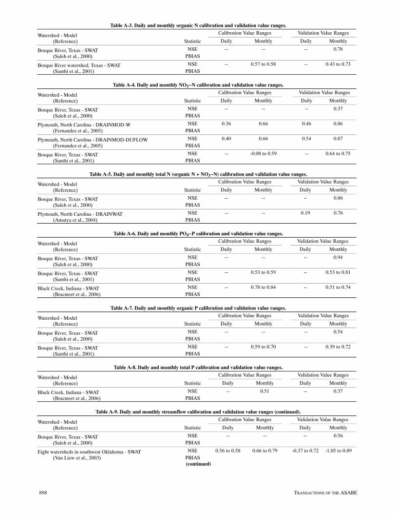
898 TRANSACTIONS OF THE ASABE
Table A-3. Daily and monthly organic N calibration and validation value ranges.
Watershed - Model(Reference)
Calibration Value Ranges Validation Value Ranges
Statistic Daily Monthly Daily Monthly
Bosque River, Texas - SWAT(Saleh et al., 2000)
NSE -- -- -- 0.78PBIAS
Bosque River watershed, Texas - SWAT(Santhi et al., 2001)
NSE -- 0.57 to 0.58 -- 0.43 to 0.73PBIAS
Table A-4. Daily and monthly NO3−N calibration and validation value ranges.
Watershed - Model(Reference)
Calibration Value Ranges Validation Value Ranges
Statistic Daily Monthly Daily Monthly
Bosque River, Texas - SWAT(Saleh et al., 2000)
NSE -- -- -- 0.37PBIAS
Plymouth, North Carolina - DRAINMOD-W(Fernandez et al., 2005)
NSE 0.36 0.66 0.46 0.86PBIAS
Plymouth, North Carolina - DRAINMOD-DUFLOW(Fernandez et al., 2005)
NSE 0.40 0.66 0.54 0.87PBIAS
Bosque River, Texas - SWAT(Santhi et al., 2001)
NSE -- -0.08 to 0.59 -- 0.64 to 0.75PBIAS
Table A-5. Daily and monthly total N (organic N + NO3−N) calibration and validation value ranges.
Watershed - Model(Reference)
Calibration Value Ranges Validation Value Ranges
Statistic Daily Monthly Daily Monthly
Bosque River, Texas - SWAT(Saleh et al., 2000)
NSE -- -- -- 0.86PBIAS
Plymouth, North Carolina - DRAINWAT(Amatya et al., 2004)
NSE -- -- 0.19 0.76PBIAS
Table A-6. Daily and monthly PO4−P calibration and validation value ranges.
Watershed - Model(Reference)
Calibration Value Ranges Validation Value Ranges
Statistic Daily Monthly Daily Monthly
Bosque River, Texas - SWAT(Saleh et al., 2000)
NSE -- -- -- 0.94PBIAS
Bosque River, Texas - SWAT(Santhi et al., 2001)
NSE -- 0.53 to 0.59 -- 0.53 to 0.81PBIAS
Black Creek, Indiana - SWAT(Bracmort et al., 2006)
NSE -- 0.78 to 0.84 -- 0.51 to 0.74PBIAS
Table A-7. Daily and monthly organic P calibration and validation value ranges.
Watershed - Model(Reference)
Calibration Value Ranges Validation Value Ranges
Statistic Daily Monthly Daily Monthly
Bosque River, Texas - SWAT(Saleh et al., 2000)
NSE -- -- -- 0.54PBIAS
Bosque River, Texas - SWAT(Santhi et al., 2001)
NSE -- 0.59 to 0.70 -- 0.39 to 0.72PBIAS
Table A-8. Daily and monthly total P calibration and validation value ranges.
Watershed - Model(Reference)
Calibration Value Ranges Validation Value Ranges
Statistic Daily Monthly Daily Monthly
Black Creek, Indiana - SWAT(Bracmort et al., 2006)
NSE -- 0.51 -- 0.37PBIAS
Table A-9. Daily and monthly streamflow calibration and validation value ranges (continued).
Watershed - Model(Reference)
Calibration Value Ranges Validation Value Ranges
Statistic Daily Monthly Daily Monthly
Bosque River, Texas - SWAT(Saleh et al., 2000)
NSE -- -- -- 0.56PBIAS
Eight watersheds in southwest Oklahoma - SWAT(Van Liew et al., 2003)
NSE 0.56 to 0.58 0.66 to 0.79 -0.37 to 0.72 -1.05 to 0.89PBIAS(continued)
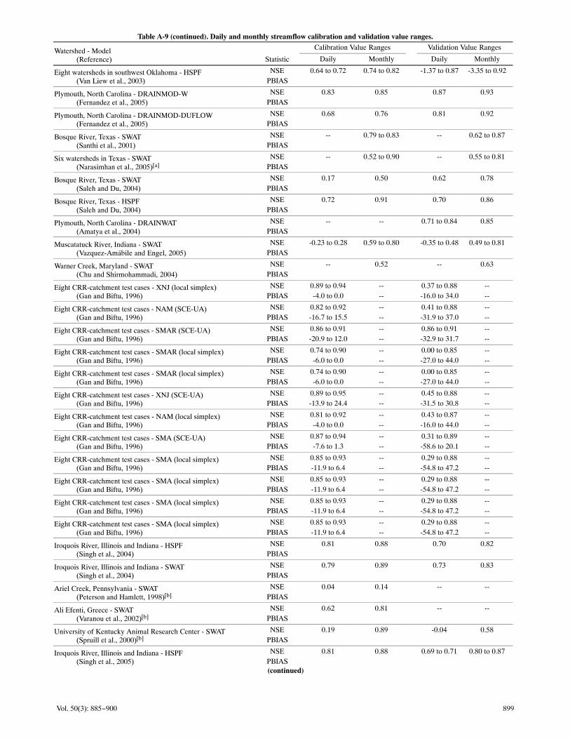
899Vol. 50(3): 885−900
Table A-9 (continued). Daily and monthly streamflow calibration and validation value ranges.
Watershed - Model(Reference)
Calibration Value Ranges Validation Value Ranges
Statistic Daily Monthly Daily Monthly
Eight watersheds in southwest Oklahoma - HSPF(Van Liew et al., 2003)
NSE 0.64 to 0.72 0.74 to 0.82 -1.37 to 0.87 -3.35 to 0.92PBIAS
Plymouth, North Carolina - DRAINMOD-W(Fernandez et al., 2005)
NSE 0.83 0.85 0.87 0.93PBIAS
Plymouth, North Carolina - DRAINMOD-DUFLOW(Fernandez et al., 2005)
NSE 0.68 0.76 0.81 0.92PBIAS
Bosque River, Texas - SWAT(Santhi et al., 2001)
NSE -- 0.79 to 0.83 -- 0.62 to 0.87PBIAS
Six watersheds in Texas - SWAT(Narasimhan et al., 2005)[a]
NSE -- 0.52 to 0.90 -- 0.55 to 0.81PBIAS
Bosque River, Texas - SWAT(Saleh and Du, 2004)
NSE 0.17 0.50 0.62 0.78PBIAS
Bosque River, Texas - HSPF(Saleh and Du, 2004)
NSE 0.72 0.91 0.70 0.86PBIAS
Plymouth, North Carolina - DRAINWAT(Amatya et al., 2004)
NSE -- -- 0.71 to 0.84 0.85PBIAS
Muscatatuck River, Indiana - SWAT(Vazquez-Amábile and Engel, 2005)
NSE -0.23 to 0.28 0.59 to 0.80 -0.35 to 0.48 0.49 to 0.81PBIAS
Warner Creek, Maryland - SWAT(Chu and Shirmohammadi, 2004)
NSE -- 0.52 -- 0.63PBIAS
Eight CRR-catchment test cases - XNJ (local simplex)(Gan and Biftu, 1996)
NSE 0.89 to 0.94 -- 0.37 to 0.88 --PBIAS -4.0 to 0.0 -- -16.0 to 34.0 --
Eight CRR-catchment test cases - NAM (SCE-UA)(Gan and Biftu, 1996)
NSE 0.82 to 0.92 -- 0.41 to 0.88 --PBIAS -16.7 to 15.5 -- -31.9 to 37.0 --
Eight CRR-catchment test cases - SMAR (SCE-UA)(Gan and Biftu, 1996)
NSE 0.86 to 0.91 -- 0.86 to 0.91 --PBIAS -20.9 to 12.0 -- -32.9 to 31.7 --
Eight CRR-catchment test cases - SMAR (local simplex)(Gan and Biftu, 1996)
NSE 0.74 to 0.90 -- 0.00 to 0.85 --PBIAS -6.0 to 0.0 -- -27.0 to 44.0 --
Eight CRR-catchment test cases - SMAR (local simplex)(Gan and Biftu, 1996)
NSE 0.74 to 0.90 -- 0.00 to 0.85 --PBIAS -6.0 to 0.0 -- -27.0 to 44.0 --
Eight CRR-catchment test cases - XNJ (SCE-UA)(Gan and Biftu, 1996)
NSE 0.89 to 0.95 -- 0.45 to 0.88 --PBIAS -13.9 to 24.4 -- -31.5 to 30.8 --
Eight CRR-catchment test cases - NAM (local simplex)(Gan and Biftu, 1996)
NSE 0.81 to 0.92 -- 0.43 to 0.87 --PBIAS -4.0 to 0.0 -- -16.0 to 44.0 --
Eight CRR-catchment test cases - SMA (SCE-UA)(Gan and Biftu, 1996)
NSE 0.87 to 0.94 -- 0.31 to 0.89 --PBIAS -7.6 to 1.3 -- -58.6 to 20.1 --
Eight CRR-catchment test cases - SMA (local simplex)(Gan and Biftu, 1996)
NSE 0.85 to 0.93 -- 0.29 to 0.88 --PBIAS -11.9 to 6.4 -- -54.8 to 47.2 --
Eight CRR-catchment test cases - SMA (local simplex)(Gan and Biftu, 1996)
NSE 0.85 to 0.93 -- 0.29 to 0.88 --PBIAS -11.9 to 6.4 -- -54.8 to 47.2 --
Eight CRR-catchment test cases - SMA (local simplex)(Gan and Biftu, 1996)
NSE 0.85 to 0.93 -- 0.29 to 0.88 --PBIAS -11.9 to 6.4 -- -54.8 to 47.2 --
Eight CRR-catchment test cases - SMA (local simplex)(Gan and Biftu, 1996)
NSE 0.85 to 0.93 -- 0.29 to 0.88 --PBIAS -11.9 to 6.4 -- -54.8 to 47.2 --
Iroquois River, Illinois and Indiana - HSPF(Singh et al., 2004)
NSE 0.81 0.88 0.70 0.82PBIAS
Iroquois River, Illinois and Indiana - SWAT(Singh et al., 2004)
NSE 0.79 0.89 0.73 0.83PBIAS
Ariel Creek, Pennsylvania - SWAT(Peterson and Hamlett, 1998)[b]
NSE 0.04 0.14 -- --PBIAS
Ali Efenti, Greece - SWAT(Varanou et al., 2002)[b]
NSE 0.62 0.81 -- --PBIAS
University of Kentucky Animal Research Center - SWAT(Spruill et al., 2000)[b]
NSE 0.19 0.89 -0.04 0.58PBIAS
Iroquois River, Illinois and Indiana - HSPF(Singh et al., 2005)
NSE 0.81 0.88 0.69 to 0.71 0.80 to 0.87PBIAS(continued)

900 TRANSACTIONS OF THE ASABE
Table A-9 (continued). Daily and monthly streamflow calibration and validation value ranges.
Watershed - Model(Reference)
Calibration Value Ranges Validation Value Ranges
Statistic Daily Monthly Daily Monthly
Iroquois River, Illinois and Indiana - SWAT(Singh et al., 2005)
NSE 0.79 0.88 0.70 to 0.83 0.80 to 0.93PBIAS
Black Creek, Indiana - SWAT(Bracmort et al., 2006)
NSE -- 0.73 to 0.84 -- 0.63 to 0.73PBIAS
Five USDA-ARS experimental watersheds - SWAT(Van Liew et al., 2007)
NSE 0.30 to 0.76 0.48 to 0.90 -1.81 to 0.68 -2.50 to 0.89PBIAS 2.9 to -91.7 -- 2.7 to -155.6 --
[a] Weekly values.[b] In Borah and Bera (2004).