Embed Size (px)
Citation preview


This page intentionally left blank
LONDON MATHEMATICAL SOCIETY LECTURE NOTE SERIESManaging Editor: Professor M. Reid, Mathematics Institute, University of Warwick, Coventry CV47AL, United Kingdom
The titles below are available from booksellers, or from Cambridge University Press atwww.cambridge.org/mathematics
216 Stochastic partial differential equations, A. ETHERIDGE (ed)217 Quadratic forms with applications to algebraic geometry and topology, A. PFISTER218 Surveys in combinatorics, 1995, P. ROWLINSON (ed)220 Algebraic set theory, A. JOYAL & I. MOERDIJK221 Harmonic approximation, S.J. GARDINER222 Advances in linear logic, J.-Y. GIRARD, Y. LAFONT & L. REGNIER (eds)223 Analytic semigroups and semilinear initial boundary value problems, K. TAIRA224 Computability, enumerability, unsolvability, S.B. COOPER, T.A. SLAMAN & S.S. WAINER (eds)225 A mathematical introduction to string theory, S. ALBEVERIO et al226 Novikov conjectures, index theorems and rigidity I, S.C. FERRY, A. RANICKI & J. ROSENBERG
(eds)227 Novikov conjectures, index theorems and rigidity II, S.C. FERRY, A. RANICKI &
J. ROSENBERG (eds)
228 Ergodic theory of Zd actions, M. POLLICOTT & K. SCHMIDT (eds)229 Ergodicity for infinite dimensional systems, G. DA PRATO & J. ZABCZYK230 Prolegomena to a middlebrow arithmetic of curves of genus 2, J.W.S. CASSELS & E.V. FLYNN231 Semigroup theory and its applications, K.H. HOFMANN & M.W. MISLOVE (eds)232 The descriptive set theory of Polish group actions, H. BECKER & A.S. KECHRIS233 Finite fields and applications, S. COHEN & H. NIEDERREITER (eds)234 Introduction to subfactors, V. JONES & V.S. SUNDER235 Number theory: Seminaire de theorie des nombres de Paris 1993-94, S. DAVID (ed)236 The James forest, H. FETTER & B.G. DE BUEN237 Sieve methods, exponential sums, and their applications in number theory, G.R.H. GREAVES et al
(eds)238 Representation theory and algebraic geometry, A. MARTSINKOVSKY & G. TODOROV (eds)240 Stable groups, F.O. WAGNER241 Surveys in combinatorics, 1997, R.A. BAILEY (ed)242 Geometric Galois actions I, L. SCHNEPS & P. LOCHAK (eds)243 Geometric Galois actions II, L. SCHNEPS & P. LOCHAK (eds)244 Model theory of groups and automorphism groups, D.M. EVANS (ed)245 Geometry, combinatorial designs and related structures, J.W.P. HIRSCHFELD et al (eds)246 p-Automorphisms of finite p-groups, E.I. KHUKHRO247 Analytic number theory, Y. MOTOHASHI (ed)248 Tame topology and O-minimal structures, L. VAN DEN DRIES249 The atlas of finite groups - ten years on, R.T. CURTIS & R.A. WILSON (eds)250 Characters and blocks of finite groups, G. NAVARRO251 Grobner bases and applications, B. BUCHBERGER & F. WINKLER (eds)252 Geometry and cohomology in group theory, P.H. KROPHOLLER, G.A. NIBLO & R. STOHR (eds)253 The q-Schur algebra, S. DONKIN254 Galois representations in arithmetic algebraic geometry, A.J. SCHOLL & R.L. TAYLOR (eds)255 Symmetries and integrability of difference equations, P.A. CLARKSON & F.W. NIJHOFF (eds)256 Aspects of Galois theory, H. VOLKLEIN, J.G. THOMPSON, D. HARBATER & P. MULLER (eds)257 An introduction to noncommutative differential geometry and its physical applications (2nd
edition), J. MADORE258 Sets and proofs, S.B. COOPER & J.K. TRUSS (eds)259 Models and computability, S.B. COOPER & J. TRUSS (eds)260 Groups St Andrews 1997 in Bath I, C.M. CAMPBELL et al (eds)261 Groups St Andrews 1997 in Bath II, C.M. CAMPBELL et al (eds)262 Analysis and logic, C.W. HENSON, J. IOVINO, A.S. KECHRIS & E. ODELL263 Singularity theory, W. BRUCE & D. MOND (eds)264 New trends in algebraic geometry, K. HULEK, F. CATANESE, C. PETERS & M. REID (eds)265 Elliptic curves in cryptography, I. BLAKE, G. SEROUSSI & N. SMART267 Surveys in combinatorics, 1999, J.D. LAMB & D.A. PREECE (eds)268 Spectral asymptotics in the semi-classical limit, M. DIMASSI & J. SJOSTRAND269 Ergodic theory and topological dynamics of group actions on homogeneous spaces, M.B. BEKKA
& M. MAYER271 Singular perturbations of differential operators, S. ALBEVERIO & P. KURASOV272 Character theory for the odd order theorem, T. PETERFALVI. Translated by R. SANDLING273 Spectral theory and geometry, E.B. DAVIES & Y. SAFAROV (eds)274 The Mandelbrot set, theme and variations, T. LEI (ed)275 Descriptive set theory and dynamical systems, M. FOREMAN, A.S. KECHRIS, A. LOUVEAU &
B. WEISS (eds)276 Singularities of plane curves, E. CASAS-ALVERO277 Computational and geometric aspects of modern algebra, M. ATKINSON et al (eds)278 Global attractors in abstract parabolic problems, J.W. CHOLEWA & T. DLOTKO279 Topics in symbolic dynamics and applications, F. BLANCHARD, A. MAASS & A. NOGUEIRA
(eds)280 Characters and automorphism groups of compact Riemann surfaces, T. BREUER281 Explicit birational geometry of 3-folds, A. CORTI & M. REID (eds)282 Auslander-Buchweitz approximations of equivariant modules, M. HASHIMOTO283 Nonlinear elasticity, Y.B. FU & R.W. OGDEN (eds)284 Foundations of computational mathematics, R. DEVORE, A. ISERLES & E. SULI (eds)285 Rational points on curves over finite fields, H. NIEDERREITER & C. XING286 Clifford algebras and spinors (2nd Edition), P. LOUNESTO287 Topics on Riemann surfaces and Fuchsian groups, E. BUJALANCE, A.F. COSTA & E.
MARTINEZ (eds)288 Surveys in combinatorics, 2001, J.W.P. HIRSCHFELD (ed)289 Aspects of Sobolev-type inequalities, L. SALOFF-COSTE290 Quantum groups and Lie theory, A. PRESSLEY (ed)291 Tits buildings and the model theory of groups, K. TENT (ed)292 A quantum groups primer, S. MAJID
293 Second order partial differential equations in Hilbert spaces, G. DA PRATO & J. ZABCZYK294 Introduction to operator space theory, G. PISIER295 Geometry and integrability, L. MASON & Y. NUTKU (eds)296 Lectures on invariant theory, I. DOLGACHEV297 The homotopy category of simply connected 4-manifolds, H.-J. BAUES298 Higher operads, higher categories, T. LEINSTER (ed)299 Kleinian groups and hyperbolic 3-manifolds, Y. KOMORI, V. MARKOVIC & C. SERIES (eds)300 Introduction to Mobius differential geometry, U. HERTRICH-JEROMIN301 Stable modules and the D(2)-problem, F.E.A. JOHNSON302 Discrete and continuous nonlinear Schrodinger systems, M.J. ABLOWITZ, B. PRINARI & A.D.
TRUBATCH303 Number theory and algebraic geometry, M. REID & A. SKOROBOGATOV (eds)304 Groups St Andrews 2001 in Oxford I, C.M. CAMPBELL, E.F. ROBERTSON & G.C. SMITH (eds)305 Groups St Andrews 2001 in Oxford II, C.M. CAMPBELL, E.F. ROBERTSON & G.C. SMITH (eds)306 Geometric mechanics and symmetry, J. MONTALDI & T. RATIU (eds)307 Surveys in combinatorics 2003, C.D. WENSLEY (ed.)308 Topology, geometry and quantum field theory, U.L. TILLMANN (ed)309 Corings and comodules, T. BRZEZINSKI & R. WISBAUER310 Topics in dynamics and ergodic theory, S. BEZUGLYI & S. KOLYADA (eds)311 Groups: topological, combinatorial and arithmetic aspects, T.W. MULLER (ed)312 Foundations of computational mathematics, Minneapolis 2002, F. CUCKER et al (eds)313 Transcendental aspects of algebraic cycles, S. MULLER-STACH & C. PETERS (eds)314 Spectral generalizations of line graphs, D. CVETKOVIC, P. ROWLINSON & S. SIMIC315 Structured ring spectra, A. BAKER & B. RICHTER (eds)316 Linear logic in computer science, T. EHRHARD, P. RUET, J.-Y. GIRARD & P. SCOTT (eds)317 Advances in elliptic curve cryptography, I.F. BLAKE, G. SEROUSSI & N.P. SMART (eds)318 Perturbation of the boundary in boundary-value problems of partial differential equations, D.
HENRY319 Double affine Hecke algebras, I. CHEREDNIK320 L-functions and Galois representations, D. BURNS, K. BUZZARD & J. NEKOVAR (eds)321 Surveys in modern mathematics, V. PRASOLOV & Y. ILYASHENKO (eds)322 Recent perspectives in random matrix theory and number theory, F. MEZZADRI & N.C. SNAITH
(eds)323 Poisson geometry, deformation quantisation and group representations, S. GUTT et al (eds)324 Singularities and computer algebra, C. LOSSEN & G. PFISTER (eds)325 Lectures on the Ricci flow, P. TOPPING326 Modular representations of finite groups of Lie type, J.E. HUMPHREYS327 Surveys in combinatorics 2005, B.S. WEBB (ed)328 Fundamentals of hyperbolic manifolds, R. CANARY, D. EPSTEIN & A. MARDEN (eds)329 Spaces of Kleinian groups, Y. MINSKY, M. SAKUMA & C. SERIES (eds)330 Noncommutative localization in algebra and topology, A. RANICKI (ed)331 Foundations of computational mathematics, Santander 2005, L.M PARDO, A. PINKUS, E. SULI &
M.J. TODD (eds)332 Handbook of tilting theory, L. ANGELERI HUGEL, D. HAPPEL & H. KRAUSE (eds)333 Synthetic differential geometry (2nd Edition), A. KOCK334 The Navier-Stokes equations, N. RILEY & P. DRAZIN335 Lectures on the combinatorics of free probability, A. NICA & R. SPEICHER336 Integral closure of ideals, rings, and modules, I. SWANSON & C. HUNEKE337 Methods in Banach space theory, J. M. F. CASTILLO & W. B. JOHNSON (eds)338 Surveys in geometry and number theory, N. YOUNG (ed)339 Groups St Andrews 2005 I, C.M. CAMPBELL, M.R. QUICK, E.F. ROBERTSON & G.C. SMITH
(eds)340 Groups St Andrews 2005 II, C.M. CAMPBELL, M.R. QUICK, E.F. ROBERTSON & G.C. SMITH
(eds)341 Ranks of elliptic curves and random matrix theory, J.B. CONREY, D.W. FARMER, F.
MEZZADRI & N.C. SNAITH (eds)342 Elliptic cohomology, H.R. MILLER & D.C. RAVENEL (eds)343 Algebraic cycles and motives I, J. NAGEL & C. PETERS (eds)344 Algebraic cycles and motives II, J. NAGEL & C. PETERS (eds)345 Algebraic and analytic geometry, A. NEEMAN346 Surveys in combinatorics 2007, A. HILTON & J. TALBOT (eds)347 Surveys in contemporary mathematics, N. YOUNG & Y. CHOI (eds)348 Transcendental dynamics and complex analysis, P.J. RIPPON & G.M. STALLARD (eds)349 Model theory with applications to algebra and analysis I, Z. CHATZIDAKIS, D. MACPHERSON,
A. PILLAY & A. WILKIE (eds)350 Model theory with applications to algebra and analysis II, Z. CHATZIDAKIS, D. MACPHERSON,
A. PILLAY & A. WILKIE (eds)351 Finite von Neumann algebras and masas, A.M. SINCLAIR & R.R. SMITH352 Number theory and polynomials, J. MCKEE & C. SMYTH (eds)353 Trends in stochastic analysis, J. BLATH, P. MORTERS & M. SCHEUTZOW (eds)354 Groups and analysis, K. TENT (ed)355 Non-equilibrium statistical mechanics and turbulence, J. CARDY, G. FALKOVICH & K.
GAWEDZKI356 Elliptic curves and big Galois representations, D. DELBOURGO357 Algebraic theory of differential equations, M.A.H. MACCALLUM & A.V. MIKHAILOV (eds)358 Geometric and cohomological methods in group theory, M. BRIDSON, P. KROPHOLLER & I.
LEARY (eds)359 Moduli spaces and vector bundles, L. BRAMBILA-PAZ, S.B. BRADLOW, O. GARCIA-PRADA &
S. RAMANAN (eds)360 Zariski geometries, B. ZILBER361 Words: Notes on verbal width in groups, D. SEGAL362 Differential tensor algebras and their module categories, R. BAUTISTA, L. SALMERON & R.
ZUAZUA363 Foundations of computational mathematics, Hong Kong 2008, M.J. TODD, F. CUCKER & A.
PINKUS (eds)364 Partial differential equations and fluid mechanics, J.C. ROBINSON & J.L. RODRIGO (eds)365 Surveys in combinatorics 2009, S. HUCZYNSKA, J.D.MITCHELL & C.M.RONEY-DOUGAL (eds)366 Highly oscillatory problems, B. ENGQUIST, A. FOKAS, E. HAIRER & A. ISERLES (eds)

Partial Differential Equations andFluid Mechanics
Edited by
JAMES C. ROBINSON & JOSE L. RODRIGO
University of Warwick
c a m b r i d g e u n i v e r s i t y p r e s s
Cambridge, New York, Melbourne, Madrid, Cape Town, Singapore, Sao Paulo, Delhi
Cambridge University Press
The Edinburgh Building, Cambridge CB2 8RU, UK
Published in the United States of America by Cambridge University Press, New York
www.cambridge.org
Information on this title: www.cambridge.org/9780521125123
c© Cambridge University Press 2009
This publication is in copyright. Subject to statutory exception
and to the provisions of relevant collective licensing agreements,
no reproduction of any part may take place without
the written permission of Cambridge University Press.
First published 2009
Printed in the United Kingdom at the University Press, Cambridge
A catalogue record for this publication is available from the British Library
ISBN 978-0-521-12512-3 paperback
Cambridge University Press has no responsibility for the persistence or
accuracy of URLs for external or third-party Internet websites referred to
in this publication, and does not guarantee that any content on such
websites is, or will remain, accurate or appropriate.

To Tania and Elizabeth

Contents
Preface page ix
List of contributors x
1 Shear flows and their attractors
M. Boukrouche & G. �Lukaszewicz 1
2 Mathematical results concerning unsteady flows of
chemically reacting incompressible fluids
M. Bulıcek, J. Malek, & K.R. Rajagopal 26
3 The uniqueness of Lagrangian trajectories in
Navier–Stokes flows
M. Dashti & J.C. Robinson 54
4 Some controllability results in fluid mechanics
E. Fernandez-Cara 64
5 Singularity formation and separation phenomena in
boundary layer theory
F. Gargano, M.C. Lombardo, M. Sammartino, & V. Sciacca 81
6 Partial regularity results for solutions of the
Navier–Stokes system
I. Kukavica 121
7 Anisotropic Navier–Stokes equations in a bounded
cylindrical domain
M. Paicu & G. Raugel 146
8 The regularity problem for the three-dimensional
Navier–Stokes equations
J.C. Robinson & W. Sadowski 185
9 Contour dynamics for the surface quasi-geostrophic
equation
J.L. Rodrigo 207
10 Theory and applications of statistical solutions of the
Navier–Stokes equations
R. Rosa 228
vii

Preface
This volume is the result of a workshop, “Partial Differential Equationsand Fluid Mechanics”, which took place in the Mathematics Instituteat the University of Warwick, May 21st–23rd, 2007.
Several of the speakers agreed to write review papers related to theircontributions to the workshop, while others have written more tradi-tional research papers. All the papers have been carefully edited in theinterests of clarity and consistency, and the research papers have beenexternally refereed. We are very grateful to the referees for their work.We believe that this volume therefore provides an accessible summaryof a wide range of active research topics, along with some exciting newresults, and we hope that it will prove a useful resource for both graduatestudents new to the area and to more established researchers.
We would like to express their gratitude to the following sponsors ofthe workshop: the London Mathematical Society, the Royal Society, viaa University Research Fellowship awarded to James Robinson, the NorthAmerican Fund and Research Development Fund schemes of WarwickUniversity, and the Warwick Mathematics Department (via MIR@W).JCR is currently supported by the EPSRC, grant EP/G007470/1.
Finally it is a pleasure to thank Yvonne Collins and Hazel Higgensfrom the Warwick Mathematics Research Centre for their assistanceduring the organization of the workshop.
Warwick, James C. RobinsonDecember 2008 Jose L. Rodrigo
ix
Contributors
Those contributors who presented their work at the Warwick meetingare indicated by a star in the following list.
Mahdi BoukroucheLaboratory of Mathematics, University of Saint-Etienne, LaMUSE EA-3989, 23 rue du Dr Paul Michelon, Saint-Etienne, 42023. [email protected]
Miroslav BulıcekCharles University, Faculty of Mathematics and Physics, MathematicalInstitute, Sokolovska 83, 186 75 Prague 8. Czech [email protected]
Masoumeh Dashti �
Mathematics Department, University of Warwick, Coventry, CV47AL.United [email protected]
Enrique Fernandez-Cara �
Departamento de Ecuaciones Diferenciales y Analisis Numerico,Facultad de Matematicas, Universidad de Sevilla, Apartado 1160, 41080Sevilla. [email protected]
Francesco GarganoDepartment of Mathematics, Via Archirafi 34, 90123 Palermo. [email protected]
x
List of contributors xi
Igor Kukavica �
Department of Mathematics, University of Southern California,Los Angeles, CA 90089. [email protected]
Maria Carmela LombardoDepartment of Mathematics, Via Archirafi 34, 90123 Palermo. [email protected]
Grzegorz �Lukaszewicz �
University of Warsaw, Mathematics Department, ul. Banacha 2, 02-957,Warsaw. [email protected]
Josef Malek �
Charles University, Faculty of Mathematics and Physics, MathematicalInstitute, Sokolovska 83, 186 75 Prague 8. Czech [email protected]
Marius PaicuUniversite Paris-Sud and CNRS, Laboratoire de Mathematiques, OrsayCedex, F-91405. [email protected]
Kumbakonam R. RajagopalDepartment of Mechanical Engineering, Texas A&M University, CollegeStation, TX 77843. [email protected]
Genevieve Raugel �
CNRS and Universite Paris-Sud, Laboratoire de Mathematiques, OrsayCedex, F-91405. [email protected]
James C. RobinsonMathematics Institute, University of Warwick, Coventry, CV4 7AL.United [email protected]
Jose L. Rodrigo �
Mathematics Department, University of Warwick, Coventry, CV4 7AL.United [email protected]
xii List of contributors
Ricardo M.S. Rosa �
Instituto de Matematica, Universidade Federal do Rio de Janeiro , CaixaPostal 68530 Ilha do Fundao, Rio de Janeiro, RJ 21945-970. [email protected]
Witold Sadowski �
Faculty of Mathematics, Informatics and Mechanics, University ofWarsaw, Banacha 2, 02-097 Warszawa. [email protected]
Marco Sammartino �
Department of Mathematics, Via Archirafi 34, 90123 Palermo. [email protected]
Vincenzo SciaccaDepartment of Mathematics, Via Archirafi 34, 90123 Palermo. [email protected]
1
Shear flows and their attractorsMahdi Boukrouche
Laboratory of Mathematics, University of Saint-Etienne,LaMUSE EA-3989, 23 rue du Dr Paul Michelon,
Saint-Etienne, 42023. [email protected]
Grzegorz �LukaszewiczUniversity of Warsaw, Mathematics Department,
ul. Banacha 2, 02-957 Warsaw. [email protected]
Abstract
We consider the problem of the existence and finite dimensionalityof attractors for some classes of two-dimensional turbulent boundary-driven flows that naturally appear in lubrication theory. The flows admitmixed, non-standard boundary conditions and time-dependent drivingforces. We are interested in the dependence of the dimension of theattractors on the geometry of the flow domain and on the boundaryconditions.
1.1 Introduction
This work gives a survey of the results obtained in a series of papersby Boukrouche & �Lukaszewicz (2004, 2005a,b, 2007) and Boukrouche,�Lukaszewicz, & Real (2006) in which we consider the problem of theexistence and finite dimensionality of attractors for some classes of two-dimensional turbulent boundary-driven flows (Problems I–IV below).The flows admit mixed, non-standard boundary conditions and alsotime-dependent driving forces (Problems III and IV). We are interestedin the dependence of the dimension of the attractors on the geometryof the flow domain and on the boundary conditions. This research ismotivated by problems from lubrication theory. Our results generalizesome earlier ones devoted to the existence of attractors and estimates oftheir dimensions for a variety of Navier–Stokes flows. We would like tomention a few results that are particularly relevant to the problems weconsider.
Most earlier results on shear flows treated the autonomous Navier–Stokes equations. In Doering & Wang (1998), the domain of the flow is
Published in Partial Differential Equations and Fluid Mechanics, edited byJames C. Robinson and Jose L. Rodrigo. c© Cambridge University Press 2009.
2 M. Boukrouche & G. �Lukaszewicz
an elongated rectangle Ω = (0, L) × (0, h), L � h. Boundary condi-tions of Dirichlet type are assumed on the bottom and the top partsof the boundary and a periodic boundary condition is assumed on thelateral part of the boundary. In this case the attractor dimension can beestimated from above by cL
hRe3/2, where c is a universal constant, and
Re = Uhν is the Reynolds number. Ziane (1997) gave optimal bounds for
the attractor dimension for a flow in a rectangle (0, 2πL) × (0, 2πL/α),with periodic boundary conditions and given external forcing. The esti-mates are of the form c0/α ≤ dimA ≤ c1/α, see also Miranville & Ziane(1997). Some free boundary conditions are considered by Ziane (1998),see also Temam & Ziane (1998), and an upper bound on the attrac-tor dimension established with the use of a suitable anisotropic versionof the Lieb-Thirring inequality, in a similar way to Doering & Wang(1998). Dirichlet-periodic and free-periodic boundary conditions anddomains with more general geometry were considered by Boukrouche &�Lukaszewicz (2004, 2005a,b) where still other forms of the Lieb-Thirringinequality were established to study the dependence of the attractordimension on the shape of the domain of the flow. The Navier slip bound-ary condition and the case of an unbounded domain were consideredrecently by Mucha & Sadowski (2005).
Boundary-driven flows in smooth and bounded two-dimensionaldomains for a non-autonomous Navier–Stokes system are consideredby Miranville & Wang (1997), using an approach developed by Chep-yzhov & Vishik (see their 2002 monograph for details). An extension tosome unbounded domains can be found in Moise, Rosa, & Wang (2004),cf. also �Lukaszewicz & Sadowski (2004).
Other related problems can be found, for example, in the monographsby Chepyzhov & Vishik (2002), Doering & Gibbon (1995), Foias et al.(2001), Robinson (2001), and Temam (1997), and the literature quotedthere.
Formulation of the problems considered.
We consider the two-dimensional Navier–Stokes equations,
ut − νΔu+ (u · ∇)u+ ∇p = 0 (1.1)
and
div u = 0 (1.2)
in the channel
Ω∞ = {x = (x1, x2) : −∞ < x1 <∞, 0 < x2 < h(x1)},
Shear flows and their attractors 3
where the function h is positive, smooth, and L-periodic in x1.Let
Ω = {x = (x1, x2) : 0 < x1 < L, 0 < x2 < h(x1)}and ∂Ω = Γ0 ∪ ΓL ∪ Γ1, where Γ0 and Γ1 are the bottom and the top,and ΓL is the lateral part of the boundary of Ω.
We are interested in solutions of (1.1)–(1.2) in Ω that are L-periodicwith respect to x1 and satisfy the initial condition
u(x, 0) = u0(x) for x ∈ Ω, (1.3)
together with the following boundary conditions on the bottom and onthe top parts, Γ0 and Γ1, of the domain Ω.
Case I. We assume that
u = 0 on Γ1 (1.4)
(non-penetration) and
u = U0e1 = (U0, 0) on Γ0. (1.5)
Case II. We assume that
u.n = 0 and τ · σ(u, p) · n = 0 on Γ1, (1.6)
i.e. the tangential component of the normal stress tensor σ · n vanisheson Γ1. The components of the stress tensor σ are
σij(u, p) = ν
(∂ui
∂xj+∂uj
∂xi
)− p δij , 1 ≤ i, j ≤ 3, (1.7)
where δij is the Kronecker symbol. As for case I, we set
u = U0e1 = (U0, 0) on Γ0. (1.8)
Case III. We assume that
u = 0 on Γ1 and (1.9)
u = U0(t)e1 = (U0(t), 0) on Γ0, (1.10)
where U0(t) is a locally Lipschitz continuous function of time t.
Case IV. We assume that
u = 0 on Γ1. (1.11)
4 M. Boukrouche & G. �Lukaszewicz
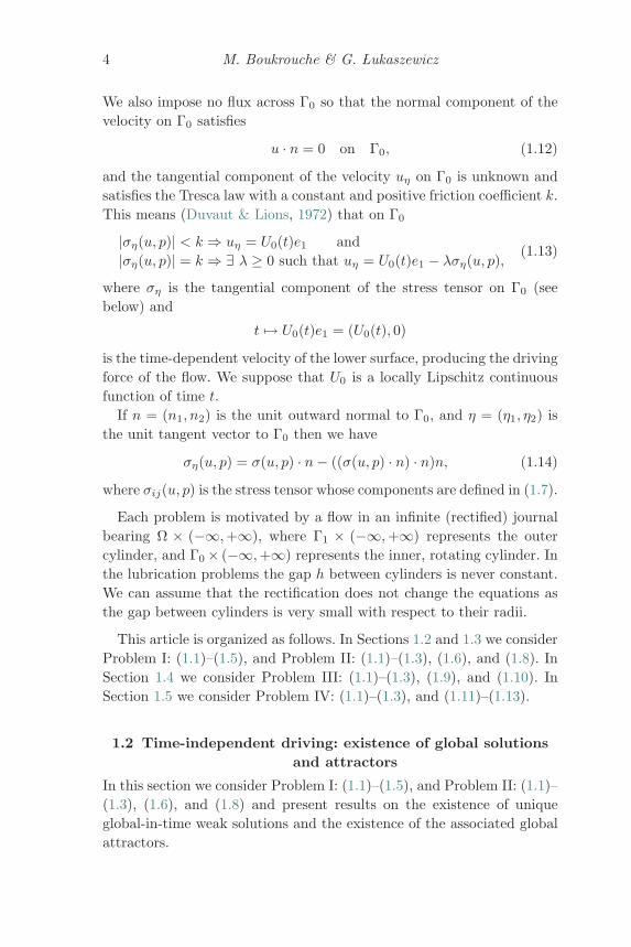
We also impose no flux across Γ0 so that the normal component of thevelocity on Γ0 satisfies
u · n = 0 on Γ0, (1.12)
and the tangential component of the velocity uη on Γ0 is unknown andsatisfies the Tresca law with a constant and positive friction coefficient k.This means (Duvaut & Lions, 1972) that on Γ0
|ση(u, p)| < k ⇒ uη = U0(t)e1 and|ση(u, p)| = k ⇒ ∃ λ ≥ 0 such that uη = U0(t)e1 − λση(u, p),
(1.13)
where ση is the tangential component of the stress tensor on Γ0 (seebelow) and
t �→ U0(t)e1 = (U0(t), 0)
is the time-dependent velocity of the lower surface, producing the drivingforce of the flow. We suppose that U0 is a locally Lipschitz continuousfunction of time t.
If n = (n1, n2) is the unit outward normal to Γ0, and η = (η1, η2) isthe unit tangent vector to Γ0 then we have
ση(u, p) = σ(u, p) · n− ((σ(u, p) · n) · n)n, (1.14)
where σij(u, p) is the stress tensor whose components are defined in (1.7).
Each problem is motivated by a flow in an infinite (rectified) journalbearing Ω × (−∞,+∞), where Γ1 × (−∞,+∞) represents the outercylinder, and Γ0 × (−∞,+∞) represents the inner, rotating cylinder. Inthe lubrication problems the gap h between cylinders is never constant.We can assume that the rectification does not change the equations asthe gap between cylinders is very small with respect to their radii.
This article is organized as follows. In Sections 1.2 and 1.3 we considerProblem I: (1.1)–(1.5), and Problem II: (1.1)–(1.3), (1.6), and (1.8). InSection 1.4 we consider Problem III: (1.1)–(1.3), (1.9), and (1.10). InSection 1.5 we consider Problem IV: (1.1)–(1.3), and (1.11)–(1.13).
1.2 Time-independent driving: existence of global solutionsand attractors
In this section we consider Problem I: (1.1)–(1.5), and Problem II: (1.1)–(1.3), (1.6), and (1.8) and present results on the existence of uniqueglobal-in-time weak solutions and the existence of the associated globalattractors.
Shear flows and their attractors 5
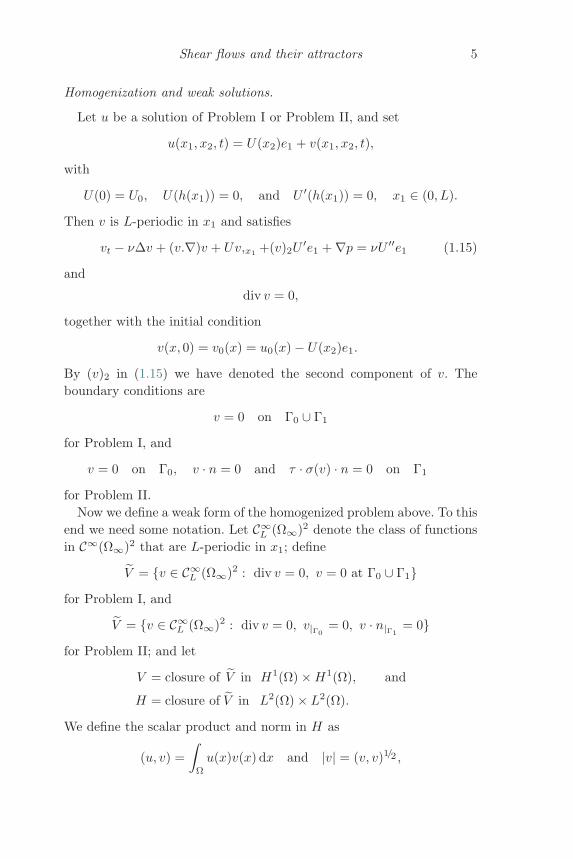
Homogenization and weak solutions.
Let u be a solution of Problem I or Problem II, and set
u(x1, x2, t) = U(x2)e1 + v(x1, x2, t),
with
U(0) = U0, U(h(x1)) = 0, and U ′(h(x1)) = 0, x1 ∈ (0, L).
Then v is L-periodic in x1 and satisfies
vt − νΔv + (v.∇)v + Uv,x1 +(v)2U ′e1 + ∇p = νU ′′e1 (1.15)
and
div v = 0,
together with the initial condition
v(x, 0) = v0(x) = u0(x) − U(x2)e1.
By (v)2 in (1.15) we have denoted the second component of v. Theboundary conditions are
v = 0 on Γ0 ∪ Γ1
for Problem I, and
v = 0 on Γ0, v · n = 0 and τ · σ(v) · n = 0 on Γ1
for Problem II.Now we define a weak form of the homogenized problem above. To this
end we need some notation. Let C∞L (Ω∞)2 denote the class of functions
in C∞(Ω∞)2 that are L-periodic in x1; define
V = {v ∈ C∞L (Ω∞)2 : div v = 0, v = 0 at Γ0 ∪ Γ1}
for Problem I, and
V = {v ∈ C∞L (Ω∞)2 : div v = 0, v|Γ0
= 0, v · n|Γ1= 0}
for Problem II; and let
V = closure of V in H1(Ω) ×H1(Ω), and
H = closure of V in L2(Ω) × L2(Ω).
We define the scalar product and norm in H as
(u, v) =∫
Ω
u(x)v(x) dx and |v| = (v, v)1/2 ,
6 M. Boukrouche & G. �Lukaszewicz
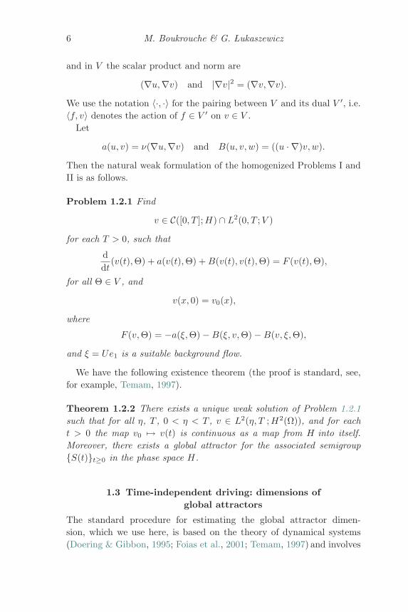
and in V the scalar product and norm are
(∇u,∇v) and |∇v|2 = (∇v,∇v).
We use the notation 〈·, ·〉 for the pairing between V and its dual V ′, i.e.〈f, v〉 denotes the action of f ∈ V ′ on v ∈ V .
Let
a(u, v) = ν(∇u,∇v) and B(u, v, w) = ((u · ∇)v, w).
Then the natural weak formulation of the homogenized Problems I andII is as follows.
Problem 1.2.1 Find
v ∈ C([0, T ];H) ∩ L2(0, T ;V )
for each T > 0, such that
ddt
(v(t),Θ) + a(v(t),Θ) +B(v(t), v(t),Θ) = F (v(t),Θ),
for all Θ ∈ V , and
v(x, 0) = v0(x),
where
F (v,Θ) = −a(ξ,Θ) −B(ξ, v,Θ) −B(v, ξ,Θ),
and ξ = Ue1 is a suitable background flow.
We have the following existence theorem (the proof is standard, see,for example, Temam, 1997).
Theorem 1.2.2 There exists a unique weak solution of Problem 1.2.1such that for all η, T , 0 < η < T , v ∈ L2(η, T ;H2(Ω)), and for eacht > 0 the map v0 �→ v(t) is continuous as a map from H into itself.Moreover, there exists a global attractor for the associated semigroup{S(t)}t≥0 in the phase space H.
1.3 Time-independent driving: dimensions ofglobal attractors
The standard procedure for estimating the global attractor dimen-sion, which we use here, is based on the theory of dynamical systems(Doering & Gibbon, 1995; Foias et al., 2001; Temam, 1997) and involves
Shear flows and their attractors 7
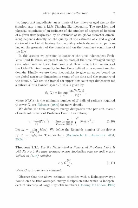
two important ingredients: an estimate of the time-averaged energy dis-sipation rate ε and a Lieb–Thirring-like inequality. The precision andphysical soundness of an estimate of the number of degrees of freedomof a given flow (expressed by an estimate of its global attractor dimen-sion) depends directly on the quality of the estimate of ε and a goodchoice of the Lieb–Thirring-like inequality which depends, in particu-lar, on the geometry of the domain and on the boundary conditions ofthe flow.
In this section we continue to consider the time-independent Prob-lems I and II. First, we present an estimate of the time-averaged energydissipation rate of these two flows and then present two versions ofthe Lieb–Thirring inequality for functions defined on a non-rectangulardomain. Finally we use these inequalities to give an upper bound onthe global attractor dimension in terms of the data and the geometry ofthe domain. We use the fractal (or upper box-counting) dimension: fora subset X of a Banach space B, this is given by
df (X) = lim supε→0
logN(X, ε)− log ε
,
where N(X, ε) is the minimum number of B-balls of radius ε requiredto cover X, see Falconer (1990) for more details.
We define the time-averaged energy dissipation rate per unit mass εof weak solutions u of Problems I and II as follows,
ε =ν
|Ω| 〈|∇u|2〉 : = lim sup
T→+∞ν
|Ω|1T
∫ T
0
|∇u(t)|2 dt. (1.16)
Let h0 = min0≤x1≤L
h(x1). We define the Reynolds number of the flow u
by Re = (h0U0)/ν. Then we have (Boukrouche & �Lukaszewicz, 2004,2005a):
Theorem 1.3.1 For the Navier–Stokes flows u of Problems I and IIwith Re >> 1 the time-averaged energy dissipation rate per unit mass εdefined in (1.16) satisfies
ε ≤ CU3
0
h0, (1.17)
where C is a numerical constant.
Observe that the above estimate coincides with a Kolmogorov-typebound on the time-averaged energy-dissipation rate which is indepen-dent of viscosity at large Reynolds numbers (Doering & Gibbon, 1995;
8 M. Boukrouche & G. �Lukaszewicz
Foias et al., 2001). Estimate (1.17) is the same as that obtained ear-lier for a rectangular domain by Doering & Constantin (1991) who useda background flow suitable for the channel case (see also Doering &Gibbon, 1995).
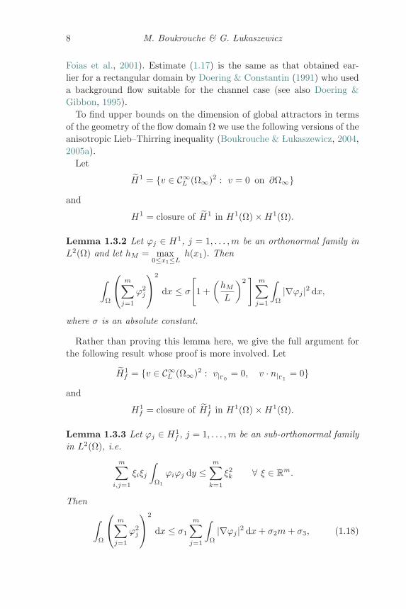
To find upper bounds on the dimension of global attractors in termsof the geometry of the flow domain Ω we use the following versions of theanisotropic Lieb–Thirring inequality (Boukrouche & �Lukaszewicz, 2004,2005a).
Let
H1 = {v ∈ C∞L (Ω∞)2 : v = 0 on ∂Ω∞}
and
H1 = closure of H1 in H1(Ω) ×H1(Ω).
Lemma 1.3.2 Let ϕj ∈ H1, j = 1, . . . ,m be an orthonormal family inL2(Ω) and let hM = max
0≤x1≤Lh(x1). Then
∫Ω
⎛⎝ m∑j=1
ϕ2j
⎞⎠2
dx ≤ σ
[1 +
(hM
L
)2]
m∑j=1
∫Ω
|∇ϕj |2 dx,
where σ is an absolute constant.
Rather than proving this lemma here, we give the full argument forthe following result whose proof is more involved. Let
H1f = {v ∈ C∞
L (Ω∞)2 : v|Γ0= 0, v · n|Γ1
= 0}and
H1f = closure of H1
f in H1(Ω) ×H1(Ω).
Lemma 1.3.3 Let ϕj ∈ H1f , j = 1, . . . ,m be an sub-orthonormal family
in L2(Ω), i.e.
m∑i,j=1
ξiξj
∫Ω1
ϕiϕj dy ≤m∑
k=1
ξ2k ∀ ξ ∈ Rm.
Then ∫Ω
⎛⎝ m∑j=1
ϕ2j
⎞⎠2
dx ≤ σ1
m∑j=1
∫Ω
|∇ϕj |2 dx+ σ2m+ σ3, (1.18)
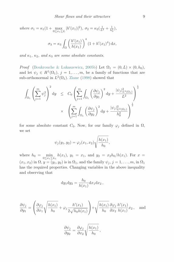
Shear flows and their attractors 9
where σ1 = κ1(1 + max0≤x1≤L
|h′(x1)|2), σ2 = κ2( 1L2 + 1
h20),
σ3 = κ3
∫Ω
(h′(x1)h(x1)
)4
(1 + h′(x1)4) dx,
and κ1, κ2, and κ3 are some absolute constants.
Proof (Boukrouche & �Lukaszewicz, 2005b) Let Ω1 = (0, L) × (0, h0),and let ψj ∈ H1(Ω1), j = 1, . . . ,m, be a family of functions that aresub-orthonormal in L2(Ω1). Ziane (1998) showed that
∫Ω1
⎛⎝ m∑j=1
ψ2j
⎞⎠2
dy ≤ C0
⎛⎝ m∑j=1
∫Ω1
(∂ψj
∂y1
)2
dy +|ψj |2L2(Ω1)
L2
⎞⎠12
×⎛⎝ m∑
j=1
∫Ω1
(∂ψj
∂y2
)2
dy +|ψj |2L2(Ω1)
h20
⎞⎠12
for some absolute constant C0. Now, for our family ϕj defined in Ω,we set
ψj(y1, y2) = ϕj(x1, x2)
√h(x1)h0
,
where h0 = min0≤x1≤L1
h(x1), y1 = x1, and y2 = x2h0/h(x1). For x =
(x1, x2) in Ω, y = (y1, y2) is in Ω1, and the family ψj , j = 1, . . . ,m, in Ω1
has the required properties. Changing variables in the above inequalityand observing that
dy1dy2 =h0
h(x1)dx1dx2 ,
∂ψj
∂y1=
⎛⎝∂ϕj
∂x1
√h(x1)h0
+ ϕjh′(x1)
2√h0h(x1)
⎞⎠+
√h(x1)h0
∂ϕj
∂x2
h′(x1)h(x1)
x2 , and
∂ψj
∂y2=∂ϕj
∂x2
√h(x1)h0
,
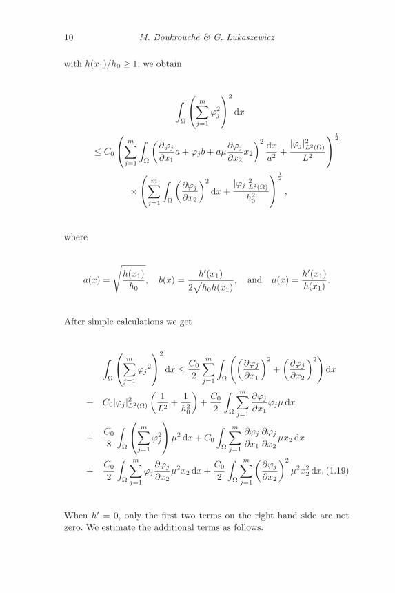
10 M. Boukrouche & G. �Lukaszewicz
with h(x1)/h0 ≥ 1, we obtain
∫Ω
⎛⎝ m∑j=1
ϕ2j
⎞⎠2
dx
≤ C0
⎛⎝ m∑j=1
∫Ω
(∂ϕj
∂x1a+ ϕjb+ aμ
∂ϕj
∂x2x2
)2 dxa2
+|ϕj |2L2(Ω)
L2
⎞⎠12
×⎛⎝ m∑
j=1
∫Ω
(∂ϕj
∂x2
)2
dx+|ϕj |2L2(Ω)
h20
⎞⎠12
,
where
a(x) =
√h(x1)h0
, b(x) =h′(x1)
2√h0h(x1)
, and μ(x) =h′(x1)h(x1)
.
After simple calculations we get
∫Ω
⎛⎝ m∑j=1
ϕj2
⎞⎠2
dx ≤ C0
2
m∑j=1
∫Ω
((∂ϕj
∂x1
)2
+(∂ϕj
∂x2
)2)
dx
+ C0|ϕj |2L2(Ω)
(1L2
+1h2
0
)+C0
2
∫Ω
m∑j=1
∂ϕj
∂x1ϕjμdx
+C0
8
∫Ω
⎛⎝ m∑j=1
ϕ2j
⎞⎠μ2 dx+ C0
∫Ω
m∑j=1
∂ϕj
∂x1
∂ϕj
∂x2μx2 dx
+C0
2
∫Ω
m∑j=1
ϕj∂ϕj
∂x2μ2x2 dx+
C0
2
∫Ω
m∑j=1
(∂ϕj
∂x2
)2
μ2x22 dx. (1.19)
When h′ = 0, only the first two terms on the right hand side are notzero. We estimate the additional terms as follows.
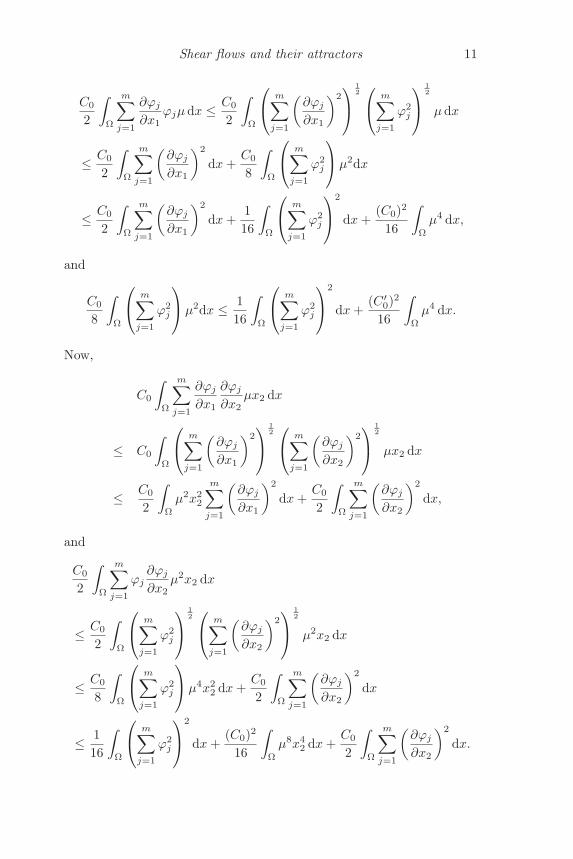
Shear flows and their attractors 11
C0
2
∫Ω
m∑j=1
∂ϕj
∂x1ϕjμdx ≤ C0
2
∫Ω
⎛⎝ m∑j=1
(∂ϕj
∂x1
)2⎞⎠
12⎛⎝ m∑
j=1
ϕ2j
⎞⎠12
μdx
≤ C0
2
∫Ω
m∑j=1
(∂ϕj
∂x1
)2
dx+C0
8
∫Ω
⎛⎝ m∑j=1
ϕ2j
⎞⎠μ2dx
≤ C0
2
∫Ω
m∑j=1
(∂ϕj
∂x1
)2
dx+116
∫Ω
⎛⎝ m∑j=1
ϕ2j
⎞⎠2
dx+(C0)2
16
∫Ω
μ4 dx,
and
C0
8
∫Ω
⎛⎝ m∑j=1
ϕ2j
⎞⎠μ2dx ≤ 116
∫Ω
⎛⎝ m∑j=1
ϕ2j
⎞⎠2
dx+(C ′
0)2
16
∫Ω
μ4 dx.
Now,
C0
∫Ω
m∑j=1
∂ϕj
∂x1
∂ϕj
∂x2μx2 dx
≤ C0
∫Ω
⎛⎝ m∑j=1
(∂ϕj
∂x1
)2⎞⎠
12⎛⎝ m∑
j=1
(∂ϕj
∂x2
)2⎞⎠
12
μx2 dx
≤ C0
2
∫Ω
μ2x22
m∑j=1
(∂ϕj
∂x1
)2
dx+C0
2
∫Ω
m∑j=1
(∂ϕj
∂x2
)2
dx,
and
C0
2
∫Ω
m∑j=1
ϕj∂ϕj
∂x2μ2x2 dx
≤ C0
2
∫Ω
⎛⎝ m∑j=1
ϕ2j
⎞⎠12⎛⎝ m∑
j=1
(∂ϕj
∂x2
)2⎞⎠
12
μ2x2 dx
≤ C0
8
∫Ω
⎛⎝ m∑j=1
ϕ2j
⎞⎠μ4x22 dx+
C0
2
∫Ω
m∑j=1
(∂ϕj
∂x2
)2
dx
≤ 116
∫Ω
⎛⎝ m∑j=1
ϕ2j
⎞⎠2
dx+(C0)2
16
∫Ω
μ8x42 dx+
C0
2
∫Ω
m∑j=1
(∂ϕj
∂x2
)2
dx.
12 M. Boukrouche & G. �Lukaszewicz
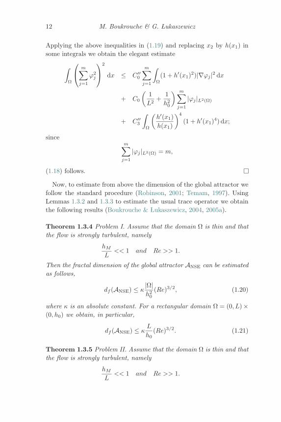
Applying the above inequalities in (1.19) and replacing x2 by h(x1) insome integrals we obtain the elegant estimate
∫Ω
⎛⎝ m∑j=1
ϕ2j
⎞⎠2
dx ≤ C ′′0
m∑j=1
∫Ω
(1 + h′(x1)2)|∇ϕj |2 dx
+ C0
(1L2
+1h2
0
) m∑j=1
|ϕj |L2(Ω)
+ C ′′3
∫Ω
(h′(x1)h(x1)
)4
(1 + h′(x1)4) dx;
sincem∑
j=1
|ϕj |L2(Ω) = m,
(1.18) follows.
Now, to estimate from above the dimension of the global attractor wefollow the standard procedure (Robinson, 2001; Temam, 1997). UsingLemmas 1.3.2 and 1.3.3 to estimate the usual trace operator we obtainthe following results (Boukrouche & �Lukaszewicz, 2004, 2005a).
Theorem 1.3.4 Problem I. Assume that the domain Ω is thin and thatthe flow is strongly turbulent, namely
hM
L<< 1 and Re >> 1.
Then the fractal dimension of the global attractor ANSE can be estimatedas follows,
df (ANSE) ≤ κ|Ω|h2
0
(Re)3/2, (1.20)
where κ is an absolute constant. For a rectangular domain Ω = (0, L) ×(0, h0) we obtain, in particular,
df (ANSE) ≤ κL
h0(Re)3/2. (1.21)
Theorem 1.3.5 Problem II. Assume that the domain Ω is thin and thatthe flow is strongly turbulent, namely
hM
L<< 1 and Re >> 1.
Shear flows and their attractors 13
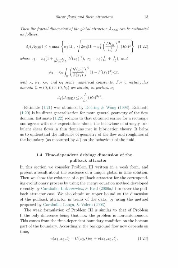
Then the fractal dimension of the global attractor ANSE can be estimatedas follows,
df (ANSE) ≤ κmax
{σ2|Ω| ,
√2σ3|Ω| + σ2
1
(LhM
h20
)2
(Re)3}
(1.22)
where σ1 = κ1(1 + max0≤x1≤L
|h′(x1)|2), σ2 = κ2( 1L2 + 1
h20), and
σ3 = κ3
∫Ω
(h′(x1)h(x1)
)4
(1 + h′(x1)4) dx,
with κ, κ1, κ2, and κ3 some numerical constants. For a rectangulardomain Ω = (0, L) × (0, h0) we obtain, in particular,
df (ANSE) ≤ κL
h0(Re)3/2.
Estimate (1.21) was obtained by Doering & Wang (1998). Estimate(1.20) is its direct generalization for more general geometry of the flowdomain. Estimate (1.22) reduces to that obtained earlier for a rectangleand agrees with our expectations about the behaviour of strongly tur-bulent shear flows in thin domains met in lubrication theory. It helpsus to understand the influence of geometry of the flow and roughness ofthe boundary (as measured by h′) on the behaviour of the fluid.
1.4 Time-dependent driving: dimension of thepullback attractor
In this section we consider Problem III written in a weak form, andpresent a result about the existence of a unique global in time solution.Then we show the existence of a pullback attractor for the correspond-ing evolutionary process by using the energy equation method developedrecently by Caraballo, �Lukaszewicz, & Real (2006a,b) to cover the pull-back attractor case. We also obtain an upper bound on the dimensionof the pullback attractor in terms of the data, by using the methodproposed by Caraballo, Langa, & Valero (2003).
The weak formulation of Problem III is similar to that of ProblemI, the only difference being that now the problem is non-autonomous.This comes from the time-dependent boundary condition on the bottompart of the boundary. Accordingly, the background flow now depends ontime,
u(x1, x2, t) = U(x2, t)e1 + v(x1, x2, t), (1.23)
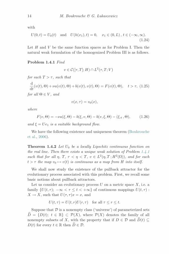
14 M. Boukrouche & G. �Lukaszewicz
with
U(0, t) = U0(t) and U(h(x1), t) = 0, x1 ∈ (0, L) , t ∈ (−∞,∞).(1.24)
Let H and V be the same function spaces as for Problem I. Then thenatural weak formulation of the homogenized Problem III is as follows.
Problem 1.4.1 Find
v ∈ C([τ, T ];H) ∩ L2(τ, T ;V )
for each T > τ , such that
ddt
(v(t),Θ) + νa(v(t),Θ) + b(v(t), v(t),Θ) = F (v(t),Θ), t > τ, (1.25)
for all Θ ∈ V , and
v(x, τ) = v0(x),
where
F (v,Θ) = −νa(ξ,Θ) − b(ξ, v,Θ) − b(v, ξ,Θ) − (ξ,t ,Θ), (1.26)
and ξ = Ue1 is a suitable background flow.
We have the following existence and uniqueness theorem (Boukroucheet al., 2006).
Theorem 1.4.2 Let U0 be a locally Lipschitz continuous function onthe real line. Then there exists a unique weak solution of Problem 1.4.1such that for all η, T , τ < η < T , v ∈ L2(η, T ;H2(Ω)), and for eacht > τ the map v0 �→ v(t) is continuous as a map from H into itself.
We shall now study the existence of the pullback attractor for theevolutionary process associated with this problem. First, we recall somebasic notions about pullback attractors.
Let us consider an evolutionary process U on a metric space X, i.e. afamily {U(t, τ); −∞ < τ ≤ t < +∞} of continuous mappings U(t, τ) :X → X, such that U(τ, τ)x = x, and
U(t, τ) = U(t, r)U(r, τ) for all τ ≤ r ≤ t.
Suppose that D is a nonempty class (‘universe’) of parameterized setsD = {D(t); t ∈ R} ⊂ P(X), where P(X) denotes the family of allnonempty subsets of X, with the property that if D ∈ D and D(t) ⊆D(t) for every t ∈ R then D ∈ D.
Shear flows and their attractors 15
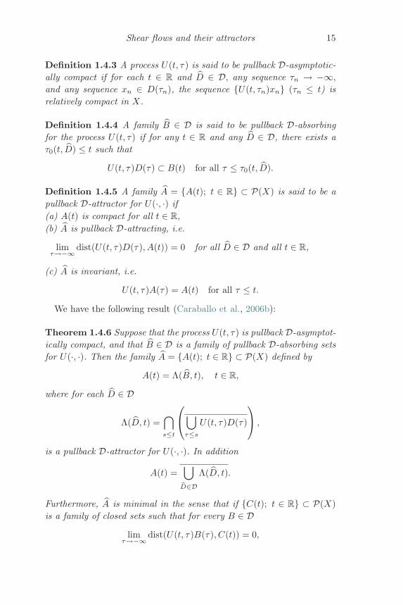
Definition 1.4.3 A process U(t, τ) is said to be pullback D-asymptotic-ally compact if for each t ∈ R and D ∈ D, any sequence τn → −∞,
and any sequence xn ∈ D(τn), the sequence {U(t, τn)xn} (τn ≤ t) isrelatively compact in X.
Definition 1.4.4 A family B ∈ D is said to be pullback D-absorbingfor the process U(t, τ) if for any t ∈ R and any D ∈ D, there exists aτ0(t, D) ≤ t such that
U(t, τ)D(τ) ⊂ B(t) for all τ ≤ τ0(t, D).
Definition 1.4.5 A family A = {A(t); t ∈ R} ⊂ P(X) is said to be apullback D-attractor for U(·, ·) if(a) A(t) is compact for all t ∈ R,(b) A is pullback D-attracting, i.e.
limτ→−∞ dist(U(t, τ)D(τ), A(t)) = 0 for all D ∈ D and all t ∈ R,
(c) A is invariant, i.e.
U(t, τ)A(τ) = A(t) for all τ ≤ t.
We have the following result (Caraballo et al., 2006b):
Theorem 1.4.6 Suppose that the process U(t, τ) is pullback D-asymptot-ically compact, and that B ∈ D is a family of pullback D-absorbing setsfor U(·, ·). Then the family A = {A(t); t ∈ R} ⊂ P(X) defined by
A(t) = Λ(B, t), t ∈ R,
where for each D ∈ D
Λ(D, t) =⋂s≤t
⎛⎝⋃τ≤s
U(t, τ)D(τ)
⎞⎠ ,
is a pullback D-attractor for U(·, ·). In addition
A(t) =⋃
D∈DΛ(D, t).
Furthermore, A is minimal in the sense that if {C(t); t ∈ R} ⊂ P(X)is a family of closed sets such that for every B ∈ D
limτ→−∞ dist(U(t, τ)B(τ), C(t)) = 0,
16 M. Boukrouche & G. �Lukaszewicz
then A(t) ⊆ C(t).Now, we come back to the context of Problem 1.4.1. For t ≥ τ let us
define the map U(t, τ) in H by
U(t, τ)v0 = v(t; τ, v0), t ≥ τ, v0 ∈ H, (1.27)
where v(t; τ, v0) is the solution of Problem 1.4.1. From the uniquenessof solutions to this problem, one immediately obtains
U(t, τ)v0 = U(t, r)(U(r, τ)v0), for all τ ≤ r ≤ t, v0 ∈ H.
From Theorem 1.4.2 it follows that for all t ≥ τ, the process mappingU(t, τ) : H → H, defined by (1.27), is continuous. Consequently, thefamily {U(t, τ), τ ≤ t} defined by (1.27) is a process in H.
We define the universe of the parameterized families of sets as follows:for σ = νλ1 and |D(t)|+ = sup{|y| : y ∈ D(t)}, let
Dσ = {D : R → P(H); limt→−∞ eσt(|D(t)|+)2 = 0}.
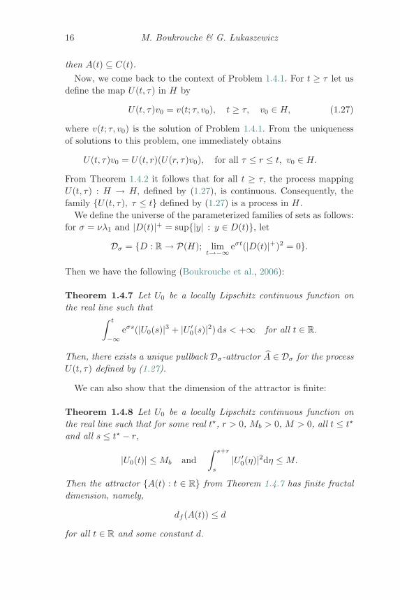
Then we have the following (Boukrouche et al., 2006):
Theorem 1.4.7 Let U0 be a locally Lipschitz continuous function onthe real line such that∫ t
−∞eσs(|U0(s)|3 + |U ′
0(s)|2) ds < +∞ for all t ∈ R.
Then, there exists a unique pullback Dσ-attractor A ∈ Dσ for the processU(t, τ) defined by (1.27).
We can also show that the dimension of the attractor is finite:
Theorem 1.4.8 Let U0 be a locally Lipschitz continuous function onthe real line such that for some real t�, r > 0, Mb > 0, M > 0, all t ≤ t�
and all s ≤ t� − r,
|U0(t)| ≤Mb and∫ s+r
s
|U ′0(η)|2dη ≤M.
Then the attractor {A(t) : t ∈ R} from Theorem 1.4.7 has finite fractaldimension, namely,
df (A(t)) ≤ d
for all t ∈ R and some constant d.
Shear flows and their attractors 17
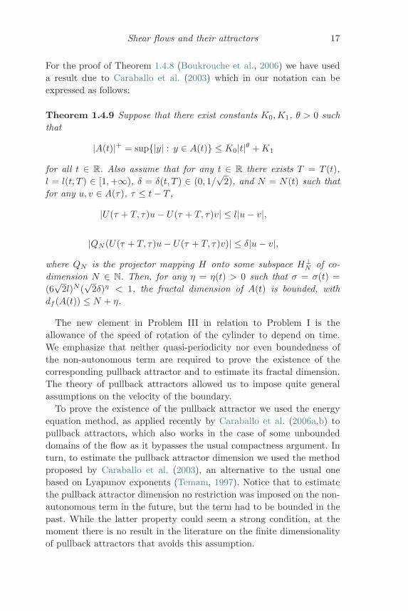
For the proof of Theorem 1.4.8 (Boukrouche et al., 2006) we have useda result due to Caraballo et al. (2003) which in our notation can beexpressed as follows:
Theorem 1.4.9 Suppose that there exist constants K0,K1, θ > 0 suchthat
|A(t)|+ = sup{|y| : y ∈ A(t)} ≤ K0|t|θ +K1
for all t ∈ R. Also assume that for any t ∈ R there exists T = T (t),l = l(t, T ) ∈ [1,+∞), δ = δ(t, T ) ∈ (0, 1/
√2), and N = N(t) such that
for any u, v ∈ A(τ), τ ≤ t− T ,
|U(τ + T, τ)u− U(τ + T, τ)v| ≤ l|u− v|,
|QN (U(τ + T, τ)u− U(τ + T, τ)v)| ≤ δ|u− v|,
where QN is the projector mapping H onto some subspace H⊥N of co-
dimension N ∈ N. Then, for any η = η(t) > 0 such that σ = σ(t) =(6√
2l)N (√
2δ)η < 1, the fractal dimension of A(t) is bounded, withdf (A(t)) ≤ N + η.
The new element in Problem III in relation to Problem I is theallowance of the speed of rotation of the cylinder to depend on time.We emphasize that neither quasi-periodicity nor even boundedness ofthe non-autonomous term are required to prove the existence of thecorresponding pullback attractor and to estimate its fractal dimension.The theory of pullback attractors allowed us to impose quite generalassumptions on the velocity of the boundary.
To prove the existence of the pullback attractor we used the energyequation method, as applied recently by Caraballo et al. (2006a,b) topullback attractors, which also works in the case of some unboundeddomains of the flow as it bypasses the usual compactness argument. Inturn, to estimate the pullback attractor dimension we used the methodproposed by Caraballo et al. (2003), an alternative to the usual onebased on Lyapunov exponents (Temam, 1997). Notice that to estimatethe pullback attractor dimension no restriction was imposed on the non-autonomous term in the future, but the term had to be bounded in thepast. While the latter property could seem a strong condition, at themoment there is no result in the literature on the finite dimensionalityof pullback attractors that avoids this assumption.
18 M. Boukrouche & G. �Lukaszewicz
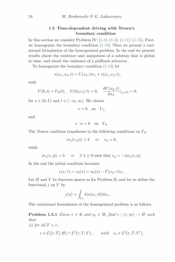
1.5 Time-dependent driving with Tresca’sboundary condition
In this section we consider Problem IV: (1.1)–(1.3), (1.11)–(1.13). First,we homogenize the boundary condition (1.13). Then we present a vari-ational formulation of the homogenized problem. In the end we presentresults about the existence and uniqueness of a solution that is globalin time, and about the existence of a pullback attractor.
To homogenize the boundary condition (1.13) let
u(x1, x2, t) = U(x2, t)e1 + v(x1, x2, t),
with
U(0, t) = U0(t), U(h(x1), t) = 0,∂U(x2, t)∂x2
|x2=0 = 0,
for x ∈ (0, L) and t ∈ (−∞,∞). We obtain
v = 0 on Γ1,
and
v · n = 0 on Γ0.
The Tresca condition transforms to the following conditions on Γ0:
|ση(v, p)| < k ⇒ vη = 0,
while
|ση(v, p)| = k ⇒ ∃ λ ≥ 0 such that vη = −λση(v, p).
In the end the initial condition becomes
v(x, τ) = v0(x) = u0(x) − U(x2, τ)e1.
Let H and V be function spaces as for Problem II, and let us define thefunctional j on V by
j(u) =∫
Γ0
k|u(x1, 0)|dx1.
The variational formulation of the homogenized problem is as follows.
Problem 1.5.1 Given τ ∈ R and v0 ∈ H, find v : (τ,∞) → H suchthat:(i) for all T > τ ,
v ∈ C([τ, T ];H) ∩ L2(τ, T ;V ), with vt ∈ L2(τ, T ;V ′),
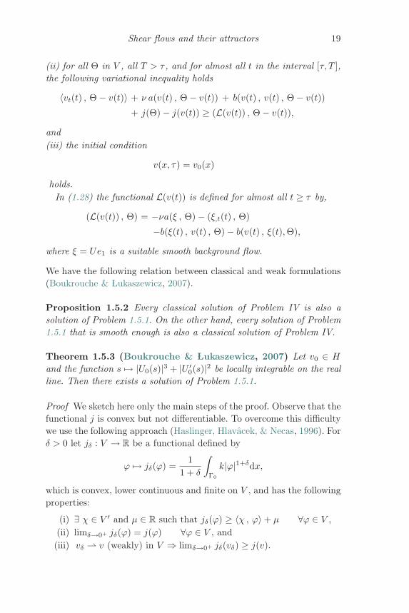
Shear flows and their attractors 19
(ii) for all Θ in V , all T > τ , and for almost all t in the interval [τ, T ],the following variational inequality holds
〈vt(t) , Θ − v(t)〉 + ν a(v(t) , Θ − v(t)) + b(v(t) , v(t) , Θ − v(t))
+ j(Θ) − j(v(t)) ≥ (L(v(t)) , Θ − v(t)),
and(iii) the initial condition
v(x, τ) = v0(x)
holds.In (1.28) the functional L(v(t)) is defined for almost all t ≥ τ by,
(L(v(t)) , Θ) = −νa(ξ , Θ) − (ξ,t(t) , Θ)
−b(ξ(t) , v(t) , Θ) − b(v(t) , ξ(t),Θ),
where ξ = Ue1 is a suitable smooth background flow.
We have the following relation between classical and weak formulations(Boukrouche & �Lukaszewicz, 2007).
Proposition 1.5.2 Every classical solution of Problem IV is also asolution of Problem 1.5.1. On the other hand, every solution of Problem1.5.1 that is smooth enough is also a classical solution of Problem IV.
Theorem 1.5.3 (Boukrouche & �Lukaszewicz, 2007) Let v0 ∈ H
and the function s �→ |U0(s)|3 + |U ′0(s)|2 be locally integrable on the real
line. Then there exists a solution of Problem 1.5.1.
Proof We sketch here only the main steps of the proof. Observe that thefunctional j is convex but not differentiable. To overcome this difficultywe use the following approach (Haslinger, Hlavacek, & Necas, 1996). Forδ > 0 let jδ : V → R be a functional defined by
ϕ �→ jδ(ϕ) =1
1 + δ
∫Γ0
k|ϕ|1+δdx,
which is convex, lower continuous and finite on V , and has the followingproperties:
(i) ∃ χ ∈ V ′ and μ ∈ R such that jδ(ϕ) ≥ 〈χ , ϕ〉 + μ ∀ϕ ∈ V ,(ii) limδ→0+ jδ(ϕ) = j(ϕ) ∀ϕ ∈ V , and
(iii) vδ ⇀ v (weakly) in V ⇒ limδ→0+ jδ(vδ) ≥ j(v).
20 M. Boukrouche & G. �Lukaszewicz
The functional jδ is Gateaux differentiable in V , with
(j′δ(v) , Θ) =∫
Γ0
k|v|δ−1 vΘ dx ∀ Θ ∈ V.
We consider the following equation(dvδ
dt, Θ
)+ νa(vδ(t) , Θ) + b(vδ(t) , vδ(t),Θ) + (j′δ(vδ) , Θ)
= −νa(ξ(t) , Θ) − (ξ,t , Θ) − b(ξ(t) , vδ(t),Θ) − b(vδ(t) , ξ(t) ,Θ),
with initial condition
vδ(τ) = v0,
establish an a priori estimate for vδ for δ > 0, and then show that thelimit function v is a solution to Problem 1.5.1.
Moreover, the solution is unique and depends continuously on theinitial data, namely, we have the following:
Theorem 1.5.4 Under the hypotheses of Theorem 1.5.3, the solutionv of Problem 1.5.1 is unique and the map v(τ) → v(t), for t > τ , iscontinuous from H into itself.
Now we shall study existence of the pullback attractor using a methodbased on the concept of the Kuratowski measure of non-compactness ofa bounded set, developed by Song & Wu (2007). This method is veryuseful when one deals with variational inequalities as it overcomes obsta-cles coming from the usual methods. One needs neither compactnessof the dynamics which results from the second energy inequality norasymptotic compactness, see Boukrouche et al. (2006), Caraballo et al.(2006a,b), or Temam (1997), which results from the energy equation.In the case of variational inequalities it is sometimes very difficult toobtain the second energy inequality due to the presence of boundaryfunctionals, on the other hand, we do not have any energy equation.
We now recast the theory of Song & Wu (2007) in the language ofevolutionary processes, and then apply it to our problem. Recall thatthe Kuratowski measure of non-compactness (Kuratowski, 1930) of abounded subset B of H, α(B), is defined as
α(B) = inf{δ : B admits a finite cover by sets of diameter ≤ δ}.
Shear flows and their attractors 21
Definition 1.5.5 The process U(t, τ) is said to be pullback ω-limitcompact if for any B ∈ B(H), for t ∈ R,
limτ→∞α
⎛⎝ ⋃s≤t−τ
U(t, s)B
⎞⎠ = 0.
In fact U is pullback ω-limit compact if and only if it is pullbackD-asymptotically compact in the sense of Definition 1.4.3, where D istaken to be the collection of all time-independent bounded sets (see, forexample, Kloeden & Langa, 2007).
Definition 1.5.6 Let H be a Banach space. The process U is said to benorm-to-weak continuous on H if for all (t, s, x) ∈ R×R×H with t ≥ s
and for every sequence (xn) ∈ H,
xn → x strongly in H =⇒ U(t, s)xn ⇀ U(t, s)x weakly in H.
Theorem 1.5.7 Let H be a Banach space, and U a process on H. If Uis norm-to-weak continuous and possesses a uniformly absorbing set B0,then U possesses a pullback attractor A = {A(t)}t∈R, with
A(t) = Λ(B0, t) ∀ t ∈ R,
if and only if it is pullback ω-limit compact.
We now state the main theorem from Song & Wu (2007). Theterminology “flattening property” was coined by Kloeden & Langa(2007).
Theorem 1.5.8 (cf. Song & Wu, 2007) Let H be a Banach space. Ifthe process U has the pullback flattening property, i.e. if for any t ∈ R,a bounded subset B of H, and ε > 0, there exists an s0(t, B, ε) and afinite-dimensional subspace E of H such that for some bounded projectorP : H → E,
P
⎛⎝ ⋃s≤s0
U(t, s)B
⎞⎠ is bounded
and ∣∣∣∣∣(I − P )
⎛⎝ ⋃s≤s0
U(t, s)B
⎞⎠∣∣∣∣∣ ≤ ε,
then U is pullback ω-limit compact.
22 M. Boukrouche & G. �Lukaszewicz
Now let U be the evolutionary process associated with Problem 1.5.1.
Lemma 1.5.9 Let
suph∈R
∫ h+1
h
F (s) ds < R(F ) <∞, (1.28)
σ > 0 and t ≥ τ . Then for every ε > 0 there exists δ = δ(ε) > 0 suchthat ∫ t
τ
e−σ(t−s)F (s) ds ≤ ε
2+
e−σδ
1 − e−σR(F ).
Proof Let δ be such that∫ t
t−δF (s)ds ≤ ε
2 , τ < δ < t. Then, by (1.28),∫ t
τ
e−σ(t−s)F (s)ds ≤ ε
2+
∞∑k=1
∫ t−(δ+k)
t−(δ+k+1)
e−σ(t−s)F (s)ds
≤ ε
2+
e−σδ
1 − e−σR(F ).
Let F (s) = |U0(s)|3 + |U ′0(s)|2, cf. Theorem 1.5.3. Then we have
Lemma 1.5.10 Let the initial condition v0 in Problem 1.5.1 belong toa ball B(0, ρ) in H. Suppose that (1.28) holds. Then the solution v ofProblem 1.5.1 satisfies
suph≥τ
∫ h+1
h
|∇v(s)|2ds ≤ 2ν{ρ2 + (1 +
e−σδ
1 − e−σ)R(F )}. (1.29)
Proof Taking Θ = 0 in (1.28) we obtain,
12
ddt
|v(t)|2 +ν
2|∇v(t)|2 ≤ F (t) (1.30)
and, in consequence,
12
ddt
|v(t)|2 +σ
2|v(t)|2 ≤ F (t), (1.31)
with σ = νλ1. By Gronwall’s inequality and Lemma 1.5.9 with ε = ρ2
we conclude from the last inequality that for t ≥ τ ,
|v(t)|2 ≤ 2ρ2 +2e−σδ
1 − e−σR(F ). (1.32)
Shear flows and their attractors 23
Integrating (1.30) we obtain the first energy estimate: for τ ≤ η ≤ t,
|v(t)|2 + ν
∫ t
η
|∇v(s)|2ds ≤ 2∫ t
η
F (s)ds+ |v(η)|2.
Using this estimate and (1.32) we obtain (1.29).
Theorem 1.5.11 Let v0 ∈ H and U0 be such that (1.28) holds, withF (s) = |U0(s)|3 + |U ′
0(s)|2. Then there exists a pullback attractor A inthe sense of Theorem 1.5.7 for the evolutionary process U .
Proof From (1.31), (1.32), the Gronwall inequality, and Lemma 1.5.9we obtain
|U(s+ t, t)v0|2 ≤ e−σs|v0|2 + ε+2e−σδ
1 − e−σR(F ).
For v0 in B(0, ρ) and s large enough, U(s + t, t)v0 ∈ B(0, ρ0), whereρ0 depends only on ε, ρ, and R(F ), which means that there exists auniformly absorbing ball in H.
From Theorem 1.5.4 it follows that the evolutionary process U isstrongly continuous in H, whence, in particular, it is norm-to-weakcontinuous on H.
Thus, according to Theorem 1.5.7 and Theorem 1.5.8, to finish theproof we have to prove that U has the pullback flattening property.
Let A be the Stokes operator in H. Since A−1 is continuous and com-pact in H, there exists a sequence {λj}∞j=1 such that 0 < λ1 ≤ λ2 ≤ . . . ≤λj ≤ . . . with limj→+∞ λj = ∞, and a family of elements {ϕj}∞j=1 ofD(A), which are orthonormal in H such that Aϕj = λjϕj .
We define the m-dimensional subspace Vm, of V , and the orthogonalprojection operator Pm : V → Vm by Vm = span{ϕ1, . . . , ϕm} andPmv =
∑mj=1(v , ϕj)ϕj . For v ∈ D(A) ⊂ V we can decompose v as
v = Pmv + (I − Pm)v = Pmv + v2.
Set Θ = v1(t) in (1.28) to get
12
ddt
|v2(t)|2 + ν|∇v2(t)|2 ≤ j(v1(t)) − j(v(t)) − b(v(t) , v(t) , v2(t))
+ (L(v(t)) , v2(t)).
From the continuity of the trace operator we have
j(v1(t)) − j(v(t)) ≤ j(v2(t)) ≤ C +ν
4‖v2(t)‖2.
24 M. Boukrouche & G. �Lukaszewicz
Using the anisotropic Ladyzhenskaya inequality ‖v‖L4(Ω) ≤ C|v| 12 |∇v| 12(where C = C(Ω)) we easily arrive at
ddt
|v2(t)|2 + ν|∇v2(t)|2 ≤ C2(1 + F (t) + |∇v(t)|2).
andddt
|v2(t)|2 + νλm+1|v2(t)|2 ≤ C2(1 + F (t) + |∇v(t)|2).
Now, let ε > 0 be given. Using Lemmas 1.5.9 and 1.5.10, and takingm large enough, we obtain
|(I − Pm)U(s+ t, t)v0|2 ≤ ε
uniformly in t, for v0 ∈ B(0, ρ) and all s ≥ s0(ρ, ε) large enough. Thisends the proof of the theorem.
Acknowledgements
This research was supported by the Polish Government Grant MEiN 1P303A 017 30 and Project FP6 EU SPADE2.
ReferencesBoukrouche, M. & �Lukaszewicz, G. (2004) An upper bound on the attractor
dimension of a 2D turbulent shear flow in lubrication theory. NonlinearAnalysis 59, 1077–1089.
Boukrouche, M. & �Lukaszewicz, G. (2005a) An upper bound on the attractordimension of a 2D turbulent shear flow with a free boundary condition,in Regularity and other Aspects of the Navier–Stokes Equations, BanachCenter Publications 70, 61–72, Institute of Mathematics, Polish Academyof Science, Warszawa.
Boukrouche, M. & �Lukaszewicz, G. (2005b) Attractor dimension estimate forplane shear flow of micropolar fluid with free boundary. MathematicalMethods in the Applied Sciences 28, 1673–1694.
Boukrouche, M. & �Lukaszewicz, G. (2007) On the existence of pullback attrac-tor for a two-dimensional shear flow with Tresca’s boundary condition, inParabolic and Navier–Stokes Equations. Banach Center Publications 81,81–93, Institute of Mathematics, Polish Academy of Science, Warszawa.
Boukrouche, M., �Lukaszewicz, G., & Real, J. (2006) On pullback attractorsfor a class of two-dimensional turbulent shear flows. International Journalof Engineering Science 44, 830–844.
Caraballo, T., Langa, J.A., & Valero, J. (2003) The dimension of attractors ofnon-autonomous partial differential equations. ANZIAM J. 45, 207–222.
Caraballo, T., �Lukaszewicz, G., & Real, J. (2006a) Pullback attractors forasymptotically compact non-autonomous dynamical systems. NonlinearAnalysis, TMA 64, 484–498.
Shear flows and their attractors 25
Caraballo, T., �Lukaszewicz, G., & Real, J. (2006b) Pullback attractors for non-autonomous 2D-Navier–Stokes equations in some unbounded domains.C. R. Acad. Sci. Paris, Ser. I 342, 263–268.
Chepyzhov, V.V. & Vishik, M.I. (2002) Attractors for equations of mathemat-ical physics. Providence, RI.
Doering, C.R. & Constantin, P. (1991) Energy dissipation in shear driventurbulence. Phys. Rev. Lett. 69, 1648–1651.
Doering, C.R. & Gibbon, J.D. (1995) Applied Analysis of the Navier–StokesEquations. Cambridge University Press, Cambridge.
Doering, C.R. & Wang, X. (1998) Attractor dimension estimates for two-dimensional shear flows. Physica D 123, 206–222.
Duvaut, G. & Lions, J.L. (1972) Les inequations en mecanique et en physique.Dunod, Paris.
Falconer, K. (1990) Fractal Geometry. Wiley, Chichester.Foias, C., Manley, O., Rosa, R., & Temam, R. (2001) Navier–Stokes Equations
and Turbulence. Cambridge University Press, Cambridge.Haslinger, J., Hlavacek, I., & Necas, J. (1996) Numerical Methods for
unilateral problems in solid mechanics, in Ciarlet, P.G. & Lions, J.L.(eds.), Handbook of Numerical Analysis, Vol IV, 313–485, North Holland,Amsterdam.
Kloeden, P.K. & Langa, J.A. (2007) Flattening, squeezing, and the existenceof random attractors. Proc. Roy. Soc. London A 463, 163–181.
Kuratowski, K. (1930) Sur les espaces complets. Fund. Math. 15, 301–309.�Lukaszewicz, G. & Sadowski, W. (2004) Uniform attractor for 2D magneto-
micropolar fluid flow in some unbounded domains. Z. Angew. Math. Phys.55, 1–11.
Miranville, A. & Wang, X. (1997) Attractor for non-autonomous nonhomoge-neous Navier–Stokes equations. Nonlinearity 10, 1047–1061.
Miranville, A. & Ziane, M. (1997) On the dimension of the attractor for theBenard problem with free surfaces. Russian J. Math. Phys. 5, 489–502.
Moise, I., Rosa, R., & Wang, X. (2004) Attractors for non-compact non-autonomous systems via energy equations. Discrete and ContinuousDynamical Systems 10, 473–496.
Mucha, P. & Sadowski, W. (2005) Long time behaviour of a flow in infinitepipe conforming to slip boundary conditions. Mathematical Methods inthe Applied Sciences 28, 1867–1880.
Robinson, J.C. (2001) Infinite-Dimensional Dynamical Systems. CambridgeUniversity Press, Cambridge.
Song, H. & Wu, H. (2007) Pullback attractors of non-autonomous reaction-diffusion equations. J.Math. Anal. Appl. 325, 1200–1215.
Temam, R. (1997) Infinite Dimensional Dynamical Systems in Mechanics andPhysics. Second Edition, Springer-Verlag, New York.
Temam, R. & Ziane, M. (1998) Navier–Stokes equations in three-dimensionalthin domains with various boundary conditions. Adv. in DifferentialEquations 1, 1–21.
Ziane, M. (1997) Optimal bounds on the dimension of the attractor of theNavier–Stokes equations. Physica D 105, 1–19.
Ziane, M. (1998) On the 2D-Navier–Stokes equations with the free boundarycondition. Appl. Math. and Optimization 38, 1–19.
2
Mathematical results concerning unsteadyflows of chemically reacting incompressible
fluidsMiroslav Bulıcek
Charles University, Faculty of Mathematics and Physics,Mathematical Institute, Sokolovska 83, 186 75 Prague 8. Czech Republic.
Josef MalekCharles University, Faculty of Mathematics and Physics,
Mathematical Institute, Sokolovska 83, 186 75 Prague 8. Czech [email protected]
Kumbakonam R. RajagopalDepartment of Mechanical Engineering, Texas A&M University,
College Station, TX 77843. [email protected]
Abstract
We investigate the mathematical properties of unsteady three-dimensional internal flows of chemically reacting incompressible shear-thinning (or shear-thickening) fluids. Assuming that we have Navier’sslip at the impermeable boundary we establish the long-time existenceof a weak solution when the data are large.
2.1 Introduction
Even though 150 years have elapsed since Darcy (1856) published hiscelebrated study, the equation he introduced (or minor modifications ofit) remains as the main model to describe the flow of fluids throughporous media due to a pressure gradient. While the equation that Darcyprovided in his study is referred to as a “law” it is merely an approx-imation, and a very simple one at that, for the flow of a fluid throughporous media. The original equation due to Darcy can be shown to bean approximation of the equations governing the flow of a fluid througha porous solid within the context of the theory of mixtures by appeal-ing to numerous assumptions (Atkin & Craine, 1976a,b; Bowen, 1975;
Published in Partial Differential Equations and Fluid Mechanics, edited byJames C. Robinson and Jose L. Rodrigo. c© Cambridge University Press 2009.
Chemically reacting incompressible fluids 27
Green & Naghdi, 1969; Adkins, 1963a,b). Hassanizadeh (1986) and Gray(1983) have also shown that Darcy’s equation can be obtained usingan averaging technique, but not within the context of mixtures. Toobtain Darcy’s equation within the context of the theory of mixtures, oneignores the balance of linear momentum for the solid (which is assumedto be rigid and thus the stress is whatever it needs to be in order forthe flow to take place), assumes that the only interaction between thefluid and the solid is the frictional resistance at the pores of the solid,and that this resistance is proportional to the difference in the velocitybetween the fluid and solid. The frictional effects within the fluid andthus the dissipation within the fluid are ignored. If the frictional resis-tance at the pore, between the solid and the fluid, is not assumed to beproportional to the difference in velocity between the fluid and the solid,but depends, in another way, in a nonlinear manner on the difference,one obtains the Darcy–Forchheimer equation (see Forchheimer, 1901).If the viscosity of the fluid is not neglected, i.e. the viscous dissipationin the fluid is not ignored, and if it is assumed that it is like that in theclassical Navier–Stokes fluid, then one obtains the equation developedby Brinkman (1947a,b) (see also Rajagopal, 2007).
An interesting counterpart presents itself when we consider a complexfluid such as blood which is maintained in a state of delicate balanceby virtue of a myriad of chemical reactions that take place, some thatcause the blood to coagulate, others that cause lysis, etc. In fact, eventhe development of a simple model for blood requires dozens of equa-tions and these govern the biochemical reactions that have to be coupledto the balance equations (Anand, Rajagopal, & Rajagopal, 2003, 2005).As blood involves constituents that can be modelled by the Navier–Stokes model (for the plasma for instance) or a purely elastic model (sayfor platelets) and others that are viscoelastic solids (cells) or viscoelas-tic fluids, one would have a system of equations that would be totallyintractable. Thus, it is absolutely necessary to simplify the model whilecapturing the quintessential feature of the mechanical response charac-teristics. Instead of keeping track of all the constituents of blood, eventhough it might be an oversimplification, one could consider blood asa homogeneous fluid whose properties change due to a chemical statevariable, which we shall refer to as the concentration c, which is a con-sequence of all chemical reactions that take place. Thus, in essence, weare replacing a plethora of chemical reactions by a single equation thathas the same effect, on average, as the system of reactions that actuallyoccur.
28 M. Bulıcek, J. Malek, & K.R. Rajagopal
It is then possible to model the flow of blood through a coupled systemof equations: the balance of mass, linear and angular momentum for thehomogeneous single fluid, and an advection-diffusion equation for thechemical state variable c, the concentration. It is also possible to thinkof blood as a single homogeneous fluid that is co-occupying the flowdomain with another fluid that is capable of reacting with the homo-geneous fluid and thereby changing its properties. This reacting fluidis carried along by the flowing fluid, and in the spirit of the develop-ment of Darcy’s equation, we can choose to ignore the balance equationfor the reacting fluid (similar to ignoring the balance equations for theporous solid). As the second fluid moves with the same velocity as thecarrier, we do not have an interactive force like the “drag force” thatis a consequence of the relative velocity between the two fluids, actingon the fluids. Bridges & Rajagopal (2006) associate the concentrationwith the ratio of the density of the reactant to the sum of the density ofthe reactant and the homogeneous fluid. While a concentration definedin such a manner tends to zero when the density of the second fluidtends to zero, it cannot tend to unity as the density of the carrier fluid(which they assume to be incompressible) is not zero and the density ofthe reacting fluid is finite. Though Bridges & Rajagopal (2006) motivatethe concentration through such a ratio, as far as their study is concernedthe concentration c is merely treated as a variable that can change (onecould view it as an internal variable with a clear physical underpinning,namely the concentration of a second fluid that is undergoing a reaction).
As blood is a multi-constituent material, with the constituents dis-tributed in the vessel in an inhomogeneous manner, it would be moreappropriate to approximate it as a single constituent fluid that is inho-mogeneous; that is, the homogenization of the multi-constituent bodyleads to an inhomogeneous body. It is important to recognize that whilereferring to the “homogenization” of the body we are referring to anaveraging procedure of the multi-constituents, while when describing thebody as inhomogeneous we are referring to the fact that the averagedbody has properties that change from one material point to another. Itis important to keep this distinction in mind. In the study that is beingcarried out, we are able to capture this inhomogeneity by allowing thematerial properties to change due to the presence of chemical reactionswhich arise from the concentration of reactants that are carried alongby the homogeneous fluid (see the more detailed explanation that fol-lows). It is also important to recognize that if the properties of a fluidvary in a particular configuration of the fluid this does not imply that
Chemically reacting incompressible fluids 29
the fluid is inhomogeneous as one merely needs a configuration (someconfiguration in which the body can be placed) in which the propertiesof a body are the same for the body to be homogeneous. A body is saidto be homogeneous if there exists a configuration in which the propertiesof the body are the same at every point in the configuration. Considera fluid with shear-rate-dependent viscosity. At rest, corresponding tozero shear rate, the viscosity of the fluid is the zero-shear-rate viscos-ity. However, during a flow in which the shear rate varies in the body,the viscosity will not be the same everywhere. We cannot conclude fromthe viscosity not being the same everywhere that the body is inhomoge-neous. There is a configuration, namely that corresponding to the stateof rest where the properties are the same, and hence the body is homoge-neous. The monograph by Truesdell (1991) contains a general discussionof homogeneity and Anand & Rajagopal (2004) give examples of flowsof inhomogeneous fluids where material properties other than just thedensity being non-constant are considered. There are numerous studiesconcerning fluids with non-constant density, going back to the seminalwork of Lord Rayleigh (1883), and the books by Yih (1965, 1980) aredevoted to the study of the flows of such fluids.
Bridges & Rajagopal (2006) studied the pulsating flow of a chemicallyreacting incompressible fluid in terms of the balance equations for ahomogenized fluid (as explained above, the equation considered there isan averaged equation for a single “average” constituent, the averagedsingle constituent not being necessarily a homogeneous body in thatits properties are the same at every material point) and a diffusion-convection equation for the concentration c.
If the fluid (reactant) that is being carried along and the carrier fluid(which is the fluid obtained by “homogenizing” the multi-constituentfluid such as blood) are of comparable density, then assigning the notionof the ratio of the density of the reactant to the total density would notbe appropriate as the balance of linear momentum for the fluid that iscarried, whose properties are changing due to the reaction, cannot beexpressed merely in terms of its density as the inertial term would havea contribution due to the density of the fluid that is also carried along.We are primarily interested in the fluid that is carried along and reactingwith our fluid of interest having associated with it a much smaller andin fact ignorable density. Thus, as mentioned earlier, in the work ofBridges & Rajagopal (2006) the concentration has to be interpreted inthe sense of a variable that is a measure of the reaction rather thana ratio of densities. This point is not made clear in their work though
30 M. Bulıcek, J. Malek, & K.R. Rajagopal
they do mention that c could be an internal variable, which we refer toas a chemical state variable. Here, we shall choose to think of c as achemical state variable rather than the ratio of densities, and we shallsuppose that the reactant that is carried is not of comparable density tothe fluid of interest.
While it would be preferable to study the problem of multi-constituentmaterials such as blood within the context of mixture theory such anapproach is not without serious difficulties. Not only is it necessary tokeep track of all the individual constituents and provide constitutiverelations for them, as well as model all the interactions between theconstituents, we have a far deeper problem, that of providing boundaryconditions for each of the constituents. Usually, one is able to ascertainonly the boundary conditions for the mixture as a whole and this is abasic problem that is inherent to mixture theory (see Rajagopal & Tao(1995) for a detailed discussion of the same topic).
It is well established that blood in large blood vessels like the aortabehaves essentially as a Navier–Stokes fluid while in narrower blood ves-sels it can be approximated as a single-constituent fluid that shear thins.In fact, the generalized viscosity associated with such a shear-thinningfluid can change by a factor of forty (Yeleswarapu, 1996; Yeleswarapuet al., 1998). This is a consequence of the diameter of the cells becomingsignificant with respect to the diameter of the blood vessel. In even nar-rower capillarities and arterioles where the diameter of the blood vesselis comparable or even smaller than the diameter of a cell, we would notbe justified in modelling the flowing blood as a continuum. Experimentsby Thurston (1972, 1973) also indicate that blood is capable of stressrelaxation. This is not surprising as blood contains a considerable num-ber of cells, platelets, etc. The cells have membranes that are elastic orviscoelastic. Thus, were we to model blood in an averaged sense as asingle-constituent fluid we would have to take into account its ability forshear thinning and stress relaxation. In this study we shall not concernourselves with fluids that are capable of stress relaxation.
We shall assume that the homogenized single-constituent fluid isincompressible. This means that the fluid can only undergo isochoricmotions and thus
div v = 0 .
We shall further suppose that the viscosity of the fluid depends on theconcentration c and the symmetric part of the velocity gradient to allowfor the possibility that the properties of the fluid can change due to
Chemically reacting incompressible fluids 31
chemical reactions as well as shear-thinning or shear-thickenning1, andthus the Cauchy stress TTT in our fluid of interest is given by
TTT = −p III + 2μ(c, |DDD(v)|2)DDD =: −p III + SSS(c,DDD), (2.1)
where
DDD =12[(∇v) + (∇v)T
].
Finally, we assume that the flux vector qc related to the chemicalreactions is given by
qc = qc(c,∇c, |DDD|2) := −KKK(c, |DDD|2)∇c. (2.2)
The specific form of the coefficients Kij of the matrix KKK depends onthe specific application (chemical reaction or system of reactions) underconsideration. If we are interested in a fluid such as blood and use theequations developed here, we have to replace a host of chemical reactionsby one “averaged” reaction and one cannot say much about the form ofKKK unless we decide on which specific problem we are interested in. Forinstance, coagulation and lysis have totally different effects on the fluid,one leading to an increase in the viscosity and the other leading to adecrease in viscosity. Similarly, if we are interested in ATIII deficiencyor Sickle cell anaemia we would have to consider other forms for thecoefficient. Also, when dealing with a complex system like blood whereinone has numerous chemical reactions one has to be cognizant of the factthat each of these reactions take place at different rates and blood ismaintained in a delicate state of balance while a myriad of biochemicalreactions take place. On the other hand if we were dealing with a polymermelt undergoing some reaction we would have a totally different formfor the diffusion coefficient. Thus, in this study we shall merely assumea specific form for the coefficient to illustrate our ideas.
Recently, Bulıcek, Feireisl, & Malek (2009) considered an incompress-ible Navier–Stokes fluid whose density and thermal conductivity dependon the temperature. Under the assumption that the fluid meets Navier’sslip and zero-heat-flux boundary conditions, they established the exis-tence of weak (as well as suitable weak) solutions for long times when thedata can be large. Around the same time, Bulıcek, Malek, & Rajagopal(2008) considered unsteady flows of incompressible fluids whose viscositydepends on the temperature, shear-rate and pressure. Such a fluid modelis markedly different from the classical incompressible Navier–Stokes
1When blood coagulates its viscosity increases while lysis leads the viscosity ofthe coagulated blood to decrease.
32 M. Bulıcek, J. Malek, & K.R. Rajagopal
or incompressible Navier–Stokes–Fourier fluid in that the relationshipbetween the stress and the symmetric part of the velocity gradient isimplicit. Assuming Navier’s slip at the solid boundary they establishedthe existence of suitable weak solutions for long time, when the data islarge.
If we were to ignore the dependence of the viscosity on the pressure,and replace the dependence of the viscosity on the temperature by itsdependence on the chemical state variable c (the concentration), we havea problem that bears close relationship to the models studied by Bulıceket al. (2008). While in the problem wherein the viscosity depends on thetemperature we have to satisfy the balance of energy, which leads to anequation for the temperature (or the internal energy), in the problembeing considered here, we have a diffusion-convection equation for thechemical state variable c.
As the structure of the diffusion-convection equation is simpler in com-parison to the equation representing the balance of energy, the problemstudied here might, at the first glance, seem easier than that consideredby Bulıcek et al. (2008). On the other hand, the dependence of the mate-rial moduli on the pressure considered by Bulıcek et al. (2008) allows oneto consider only fluids that can shear thin, while in the present study weinvestigate unsteady flows of both shear-thinning and shear-thickeningfluids. As a consequence, we can establish several new solutions and wealso are able to make statements concerning the effect of the materialparameters on the nature of these solutions.
The structure of the paper is the following. In the next section, weformulate the governing equations, and state the appropriate initial andboundary conditions. For the sake of simplicity, and in order to makesome comparison with the earlier study by Bulıcek et al. (2008), Navier’sslip boundary conditions and C1,1 domains are considered first. We alsostate the assumptions concerning the constitutive quantities SSS and qc,define the notion of weak solution to our problem and formulate theresult regarding its existence. Section 2.3 is focused on the proof (wemerely provide the main steps and refer the reader to former studiesfor details). Section 2.4 contains several extensions of the main resultin various directions (no-slip boundary conditions, qualitative proper-ties of the solution, validity of the result for a large range of modelparameters, etc). Here we do not provide any details, but rather refer tostudies where results are established for similar problems, so the inter-ested reader can (with some effort) deduce the validity of the results that
Chemically reacting incompressible fluids 33
are presented. An appendix at the end of this article includes severalauxiliary assertions used in the proof of the main result.
2.2 Formulation of the problem and the results
2.2.1 Balance equations, boundary and initial conditions.
Structure of SSS and qc.
We are interested in understanding the mathematical properties relevantto unsteady flows of chemically reacting fluids whose transport coeffi-cients depend on the concentration and on the shear rate, flowing in abounded open set Ω in R3 with boundary ∂Ω. We would like to establishthe existence of a solution in the domain Q := (0, T ) × Ω, where (0, T )denotes the time interval of interest. It would be worthwhile to find howthese solutions behave with time and in space, i.e. to carry out an anal-ysis that discusses the nature of the solution. We shall however restrictourselves to the question of existence of solutions in this study.
Motions of incompressible fluids that are reacting chemically aredescribed in terms of the velocity field v, the pressure (mean normalstress) p, and the concentration c by means of a system of partial differ-ential equations that are a consequence of the balance of mass, balanceof linear and angular momentum, and the diffusion equation for c. Thebalance of angular momentum which leads to the Cauchy stress beingsymmetric is automatically met by virtue of the form chosen for theCauchy stress TTT. The system governing the flows of interest takes theform
div v = 0, v,t + div(v ⊗ v) − divSSS =f −∇p,c,t + div(cv) = − div qc,
(2.3)
where f represents the specific body forces. In this setting, for givenfunctions v0 and c0 defined in Ω, we prescribe the initial conditions
v(0, x) = v0(x) and c(0, x) = c0(x) (x ∈ Ω) . (2.4)
We assume that the boundary ∂Ω is completely described from outsideby a finite number of overlapping C0,1-mappings: for this we use thenotation Ω ∈ C0,1. We also set Γ := (0, T ) × ∂Ω. We prescribe thefollowing boundary conditions
v · n = 0 , vτ = − 1α
[TTTn]τ = − 1α
[SSSn]τ on Γ ,
qc · n = 0 on ΓN and c = cb on ΓD ,(2.5)
34 M. Bulıcek, J. Malek, & K.R. Rajagopal
where n is the unit outward normal and zτ stands for the projection ofthe quantity z along the tangent plane, i.e. zτ = z − (z · n)n and ΓD,ΓN are regular surfaces (i.e. they are images of open two-dimensionalintervals by a C1,1 mapping) with ΓN ∩ ΓD = ∅ and ΓN ∪ ΓD = Γ. Thefirst line in (2.5) expresses the fact that the solid boundary is imperviousand tangential components of the velocity fulfil Navier’s slip boundarycondition; the second line in (2.5) says that on ΓN there is no flux ofconcentration through the boundary and a nonhomogeneous Dirichletboundary condition for c holds on ΓD.
We will also require that for some open Ω0 ⊆ Ω∫Ω0
p(t, x) dx = h(t) for all t ∈ [0, T ] , (2.6)
where h is a given function. The above requirement concerning the meanvalue of the pressure over a domain of non-zero area measure is com-pletely consistent with how pressure measurements are made, namely apressure gauge sensing the total force due to the normal stress on a smallportion of the surface area on which the pressure gauge is mounted.
Regarding the admissible structure for the constitutive quantities SSS
and qc characterizing the specific fluid, we assume that SSS : [0, 1] ×R3×3
sym → R3×3sym that appears in (2.1) is a continuous mapping such that
for some r > 1
there are C1, C2, C3 ∈ (0,∞) and a function γ1 ∈ L∞([0, 1])
such that for all c ∈ [0, 1] and DDD ∈ R3×3sym we have: (2.7)
C1|DDD|r − C3 ≤ SSS(c,DDD) ·DDD and |SSS(c,DDD)| ≤ C2γ1(c)|DDD|r−1 + C3
and
for all DDD1,DDD2 ∈ R3×3sym, DDD1 �= DDD2 and all c ∈ [0, 1] we have
(SSS(c,DDD1) − SSS(c,DDD2)) · (DDD1 −DDD2) > 0.(2.8)
We also assume that KKK that appears in (2.2) is a continuous mappingof [0, 1] × R+
0 into R3×3 such that for some β ∈ R, and c4, c5 ∈ (0,∞)the flux vector qc = qc(c,z, s) = −KKK(c, s)z is such that for all c ∈ [0, 1],z ∈ R3, s ∈ R+
0
C4(1 + s)β |z|2 ≤ −qc(c,z, s) · z and
|qc(c,z, s)| ≤ C5γ1(c)(1 + s)β |z|. (2.9)
We are unaware of any experimental evidence concerning the structureof the diffusion matrix KKK. In fact, one has to recognize that in order tohave such information one needs to correlate raw experimental data withthe model that we are using and since we are proposing a new model it
Chemically reacting incompressible fluids 35
is not surprising that such data is unavailable. In light of this we shallattempt to develop the theory for as large a range of β as possible.
2.2.2 Function spaces, definition of solution, main theorem
We first characterize the regularity of the domain by requiring that theboundary of Ω is smooth enough so that Lq-regularity for certain valuesof q ∈ [1,∞] holds. We shall make this statement more precise in thenext paragraph.
Given z ∈ Lq(Ω) with∫Ωz dx = 0, let the symbol N−1
Ω0(z) denote the
unique solution of the Neumann problem
Δu = z in Ω, ∇u · n = 0 on ∂Ω,∫
Ω0
u dx = 0. (2.10)
For the special case Ω0 = Ω we use the abbreviation N−1(z) := N−1Ω (z).
Thus, in particular, denoting gv := N−1(div v) we can define the vectorvdiv as
vdiv := v −∇gv, (2.11)
which implies the Helmholtz decomposition v = vdiv + ∇gv.It is known, see Novotny & Straskraba (2004, Lemma 3.17), that if
Ω ∈ C0,1, then for any s ∈ (1,∞)
‖gv‖1,s ≤ C(Ω, s)‖v‖s and
‖vdiv‖s ≤ (C(Ω, s) + 1)‖v‖s,
where ‖ · ‖s denotes the norm in Ls(Ω) and ‖ · ‖1,s the norm in W 1,s(Ω).We say that a bounded domain Ω ⊂ R3 with Lipschitz boundary is
of class R, and we then write Ω ∈ R, if the Lq-regularity theory forthe Neumann problem (2.10) holds for q = r and q = 5r
5r−6 (where r isintroduced in (2.7)), and consequently the following estimates are validfor the same qs:
‖gv‖2,q ≤ Creg(Ω, q)‖div v‖q and
‖vdiv‖1,q ≤ (Creg(Ω, q) + 1)‖v‖1,q .(2.12)
It is known, see (Grisvard, 1985, Proposition 2.5.2.3, p. 131), that ifΩ ∈ C1,1, then (2.12) holds for any q ∈ (1,∞), and thus Ω ∈ R. Foranother set of conditions that are sufficient for Ω ∈ R we refer thereader to Bulıcek et al. (2008) where this issue is discussed in detail.
Before giving the definition of what we mean by a solution to (2.3)–(2.6), we need to introduce subspaces (and their duals) of vector-valued
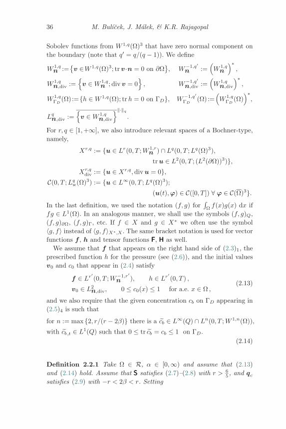
36 M. Bulıcek, J. Malek, & K.R. Rajagopal
Sobolev functions from W 1,q(Ω)3 that have zero normal component onthe boundary (note that q′ = q/(q − 1)). We define
W 1,qn :=
{v ∈W 1,q(Ω)3; tr v ·n = 0 on ∂Ω
}, W−1,q′
n :=(W 1,q
n
)∗,
W 1,qn,div :=
{v ∈W 1,q
n ; div v = 0}, W−1,q′
n,div :=(W 1,q
n,div
)∗,
W 1,qΓD
(Ω):={h ∈W 1,q(Ω); trh = 0 on ΓD}, W−1,q′ΓD
(Ω):=(W 1,q
ΓD(Ω)
)∗,
Lqn,div :=
{v ∈W 1,q
n,div
}‖·‖q
.
For r, q ∈ [1,+∞], we also introduce relevant spaces of a Bochner-type,namely,
Xr,q := {u ∈ Lr(0, T ;W 1,rn ) ∩ Lq(0, T ;Lq(Ω)3),
tr u ∈ L2(0, T ; (L2(∂Ω))3)},Xr,q
div := {u ∈ Xr,q,div u = 0},C(0, T ;Lq
w(Ω)3) := {u ∈ L∞(0, T ;Lq(Ω)3);
(u(t),ϕ) ∈ C([0, T ]) ∀ ϕ ∈ C(Ω)3}.In the last definition, we used the notation (f, g) for
∫Ωf(x)g(x) dx if
fg ∈ L1(Ω). In an analogous manner, we shall use the symbols (f, g)Q,(f, g)∂Ω, (f, g)Γ, etc. If f ∈ X and g ∈ X∗ we often use the symbol〈g, f〉 instead of 〈g, f〉X∗,X . The same bracket notation is used for vectorfunctions f , h and tensor functions FFF, HHH as well.
We assume that f that appears on the right hand side of (2.3)1, theprescribed function h for the pressure (see (2.6)), and the initial valuesv0 and c0 that appear in (2.4) satisfy
f ∈ Lr′(0, T ;W−1,r′
n ), h ∈ Lr′(0, T ) ,
v0 ∈ L2n,div, 0 ≤ c0(x) ≤ 1 for a.e. x ∈ Ω ,
(2.13)
and we also require that the given concentration cb on ΓD appearing in(2.5)4 is such that
for n := max {2, r/(r − 2β)} there is a cb ∈ L∞(Q) ∩ Ln(0, T ;W 1,n(Ω)),
with cb,t ∈ L1(Q) such that 0 ≤ tr cb = cb ≤ 1 on ΓD.
(2.14)
Definition 2.2.1 Take Ω ∈ R, α ∈ [0,∞) and assume that (2.13)and (2.14) hold. Assume that SSS satisfies (2.7)–(2.8) with r > 6
5 , and qc
satisfies (2.9) with −r < 2β < r. Setting
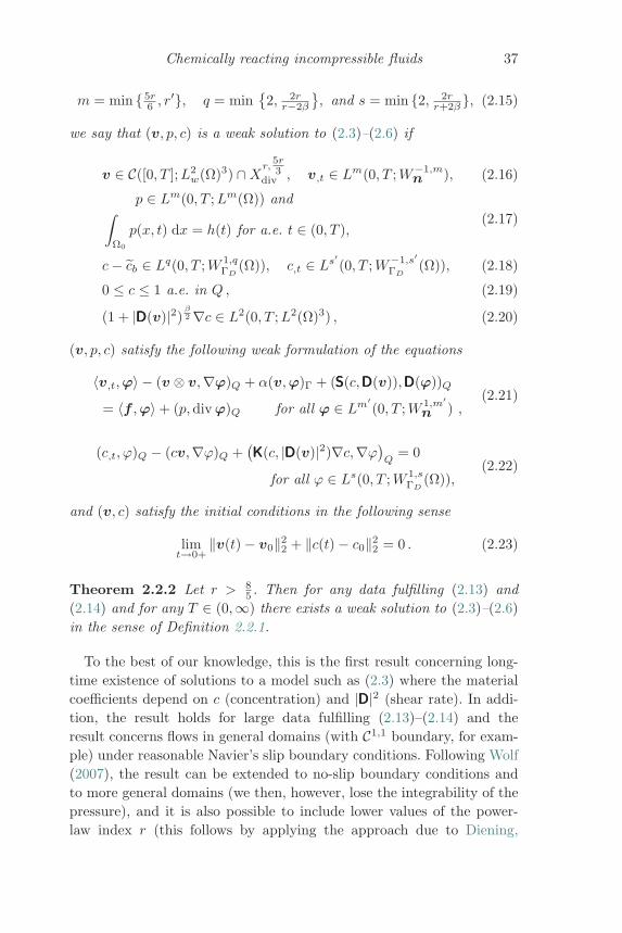
Chemically reacting incompressible fluids 37
m = min { 5r6 , r
′}, q = min{
2, 2rr−2β
}, and s = min {2, 2r
r+2β }, (2.15)
we say that (v, p, c) is a weak solution to (2.3)–(2.6) if
v ∈ C([0, T ];L2w(Ω)3) ∩Xr,
5r3
div , v,t ∈ Lm(0, T ;W−1,mn ), (2.16)
p ∈ Lm(0, T ;Lm(Ω)) and∫Ω0
p(x, t) dx = h(t) for a.e. t ∈ (0, T ),(2.17)
c− cb ∈ Lq(0, T ;W 1,qΓD
(Ω)), c,t ∈ Ls′(0, T ;W−1,s′
ΓD(Ω)), (2.18)
0 ≤ c ≤ 1 a.e. in Q , (2.19)
(1 + |DDD(v)|2)β2 ∇c ∈ L2(0, T ;L2(Ω)3) , (2.20)
(v, p, c) satisfy the following weak formulation of the equations
〈v,t,ϕ〉 − (v ⊗ v,∇ϕ)Q + α(v,ϕ)Γ + (SSS(c,DDD(v)),DDD(ϕ))Q
= 〈f ,ϕ〉 + (p,div ϕ)Q for all ϕ ∈ Lm′(0, T ;W 1,m′
n ) ,(2.21)
(c,t, ϕ)Q − (cv,∇ϕ)Q +(KKK(c, |DDD(v)|2)∇c,∇ϕ)
Q= 0
for all ϕ ∈ Ls(0, T ;W 1,sΓD
(Ω)),(2.22)
and (v, c) satisfy the initial conditions in the following sense
limt→0+
‖v(t) − v0‖22 + ‖c(t) − c0‖2
2 = 0 . (2.23)
Theorem 2.2.2 Let r > 85 . Then for any data fulfilling (2.13) and
(2.14) and for any T ∈ (0,∞) there exists a weak solution to (2.3)–(2.6)in the sense of Definition 2.2.1.
To the best of our knowledge, this is the first result concerning long-time existence of solutions to a model such as (2.3) where the materialcoefficients depend on c (concentration) and |DDD|2 (shear rate). In addi-tion, the result holds for large data fulfilling (2.13)–(2.14) and theresult concerns flows in general domains (with C1,1 boundary, for exam-ple) under reasonable Navier’s slip boundary conditions. Following Wolf(2007), the result can be extended to no-slip boundary conditions andto more general domains (we then, however, lose the integrability of thepressure), and it is also possible to include lower values of the power-law index r (this follows by applying the approach due to Diening,
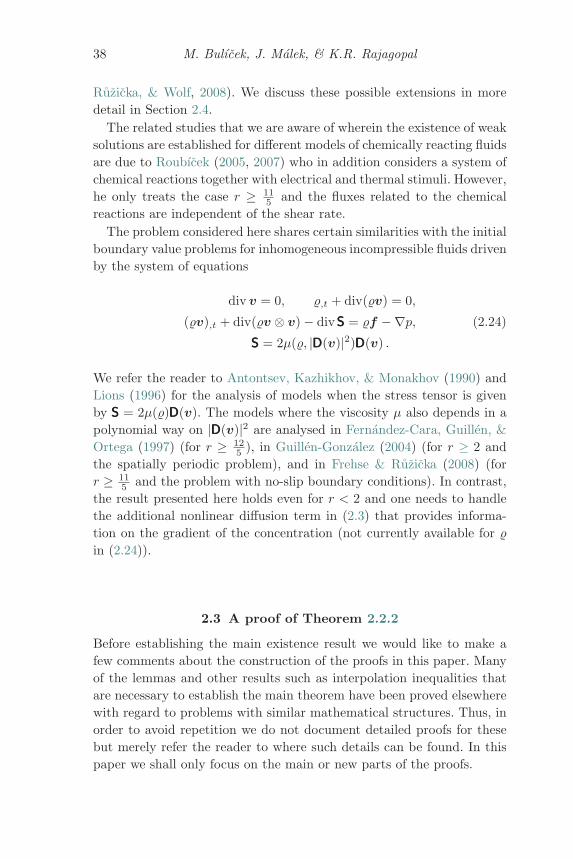
38 M. Bulıcek, J. Malek, & K.R. Rajagopal
Ruzicka, & Wolf, 2008). We discuss these possible extensions in moredetail in Section 2.4.
The related studies that we are aware of wherein the existence of weaksolutions are established for different models of chemically reacting fluidsare due to Roubıcek (2005, 2007) who in addition considers a system ofchemical reactions together with electrical and thermal stimuli. However,he only treats the case r ≥ 11
5 and the fluxes related to the chemicalreactions are independent of the shear rate.
The problem considered here shares certain similarities with the initialboundary value problems for inhomogeneous incompressible fluids drivenby the system of equations
div v = 0, �,t + div(�v) = 0,
(�v),t + div(�v ⊗ v) − divSSS = �f −∇p,SSS = 2μ(�, |DDD(v)|2)DDD(v) .
(2.24)
We refer the reader to Antontsev, Kazhikhov, & Monakhov (1990) andLions (1996) for the analysis of models when the stress tensor is givenby SSS = 2μ(�)DDD(v). The models where the viscosity μ also depends in apolynomial way on |DDD(v)|2 are analysed in Fernandez-Cara, Guillen, &Ortega (1997) (for r ≥ 12
5 ), in Guillen-Gonzalez (2004) (for r ≥ 2 andthe spatially periodic problem), and in Frehse & Ruzicka (2008) (forr ≥ 11
5 and the problem with no-slip boundary conditions). In contrast,the result presented here holds even for r < 2 and one needs to handlethe additional nonlinear diffusion term in (2.3) that provides informa-tion on the gradient of the concentration (not currently available for �in (2.24)).
2.3 A proof of Theorem 2.2.2
Before establishing the main existence result we would like to make afew comments about the construction of the proofs in this paper. Manyof the lemmas and other results such as interpolation inequalities thatare necessary to establish the main theorem have been proved elsewherewith regard to problems with similar mathematical structures. Thus, inorder to avoid repetition we do not document detailed proofs for thesebut merely refer the reader to where such details can be found. In thispaper we shall only focus on the main or new parts of the proofs.
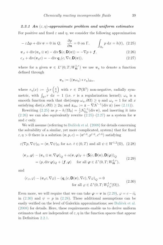
Chemically reacting incompressible fluids 39
2.3.1 An (ε, η)-approximate problem and uniform estimates
For positive and fixed ε and η, we consider the following approximation
− εΔp+ div v = 0 in Q,∂p
∂n= 0 on Γ,
∫Ω0
p dx = h(t), (2.25)
v,t + div(vη ⊗ v) − divSSS(c,DDD(v)) = −∇p+ f , (2.26)
c,t + div(vηc) = −div qc(c,∇c,DDD(v)), (2.27)
where for a given v ∈ Lr(0, T ;W 1,rn ) we use vη to denote a function
defined through
vη := ((vωη) ∗ rη)div,
where rη(x) := 1η3 r
(xη
)with r ∈ D(R3) non-negative, radially sym-
metric, with∫
R3 r dx = 1 (i.e. r is a regularization kernel); ωη is asmooth function such that dist(supp ωη, ∂Ω) ≥ η and ωη = 1 for all xsatisfying dist(x, ∂Ω) ≥ 2η; and zdiv := z −∇N−1(div z) (see (2.11)).
Rewriting (2.25) as p − h/|Ω0| = 1εN−1
Ω0(div v), and inserting it into
(2.26) we can also equivalently rewrite (2.25)–(2.27) as a system for v
and c only.We will assume (referring to Bulıcek et al. (2008) for details concerning
the solvability of a similar, yet more complicated, system) that for fixedε, η > 0 there is a solution (v, p, c) = (vε,η, pε,η, cε,η) satisfying
ε(∇p,∇ψ)Ω = (v,∇ψ)Ω for a.e. t ∈(0, T ) and all ψ ∈W 1,2(Ω), (2.28)
〈v,t,ϕ〉 − (vη ⊗ v,∇ϕ)Q + α(v,ϕ)Γ + (SSS(c,DDD(v),DDD(ϕ))Q
= (p,div ϕ)Q + 〈f ,ϕ〉 for all ϕ ∈ Lr(0, T ;W 1,rn ),
(2.29)
and
〈c,t, ϕ〉 − (vηc,∇ϕ) − (qc(c,DDD(v),∇c),∇ϕ)Q = 0
for all ϕ ∈ Ls(0, T ;W 1,sΓD
(Ω)).(2.30)
Even more, we will require that we can take ϕ = v in (2.29), ϕ = c− cbin (2.30) and ψ = p in (2.28). These additional assumptions can beeasily verified on the level of Galerkin approximations; see Bulıcek et al.(2008) for details. Here, these requirements enable us to derive uniformestimates that are independent of ε, η in the function spaces that appearin Definition 2.2.1.
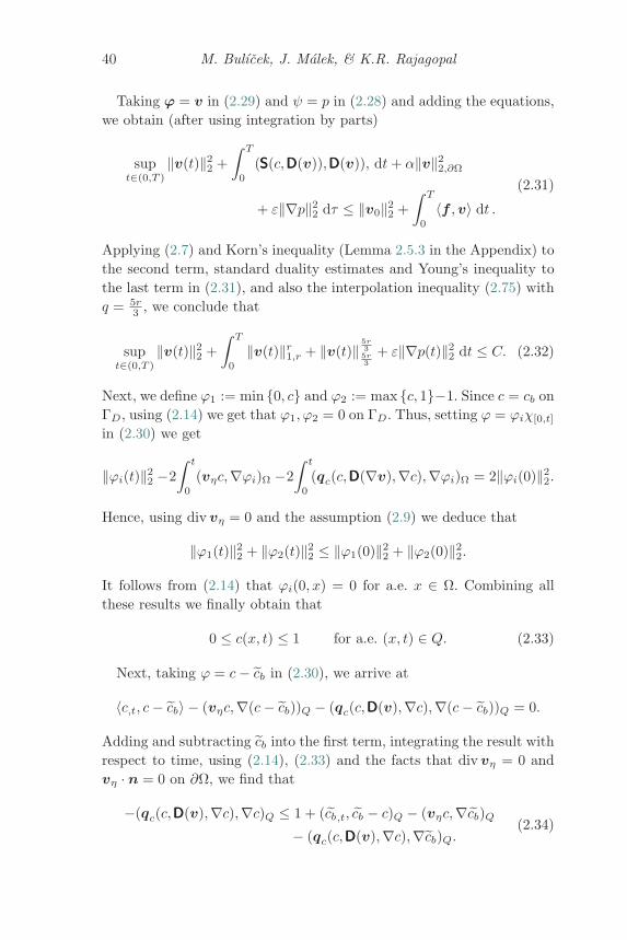
40 M. Bulıcek, J. Malek, & K.R. Rajagopal
Taking ϕ = v in (2.29) and ψ = p in (2.28) and adding the equations,we obtain (after using integration by parts)
supt∈(0,T )
‖v(t)‖22 +
∫ T
0
(SSS(c,DDD(v)),DDD(v)), dt+ α‖v‖22,∂Ω
+ ε‖∇p‖22 dτ ≤ ‖v0‖2
2 +∫ T
0
〈f ,v〉 dt .
(2.31)
Applying (2.7) and Korn’s inequality (Lemma 2.5.3 in the Appendix) tothe second term, standard duality estimates and Young’s inequality tothe last term in (2.31), and also the interpolation inequality (2.75) withq = 5r
3 , we conclude that
supt∈(0,T )
‖v(t)‖22 +
∫ T
0
‖v(t)‖r1,r + ‖v(t)‖ 5r
35r3
+ ε‖∇p(t)‖22 dt ≤ C. (2.32)
Next, we define ϕ1 := min {0, c} and ϕ2 := max {c, 1}−1. Since c = cb onΓD, using (2.14) we get that ϕ1, ϕ2 = 0 on ΓD. Thus, setting ϕ = ϕiχ[0,t]
in (2.30) we get
‖ϕi(t)‖22 −2
∫ t
0
(vηc,∇ϕi)Ω −2∫ t
0
(qc(c,DDD(∇v),∇c),∇ϕi)Ω = 2‖ϕi(0)‖22.
Hence, using div vη = 0 and the assumption (2.9) we deduce that
‖ϕ1(t)‖22 + ‖ϕ2(t)‖2
2 ≤ ‖ϕ1(0)‖22 + ‖ϕ2(0)‖2
2.
It follows from (2.14) that ϕi(0, x) = 0 for a.e. x ∈ Ω. Combining allthese results we finally obtain that
0 ≤ c(x, t) ≤ 1 for a.e. (x, t) ∈ Q. (2.33)
Next, taking ϕ = c− cb in (2.30), we arrive at
〈c,t, c− cb〉 − (vηc,∇(c− cb))Q − (qc(c,DDD(v),∇c),∇(c− cb))Q = 0.
Adding and subtracting cb into the first term, integrating the result withrespect to time, using (2.14), (2.33) and the facts that div vη = 0 andvη · n = 0 on ∂Ω, we find that
−(qc(c,DDD(v),∇c),∇c)Q ≤ 1 + (cb,t, cb − c)Q − (vηc,∇cb)Q
− (qc(c,DDD(v),∇c),∇cb)Q.(2.34)
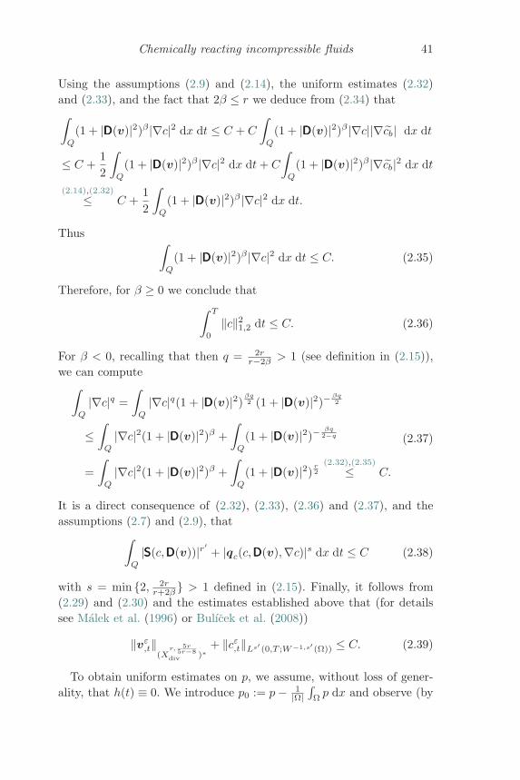
Chemically reacting incompressible fluids 41
Using the assumptions (2.9) and (2.14), the uniform estimates (2.32)and (2.33), and the fact that 2β ≤ r we deduce from (2.34) that∫
Q
(1 + |DDD(v)|2)β |∇c|2 dx dt ≤ C + C
∫Q
(1 + |DDD(v)|2)β |∇c||∇cb| dx dt
≤ C +12
∫Q
(1 + |DDD(v)|2)β |∇c|2 dx dt+ C
∫Q
(1 + |DDD(v)|2)β |∇cb|2 dx dt
(2.14),(2.32)
≤ C +12
∫Q
(1 + |DDD(v)|2)β |∇c|2 dx dt.
Thus ∫Q
(1 + |DDD(v)|2)β |∇c|2 dx dt ≤ C. (2.35)
Therefore, for β ≥ 0 we conclude that∫ T
0
‖c‖21,2 dt ≤ C. (2.36)
For β < 0, recalling that then q = 2rr−2β > 1 (see definition in (2.15)),
we can compute∫Q
|∇c|q =∫
Q
|∇c|q(1 + |DDD(v)|2)βq2 (1 + |DDD(v)|2)−
βq2
≤∫
Q
|∇c|2(1 + |DDD(v)|2)β +∫
Q
(1 + |DDD(v)|2)−βq2−q
=∫
Q
|∇c|2(1 + |DDD(v)|2)β +∫
Q
(1 + |DDD(v)|2)r2
(2.32),(2.35)
≤ C.
(2.37)
It is a direct consequence of (2.32), (2.33), (2.36) and (2.37), and theassumptions (2.7) and (2.9), that∫
Q
|SSS(c,DDD(v))|r′+ |qc(c,DDD(v),∇c)|s dx dt ≤ C (2.38)
with s = min {2, 2rr+2β } > 1 defined in (2.15). Finally, it follows from
(2.29) and (2.30) and the estimates established above that (for detailssee Malek et al. (1996) or Bulıcek et al. (2008))
‖vε,t‖
(Xr, 5r
5r−8div )∗
+ ‖cε,t‖Ls′ (0,T ;W−1,s′ (Ω)) ≤ C. (2.39)
To obtain uniform estimates on p, we assume, without loss of gener-ality, that h(t) ≡ 0. We introduce p0 := p− 1
|Ω|∫Ωp dx and observe (by
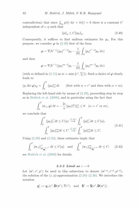
42 M. Bulıcek, J. Malek, & K.R. Rajagopal
contradiction) that since∫Ω0p(t) dx = h(t) = 0 there is a constant C
independent of ε, η such that
‖p‖q ≤ C‖p0‖q. (2.40)
Consequently, it suffices to find uniform estimates for p0. For thispurpose, we consider ϕ in (2.29) first of the form
ϕ = ∇N−1(|p0|r′−2p0 − 1|Ω|
∫Ω
|p0|r′−2p0 dx)
and then
ϕ = ∇N−1(|p0|m−2p0 − 1|Ω|
∫Ω
|p0|m−2p0 dx)
(with m defined in (2.15) as m = min {r′, 5r6 }). Such a choice of ϕ clearly
leads to
(p,div ϕ)Q =∫ T
0
‖p0‖αα dt (first with α = r′ and then with α = m).
Replacing the left-hand side by means of (2.29), proceeding step by stepas in Bulıcek et al. (2008), and in particular using the fact that∫ T
0
〈v,t,ϕ〉dt = −2εα‖p0(T )‖α
α ≤ 0 (α = r′ or m) ,
we conclude that∫ T
0
‖p0‖r′r′dt ≤ C(η)
(2.40)=⇒
∫ T
0
‖p‖r′r′dt ≤ C(η),∫ T
0
‖p0‖mmdt ≤ C
(2.40)=⇒
∫ T
0
‖p‖mmdt ≤ C.
(2.41)
Using (2.29) and (2.32), these estimates imply that∫ T
0
‖v,t‖r′
W−1,r′n
dt ≤ C(η) and∫ T
0
‖v,t‖mW−1,m
ndt ≤ C; (2.42)
see Bulıcek et al. (2008) for details.
2.3.2 Limit as ε→ 0
Let (vε, cε, pε) be used in this subsection to denote (vε,η, cε,η, pε,η),the solution of the (ε, η)-approximation (2.28)–(2.30). We introduce thenotation
qεc := qc(cε,DDD(vε),∇cε) and SSSε := SSS(cε,DDD(vε)) .
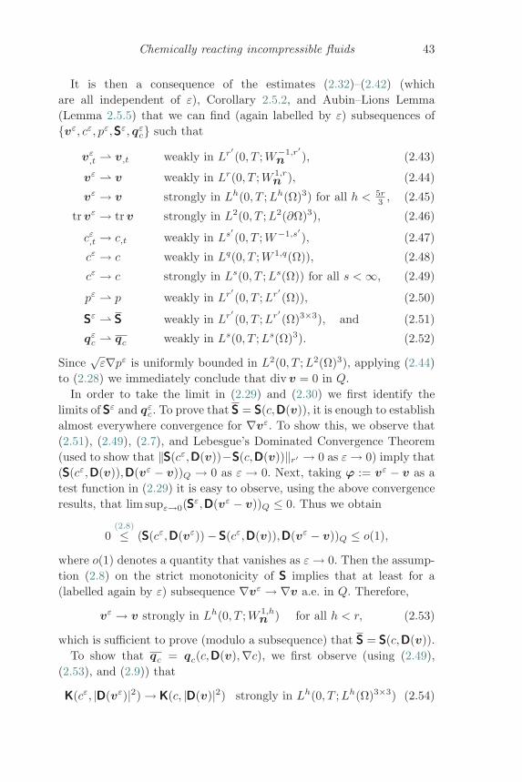
Chemically reacting incompressible fluids 43
It is then a consequence of the estimates (2.32)–(2.42) (whichare all independent of ε), Corollary 2.5.2, and Aubin–Lions Lemma(Lemma 2.5.5) that we can find (again labelled by ε) subsequences of{vε, cε, pε,SSSε, qε
c} such that
vε,t ⇀ v,t weakly in Lr′
(0, T ;W−1,r′n ), (2.43)
vε ⇀ v weakly in Lr(0, T ;W 1,rn ), (2.44)
vε → v strongly in Lh(0, T ;Lh(Ω)3) for all h < 5r3 , (2.45)
tr vε → tr v strongly in L2(0, T ;L2(∂Ω)3), (2.46)
cε,t → c,t weakly in Ls′(0, T ;W−1,s′
), (2.47)
cε → c weakly in Lq(0, T ;W 1,q(Ω)), (2.48)
cε → c strongly in Ls(0, T ;Ls(Ω)) for all s <∞, (2.49)
pε ⇀ p weakly in Lr′(0, T ;Lr′
(Ω)), (2.50)
SSSε ⇀ SSS weakly in Lr′(0, T ;Lr′
(Ω)3×3), and (2.51)
qεc ⇀ qc weakly in Ls(0, T ;Ls(Ω)3). (2.52)
Since√ε∇pε is uniformly bounded in L2(0, T ;L2(Ω)3), applying (2.44)
to (2.28) we immediately conclude that div v = 0 in Q.In order to take the limit in (2.29) and (2.30) we first identify the
limits of SSSε and qεc. To prove that SSS = SSS(c,DDD(v)), it is enough to establish
almost everywhere convergence for ∇vε. To show this, we observe that(2.51), (2.49), (2.7), and Lebesgue’s Dominated Convergence Theorem(used to show that ‖SSS(cε,DDD(v))−SSS(c,DDD(v))‖r′ → 0 as ε→ 0) imply that(SSS(cε,DDD(v)),DDD(vε − v))Q → 0 as ε → 0. Next, taking ϕ := vε − v as atest function in (2.29) it is easy to observe, using the above convergenceresults, that lim supε→0(SSSε,DDD(vε − v))Q ≤ 0. Thus we obtain
0(2.8)
≤ (SSS(cε,DDD(vε)) − SSS(cε,DDD(v)),DDD(vε − v))Q ≤ o(1),
where o(1) denotes a quantity that vanishes as ε→ 0. Then the assump-tion (2.8) on the strict monotonicity of SSS implies that at least for a(labelled again by ε) subsequence ∇vε → ∇v a.e. in Q. Therefore,
vε → v strongly in Lh(0, T ;W 1,hn ) for all h < r, (2.53)
which is sufficient to prove (modulo a subsequence) that SSS = SSS(c,DDD(v)).To show that qc = qc(c,DDD(v),∇c), we first observe (using (2.49),
(2.53), and (2.9)) that
KKK(cε, |DDD(vε)|2) → KKK(c, |DDD(v)|2) strongly in Lh(0, T ;Lh(Ω)3×3) (2.54)
44 M. Bulıcek, J. Malek, & K.R. Rajagopal
for all h ∈ [1, r2β ) if β > 0 and all h ∈ (1,∞) if β ≤ 0. Thus, for β ≤ 0 it
is a direct consequence of the convergence properties shown above thatqc = qc(c,DDD(v),∇c). For β ≥ 0 we proceed more carefully. Using thenotation κε := |KKK(cε,DDD(vε))|, (2.54) implies that for all h ∈ (1,∞)
KKK(cε, |DDD(vε)|2)κε
→ KKK(c, |DDD(v)|2)κ
strongly in Lh(0, T ;Lh(Ω)3×3) .
Thus, to identify qc, it is enough to identify κ∇c (here the symbol κ∇cdenotes the weak limit of κε∇cε). Then (2.9), (2.33), and (2.35) imply(modulo a subsequence) that
√κε∇cε ⇀ √
κ∇c weakly in L2(Q). Thus,having 2β < r and the strong convergence (2.54), we know that
√κε →√
κ strongly in L2(Q). Hence, to identify the limit qc it is enough toidentify the limit
√κ∇c. Using this procedure inductively, we see that
it is enough that for some k ∈ N we have(κε)2−k
∇cε ⇀ κ2−k∇c weakly in L1(Q). (2.55)
Hence, we find k such that(
r2k−1
β
)′> q′. Then it is a consequence of
(2.54) and (2.48) that the convergence (2.55) is valid and this finishesthe proof of the convergence of qε
c.Finally, having all these convergence results (2.43)–(2.52) in hand
together with the identification of the limit of the nonlinear terms, wecan take the limit ε → 0 in (2.29) and in (2.30) in a standard way andconclude that for any η > 0 the triplet (v, c, p) := (vη, cη, pη) satisfies
〈v,t,ϕ〉 − (vη ⊗ v,∇ϕ)Q + (SSS(c,DDD(v)),∇ϕ)Q
+ α(v,ϕ)Γ − (p,div ϕ)Q = 〈f ,ϕ〉for all ϕ ∈ Lr(0, T ;W 1,r
n ) such that tr ϕ ∈ L2(Γ),
(2.56)
and
〈c,t, ϕ〉 − (vηc,∇ϕ)Q = (qc(c,DDD(v),∇c),∇ϕ)Q
for all ϕ ∈ Lm′(0, T ;W 1,m′
(Ω)) such that ϕ|ΓD = 0.(2.57)
The attainment of initial conditions is again standard and can beproved by using the same methods as those described in Malek et al.(1996).
2.3.3 Limit as η → 0
Let (vη, cη, pη,SSSη, qηc ), the solution of the η-approximation, satisfy (2.56)
and (2.57). Our final goal is to take the limit η → 0 in (2.56) and in
Chemically reacting incompressible fluids 45
(2.57), and to establish the existence of a suitable weak solution to ouroriginal problem.
Using weak lower semicontinuity of appropriate norms, we find that(2.32)–(2.39), (2.41)2 and (2.42)2 hold. These estimates together withthe Aubin–Lions Lemma (Lemma 2.5.5) and Corollary 2.5.2 are suf-ficient to find a (labelled again by ε) subsequence of (vη, cη, pη) suchthat
vη,t ⇀ v,t weakly in Lm(0, T ;W−1,m
n ) ∩ (Xr, 5r5r−8 )∗, (2.58)
vη ⇀ v weakly in Lr(0, T ;W 1,rn ), (2.59)
vη → v strongly in Lh(0, T ;Lh(Ω)3) for all h < 5r3 , (2.60)
tr vη → tr v strongly in L2(0, T ;L2(∂Ω)3), (2.61)
cη,t ⇀ c,t weakly in Ls′(0, T ;W−1,s′
(Ω)), (2.62)
cη ⇀ c weakly in Lq(0, T ;W 1,q(Ω)), (2.63)
cη → c strongly in Lh(0, T ;Lh(Ω)) for all h <∞, (2.64)
pη ⇀ p weakly in Lm(0, T ;Lm(Ω)), (2.65)
SSSη → SSS weakly in Lr′(0, T ;Lr′
(Ω)3×3), and (2.66)
qηc → qc weakly in Ls(0, T ;Ls(Ω)3). (2.67)
Assume for a moment that DDD(vη) converges to DDD(v) almost everywherein Q. Then using the same procedure as in Subsection 2.3.2 we getqc = qc(c,DDD(v)∇c). Then we are able to take the limit in (2.57) and toachieve (2.22).
Thus it remains to show that ∇vη converges a.e. in Q. To do this,we follow the approach described in Boccardo & Murat (1992), Frehse,Malek, & Steinhauer (2000), or Bulıcek et al. (2008). We define
gη := |∇vη|r + |∇v|r + (|SSSη| + |SSS|) (|DDD(vη)| + |DDD(v)|) .
It follows from (2.59) and (2.66) that there is K ∈ [1,∞) so thatfor all η
0 ≤∫ T
0
∫Ω
gη dx dt ≤ K .
46 M. Bulıcek, J. Malek, & K.R. Rajagopal
Let ε∗ > 0 be arbitrary. Then the following statement is proved inBulıcek et al. (2008):
There exist L ≤ ε∗
K, a subsequence {vj}∞j=1 ⊂ {vη}η>0,
and sets Ej :={
(t, x) ∈ Q;L2 ≤ |vj(t, x) − v(t, x)| < L}
such that∫
Ej
gj dx dt ≤ ε∗.
(2.68)
For the obtained sequence {vj}∞j=1 and L we define uj and the sets Qj as
uj :=(vj − v)(
1 − min{
|v−vj |L , 1
});
Qj :={
(t, x) ∈ Q; |v − vj | < L}.
By using (2.59), (2.60), and the fact that |uj | ≤ L in Q we have (asj → ∞)
uj ⇀ 0 weakly in Lr(0, T ;W 1,rn ), (2.69)
uj → 0 strongly in Ls(0, T ;Ls(Ω)3) ∀s <∞, (2.70)
tr uj → 0 strongly in L2(0, T ;L2(∂Ω)3). (2.71)
Since (see equation (2.60) in Bulıcek et al., 2008, for details)∫ T
0
‖div uj‖rr dt ≤ Cε∗,
the Helmholtz decomposition uj = ujdiv + ∇guj
then implies that∫ T
0
‖guj‖r2,r dt ≤ Cε∗ (2.72)
and
ujdiv → 0 strongly in Ls(0, T ;Ls(Ω)3) for all s <∞.
Using the assumption (2.9) we have
0 ≤ (SSS(cj ,DDD(vj)) − SSS(cj ,DDD(v)),DDD(vj − v))Qj
= −(SSS(cj ,DDD(v)),DDD(vj − v))Qj + (SSS(cj ,DDD(vj)),DDD(vj − v))Qj
=: Y1 + Y2.
By virtue of (2.64), the Lebesgue Dominated Convergence Theorem and(2.7), we observe that
SSS(cj ,DDD(v)) → SSS(c,DDD(v)) strongly in Lr′(0, T ;Lr′
(Ω)3×3).
Chemically reacting incompressible fluids 47
Therefore (as j → ∞)
Y1 := (SSS(cj ,DDD(v)),DDD(v − vj))Qj
= (SSS(cj ,DDD(v)),DDD(uj))Q + (SSS(cj ,DDD(v)),DDD((v − vj) |v−vj |L ))Qj
(2.3.3)
≤(2.69)
o(1) + (SSS(cj ,DDD(v)),DDD((v − vj) |v−vj |L ))Qj\Ej
+ (SSS(cj ,DDD(v)),DDD((v − vj) |v−vj |L ))Ej
(2.68)
≤ o(1) + CL+ Cε∗ ≤ o(1) + Cε∗ ,
where o(1) → 0 as j → ∞. To estimate Y2 we set ϕ = ujdiv in (2.56) and
denoting SSSj := SSS(cj ,DDD(vj)) obtain
Y2 := (SSSj ,DDD(vj − v))Qj = (SSSj ,DDD(uj))Q + (SSSj ,DDD((v − vj) |v−vj |L ))Qj
= (SSSj ,DDD(ujdiv))Q + (SSSj ,DDD(∇guj
))Q + (SSSj ,DDD((v − vj) |v−vj |L ))Qj
(2.68)
≤(2.72)
(SSSj ,DDD(ujdiv))Q + Cε∗
(2.56)= :
4∑i=1
Ii + Cε∗,
where2
I1 = −〈vj,t,u
jdiv〉 = −〈v,t,u
jdiv〉 + 〈v,t − vj
,t,ujdiv〉
≤ o(1) + 〈v,t − vj,t,u
jdiv〉
div v−vj=0= o(1) + 〈v,t − vj,t,u
j〉 ≤ o(1),
I2 = −(
[∇vj ]vjη(j),u
jdiv
)Q≤ C‖uj‖ 5r
5r−8 ,Q‖vj‖ 5r3 ,Q‖∇vj‖r,Q
(2.70)= o(1),
I3 = −α(vj ,ujdiv)Γ ≤ C‖uj‖L2(Γ)
(2.71)= o(1), and
I4 = 〈f ,ujdiv〉 = o(1).
Thus, we can conclude that for θ < 1∫Q
|(SSSj − SSS(cj ,DDD(v))) ·DDD(vj − v)|θ =∫
Qj
| . . . |θ +∫
Q\Qj
| . . . |θ
≤ C(Y1 + Y2)θ + C|Q \Qj |1−θ ≤ o(1)
and using strict monotonicity of SSS, i.e. the assumption (2.9) we obtainthat DDD(vj) converges to DDD(v) a.e. in Q. Thus with the help of Vitali’sTheorem, it is standard to take limit in (2.56) to obtain (2.21). Theproof is complete.
2For details concerning the estimate of I1 see Bulıcek et al. (2008).
48 M. Bulıcek, J. Malek, & K.R. Rajagopal
2.4 Extensions of Theorem 2.2.2
This section is devoted to the formulation of extensions that are notproved in detail anywhere but are direct consequences of the approachesdescribed here and those presented in recent studies by Wolf (2007)and Diening et al. (2008). These extensions are focused on includinggeneral domains with no smoothness of the boundary, incorporating no-slip boundary conditions, and lowering the power-law index r. We wishto underline that to the best of our knowledge we can deal with globallyintegrable pressure for the low exponents of r only for domains of classR and for Navier’s slip boundary conditions, the case that is studied inprevious sections.
We first formulate the result for the same range of r as in Theorem2.2.2 and for no-slip boundary conditions (corresponding to α = ∞in (2.5)1) which also enables us to consider any bounded domain. Thepressure is omitted from the weak formulation. As the pressure is notin general an integrable function it is also no longer clear how to fix itsmean value over any spatial subdomain.
Theorem 2.4.1 Let Ω be a bounded domain and let (2.13)–(2.14) hold(with the exception of the condition fixing the pressure). Assume that SSS
satisfies (2.7)–(2.8) with r > 85 , and qc satisfies (2.9) with −r < 2β < r.
Let m, q and s be defined as in (2.15). Then there is a weak solution(v, c) of (2.3)–(2.6) such that
v ∈ C([0, T ];L2w(Ω)3) ∩ Lr(0, T ;W 1,r
0,div), v,t ∈ Lm(0, T ;W−1,m0,div ),
c− cb ∈ Lq(0, T ;W 1,qΓD
(Ω)), c,t ∈ Ls′(0, T ;W−1,s′
ΓD(Ω)),
0 ≤ c ≤ 1 a.e. in Q ,
(1 + |DDD(v)|2)β2 ∇c ∈ L2(0, T ;L2(Ω)3) ,
(v, c) satisfy the following weak formulation
〈v,t,ϕ〉 − (v ⊗ v,∇ϕ)Q + α(v,ϕ)Γ + (SSS(c,DDD(v)),DDD(ϕ))Q = 〈f ,ϕ〉for all ϕ ∈ Lm′
(0, T ;W 1,m′0,div) ,
(c,t, ϕ)Q − (cv,∇ϕ)Q +(KKK(c, |DDD(v)|2)∇c,∇ϕ)
Q= 0
for all ϕ ∈ Ls(0, T ;W 1,sΓD
(Ω)),
and (v, c) attain the initial conditions as in (2.23).
The next theorem extends the result stated in Theorem 2.2.2 also tothe case r ∈ (6/5, 8/5].
Chemically reacting incompressible fluids 49
Theorem 2.4.2 Let 65 < r ≤ 8
5 . Then for any data fulfilling (2.13)–(2.14) and for any T ∈ (0,∞) there exists a weak solution to (2.3)–(2.6)in the sense of Definition 2.2.1.
The extension of the existence result in the sense of Theorem 2.4.1 tono-slip boundary conditions for r ∈ (6/5, 8/5] can be also proved. Weskip the formulation.
Our final remark concerns the possible extension of the result estab-lished here and formulated in the above theorem to models describingunsteady flows of incompressible chemically reacting and heat conduct-ing fluids. Such a problem requires one to consider the full thermo-dynamical system including the balance of energy and possibly alsothe second law of thermodynamics in combination with the convection-diffusion equation for c. An interested reader could combine the resultsestablished here with those proved in Bulıcek et al. (2009) and Bulıceket al. (2008) where incompressible Navier–Stokes–Fourier-like systemsare analysed.
2.5 Appendix
The following lemmas summarize helpful properties of functions belong-ing to certain Sobolev spaces.
Lemma 2.5.1 Let 1 < q1, q2 <∞. Set
S := {v; v ∈ L∞(0, T ;L2(Ω)3)∩Lr(0, T ;W 1,rn ),v,t ∈ Lq1(0, T ;W−1,q2
n,div )}.If r > 3
2 and {vi}∞i=1 is bounded in S, then {tr vi}∞i=1 is precompact inLp(0, T ;Ls(∂Ω)3) for all p, s ∈ (1,∞) satisfying
p < s5r−63s−4 , max (2, r) ≤ s ≤ 2r
3−r . (2.73)
Proof See Bulıcek et al. (2008, Lemma 1.4) where an even more generalresult is proved.
Corollary 2.5.2 Let r > 85 . Let {vi}∞i=1 be bounded in S. Then
{tr vi}∞i=1 is precompact in L2(0, T ;L2(∂Ω)3).
Lemma 2.5.3 (Korn’s inequality) Let q ∈ (1,∞). Then there existsa positive constant C depending only on Ω and q such that for all v ∈W 1,q(Ω)3 that has trace tr v ∈ L2(∂Ω)3 the following inequality holds
C‖v‖1,q ≤ ‖DDD(v)‖q + ‖v‖L2(∂Ω). (2.74)
50 M. Bulıcek, J. Malek, & K.R. Rajagopal
Proof For the proof we refer the reader to a modification of the resultin Necas (1966) and Bulıcek et al. (2008).
Lemma 2.5.4 (Interpolation inequalities) For 2 ≤ q ≤ 3r3−r (if
6/5 < r < 3) and for any q ∈ [1,∞) if r ≥ 3 the following inequalityholds
‖z‖q ≤ ‖z‖6r−6q+2qr
q(5r−6)2 ‖z‖
3r(q−2)q(5r−6)1,r . (2.75)
Proof See Nirenberg (1966).
Lemma 2.5.5 (Aubin–Lions) Let V1, V2, V3 be reflexive separableBanach spaces such that
V1 ↪→↪→ V2 and V2 ↪→ V3.
Let 1 < p <∞, 1 ≤ q ≤ +∞ and 0 < T <∞. Then
{v; v ∈ Lp(0, T ;V1), v,t ∈ Lq(0, T ;V3)}is compactly embedded into Lp(0, T ;V2).
Proof See for example Simon (1987) or Feireisl (2004, Lemma 6.3).
Acknowledgements
The contribution of M. Bulıcek to this work was supported by theJindrich Necas Center for Mathematical Modeling, the project LC06052financed by MSMT. J. Malek’s contribution is a part of the researchproject MSM 0021620839 financed by MSMT; the support of GACR201/08/0315 and GACR 201/06/0352 is also acknowledged. K.R.Rajagopal thanks the National Science Foundation for its support.
ReferencesAdkins, J.E. (1963a) Non-linear diffusion. I. Diffusion and flow of mixtures of
fluids. Philos. Trans. Roy. Soc. London Ser. A 255, 607–633.Adkins, J.E. (1963b) Non-linear diffusion. II. Constitutive equations for mix-
tures of isotropic fluids. Philos. Trans. Roy. Soc. London Ser. A 255,635–648.
Anand, M. & Rajagopal, K.R. (2004) A shear-thinning viscoelastic fluid modelfor describing the flow of blood. International Journal of CardiovascularMedicine and Science 4, 59–68.
Chemically reacting incompressible fluids 51
Anand, M., Rajagopal, K., & Rajagopal, K.R. (2003) A model incorporatingsome of the mechanical and biochemical factors underlying clot formationand dissolution in flowing blood. J. Theor. Med. 5, no. 3-4, 183–218.
Anand, M., Rajagopal, K., & Rajagopal, K.R. (2005) A model for the for-mation and lysis of blood clots. Pathophysiology of Haemostasis andThrombosis 34, 109–120.
Antontsev, S.N., Kazhikhov, A.V., & Monakhov, V.N. (1990) Boundary valueproblems in mechanics of nonhomogeneous fluids. Studies in Mathematicsand its Applications 22, North-Holland Publishing Co., Amsterdam.
Atkin, R.J. & Craine, R.E. (1976a) Continuum theories of mixtures: applica-tions. J. Inst. Math. Appl. 17, no. 2, 153–207.
Atkin, R.J. & Craine, R.E. (1976b) Continuum theories of mixtures: basictheory and historical development. Quart. J. Mech. Appl. Math. 29, no.2, 209–244.
Boccardo, L. & Murat, F. (1992) Almost everywhere convergence of the gradi-ents of solutions to elliptic and parabolic equations. Nonlinear Anal. 19,no. 6, 581–597.
Bowen, R.M. (1975) Continuum physics III, Academic Press, New York.Bridges, C. & Rajagopal, K.R. (2006) Pulsatile flow of a chemically-reacting
nonlinear fluid. Comput. Math. Appl. 52, no. 6-7, 1131–1144.Brinkman, H.C. (1947a) A calculation of the viscous force exerted by a flowing
fluid on a dense swarm of particles. Applied Scientific Research A1,27–34.
Brinkman, H.C. (1947b) On the permeability of media consisting of closelypacked porous particles. Applied Scientific Research A1, 81–86.
Bulıcek, M., Malek, J., & Rajagopal, K.R. (2008) Mathematical analysis ofunsteady flows of fluids with pressure, shear-rate and temperature depen-dant material moduli, that slip at solid boundaries. SIAM J. Math. Anal,to appear.
Bulıcek, M., Feireisl, E., & Malek, J. (2009) Navier-Stokes-Fourier system forincompressible fluids with temperature dependent material coefficients.to appear in Nonlinear Analysis: Real World Applications, 10, 992–1015.
Darcy, H. (1856) Les Fontaines Publiques de La Ville de Dijon. VictorDalmont, Paris.
Diening, L., Ruzicka, M., & Wolf, J. (2008) Existence of weak solutions to theequations of non-stationary motion of non-Newtonian fluids with shearrate dependent viscosity. Ann. Scuola Norm. Sup. Pisa CI. Sci, to appear.
Fernandez-Cara, E., Guillen, F., & Ortega, R.R. (1997) Some theoreticalresults for viscoplastic and dilatant fluids with variable density. NonlinearAnal. 28, no. 6, 1079–1100.
Feireisl, E. (2004) Dynamics of viscous compressible fluids. Oxford Lec-ture Series in Mathematics and its Applications 26, Oxford UniversityPress, Oxford.
Forchheimer, P. (1901) Wasserbewegung Durch Boden. Zeits. V. Deutsch. Ing.45, 1781–1788.
Frehse, J., Malek, J., & Steinhauer, M. (2000) On existence results for fluidswith shear dependent viscosity - unsteady flows. Partial differential equa-tions (Praha, 1998). Res. Notes Math. 406, Chapman & Hall/CRC, BocaRaton, FL.
Frehse, J. & Ruzicka, M. (2008) Non-homogeneous generalized Newtonianfluids. Math. Z. 260, no. 2, 355–375.
52 M. Bulıcek, J. Malek, & K.R. Rajagopal
Green, A.E. & Naghdi, P.M. (1969) On Basic Equations for Mixtures. Quart.J. Mech. Appl. Math. 22, 427–438.
Gray, W.G. (1983) General conservation equations for multiphase systems 4.Constitutive theory including phase change. Adv. Water Resources 6,130–140.
Grisvard, P. (1985) Elliptic problems in nonsmooth domains. Monographsand Studies in Mathematics 24, Pitman (Advanced Publishing Pro-gram), Boston, MA.
Guillen-Gonzalez, F. (2004) Density-dependent incompressible fluids withnon-Newtonian viscosity. Czechoslovak Math. J. 54(129), no. 3, 637–656.
Hassanizadeh, M. (1986) Derivation of basic equations of mass transport inporous media, Part 1. Macroscopic balance laws. Adv. Water Resources9, 196–206.
Lions, P.L. (1996) Mathematical topics in fluid mechanics. Vol. 1. OxfordLecture Series in Mathematics and its Applications 3, The ClarendonPress Oxford University Press, New York.
Malek, J., Necas, J., Rokyta, M., & Ruzicka, M. (1996) Weak and measure-valued solutions to evolutionary PDEs. Chapman & Hall, London.
Necas, J. (1966) Seminaire Equations aux Derivees Partielles. Les Presses del’Universite.
Nirenberg, L. (1966) An extended interpolation inequality. Ann. Scuola Norm.Sup. Pisa (3) 20, 733–737.
Novotny, A. & Straskraba, I. (2004) Introduction to the mathematical the-ory of compressible flow. Oxford Lecture Series in Mathematics and itsApplications 27, Oxford University Press, Oxford.
Rajagopal, K.R. (2007) On a hierarchy of approximate models for flows ofincompressible fluids through porous solids. Math. Models Methods Appl.Sci. 17, no. 2, 215–252.
Rajagopal, K.R. & Tao, L. (1995) Mechanics of mixtures. World ScientificPublishing Co. Inc., River Edge, NJ.
Rayleigh, Lord (1883) Investigation of the character of the equilibrium of anincompressible heavy fluids of variable density. Proceedings of the LondonMathematical Society 14, 170–177.
Roubıcek, T. (2005) Incompressible ionized fluid mixtures: a non-Newtonianapproach. IASME Trans. 2, no. 7, 1190–1197.
Roubıcek, T. (2007) Incompressible ionized non-Newtonean fluid mixtures.SIAM J. Math. Anal. 39, no. 3, 863–890.
Simon, J. (1987) Compact sets in the space Lp(0, T ; B). Ann. Mat. Pura Appl.146, 65–96.
Thurston, G.B. (1972) Viscoelasticity of human blood. Biophysical Journal12, no. 9, 1205–1217.
Thurston, G.B. (1973) Frequency and shear rate dependence of viscoelasticityof blood. Biorheology 10, 375–381.
Truesdell, C.A. (1991) A first course in rational continuum mechanics 1,Academic Press, New York.
Wolf, J. (2007) Existence of weak solutions to the equations of non-stationarymotion of non-Newtonian fluids with shear rate dependent viscosity. J.Math. Fluid Mech. 9, no. 1, 104–138.
Yeleswarapu, K.K. (1996) Evaluation of Continuum Models for Characterizingthe Constitutive Behavior of Blood. PhD Thesis, University of Pittsburgh.
Chemically reacting incompressible fluids 53
Yeleswarapu, K.K., Kameneva, M. V., Rajagopal, K.R., & Antaki, J.F. (1998)The flow of blood in tubes: theory and experiment. Mechanics ResearchCommunication 25, 257–262.
Yih, C.S. (1965) Dynamics of non-homogeneous fluids. MacMillan, New York.Yih, C.S. (1980) Stratified flows. Academic Press, New York.
3
The uniqueness of Lagrangian trajectories inNavier–Stokes flows
Masoumeh Dashti & James C. RobinsonMathematics Institute, University of Warwick,
Coventry, CV4 7AL. [email protected]
Abstract
Given an initial condition in H(d/2)−1, the d-dimensional Navier–Stokesequations (d = 2, 3) have a unique solution; when d = 2 this solutionexists for all t ≥ 0, while when d = 3 its existence can only be guaran-teed on some time interval [0, T ). Given such a solution, we show byelementary methods (in the periodic case) that the Lagrangian par-ticle trajectories are also unique. In fact, we prove a general resultthat solutions of the ordinary differential equation X = u(X, t)are unique if u ∈ L2(0, T ;H(d/2)−1) and
√t u ∈ L2(0, T ;H(d/2)+1),
and verify that these conditions hold for the Navier–Stokes equationsvia some straightforward energy estimates. We also show that theLagrangian trajectories depend continuously on the Eulerian initial datau0 ∈ H(d/2)−1.
3.1 Introduction
We consider the Navier–Stokes equations
ut − νΔu+ (u · ∇)u+ ∇p = 0 ∇ · u = 0. (3.1)
In the two-dimensional case it is well known that an initial con-dition u0 ∈ L2 gives rise to a unique weak solution u withu ∈ L∞(0, T ;L2) ∩ L2(0, T ;H1) for every T > 0 (see Constantin &Foias, 1988, for example). In the three-dimensional case, if u0 ∈ H1/2
then (Kato & Fujita, 1962; Chemin et al., 2006) there is a unique solu-tion u ∈ L∞(0, T ;H1/2) ∩ L2(0, T ;H3/2) that exists for at least somesmall time interval [0, T ∗). In other words, for u0 ∈ H(d/2)−1 there existsa unique solution u ∈ L∞(0, T ;H(d/2)−1) ∩ L2(0, T ;Hd/2), d = 2, 3.
Using Littlewood–Paley theory, Chemin & Lerner (1995) showed thatfor flows on the whole of Rd (d = 2, 3) the associated Lagrangian
Published in Partial Differential Equations and Fluid Mechanics, edited byJames C. Robinson and Jose L. Rodrigo. c© Cambridge University Press 2009.
Lagrangian trajectories in the Navier–Stokes equations 55
trajectories – the paths traced out by ‘fluid particles’ – inherit thisuniqueness, despite the rough nature of the vector field u. Here we give amuch more elementary proof of the same result, in a form that is largelyindependent of the structure of the Navier–Stokes equations themselves.
For the sake of simplicity we restrict here to periodic boundary condi-tions and initial conditions that have zero average (a condition which ispreserved under the evolution). However, a similar analysis is also possi-ble in the more technically challenging case of flows in bounded domainswith no slip boundary conditions: for details see Dashti & Robinson(2009).
More precisely, the question is whether the solutions of the ordinarydifferential equation
X = u(X, t) X(0) = X0 (3.2)
are unique, when u(t) is a solution of the Navier–Stokes equations withu0 ∈ H(d/2)−1. An elementary computation – which uses the result
|u(X) − u(Y )| ≤ c‖u‖H(d/2)+1 |X − Y |(− log |X − Y |)1/2
due to Zuazua (2002) – shows that u does not have enough regularityto proceed in an entirely straightforward manner.
To this end, let X(t) and Y (t) be two solutions of (3.2) with X(0) =Y (0) = X0. Then with W (t) = X(t) − Y (t) one has
ddt
|W | ≤ |u(X, t) − u(Y, t)| ≤ c‖u(t)‖H(d/2)+1 |W |(− log |W |)1/2.
Integrating this differential inequality between s > 0 and t > s oneobtains
−(− log |W (t)|)1/2 ≤ −(− log |W (s)|)1/2+c∫ t
s
‖u(r)‖H(d/2)+1 dr. (3.3)
If one had u ∈ L1(0, T ;H(d/2)+1) then one could put s = 0 in (3.3) andimmediately obtain uniqueness. However, such regularity for u is notknown to be true for the Navier–Stokes equations, nor even for solutionsof the heat equation.
3.2 An abstract result for ordinary differential equations
We now prove two abstract results. One guarantees uniqueness of solu-tion of the ODE X = u(X, t) given sufficient regularity of u, the secondis related to continuity of solutions with respect to perturbations ofthe vector field u. These results are valid in any dimension d; we show
56 M. Dashti & J.C. Robinson
in Section 3.3 that they apply to solutions of the Navier–Stokes equa-tions with initial conditions in H(d/2)−1 for d = 2, 3 when the boundaryconditions are periodic.
3.2.1 Existence and uniqueness
We now state and prove an abstract existence and uniqueness result.One can weaken the assumption on u to u ∈ Lp(0, T ;H(d/2)−1) for somep > 1 (Dashti & Robinson, 2009); and note that the assumption that√tu ∈ L2(0, T ;H(d/2)+1) implies that u ∈ Lr(0, T ;H(d/2)+1) for any
r < 1, since∫ T
0
‖u(t)‖rH(d/2)+1 dt =
∫ T
0
t−r/2tr/2‖u(t)‖rH(d/2)+1 dt
≤(∫ T
0
t−r/(2−r) dt
)1−(r/2)(∫ T
0
t‖u(t)‖2H(d/2)+1 dt
)r/2
.
Theorem 3.2.1 Let Ω be Rd, a periodic domain in Rd, or a boundeddomain in Rd whose boundary is sufficiently smooth. Then provided that
u ∈ L2(0, T ;H(d/2)−1(Ω)) and√tu ∈ L2(0, T ;H(d/2)+1(Ω)) (3.4)
along with the additional assumption that u = 0 on ∂Ω if Ω is bounded,the ordinary differential equation
dXdt
= u(X, t) with X(0) = X0 (3.5)
has a unique solution for every X0 ∈ Ω.
The argument of the proof depends only on certain Sobolev embeddingresults and Holder’s inequality; bounded domains are required to be‘sufficiently smooth’ that these results are valid, see Adams (1975) fordetails.
Proof We need to guarantee first that (3.5) does indeed have at leastone solution, which we do, following Foias, Guillope, & Temam (1985),by considering the equation in its equivalent integral form
X(t) = X0 +∫ t
0
u(X(s), s) ds. (3.6)
Note that (3.4) implies that u ∈ L1(0, T ;L∞); indeed, usingAgmon’s inequality ‖u‖∞ ≤ c‖u‖1/2
H(d/2)−1‖u‖1/2
H(d/2)+1 (see Lemma 4.9
Lagrangian trajectories in the Navier–Stokes equations 57
in Constantin & Foias, 1988, for example), and the extended Holderinequality with exponents (2, 4, 4),∫ s
0
‖u(t)‖∞ dt ≤ c
∫ s
0
‖u(t)‖1/2
H(d/2)−1‖u(t)‖1/2
H(d/2)+1 dt
= c
∫ s
0
t−1/4‖u(t)‖1/2
H(d/2)−1t1/4‖u(t)‖1/2
H(d/2)+1 dt
≤ c
(∫ s
0
t−1/2 dt)1/2(∫ s
0
‖u(t)‖2H(d/2)−1 dt
)1/4
×(∫ s
0
t‖u(t)‖2H(d/2)+1 dt
)1/4
≤ cs1/4‖u‖1/2
L2(0,T ;H(d/2)−1)‖√tu‖1/2
L2(0,T ;H(d/2)+1). (3.7)
In the case of a periodic or bounded domain let un be a sequence ofGalerkin approximations of u based on eigenfunctions of the Laplacianon Ω with appropriate boundary conditions, while in the case of Rd let un
be a sequence of mollified versions of u. Thus un has the same regularityas that of u given in (3.4), with the bounds for un being dominated bythose for u. Let Xn be the solution of the integral equation
Xn(t) = X0 +∫ t
0
un(Xn(s), s) ds,
which by standard results exists and is unique on [0, T ]; when Ω isbounded the eigenfunctions used in the Galerkin expansion preserve thecondition that u|∂Ω = 0, which ensures that Xn(t) cannot leave Ω. (Ofcourse, Xn is precisely the solution of the smooth ordinary differentialequation Xn = un(Xn, t) with Xn(0) = X0.) Note that (3.7) in factshows that
|Xn(t) −Xn(s)| ≤ K|t− s|1/4,
and so the Xn form a bounded equicontinuous family. It follows usingthe Arzela–Ascoli Theorem that there is a subsequence that convergesuniformly on [0, T ] to some X(·). To guarantee that X solves (3.6), itsuffices to prove that un(Xn(·), ·) → u(X(·), ·) in L1(0, T ). To this end,we write
|un(Xn(t), t) − u(X(t), t)|≤ |un(Xn(t), t) − u(Xn(t), t)| + |u(Xn(t), t) − u(X(t), t)|≤ ‖un(t) − u(t)‖L∞ + |u(Xn(t), t) − u(X(t), t)|.
58 M. Dashti & J.C. Robinson
We already know that un → u in L1(0, T ;L∞), so it only remains toshow that
u(Xn(·), ·) → u(X(·), ·) in L1(0, T ). (3.8)
But for almost every t > 0, u(·, t) ∈ H(d/2)+1, and therefore u(t) iscontinuous, from whence u(Xn(t), t) → u(X(t), t) for almost every t.Since we also have |u(Xn(t), t)| ≤ ‖u(t)‖∞ ≤ c‖u‖1/2
H(d/2)−1‖u‖1/2
H(d/2)+1
and the right-hand side of this inequality is integrable by (3.7), we obtain(3.8) using Lebesgue’s Dominated Convergence Theorem.
We now prove uniqueness. To do this we want to fix t > 0 and lets → 0 on the right-hand side of (3.3) in the hope of deducing thatW (t) = 0. Note that this need only hold for all t ≤ t0 for some t0 > 0,since
√t u ∈ L2(0, T ;H(d/2)+1) implies that u ∈ L1(t0, T ;H(d/2)+1) for
any t0 > 0, and so uniqueness for t ∈ [t0, T ] is easy to obtain.
We therefore require
lims→0
[(− log |W (s)|)1/2 −
∫ t
s
‖u(r)‖H(d/2)+1 dr]
= +∞.
In order to prove this we find an upper bound on both |W (s)| and∫ t
s‖u(r)‖H(d/2)+1 dr.
For an upper bound on |W (s)|, we have
ddt
|W | ≤ |u(X, t) − u(Y, t)| ≤ 2‖u(t)‖∞,
and so integrating from 0 to s, using the fact that |W (0)| = 0,
|W (s)| ≤ 2∫ s
0
‖u(t)‖∞ dt.
It follows from (3.7) that |W (s)| ≤ Ks1/4, and hence
(− log |W (s)|)1/2 ≥ (− logK − 14
log s)1/2 ≥ α(− log s)1/2,
for some appropriate fixed α > 0 for all s ≤ s0 for some s0 sufficientlysmall.
Lagrangian trajectories in the Navier–Stokes equations 59
An upper bound on the integral follows easily, since∫ t
s
‖u(r)‖H(d/2)+1 dr =∫ t
s
r−1/2r1/2‖u(r)‖H(d/2)+1 dr
≤(∫ t
s
r−1 dr)1/2(∫ t
s
r‖u(r)‖2H(d/2)+1 dr
)1/2
≤ (log t− log s)1/2
(∫ t
0
r‖u(r)‖2H(d/2)+1 dr
)1/2
.
So for all s ≤ s0 the right-hand side of (3.3) is bounded below by
α(− log s)1/2 − (log t− log s)1/2
(∫ t
0
r‖u(r)‖2H(d/2)+1 dr
)1/2
.
Since r‖u(r)‖2H(d/2)+1 is integrable, one can choose t∗ small enough that∫ t∗
0
r‖u(r)‖2H(d/2)+1 dr <
α2
4.
Fixing such a t∗, for any t ≤ t∗ one can then take s→ 0 to deduce thatX(t) = 0, and hence the solutions of X = u(X, t) are unique.
3.2.2 Continuity with respect initial data
We now prove another abstract result which, for the case of theNavier–Stokes equations, will guarantee continuity of the Lagrangiantrajectories X(t) with respect to the Eulerian initial data u0.
Theorem 3.2.2 Let Ω be as in Theorem 3.2.1. Suppose that un → u
strongly in L2(0, T ;H(d/2)−1(Ω)) and that√tun is uniformly bounded in
L2(0, T ;H(d/2)+1(Ω)). For some X0 ∈ Ω let Xn(t) be the unique solutionof
Xn = un(Xn, t) Xn(0) = X0.
Then Xn(t) → X(t) uniformly on [0, T ], where X(t) solves
X = u(X, t) X(0) = X0. (3.9)
Proof Applying the argument of (3.7) to un − u yields∫ s
0
‖un(t) − u(t)‖∞ ds
≤ cs1/4‖un − u‖1/2
L2(0,T ;H(d/2)−1)‖√t(un − u)‖1/2
L2(0,T ;H(d/2)+1),
60 M. Dashti & J.C. Robinson
and so un → u strongly in L1(0, T ;L∞). One can now show that asubsequence of the Xn(t) converges to a solution X(t) of (3.9), essen-tially by repeating the argument used to prove existence of solutions inTheorem 3.2.1: one simply notes that the uniform bounds on un andu in L2(0, T ;H(d/2)−1) and on
√tun and
√tu in L2(0, T ;H(d/2)+1) are
sufficient to guarantee the equicontinuity of Xn(·) via (3.7).Since X(t) is a solution to (3.9), and this solution is unique, any
convergent subsequence of the {Xn} must have the same limit. A con-tradiction argument then guarantees that the original sequence Xn(t)itself must converge to X(t), and the proof is complete.
3.3 A priori estimates for the Navier–Stokes equations
We now verify that the conditions of Theorems 3.2.1 and 3.2.2 are sat-isfied by the solutions of the d-dimensional Navier–Stokes equations onperiodic domains with initial conditions in H(d/2)−1.
To be more precise, let Ω = [0, L]d, and denote by V the space ofsmooth (C∞) divergence-free, periodic functions on Ω that have zeroaverage (
∫Ωu = 0). We denote by H the completion of V with respect
to the L2 norm on Ω, and by V the completion of V with respect to theH1 norm on Ω.
We let Π denote the orthogonal projection of L2(Ω) onto H, anddefine the Stokes operator A = −ΠΔ. In the periodic case, which weare considering here, Au = −Δu for u ∈ D(A) = H2(Ω) ∩ H, andD(Am/2) = Hm(Ω)∩H. For simplicity we denote D(Am/2) by V m, andequip it with the natural norm
‖u‖m = |Am/2u|;on V m this is equivalent to the standard Hm Sobolev norm,
c−1m ‖u‖Hm ≤ ‖u‖m ≤ cm‖u‖Hm for all u ∈ V m
(this is easy to see using the Fourier expansion of u, appealing to thefact that u has zero average). We identify V 0 with H.
Theorem 3.3.1 If u0 ∈ V (d/2)−1 and u(t) is the corresponding solutionof the d-dimensional Navier–Stokes equations on [0, T ], then the solutionX(·) of X = u(X, t) with X(0) = X0 is unique. Furthermore, for eachfixed X0 ∈ Ω the map u0 �→ X(·) is continuous from H(d/2)−1 intoC0([0, T ],Rd).
As remarked in the introduction, a similar result is true for boundeddomains (Dashti & Robinson, 2009). This requires a more careful
Lagrangian trajectories in the Navier–Stokes equations 61
analysis to obtain the a priori estimates we prove below for the peri-odic case, but is broadly along the lines of what follows. In particularthe three-dimensional case requires some consideration of the fractionalpowers of the Laplacian (rather than the Stokes operator), and estimatesfor the term involving the pressure, which does not vanish in the case ofbounded domains.
3.3.1 The two-dimensional case
In the two-dimensional case, it is well known (e.g. Constantin & Foias,1988) that if u0 ∈ H then there exists a unique weak solution u that foreach T > 0 satisfies u ∈ L∞(0, T ;L2) ∩ L2(0, T ;H1), with
12‖u(t)‖2 +
∫ t
0
‖Du(s)‖2 ds =12‖u0‖2. (3.10)
Given this, the additional estimate required to apply Theorem 3.2.1is straightforward to obtain. Indeed, taking the inner product of (3.1)with tΔu one can use the orthogonality property∫
(u · ∇u) · Δu dx = 0
(only available for periodic boundary conditions in the two-dimensionalcase) to deduce that
12
ddt
(t‖Du‖2) − 12‖Du‖2 + νt‖Δu‖2 = 0.
An integration yields
t‖Du(t)‖2 + 2ν∫ t
0
s‖Δu(s)‖2 ds ≤∫ t
0
‖Du(s)‖2 ds; (3.11)
since ‖Δu‖ = ‖u‖2 ≥ c−12 ‖u‖H2 , it follows that
√tu ∈ L2(0, T ;H2).
Theorem 3.2.1 now guarantees uniqueness of the Lagrangian trajectoriescorresponding to weak solutions of the equations in two dimensions.
Theorem 3.2.2 requires uniform estimates for√tun in L2(0, T ;H2)
when un(0) → u0 strongly in L2. These follow immediately from (3.10)and (3.11) since un(0) must be uniformly bounded in L2. The strongconvergence of un to u in L2(0, T ;L2) follows – for some appropriate sub-sequence – from uniform bounds on un in L2(0, T ;H1) and on dun/dt inL2(0, T ;H−1) via the Aubin–Lions compactness theorem (see Theorem8.1 in Robinson, 2001, for example).
62 M. Dashti & J.C. Robinson
3.3.2 The three-dimensional case
In the three-dimensional case we take u0 ∈ V 1/2, and obtain a locallyunique solution u ∈ L∞(0, T ;H1/2) ∩ L2(0, T ;H3/2) for some T > 0(Kato & Fujita, 1962; Chemin et al., 2006).
Taking the inner product of (3.1) with tA3/2u yields
12
ddt
(t‖u‖2
3/2
)− 1
2‖u‖2
3/2 + νt‖u‖25/2 ≤ t‖(u · ∇)u ·A3/2u‖L1 .
In the periodic case A = −Δ for u ∈ D(A), and so we can integrate byparts on the right-hand side,
‖(u · ∇u) ·A3/2u‖L1 ≤ ∥∥|Du|2|D2u|∥∥L1 +
∥∥|u||D2u|2∥∥L1
≤ ‖Du‖2L3‖D2u‖L3 + ‖u‖L6‖D2u‖L3‖D2u‖L2
≤ ‖u‖2H3/2‖u‖H5/2 + ‖u‖1/2
H1/2‖u‖H3/2‖u‖3/2
H5/2
≤ c‖u‖43/2 + c‖u‖2
1/2‖u‖43/2 +
ν
2‖u‖2
5/2.
Thus one can obtain
ddt
(t‖u‖2
3/2
)− ‖u‖2
3/2 + νt‖u‖25/2 ≤ ct‖u‖4
3/2.
Multiplying by E(t) = exp(−c ∫ t
0‖u(s)‖2
3/2 ds) gives
ddt
(t‖u(t)‖2
3/2E(t))
+ νtE(t)‖u‖25/2 ≤ E(t)‖u‖2
3/2,
and integrating between 0 and t one obtains
t‖u(t)‖23/2E(t) + ν
∫ t
0
sE(s)‖u(s)‖25/2 ds ≤
∫ t
0
‖u(s)‖23/2 ds.
It follows that
ν
∫ t
0
s‖u(s)‖25/2 ds ≤
(∫ t
0
‖u(s)‖23/2 ds
)exp
(c
∫ t
0
‖u(s)‖23/2 ds
)<∞.
Standard energy estimates show that un is uniformly bounded inL2(0, T ;H1), and dun/dt is uniformly bounded in L4/3(0, T ;H−1) (thisis true even if u0 ∈ L2). It follows from the Aubin–Lions compactnesstheorem that un → u strongly in L2(0, T ;Hs) for any s < 1; in particularun → u strongly in L2(0, T ;H1/2).
Lagrangian trajectories in the Navier–Stokes equations 63
3.4 Acknowledgements
MD was partially supported by a Postgraduate Scholarship from theUniversity of Warwick, and by EPSRC Grant ER/F050798/1. JCRwas partially supported by a Royal Society University Research Fel-lowship, the Leverhulme Trust, and an EPSRC Leadership FellowshipEP/G007470/1. We would both like to thank Andrew Stuart, who orig-inally suggested the problem of uniqueness of Lagrangian trajectoriesfor weak solutions of the two-dimensional equations, and Isabelle Gal-lagher who asked us about the dependence of these trajectories on theNavier–Stokes initial conditions.
ReferencesAdams, R.A. (1975) Sobolev spaces. Academic Press, New York.Chemin, J.Y., Desjardins, B., Gallagher, I., & Grenier, E. (2006) Mathemati-
cal Geophysics: An introduction to rotating fluids and the Navier–Stokesequations. Oxford University Press, Oxford.
Chemin, J.Y. & Lerner, N. (1995) Flot de champs de vecteurs non lipschitzienset equations de Navier–Stokes. J. Differential Equations 121, 314–328.
Constantin, P. & Foias, C. (1988) Navier–Stokes Equations. University ofChicago Press, Chicago.
Dashti, M. & Robinson, J.C. (2009) A simple proof of uniqueness of the particletrajectories for solutions of the Navier–Stokes equations. Nonlinearity 22,735–746.
Foias, C., Guillope, C., & Temam, R. (1985) Lagrangian representation of aflow. J. Differential Eq. 57, 440–449.
Kato, T. & Fujita, H. (1962) On the nonstationary Navier–Stokes system.Rend. Sem. Mat. Univ. Padova 32, 243–260.
Robinson, J.C. (2001) Infinite-dimensional dynamical systems. CambridgeTexts in Applied Mathematics, Cambridge University Press, Cambridge.
Zuazua, E. (2002) Log-Lipschitz regularity and uniqueness of the flow for a
field in (Wn/p+1,ploc (Rn))n. C. R. Math. Acad. Sci. Paris 335, 17–22.
4
Some controllability results in fluidmechanics
Enrique Fernandez-CaraDepartamento de Ecuaciones Diferenciales y Analisis Numerico,
Facultad de Matematicas, Universidad de Sevilla,Apartado 1160, 41080 Sevilla. Spain.
Abstract
This contribution is devoted to recalling several recent results concern-ing the controllability of some linear and nonlinear equations from fluidmechanics. More precisely, the local and global exact controllability tobounded trajectories will be analyzed.
4.1 Introduction: the null controllability problem
Let us first recall some general ideas that can be applied to a large familyof linear and nonlinear evolution problems.
Suppose that we are considering an abstract state equation of the form{yt −A(y) = Bv, t ∈ (0, T ),y(0) = y0,
(4.1)
which governs the behaviour of a physical system (yt denotes the timederivative of y). For simplicity, in the analysis of the system above wewill restrict to the context of Hilbert spaces, and so we assume thatthe spaces U and H introduced below are Hilbert spaces. We make thefollowing additional assumptions about (4.1):
• A : D(A) ⊂ H �→ H is a (generally nonlinear) operator,• y : [0, T ] �→ H is the state, i.e. the variable that serves to identify the
physical properties of the system,• v : [0, T ] �→ U is the control, i.e. the variable that we can choose,• B ∈ L(U ;H), and• y0 ∈ H.
Suppose that the state equation is well posed in the sense that, forany y0 ∈ H and v ∈ L2(0, T ;U), it possesses exactly one solution. Thenthe null controllability problem for (4.1) can be stated as follows:
Published in Partial Differential Equations and Fluid Mechanics, edited byJames C. Robinson and Jose L. Rodrigo. c© Cambridge University Press 2009.
Controllability and fluid mechanics 65
For each y0 ∈ H, find v ∈ L2(0, T ;U) such that the associated solutionsatisfies y(T ) = 0.
For each system of the form (4.1), the null controllability problemleads to many interesting questions. Let us mention several of them:
• First, are there controls v such that y(T ) = 0?
• Then, if this is the case, what is the cost we have to pay to drivey to zero? In other words, what is the minimal norm of a controlv ∈ L2(0, T ;U) satisfying this property?
• How can these controls be computed?
From the practical viewpoint, controllability results are crucial since,roughly speaking, they allow one to drive the solution to rest and,consequently, are associated with finite-time work.
The controllability of differential systems is an important area ofresearch and has been the subject of many papers in recent years. Inparticular, in the context of partial differential equations, some relevantreferences for the null controllability problem are Russell (1973, 1978),Lions (1988a,b), Imanuvilov (1995), and Lebeau & Robbiano (1995).For semilinear systems of this kind, the first contributions have beengiven in Zuazua (1991), Fabre, Puel, & Zuazua (1995), and Fursikov &Imanuvilov (1996).
In these notes, I will try to recall some of the results that are knownconcerning the controllability of systems stemming from fluid mechanics.
4.2 The classical heat equation. Carleman estimates
In this section, in order to fix the main ideas, we will consider the con-trolled heat equation, complemented with initial and Dirichlet boundaryconditions: ⎧⎨⎩
yt − Δy = v1ω, (x, t) ∈ Ω × (0, T ),y(x, t) = 0, (x, t) ∈ ∂Ω × (0, T ),y(x, 0) = y0(x), x ∈ Ω.
(4.2)
Here (and also in the following sections), Ω ⊂ RN is a nonemptybounded domain, ω ⊂⊂ Ω is a (small) nonempty open subset, 1ω isthe characteristic function of ω, and y0 ∈ L2(Ω).
66 E. Fernandez-Cara
It is well known that for every y0 ∈ L2(Ω) and every v ∈ L2(ω×(0, T )),there exists a unique solution y of (4.2), with
y ∈ L2(0, T ;H10 (Ω)) ∩ C0([0, T ];L2(Ω)).
In this context, the null controllability problem reads:
For each y0 ∈ L2(Ω), find v ∈ L2(ω × (0, T )) such that thecorresponding solution of (4.2) satisfies
y(x, T ) = 0 a.e. in Ω. (4.3)
Together with (4.2), for each ϕ1 ∈ L2(Ω) we can introduce theassociated adjoint system⎧⎨⎩
−ϕt − Δϕ = 0, (x, t) ∈ Ω × (0, T ),ϕ(x, t) = 0, (x, t) ∈ ∂Ω × (0, T ),ϕ(x, T ) = ϕ1(x), x ∈ Ω.
(4.4)
Then, it is well known, see for instance Coron (2007), that the nullcontrollability of (4.2) is equivalent to the following property of (4.4):
There exists C > 0 such that
‖ϕ(·, 0)‖2L2 ≤ C
∫∫ω×(0,T )
|ϕ|2 dxdt ∀ ϕ1 ∈ L2(Ω). (4.5)
This is called an observability estimate. We thus find that, in order tosolve the null controllability problem for (4.2), it suffices to prove (4.5).
The estimate (4.5) is implied by the so-called global Carleman inequal-ities. These have been introduced in the context of the controllability ofPDEs by Imanuvilov (1995) and Fursikov & Imanuvilov (1996). Whenthey are applied to the solutions of the adjoint systems (4.4), they takethe form1∫∫
Ω×(0,T )
ρ2 |ϕ|2 dxdt ≤ K
∫∫ω×(0,T )
ρ2 |ϕ|2 dxdt ∀ ϕ1 ∈ L2(Ω),
(4.6)where ρ = ρ(x, t) is an appropriate weight, depending on Ω, ω and T
and the constant K only depends on Ω and ω.
1 In order to prove (4.6), as a first step we have to use a weight ρ decreasing tozero, as t → 0 and also as t → T , for instance exponentially. Then, the parabolicityof (4.4) makes it possible to choose ρ only decreasing to zero as t → 0.
Controllability and fluid mechanics 67
Combining (4.6) and the dissipativity properties of the backwardsheat equation (4.4), it is not difficult to deduce (4.5) for some C onlydepending on Ω, ω and T .
As a consequence, we have:
Theorem 4.2.1 The linear system (4.2) is null controllable. In otherwords, for each y0 ∈ L2(Ω), there exists v ∈ L2(ω× (0, T )) such that thecorresponding solution of (4.2) satisfies (4.3).
There are many generalizations and variants of this result that providethe null controllability of other similar linear state equations:
• Time-space dependent (and sufficiently regular) coefficients canappear in the equation, other boundary conditions can be used,boundary control (instead of distributed control) can be imposed, etc.For a review of recent applications of Carleman inequalities to thecontrollability of parabolic systems, see Fernandez-Cara & Guerrero(2006).
• The controllability of Stokes-like systems can also be analyzed withthese techniques. This includes systems of the form
yt − Δy + (a · ∇)y + (y · ∇)b+ ∇p = v1ω, ∇ · y = 0,
where a and b are regular enough; see for instance Fernandez-Caraet al. (2004).
• Other linear parabolic (non-scalar) systems can also be considered.
As mentioned above, an interesting question related to Theorem 4.2.1concerns the cost of null controllability. One has the following resultfrom Fernandez-Cara & Zuazua (2000a):
Theorem 4.2.2 For each y0 ∈ L2(Ω), let us set
C(y0) = inf{ ‖v‖L2(ω×(0,T )) : solution of (4.2) with y(x, T ) = 0 in Ω }.Then we have the following estimate
C(y0) ≤ eC(1+ 1T )‖y0‖L2 ,
where the constant C only depends on Ω and ω.
Remark 4.2.3 Notice that Theorem 4.2.1 ensures the null controllabil-ity of (4.2) for any ω and T . Of course, this is related to the fact that,
68 E. Fernandez-Cara
in a parabolic equation, the information is transmitted at infinite speed.For instance, this is not the case for the wave equation2.
4.3 Positive and negative controllability results for theone-dimensional Burgers equation
Let us now consider the following system for the viscous Burgersequation: ⎧⎪⎨⎪⎩
yt − yxx + yyx = v1ω, (x, t) ∈ (0, 1) × (0, T ),
y(0, t) = y(1, t) = 0, t ∈ (0, T ),
y(x, 0) = y0(x), x ∈ (0, 1).
(4.7)
Some controllability properties of (4.7) have been studied by Fur-sikov & Imanuvilov (1996, Chapter 1, Theorems 6.3 and 6.4). It is shownthere that, in general, a stationary solution of (4.7) with large L2-normcannot be reached (not even approximately) at any time T . In otherwords, with the help of one control, the solutions of the Burgers equationcannot be driven to an arbitrary state in finite time.
For each y0 ∈ L2(0, 1), let us introduce
T (y0) = inf{T > 0 : (4.7) is null controllable at time T }.Then, for each r > 0, let us define the quantity
T ∗(r) = sup{T (y0) : ‖y0‖L2 ≤ r }.Let us show that T ∗(r) > 0, with explicit sharp estimates from above andfrom below. In particular, this will imply that (global) null controllabilityat any positive time does not hold for (4.7). We have the following resultfrom Fernandez-Cara & Guerrero (2007b):
Theorem 4.3.1 Let φ(r) = (log 1r )−1. We have
C0φ(r) ≤ T ∗(r) ≤ C1φ(r) as r → 0, (4.8)
for some positive constants C0 and C1 not depending on r.
2 For the linear wave equation, null controllability is equivalent to exact control-lability, but does not always hold. On the contrary, the couple (ω, T ) has to satisfyappropriate geometrical assumptions; see Lions (1988b) and Bardos, Lebeau, &Rauch (1992) for more details.
Controllability and fluid mechanics 69
Remark 4.3.2 The same estimates hold when the control v acts on thesystem (4.7) through the boundary only at x = 1 (or only at x = 0).Indeed, it is easy to transform the boundary controlled system⎧⎪⎨⎪⎩
yt − yxx + yyx = 0, (x, t) ∈ (0, 1) × (0, T ),
y(0, t) = 0, y(1, t) = w(t), t ∈ (0, T ),
y(x, 0) = y0(x), x ∈ (0, 1)
into a system of the kind (4.7). The boundary controllability of theBurgers equation with two controls (at x = 0 and x = 1) has beenanalyzed in Guerrero & Imanuvilov (2007); see also Coron (2007). There,it is shown that even in this more favourable situation null controllabilitydoes not hold for small time. It is also proved in that paper that exactcontrollability does not hold for large time3.
Proof (Theorem 4.3.1) The proof of the estimate from above in (4.8)can be obtained by solving the null controllability problem for (4.7) viaa (more or less) standard fixed point argument, using global Carlemaninequalities to estimate the control and energy inequalities to estimatethe state and being very careful with the role of T in these inequalities.
Let us give more details. We will denote byQ the domain (0, 1)×(0, T ).First we recall that, as long as a ∈ L∞(Q), we can find controls v suchthat the solution of the linear system⎧⎪⎪⎨⎪⎪⎩
yt − yxx + a(x, t)yx = v1ω, (x, t) ∈ (0, 1) × (0, T ),
y(0, t) = y(1, t) = 0, t ∈ (0, T ),
y(x, 0) = y0(x), x ∈ (0, 1)
satisfies
y(x, T ) = 0 in Ω. (4.9)
This is implied by the observability of the associated adjoint system⎧⎪⎪⎨⎪⎪⎩−ϕt − ϕxx + a(x, t)ϕx = 0, (x, t) ∈ (0, 1) × (0, T ),
ϕ(0, t) = ϕ(1, t) = 0, t ∈ (0, T ),
ϕ(x, T ) = ϕ0(x), x ∈ (0, 1),
which, in turn, is implied by an appropriate Carleman estimate, see forexample Fursikov & Imanuvilov (1996).
3 However, the results in Guerrero & Imanuvilov (2007) do not allow one toestimate T (r); in fact, the proofs are based on contradiction arguments.
70 E. Fernandez-Cara
Moreover, the controls v can be found in L∞(ω×(0, T )) and such that
‖v‖∞ ≤ eC∗/T ‖y0‖L2(0,1) (4.10)
for some C∗ = C∗(ω, ‖a‖∞); see Fernandez-Cara & Zuazua (2000b).Let us show that this provides a local controllability result for the
nonlinear system (4.7):
Lemma 4.3.3 Assume that
y0 ∈ H10 (0, 1), ‖y0‖∞ ≤ 1
2and ‖y0‖L2(Ω) ≤ 1
2Te−C∗
1 /T , (4.11)
where C∗1 corresponds to the constant C∗ in (4.10) for ‖a‖∞ = 1. Then
there exist controls v ∈ L∞(ω× (0, T )) such that the associated solutionsto (4.7) satisfy (4.9).
Proof (Sketch) The proof of this lemma relies on well known arguments,but we present a sketch for the sake of completeness.
For s in (12 , 1) we define the set-valued mapping A : Hs(Q) → Hs(Q)
as follows: for each z ∈ Hs(Q), we first denote by A0(z) the set ofall controls v ∈ L∞(ω × (0, T )) such that (4.10) is satisfied and theassociated solution of⎧⎪⎪⎨⎪⎪⎩
yt − yxx + z(x, t)yx = v1ω (x, t) ∈ Q,
y(0, t) = y(1, t) = 0 t ∈ (0, T ),
y(x, 0) = y0(x) x ∈ (0, 1)
(4.12)
fulfills (4.9); then, A(z) is by definition the family of these associatedsolutions.
Let K be the closed convex set K = {z ∈ Hs(Q) : ‖z‖∞ ≤ 1}. Let uscheck that the hypotheses of Kakutani’s Fixed-Point Theorem are satis-fied by A in K (for the statement of this theorem, see for instance Aubin,1984):
• First, we note that the solution of (4.12) belongs to the space
X := L2(0, T ;H2(0, 1)) ∩H1(0, T ;L2(0, 1)).
In particular, y ∈ Hs(Q). Then, an application of the classical maximumprinciple yields
‖y‖∞ ≤ T‖v‖∞ + ‖y0‖∞.Now, from (4.10) and (4.11), we deduce that
‖y‖∞ ≤ 1.
Controllability and fluid mechanics 71
Consequently, A maps K into K.
• It is not difficult to prove that, for each z ∈ K, A(z) is a nonemptycompact convex subset of Hs(Q), in view of the compactness of theembedding X ↪→ Hs(Q).
• Furthermore, A is upper hemicontinuous in Hs(Q), that is for eachμ ∈ (Hs(Q))′, the single-valued mapping z �→ supy∈A(z)〈μ, y〉 is uppersemi-continuous. Indeed, let us assume that zn ∈ K for all n and zn → z0in Hs(Q). For each n, there exists yn ∈ A(zn) such that
supy∈A(zn)
〈μ, y〉 = 〈μ, yn〉.
Then, from classical regularity estimates for the linear heat equation(see for instance Ladyzenskaya, Solonnikov, & Uraltzeva, 1967), we seethat, at least for a subsequence, one has
yn → y∗ weakly in L2(0, T ;H2(0, 1))
and
yn,t → y∗t weakly in L2(Q),
whence
yn → y∗ strongly in L2(0, T ;H10 (0, 1)).
Consequently, znyn,x converges weakly in L2(Q) to z0y∗x and the limit
function y∗ satisfies (4.12) and y∗ ∈ A(z0). This shows that
lim supn→∞
supy∈A(zn)
〈μ, y〉 ≤ supy∈A(z0)
〈μ, y〉,
as desired.In view of Kakutani’s Theorem, there exists y ∈ K such that y ∈ A(y).
This ends the proof of Lemma 4.3.3.
Let us now finish the proof of the right inequality in (4.8). Assumethat y0 ∈ L2(0, 1) and ‖y0‖L2(0,1) ≤ r. In a first step, we takev(x, t) ≡ 0. Then, from classical parabolic regularity results, see forinstance Ladyzenskaya et al. (1967), we know that y(·, t) ∈ H1
0 (0, 1) forany t > 0 and there exist constants τ and M such that the solution of(4.7) satisfies
‖y(·, t)‖∞ ≤Mt−1/4‖y0‖L2(0,1) ∀ t ∈ (0, τ).
72 E. Fernandez-Cara
We allow the solution to evolve freely, until it reaches a set of the form{w ∈ L∞(0, 1) : ‖w‖∞ ≤ 1
2, ‖w‖L2(0,1) ≤ r
}.
More precisely, we take v(x, t) ≡ 0 for t ∈ (0, T0), where T0 = (2M)4r4.Let us set y0 = y0(·, T0). Then y0 ∈ H1
0 (0, 1),
‖y0‖∞ ≤ 12, and ‖y0‖L2(0,1) ≤ r.
Let us now consider the system⎧⎪⎨⎪⎩yt − yxx + yyx = v1ω, (x, t) ∈ (0, 1) × (T0, T0 + T1),
y(0, t) = y(1, t) = 0, t ∈ (T0, T0 + T1),
y(x, T0) = y0(x), x ∈ (0, 1),
(4.13)
where
T1 =C∗
1
log 1r
.
Since one can assume that 12C∗ log 1
r ≥ 1, in view of Lemma 4.3.3there exist controls v ∈ L∞(ω × (T0, T0 + T1)) such that the associatedsolutions of (4.13) satisfy
y(x, T0 + T1) = 0 in (0, 1).
We then set v(x, t) ≡ v(x, t) for t ∈ (T0, T0 + T1). In this way, we haveshown that we can drive the solution of (4.7) exactly to zero in a timeinterval of length
T0 + T1 = (2M)4r4 +C∗
1
log 1r
.
Hence, the second inequality in (4.8) is proved.Let us now give the proof of the estimate from below in (4.8). This is
inspired by the arguments in Anita & Tataru (2002).We will prove that there exist positive constants C0 and C ′
0 such that,for any sufficiently small r > 0, we can find initial data y0 satisfying‖y0‖L2 ≤ r with the following property: for any state y associated to y0,one has
|y(x, t)| ≥ C ′0r for some x ∈ (0, 1) and any t : 0 < t < C0φ(r).
Thus, let us set T = φ(r) and let ρ0 ∈ (0, 1) be such that (0, ρ0)∩ω = ∅.Notice that this is not restrictive, since it is always possible to work ina suitable open subset ω ⊂ ω.
Controllability and fluid mechanics 73
We can suppose that 0 < r < ρ0. Let us choose y0 ∈ L2(0, 1) suchthat y0(x) = −r for all x ∈ (0, ρ0) and let us denote by y an associatedsolution of (4.7).
Let us introduce the function Z = Z(x, t), with
Z(x, t) = exp{−2t
(1 − e−ρ2
0(ρ0−x)3/(ρ0/2−x)2)
+1
ρ0 − x
}.
Then one has Zt − Zxx + ZZx ≥ 0.
Let us now set w(x, t) = Z(x, t) − y(x, t). It is immediate that⎧⎪⎨⎪⎩wt − wxx + ZZx − yyx ≥ 0, (x, t) ∈ (0, ρ0) × (0, T ),
w(0, t) ≥ 0, w(ρ0, t) = +∞, t ∈ (0, T ),
w(x, 0) = r, x ∈ (0, ρ0).
(4.14)
Consequently, w−(x, t) ≡ 0, where w− denotes the negative part of w.Indeed, let us multiply the differential equation in (4.14) by −w− andlet us integrate in (0, ρ0). Since w− vanishes at x = 0 and x = ρ0, aftersome manipulation we find that
12
ddt
∫ ρ0
0
|w−|2 dx+∫ ρ0
0
|w−x |2 dx
=∫ ρ0
0
w−(ZZx − yyx) dx ≤ C
∫ ρ0
0
|w−|2 dx.
Hence,
y ≤ Z in (0, ρ0) × (0, T ). (4.15)
Let us set ρ1 = ρ0/2 and let r be a regular function satisfying thefollowing: r(0) = r(ρ1) = 0; r(x) = r for all x ∈ (δρ1, (1 − δ)ρ1) andsome δ ∈ (0, 1/4); −r ≤ −r(x) ≤ 0; and
|rx| ≤ Cr and |rxx| ≤ C in (0, ρ1), (4.16)
where C = C(ρ1) is independent of r.
Let us introduce the solution u of the auxiliary system⎧⎪⎨⎪⎩ut − uxx + uux = 0, (x, t) ∈ (0, ρ1) × (0, T ),
u(0, t) = Z(ρ1, t), u(ρ1, t) = Z(ρ1, t), t ∈ (0, T ),
u(x, 0) = −r(x), x ∈ (0, ρ1).
74 E. Fernandez-Cara
We will need the following lemma from Fernandez-Cara & Guerrero(2007b), whose proof will be given below:
Lemma 4.3.4 One has
|u| ≤ Cr and |ux| ≤ Cr1/2 in (0, ρ1) × (0, φ(r)), (4.17)
where C is independent of r.
Taking into account (4.15) and that ux, y ∈ L∞((0, ρ1) × (0, T )) (seeLemma 4.3.4 above), a standard application of Gronwall’s Lemma showsthat
y ≤ u in (0, ρ1) × (0, T ).
On the other hand, we see from (4.17) that ut − uxx ≤ C∗r3/2 in(0, ρ1) × (0, φ(r)) for some C∗ > 0. Let us consider the functions p andq, given by p(t) = C∗r3/2t− r and
q(x, t) = c(e−(x−(ρ1/4))2/4t + e−(x−3(ρ1/4))2/4t).
It is then clear that b = u− p− q satisfies
bt − bxx ≤ 0 in (ρ1/4, 3ρ1/4) × (0, φ(r)),
b(ρ1/4, t) ≤ Z(ρ1, t) − C∗r3/2t+ r − c(1 + e−ρ21/(16t)) ∀ t ∈ (0, φ(r)),
b(3ρ1/4, t) ≤ Z(ρ1, t) − C∗r3/2t+ r − c(1 + e−ρ21/(16t)) ∀ t ∈ (0, φ(r)),
b(x, 0) = 0 for x ∈ (ρ1/4, 3ρ1/4).
Obviously, in the definition of q the constant c can be chosen largeenough to have Z(ρ1, t) − C∗r3/2t + r − c(1 + e−ρ2
1/(16t)) < 0 for anyt ∈ (0, φ(r)). If this is the case, we get u ≤ p+ q and, in particular,
u(ρ1/2, t) ≤ (p+ q)(ρ1/2, t) = 2ce−ρ21/(64t) + C∗r3/2t− r.
Therefore, we see that there exist C0 and C ′0 such that u(ρ1/2, t) < −C ′
0r
for any t ∈ (0, C0φ(r)).This proves (4.8) and, consequently, ends the proof of Theo-
rem 4.3.1.
We now give the promised proof of Lemma 4.3.4.
Proof (Lemma 4.3.4) The first estimate in (4.17) can be obtained in aclassical way, using arguments based on the maximum principle for theheat equation and the facts that
|r(x)| ≤ r, Z(ρ1, t) ≤ Cr2, and Zt(ρ1, t) ≤ Cr2φ(r)−2
for x ∈ (0, ρ1) and t ∈ (0, C0φ(r)).
Controllability and fluid mechanics 75
Let us explain how the second estimate in (4.17) can be deduced. Letus set u(x, t) = u(x, t) − Z(ρ1, t). This function satisfies⎧⎪⎨⎪⎩ut − uxx + (u+ Z(ρ1, t))ux = −Zt(ρ1, t), (x, t)∈(0, ρ1) × (0, C0φ(r)),
u(0, t) = 0, u(ρ1, t) = 0, t ∈ (0, C0φ(r)),
u(x, 0) = −r(x), x ∈ (0, ρ1).
• In a standard way, we can deduce energy estimates for u:
‖u‖2L∞(0,C0φ(r);L2(0,ρ1))
+ ‖ux‖2L2((0,ρ1)×(0,C0φ(r)))
≤ C‖r‖2L2(0,ρ1)
+ C
∫ ρ1
0
∫ C0φ(r)
0
|u Zt(ρ1, t)|dt dx.
Since |u| ≤ Cr, we obtain
‖u‖2L∞(0,C0φ(r);L2(0,ρ1))
+ ‖ux‖2L2((0,ρ1)×(0,φ(r))) ≤ Cr2. (4.18)
From the definition of u, a similar estimate holds for u. Multiplyingthe equation for u by ut, we also get ut ∈ L2((0, ρ1) × (0, C0φ(r))),ux ∈ C0([0, C0φ(r)];L2(0, ρ1)) and
‖ut‖2L2((0,ρ1)×(0,C0φ(r))) + ‖ux‖2
L∞(0,C0φ(r);L2(0,ρ1))
≤ 12‖ut‖2
L2((0,ρ1)×(0,C0φ(r))) + C(‖(u+ Z(ρ1, t))ux‖2
L2((0,ρ1)×(0,C0φ(r)))
+‖Zt(ρ1, ·)‖2L2(0,C0φ(r)) + ‖rx‖2
L2(0,ρ1)
).
Taking into account (4.16), (4.18) and the fact that |u| ≤ Cr, we deducethat
‖ut‖2L2((0,ρ1)×(0,C0φ(r))) + ‖ux‖2
L∞(0,C0φ(r);L2(0,ρ1))≤ Cr2. (4.19)
Obviously, this also holds for the norm of uxx in L2((0, ρ1)×(0, C0φ(r))).Again, these estimates are satisfied by u.
• Next, by multiplying the equation for u by −utxx and thenintegrating with respect to x in (0, ρ1), we have∫ ρ1
0
|utx|2 dx+12
ddt
∫ ρ1
0
|uxx|2 dx
=∫ ρ1
0
utxx(u+ Z(ρ1, t))ux dx+∫ ρ1
0
utxxZt(ρ1, t) dx.
76 E. Fernandez-Cara
Integrating with respect to the time variable in (0, t), we obtain thefollowing after several integrations by parts:∫ t
0
∫ ρ1
0
|usx|2 dxds+(∫ ρ1
0
|uxx|2 dx)
(t) ≤ 12
(∫ ρ1
0
|uxx|2 dx)
(t)
+12
∫ t
0
∫ ρ1
0
|usx|2 dxds+ C
[(∫ ρ1
0
|u+ Z(ρ1, s)|2|ux|2 dx)
(t)
+∫ ρ1
0
r rx rxx dx+∫ ρ1
0
|rxx|2 dx+∫ t
0
∫ ρ1
0
|uxx|2|u+ Z(ρ1, s)|2 dxds
+r2 +∫ t
0
∫ ρ1
0
((|us|2 + |Zs(ρ1, s)|2) + |uxx|2)|ux|2 dxds
+|Zt(ρ1, t)|2 +∫ t
0
|Zss(ρ1, s)|2 ds].
Using again that |u| ≤ Cr and (4.19), we deduce that
‖utx‖2L2((0,ρ1)×(0,C0φ(r))) + ‖uxx‖2
L∞(0,C0φ(r);L2(0,ρ1))
≤ C(r4 + r2 + 1 + r4φ(r)−4 + r4φ(r)−8).(4.20)
As a consequence, (4.20) implies that
‖utx‖2L2((0,ρ1)×(0,C0φ(r))) + ‖uxx‖2
L∞(0,C0φ(r);L2(0,ρ1))≤ C. (4.21)
• Finally, in order to estimate ux in L∞((0, ρ1) × (0, C0φ(r))), weobserve that for each t ∈ (0, C0φ(r)) there exists a(t) ∈ (0, ρ1) such thatux(a(t), t) = 0. Using this fact, we obtain:
|ux(x, t)|2 =12
∫ x
a(t)
ux(ξ, t)uxx(ξ, t) dξ.
Applying the estimates (4.19) and (4.21) to the functions ux and uxx,which belong to L∞(0, C0φ(r);L2(0, ρ1)) and L∞(0, C0φ(r);L2(0, ρ1))respectively, we deduce at once that
‖ux‖2L∞((0,ρ1)×(0,C0φ(r))) ≤ Cr,
which in particular implies the second estimate in (4.17).
4.4 Other more realistic nonlinear equations and systems
There are many more realistic nonlinear equations and systems fromfluid mechanics that can also be considered in this context. First, wehave the well known Navier–Stokes equations:
Controllability and fluid mechanics 77
⎧⎪⎨⎪⎩yt + (y · ∇)y − Δy + ∇p = v1ω, ∇ · y = 0, (x, t) ∈ Q,
y = 0, (x, t) ∈ Σ,
y(x, 0) = y0(x), x ∈ Ω.(4.22)
Here and below, Q and Σ respectively stand for the sets
Q = Ω × (0, T ) and Σ = ∂Ω × (0, T ),
where Ω ⊂ RN is a nonempty bounded domain, N = 2 or N = 3 and(again) ω ⊂⊂ Ω is a nonempty open set.
To my knowledge, the best results concerning the controllability of thissystem have been given in Fernandez-Cara et al. (2004) and Fernandez-Cara et al. (2006)4. Essentially, these results establish the local exactcontrollability of the solutions of (4.22) to uncontrolled trajectories(this is, more or less, the analog of the positive controllability resultin Theorem 4.3.1).
More precisely, in these references it is proved that, for any solution(y, p) of the Navier–Stokes system (with v = 0) with y ∈ L∞(Q)N , thereexists ε > 0 such that, if ‖y0 − y(·, 0)‖H1 ≤ ε, then there exist controlsv and associated solutions (y, p) of (4.22) with the following property:
y(x, T ) = y(x, T ) in Ω.
Similar results have been given in Guerrero (2006) for the Boussinesqequations{
yt + (y · ∇)y − Δy + ∇p = θk + v1ω, ∇ · y = 0,
θt + y · ∇θ − Δθ = u1ω
complemented with initial and Dirichlet boundary conditions for y andθ (see Fernandez-Cara et al. (2006) for a controllability result with areduced number of scalar controls).
Let us also mention Barbu et al. (2003) and Havarneanu, Popa, &Sritharan (2006), where the controllability of the MHD and other relatedequations has been analyzed.
Another system is considered in Fernandez-Cara & Guerrero (2007a):{yt + (y · ∇)y − Δy + ∇p = ∇× w + v1ω, ∇ · y = 0,
wt + (y · ∇)w − Δw −∇(∇ · w) = ∇× y + u1ω.(4.23)
4 The main ideas come from Fursikov & Imanuvilov (1999) and Imanuvilov(2001); some additional results have appeared recently in Guerrero, Imanuvilov, &Puel (2006) and Gonzalez-Burgos, Guerrero, & Puel (2009).
78 E. Fernandez-Cara
Here, N = 3. These equations govern the behavior of a micropo-lar fluid, see �Lukaszewicz (1999). As usual, y and p stand for the velocityfield and pressure and w is the microscopic velocity of rotation of thefluid particles. Again, the local exact controllability of the solutions tothe trajectories is established.
In this case, it is shown that, for any triplet (y, p, w) solving (4.23)with v = 0 and u = 0 and satisfying y, w ∈ L∞(Q)N , there exists ε > 0such that, if ‖y0− y(·, 0)‖H1 +‖w0− w(·, 0)‖H1 ≤ ε, we can find controlsv and associated solutions (y, p, w) of (4.23) with the following property:
y(x, T ) = y(x, T ) and w(x, T ) = w(x, T ) in Ω.
Notice that this case involves a non-trivial difficulty. The main reasonis that w is not a scalar variable and the equations satisfied by its com-ponents wi are coupled through the second-order terms ∂i(∇ · w). Thisis a serious obstacle and an appropriate strategy has to be developed inorder to deduce the required Carleman estimates.
For all these systems, the proof of the local controllability results canbe achieved arguing as in the first part of the proof of Theorem 4.3.1.This is the general structure of the argument:
• First, consider a linearized similar problem and the associated adjointsystem and rewrite the original controllability problem in terms of afixed point equation.
• Then, prove a global Carleman inequality and an observability esti-mate for the adjoint system. This provides a controllability result forthe linearized problem.
• Prove appropriate estimates for the control and the state (this needssome kind of smallness of the data); prove an appropriate compactnessproperty of the state and deduce that there exists at least one fixedpoint.
There is an alternative method that relies on the Implicit FunctionTheorem, which corresponds to another strategy introduced by Fur-sikov & Imanuvilov (1996):
• First, rewrite the original controllability problem as a nonlinearequation in a space of admissible “state-control” pairs.
• Then, prove an appropriate global Carleman inequality and a regular-ity result and deduce that the linearized equation possesses at leastone solution. Again, this provides a controllability result for a relatedlinear problem.
Controllability and fluid mechanics 79
• Check that the hypotheses of a suitable implicit function Theorem aresatisfied and deduce a local result.
At present, no negative result is known to hold for these nonlinearsystems (apart from the one-dimensional Burgers equation).
ReferencesAnita, S. & Tataru, D. (2002) Null controllability for the dissipative semilinear
heat equation. Appl. Math. Optim. 46, 97–105.
Aubin, J.P. (1984) L’Analyse non Lineaire et ses Motivations Economiques.Masson, Paris.
Barbu, V., Havarneanu, T., Popa, C., & Sritharan, S.S. (2003) Exact con-trollability for the magnetohydrodynamic equations. Comm. Pure Appl.Math. 56, 732–783.
Bardos, C., Lebeau, G., & Rauch, J. (1992) Sharp sufficient conditions for theobservation, control and stabilization of waves from the boundary. SIAMJ. Cont. Optim. 30, 1024–1065.
Coron, J.M. (2007) Control and nonlinearity. Mathematical Surveys andMonographs, 136. American Mathematical Society, Providence.
Fabre, C., Puel, J.P., & Zuazua, E. (1995) Approximate controllability of thesemilinear heat equation. Proc. Royal Soc. Edinburgh 125 A, 31–61.
Fernandez-Cara, E. & Guerrero, S. (2006) Global Carleman inequalities forparabolic systems and applications to controllability. SIAM J. ControlOptim. 45, no. 4, 1399–1446.
Fernandez-Cara, E. & Guerrero, S. (2007a) Local exact controllability ofmicropolar fluids. J. Math. Fluid Mech. 9, no. 3, 419–453.
Fernandez-Cara, E. & Guerrero, S. (2007b) Null controllability of the Burgerssystem with distributed controls. Systems & Control Letters 56, 366–372.
Fernandez-Cara, E., Guerrero, S., Imanuvilov, O.Yu., & Puel, J.P. (2004)Local exact controllability to the trajectories of the Navier–Stokesequations. J. Math. Pures Appl. 83, no. 12, 1501–1542.
Fernandez-Cara, E., Guerrero, S., Imanuvilov, O.Yu., & Puel, J.P. (2006) Somecontrollability results for the N -dimensional Navier–Stokes and Boussi-nesq systems with N − 1 scalar controls. SIAM J. Control Optim. 45,no. 1, 146–173.
Fernandez-Cara, E. & Zuazua, E. (2000a) The cost of approximate controlla-bility for heat equations: The linear case. Advances Diff. Eqs. 5 no. (4–6),465–514.
Fernandez-Cara, E. & Zuazua, E. (2000b) Null and approximate controllabilityfor weakly blowing up semilinear heat equations. Ann. Inst. H. PoincareAnal. Non Lineaire 17, no. 5, 583–616.
Fursikov, A.V. & Imanuvilov, O.Yu. (1996) Controllability of EvolutionEquations. Lecture Notes 34, Seoul National University, Korea.
Fursikov, A.V. & Imanuvilov, O.Yu. (1999) Exact controllability of the Navier–Stokes and Boussinesq equations (Russian), Uspekhi Mat. Nauk 54. no. 3(327), 93–146; translation in Russian Math. Surveys 54, no. 3, 565–618.
Gonzalez-Burgos, M., Guerrero, S., & Puel, J.P. (2009) Local exact controlla-bility to the trajectories of the Boussinesq system via a fictitious controlon the divergence equation.Commun. Pure Appl. Anal. 8, no.1, 311–333.
80 E. Fernandez-Cara
Guerrero, S. (2006) Local exact controllability to the trajectories of theBoussinesq system. Annales IHP, Anal. non lineaire 23, 29–61.
Guerrero, S. & Imanuvilov, O. Yu. (2007) Remarks on global controllabilityfor the Burgers equation with two control forces. Annal. de l’Inst. HenriPoincare, Analyse Non Lineaire 24, no. 6, 897–906.
Guerrero, S., Imanuvilov, O.Yu., & Puel, J.P. (2006) Remarks on globalapproximate controllability for the 2-D Navier–Stokes system with Dirich-let boundary conditions. C. R. Math. Acad. Sci. Paris 343, no. 9,573–577.
Havarneanu, T., Popa, C., & Sritharan, S.S. (2006) Exact internal controllabil-ity for the magnetohydrodynamic equations in multi-connected domains.Adv. Differential Equations 11, no. 8, 893–929.
Imanuvilov, O.Yu. (1995) Boundary controllability of parabolic equations.Russian Acad. Sci. Sb. Math. 186, 109–132 (in Russian).
Imanuvilov, O.Yu. (2001) Remarks on exact controllability for the Navier–Stokes equations. ESAIM Control Optim. Calc. Var. 6, 39–72.
Ladyzenskaya, O.A., Solonnikov, V.A., & Uraltzeva, N.N. (1967) Linearand Quasilinear Equations of Parabolic Type. Trans. Math. Monograph,Moscow.
Lebeau, G. & Robbiano, L. (1995) Controle exact de l’equation de la chaleur.Comm. P.D.E. 20, 335–356.
Lions, J.L. (1988) Exact controllability, stabilizability and perturbations fordistributed systems. SIAM Review 30, 1–68.
Lions, J.L. (1988) Controlabilite Exacte, Stabilisation et Perturbations deSystemes Distribues, Tomes 1 & 2. Masson, RMA 8 & 9, Paris.
�Lukaszewicz, G. (1999) Micropolar fluids. Theory and applications. Model-ing and Simulation in Science, Engineering and Technology. BirkhauserBoston, Inc., Boston, MA.
Russell, D.L. (1973) A unified boundary controllability theory for hyperbolicand parabolic partial differential equations. Studies in Appl. Math. 52,189–221.
Russell, D.L. (1978) Controllability and stabilizability theory for linear partialdifferential equations. Recent progress and open questions. SIAM Review20, 639–739.
Zuazua, E. (1991) Exact boundary controllability for the semilinear wave equa-tion, in Brezis, H. & Lions, J.L. (eds.) Nonlinear Partial DifferentialEquations and their Applications. Vol. X. Pitman, New York.
5
Singularity formation and separationphenomena in boundary layer theory
Francesco GarganoDepartment of Mathematics, Via Archirafi 34, 90123 Palermo. Italy.
Maria Carmela LombardoDepartment of Mathematics, Via Archirafi 34, 90123 Palermo. Italy.
Marco SammartinoDepartment of Mathematics, Via Archirafi 34, 90123 Palermo. Italy.
Vincenzo SciaccaDepartment of Mathematics, Via Archirafi 34, 90123 Palermo. Italy.
Abstract
In this paper we review some results concerning the behaviour of theincompressible Navier–Stokes solutions in the zero viscosity limit. Mostof the emphasis is put on the phenomena occurring in the boundary layercreated when the no-slip condition is imposed. Numerical simulationsare used to explore the limits of the theory. We also consider the caseof 2D vortex layers, i.e. flows with internal layers in the form of a rapidvariation, across a curve, of the tangential velocity.
5.1 Introduction
The aim of this paper is to give a short review of some recent resultsin the study of the behaviour of a high-Reynolds-number fluid thathas developed an internal scale due to the interaction with a physicalboundary. Our starting point is the incompressible Navier–Stokes (NS)equations:
∂tuν + uν · ∇uν + ∇p = νΔuν (5.1)
∇ · uν = 0 (5.2)
uν(x, t = 0) = u0(x), (5.3)
Published in Partial Differential Equations and Fluid Mechanics, edited byJames C. Robinson and Jose L. Rodrigo. c© Cambridge University Press 2009.
82 F. Gargano, M.C. Lombardo, M. Sammartino, & V. Sciacca
where, with the coefficient ν, which we shall call viscosity, we denote thereciprocal of the Reynolds number Re.
Understanding the behaviour of a high Reynolds number flow is afundamental and challenging problem which has received great atten-tion from the research community. This is due to the relevance of thisproblem from the practical point of view and to the fact that the system(5.1)–(5.3) is one of the paradigms of a complex system. It is in factwell known that when the Reynolds number is increased above a criticalvalue, internal flows and boundary layers undergo a remarkable transi-tion from the laminar to the turbulent regime. The orderly pattern oflaminar flow ceases to exist and the velocity and pressure fields exhibitvery irregular, high-frequency fluctuations distributed over a large rangeof time and length scales. The mechanism responsible for the develop-ment of turbulence is still a matter of debate. A discussion of the variousscenarios that have been proposed in the literature is beyond the scopeof this paper. We shall restrict our attention to the question of whether,in the zero viscosity limit, the solutions of the NS system converge tothe solutions of the Euler equations.
If the fluid does not interact with a physical boundary (i.e. when thefluid fills the whole Rn or for periodic domains) it is known that theanswer is positive, see e.g. Swann (1971).
In this paper we shall focus on the case when the fluid interacts witha solid boundary. In this case the NS equations must be supplementedwith the appropriate boundary condition, and most of our attention willbe devoted to the no-slip boundary condition:
uν(x, t) = 0 for x ∈ ∂Ω , (5.4)
where Ω is the region where the fluid is confined. The above boundarycondition can be derived from a kinetic description based on the Boltz-mann equation in the zero mean free-path limit. For example, supposethat the interaction of the molecules with the wall is described by theMaxwell kernel. Then, if a non negligible fraction of the molecules hittingthe wall accommodates, i.e. is re-emitted with the Gaussian distributionof the wall, then in the zero mean free–path limit one derives (5.4). TheNavier boundary condition (the main competitor of the no-slip BC) isderived when all the particles hitting the wall, except a fraction of thesame order of magnitude as the mean free-path, are specularly reflected.The consensus is that (5.4) is the relevant BC for ordinary flows, whilethe Navier BC are a useful tool in the modelling of micro-fluids or ofgeo-fluids.
Singularity and separation in boundary layers 83
The reason why the analysis of a wall-bounded flow is challenging, isthat this is a true singular perturbation problem. The fluid, close to theboundary, experiences a sharp transition to pass from rest, as prescribedby (5.4), to the free-stream non-viscous regime. Therefore a strong gra-dient in the direction normal to the wall appears and a large amount ofvorticity is created. This is the first stage of a complicated process (notyet fully understood, as will be illustrated in more detail in Section 4)whose ultimate results are the injection of vorticity in the free-streaminviscid flow, the break-up of Prandtl’s scenario and, probably, the fail-ure of the convergence of the NS solutions to the Euler solutions (at leastin the classical sense). An understanding of this process would be a majoradvance because it would shed light on the mechanisms of the onset ofturbulence. From the mathematical point of view among the questionsone would like to answer are the following. First, whether NS solutionsconverge to Prandtl’s boundary layer solutions (and if so under whichconditions and up to what time). If the answer to this question is posi-tive this would imply that NS solutions converge to Euler solutions awayfrom boundaries, thanks to Kato’s criterion (Kato, 1984). Second, giventhat Prandtl’s solutions in general develop a singularity, does this singu-larity have anything to do with the onset of turbulence, or is it a meremathematical curiosity? Third, supposing that Prandtl’s solution doesnot correctly describe the NS solutions close to the boundary, can onestill hope to have the convergence of the NS solutions to the Euler solu-tions away from boundaries? And in this case, is it possible to describethe generation of vorticity at the boundary and the shedding of vorticityaway from the boundary, without resorting to the full NS equations?
None of the above questions has so far received a fully satisfactoryanswer.
The plan of the paper is the following. In the next section we shallbriefly review some of the most important results concerning the conver-gence of the Navier–Stokes solutions to the Euler solutions. We shall seethat the theory is particularly unsatisfactory when the fluid interactswith a boundary at which no-slip is enforced. This leads to Section 3where Prandtl’s equations are derived and some of the available well-posedness theorems are reviewed. In Section 4 we report some results,based on numerics as well as on analysis, on the blow up of the solu-tions of Prandtl’s equations. In Section 5 we focus on a planar inviscidflow with vorticity concentrated on a curve (vortex sheets). After a briefreview of some of the results that have appeared in the last three decades,we consider the role of the viscosity and derive the vortex layer equations.
84 F. Gargano, M.C. Lombardo, M. Sammartino, & V. Sciacca
5.2 Convergence of Navier–Stokes solutions to Euler solutions
5.2.1 Domains without boundaries
In the absence of boundaries (periodic solutions or solutions decaying atinfinity), the convergence of viscous planar flow to ideal planar flow withsmooth initial data has been shown independently by McGrath (1968)and Golovkin (1966) with no restriction on the time interval of solution.The inviscid Eulerian dynamics is approached at a rate that is O(ν).Swann (1971) proved the existence of a unique classical solution to theNavier–Stokes equations in R3 for a small time interval independent ofthe viscosity and that, for vanishing viscosity, the solutions convergeuniformly to a function that is solution to the Euler equations in R3.
Other results of this type (convergence at rate O(ν) for smooth enoughinitial data in 2D or 3D) can also be found in Marsden (1970), Kato(1972), and Beale & Majda (1981). Constantin & Wu (1995) consideredthe case of vortex patches (2D flows with vorticity supported on boundedsets) with smooth boundaries. They proved the following:
Theorem 5.2.1 (Constantin & Wu, 1995) Consider the velocitydifference
w(x, t) = uν(x, t) − u(x, t)
between a solution of the Navier–Stokes equation and a solution of theEuler equation on the plane. Assume that these have the same initialdatum, corresponding to a vortex patch with smooth boundary. Then thedifference w(x, t) is square integrable and obeys the estimate:
‖w(·, t)‖2L2 ≤ (2νt)‖ω0‖2
L2 exp(∫ t
0
2‖∇u(·, τ)‖L∞ dτ).
Given that for vortex patches the quantity∫ t
02‖∇u(·, τ)‖L∞ dτ
is globally bounded, convergence in L2 at rate (νt)1/2 follows. Morerecently this rate of convergence has been made sharp by Abidi &Danchin (2004) who proved that the optimal rate is (νt)3/4.
Regarding the case of less regular data we mention the result ofChemin (1996), where an initial vorticity ω0 in L2
⋂L∞ is considered.
In this case one still has convergence in L2. However the rate is not(νt)1/2 but it is exp (−Ct‖ω0‖L2
⋂L∞)/2, thus degrading exponentially
in time. See also Cozzi & Kelliher (2007).
Singularity and separation in boundary layers 85
5.2.2 Navier slip boundary conditions
The presence of boundaries complicates the situation significantly, sincea boundary acts as a source of vorticity and it is precisely the lack ofcontrol on the production of vorticity that makes the problem difficult.This can be avoided by imposing the so-called free-boundary conditions:ω = 0 and uν · n = 0 at the boundary, as was proposed by Lions(1969). However, in many situations, setting ω = 0 at the boundary isnot realistic.
A generalization of the free boundary condition is the Navier frictionor slip boundary condition which still allows for vorticity productionat the boundary but in a controlled way. Defining n and τ to be thenormal and the tangent unit vector to the boundary ∂Ω, and the rate-of-strain tensor D(v) =
(∇v + (∇v)T)/2, the Navier (or ‘slip’) boundary
condition can be expressed in the form:
v · n = 0 2 (n ·D(v)) · τ + αv · τ = 0 on ∂Ω,
where α > 0 is a fixed constant. It states that the tangential componentof the viscous stress at the boundary has to be proportional to the tan-gential velocity. This boundary condition approximates the interactionof the flow with an infinitely rough boundary. In fact Jager & Mikelic(2001) derived, rigorously, the Navier friction boundary conditions asthe limit of the no-slip boundary condition when a laminar flow inter-acts with a boundary whose profile oscillates. The limit is taken in thesense that the size and the amplitude of the oscillations go to zero.
The inviscid limit of the Navier–Stokes equations with Navier slipboundary conditions was studied in Clopeau, Mikelic, & Robert (1998)and Lopes Filho, Nussenzveig Lopes, & Planas (2005). These works showthat the boundary layer arising from the inviscid limit can be controlledin 2D, thus proving the convergence to solutions of the Euler equationsin L∞([0, T ];L2(Ω)). The rate of convergence with respect to the vis-cosity in the case of the Navier slip boundary conditions and boundedinitial vorticity is studied by Kelliher (2006). The rate of convergenceis essentially the same as that found by Chemin (1996) (in a differentcontext) as mentioned in the previous section.
Finally we mention Chemetov & Antontsev (2008) where the vanishingviscosity limit with a permeable boundary is studied. In dimension threethe problem with the Navier slip boundary condition has been studiedby Iftimie & Planas (2006), where also the case of anisotropic viscosityis treated (see also Masmoudi, 1998, and Paicu, 2005).
86 F. Gargano, M.C. Lombardo, M. Sammartino, & V. Sciacca
More information on this line of research can be found in the nicereview paper by Lopes Filho (2007).
5.2.3 No-slip boundary conditions: Kato’s type criteria
Regarding the no-slip boundary condition, an important contribution tothe mathematical understanding of the inviscid limit was given by Kato(1984). He proved a necessary and sufficient condition for the conver-gence of the weak solutions of the NS equations to the solution of Eulerequations.
Theorem 5.2.2 (Kato, 1984) Suppose that in a bounded domain Ωand on the time interval [0, T ], u is a smooth solution of the Eulersystem with initial velocity u0. Let uν be a Leray–Hopf solution to theNavier–Stokes system with the same initial velocity. Then the followingtwo conditions are equivalent:
(i)
uν → u, strongly in L∞([0, T ];L2(Ω))
(ii)
ν
∫ T
0
‖∇uν(·, t)‖2L2(Γcν) dt→ 0 as ν → 0.
where Γcν denotes a boundary strip of width cν with c > 0 fixed butarbitrary.
Kato’s condition requires that, for the convergence to take place, theenergy dissipation in a strip of width cν close to the boundary mustvanish as the viscosity tends to zero. The idea of the proof is to constructa time-dependent boundary layer velocity v that is different from zeroonly within a distance O(ν) from the boundary ∂Ω and equal to u on∂Ω (thus v has no direct relation with the true boundary layer belongingto uν) and then use v to estimate the L2 norm of uν − u. The resultis important as it places the condition for the convergence to hold in asublayer O(ν), which is much smaller than the O(
√ν) boundary layer
prescribed by Prandtl’s theory.There have been several results extending and improving Kato’s cri-
terion. Temam & Wang (1998) proved that Kato’s condition can bereplaced by a condition on the integrability of the pressure on theboundary. Their main result reads:
Singularity and separation in boundary layers 87
Theorem 5.2.3 (Temam & Wang, 1998) Let (uν , pν) and (u, p) bethe classical solutions of the Navier–Stokes equations and Euler equa-tions respectively in the 2D strip Ω∞ = R × (0, 1). Fix T > 0 andassume that there exist two constants κ and δ, not depending on ν, with0 ≤ δ ≤ 1/2 such that
‖∇pν‖L2([0,T ];L2(∂Ω)) ≤ κ ν−δ− 14 .
Then there exists a constant c, not depending on ν such that:
‖uν − u‖L∞([0,T ];L2(Ω)) ≤ c ν(1−2δ)/15.
Wang (2001) showed that, at the expense of a slight increase of thesize of the boundary layer, one needs to consider only the tangentialderivatives of the velocity. Namely he proved the following:
Theorem 5.2.4 (Wang, 2001) Under the hypotheses of Theorem 5.2.2,conditions (i) and (ii) from that theorem are equivalent to the following:
(iii) There exists δ(ν) such that
limν→0
ν
δ(ν)= 0
limν→0
ν
∫ T
0
∫Γδ
|∇τuντ |2 = 0.
(iv) There exists δ(ν) such that
limν→0
ν
δ(ν)= 0
limν→0
ν
∫ T
0
∫Γδ
|∇τuνn|2 = 0,
where ∇τ denotes tangential (to the boundary) derivatives, uντ denotesthe tangential components of the velocity, uνn denotes the normal com-ponents of the velocity, and Γδ is the δ(ν) neighbourhood of the boundary∂Ω. One possible choice for δ(ν) is ν log ν.
The basic idea of the proof is to construct explicitly a corrector θν
(a background flow) supported in the ν/α neighbourhood of the bound-ary, where α is a free parameter which interpolates between the viscoussublayer used by Kato and the laminar boundary layer prescribed byPrandtl’s theory. The explicit construction of the corrector and anupper bound on the energy dissipation rate independent of the viscositythen allow the estimate in L∞([0, T ];L2(Ω)) of the adjusted difference
88 F. Gargano, M.C. Lombardo, M. Sammartino, & V. Sciacca
w = uν − u − θν . One consequence of this result is that, in 2D, if thepressure gradient along the boundary does not grow too fast (less thanν−3/2), then convergence must occur. Thus, even in the presence of anadverse pressure gradient, when Prandtl’s equations can develop a sin-gularity, the viscous solution might converge to the Euler solution. Thisis a further indication of the fact that the problem of the inviscid limitin the presence of boundaries may not be related to the validity of theboundary layer equations. Moreover, another interesting consequence ofWang’s work indicates the numerical difficulty in verifying the inviscidlimit: essentially one has to resolve a small scale of the order 1/ν in thedirection parallel to the wall in order to be able to say anything aboutthe inviscid limit (see also Cheng & Wang, 2007, for a discrete versionof Kato’s result).
Finally, leaving the size of Kato’s boundary layer unchanged, Kelliher(2007) showed that the gradient of the velocity appearing in Kato’scondition (ii) can be replaced by the vorticity.
However, all these results give no ultimate solution to the problembecause of the unverified energy estimates on the Navier–Stokes solution.
5.2.4 Convergence with analytic initial data
When the flow satisfies the no–slip boundary conditions, one can provethe convergence of the Navier–Stokes solutions to the Euler solutionunder the assumption that the initial condition is analytic. This hasbeen done for the half space (x, y) ∈ R2×R+ by Sammartino & Caflisch(1998b), following an earlier unpublished analysis of Asano (1988).Sammartino & Caflisch (1998b) also proved that, close to the bound-ary, the Navier–Stokes solutions converge to the solution of Prandtl’sequations. Here we give only an informal statement of this result.
Theorem 5.2.5 (Sammartino & Caflisch, 1998b) Suppose that theinitial condition for the NS equations u0(x, y) is analytic with respect tox and y. Then, up to a time T1 that does not depend on the viscosity,the solution of the Navier–Stokes equations has the following structure:
uν = uP +√ν(uP
1 + w)
close to the boundary
uν = uE +√ν(uE
1 + w)
away from the boundary .
In the above theorem uP denotes the solution of Prandtl’s equations(which will be introduced in the next section and which, with analyticdata, admit a unique solution, as proved by Sammartino & Caflisch,
Singularity and separation in boundary layers 89
1998a). With uP1 and uE
1 we have denoted first order correctors to thePrandtl and Euler solutions. These correctors satisfy linear equations.Finally w is an overall correction term.
The meaning of “close to the boundary” or “away from the boundary”has to be understood in the following sense. The solutions uP and uP
1
depend on the rescaled normal variable Y = y/√ν. The first order corre-
ctor satisfies uP1 (x, Y → ∞) → 0, while uP (x, Y → ∞) → uE(x, y = 0).
In other words, in Sammartino & Caflisch (1998b), the solution of theNavier–Stokes equation is constructed as a matched asymptotic expan-sion involving the Euler (outer solution) and the Prandtl (inner solution)flows. The time of existence of this NS solution does not depend on theviscosity.
Remark 5.2.6 The overall corrector w can be made O(νN/2) for anyN . This can be accomplished by considering the higher order terms inthe matched asymptotic expansion (Van Dyke, 1975). In this case theNS solution would be of the form
uν = uP +√νuP
1 + νuP2 + · · · + νN/2
(uP
N + w)
close to the boundary, and
uν = uE +√νuE
1 + νuE2 + · · · + νN/2
(uE
N + w)
away from the boundary.
Remark 5.2.7 In Sammartino & Caflisch (1998b) the initial condi-tion is more general than is considered in Theorem 5.2.5. In fact thereu0(x, y) is also allowed to have a boundary-layer global corrector struc-ture. In other words, one can allow an initial condition that, close tothe boundary has an O(1) dependence on the rescaled variable Y , andthat away from the boundary has an O(
√ν) dependence on the rescaled
variable Y . Denoting by uNS0 the initial condition for the NS equations,
one can allow the following structure:
uNS0 = uP
0 (x, Y ) +√ν(uP
10(x, Y ) + w0(x, Y ))
close to the boundary, and
uNS0 = uE
0 (x, y) +√ν(uE
10(x, y) + w0(x, Y ))
away from the boundary, where the various terms in the two expansionsmust match smoothly.
90 F. Gargano, M.C. Lombardo, M. Sammartino, & V. Sciacca
As we mentioned, a byproduct of the above theorem is the existenceof the NS solution (in a 3D domain with boundaries and with the no-slipboundary condition) for a time which does not depend on the viscosity.This result, for analytic data, can be obtained, as done by Lombardo(2001), directly without the analysis of the boundary layer structure ofthe solution. We now briefly sketch how this can be accomplished. Firstdefine the heat operator E(w) as the operator solving the heat equationin the half space with source term w and with zero boundary data andinitial condition:
(∂t − νΔ)u = w
u(x, y, t = 0) = 0u(x, y = 0, t) = 0.
Define the Stokes operator SB(g) as the operator solving the Stokesequation in the half space with boundary data g and with zero sourceterm and initial condition:
(∂t − νΔ) u + ∇p = 0
∇ · u = 0
u(x, y, t = 0) = 0
u(x, y = 0, t) = g.
One can define analogously the operator SIC(u0) solving the Stokesequation in the half space with initial condition u0 and with zero sourceterm and zero boundary data. Then one can define the Navier–Stokesoperator as:
N = PE − SγPE ,
where P is the Leray projection onto the divergence-free vector fields,which can be defined in such a way it commutes with the operator(∂t − νΔ), and where γ is the trace operator on the boundary y = 0. Thesolution of the Navier–Stokes equations (5.1)–(5.4), can be written as:
uν = −N (uν · ∇uν) + SIC(u0) . (5.5)
The difficulty in applying a fixed point theorem to the above expressionlies in the fact that if one tries to use the regularizing properties of theheat kernel to compensate the derivatives, one gets estimates that arenot uniform in the viscosity. If, on the other hand, the data are analytic,one can use the Cauchy estimate which, for a function f that is analytic
Singularity and separation in boundary layers 91
in a strip of the complex plane of width ρ0, can be written as:
|∂xf |ρ′ ≤ |f |ρρ− ρ′
with ρ′ < ρ < ρ0.
Theorem 5.2.8 (Lombardo, 2001) If u0(x, y) is analytic with respectto x in a strip of width ρ0, and analytic with respect to y in an angularsector of the complex plane with angle θ0, then there exists a β > 0 suchthat the Navier–Stokes equations (5.5) admit a unique solution uν(x, y, t)which is analytic with respect to x in a strip of width ρ0−βt, and analyticwith respect to y in an angular sector of the complex plane with angleθ0 − βt.
Clearly the solution exists up to a time T2 < min (ρ0/β, θ0/β). Thequantity β is the speed at which the strip (or the angular sector) ofanalyticity shrinks with time.
The proof is based on the abstract Cauchy–Kowalewski Theorem(Safonov, 1995), which is a fixed point theorem on a scale of Banachspaces Bδ such that Bδ′ ⊃ Bδ when δ′ < δ. In our case the index δ
is the vector index δ = (ρ, θ) expressing the width of the strip and ofthe angular sector of analyticity. Various estimates, uniform in ν, forthe Navier–Stokes operator are also a key ingredients for the proof ofTheorem 5.2.8.
Remark 5.2.9 Theorem 5.2.5 ensures that up to a time T1 the NSsolution has a boundary layer structure (made up of analytic solutions ofthe Prandtl and Euler equations). Theorem 5.2.8 ensures the existence,up to a time T2, of an analytic solution of the NS solution. Both T1 andT2 do not depend on the viscosity. Clearly T1 ≤ T2.
It would be interesting to know whether T1 = T2, i.e. if the breakup of the boundary layer structure (for example because Prandtl’s solu-tion becomes singular) necessarily leads to the break up of the analyticsolution of the NS solution.
Remark 5.2.10 Grenier (2000) proved that there exist solutions of theNS equations that initially have a boundary layer structure and that, inzero time, violate the expansion. The building block for this constructionis a shear layer profile that is unstable for the Euler equations.
92 F. Gargano, M.C. Lombardo, M. Sammartino, & V. Sciacca
5.3 Prandtl’s equations
The origin of the theory of boundary layers can be traced back to thebeginning of the 20th century when Prandtl established the mathemati-cal basis of flows for very large Reynolds number. The basic observationof Prandtl was that the Navier–Stokes equations are a singular pertur-bation of the Euler equations. This means that, in the zero viscositylimit, one derives the Euler equations because the terms with higherderivatives, i.e. the Laplacian in (5.1), are dropped. When the fluidinteracts with a physical boundary, the change in the order of the equa-tions is reflected in the boundary conditions to be imposed. In fact theEuler equations admit, as a boundary condition, only a condition on thevelocity normal to the boundary, while the tangential velocity remainsunknown and must be recovered through the solution of the equations.On the other hand, for the Navier–Stokes equations, one must imposethe value of the velocity tangential to the boundary. Therefore the NSsolution and the Euler solution take different values at the boundary.If one still wants to keep the hypothesis of the convergence of the NSsolutions to the Euler solutions one must allow a layer, close to theboundary, where the NS solutions adjust to the Euler solution. In realwall-bounded laminar flows one observes that this adjustment is veryrapid, and the higher the Reynolds number, the smaller the boundarylayer is. There is also a mathematical reason why the thickness of theboundary layer should scale with some power of the Reynolds number.If there is a discrepancy between the Euler and the NS flows, this isnecessarily due to viscous forces, i.e. to the Laplacian of the velocitytimes the viscosity. To have the viscous term (νΔuν) comparable withthe inertial term (uν · ∇uν), one must have the derivatives of uν to beof the order of some inverse power of the viscosity.
The simplest asymptotic hypothesis based on the experiments on highReynolds number laminar flows (rapid variation close to the boundary),and on the above heuristic considerations, is that close to the boundary
∂yuν = O(ν−1/2) and ∂xuν = O(1).
This implies that the boundary layer thickness (necessary for the adjust-ment of the NS solution to the inviscid regime) is O(ν1/2). Another keyobservation is that at the boundary the normal velocity is zero (both forthe NS and the Euler flows). Therefore the normal velocity, inside theboundary layer, must be O(ν1/2).
Singularity and separation in boundary layers 93
All these observations can be implemented in a formal setting by intro-ducing a rescaled normal variable Y = y/ε, with ε =
√ν, and assuming
that close to the boundary,
uν = (uP , εvP ) with ∂Y uP ∼ ∂Y v
P ∼ ∂xuP ∼ ∂xv
P ∼ O(1) .
In the above expressions uP denotes the tangential components of thevelocity, while ∂x denotes the tangential gradient.
If one introduces the above asymptotic ansatz into the NS equations,at the leading order one derives the Prandtl equations:
∂tuP + uP∂xu
P + vP∂Y uP = ∂tU + U∂xU + ∂Y Y u
P (5.6)
∂xuP + ∂Y v
P = 0 (5.7)
uP |t=0 = u0 (5.8)
uP |Y =0 = 0 (5.9)
uP −→ U as Y → ∞ . (5.10)
In the above equations U(x, t) denotes the Euler solution calculated atthe boundary.
Notice that there is no evolution equation for the normal componentvP . In fact, the conservation of momentum in the normal direction, atthe leading order O(ε−1), simply gives ∂Y p
P = 0, i.e. the pressure isconstant inside the boundary layer. Imposing that this value matcheswith the pressure predicted by the Euler equations at the boundary, onegets ∂xp
P = −∂tU − U∂xU . This identity has been used to write (5.6).The normal velocity vP can be recovered using (5.7), which can be
written as
vP = −∫ Y
0
∂xuP (x, Y ′, t) dY ′ . (5.11)
Equation (5.9) is the no–slip condition, while (5.10) is the matchingcondition with the outer flow. The above equations are written supposingthat the domain in the tangential variable x is either periodic or the realline (the plane in 3D). If the domain is finite in the x direction (say[0, L]) then the above equation must be supplemented with some inflowboundary conditions.
Prandtl’s equations, from the mathematical point of view, pose adifficult problem. There are several technical points that have, so far,prevented researchers from proving a well-posedness theorem under gen-eral hypotheses. We mention two of them. The lack of the streamwiseviscosity, i.e. the term ∂xxu, is one difficulty because one does not have a
94 F. Gargano, M.C. Lombardo, M. Sammartino, & V. Sciacca
regularizing effect which can prevent the energy transfer to high Fouriermodes. The second difficulty is given by the peculiar expression forthe normal velocity (5.11), which involves the derivative of the stream-wise velocity (therefore with a loss of regularity), and an integration inthe normal velocity. This integration, in general, leads to a linear growthin the normal direction Y .
In the sixties Oleinik (1967a,b) obtained several important existenceresults. These results are based on monotonicity hypotheses for the data:one has to assume that
U(x, t) > 0 and ∂Y u0(x, Y ) > 0 ,
together with the compatibility between initial and boundary data. Themonotonicity allows one to use the Crocco transformation that recastsPrandtl’s equations as a degenerate parabolic equation. For a reviewof the various results of Oleinik and coworkers, see the book she wrotetogether with Samokhin (Oleinik & Samokhin, 1999), and also the reviewpapers by Caflisch & Sammartino (2000) and E (2000). Oleinik’s resultsare for short time, or for long time when one considers Prandtl’s equa-tions for x ∈ [0, L] with prescribed monotone inflow at x = 0 and forsufficiently small L. The requirement of small L was removed by Xin &Zhang (2004) where global weak solutions are constructed by imposinga favourable pressure gradient, i.e.
−∂xp = ∂tU + U∂xU ≥ 0 t > 0 0 < x < L .
This theory is particularly interesting because it corresponds to whatone would expect on physical grounds. In fact a precursor of the sin-gularity is the formation of a back flow. Oleinik’s hypotheses have thephysical meaning that initially no back flow is present. The hypothesisof Xin & Zhang means that the external forcing (the outer Euler flow)does not create back flow.
A different point of view was adopted by Sammartino & Caflisch(1998a). No restriction was assumed on the sign of the data, whichwere however supposed to be analytic. They proved short time exis-tence and uniqueness of analytic solutions. This result was improved inCannone, Lombardo, & Sammartino (2001) and Lombardo, Cannone, &Sammartino (2003), where the data were supposed to be analytic inthe streamwise variable, but only C2 in the normal variable. Lombardoet al. (2003) introduced the variable u = uP − U and wrote Prandtl’s
Singularity and separation in boundary layers 95
equations in the following form:
(∂t − ∂Y Y + Y ∂xU∂Y ) u+ 2u∂xu− ∂Y
(u
∫ Y
0
dY ′∂xu
)+ U∂xu+ u∂xU = 0.
An inversion of the parabolic operator (∂t − ∂Y Y + Y ∂xU ∂Y ) throughan operator E, which can be written explicitly in terms of the Gaussian,gives
u = E[u∂xu] + E
[∂Y
(u
∫ Y
0
dY ′∂xu
)]+ E[LT] + IC + BC, (5.12)
where by LT we denote the linear terms and by IC and BC the initialand boundary data.
Equation (5.12) is in a form suitable for application of the abstractCauchy-Kowalewski Theorem (Safonov, 1995) in a time-integrated ver-sion. The term u∂xu is bounded using the Cauchy estimate for thederivative of an analytic function. The term involving the normal deriva-tive ∂Y requires an integration by parts so that one can use theregularizing properties of the diffusion in the normal direction.
What is missing in the theory of Prandtl’s equations is a well-posednessresult for data that are not monotone and with a weaker restriction onthe regularity than the analyticity assumption. Many evolution prob-lems that are known to be ill-posed for Sobolev data because of theexponential growth of high Fourier modes (the typical example of thissituation is the Kelvin–Helmholtz problem), turn out to be well posedfor analytic data. In fact the exponential decay of the Fourier spectrumof an analytic datum can compensate, at least for a short time for theexponential growth of the higher modes.
The longstanding lack of a general well-posedness result has led to theconjecture that Prandtl’s equations could be ill-posed, but no proof ofthis is available. The only result on this direction is numerical evidenceof the ill-posedness in H1 (Gargano, Sammartino, & Sciacca, 2007).However this is far from being a full answer to the question.
An important phenomenon that Prandtl’s equations show is theappearance, in finite time, of a singularity, typically in the form of theblow up of the tangential derivative of the solution. This phenomenon,besides being intriguing from the mathematical point of view, is alsointeresting from a physical perspective. The formation of a singularitycould in fact be related to the separation of the boundary layer, which
96 F. Gargano, M.C. Lombardo, M. Sammartino, & V. Sciacca
is one of the most striking phenomena observed in wall-bounded flows,and which is one of the most important mechanisms of transition toturbulence.
The finite-time blow-up of solutions to Prandtl’s equations is thesubject of the next section.
5.4 Singularity and separation
The possibility of the spontaneous generation of a singularity in solu-tions of Prandtl’s equations was a long standing conjecture. During theseventies many authors had tackled this problem from the numericalpoint of view, but the difficulties in the numerics did not allow for anydefinite conclusion.
It was in the seminal work of Van Dommelen & Shen (1980) that anew approach, the use of Lagrangian coordinates, finally provided strongnumerical evidence that solutions of Prandtl’s equations can blow up ina finite time.
E & Engquist (1997) finally gave a rigorous proof of this fact. Thesingularity construction is based on an initial datum with a stagnationline throughout the boundary layer and on recasting Prandtl’s equation,along the stagnation line, in the form of a nonlinear heat equation for∂xu. E & Engquist were able to prove that the solution of this nonlinearheat equation blows up in finite time. The construction of E & Engquistis based on physical grounds, because it is known that the formation ofback flow is the precursor of a possible singularity and that stagnationpoints are the preferred location for the blow up of solutions of Prandtl’sequation.
5.4.1 Van Dommelen & Shen’s singularity
All boundary layer calculations before Van Dommelen & Shen (1980)were carried out using mesh grids with fixed partial mesh in the conven-tional Eulerian description, see for example Collins & Dennis (1973),Walker (1978), and Brickman & Walker (2001). It was evident thatnumerical difficulties arose in these calculations, and it was impossi-ble to resolve the problem because of the low computational resourcesavailable at the time. A loss of accuracy was evident mainly because ofthe development of large normal velocity and large streamwise gradients.The flow assumed an eruptive character and the computation could notbe continued reliably.
Singularity and separation in boundary layers 97
The main idea of Van Dommelen & Shen was to treat the problemusing a Lagrangian description, which turned out to be the right choiceto follow the growth of the boundary layer.
Van Dommelen & Shen considered the case of the two-dimensionalflow past an impulsively started disc in a uniform background flow. Thismeans that they solved (5.6)–(5.10) in a domain periodic in x ∈ [0, 2π],with U = 2 sin (x) and with u0(x, Y ) = 2 sin (x). The incompatibil-ity between the initial datum and the boundary datum is immediatelysmoothed out by the normal viscosity which makes the flow regular inzero time.
The flow past an impulsively started disc shows several interestingphysical phenomena such as the appearance of reverse flow, recircu-lation, separation, and vorticity shedding. In Van Dommelen & Shen(1980) the boundary layer terminal state was reached via an accuratenumerical integration, revealing, at time t = 1.5, the formation of a sin-gularity which starts the interaction of the viscous boundary layer withthe inviscid outer flow. The singularity observed in the Lagrangian set-ting of Van Dommelen & Shen, consisted in the focusing of the boundarylayer into a narrow region that forms in the upstream side of the recir-culation zone; as a fluid particle is rapidly compressed in the streamwiselocation (∇x = 0), an eruption in the normal direction occurs, with asharp spike forming in the displacement thickness.
The important result obtained by Van Dommelen & Shen (VDS)seemed to confirm the ideas reported by Sears & Telionis (1975) who pro-posed to define “unsteady separation” as the phenomenon that occurswhen the velocity and the shear stress become singular. This is generallycalled the MRS (Moore, Rott, and Sears) model of separation, accord-ing to which the unsteady separation is connected with a breakdownof the boundary layer assumptions. Before this, the classical definitionof unsteady separation was connected with the formation of reversedflow and the vanishing of wall shear. However, Sears & Telionis (1975)observed that the vanishing of the wall shear and the presence of reversedflow is not in itself sufficient to lead to unsteady separation; they quotedseveral examples of flows with vanishing wall shear and for which abreakaway is never expected to occur. An interesting and provocativereview about boundary layer theory and the many numerical experi-ments exploring the problem of unsteady separation which followed VanDommelen & Shen’s work is given by Cowley (2001).
98 F. Gargano, M.C. Lombardo, M. Sammartino, & V. Sciacca
5.4.2 Tracking Van Dommelen & Shen’s singularity
The singularity tracking method was initiated by Sulem, Sulem, & Frisch(1983) and the long-term goal of this research is the investigation of thepossibility of a finite time singularity for the 3D Euler solutions. The ideabehind the method is that a singularity does not come out of the blue(Frisch, Matsumoto, & Bec, 2003), but stays in the complex plane atsome distance from the real axis. Its presence before the real blow up ofthe solution can be detected through a careful study of the asymptoticproperties of the Fourier spectrum. When the singularity hits the realaxis one has the real blow up of the solution. It is clear that if the issueis to know whether an equation develops a singularity, the method canrun out of steam (Frisch et al., 2003) when the singularity is closer tothe real axis than (let us say) three or four mesh sizes, particularly whenthe rate at which the singularity approaches the real axis assumes anexponential character. If instead there is a reasonable confidence that aparticular equation develops a singularity, the tracking method has beenrevealed as a powerful tool to follow and characterize the whole process.Prandtl’s equations are therefore the perfect candidate for the use of thesingularity tracking method.
Suppose that an analytic function f(z) has an algebraic singularity atz∗ = x∗ + iδ, i.e. that close to z∗ one has f(z) ∼ (z − z∗)α. Then theFourier coefficients have the following asymptotic expression (Carrier,Krook, & Pearson, 1966; Boyd, 2000):
fk = Ck−(α+1)e−δkeikx∗. (5.13)
The singularity tracking technique consists of fitting the Fourier coef-ficients of f(z) using the asymptotic formula (5.13) to determine thedistance δ of the singularity that is closest to the real axis and thealgebraic character α of this complex singularity.
It is possible to extend the technique of singularity tracking to two-dimensional functions. Let the analytic function u(z, w) admit thefollowing Fourier expansion:
u(z, w) =∑h,k
ahk e−ihze−ikw .
One can consider the coefficients ahk along the direction specified by(h, k) = κ(cos θ, sin θ) in the space of Fourier modes. Denoting the rateof exponential decay in κ as δ(θ), the width of the analyticity strip is
δ = minθδ(θ)
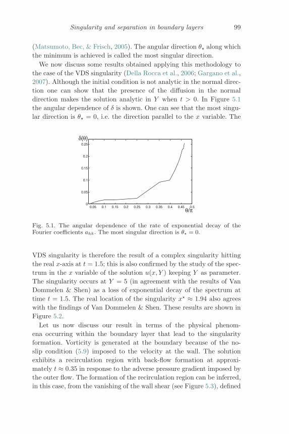
Singularity and separation in boundary layers 99
(Matsumoto, Bec, & Frisch, 2005). The angular direction θ� along whichthe minimum is achieved is called the most singular direction.
We now discuss some results obtained applying this methodology tothe case of the VDS singularity (Della Rocca et al., 2006; Gargano et al.,2007). Although the initial condition is not analytic in the normal direc-tion one can show that the presence of the diffusion in the normaldirection makes the solution analytic in Y when t > 0. In Figure 5.1the angular dependence of δ is shown. One can see that the most singu-lar direction is θ� = 0, i.e. the direction parallel to the x variable. The
0.05 0.1 0.15 0.2 0.25 0.3 0.35 0.4 0.45 0.50
0.05
0.1
0.15
0.2
0.25
θ/π
δ(θ)
Fig. 5.1. The angular dependence of the rate of exponential decay of theFourier coefficients ahk. The most singular direction is θ� = 0.
VDS singularity is therefore the result of a complex singularity hittingthe real x-axis at t = 1.5; this is also confirmed by the study of the spec-trum in the x variable of the solution u(x, Y ) keeping Y as parameter.The singularity occurs at Y = 5 (in agreement with the results of VanDommelen & Shen) as a loss of exponential decay of the spectrum attime t = 1.5. The real location of the singularity x� ≈ 1.94 also agreeswith the findings of Van Dommelen & Shen. These results are shown inFigure 5.2.
Let us now discuss our result in terms of the physical phenom-ena occurring within the boundary layer that lead to the singularityformation. Vorticity is generated at the boundary because of the no-slip condition (5.9) imposed to the velocity at the wall. The solutionexhibits a recirculation region with back-flow formation at approxi-mately t ≈ 0.35 in response to the adverse pressure gradient imposed bythe outer flow. The formation of the recirculation region can be inferred,in this case, from the vanishing of the wall shear (see Figure 5.3), defined
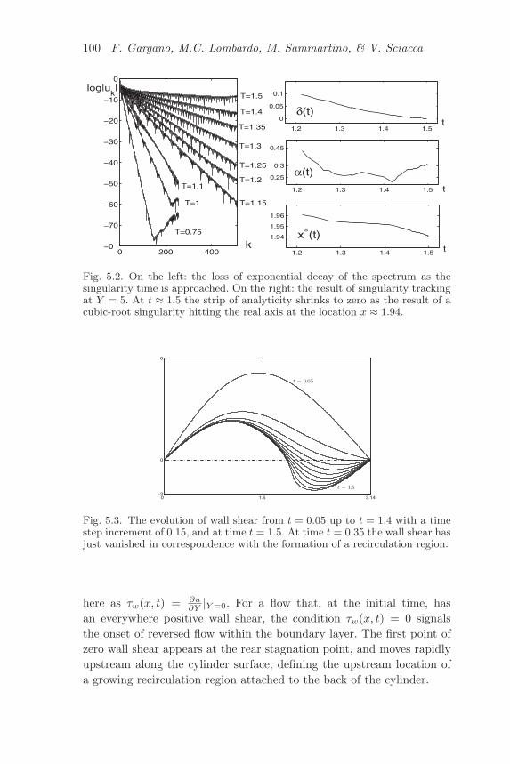
100 F. Gargano, M.C. Lombardo, M. Sammartino, & V. Sciacca
0 200 400−80
−70
−60
−50
−40
−30
−20
−10
0
1.2 1.3 1.4 1.5
0
0.05
0.1
1.2 1.3 1.4 1.5
0.3
0.45
0.25
1.2 1.3 1.4 1.5
1.94
1.95
1.96
x∗(t)
δ(t)
α(t)
t
t
t
log|uk|
kT=0.75
T=1
T=1.1
T=1.15
T=1.2
T=1.25
T=1.3
T=1.35
T=1.4
T=1.5
Fig. 5.2. On the left: the loss of exponential decay of the spectrum as thesingularity time is approached. On the right: the result of singularity trackingat Y = 5. At t ≈ 1.5 the strip of analyticity shrinks to zero as the result of acubic-root singularity hitting the real axis at the location x ≈ 1.94.
0 1.5 3.14−2
6
0
t
t
Fig. 5.3. The evolution of wall shear from t = 0.05 up to t = 1.4 with a timestep increment of 0.15, and at time t = 1.5. At time t = 0.35 the wall shear hasjust vanished in correspondence with the formation of a recirculation region.
here as τw(x, t) = ∂u∂Y |Y =0. For a flow that, at the initial time, has
an everywhere positive wall shear, the condition τw(x, t) = 0 signalsthe onset of reversed flow within the boundary layer. The first point ofzero wall shear appears at the rear stagnation point, and moves rapidlyupstream along the cylinder surface, defining the upstream location ofa growing recirculation region attached to the back of the cylinder.
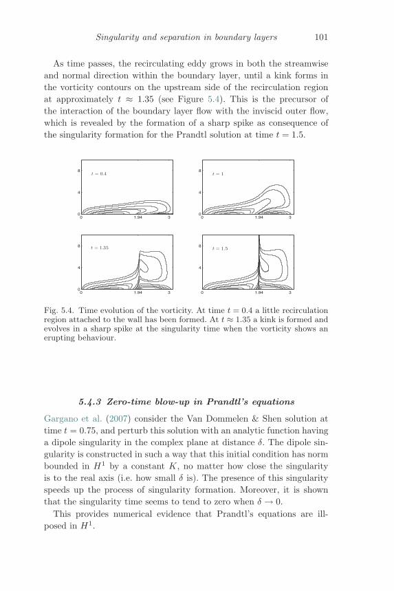
Singularity and separation in boundary layers 101
As time passes, the recirculating eddy grows in both the streamwiseand normal direction within the boundary layer, until a kink forms inthe vorticity contours on the upstream side of the recirculation regionat approximately t ≈ 1.35 (see Figure 5.4). This is the precursor ofthe interaction of the boundary layer flow with the inviscid outer flow,which is revealed by the formation of a sharp spike as consequence ofthe singularity formation for the Prandtl solution at time t = 1.5.
0 1.94 30
4
8
0 1.94 30
4
8
0 31.940
4
8
0 31.94
4
8
t t = 1
t t
Fig. 5.4. Time evolution of the vorticity. At time t = 0.4 a little recirculationregion attached to the wall has been formed. At t ≈ 1.35 a kink is formed andevolves in a sharp spike at the singularity time when the vorticity shows anerupting behaviour.
5.4.3 Zero-time blow-up in Prandtl’s equations
Gargano et al. (2007) consider the Van Dommelen & Shen solution attime t = 0.75, and perturb this solution with an analytic function havinga dipole singularity in the complex plane at distance δ. The dipole sin-gularity is constructed in such a way that this initial condition has normbounded in H1 by a constant K, no matter how close the singularityis to the real axis (i.e. how small δ is). The presence of this singularityspeeds up the process of singularity formation. Moreover, it is shownthat the singularity time seems to tend to zero when δ → 0.
This provides numerical evidence that Prandtl’s equations are ill-posed in H1.
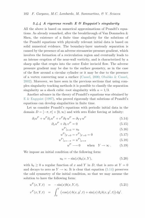
102 F. Gargano, M.C. Lombardo, M. Sammartino, & V. Sciacca
5.4.4 A rigorous result: E & Engquist’s singularity
All the above is based on numerical approximations of Prandtl’s equa-tions. As already remarked, after the breakthrough of Van Dommelen &Shen, the existence of a finite time singularity for the solutions ofthe Prandtl equations with physically relevant initial data is based onsolid numerical evidence. The boundary-layer unsteady separation iscaused by the presence of an adverse streamwise pressure gradient, whichinvolves the formation of a recirculation region and eventually leads toan intense eruption of the near-wall vorticity, and is characterized by asharp spike that erupts into the outer Euler inviscid flow. The adversepressure gradient may be due to the surface geometry, as in the caseof the flow around a circular cylinder or it may be due to the presenceof a vortex convecting near a surface (Cassel, 2000; Obabko & Cassel,2002). Moreover, we have seen in the previous sections that using com-plex singularity tracking methods it is possible to classify the separationsingularity as a shock cubic–root singularity with α = 1/3.
Another advance in the theory of Prandtl’s equations was obtained byE & Engquist (1997), who proved rigorously that solutions of Prandtl’sequations can develop singularities in finite time.
Let us consider Prandtl’s equations with periodic initial data in thedomain D = [−π, π] × [0,∞) and with zero Euler forcing at infinity:
∂tuP + uP∂xu
P + vP∂Y uP = ∂Y Y u
P (5.14)
∂xuP + ∂Y v
P = 0 (5.15)
uP |t=0 = u0 (5.16)
uP |Y =0 = vP |Y =0 = 0 (5.17)
uP |x=−π = uP |x=π (5.18)
uP −→ 0 when Y → ∞ . (5.19)
We impose an initial condition of the following form:
u0 = − sin(x)b0(x, Y ), (5.20)
with b0 ≥ 0 a regular function of x and Y in D, that is zero at Y = 0and decays to zero as Y → ∞. It is clear that equation (5.14) preservesthe odd symmetry of the initial condition, so that we may assume thesolution to have the following form:
uP (x, Y, t) = − sin(x)b(x, Y, t), (5.21)
vP (x, Y, t) =∫ Y
0
(cos(x) b(x, y′, t) + sin(x) ∂xb(x, y′, t)
)dy′.
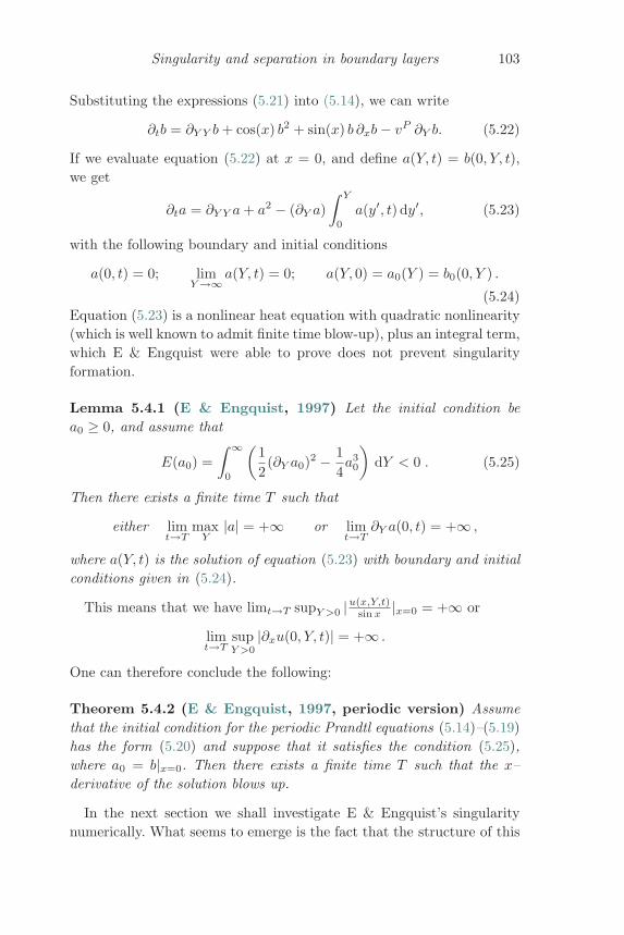
Singularity and separation in boundary layers 103
Substituting the expressions (5.21) into (5.14), we can write
∂tb = ∂Y Y b+ cos(x) b2 + sin(x) b ∂xb− vP ∂Y b. (5.22)
If we evaluate equation (5.22) at x = 0, and define a(Y, t) = b(0, Y, t),we get
∂ta = ∂Y Y a+ a2 − (∂Y a)∫ Y
0
a(y′, t) dy′, (5.23)
with the following boundary and initial conditions
a(0, t) = 0; limY →∞
a(Y, t) = 0; a(Y, 0) = a0(Y ) = b0(0, Y ) .
(5.24)Equation (5.23) is a nonlinear heat equation with quadratic nonlinearity(which is well known to admit finite time blow-up), plus an integral term,which E & Engquist were able to prove does not prevent singularityformation.
Lemma 5.4.1 (E & Engquist, 1997) Let the initial condition bea0 ≥ 0, and assume that
E(a0) =∫ ∞
0
(12
(∂Y a0)2 − 14a30
)dY < 0 . (5.25)
Then there exists a finite time T such that
either limt→T
maxY
|a| = +∞ or limt→T
∂Y a(0, t) = +∞ ,
where a(Y, t) is the solution of equation (5.23) with boundary and initialconditions given in (5.24).
This means that we have limt→T supY >0 |u(x,Y,t)sin x |x=0 = +∞ or
limt→T
supY >0
|∂xu(0, Y, t)| = +∞ .
One can therefore conclude the following:
Theorem 5.4.2 (E & Engquist, 1997, periodic version) Assumethat the initial condition for the periodic Prandtl equations (5.14)–(5.19)has the form (5.20) and suppose that it satisfies the condition (5.25),where a0 = b|x=0. Then there exists a finite time T such that the x–derivative of the solution blows up.
In the next section we shall investigate E & Engquist’s singularitynumerically. What seems to emerge is the fact that the structure of this
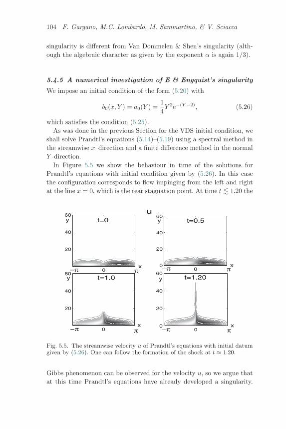
104 F. Gargano, M.C. Lombardo, M. Sammartino, & V. Sciacca
singularity is different from Van Dommelen & Shen’s singularity (alth-ough the algebraic character as given by the exponent α is again 1/3).
5.4.5 A numerical investigation of E & Engquist’s singularity
We impose an initial condition of the form (5.20) with
b0(x, Y ) = a0(Y ) =14Y 2e−(Y −2), (5.26)
which satisfies the condition (5.25).As was done in the previous Section for the VDS initial condition, we
shall solve Prandtl’s equations (5.14)–(5.19) using a spectral method inthe streamwise x–direction and a finite difference method in the normalY -direction.
In Figure 5.5 we show the behaviour in time of the solutions forPrandtl’s equations with initial condition given by (5.26). In this casethe configuration corresponds to flow impinging from the left and rightat the line x = 0, which is the rear stagnation point. At time t � 1.20 the
0
40
20
60
0
20
40
60
00
20
40
600
0
20
40
60
π
π
π
π
t=0.5
t=1.20t=1.0
t=0u
x
y
y
y
y
xx
x
−π −π
−π −π
Fig. 5.5. The streamwise velocity u of Prandtl’s equations with initial datumgiven by (5.26). One can follow the formation of the shock at t ≈ 1.20.
Gibbs phenomenon can be observed for the velocity u, so we argue thatat this time Prandtl’s equations have already developed a singularity.
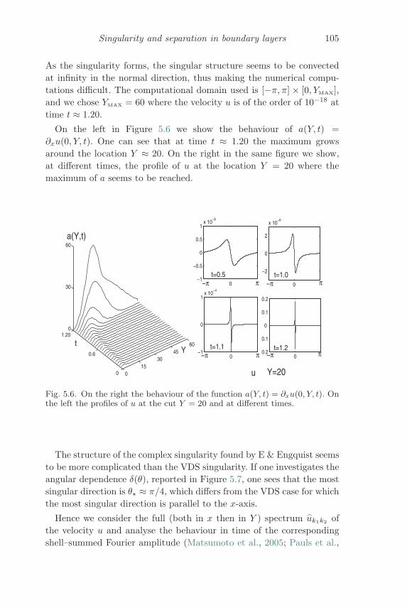
Singularity and separation in boundary layers 105
As the singularity forms, the singular structure seems to be convectedat infinity in the normal direction, thus making the numerical compu-tations difficult. The computational domain used is [−π, π] × [0, YMAX],and we chose YMAX = 60 where the velocity u is of the order of 10−18 attime t ≈ 1.20.
On the left in Figure 5.6 we show the behaviour of a(Y, t) =∂xu(0, Y, t). One can see that at time t ≈ 1.20 the maximum growsaround the location Y ≈ 20. On the right in the same figure we show,at different times, the profile of u at the location Y = 20 where themaximum of a seems to be reached.
0−1
−0.5
0
0.5
1x 10
−6
0 15
3045
60
0
0.6
1.200
30
60
00.2
0.1
0
0.1
0.2
0
−2
0
2
x 10−6
0−1
0
1x 10
−4
a(Y,t)
Yt
π−π
t=1.2t=1.1
t=1.0t=0.5
u
−π
−π
−π
π
ππ
Y=20
Fig. 5.6. On the right the behaviour of the function a(Y, t) = ∂xu(0, Y, t). Onthe left the profiles of u at the cut Y = 20 and at different times.
The structure of the complex singularity found by E & Engquist seemsto be more complicated than the VDS singularity. If one investigates theangular dependence δ(θ), reported in Figure 5.7, one sees that the mostsingular direction is θ� ≈ π/4, which differs from the VDS case for whichthe most singular direction is parallel to the x-axis.
Hence we consider the full (both in x then in Y ) spectrum uk1k2 ofthe velocity u and analyse the behaviour in time of the correspondingshell–summed Fourier amplitude (Matsumoto et al., 2005; Pauls et al.,
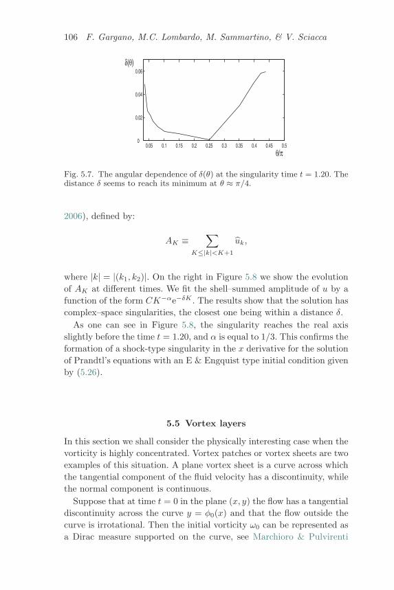
106 F. Gargano, M.C. Lombardo, M. Sammartino, & V. Sciacca
0.05 0.1 0.15 0.2 0.25 0.3 0.35 0.4 0.45 0.50
0.02
0.04
0.06δ(θ)
θ/π
Fig. 5.7. The angular dependence of δ(θ) at the singularity time t = 1.20. Thedistance δ seems to reach its minimum at θ ≈ π/4.
2006), defined by:
AK ≡∑
K≤|k|<K+1
uk,
where |k| = |(k1, k2)|. On the right in Figure 5.8 we show the evolutionof AK at different times. We fit the shell–summed amplitude of u by afunction of the form CK−αe−δK . The results show that the solution hascomplex–space singularities, the closest one being within a distance δ.
As one can see in Figure 5.8, the singularity reaches the real axisslightly before the time t = 1.20, and α is equal to 1/3. This confirms theformation of a shock-type singularity in the x derivative for the solutionof Prandtl’s equations with an E & Engquist type initial condition givenby (5.26).
5.5 Vortex layers
In this section we shall consider the physically interesting case when thevorticity is highly concentrated. Vortex patches or vortex sheets are twoexamples of this situation. A plane vortex sheet is a curve across whichthe tangential component of the fluid velocity has a discontinuity, whilethe normal component is continuous.
Suppose that at time t = 0 in the plane (x, y) the flow has a tangentialdiscontinuity across the curve y = φ0(x) and that the flow outside thecurve is irrotational. Then the initial vorticity ω0 can be represented asa Dirac measure supported on the curve, see Marchioro & Pulvirenti
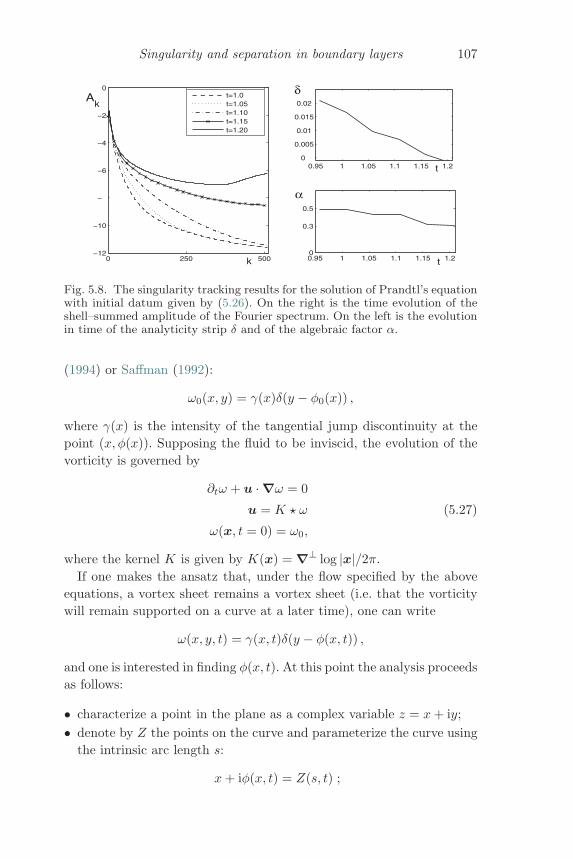
Singularity and separation in boundary layers 107
0 250 500−12
−10
−8
−6
−4
−2
0
0.95 1 1.05 1.1 1.15 1.20
0.005
0.01
0.015
0.02
0.95 1 1.05 1.1 1.15 1.20
0.5
0.3
t=1.0t=1.05t=1.10t=1.15t=1.20
k
Ak
t
α
δ
t
Fig. 5.8. The singularity tracking results for the solution of Prandtl’s equationwith initial datum given by (5.26). On the right is the time evolution of theshell–summed amplitude of the Fourier spectrum. On the left is the evolutionin time of the analyticity strip δ and of the algebraic factor α.
(1994) or Saffman (1992):
ω0(x, y) = γ(x)δ(y − φ0(x)) ,
where γ(x) is the intensity of the tangential jump discontinuity at thepoint (x, φ(x)). Supposing the fluid to be inviscid, the evolution of thevorticity is governed by
∂tω + u · ∇ω = 0
u = K � ω (5.27)
ω(x, t = 0) = ω0,
where the kernel K is given by K(x) = ∇⊥ log |x|/2π.If one makes the ansatz that, under the flow specified by the above
equations, a vortex sheet remains a vortex sheet (i.e. that the vorticitywill remain supported on a curve at a later time), one can write
ω(x, y, t) = γ(x, t)δ(y − φ(x, t)) ,
and one is interested in finding φ(x, t). At this point the analysis proceedsas follows:
• characterize a point in the plane as a complex variable z = x+ iy;• denote by Z the points on the curve and parameterize the curve using
the intrinsic arc length s:
x+ iφ(x, t) = Z(s, t) ;
108 F. Gargano, M.C. Lombardo, M. Sammartino, & V. Sciacca
• use (5.27) to write:
u(z, t) − iv(z, t) = − i2π
∫γ(s′, t)
z − Z(s′, t)ds′ ;
• using the above formula write the velocity of the sheet (U, V ) as theprincipal value of the integral:
U(s, t) − iV (s, t) ≡ ∂Z
∂t= − i
2πPV
∫γ(s′, t)
Z(s, t) − Z(s′, t)ds′ ;
• finally, parameterize the curve using the total circulation Γ(s, t)contained between a reference point Z(s∗, t) and the generic pointZ(s, t):
∂Z
∂t= − i
2πPV
∫dΓ′
Z(Γ, t) − Z(Γ′, t).
The above equation is the Birkhoff–Rott equation, which has been exten-sively studied from the mathematical point of view as well as from thenumerical one.
The Birkhoff–Rott equation develops a singularity, which first man-ifests itself as an infinite curvature (a cusp) in the shape of the sheet.Moreover, the singularity time can be made short, thus making theBirkhoff–Rott equation an ill–posed problem. This was found usingasymptotic methods by Moore (1979), verified numerically by Krasny(1986), and proved rigorously by Caflisch & Orellana (1986).
On the other hand it was proved by Sulem et al. (1981) that, if theinitial condition has an exponentially decaying Fourier spectrum, thenone has local-in-time existence and uniqueness of the solution. One canachieve long-time existence for small enough perturbations of the flatsheet (Caflisch & Orellana, 1986) or taking into account the regularizingeffect of the surface tension (Hou, Lowengrub, & Shelley, 1997).
A different kind of regularization has been recently achieved in Bardos,Linshiz, & Titi (2008) using the 2D Euler-α equations instead of theEuler equations. The Euler–α equations are
∂tω + u · ∇ω = 0
u = Kα � ω
ω(x, t = 0) = ω0,
where Kα = Gα � K with Gα a regularizing kernel that has symbol(1 + α2|k|2)−1, and k is the dual Fourier variable of x.
Singularity and separation in boundary layers 109
The fact that the Birkhoff–Rott–α model has a better behaviour thanthe usual Birkhoff–Rott equations can be understood by studying thelinear stability of the flat sheet. In this case it is more convenient tostart with the equations
∂tφ = −u1∂xφ+ u2
∂tγ = −γ∂xu1 − u1∂xγ
(Marchioro & Pulvirenti, 1994). Denoting by φ, (u1, u2), and γ the(small) deviations from a flat sheet with constant jump intensity γ0,one derives the linear system
∂tφ = u2
∂tγ = −γ0∂xu1 .
If one passes to the Fourier representation and uses the fact that thevelocity is governed by the Euler–α equations, one can show that theabove system admits a positive eigenvalue λ(k),
λ(k) =12|γ0||k|
[1 −
(α2k2
1 + α2k2
)1/2],
which however decays to zero like 1/(α2k) as k → ∞. This has to becontrasted with the usual Birkhoff–Rott behaviour (which can be recov-ered from the above equation when α = 0) which gives a linear growthwith k of the positive eigenvalue. It is this growth which, ultimately, isthe origin of the ill–posed behaviour of the Birkhoff–Rott equations.
A different line of thought, which we shall not review here, is basedon the analysis of the vortex sheet data in terms of measure solutions ofthe Euler equations. The reader can consult the papers by Delort (1991),Majda (1993), Evans & Muller (1994), Schochet (1996), and Lopes Filho,Nussenzveig Lopes, & Schochet (2007), and references therein.
5.5.1 Vortex layers
From the physical point of view, it is clear that the most natural kindof regularization to be considered is viscous regularization. If a smallviscosity is present the vorticity would be spread out. Even initially ifit is highly concentrated on a curve, after a small time τ the vorticitywould stay on a layer of thickness
√ντ . A vortex sheet is therefore an
approximation of a vortex layer and the main mathematical questionregarding this model is to know if, when the viscosity is small, a vortex
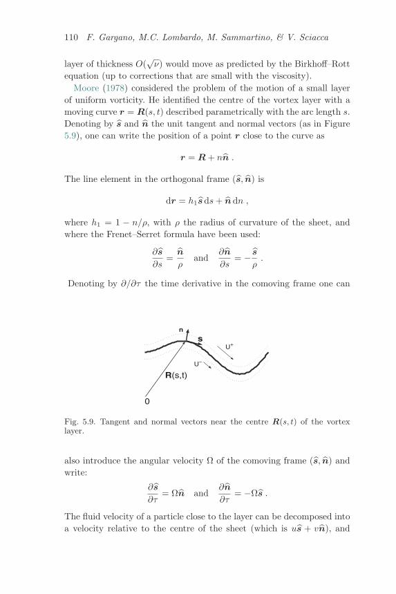
110 F. Gargano, M.C. Lombardo, M. Sammartino, & V. Sciacca
layer of thickness O(√ν) would move as predicted by the Birkhoff–Rott
equation (up to corrections that are small with the viscosity).Moore (1978) considered the problem of the motion of a small layer
of uniform vorticity. He identified the centre of the vortex layer with amoving curve r = R(s, t) described parametrically with the arc length s.Denoting by s and n the unit tangent and normal vectors (as in Figure5.9), one can write the position of a point r close to the curve as
r = R + nn .
The line element in the orthogonal frame (s, n) is
dr = h1s ds+ n dn ,
where h1 = 1 − n/ρ, with ρ the radius of curvature of the sheet, andwhere the Frenet–Serret formula have been used:
∂s
∂s=
n
ρand
∂n
∂s= − s
ρ.
Denoting by ∂/∂τ the time derivative in the comoving frame one can
U+
U−
0
n
s
R(s,t)
Fig. 5.9. Tangent and normal vectors near the centre R(s, t) of the vortexlayer.
also introduce the angular velocity Ω of the comoving frame (s, n) andwrite:
∂s
∂τ= Ωn and
∂n
∂τ= −Ωs .
The fluid velocity of a particle close to the layer can be decomposed intoa velocity relative to the centre of the sheet (which is us + vn), and
Singularity and separation in boundary layers 111
a part due to the motion of the sheet (which is ∂τR + n∂τ n):
U = [u+ ∂τX − Ω(Y + n)] s + [v + ∂τY + ΩX] n . (5.28)
In the above equation, by X and Y we have denoted the components ofR (the vector giving the centre of the sheet) in the intrinsic coordinatesystem, i.e. R = Xs + Y n.
Moore supposed that the vorticity is uniformly distributed in a smalllayer surrounding the curve of thickness 2H = O(ε), while it is zerooutside this layer. Moreover he assumed that the radius of curvatureis uniformly much larger than the thickness of the layer, specificallyH ≤ ρε. Introducing the rescaled normal variable
N =n
ε, (5.29)
and expanding the velocity field as:
u(s, n, t) = u0(s, n, t) + εu1(s, n, t) + ε2u2(s, n, t) + . . . (5.30)
v(s, n, t) = εv0(s, n, t) + ε2v1(s, n, t) + . . . , (5.31)
Moore performed an asymptotic matching procedure between the outerflow and the inner flow and obtained the following equation for themotion of the centre of the sheet:
∂Z∗
∂t= − i
2πPV
∫dΓ′
Z(Γ, t) − Z(Γ′, t)− ε
i6ω
∂
∂Γ
(G4 ∂Z
∗
∂Γ
)+O(ε2) ,
(5.32)
which contains an O(ε) correction to the Birkhoff–Rott equation. In(5.32), G denotes the quantity γ(s, t) expressed in terms of the variableΓ, and ω = O(1) denotes the rescaled constant vorticity of the layer.
Later, Benedetto & Pulvirenti (1992) proved rigorously, in an analyticfunction space, that the Euler dynamics of a layer of constant vortic-ity converges to the dynamics of the Birkhoff–Rott equation when thethickness of the layer goes to zero.
Clearly, assuming that vorticity is a constant inside the layer does notdescribe correctly the smoothing effects of the viscosity. Later Dhanak(1994a,b) derived an interesting generalization of Moore’s equation. Hetook into account the role of the viscosity ν and assumed that the vor-ticity, not supposed uniform, decays exponentially fast away from thecentre of the sheet,
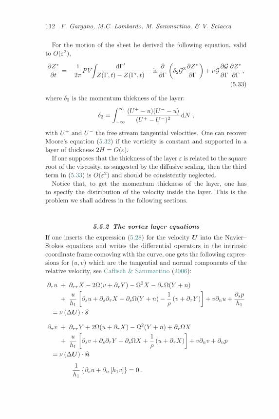
112 F. Gargano, M.C. Lombardo, M. Sammartino, & V. Sciacca
For the motion of the sheet he derived the following equation, validto O(ε2),
∂Z∗
∂t= − i
2πPV
∫dΓ′
Z(Γ, t) − Z(Γ′, t)− iε
∂
∂Γ
(δ2G3 ∂Z
∗
∂Γ
)+ νG ∂G
∂Γ∂Z∗
∂Γ,
(5.33)
where δ2 is the momentum thickness of the layer:
δ2 =∫ ∞
−∞
(U+ − u)(U− − u)(U+ − U−)2
dN ,
with U+ and U− the free stream tangential velocities. One can recoverMoore’s equation (5.32) if the vorticity is constant and supported in alayer of thickness 2H = O(ε).
If one supposes that the thickness of the layer ε is related to the squareroot of the viscosity, as suggested by the diffusive scaling, then the thirdterm in (5.33) is O(ε2) and should be consistently neglected.
Notice that, to get the momentum thickness of the layer, one hasto specify the distribution of the velocity inside the layer. This is theproblem we shall address in the following sections.
5.5.2 The vortex layer equations
If one inserts the expression (5.28) for the velocity U into the Navier–Stokes equations and writes the differential operators in the intrinsiccoordinate frame comoving with the curve, one gets the following expres-sions for (u, v) which are the tangential and normal components of therelative velocity, see Caflisch & Sammartino (2006):
∂τu + ∂ττX − 2Ω(v + ∂τY ) − Ω2X − ∂τ Ω(Y + n)
+u
h1
[∂su+ ∂s∂τX − ∂sΩ(Y + n) − 1
ρ(v + ∂τY )
]+ v∂nu+
∂sp
h1
= ν (ΔU) · s
∂τv + ∂ττY + 2Ω(u+ ∂τX) − Ω2(Y + n) + ∂τ ΩX
+u
h1
[∂sv + ∂s∂τY + ∂sΩX +
1ρ
(u+ ∂τX)]
+ v∂nv + ∂np
= ν (ΔU) · n1h1
{∂su+ ∂n [h1v]} = 0 .
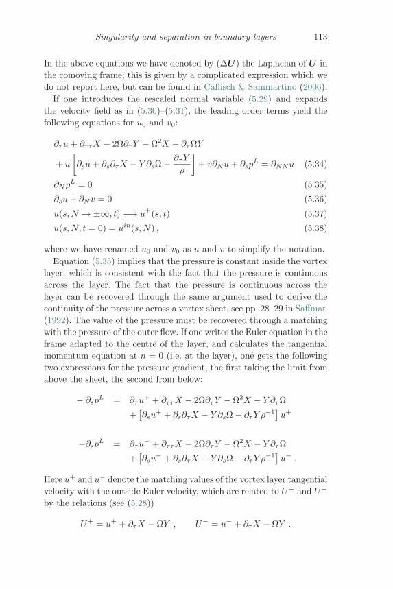
Singularity and separation in boundary layers 113
In the above equations we have denoted by (ΔU) the Laplacian of U inthe comoving frame; this is given by a complicated expression which wedo not report here, but can be found in Caflisch & Sammartino (2006).
If one introduces the rescaled normal variable (5.29) and expandsthe velocity field as in (5.30)–(5.31), the leading order terms yield thefollowing equations for u0 and v0:
∂τu+ ∂ττX − 2Ω∂τY − Ω2X − ∂τ ΩY
+ u
[∂su+ ∂s∂τX − Y ∂sΩ − ∂τY
ρ
]+ v∂Nu+ ∂sp
L = ∂NNu (5.34)
∂NpL = 0 (5.35)
∂su+ ∂Nv = 0 (5.36)
u(s,N → ±∞, t) −→ u±(s, t) (5.37)
u(s,N, t = 0) = uin(s,N) , (5.38)
where we have renamed u0 and v0 as u and v to simplify the notation.Equation (5.35) implies that the pressure is constant inside the vortex
layer, which is consistent with the fact that the pressure is continuousacross the layer. The fact that the pressure is continuous across thelayer can be recovered through the same argument used to derive thecontinuity of the pressure across a vortex sheet, see pp. 28–29 in Saffman(1992). The value of the pressure must be recovered through a matchingwith the pressure of the outer flow. If one writes the Euler equation in theframe adapted to the centre of the layer, and calculates the tangentialmomentum equation at n = 0 (i.e. at the layer), one gets the followingtwo expressions for the pressure gradient, the first taking the limit fromabove the sheet, the second from below:
− ∂spL = ∂τu
+ + ∂ττX − 2Ω∂τY − Ω2X − Y ∂τ Ω
+[∂su
+ + ∂s∂τX − Y ∂sΩ − ∂τY ρ−1]u+
−∂spL = ∂τu
− + ∂ττX − 2Ω∂τY − Ω2X − Y ∂τ Ω
+[∂su
− + ∂s∂τX − Y ∂sΩ − ∂τY ρ−1]u− .
Here u+ and u− denote the matching values of the vortex layer tangentialvelocity with the outside Euler velocity, which are related to U+ and U−
by the relations (see (5.28))
U+ = u+ + ∂τX − ΩY , U− = u− + ∂τX − ΩY .
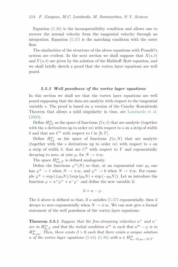
114 F. Gargano, M.C. Lombardo, M. Sammartino, & V. Sciacca
Equation (5.36) is the incompressibility condition and allows one torecover the normal velocity from the tangential velocity through anintegration. Equation (5.37) is the matching condition with the outerflow.
The similarities of the structure of the above equations with Prandtl’ssystem are evident. In the next section we shall suppose that X(s, t)and Y (s, t) are given by the solution of the Birkhoff–Rott equation, andwe shall briefly sketch a proof that the vortex layer equations are wellposed.
5.5.3 Well posedness of the vortex layer equations
In this section we shall see that the vortex layer equations are wellposed supposing that the data are analytic with respect to the tangentialvariable s. The proof is based on a version of the Cauchy–KowalewskiTheorem that allows a mild singularity in time, see Lombardo et al.(2003).
Define Hmδ,T as the space of functions f(s, t) that are analytic (together
with the s derivatives up to order m) with respect to s on a strip of widthδ and that are C1 with respect to t in [0, T ].
Define Hmδ,μ as the space of functions f(s,N) that are analytic
(together with the s derivatives up to order m) with respect to s ona strip of width δ, that are C2 with respect to Y and exponentiallydecaying to zero, at rate μ, for N → ±∞.
The space Hmδ,μ,T is defined analogously.
Define the functions ϕ±(N) so that, at an exponential rate μ0 onehas ϕ± → 1 when N → ±∞, and ϕ± → 0 when N → ∓∞. For exam-ple ϕ± = exp (±μ0N)/(exp (μ0N) + exp (−μ0N)). Let us introduce thefunction ϕ = u+ϕ+ + u−ϕ− and define the new variable u:
u = u− ϕ .
The u above is defined so that, if u satisfies (5.37) exponentially, then udecays to zero exponentially when N → ±∞. We can now give a formalstatement of the well posedness of the vortex layer equations:
Theorem 5.5.1 Suppose that the free-streaming velocities u+ and u−
are in Hmδ0,T and that the initial condition uin is such that uin −ϕ is in
Hmδ0,μ0
. Then, there exists β > 0 such that there exists a unique solutionu of the vortex layer equations (5.34)–(5.38) with u ∈ Hm
δ0−βt,μ0−βt,T .
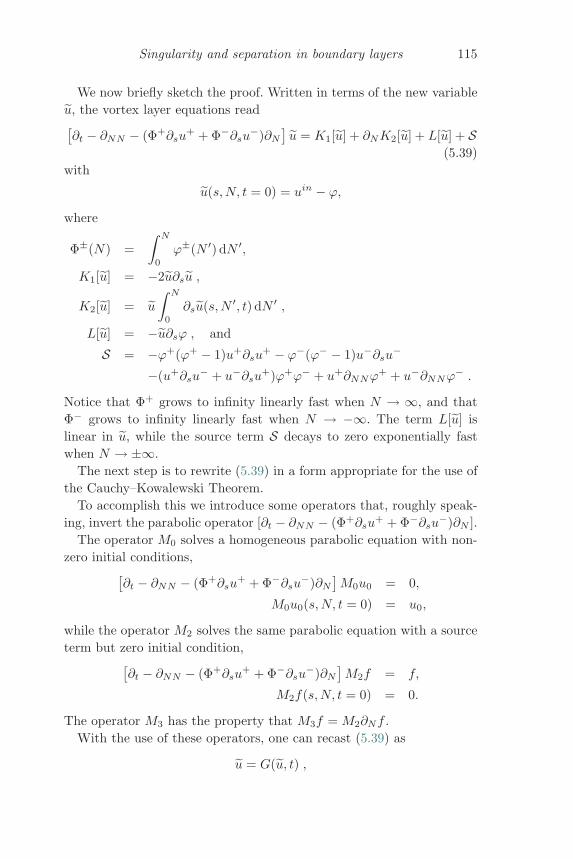
Singularity and separation in boundary layers 115
We now briefly sketch the proof. Written in terms of the new variableu, the vortex layer equations read[∂t − ∂NN − (Φ+∂su
+ + Φ−∂su−)∂N
]u = K1[u] + ∂NK2[u] + L[u] + S
(5.39)with
u(s,N, t = 0) = uin − ϕ,
where
Φ±(N) =∫ N
0
ϕ±(N ′) dN ′,
K1[u] = −2u∂su ,
K2[u] = u
∫ N
0
∂su(s,N ′, t) dN ′ ,
L[u] = −u∂sϕ , and
S = −ϕ+(ϕ+ − 1)u+∂su+ − ϕ−(ϕ− − 1)u−∂su
−
−(u+∂su− + u−∂su
+)ϕ+ϕ− + u+∂NNϕ+ + u−∂NNϕ
− .
Notice that Φ+ grows to infinity linearly fast when N → ∞, and thatΦ− grows to infinity linearly fast when N → −∞. The term L[u] islinear in u, while the source term S decays to zero exponentially fastwhen N → ±∞.
The next step is to rewrite (5.39) in a form appropriate for the use ofthe Cauchy–Kowalewski Theorem.
To accomplish this we introduce some operators that, roughly speak-ing, invert the parabolic operator [∂t − ∂NN − (Φ+∂su
+ + Φ−∂su−)∂N ].
The operator M0 solves a homogeneous parabolic equation with non-zero initial conditions,[
∂t − ∂NN − (Φ+∂su+ + Φ−∂su
−)∂N
]M0u0 = 0,
M0u0(s,N, t = 0) = u0,
while the operator M2 solves the same parabolic equation with a sourceterm but zero initial condition,[
∂t − ∂NN − (Φ+∂su+ + Φ−∂su
−)∂N
]M2f = f,
M2f(s,N, t = 0) = 0.
The operator M3 has the property that M3f = M2∂Nf .With the use of these operators, one can recast (5.39) as
u = G(u, t) ,
116 F. Gargano, M.C. Lombardo, M. Sammartino, & V. Sciacca
where
G[u, t] = M2 (K1[u] + L[u] + S) +M3K2[u] +M0 (u0 − ϕ) .
Using the Cauchy–Kowalewski Theorem, the Cauchy estimate on thederivative of an analytic function, and some estimates on the operatorsMi, the proof of the well posedness is relatively straightforward.
5.6 Concluding remarks
In this paper we have reviewed some relevant results, both numerical andtheoretical, regarding the well posedness of the boundary layer equationsin relation to the zero-viscosity limit of the Navier–Stokes equations. Inthis respect a well-established mathematical framework is still lacking,the main open problems being the following:
• In presence of a boundary, both in two and three spatial dimensions,the convergence of the solutions of the Navier–Stokes equations tothe solutions of the Euler equations for smooth initial data is still anopen question. The problem is even more striking on plane domains,where regular global solutions of both the Navier–Stokes and the Eulerequations are known to exist. If the data are analytic, then convergenceoccurs.
The study of the inviscid limit may also be complicated, even inthe absence of boundary effects, in the case of non-smooth initial datasuch as vortex patches or sheets. In this case the Birkhoff–Rott equa-tion, which governs the evolution of the vortex sheet, is an ill-posedproblem. In the case of a vortex layer of thickness O(
√ν) the equa-
tions of motion are known but their well-posedness has been provedonly in the space of analytic functions.
• Prandtl’s equations, which govern the behaviour of the fluid in aO(
√ν) neighbourhood of the boundary, are conjectured to be gen-
erally ill-posed in Sobolev spaces. In fact the existing well-posednesstheorems require either monotone or analytic (with respect to thetangential variable) data. Related to the well-posedness of Prandtl’sequations is the important mathematical problem of the finite timeblow-up of its solutions: in fact the only known theoretical result inthis direction holds for initial data with strong recirculation.
Careful numerical studies are required to investigate the above ques-tions. We have presented some recent numerical results that confirmthe development of a zero-time singularity formation (in H1) for theboundary-layer equations.
Singularity and separation in boundary layers 117
We conclude this paper with a few words about the bibliography. Thereference list, although of some length (as one would expect for a sub-ject in which many different approaches have contributed to our currentunderstanding), is far from being exhaustive. It should be consideredonly a guide for the interested reader who will find, in the cited papersand in the references therein, material for further investigation.
Acknowledgements
M. Sammartino acknowledges several interesting discussions on the vor-tex layer equations with Xinyu He. It is also a pleasure to thank JamesRobinson and Jose Rodrigo for the organization of a fantastic workshop.
This work has been supported by the INDAM and by the PRINgrant Propagazione non lineare e stabilita nei processi termodinamicidel continuo.
ReferencesAbidi, H. & Danchin, R. (2004) Optimal bounds for the inviscid limit of
Navier–Stokes equations. Asymptotic Analysis 38, no. 1, 35–46.Asano, K. (1988) Zero viscosity limit of the incompressible Navier–Stokes
equations I and II. Preprint.Bardos, C., Linshiz, J.S., & Titi, E.S. (2008) Global regularity for a Birkhoff-
Rott-α approximation of the dynamics of vortex sheets of the 2D Eulerequations, Physica D 237, 1905–1911.
Beale, J.T. & Majda, A. (1981) Rates of convergence for viscous splitting ofthe Navier–Stokes equations. Math. Comp. 37, no. 156, 243–259.
Benedetto, D. & Pulvirenti, M. (1992) From vortex layers to vortex sheets.SIAM J. Appl. Math. 52, 1041–1056.
Boyd, J.P. (2000) Chebyshev and Fourier Spectral Methods. Dover Publica-tions.
Brinckman, K.W. & Walker, J.D.A. (2001) Instability in a viscous flow drivenby streamwise vortices. J. Fluid Mech. 432, 127–166.
Caflisch, R.E. & Orellana, O.F. (1986) Long time existence for a slightlyperturbed vortex sheet. Comm. Pure Appl. Math. 39, 807–838.
Caflisch, R.E. & Sammartino, M. (2000) Existence and singularities for thePrandtl boundary layer equations. Z. Angew. Math. Mech. 80, 733-744.
Caflisch, R.E. & Sammartino, M. (2006) Vortex layers in the small viscos-ity limit, in Monaco, R., Mulone, G., Rionero, S., & Ruggeri T. (eds.)Proceedings WASCOM 2005. World Sci. Publ., Hackensack.
Cannone, M., Lombardo, M.C., & Sammartino, M. (2001) Existence anduniqueness for the Prandtl equations. C. R. Acad. Sci. Paris Ser. I Math.332, 277–282.
Carrier, F.G., Krook, M., & Pearson, C.E. (1966) Functions of a complexvariable. Theory and technique. McGraw Hill.
Cassel, K.W. (2000) A comparison of Navier–Stokes solutions with the theo-retical description of unsteady separation. Phil. Trans. R. Soc. Lond. A358, 3207–3227.
118 F. Gargano, M.C. Lombardo, M. Sammartino, & V. Sciacca
Chemetov, N.V. & Antontsev, S.N. (2008) Euler equations with non homoge-neous Navier slip boundary conditions. Physica D 237, 92–105.
Chemin, J.Y. (1996) A remark on the inviscid limit for two dimensionalincompressible fluids. Comm. Partial Differential Equations 21, 1771–1779.
Cheng, W. & Wang, X. (2007) Discrete Kato-type theorem on inviscid limitof Navier–Stokes flows. J. Math. Phys. 48, 065303.
Clopeau, T., Mikelic, A., & Robert, R. (1998) On the vanishing viscosity limitfor the 2D incompressible Navier–Stokes equations with the friction typeboundary conditions. Nonlinearity 11, 1625–1636.
Collins, W.M. & Dennis, S.C.R. (1973) Flow past an impulsively startedcircular cylinder. J. Fluid Mech. 60, 105–127.
Constantin, P. & Wu, J. (1995) Inviscid limit for vortex patches. Nonlinearity8, 735–742.
Cowley, S.J. (2001) Laminar boundary-layer theory: a 20th century paradox?in Aref, H. & Phillips, J.W. (eds.) Mechanics for a New Millennium,Proceedings of 20th ICTAM. Springer, New York.
Cozzi, E. & Kelliher, J.P. (2007) Vanishing viscosity in the plane for vorticity inborderline spaces of Besov type. J. Differential Equations 235, 647–657.
Della Rocca, G., Lombardo, M.C., Sammartino, M., & Sciacca, V. (2006)Singularity tracking for Camassa-Holm and Prandtl’s equations. Appl.Num. Math. 56, 1108–1122.
Delort, J.M. (1991) Existence de nappes de tourbillon en dimension deux. J.Amer. Math. Soc. 4, 553–586.
Dhanak, M.R. (1994a) Equation of motion of a diffusing vortex sheet. J. FluidMech. 269, 265–281.
Dhanak, M.R. (1994b) On the equation of motion of a thin layer of uniformvorticity. Stud. Appl. Math. 92, 115–125.
E, W. (2000) Boundary layer theory and the zero-viscosity limit of the Navier–Stokes equation. Acta Math. Sin. 16, no. 2, 207–218.
E, W. & Engquist, B. (1997) Blowup of solutions of the unsteady Prandtl’sequation. Comm. Pure Appl. Math. 50, no. 12, 1287–1293.
Evans, L.C. & Muller, S. (1994) Hardy spaces and the two-dimensional Eulerequations with nonnegative vorticity. J. Amer. Math. Soc. 7, 199–219.
Frisch, U., Matsumoto, T., & Bec, J. (2003) Singularities of Euler flow? Notout of the blue! J. Stat. Phys. 113, 761–781.
Gargano, F., Sammartino, M., & Sciacca, V. (2007) Singularity formation forPrandtl’s equations, submitted.
Golovkin, K.K. (1966) Vanishing viscosity in cauchy’s problem for hydrome-chanics. Trudy Mat. Inst. Steklov. 92, 31–49.
Grenier, E. (2000) On the nonlinear instability of Euler and Prandtl equations.Comm. Pure Appl. Math. 53, no. 9, 1067–1091.
Hou, T.Y., Lowengrub, J.S., & Shelley, M.J. (1997) The long-time motion ofvortex sheets with surface tension. Phys. Fluids 9, 1933–1954.
Iftimie, D. & Planas, G. (2006) Inviscid limits for the Navier–Stokesequations with Navier friction boundary conditions. Nonlinearity 19,899–918.
Jager, W. & Mikelic, A. (2001) On the roughness induced effective boundaryconditions for an incompressible viscous flow. J. Differential Equations170, 96–122.
Singularity and separation in boundary layers 119
Kato, T. (1972) Nonstationary flows of viscous and ideal fluids in R3. J. Funct.Anal. 9, 296–305.
Kato, T. (1984) Remarks on zero viscosity limit for nonstationary Navier–Stokes flows with boundary. Seminar on nonlinear partial differentialequations (Berkeley, Calif., 1983) 85–98. Springer, New York.
Kelliher, J.P. (2006) Navier–Stokes equations with Navier boundary conditionsfor a bounded domain in the plane. SIAM J. Math. Anal. 38, 210–232.
Kelliher, J.P. (2007) On Kato’s conditions for vanishing viscosity. IndianaUniv. Math. J. 56, no. 4, 1711–1721.
Krasny, R. (1986) A study of singularity formation in a vortex sheet by thepoint-vortex approximation. J. Fluid Mech. 167, 65–93.
Lions, J.L. (1969) Quelques methodes de resolutions des problemes aux limitesnon lineaires. Dunod, Gauthier–Villars, Paris.
Lombardo, M.C. (2001) Analytic solutions of the Navier–Stokes equations.Rend. Circ. Mat. Palermo 50, 299–311.
Lombardo, M.C., Cannone, M., & Sammartino, M. (2003) Well-posedness ofthe boundary layer equations. SIAM J. Math. Anal. 35, no. 4, 987–1004.
Lopes Filho, M.C. (2007) Boundary layers and the vanishing viscosity limitfor incompressible 2D flow. arXiv0712.0875v1.
Lopes Filho, M.C., Nussenzveig Lopes, H.J., & Planas, G. (2005) On theinviscid limit for 2D incompressible flow with Navier friction condition.SIAM J. Math. Anal. 36, 1130–1141.
Lopes Filho, M.C., Nussenzveig Lopes, H.J., & Schochet, S. (2007) A criterionfor the equivalence of the Birkhoff–Rott and Euler descriptions of vortexsheet evolution. Trans. Amer. Math. Soc. 359, 4125–4142.
Majda, A. (1993) Remarks on weak solutions for vortex sheets with adistinguished sign. Indiana Univ. Math. J. 42, 921–939.
Marchioro, C. & Pulvirenti, M. (1994) Mathematical theory of incompressiblenonviscous fluids. Springer–Verlag, New York.
Marsden, J.E. (1970) Nonlinear semigroups associated with the equations fora non-homogeneous fluid. University of California, Berkeley.
Masmoudi, N. (1998) The Euler limit of the Navier–Stokes equations, androtating fluids with boundary. Arch. Rational Mech. Anal. 142, 375–394.
Matsumoto, T., Bec, J., & Frisch, U. (2005) The analytic structure of 2DEuler flow at short times. Fluid Dyn. Res. 36, 221–237.
McGrath, F.J. (1968) Nonstationary plain flow of viscous and ideal fluids.Arch. Rational Mech. Anal. 27, 329–348.
Moore, D.W. (1978) The equation of motion of a vortex layer of smallthickness. Studies in Appl. Math. 58, 119–140.
Moore, D.W. (1979) The spontaneous appearance of a singularity in the shapeof an evolving vortex sheet. Proc. Roy. Soc. London Ser. A 365, 105–119.
Obabko, A.V. & Cassel, K.W. (2002) Navier–Stokes solutions of unsteadyseparation induced by a vortex. J. Fluid Mech. 465, 99–130.
Oleinik, O.A. (1967a) On the mathematical theory of boundary layer for anunsteady flow of incompressible fluid. J. Appl. Math. Mech. 30, 951–974.
Oleinik, O.A. (1967b) Solutions of the system of equations of boundary layertheory by the method of straight lines. Soviet Physics Dokl. 12, 525–528.
Oleinik, O.A. & Samokhin, V.N. (1999) Mathematical models in boundarylayer theory. Applied Mathematics and Mathematical Computation, 15,Chapman & Hall/CRC, Boca Raton, FL.
120 F. Gargano, M.C. Lombardo, M. Sammartino, & V. Sciacca
Paicu, M. (2005) Equation periodique de Navier–Stokes sans viscosite dansune direction. Comm. Partial Differential Equations 30, 1107–1140.
Pauls, W., Matsumoto, T., Frisch, U., & Bec, J. (2006) Nature of complexsingularities for the 2D Euler equation. Physica D 219, 40–59.
Saffman, P.G. (1992) Vortex dynamics. Cambridge University Press, Cam-bridge.
Safonov, M.V. (1995) The abstract Cauchy–Kovalevskaya theorem in aweighted Banach space. Comm. Pure Appl. Math. 48, 629–637.
Sammartino, M. & Caflisch, R.E. (1998a) Zero viscosity limit for analyticsolutions of the Navier–Stokes equation on a half-space I. Existence forEuler and Prandtl equations, Comm. Math. Phys. 192, 433–461.
Sammartino, M. & Caflisch, R.E. (1998b) Zero viscosity limit for analyticsolutions of the Navier–Stokes equation on a half-space II. Constructionof the Navier–Stokes solution, Comm. Math. Phys. 192, 463–491.
Schochet, S. (1996) Point-vortex method for periodic weak solutions of the 2DEuler equations. Comm. Pure Appl. Math. 49, 911–965.
Sears, W.R. & Telionis, D.P. (1975) Boundary layer separation in unsteadyflow. J. on Appl. Math. 28, 215–235.
Sulem C., Sulem, P.L., Bardos, C., & Frisch, U. (1981) Finite time analyticityfor the two and three–dimensional Kelvin–Helmholtz instability. Comm.Math. Phys. 80, 485–516.
Sulem, C., Sulem, P.L., & Frisch, U. (1983) Tracing complex singularities withspectral methods. J. Comput. Phys. 50, 138–161.
Swann, H.S.G. (1971) The convergence with vanishing viscosity of nonstation-ary Navier–Stokes flow to ideal flow in R3. Trans. Amer. Math. Soc. 157,373–397.
Temam, R. & Wang, X. (1997) On the behavior of the solutions of the Navier–Stokes equations at vanishing viscosity. Ann. Scuola Norm. Sup. Pisa Cl.Sci. 25, 807–828.
Van Dommelen, L.L. & Shen, S. (1980) The spontaneous generation of thesingularity in a separating laminar boundary layer. J. Comput. Phys. 38,125–140.
Van Dyke, M. (1975) Perturbation methods in fluid mechanics. The ParabolicPress, Stanford.
Walker, J.D.A. (1978) The boundary layer due to rectilinear vortex. Proc. R.Soc. Lond. A. 359, 167–188.
Wang, X. (2001) A Kato type theorem on zero viscosity limit of Navier–Stokesflows. Indiana Univ. Math. J. 50, 223–241.
Xin, Z. & Zhang, L. (2004) On the global existence of solutions to the Prandtl’ssystem. Adv. Math. 181, 88–133.
6
Partial regularity results for solutions of theNavier-Stokes system
Igor KukavicaDepartment of Mathematics
University of Southern CaliforniaLos Angeles, CA 90089, USA
Abstract
In this paper we provide a self-contained proof of the partial regularityresult for the Navier-Stokes system when the force satisfies f ∈ L5/3. Wedo so by estimating the size of the space-time singularities when a forcebelongs to a more general Morrey-type class and then proving that thecondition for regularity agrees with the classical condition due to Serrinwhen f ∈ L5/3.
6.1 Introduction
In this paper we address the partial regularity of solutions of the three-dimensional Navier–Stokes system
∂tu− Δu+ ∂j(uju) + ∇p = f
∇ · u = 0 (6.1)
in the whole of R3, a bounded smooth domain in R3 with Dirichletboundary conditions, or a periodic domain. Here, u and p represent theunknown velocity and the pressure in the incompressible fluid, whilethe function f stands for the external force. Given an initial conditionu(·, 0) = u0 ∈ L2, it was proven by Leray (1934) and Hopf (1951) thatthere exists a global weak solution u ∈ L∞
t L2x ∩L2
t locH1x if, for instance,
f ∈ L∞t L
2x. Such solutions satisfy the Navier–Stokes system and an
energy inequality, but they are not known to be unique and are notknown to belong to a higher regularity space L∞
t H1x ∩ L2
t locH2x. Also,
Leray and Hopf proved existence of a local strong solution u ∈ L∞t H
1x ∩
L2tH
2x if the initial data satisfies u0 ∈ H1. Strong solutions agree with
weak solutions on the common interval of existence (Serrin, 1963), butit is not known whether they can be extended to global strong solutions.For a more detailed presentation on the existence theory we refer the
Published in Partial Differential Equations and Fluid Mechanics, edited byJames C. Robinson and Jose L. Rodrigo. c© Cambridge University Press 2009.
122 I. Kukavica
reader to Constantin & Foias (1988), Fabes et al. (1972), Lemarie-Rieusset (2002), Serrin (1962, 1963), Sohr (1983), and Temam (2001).
In a series of papers Scheffer (1976a,b, 1977) took a different approachtowards regularity by estimating the size of a (possible) set S of space-time singularities for suitable weak solutions, i.e. solutions that satisfya local version of the energy inequality. For instance, he proved thatwhen f = 0, we have H5/3(S) = 0, where Ha denotes the a-dimensionalHausdorff measure. In a classical paper Caffarelli et al. (1982) provedthat P1(S) = 0 where P1 is the one-dimensional parabolic measure(in particular P1(A) ≤ H1(A) for every set A) if the force satisfiesf ∈ L5/2+δ for some δ > 0. A simpler argument leading to the sameresult was presented by Lin (1998) (see also Ladyzhenskaya & Seregin(1999) for f satisfying a Morrey-type condition with the same scalingas the Caffarelli–Kohn–Nirenberg condition f ∈ L5/2+δ). In Kukavica(2008a) we give a simple proof of the statement P1(S) = 0 with thecondition on the force f ∈ L5/3+δ for δ > 0. For other results on partialregularity, see Lemarie-Rieusset (2002), Robinson & Sadowski (2007),Struwe (1998), and Vasseur (2007).
The purpose of the present paper is three-fold. The first goal is topresent a concise and self-contained proof of the partial regularity the-orem when a force belongs to a Morrey-type space in the same scalingclass as L5/3. The second goal is to prove the partial regularity theoremfor forces in the borderline class f ∈ L5/3, the case left open in Kukavica(2008a). The third goal of the paper is to clarify the role of the energyinequality—namely to separate the proof into parts where the energyinequality is necessary and the parts where it is not.
The structure of the paper is as follows. In Section 6.2, we specifywhen (x, t) is a singular point and prove that the singular set has one-dimensional parabolic measure zero. In Sections 6.3 and 6.4, we provethat the definition of the singular set agrees with the classical one whenthe force belongs to f ∈ L5/3+δ and f ∈ L5/3 respectively. Thus Sec-tions 6.2 and 6.3 constitute a self contained proof of the partial regularityresult when f ∈ L5/3+δ, while Sections 6.2 and 6.4 contain the proof inthe case f ∈ L5/3.
6.2 Notation and the main theorem
Let D be an open, bounded, and connected subset of R3×R. We alwaysassume that (u, p) is a suitable weak solution in D by which we mean
Partial regularity results for Navier-Stokes 123
(i) u ∈ L∞t L
2x(D) ∩ L2
tH1x(D) and p ∈ L3/2(D),
(ii) f ∈ L10/7loc (D) is divergence free,
(iii) the Navier–Stokes equations (6.1) are satisfied in D in the weaksense, and(iv) the local energy inequality holds in D, i.e.∫
|u|2φ|T + 2∫∫
R3×(−∞,T ]
|∇u|2φ
≤∫∫
R3×(−∞,T ]
(|u|2(φt + Δφ) + (|u|2 + 2p)u · ∇φ+ 2(u · f)φ
)(6.2)
for all T ∈ R and all φ ∈ C∞0 (D) such that φ ≥ 0 in D. In an effort to
simplify the expressions in the paper, we will not include dx or dt in theintegrals when it is clear from the domain of integration which variablesare being integrated. Above and in the sequel, we define
LstL
qx(D) =
{u measurable in D :
‖u‖Lst Lq
x(D) =∥∥‖u(x, t)‖Lq
x
∥∥Ls
t<∞
}.
By the Gagliardo–Nirenberg inequality, (i) implies that u ∈ L10/3(D),and therefore the assumption (ii) is a natural one to guarantee that thelast integral in (6.2) exists. The assumption p ∈ L3/2(D) on the pressurecan be weakened to p ∈ Lq
tL1x(D),where q > 1 (cf. Remark 6.2.5 below).
Above and in the sequel, we write ∇ = (∂1, ∂2, ∂2). We denote byBr(x0) the standard Euclidean ball in R3 with centre x0 and radius r andabbreviate Br = Br(0). By Qr(x0, t0) = Br(x0)× [t0 − r2, t0] we denotethe parabolic cylinder in R4 labelled by the top-centre point (x0, t0) ∈ D.Also, let Q∗
r(x0, t0) = Br(x0)× [t0 − r2, t0 + r2]. For simplicity, we writeQr = Qr(0, 0) and Br = Br(0).
Let μ be a fixed universal constant (in Sections 6.3 and 6.4 it will beassumed to be sufficiently small). We write (x, t) ∈ R (and we say that(x, t) is regular) if there exists r0 > 0 such that
1r2
∫∫Qr(x,t)∩D
(|u|3 + |p|3/2) ≤ μ3 (6.3)
for all (x, t) ∈ Q∗r0
(x0, t0) and r ∈ (0, r0]. We also define S = D\R.
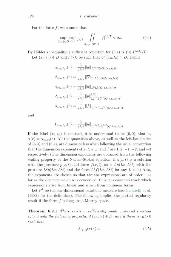
124 I. Kukavica
For the force f , we assume that
sup(x,t)∈D
supr>0
1r5/7
∫∫Qr(x,t)∩D
|f |10/7 <∞. (6.4)
By Holder’s inequality, a sufficient condition for (6.4) is f ∈ L5/3(D).Let (x0, t0) ∈ D and r > 0 be such that Qr(x0, t0) ⊆ D. Define
α(x0,t0)(r) =1r1/2
‖u‖L∞t L2
x(Qr(x0,t0)),
β(x0,t0)(r) =1r1/2
‖∇u‖L2t L2
x(Qr(x0,t0)),
γ(x0,t0)(r) =1r2/3
‖u‖L3t L3
x(Qr(x0,t0)),
δ(x0,t0)(r) =1r2/3
‖p‖1/2
L3/2t L
3/2x (Qr(x0,t0))
,
λ(x0,t0)(r) =1r1/2
‖f‖L
10/7t L
10/7x (Qr(x0,t0))
,
and
Γ(x0,t0)(r) =1r1/2
‖u‖L
10/3t L
10/3x (Qr(x0,t0))
.
If the label (x0, t0) is omitted, it is understood to be (0, 0), that is,α(r) = α(0,0)(r). All the quantities above, as well as the left-hand sidesof (6.3) and (6.4), are dimensionless when following the usual conventionthat the dimension exponents of x, t, u, p, and f are 1, 2, −1, −2, and −3respectively. (The dimension exponents are obtained from the followingscaling property of the Navier–Stokes equation: if u(x, t) is a solutionwith the pressure p(x, t) and force f(x, t), so is Lu(Lx,L2t) with thepressure L2p(Lx,L2t) and the force L3f(Lx,L2t) for any L > 0.) Also,the exponents are chosen so that the the expressions are of order 1 asfar as the dependence on u is concerned; thus it is easier to track whichexpressions arise from linear and which from nonlinear terms.
Let P1 be the one-dimensional parabolic measure (see Caffarelli et al.(1982) for the definition). The following implies the partial regularityresult if the force f belongs to a Morrey space.
Theorem 6.2.1 There exists a sufficiently small universal constantε∗ > 0 with the following property: if (x0, t0) ∈ D, and if there is r0 > 0such that
λ(x,t)(r) ≤ ε∗ (6.5)
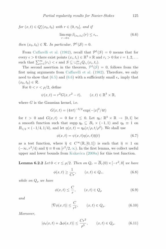
Partial regularity results for Navier-Stokes 125
for (x, t) ∈ Q∗r(x0, t0) with r ∈ (0, r0], and if
lim supr→0+
β(x0,t0)(r) ≤ ε∗, (6.6)
then (x0, t0) ∈ R. In particular, P1(S) = 0.
From Caffarelli et al. (1982), recall that P1(S) = 0 means that forevery ε > 0 there exist points (xi, ti) ∈ R3×R and ri > 0 for i = 1, 2, . . .such that
∑∞i=1(ri) < ε and S ⊆ ∪∞
i=1Qri(xi, ti).
The second assertion in the theorem, P1(S) = 0, follows from thefirst using arguments from Caffarelli et al. (1982). Therefore, we onlyneed to show that (6.5) and (6.6) with a sufficiently small ε∗ imply that(x0, t0) ∈ R.
For 0 < r < ρ/2, define
ψ(x, t) = r2G(x, r2 − t), (x, t) ∈ R3 × R,
where G is the Gaussian kernel, i.e.
G(x, t) = (4πt)−3/2 exp(−|x|2/4t)for t > 0 and G(x, t) = 0 for t ≤ 0. Let η0 : R3 × R → [0, 1] bea smooth function such that supp η0 ⊆ B1 × (−1, 1) and η0 ≡ 1 onB1/2 × (−1/4, 1/4), and let η(x, t) = η0(x/ρ, t/ρ2). We shall use
φ(x, t) = ψ(x, t)η(x, t)η(t) (6.7)
as a test function, where η ∈ C∞(R, [0, 1]) is such that η ≡ 1 on(−∞, r2/4) and η ≡ 0 on [r2/2,∞). In the first lemma, we collect usefulupper and lower bounds from Kukavica (2008a) for this test function.
Lemma 6.2.2 Let 0 < r ≤ ρ/2. Then on Qr = Br(0)× [−r2, 0] we have
φ(x, t) ≥ 1Cr
, (x, t) ∈ Qr, (6.8)
while on Qρ we have
φ(x, t) ≤ C
r, (x, t) ∈ Qρ (6.9)
and
|∇φ(x, t)| ≤ C
r2, (x, t) ∈ Qρ. (6.10)
Moreover,
|φt(x, t) + Δφ(x, t)| ≤ Cr2
ρ5, (x, t) ∈ Qρ. (6.11)
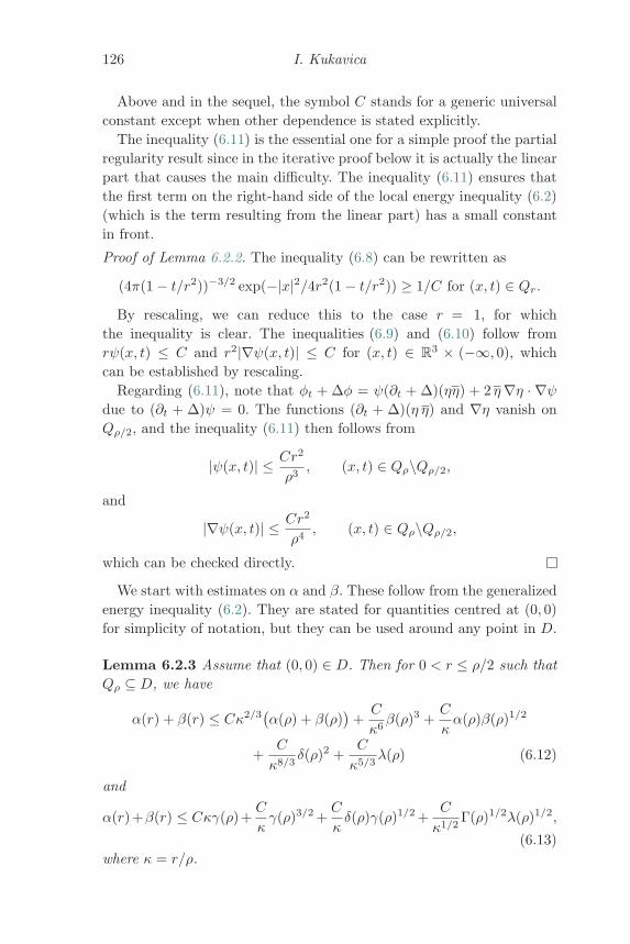
126 I. Kukavica
Above and in the sequel, the symbol C stands for a generic universalconstant except when other dependence is stated explicitly.
The inequality (6.11) is the essential one for a simple proof the partialregularity result since in the iterative proof below it is actually the linearpart that causes the main difficulty. The inequality (6.11) ensures thatthe first term on the right-hand side of the local energy inequality (6.2)(which is the term resulting from the linear part) has a small constantin front.
Proof of Lemma 6.2.2. The inequality (6.8) can be rewritten as
(4π(1 − t/r2))−3/2 exp(−|x|2/4r2(1 − t/r2)) ≥ 1/C for (x, t) ∈ Qr.
By rescaling, we can reduce this to the case r = 1, for whichthe inequality is clear. The inequalities (6.9) and (6.10) follow fromrψ(x, t) ≤ C and r2|∇ψ(x, t)| ≤ C for (x, t) ∈ R3 × (−∞, 0), whichcan be established by rescaling.
Regarding (6.11), note that φt + Δφ = ψ(∂t + Δ)(ηη) + 2 η∇η · ∇ψdue to (∂t + Δ)ψ = 0. The functions (∂t + Δ)(η η) and ∇η vanish onQρ/2, and the inequality (6.11) then follows from
|ψ(x, t)| ≤ Cr2
ρ3, (x, t) ∈ Qρ\Qρ/2,
and
|∇ψ(x, t)| ≤ Cr2
ρ4, (x, t) ∈ Qρ\Qρ/2,
which can be checked directly.
We start with estimates on α and β. These follow from the generalizedenergy inequality (6.2). They are stated for quantities centred at (0, 0)for simplicity of notation, but they can be used around any point in D.
Lemma 6.2.3 Assume that (0, 0) ∈ D. Then for 0 < r ≤ ρ/2 such thatQρ ⊆ D, we have
α(r) + β(r) ≤ Cκ2/3(α(ρ) + β(ρ)
)+C
κ6β(ρ)3 +
C
κα(ρ)β(ρ)1/2
+C
κ8/3δ(ρ)2 +
C
κ5/3λ(ρ) (6.12)
and
α(r)+β(r) ≤ Cκγ(ρ)+C
κγ(ρ)3/2 +
C
κδ(ρ)γ(ρ)1/2 +
C
κ1/2Γ(ρ)1/2λ(ρ)1/2,
(6.13)where κ = r/ρ.
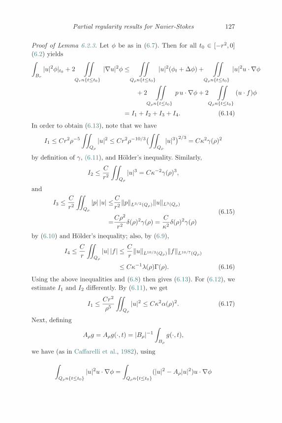
Partial regularity results for Navier-Stokes 127
Proof of Lemma 6.2.3. Let φ be as in (6.7). Then for all t0 ∈ [−r2, 0](6.2) yields∫
Br
|u|2φ|t0 + 2∫∫
Qrn{t≤t0}
|∇u|2φ ≤∫∫
Qρn{t≤t0}
|u|2(φt + Δφ) +∫∫
Qρn{t≤t0}
|u|2u · ∇φ
+ 2∫∫
Qρn{t≤t0}
p u · ∇φ+ 2∫∫
Qρn{t≤t0}
(u · f)φ
= I1 + I2 + I3 + I4. (6.14)
In order to obtain (6.13), note that we have
I1 ≤ Cr2ρ−5
∫∫Qρ
|u|2 ≤ Cr2ρ−10/3(∫∫
Qρ
|u|3)2/3 = Cκ2γ(ρ)2
by definition of γ, (6.11), and Holder’s inequality. Similarly,
I2 ≤ C
r2
∫∫Qρ
|u|3 = Cκ−2γ(ρ)3,
and
I3 ≤ C
r2
∫∫Qρ
|p| |u| ≤C
r2‖p‖L3/2(Qρ)‖u‖L3(Qρ)
=Cρ2
r2δ(ρ)2γ(ρ) =
C
κ2δ(ρ)2γ(ρ)
(6.15)
by (6.10) and Holder’s inequality; also, by (6.9),
I4 ≤ C
r
∫∫Qρ
|u| |f | ≤ C
r‖u‖L10/3(Qρ)‖f‖L10/7(Qρ)
≤ Cκ−1λ(ρ)Γ(ρ). (6.16)
Using the above inequalities and (6.8) then gives (6.13). For (6.12), weestimate I1 and I2 differently. By (6.11), we get
I1 ≤ Cr2
ρ5
∫∫Qρ
|u|2 ≤ Cκ2α(ρ)2. (6.17)
Next, defining
Aρg = Aρg(·, t) = |Bρ|−1
∫Bρ
g(·, t),
we have (as in Caffarelli et al., 1982), using∫Qρn{t≤t0}
|u|2u · ∇φ =∫
Qρn{t≤t0}(|u|2 −Aρ|u|2)u · ∇φ
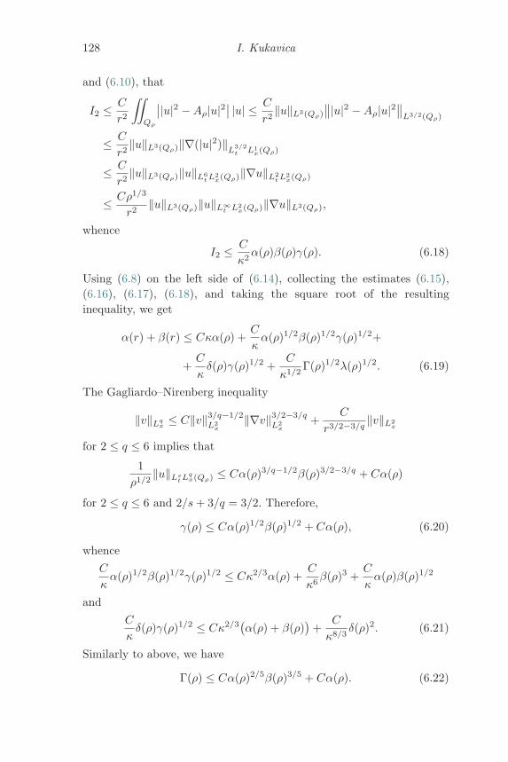
128 I. Kukavica
and (6.10), that
I2 ≤ C
r2
∫∫Qρ
∣∣|u|2 −Aρ|u|2∣∣ |u| ≤ C
r2‖u‖L3(Qρ)
∥∥|u|2 −Aρ|u|2∥∥
L3/2(Qρ)
≤ C
r2‖u‖L3(Qρ)‖∇(|u|2)‖
L3/2t L1
x(Qρ)
≤ C
r2‖u‖L3(Qρ)‖u‖L6
t L2x(Qρ)‖∇u‖L2
t L2x(Qρ)
≤ Cρ1/3
r2‖u‖L3(Qρ)‖u‖L∞
t L2x(Qρ)‖∇u‖L2(Qρ),
whence
I2 ≤ C
κ2α(ρ)β(ρ)γ(ρ). (6.18)
Using (6.8) on the left side of (6.14), collecting the estimates (6.15),(6.16), (6.17), (6.18), and taking the square root of the resultinginequality, we get
α(r) + β(r) ≤ Cκα(ρ) +C
κα(ρ)1/2β(ρ)1/2γ(ρ)1/2+
+C
κδ(ρ)γ(ρ)1/2 +
C
κ1/2Γ(ρ)1/2λ(ρ)1/2. (6.19)
The Gagliardo–Nirenberg inequality
‖v‖Lqx≤ C‖v‖3/q−1/2
L2x
‖∇v‖3/2−3/qL2
x+
C
r3/2−3/q‖v‖L2
x
for 2 ≤ q ≤ 6 implies that
1ρ1/2
‖u‖Lst Lq
x(Qρ) ≤ Cα(ρ)3/q−1/2β(ρ)3/2−3/q + Cα(ρ)
for 2 ≤ q ≤ 6 and 2/s+ 3/q = 3/2. Therefore,
γ(ρ) ≤ Cα(ρ)1/2β(ρ)1/2 + Cα(ρ), (6.20)
whenceC
κα(ρ)1/2β(ρ)1/2γ(ρ)1/2 ≤ Cκ2/3α(ρ) +
C
κ6β(ρ)3 +
C
κα(ρ)β(ρ)1/2
andC
κδ(ρ)γ(ρ)1/2 ≤ Cκ2/3
(α(ρ) + β(ρ)
)+
C
κ8/3δ(ρ)2. (6.21)
Similarly to above, we have
Γ(ρ) ≤ Cα(ρ)2/5β(ρ)3/5 + Cα(ρ). (6.22)
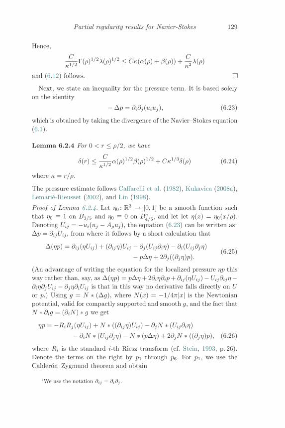
Partial regularity results for Navier-Stokes 129
Hence,
C
κ1/2Γ(ρ)1/2λ(ρ)1/2 ≤ Cκ(α(ρ) + β(ρ)) +
C
κ2λ(ρ)
and (6.12) follows.
Next, we state an inequality for the pressure term. It is based solelyon the identity
− Δp = ∂i∂j(uiuj), (6.23)
which is obtained by taking the divergence of the Navier–Stokes equation(6.1).
Lemma 6.2.4 For 0 < r ≤ ρ/2, we have
δ(r) ≤ C
κ1/2α(ρ)1/2β(ρ)1/2 + Cκ1/3δ(ρ) (6.24)
where κ = r/ρ.
The pressure estimate follows Caffarelli et al. (1982), Kukavica (2008a),Lemarie-Rieusset (2002), and Lin (1998).
Proof of Lemma 6.2.4. Let η0 : R3 → [0, 1] be a smooth function suchthat η0 ≡ 1 on B3/5 and η0 ≡ 0 on Bc
4/5, and let let η(x) = η0(x/ρ).Denoting Uij = −ui(uj −Aρuj), the equation (6.23) can be written as1
Δp = ∂ijUij , from where it follows by a short calculation that
Δ(ηp) = ∂ij(ηUij) + (∂ijη)Uij − ∂j(Uij∂iη) − ∂i(Uij∂jη)
− pΔη + 2∂j((∂jη)p).(6.25)
(An advantage of writing the equation for the localized pressure ηp thisway rather than, say, as Δ(ηp) = pΔη+ 2∂iη∂ip+ ∂ij(ηUij)−Uij∂ijη−∂iη∂jUij − ∂jη∂iUij is that in this way no derivative falls directly on U
or p.) Using g = N ∗ (Δg), where N(x) = −1/4π|x| is the Newtonianpotential, valid for compactly supported and smooth g, and the fact thatN ∗ ∂ig = (∂iN) ∗ g we get
ηp = −RiRj(ηUij) +N ∗ ((∂ijη)Uij) − ∂jN ∗ (Uij∂iη)
− ∂iN ∗ (Uij∂jη) −N ∗ (pΔη) + 2∂jN ∗ ((∂jη)p), (6.26)
where Ri is the standard i-th Riesz transform (cf. Stein, 1993, p. 26).Denote the terms on the right by p1 through p6. For p1, we use theCalderon–Zygmund theorem and obtain
1We use the notation ∂ij = ∂i∂j .
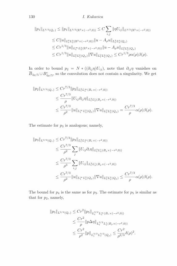
130 I. Kukavica
‖p1‖L3/2(Qr) ≤ ‖p1‖L3/2(R3×(−r2,0)) ≤ C∑i,j
‖ηUij‖L3/2(R3×(−r2,0))
≤ C‖u‖L6t L2
x(R3×(−r2,0))‖u−Aρu‖L2t L6
x(Qρ)
≤ Cr1/3‖u‖L∞t L2
x(R3×(−r2,0))‖u−Aρu‖L2t L6
x(Qρ)
≤ Cr1/3‖u‖L6t L2
x(Qρ)‖∇u‖L2t L2
x(Qρ) ≤ Cr1/3ρα(ρ)β(ρ).
In order to bound p2 = N ∗ ((∂ijη)Uij), note that ∂ijη vanishes onB3ρ/5 ∪Bc
4ρ/5, so the convolution does not contain a singularity. We get
‖p2‖L3/2(Qr) ≤ Cr7/3‖p2‖L2t L∞
x (Br×(−r2,0))
≤ Cr7/3
ρ‖Uij∂ijη‖L2
t L1x(Bρ×(−r2,0))
≤ Cr7/3
ρ2‖u‖L∞
t L2x(Qρ)‖∇u‖L2
t L2x(Qρ) =
Cr7/3
ρα(ρ)β(ρ).
The estimate for p3 is analogous; namely,
‖p3‖L3/2(Qr) ≤ Cr7/3‖p3‖L2t L∞
x (Br×(−r2,0))
≤ Cr7/3
ρ2
∑j
‖Uij∂iη‖L2t L1
x(Bρ×(−r2,0))
≤ Cr7/3
ρ3
∑i,j
‖Uij‖L2t L1
x(Bρ×(−r2,0))
≤ Cr7/3
ρ2‖u‖L∞
t L2x(Qρ)‖∇u‖L2
t L2x(Qρ) ≤
Cr7/3
ρα(ρ)β(ρ).
The bound for p4 is the same as for p3. The estimate for p5 is similar asthat for p2, namely,
‖p5‖L3/2(Qr) ≤ Cr2‖p5‖L3/2t L∞
x (Br×(−r2,0))
≤ Cr2
ρ‖pΔη‖
L3/2t L1
x(Bρ×(−r2,0))
≤ Cr2
ρ2‖p‖
L3/2t L
3/2x (Qρ)
≤ Cr2
ρ2/3δ(ρ)2.
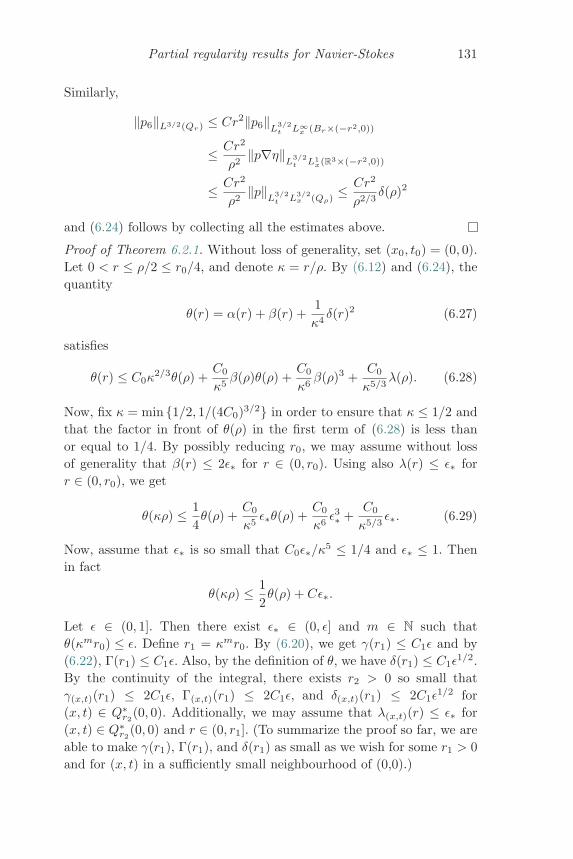
Partial regularity results for Navier-Stokes 131
Similarly,
‖p6‖L3/2(Qr) ≤ Cr2‖p6‖L3/2t L∞
x (Br×(−r2,0))
≤ Cr2
ρ2‖p∇η‖
L3/2t L1
x(R3×(−r2,0))
≤ Cr2
ρ2‖p‖
L3/2t L
3/2x (Qρ)
≤ Cr2
ρ2/3δ(ρ)2
and (6.24) follows by collecting all the estimates above.
Proof of Theorem 6.2.1. Without loss of generality, set (x0, t0) = (0, 0).Let 0 < r ≤ ρ/2 ≤ r0/4, and denote κ = r/ρ. By (6.12) and (6.24), thequantity
θ(r) = α(r) + β(r) +1κ4δ(r)2 (6.27)
satisfies
θ(r) ≤ C0κ2/3θ(ρ) +
C0
κ5β(ρ)θ(ρ) +
C0
κ6β(ρ)3 +
C0
κ5/3λ(ρ). (6.28)
Now, fix κ = min {1/2, 1/(4C0)3/2} in order to ensure that κ ≤ 1/2 andthat the factor in front of θ(ρ) in the first term of (6.28) is less thanor equal to 1/4. By possibly reducing r0, we may assume without lossof generality that β(r) ≤ 2ε∗ for r ∈ (0, r0). Using also λ(r) ≤ ε∗ forr ∈ (0, r0), we get
θ(κρ) ≤ 14θ(ρ) +
C0
κ5ε∗θ(ρ) +
C0
κ6ε3∗ +
C0
κ5/3ε∗. (6.29)
Now, assume that ε∗ is so small that C0ε∗/κ5 ≤ 1/4 and ε∗ ≤ 1. Thenin fact
θ(κρ) ≤ 12θ(ρ) + Cε∗.
Let ε ∈ (0, 1]. Then there exist ε∗ ∈ (0, ε] and m ∈ N such thatθ(κmr0) ≤ ε. Define r1 = κmr0. By (6.20), we get γ(r1) ≤ C1ε and by(6.22), Γ(r1) ≤ C1ε. Also, by the definition of θ, we have δ(r1) ≤ C1ε
1/2.By the continuity of the integral, there exists r2 > 0 so small thatγ(x,t)(r1) ≤ 2C1ε, Γ(x,t)(r1) ≤ 2C1ε, and δ(x,t)(r1) ≤ 2C1ε
1/2 for(x, t) ∈ Q∗
r2(0, 0). Additionally, we may assume that λ(x,t)(r) ≤ ε∗ for
(x, t) ∈ Q∗r2
(0, 0) and r ∈ (0, r1]. (To summarize the proof so far, we areable to make γ(r1), Γ(r1), and δ(r1) as small as we wish for some r1 > 0and for (x, t) in a sufficiently small neighbourhood of (0,0).)

132 I. Kukavica
Fix (x, t) ∈ Q∗r2
(0, 0). By (6.13), max {α(x,t)(κr1), β(x,t)(κr1)} ≤ Cε.Similarly, using the monotonicity of the integral (or by (6.24)), we obtainδ(x,t)(κr1) ≤ Cε1/2. Therefore, θ(x,t)(κr1) ≤ C2ε, where θ(x,t) denotes theanalog of (6.27) centred at (x, t) instead of (0, 0). Now, by (6.28) and bythe definition of κ, we have
θ(x,t)(κρ) ≤ 14θ(x,t)(ρ) + C3θ(x,t)(ρ)3 + C3ε∗.
If ε is so small that C3(C2ε)2 ≤ 1/4 and ε∗ > 0 is so small thatC3ε∗ ≤ C2ε/4, we get θ(x,t)(κnr1) ≤ C2ε for every n ∈ N as long as(x, t) ∈ Q∗
r2(0, 0). By the monotonicity of the integral, it then follows
that θ(x,t)(r) ≤ Cε for all r ∈ (0, r1]. This implies that
α(x,t)(r) + β(x,t)(r) + δ(x,t)(r)2 ≤ Cε
for all r ∈ (0, r1]. By (6.20) and (6.22), we get
max {γ(x,t)(r),Γ(x,t)(r)} ≤ Cε
for all r ∈ (0, r1]. Since (x, t) ∈ Q∗r2
(0, 0) was arbitrary, we conclude that(x0, t0) ∈ R as claimed.
Remark 6.2.5 Theorem 6.2.1 in this section remains valid if (i) isreplaced by(i)′ u ∈ L∞
t L2x(D) ∩ L2
tH1x(D) and p ∈ Lq
tL1x(D), where q > 1,
and the inequality (6.3) in the definition of a regular point is replacedby
1r2/3
‖u‖L3(Qr) +1
r2/q−1/2‖p‖Lq
t L2x(Qr) ≤ μ.
Observe that, by elliptic regularity, we get
p ∈⋂
1<s≤3
L2s/(3s−3)t Ls
x(Qρ) + LqtL
∞x (Qρ).
The proof is similar to the proof of Theorem 6.2.1. The inequality (6.12)is replaced by
α(r) + β(r) ≤ Cκ2/3(α(ρ) + β(ρ)
)+C
κ6β(ρ)3 +
C
κα(ρ)β(ρ)1/2
+1
κ8/3Δ(ρ)2 +
C
κ5/3λ(ρ),
where
Δ(r) =1
r1/q−1/4‖p‖1/2
Lqt L2
x(Qr).
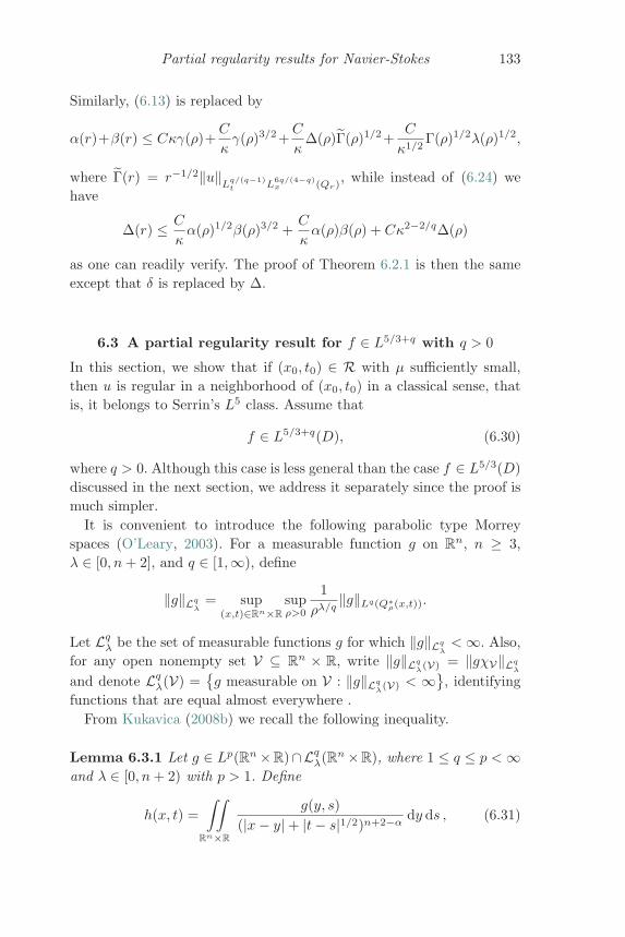
Partial regularity results for Navier-Stokes 133
Similarly, (6.13) is replaced by
α(r)+β(r) ≤ Cκγ(ρ)+C
κγ(ρ)3/2+
C
κΔ(ρ)Γ(ρ)1/2+
C
κ1/2Γ(ρ)1/2λ(ρ)1/2,
where Γ(r) = r−1/2‖u‖L
q/(q−1)t L
6q/(4−q)x (Qr)
, while instead of (6.24) wehave
Δ(r) ≤ C
κα(ρ)1/2β(ρ)3/2 +
C
κα(ρ)β(ρ) + Cκ2−2/qΔ(ρ)
as one can readily verify. The proof of Theorem 6.2.1 is then the sameexcept that δ is replaced by Δ.
6.3 A partial regularity result for f ∈ L5/3+q with q > 0
In this section, we show that if (x0, t0) ∈ R with μ sufficiently small,then u is regular in a neighborhood of (x0, t0) in a classical sense, thatis, it belongs to Serrin’s L5 class. Assume that
f ∈ L5/3+q(D), (6.30)
where q > 0. Although this case is less general than the case f ∈ L5/3(D)discussed in the next section, we address it separately since the proof ismuch simpler.
It is convenient to introduce the following parabolic type Morreyspaces (O’Leary, 2003). For a measurable function g on Rn, n ≥ 3,λ ∈ [0, n+ 2], and q ∈ [1,∞), define
‖g‖Lqλ
= sup(x,t)∈Rn×R
supρ>0
1ρλ/q
‖g‖Lq(Q∗ρ(x,t)).
Let Lqλ be the set of measurable functions g for which ‖g‖Lq
λ<∞. Also,
for any open nonempty set V ⊆ Rn × R, write ‖g‖Lqλ(V) = ‖gχV‖Lq
λ
and denote Lqλ(V) =
{g measurable on V : ‖g‖Lq
λ(V) < ∞}, identifying
functions that are equal almost everywhere .From Kukavica (2008b) we recall the following inequality.
Lemma 6.3.1 Let g ∈ Lp(Rn ×R)∩Lqλ(Rn ×R), where 1 ≤ q ≤ p <∞
and λ ∈ [0, n+ 2) with p > 1. Define
h(x, t) =∫∫
Rn×R
g(y, s)(|x− y| + |t− s|1/2)n+2−α
dy ds , (6.31)
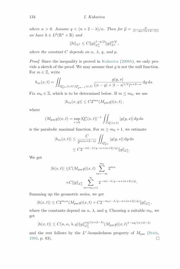
134 I. Kukavica
where α > 0. Assume q < (n+ 2 − λ)/α. Then for p = p(1−qα/(n+2−λ))
we have h ∈ Lp(Rn × R) and
‖h‖Lp ≤ C‖g‖1−p/p
Lqλ
‖g‖p/pLp ,
where the constant C depends on α, λ, q, and p.
Proof. Since the inequality is proved in Kukavica (2008b), we only pro-vide a sketch of the proof. We may assume that g is not the null function.For m ∈ Z, write
hm(x, t) =∫∫
Q∗2m (x,t)\Q∗
2m−1 (x,t)
g(y, s)(|x− y| + |t− s|1/2)n+2−α
dy ds.
Fix m0 ∈ Z, which is to be determined below. If m ≤ m0, we use
|hm(x, y)| ≤ C2mα(Mparg)(x, t) ,
where
(Mparg)(x, t) = supr>0
|Q∗r(x, t)|−1
∫∫Q∗
r(x,t)
|g(y, s)|dy ds
is the parabolic maximal function. For m ≥ m0 + 1, we estimate
|hm(x, t)| ≤ C
2m(n+2−α)
∫∫Q∗
2m
|g(y, s)|dy ds
≤ C2−m(−λ/q−α+(n+2)/q)‖g‖Lqλ.
We get
|h(x, t)| ≤C(Mparg)(x, t)m0∑
m=−∞2mα
+C‖g‖Lqλ
∞∑m=m0+1
2−m(−λ/q−α+(n+2)/q).
Summing up the geometric series, we get
|h(x, t)| ≤ C2m0α(Mparg)(x, t) + C2−m0(−λ/q−α+(n+2)/q)‖g‖Lqλ,
where the constants depend on α, λ, and q. Choosing a suitable m0, weget
|h(x, t)| ≤ C(n, α, λ, q)‖g‖αq/(n+2−λ)
Lqλ
(Mparg)(x, t)1−αq/(n+2−λ)
and the rest follows by the Lr-boundedness property of Mpar (Stein,1993, p. 83).
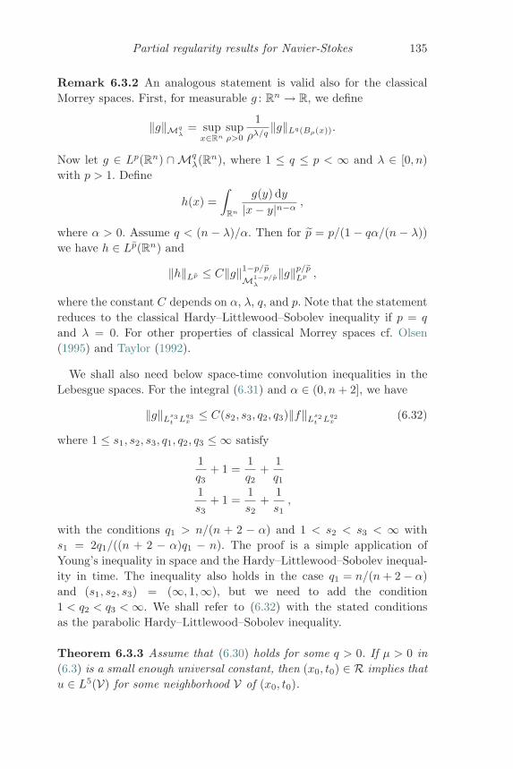
Partial regularity results for Navier-Stokes 135
Remark 6.3.2 An analogous statement is valid also for the classicalMorrey spaces. First, for measurable g : Rn → R, we define
‖g‖Mqλ
= supx∈Rn
supρ>0
1ρλ/q
‖g‖Lq(Bρ(x)).
Now let g ∈ Lp(Rn) ∩ Mqλ(Rn), where 1 ≤ q ≤ p < ∞ and λ ∈ [0, n)
with p > 1. Define
h(x) =∫
Rn
g(y) dy|x− y|n−α
,
where α > 0. Assume q < (n − λ)/α. Then for p = p/(1 − qα/(n − λ))we have h ∈ Lp(Rn) and
‖h‖Lp ≤ C‖g‖1−p/p
M1−p/pλ
‖g‖p/pLp ,
where the constant C depends on α, λ, q, and p. Note that the statementreduces to the classical Hardy–Littlewood–Sobolev inequality if p = q
and λ = 0. For other properties of classical Morrey spaces cf. Olsen(1995) and Taylor (1992).
We shall also need below space-time convolution inequalities in theLebesgue spaces. For the integral (6.31) and α ∈ (0, n+ 2], we have
‖g‖Ls3t L
q3x
≤ C(s2, s3, q2, q3)‖f‖Ls2t L
q2x
(6.32)
where 1 ≤ s1, s2, s3, q1, q2, q3 ≤ ∞ satisfy
1q3
+ 1 =1q2
+1q1
1s3
+ 1 =1s2
+1s1,
with the conditions q1 > n/(n + 2 − α) and 1 < s2 < s3 < ∞ withs1 = 2q1/((n + 2 − α)q1 − n). The proof is a simple application ofYoung’s inequality in space and the Hardy–Littlewood–Sobolev inequal-ity in time. The inequality also holds in the case q1 = n/(n+ 2 − α)and (s1, s2, s3) = (∞, 1,∞), but we need to add the condition1 < q2 < q3 <∞. We shall refer to (6.32) with the stated conditionsas the parabolic Hardy–Littlewood–Sobolev inequality.
Theorem 6.3.3 Assume that (6.30) holds for some q > 0. If μ > 0 in(6.3) is a small enough universal constant, then (x0, t0) ∈ R implies thatu ∈ L5(V) for some neighborhood V of (x0, t0).
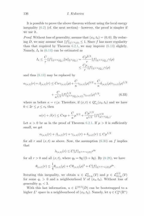
136 I. Kukavica
It is possible to prove the above theorem without using the local energyinequality (6.2) (cf. the next section)—however, the proof is simpler ifwe use it.
Proof. Without loss of generality, assume that (x0, t0) = (0, 0). By reduc-ing D, we may assume that ‖f‖L5/3(D) ≤ 1. Since f has more regularitythan that required by Theorem 6.2.1, we may improve (6.13) slightly.Namely, I4 in (6.14) can be estimated as
I4 ≤ C
r‖f‖L3/2(Qρ)‖u‖L3(Qρ) =
Cρ2/3
r‖f‖L3/2(Qρ)γ(ρ)
≤ Cρ
r‖f‖L5/3(Qρ)γ(ρ)
and thus (6.13) may be replaced by
α(x,t)(r)+β(x,t)(r) ≤ Cκγ(x,t)(ρ)+C
κγ(x,t)(ρ)3/2 +
C
κδ(x,t)(ρ)γ(x,t)(ρ)1/2
+C
κ1/2‖f‖1/2
L5/3(Qρ(x,t))γ(x,t)(ρ)1/2, (6.33)
where as before κ = r/ρ. Therefore, if (x, t) ∈ Q∗r0
(x0, t0) and we have0 < 2r ≤ ρ ≤ r0 then
α(r) + β(r) ≤ Cκμ+C
κμ3/2 +
Cμ1/2
κ1/2‖f‖1/2
L5/3(Qρ).
Let κ > 0 be as in the proof of Theorem 6.2.1. If μ > 0 is sufficientlysmall, we get
α(x,t)(r) + β(x,t)(r) + γ(x,t)(r) + δ(x,t)(r) ≤ Cμ1/2
for all r and (x, t) as above. Now, the assumption (6.30) on f impliesthat
λ(x,t)(r) ≤ C‖f‖L5/3+q(D)rq0
for all r > 0 and all (x, t), where q0 = 9q/(5 + 3q). By (6.28), we have
θ(x,t)(r) ≤ 14θ(x,t)(ρ) + Cθ(x,t)(ρ)3 + C‖f‖L5/3+q(D)ρ
q0 .
Iterating this inequality, we obtain u ∈ L32+q1
(V) and p ∈ L3/22+q1
(V)for some q1 > 0 and a neighbourhood V of (x0, t0). Without loss ofgenerality q1 < 3.
With this last information, u ∈ L10/3(D) can be bootstrapped to ahigher Lr space in a neighbourhood of (x0, t0). Namely, let η ∈ C∞
0 (Rn)
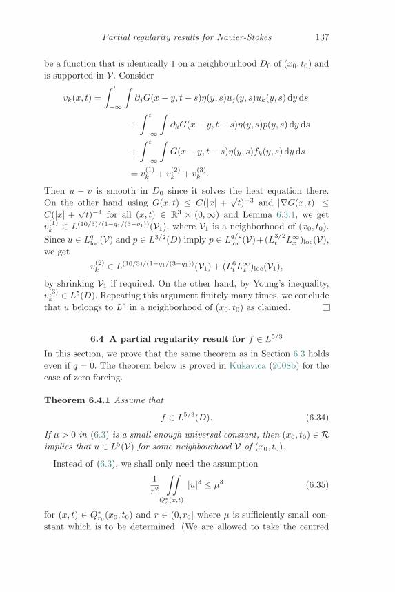
Partial regularity results for Navier-Stokes 137
be a function that is identically 1 on a neighbourhood D0 of (x0, t0) andis supported in V. Consider
vk(x, t) =∫ t
−∞
∫∂jG(x− y, t− s)η(y, s)uj(y, s)uk(y, s) dy ds
+∫ t
−∞
∫∂kG(x− y, t− s)η(y, s)p(y, s) dy ds
+∫ t
−∞
∫G(x− y, t− s)η(y, s)fk(y, s) dy ds
= v(1)k + v
(2)k + v
(3)k .
Then u − v is smooth in D0 since it solves the heat equation there.On the other hand using G(x, t) ≤ C(|x| +
√t)−3 and |∇G(x, t)| ≤
C(|x| +√t)−4 for all (x, t) ∈ R3 × (0,∞) and Lemma 6.3.1, we get
v(1)k ∈ L(10/3)/(1−q1/(3−q1))(V1), where V1 is a neighborhood of (x0, t0).
Since u ∈ Lqloc(V) and p ∈ L3/2(D) imply p ∈ L
q/2loc (V)+(L3/2
t L∞x )loc(V),
we get
v(2)k ∈ L(10/3)/(1−q1/(3−q1))(V1) + (L6
tL∞x )loc(V1),
by shrinking V1 if required. On the other hand, by Young’s inequality,v(3)k ∈ L5(D). Repeating this argument finitely many times, we conclude
that u belongs to L5 in a neighborhood of (x0, t0) as claimed.
6.4 A partial regularity result for f ∈ L5/3
In this section, we prove that the same theorem as in Section 6.3 holdseven if q = 0. The theorem below is proved in Kukavica (2008b) for thecase of zero forcing.
Theorem 6.4.1 Assume that
f ∈ L5/3(D). (6.34)
If μ > 0 in (6.3) is a small enough universal constant, then (x0, t0) ∈ Rimplies that u ∈ L5(V) for some neighbourhood V of (x0, t0).
Instead of (6.3), we shall only need the assumption
1r2
∫∫Q∗
r(x,t)
|u|3 ≤ μ3 (6.35)
for (x, t) ∈ Q∗r0
(x0, t0) and r ∈ (0, r0] where μ is sufficiently small con-stant which is to be determined. (We are allowed to take the centred
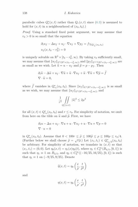
138 I. Kukavica
parabolic cubes Q∗r(x, t) rather than Qr(x, t) since (6.3) is assumed to
hold for (x, t) in a neighbourhood of (x0, t0).)
Proof. Using a standard fixed point argument, we may assume thatr0 > 0 is so small that the equation
∂tuf − Δuf + uf · ∇uf + ∇pf = fχQ∗r0
(x0,t0)
uf (x, t0 − r20) = 0
is uniquely solvable on R3 × [t0 − r20,∞). By taking r0 sufficiently small,we may assume that ‖uf‖L5(R3×(t0−r2
0 ,∞)) and ‖pf‖L5/2(R3×(t0−r20 ,∞)) are
as small as we wish. Let u = u− uf and p = p− pf . Then
∂tu− Δu+ uf · ∇u+ u · ∇uf + u · ∇u+ ∇p = f
∇ · u = 0,
where f vanishes in Q∗r0
(x0, t0). Since ‖uf‖L5(R3×(t0−r20 ,∞)) is as small
as we wish, we may assume that ‖uf‖L5(R3×(t0−r20,∞)) and
1r2
∫∫Q∗
r(x,t)
|u|3 ≤ 2μ3
for all (x, t) ∈ Q∗r0
(x0, t0) and r ≤ r0. For simplicity of notation, we omitfrom here on the tilde on u and p. First, we have
∂tu− Δu+ uf · ∇u+ u · ∇uf + u · ∇u+ ∇p = 0
∇ · u = 0
in Q∗r0
(x0, t0). Assume that 0 < 100r ≤ ρ ≤ 100ρ ≤ ρ ≤ 100ρ ≤ r0/4.(Further below we shall choose ρ =
√rρ.) Let (x1, t1) ∈ Q∗
r0/2(x0, t0)be arbitrary. For simplicity of notation, we translate in (x, t) so that(x1, t1) = (0, 0). Let η0(x, t) = η1(x)η2(t), where η1 ∈ C∞
0 (B4/5, [0, 1]) issuch that η1 ≡ 1 on B3/5, and η2 ∈ C∞
0 ((−16/25, 16/25), [0, 1]) is suchthat η1 ≡ 1 on (−9/25, 9/25). Denote
η(x, t) = η0
(x
ρ,t
ρ2
)and
η(x, t) = η0
(x
ρ,t
ρ2
)
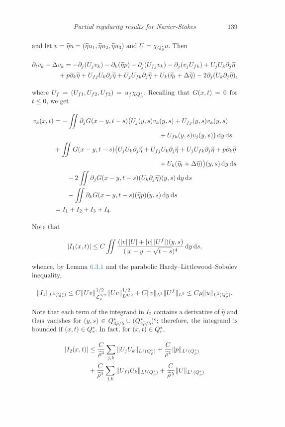
Partial regularity results for Navier-Stokes 139
and let v = ηu = (ηu1, ηu2, ηu3) and U = χQ∗ρu. Then
∂tvk − Δvk = −∂j(Ujvk) − ∂k(ηp) − ∂j(Ufjvk) − ∂j(vjUfk) + UjUk∂j η
+ p∂kη + UfjUk∂j η + UjUfk∂j η + Uk(ηt + Δη) − 2∂j(Uk∂j η),
where Uf = (Uf1, Uf2, Uf3) = ufχQ∗ρ. Recalling that G(x, t) = 0 for
t ≤ 0, we get
vk(x, t) = −∫∫
∂jG(x− y, t− s)(Uj(y, s)vk(y, s) + Ufj(y, s)vk(y, s)
+ Ufk(y, s)vj(y, s))
dy ds
+∫∫
G(x− y, t− s)(UjUk∂j η + UfjUk∂j η + UjUfk∂j η + p∂kη
+ Uk(ηt + Δη))(y, s) dy ds
− 2∫∫
∂jG(x− y, t− s)(Uk∂j η)(y, s) dy ds
−∫∫
∂kG(x− y, t− s)(ηp)(y, s) dy ds
= I1 + I2 + I3 + I4.
Note that
|I1(x, t)| ≤ C
∫∫(|v| |U | + |v| |Uf |)(y, s)
(|x− y| +√t− s)4
dy ds,
whence, by Lemma 6.3.1 and the parabolic Hardy–Littlewood–Sobolevinequality,
‖I1‖L3(Q∗r) ≤ C‖Uv‖1/2
L3/22
‖Uv‖1/2
L3/2 + C‖v‖L3‖Uf‖L5 ≤ Cμ‖u‖L3(Q∗ρ).
Note that each term of the integrand in I2 contains a derivative of η andthus vanishes for (y, s) ∈ Q∗
3ρ/5 ∪ (Q∗4ρ/5)c; therefore, the integrand is
bounded if (x, t) ∈ Q∗r . In fact, for (x, t) ∈ Q∗
r ,
|I2(x, t)| ≤ C
ρ4
∑j,k
‖UjUk‖L1(Q∗ρ) +
C
ρ4‖p‖L1(Q∗
ρ)
+C
ρ4
∑j,k
‖UfjUk‖L1(Q∗ρ) +
C
ρ 5‖U‖L1(Q∗
ρ)
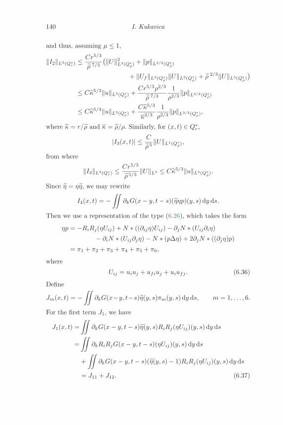
140 I. Kukavica
and thus, assuming μ ≤ 1,
‖I2‖L3(Q∗r) ≤ Cr5/3
ρ 7/3
(‖U‖2L3(Q∗
ρ) + ‖p‖L3/2(Q∗
ρ)
+ ‖Uf‖L3(Q∗ρ)‖U‖L3(Q∗
ρ) + ρ 2/3‖U‖L3(Q∗
ρ)
)≤ Cκ5/3‖u‖L3(Q∗
ρ) +
Cr5/3ρ2/3
ρ 7/3
1ρ2/3
‖p‖L3/2(Q∗ρ)
≤ Cκ5/3‖u‖L3(Q∗ρ) +
Cκ5/3
κ2/3
1ρ2/3
‖p‖L3/2(Q∗ρ),
where κ = r/ρ and κ = ρ/ρ. Similarly, for (x, t) ∈ Q∗r ,
|I3(x, t)| ≤ C
ρ 5‖U‖L1(Q∗
ρ),
from where
‖I3‖L3(Q∗r) ≤ Cr5/3
ρ 5/3‖U‖L3 ≤ Cκ5/3‖u‖L3(Q∗
ρ).
Since η = ηη, we may rewrite
I4(x, t) = −∫∫
∂kG(x− y, t− s)(ηηp)(y, s) dy ds.
Then we use a representation of the type (6.26), which takes the form
ηp = −RiRj(ηUij) +N ∗ ((∂ijη)Uij) − ∂jN ∗ (Uij∂iη)
− ∂iN ∗ (Uij∂jη) −N ∗ (pΔη) + 2∂jN ∗ ((∂jη)p)
= π1 + π2 + π3 + π4 + π5 + π6,
where
Uij = uiuj + ufiuj + uiufj . (6.36)
Define
Jm(x, t) = −∫∫
∂kG(x−y, t−s)η(y, s)πm(y, s) dy ds, m = 1, . . . , 6.
For the first term J1, we have
J1(x, t) =∫∫
∂kG(x− y, t− s)η(y, s)RiRj(ηUij)(y, s) dy ds
=∫∫
∂kRiRjG(x− y, t− s)(ηUij)(y, s) dy ds
+∫∫
∂kG(x− y, t− s)(η(y, s) − 1)RiRj(ηUij)(y, s) dy ds
= J11 + J12. (6.37)
Partial regularity results for Navier-Stokes 141
For the term J11, we have by Fabes et al. (1972),
|∇RiRjG(x, t)| ≤ C
(|x| +√t)4
, x ∈ R3, t > 0, i, j = 1, 2, 3.
Using Lemma 6.3.1 and the parabolic Hardy–Littlewood–Sobolevinequality, we obtain
‖J11‖L3(Q∗r) ≤ C‖ηuiuj‖1/2
L3/22
‖ηuiuj‖1/2
L3/2 + C∑i,j
‖ηuiufj‖L15/8
≤ Cμ‖u‖L3(Q∗ρ).
For the term J12, note that η − 1 vanishes on Q∗ρ/2. Therefore,
|J12(x, t)| ≤ C
∫∫Q∗
ρ/2(x,t)c
|RiRj(ηuiuj)(y, s)| + |RiRj(ηufiuj)(y, s)|(|x− y| + |t− s|1/2)4
dy ds
for (x, t) ∈ Q∗r . Then write
Q∗ρ/2(x, t)c =
∞⋃m=0
(Q∗
2mρ(x, t) ∩Q∗2m−1ρ(x, t)c
)and obtain
|J12(x, t)| ≤∞∑
m=0
C
24mρ4
(‖RiRj(ηuiuj)‖L1(Q∗
2mρ(x,t)∩Q∗
2m−1ρ(x,t)c)
+ ‖RiRj(ηufiuj)‖L1(Q∗2mρ
(x,t)∩Q∗2m−1ρ
(x,t)c)
)≤
∞∑m=0
C
27m/3ρ 7/3
(‖RiRj(ηuiuj)‖L3/2(Q∗
2mρ(x,t)∩Q∗
2m−1ρ(x,t)c)
+ ‖RiRj(ηufiuj)‖L3/2(Q∗2mρ
(x,t)∩Q∗2m−1ρ
(x,t)c)
)≤
∞∑m=0
C
27m/3ρ 7/3
(∑i,j
‖ηuiuj‖L3/2(R3×(−ρ2,ρ2))
+∑i,j
‖ηufiuj‖L3/2(R3×(−ρ2,ρ2))
)
≤∞∑
m=0
C
27m/3ρ 7/3
(‖u‖2
L3(Q∗ρ) + ‖u‖L3(Q∗
ρ)‖uf‖L3(Q∗ρ)
)≤ Cμρ2/3
ρ 7/3‖u‖L3(Q∗
ρ)
142 I. Kukavica
for (x, t) ∈ Q∗r . Therefore,
‖J12‖L3(Q∗r) ≤ Cr5/3‖J12‖L∞(Q∗
r) ≤ Cμκ5/3
κ2/3‖u‖L3(Q∗
r).
Next, using the parabolic Hardy–Littlewood–Sobolev inequality, we get
‖J2‖L3(Q∗r) ≤ Cr7/10‖J2‖L3
t L10x (Q∗
r) ≤ Cr7/10‖ηπ2‖L3/2t L
90/19x
≤ Cr7/10ρ19/30‖N ∗ ((∂ijη)Uij)‖L
3/2t L∞
x (Q∗ρ).
Now, note that, by the construction of η, we have ∂ijη(y, s) = 0 on theset {(y, s) : |y| ≤ 3/5}. Therefore, the convolution above is not singular,and we have ‖N ∗ ((∂ijη)Uij)‖
L3/2t L∞
x (Q∗ρ)≤ Cρ−3‖U‖
L3/2t L1
x(Q∗ρ)
, and
thus
‖J2‖L3(Q∗r) ≤ Cr7/10ρ 19/30
ρ3‖U‖
L3/2t L1
x(Q∗ρ)
≤ Cr7/10ρ 19/30
ρ2‖U‖L3/2(Q∗
ρ)
≤ Cμr7/10ρ 19/30
ρ4/3‖u‖L3(Q∗
ρ) ≤ Cμ‖u‖L3(Q∗ρ).
The same upper bounds can be derived for J3 and J4. As for J5, we haveby the parabolic Hardy–Littlewood–Sobolev inequality
‖J5‖L3(Q∗r) ≤ Cr7/10‖J5‖L3
t L10x (Q∗
r) ≤ Cr7/10‖ηπ5‖L3/2t L
90/19x
≤ Cr7/10ρ 19/30‖N ∗ (pΔη)‖L
3/2t L∞
x (Q∗ρ)
≤ Cr7/10ρ 19/30
ρ3‖p‖
L3/2t L1
x(Q∗ρ)
≤ Cr7/10ρ 19/30
ρ2‖p‖L3/2(Q∗
ρ) = Cκ7/10κ4/3 1ρ2/3
‖p‖L3/2(Q∗ρ).
The same estimate holds also for J6. In summary, we get
‖u‖L3(Q∗r) ≤ C
(μ+ κ5/3 +
μκ5/3
κ2/3
)‖u‖L3(Q∗
ρ)
+ C
(κ5/3
κ2/3+ κ7/10κ4/3
)1ρ2/3
‖p‖L3/2(Q∗ρ).
Setting ρ =√ρr, we have κ = κ = κ1/2, where κ = r/ρ, and thus the
inequality reduces to
‖u‖L3(Q∗r) ≤ C(μ+ κ5/6)‖u‖L3(Q∗
ρ) +Cκ1/2
ρ2/3‖p‖L3/2(Q∗
ρ)
Partial regularity results for Navier-Stokes 143
whence
1r2/3
‖u‖L3(Q∗r) ≤ C
( μ
κ2/3+ κ1/6
) 1ρ2/3
‖u‖L3(Q∗ρ) +
C
κ1/6ρ4/3‖p‖L3/2(Q∗
ρ).
By a similar estimate for the pressure, we get
‖p‖L3/2(Q∗r) ≤ C‖u‖2
L3(Q∗ρ) + C‖u‖L3(Q∗
ρ)‖uf‖L3(Q∗ρ) + Cκ2‖p‖L3(Q∗
ρ)
≤ Cμρ2/3‖u‖L3(Q∗ρ) + Cκ2‖p‖L3(Q∗
ρ),
from where
1r4/3
‖p‖L3/2(Q∗ρ) ≤
Cμ
κ4/3ρ2/3‖u‖L3(Q∗
ρ) +Cκ2/3
ρ4/3‖p‖L3/2(Q∗
ρ). (6.38)
The function θ(r) = r−2/3‖u‖L3(Q∗r) + κ−1/3r−4/3‖p‖L3/2(Q∗
r) satisfies
θ(r) ≤ C( μ
κ5/3+ κ1/6
)θ(ρ). (6.39)
Next, choosing κ and μ as appropriate constants (first we choose κ
sufficiently small and then μ sufficiently small compared to κ5/3), theequation (6.39) becomes
θ(κρ) ≤ 12θ(ρ) (6.40)
provided that 0 < ρ < r0/C with C a sufficiently large universalconstant. Iterating this inequality, we get existence of ε > 0 such that
1r2+ε
∫∫Q∗
r(x1,t1)
(|u|3 + |p|3/2) ≤ μ3 (6.41)
for all (x1, t1) is a neighbourhood of (x0, t0) and all sufficiently smallr > 0. Now, this condition is no longer critical, so we may bootstrap as inthe previous section and obtain u ∈ L5(D0), where D0 is a neighborhoodof (x0, t0).
Acknowledgements
I would like to thank James Robinson, Jose Rodrigo, and Vlad Vicol foruseful remarks and suggestions. The work was supported in part by theNSF grant DMS-0604886.
144 I. Kukavica
References
Caffarelli, L., Kohn, R. & Nirenberg, L. (1982) Partial regularity of suitableweak solutions of the Navier–Stokes equations. Comm. Pure Appl. Math.35, no. 6, 771–831.
Constantin, P. & Foias, C. (1988) Navier–Stokes equations. Chicago Lecturesin Mathematics, University of Chicago Press, Chicago, IL.
Fabes, E.B., Jones, B.F. & Riviere, N.M. (1972) The initial value problemfor the Navier–Stokes equations with data in Lp. Arch. Rational Mech.Anal. 45, 222–240.
Hopf, E. (1951) Uber die Anfangswertaufgabe fur die hydrodynamischenGrundgleichungen. Math. Nachr. 4, 213–231.
Kukavica, I. (2008a) On partial regularity for the Navier–Stokes equations.Discrete Contin. Dynam. Systems 21, no. 3, 717–728.
Kukavica, I. (2008b) Regularity for the Navier–Stokes equations with asolution in a Morrey space. Indiana Univ. Math. J. 57, no. 6, 2843–2860.
Ladyzhenskaya O.A. & Seregin, G.A. (1999) On partial regularity of suit-able weak solutions to the three-dimensional Navier–Stokes equations. J.Math. Fluid Mech. 1, no. 4, 356–387.
Lemarie-Rieusset, P.G. (2002) Recent developments in the Navier–Stokesproblem. Chapman & Hall/CRC Research Notes in Mathematics, 431,Chapman & Hall/CRC, Boca Raton, FL.
Leray, J. (1934) Sur le mouvement d’un liquide visqueux emplissant l’espace.Acta Math. 63, no. 1, 193–248.
Lin, F. (1998) A new proof of the Caffarelli–Kohn–Nirenberg theorem. Comm.Pure Appl. Math. 51, no. 3, 241–257.
O’Leary, M. (2003) Conditions for the local boundedness of solutions of theNavier–Stokes system in three dimensions. Comm. Partial DifferentialEquations 28, no. 3-4, 617–636.
Olsen, P.A. (1995) Fractional integration, Morrey spaces and a Schrodingerequation. Comm. Partial Differential Equations 20, no. 11–12,2005–2055.
Robinson J.C. & Sadowski, W. (2007) Decay of weak solutions and the singularset of the three-dimensional Navier–Stokes equations. Nonlinearity 20,no. 5, 1185–1191.
Scheffer, V. (1976a) Partial regularity of solutions to the Navier–Stokesequations. Pacific J. Math. 66, no. 2, 535–552.
Scheffer, V. (1976b) Turbulence and Hausdorff dimension. Turbulence andNavier–Stokes equations (Proc. Conf., Univ. Paris-Sud, Orsay, 1975).Lecture Notes in Math. 565, 174–183. Springer, Berlin.
Scheffer, V. (1977) Hausdorff measure and the Navier–Stokes equations.Comm. Math. Phys. 55, no. 2, 97–112.
Serrin, J. (1962) On the interior regularity of weak solutions of the Navier–Stokes equations. Arch. Rational Mech. Anal. 9, 187–195.
Serrin, J. (1963) The initial value problem for the Navier–Stokes equations.Nonlinear Problems (Proc. Sympos., Madison, Wis.) 69–98. Univ. ofWisconsin Press, Madison, Wis.
Sohr, H. (1983) Zur Regularitatstheorie der instationaren Gleichungen vonNavier–Stokes. Math. Z. 184, no. 3, 359-375.
Struwe, M. (1998) On partial regularity results for the Navier–Stokes equa-tions. Comm. Pure Appl. Math. 41, no. 4, 437–458.
Partial regularity results for Navier-Stokes 145
Stein, E.M. (1993) Harmonic analysis: real-variable methods, orthogonality,and oscillatory integrals. Princeton Mathematical Series, 43, PrincetonUniversity Press, Princeton, NJ.
Taylor, M.E. (1992) Analysis on Morrey spaces and applications to Navier–Stokes and other evolution equations Comm. Partial Differential Equa-tions 17 (1992), no. 9-10, 1407–1456.
Temam, R. (2001) Navier–Stokes equations: Theory and numerical analysis.AMS Chelsea Publishing, Providence, RI. Reprint of the 1984 edition.
Vasseur, A.F.(2007) A new proof of partial regularity of solutions to Navier-Stokes equations. NoDEA Nonlinear Differential Equations Appl. 14,no. 5-6, 753–785.
7
Anisotropic Navier–Stokes equations in abounded cylindrical domain
Marius PaicuUniv Paris-Sud and CNRS, Laboratoire de Mathematiques d’Orsay,
Orsay Cedex, F-91405. [email protected]
Genevieve RaugelCNRS and Univ Paris-Sud, Laboratoire de Mathematiques d’Orsay,
Orsay Cedex, F-91405. [email protected]
Abstract
In this paper, we study the global and local existence and uniquenessof solutions to the Navier–Stokes equations with anisotropic viscosity ina bounded cylindrical domain Q = Ω × (0, 1), where Ω is a star-shapeddomain in R2. Here we consider the case of homogeneous Dirichletboundary conditions on the lateral boundary and vanishing normal traceon the top and the bottom of the cylinder.
7.1 Introduction
The Navier–Stokes equations with anisotropic viscosity are classicalin geophysical fluid dynamics. Instead of choosing the more standardviscosity −ν(∂2
1 + ∂22 + ∂2
3) in the case of three-dimensional fluids, mete-orologists often model turbulent flows using a viscosity of the form−νh(∂2
1 + ∂22) − νv∂
23 , where νv is usually much smaller than νh and
thus can be neglected (see Chapter 4 in Pedlosky (1979), for a detaileddiscussion).
More precisely, in geophysical fluids, the rotation of the earth playsa crucial role. The Coriolis force introduces a penalized skew-symmetricterm ε−1u × e3 into the equations, where ε > 0 is the Rossby num-ber and e3 = (0, 0, 1) is the unit vertical vector. This leads to anasymmetry between the horizontal and vertical motions. By the Taylor–Proudman Theorem (see Pedlosky (1979) and Taylor (1923)), the fluidtends to have a two-dimensional behaviour far from the boundary of thedomain. When the fluid evolves between two parallel plates with homo-geneous Dirichlet boundary conditions, Ekman boundary layers of the
Published in Partial Differential Equations and Fluid Mechanics, edited byJames C. Robinson and Jose L. Rodrigo. c© Cambridge University Press 2009.
Anisotropic Navier–Stokes equations in a bounded cylinder 147
form UBL(x1, x2, ε−1x3) appear near the boundary. In order to compen-
sate the term ε−1UBL × e3 by the term −νv∂23UBL, we need to impose
the requirement that νv = βε, for β > 0 (Grenier & Masmoudi, 1997;Chemin et al., 2006).
When the fluid occupies the whole space, the Navier–Stokes equationswith vanishing or small vertical viscosity are as follows:
∂tu+ u∇u− νh(∂21 + ∂2
2)u− νv∂23u = −∇p in R3 , t > 0
div u = 0 in R3 , t > 0
u|t=0 = u0,
(7.1)
where νh > 0 and νv ≥ 0 represent the horizontal and vertical viscositiesand where u = (u1, u2, u3) and p are the vector field of the velocities andthe pressure respectively. In the case of vanishing vertical viscosity, theclassical theory of the Navier–Stokes equations does not apply and newdifficulties arise. Some partial L2-energy estimates still hold for system(7.1), but they do not allow one to pass to the limit and to obtain a weaksolution as in the well-known construction of weak Leray solutions nor touse directly the results of Fujita & Kato (1964) on the existence of strongsolutions. Of course, neglecting the horizontal viscosity and requiring alot of regularity of the initial data, one can prove the local existence ofstrong solutions within the framework of hyperbolic symmetric systems.Thus, new methods have to be developed.
In the case νv = 0, this system was first studied by Chemin et al.(2000), who showed local and global existence of solutions in anisotropicSobolev spaces which take into account this anisotropy. More precisely,for s ≥ 0, let us introduce the anisotropic Sobolev spaces,
H0,s = {u ∈ L2(R3)3 | ‖u‖2H0,s =
∫R3
(1 + |ξ3|2)s|u(ξ)|2 dξ < +∞}
and H1,s = {u ∈ H0,s | ∂iu ∈ H0,s , i = 1, 2} (such anisotropic spaceswere introduced in Iftimie (1999) for the study of the Navier–Stokessystem in thin domains).
Chemin et al. (2000) showed that, for any s0 > 1/2, and any u0 ∈H0,s0 , there exist T > 0 and a local solution
u ∈ L∞((0, T ),H0,s0) ∩ L2((0, T ),H1,s0)
of the anisotropic Navier–Stokes equations (7.1). If ‖u0‖H0,s0 ≤ cνh,where c > 0 is a small constant, then the solution is global in time. Inthe same paper, the authors proved that there exists at most one solutionu(t) of the equations (7.1) in the space L∞((0, T ),H0,s)∩L2((0, T ),H1,s)
148 M. Paicu & G. Raugel
for s > 3/2. In these results, there was a gap between the regularityrequired for the existence of solutions and that required for uniqueness.This gap was closed by Iftimie (2002) who showed the uniqueness of thesolution in the space L∞((0, T ),H0,s) ∩ L2((0, T ),H1,s) for s > 1/2.
Like the classical Navier–Stokes equations, the system (7.1) on thewhole space R3 has a scaling. Indeed, if u is a solution of the equa-tions (7.1) on a time interval [0, T ] with initial data u0, then uμ(t, x) =μu(μ2t, μx) is also a solution of (7.1) on the time interval [0, μ−2T ], withinitial data μu0(μx). This was one of the motivations of Paicu for con-sidering initial data in the scaling invariant Besov space B0,1/2. Paicu(2005b) proved the local existence and uniqueness of the solutions of(7.1), for initial data u0 ∈ B0,1/2. He showed global existence of thesolution when the initial data in B0,1/2 are small, compared to the hor-izontal viscosity νh (for further details see Paicu, 2004, 2005a,b). Veryrecently Chemin & Zhang (2007) introduced the scaling invariant Besov–Sobolev spaces B−1/2,1/2
4 and showed existence of global solutions whenthe initial data u0 in B−1/2,1/2
4 are small compared to the horizontalviscosity νh. This result implies the global well-posedness of (7.1) withhighly oscillatory initial data.
Notice that in all the above results, as well as in this paper, one ofthe key observations is that, in the various essential energy estimates,the partial derivative ∂3 appears only when applied to the componentu3 in terms like u3∂3u3. Even if there is no vertical viscosity and thus nosmoothing in the vertical variable, the divergence-free condition impliesthat ∂3u3 is regular enough to get good estimates of the nonlinear term.
Considering the anisotropic Navier–Stokes equations on the wholespace R3 (or on the torus T3) instead of on a bounded domain withboundary leads to some simplifications. For example, the Stokes operatorcoincides with the operator −Δ on the space of smooth divergence-freevector fields. Also one can use Fourier transforms and Littlewood–Paleytheory.
One of the few papers considering the anisotropic Navier–Stokes equa-tions on a domain with a boundary is the article by Iftimie & Planas(2006), who studied the anisotropic equations (7.1) on a half-space H,supplemented with the boundary condition
u3 = 0 in ∂H , t > 0. (7.2)
This system of equations can be reduced to the case of the wholespace R3. Indeed, let w be a solution of the anisotropic Navier–Stokesequations on the half-space H. Extending the components w1 and w2 to
Anisotropic Navier–Stokes equations in a bounded cylinder 149
R3 by an even reflection and the third component w3 by an odd reflectionwith respect to the plane x3 = 0, we obtain a vector field w, which isa solution of the equations (7.1) on the whole space R3. Conversely,if u(t) is a solution of the anisotropic Navier–Stokes equations on thewhole space R3 with initial data u0 ∈ H0,1 satisfying the conditionu0,3 = 0 on ∂H, then the restriction of u(t) to H is a solution of theanisotropic Navier–Stokes equations on H, satisfying the condition (7.2).For initial data u0 ∈ L2(H)3, satisfying the condition ∂3u0 ∈ L2(H)3,Iftimie & Planas (2006) showed that the solutions of the anisotropicNavier–Stokes equations on H are limits of solutions uε of the Navier–Stokes equations on H with Navier boundary conditions on the boundary∂H and viscosity term −νh(∂2
1 +∂22)uε−ε∂2
3uε on a time interval (0, T0),where T0 > 0 is independent of ε. If the initial data u0 are small withrespect to the horizontal viscosity νh, they showed the convergence onthe infinite time interval (0,+∞). In our study of the anisotropic Navier–Stokes equations on a bounded domain, we are also going to introducean auxiliary Navier–Stokes system with viscosity −νh(∂2
1 +∂22)uε−ε∂2
3uε
(see system (NSε) below), but instead of considering Navier boundaryconditions in the vertical variable, we will choose periodic conditions.
In this paper, we study the global and local existence and uniquenessof solutions to the anisotropic Navier–Stokes equations on a boundedproduct domain of the type Q = Ω × (0, 1), where Ω is a smooth two-dimensional domain, with homogeneous Dirichlet boundary conditionson the lateral boundary ∂Ω×(0, 1). For the sake of simplicity, we assumethat Ω is a star-shaped domain. We denote by Γ0 = Ω × {0} and Γ1 =Ω × {1} the top and the bottom of Q. More precisely, we consider thesystem of equations
(NSh)
⎧⎪⎪⎪⎪⎪⎪⎪⎨⎪⎪⎪⎪⎪⎪⎪⎩
∂tu+ u∇u− νhΔhu = −∇p in Q , t > 0
div u = 0 in Q , t > 0
u|∂Ω×(0,1) = 0 , t > 0
u3|Γ0∪Γ1 = 0 , t > 0
u|t=0 = u0 ∈ H0,1(Q),
where the operator Δh = ∂2x1
+∂2x2
denotes the horizontal Laplacian andνh > 0 is the horizontal viscosity. Here u ≡ (u1, u2, u3) ≡ (uh, u3) is thevector field of velocities and p denotes the pressure term. To simplifythe discussion, we suppose that the forcing term f vanishes (the caseof a non-vanishing forcing term as well as the asymptotic behaviour intime of the solutions of (NSh) will be studied in a subsequent paper).
150 M. Paicu & G. Raugel
Since the viscosity is anisotropic, we want to solve the above system inthe anisotropic function space
H0,1(Q) = {u ∈ L2(Q)3 |div u = 0 ; γnu = 0 on ∂Q ; ∂3u ∈ L2(Q)3},where γnu is the extension of the normal trace u ·n to H−1/2(∂Q). Sinceu belongs to L2(Q)3 and div u = 0, γnu is well defined and belongs toH−1/2(∂Q). For later use, we also introduce the space
H0,1(Ω×(a, b)) = {u ∈ L2(Ω×(a, b))3 |div u = 0 ; ∂3u ∈ L2(Ω×(a, b))3},where −∞ < a < b < +∞. Clearly, H0,1(Q) is a closed subspace ofH0,1(Q).
Considering a bounded domain Q with lateral Dirichlet boundary con-ditions instead of working with periodic boundary conditions introducesa new difficulty. In particular, we have to justify that these Dirichletboundary conditions make sense. Before stating existence results forsolutions u(t) to the system (NSh), we describe our strategy to solvethis problem. One way of solving the system (NSh) consists of addingan artificial viscosity term −ε∂2
3u (where ε > 0) to the first equation in(NSh) and in replacing the initial data u0 by more regular data uε
0, thatis, in solving the system
(NSh,ε)
⎧⎪⎪⎪⎪⎪⎪⎪⎨⎪⎪⎪⎪⎪⎪⎪⎩
∂tu+ u∇u− νhΔhu− ε∂23u = −∇p in Q , t > 0
div u = 0 in Q , t > 0
u|∂Ω×(0,1) = 0 , t > 0
u3|Γ0∪Γ1 = 0 , t > 0
u|t=0 = uε0 ,
where the initial data uε0 are chosen in the function space
H10 (Q) = {u ∈ H1(Q)3 |div u = 0 ; u|∂Ω×(0,1) = 0 ; u3 = 0 on Γ0 ∪ Γ1},
and are close to u0. In what follows, we will actually consider a sequenceof positive numbers εn converging to 0, as n goes to infinity. Thus, wewill also choose a sequence of initial data uεn
0 ∈ H10 (Q) converging to u0
in the space H0,1(Q) when n goes to infinity. A choice of such a sequenceis possible since the space H1
0 (Q) is dense in H0,1(Q) (see Lemma 7.2.1in the next section). Notice that, for ε > 0, we need to replace u0 bymore regular initial data uε
0 in order to be able to apply the Fujita–KatoTheorem.
However, the system of equations (NSh,ε) is still not a classical system.Indeed, we need to impose boundary conditions on the horizontal part
Anisotropic Navier–Stokes equations in a bounded cylinder 151
uh(t, xh, x3) on the top x3 = 1 and the bottom x3 = 0 (that is on Γ0∪Γ1).As in Iftimie & Planas (2006), we could impose Navier-type boundaryconditions on the horizontal part of u on Γ0 and Γ1, but here we willtake another path. We will extend the velocity field u by symmetry tothe domain Q = Ω× (−1, 1) and then solve the equations (NSh,ε) on thesymmetrical domain Q by imposing homogeneous Dirichlet boundaryconditions on the lateral boundary and periodic conditions in the verticalvariable x3. More precisely, let u be a vector in H1
0 (Q). We extend u toa vector u ≡ Σu on Q = Ω × (−1, 1) by setting
(Σu)i(xh,−x3) ≡ ui(xh,−x3) =ui(xh, x3), i = 1, 2, 0 ≤ x3 ≤ 1
(Σu)3(xh,−x3) = u3(xh,−x3) = − u3(xh, x3), 0 ≤ x3 ≤ 1,
and (Σu)(xh, x3) ≡ u(xh, x3) = u(xh, x3) for 0 ≤ x3 ≤ 1; notice that thevector u = Σu belongs to the space H1(Q)3. We introduce the functionspace
V ≡ H10,per(Q) = {u ∈ H1(Q)3 |div u = 0 ;u|∂Ω×(0,1) = 0 ;
u(xh, x3) = u(xh, x3 + 2)}.
The vector u = Σu clearly belongs to the space H10,per(Q).
We finally consider the problem
(NSε)
⎧⎪⎪⎪⎪⎪⎪⎪⎨⎪⎪⎪⎪⎪⎪⎪⎩
∂tuε + uε∇uε − νhΔhuε − ε∂2x3uε = −∇pε in Q , t > 0
div uε = 0 in Q , t > 0
uε|∂Ω×(−1,1) = 0 , t > 0
uε(xh, x3) = uε(xh, x3 + 2) , t > 0
uε|t=0 = uε,0 ∈ H10,per(Q).
According to the classical theorem of Fujita & Kato (1964), for any ini-tial condition uε,0 ∈ V there exists a unique local strong solution uε(t) ∈C0([0, Tε), V ) of the Navier–Stokes equations (NSε). Moreover, this solu-tion is classical and belongs to C0((0, Tε),H2(Q)3)∩C1((0, Tε), L2(Q)3).If the time interval of existence is bounded, that is, if Tε < +∞, then
‖uε(t)‖V −→ +∞, as t→ T−ε .
We next introduce the “symmetry map” S : u ∈ V �→ Su ∈ V definedas follows
(Su)i(xh,−x3) = ui(xh, x3) , i = 1, 2,
(Su)3(xh,−x3) = −u3(xh, x3).
152 M. Paicu & G. Raugel
We remark that if uε(t) ∈ C0([0, Tε), V ) is a solution of the Navier–Stokes equations (NSε), then Suε ∈ C0([0, Tε), V ) is a solution of theequations (NSε) with Suε(0) = Suε,0. If uε,0 = Σu0, where u0 belongsto H1
0 (Q), then, Suε,0 = uε,0 and by the above uniqueness property,the solutions Suε(t) and uε(t) coincide. This implies in particular thatuε,3(t) vanishes on Γ0 ∪ Γ1 for any t ∈ [0, Tε). Since uε(t) = Suε(t)belongs to C0((0, Tε),H2(Q)), this also implies that ∂3uε,h vanishes onΓ0 ∪ Γ1 for any t ∈ (0, Tε) and for any ε > 0.
In what follows, we denote by ∇h the gradient operator in the horizon-tal direction, that is, the gradient with respect to the variables x1 andx2. To summarize, for any u0 ∈ H0,1(Q), we will construct a (unique)local (respectively global) solution u ∈ L∞((0, T0), H0,1(Q)), with∇hu ∈ L2((0, T0),H0,1(Q)) (respectively u ∈ L∞((0,+∞), H0,1(Q)),with ∇hu in the space L2
loc((0,+∞),H0,1(Q))) by proceeding as fol-lows. We consider a (decreasing) sequence of positive numbers εm
converging to zero and, using Lemma 7.2.1, a sequence of initial dataum
0 ∈ H10 (Q) converging to u0 in H0,1(Q), when m goes to infin-
ity. Then, for each m, we solve the problem (NSεm) with initial datauεm,0 = Σum
0 . We thus obtain a unique local (respectively global) solu-tion uεm
(t) ∈ C0((0, T ), V ) of the problem (NSεm) where 0 < T < +∞(respectively T = +∞). We show that this sequence uεm
(t) is uniformlybounded in L∞((0, T0),H0,1(Q)) and that the sequence of derivatives∇huεm
(t) is uniformly bounded in L2((0, T0),H0,1(Q)), where T0 > 0is independent of m (depending only on u0). If the initial data aresmall enough, we show the global existence of these solutions, againwith bounds in L∞((0,+∞),H0,1(Q)) and L2((0,+∞),H0,1(Q)), inde-pendent of m. Using these uniform bounds, we show that the sequencesuεm
(t) and ∇huεm(t) are Cauchy sequences in L∞((0, T0), L2(Q)) and in
L2((0, T0), L2(Q)) respectively, which implies the existence of a solutionu ∈ L∞((0, T0), H0,1(Q)) of (NSh), with ∇hu ∈ L2((0, T0),H0,1(Q)).The uniqueness of the solution u is straightforward and is proved in thesame way as the Cauchy property of the sequence uεm
(t).
This paper is organized as follows. In the second section, we intro-duce several notations and spaces. We also prove auxiliary results, whichwill be used in the following sections. In the third section, we showglobal existence results under various smallness assumptions. The fourthsection is devoted to the proof of the local existence of solutions forgeneral initial data.
Anisotropic Navier–Stokes equations in a bounded cylinder 153
7.2 Preliminaries and auxiliary results
In what follows, for any u in H0,1(Q), we will often use the notationdiv hu ≡ div huh = ∂1u1 + ∂2u2. This quantity is well defined since, bythe divergence-free condition, div huh = −∂3u3.
We begin this section by proving the density of H10 (Q) in the space
H0,1(Q). For the sake of simplicity, we assume below that Ω is star-shaped. This hypothesis allows us to give a constructive proof of thedensity result. This density result should be true even without thisadditional assumption.
Lemma 7.2.1 Let Ω be a smooth bounded star-shaped domain. Thenthe space H1
0 (Q) is dense in the space H0,1(Q).
Proof Without loss of generality, we will assume that Ω is star-shapedwith respect to the origin 0.Let u be an element of H0,1(Q). We denote by u∗(xh, x3) the extensionof u(xh, x3) by zero on R2 × (0, 1), that is,
u∗(xh, x3) = u(xh, x3), ∀(xh, x3) ∈ Ω × (0, 1)
u∗(xh, x3) = 0, ∀(xh, x3) ∈ (R2\Ω) × (0, 1).
We notice that the property γnu = 0 on ∂Ω× (0, 1) implies that, for anyΦ ∈ D(R2 × (0, 1)) with Φ|Ω = ϕ, we have
〈div u∗,Φ〉D′,D = − 〈u∗,∇Φ〉D′,D = −∫
Ω×(0,1)
u · ∇ϕdxh dx3
=∫
Ω×(0,1)
div uϕdxh dx3 − 〈γnu, ϕ|∂Ω×(0,1)〉H−1/2,H1/2
=∫
Ω×(0,1)
div uϕdxh dx3,
which implies that div u∗ = 0. We also notice that u∗ and ∂3u∗ belong
to L2(R2 × (0, 1))3 and that thus div hu∗h = −∂3u
∗3 is in L2(R2 × (0, 1)).
We next want to approximate the vector u∗ by a vector with compactsupport in Ω × [0, 1]. To this end, inspired by Remark 1.7 in Chapter Iof Temam (1979), we introduce the vector u∗λ, for λ > 1, defined by
u∗λ,i(xh, x3) =u∗i (λxh, x3), i = 1, 2,
u∗λ,3(xh, x3) =λu∗3(λxh, x3).
We remark that both u∗λ and ∂3u∗λ belong to L2(R2 × (0, 1))3 and that
u∗λ,3(xh, 0) = u∗λ,3(xh, 1) = 0. Moreover,
154 M. Paicu & G. Raugel
div hu∗λ(xh, x3) =λ(div hu
∗)(λxh, x3),
∂3u∗λ,3(xh, x3) =λ(∂3u
∗3)(λxh, x3), and
div u∗λ(xh, x3) =λ((div hu∗)(λxh, x3) + (∂3u
∗3)(λxh, x3)) = 0.
For any λ > 1, the support of u∗λ is contained in ( 1λ Ω) × [0, 1] and
therefore is a compact strict subset of Ω× [0, 1]. Furthermore, using theLebesgue Dominated Convergence Theorem, one easily shows that u∗λconverges to u∗ and thus to u in H0,1(Q), when λ converges to 1.We next introduce a smooth bump function with compact support ρ ∈D(R2) such that
ρ(xh) ≥ 0 and∫
R2ρ(xh) dxh = 1.
For any small positive number η, we set
ρη(xh) =1η2ρ(xh
η).
It is well-known that ρη(xh) converges in the sense of distributions tothe Dirac distribution δR2 . For any λ > 1 and any η > 0, where η issmall with respect to 1 − λ, we consider the vector u∗λ,η, which is the“horizontal convolution” (denoted by �h) of u∗λ with ρη, that is,
u∗λ,η(xh, x3) =(ρη �h u∗λ)(xh, x3)
=∫
R2ρη(yh)u∗λ(xh − yh, x3)dyh.
Since, for any i = 1, 2, 3,
∂iu∗λ,η(x) ≡ ∂i(ρη �h u
∗λ)(x) = (ρη �h ∂i(u∗λ))(x), (7.3)
it follows directly that, for any (xh, x3) ∈ R2 × (0, 1),
div u∗λ,η = ρη �h (div u∗λ) = 0.
Using Young’s inequality,
‖ρη �h f(xh)‖L2(R2) ≤ c‖ρη‖L1(R2)‖f(xh)‖L2(R2) ≤ c‖f(xh)‖L2(R2),
we can write
‖u∗λ,η‖2L2 =
∫ 1
0
(∫R2
|u∗λ,η(xh, x3)|2dxh
)dx3
≤ c2∫ 1
0
(∫R2
|u∗λ(xh, x3)|2dxh
)dx3 = c2‖u∗λ‖2
L2 .
(7.4)
Anisotropic Navier–Stokes equations in a bounded cylinder 155
Properties (7.3) and (7.4) also imply that
‖∂3u∗λ,η‖L2 ≤ c‖∂3u
∗λ‖L2 .
We remark that u∗λ,η is a C∞-function in the horizontal variable. Indeed,for any integers k1, k2, we have
∂k1+k2u∗λ,η
∂xk11 ∂x
k22
(xh, x3) =∫
R2
∂k1+k2ρη
∂xk11 ∂x
k22
(xh − yh)u∗λ(yh, x3) dyh.
If η > 0 is small with respect to λ − 1, the support of u∗λ,η(xh, x3) =(ρη �h u
∗λ)(xh, x3) is a compact set strictly contained in Ω × [0, 1]. All
these properties imply in particular that u∗λ,η belongs to the Sobolevspace H1(Q). We also check that u∗λ,η vanishes on Γ0 ∪ Γ1. Thus, u∗λ,η
belongs to the space H10 (Q), for η > 0 small enough with respect to
λ− 1.For any fixed λ > 0, one shows, as in the classical case of convolutionsin all the variables, that as η → 0
ρη �h u∗λ → u∗λ in L2(Q)
∂3(ρη �h u∗λ) → ∂3u
∗λ in L2(Q).
(7.5)
A quick proof of the first property of (7.5) is as follows. Let wn ∈ D(Q)3
be a sequence of smooth vectors converging to u∗λ in L2(Q)3. Arguing asin (7.4), by using Young’s inequality, one proves that, for any positivenumber δ, there exists an integer nδ such that, for n ≥ nδ, for any η > 0,
‖wn − u∗λ‖L2 + ‖ρη �h wn − ρη �h u∗λ‖L2 ≤ δ
2.
It thus remains to show, for instance, that ‖wnδ−ρη �hwnδ
‖L2 convergesto zero as η tends to zero. Using the C1-regularity of the vector wnδ
aswell as the properties of ρη, one easily shows that
limη→0
(ρη �h wnδ)(xh, x3) = wnδ
(xh, x3) for a.e. (xh, x3).
Moreover, by (7.4),
‖wnδ− ρη �h wnδ
‖L2 ≤ (c+ 1)‖wnδ‖L2 .
These two properties imply, due to the Lebesgue Dominated Conver-gence Theorem, that ‖wnδ
− ρη �h wnδ‖L2 converges to zero as η tends
to zero, that is, there exists η0 > 0 such that, for any 0 < η ≤ η0,
‖wnδ− ρη �h wnδ
‖L2 ≤ δ
2.
156 M. Paicu & G. Raugel
The first property in (7.5) is thus proved. The second property in (7.5)is shown in the same way.Finally, let λn > 1 and ηn > 0 be two sequences converging to 1 and zerorespectively as n tends to infinity. To complete the proof of the lemma,it suffices to notice that, by a diagonal procedure, one can extract twosubsequences λnk
and ηnksuch that u∗λnk
,ηnkconverges to u∗ in H0,1(Q)
as nk tends to infinity. The lemma is thus proved.
Remark 7.2.2 We can also define spaces with higher regularity in thevertical variable. For instance, let
H0,2(Q) = {u ∈ L2(Q)3 |div u = 0 ; γnu = 0 on ∂Q ;
∂i3u ∈ L2(Q)3 , i = 1, 2}
and
H0,20 (Q) = {u ∈ L2(Q)3 | div u = 0 ; γnu = 0 on ∂Q ;
∂3uh = 0 on Γ0 ∪ Γ1 ; ∂i3u ∈ L2(Q)3 , i = 1, 2}.
For later use, we also introduce the space
H0,2(Ω × (a, b)) = {u ∈ L2(Ω × (a, b))3 | div u = 0 ;
∂i3u ∈ L2(Ω × (a, b))3 , i = 1, 2},
where −∞ < a < b < +∞.Arguing as in the proof of Lemma 7.2.1, one shows that, under thesame hypothesis, H1
0 (Q)∩H2(Q) is dense in H0,2(Q) and that H10 (Q)∩
H2(Q) ∩ H0,20 (Q) is dense in H0,2
0 (Q).Let 1 ≤ p ≤ +∞ and 1 ≤ q ≤ +∞. We use the notation Lq
vLph(Q) =
Lq((−1,+1);Lp(Ω)) or simply LqvL
ph for the space of (equivalence classes
of) functions g such that
‖g‖LqvLp
h=
(∫ +1
−1
(∫Ω
|g(xh, x3)|p dxh
)q/p
dx3
)1/q
<∞.
We point out that the order of integration is important. Of course, LqvL
qh
is the usual space Lq(Q) and the norm ‖g‖LqvLq
his denoted by ‖g‖Lq .
Likewise we define the spaces LqvL
ph(Q) = Lq((0,+1);Lp(Ω)).
Lemma 7.2.3 The following anisotropic estimates hold.1) For any function g in L2(Q) (with ∇hg ∈ L2(Q)) satisfying homoge-neous Dirichlet boundary conditions on the boundary ∂Ω × (−1,+1),
‖g‖L2v(L4
h) ≤ C0‖g‖12L2‖∇hg‖
12L2 , (7.6)
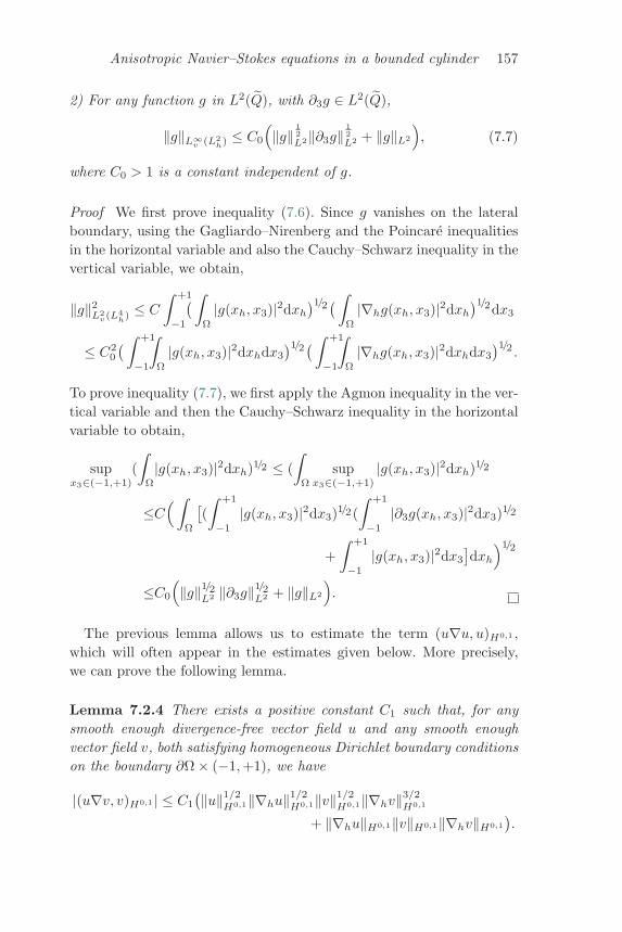
Anisotropic Navier–Stokes equations in a bounded cylinder 157
2) For any function g in L2(Q), with ∂3g ∈ L2(Q),
‖g‖L∞v (L2
h) ≤ C0
(‖g‖ 1
2L2‖∂3g‖
12L2 + ‖g‖L2
), (7.7)
where C0 > 1 is a constant independent of g.
Proof We first prove inequality (7.6). Since g vanishes on the lateralboundary, using the Gagliardo–Nirenberg and the Poincare inequalitiesin the horizontal variable and also the Cauchy–Schwarz inequality in thevertical variable, we obtain,
‖g‖2L2
v(L4h) ≤ C
∫ +1
−1
( ∫Ω
|g(xh, x3)|2dxh
)1/2( ∫Ω
|∇hg(xh, x3)|2dxh
)1/2dx3
≤ C20
( ∫ +1
−1
∫Ω
|g(xh, x3)|2dxhdx3
)1/2( ∫ +1
−1
∫Ω
|∇hg(xh, x3)|2dxhdx3
)1/2 .To prove inequality (7.7), we first apply the Agmon inequality in the ver-tical variable and then the Cauchy–Schwarz inequality in the horizontalvariable to obtain,
supx3∈(−1,+1)
(∫
Ω
|g(xh, x3)|2dxh)1/2 ≤ (∫
Ω
supx3∈(−1,+1)
|g(xh, x3)|2dxh)1/2
≤C(∫
Ω
[(∫ +1
−1
|g(xh, x3)|2dx3)1/2(∫ +1
−1
|∂3g(xh, x3)|2dx3)1/2
+∫ +1
−1
|g(xh, x3)|2dx3
]dxh
)1/2
≤C0
(‖g‖1/2
L2 ‖∂3g‖1/2L2 + ‖g‖L2
).
The previous lemma allows us to estimate the term (u∇u, u)H0,1 ,which will often appear in the estimates given below. More precisely,we can prove the following lemma.
Lemma 7.2.4 There exists a positive constant C1 such that, for anysmooth enough divergence-free vector field u and any smooth enoughvector field v, both satisfying homogeneous Dirichlet boundary conditionson the boundary ∂Ω × (−1,+1), we have
|(u∇v, v)H0,1 | ≤ C1
(‖u‖1/2H0,1‖∇hu‖1/2
H0,1‖v‖1/2H0,1‖∇hv‖3/2
H0,1
+ ‖∇hu‖H0,1‖v‖H0,1‖∇hv‖H0,1
).
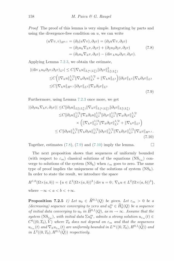
158 M. Paicu & G. Raugel
Proof The proof of this lemma is very simple. Integrating by parts andusing the divergence-free condition on u, we can write
(u∇v, v)H0,1 = (∂3(u∇v), ∂3v) = (∂3u∇v, ∂3v)
= (∂3uh∇hv, ∂3v) + (∂3u3∂3v, ∂3v)
= (∂3uh∇hv, ∂3v) − (div huh∂3v, ∂3v).
(7.8)
Applying Lemma 7.2.3, we obtain the estimate,
|(div huh∂3v,∂3v)L2 | ≤ C‖∇hu‖L∞v (L2
h)‖∂3v‖2L2
v(L4h)
≤C(‖∇hu‖1/2
L2 ‖∇h∂3u‖1/2L2 + ‖∇hu‖L2
)‖∂3v‖L2‖∇h∂3v‖L2
≤C‖∇hu‖H0,1‖∂3v‖L2‖∇h∂3v‖L2
(7.9)
Furthermore, using Lemma 7.2.3 once more, we get
|(∂3uh∇hv, ∂3v)| ≤C‖∂3u‖L2v(L4
h)‖∇hv‖L∞v (L2
h)‖∂3v‖L2v(L4
h)
≤C‖∂3u‖1/2L2 ‖∇h∂3u‖1/2
L2 ‖∂3v‖1/2L2 ‖∇h∂3v‖1/2
L2
×(‖∇hv‖1/2
L2 ‖∇h∂3v‖1/2L2 + ‖∇hv‖L2
)≤ C‖∂3u‖1/2
L2 ‖∇h∂3u‖1/2L2 ‖∂3v‖1/2
L2 ‖∇h∂3v‖1/2L2 ‖∇hv‖H0,1 .
(7.10)
Together, estimates (7.8), (7.9) and (7.10) imply the lemma.
The next proposition shows that sequences of uniformly bounded(with respect to εm) classical solutions of the equations (NSεm) con-verge to solutions of the system (NSh) when εm goes to zero. The sametype of proof implies the uniqueness of the solutions of system (NSh).In order to state the result, we introduce the space
H1,0(Ω×(a, b)) = {u ∈ L2(Ω×(a, b))3 |div u = 0 ; ∇hu ∈ L2(Ω×(a, b))3},where −∞ < a < b < +∞.
Proposition 7.2.5 1) Let u0 ∈ H0,1(Q) be given. Let εm > 0 be a(decreasing) sequence converging to zero and um
0 ∈ H10 (Q) be a sequence
of initial data converging to u0 in H0,1(Q), as m→ ∞. Assume that thesystem (NSεm), with initial data Σum
0 , admits a strong solution uεm(t) ∈
C0((0, T0), V ) where T0 does not depend on εm and that the sequencesuεm
(t) and ∇huεm(t) are uniformly bounded in L∞((0, T0),H0,1(Q)) and
in L2((0, T0),H0,1(Q)) respectively.
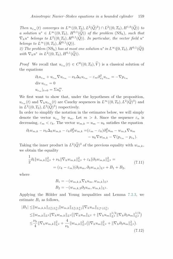
Anisotropic Navier–Stokes equations in a bounded cylinder 159
Then uεm(t) converges in L∞((0, T0), L2(Q)3) ∩ L2((0, T0),H1,0(Q)) to
a solution u∗ ∈ L∞((0, T0), H0,1(Q)) of the problem (NSh), such that∇hu
∗ belongs to L2((0, T0),H0,1(Q)). In particular, the vector field u∗
belongs to L∞((0, T0), H0,1(Q)).2) The problem (NSh) has at most one solution u∗ in L∞((0, T0),H0,1(Q))with ∇hu
∗ in L2((0, T0),H0,1(Q)).
Proof We recall that uεm(t) ∈ C0((0, T0), V ) is a classical solution of
the equations
∂tuεm+ uεm
∇uεm− νhΔhuεm
− εm∂2x3uεm
= −∇pεm
div uεm= 0
uεm|t=0 = Σum
0 .
We first want to show that, under the hypotheses of the proposition,uεm
(t) and ∇huεm(t) are Cauchy sequences in L∞((0, T0), L2(Q)3) and
in L2((0, T0), L2(Q)3) respectively.In order to simplify the notation in the estimates below, we will simplydenote the vector uεm
by um. Let m > k. Since the sequence εn isdecreasing, εm < εk. The vector wm,k = um − uk satisfies the equation
∂twm,k − νhΔhwm,k − εk∂23wm,k =(εm − εk)∂2
3um − wm,k∇um
− uk∇wm,k −∇(pεm− pεk
).
Taking the inner product in L2(Q)3 of the previous equality with wm,k,we obtain the equality
12∂t‖wm,k‖2
L2 + νh‖∇hwm,k‖2L2 + εk‖∂3wm,k‖2
L2 =
= (εk − εm)(∂3um, ∂3wm,k)L2 +B1 +B2,(7.11)
where
B1 = −(wm,k,h∇hum, wm,k)L2
B2 = −(wm,k,3∂3um, wm,k)L2 .
Applying the Holder and Young inequalities and Lemma 7.2.3, weestimate B1 as follows,
|B1| ≤‖wm,k,h‖L2v(L4
h)‖wm,k‖L2v(L4
h)‖∇hum‖L∞v (L2
h)
≤‖wm,k‖L2‖∇hwm,k‖L2
(‖∇hum‖L2 + ‖∇hum‖1/2L2 ‖∇h∂3um‖1/2
L2
)≤νh
4‖∇hwm,k‖2
L2 +4νh
‖wm,k‖2L2
(‖∇hum‖2L2 + ‖∇h∂3um‖2
L2
).
(7.12)
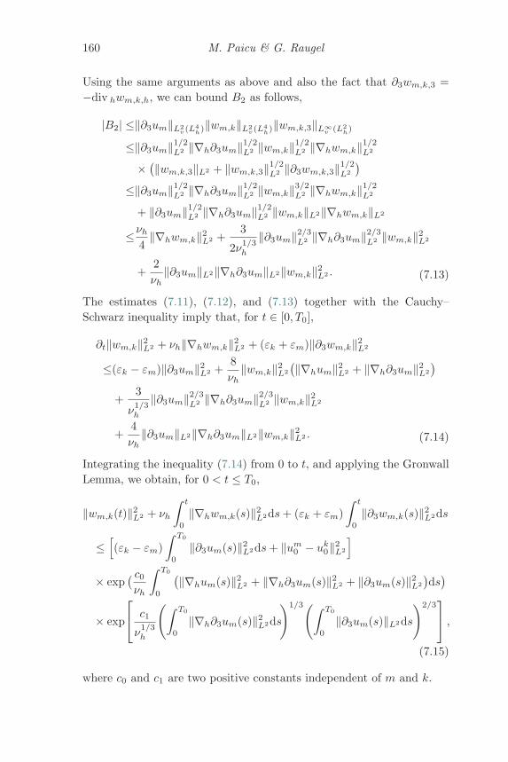
160 M. Paicu & G. Raugel
Using the same arguments as above and also the fact that ∂3wm,k,3 =−div hwm,k,h, we can bound B2 as follows,
|B2| ≤‖∂3um‖L2v(L4
h)‖wm,k‖L2v(L4
h)‖wm,k,3‖L∞v (L2
h)
≤‖∂3um‖1/2L2 ‖∇h∂3um‖1/2
L2 ‖wm,k‖1/2L2 ‖∇hwm,k‖1/2
L2
× (‖wm,k,3‖L2 + ‖wm,k,3‖1/2L2 ‖∂3wm,k,3‖1/2
L2
)≤‖∂3um‖1/2
L2 ‖∇h∂3um‖1/2L2 ‖wm,k‖3/2
L2 ‖∇hwm,k‖1/2L2
+ ‖∂3um‖1/2L2 ‖∇h∂3um‖1/2
L2 ‖wm,k‖L2‖∇hwm,k‖L2
≤νh
4‖∇hwm,k‖2
L2 +3
2ν1/3h
‖∂3um‖2/3L2 ‖∇h∂3um‖2/3
L2 ‖wm,k‖2L2
+2νh
‖∂3um‖L2‖∇h∂3um‖L2‖wm,k‖2L2 . (7.13)
The estimates (7.11), (7.12), and (7.13) together with the Cauchy–Schwarz inequality imply that, for t ∈ [0, T0],
∂t‖wm,k‖2L2 + νh‖∇hwm,k‖2
L2 + (εk + εm)‖∂3wm,k‖2L2
≤(εk − εm)‖∂3um‖2L2 +
8νh
‖wm,k‖2L2
(‖∇hum‖2L2 + ‖∇h∂3um‖2
L2
)+
3
ν1/3h
‖∂3um‖2/3L2 ‖∇h∂3um‖2/3
L2 ‖wm,k‖2L2
+4νh
‖∂3um‖L2‖∇h∂3um‖L2‖wm,k‖2L2 . (7.14)
Integrating the inequality (7.14) from 0 to t, and applying the GronwallLemma, we obtain, for 0 < t ≤ T0,
‖wm,k(t)‖2L2 + νh
∫ t
0
‖∇hwm,k(s)‖2L2ds+ (εk + εm)
∫ t
0
‖∂3wm,k(s)‖2L2ds
≤[(εk − εm)
∫ T0
0
‖∂3um(s)‖2L2ds+ ‖um
0 − uk0‖2
L2
]× exp
( c0νh
∫ T0
0
(‖∇hum(s)‖2L2 + ‖∇h∂3um(s)‖2
L2 + ‖∂3um(s)‖2L2
)ds)
× exp
⎡⎣ c1
ν1/3h
(∫ T0
0
‖∇h∂3um(s)‖2L2ds
)1/3(∫ T0
0
‖∂3um(s)‖L2ds
)2/3⎤⎦ ,
(7.15)
where c0 and c1 are two positive constants independent of m and k.
Anisotropic Navier–Stokes equations in a bounded cylinder 161
Since the sequences uεm(t) and ∇huεm
(t) are uniformly boundedin L∞((0, T0), H0,1(Q)) and in L2((0, T0),H0,1(Q)) respectively, theestimate (7.15) implies that uεm
and ∇huεmare Cauchy sequences
in L∞((0, T0), L2(Q)3) and L2((0, T0), L2(Q)3) respectively. Thus uεm
converges in L∞((0, T0), L2(Q)3) ∩L2((0, T0),H1,0(Q)) to an elementu∗ in this same space. Moreover, u∗ and ∇hu
∗ are bounded inL∞((0, T0),H0,1(Q)) and in L2((0, T0),H0,1(Q)) respectively. The con-vergence in the sense of distributions of uεm
to u∗ and the divergence-freeproperty of the sequence uεm
imply that u∗ is also divergence-free. Fur-thermore, one easily shows that the restriction of u∗ to Q is a weaksolution of the system (NSh). From the equality Σuεm
(t) = uεm(t), it
follows that Σu∗(t) = u∗(t). In particular, u∗3(t) vanishes on Γ0 ∪ Γ1.Finally, we notice that, since uεm
(t) ∈ C0((0, T0), V ) converges inL2((0, T0),H1,0(Q)), u∗(t) satisfies the homogeneous Dirichlet boundarycondition on the lateral boundary ∂Ω× (−1, 1) for almost all t ∈ (0, T0).One proves the uniqueness of the solution u∗ in L∞((0, T0),H0,1(Q))with ∇hu
∗ in L2((0, T0),H0,1(Q)) in the same way as the above Cauchyproperty.
We now state the classical energy estimate which will be widely usedin the subsequent sections.
Lemma 7.2.6 Let uε(t) ∈ C0([0, T0], V ) be the classical solution of theequations (NSε) with initial data uε,0 ∈ V . Then the following estimatesare satisfied, for any t ∈ [0, T0], for any 0 ≤ t0 ≤ t,
‖uε(t)‖2L2 ≤ ‖uε(0)‖2
L2 exp(−2νhλ−10 t), and
νh
∫ t
t0
‖∇huε(s)‖2L2ds+ ε
∫ t
t0
‖∂3uε(s)‖2L2ds
≤ 12‖uε(0)‖2
L2 exp(−2νhλ−10 t0),
(7.16)
where λ0 is the constant from the Poincare inequality.
Proof Since uε ∈ C0([0, T0], V ) is the classical solution of (NSε), we cantake the inner product in L2(Q)3 of the first equation in (NSε) with uε
and integrate by parts. We thus obtain, for 0 ≤ t ≤ T0,
∂t‖uε(t)‖2L2 + 2νh‖∇huε(t)‖2
L2 + 2ε‖∂3uε(t)‖2L2 ≤ 0. (7.17)
Since uε satisfies homogeneous Dirichlet boundary conditions on thelateral boundary, there exists a positive constant λ0 depending only on
162 M. Paicu & G. Raugel
Ω such that
‖uε‖2L2 ≤ λ0‖∇huε‖2
L2 . (7.18)
The inequalities (7.17) and (7.18) imply that, for 0 ≤ t ≤ T0,
∂t‖uε(t)‖2L2 + 2νhλ
−10 ‖uε(t)‖2
L2 ≤ 0.
Integrating the previous inequality and applying the Gronwall Lemma,we obtain the first inequality in (7.16). Integrating now inequality (7.17)from t0 to t and taking into account the first estimate in (7.16), we obtainthe second estimate of (7.16).
We continue this section with an auxiliary proposition, which will beused several times in the proof of global existence of solutions of thesystem (NSε).
Proposition 7.2.7 Let uε ∈ C0([0, T0), V ) be a classical solution of(NSε). Let Tn < T0 be a sequence converging to T0 as n → ∞. If uε(t)is uniformly bounded in L∞((0, Tn),H0,1(Q)) ∩ L2((0, Tn),H0,1(Q)) andif ∇huε and ε∂3uε are uniformly bounded in L2((0, Tn),H0,1(Q)) asn→ ∞, then uε is uniformly bounded in C0([0, Tn], V ) and the classicalsolution uε exists on a time interval [0, Tε) where Tε > T0. In particular,if Tn → ∞ as n→ ∞, then the classical solution uε exists globally.
Proof Let uε ∈ C0([0, T0), V ) be a (local) classical solution of (NSε). Inorder to prove the proposition, we have to show that ∇huε is uniformlybounded in L∞((0, Tn), L2(Q)3) as n → ∞. Since uε is a classical solu-tion, all the a priori estimates made below can be justified. Let P bethe classical Leray projection of L2(Q)3 onto H, where
H = {u ∈ L2(Q)3 |div u = 0 ; γnu|∂Ω×(0,1) = 0 ;
u(xh, x3) = u(xh, x3 + 2)}.
Taking the inner product in L2(Q) of the first equation of (NSε) with−PΔhuε, we obtain the equality
−(∂tuε,Δhuε)+νh‖PΔhuε‖2L2 +ε(∂2
3uε, PΔhuε) = −(uε ·∇uε, PΔhuε).
We remark that, for 0 < t < T0, ∂tuε, ∂3uε and ∂23uε vanish on the
lateral boundary and are periodic in x3. Moreover, the divergence of∂23uε vanishes. These properties imply on the one hand that
−∫
Q
∂tuε · Δhuε dx =∫
Q
∂t∇huε · ∇huε dx =12∂t‖∇huε‖2
L2 .
Anisotropic Navier–Stokes equations in a bounded cylinder 163
On the other hand, we can write, for 0 < t < T0,∫Q
∂23uε · PΔhuεdx =
∫Q
∂23uε · Δhuεdx
= −∫
Q
∂3uε · Δh∂3uεdx = ‖∇h∂3uε‖2L2 .
The previous three equalities imply that, for 0 < t < T0,
∂t‖∇huε‖2L2 +νh‖PΔhuε‖2
L2 +2ε‖∇h∂3uε‖2L2 ≤ 1
νh‖uε ·∇uε‖2
L2 . (7.19)
To estimate the term ‖uε · ∇uε‖2L2 , we write
‖uε · ∇uε‖2L2 =
∫Q
(uε,h · ∇huε + uε,3 · ∂3uε)2dx
≤ 2‖uε,h · ∇huε‖2L2 + 2‖uε,3 · ∂3uε‖2
L2 .
(7.20)
It remains to bound both terms on the right-hand side of the inequality(7.20). Using the Gagliardo–Nirenberg and the Poincare inequalities, wecan write
‖uε,h · ∇huε‖2L2 ≤
∫ 1
−1
‖uε(., x3)‖2L4
h‖∇huε(., x3)‖2
L4h
dx3
≤ c0
(∫ 1
−1
‖uε(., x3)‖L2h‖∇huε(., x3)‖2
L2h‖Dh∇huε(., x3)‖L2
hdx3
+∫ 1
−1
‖uε(., x3)‖L2h‖∇huε(., x3)‖3
L2h
dx3
)≤ c1
(‖uε‖L∞
v (L2h)‖∇huε‖L∞
v (L2h)‖∇huε‖L2‖Dh∇huε‖L2
+ ‖uε‖L∞v (L2
h)‖∇huε‖L∞v (L2
h)‖∇huε‖2L2
).
Applying Lemma 7.2.3 to the previous inequality, we obtain,
‖uε,h · ∇huε‖2L2 ≤c2
(‖uε‖L2 + ‖∂3uε‖1/2
L2 ‖uε‖1/2L2
)×(‖∇huε‖L2 + ‖∂3∇huε‖1/2
L2 ‖∇huε‖1/2L2
)×(‖∇huε‖L2 + ‖Dh∇huε‖L2
)‖∇huε‖L2 .
(7.21)
The classical regularity theorem for the stationary Stokes problem (seefor example Constantin & Foias, 1988; Solonnikov & Scadilov, 1973; orTemam, 1979) implies that there exists a positive constant K0(ε), whichcould depend on ε, such that,
‖Dh∇huε‖L2 ≤ K0(ε)(‖PΔhuε‖L2 +
ε
νh‖∂2
3uε‖L2
). (7.22)
164 M. Paicu & G. Raugel
Using the inequality 2ab ≤ a2 + b2, we deduce from (7.21) and (7.22)that
‖uε,h · ∇huε‖2L2 ≤4c2
(‖uε‖L2 + ‖∂3uε‖L2
)(‖∇huε‖L2 + ‖∂3∇huε‖L2
)×(‖∇huε‖L2 +K0(ε)(‖PΔhuε‖L2 +
ε
νh‖∂2
3uε‖L2))‖∇huε‖L2 ,
and also
2νh
‖uε,h · ∇huε‖2L2 ≤ νh
2‖PΔhuε‖2
L2 +ε2
νh‖∂2
3uε‖2L2 +
νh
2‖∇huε‖2
L2
+ c5K0(ε)2 + 1
ν3h
(‖uε‖2L2 + ‖∂3uε‖2
L2)
× (‖∇huε‖2L2 + ‖∂3∇huε‖2
L2)‖∇huε‖2L2 . (7.23)
Likewise, using the Gagliardo–Nirenberg and the Poincare inequalities,we can write
‖uε,3 · ∂3uε‖2L2 ≤ c1‖uε,3‖L∞
v (L2h)‖∇huε,3‖L∞
v (L2h)‖∂3uε‖L2‖∇h∂3uε‖L2 ,
which implies, due to Lemma 7.2.3, that
‖uε,3 · ∂3uε‖2L2 ≤c2
(‖uε‖L2 + ‖∂3uε,3‖1/2
L2 ‖uε,3‖1/2L2
)×(‖∇huε,3‖L2 + ‖∂3∇huε,3‖1/2
L2 ‖∇huε,3‖1/2L2
)× ‖∂3uε‖L2‖∇h∂3uε‖L2 .
Using the Young inequalities ab ≤ 12a
2 + 12b
2 and ab ≤ 14a
4 + 34b
4/3, wededuce from the previous inequality that
2νh
‖uε,3 · ∂3uε‖2L2 ≤ c6
νh
(‖uε‖L2 + ‖∂3uε,3‖L2
)‖∂3uε‖L2
× (‖∇huε,3‖2L2 + ‖∂3∇huε,3‖2
L2
).
(7.24)
Finally, we deduce from the estimates (7.19), (7.23) and, (7.24) that, for0 ≤ t < T0,
∂t‖∇huε(t)‖2L2 +
νh
2‖PΔhuε‖2
L2
≤ ε2
νh‖∂2
3uε(t)‖2L2 +
νh
2‖∇huε(t)‖2
L2
+ Lε(uε(t))(2c6νh
+ c5(K0(ε)2 + 1)
ν3h
‖∇huε(t)‖2L2
),
(7.25)
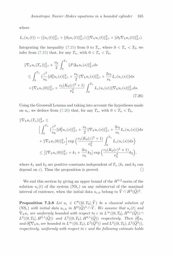
Anisotropic Navier–Stokes equations in a bounded cylinder 165
where
Lε(uε(t)) = (‖uε(t)‖2L2 + ‖∂3uε(t)‖2
L2) (‖∇huε(t)‖2L2 + ‖∂3∇huε(t)‖2
L2).
Integrating the inequality (7.25) from 0 to Tn, where 0 < Tn < T0, weinfer from (7.25) that, for any Tn, with 0 < Tn < T0,
‖∇huε(Tn)‖2L2 +
νh
2
∫ Tn
0
‖PΔhuε(s)‖2L2ds
≤∫ Tn
0
( ε2νh
‖∂23uε(s)‖2
L2 +νh
2‖∇huε(s)‖2
L2 +2c6νh
Lε(uε(s)))ds
+‖∇huε(0)‖2L2 +
c5(K0(ε)2 + 1)ν3
h
∫ Tn
0
Lε(uε(s))‖∇huε(s)‖2L2ds.
(7.26)
Using the Gronwall Lemma and taking into account the hypotheses madeon uε, we deduce from (7.26) that, for any Tn, with 0 < Tn < T0,
‖∇huε(Tn)‖2L2 ≤[ ∫ Tn
0
( ε2νh
‖∂23uε(s)‖2
L2 +νh
2‖∇huε(s)‖2
L2 +2c6νh
Lε(uε(s)))ds
+ ‖∇huε(0)‖2L2
]exp
(c5(K0(ε)2 + 1)ν3
h
∫ Tn
0
Lε(uε(s))ds)
≤ [‖∇huε(0)‖2L2 + k1 +
2c6νh
k2
]exp
(c5(K0(ε)2 + 1)ν3
h
k2
),
where k1 and k2 are positive constants independent of Tn (k1 and k2 candepend on ε). Thus the proposition is proved.
We end this section by giving an upper bound of the H0,2-norm of thesolution uε(t) of the system (NSε) on any subinterval of the maximalinterval of existence, when the initial data uε,0 belong to V ∩H2(Q)3.
Proposition 7.2.8 Let uε ∈ C0([0, T0], V ) be a classical solution of(NSε) with initial data uε,0 in H2(Q)3 ∩ V . We assume that uε(t) and∇huε are uniformly bounded with respect to ε in L∞((0, T0],H0,1(Q)) ∩L2((0, T0],H0,1(Q)) and L2((0, T0),H0,1(Q)) respectively. Then ∂2
3uε
and ∂23∇huε are bounded in L∞((0, T0), L2(Q3)) and L2((0, T0), L2(Q3)),
respectively, uniformly with respect to ε and the following estimate holds
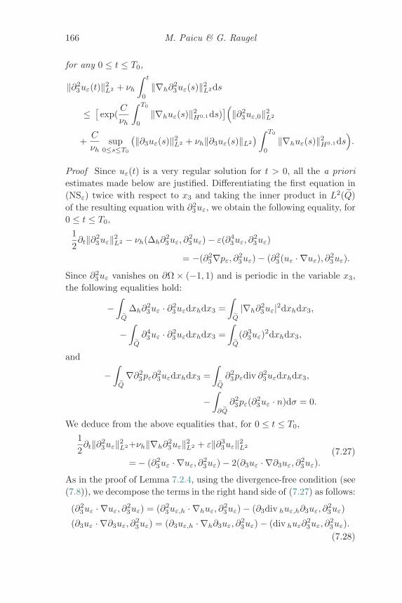
166 M. Paicu & G. Raugel
for any 0 ≤ t ≤ T0,
‖∂23uε(t)‖2
L2 + νh
∫ t
0
‖∇h∂23uε(s)‖2
L2ds
≤ [exp(
C
νh
∫ T0
0
‖∇huε(s)‖2H0,1ds)
](‖∂23uε,0‖2
L2
+C
νhsup
0≤s≤T0
(‖∂3uε(s)‖2L2 + νh‖∂3uε(s)‖L2
) ∫ T0
0
‖∇huε(s)‖2H0,1ds
).
Proof Since uε(t) is a very regular solution for t > 0, all the a prioriestimates made below are justified. Differentiating the first equation in(NSε) twice with respect to x3 and taking the inner product in L2(Q)of the resulting equation with ∂2
3uε, we obtain the following equality, for0 ≤ t ≤ T0,
12∂t‖∂2
3uε‖2L2 − νh(Δh∂
23uε, ∂
23uε) − ε(∂4
3uε, ∂23uε)
= −(∂23∇pε, ∂
23uε) − (∂2
3(uε · ∇uε), ∂23uε).
Since ∂23uε vanishes on ∂Ω × (−1, 1) and is periodic in the variable x3,
the following equalities hold:
−∫
Q
Δh∂23uε · ∂2
3uεdxhdx3 =∫
Q
|∇h∂23uε|2dxhdx3,
−∫
Q
∂43uε · ∂2
3uεdxhdx3 =∫
Q
(∂33uε)2dxhdx3,
and
−∫
Q
∇∂23pε∂
23uεdxhdx3 =
∫Q
∂23pεdiv ∂2
3uεdxhdx3,
−∫
∂Q
∂23pε(∂2
3uε · n)dσ = 0.
We deduce from the above equalities that, for 0 ≤ t ≤ T0,12∂t‖∂2
3uε‖2L2+νh‖∇h∂
23uε‖2
L2 + ε‖∂33uε‖2
L2
= − (∂23uε · ∇uε, ∂
23uε) − 2(∂3uε · ∇∂3uε, ∂
23uε).
(7.27)
As in the proof of Lemma 7.2.4, using the divergence-free condition (see(7.8)), we decompose the terms in the right hand side of (7.27) as follows:
(∂23uε · ∇uε, ∂
23uε) = (∂2
3uε,h · ∇huε, ∂23uε) − (∂3div huε,h∂3uε, ∂
23uε)
(∂3uε · ∇∂3uε, ∂23uε) = (∂3uε,h · ∇h∂3uε, ∂
23uε) − (div huε∂
23uε, ∂
23uε).(7.28)
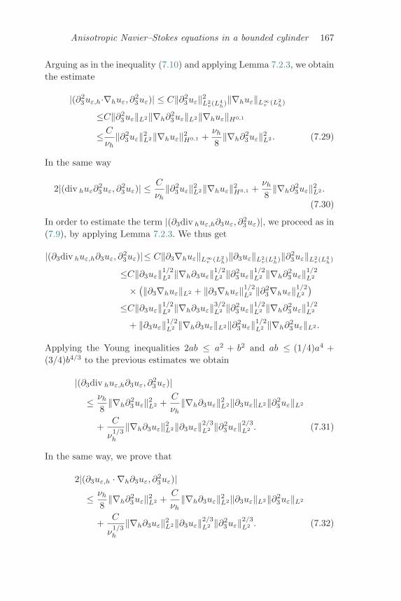
Anisotropic Navier–Stokes equations in a bounded cylinder 167
Arguing as in the inequality (7.10) and applying Lemma 7.2.3, we obtainthe estimate
|(∂23uε,h·∇huε, ∂
23uε)| ≤ C‖∂2
3uε‖2L2
v(L4h)‖∇huε‖L∞
v (L2h)
≤C‖∂23uε‖L2‖∇h∂
23uε‖L2‖∇huε‖H0,1
≤ C
νh‖∂2
3uε‖2L2‖∇huε‖2
H0,1 +νh
8‖∇h∂
23uε‖2
L2 . (7.29)
In the same way
2|(div huε∂23uε, ∂
23uε)| ≤ C
νh‖∂2
3uε‖2L2‖∇huε‖2
H0,1 +νh
8‖∇h∂
23uε‖2
L2 .
(7.30)
In order to estimate the term |(∂3div huε,h∂3uε, ∂23uε)|, we proceed as in
(7.9), by applying Lemma 7.2.3. We thus get
|(∂3div huε,h∂3uε, ∂23uε)|≤ C‖∂3∇huε‖L∞
v (L2h)‖∂3uε‖L2
v(L4h)‖∂2
3uε‖L2v(L4
h)
≤C‖∂3uε‖1/2L2 ‖∇h∂3uε‖1/2
L2 ‖∂23uε‖1/2
L2 ‖∇h∂23uε‖1/2
L2
× (‖∂3∇huε‖L2 + ‖∂3∇huε‖1/2L2 ‖∂2
3∇huε‖1/2L2
)≤C‖∂3uε‖1/2
L2 ‖∇h∂3uε‖3/2L2 ‖∂2
3uε‖1/2L2 ‖∇h∂
23uε‖1/2
L2
+ ‖∂3uε‖1/2L2 ‖∇h∂3uε‖L2‖∂2
3uε‖1/2L2 ‖∇h∂
23uε‖L2 .
Applying the Young inequalities 2ab ≤ a2 + b2 and ab ≤ (1/4)a4 +(3/4)b4/3 to the previous estimates we obtain
|(∂3div huε,h∂3uε, ∂23uε)|
≤ νh
8‖∇h∂
23uε‖2
L2 +C
νh‖∇h∂3uε‖2
L2‖∂3uε‖L2‖∂23uε‖L2
+C
ν1/3h
‖∇h∂3uε‖2L2‖∂3uε‖2/3
L2 ‖∂23uε‖2/3
L2 . (7.31)
In the same way, we prove that
2|(∂3uε,h · ∇h∂3uε, ∂23uε)|
≤ νh
8‖∇h∂
23uε‖2
L2 +C
νh‖∇h∂3uε‖2
L2‖∂3uε‖L2‖∂23uε‖L2
+C
ν1/3h
‖∇h∂3uε‖2L2‖∂3uε‖2/3
L2 ‖∂23uε‖2/3
L2 . (7.32)
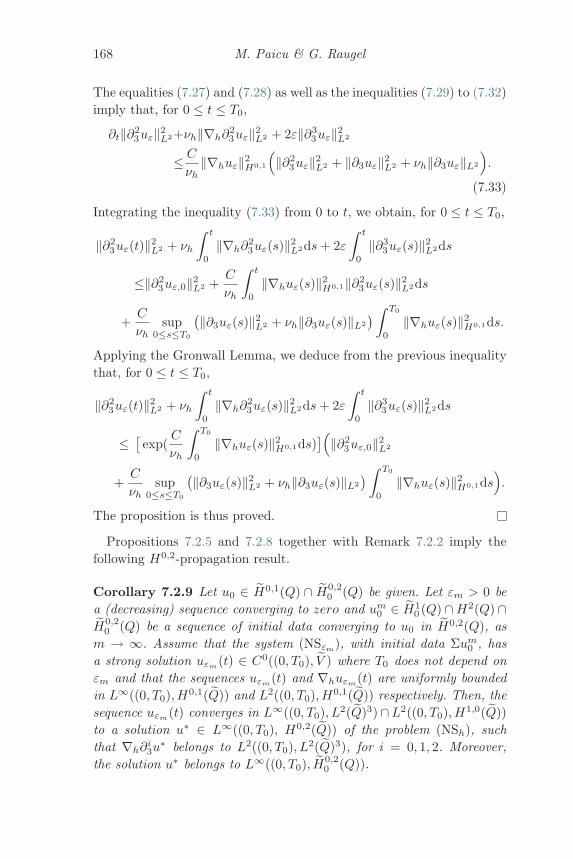
168 M. Paicu & G. Raugel
The equalities (7.27) and (7.28) as well as the inequalities (7.29) to (7.32)imply that, for 0 ≤ t ≤ T0,
∂t‖∂23uε‖2
L2+νh‖∇h∂23uε‖2
L2 + 2ε‖∂33uε‖2
L2
≤ C
νh‖∇huε‖2
H0,1
(‖∂2
3uε‖2L2 + ‖∂3uε‖2
L2 + νh‖∂3uε‖L2
).
(7.33)
Integrating the inequality (7.33) from 0 to t, we obtain, for 0 ≤ t ≤ T0,
‖∂23uε(t)‖2
L2 + νh
∫ t
0
‖∇h∂23uε(s)‖2
L2ds+ 2ε∫ t
0
‖∂33uε(s)‖2
L2ds
≤‖∂23uε,0‖2
L2 +C
νh
∫ t
0
‖∇huε(s)‖2H0,1‖∂2
3uε(s)‖2L2ds
+C
νhsup
0≤s≤T0
(‖∂3uε(s)‖2L2 + νh‖∂3uε(s)‖L2
) ∫ T0
0
‖∇huε(s)‖2H0,1ds.
Applying the Gronwall Lemma, we deduce from the previous inequalitythat, for 0 ≤ t ≤ T0,
‖∂23uε(t)‖2
L2 + νh
∫ t
0
‖∇h∂23uε(s)‖2
L2ds+ 2ε∫ t
0
‖∂33uε(s)‖2
L2ds
≤ [exp(
C
νh
∫ T0
0
‖∇huε(s)‖2H0,1ds)
](‖∂23uε,0‖2
L2
+C
νhsup
0≤s≤T0
(‖∂3uε(s)‖2L2 + νh‖∂3uε(s)‖L2
) ∫ T0
0
‖∇huε(s)‖2H0,1ds
).
The proposition is thus proved.
Propositions 7.2.5 and 7.2.8 together with Remark 7.2.2 imply thefollowing H0,2-propagation result.
Corollary 7.2.9 Let u0 ∈ H0,1(Q) ∩ H0,20 (Q) be given. Let εm > 0 be
a (decreasing) sequence converging to zero and um0 ∈ H1
0 (Q) ∩H2(Q) ∩H0,2
0 (Q) be a sequence of initial data converging to u0 in H0,2(Q), asm → ∞. Assume that the system (NSεm), with initial data Σum
0 , hasa strong solution uεm
(t) ∈ C0((0, T0), V ) where T0 does not depend onεm and that the sequences uεm
(t) and ∇huεm(t) are uniformly bounded
in L∞((0, T0),H0,1(Q)) and L2((0, T0),H0,1(Q)) respectively. Then, thesequence uεm
(t) converges in L∞((0, T0), L2(Q)3)∩L2((0, T0),H1,0(Q))to a solution u∗ ∈ L∞((0, T0), H0,2(Q)) of the problem (NSh), suchthat ∇h∂
i3u
∗ belongs to L2((0, T0), L2(Q)3), for i = 0, 1, 2. Moreover,the solution u∗ belongs to L∞((0, T0), H0,2
0 (Q)).
Anisotropic Navier–Stokes equations in a bounded cylinder 169
Proof Let u0 ∈ H0,1(Q)∩ H0,20 (Q) be given. We notice that, by Remark
7.2.2, there exists a sequence um0 ∈ H1
0 (Q) ∩H2(Q) ∩ H0,20 (Q) of initial
data converging to u0 in H0,2(Q), as m→ ∞. Let um0 be such a sequence.
As we have remarked in the introduction, Σum0 belongs to H2(Q)3 and
∂3um0,h vanishes on Γ0 ∪ Γ1. By Proposition 7.2.8, the classical solution
uεmof (NSεm) is more regular in the sense that ∂2
3uεm(respectively
∇h∂23uεm
) is uniformly bounded in L∞((0, T0), L2(Q)3) (respectively inL2((0, T0), L2(Q)3). Thus the limit ∂2
3u∗ belongs to L∞((0, T0), L2(Q)3)
and ∇h∂23u
∗ belongs to L2((0, T0), L2(Q)3).
7.3 Global existence results for small initial data
We begin with the simplest result.
Theorem 7.3.1 There exists a positive constant c0 such that, if u0
belongs to H0,1(Q) and ‖u0‖H0,1 ≤ c0νh, then the system (NSh) admitsa (unique) global solution u(t), with u(0) = u0, such that
u ∈ L∞(R+, H0,1(Q)) and ∂3∇hu ∈ L2(R+, L
2(Q)3).
Proof According to the strategy explained in the introduction andaccording to Proposition 7.2.5, it is sufficient to prove that there existsa positive constant c1 such that if uε(0) = w0 belongs to H1
0,per(Q) andsatisfies
‖w0‖H0,1 ≤ c1νh,
then, for any ε > 0, the equations (NSε) admit a unique global solutionuε(t) ∈ C0([0,+∞), V ) with uε(0) = w0 and moreover, uε and ∂3∇huε
are uniformly bounded (with respect to ε) in L∞((0,+∞),H0,1(Q)) andL2((0,+∞), L2(Q)3).Let uε be the local solution of the equations (NSε) with uε(0) = w0.Since uε is a classical solution on the maximal interval of existence, allthe a priori estimates made below can be justified rigorously. Differenti-ating the first equation in (NSε) with respect to x3 and taking the innerproduct in L2(Q)3 with ∂3uε, we obtain, for 0 ≤ t ≤ Tε, where Tε > 0is the maximal time of existence,
12∂t‖∂3uε‖2
L2−νh(Δh∂3uε, ∂3uε) − ε(∂33uε, ∂3uε)
= −(∇∂3pε, ∂3uε) − (∂3(uε∇uε), ∂3uε).(7.34)
170 M. Paicu & G. Raugel
Since uε and hence ∂3uε vanish on the lateral boundary ∂Ω × (−1, 1)and uε and pε are periodic in the vertical variable,
−∫
Q
Δh∂3uε · ∂3uεdxhdx3 =∫
Q
|∇h∂3uε|2dxhdx3
−∫
Q
∂33uε · ∂3uεdxhdx3 =
∫Q
(∂23uε)2dxhdx3,
(7.35)
and
−∫
Q
∇∂3pε∂3uεdxhdx3 =∫
Q
∂3pεdiv ∂3uεdxhdx3
−∫
∂Q
∂3pε(∂3uε · n)dσ = 0 .(7.36)
The equalities (7.34), (7.35), and (7.36) together with Lemma 7.2.4 implythat, for 0 ≤ t ≤ Tε,
∂t‖∂3uε‖2L2 + 2νh‖∇h∂3uε|‖2
L2 + 2ε‖∂23uε‖2
L2
≤ 4C1‖uε‖H0,1‖∇huε‖2H0,1 . (7.37)
We deduce from the estimates (7.17) and (7.37) that, for 0 ≤ t ≤ Tε,
∂t
(‖uε‖2L2 + ‖∂3uε‖2
L2
)+ 2νh
(‖∇huε|‖2L2 + ‖∇h∂3uε|‖2
L2
)+ 2ε
(‖∂3uε‖2L2 + ‖∂2
3uε‖2L2
)≤ 8C1‖uε‖H0,1
(‖∇huε|‖2L2 + ‖∇h∂3uε|‖2
L2
).
(7.38)
Suppose now that the initial condition uε(0) = w0 is small enough inthe sense that
‖w0‖H0,1 ≤ νh
32C1.
Then, by continuity, there exists a time interval [0, τε) such that, fort ∈ [0, τε), ‖uε(t)‖H0,1 < νh/(8C1). If τε < Tε, then ‖uε(τε)‖H0,1 =νh/(8C1). Assume now that τε < Tε. If t belongs to the time interval[0, τε], we deduce from the inequality (7.38) that
∂t
(‖uε‖2L2 + ‖∂3uε‖2
L2
)+ νh
(‖∇huε‖2L2 + ‖∇h∂3uε‖2
L2
)+ 2ε
(‖∂3uε‖2L2 + ‖∂2
3uε‖2L2
) ≤ 0. (7.39)
Anisotropic Navier–Stokes equations in a bounded cylinder 171
Integrating the inequality (7.39) from 0 to t, we obtain that, for t ≤ τε,
‖uε(t)‖2L2+‖∂3uε(t)‖2
L2 + νh
∫ t
0
(‖∇huε(s)‖2L2 + ‖∇h∂3uε(s)‖2
L2
)ds
+ 2ε∫ t
0
(‖∂3uε(s)‖2L2 + ‖∂2
3uε(s)‖2L2
)ds ≤ ‖w0‖2
L2 + ‖∂3w0‖2L2 .
(7.40)
The estimate (7.40) implies that, for t ≤ τε,
‖uε(t)‖H0,1 ≤ νh
16C1.
In particular, ‖uε(τε)‖H0,1 ≤ νh/(16C1), which contradicts the definitionof τε. Thus τε = Tε and one deduces from (7.40) that, for 0 ≤ t < Tε,
‖uε(t)‖2L2+‖∂3uε(t)‖2
L2 + νh
∫ Tε
0
(‖∇huε(s)‖2L2 + ‖∇h∂3uε(s)‖2
L2
)ds
+ 2ε∫ Tε
0
(‖∂3uε(s)‖2L2 + ‖∂2
3uε(s)‖2L2
)ds ≤ ‖w0‖2
L2 + ‖∂3w0‖2L2 .
To prove that uε(t) exists globally, that is, that Tε = +∞, it remains toshow that ‖∇huε(t)‖L2 is uniformly bounded with respect to t ∈ [0, Tε).But this property is a direct consequence of Proposition 7.2.7, and soTheorem 7.3.1 is proved.
A more careful analysis allows us to prove the following more refinedglobal existence result.
Theorem 7.3.2 There exist positive constants c0 and c∗0 such that, ifu0 belongs to H0,1(Q) and satisfies the following smallness condition
‖∂3u0‖12L2(Ω)‖u0‖
12L2(Ω) exp(
c0‖u0‖2L2
ν2h
) ≤ c∗0νh,
then the system (NSh) with u(0) = u0 admits a (unique) global solutionu(t), such that
u ∈ L∞(R+, H0,1(Q)) and ∂3∇hu ∈ L2(R+;L2(Q)3).
Proof As in the proof of Theorem 7.3.1, it is sufficient to prove that thereexist positive constants c1 and c∗1 such that if uε(0) = w0 belongs to
172 M. Paicu & G. Raugel
H10,per(Q) and satisfies
‖∂3w0‖12L2(Ω)‖w0‖
12L2(Ω) exp(c1
‖w0‖2L2
ν2h
) ≤ c∗1νh,
then, for any ε > 0, the equations (NSε) with uε(0) = w0 admit a uniqueglobal solution uε(t) ∈ C0([0,+∞), V ) and moreover, uε and ∇huε areuniformly bounded (with respect to ε) in L∞((0,+∞),H0,1(Q)) andL2((0,+∞),H0,1(Q)).
Now let uε be the local solution of the equations (NSε) with uε(0) = w0
and let Tε > 0 be the maximal time of existence. As in the proof ofTheorem 7.3.1, uε satisfies the equality (7.34). But here, in order toestimate the term (∂3(uε∇uε), ∂3uε), we take into account the estimates(7.9) and (7.10), instead of applying Lemma 7.2.4 directly. The equalities(7.34), (7.35), (7.36), (7.8) and, the estimates (7.9) and (7.10) imply that,for 0 ≤ t < Tε,
∂t‖∂3uε‖2L2 + 2νh‖∇h∂3uε‖2
L2 + 2ε‖∂23uε‖2
L2
≤ C2
(‖∇huε‖1/2L2 ‖∂3uε‖L2‖∇h∂3uε‖3/2
L2 +
+ ‖∇huε‖L2‖∂3uε‖L2‖∇h∂3uε‖L2
).
(7.41)
Using the Young inequalities ab ≤ 34a
43 + 1
4b4 and ab ≤ 1
2a2 + 1
2b2, we
get the following estimates,
C2‖∇huε‖1/2L2 ‖∂3uε‖L2‖∇h∂3uε‖3/2
L2
≤ 27C42
32ν3h
‖∇huε‖2L2‖∂3uε‖4
L2 +νh
2‖∇h∂3uε‖2
L2
(7.42)
and
C2‖∇huε‖L2‖∂3uε‖L2‖∇h∂3uε‖L2
≤ C22
2νh‖∇huε‖2
L2‖∂3uε‖2L2 +
νh
2‖∇h∂3uε‖2
L2 . (7.43)
From the estimates (7.41), (7.42), and (7.43), we deduce that, for0 ≤ t < Tε,
ddt
‖∂3uε(t)‖2L2 + νh‖∇h∂3uε(t)‖2
L2 + 2ε‖∂23uε‖2
L2
≤ C3
( 1νh
‖∇huε‖2L2‖∂3uε‖2
L2 +1ν3
h
‖∇huε‖2L2‖∂3uε‖4
L2
), (7.44)
Anisotropic Navier–Stokes equations in a bounded cylinder 173
where C3 = max (C22/2, 27C4
2/32). The inequality (7.44) shows that, ifthere exists τε < Tε such that ‖∂3uε(τε)‖2
L2 vanishes, then ‖∂3uε(t)‖2L2
is identically equal to zero for τε ≤ t < Tε.
On the time interval [0, τε), the inequality
ddt
‖∂3uε(t)‖2L2 ≤ C3
( 1νh
‖∇huε‖2L2‖∂3uε‖2
L2
+1ν3
h
‖∇huε‖2L2‖∂3uε‖4
L2
) (7.45)
can be written as
− ddt
‖∂3uε(t)‖−2L2 ≤ C3
νh‖∇huε‖2
L2‖∂3uε‖−2L2 +
C3
ν3h
‖∇huε‖2L2
or also
− ddt
(‖∂3uε‖−2
L2 exp(C3
νh
∫ t
0
‖∇huε(s)‖2L2ds)
)≤ C3
ν3h
‖∇huε(t)‖2L2 exp(
C3
νh
∫ t
0
‖∇huε(s)‖2L2ds).
Integrating this inequality from 0 to t, we obtain, for 0 ≤ t < τε,
‖∂3w0‖−2L2 − ‖∂3uε(t)‖−2
L2 exp(C3
νh
∫ t
0
‖∇huε(s)‖2L2ds)
≤ C3
ν3h
∫ t
0
‖∇huε(s)‖2L2ds× exp(
C3
νh
∫ t
0
‖∇huε(s)‖2L2ds). (7.46)
The second energy estimate in Lemma 7.2.6 and the inequality (7.46)imply that, for 0 ≤ t < τε,
‖∂3w0‖−2L2 − C3
ν4h
‖w0‖2L2 exp(
C3‖w0‖2L2
ν2h
) ≤ ‖∂3uε(t)‖−2L2 exp(
C3‖w0‖2L2
ν2h
).
Thus, if we assume that,
‖∂3w0‖−2L2 − C3‖w0‖2
L2
ν4h
exp(C3‖w0‖2
L2
ν2h
) > 0,
that is,
‖∂3w0‖1/2L2 ‖w0‖1/2
L2 exp(C3‖w0‖2
L2
4ν2h
) < C−1/43 νh,
174 M. Paicu & G. Raugel
then we get the following uniform bound, for 0 ≤ t < τε,
‖∂3uε(t)‖2L2
≤ exp(C3‖w0‖2
L2
ν2h
)(‖∂3w0‖−2
L2 − C3
ν4h
‖w0‖2L2 exp(
C3‖w0‖2L2
ν2h
))−1
.
(7.47)
Let us denote by B0 the right-hand side of this inequality. Integratingthe estimate (7.44) from 0 to t and taking into account the second energyestimate in Lemma 7.2.6 as well as the estimate (7.47) and the definitionof τε, we at once obtain the following inequality, for any 0 ≤ t < Tε,
νh
∫ t
0
‖∇h∂3uε(s)‖2L2ds+ 2ε
∫ t
0
‖∂23uε(s)‖2
L2ds
≤ C3
νhB2
0
(1 +
1ν2
h
B20
) ∫ t
0
‖∇huε(s)‖2L2ds
≤ C3
2ν2h
B20
(1 +
1ν2
h
B20
)‖w0‖2L2 .
To prove that uε(t) exists globally, that is, that Tε = +∞, it remains toshow that ‖∇huε(t)‖L2 is uniformly bounded with respect to t ∈ [0, Tε).As in the proof of Theorem 7.3.1, this property is a direct consequenceof Proposition 7.2.7. Theorem 7.3.2 is thus proved.
Remark 7.3.3 The previous theorem allows us to take large initial datain the following sense. For example, we can take u0 ∈ H0,1(Q) such that
‖u0‖L2(Q) ≤ Cηα
and
‖∂3u0‖L2(Q) ≤ Cη−α,
where η is a small positive constant going to 0 and C > 0 is anappropriate positive constant.
Remark 7.3.4 Let us come back to the inequality (7.45). If we set
y(t) =νh
2+
1νh
‖∂3uε(t)‖2L2 and g(t) =
C3
νh‖∇huε(t)‖2
L2 ,
then the inequality (7.45) becomes, for 0 ≤ t < τε,
dydt
(t) ≤ g(t) y2(t).
Anisotropic Navier–Stokes equations in a bounded cylinder 175
Integrating this inequality from 0 to t, for 0 ≤ t < τε, we get
− 1y(t)
+1
y(0)≤∫ t
0
g(s) ds,
hence
y(t) ≤ y(0)
1 − y(0)∫ t
0g(s)ds
,
as long as 1 − y(0)∫ t
0g(s) ds > 0. This implies that
νh
2+
1νh
‖∂3uε(t)‖2L2 ≤
(νh
2+
1νh
‖∂3uε(0)‖2L2
)×(
1 − C3
νh
∫ t
0
‖∇huε(s)‖2L2 ds
(νh
2+
1νh
‖∂3uε(0)‖2L2
))−1
.
(7.48)
Inequality (7.48) and Lemma 7.2.6 imply that
νh
2+
1νh
‖∂3uε(t)‖2L2 ≤
(νh
2+
1νh
‖∂3uε(0)‖2L2
)×(
1 − C3
2ν2h
‖uε(0)‖2L2
(νh
2+
1νh
‖∂3uε(0)‖2L2
))−1
.
Thus, if
C3‖uε(0)‖2L2
(νh
2+
1νh
‖∂3uε(0)‖2L2
) ≤ ν2h, (7.49)
we obtain the following uniform bound, for 0 ≤ t < τε,
νh
2+
1νh
‖∂3uε(t)‖2L2 ≤ 2
(νh
2+
1νh
‖∂3uε(0)‖2L2
).
As in the proof of Theorem 7.3.2, we deduce that, under the condition(7.49), the solution uε(t) exists globally.
Theorems 7.3.1 and 7.3.2 together with Corollary 7.2.9 imply, at once,the following result of propagation of regularity.
Corollary 7.3.5 Under the hypotheses of Theorem 7.3.1 or 7.3.2, if inaddition the initial condition u0 belongs to H0,2
0 (Q), then the solution u
of system (NSh) with u(0) = u0 belongs to L∞(R+, H0,20 (Q)) and ∂2
3∇hu
belongs to L2(R+, L2(Q)3).
176 M. Paicu & G. Raugel
7.4 The case of general initial data
In this section, we want to prove the local existence of the solution u(t)of the equations (NSh), when the initial data are not necessarily small.
Theorem 7.4.1 Let U0 be given in H0,1(Q). There exist a positive timeT0 and a positive constant η such that, if u0 belongs to H0,1(Q) and‖U0 − u0‖H0,1 ≤ η, then the system (NSh) admits a (unique) strongsolution u(t), with u(0) = u0, such that
u ∈ L∞((0, T0), H0,1(Q)) and ∂3∇hu ∈ L2((0, T0), L2(Q)3).
Proof According to the strategy explained in the introduction andaccording to Proposition 7.2.5, it is sufficient to prove that there existpositive constants η and T0 such that, if uε(0) = v0 belongs to H1
0,per(Q)and satisfies
‖v0 − ΣU0‖H0,1(Q) ≤ η, (7.50)
then, for any ε > 0 small enough, the equations (NSε) admit a unique(local) solution uε(t) ∈ C0([0, T0], V ) with uε(0) = v0 and more-over, uε and ∂3∇huε are uniformly bounded with respect to ε inL∞((0, T0),H0,1(Q)) and L2((0, T0), L2(Q)3).Let uε(t) be the strong solution of the equations (NSε) with initial datauε(0) = v0 ∈ H1
0,per(Q) satisfying the condition (7.50). Let Tε > 0 bethe maximal time of existence of this solution. The proof of Theorem7.3.2 and Remark 7.3.4 show that, if
C3
νh
∫ τ
0
‖∇huε(s)‖2L2ds
(νh
2+
1νh
‖∂3uε(0)‖2L2
)< 1,
then Tε > τ .It is thus sufficient to show that, for η > 0 small enough, there exists apositive constant T0 such that, for any ε > 0, the strong solution uε of(NSε) satisfies the inequality
C3
νh
∫ T0
0
‖∇huε(s)‖2L2 ds
(νh
2+
1νh
‖∂3v0‖2L2
)<
12. (7.51)
Actually, property (7.51) will be proved if we show that, for any positivenumber δ, there exist two positive numbers T0 = T0(δ) and η0 = η0(δ)such that ∫ T0
0
‖∇huε(s)‖2L2ds ≤ 4δ. (7.52)
Anisotropic Navier–Stokes equations in a bounded cylinder 177
The remaining part of the proof consists in showing (7.52). Notice thatLemma 7.2.6 gives us an estimate of the quantity
∫ t
0‖∇huε(s)‖2
L2ds,which we have used in the proofs of Theorems 7.3.1 and 7.3.2. Unfor-tunately, here the initial data uε(0) = v0 are not necessarily small. Inorder to prove (7.52), we write the solution uε as
uε = vε + zε,
where vε is the solution of the linear Stokes problem
(LSε)
⎧⎪⎪⎪⎪⎪⎪⎪⎨⎪⎪⎪⎪⎪⎪⎪⎩
∂tvε − νhΔhvε − ε∂2x3vε = −∇qε in Q, t > 0,
div vε = 0 in Q, t > 0,
vε|∂Ω×(−1,1) = 0, t > 0,
vε(xh, x3) = vε(xh, x3 + 2), t > 0,
vε|t=0 = v0,
and where zε is the solution of the following auxiliary nonlinear system
(Zε)
⎧⎪⎪⎪⎪⎪⎪⎪⎨⎪⎪⎪⎪⎪⎪⎪⎩
∂tzε+(zε+ vε)∇(zε+ vε)− νhΔhzε− ε∂2x3zε = −∇q∗ε in Q, t > 0,
div zε = 0 in Q, t > 0,
zε|∂Ω×(−1,1) = 0 , t > 0,
zε(xh, x3) = zε(xh, x3 + 2), t > 0,
zε|t=0 = 0.
The Stokes problem (LSε) admits a unique (global) classical solution vε
in C0([0,+∞), V ). Lemma 7.2.6 implies that, for any t ≥ 0,
‖vε(t)‖2L2 + νh
∫ t
0
‖∇hvε(s)‖2L2ds+ ε
∫ t
0
‖∂3vε(s)‖2L2ds ≤ ‖v0‖2
L2 .
(7.53)Arguing as in the proofs of Theorems 7.3.1 and 7.3.2, one at once showsthat, for t ≥ 0,
‖∂3vε(t)‖2L2 + νh
∫ t
0
‖∇h∂3vε(s)‖2L2ds+ ε
∫ t
0
‖∂23vε(s)‖2
L2ds ≤ ‖∂3v0‖2L2 .
(7.54)
Notice that (Zε) also admits a unique classical solution zε∈C0([0, Tε),V ),where Tε is the maximal time of existence of uε.We will prove that, for η > 0 small enough, there exists a T0 > 0,independent of ε, but depending on U0, such that∫ T0
0
‖∇hvε(s)‖2L2ds ≤ δ and
∫ T0
0
‖∇hzε(s)‖2L2ds ≤ δ . (7.55)
178 M. Paicu & G. Raugel
We introduce a positive number δ0 ≤ δ, which will be made more preciselater. In order to prove the first inequality of (7.55), we proceed as followsby decomposing the linear Stokes problem (LSε) into two auxiliary linearsystems, the first one with very regular initial data and the second onewith small initial data. We recall that P is the classical Leray projector.Let A0 be the Stokes operator A0 = −PΔ with homogeneous Dirichletboundary conditions on ∂Ω × (−1, 1) and periodic boundary conditionsin the vertical variable. The spectrum of A0 consists of a non-decreasingsequence of eigenvalues
0 < λ0 < λ1 ≤ λ2 ≤ · · · ≤ λm ≤ · · · ,which tends to infinity as m tends to infinity. We denote by Pk theprojection onto the space generated by the eigenfunctions associatedto the first k eigenvalues of the operator A0. There exists an integerk0 = k0(δ0) such that,
‖(I − Pk)ΣU0‖2L2 ≤ δ0νh
16∀k ≥ k0. (7.56)
If v0 ∈ H10,per(Q) satisfies condition (7.50), property (7.56) implies that
‖(I−Pk0)v0‖2L2 ≤2‖(I−Pk0)U0‖2
L2+2‖(I−Pk0)(U0−v0)‖2L2 ≤ δ0νh
8+2η2.
On the other hand, the following obvious estimate holds,
‖Pk0v0‖2H1(Q)
≤ λk0+1‖v0‖2L2 ≤ λk0+1(2‖U0‖2
L2 + 2η2). (7.57)
We next decompose vε into the sum vε = v1,ε + v2,ε where v1,ε is thesolution of the Stokes problem
(LS1,ε)
⎧⎪⎪⎪⎪⎪⎪⎪⎨⎪⎪⎪⎪⎪⎪⎪⎩
∂tv1,ε − νhΔhv1,ε − ε∂2x3v1,ε = −∇q1,ε in Q, t > 0,
div v1,ε = 0 in Q, t > 0,
v1,ε|∂Ω×(−1,1) = 0, t > 0,
v1,ε(xh, x3) = v1,ε(xh, x3 + 2), t > 0,
v1,ε|t=0 = Pk0v0,
and v2,ε is the solution of the Stokes problem
(LS2,ε)
⎧⎪⎪⎪⎪⎪⎪⎪⎨⎪⎪⎪⎪⎪⎪⎪⎩
∂tv2,ε − νhΔhv2,ε − ε∂2x3v2,ε = −∇q2,ε in Q, t > 0,
div v2,ε = 0 in Q, t > 0,
v2,ε|∂Ω×(−1,1) = 0, t > 0,
v2,ε(xh, x3) = v2,ε(xh, x3 + 2), t > 0,
v2,ε|t=0 = (I − Pk0)v0.
Anisotropic Navier–Stokes equations in a bounded cylinder 179
From Lemma 7.2.6 we deduce that, for t ≥ 0,
‖v2,ε(t)‖2L2 + νh
∫ t
0
‖∇hv2,ε(s)‖2L2ds+ ε
∫ t
0
‖∂3v2,ε(s)‖2L2ds
≤‖(I − Pk0)v0‖2L2 ≤ δ0νh
8+ 2η2.
(7.58)
Hence, if η2 ≤ δ0νh/16, we obtain, for any t ≥ 0,∫ t
0
‖∇hv2,ε(s)‖2L2ds ≤ δ0
8+
2η2
νh≤ δ0
4. (7.59)
In order to get an upper bound of the term∫ t
0‖∇hv1,ε(s)‖2
L2ds, we firstestimate ‖∇hv1,ε(s)‖2
L2 for any s ≥ 0. As in the proof of Proposition7.2.7, we take the inner product in L2(Q)3 of the first equation of (LS1,ε)with −PΔhv1,ε. Arguing as in the proof of Proposition 7.2.7, we obtain,for any t ≥ 0,
∂t‖∇hv1,ε‖2L2 + νh‖PΔhv1,ε‖2
L2 + 2ε‖∇h∂3v1,ε‖2L2 ≤ 0.
Integrating the above inequality between 0 and t and taking into accountthe estimate (7.57), we obtain, for t ≥ 0,
‖∇hv1,ε(t)‖2L2 + νh
∫ t
0
‖PΔhv1,ε(s)‖2L2ds+ 2ε
∫ t
0
‖∇h∂3v1,ε(s)‖2L2ds
≤‖Pk0v0‖2H1(Q)
≤ λk0+1(2‖U0‖2L2 + 2η2).
From the above inequality, we deduce that, for t ≥ 0,∫ t
0
‖∇hv1,ε(s)‖2L2ds ≤ tλk0+1(2‖U0‖2
L2+2η2) ≤ tλk0+1(2‖U0‖2L2+
δ0νh
8),
and thus, if
0 < T0 ≤ δ04λk0+1
(2‖U0‖2L2 +
δ0νh
8)−1, (7.60)
then ∫ T0
0
‖∇hv1,ε(s)‖2L2 ds ≤ δ0
4. (7.61)
Inequalities (7.59) and (7.61) imply that, if η2 ≤ δ0νh/16 and if thecondition (7.60) holds, then∫ T0
0
‖∇hvε(s)‖2L2 ds ≤ δ0 ≤ δ. (7.62)
180 M. Paicu & G. Raugel
It remains to bound the integral∫ T0
0‖∇hzε(s)‖2
L2ds. Taking the innerproduct in L2(Q)3 of the first equation of System (Zε) with zε, we obtainthe equality
12∂t‖zε‖2
L2+νh‖∇hzε‖2L2 + ε‖∂3zε‖2
L2 = −(zε,3∂3vε, zε)
− (zε,h∇hvε, zε) − (vε,3∂3vε, zε) − (vε,h∇hvε, zε). (7.63)
We next estimate the four terms of the right-hand side of the equal-ity (7.63). Applying Lemma 7.2.3 and using the fact that ∂3zε,3 =−div hzε,h, we obtain, for 0 ≤ t ≤ Tε,
|(zε,3∂3vε, zε)| ≤ ‖zε,3‖L∞v (L2
h)‖∂3vε‖L2v(L4
h)‖zε‖L2v(L4
h)
≤C30
(‖zε,3‖1/2L2 ‖∂3zε,3‖1/2
L2 + ‖zε,3‖L2
)× ‖∂3vε‖1/2
L2 ‖∂3∇hvε‖1/2L2 ‖zε‖1/2
L2 ‖∇hzε‖1/2L2
≤C30
(‖zε,3‖1/2L2 ‖∇hzε,h‖1/2
L2 + ‖zε,3‖L2
)× ‖∂3vε‖1/2
L2 ‖∂3∇hvε‖1/2L2 ‖zε‖1/2
L2 ‖∇hzε‖1/2L2 .
Applying Young’s inequality to the above estimate, we get the inequality
|(zε,3∂3vε, zε)| ≤ νh
8‖∇hzε‖2
L2 +4C6
0
νh‖∂3vε‖L2‖∂3∇hvε‖L2‖zε‖2
L2
+3C4
0
2ν1/3h
‖∂3vε‖2/3L2 ‖∂3∇hvε‖2/3
L2 ‖zε‖2L2 . (7.64)
Applying Lemma 7.2.3 and Young’s inequality again, we also obtain thefollowing estimate, for 0 ≤ t ≤ Tε,
|(zε,h∇hvε, zε)| ≤ C20‖∇hvε‖L∞
v (L2h)‖∇hzε‖L2‖zε‖L2
≤ C30
(‖∇hvε‖1/2
L2 ‖∇h∂3vε‖1/2L2 + ‖∇hvε‖L2
)‖∇hzε‖L2‖zε‖L2
≤ νh
8‖∇hzε‖2
L2 +C6
0
νh‖zε‖2
L2
(9‖∇hvε‖2
L2 + ‖∇h∂3vε‖2L2
). (7.65)
Applying Lemma 7.2.3 again, we can write, for 0 ≤ t ≤ Tε,
|(vε,3∂3vε, zε)| ≤ ‖vε,3‖L∞v (L2
h)‖∂3vε‖L2v(L4
h)‖zε‖L2v(L4
h)
≤C30
(‖vε,3‖1/2L2 ‖∂3vε,3‖1/2
L2 + ‖vε,3‖L2
)× ‖∂3vε‖1/2
L2 ‖∂3∇hvε‖1/2L2 ‖zε‖1/2
L2 ‖∇hzε‖1/2L2 .
Anisotropic Navier–Stokes equations in a bounded cylinder 181
Using Young’s inequality several times, we deduce from the aboveestimate that
|(vε,3∂3vε, zε)|
≤ 3C40
2ν1/3h
(‖vε‖2/3
L2 ‖∂3vε‖2/3L2 + ‖vε‖4/3
L2
)‖∂3vε‖2/3
L2 ‖∂3∇hvε‖2/3L2 ‖zε‖2/3
L2
+νh
8‖∇hzε‖2
L2 ,
and so
|(vε,3∂3vε, zε)| ≤ νh
8‖∇hzε‖2
L2 +C4
0
νh‖∂3∇hvε‖2
L2‖zε‖2L2
+ C40‖vε‖2
L2‖∂3vε‖L2 + C40‖vε‖L2‖∂3vε‖2
L2 . (7.66)
Finally, arguing as above by applying Lemma 7.2.3 and Young’sinequality, we get the estimate
|(vε,h∇hvε, zε)| ≤C20‖∇hvε‖L∞
v (L2h)‖∇hvε‖1/2
L2 ‖vε‖1/2L2 ‖∇hzε‖1/2
L2 ‖zε‖1/2L2
≤C30
(‖∇hvε‖1/2
L2 ‖∇h∂3vε‖1/2L2 + ‖∇hvε‖L2
)× ‖∇hvε‖1/2
L2 ‖vε‖1/2L2 ‖∇hzε‖1/2
L2 ‖zε‖1/2L2
≤ νh
8‖∇hzε‖2
L2 + 2C40‖∇hvε‖2
L2‖vε‖L2
+C4
0
2νh‖zε‖2
L2
(‖∇hvε‖2
L2 + ‖∇h∂3vε‖2L2
). (7.67)
Integrating the equality (7.63) from 0 to t, taking into account theestimates (7.64) to (7.67) and, applying Gronwall’s lemma yields, for0 ≤ t ≤ Tε,
‖zε(t)‖2L2 + νh
∫ t
0
‖∇hzε(s)‖2L2ds+ 2ε
∫ t
0
‖∂3zε(s)‖2L2ds
≤∫ t
0
B1(s)‖zε(s)‖2L2ds+
∫ t
0
B2(s)ds,
182 M. Paicu & G. Raugel
and
‖zε(t)‖2L2 + νh
∫ t
0
‖∇hzε(s)‖2L2ds ≤ 2
∫ t
0
B2(s)ds(
exp 2∫ t
0
B1(s)ds),
(7.68)where
B1(s) =2[C4
0
νh(3C2
0 + 2)‖∇h∂3vε(s)‖2L2 +
C40
2νh(18C2
0 + 1)‖∇hvε(s)‖2L2
+2C6
0
νh‖∂3vε(s)‖2
L2 + C40‖∂3vε(s)‖L2
]B2(s) = 2C4
0
(‖vε(s)‖2
L2‖∂3vε(s)‖L2 + ‖vε(s)‖L2‖∂3vε(s)‖2L2
+ 2‖vε(s)‖L2‖∇hvε(s)‖2L2
). (7.69)
The inequalities (7.68) and (7.69) and the estimates (7.53), (7.54), and(7.62) imply that, for 0 ≤ t ≤ Tε,∫ t
0
‖∇hzε(s)‖2L2ds ≤ c1
νh‖v0‖L2
(t‖v0‖L2‖∂3v0‖L2 + t‖∂3v0‖2
L2 + δ0
)× exp c2
(t‖∂3v0‖L2 + ν−1
h ‖∂3v0‖2L2(t+ ν−1
h ) + ν−1h δ0
), (7.70)
where c1 and c2 are two positive constants independent of v0 and ε.Since
‖v0‖H0,1(Q) ≤ ‖ΣU0‖H0,1(Q) + η ≤ ‖ΣU0‖H0,1(Q) +(δ0νh)1/2
4,
inequality (7.70) shows that we can choose δ0 > 0 and T0 > 0independent of ε and v0 such that
c1νh
‖v0‖L2
(T0‖v0‖L2‖∂3v0‖L2 + T0‖∂3v0‖2
L2 + δ0
)× exp c2
(T0‖∂3v0‖L2 + ν−1
h ‖∂3v0‖2L2(T0 + ν−1
h ) + ν−1h δ0
)≤ δ
2.
(7.71)
As we have explained at the beginning of the proof, properties (7.70)and (7.71) imply that the maximal time Tε of existence of zε and of uε
is larger than T0 and that∫ T0
0
‖∇hzε(s)‖2L2ds ≤ δ
2.
Anisotropic Navier–Stokes equations in a bounded cylinder 183
Thus the inequalities (7.55) are proved, which concludes the proof of thetheorem.
Notice that the classical approach to showing the local-in-time exis-tence result for large initial data, consisting in the decomposition of theproblem into a large data linear problem and a small data, perturbednonlinear problem, does not work here, since we cannot prove that, forinitial data U0 in H0,1(Q), the quantity ‖(I−Pk0)v0‖H0,1(Q) is small. Inthe above proof, the decomposition of the linear system into two systems,one with smooth initial data Pk0v0 and the other one with small initialdata (I − Pk0)v0 avoids this difficulty. Indeed, in the estimates (7.58)and (7.59), we only need to know that ‖(I − Pk0)v0‖L2(Q) is small.
ReferencesChemin, J.Y., Desjardins, B., Gallagher, I., & Grenier, E. (2000) Fluids
with anisotropic viscosity. M2AN. Mathematical Modelling and NumericalAnalysis 34, no. 2, 315–335.
Chemin, J.Y., Desjardins, B., Gallagher, I., & Grenier, E. (2006) MathematicalGeophysics: An introduction to rotating fluids and to the Navier–Stokesequations. Oxford University Press.
Chemin, J.Y. & Zhang, P. (2007) On the global wellposedness to the 3-Dincompressible anisotropic Navier–Stokes equations. Comm. Math. Phys.272, 529–566.
Constantin, P. & Foias, C. (1988) Navier–Stokes equations. University ofChicago Press, Chicago.
Fujita, H. & Kato, T. (1964) On the Navier–Stokes initial value problem I.Archive for Rational Mechanic and Analysis 16, 269–315.
Grenier, E. & Masmoudi, N. (1997) Ekman layers of rotating fluids, the caseof well prepared initial data. Commun. in Partial Differential Equations22, 953–975.
Iftimie, D. (1999) The resolution of the Navier–Stokes equations in anisotropicspaces. Revista Matematica Iberoamericana 15, 1–36.
Iftimie, D. (2002) A uniqueness result for the Navier–Stokes equations withvanishing vertical viscosity. SIAM Journal on Mathematical Analysis 33,no. 6, 1483–1493.
Iftimie, D. & Planas, G. (2006) Inviscid limits for the Navier–Stokes equationswith Navier friction boundary conditions. Nonlinearity 19, 899–918.
Paicu, M. (2004) Etude asymptotique pour les fluides anisotropes en rota-tion rapide dans le cas periodique. Journal de Mathematiques Pures etAppliquees 83, no. 2, 163–242.
Paicu, M. (2005a) Equation periodique de Navier–Stokes sans viscosite dansune direction. Communications in Partial Differential Equations 30, no.7-9, 1107–1140.
Paicu, M. (2005b) Equation anisotrope de Navier–Stokes dans des espacescritiques. Revista Matematica Iberoamericana 21, no. 1, 179–235.
Pedlovsky, J. (1979) Geophysical fluid dynamics. Springer-Verlag.
184 M. Paicu & G. Raugel
Solonnikov, V.A. & Scadilov, V.E. (1973) On a boundary value problem fora stationary system of Navier–Stokes equations. Trudy Mat. Inst. Steklov125, 186–199.
Taylor, G.I. (1923) Experiments on the motion of solid bodies in rotatingfluids. Proc. Roy. Soc. A 104, 213–218.
Temam, R. (1979) Navier–Stokes Equations, Revised Edition. Studies inMathematics and its Applications 2, North-Holland.
8
The regularity problem for thethree-dimensional Navier–Stokes equations
James C. RobinsonMathematics Institute, University of Warwick,
Coventry, CV4 7AL. [email protected]
Witold SadowskiFaculty of Mathematics, Informatics and Mechanics,
University of Warsaw, Banacha 2,02-097 Warszawa. Poland.
Abstract
This paper gives a brief summary of some of the main results concerningthe regularity of solutions of the three-dimensional Navier–Stokes equa-tions. We then outline the basis of a numerical algorithm that, at leastin theory, can verify regularity for all initial conditions in any boundedsubset of H1.
8.1 Introduction
The aim of this paper is to present some partial results concerning theproblem of regularity of global solutions of the three-dimensional Navier–Stokes equations. Since these equations form the fundamental model ofhydrodynamics it is a matter of great importance whether or not theycan be uniquely solved. However, one hundred and fifty years after theNavier–Stokes model was presented for the first time, we still lack anexistence and uniqueness theorem, and the most significant contributionsto the subject remain those of Leray (1934) and Hopf (1951).
Nevertheless, there have been many advances since their work, andit would not be possible to give an exhaustive presentation of these ina short article. We give a brief overview of some of the main results,and then concentrate on one specific and in some ways non-standardapproach to the problem, with a discussion of the feasibility of testingfor regularity via numerical computations following Chernysehnko et al.(2007), Dashti & Robinson (2008), and Robinson & Sadowski (2008).
Published in Partial Differential Equations and Fluid Mechanics, edited byJames C. Robinson and Jose L. Rodrigo. c© Cambridge University Press 2009.
186 J.C. Robinson & W. Sadowski
In some ways this contribution can be viewed as a companion to theintroductory review by Robinson (2006).
The plan of this paper is as follows. First we formulate the mainproblem and define the function spaces that provide us with a conve-nient framework in which to present the modern research in this field.Then we formulate classical theorems due to Leray and Hopf and sketchsome state-of-the-art results concerning sufficient conditions for regu-larity (‘conditional regularity’) and restrictions on singularities (‘partialregularity’). We then move on to the main part of the paper and describesome recent results that show that in theory one can verify numericallythe regularity of solutions of the Navier–Stokes equations arising fromlarge sets of initial conditions.
8.2 Formulation of the problem
The Navier–Stokes equations that model the motion of an incompressiblefluid in three dimensions are
∂u
∂t− νΔu+ (u · ∇)u+ ∇p = f (8.1)
(momentum conservation) and the incompressibility condition
∇ · u = 0.
We consider the problem with the initial condition u(x, 0) = u0(x).The unknowns are the three-component velocity u(x, t) and the scalar
pressure p(x, t). The coefficient ν > 0 is the kinematic viscosity of thefluid and f(x, t) denotes a body force applied (by some means) internally.Throughout what follows we take ν = 1, and generally we will treat thecase of unforced ‘decaying turbulence’, i.e. we take f = 0 and consider
∂u
∂t− Δu+ (u · ∇)u+ ∇p = 0 ∇ · u = 0. (8.2)
We will consider the flow of the fluid in a three-dimensional torus orin the whole of R3. While these cases are less physically relevant thanthat of a bounded domain, they avoid technical difficulties that arisefrom the presence of boundaries while retaining the vortex stretchingmechanism which arises from the nonlinear term and appears to be themain factor obstructing a proof of existence and uniqueness of solutions.
Indeed, when the Clay Institute chose to include the question of theregularity of Navier–Stokes solutions as one of their seven MillenniumProblems, it is the boundary-free cases that were listed in the officialdescription (Fefferman, 2000).
The regularity problem for the 3D Navier–Stokes equations 187
8.3 Classical results of Leray and Hopf
8.3.1 Function spaces
The formulation of the problem in terms of smooth functions is notmathematically convenient and it is very useful to recast it in a formthat allows for solutions in a larger function space.
We take Ω = [0, 2π]3 to be the domain of the flow, and let C denote thespace of all divergence-free smooth periodic three-component functionswith zero average on Ω (the zero average condition corresponds to zerototal momentum). We introduce a collection of function spaces that ariseas the closure of C with respect to various norms.
The space H, which consists essentially of allowable (divergence-free)fields with finite kinetic energy, is the closure of C in the L2 norm
‖u‖ = ‖u‖[L2(Ω)]3 =
(3∑
i=1
∫Ω
|ui(x)|2 dx
)1/2
.
We denote by P the orthogonal projector from [L2(Ω)]3 onto H.The enstrophy space V is the closure of C in the norm
‖Du‖ =(∫
Ω
|Du(x)|2 dx)1/2
, where |Du(x)|2 =3∑
i,j=1
∣∣∣∣∂ui(x)∂xj
∣∣∣∣2 ,which, since u has zero average, is equivalent to the standard H1 norm.(The quantity ‖Du‖2 is equal to the square integral of the vorticity (curlu), a quantity that is commonly referred to as the enstrophy.)
Finally, by V 2 we denote the closure of C in the norm
‖Δu‖ =(∫
Ω
|Δu(x)|2 dx)1/2
,
which is equivalent to the H2 norm in this periodic setting (again weuse the fact that u has zero average).
Since we are working in a periodic domain we can characterize thespaces V s in a very simple way, in terms of the eigenfunctions of theStokes operator A, defined as Au = −P (Δu). The periodic geometrysimplifies calculations greatly, since in this case if u ∈ V 2 then Au =−Δu.
The Stokes operator is self-adjoint with compact inverse; it fol-lows that there exists an orthonormal basis {wk} for H consisting ofeigenfunctions of A:
Awk = −Δwk = λkwk
188 J.C. Robinson & W. Sadowski
where
0 < λ1 ≤ λ2 ≤ λ3 ≤ . . .
are the eigenvalues of the Stokes operator corresponding to the eigen-functions w1, w2, w3, . . ., with λ1 = 1 and λk → ∞ as k → ∞.
The spaces V s (s = 0, 1, 2) consist of all those u that can be obtainedas
u =∞∑
k=1
ckwk,
with coefficients {ck} for which
‖u‖s :=
( ∞∑k=1
λ2sk c
2k
)1/2
is finite. This expression in fact coincides with the norms defined above(identifying V 0 with H and V 1 with V ). However, note that there isno reason to restrict to integer values of s in this definition, so in thisway we can obtain a family of spaces V s for any s ∈ R, which have theproperty that V 0 = H, V 1 = V , and (since λk ≥ 1 for all k) that
‖u‖s ≤ ‖u‖s′ if s ≤ s′. (8.3)
We adopt the more compact notation ‖u‖s (as opposed to ‖u‖V s) fromnow on.
As a final piece of notation, we use B(u, v) to denote the bilinear formdefined by
B(u, v) = P [(u · ∇)v].
8.3.2 Weak solutions
Now we are in a position to define weak and strong solutions of theNavier–Stokes equations. First let us notice that taking the inner productof both sides of (8.1) with a function ϕ(x, t) ∈ C and then integratingby parts we obtain (for ν = 1 and f ≡ 0)
−∫ T
0
∫Ω
udϕdt
+∫ T
0
∫Ω
uAϕ−∫ T
0
∫Ω
uB(u, ϕ) = 0. (8.4)
Thus any smooth solution of the Navier–Stokes equations has to satisfy(8.4) for every choice of ϕ. However, it is not a priori excluded that afunction u satisfying (8.4) for all such ϕ may not satisfy (8.1). This leadsus to the following notion of a weak solution.
The regularity problem for the 3D Navier–Stokes equations 189
Definition 8.3.1 Let u ∈ L∞(0, T ;H)∩L2(0, T ;V ) satisfy the equation
dudt
+A(u) +B(u, u) = 0 (8.5)
in a weak sense, i.e. for every smooth divergence-free function ϕ(x, t)(with ϕ(·, t) ∈ C for each t) the equation (8.4) holds. Then the functionu is called a weak solution of the Navier–Stokes equations. If in additionu ∈ L∞(0, T ;V ) ∩ L2(0, T ;V 2) then u is called a strong solution of theNavier–Stokes equations.
Since the works of Leray (1934) and Hopf (1951) it has been knownthat given an initial condition in H at least one weak solution existsfor all time. Indeed, using the modern language of functional analy-sis this can be shown relatively easily. The main idea is to constructGalerkin approximations of the solution u: for each k ∈ N we find smoothfunctions b(k)
i (t) (i = 1, . . . , k) such that
uk(t) =k∑
i=1
b(k)i (t)wi
satisfies the equation
duk
dt+Auk + PkB(uk, uk) = 0, (8.6)
where Pk denotes the orthogonal projection from [L2(Ω)]3 onto thespan of {w1, . . . , wk}. Such functions – which are all smooth since theeigenfunctions wk are smooth – exist due to basic theory of ordinarydifferential equations. Then one proves estimates on uk that are uniform(with respect to k) in various spaces, and uses compactness theorems toshow that, for some appropriate subsequence (which we relabel here),uk → u strongly in L2(0, T ;H), weakly-* in L∞(0, T ;H), and weaklyin L2(0, T ;V ); the limit function u is an element of both L∞(0, T ;H)and L2(0, T ;V ), and satisfies (8.4), i.e. is a weak solution. (Note thatalthough each uk is smooth, the limiting function u may be much lessregular.) For more detail see Constantin & Foias (1988), Doering &Gibbon (1995), Robinson (2001), or Temam (2001).
Strong solutions are the key to the regularity problem. While unique-ness of weak solutions is not known, strong solutions are unique in thelarger class of weak solutions (see, for example, Temam, 2001). Fur-thermore, it is relatively straightforward to show that a strong solutionis automatically smooth for t > 0 using the following bounds on the
190 J.C. Robinson & W. Sadowski
nonlinear term, which are proved in Constantin & Foias (1988):
|(B(w, v), Amw)| ≤ cm‖v‖m+1‖w‖2m m ≥ 2, (8.7)
|(B(v, w), Amw)| ≤ cm‖v‖m‖w‖2m m ≥ 3. (8.8)
Theorem 8.3.2 (cf. Constantin & Foias, 1988, Theorem 10.6)Let u ∈ L∞(0, T ;V ) ∩ L2(0, T ;V 2) be a strong solution of (8.2) withu0 ∈ V m. Then in fact u ∈ L∞(0, T ;V m) ∩ L2(0, T ;V m+1).
Proof We give a formal argument which can be made rigorous using theGalerkin procedure outlined above. The proof is inductive, supposinginitially that u ∈ L2(0, T ;V k) for some k ≤ m. Taking the inner productof equation (8.2) with Aku we obtain
12
ddt
‖u‖2k + ‖u‖2
k+1 ≤ |(B(u, u), Aku)|
and so using (8.7) (valid here for k ≥ 2)
12
ddt
‖u‖2k + ‖u‖2
k+1 ≤ ck‖u‖2k‖u‖k+1.
Thereforeddt
‖u‖2k + ‖u‖2
k+1 ≤ c2k‖u‖4k. (8.9)
Dropping the term ‖u‖2k+1 we have
ddt
‖u‖2k ≤ (
c2k‖u‖2k
) ‖u‖2k.
It now follows from the Gronwall inequality that our inductive assump-tion u ∈ L2(0, T ;V k) implies that u ∈ L∞(0, T ;V k).Returning to (8.9) and integrating between 0 and T we obtain∫ T
0
‖u(s)‖2k+1 ds ≤ ‖u(0)‖2
k + c2k
∫ T
0
‖u(s)‖4k ds,
which shows in turn that u ∈ L2(0, T ;V k+1).Since by assumption u ∈ L2(0, T ;V 2), the first use of the inductionrequires k = 2, for which inequality (8.7) is valid: we can thereforeconclude by induction that u ∈ L∞(0, T ;V m) ∩ L2(0, T ;V m+1).
It follows from this theorem that strong solutions (whatever the reg-ularity of the initial condition) immediately become smooth: given anyT > 0 and k ∈ N, one can easily show that u(T ) ∈ V k. Indeed, if u isa strong solution then u ∈ L2(0, T ;V 2); it follows that u(t) ∈ V 2 for
The regularity problem for the 3D Navier–Stokes equations 191
almost every t ∈ (0, T ), and in particular u(t2) ∈ V 2 for some t2 < T .So u ∈ L2(t2, T ;V 3), which gives u(t3) ∈ V 3 for some t3 ∈ (t2, T ); onecan proceed inductively to show that u(T ) ∈ V k. Thus u(t) ∈ C∞ forevery t > 0. Given this, we also refer to a strong solution as a ‘regular’solution.
8.3.3 Energy and enstrophy inequalities
Taking the inner product of both sides of (8.6) with uk and integratingover Ω we obtain
12
ddt
‖uk‖2 + ‖Duk‖2 = 0,
since the nonlinear term vanishes (this can be checked by a directcomputation). Now, integration with respect to time gives us
‖uk(T )‖2 +∫ T
0
‖Duk(s)‖2 ds = ‖uk(0)‖2,
the energy equality for the Galerkin approximations. Since
‖uk(0)‖ ≤ ‖u(0)‖we also have the energy inequality which is satisfied by the function u
that is the weak limit of uk:
‖u(T )‖2 +∫ T
0
‖Du(s)‖2 ds ≤ ‖u(0)‖2. (8.10)
Note that this energy inequality is derived here as a consequenceof the Galerkin procedure for constructing weak solutions. While itis not known if any weak solution must satisfy the energy inequality(see Cheskidov, Friedlander, & Shvydkoy (2008) for recent work on thisproblem), this shows that there exists at least one solution that satis-fies (8.10). A weak solution that satisfies the energy inequality is calleda Leray–Hopf weak solution, and we concentrate on this class of weaksolutions from now on.
In a similar way we can obtain an enstrophy inequality. To this end,we take the inner product of (8.5) with −Δu, integrate over Ω and get
12
ddt
‖Du‖2 + ‖Δu‖2 −∫
Ω
B(u, u) · (Δu) = 0.
This time the nonlinear term does not vanish, but standard inequalities(Holder and interpolation inequalities) allow us to estimate the last term
192 J.C. Robinson & W. Sadowski
on the left-hand side as∣∣∣∣∫Ω
B(u, u) · (Δu)∣∣∣∣ ≤ CB‖Du‖3/2‖Δu‖3/2, (8.11)
to obtain
2ddt
‖Du‖2 + ‖Δu‖2 ≤ C4B‖Du‖6. (8.12)
8.3.4 Regularity of solutions for small times
We will now investigate consequences of the energy and enstrophyinequalities. Dropping the second term on the left-hand side of (8.12)we obtain
2dXdt
≤ C4BX
3,
where X = ‖Du‖2. Since this implies that for t ≥ s
‖Du(t)‖2 ≤ ‖Du(s)‖2√1 − 2C4
B(t− s)‖Du(s)‖4, (8.13)
it follows that if the enstrophy of an initial condition is bounded then itcannot blow-up immediately and the minimal time T in which a blow-upcould potentially occur can be estimated from below.
Theorem 8.3.3 Let u(t) be a Leray–Hopf weak solution of the Navier–Stokes equations arising from initial condition u0 ∈ V . Then there existsa time T ∗,
T ∗ =1
2C4B‖Du(0)‖4
, (8.14)
such that for each T < T ∗
u ∈ L∞(0, T ;V ) ∩ L2(0, T ;V 2).
Therefore weak solutions obtained from the Galerkin approximationand arising from sufficiently smooth initial conditions remain regularfor sufficiently small times. However, what happens after time T ∗ isunknown.
8.3.5 Regularity of solutions arising from a bounded set of
initial conditions
Another consequence of (8.12) is that if the initial enstrophy is suffi-ciently small then the corresponding solution cannot blow up at all.
The regularity problem for the 3D Navier–Stokes equations 193
Indeed, it follows from (8.3) and (8.12) that
2ddt
‖Du‖2 ≤ C4B‖Du‖6 − ‖Du‖2. (8.15)
Therefore if
‖Du‖ < C−1B (8.16)
the right-hand side of (8.15) is negative and as a consequence theenstrophy ‖Du‖2 is decreasing in time. We can rephrase this as follows:
Theorem 8.3.4 There exists an R0 > 0 such that every initial conditionwith ‖Du0‖ ≤ R0 gives rise to a strong solution that exists for all t ≥ 0.
The value of R0 depends only on absolute constants involved in certainSobolev embedding results (recall that we have set L = 2π, ν = 1, andf = 0), and one can find an explicit bound on this quantity. For ourparameter values, one has
R0 ≈ 0.00008
(see Dashti & Robinson (2008) for a derivation of (8.11) that keepscareful track of the constants involved in estimating CB).
8.3.6 Regularity of solutions for large times
It turns out that even if the initial enstrophy of an unforced flow (f = 0)is large then nevertheless any weak solution arising from this initialcondition has to be strong eventually. Indeed, it follows from the energyinequality (8.10) that ∫ T
0
‖Du(s)‖2 ds ≤ ‖u(0)‖2, (8.17)
which shows that if T > T ∗∗, where
T ∗∗ =‖u(0)‖2
C−2B
, (8.18)
then there must be some time s ∈ (0, T ) such that ‖Du(s)‖ < C−1B . By
(8.16) this implies that u(t) is regular for all t > s, and so in particularany such u is regular for all t ≥ T ∗∗.
Theorem 8.3.5 If u(t) is a Leray–Hopf weak solution of the unforcedNavier–Stokes equations on Ω = [0, 2π]3 then it is a strong solution forall times t > T ∗∗, where T ∗∗ is defined by (8.18).
194 J.C. Robinson & W. Sadowski
8.4 Modern approach
At present there are only partial results concerning the existence ofregular solutions of the Navier–Stokes equations, which can roughly bedivided into three groups: results that give sufficient conditions for reg-ularity; results that restrict the occurrence of possible singularities; andresults that provide large sets of forces or initial conditions that give riseto regular solutions. The main part of this paper is devoted to present-ing some of the results from the last group, but first we briefly reviewconditional and partial regularity results.
8.4.1 Conditional regularity results
In this section we state some of the current results (which mainly con-cern flows in R3) that give sufficient conditions for regularity of weaksolutions. We state them as simply as possible, and skip any technicalassumptions: an interested reader should consult the relevant papers fordetails.
The first example provides regularity criteria for the velocity field thatensure the existence and uniqueness of smooth solutions (Serrin, 1962;Fabes, Jones, & Riviere, 1972; Escauriaza, Seregin, & Sverak, 2003): ifa weak Leray–Hopf solution u of the Navier–Stokes equations satisfies
u ∈ Lr(0, T ;Ls(R3)) for some2r
+3s≤ 1, 3 ≤ s ≤ ∞ (8.19)
then u is regular.The second example involves an analogous criterion for the pressure
(Chae & Lee, 2001; Berselli & Galdi, 2002; Zhou, 2006): if the pressurep satisfies
p ∈ Lr(0, T ;Ls) for some2r
+3s≤ 2, s >
32
(8.20)
or
∇p ∈ Lr(0, T ;Ls) for some2r
+3s≤ 3, 1 ≤ s ≤ ∞ (8.21)
then the corresponding velocity u is regular.It is also possible to state a sufficient condition for regularity in terms
of the vorticity (da Veiga, 1995): if the vorticity ω = curl u of a Leray–Hopf weak solution u belongs to the space
Lr(0, T ;Ls) for some2r
+3s≤ 2, s > 1 (8.22)
The regularity problem for the 3D Navier–Stokes equations 195
then the corresponding velocity u is regular. Note that this generalizesthe well-known criterion due to Beale, Kato, & Majda (1984) that asolution cannot blow up as t→ T if ω ∈ L1(0, T ;L∞).
8.4.2 Restrictions on singularities
One of the two most celebrated results that places restrictions on singu-larities is the following theorem of Scheffer (1976), which treats the setof singular times:
Theorem 8.4.1 (Scheffer, 1976) If u is a Leray–Hopf weak solu-tion of the Navier–Stokes equations then the 1/2-dimensional Hausdorffmeasure of the set
X = {t : ‖Du(t)‖ = ∞}of singular times of the flow is zero.
Here we give a very simple proof of a related result due to Robin-son & Sadowski (2007), which guarantees that the upper box-countingdimension of X is no greater than 1/2. This notion of dimension (whichprovides an upper bound on the Hausdorff dimension) is usually definedas
dbox(X) = lim supε→0
logN(X, ε)− log ε
,
where N(X, ε) is the minimum number of balls of radius ε required tocover X. However, one can also take N(X, ε) to be the maximum numberof disjoint balls of radius ε with centres in X, a variant of the definitionthat will be useful here. (For more details about this definition, seeFalconer, 1990.)
Theorem 8.4.2 (Robinson & Sadowski, 2007) If X denotes the setof singular times of a Leray–Hopf weak solution then dbox(X) ≤ 1
2 .
As remarked above, this implies that the Hausdorff dimension of Xis no larger than one half, but not that its 1/2-dimensional Hausdorffmeasure is zero. However, there are subsets of R (e.g. the rationals) thathave Hausdorff dimension zero but box-counting dimension one.
Proof The proof relies on the observation that (8.13) implies a lowerbound on singular solutions: if ‖Du(t)‖ = +∞ then
‖Du(s)‖2 ≥ c(t− s)−1/2 for all s ≤ t
196 J.C. Robinson & W. Sadowski
(this observation goes back to Leray, 1934). Suppose that dbox(X) =d > 1/2. Then for some δ with 1/2 < δ < d there exists a sequenceεj → 0 such that Nj = N(X, εj) > ε−δ
j . If the centres of these Nj ballsare at tn, 1 ≤ n ≤ Nj , then since the balls are disjoint∫ 1
0
‖Du(s)‖2 ds ≥Nj∑
n=1
∫ tn+εj
tn−εj
‖Du(s)‖2 ds >Nj∑
n=1
∫ tn
tn−εj
‖Du(s)‖2 ds.
Since ‖Du(tn)‖ = +∞, ‖Du(s)‖2 ≥ c(tn − s)−1/2, and so∫ 1
0
‖Du(s)‖2 ds ≥ 12c
Nj∑i=1
√cεj ≥ 1
2√cε(1/2)−δj .
The right-hand side tends to infinity as j → ∞, but we know that theleft-hand side is finite by (8.17); so we must have dbox(X) ≤ 1/2.
The other well-known result is due to Caffarelli, Kohn, & Nirenberg(1982), which considers the points of singularity in space-time:
Theorem 8.4.3 (Caffarelli et al., 1982) Let u(t) be a suitable weaksolution1 of the Navier–Stokes equations and let S be the set of all points(x, t) for which there is no M > 0 such that |u(y, s)| < M for almostall (y, s) in some neighbourhood of (x, t). Then the one-dimensionalparabolic Hausdorff measure of S is zero.
The statement that the one-dimensional parabolic Hausdorff measureof S is zero is equivalent to the statement that for any ε > 0, S canbe covered by a (perhaps countable) collection of ‘parabolic cylinders’B(xj , rj) × [tj − r2j , tj + r2j ] such that
∑j rj < ε.
Finally, it should be mentioned that some other restrictions on thesingular behaviour of the Navier–Stokes flows are known. For example,it has been proved that if the vorticity blows up in a finite time, thenat least two of its components must blow up simultaneously (Chae &Choe, 1999).
8.5 Regularity for a dense set of forces
Another approach to the problem of global regularity of weak solutionsfocuses on proving regularity of solutions for large sets of initial condi-tions or forces. Much effort has been made to prove regularity of solutions
1One has to assume, in addition to the usual definition of a weak solution, thatp ∈ L5/4((0, T ) × Ω) and that a local form of the energy inequality holds. It can beshown that at least one such suitable weak solution exists.
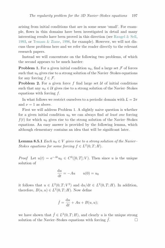
The regularity problem for the 3D Navier–Stokes equations 197
arising from initial conditions that are in some sense ‘small’. For exam-ple, flows in thin domains have been investigated in detail and manyinteresting results have been proved in this direction (see Raugel & Sell,1993, or Temam & Ziane, 1996, for example). However, we will not dis-cuss these problems here and we refer the reader directly to the relevantresearch papers.
Instead we will concentrate on the following two problems, of whichthe second appears to be much harder:
Problem 1. For a given initial condition u0, find a large set F of forcessuch that u0 gives rise to a strong solution of the Navier–Stokes equationsfor any forcing f ∈ F .Problem 2. For a given force f find large set U of initial conditionssuch that any u0 ∈ U gives rise to a strong solution of the Navier–Stokesequations with forcing f .
In what follows we restrict ourselves to a periodic domain with L = 2πand ν = 1 as above.
First we will address Problem 1. A slightly naive question is whetherfor a given initial condition u0 we can always find at least one forcingf(t) for which u0 gives rise to the strong solution of the Navier–Stokesequations. An easy answer is provided by the following lemma, whichalthough elementary contains an idea that will be significant later.
Lemma 8.5.1 Each u0 ∈ V gives rise to a strong solution of the Navier–Stokes equations for some forcing f ∈ L2(0, T ;H).
Proof Let u(t) = e−Atu0 ∈ C0([0, T ];V ). Then since u is the uniquesolution of
dudt
= −Au u(0) = u0
it follows that u ∈ L2(0, T ;V 2) and du/dt ∈ L2(0, T ;H). In addition,therefore, B(u, u) ∈ L2(0, T ;H). Now define
f =dudt
+Au+B(u, u);
we have shown that f ∈ L2(0, T ;H), and clearly u is the unique strongsolution of the Navier–Stokes equations with forcing f .
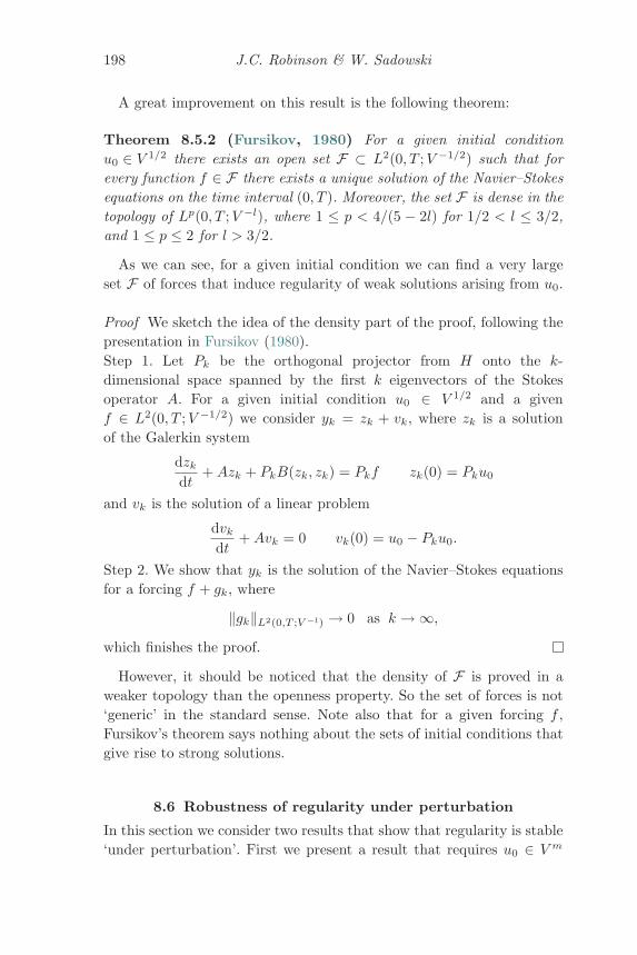
198 J.C. Robinson & W. Sadowski
A great improvement on this result is the following theorem:
Theorem 8.5.2 (Fursikov, 1980) For a given initial conditionu0 ∈ V 1/2 there exists an open set F ⊂ L2(0, T ;V −1/2) such that forevery function f ∈ F there exists a unique solution of the Navier–Stokesequations on the time interval (0, T ). Moreover, the set F is dense in thetopology of Lp(0, T ;V −l), where 1 ≤ p < 4/(5 − 2l) for 1/2 < l ≤ 3/2,and 1 ≤ p ≤ 2 for l > 3/2.
As we can see, for a given initial condition we can find a very largeset F of forces that induce regularity of weak solutions arising from u0.
Proof We sketch the idea of the density part of the proof, following thepresentation in Fursikov (1980).Step 1. Let Pk be the orthogonal projector from H onto the k-dimensional space spanned by the first k eigenvectors of the Stokesoperator A. For a given initial condition u0 ∈ V 1/2 and a givenf ∈ L2(0, T ;V −1/2) we consider yk = zk + vk, where zk is a solutionof the Galerkin system
dzk
dt+Azk + PkB(zk, zk) = Pkf zk(0) = Pku0
and vk is the solution of a linear problem
dvk
dt+Avk = 0 vk(0) = u0 − Pku0.
Step 2. We show that yk is the solution of the Navier–Stokes equationsfor a forcing f + gk, where
‖gk‖L2(0,T ;V −l) → 0 as k → ∞,
which finishes the proof.
However, it should be noticed that the density of F is proved in aweaker topology than the openness property. So the set of forces is not‘generic’ in the standard sense. Note also that for a given forcing f ,Fursikov’s theorem says nothing about the sets of initial conditions thatgive rise to strong solutions.
8.6 Robustness of regularity under perturbation
In this section we consider two results that show that regularity is stable‘under perturbation’. First we present a result that requires u0 ∈ V m
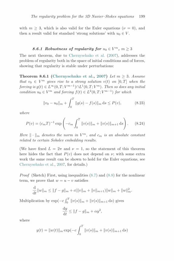
The regularity problem for the 3D Navier–Stokes equations 199
with m ≥ 3, which is also valid for the Euler equations (ν = 0), andthen a result valid for standard ‘strong solutions’ with u0 ∈ V .
8.6.1 Robustness of regularity for u0 ∈ V m, m ≥ 3
The next theorem, due to Chernysehnko et al. (2007), addresses theproblem of regularity both in the space of initial conditions and of forces,showing that regularity is stable under perturbations:
Theorem 8.6.1 (Chernysehnko et al., 2007) Let m ≥ 3. Assumethat v0 ∈ V m gives rise to a strong solution v(t) on [0, T ] when theforcing is g(t) ∈ L∞(0, T ;V m−1)∩L1(0, T ;V m). Then so does any initialcondition u0 ∈ V m and forcing f(t) ∈ L2(0, T ;V m−1) for which
‖v0 − u0‖m +∫ T
0
‖g(s) − f(s)‖m ds ≤ P (v), (8.23)
where
P (v) = (cmT )−1 exp
(−cm
∫ T
0
‖v(s)‖m + ‖v(s)‖m+1 ds
). (8.24)
Here ‖ · ‖m denotes the norm in V m, and cm is an absolute constantrelated to certain Sobolev embedding results.
(We have fixed L = 2π and ν = 1, so the statement of this theoremhere hides the fact that P (v) does not depend on ν; with some extrawork the same result can be shown to hold for the Euler equations, seeChernysehnko et al., 2007, for details.)
Proof (Sketch) First, using inequalities (8.7) and (8.8) for the nonlinearterm, we prove that w = u− v satisfies
ddt
‖w‖m ≤ ‖f − g‖m + c(‖v‖m + ‖v‖m+1)‖w‖m + ‖w‖2m.
Multiplication by exp(−c ∫ T
0‖v(s)‖m + ‖v(s)‖m+1 ds) gives
dydt
≤ ‖f − g‖m + αy2,
where
y(t) = ‖w(t)‖m exp(−c∫ T
0
‖v(s)‖m + ‖v(s)‖m+1 ds)
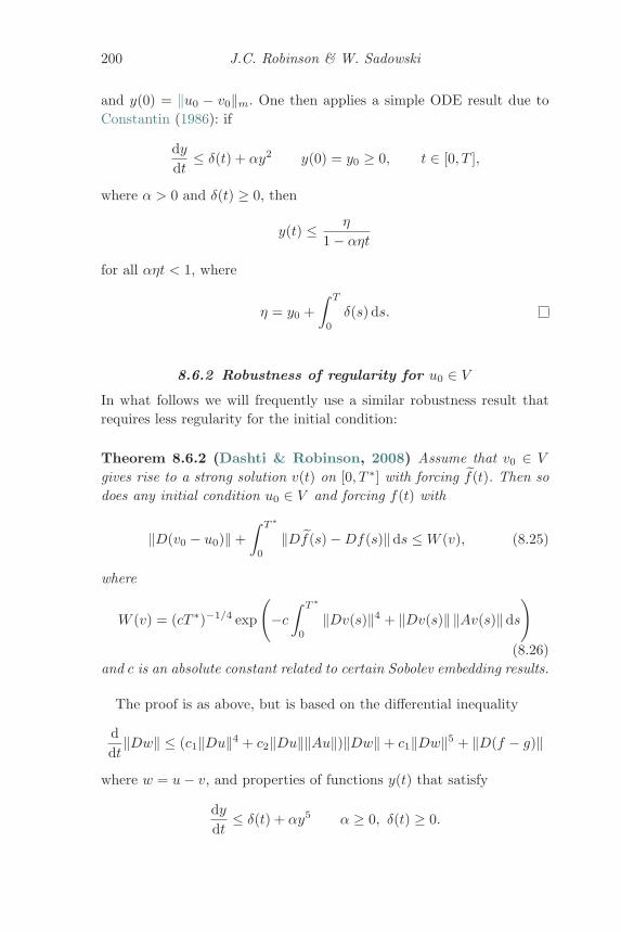
200 J.C. Robinson & W. Sadowski
and y(0) = ‖u0 − v0‖m. One then applies a simple ODE result due toConstantin (1986): if
dydt
≤ δ(t) + αy2 y(0) = y0 ≥ 0, t ∈ [0, T ],
where α > 0 and δ(t) ≥ 0, then
y(t) ≤ η
1 − αηt
for all αηt < 1, where
η = y0 +∫ T
0
δ(s) ds.
8.6.2 Robustness of regularity for u0 ∈ V
In what follows we will frequently use a similar robustness result thatrequires less regularity for the initial condition:
Theorem 8.6.2 (Dashti & Robinson, 2008) Assume that v0 ∈ V
gives rise to a strong solution v(t) on [0, T ∗] with forcing f(t). Then sodoes any initial condition u0 ∈ V and forcing f(t) with
‖D(v0 − u0)‖ +∫ T∗
0
‖Df(s) −Df(s)‖ds ≤W (v), (8.25)
where
W (v) = (cT ∗)−1/4 exp
(−c
∫ T∗
0
‖Dv(s)‖4 + ‖Dv(s)‖ ‖Av(s)‖ds
)(8.26)
and c is an absolute constant related to certain Sobolev embedding results.
The proof is as above, but is based on the differential inequality
ddt
‖Dw‖ ≤ (c1‖Du‖4 + c2‖Du‖‖Au‖)‖Dw‖ + c1‖Dw‖5 + ‖D(f − g)‖
where w = u− v, and properties of functions y(t) that satisfy
dydt
≤ δ(t) + αy5 α ≥ 0, δ(t) ≥ 0.
The regularity problem for the 3D Navier–Stokes equations 201
8.7 Numerical verification of regularity
We now discuss how this robustness result can be used to provide amethod of (at least theoretical) numerical verification of regularity: firstfor a single initial condition, then for any bounded set in V 2, and finallyfor any bounded set in V .
8.7.1 Verification for a single initial condition in V
The following result is a simple consequence of Theorem 8.6.2 whenit is combined with the idea used in Lemma 8.5.1 that if both v andf := dv/dt + Av + B(v, v) are sufficiently regular then v is the uniquestrong solution of the Navier–Stokes equation du/dt+Au+B(u, u) = f .
Corollary 8.7.1 (Dashti & Robinson, 2008) Suppose that thefunction v ∈ L∞(0, T ;V ) ∩ L2(0, T ;V 2) satisfies
dvdt
+Av +B(v, v) ∈ L1(0, T ;V ) ∩ L2(0, T ;V )
and
‖Dv(0) −Du0‖ +∫ T
0
∥∥∥∥dvdt
(s) +Av(s) +B(v(s), v(s))∥∥∥∥
1
ds ≤W (v),
(8.27)where W (v) is defined by (8.26). Then u is a regular solution of theNavier–Stokes equations with u ∈ L∞(0, T ;V ) ∩ L2(0, T ;V 2).
This corollary tells us that we can obtain a purely theoretical result(regularity of the solution arising from a given initial condition) fromapproximate numerical computations. (Of course, a numerical solutionwill be given only at discrete time points but this is not an obstacle sinceone can, for example, construct u via linear interpolation between thesepoints.)
In fact, it is possible to verify regularity corresponding to a particularinitial condition u0 in a finite time: if u0 does give rise to a regularsolution on [0, T ], finite-dimensional Galerkin approximations (based onthe eigenfunctions of the Stokes operator) can be guaranteed to convergeto u(t) (see Dashti & Robinson, 2008, for details). It follows that ifu0 leads to such a regular solution, one can take v to be the result ofsuccessively larger-dimensional Galerkin approximations until (8.27) issatisfied. On the other hand, if a weak solution arising from u0 evolvesto produce a singularity then the numerical computation will not be
202 J.C. Robinson & W. Sadowski
able to show this. In other words, we can verify regularity of a strongsolution, but we cannot obtain in this way any proof of the hypotheticalbreakdown of regularity of a weak solution.
8.7.2 Verification for a ball in V 2
Since it is possible to use numerical computations to check regularityof a single given initial condition it is sensible to ask whether numericalcomputations may improve the theoretical result given in Theorem 8.3.4.The answer is yes. However, before we prove this we will investigate anauxiliary problem. Instead of considering a set of initial conditions inthe space V we will, for the moment, restrict our attention to a set ofmore regular initial conditions that is a ball in V 2. Our aim is to presenta method of verifying the following statement, for some fixed S > 0:
Statement 1. Every initial condition with ‖Au0‖ ≤ S gives rise to a strongsolution that exists for all t ≥ 0.
Following Robinson & Sadowski (2008) we will sketch the proof of thefollowing theorem.
Theorem 8.7.2 (Robinson & Sadowski, 2008) Assume that State-ment 1 is true. Then it is possible to verify it numerically in a finitetime.
Proof (Sketch)Step 1. We have already remarked (Theorem 8.3.5) that any weak solu-tion is strong for t ≥ T ∗∗, where T ∗∗ depends only on the norm ofthe initial data in V . So we need only verify regularity on the boundedinterval [0, T ∗∗].Step 2. We assume that Statement 1 is true. Following Constantin, Foias,& Temam (1985) one can prove, under this assumption, that for anyT > 0 there exist constants DS(T ) and ES(T ) such that every initialcondition u0 with ‖Au0‖ ≤ S gives rise to a solution u satisfying
sup0≤t≤T
‖Du(s)‖ ≤ DS and∫ T
0
‖Au(s)‖2 ds ≤ ES .
Step 3. Using these bounds one can deduce that for any such a solutionu the following integral is uniformly bounded:∫ T∗∗
0
‖Du(s)‖4 + ‖Du(s)‖ ‖Au(s)‖ds < Q.
The regularity problem for the 3D Navier–Stokes equations 203
It follows that there exists a δ = δ(S) such that if ‖Au0‖ ≤ S thenW (u) > δ. Theorem 8.6.2 implies that every initial condition v0 ∈ V
with
‖Du0 −Dv0‖ < δ
also gives rise to a strong solution on [0, T ∗∗].Step 4. One can find an explicit finite collection of balls in V of radiusδ that cover the ball in V 2 (centred at the origin) of radius S. One canthen check numerically, using Corollary 8.7.1, that the centres of eachof these balls are initial conditions giving rise to strong solutions on[0, T ∗∗].
Observe that the proof is based only on an assumption of regularityof solutions arising from initial conditions with ‖Au0‖ ≤ S. Whether ornot singularities may occur in solutions arising from initial conditions u0
with ‖Au0‖ > S has no effect on the possibility of numerical verificationof regularity of solutions with ‖Au0‖ < S.
8.7.3 Verification for a ball in V
Our main aim now is to show that we can verify numerically the regu-larity of solutions arising from initial conditions in some ball in V . Moreprecisely, we wish to verify the following statement for some fixed R > 0:
Statement 2. Every initial condition with ‖Du0‖ ≤ R gives rise to a strongsolution that exists for all t ≥ 0.
In order to verify this we have to make the stronger assumption thatthe Navier–Stokes equations are in fact regular, i.e. that Statement 2holds for any value of R > 0.
Theorem 8.7.3 (Robinson & Sadowski, 2008) Assume that theNavier–Stokes equations are regular. Then it is possible to verify State-ment 2 numerically in a finite time.
Proof (Sketch)Step 1. We find time TR > 0 such that every solution with initial con-dition ‖Du0‖ ≤ R is regular on the interval [0, TR] and has an explicitbound on ‖Au(TR)‖. We can do this using a result due to Foias & Temam(1989) on the Gevrey regularity of solutions, a consequence of which is
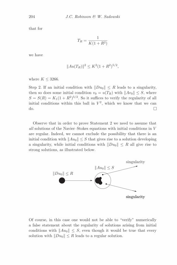
204 J.C. Robinson & W. Sadowski
that for
TR =1
K(1 +R2)
we have
‖Au(TR)‖2 ≤ K2(1 +R2)5/2,
where K ≤ 3266.
Step 2. If an initial condition with ‖Du0‖ ≤ R leads to a singularity,then so does some initial condition v0 = u(TR) with ‖Av0‖ ≤ S, whereS = S(R) = K1(1 + R2)5/2. So it suffices to verify the regularity of allinitial conditions within this ball in V 2, which we know that we cando.
Observe that in order to prove Statement 2 we need to assume thatall solutions of the Navier–Stokes equations with initial conditions in Vare regular. Indeed, we cannot exclude the possibility that there is aninitial condition with ‖Au0‖ ≤ S that gives rise to a solution developinga singularity, while initial conditions with ‖Du0‖ ≤ R all give rise tostrong solutions, as illustrated below.
���������������
����������
� � ��‖Au0‖ ≤ S
‖Du0‖ ≤ R
singularity
singularity
singularity
Of course, in this case one would not be able to “verify” numericallya false statement about the regularity of solutions arising from initialconditions with ‖Au0‖ ≤ S, even though it would be true that everysolution with ‖Du0‖ ≤ R leads to a regular solution.
The regularity problem for the 3D Navier–Stokes equations 205
8.8 Acknowledgements
JCR was partially supported by a Royal Society University ResearchFellowship and the Leverhulme Trust; WS was partially supported byPolish Government Grant 1 P03A 017 30.
References
Beale, J.T., Kato, T., & Majda, A.J. (1984) Remarks on the breakdown ofsmooth solutions for the 3-D Euler equations. Comm. Math. Phys. 94,61–66.
Berselli, L.C. & Galdi, G.P. (2002) Regularity criterion involving the pressurefor the weak solutions to the Navier–Stokes equations. Proc. Amer. Math.Soc. 130, 3585–3595.
Caffarelli, L., Kohn, R., & Nirenberg, L. (1982) Partial regularity of suitableweak solutions of the Navier–Stokes equations. Comm. Pure Appl. Math.35, 771–831.
Chae, D. & Choe, H.J. (1999) Regularity of solutions to the Navier–Stokesequation. Electronic Journal of Differential Equations 5, 1–7.
Chae, D. & Lee, J. (2001) Regularity criterion in terms of pressure for theNavier–Stokes equations. Nonlinear Anal. 46, 727–735.
Chernysehnko, S.I., Constantin, P., Robinson, J.C., & Titi, E.S. (2007) A pos-teriori regularity of the three-dimensional Navier–Stokes equations fromnumerical computations. J. Math. Phys. 48, 1–15.
Cheskidov, A., Friedlander, S., & Shvydkoy, R. (2008) On the energy equal-ity for weak solutions of the 3D Navier–Stokes equations, submitted.arXiv:0704.2089.
Constantin, P. (1986) Note on loss of regularity for solutions of the 3Dincompressible Euler and related equations. Comm. Math. Phys. 104,311–326
Constantin, P. & Foias, C. (1988) Navier–Stokes Equations. University ofChicago Press, Chicago.
Constantin, P., Foias, C., & Temam, R. (1985) Attractors representing turbu-lent flows. Memoirs of the Amer. Math. Soc. 53 (314), Providence, RhodeIsland.
Dashti, M. & Robinson, J.C. (2008) An a posteriori condition on the numeri-cal approximations of the Navier–Stokes equations for the existence of astrong solution. SIAM J. Numer. Anal. 46, 3136–3150.
Doering, C.R. & Gibbon, J.D. (1995) Applied Analysis of the Navier–Stokes Equations. Cambridge Texts in Applied Mathematics, CambridgeUniversity Press, Cambridge.
Escauriaza, L., Seregin, G.A., & Sverak, V. (2003) L3,∞-solutions of Navier–Stokes equations and backward uniqueness. Russian Math. Surveys 58,211–250.
Fabes, E., Jones, B., & Riviere, N. (1972) The initial value problem for theNavier–Stokes equations with data in Lp. Arch. Rat. Mech. Anal. 45,222–248.
Falconer, K. (1990) Fractal Geometry. Wiley, Chichester.
206 J.C. Robinson & W. Sadowski
Fefferman, C.L. (2000) Existence and smoothness of the Navier–Stokes equa-tion. http://www.claymath.org/millennium/Navier-Stokes Equations/navierstokes.pdf.
Foias, C. & Temam, R. (1989) Gevrey class of regularity for the solutions ofthe Navier–Stokes equations. J. Funct. Anal. 87, 359–369.
Fursikov, A.V. (1980) On some control problems and results concerning theunique solvability of a mixed boundary value problem for the threedimensional Navier–Stokes and Euler systems. Soviet Math. Dokl. 21,181–188.
Hopf, E. (1951) Uber die Anfangswertaufgabe fur die hydrodynamischenGrundgleichungen. Math. Nachr. 4, 213–231.
Leray, J. (1934) Essai sur le mouvement d’un fluide visqueux emplissantl’espace. Acta Math. 63, 193–248.
Raugel, G. & Sell, G.R. (1993) Navier–Stokes equations on thin 3D domains. I:global attractors and global regularity of solutions. Journal of the Amer.Math. Soc. 6, 503–568.
Robinson, J.C. (2001) Infinite-dimensional dynamical systems. CambridgeTexts in Applied Mathematics, Cambridge University Press, Cambridge.
Robinson, J.C. (2006) Regularity and singularity in the three-dimensionalNavier–Stokes equations. Boletın de la Sociedad Espanola de MatematicaAplicada 35, 43–71.
Robinson, J.C. & Sadowski, W. (2007) Decay of weak solutions and the sin-gular set of the three-dimensional Navier–Stokes equations. Nonlinearity20, 1185–1191.
Robinson, J.C. & Sadowski, W. (2008) Numerical verification of regularity inthe three-dimensional Navier–Stokes equations for bounded sets of initialdata. Asymptot. Anal. 59, 39–50.
Scheffer, V. (1976) Turbulence and Hausdorff dimension, in Turbulenceand Navier–Stokes equations, Orsay 1975, Springer LNM 565, 174–183,Springer-Verlag, Berlin.
Serrin, J. (1962) On the interior regularity of weak solutions of the Navier–Stokes equations. Arch. Rat. Mech. Anal. 9, 187–191.
Temam, R. (2001) Navier–Stokes Equations. North Holland, Amsterdam,1977. Reprinted by AMS Chelsea.
Temam, R. & Ziane, M. (1996) Navier–Stokes equations in three-dimensionalthin domains with various boundary conditions. Adv. in DifferentialEquations 1, 499–546.
da Veiga, H.B. (1995) Concerning the regularity problem for the solutions ofthe Navier–Stokes equations. C. R. Acad. Sci. Paris I 321, 405–408.
Zhou, Y. (2006) On the regularity criteria in terms of pressure of the Navier–Stokes equations in R3. Proc. Amer. Math. Soc. 134, 149–156.
9
Contour dynamics for the surfacequasi-geostrophic equation
Jose L. RodrigoMathematics Institute, University of Warwick,
Coventry, CV4 7AL. [email protected]
Abstract
We review recent progress on the evolution of sharp fronts for the surfacequasi-geostrophic equations and related problems, with special emphasison techniques that can be extended to the study of vortex dynamics forthe 3D Euler equations.
9.1 Introduction
In these notes we will review a series of problems related to contourdynamics for two-dimensional active-scalar equations. More precisely,the central problem we will concentrate on is the evolution of sharp frontsfor the surface quasi-geostrophic equation, obtained by considering theevolution of initial data given by the indicator of a smooth, open set bythe equations
Dθ
Dt:=
∂θ
∂t+ u · ∇θ = 0, (9.1)
u = ∇⊥ψ = (−∂x2ψ, ∂x1ψ), (9.2)
(−Δ)12ψ = θ. (9.3)
Here the variable θ represents a two-dimensional active scalar (potentialtemperature in physical terms) advected by the velocity field u and ψ isthe stream function. Finally, we define the fractional Laplacian in termsof the Fourier transform,
(−Δ)12ψ(ξ) = |ξ|ψ(ξ).
We will refer to the system (9.1)–(9.3) as SQG.The term ‘sharp front’, to denote the boundary of the set whose indi-
cator we are considering, stems from the fact that the SQG system was
Published in Partial Differential Equations and Fluid Mechanics, edited byJames C. Robinson and Jose L. Rodrigo. c© Cambridge University Press 2009.
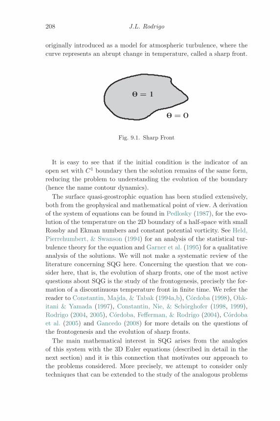
208 J.L. Rodrigo
originally introduced as a model for atmospheric turbulence, where thecurve represents an abrupt change in temperature, called a sharp front.
θ = 0
θ = 1
Fig. 9.1. Sharp Front
It is easy to see that if the initial condition is the indicator of anopen set with C1 boundary then the solution remains of the same form,reducing the problem to understanding the evolution of the boundary(hence the name contour dynamics).
The surface quasi-geostrophic equation has been studied extensively,both from the geophysical and mathematical point of view. A derivationof the system of equations can be found in Pedlosky (1987), for the evo-lution of the temperature on the 2D boundary of a half-space with smallRossby and Ekman numbers and constant potential vorticity. See Held,Pierrehumbert, & Swanson (1994) for an analysis of the statistical tur-bulence theory for the equation and Garner et al. (1995) for a qualitativeanalysis of the solutions. We will not make a systematic review of theliterature concerning SQG here. Concerning the question that we con-sider here, that is, the evolution of sharp fronts, one of the most activequestions about SQG is the study of the frontogenesis, precisely the for-mation of a discontinuous temperature front in finite time. We refer thereader to Constantin, Majda, & Tabak (1994a,b), Cordoba (1998), Ohk-itani & Yamada (1997), Constantin, Nie, & Schorghofer (1998, 1999),Rodrigo (2004, 2005), Cordoba, Fefferman, & Rodrigo (2004), Cordobaet al. (2005) and Gancedo (2008) for more details on the questions ofthe frontogenesis and the evolution of sharp fronts.
The main mathematical interest in SQG arises from the analogiesof this system with the 3D Euler equations (described in detail in thenext section) and it is this connection that motivates our approach tothe problems considered. More precisely, we attempt to consider onlytechniques that can be extended to the study of the analogous problems
Contour dynamics for SQG 209
in 3D Euler, that is, as we will see in next section, the study of vortexlines for 3D Euler.
9.2 SQG and 3D Euler
As mentioned before, the main mathematical interest in the surfacequasi-geostrophic system lies in its strong analogies with the 3D Eulerequation. SQG presents a two-dimensional equation that contains manyof the features of 3D Euler. We will present a very brief review of theanalogies between these two equations. These similarities are best estab-lished when considering 3D Euler in vorticity form. Recall that in termsof the vorticity ω = curlu, 3D Euler becomes
Dω
Dt= (∇u)ω,
where u = (u1, u2, u3) is the 3D velocity satisfying div u = 0.In particular, we observe that by differentiating equation (9.1) we
obtainD(∇⊥θ)Dt
= (∇u)∇⊥θ.
This shows a very strong analogy between the 3D Euler equationand QG, where ∇⊥θ plays the role of ω. We briefly recall some furtheranalogies:
• The velocity is recovered via the formulas
u(x) =∫
R3K3(y)ω(x+ y)dy u(x) =
∫R2K2(y)∇⊥θ(x+ y)dy,
where the kernels Kd, d = 2, 3 are homogeneous of degree 1 − d.Additionally, the strain matrix (the symmetric part of the gradient ofthe velocity) can be recovered via a singular integral operator, givenby kernels of degree −d.
• Both systems have conserved energy.• Both |ω| and |∇⊥θ| evolve according to the same type of equation.
(|ω| measures the infinitesimal length of a vortex line).• Both systems have analogous conditions for a break up of a solution,
that is, the well-known criterion due to Beale, Kato, & Majda (1984)translates directly to SQG with ∇⊥θ in place of ω.
• The integral curves of ω, and of ∇⊥θ move with the fluid.
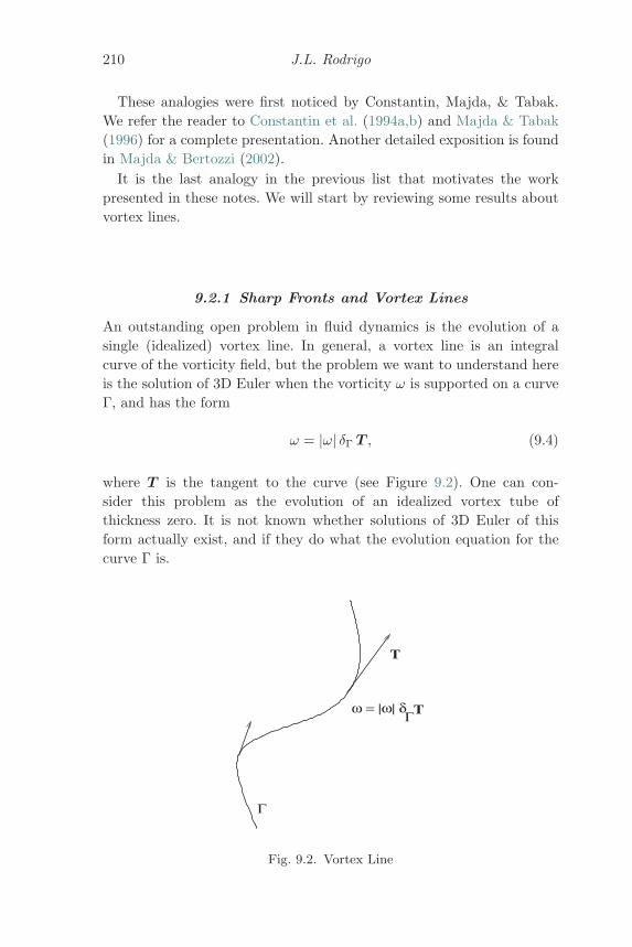
210 J.L. Rodrigo
These analogies were first noticed by Constantin, Majda, & Tabak.We refer the reader to Constantin et al. (1994a,b) and Majda & Tabak(1996) for a complete presentation. Another detailed exposition is foundin Majda & Bertozzi (2002).
It is the last analogy in the previous list that motivates the workpresented in these notes. We will start by reviewing some results aboutvortex lines.
9.2.1 Sharp Fronts and Vortex Lines
An outstanding open problem in fluid dynamics is the evolution of asingle (idealized) vortex line. In general, a vortex line is an integralcurve of the vorticity field, but the problem we want to understand hereis the solution of 3D Euler when the vorticity ω is supported on a curveΓ, and has the form
ω = |ω| δΓ T , (9.4)
where T is the tangent to the curve (see Figure 9.2). One can con-sider this problem as the evolution of an idealized vortex tube ofthickness zero. It is not known whether solutions of 3D Euler of thisform actually exist, and if they do what the evolution equation for thecurve Γ is.
TΓ
Γ
ω = |ω| δ
T
Fig. 9.2. Vortex Line
Contour dynamics for SQG 211
The main difficulty in the study the evolution of a vortex line is thatwe need to understand the velocity field (given by the Biot–Savart Law)
u(x, t) =1
4π
∫x− y
|x− y|3 × ω(y, t) dy, (9.5)
which appears in the Euler equation in vorticity form
Dω
Dt= (∇u)ω.
Equation (9.5) is obtained by inverting the curl operator under rea-sonable assumptions on the regularity and decay of ω that, of course, arenot satisfied by a vortex line as defined in (9.4). In the case of a vortexline, the velocity is of order
u(x) ≈ 1distance to the curve
,
which means that u is not in L2(R3). This means that we cannot useany of the various definitions of solution for 3D Euler to understand avortex line.
No rigorous derivation of an equation for the evolution of a vortex lineis known but a well-known approximation for its evolution is given bythe equation
∂tγ = κB, (9.6)
where κ is the curvature of γ and B is the binormal. Equation (9.6) isknown as the LIA equation (Locally Induced Approximation), and wasfirst introduced by da Rios in 1906. We refer the reader to Ricca (1996)for an excellent review of the work of da Rios and the derivation of theLIA equation.
Equation (9.6) can be converted into a nonlinear Schrodinger equationusing the Hasimoto transformation. Using this formulation the existenceof self-similar singular solutions has been proved (Vega, 2003; Gutierrez,Rivas, & Vega, 2003; Gutierrez & Vega, 2004). We also remark thatmodifications of equation (9.6) have been studied for example by Klein& Majda (1991a,b). The main reason for introducing these modifiedequations is to obtain an equation that contains self-stretching, sincethe length of any curve evolving under (9.6) remains constant in time.
Postponing the details until the next section, we compare in the pic-ture below the velocity fields for both problems, to show that sharpfronts for SQG retain many of the features of vortex lines, while being amore tractable problem. In particular, the velocity field for SQG whilestill singular, contains only a logarithmic singularity (see Figure 9.3).
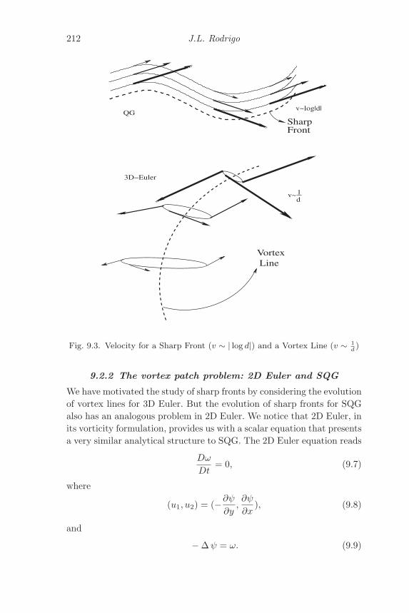
212 J.L. Rodrigo
VortexLine
SharpFront
QG
3D−Euler
v~1d
v~log|d|
Fig. 9.3. Velocity for a Sharp Front (v ∼ | log d|) and a Vortex Line (v ∼ 1d)
9.2.2 The vortex patch problem: 2D Euler and SQG
We have motivated the study of sharp fronts by considering the evolutionof vortex lines for 3D Euler. But the evolution of sharp fronts for SQGalso has an analogous problem in 2D Euler. We notice that 2D Euler, inits vorticity formulation, provides us with a scalar equation that presentsa very similar analytical structure to SQG. The 2D Euler equation reads
Dω
Dt= 0, (9.7)
where
(u1, u2) = (−∂ψ∂y
,∂ψ
∂x), (9.8)
and
− Δψ = ω. (9.9)
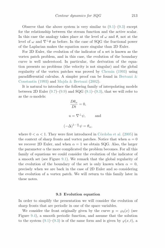
Contour dynamics for SQG 213
Observe that the above system is very similar to (9.1)–(9.3) exceptfor the relationship between the stream function and the active scalar.In this case the analogy takes place at the level of ω and θ, not at thelevel of ω and ∇⊥θ as before. In the case of SQG the fractional powerof the Laplacian makes the equation more singular than 2D Euler.
For 2D Euler, the evolution of the indicator of a set is known as thevortex patch problem, and in this case, the evolution of the boundarycurve is well understood. In particular, the derivation of the equa-tion presents no problems (the velocity is not singular) and the globalregularity of the vortex patches was proved by Chemin (1993) usingparadifferential calculus. A simpler proof can be found in Bertozzi &Constantin (1993) and Majda & Bertozzi (2002).
It is natural to introduce the following family of interpolating modelsbetween 2D Euler (9.7)–(9.9) and SQG (9.1)–(9.3), that we will refer toas the α-models:
Dθα
Dt= 0,
u = ∇⊥ψ, and
(−Δ)1−α2 ψ = θα,
where 0 < α < 1. They were first introduced in Cordoba et al. (2005) inthe context of sharp fronts and vortex patches. Notice that when α = 0we recover 2D Euler, and when α = 1 we obtain SQG. Also, the largerthe parameter α the more complicated the problem becomes. For all thisfamily of equations we could consider the evolution of the indicator ofa smooth set (see Figure 9.1). We remark that the global regularity ofthe evolution of the boundary of the set is only known when α = 0,precisely when we are back in the case of 2D Euler and so consideringthe evolution of a vortex patch. We will return to this family later inthese notes.
9.3 Evolution equation
In order to simplify the presentation we will consider the evolution ofsharp fronts that are periodic in one of the space variables.
We consider the front originally given by the curve y = ϕ0(x) (seeFigure 9.4), a smooth periodic function, and assume that the solutionto the system (9.1)–(9.3) is of the same form and is given by ϕ(x, t), a
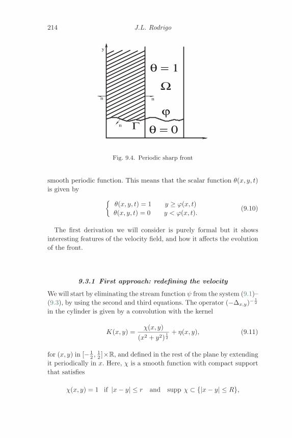
214 J.L. Rodrigo
θ = 1
nn
n
y
θ = 0
Ω
Γϕ
Fig. 9.4. Periodic sharp front
smooth periodic function. This means that the scalar function θ(x, y, t)is given by {
θ(x, y, t) = 1 y ≥ ϕ(x, t)θ(x, y, t) = 0 y < ϕ(x, t).
(9.10)
The first derivation we will consider is purely formal but it showsinteresting features of the velocity field, and how it affects the evolutionof the front.
9.3.1 First approach: redefining the velocity
We will start by eliminating the stream function ψ from the system (9.1)–(9.3), by using the second and third equations. The operator (−Δx,y)−
12
in the cylinder is given by a convolution with the kernel
K(x, y) =χ(x, y)
(x2 + y2)12
+ η(x, y), (9.11)
for (x, y) in [−12 ,
12 ]×R, and defined in the rest of the plane by extending
it periodically in x. Here, χ is a smooth function with compact supportthat satisfies
χ(x, y) = 1 if |x− y| ≤ r and supp χ ⊂ {|x− y| ≤ R},
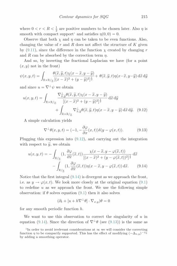
Contour dynamics for SQG 215
where 0 < r < R < 12 are positive numbers to be chosen later. Also η is
smooth with compact support1 and satisfies η(0, 0) = 0.Observe that both χ and η can be taken to be even functions. Also,
changing the value of r and R does not affect the structure of K givenby (9.11), since the difference in the function χ created by changing r
and R can be absorbed by the correction term η.And so, by inverting the fractional Laplacian we have (for a point
(x, y) not in the front)
ψ(x, y, t) =∫
R×R/Z
θ(x, y, t)χ(x− x, y − y)[(x− x)2 + (y − y)2]
12
+ θ(x, y, t)η(x−x, y−y) dx dy
and since u = ∇⊥ψ we obtain
u(x, y, t) =∫
R×R/Z
∇⊥x,yθ(x, y, t)χ(x− x, y − y)
[(x− x)2 + (y − y)2]12
dxdy
+∫
R×R/Z
∇⊥x,yθ(x, y, t)η(x− x, y − y) dx dy. (9.12)
A simple calculation yields
∇⊥θ(x, y, t) = (−1,−∂ϕ∂x
(x, t))δ(y − ϕ(x, t)). (9.13)
Plugging this expression into (9.12), and carrying out the integrationwith respect to y, we obtain
u(x, y, t) = −∫
R/Z
(1,∂ϕ
∂x(x, t))
χ(x− x, y − ϕ(x, t))[(x− x)2 + (y − ϕ(x, t))2]
12
dx
−∫
R/Z
(1,∂ϕ
∂x(x, t))η(x− x, y − ϕ(x, t)) dx. (9.14)
Notice that the first integral (9.14) is divergent as we approach the front,i.e. as y → ϕ(x, t). We look more closely at the original equation (9.1)to redefine u as we approach the front. We use the following simpleobservation: if θ solves equation (9.1) then it also solves
(∂t + [u+ h∇⊥θ] · ∇x,y)θ = 0
for any smooth periodic function h.
We want to use this observation to correct the singularity of u inequation (9.14). Since the direction of ∇⊥θ (see (9.13)) is the same as
1In order to avoid irrelevant considerations at ∞ we will consider the correctingfunction η to be compactly supported. This has the effect of modifying (−Δx,y)−1/2
by adding a smoothing operator.
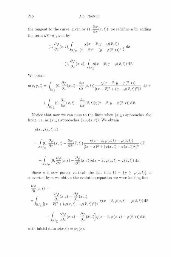
216 J.L. Rodrigo
the tangent to the curve, given by (1,∂ϕ
∂x(x, t)), we redefine u by adding
the term h∇⊥θ given by
(1,∂ϕ
∂x(x, t))
∫R/
Z
χ(x− x, y − ϕ(x, t))[(x− x)2 + (y − ϕ(x, t))2]
12
dx
+(1,∂ϕ
∂x(x, t))
∫R/
Z
η(x− x, y − ϕ(x, t)) dx.
We obtain
u(x, y, t) =∫
R/Z
(0,∂ϕ
∂x(x, t)−∂ϕ
∂x(x, t))
χ(x− x, y − ϕ(x, t))[(x− x)2 + (y − ϕ(x, t))2]
12
dx +
+∫
R/Z
(0,∂ϕ
∂x(x, t) − ∂ϕ
∂x(x, t))η(x− x, y − ϕ(x, t)) dx.
Notice that now we can pass to the limit when (x, y) approaches thefront, i.e. as (x, y) approaches (x, ϕ(x, t)). We obtain
u(x, ϕ(x, t), t) =
=∫
R/Z
(0,∂ϕ
∂x(x, t) − ∂ϕ
∂x(x, t))
χ(x− x, ϕ(x, t) − ϕ(x, t))[(x− x)2 + (ϕ(x, t) − ϕ(x, t))2]
12
dx
+∫
R/Z
(0,∂ϕ
∂x(x, t) − ∂ϕ
∂x(x, t))η(x− x, ϕ(x, t) − ϕ(x, t)) dx.
Since u is now purely vertical, the fact that Ω = {y ≥ ϕ(x, t)} isconvected by u we obtain the evolution equation we were looking for:
∂ϕ
∂t(x, t) =
=∫
R/Z
∂ϕ
∂x(x, t) − ∂ϕ
∂x(x, t)
[(x− x)2 + (ϕ(x, t) − ϕ(x, t))2]12χ(x− x, ϕ(x, t) − ϕ(x, t)) dx
+∫
R/Z
[∂ϕ∂x
(x, t) − ∂ϕ
∂x(x, t)
]η(x− x, ϕ(x, t) − ϕ(x, t)) dx,
with initial data ϕ(x, 0) = ϕ0(x).
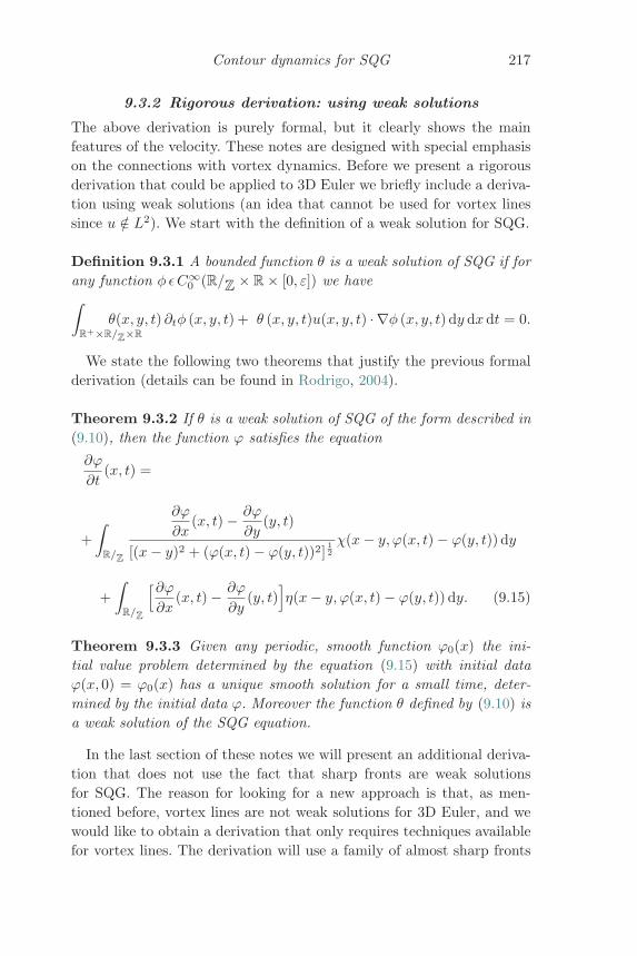
Contour dynamics for SQG 217
9.3.2 Rigorous derivation: using weak solutions
The above derivation is purely formal, but it clearly shows the mainfeatures of the velocity. These notes are designed with special emphasison the connections with vortex dynamics. Before we present a rigorousderivation that could be applied to 3D Euler we briefly include a deriva-tion using weak solutions (an idea that cannot be used for vortex linessince u /∈ L2). We start with the definition of a weak solution for SQG.
Definition 9.3.1 A bounded function θ is a weak solution of SQG if forany function φ εC∞
0 (R/Z × R × [0, ε]) we have∫R+×R/
Z×R
θ(x, y, t) ∂tφ (x, y, t) + θ (x, y, t)u(x, y, t) · ∇φ (x, y, t) dy dxdt = 0.
We state the following two theorems that justify the previous formalderivation (details can be found in Rodrigo, 2004).
Theorem 9.3.2 If θ is a weak solution of SQG of the form described in(9.10), then the function ϕ satisfies the equation
∂ϕ
∂t(x, t) =
+∫
R/Z
∂ϕ
∂x(x, t) − ∂ϕ
∂y(y, t)
[(x− y)2 + (ϕ(x, t) − ϕ(y, t))2]12χ(x− y, ϕ(x, t) − ϕ(y, t)) dy
+∫
R/Z
[∂ϕ∂x
(x, t) − ∂ϕ
∂y(y, t)
]η(x− y, ϕ(x, t) − ϕ(y, t)) dy. (9.15)
Theorem 9.3.3 Given any periodic, smooth function ϕ0(x) the ini-tial value problem determined by the equation (9.15) with initial dataϕ(x, 0) = ϕ0(x) has a unique smooth solution for a small time, deter-mined by the initial data ϕ. Moreover the function θ defined by (9.10) isa weak solution of the SQG equation.
In the last section of these notes we will present an additional deriva-tion that does not use the fact that sharp fronts are weak solutionsfor SQG. The reason for looking for a new approach is that, as men-tioned before, vortex lines are not weak solutions for 3D Euler, and wewould like to obtain a derivation that only requires techniques availablefor vortex lines. The derivation will use a family of almost sharp fronts
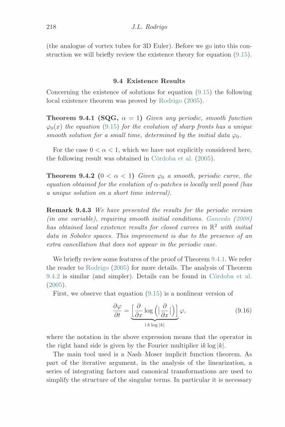
218 J.L. Rodrigo
(the analogue of vortex tubes for 3D Euler). Before we go into this con-struction we will briefly review the existence theory for equation (9.15).
9.4 Existence Results
Concerning the existence of solutions for equation (9.15) the followinglocal existence theorem was proved by Rodrigo (2005).
Theorem 9.4.1 (SQG, α = 1) Given any periodic, smooth functionϕ0(x) the equation (9.15) for the evolution of sharp fronts has a uniquesmooth solution for a small time, determined by the initial data ϕ0.
For the case 0 < α < 1, which we have not explicitly considered here,the following result was obtained in Cordoba et al. (2005).
Theorem 9.4.2 (0 < α < 1) Given ϕ0 a smooth, periodic curve, theequation obtained for the evolution of α-patches is locally well posed (hasa unique solution on a short time interval).
Remark 9.4.3 We have presented the results for the periodic version(in one variable), requiring smooth initial conditions. Gancedo (2008)has obtained local existence results for closed curves in R2 with initialdata in Sobolev spaces. This improvement is due to the presence of anextra cancellation that does not appear in the periodic case.
We briefly review some features of the proof of Theorem 9.4.1. We referthe reader to Rodrigo (2005) for more details. The analysis of Theorem9.4.2 is similar (and simpler). Details can be found in Cordoba et al.(2005).
First, we observe that equation (9.15) is a nonlinear version of
∂ϕ
∂t=[ ∂∂x
log(∣∣ ∂∂x
∣∣)]︸ ︷︷ ︸i k log |k|
ϕ, (9.16)
where the notation in the above expression means that the operator inthe right hand side is given by the Fourier multiplier ik log |k|.
The main tool used is a Nash–Moser implicit function theorem. Aspart of the iterative argument, in the analysis of the linearization, aseries of integrating factors and canonical transformations are used tosimplify the structure of the singular terms. In particular it is necessary
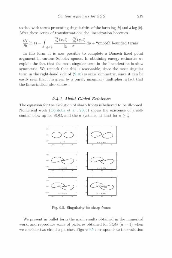
Contour dynamics for SQG 219
to deal with terms presenting singularities of the form log |k| and k log |k|.After these series of transformations the linearization becomes
∂f
∂t(x, t) =
∫|y|< 1
2
∂f∂x (x, t) − ∂f
∂y (y, t)
|y − x| dy + “smooth bounded terms”
In this form, it is now possible to complete a Banach fixed pointargument in various Sobolev spaces. In obtaining energy estimates weexploit the fact that the most singular term in the linearization is skewsymmetric. We remark that this is reasonable, since the most singularterm in the right-hand side of (9.16) is skew symmetric, since it can beeasily seen that it is given by a purely imaginary multiplier, a fact thatthe linearization also shares.
9.4.1 About Global Existence
The equation for the evolution of sharp fronts is believed to be ill-posed.Numerical work (Cordoba et al., 2005) shows the existence of a self-similar blow up for SQG, and the α systems, at least for α ≥ 1
2 .
−2 0 2
−2
0
2
t = 0
−2 0 2
−2
0
2
t = 1.962
−2 0 2
−2
0
2
t = 3.300
−2 0 2
−2
0
2
t = 4.031
−2 0 2
−2
0
2
t = 4.369
−2 0 2
−2
0
2
t = 4.464
Fig. 9.5. Singularity for sharp fronts
We present in bullet form the main results obtained in the numericalwork, and reproduce some of pictures obtained for SQG (α = 1) whenwe consider two circular patches. Figure 9.5 corresponds to the evolution
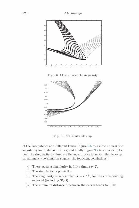
220 J.L. Rodrigo
−0.1 0 0.1 0.2 0.3 0.4 0.5 0.6 0.7 0.8 0.9
−0.2
−0.1
0
0.1
0.2
0.3
0.4
0.5
Fig. 9.6. Close up near the singularity
−0.25 −0.2 −0.15 −0.1 −0.05 0 0.05 0.1 0.15 0.2 0.25
−0.25
−0.2
−0.15
−0.1
−0.05
0
0.05
0.1
0.15
0.2
0.25
Fig. 9.7. Self-similar blow up
of the two patches at 6 different times, Figure 9.6 to a close up near thesingularity for 10 different times, and finally Figure 9.7 to a rescaled plotnear the singularity to illustrate the asymptotically self-similar blow-up.In summary, the numerics suggest the following conclusions:
(i) There exists a singularity in finite time, say T .(ii) The singularity is point-like.
(iii) The singularity is self-similar (T − t)−1α , for the corresponding
α-model (including SQG).(iv) The minimum distance d between the curves tends to 0 like
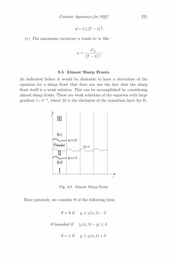
Contour dynamics for SQG 221
d ∼ C1(T − t)1α .
(v) The maximum curvature κ tends to ∞ like
κ ∼ C2
(T − t)1α
.
9.5 Almost Sharp Fronts
As indicated before it would be desirable to have a derivation of theequation for a sharp front that does not use the fact that the sharpfront itself is a weak solution. This can be accomplished by consideringalmost sharp fronts. These are weak solutions of the equation with largegradient (∼ δ−1, where 2δ is the thickness of the transition layer for θ).
ΙΙΙ
Ι
ΙΙ
x
y
θ=1
ϕ −δ(x,t)
ϕ (x,t)
θ=0
θ bounded
ϕ +δ(x,t)
Fig. 9.8. Almost Sharp Front
More precisely, we consider θ of the following form
θ = 0 if y ≤ ϕ(x, t) − δ
θ bounded if |ϕ(x, t) − y| ≤ δ
θ = 1 if y ≥ ϕ(x, t) + δ
222 J.L. Rodrigo
where ϕ is a smooth periodic function and 0 < δ < 12 . We will denote the
three regions determining the structure of θ by I, II and III respectively(see Figure 9.8).
This type of solution can be thought of as the analogue of a vortextube for 3D Euler, i.e. a regularized vortex line.
9.5.1 Stability and derivation
Almost-sharp fronts can be used to obtain a derivation of equation (9.15)using the following theorem (see Cordoba et al., 2004).
Theorem 9.5.1 If θ is an almost-sharp front and is a weak solution ofSQG, then ϕ satisfies the equation
∂ϕ
∂t(x, t) =
=∫
R/Z
∂ϕ
∂x(x, t) − ∂ϕ
∂x(x, t)
[(x− x)2 + (ϕ(x, t) − ϕ(x, t))2]12χ(x− x, ϕ(x, t) − ϕ(x, t)) dx
+∫
R/Z
[∂ϕ∂x
(x, t) − ∂ϕ
∂x(x, t)
]η(x− x, ϕ(x, t) − ϕ(x, t)) dx
+ Error,
with |Error| ≤ C δ| log δ| where C depends only on ‖θ‖L∞ and ‖∇ϕ‖L∞ .
Remark 9.5.2 Note that an almost-sharp front specifies the functionϕ up to an error of order δ. The above theorem provides an evolutionequation for the function ϕ up to an error of order δ| log δ|.
Proof We briefly sketch the main ideas in the proof. Recall the definitionof a weak solution∫
R+×R/Z×R
θ(x, y, t) ∂tφ (x, y, t) + θ (x, y, t)u(x, y, t) · ∇φ (x, y, t) dy dx dt = 0.
We need to study the above equation in the three regions of θ. Noticethat region I does not contribute since θ = 0. We will concentrate on
Contour dynamics for SQG 223
region II, where θ is simply bounded. There we have∫II×R+
θ(x, y, t)∂tφ(x, y, t) dxdy dt = O(δ)
since θ = O(1), and area(II) = O(δ).
We still have to estimate∫
R2u · (1IIθ∇φ) dxdy. Recall that the velocity
for SQG is given by
u = ∇⊥((−Δ)−12 θ) = K ∗ θ,
where K looks locally like the orthogonal of the Riesz transform.
In order to complete the estimate all that is required are two classicalresults in harmonic analysis. Namely, the fact that the Riesz transformmaps bounded functions into functions of exponential class and the factthat the integral of a function of exponential class on a domain of areaδ is of order δ log δ. The first guarantees the fact that u is of exponentialclass, and hence the whole integrand in the expression below, while thesecond directly leads to
∫R2u · (1IIθ∇φ) dxdy = O(δ log δ).
Region III can be handled in a similar manner to obtain more errorterms of order δ log δ and the terms from the equation of a sharp frontin a similar manner to Theorem 9.3.2.
9.5.2 Construction of Almost-Sharp Fronts
In order to use Theorem 9.5.1 to find a derivation of the equation, weneed to prove the existence of almost-sharp fronts of thickness δ for somesmall time independent of δ. Notice that only local existence results areknow for SQG and so the time of existence for a family of almost-sharpfronts is not uniform with respect to δ, but rather goes to zero as δgoes to zero. In this section we present some of the ideas involved inthe constructions of some families of solutions such that for δ ≤ δ0 thesolutions θδ exist for at least time T , independent of δ. In particularwe concentrate on the crucial problem of finding a limit equation whenδ goes to zero. This corresponds to upcoming joint work with CharlesFefferman.
224 J.L. Rodrigo
As a first approach, we look for solutions of the form
θδ(x, y, t) = Ω(x,y − ϕ(x, t)
δ, t),
where Ω is smooth and satisfies⎧⎨⎩Ω(x, ξ, t) = 1
2 ξ > 1Ω(x, ξ, t) smooth |ξ| ≤ 1
Ω(x, ξ, t) = −12 ξ < −1.
(9.17)
In order to simplify the presentation, we will use the followingexpression for the velocity
u(x, y, t) =∫
(−∂yθ(x, y, t), ∂xθ(x, y, t))[(x− x)2 + (y − y)2]
12
dxdy,
which amounts to taking the cut-off function χ as 1 and the correctionterm η as 0, as can be seen by comparing the above formula with thetrue expression for u (see (9.12).
Once the equation is rewritten in terms of Ω, x, ξ we expect, since thelogarithmic singularity in the velocity for a sharp front does not affectthe shape of the front, to obtain an equation of the form
1δ
(Sharp Front Equation for ϕ) + terms of order 1 depending on Ω, x, ξ
so that if the curve ϕ solves the sharp front equation we could take alimit in the equation. Unfortunately that is not the case, and while wedo obtain the term of order 1
δ there are a priori harmless terms for whichwe cannot take a limit. Namely, among the terms arising from u ·∇θ wehave the term∫ ∫ Ωξ(x, ξ, t)Ωx(x, ξ, t) − Ωx(x, ξ, t)Ωξ(x, ξ, t)
[(x− x)2 + (ϕ(x, t) − ϕ(x, t) + δ(ξ − ξ))2]12
dxdξ.
The problem with this term is that when δ = 0 the kernel looses thedependence on ξ making the integral singular! We have∫ ∫ Ωξ(x, ξ, t)Ωx(x, ξ, t) − Ωx(x, ξ, t)Ωξ(x, ξ, t)
[(x− x)2 + (ϕ(x, t) − ϕ(x, t))2]12
dxdξ =
=∫
Ωx(x, ξ, t) − ∫Ωx(x, ξ, t)dξ Ωξ(x, ξ, t)
[(x− x)2 + (ϕ(x, t) − ϕ(x, t))2]12
dx
since∫
Ωξ(x, ξ, t) dξ = 1 due to the form of Ω (see (9.17)).
Contour dynamics for SQG 225
At this formal level, having made δ = 0 we observe that an integrationof the equation with respect to ξ makes the singular term convergent∫ ∫
Ωx(x, ξ, t) dξ − ∫Ωx(x, ξ, t) dξ
[(x− x)2 + (ϕ(x, t) − ϕ(x, t))2]12
dx.
Remark 9.5.3The above formal calculation suggests that
(i)∫
Ω(x, ξ, t) dξ =: h(x, t) satisfies a much better equation.(ii) If the velocity can be expressed in terms of h rather than in terms
of Ω, then we can convert the initial equation into a transport-likeequation with coefficients that tend to ∞ as δ → 0.
The main reason for the presence of these unexpected singular termscan be found in the expression for the velocity. We know that it is sin-gular and of order log δ and we have seen in the initial derivation of theequation that it does not influence the evolution of the curve, but thereis a nonsingular term, which will lead to a singularity in the term u ·∇θ.We have, for δ > 0, an expression of the form
u(x, ξ, t) ≈ log δ (1, ϕ(x, t)) + δ log δ term + · · ·or more precisely
u(x, t) = (log δ)α(x, t)(1, ϕ(x, t))
− δ log δ{αx(x, t)ξ + αx(x, t)h(x, t) + α(x, t)hx(x, t)
}(0, 1) + · · · ,
where α only depends on ϕ and h(x, t) =∫
Ω(x, ξ, t) dξ. Observe thatas remarked before, the velocity can be expressed in terms of h(x, t).
Notice that since the gradient of θ is of order δ−1, the term of orderδ log δ will generate a singularity. In more detail, we have
∇θ = Ωx(x, ξ, t)(1, 0) + (−ϕ(x, t), 1)1δ
Ωξ(x, ξ, t)
and so
u · ∇θ = log δ{αΩx − [
αx ξ + αxh+ αhx
]Ωξ
}+ · · ·
Notice that integrating in the vertical direction, that is with respectto ξ, has the same regularizing effect, since a simple calculation showsthat ∫
αΩx − [αx ξ + αxh+ αhx
]Ωξ dξ = 0.
226 J.L. Rodrigo
The advantage of integrating the equation with respect to ξ is that itallows us to obtain a “simple” equation for h(x, t) =
∫Ω(x, ξ, t)dξ, that
actually has a limit as δ goes to 0.We use its solution in the original equation for Ω,
Ωt + log δ{αΩx − [
αx ξ + αxh+ αhx
]Ωξ
}+ · · · = 0, (9.18)
which is now a transport-like equation since h is known.While equation (9.18) does not have a limiting form when δ goes to
zero, all we need to do is integrate the following vector fields⎧⎪⎪⎪⎨⎪⎪⎪⎩dxdt
= α(x, t)
dξdt
= −[αx ξ + αxh+ αhx],
with initial conditions x(0) = x0 and ξ(0) = ξ0.The process of integrating the system of ODEs and rewriting the equa-
tion in terms of x0 and ξ0 corresponds to unwinding the logarithmicdivergence that appears in u · ∇θ, before considering the map
(x, y, t) �−→ (x,y − ϕ(x, t)
δ, t).
It is this unwinding process that makes it possible to obtain a limitingequation for Ω, in terms of the Lagrangian coordinates x0 and ξ0.
Acknowledgements
The author was partially supported by MTM2005–05980, Ministeriode Educacion y Ciencia (Spain) and MTM2008–03754, Ministerio deCiencia e Innovacion (Spain). The author wishes to acknowledge A.M.Mancho for producing Figures 9.5, 9.6, and 9.7.
ReferencesBeale, J.T., Kato, T., & Majda, A.J. (1984) Remarks on the breakdown of
smooth solutions for the 3-D Euler equations. Comm. Math. Phys. 94,61–66.
Bertozzi, A.L. & Constantin, P. (1993) Global regularity for vortex patches.Comm. Math. Phys. 152, no. 1, 19–28.
Chemin, J.Y. (1993) Persistance de structures geometriques dans les fluidesincompressibles bidimensionnels. Ann. Ec. Norm. Super. 26, no. 4, 1–16.
Constantin, P., Majda, A., & Tabak, E. (1994a) Singular front formation in amodel for quasigesotrophic flow. Phys. Fluids 6, no. 1, 9–11.
Constantin, P., Majda, A., & Tabak, E. (1994b) Formation of strong fronts inthe 2−D quasigeostrophic thermal active scalar. Nonlinearity 7, no. 6,1495–1533.
Contour dynamics for SQG 227
Constantin, P., Nie, Q., & Schorghofer, N. (1998) Nonsingular surface quasi-geostrophic flow. Phys. Lett. A 241, no. 3, 168–172.
Constantin, P., Nie, Q., & Schorghofer, N. (1999) Front formation in an activescalar equation. Phys. Rev. E (3) 60, no. 3, 2858–2863.
Cordoba, D. (1998) Nonexistence of simple hyperbolic blow-up for the quasi-geostrophic equation. Ann. of Math. (2) 148, no. 3, 1135–1152.
Cordoba, D., Fefferman, C., & Rodrigo, J.L. (2004) Almost sharp fronts forthe surface Quasi-Geostrophic equation. Proc. Natl. Acad. Sci. USA 101,no. 9, 2487–2491.
Cordoba, D., Fontelos, M.A., Mancho, A.M., & Rodrigo, J.L. (2005) Evidenceof singularities for a family of contour dynamics equations. Proc. Natl.Acad. Sci. USA 102, no. 17, 5949–5952.
da Rios, L.S. (1906) Sul moto d’un liquido indefinito con un filetto vorticosodi forma qualunque. Rend. Circ. Mat. Palermo 22, 117–135.
Gancedo, F. (2008) Existence for the α-patch model and the QG sharp frontin Sobolev spaces. Adv. Math. 217, no. 6, 2569–2598.
Garner, S.T., Held, I.M., Pierrehumbert, R.T., & Swanson, K. (1995) Surfacequasi-geostrophic dynamics. J. Fluid Mech. 282, 1–20.
Gutierrez, S. & Vega, L. (2004) Self-similar solutions of the localized inductionapproximation: singularity formation. Nonlinearity 17, no. 6, 2091–2136.
Gutierrez, S., Rivas, J., & Vega, L. (2003) Formation of singularities andself-similar vortex motion under the localized induction approximation.Comm. Partial Differential Equations 28, no. 5-6, 927–968.
Held, I.M., Pierrehumbert, R.T., & Swanson. K. (1994) Spectra of local andnonlocal two dimensional turbulence. Chaos, Solitons and Fractals 4,1111–1116.
Klein, R. & Majda, A.J. (1991a) Self-stretching of a perturbed vortex filament.I. The asymptotic equation for deviations from a straight line. Phys. D49, no. 3, 323–352.
Klein, R. & Majda, A.J. (1991b) Self-stretching of perturbed vortex filaments.II. Structure of solutions. Phys. D 53, no. 2-4, 267–294.
Majda, A.J. & Bertozzi, A. (2002) Vorticity and incompressible flow. Cam-bridge Texts in applied Mathematics, 27.
Madja, A.J. & Tabak, E. (1996) A two-dimensional model for quasigeostrophicflow: comparison with the two-dimensional Euler flow. Physica D 98, no.2-4, 515–522.
Ohkitani, K. & Yamada, M. (1997) Inviscid and inviscid-limit behavior of asurface quasigeostrophic flow. Phys. Fluids 9, no. 4, 876–882.
Pedlosky, J. (1987) Geophysical Fluid Dynamics. Springer-Verlag, 345–368and 653–670, New York.
Ricca, R.L. (1996) The contributions of da Rios and Levi-Civita to asymptoticpotential theory and vortex filament dynamics. Fluid Dynam. Res. 18, no.5, 245–268.
Rodrigo, J.L. (2004) The vortex patch problem for the Quasi-Geostrophicequation. PNAS 101, no. 9, 2484–2486.
Rodrigo, J.L. (2005) On the evolution of sharp fronts for the quasi-geostrophicequation. Comm. Pure Appl. Math. 58, no. 6, 821–866.
Vega, L. (2003) Kink solutions of the binormal flow. Journees Equations auxDerivees Partielles, XIV, Univ. Nantes, Nantes.
10
Theory and applications of statisticalsolutions of the Navier–Stokes equations
Ricardo M.S. RosaInstituto de Matematica,
Universidade Federal do Rio de Janeiro,Caixa Postal 68530 Ilha do Fundao, Rio de Janeiro,
RJ 21945-970. [email protected]
Abstract
Since the 1970s the use of statistical solutions of the Navier–Stokes equa-tions has led to a number of rigorous results for turbulent flows. Thispaper reviews the concept of a statistical solution, its role in the math-ematical foundation of the theory of turbulence, some of its successes,and the theoretical and applied challenges that still remain. The theoryis illustrated in detail for the particular case of a two-dimensional flowdriven by a uniform pressure gradient.
10.1 Introduction
It is believed that turbulent fluid motions are well modelled by theNavier–Stokes equations. However, due to the complicated nature ofthese equations, most of our understanding of turbulence relies to a greatextent on laboratory experiments and on heuristic and phenomenologicalarguments. Nevertheless, a number of rigorous mathematical results havebeen obtained directly from the Navier–Stokes equations, particularly inthe last two decades.
Of great interest in turbulence theory are mean quantities, which arein general well behaved, in contrast to the corresponding instantaneousvalues, which tend to vary quite dramatically in time. The treatment ofmean values, however, is a delicate problem, as remarked by Monin &Yaglom (1975). In practice time and space averages are the most gener-ally used, while in theory averages with respect to a large ensemble offlows avoid some analytical difficulties and have a more universal char-acter. In the conventional theory of turbulence, all three types of averageare taken to agree by invoking some sort of ergodic property, althoughno general result in this direction exists.
Published in Partial Differential Equations and Fluid Mechanics, edited byJames C. Robinson and Jose L. Rodrigo. c© Cambridge University Press 2009.
Statistical solutions of the Navier–Stokes equations 229
Rigorous results for time and space averages can be obtained fromindividual weak solutions of the Navier–Stokes equations, while rigorousresults for ensemble averages are obtained via the concept of statisticalsolutions.
Probability theory has been used to formalize the concept of an ensem-ble average since very early in the development of the conventionaltheory. Later on, Hopf (1952) published one of the first works witha more mathematical flavour. A rigorous mathematical foundation forthis formalization, however, came only with the introduction of statis-tical solutions by Foias (1972, 1973). Another rigorous framework wasintroduced a few years later by Vishik & Fursikov (1977, 1988). Bothframeworks involve measures on function spaces and require a numberof deep results in analysis. Just as for individual solutions of the Navier–Stokes equations, there are various challenging problems regarding theregularity of such statistical solutions.
Statistical solutions can be time-dependent or stationary in time. Thetime-dependent case is suitable, for instance, for the study of decayingturbulence, while the stationary case applies to turbulence in statisticalequilibrium in time.
The stationary statistical solution is a generalization of the notionof an invariant measure for a semigroup. The major difficulty here liesin the fact that the three-dimensional Navier–Stokes equations are notknow to generate a well-defined semigroup. An invariant measure inthis case does not make sense, and the statistical solution allows one toaddress this issue. In the two-dimensional case, in which the associatedsemigroup is well defined, both notions coincide.
Beyond the theoretical issues permeating the concept of statisticalsolutions, a number of applications have been given yielding rigorousbounds for characteristic physical quantities taken in the mean withrespect to such solutions. Estimates have been obtained involving themean energy dissipation rate, mean enstrophy dissipation rate, meanskin-drag coefficient, mean kinetic-energy flux between different scalesof motions, and so on. A number of such rigorous results are related toimportant properties of turbulent flows as derived in the conventionaltheory of turbulence via heuristic or phenomenological arguments, andyield rigorous results such as estimates for the number of degrees offreedom, estimates related to the Kolmogorov energy dissipation law,exponential decay of the power spectrum in the two-dimensional case,conditions for the existence of an energy cascade in the three-dimensional
230 R. Rosa
case, conditions for the existence of inverse energy and direct enstrophycascades in the two-dimensional case, etc.
While the results for time averages and ensemble averages haverecently paralleled one another, our main concern in this article is onensemble averages. We recall the definition of a statistical solution, dis-cuss some of the associated delicate theoretical problems, and mention,without proof, a number of rigorous estimates obtained recently. Wealso include, for the sake of illustration, a proof of two estimates per-taining to a two-dimensional channel flow driven by a uniform pressuregradient. More precisely, we prove the curious fact that, for this geom-etry, the plane Poiseuille flow minimizes the mean rate of enstrophydissipation and maximizes the mean rate of energy dissipation. Theseminimization and maximization properties are with respect to invariantmeasures of the semigroup generated by the two-dimensional Navier–Stokes equations; a Dirac measure concentrated on the velocity field forthe Poiseuille flow is one such measure. The minimization part is newwhile the maximization is an adaptation of a corresponding recent resultfor the three-dimensional channel problem treated by Ramos, Rosa, &Temam (2008). Although this example is for a two-dimensional prob-lem, it has many similarities with the corresponding estimates for thethree-dimensional problem and so serves as a useful illustration.
10.2 The incompressible Navier–Stokes equations
We consider the incompressible Navier–Stokes equations (NSE) andwrite them in the form
∂u∂t
− νΔu + (u · ∇)u + ∇p = f , ∇ · u = 0, (10.1)
where u = u(x, t) = (u1, u2, u3) denotes the three-component velocityfield, x = (x1, x2, x3) is the space variable; t is the time variable; νis the kinematic viscosity; p = p(x, t) is the kinematic pressure; andf = f(x, t) = (f1, f2, f3) is the density of volume forces.
For the classical mathematical theory of the NSE the reader is referredto Ladyzhenskaya (1963), Temam (1984), and Constantin & Foias(1988), which are based on the earlier works of Leray (1933, 1934a,b)and Hopf (1951).
The spatial domain is denoted by Ω ⊂ R3. The boundary condi-tions are assumed to be homogeneous and may be no-slip, periodic,or combinations of these, as in the case of a periodic channel flow. In
Statistical solutions of the Navier–Stokes equations 231
the fully-periodic case, the velocity field and the forcing term can beassumed, without loss of generality, to have zero space average over theperiodic domain, while in cases involving no-slip boundary conditions,the domain is assumed to be either bounded or to have finite width inone direction. In all these cases, the Stokes operator (the linear part ofthe time-independent problem), which will be denoted by A, is strictlypositive.
The NSE can be written in the formdudt
= F(u),
in a suitable space H of square-integrable divergence-free vector fieldswith the appropriate boundary conditions, and with an appropriatefunction F : V → V ′, with V ⊆ H ⊆ V ′. Here, V is the space ofdivergence-free vector fields that are square integrable along with theirfirst order partial derivatives, equipped with the appropriate boundaryconditions, and V ′ is its dual. See, for instance, Section 6 for a precisedefinition of these spaces in the case of a two-dimensional channel. Thepressure can, in principle, be determined from the vector field u.
The L2-like norm and inner product in H are denoted by | · | and (·, ·),while the H1
0 -like norm and inner product in V are denoted by ‖ · ‖ and((·, ·)). For the sake of simplicity, the duality product between V and V ′
is also denoted by (·, ·). These inner products can be written explicitlyas
(u,v) =∫
Ω
3∑i=1
uivi dx and ((u,v)) =∫
Ω
3∑i,j=1
∂ui
∂xj
∂vi
∂xjdx.
The inner products and duality are such that (Au,v) = ((u,v)) for allu,v ∈ V . Under the assumptions made on the domain Ω, there is alargest positive number λ1 > 0 such that (Au,u) = ‖u‖2 ≥ λ1|u|2, forall u ∈ V .
The nonlinear term gives rise to a bilinear form B : V × V → V ′,which can be defined by duality through
(B(u,v),w) = b(u,v,w),
where the trilinear term b : V × V × V → R is defined by
b(u,v,w) =∫
Ω
((u · ∇)v) · w dx. (10.2)
In the three-dimensional case and with typical boundary conditions(periodic, no-slip, etc.) it is well-known that given an initial velocity field
232 R. Rosa
u0 in H, there exists a weak solution (in a suitable sense) u = u(t) thatis defined for all t ≥ 0 and satisfies u(0) = u0. In fact, there exists aweak solution satisfying, in addition, a certain energy-type inequality,and this solution is called a Leray–Hopf weak solution. But the regu-larity obtained for this solution is still not sufficient to guarantee itsuniqueness. If the initial condition is more regular, however, there existsa time interval, 0 ≤ t < δ, with δ depending on the size of the ini-tial condition in an appropriate sense, in which the solution is regularand unique. Therefore, we have local unique regular solutions and globalLeray–Hopf weak solutions.
In the two-dimensional case, the system is more amenable to anal-ysis, and the existence and uniqueness of global regular solutions areknown for arbitrary initial conditions in H; the system is well-posed andgenerates a continuous nonlinear semigroup {S(t)}t≥0 in H.
10.3 Mean quantities and statistical solutions
As mentioned in the introduction, there is much interest in mean quanti-ties, whether space averaged, time averaged, or with respect to ensembleaverages. One is typically interested in relating different quantities inthe hope of finding universal properties of turbulent flows (Kolmogorov,1941; Batchelor, 1953; Monin & Yaglom, 1975; Hinze, 1975; Tennekes &Lumley, 1972; Lesieur, 1997; Frisch, 1995; Foias et al., 2001a; Rosa, 2002,2006).
Types of averages
Time averages can be easily defined for a given individual solutionu(t) of the NSE through the relation
1T
∫ t+T
t
ϕ(u(s)) ds,
where T > 0 and ϕ : H → R is associated with some physical quantityone wants to consider (energy, rate of energy dissipation, etc.). Spaceaverages can be defined in a similar way, although one must be carefulwith the boundary conditions.
In situations where a statistical equilibrium is of interest (the instan-taneous quantities still vary widely in time but average quantities seemstationary), an “infinite-time” average is often more meaningful and inthis case the limit as T → ∞ is taken in the definition of the average.One may assume that the limit exists, although there is no general result
Statistical solutions of the Navier–Stokes equations 233
about this, or one may consider superior or inferior limits, or generalizedlimits.
In the case of ensemble averages, one may think of a number of exper-iments yielding velocity fields u(n)(t), t ≥ 0, n = 1, . . . , N , and take theaverage over this ensemble of experiments:
1N
N∑n=1
ϕ(u(n)(t)).
In a more general and rigorous way, one considers a family of probabilitymeasures {μt}t≥0 defined on H, representing the probability distributionof the velocity field, and takes the average∫
H
ϕ(v) dμt(v).
Note that in this expression the quantity v is simply a dummy variablein the integration. The important quantity is the family of measures.
Time-dependent statistical solutions
In relation with the ensemble averages, for a family {μt}t≥0 of mea-sures to be meaningful for the flow, it must satisfy an equation analogousto the Liouville equation in Statistical Mechanics, namely
ddt
∫H
Φ(v) dμt(v) =∫
H
(F(v),Φ′(v)) dμt(v), (10.3)
for all “test” functions Φ. Note that since F : V → V ′, the measuresμt are expected to be carried by V , while the derivative Φ′(v) of thetest function is assumed to belong to V . More general test functionsϕ : H → R can be evaluated in the mean, but for the Liouville equation,a more restricted set of test functions Φ is considered, which explainsthe difference in notation.
The reason behind the form of the equation (10.3) can be seen fromthe following derivation, for a family of measures
μt =1N
N∑i=1
δu(n)(t)
234 R. Rosa
obtained as a convex combination of Dirac measures concentrated on Nweak solutions u(n)(t) with equal probability 1/N :
ddt
∫H
Φ(v) dμt(v) =ddt
1N
N∑n=1
Φ(u(n)(t)) =1N
N∑n=1
ddt
Φ(u(n)(t))
=1N
N∑n=1
Φ′(u(n)(t)) ◦ ddt
u(n)(t) =1N
N∑n=1
Φ′(u(n)(t)) ◦ F(u(n)(t))
=1N
N∑n=1
(F(u(n)(t)),Φ′(u(n))) =∫
H
(F(v),Φ′(v)) dμt(v).
Other conditions are necessary for the problem to make sense. Forinstance, concerning generalized moments, one asks that
t �→∫
H
ϕ(v) dμt(v) is measurable on [0,∞), (10.4)
for every bounded and continuous real-valued function ϕ on H.From the physical point of view, it is also natural to assume that the
mean kinetic energy per unit mass and the mean rate of enstrophy dissi-pation per unit time per unit mass are finite, at least almost everywhere.In fact, it is assumed that
t �→∫
H
|v|2 dμt(v) ∈ L∞loc(0,∞), t �→
∫H
‖v‖2 dμt(v) ∈ L2loc(0,∞),
(10.5)as obtained for individual weak solutions.
Finally, a mean energy inequality for the statistical solutions isalso assumed, analogous to the energy inequality for Leray–Hopf weaksolutions:
12
∫H
|v|2 dμt(v) + ν
∫ t
t′
∫H
‖v‖2 dμs(v) ds
≤ 12
∫H
|v|2 dμt′(v) +∫ t
t′
∫H
(f ,v) dμs(v) ds,
for almost all t′ ≥ 0, and all t ≥ t′, with t′ = 0 included.A stricter definition requires the validity of the following strengthened
form of energy inequality:
12
∫H
ψ(|v|2) dμt(v) + ν
∫ t
t′
∫H
ψ′ (|v|2) ‖v‖2 dμs(v) ds
≤ 12
∫H
ψ(|v|2) dμt′(v) +
∫ t
t′
∫H
ψ′ (|v|2) (f ,v) dμs(v) ds, (10.6)
Statistical solutions of the Navier–Stokes equations 235
for almost all t′ ≥ 0, and all t ≥ t′, with t′ = 0 included, and forarbitrary non-negative, non-decreasing, continuously-differentiable real-valued function ψ with bounded derivative.
For us here, a family {μt}t≥0 of Borel probability measures on H
satisfying (10.4), (10.5), (10.3) (for suitable “test functions”), and thestrengthened energy inequality (10.6), is then called a statistical solutionon the time-interval [0,∞).
This fundamental definition of statistical solution, which makes rigor-ous the concept of ensemble average which is ubiquitous in turbulencetheory, was introduced by Foias (1972, 1973) (see also Hopf, 1952;Vishik & Fursikov, 1977, 1988; Foias et al., 2001a) and has beenextensively exploited in recent years.
As with the theory for individual solutions, there are results on theglobal existence of statistical solutions. The typical assumption on theinitial measure μ0 is that it has finite mean kinetic energy:∫
H
|v|2 dμ0(v) <∞.
Stationary statistical solutions
In the case of turbulence in statistical equilibrium in time, the meanquantities are time independent and a single measure μ represents thestatistics of the flow. This measure satisfies the stationary Liouville-typeequation, ∫
H
(F(v),Φ′(v)) dμ(v) = 0, (10.7)
and is called a stationary statistical solution of the NSE.These stationary statistical solutions, first defined by Foias (1973),
are generalizations of invariant measures, which do not make sense inthe three-dimensional case due to the lack of a global well-posednessresult. Foias’s concept of a statistical solution was inspired by the twounpublished pioneering works of Prodi (1960, 1961), who insisted on theidea of working with measures that should be invariant in some suitablesense.
In the two-dimensional case, on the other hand, global well-posednesshas been established and ensemble averages can be interpreted as aver-ages with respect to invariant measures. We recall here that an invariantBorel probability measure for the semigroup {S(t)}t≥0 generated by the2D Navier–Stokes equations is a Borel probability measure μ on H such
236 R. Rosa
that
μ(S(t)−1E) = μ(E),
for all Borel sets E in H. An analogous definition of a stationary sta-tistical solution can be given in 2D and it turns out to be equivalent tothe definition of an invariant measure (Foias, 1973; Foias et al., 2001a).
Time-average stationary statistical solutions
A particular class of stationary statistical solution is obtained via ageneralized limit of time averages of weak solutions, as in the Krylov–Bogoliubov procedure (Krylov & Bogoliubov, 1937). More precisely,given a global weak solution u = u(t) defined for all t ≥ 0 and given afunction ϕ : H → R which is weakly continuous on H, the generalizedBanach limit
ϕ �→ LimT→∞
1T
∫ T
0
ϕ(u(t)) dt
exists and defines a linear functional with respect to ϕ. It can be proved(Bercovici et al., 1995; Foias et al., 2001a) that there exists a measureμu associated with this weak solution for which
LimT→∞
1T
∫ T
0
ϕ(u(t)) dt =∫
H
ϕ(v) dμu(v)
for all such ϕ, and that this measure is a stationary statistical solution.
Mean quantities
A common notation for the ensemble average is 〈·〉. We use thisnotation here in the case of stationary statistical turbulence, writing
〈ϕ〉 =∫
H
ϕ(u) dμ(u),
for a given functional ϕ : H → R and a given stationary statisticalsolution μ on H. The quantity 〈ϕ〉 is called a generalized moment.
Taking κ0 to denote a macro-scale wavenumber (e.g. κ0 = λ1/21 ), two
important examples of ensemble-averaged mean quantities in the three-dimensional case are the mean kinetic energy per unit mass e and themean energy dissipation rate per unit time per unit mass ε, definedrespectively as
e =κ3
0
2⟨|u|2⟩ , ε = κ3
0ν⟨‖u‖2
⟩, (10.8)
Statistical solutions of the Navier–Stokes equations 237
which are obtained with the choices
ϕ(u) =κ3
0
2|u|2, ϕ(u) = κ3
0ν‖u‖2,
respectively.Several other mean quantities can be considered, such as mean velocity
field, Reynolds number, Taylor wavenumber, structure functions, skin-friction coefficient in the case of a channel, and so on (see Section 5).
In the two-dimensional case, two important physical quantities are themean enstrophy per unit mass and the mean enstrophy dissipation rateper unit time and unit mass, given respectively by
E =κ2
0
2⟨‖u‖2
⟩, η = νκ2
0
⟨|Au|2⟩ . (10.9)
10.4 Mathematical aspects of the theory ofstatistical solutions
As introduced above a statistical solution is a family {μt}t≥0 of prob-ability measures μt on the phase space H satisfying the Liouville-typeequation (10.3) along with appropriate regularity conditions.
A delicate issue when working with such a statistical solution is themeasurability of certain dynamic sets with respect to the measuresμt. The lack of a well-posedness result for the 3D NSE makes this anontrivial and intriguing issue.
There are also a number of interesting regularity problems for thestatistical solutions. One type of regularity problem is related to thelocalization of the carriers of the measures. Let us just recall that a car-rier for a measure is any set of full measure, i.e. for which the measure ofthe complement of the carrier is null. From the definition of the statis-tical solutions (the assumption that enstrophy is finite almost always),it follows immediately that μt is carried by the set V for almost everyt ≥ 0. This is important, in particular, for the definition of the meanrate of energy dissipation. More regular statistical solutions exists forwhich μt is carried by the domain of the Stokes operator D(A).
A related “asymptotic regularity” problem is whether a stationarystatistical solution is carried by a set in H for which all weak solutionsare in fact global strong solutions. This is a major and challenging openproblem akin to the global well-posedness problem for the 3D NSE. TheProdi conjecture is that this asymptotic regularity holds true.
Another problem relates to a different notion of statistical solutiondue to Vishik & Fursikov (1988). They considered a measure ρ defined
238 R. Rosa
on the space of trajectories Z = L2(0, T ;H)∩ C([0, T ], V −s), for a givens ≥ 2, where V −s is the dual of the space V s = D(As/2) defined in termsof the domain of powers of the Stokes operator. The assumption thatmakes this measure relevant to the NSE is that this measure be carriedby the space of weak solutions (not necessarily of Leray–Hopf type, intheir framework, although a certain form of mean energy estimate isassumed).
A slightly different definition in the spirit of Vishik & Fursikov is toconsider a Borel probability measure on the space C([0, T ],Hw) that iscarried by the set of Leray–Hopf weak solutions, where Hw denotes thespace H endowed with its weak topology. Under natural integrabilityand continuity assumptions, the family of projections in H, at each timet, of this measure, gives rise to a statistical solution in the sense givenearlier and that we term a Vishik–Fursikov statistical solution. Withthis definition, any Vishik–Fursikov statistical solution is a statisticalsolution as defined earlier.
The statistical solutions obtained as projections of measures in somesuitable trajectory space have a few additional properties which makethem much more amenable to analysis. Another important open problemis then the converse statement, characterizing under which conditions astatistical solution is a Vishik–Fursikov statistical solution.
Similar regularity problems appear in the two-dimensional case. Note,for instance, that an important quantity is the mean rate of enstrophydissipation per unit time per unit mass, associated with the choice of thegeneralized moment ϕ(u) = νκ2
0|Au|2. It is important to know whetherthis choice is allowed in the expression for 〈ϕ〉. It can be proved thatif f belongs to H then any invariant measure μ for the 2D NSE iscarried by D(A) and
⟨|Au|2⟩ is finite (Bercovici et al., 1995; Foias et al.,2001a). If the forcing is more regular, so is the invariant measure. Forexample, if f is in some Gevrey space, any invariant measure is carriedby an associated Gevrey space. This has important consequences for theexponential decay of the energy spectrum, for instance.
10.5 Applications to turbulent flows
A number of rigorous results related to the conventional theory of turbu-lence have been obtained in different contexts. We briefly mention someof them in what follows.
Statistical solutions of the Navier–Stokes equations 239
The Reynolds equations
One of the pioneering works in turbulence to address statistical prop-erties of turbulent flows is due to Reynolds (1895), who proposeddecomposing the flow into a regular mean part and an irregular fluc-tuating part. The mean flow was found to satisfy what are now calledthe Reynolds equations.
In the framework of statistical solutions, for a family {μt}t≥0, a meanvelocity field U(t) can be defined by duality,
(U(t),v) =∫
H
(u,v) dμt,
and it follows that U ∈ L∞loc(0,∞;H)∩L2
loc(0,∞;V ). Thus the Reynoldsequations can be written rigorously as a functional equation in the spaceL
4/3loc (R, V ′):
Ut + νAU +B(U,U) = f + 〈B(u − U,u − U)〉 ,where the second term in the right-hand side is due to the fluctuationsfrom the mean and is related to the Reynolds stress tensor. The meanpressure term P , the Reynolds stress tensor 〈u′ ⊗ u′〉, where u′ = u−U ,and the usual form of the Reynolds equations,
Ut + νΔU + (U · ∇)U + ∇P = f + ∇ · 〈u′ ⊗ u′〉 ,can be recovered just as in the classical mathematical theory of theNavier–Stokes equations. The Reynolds stress tensor
〈u′ ⊗ u′〉 =(∫
H
u′iu′j dμ(u)
)i,j=1,2,3
belongs to L4/3loc (R, L2(Ω)3×3), for instance.
For more details, the reader is referred to Foias (1974). See also Foiaset al. (2001a) and Vishik & Fursikov (1988).
The closure problem
The mean flow is one part of the puzzle. Notice that the Reynoldsequations are not closed since they involve a term that dependson the fluctuations. One way to look at this problem is to notice thatthe mean velocity field is a first-order moment, and the extra termin the Reynolds equations involves second-order moments. Equationsfor the second-order moments can be derived but they depend on third-order moments. This process can be continued indefinitely, leading to
240 R. Rosa
an infinite system of equations, with the equations for the nth ordermoment depending on the moments of order n + 1. This is called theFriedmann-Keller system of equations.
Keller & Friedman (1925) stated that the statistical moments are thefundamental characteristic of turbulent flows. Here, it must be recalledthat a result in Probability Theory, the so-called moment problem, guar-antees that the distribution function of a probability measure is uniquelydetermined by the corresponding infinite set of moments, provided thata summability criterion holds. Attempts to truncate the sequence to afinite system lead to the so-called closure models. The moment problemhas been addressed by Vishik & Fursikov in a number of papers (e.g.Vishik & Fursikov, 1988, and Fursikov, 1999).
The Hopf equation
Hopf (1952) studied the evolution of the probability measure of aflow and arrived at an equation with infinitely many variables for thecorresponding characteristic functions. This equation is now known asthe Hopf equation.
Two decades later, Foias (1974) recast this problem in a rigorous formas a functional equation for the characteristic functions χ(t,g) associatedwith a statistical solution {μt}t and a test function g ∈ H, with
χ(t,g) =∫
H
ei(u,g) dμt(u).
The Hopf equation has also been addressed by Vishik & Fursikov (1988)within their rigorous framework.
The energy cascade
The cascade of energy is a fundamental prediction of the conventionaltheory of turbulence associated with the famous κ−5/3 Kolmogorov spec-trum. It is based on the phenomenological eddy cascade mechanismdevised by Richardson (1922). It says that, for a homogeneous turbulentflow, driven by large scale forces, there exists a certain range of scales,termed the inertial range, within which the transfer of energy from largerto smaller scales is constant and equal to the mean rate of energy dissi-pation. The main idea is that energy is injected into the system at thelargest scales and dissipated through viscosity only at the very smallestscales, leaving a range of scales in between in which the energy is simplytransferred to smaller and smaller scales.
This idealized process is usually modelled by a periodic flow and theenergy in different scales can be interpreted by the Fourier components
Statistical solutions of the Navier–Stokes equations 241
in different Fourier wavenumber modes. One expands the velocity fieldin Fourier modes and writes the energy-budget equation for differentwavenumbers. We denote the wavenumbers by κ. The smallest wavenum-ber κ0 is the square-root of the first eigenvalue of the Stokes operatorand is positive. The energy inequality for a given weak solution in therange of modes larger than a certain κ can then be written as
κ30
2ddt
|uκ,∞|2 + νκ30‖uκ,∞‖2 ≤ κ3
0(f ,uκ,∞) + κ30eκ(u),
where uκ,∞ represents the part of the velocity field with modes higherthan κ. The term κ3
0eκ(u) = −κ30b(u,u,uκ,∞) is interpreted as the
energy flux per unit time per unit mass to modes with wavenumberhigher than κ (recall that b is defined in (10.2)). The inequality comesfrom a possible lack of regularity for the weak solution.
In statistical equilibrium in time, the corresponding mean energyinequality takes the form
νκ30
⟨‖uκ,∞‖2⟩ ≤ κ3
0 〈(f ,uκ,∞)〉 + κ30 〈eκ(u)〉 .
The assumption that the energy injection is concentrated on the largescales is typically modelled by assuming that the forcing term f is onlyactive in lower modes, i.e. fκ,∞ = 0 for sufficiently large wavenumberκ, say for κ ≥ κf . Then, it can be show that for κ ≥ κf , κ3
0 〈eκ(u)〉 isnon-negative and decreasing, and the limit
〈e(u)〉∞ = limκ→∞ 〈eκ(u)〉
exists. Defining the restricted energy flux through wavenumber κ by
〈e∗κ(u)〉 = 〈eκ(u)〉 − 〈e(u)〉∞ ,
one recovers an energy-budget equation:
νκ30
⟨‖uκ,∞‖2⟩
= κ30 〈(f ,uκ,∞)〉 + κ3
0 〈e∗κ(u)〉 .Then, the following estimate can be rigorously proved:
1 −(κ
κτ
)2
≤⟨κ3
0e∗κ(u)
⟩ε
≤ 1,
for κ ≥ κf , where
κτ =
(⟨‖u‖2⟩
〈|u|2〉
)1/2
242 R. Rosa
is a wavenumber associated with the Taylor wavenumber from the con-ventional theory. Therefore, if κτ � κf , as expected for turbulent flows,we find the energy cascade
κ30 〈e∗κ(u)〉 ≈ ε,
for a range of wavenumbers κ with κf < κ � κτ . Therefore, provingthe energy cascade mechanism has been reduced to proving that theTaylor-like wavenumber κτ is much larger than the largest wavenum-ber κf active in the forcing term. More details can be found in Foiaset al. (2001a,b), Foias et al. (2001c), and Rosa (2002). The correspondingresult for finite-time averages can be found in Foias et al. (2005b).
A similar result has been given by Foias et al. (2002) for the exis-tence of an enstrophy cascade in the two-dimensional case. See alsoFoias, Jolly, & Manley (2005a) for the corresponding results for finite-time averages, and Rosa (2002) for discussions about the inverse energycascade.
The energy dissipation law
The energy dissipation law in the conventional theory of turbulencesays that for a homogeneous turbulent flow the mean rate of energydissipation per unit time per unit mass ε is related to a characteristicmacro-scale length � and a characteristic mean macro-scale velocity U by
ε ∼ U3
�.
In the case of shear-driven flow (with the flow confined between twoparallel plates separated by a distance �, with one plate fixed and theother sliding with a longitudinal velocity U), Doering & Constantin(1992) proved the estimate
ε ≤ 18√
2U3
�,
for Re = U�/ν ≥ 8√
2.A number of similar rigorous results of the form
ε ≤ cU3
�,
for a suitable constant c, have also been proved in a number of othergeometries and with various forcing terms or inhomogeneous bound-ary conditions; see e.g. Constantin & Doering (1994), Foias (1997),
Statistical solutions of the Navier–Stokes equations 243
Wang (1997), Nicodemus, Grossman, & Holthaus (1997, 1998), Ker-swell (1998), Wang (2000), Foias et al. (2001a), Foias et al. (2001c),Childress, Kerswell, & Gilbert (2001), Doering & Foias (2002), Doering,Eckhardt, & Schumacher (2003), and Foias et al. (2005b). Related esti-mates for the rate of energy dissipation can also be found in Howard(1972), Busse (1978), Foias, Manley, & Temam (1993), and Constantin &Doering (1995).
Other estimates and characteristic quantities
A number of parameters are important in turbulence theory. Besidesthe Taylor wavenumber κτ given above, another fundamental micro-scalecharacteristic number is the Kolmogorov wavenumber κε = (ε/ν3)1/4.The conventional theory exploits the Kolmogorov dissipation law toestablish a few relations between these quantities and the Reynoldsnumber, namely κε ∼ κ0Re3/4, κτ ∼ κ
1/30 κ
2/3ε , and κτ ∼ κ0Re1/2. Like-
wise, in the periodic or no-slip cases with a steady forcing, the followingrigorous results hold for large Reynolds number flows: κε ≤ cκ0Re3/4,κτ ≤ cκ
1/30 κ
2/3ε , and κτ ≤ cκ0Re1/2, for a suitable universal constant c
(see Foias et al., 2001c).Further estimates involve the non-dimensional Grashof number G∗ =
|A−1/2f |/ν2κ1/20 , such as Re ≤ G∗, κε ≤ κ0G
∗1/2, and so on. This alsoincludes estimates for the number of degrees of freedom (κε/κ0)3 of theflow, as derived in the conventional theory of turbulence, which is slightlydifferent from the rigorous estimate obtained for the fractal dimensionalof invariant sets in 3D NSE, which involves a Kolmogorov wave numberbased on a supremum of a certain quantity based on weak solutions(instead of an average for a stationary statistical solution).
For similar estimates in the two-dimensional case, including animproved estimate for the number of degrees of freedom (κη/κ0)2, whereκη = (η/ν3)1/6 is the Kraichnan dissipation wave-number, see Foias et al.(2002); Foias et al. (2003).
Homogeneous turbulence
The right framework for treating homogeneous turbulence requires thedefinition of a homogeneous statistical solution and is a highly non-trivialproblem. The case of decaying homogeneous turbulence has been con-sidered by Vishik & Fursikov (1978), Foias & Temam (1980), and morerecently by Basson (2006) (see also Dostoglu, Fursikov, & Kahl, 2006).In this framework, a certain self-similar homogeneous statistical solutioncan also be defined that displays the famous Kolmogorov κ−5/3 law forthe energy spectrum (Foias & Temam, 1983; Foias, Manley, & Temam,
244 R. Rosa
1983). But several basic open problems still persist in this respect, suchas the very existence of these self-similar solutions and their relevanceto the dynamics of arbitrary homogeneous statistical solutions. Someresults for the two-dimensional case can be found in Chae & Foias (1994).
A rigorous framework to treat forced, stationary, locally homogeneousturbulence would also be of crucial importance. In this situation, forcingin the large scales is inhomogeneous but somehow the behaviour at thesmaller scales should approach a homogeneous behaviour.
Characterization of “turbulent” statistical solutions
This is one of the most important open problems in the statisticaltheory of turbulence. Most of the estimates obtained so far are for arbi-trary stationary statistical solutions and hold in particular for a Diracdelta measure concentrated on an individual stationary solution of theNavier–Stokes equations. Therefore, the estimates and properties of sta-tistical solutions are not necessarily sharp estimates for turbulent flowssince they also include laminar flows.
For instance, while for turbulent flows it is expected that the Kol-mogorov dissipation law ε ∼ U3/� holds, it has only been provedrigorously that ε ≤ cU3/�. This means that for some stationary statis-tical solutions the corresponding value of ε may be close to cU3/�, andthese are expected to be associated with turbulent flows, while for otherstationary statistical solutions, associated possibly with non-turbulentflows, the equality may be far from being achieved. See for instance theestimates for the skin-friction coefficient in the case of a channel flowdriven by a uniform pressure gradient mentioned later in this section, inwhich this discrepancy is more explicit.
It is therefore of crucial importance to characterize turbulent statisti-cal solutions and obtain sharper results for them.
This is also true for regularity purposes. The idea that mean flows areusually better-behaved than the fluctuations is expected to be reflectedby further smoothness of the mean flow. This, however, is not expectedto hold in general since a time-dependent statistical solution can beconcentrated on an individual weak solution.
Estimates for a channel flow driven by a uniform pressure gradient
In the particular case of a channel flow driven by a uniform pressuregradient, Constantin & Doering (1995) have obtained a lower bound forthe mean energy dissipation rate which leads to an important estimatefor the skin-friction coefficient. More recently, the same problem was
Statistical solutions of the Navier–Stokes equations 245
considered by Ramos et al. (2008) and a sharp upper bound for themean rate of energy dissipation was obtained, corresponding to a sharplower bound for the skin-friction coefficient. The lower bound for themean rate of energy dissipation and the corresponding upper bound forthe skin-friction coefficient were also slightly improved. All the estimatesin Ramos et al. (2008) were obtained for mean quantities averaged withrespect to arbitrary stationary statistical solutions.
For the skin-friction coefficient, for example, which is defined by
Cf =Ph
L1U2, (10.10)
where h is the height of the channel, U is the mean longitudinal velocity,and P/L1 is the imposed pressure gradient, the following estimates, forhigh-Reynolds-number flows (associated with large pressure gradients),hold:
12Re
≤ Cf ≤ 0.484 +O
(1
Re
), (10.11)
where Re = hU/ν is the corresponding Reynolds number.The lower-bound for Cf coincides with the corresponding value of Cf
for Poiseuille flow, making this estimate optimal since the estimate is foran arbitrary stationary statistical solution, and a Dirac delta measureconcentrated on the Poiseuille flow (which is unstable for high-Reynolds-number flows, but nevertheless exists in a mathematical sense) is anexample of a stationary statistical solution. The upper bound, however,might not be optimal since heuristic arguments and flow experimentssuggest that Cf ∼ (ln Re)−2 for high-Reynolds-number turbulent flows.
The lower-bound for Cf in (10.11) follows more precisely from thefollowing upper bound for the mean rate of energy dissipation per unittime per unit mass:
ε ≤ εPoiseuille, (10.12)
where
εPoiseuille =h2
12ν
(P
L1
)2
(10.13)
is the corresponding rate of energy dissipation for the plane Poiseuilleflow. (The definition of ε is given in (10.8).)
The estimate related to the Kolmogorov dissipation law in thisgeometry reads
ε ≤(
0.054 +O
(1
Re2
))U3
h. (10.14)
246 R. Rosa
The upper bound in (10.14) is not related to the upper boundin (10.12). In fact, computing U3/h for the Poiseuille flow yields(h5/27ν3)(P/L1)3, which is much larger than εPoiseuille for large pressuregradients.
Two-dimensional forced turbulence
In the two-dimensional case, the Kraichnan–Leith–Batchelor theory(Kraichnan, 1967; Leith, 1968; Batchelor, 1969) predicts a direct enstro-phy cascade to lower scales and an inverse energy cascade to larger scales,with different power laws for the energy spectrum in each range of scales.
We already mentioned above the result due to Foias et al. (2002) thatgives a sufficient condition for the existence of an enstrophy cascade inthe two-dimensional case. But this condition is in terms of a parameterthat depends on the flow (the Taylor-like wavenumber κτ ) and is notfully characterized a priori from the data of the problem, such as theforcing term.
An important model problem is the Kolmogorov flow, in which theforcing term has only one active mode (associated with an eigenvalueof the Stokes operator). A number of numerical experiments have beenperformed for this problem in search of the direct and inverse cascades inthe two-dimensional case. Many experiments resort to stochastic forcingor a nonlinear feedback-type forcing in the Kolmogorov flow in order toachieve the cascades.
However, no successful experiment has been devised with a steadyforcing in a single mode. In fact, it was eventually proved by Constantin,Foias, & Manley (1994) that a single-mode steady forcing is not able tosustain the direct enstrophy cascade (see also Foias et al., 2002, for aslightly different argument). Both works also give necessary conditionsfor the existence of the direct enstrophy cascade in the case of a two-mode steady forcing. But no proof has been given for the existence ofsuch a forcing term. The existence of a two-mode steady forcing ableto sustain the cascades is still an open problem, and it would also beimportant to characterize such forcings if they exist.
Exponential decay of the power spectrum
A fundamental quantity in the theory of turbulence is the observedpower spectrum of the flow. In general, a spectrum is associated with adecomposition of a given quantity with respect to different scales. Theenergy spectrum in turbulence is usually associated with a decompositionof the kinetic energy with respect to different length scales of the flow,
Statistical solutions of the Navier–Stokes equations 247
while the power spectrum is usually associated with the decompositionof the same quantity with respect to different time scales. In practiceand in the conventional theory, the Taylor hypothesis is usually invokedto relate length-wise and time-wise quantities, in particular the energyand power spectra.
It has been observed that both power and energy spectra decay veryfast (with respect to increasing frequency and increasing wave-number,respectively), but how fast is still a matter of debate. One of the firstrigorous results using statistical solutions in connection with the conven-tional theory of turbulence addresses this problem and is due to Bercoviciet al. (1995). In this work, the power spectrum is defined in a rigor-ous way and it is proved that, in the two-dimensional case, the powerspectrum decays at least exponentially fast with respect to increasing fre-quency. The proof is based on the Wiener–Khintchine theory connectingthe spectrum with a correlation function through a Fourier transform,and the crucial point guaranteeing the exponential decay is the ana-lyticity in time of the solutions of the two-dimensional Navier–Stokesequations.
The corresponding result for the energy spectrum (exponential decaywith respect to wave-number) follows from the analyticity in space, andin this case it follows from assuming that the forcing term is in someGevrey space; see Foias & Temam (1989) and Foias, Manley, & Sirovich(1989) (see also Doering & Titi, 1995, for a discussion of the three-dimensional case).
It is interesting to notice that these two rigorous mathematical resultsignore the Taylor hypothesis and, in fact, need different assumptions:the result for the decay of the power spectrum only assumes that theforcing term belongs to H, while the result for the decay of the energyspectrum depends on the forcing term being analytic in space in somesuitable sense.
Inviscid limit
The inviscid limit of the Navier–Stokes equations to the Euler equa-tions (ν = 0 in (10.1)) has been studied in a number of contexts and fromdifferent perspectives. Particularly relevant to the conventional theoryof turbulence is the limit of the mean energy dissipation rate as the vis-cosity goes to zero. It is one of the main hypotheses of the Kolmogorovtheory of turbulence that this limit is strictly positive, despite the factthat there is no dissipation in the Euler equations. This phenomenon is
248 R. Rosa
called anomalous dissipation, and its existence (or non-existence) is amajor open problem.
The corresponding anomalous dissipation in two-dimensional turbu-lence was postulated by Kraichnan (1967) and concerns the mean rateof enstrophy dissipation η instead (see (10.9)). However, in this two-dimensional case this has been a controversial issue, and is still an openproblem although some partial results have been presented. Most ofthe results, however, are for finite-time averages, which are not quitethe right object to look at in this case since the transient time increaseswith decreasing viscosity and the long-time behaviour and the associatedstationary statistics are not captured. This is one example in which theuse of infinite-time averages or, more generally, of stationary statisticalsolutions is of crucial importance.
One result on the inviscid limit that addresses this long-time, statis-tical behaviour is due to Constantin & Ramos (2007) (see also Chae,1991a,b, and Constantin & Wu, 1997) in the context of a damped anddriven two-dimensional Navier–Stokes equations on the whole plane.This equation has an extra non-diffusive linear damping term and isknown as the Charney–Stommel model of the Gulf Stream. The absenceof anomalous dissipation for the Charney–Stommel model had beensuggested by Lilly (1972) and Bernard (2000).
Constantin & Ramos (2007) prove that for initial conditions and aforcing term in suitable function spaces, the corresponding time-averagestationary statistical solutions are such that their mean rate of enstrophydissipation vanishes in the inviscid limit, thus proving that in this casethere is no anomalous dissipation.
Other fluid-flow problems
A few other rigorous statistical results have been obtained for otherfluid-flow problems. See for instance Constantin (1999, 2001) on tur-bulent convection and transport, Doering & Constantin (2001), andDoering, Otto, & Reznikoff (2006) on infinite Prandlt number convec-tion, and Wang (2008, 2009) on Rayleigh–Benard convection and somesingular perturbation problems.
10.6 Two-dimensional channel flow driven by a uniformpressure gradient
We consider in this section a two-dimensional homogeneous incompress-ible Newtonian flow confined to a rectangular periodic channel and

Statistical solutions of the Navier–Stokes equations 249
driven by a uniform pressure gradient. More precisely, the velocity vectorfield u = (u1, u2) of the fluid satisfies the Navier–Stokes equations
∂u∂t
− νΔu + (u · ∇)u + ∇p =P
L1e1, ∇ · u = 0,
in the domain Ω = (0, L1) × (0, h), L1, h > 0. We denote by x = (x, y)the space variable; the scalar p = p(x, y) is the kinematic pressure;the boundary conditions are no-slip on the walls y = 0 and y = h
and periodic in the x direction with period L1 for both u and p; theparameter P/L1 denotes the magnitude of the applied pressure gradientand we assume P > 0; the parameter ν > 0 is the kinematic viscosity;and e1 is the unit vector in the x direction. We sometimes refer to thedirection x of the pressure gradient as the longitudinal direction.
This problem admits a laminar solution known as the plane Poiseuilleflow, for which the velocity field takes the form
uPoiseuille(x, y) =P
2νL1y(h− y)e1.
The mathematical formulation of the Navier–Stokes equations in thisgeometry can be easily adapted from the no-slip and fully-periodic cases,and yields a functional equation for the time-dependent velocity fieldu = u(t) of the form:
dudt
+ νAu +B(u,u) = fP ,
where
fP =P
L1e1.
The two fundamental spaces H and V are characterized in this caseby
H =
⎧⎪⎨⎪⎩u = w|Ω;
w ∈ (L2loc(R × (0, h)))2, ∇ · w = 0,
w(x+ L1, y) = w(x, y), a.e. (x, y) ∈ R × (0, h),
w2(x, 0) = w2(x, h) = 0, a.e. x ∈ R.
⎫⎪⎬⎪⎭ ,
and
V =
⎧⎪⎨⎪⎩u = w|Ω;
w ∈ (H1loc(R × (0, h)))2, ∇ · w = 0,
w(x+ L1, y) = w(x, y), a.e. (x, y) ∈ R × (0, h),
w(x, 0) = w(x, h) = 0, a.e. x ∈ R.
⎫⎪⎬⎪⎭ .
The Poiseuille flow satisfies
νAuPoiseuille = fP
250 R. Rosa
and is a stationary solution of the NSE since the nonlinear term vanishesfor this flow.
In this two-dimensional channel problem, we are interested in meanquantities averaged with respect to an arbitrary invariant measure μ forthe associated semigroup. Our main interest is in the mean enstrophydissipation rate per unit time and unit mass, given by
η =ν
L1h
⟨|Au|2⟩ .We also consider the mean energy dissipation rate per unit time per unitmass which in this case takes the form
ε =ν
L1h
⟨‖u‖2⟩.
We want to show that the plane Poiseuille flow (or more precisely theinvariant measure concentrated on the plane Poiseuille flow) minimizesthe mean enstrophy dissipation rate and maximizes the mean energydissipation rate among all the invariant measures for the system.
Since we assume statistical equilibrium in time, we can recover thestationary form of the Reynolds equations,
νA 〈u〉 + 〈B(u,u)〉 = fP .
In this two-dimensional case, the mean velocity field 〈u〉 belongs toD(A), and the Reynolds equations hold in H.
Using the Reynolds equations, we now prove that for every invariantmeasure, the corresponding enstrophy dissipation rate satisfies
η ≥ ηPoiseuille,
where
ηPoiseuille =ν
L1h
⟨|AuPoiseuille|2⟩
=1ν
(P
L1
)2
is the enstrophy dissipation rate for the plane Poiseuille flow.Subsequently, we will show that
ε ≤ εPoiseuille,
where
εPoiseuille =ν
L1h
⟨‖uPoiseuille‖2⟩
=h2
12ν
(P
L1
)2
. (10.15)
is the energy dissipation rate for the plane Poiseuille flow.
Statistical solutions of the Navier–Stokes equations 251
Note that fP = (1/ν)P/Le1 belongs to H since it is square integrable,divergence free, periodic (in fact constant) in the longitudinal direction,and has zero normal component on the top and bottom walls. Also, anyinvariant measure in the 2D channel is carried by a bounded set in D(A);this follows from the fact that any invariant measure is carried by theglobal attractor and that the global attractor in this case is bounded inD(A) (Foias & Temam, 1979; Foias et al., 2001a).
In particular, A 〈u〉 ∈ H and 〈B(u,u)〉 ∈ H, and hence A 〈u〉 and〈B(u,u)〉 belong to L1(Ω)2. Therefore, the Reynolds equations hold inL1(Ω)2 and we are allowed to integrate each term over Ω.
The most notable and important fact in this geometry is that thenonlinear term has zero space average. Let us prove this.
For any smooth vector field u = (u, v), using that e1 = (1, 0) belongsto H, we can write the integral of the first component B(u,u)1 of thenonlinear term B(u,u) = P (u · ∇)u as
∫Ω
B(u,u)1 dx = (B(u,u), e1) = (P (u · ∇u), e1) = ((u · ∇u), e1)
=∫ L
0
∫ h
0
{u∂u
∂x+ v
∂u
∂y
}dxdy.
Using an integration by parts, the homogeneous no-slip boundary con-ditions on the walls of the channel, the divergence-free condition, andthe periodicity condition in the streamwise direction, we find that
∫Ω
B(u,u)1 dx =∫ L
0
∫ h
0
{u∂u
∂x+ v
∂u
∂y
}dxdy
=∫ L
0
∫ h
0
{u∂u
∂x− ∂v
∂yu
}dxdy
+∫ L
0
{v(x, h)u(x, h) − v(x, 0)u(x, 0)} dx
=∫ L
0
∫ h
0
{u∂u
∂x− ∂v
∂yu
}dxdy
= 2∫ L
0
∫ h
0
u∂u
∂xdxdy
=∫ h
0
{u(L, y)2 − u(0, y)2
}dy
= 0.
252 R. Rosa
(Although the space average of the second component (u · ∇)v alsovanishes, the divergence-free part of B(u,u) and the second componentof the associated gradient part, of the form py, may not. Note, also,that the argument above does not work in this case because e2 does notbelong to H.)
Now, we integrate in space the first component of the Reynoldsequations to find that
LhP
L= ν
∫Ω
〈Au〉 · e1 dx ≤ νL1/2h1/2
(∫Ω
| 〈Au〉 |2 dx)1/2
≤ νL1/2h1/2⟨|Au|2⟩1/2
.
Taking the square of this relation we find
1ν
P 2
L2≤ ν
Lh
⟨|Au|2⟩ ,which is precisely
ηPoiseuille ≤ η.
Note that in the above we may proceed in a different way to obtain afew interesting exact relations, namely
ν
∫Ω
〈Au〉 · e1 dx = ν
∫Ω
〈−Δu〉 · e1 dx = −ν∫
Ω
〈uxx + uyy〉 dx
= −ν∫ h
0
{ux(L, y) − ux(0, y)} dy − ν
∫Ω
〈uyy〉 dx = −ν∫
Ω
〈uyy〉 dx,
so that
− 1Lh
⟨∫Ω
uyy(x) dx⟩
=1ν
P
L.
Integrating in y we also obtain
− 1L
⟨∫ L
0
{uy(x, h) − uy(x, 0)} dx
⟩=h
ν
P
L.
In terms of the vorticity ω = vx − uy we may rewrite this as
1L
⟨∫ L
0
{ω(x, h) − ω(x, 0)} dx
⟩=h
ν
P
L.
The other remarkable fact is that while the Poiseuille flow mini-mizes the enstrophy dissipation rate among all the invariant measures,
Statistical solutions of the Navier–Stokes equations 253
it also maximizes the energy dissipation rate. This follows easily fromthe energy inequality. Indeed,
ν⟨‖u‖2
⟩ ≤ 〈(fP ,u)〉 ≤ |A−1/2fP | 〈‖u‖〉 ≤ |A−1/2fP |⟨‖u‖2
⟩1/2,
so that
ε =ν
L1h
⟨‖u‖2⟩ ≤ 1
νL1h|A−1/2fP |2.
But note that the plane Poiseuille flow is such that
A−1fP = νuPoiseuille,
so that
ε ≤ 1νL1h
|A−1/2fP |2 =1
νL1h‖A−1fP ‖2 =
ν
L1h‖uPoiseuille‖2.
The right hand side is exactly the mean rate of energy dissipation perunit time per unit mass, and hence we obtain
ε ≤ εPoiseuille.
This mean value can be computed explicitly in terms of the parametersof the problem, as given in (10.15).
Acknowledgements
This work was partially supported by CNPq, Brasılia, Brazil, grant30.7953/2006-8. I would like to thank Ciprian Foias for some commentson the original version of the manuscript. I would also like to thank theeditors, James Robinson and Jose L. Rodrigo, who helped to improve thearticle and did an impeccable job organizing the Workshop and makingmy stay in Warwick so pleasant.
ReferencesBasson, A. (2006) Homogeneous statistical solutions and local energy inequal-
ity for 3D Navier–Stokes equations. Comm. Math. Phys. 266, 17–35.Batchelor, G.K. (1953) The Theory of Homogeneous Turbulence. Cambridge
University Press, Cambridge.Batchelor, G.K. (1969) Computation of the energy spectrum in homogeneous
two-dimensional turbulence. Phys. Fluids Suppl. II 12, 233–239.Bernard, D. (2000) Influence of friction on the direct cascade of 2D forced
turbulence. Europhys. Lett. 50, 333–339.Bercovici, H., Constantin, P., Foias, C., & Manley, O.P. (1995) Exponential
decay of the power spectrum of turbulence. J. Stat. Phys. 80, 579–602.
254 R. Rosa
Busse, F.H. (1978) The optimum theory of turbulence. Adv. Appl. Mech. 18,77–121.
Chae, D. (1991a) The vanishing viscosity limit of statistical solutions of theNavier–Stokes equations. I. 2-D periodic case. J. Math. Anal. Appl. 155,437–459.
Chae, D. (1991b) The vanishing viscosity limit of statistical solutions of theNavier–Stokes equations. II. The general case. J. Math. Anal. Appl. 155,460–484.
Chae, D. & Foias, C. (1994) On the homogeneous statistical solutions of the2-D Navier–Stokes equations. Indiana Univ. Math. J. 43, 177–185.
Childress, S., Kerswell, R.R., & Gilbert, A.D. (2001) Bounds on dissipation forNavier–Stokes flow with Kolmogorov forcing. Physica D 158, 105–128.
Constantin, P. (1999) Variational bounds in turbulent convection, in Nonlinearpartial differential equations (Evanston, IL, 1998). Contemp. Math. 238,77–88. Amer. Math. Soc., Providence, RI.
Constantin, P. (2001) Bounds for turbulent transport, in IUTAM Symposiumon Geometry and Statistics of Turbulence (Hayama, 1999). Fluid Mech.Appl. 59, 23–31. Kluwer Acad. Publ., Dordrecht.
Constantin, P. & Doering, C.R. (1994) Variational bounds on energy dissipa-tion in incompressible flows: shear flow. Phys. Rev. E 49, 4087–4099.
Constantin, P. & Doering. C.R. (1995) Variational bounds on energy dis-sipation in incompressible flows II: channel flow. Phys. Rev. E 51,3192–319.
Constantin, P. & Foias, C. (1988) Navier–Stokes Equations. University ofChicago Press, Chicago.
Constantin, P. & Ramos, R. (2007) Inviscid limit for damped and drivenincompressible Navier–Stokes Equations in R2. Comm. Math. Phys. 275,529–551.
Constantin, P. & Wu, J. (1997) Statistical solutions of the Navier–Stokes equa-tions on the phase space of vorticity and the inviscid limits. J. Math. Phys.38, 3031–3045.
Constantin, P., Foias, C., & Manley, O.P. (1994) Effects of the forcing functionon the energy spectrum in 2-D turbulence. Phys. Fluids 6, 427–429.
Doering, C.R. & Constantin, P. (1992) Energy dissipation in shear driventurbulence. Phys. Rev. Lett. 69, 1648–1651. Erratum: Phys. Rev. Lett.69, 3000.
Doering, C.R. & Constantin, P. (2001) On upper bounds for infinite Prandtlnumber convection with or without rotation. J. Math. Phys. 42, 784–795.
Doering, C.R., Eckhardt, B., & Schumacher, J. (2003) Energy dissipation inbody-forced plane shear flow. J. Fluid Mech. 494, 275–284.
Doering, C.R. & Foias, C. (2002) Energy dissipation in body-forced turbulence.J. Fluid Mech. 467, 289–306.
Doering, C. & Titi, E.S. (1995) Exponential decay rate of the power spectrumfor solutions of the Navier–Stokes equations. Phys. Fluids 7, 1384–1390.
Doering, C., Otto, F., & Reznikoff, M.G. (2006) Bounds on vertical heat trans-port for infinite-Prandtl-number Rayleigh-Benard convection. J. FluidMech. 560, 229–241.
Dostoglou, S., Fursikov, A.V., & Kahl, J.D. (2006) Homogeneous and isotropicstatistical solutions of the Navier–Stokes equations. Math. Phys. Electron.J. 12 (2006), Paper 2.
Statistical solutions of the Navier–Stokes equations 255
Foias, C. (1972) Statistical study of Navier–Stokes equations I. Rend. Sem.Mat. Univ. Padova 48, 219–348.
Foias, C. (1973) Statistical study of Navier–Stokes equations II. Rend. Sem.Mat. Univ. Padova 49, 9–123.
Foias, C. (1974) A functional approach to turbulence. Russian Math. Survey29, 293–326.
Foias, C. (1997) What do the Navier–Stokes equations tell us about tur-bulence? in Harmonic Analysis & Nonlinear Differential Equations(Riverside, CA, 1995). Contemp. Math. 208, 151–180.
Foias, C. & Temam, R. (1979) Some analytic and geometric properties of thesolutions of the evolution Navier–Stokes equations. J. Math. Pures Appl.58, 339–368.
Foias, C. & Temam, R. (1980) Homogeneous statistical solutions of Navier–Stokes equations. Indiana Univ. Math. J. 29, 913–957.
Foias, C. & Temam, R. (1983) Self-similar universal homogeneous statisticalsolutions of the Navier–Stokes equations. Comm. Math. Phys. 90, no. 2,187–206.
Foias, C. & Temam, R. (1989) Gevrey class regularity for the solutions of theNavier–Stokes equations. J. Funct. Anal. 87, 359–369.
Foias, C., Manley, O.P., & Temam, R. (1983) New representation of Navier–Stokes equations governing self-similar homogeneous turbulence. Phys.Rev. Lett. 51, 617–620.
Foias, C., Manley, O.P., & Sirovich, L. (1989) Empirical and Stokes eigen-functions and the far-dissipative turbulent spectrum. Phys. Fluids A 2,464–467.
Foias, C., Manley, O.P., & Temam, R. (1993) Bounds for the mean dissipationof 2-D enstrophy and 3-D energy in turbulent flows. Phys. Lett. A 174,210–215.
Foias, C., Manley, O.P., Rosa, R., & Temam, R. (2001a) Navier–Stokes Equa-tions and Turbulence. Encyclopedia of Mathematics and its Applications,Vol. 83. Cambridge University Press, Cambridge.
Foias, C., Manley, O.P., Rosa, R., & Temam, R. (2001b) Cascade of energy inturbulent flows. Comptes Rendus Acad. Sci. Paris, Serie I 332, 509–514.
Foias, C., Manley, O.P., Rosa, R., & Temam, R. (2001c) Estimates for theenergy cascade in three-dimensional turbulent flows. Comptes RendusAcad. Sci. Paris, Serie I 333, 499–504.
Foias, C., Jolly, M.S., Manley, O.P., & Rosa, R. (2002) Statistical estimatesfor the Navier–Stokes equations and the Kraichnan theory of 2-D fullydeveloped turbulence. J. Stat. Phys. 108, 591–645.
Foias, C., Jolly, M.S., Manley, O.P., & Rosa, R. (2003)On the Landau–Lifschitzdegrees of freedom in 2-D turbulence. J. Stat. Phys. 111, 1017–1019.
Foias, C., Jolly, M.S., & Manley, O.P. (2005a) Kraichnan turbulence via finitetime averages. Comm. Math. Phys. 255, 329–361.
Foias, C., Jolly, M.S., Manley, O.P, Rosa, R., & Temam, R. (2005b) Kol-mogorov theory via finite-time averages. Physica D 212, 245–270.
Frisch, U. (1995) Turbulence: The Legacy of A.N. Kolmogorov. CambridgeUniversity Press, Cambridge.
Fursikov, A.V. (1999) The closure problem for the Friedman–Keller infinitechain of moment equations, corresponding to the Navier–Stokes sys-tem (English summary), in Fundamental problematic issues in turbulence(Monte Verita, 1998), 17–24, Trends Math., Birkhauser, Basel.
256 R. Rosa
Hopf, E. (1951) Uber die Anfangswertaufgabe fur die hydrodynamischenGrundgleichungen. Math. Nachr. 4, 213–231.
Hopf, E. (1952) Statistical hydromechanics and functional calculus.J. RationalMech. Anal. 1, 87–123.
Hinze, J.O. (1975) Turbulence. McGraw-Hill, New York.Howard, L.N. (1972) Bounds on flow quantities. Annu. Rev. Fluid Mech. 4,
473–494.Keller, L. & Friedman, A. (1925) Differentialgleichungen fur die turbulente
Bewegung einer inkompressiblen Flussigkeit, in Biezeno, C.B. & Burgers,J.M. (eds.) Proceedings of the First International Congress for AppliedMechanics, Delft 1924, Technische Boekhandel en Drukkerij J. WaltmanJr., Delft.
Kerswell, R.R. (1998) Unification of variational methods for turbulent shearflows: the background method of Doering-Constantin and the mean-fluctuation method of Howard-Busse. Physica D 121, 175–192.
Kolmogorov, A.N. (1941) The local structure of turbulence in incompressibleviscous fluid for very large Reynolds numbers. C. R. (Doklady) Acad. Sci.URSS (N.S.) 30, 301–305.
Kraichnan, R.H. (1967) Inertial ranges in two-dimensional turbulence. Phys.Fluids. 10, 1417–1423.
Krylov, N. & Bogoliubov, N.N. (1937) La theorie generale de la mesure dansson application a l’etude des systemes dinamiques de la mechanique nonlineaire. Ann. of Math. 38, 65–113.
Ladyzhenskaya, O. (1963) The Mathematical Theory of Viscous IncompressibleFlow. Revised English edition, Translated from the Russian by RichardA. Silverman. Gordon and Breach Science Publishers, New York-London.
Leith, C.E. (1968) Diffusion approximation for two-dimensional turbulence.Phys. Fluids 11, 671–673.
Leray, J. (1933) Etude de diverses equations integrales non lineaires et dequelques problemes que pose l’hydrodynamique. J. Math. Pures Appl.12, 1–82.
Leray, J. (1934a) Essai sur les mouvements plans d’un liquide visqueaux quelimitent des parois. J. Math. Pures Appl. 13 331–418.
Leray, J. (1934b) Essai sur les mouvements d’un liquide visqueux emplissantl’espace. Acta Math. 63 193–248.
Lesieur, M. (1997) Turbulence in Fluids. 3rd Edition. Fluid Mechanics and itsApplications, Vol 40. Kluwer Academic, Dordrecht.
Lilly, D.K. (1972) Numerical simulation studies of two-dimensional turbulence:II. Stability and predictability studies. Geophysical & Astrophysical FluidDynamics 4, 1–28.
Monin, A.S. & Yaglom, A.M. (1975) Statistical Fluid Mechanics: Mechanicsof Turbulence. MIT Press, Cambridge, MA.
Nicodemus, R., Grossmann, S., & Holthaus, M. (1997) Improved variationalprinciple for bounds on energy dissipation in turbulent shear flow. PhysicaD 101, 178–190.
Nicodemus, R., Grossmann, S., & Holthaus, M. (1998) The background flowmethod. Part 1. Constructive approach to bounds on energy dissipation.J. Fluid Mech. 363, 281–300.
Prodi, G. (1960) Teoremi ergodici per le equazioni della idrodinamica,C.I.M.E., Roma.
Statistical solutions of the Navier–Stokes equations 257
Prodi, G. (1961) On probability measures related to the Navier–Stokesequations in the 3-dimensional case. Air Force Res. Div. Contr. A.P.61(052)-414, Technical Note no. 2, Trieste.
Ramos, F., Rosa, R., & Temam, R. (2008) Statistical estimates for channelflows driven by a pressure gradient. Physica D 237, 1368–1387.
Reynolds, O. (1895) On the dynamical theory of incompressible viscous fluidsand the determination of the criterion. Phil. Trans. Roy. Soc. London A186, 123–164.
Richardson, L.F. (1922) Weather Prediction by Numerical Process. CambridgeUniversity Press. Reprinted in 1965 by Dover Publications, New York.
Rosa, R. (2002) Some results on the Navier–Stokes equations in connec-tion with the statistical theory of stationary turbulence. Applications ofMathematics 47, 485–516.
Rosa, R. (2006) Turbulence Theories, in Franoise, J.P., Naber, G.L., & Tsou,S.T. (eds.) Encyclopedia of Mathematical Physics. Elsevier, Oxford, Vol.5, 295–302.
Temam, R. (1984) Navier–Stokes Equations. Theory and numerical analysis.Studies in Mathematics and its Applications. 3rd edition. North-HollandPublishing Co., Amsterdam-New York. Reprinted in a re-edited editionin 2001 in the AMS Chelsea series, AMS, Providence.
Tennekes, H. & Lumley, J.L. (1972) A First Course in Turbulence. MIT Press,Cambridge, Mass.
Vishik, M.I. & Fursikov, A.V. (1977) L’equation de Hopf, les solutionsstatistiques, les moments correspondant aux systemes des equationsparaboliques quasilineaires. J. Math. Pures Appl. 59, 85–122.
Vishik, M.I. & Fursikov, A.V. (1978) Translationally homogeneous statisti-cal solutions and individual solutions with infinite energy of a system ofNavier–Stokes equations. (Russian) Sibirsk. Mat. Zh. 19, 1005–1031.
Vishik, M.I. & Fursikov, A.V. (1988) Mathematical Problems of StatisticalHydrodynamics. Kluwer, Dordrecht.
Wang, X. (1997) Time averaged energy dissipation rate for shear driven flowsin Rn. Physica D 99, 555–563.
Wang, X. (2000) Effect of tangential derivative in the boundary layer on timeaveraged energy dissipation rate. Physica D 144, 142–153.
Wang, X. (2008) Stationary statistical properties of Rayleigh-Benard convec-tion at large Prandtl number. Comm. Pure Appl. Math. 61, 789–815.
Wang, X. (2009) Upper semi-continuity of stationary statistical properties ofdissipative systems, Discrete Contin. Dyn. Sys. 23, 521–540.