© John M. Abowd 2007, all rights reserved Statistical Tools for Data Integration John M. Abowd April 2007

© John M. Abowd 2007, all rights reserved

Statistical Tools for Data Integration

John M. AbowdApril 2007


Outline

• What Are “Linked” or “Integrated” Data?• The Relational Database Model• Statistical Underpinnings of the Relational Database

Model• Graphical Representations of Integrated Data• Estimating Models from Linked Data• Building Models with Heterogeneity for Linked Data• Fixed Effect Estimation• Identification• Calculation• Mixed Effect Estimation


What Are Linked Data?

• Observations used in the analysis are sampled from different universes of entities

• Observations from the different entities relate to each other according to a system of identifiers

• Integration of the observations requires specifying a universe for the result and a rule for associating data from entities belonging to other universes with the observations in the result.


Examples of Linked Data

• Hierarchies– Population census: block-household-resident– Economic census: enterprise-establishment

• Relations– Person-job-employer– Customer-item-supplier


The Relational Database Model

• Informal characterization (formal model)• All data are represented as a collection of linked tables• Each table has a unique key (primary key) that is defined

for every entity in the table• Each table may have data items defined for each entity

in the table• Each table may have items that refer to data from

another table (foreign key)• Views are created by specifying a reference table and

gathering the values of data items based on the keys in the reference table and operations applied to the items retrieved by the foreign keys

http://en.wikipedia.org/w/index.php?title=Relational_model&oldid=121066331


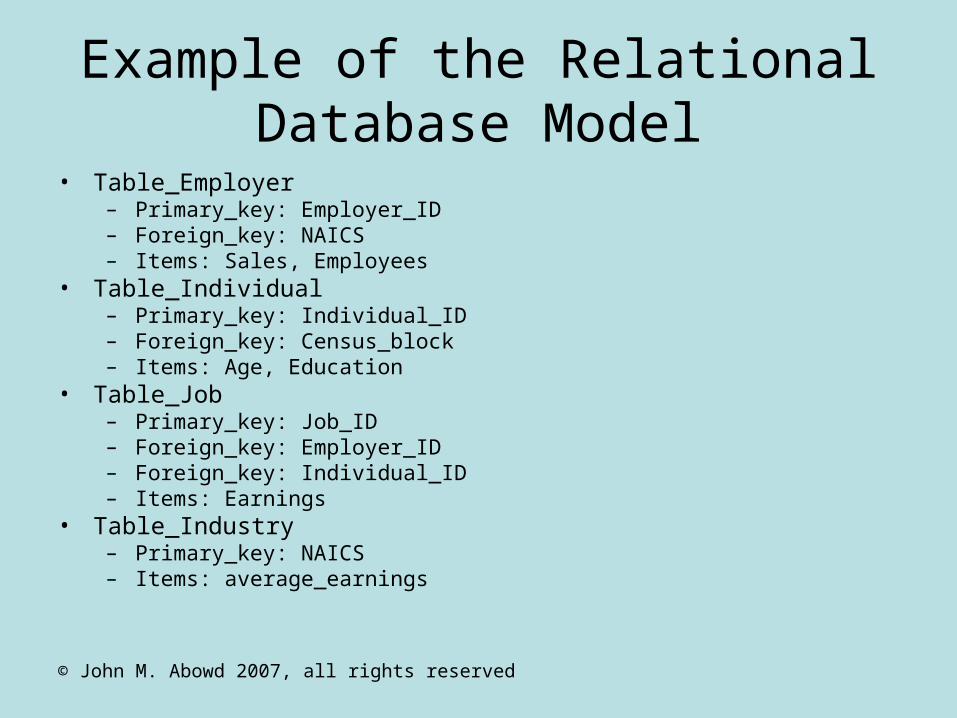
Example of the Relational Database Model

• Table_Employer– Primary_key: Employer_ID– Foreign_key: NAICS– Items: Sales, Employees

• Table_Individual– Primary_key: Individual_ID– Foreign_key: Census_block– Items: Age, Education

• Table_Job– Primary_key: Job_ID– Foreign_key: Employer_ID– Foreign_key: Individual_ID– Items: Earnings

• Table_Industry– Primary_key: NAICS– Items: average_earnings


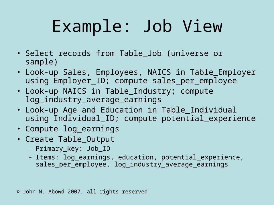
Example: Job View

• Select records from Table_Job (universe or sample)• Look-up Sales, Employees, NAICS in Table_Employer

using Employer_ID; compute sales_per_employee• Look-up NAICS in Table_Industry; compute

log_industry_average_earnings• Look-up Age and Education in Table_Individual using

Individual_ID; compute potential_experience• Compute log_earnings• Create Table_Output

– Primary_key: Job_ID– Items: log_earnings, education, potential_experience,

sales_per_employee, log_industry_average_earnings


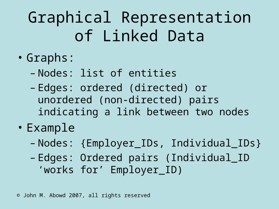
Graphical Representation of Linked Data

• Graphs: – Nodes: list of entities– Edges: ordered (directed) or unordered (non-

directed) pairs indicating a link between two nodes

• Example– Nodes: {Employer_IDs, Individual_IDs}– Edges: Ordered pairs (Individual_ID ‘works

for’ Employer_ID)


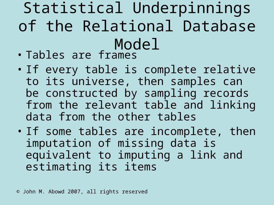
Statistical Underpinnings of the Relational Database Model

• Tables are frames• If every table is complete relative to its

universe, then samples can be constructed by sampling records from the relevant table and linking data from the other tables

• If some tables are incomplete, then imputation of missing data is equivalent to imputing a link and estimating its items


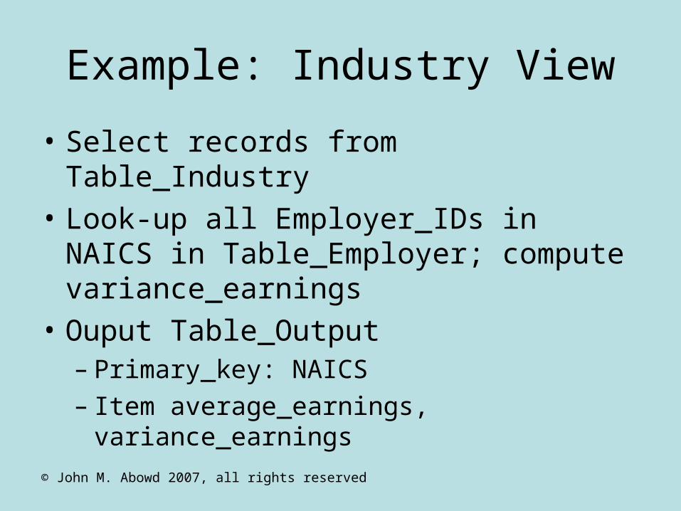
Example: Industry View

• Select records from Table_Industry

• Look-up all Employer_IDs in NAICS in Table_Employer; compute variance_earnings

• Ouput Table_Output– Primary_key: NAICS– Item average_earnings, variance_earnings


Estimating Models from Linked Files

• Linked files are usually analyzed as if the linkage were without error

• Most of this class focuses on such methods

• There are good reasons to believe that this assumption should be examined more closely


Lahiri and Larsen

• Consider regression analysis when the data are imperfectly linked

• See JASA article March 2005 for full discussion


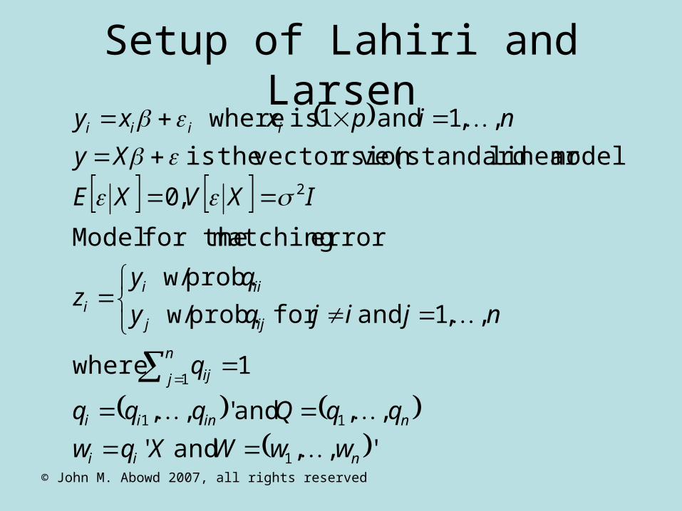
Setup of Lahiri and Larsen

',, and '

,, and ',,

1 where

,,1 and for prob. w/

prob. w/

error matching for the Model

,0

model)linear (standardrsion vector ve theis

,,1 and 1is where

1

11

1

2

nii

ninii

n

j ij

ijj

iiii

iiii

wwWXqw

qqQqqq

q

njijqy

qyz

IXVXE

Xy

nip xxy


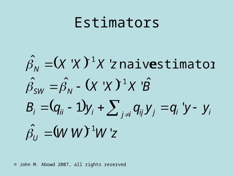
Estimators

zWWW

yyqyqyqB

BXXX

zXXX

U

iiij jijiiii

NSW

N

''ˆ

'1

ˆ''ˆˆ

estimator naive ''ˆ

1

1

1


Problem: Estimating B

2001)JASA Rubin andLarsen (see

models mixture using estimate :2 Technique

10a) lecture (see

algorithm EM theusing estimate :1 Technique

use tomodelSunter -Fellegi thehave wey,Fortunatel

theof estimates needs one estimate To

ij

ij

ij

q

q

qB


Does It Matter?

• Yes

• The bias from the naïve estimator is very large as the average qii goes away from 1.

• The SW estimator does better.

• The U estimator does very well, at least in simulations.


Graph-based Estimation Models

• Abowd-Schmutte paper


Building Integrated Labor Market Data

• Examples from the LEHD infrastructure files• Analysis can be done using workers, jobs or

employers as the basic observation unit• Want to model heterogeneity due to the workers

and employers for job level analyses• Want to model heterogeneity due to the jobs and

workers for employer level analyses• Want to model heterogeneity due to the jobs and

employers for individual analyses


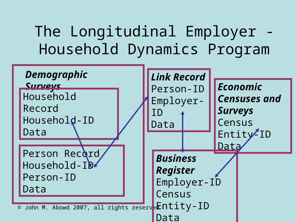
The Longitudinal Employer - Household Dynamics Program

Link RecordPerson-ID Employer-IDData

Business Register Employer-IDCensus Entity-IDData

Economic Censuses and SurveysCensus Entity-ID Data

Demographic Surveys

Household RecordHousehold-IDData

Person Record Household-IDPerson-IDData


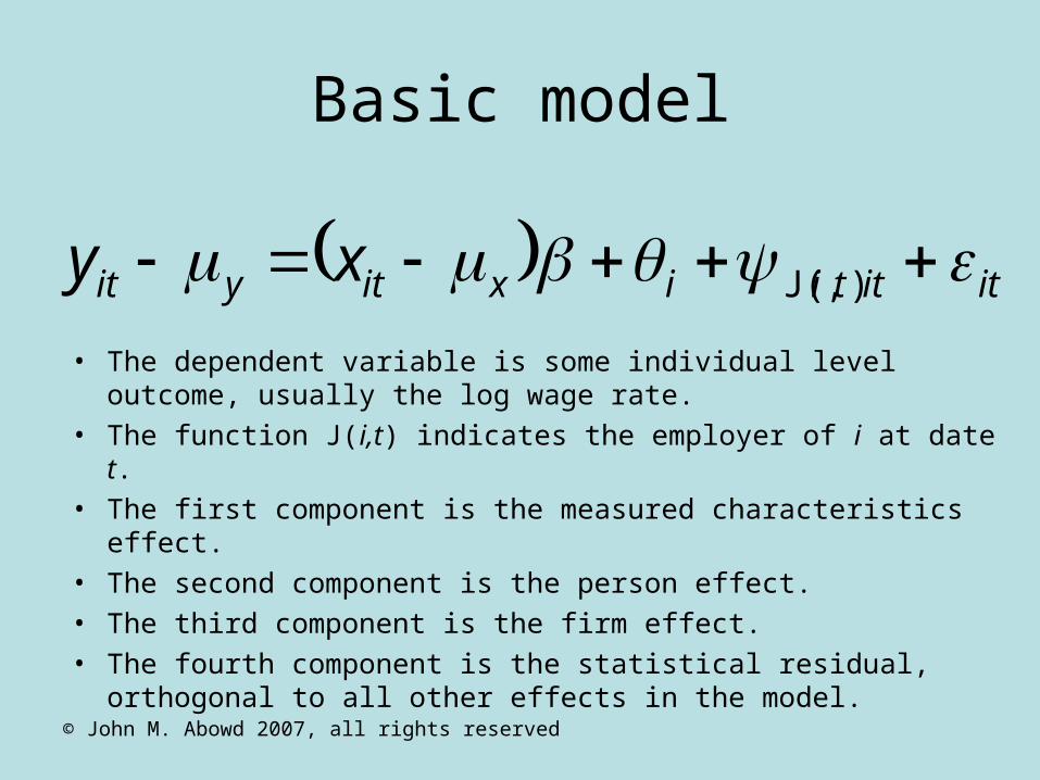
Basic model

itittiixityit xy ),J(

• The dependent variable is some individual level outcome, usually the log wage rate.

• The function J(i,t) indicates the employer of i at date t.• The first component is the measured characteristics effect.• The second component is the person effect.• The third component is the firm effect.• The fourth component is the statistical residual, orthogonal to all

other effects in the model.


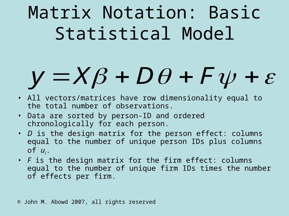
Matrix Notation: Basic Statistical Model

FDXy• All vectors/matrices have row dimensionality equal to the total

number of observations.• Data are sorted by person-ID and ordered chronologically for each

person.• D is the design matrix for the person effect: columns equal to the

number of unique person IDs plus columns of ui.• F is the design matrix for the firm effect: columns equal to the

number of unique firm IDs times the number of effects per firm.


Estimation by Fixed-effect Methods

• The normal equations for least squares estimation of fixed person, firm and characteristic effects are very high dimension.

• Estimation of the full model by either fixed-effect or mixed-effect methods requires special algorithms to deal with the high dimensionality of the problem.


Least Squares Normal Equations

• The full least squares solution to the basic estimation problem solves these normal equations for all identified effects.

yF

yD

yX

FFDFXF

FDDDXD

FXDXXX

'

'

'

'''

'''

'''


Identification of Effects

• Use of the decomposition formula for the industry (or firm-size) effect requires a solution for the identified person, firm and characteristic effects.

• The usual technique of eliminating singular row/column combinations from the normal equations won’t work if the least squares problem is solved directly.


Identification by Grouping• Firm 1 is in group g = 1.• Repeat until no more persons or firms are added:

– Add all persons employed by a firm in group 1 to group 1– Add all firms that have employed a person in group 1 to group

1

• For g= 2, ..., repeat until no firms remain:– The first firm not assigned to a group is in group g.– Repeat until no more firms or persons are added to group g:

• Add all persons employed by a firm in group g to group g.• Add all firms that have employed a person in group g to group g.

• Identification of : drop one firm from each group g.• Identification of : impose one linear restriction • Software

0,

ti

i

http://vrdc.ciser.cornell.edu/news/?p=140


Normal Equations after Group Blocking

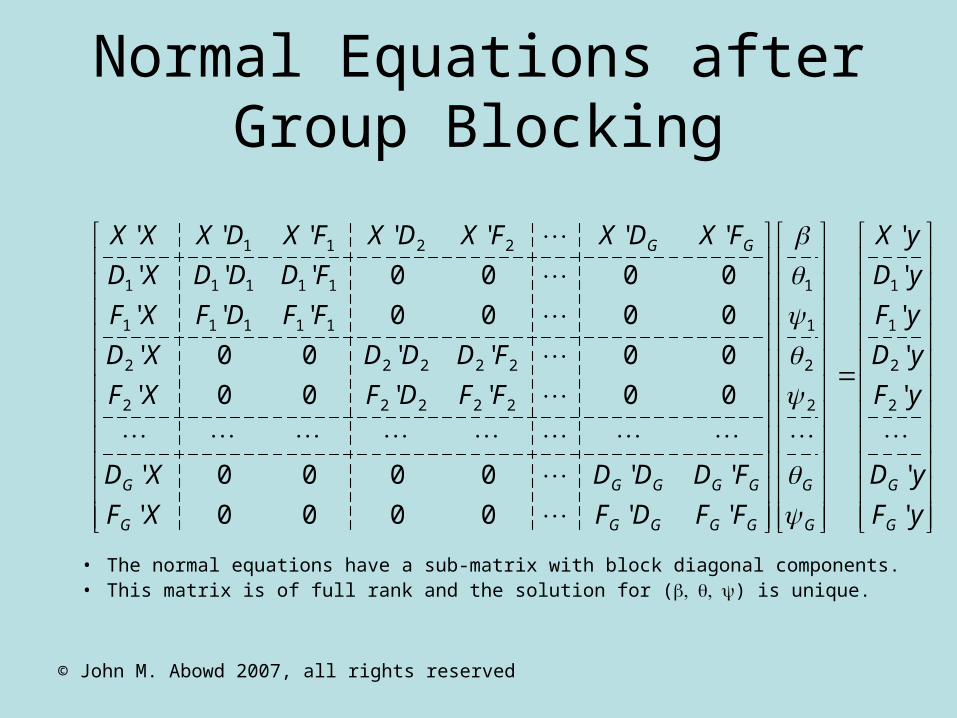
• The normal equations have a sub-matrix with block diagonal components. • This matrix is of full rank and the solution for () is unique.

yF

yD

yF

yD

yF

yD

yX

FFDFXF

FDDDXD

FFDFXF

FDDDXD

FFDFXF

FDDDXD

FXDXFXDXFXDXXX

G

G

G

G

GGGGG

GGGGG

GG

'

'

'

'

'

'

'

''0000'

''0000'

00''00'

00''00'

0000'''

0000'''

'''''''

2

2

1

1

2

2

1

1

22222

22222

11111

11111

2211


Necessity of Identification Conditions

• For necessity, we want to show that exactly N+J-G person and firm effects are identified (estimable), including the grand mean y. .

• Because X and y are expressed in deviations from the mean, all N effects are included in the equation but one is redundant because both sides of the equation have a zero mean by construction.

• So the grand mean plus the person effects constitute N effects.• There are at most N + J-1 person and firm effects including the grand mean. • The grouping conditions imply that at most G group means are identified (or, the

grand mean plus G-1 group deviations).

• Within each group g, at most Ng and Jg-1 person and firm effects are identified.

• Thus the maximum number of identifiable person and firm effects is:

g

gg JNGJN 1


Sufficiency of Identification Conditions

• For sufficiency, we use an induction proof.• Consider an economy with J firms and N workers.

• Denote by E[yit] the projection of worker i's wage at date t on the column space generated by the person and firm identifiers. For simplicity, suppress the effects of observable variables X

),J(E tiiyity • The firms are connected into G groups, then all effects j, in

group g are separately identified up to a constraint of the form:

0

group

gj

jjw


Sufficiency of Identification Conditions II

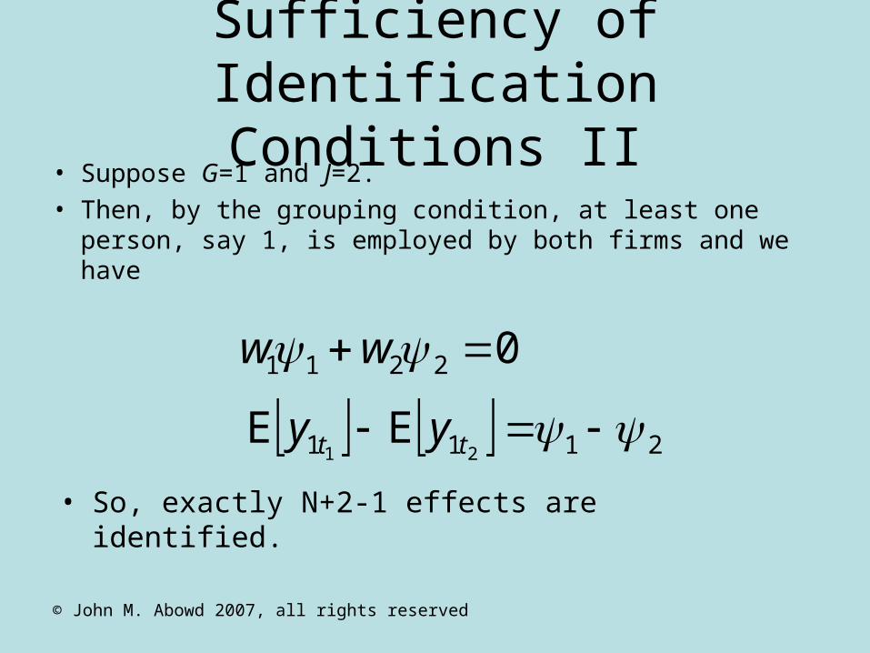
• Suppose G=1 and J=2.• Then, by the grouping condition, at least one person, say

1, is employed by both firms and we have

02211 ww

2111 21EE tt yy

• So, exactly N+2-1 effects are identified.


Sufficiency of Identification Conditions III

• Next, suppose there is a connected group g with Jg firms and exactly Jg -1 firm effects identified.

• Consider the addition of one more connected firm to such a group. • Because the new firm is connected to the existing Jg firms in the

group there exists at least one individual, say worker 1 who works for a firm in the identified group, say firm Jg, at date 1 and for the supplementary firm at date 2. Then, we have two relations

• So, exactly Jg effects are identified with the new information.

011 gg

g

JJJg

gg ww

111 21EE

gg JJtt yy


Characteristics of the Groups

Largest Group

Second Largest Group

Average of All Other Groups

Total of All Groups

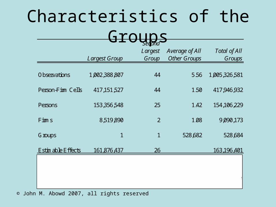
Observations 1,002,388,807 44 5.56 1,005,326,581

Person-Firm Cells 417,151,527 44 1.50 417,946,932

Persons 153,356,548 25 1.42 154,106,229

Firms 8,519,890 2 1.08 9,090,173

Groups 1 1 528,682 528,684

Estimable Effects 161,876,437 26 163,196,401Notes: The "pooled" data are comprised of annual observations from California, Colorado, Florida, Illinois, Iowa, Kansas, Maine, Maryland, Minnesota, Missouri, Montana, North Carolina, New Jersey, New Mexico, Oklahoma, Oregon, Pennsylvania, Texas, Virginia, Washington, West Virginia, and Wisconsin over the period 1990-2003. No single state contributed observations for all years. See Table 1. Sources: Author's calculations using the LEHD Program data base.


Estimation by Direct Solution of Least Squares

• Once the grouping algorithm has identified all estimable effects, we solve for the least squares estimates by direct minimization of the sum of squared residuals.

• This method, widely used in animal breeding and genetics research, produces a unique solution for all estimable effects.


FFDFXF

FDDDXD

FXDXXX

'''

'''

'''

of elements diagonal

ZFDXy 2/12/1||

2/12/1 and || FDXZ

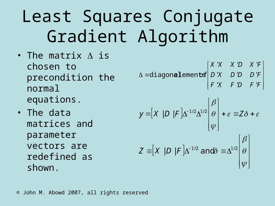
Least Squares Conjugate Gradient Algorithm

• The matrix is chosen to precondition the normal equations.

• The data matrices and parameter vectors are redefined as shown.


LSCG (II)

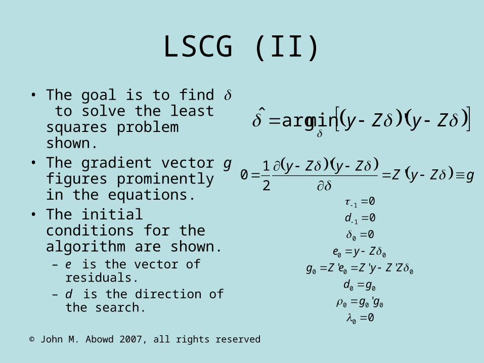
• The goal is to find to solve the least squares problem shown.

• The gradient vector g figures prominently in the equations.

• The initial conditions for the algorithm are shown.– e is the vector of residuals.– d is the direction of the

search.

ZyZy 'minargˆ

gZyZZyZy

''

2

10

0

'

'''

0

0

0

0

000

00

000

00

0

1

1

gg

gd

ZZyZeZg

Zye

d


LSCG (III)

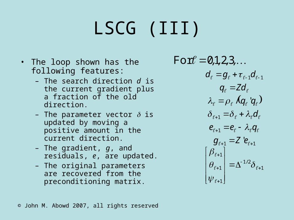
• The loop shown has the following features:– The search direction d is the

current gradient plus a fraction of the old direction.

– The parameter vector is updated by moving a positive amount in the current direction.

– The gradient, g, and residuals, e, are updated.

– The original parameters are recovered from the preconditioning matrix.

12/1

1

1

1

11

1

1

11

'

'/

eZg

qee

d

qq

Zdq

dgd

,,,, 3210For


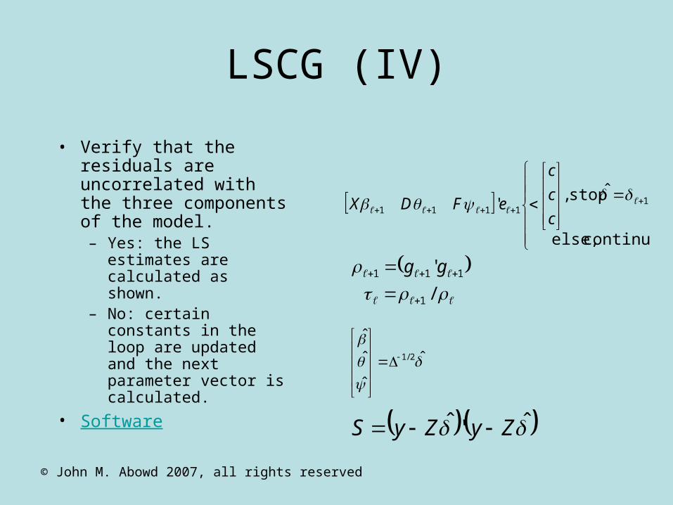
LSCG (IV)

• Verify that the residuals are uncorrelated with the three components of the model.– Yes: the LS estimates

are calculated as shown.

– No: certain constants in the loop are updated and the next parameter vector is calculated.

• Software

continue else,

ˆ stop ,' 1

1111

c

c

c

eFDX

/

'

1

111

gg

ˆ

ˆ

ˆ

ˆ2/1

ˆ'ˆ ZyZyS



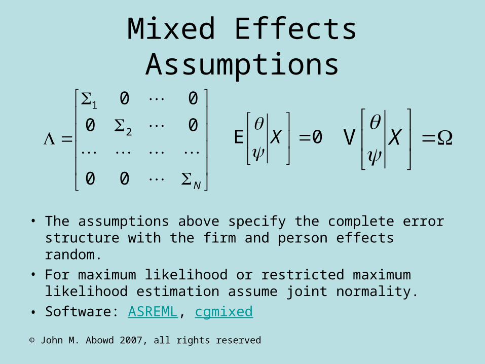
Mixed Effects Assumptions

• The assumptions above specify the complete error structure with the firm and person effects random.

• For maximum likelihood or restricted maximum likelihood estimation assume joint normality.

• Software: ASREML, cgmixed

N

00

00

00

2

1

0E

X

X

V

http://www.ciser.cornell.edu/FAQ/ASReml/ASReml_Documentation.shtml



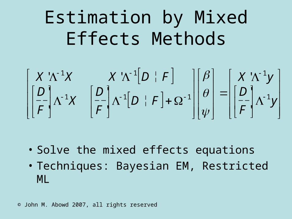
Estimation by Mixed Effects Methods

• Solve the mixed effects equations

• Techniques: Bayesian EM, Restricted ML

yF

DyX

FDF

DX

F

DFDXXX

1

1

111

11

'

''

'

'

'

'''


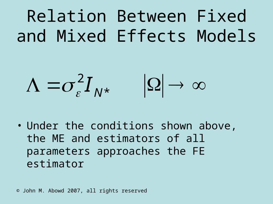
Relation Between Fixed and Mixed Effects Models

• Under the conditions shown above, the ME and estimators of all parameters approaches the FE estimator

*2

NI


Correlated Random Effects vs. Orthogonal Design

• Orthogonal design means that characteristics, person design, firm design are orthogonal.

• Uncorrelated random effects means that is diagonal.

designseffect -firm andeffect -person orthogonal 0

designeffect -firm and sticscharacteri personal orthogonal 0'

designeffect -person and sticscharacteri personal orthogonal 0'

D'F

FX

DX


Software

• SAS: proc mixed• ASREML• aML• SPSS: Linear Mixed Models• STATA: xtreg, gllamm, xtmixed• R: the lme() function• S+: linear mixed models• Gauss• Matlab• Genstat: REML • Grouping (connected sub-graphs)


Documents

© John M. Abowd 2007, all rights reserved Statistical Tools for Data Integration John M. Abowd April 2007