Embed Size (px)
Citation preview
Jet Energy Scale Studies and the Search for the
Standard Model Higgs Boson in the
Channel ZH → ννbb at DØ
Lydia Mary Isis Lobo
Imperial College London
A thesis submitted in fulfilment of
the requirements for the degree of
Doctor of Philosophy
of the University of London
and the Diploma of Imperial College
November 2006
Jet Energy Scale Studies and the Search for the
Standard Model Higgs Boson in the
Channel ZH → ννbb at DØ
Lydia Mary Isis Lobo
Imperial College London
November 2006
ABSTRACT
The DØ experiment is based at the Tevatron, which is currently the world’s
highest-energy accelerator. The detector comprises three major subsystems: the
tracking system, the calorimeter and the muon detector. Jets, seen in the calorime-
ter, are the most common product of the proton-proton interactions at 2TeV. This
thesis is divided into two parts. The first part focuses on jets and describes the
derivation of a jet energy scale using pp →(Z + jets) events as a cross-check of the
official DØ jet energy scale (Versions 4.2 and 5.1) which is derived using pp→ γ+jets
events. Closure tests were also carried out on the jet energy calibration as a further
verification. Jets from b-quarks are commonly produced at D��O, readily identified
and are a useful physics tool. These require a special correction in the case where
the b-jet decays via a muon and a neutrino. Thus a semileptonic correction was also
derived as an addition to the standard energy correction for jets.
The search for the Higgs boson is one of the largest physics programmes at
D��O. The second part of this thesis describes a search for the Standard Model Higgs
boson in the ZH → ννbb channel in 52fb−1 of data. The analysis is based on a
sequence of event selection criteria optimised on Monte Carlo event samples that
simulate four light Higgs boson masses between 105 GeV and 135GeV and the main
backgrounds. For the first time, the data for the analysis are selected using new
acoplanarity triggers and the b-quark jets are selected using the DØ neural net b-jet
tagging tool. A limit is set for σ(pp→ ZH) × Br(H → bb).

3
Acknowledgements
“Sometimes our light goes out but is blown into flame by another human
being. Each of us owes deepest thanks to those who have rekindled this
light.” Albert Schweitzer
Life is most interesting, retrospectively, when things don’t work or you make
mistakes. This journey to completing my thesis has been difficult, tiring, enlight-
ening and rewarding. When I started, I assumed that I was here to learn all about
high energy physics and scientific writing. I didn’t realise then how much more
important would be all the other things I learnt from the people I have been lucky
enough to meet and to work with. I know now that a PhD is not just about doing
a few years work and then writing it all down. It’s about developing an instinct for
when things aren’t as they seem, learning to ask the right questions and realising
that there are no silly questions, and motivating oneself to persist when things are
at their most frustrating.
Although I now leave behind science as my daily activity, I will always be a
physicist in mind with an immutable scientific disposition. In my heart, I hold dear
the many happy memories of the people I’ve encountered, and feel an enormous
sense of gratitude for their help, support and wisdom. Most importantly, I would
like to thank Gavin Davies, my supervisor, for his practical guidance, seemingly
unlimited patience, and unwavering support. Gavin, you have been a better super-
visor than I could ever have hoped for and I have learned more than physics, through

4
observing your leadership of the DØ Group at Imperial. I would also like to thank
Rachel Padman for her fantastic support as my Director of Studies throughout my
undergraduate years. I have been incredibly lucky to have had you both as mentors.
Thanks also to Trevor Bacon for reading my thesis so meticulously.
My deepest thanks go to my mother and father and to David, who have sup-
ported me in every way possible for so long: feeding, watering and sheltering me,
providing endless encouragement, showing boundless faith in my abilities and for
reading my thesis. I’d also like to thank Grandma, Grandpa and Nana, my grandpar-
ents, no longer with us, and my Aunt Moira, for their continuous support throughout
my studies.
At Imperial, many thanks must firstly go to Michele Petteni and Tim Scanlon
for all their practical help and patience in answering my questions. Without Ray
Beuslinck, Kostas Georgiou and Bill Cameron to solve so willingly my frequent
computer problems, I wonder if I would have made it through the past few years!
At Fermilab too, I had the pleasure to work with some very dedicated people and
I’d like to thank Ia Iashvilli for her help and guidance with my work on the jet
energy scale, Anna Goussiou for her help with the Jet Energy Scale and eflow, and
Jon Hays for his guidance on eflow. I would also like to thank Daniela Bauer, Claus
Buzello, Philip Perea, and Amber Jenkins for their ready help whenever I asked.
Also, thanks to Paula Brown for her ready smile, advice and help.
Thanks must also go to PPARC for their studentship grant and the Imperial
HEP group for the opportunity to be part of the group; together these have enabled
me to work in London and Chicago on an international experiment and to meet
people from so many different backgrounds.
At both Fermilab and Imperial I have made many friends of whom I have count-
less fond memories. I will miss the teatime banter in the trailers with often six or
more nationalities made all the more amusing by cultural communication differ-
ences. Help and a welcome reminder of the UK was always forthcoming from the

5
fermifogies lot: Tamsin, Emily, Anant, Martin G, Dustin, Paul, Matt, James, Ben,
Simon, Stephen, Kyle, Nicola, Gavin, Tim, Phil, Amber, Philip and Satish (hon-
orary members). Anatoly, Robert, Raymond and Sarosh, thanks for the trips to
Panera, broadening my film appreciation and the extensive commentary on Ameri-
can culture. I will always smile when I think of my house and office mates Amber
and Alex - thank you for the calm and making Fermilab feel like home. My time in
London would not have been the same without the Imperial bunch. Special thanks
to Lisa and Helen H. for all their tea and pearls of PhD wisdom that helped during
the more difficult parts. I would also like to thank my old friends, Alex, Bee, Ruth,
Lucy, Laura, Debjani, Nick HJ, Nasrin and Michelle - you’ve known me most of my
life, thanks for all your support, advice and cheeriness when the frustrations seemed
never-ending. There are many more I’d like to include, but there isn’t space, you
know who you are - thank you to you too. I wish you all luck, health and happiness
in your future endeavours.

6
Contents
Abstract 2
Acknowledgements 3
Contents 6
List of Figures 10
List of Tables 17
Preface 20
Chapter 1. The Standard Model and the Higgs Boson 23
1.1 Introduction 23
1.2 The Standard Model 24
1.3 Matter and its Interactions 24
1.4 Gauge Theories 25
1.4.1 Non-Abelian Gauge Transformations 28
1.5 Electroweak Theory 29
1.6 The Higgs Mechanism 32
1.7 Current Limits on the Higgs Mass 36
1.7.1 Limits from Theory 36
1.7.2 Limits from Indirect Methods 37
1.7.3 Limits from Direct Methods 38
1.8 Conclusions 40

Contents 7
Chapter 2. Experimental Apparatus 41
2.1 The Tevatron 42
2.1.1 Production, storage and pre-acceleration of protons and anti-
protons 42
2.1.2 Particle Acceleration 43
2.1.3 Tevatron Performance 44
2.2 The DØ Detector 44
2.2.1 The Detector Coordinate System and Units 45
2.2.2 Central Tracking System 47
2.2.3 Calorimeter and pre-shower 50
2.2.4 Muon System 55
2.2.5 The Forward Proton Detector 59
2.2.6 Luminosity Monitor 59
2.2.7 Trigger System and Data Acquisition System 60
2.2.8 Object Identification 62
2.2.9 Overall Current Detector Performance and Status 70
Chapter 3. The Jet Energy Scale 72
3.1 Introduction 72
3.2 The Jet Energy Scale 73
3.3 Jet Response 76
3.3.1 Missing ET Projection Fraction Method 76
3.3.2 Jet Response Calculation 82
3.3.3 Closure Tests 89
3.4 Discussion 91
3.5 Conclusion 94
Chapter 4. The Calorimeter Response to Semileptonic Decays and
Energy Flow 95
4.1 Introduction 95
4.2 Semileptonic Decays: Muons 97
4.2.1 Definition of the Semileptonic Correction 97
Contents 8
4.2.2 Vector Correction 108
4.2.3 Closure Test: Effects on Mass Resolutions 109
4.2.4 Discussion 111
4.3 Energy Flow: Electromagnetic Calorimeter Calibration 112
4.3.1 Towards a Working Algorithm 113
4.3.2 Event Samples and Selection Criteria 113
4.3.3 Electromagnetic Scale 116
4.4 Conclusions 120
Chapter 5. Search for the Standard Model Higgs Boson 123
5.1 Introduction 123
5.2 Data and Monte Carlo Event Samples Used 126
5.2.1 Data Set 126
5.2.2 Monte Carlo 126
5.2.3 Trigger Terms 127
5.3 Event Selection 131
5.3.1 Basic Event Selection 132
5.3.2 Instrumental and Other Selection Criteria 140
5.3.3 Background Estimation 144
5.3.4 Taggability Corrections 146
5.4 Monte Carlo Optimisation and b-tagging 152
5.4.1 B-tagging 153
5.4.2 MINUIT Optimisation of Certain Variables 156
5.4.3 Results of Optimisation of Event Selection 157
5.4.4 Summary of Event Selection 158
5.5 Errors 158
5.6 Limit on σ(pp→ ZH) ×Br(H → bb) 160
5.7 Conclusions 164
Chapter 6. Conclusions 166
6.1 Further work and the future 169
Appendix A. Binning of Data and Monte Carlo Response in E’ 172

Contents 9
Appendix B. Analysis cutflow tables 175
Appendix C. Event Display Plots 180
10
List of Figures
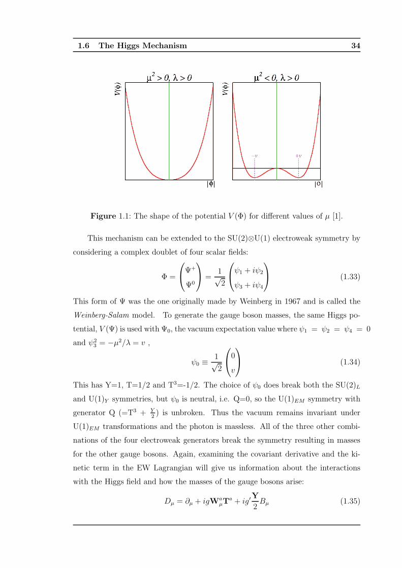
1.1 The shape of the potential V (Φ) for different values of µ [1]. 34
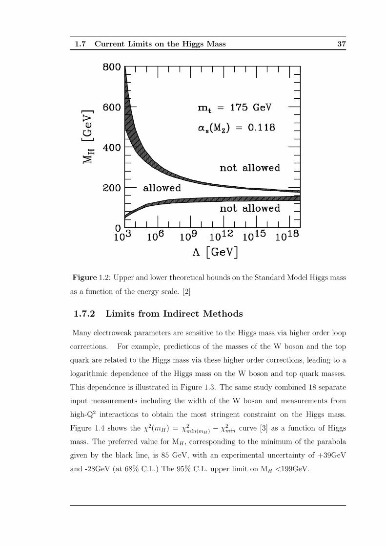
1.2 Upper and lower theoretical bounds on the Standard Model Higgs mass
as a function of the energy scale. [2] 37
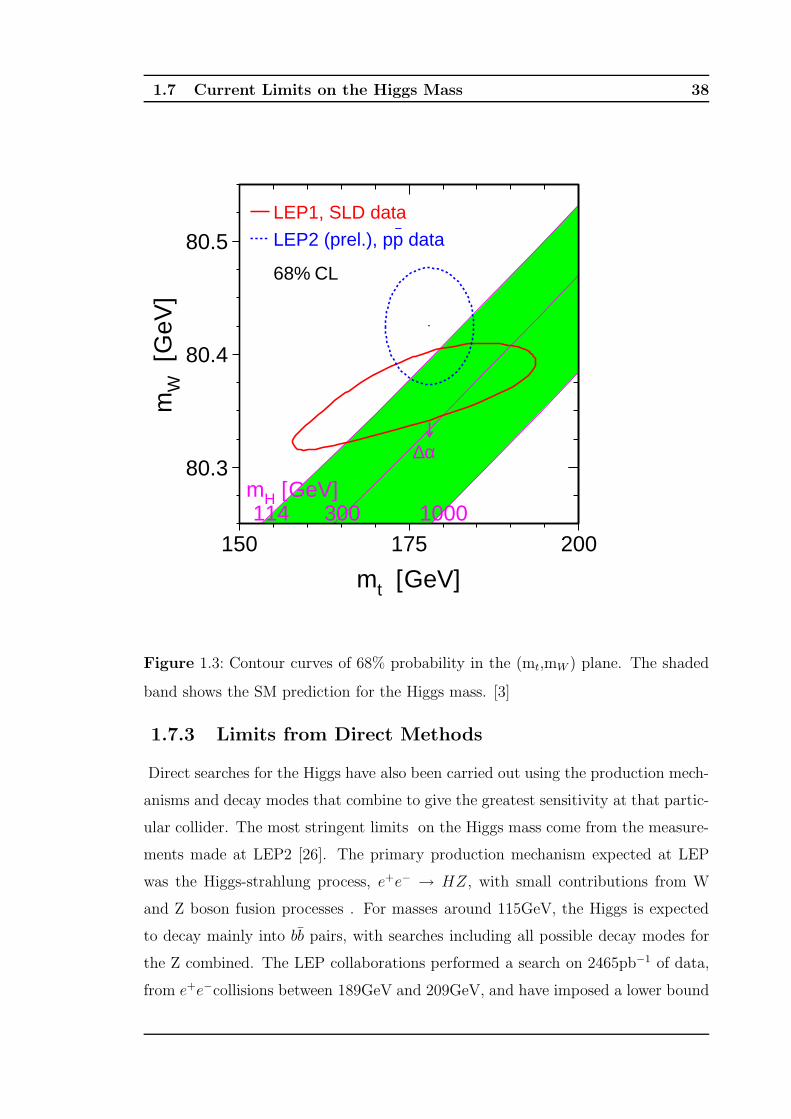
1.3 Contour curves of 68% probability in the (mt,mW ) plane. The shaded
band shows the SM prediction for the Higgs mass. [3] 38
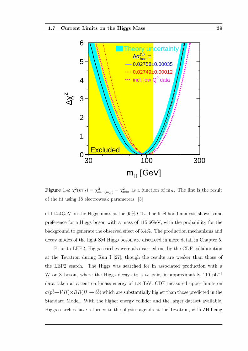
1.4 χ2(mH) = χ2min(mH ) − χ2
min as a function of mH . The line is the result of
the fit using 18 electroweak parameters. [3] 39
2.1 The Tevatron Accelerator Complex 42
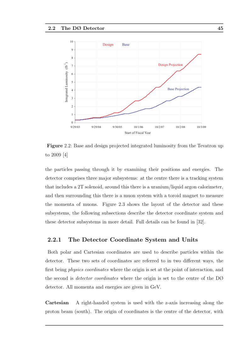
2.2 Base and design projected integrated luminosity from the Tevatron up
to 2009 [4] 45
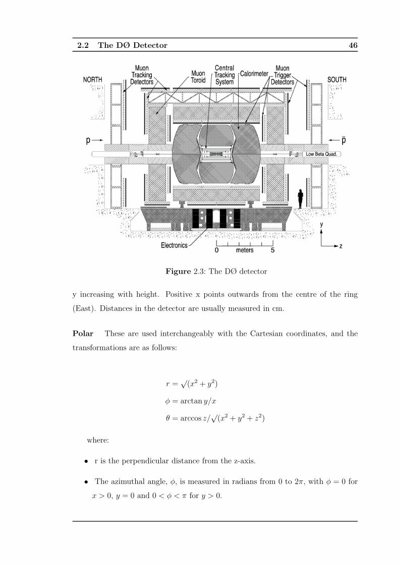
2.3 The DØ detector 46
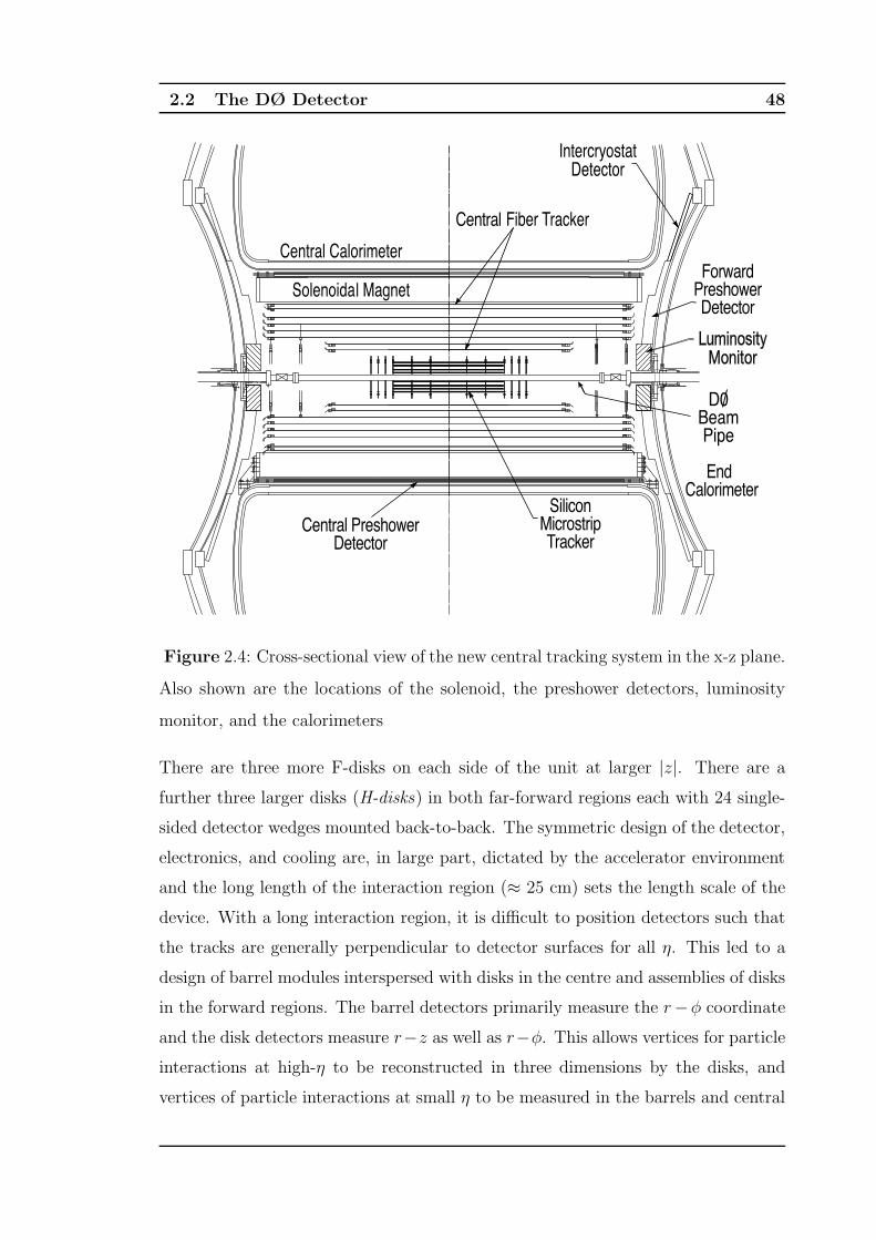
2.4 Cross-sectional view of the new central tracking system in the x-z plane.
Also shown are the locations of the solenoid, the preshower detectors,
luminosity monitor, and the calorimeters 48
2.5 The disk and barrel design of the silicon microstrip tracker. 49
2.6 Isometric view of the central and two end calorimeters 51
2.7 Schematic view of a portion of the DØ calorimeters showing the trans-
verse and longitudinal segmentation pattern. The shading pattern indi-
cates groups of cells ganged together for signal readout. The rays mark
pseudorapidity intervals from the centre of the detector. 52
2.8 Schematic view of the liquid argon gap and signal board unit cell for the
calorimeter 53
List of Figures 11
2.9 Exploded view of the muon detectors 55
2.10 Overview of the DØ trigger and data acquisition systems 60
2.11 Block diagram of the DØ L1 and L2 trigger systems. The arrows show
the flow of trigger related data 61
2.12 The DØ detector performance for Run II 71
3.1 Showering profile for central calorimeter jets of R=0.5 in the data, after
offset and baseline energy subtraction 75
3.2 (Z + jets) E-E′ mappings, top to bottom: CC, ICR, EC. 78
3.3 Monte Carlo response for the EC, binned in E′ for 75GeV<E′ <105GeV
(top left) to E′ >250GeV (bottom right). 83
3.4 Response (∆φ ≥ 3.0) with a quadratic log fit as motivated in the text,
before cryostat factor correction against a) E′(upper) and b) E (lower) 84
3.5 Cryostat Factor 85
3.6 Response (∆φ ≥ 3.0) with a quadratic log fit as motivated in the text,
after cryostat factor correction against a) E′ (upper) and b) E (lower) 86
3.7 Data response with a quadratic log fit, for various ∆φ cuts: a)∆φ ≥2.8, b)∆φ ≥ 2.9, c)∆φ ≥ 3.0, d)∆φ ≥ 3.1 after cryostat factor correction. 88
3.8 Monte Carlo response with a quadratic log fit, for various ∆φ cuts:
a)∆φ ≥ 2.8, b)∆φ ≥ 2.9, c)∆φ ≥ 3.0, d)∆φ ≥ 3.1 after cryostat factor
correction. 88
3.9 Monte Carlo closure tests: histograms of Rapprox for jets before JetCorr
corrections for all regions (top left), and broken down into the CC (top
right), ICR (bottom left) and EC (bottom right). 90
3.10 Monte Carlo closure tests: histograms of Rapprox for jets after JetCorr
corrections for all regions (top left), and broken down the CC (top right),
ICR (bottom left) and EC (bottom right). 90
3.11 Data closure tests: Rapprox for jets before JetCorr corrections for all re-
gions (top left), and broken down into the CC (top right), ICR (bottom
left) and EC (bottom right). Note the inability to fit satisfactorily a gaus-
sian curve to the data in the EC (bottom right) due to the low statistics
as noted earlier in this subsection. 91
List of Figures 12
3.12 Data closure tests: Rapprox for jets after JetCorr corrections for all regions
(top left), and broken down into the CC (top right), ICR (bottom left)
and EC (bottom right). 92
3.13 Response plot for (γ + jets) events. Solid lines represent the response
from R=0.5 jets, and the dashed lines represent the response from R=0.7
jets. [5] 93
4.1 △R plots between the main objects in the event. △R(reconstructed
muon, generator muon), (left). △R(reconstructed jet, generator b-quark),
(middle). △R(reconstructed jet, reconstructed muon), (end). 100
4.2 Generator level muon energy, (Eparticle)µ, as a function of reconstructed
muon energy, Erecoµ . Solid line corresponds to y=x. The points show the
scatter of data points, while the cross-hairs represent the midpoints of
the same data points, binned. 101
4.3 Typical correction factor distribution (Muon energy bin 28GeV < Eµ <
32 GeV). 101
4.4 Correction factor as a function of the reconstructed muon energy for
inclusive decays. Also shown is the correction factor in terms of generator
level information. 102
4.5 Correction factor as a function of reconstructed muon energy for Eb−jet <
50 GeV and Eb−jet > 50 GeV. 103
4.6 Correction factor as a function of reconstructed muon energy for prelT >
1GeV and prelT < 1GeV 103
4.7 Reconstructed prelT distribution for direct, cascade and inclusive decays 104
4.8 Correction factor as a function of reconstructed muon energy for direct
(top) and cascade (bottom) decays 104
4.9 Correction factor as a function of reconstructed muon energy for direct
(top) and cascade (bottom) for prelT greater and less than 1 GeV. 105
4.10 Correction factor as a function of reconstructed muon energy for direct
(top) and cascade (bottom) for jet energy greater and less than 50 GeV. 106
4.11 Correction factor for direct decays for Ejet < 50GeV (upper fit values)
and Ejet > 50GeV (lower fit values), split by prelT > 1GeV (top) and
prelT < 1GeV (bottom). 106
List of Figures 13
4.12 Correction factor for cascade decays for Ejet < 50GeV and Ejet > 50GeV,
split by jet energy for prelT > 1GeV (top) and prel
T < 1GeV (bottom). In
each plot the upper fit values are for Ejet > 50GeV and the lower values
are for Ejet < 50GeV 107
4.13 Neutrino energy from generator level information and the neutrino energy
derived from the fit to the correction factor (top), difference between the
two neutrino energies (bottom). 108
4.14 △R between the b-quarks and the b-jets corrected with a)the scalar and
b)the vector semileptonic corrections. 109
4.15 Dijet Mass Resolutions for H → bb 110
4.16 Ecluster/ptrack against △R between the cluster and the matched track for
data (left) and MC (right) 116
4.17 Electromagnetic scale for data. 118
4.18 Electromagnetic scale for MC. 118
4.19 Cluster invariant mass after correction. The events above 5GeV in (a)
are due to combinatorics. 119
4.20 a) Cluster energy/track momentum against track momentum, b) Cluster
energy (GeV) against electron track momentum (GeV) for various η bins
for data. 120
4.21 MC jet ET resolution for cone R=0.7. Upper, blue points are for calorime-
ter jets only, lower, red points are for TrackCal jets. 122
5.1 Higgs production cross-sections (pb) at the Tevatron for the various pro-
duction mechanisms as a function of the Higgs mass, taken from [6]. 124
5.2 Feynman diagram of the associated production of a Higgs boson and a
vector boson. 125
5.3 Branching ratios of the dominant decay modes of the Standard Model
Higgs boson [7]. 125
5.4 Inclusive distribution of fired triggers for the v13 data set. 131

List of Figures 14
5.5 Distributions for the leading and next-to-leading jet in the event after
basic cuts. a)φ-distribution for leading jet, b)φ-distribution for next-to
leading jet, c)η-distribution for leading jet, d)η-distribution for next-to
leading jet, e)η − φ-distribution for leading jet and f)η − φ-distribution
for next-to leading jet. 134
5.6 E/T distributions after basic cuts and a two-jet requirement. Top left:
E/T Top right: E/T - φ which shows the asymmetry that is thought to
be due to calorimeter miscalibrations, instrumental backgrounds, trigger
effects and ’noise’ jets in the event. Bottom left: E/T x-component Bottom
right: E/T y-component. In addition to the asymmetry mentioned visible
in the φ distribution, the x and y-components show the a dip around
zero characteristic of some of the problems with DØ tracking. 135
5.7 ��HT distributions after basic cuts and a two-jet requirement. Top left: H/T
and top right: H/T φ distribution. Bottom left: x-component H/T distribu-
tion. Bottom right: y-component H/T distribution. 136
5.8 E/T φ distributions after basic cuts and after imposing varying E/T cuts.
Top left: E/T φ distribution. Top right: E/T φ distribution andE/T >30GeV.
Bottom left: E/T φ distribution and E/T >50GeV. Bottom right: E/T φ dis-
tribution and E/T >80GeV. It can be seen that the central asymmetry in
the φ-distribution decreases with increasing E/T cuts. 137
5.9 H/T φ distributions after basic cuts and after imposing varying H/T cuts.
Top left: H/T φ distribution after basic cuts. Top right: H/T φ distribution
and H/T >30GeV Bottom left: H/T φ distribution and H/T >50GeV Bottom
right: H/T φ distribution and H/T >80GeV. It can be seen that the H/T φ
distribution improves after imposing the H/T >80GeV cut. 138
5.10 E/T - φ distributions after basic cuts and with varying E/T cuts, for events
with no bad or noise jets 139
5.11 Distributions for the leading and next-to-leading jet in the event after ba-
sic cuts, for the muon-triggered sample. Distributions in the left column
are for the leading jet, and in the right column for the next-to-leading
jet. Top to bottom are shown the φ distributions, the η distributions and
the η − φ distributions. 141
List of Figures 15
5.12 E/T distributions after basic cuts and a two-jet requirement for the muon-
triggered sample. Top left: E/T . Top right: φ distribution. Bottom left:
x-component of the E/T distribution. Bottom right: y-component of the
E/T distribution. 142
5.13 H/T distributions after basic cuts and a two-jet requirement for the muon-
triggered sample. Top left: H/T . Top right: φ distribution. Bottom left:
x-component of the H/T distribution. Bottom right: y-component of the
H/T distribution. 143
5.14 Scatter plot of Asym(E/T , H/T ) against |trkE/T − trkE/T (dijet)|/trkE/T . Af-
ter all selection criteria except the two plotted. Top plot: data. Middle:
signal MC. Bottom: background MC (un-normalized). The central boxes
represent the signal region and the side boxes the ‘sideband’ regions. 145
5.15 Fits for MC, sideband and signal region (left, centre and right), with no tagga-
bility requirements, at least one taggable jet and two taggable jets (top, centre,
bottom). The lighter, yellow-shaded region represents the contribution to the
physics background from Wj/Wjj/Wbb events. The darker, blue-shaded re-
gion represents the contribution from Zj/Zjj/Zbb events. 147
5.16 Jet taggability in data as a function of φ (top), η (middle) and pT (bottom).148
5.17 Jet data taggability efficiency parameterised in η−pT 149
5.18 Fits for MC, sideband and signal region (left,centre and right) for two
taggable jets after taggability corrections. 150
5.19 Basic jet distributions for leading (left) and next-to-leading jet (right).
The lighter, yellow-shaded region represents the contribution to the physics
background from Wj/Wjj/Wbb events. The darker, blue-shaded region
represents the contribution from Zj/Zjj/Zbb events. 151
5.20 Missing energy distributions. Missing ET in units of GeV. The lighter,
yellow-shaded region represents the contribution to the physics back-
ground from Wj/Wjj/Wbb events. The darker, blue-shaded region rep-
resents the contribution from Zj/Zjj/Zbb events. 152
List of Figures 16
5.21 Distributions for missing HT , scalar HT , jet multiplicity and di-jet invari-
ant mass. Units of GeV. The lighter, yellow-shaded region represents the
contribution to the physics background from Wj/Wjj/Wbb events. The
darker, blue-shaded region represents the contribution from Zj/Zjj/Zbb
events. 153
5.22 Standard Model, observed and expected limits (pb) against MH (GeV). 162
5.23 Data event display of a ZH event candidate that passes all selection cuts.
Run number = 195258, event number = 3860440. On the left is shown
the calorimeter transverse energy in the η− φ plane. On the right is the
calorimeter and tracking view, as a projection in the x−y plane at z = 0.
Missing ET is shown in orange. 163
6.1 The ratio of the expected and observed 95% CL limits to the SM cross
section for the combined CDF and DØ analyses. 171
A.1 Data response for the EC, binned in E’ 172
A.2 Data response for the CC, binned in E’ 173
A.3 Monte Carlo response for the CC, binned in E’ 174
C.1 Data event display of a ZH event candidate that passes all selection cuts.
Run number = 195837, event number = 22994974 180
C.2 Data event display of a ZH event candidate that passes all selection cuts.
Run number = 195519, event number = 12633422 181
C.3 Data event display of a ZH event candidate that passes all selection cuts.
Run number = 194720, event number = 4671138 181
C.4 Data event display of a ZH event candidate that passes all selection cuts.
Run number = 194800, event number = 35678049 182

17
List of Tables
1.1 Summary of some of the properties of the three generations of matter
particles. [8] 24
1.2 Summary of some of the properties of the force-mediating particles of
the Standard Model. [8] 25
2.1 Some key operating characteristics of the Tevatron for Run II 44
2.2 Table of materials used in the central and end calorimeters and dimen-
sions of these layers. See Section 2.2.8 for explanation of χ0 and λA.
(*except 3rd layer: 0.05 × 0.05) 53
2.3 Momentum resolution parameters for the central and forward muon de-
tectors. [9] 58
2.4 Selection criteria for tight, medium and loose muons 65
3.1 Number of data and MC events passing the selection criteria 82
3.2 Data: variation of response with ∆φ cut where a, b and c are constants
of Equation 3.12. 87
3.3 Monte Carlo: variation of response with ∆φ cut where a, b and c are
constants of Equation 3.12. 87
3.4 Comparison of (Z + jets) and (γ + jets) response parameters, and cryo-
stat factors in data and Monte Carlo (Z + jets) and (γ + jets) event
samples. 93
4.1 Number of selected events for cascade and direct decays, with prelT >
1GeV and prelT < 1GeV. 99
List of Tables 18
4.2 Dijet masses, spreads of the distributions and resolutions for H → bb and
Z → bb MC samples after no JES correction, basic JES correction, and
full jet correction. The error on the means and RMS is approximately
0.5GeV. 110
4.3 Dijet mass Gaussian means, sigmas and resolutions for Z → bb events
with no correction, basic JES correction and basic + semileptonic correc-
tion. Errors on the means and sigmas are approximately 0.1GeV, except
for the case of two semileptonic decays where the error is approximately
1GeV due to lower statistics. 111
4.4 Details of the L1, L2 and L3 trigger requirements for the E7A 2RL3 RT3 RL5
and E7B 2RL3 RT3 RL5 114
4.5 Criteria for loose and tight road electrons 115
4.6 Numbers of events passing selection criteria for data and MC event samples117
4.7 Data and Monte Carlo EM scale parameters (refer to Equation 4.4).
Cluster invariant masses (GeV) before and after correction. 119
5.1 Details of the L1, L2 and L3 trigger requirements for the four acoplanarity
triggers used in this analysis. 128
5.2 Table of signal Monte Carlo event samples used. 129
5.3 Table of background Monte Carlo event samples used 130
5.4 Number of events obtained from fits to the QCD and non-QCD compo-
nents in data for different taggability conditions. 146
5.5 NN b-tagger operating points, and corresponding efficiencies, approxi-
mate fake rates and systematic uncertainties [10]. The JLIP equivalent
fake rates are quoted where available in brackets next to the NN b-tagger
quantity. 155
5.6 Summary of number of events after selection cuts, MH =115GeV, no
mass window, for comparison of the effect of replacing the JLIP tagger
with the NN tagger. 156
5.7 Variables optimised using MINUIT for MH = 115GeV. 157
5.8 Estimation of the number of instrumental background events after double
medium JLIP tagging and double loose NN tagging. 158

List of Tables 19
5.9 Systematic uncertainties due to corrections, taggability fits, b-tagging
and background estimation for all background samples and for MH =
115GeV, and a double loose NN b-tag. 159
5.10 Number of expected and observed events, channel and signal accep-
tance (includes Z → νν branching ratio), sensitivity, observed and ex-
pected cross-section limit for three mass points MH = 105GeV, 115GeV,
125GeV, 135GeV. 161
B.1 Part I: Selection Cut Efficiencies (%) for the data, MC signal (MH =
115GeV) and MC backgrounds used in this analysis. The efficiencies are
given as percentages of the original number of events before any selection
cuts have been applied 176
B.2 Part II: Selection Cut Efficiencies (%) for the data, MC signal (MH =
115GeV) and MC backgrounds used in this analysis. The efficiencies are
given as percentages of the original number of events before any selection
cuts have been applied 177
B.3 Part III: Selection Cut Efficiencies (%) for the data, MC signal (MH =
115GeV) and MC backgrounds used in this analysis. The efficiencies are
given as percentages of the original number of events before any selection
cuts have been applied 178
B.4 Part IV: Selection Cut Efficiencies (%) for the data, MC signal (MH =
115GeV) and MC backgrounds used in this analysis. The efficiencies are
given as percentages of the original number of events before any selection
cuts have been applied 179
20
Preface
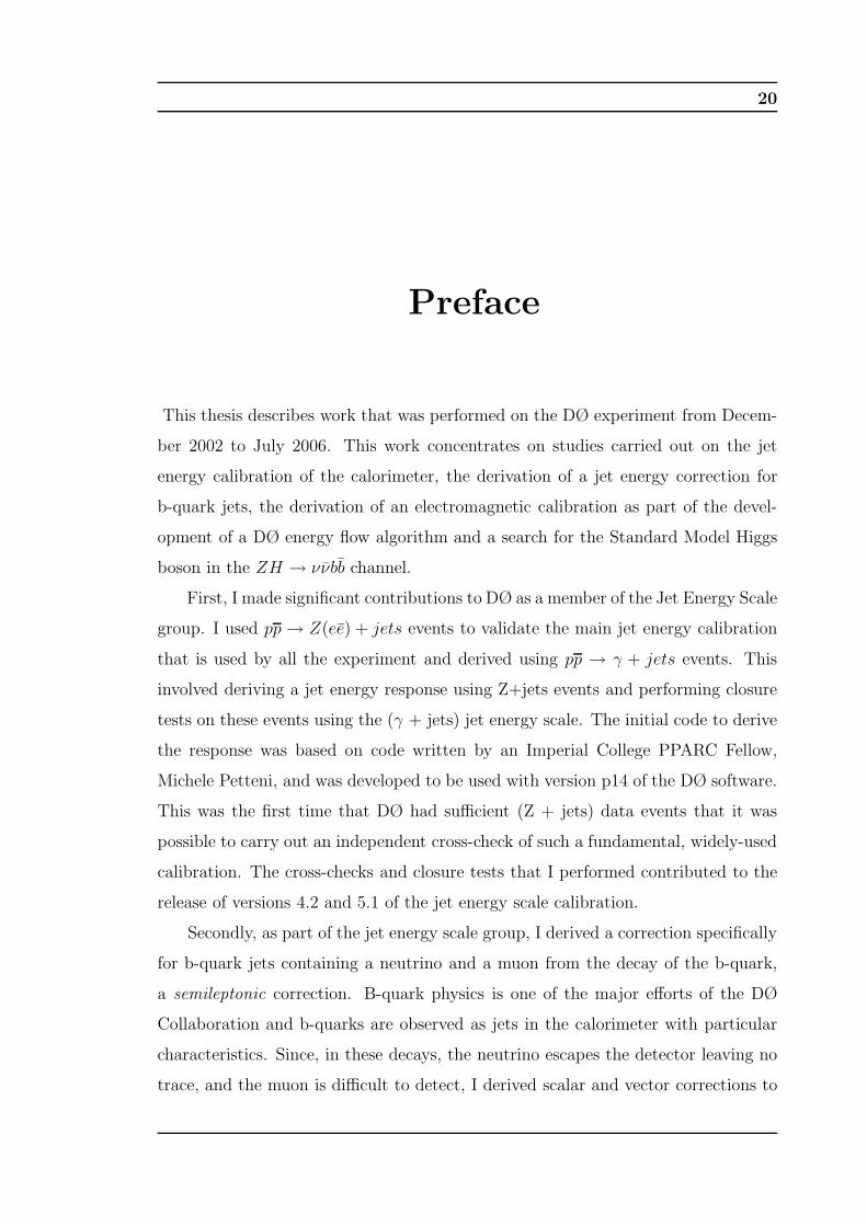
This thesis describes work that was performed on the DØ experiment from Decem-
ber 2002 to July 2006. This work concentrates on studies carried out on the jet
energy calibration of the calorimeter, the derivation of a jet energy correction for
b-quark jets, the derivation of an electromagnetic calibration as part of the devel-
opment of a DØ energy flow algorithm and a search for the Standard Model Higgs
boson in the ZH → ννbb channel.
First, I made significant contributions to DØ as a member of the Jet Energy Scale
group. I used pp → Z(ee) + jets events to validate the main jet energy calibration
that is used by all the experiment and derived using pp → γ + jets events. This
involved deriving a jet energy response using Z+jets events and performing closure
tests on these events using the (γ + jets) jet energy scale. The initial code to derive
the response was based on code written by an Imperial College PPARC Fellow,
Michele Petteni, and was developed to be used with version p14 of the DØ software.
This was the first time that DØ had sufficient (Z + jets) data events that it was
possible to carry out an independent cross-check of such a fundamental, widely-used
calibration. The cross-checks and closure tests that I performed contributed to the
release of versions 4.2 and 5.1 of the jet energy scale calibration.
Secondly, as part of the jet energy scale group, I derived a correction specifically
for b-quark jets containing a neutrino and a muon from the decay of the b-quark,
a semileptonic correction. B-quark physics is one of the major efforts of the DØ
Collaboration and b-quarks are observed as jets in the calorimeter with particular
characteristics. Since, in these decays, the neutrino escapes the detector leaving no
trace, and the muon is difficult to detect, I derived scalar and vector corrections to

Preface 21
compensate for this. The scalar correction formed part of versions 5.1 and 5.3 of
the jet energy scale correction.
Thirdly, my next focus was on deriving a low-energy calibration for the elec-
tromagnetic (EM) calorimeter as part of the energy flow group. To improve the
measurement of low energy particles, DØ developed an algorithm to combine mea-
surements in the tracking system, which are more accurate at low-momentum, and
energy measurements in the calorimeter. My study formed a necessary step in the
development of the energy flow algorithm.
Lastly, as part of the Higgs physics group, I undertook a search for the Standard
Model Higgs in the ZH → ννbb channel using, for the first time, data taken with
the v13 trigger list that included triggers that select on the topography of events
in this channel. My analysis built on the early analysis of this channel using v12
data by Makoto Tomoto. My study, carried out in collaboration with an Michele
Petteni, used advanced techniques to optimise this cuts-based analysis including the
first use of the DØ neural net b-tagging tool developed by Tim Scanlon and Miruna
Anastasoaie.
The thesis is structured as follows:
• Chapter 1 gives a concise account of the Standard Model with a focus on the
relevant areas of Higgs physics;
• Chapter 2 outlines the workings of the Tevatron, the Fermilab proton-antiproton
accelerator, and the DØ detector setup;
• Chapter 3 describes the jet energy response derived using (Z + jets) events,
compares it to the equivalent (γ + jets) response and evaluates closure tests
carried out on (Z + jets) events using the (γ + jets) jet energy correction;
• Chapter 4 gives a description of the derivation of the muonic semileptonic
correction to b-quark jets and details the EM calibration that was calculated
as a component of the development of the energy flow algorithm;
• Chapter 5 details the search for the Standard Model Higgs boson using Run
II data taken using trigger list version 13 at D��O. This includes the process

Preface 22
for selecting candidate events, background simulation and estimation, and the
optimisation of this selection procedure including the use of the neural net
b-tagging tool. The results of this analysis are evaluated and discussed;
• Chapter 6 concludes with a summary and considers the future.
1 The Standard Model and the Higgs Boson 23
Chapter 1
The Standard Model and the
Higgs Boson
1.1 Introduction
From before Democritus first suggested that matter is made of indivisible particles
or atoms [11] in the fourth century B.C, natural philosophers have been search-
ing for a theory that describes how the matter around us is structured and how
it interacts. It was only in the 20th century, when both the mathematical and
technological tools became available, that it was possible to start to probe deep in-
side the atom, eventually revealing the structure of the matter particles (fermions),
and the force particles (bosons) that mediate the interactions. The Standard Model
(SM), for the most part, successfully describes the fundamental particles in terms
of an SU(3)×SU(2)×U(1) gauge theory and has been precisely tested. This chapter
briefly describes the Standard Model and the symmetries upon which it is based,
with a focus on electroweak theory and the Higgs mechanism.
1.2 The Standard Model 24
1.2 The Standard Model
1.3 Matter and its Interactions
Particle families The Universe, at the most basic level that it is currently un-
derstood, is made up of three ‘generations’ or ‘families’ of particles called fermions
which can be subdivided into quarks and leptons. Everyday matter is made from
the lightest generation which includes the electron, and the up and down quarks
that make up the protons and neutrons in nuclei. This first generation also includes
electron neutrinos which are constantly travelling through us, coming mostly from
fusion reactions within the Sun. Each particle within this first generation has its
own distinct properties. There are two heavier ’generations’ which contain particles
in patterns identical to those of the first generation in all ways but their masses.
These are not observed in everyday matter, as they are unstable and so are only
produced in high-energy environments like the Tevatron accelerator, surviving for
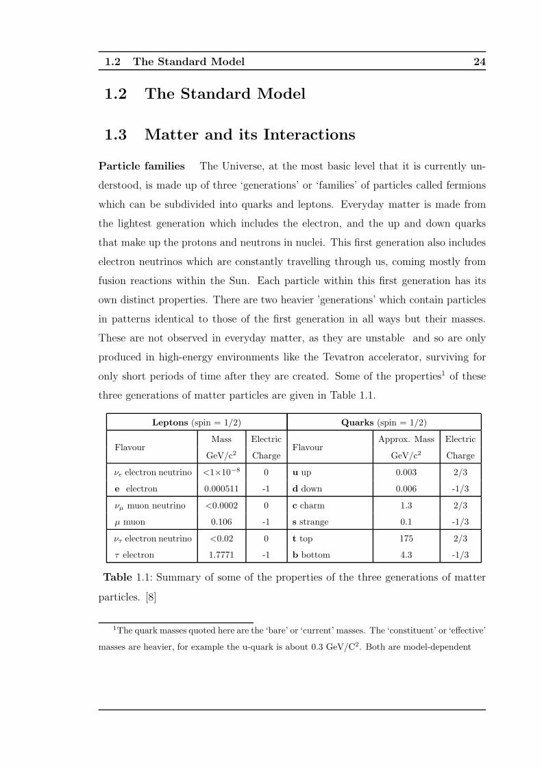
only short periods of time after they are created. Some of the properties1 of these
three generations of matter particles are given in Table 1.1.
Leptons (spin = 1/2) Quarks (spin = 1/2)
FlavourMass Electric
FlavourApprox. Mass Electric
GeV/c2 Charge GeV/c2 Charge
νe electron neutrino <1×10⁻⁸ 0 u up 0.003 2/3
e electron 0.000511 -1 d down 0.006 -1/3
νµ muon neutrino <0.0002 0 c charm 1.3 2/3
µ muon 0.106 -1 s strange 0.1 -1/3
ντ electron neutrino <0.02 0 t top 175 2/3
τ electron 1.7771 -1 b bottom 4.3 -1/3
Table 1.1: Summary of some of the properties of the three generations of matter
particles. [8]
1The quark masses quoted here are the ‘bare’ or ‘current’ masses. The ‘constituent’ or ‘effective’
masses are heavier, for example the u-quark is about 0.3 GeV/C2. Both are model-dependent

1.4 Gauge Theories 25
Particle Interactions These three generations of particles interact via the four
forces, which correspond to the exchange of force carrying bosons: the electromag-
netic force affects all charged particles, the strong binds nuclei together, the weak
force is responsible for some nuclear reactions like β-decay and the gravitational
force. The gravitational force is very weak compared to the other three forces, and
has a negligible effect in particle physics. All these particles and their interactions,
except for gravity, are described in the Standard Model (SM), a good description of
which may be found in many well-respected reviews such as [12] and [13]. Table 1.2
describes some of the properties of these forces.
Property Gravitational Weak Electromagnetic Strong
(Electroweak)
Acts on Mass - Energy Weak Isospin Electric Charge Colour Charge
Particles All Quarks Electrically Quarks
Experiencing Leptons charged Gluons
Particles Mediating Graviton W+,W−, Z0 photon (γ) Gluons
Strength relative to10−41 0.8 1 25
Electromagnetic force
Table 1.2: Summary of some of the properties of the force-mediating particles of
the Standard Model. [8]
1.4 Gauge Theories
Symmetries in nature often conceal fascinating fundamental ideas about physics
that may be described mathematically, that may be used to classify shapes, pat-
terns and other phenomena. An important area of mathematics, group theory2,
can describe the transformations under which an object is symmetric. Symmetries
in physics have important physical consequences summarised in Noether’s theorem
[14]:
2A group is a set of objects that is closed, associative, has an identity element and every
element has an inverse. The U(1) group is a group of all 1×1 unitary matrices.
1.4 Gauge Theories 26
“For any continuous symmetry exhibited by a physical law, there is a
corresponding continuous observable quantity that is conserved.”
The SM is a quantum field theory, described by a Lagrangian comprising terms
composed of fermion and boson fields. The Lagrangian is invariant under certain
transformations, called gauge transformations which may be simply thought of as
rotations. When a gauge transformation is identically performed at every space-time
point and the Lagrangian remains unchanged then it is said to be globally invariant.
However, gauge theory is based upon the idea that the Lagrangian is also invariant
under local transformations3. The gauge theory class of mathematics was developed
in 1954 by Yang and Mills [15] and it is this type of mathematics that forms the basis
of the Standard Model, providing a framework with which to describe the quantum
field theories of the strong, weak and electromagnetic forces.
The idea of gauge invariance of the SM Lagrangian may be most easily under-
stood by first considering a simple global gauge transformation applied to the Dirac
Lagrangian, L , which describes free fermion fields:
LD = Ψ(iγµ∂µ −m)Ψ (1.1)
where Ψ and Ψ are the fermion field and its conjugate respectively, γµ are the 4×4
gamma matrices and m is the fermion mass. If we now transform the field with the
global gauge transformation4, Ψ → e−iωΨ, Ψ → eiωΨ, where ω is real and constant
and e−iω is the U(1) group, then LD remains unchanged. This particular manifest
invariance can be observed in current conservation or the conservation of electric
charge.
The Yang-Mills gauge theory extended this idea of a global symmetry by requir-
ing that Lagrangians must also possess local symmetries. A global transformation
means that all points in space-time (x) know about the transformation instantly and
it does not take into account that the signal requires time to travel. A more ‘realis-
tic’ requirement, that also leads to more interesting physics, is to require that gauge
3A local transformation is a symmetry that could be defined arbitrarily from one position to
the next and is dependent on space-time coordinates.4It is called a global transformation because it is not dependent on space-time coordinates.

1.4 Gauge Theories 27
invariance really is a basic property of nature so requiring that the Lagrangian is
invariant under local transformations. This means that the transformation depends
on the space-time point and is now written as Ψ → Ψ′ = eiqω(x)Ψ(x). Substituting
this into 1.1 leads to an extra term, δL in the Lagrangian :
δL = Ψ(x)γµ[∂µω(x)]ω(x)Ψ(x) (1.2)
This must be compensated for if the Lagrangian is to be unchanged. In this case,
this is done by introducing the electromagnetic force in the form of a real vector
gauge field, Aµ, to represent photons with which the fermion field can interact. Aµ
transforms as:
Aµ → A′
µ = Aµ +1
e∂µω(x) (1.3)
and the term eΨγµAµΨ represents the interactions of the gauge field with the fermion
field. The Lagrangian becomes:
L = Ψ(iγµ(∂µ + ieAµ) −m)Ψ (1.4)
where e is the fermion charge. We need to include a kinetic energy (K.E.) term for
the photon field, which itself must be invariant. So we use the K.E. term:
−1
4FµνF
µν (1.5)
where Fµν = [JµAν ]− [JνAµ]. Thus we arrive at the Lagrangian density for quantum
electrodynamics, QED:
L = −1
4FµνF
µν + Ψ(iγµ(∂µ + ieAµ) −m)Ψ (1.6)
It is not possible to add any mass terms of the form M2AµAµ as is not gauge
invariant. At this point, it is convenient to group the partial derivative and the
term explicitly containing the gauge field to define the covariant derivative, Dµ:
Dµ ≡ ∂µ + ieAµ (1.7)
so that 1.6 becomes:
LQED = −1
4FµνF
µν + Ψ(iγµDµ −m)Ψ (1.8)
1.4 Gauge Theories 28
It is this covariant derivative that groups together the interesting terms that describe
the interactions of the particle fields and gauge fields, this becoming more apparent
when we generalise this idea of symmetry in the next section. The covariant deriva-
tive has the property that it transforms in the same way as the particle fields under
gauge transformations. Furthermore, the field strength tensor may be expressed in
terms of Dµ,
Fµν = − i
g[Dµ, Dν ] (1.9)
where g is the coupling constant which determines the strength of an interaction. In
the case of the U(1) symmetry that represents QED, g = e, the electronic charge.
So, the whole Lagrangian density has been derived from the requirements of local
gauge invariance of the U(I) gauge symmetry and the requirements of QFT.
1.4.1 Non-Abelian Gauge Transformations
In a similar fashion to the U(1) symmetry described in the previous section, gauge
transformations may be applied to the SU(2) symmetry group which describes the
weak force, and the SU(3) group of QCD. A Lagrangian may be constructed for
a general gauge theory by considering the arbitrary transformation, SU(n), repre-
sented by the matrices e−ωaT
a
where there are n2-1 gauge fields that interact with the
particles (unlike the singlets in the U(1) transformation) that transform as follows:
Ψi → Ψ′
i = (e−iωa
Ta)jiΨj (1.10)
Substituting the transformation in Equation 1.10 into the appropriate Lagrangian,
as before, leads to extra terms. As in the Abelian case, these must again be com-
pensated for by the addition of vector gauge fields, Waµ. So the covariant derivative
becomes:
Dµ = (∂µI + igTaW aµ ) (1.11)
where I are the unit matrices of order n. The Lagrangian becomes, after adding in
the K.E. term, as before:
L = Ψi(iγµDµ −mI)jiΨj −
1
4F a
µνFµνa (1.12)
1.5 Electroweak Theory 29
Similarly, the K.E. term is still constructed from the field strengths F aµν as in Equa-
tion 1.9, but Fµν is in a more complex form since the generators of the group do not
all commute:
F aµν = ∂νA
aµ − ∂µA
aν − gfabcAb
νAcν (1.13)
The last term here, when substituted into the Lagrangian, leads to terms such as
gfabc(∂µAaν)A
bµA
cν and 1
4g2(fabcfabeAb
µ)AcνA
dµA
eν which arise because of the properties
of non-Abelian transformations and imply that these gauge bosons interact with
each other. As before, a mass term is still forbidden as it is not gauge invariant. In
the case of the SU(2) weak force, this leads to weak isospin doublets of particles,
and three vector gauge bosons. Weak isospin is the equivalent of electric charge for
the weak force; see section 1.5 for more details. For the strong force with its SU(3)
symmetry, there are then eight gauge bosons (gluons) with six colour triplets of the
quarks, where colour is the QCD equivalent of the electric charge in QED.
1.5 Electroweak Theory
Problems with the separate SU(2) and U(1) descriptions of the weak and electro-
magnetic (EM) forces led Glashow, Weinberg and Salam (GSW) to propose inde-
pendently between 1961 and 1967 a theory that unified these interactions into one
electroweak theory [16], [17], [18]. This unification was suggested before the W and
Z bosons had been discovered, and their theory successfully predicted the existence
of the neutral weak current involving the Z0 boson. GSW had noted the similari-
ties of the weak charged current and EM interactions, and that weak interactions
only involve the left-handed particles. They proposed a theory of SU(2)L⊗U(1)Y
symmetry which interacts with the left-handed and right-handed components of the
fermion fields separately.
The weak interaction is described by the SU(2)L symmetry with gauge bosons
Waµ (a=1,2,3), which lead to two charged bosons and one neutral one. However,
from experimental observations such as charged pion decay, we know that the cou-
pling strengths of weak interactions are different for left-handed and right-handed
particles. In fact, the charged bosons only couple to left-handed fermions and
1.5 Electroweak Theory 30
right-handed anti-fermions, and no right-handed neutrinos have been observed. So
the fermion field, Ψ, is split into its left and right-handed components, Ψ = ψL +ψR,
so that each may be treated separately. The fermion field is now made up of left-
handed weak isospin doublets, ψiL, whose weak ’charge’, isospin, takes the value
T=1/2, using the notation of the previous section and the right-handed fermions
are isosinglets, ψiR, with T=0:
ψiL =
νe
e
L
;
νµ
µ
L
;
ντ
τ
L
;
u
d
L
;
c
s
L
;
t
b
L
(1.14)
ψiR = eR ; µR ; τR ; uR ; dR ; cR ; sR; tR ; bR (1.15)
T is the weak equivalent to the EM charge, so that when T=0, there is no weak
interaction. No right-handed neutrinos are needed in this model. Recent results
show that neutrinos oscillate [19], [20], implying a non-zero neutrino mass. Exten-
sions to the SM, including right-handed neutrinos have been postulated [21]. The
U(1) symmetry of the EM interactions is included indirectly by adding a field, Bµ
with a U(1)Y symmetry to the weak Lagrangian where the generator, Y, is not the
electric charge but hypercharge. The Bµ field will interact with both the left-handed
and right-handed quarks and leptons. This then mixes with the W0 field to form
the Zµ and Aµ fields. The fermion doublets are assigned a hypercharge, Y=-1 and
the singlets, Y=-2. Taking the two symmetries together, left-handed components
transform as:
ψL → ψ′L = eiα(x).T+iβ(x)YψL (1.16)
and the right-handed components transform as
ψR → ψ′R = eiβ(x)YψR (1.17)
The interaction terms in the Lagrangian become:
Linteraction = ψi(iγµ(∂µI + igTaW aµ + i′
Y
2Bµ
︸ ︷︷ ︸
covariant derivative, Dµ
))jiΨj (1.18)
The EM interaction is hidden in this Lagrangian as a mixing between W3µ and Bµ
that leads to the physically identifiable Z0 and γ bosons via the weak mixing angle,
1.5 Electroweak Theory 31
θW . In understanding this mixing, a third quantum number, the third component
of the weak isospin, T3, is used where the T=12
doublets have T3=+12
for the more
positive particle in the doublet, and T3=−12
for the more negative particle. The
right-handed singlets have T3=0.
Aµ = Bµ cos θW +W µ,3 sin θW (1.19)
Zµ = −Bµ sin θW +W µ,3 cos θW (1.20)
The W1µ and W2
µ fields and their generators are also mixed to form the observed W±
bosons:
W±µ =
1√2(W 1
µ ± iW 2µ ) and T±
µ =1√2(T1
µ ∓ iT2µ) (1.21)
Substituting the inverses of Equations 1.19, 1.20 and 1.21 into the electroweak
Lagrangian, and leaving out the K.E. terms to focus on the interaction terms, after
grouping the W±, Aµ and Zµ fields, the interaction Lagrangian becomes:
Linteraction = Ψγµg(T+µWµ + T−
µWµ)Ψ (1.22)
+ Ψγµ(gT3 cos θW − g′Y
2sin θW )ZµΨ (1.23)
+ Ψγµ(gT3 sin θW − g′Y
2cos θW )AµΨ (1.24)
The charged current weak interactions are described by the first term and only
involve the left-handed components of Ψ since T=0 for the right-handed components.
The second term describes the observed weak neutral currents that may involve
either the right-handed or the left-handed particles. This term may be expanded to
show this explicitly:
ψLγµ(gT3 cos θW − g′Y
2sin θW )ZµψL + ψRγ
µg′Y
2sin θWZµψR (1.25)
The third term describes the EM interactions and the generator of the U(1)EM
symmetry, Q, may be identified as Q=T3 + Y
2. The EM interaction term is of the
form ΨeγµAµΨ as identified in the QED Lagrangian in Equation 1.6. Comparing
this to the last term allows the constraint
g sin θW = g′ cos θW = e (1.26)

1.6 The Higgs Mechanism 32
to be placed on g,g’ and θW .
There is, however, a key problem in that the SU(2)L⊗U(1)Y symmetry, in itself,
does not explain why the two neutral gauge fields, W3µ and Bµ, mix or indeed why
the W± and Z0 bosons have mass but the photon remains massless. Neither does
it explain how the fermions acquire mass. Earlier, it was mass terms of the form
m2WµWµ that were not allowed in the Lagrangian as they are not gauge-invariant,
but now mass terms of the fermion fields of the form mΨΨ cannot be included
either. These mix the left-handed and right-handed states which undergo different
gauge transformations as in Equations 1.16 and 1.17, so the resultant mass term is
no longer invariant.
1.6 The Higgs Mechanism
The Higgs mechanism spontaneously breaks the electroweak symmetry down to a
U(1) symmetry, introducing the masses of the W and Z bosons, while allowing the
photon to remain massless [22], [23]. It allows the Lagrangian to remain invariant
under the U(1) symmetry group, but the vacuum state is not and has a non-zero
vacuum expectation value. The Higgs field is itself gauge invariant, and an expansion
around its vacuum expectation value produces the couplings to the gauge boson and
fermion fields (Yukawa couplings). In this way, mass terms for the gauge fields, the
gauge bosons and even for the Higgs field itself appear. The mechanism then predicts
the existence of the Higgs boson and all of its properties except its mass; to date
the Higgs boson has not been observed.
Considering the simplest case of an Abelian U(1) gauge theory with a scalar
field, Φ, and the addition of a scalar potential V (Φ), the Lagrangian may be written
as:
L = (DµΦ)∗(DµΦ) − 1
4FµνF
µν − V (Φ) (1.27)
where Dµ ≡ ∂µ + ieAµ. The potential V (Φ) is given by
V (Φ) = µ2Φ∗Φ + λ|Φ∗Φ|2 (1.28)
and can be likened to the U term for potential energy in the classical Lagrangian
L = T − U . As long as V (Φ) is composed of terms of the form Φ∗Φ then the
1.6 The Higgs Mechanism 33
Lagrangian will remain gauge invariant under the U(1) transformation Φ → e−iω(x)Φ
and the form of V chosen here is the minimum required to retain the gauge symmetry
such that the theory remains renormalisable. Assuming λ > 0, we will consider
the two cases where µ2 is greater than or less than zero. For µ2 > 0, the potential
V has the shape shown on the left in Figure 1.1; however, for µ2 < 0, the potential
takes on the form on the right in Figure 1.1. In the latter case, the system is not in
its ground state at Φ = 0, but has a vacuum expectation value, v =√
µ2/λ. The
ground state is now at Φ = eiθv/√
2 where θ can take any value from 0 to 2π. This
means that there are infinitely many ground states and the system is still symmetric.
The spontaneous symmetry breaking occurs when a choice is made as to which θ
represents the true vacuum. Once this decision has been taken, the symmetry is
broken. Expanding Φ around its expectation value gives
Φ(x) =1√2(v + H + iφ) =
1√2(v + h)ei θ(x)
v (1.29)
where h will correspond to the physical Higgs field. It is possible to choose the U(1)
gauge transformation so that φ disappears:
Aµ → Aµ +1
ev∂µθ (1.30)
and this is called the Unitarity gauge. Substituting Equation 1.29 into 1.28 gives:
V (Φ) = µ2H2 + µ√λH2 +
λ
4(H4 + 2H2) +
µ4
4λ(1.31)
Then substituting 1.31 into 1.27 leads to:
L =1
2(∂µh)
2 + µ2h2 +1
2e2v2A2
µ +µ4
4λ− λvh3 − λ
4h4 +
1
2e2A2
µh−1
4FµνF
µν (1.32)
From this, a scalar field, h, of mass√
−2µ2 and a vector field (Aµ) of mass ev,
may be identified. There are also interaction terms which describe the three and
four-point interactions of the Higgs field with the vector field (‘hhh’, ‘hhhh’, ‘AAhh’
and ‘AAh’). There is also the kinetic energy term as seen before. This is the Higgs
mechanism and h is the Higgs boson. In this case, used as a simple example of the
Higgs mechanism, a mass has been introduced for the photon but gauge invariance
is preserved.
1.6 The Higgs Mechanism 34
Figure 1.1: The shape of the potential V (Φ) for different values of µ [1].
This mechanism can be extended to the SU(2)⊗U(1) electroweak symmetry by
considering a complex doublet of four scalar fields:
Φ =
Ψ+
Ψ0
=1√2
ψ1 + iψ2
ψ3 + iψ4
(1.33)
This form of Ψ was the one originally made by Weinberg in 1967 and is called the
Weinberg-Salam model. To generate the gauge boson masses, the same Higgs po-
tential, V (Ψ) is used with Ψ0, the vacuum expectation value where ψ1 = ψ2 = ψ4 = 0
and ψ23 = −µ2/λ = v ,
ψ0 ≡1√2
0
v
(1.34)
This has Y=1, T=1/2 and T3=-1/2. The choice of ψ0 does break both the SU(2)L
and U(1)Y symmetries, but ψ0 is neutral, i.e. Q=0, so the U(1)EM symmetry with
generator Q (=T3 + Y2) is unbroken. Thus the vacuum remains invariant under
U(1)EM transformations and the photon is massless. All of the three other combi-
nations of the four electroweak generators break the symmetry resulting in masses
for the other gauge bosons. Again, examining the covariant derivative and the ki-
netic term in the EW Lagrangian will give us information about the interactions
with the Higgs field and how the masses of the gauge bosons arise:
Dµ = ∂µ + igWaµT
a + ig′Y
2Bµ (1.35)

1.6 The Higgs Mechanism 35
Expanding Ψ around its vacuum expectation value using the unitarity gauge gives:
ψ0 ≡1√2
0
v +H(x)
(1.36)
with H(x) real. Then again using the unitary gauge and with the substitution
T± = (T 1 ± iT 2)/√
2 and W± = (W 1 ± iW 2)/√
2, the kinetic term, (DµΨ)∗(DµΨ)
becomes:
(DµΨ)∗(DµΨ) =1
2(∂µH)2 +
g
4(v +H)2W+µW−
µ +1
8(v +H)(gW 3
µ − g′Bµ)2 (1.37)
Once this covariant derivative has been substituted into the Lagrangian as before and
the transformation has been made from W 3 and B to Z and A, then the Lagrangian
becomes:
L =1
2(∂µH)2+
1
4g2(v+H)2+
1
8(g2+g′2)(v+H)2ZµZ
µ− 1
4µ2v2+µ2H2−λvH3−λ
4H4
(1.38)
The terms involving v are the mass terms and those involving H describe the in-
teractions of the Wa and B gauge fields with the Higgs field. The mass of the W
boson can thus be identified as
MW =1
2gv (1.39)
The mass of the Z boson is
MZ =1
2
gv
cos θW(1.40)
It can be seen that the ratio of the squares of the W and Z masses, ρ cos2 θW , is a
prediction of the Standard Model:
ρ =M2
W
M2Z cos2 θW
(1.41)
where ρ = 1 in the Standard Model.
Although mass terms of the form mψψ were excluded by gauge invariance in
the Lagrangian, the same Higgs doublet which generates the W and Z masses can
also generate the fermion masses. While an explicit mass term would mix the left-
handed and right-handed fermions and is not allowed, an interaction between the
left-handed doublet, the Higgs doublet and the right-handed singlet is allowed. Such

1.7 Current Limits on the Higgs Mass 36
terms, called Yukawa interactions, will generate mass terms for the fermions of the
form:
Gl[φLΨφR + φRΨφL] (1.42)
where Gl is the Yukawa coupling for leptons. For example, for electrons, this will
generate a mass me = Gev/√
2 and a coupling to the Higgs field proportional to its
mass. This will also leave the neutrino massless. The three generations of leptons
are added to this model as copies of each other, with different Yukawa couplings so
that the masses of the muons and the tau-leptons are correct. Slightly more complex
Yukawa terms are needed when including the quark doublets and singlets, to ensure
that both the ’up’ and ’down’ types acquire mass. For further detail see, amongst
others, [12] and [24].
1.7 Current Limits on the Higgs Mass
Once the mass of the Higgs is known, all the parameters of the SM Higgs may be
calculated, as the mass is the only free parameter. Currently the Higgs mass is not
known, but it is possible to put upper and lower bounds on its value from theory,
and experimental searches and measurements.
1.7.1 Limits from Theory
Unitarity requirements in WW scattering require that there is an upper bound of
1.2 TeV [25]. Running of the Higgs coupling, λ, with the energy scale, Λ, places
tighter limits on the Higgs mass. These theoretical bounds on the Higgs mass with
Λ are shown in Figure 1.2. The upper and lower limits are set by requiring that Λ
has sensible values and that the Higgs potential minimum is maintained. The upper
limit requires that λ(Λ) <∞ from the idea that radiative loop corrections involving
the Higgs self-interactions affect λ and this limit can be expressed as a constraint on
the Higgs mass. At the lower limit, λ(Λ) > 1 as this is the requirement for vacuum
stability . Assuming that SM Higgs physics is valid from the Planck mass up to
Λ ∼ 1019GeV, then the Higgs mass will have to lie in the range 135GeV to 180GeV.
1.7 Current Limits on the Higgs Mass 37
Figure 1.2: Upper and lower theoretical bounds on the Standard Model Higgs mass
as a function of the energy scale. [2]
1.7.2 Limits from Indirect Methods
Many electroweak parameters are sensitive to the Higgs mass via higher order loop
corrections. For example, predictions of the masses of the W boson and the top
quark are related to the Higgs mass via these higher order corrections, leading to a
logarithmic dependence of the Higgs mass on the W boson and top quark masses.
This dependence is illustrated in Figure 1.3. The same study combined 18 separate
input measurements including the width of the W boson and measurements from
high-Q2 interactions to obtain the most stringent constraint on the Higgs mass.
Figure 1.4 shows the χ2(mH) = χ2min(mH ) − χ2
min curve [3] as a function of Higgs
mass. The preferred value for MH , corresponding to the minimum of the parabola
given by the black line, is 85 GeV, with an experimental uncertainty of +39GeV
and -28GeV (at 68% C.L.) The 95% C.L. upper limit on MH <199GeV.
1.7 Current Limits on the Higgs Mass 38
80.3
80.4
80.5
150 175 200
mH [GeV]114 300 1000
mt [GeV]
mW
[G
eV]
68% CL
∆α
LEP1, SLD data
LEP2 (prel.), pp− data
Figure 1.3: Contour curves of 68% probability in the (mt,mW ) plane. The shaded
band shows the SM prediction for the Higgs mass. [3]
1.7.3 Limits from Direct Methods
Direct searches for the Higgs have also been carried out using the production mech-
anisms and decay modes that combine to give the greatest sensitivity at that partic-
ular collider. The most stringent limits on the Higgs mass come from the measure-
ments made at LEP2 [26]. The primary production mechanism expected at LEP
was the Higgs-strahlung process, e+e− → HZ, with small contributions from W
and Z boson fusion processes . For masses around 115GeV, the Higgs is expected
to decay mainly into bb pairs, with searches including all possible decay modes for
the Z combined. The LEP collaborations performed a search on 2465pb−1 of data,
from e+e−collisions between 189GeV and 209GeV, and have imposed a lower bound
1.7 Current Limits on the Higgs Mass 39
0
1
2
3
4
5
6
10030 300
mH [GeV]
∆χ2
Excluded
∆αhad =∆α(5)
0.02758±0.00035
0.02749±0.00012
incl. low Q2 data
Theory uncertainty
Figure 1.4: χ2(mH) = χ2min(mH ) − χ2
min as a function of mH . The line is the result
of the fit using 18 electroweak parameters. [3]
of 114.4GeV on the Higgs mass at the 95% C.L. The likelihood analysis shows some
preference for a Higgs boson with a mass of 115.6GeV, with the probability for the
background to generate the observed effect of 3.4%. The production mechanisms and
decay modes of the light SM Higgs boson are discussed in more detail in Chapter 5.
Prior to LEP2, Higgs searches were also carried out by the CDF collaboration
at the Tevatron during Run I [27], though the results are weaker than those of
the LEP2 search. The Higgs was searched for in associated production with a
W or Z boson, where the Higgs decays to a bb pair, in approximately 110 pb−1
data taken at a centre-of-mass energy of 1.8 TeV. CDF measured upper limits on
σ(pb→V H)×BR(H → bb) which are substantially higher than those predicted in the
Standard Model. With the higher energy collider and the larger dataset available,
Higgs searches have returned to the physics agenda at the Tevatron, with ZH being
1.8 Conclusions 40
one of the most sensitive production mechanisms due to its large production cross-
section and the large branching ratio of Z → νν.
1.8 Conclusions
The Standard Model currently well-describes the strong, electromagnetic and weak
forces and the fundamental particles, the leptons and the quarks, that we observe in
high energy physics experiments. It is based on a SU(3)⊗SU(2)L⊗U(1)Y symmetry,
with the weak and EM forces unified in the electroweak theory. This symmetry
itself does not explain the masses of the W and Z quarks, nor why the symmetry is
broken such that the photon remains massless.
To generate mass, the Higgs mechanism is introduced whereby the SU(2)⊗U(1)Y
symmetry is spontaneously broken down to the U(1)EM symmetry. This mechanism
generates the masses of the gauge bosons and the fermions, but it cannot predict
their masses nor the mass of the Higgs boson itself, all of these being just parameters
of the theory. Many observables within the electroweak sector are sensitive to the
Higgs mass (MH), and by measuring these accurately, constraints may be placed
on MH . The predicted Higgs couplings to the gauge bosons and the fermions are
proportional to their masses. Since the Higgs is massive, it is only high-energy
facilities like the Tevatron and the LHC that will be able to discover the Higgs if
it exists in this form. Theory suggests that the Higgs mass is probably between
135GeV and 180GeV [2], but combined results from indirect and direct searches
compellingly indicate that the Higgs has a mass greater than 114.4GeV from direct
searches. Indirect evidence points to MH <200GeV.
At the Tevatron, for Higgs with a mass around 130 GeV, the most promising
production mechanism is qq → V H (V is Z/W), and where this is followed by the
decay of the Higgs to a bb pair and the leptonic decay of V. The final states with the
most potential are lνbb, ννbb, llbb, and qqbb with the main backgrounds Wbb and
WZ processes. This means that the b-tagging capability, the jet energy resolution,
and the E/T resolution and coverage are the key elements for good discrimination of
any possible signal.
2 Experimental Apparatus 41
Chapter 2
Experimental Apparatus
The Tevatron is the highest energy collider (proton-antiproton, pp ) currently in
operation. It runs with a centre of mass energy of√s=1.96TeV at the Fermi Na-
tional Accelerator Laboratory (Fermilab) near Chicago. DØ and CDF are the two
large, general-purpose collision-detector experiments that are part of a wide exper-
imental programme that also includes research into neutron physics and medical
physics amongst other things. In this chapter, an outline is given of the accelerator
complex needed to reach this centre of mass energy, a brief description of the DØ de-
tector apparatus is presented, and an explanation of how particles interact with the
detector is given. The main focus of the DØ experiment is Higgs physics, b-quark
physics, and high pT phenomena1. The running of the detector is split into two runs:
Run I and Run II. The original detector [28] has been upgraded several times since
1992. During Run I, which lasted from 1992 - 1996, significant results included the
discovery of the top quark [29], and the measurement of its mass [30],[31]. Run II
can be divided into Run IIa and Run IIb; the split was defined by further upgrades
to enable the detector to cope with the increased luminosity of the Tevatron. The
current DØ detector is described in detail in [32] and the Run IIa/b upgrades are
described in [33]. This thesis focuses on studies with the Run IIa detector only,
which started in March 2001, after extensive upgrades to the DØ detector.
1High pT phenomena: these include top quark physics, W physics and QCD measurements.
2.1 The Tevatron 42
2.1 The Tevatron
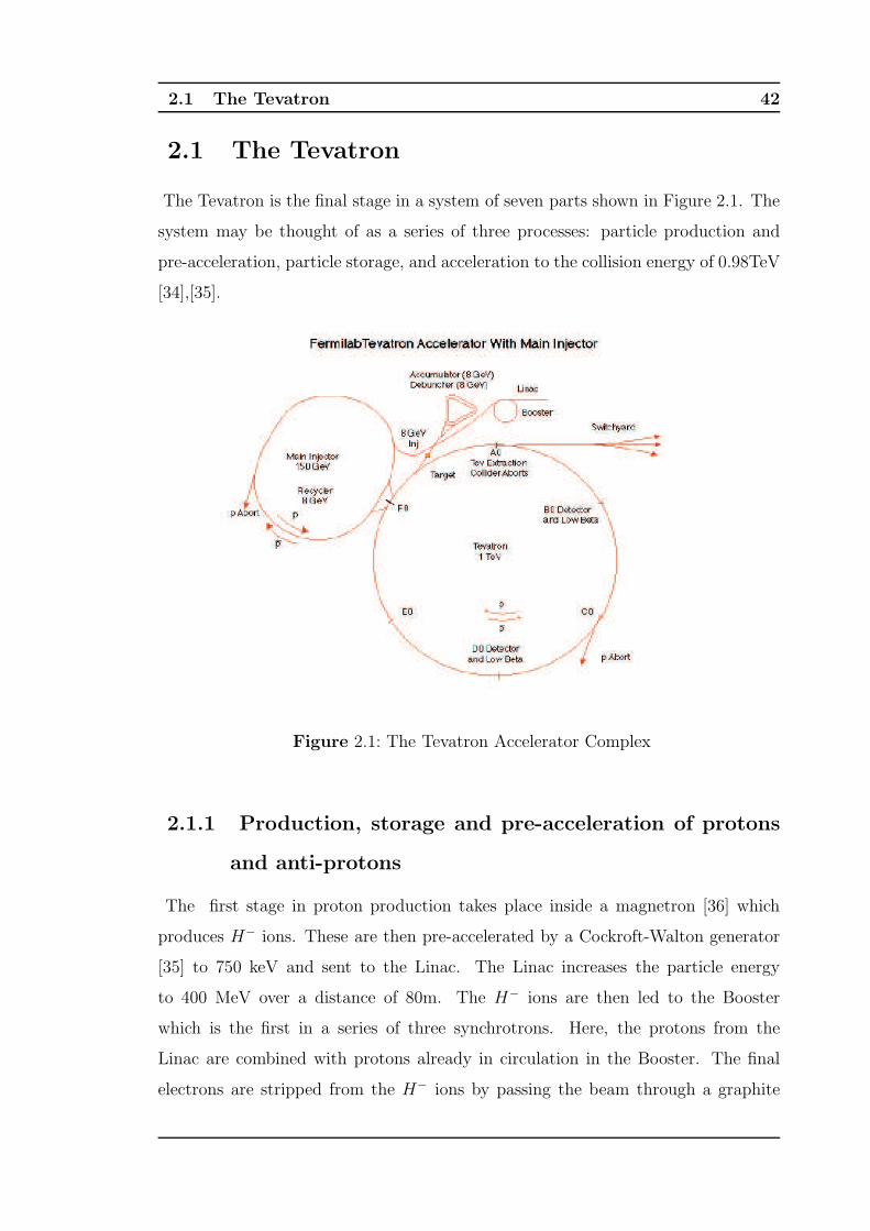
The Tevatron is the final stage in a system of seven parts shown in Figure 2.1. The
system may be thought of as a series of three processes: particle production and
pre-acceleration, particle storage, and acceleration to the collision energy of 0.98TeV
[34],[35].
Figure 2.1: The Tevatron Accelerator Complex
2.1.1 Production, storage and pre-acceleration of protons
and anti-protons
The first stage in proton production takes place inside a magnetron [36] which
produces H− ions. These are then pre-accelerated by a Cockroft-Walton generator
[35] to 750 keV and sent to the Linac. The Linac increases the particle energy
to 400 MeV over a distance of 80m. The H− ions are then led to the Booster
which is the first in a series of three synchrotrons. Here, the protons from the
Linac are combined with protons already in circulation in the Booster. The final
electrons are stripped from the H− ions by passing the beam through a graphite
2.1 The Tevatron 43
sheet. Once sufficient protons are accumulated in the Booster, they are sent to the
main injector to be further accelerated. Some of the accelerated protons from the
main injector are used in the antiproton system which comprises the target station,
the debuncher and the accumulator, shown in Figure 2.1. These protons from the
main injector are directed onto a Nickel target at 120GeV, producing a shower of
secondary particles, some of which are p. A lithium lens is used to focus the wide
beam produced and to remove positively charged particles. Stochastic cooling2 is
then used to reduce the momentum and position spread of the antiprotons in the
debuncher and accumulator.
It is very difficult to produce antiprotons and approximately 20 antiprotons are
produced for every million protons used in this process. The antiprotons are stored
in the accumulator until a sufficient number have been collected to transfer to the
main injector and this process, known as a store, takes many hours.
2.1.2 Particle Acceleration
The main injector is a circular synchrotron of diameter 1km. It accelerates the
protons and antiprotons from the booster and the antiproton source to 150GeV and
injects them into the Tevatron. The Tevatron is the final synchrotron in which the
protons and antiprotons are accelerated in opposite directions in the same beam
pipe. It uses 774 dipole and 216 quadrupole superconducting magnets with fields
up to 4T at the temperature of liquid Helium. The Tevatron has a diameter of
2km and increases the energy of the particles to 0.98 TeV. From Figure 2.1, it can
be seen that protons travel clockwise around the ring from BØ (CDF) towards DØ
(and around and out towards the fixed target experiments via the switchyard). The
protons and anti-protons (pp ) are grouped together in bunches, and the Tevatron
creates 36 bunches approximately 50 cm long, of both protons and antiprotons from
each store, separating them into three groups of ‘super bunches’. The bunches are
2Stochastic cooling: technique to reduce momentum spread in a storage ring for charged
particles. Fluctuations in the position of the bunches are detected and a correction (a ”steering
pulse” or ”kick”) with the opposite sign is applied. Stochastic refers to the fact that usually not
all particles can be corrected at once; they are cooled down in multiple steps. [37]
2.2 The DØ Detector 44
made to collide at two points on the Tevatron ring with a time spacing between each
collision of 396ns; one of the points is labelled DØ , hence the experiment’s name.
2.1.3 Tevatron Performance
It is anticipated that the Tevatron will continue running, producing good physics,
until a little while after the LHC at CERN comes online in 2007, when Run II
will end. The total Run IIa integrated luminosity, from 19th April 2002 to 23 May
2006, as recorded by DØ was 1.18fb−1 . Some of the characteristics of Run II are
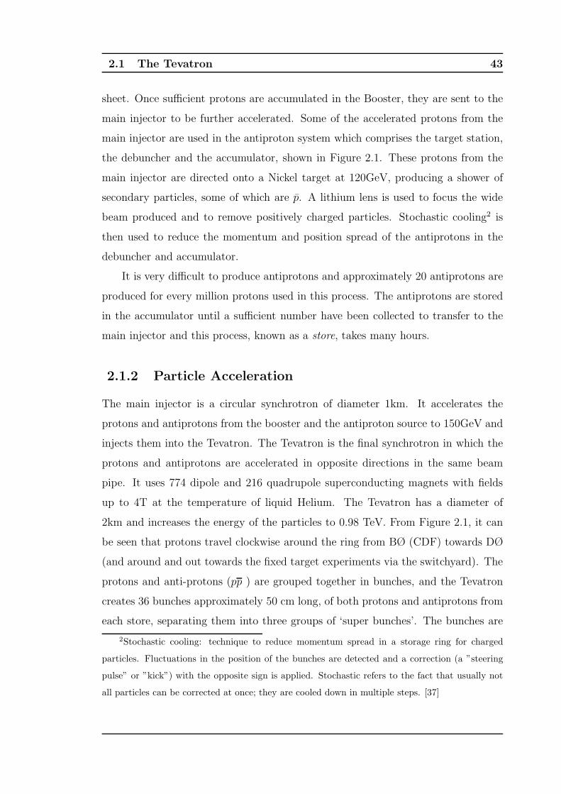
summarised in Table 2.1.
Run II at the Tevatron was originally planned to deliver 2fb−1 but studies of the
physics potential in 2000 and 2003, most notably potential for finding evidence of
the Higgs boson, led to a revised goal of 8fb−1. The Tevatron underwent extensive
upgrades, to gradually increase its peak luminosity to 2 × 1032cm−2s−1, more than
four times the peak luminosity in Run I, and to decrease the bunch spacing from
396ns to 132ns. The current integrated luminosity has already exceeded the design
specifications and it is anticipated that the integrated luminosity to be delivered
will be 4.4fb−1 and 8.8fb−1 over the whole of Run II; Figure 2.2 shows the projected
integrated luminosity over the next few years.
Run II
Centre of mass energy 1.96TeV
Bunch Spacing 396ns
Number of p and p bunches 36
Number of protons per bunch 2.7×10¹¹
Number of antiprotons per bunch 4.2×10¹⁰
Base integrated luminosity 4.4fb−1
Design integrated luminosity 8.8fb−1
Table 2.1: Some key operating characteristics of the Tevatron for Run II
2.2 The DØ Detector
The DØ detector is multi-purpose and constructed like the layers of an onion
around the interaction point. It can measure precisely the kinematic properties of
2.2 The DØ Detector 45
0
1
2
3
4
5
6
7
8
9
10
9/29/03 9/29/04 9/30/05 10/1/06 10/2/07 10/2/08 10/3/09
Start of Fiscal Year
Inte
gra
ted
Lu
min
osi
ty(f
b-1
)Design Projection
Base Projection
Design Base
Figure 2.2: Base and design projected integrated luminosity from the Tevatron up
to 2009 [4]
the particles passing through it by examining their positions and energies. The
detector comprises three major subsystems: at the centre there is a tracking system
that includes a 2T solenoid, around this there is a uranium/liquid argon calorimeter,
and then surrounding this there is a muon system with a toroid magnet to measure
the momenta of muons. Figure 2.3 shows the layout of the detector and these
subsystems, the following subsections describe the detector coordinate system and
these detector subsystems in more detail. Full details can be found in [32].
2.2.1 The Detector Coordinate System and Units
Both polar and Cartesian coordinates are used to describe particles within the
detector. These two sets of coordinates are referred to in two different ways, the
first being physics coordinates where the origin is set at the point of interaction, and
the second is detector coordinates where the origin is set to the centre of the DØ
detector. All momenta and energies are given in GeV.
Cartesian A right-handed system is used with the z-axis increasing along the
proton beam (south). The origin of coordinates is the centre of the detector, with
2.2 The DØ Detector 46
Figure 2.3: The DØ detector
y increasing with height. Positive x points outwards from the centre of the ring
(East). Distances in the detector are usually measured in cm.
Polar These are used interchangeably with the Cartesian coordinates, and the
transformations are as follows:
r =√
(x2 + y2)
φ = arctan y/x
θ = arccos z/√
(x2 + y2 + z2)
where:
• r is the perpendicular distance from the z-axis.
• The azimuthal angle, φ, is measured in radians from 0 to 2π, with φ = 0 for
x > 0, y = 0 and 0 < φ < π for y > 0.
2.2 The DØ Detector 47
• θ is measured in radians from 0 to π, with θ = 0 for x = y = 0 and z > 0,
θ = π for x = y = 0 and z < 0.
Pseudo-rapidity A quantity called pseudo-rapidity (η) is frequently used instead
of θ: η = − ln tan θ/2. Positive η points South. This is derived from the rapidity,
which is Lorentz invariant, given by y = 12[ln(E + pz)/(E − pz)] where the particle
masses are zero, i.e. η ≡ y if m = 0 (≡ β = 1). This is an appropriate transforma-
tion of θ as the number of high-energy particles (where E ≫ m) is approximately
constant in η. Furthermore, intervals in η are Lorentz invariant under boosts parallel
to the z-axis.
2.2.2 Central Tracking System
Excellent measurement of particle tracks around the interaction point is important
for studies of the top and bottom quarks, electroweak interactions, and for searches
for new phenomena. The central tracking system is used to measure charged par-
ticle paths (tracks), calculate momenta, and the position of interaction vertices. It
comprises a silicon microstrip tracker (SMT), a scintillating fibre tracker (CFT) and
a surrounding solenoid magnet. A schematic view of the central tracking system is
shown in Figure 2.4. It is the first part of the detector particles meet after the pp
collision in the beryllium beam pipe. The signals left in the SMT and CFT by par-
ticles travelling through are referred to as hits. The momentum of the particle can
be calculated from the radius of curvature of the particle, R, in the field B, as the
Lorentz force provides the centripetal force for the circular motion of the particle,
giving rise to the relationship p = eBR.
Silicon Microstrip Tracker
The SMT provides tracking and vertexing over nearly the full η coverage of the
calorimeter and muon systems out to about |η| ∼ 4. Centrally, it comprises six
barrels along the beam pipe each with four single-sided or double-sided detector
layers. Moving towards large |z|, each barrel is capped by a detector disk (F-disk)
aligned perpendicular to the beam pipe and holding 12 double sided detector wedges.
2.2 The DØ Detector 48
Figure 2.4: Cross-sectional view of the new central tracking system in the x-z plane.
Also shown are the locations of the solenoid, the preshower detectors, luminosity
monitor, and the calorimeters
There are three more F-disks on each side of the unit at larger |z|. There are a
further three larger disks (H-disks) in both far-forward regions each with 24 single-
sided detector wedges mounted back-to-back. The symmetric design of the detector,
electronics, and cooling are, in large part, dictated by the accelerator environment
and the long length of the interaction region (≈ 25 cm) sets the length scale of the
device. With a long interaction region, it is difficult to position detectors such that
the tracks are generally perpendicular to detector surfaces for all η. This led to a
design of barrel modules interspersed with disks in the centre and assemblies of disks
in the forward regions. The barrel detectors primarily measure the r−φ coordinate
and the disk detectors measure r−z as well as r−φ. This allows vertices for particle
interactions at high-η to be reconstructed in three dimensions by the disks, and
vertices of particle interactions at small η to be measured in the barrels and central
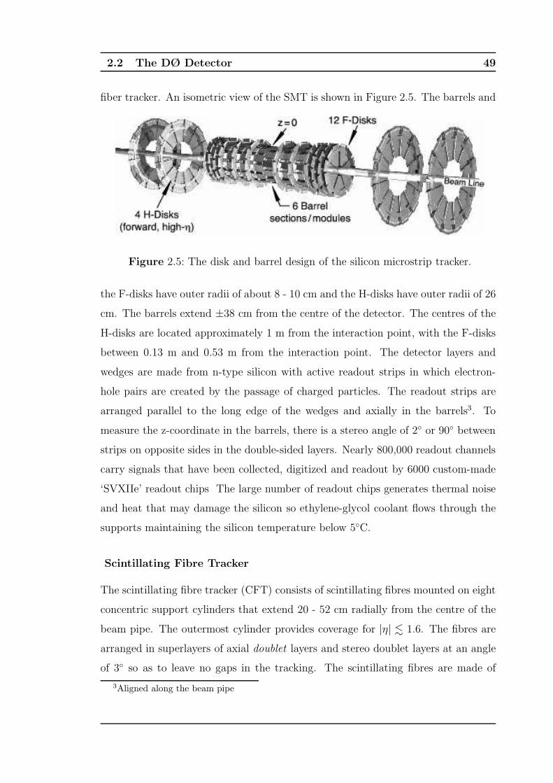
2.2 The DØ Detector 49
fiber tracker. An isometric view of the SMT is shown in Figure 2.5. The barrels and
Figure 2.5: The disk and barrel design of the silicon microstrip tracker.
the F-disks have outer radii of about 8 - 10 cm and the H-disks have outer radii of 26
cm. The barrels extend ±38 cm from the centre of the detector. The centres of the
H-disks are located approximately 1 m from the interaction point, with the F-disks
between 0.13 m and 0.53 m from the interaction point. The detector layers and
wedges are made from n-type silicon with active readout strips in which electron-
hole pairs are created by the passage of charged particles. The readout strips are
arranged parallel to the long edge of the wedges and axially in the barrels3. To
measure the z-coordinate in the barrels, there is a stereo angle of 2◦ or 90◦ between
strips on opposite sides in the double-sided layers. Nearly 800,000 readout channels
carry signals that have been collected, digitized and readout by 6000 custom-made
‘SVXIIe’ readout chips The large number of readout chips generates thermal noise
and heat that may damage the silicon so ethylene-glycol coolant flows through the
supports maintaining the silicon temperature below 5◦C.
Scintillating Fibre Tracker
The scintillating fibre tracker (CFT) consists of scintillating fibres mounted on eight
concentric support cylinders that extend 20 - 52 cm radially from the centre of the
beam pipe. The outermost cylinder provides coverage for |η| . 1.6. The fibres are
arranged in superlayers of axial doublet layers and stereo doublet layers at an angle
of 3◦ so as to leave no gaps in the tracking. The scintillating fibres are made of
3Aligned along the beam pipe
2.2 The DØ Detector 50
polystyrene, doped with an organic fluorescent dye that emits photons at 530nm
when its atoms are excited by incoming charged particles. The photons are trapped
within the polystyrene by outer layers of polymethylacrylate and fluoro-acrylic and
transmitted via clear fibre waveguides to visible light photon counters (VLPCs) [38]
to be read out. The VLPCs are avalanche photodetectors that operate at 9K and are
capable of detecting single photons and converting them into thousands of electrons,
eventually to be readout by ’SVXIIe’ chips. Light is observed only from one end of
each fibre, so, at the non-readout end there is a mirrored coating (aluminium) with
90% reflectivity.
Performance and Status
The overall momentum resolution of the tracking system is dependent on the mo-
mentum itself :
σT
pT=
√
0.0152 +0.0014pT
GeV/c
2
(2.1)
The two tracking detectors are together capable of locating the primary interaction
vertex with a resolution of 35µm along the beam line. They can tag b-quark jets4
with an impact parameter resolution better than 15µm in r − φ for particles with
transverse momentum greater than 10GeV at |η| = 0. As of May 2005, 90% of
the sensors in the SMT were functional with problems mostly occurring along the
readout chain rather than on the silicon itself.
As part of the Run IIb upgrade [33] an additional layer, Layer 0, was added to the
silicon tracker system. This additional layer is situated at small R (∼1.6cm). This is
designed to recover tracking performance and B-identification efficiency losses from
radiation damage to the silicon and aging. It will also improve impact parameter
resolution. New readout electronics for the central fibre tracker were also added to
improve tracking efficiency at high luminosity.
2.2.3 Calorimeter and pre-shower
The DØ calorimeter is designed to measure the energy of electrons, photons and
jets, to aid the identification of electrons, photons, jets and muons, and to measure
4See Section 2.2.8 for further explanation
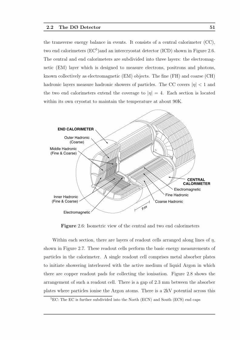
2.2 The DØ Detector 51
the transverse energy balance in events. It consists of a central calorimeter (CC),
two end calorimeters (EC5)and an intercryostat detector (ICD) shown in Figure 2.6.
The central and end calorimeters are subdivided into three layers: the electromag-
netic (EM) layer which is designed to measure electrons, positrons and photons,
known collectively as electromagnetic (EM) objects. The fine (FH) and coarse (CH)
hadronic layers measure hadronic showers of particles. The CC covers |η| < 1 and
the two end calorimeters extend the coverage to |η| = 4. Each section is located
within its own cryostat to maintain the temperature at about 90K.
Figure 2.6: Isometric view of the central and two end calorimeters
Within each section, there are layers of readout cells arranged along lines of η,
shown in Figure 2.7. These readout cells perform the basic energy measurements of
particles in the calorimeter. A single readout cell comprises metal absorber plates
to initiate showering interleaved with the active medium of liquid Argon in which
there are copper readout pads for collecting the ionisation. Figure 2.8 shows the
arrangement of such a readout cell. There is a gap of 2.3 mm between the absorber
plates where particles ionise the Argon atoms. There is a 2kV potential across this
5EC: The EC is further subdivided into the North (ECN) and South (ECS) end caps
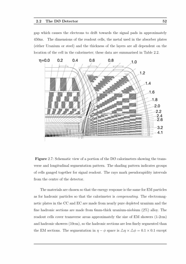
2.2 The DØ Detector 52
gap which causes the electrons to drift towards the signal pads in approximately
450ns. The dimensions of the readout cells, the metal used in the absorber plates
(either Uranium or steel) and the thickness of the layers are all dependent on the
location of the cell in the calorimeter; these data are summarised in Table 2.2.
Figure 2.7: Schematic view of a portion of the DØ calorimeters showing the trans-
verse and longitudinal segmentation pattern. The shading pattern indicates groups
of cells ganged together for signal readout. The rays mark pseudorapidity intervals
from the centre of the detector.
The materials are chosen so that the energy response is the same for EM particles
as for hadronic particles so that the calorimeter is compensating. The electromag-
netic plates in the CC and EC are made from nearly pure depleted uranium and the
fine hadronic sections are made from 6mm-thick uranium-niobium (2%) alloy. The
readout cells cover transverse areas approximately the size of EM showers (1-2cm)
and hadronic showers (10cm), so the hadronic sections are less finely segmented than
the EM sections. The segmentation in η − φ space is △η ×△φ = 0.1 × 0.1 except
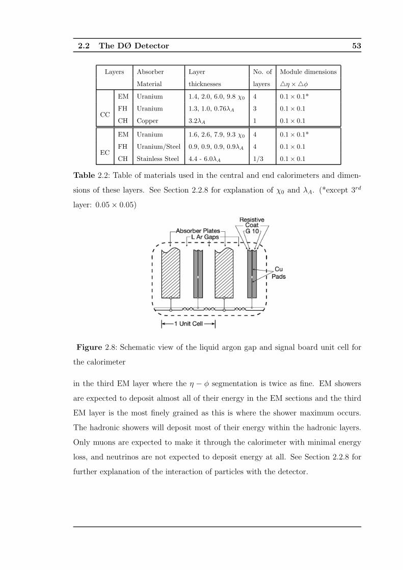
2.2 The DØ Detector 53
Layers Absorber Layer No. of Module dimensions
Material thicknesses layers △η ×△φ
CC
EM Uranium 1.4, 2.0, 6.0, 9.8 χ0 4 0.1 × 0.1*
FH Uranium 1.3, 1.0, 0.76λA 3 0.1 × 0.1
CH Copper 3.2λA 1 0.1 × 0.1
EC
EM Uranium 1.6, 2.6, 7.9, 9.3 χ0 4 0.1 × 0.1*
FH Uranium/Steel 0.9, 0.9, 0.9, 0.9λA 4 0.1 × 0.1
CH Stainless Steel 4.4 - 6.0λA 1/3 0.1 × 0.1
Table 2.2: Table of materials used in the central and end calorimeters and dimen-
sions of these layers. See Section 2.2.8 for explanation of χ0 and λA. (*except 3rd
layer: 0.05 × 0.05)
Figure 2.8: Schematic view of the liquid argon gap and signal board unit cell for
the calorimeter
in the third EM layer where the η − φ segmentation is twice as fine. EM showers
are expected to deposit almost all of their energy in the EM sections and the third
EM layer is the most finely grained as this is where the shower maximum occurs.
The hadronic showers will deposit most of their energy within the hadronic layers.
Only muons are expected to make it through the calorimeter with minimal energy
loss, and neutrinos are not expected to deposit energy at all. See Section 2.2.8 for
further explanation of the interaction of particles with the detector.
2.2 The DØ Detector 54
Intercryostat Detector and Massless Gaps Since the calorimeter is divided
into three separate sections each contained within its own cryostat, there is incom-
plete coverage in the pseudo-rapidity region 0.8 < |η| < 1.4 between the systems.
To address this problem, there are additional layers of sampling. Within the cen-
tral and end cryostats, there are single-cell readout structures called massless gaps.
In the region 1.1 < |η| < 1.4 there is a scintillator sampling detector called the
intercryostat detector (ICD) which is attached to the exterior surface of the end
cryostats and this can be seen in Figure 2.3. The ICD is a series of scintillating
tiles approximately 1.3cm thick and enclosed in light-tight aluminium boxes. Each
tile covers an area △η × △φ ≈ 0.3 × 0.4 and is further subdivided to match the
sampling geometry of the rest of the calorimeter. Although sampling can now take
place in the gaps between the calorimeter so that the overall energy resolution is
improved, the resolution in the ICD and massless gaps is poorer than that of the
main calorimeter sections.
Performance and Status
The calorimeter modules were calibrated using beams of electrons, pions and muons
between 10GeV and 150GeV before being installed in the DØ detector [39]. The
calorimeter resolution is energy dependent and of the quadratic form:
(σ
E)2
= C2 +S2
p+N2
p2(2.2)
where p is the beam momentum in GeV/c, C is a constant contribution from sys-
tematic errors such as variation in gain between readout modules, S is due to the
statistical error in sampling, and N represents energy independent contributions to
σ such as electronic and uranium noise. The calorimeter has an EM sampling reso-
lution of S = 0.157/√E, constant term of C = 0.003 and N = 0.29. The hadronic
sampling resolution is S = 0.45/√E and the constant term, C, is 0.04. The response
of the calorimeter is linear to 0.5%, and the EM/hadronic response ratio is between
1.02 and 1.09 over this range of momenta.
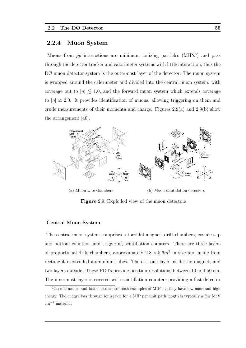
2.2 The DØ Detector 55
2.2.4 Muon System
Muons from pp interactions are minimum ionizing particles (MIPs6) and pass
through the detector tracker and calorimeter systems with little interaction, thus the
DØ muon detector system is the outermost layer of the detector. The muon system
is wrapped around the calorimeter and divided into the central muon system, with
coverage out to |η| . 1.0, and the forward muon system which extends coverage
to |η| ⋍ 2.0. It provides identification of muons, allowing triggering on them and
crude measurements of their momenta and charge. Figures 2.9(a) and 2.9(b) show
the arrangement [40].
(a) Muon wire chambers (b) Muon scintillation detectors
Figure 2.9: Exploded view of the muon detectors
Central Muon System
The central muon system comprises a toroidal magnet, drift chambers, cosmic cap
and bottom counters, and triggering scintillation counters. There are three layers
of proportional drift chambers, approximately 2.8 × 5.6m2 in size and made from
rectangular extruded aluminium tubes. There is one layer inside the magnet, and
two layers outside. These PDTs provide position resolutions between 10 and 50 cm.
The innermost layer is covered with scintillation counters providing a fast detector
6Cosmic muons and fast electrons are both examples of MIPs as they have low mass and high
energy. The energy loss through ionization for a MIP per unit path length is typically a few MeV
cm−1 material.
2.2 The DØ Detector 56
for triggering on and identifying muons, to compensate for the 750ns drift time of
the PDTs. Cosmic cap and bottom counters (scintillators) are installed on the top,
sides and bottom of the outer layer of the central muon PDTs. They provide a fast
timing signal to associate a muon in a PDT with the appropriate bunch crossing
and discriminate against the cosmic ray background.
Toroidal Magnets The stand-alone muon-system momentum measurement al-
lows for a low pT cut-off in the Level 1 muon trigger, cleaner matching with central
detector tracks and rejection of π/K decays and improves momentum resolution
for high momentum muons. The central toroid is a square annulus, 109 cm thick
whose innermost surface is 318 cm from the beam line, and is constructed in three
parts. There is a centre-bottom section, which provides a base for the calorime-
ters and central tracking detectors. There are also two c-shaped sections located
at 4546 |z| 6 610 cm. The toroid coils carry a current of 1500A resulting in an
internal field of about 1.8T.
Central Muon Drift Chambers These are made from rectangular extruded
aluminium tubes filled with a mixture of argon, methane and CF4 to reduce drift
time. These are arranged in three layers (A, B and C), with A closest to the
interaction region. Each layer has three decks of cells, with the exception of the
A-layer, which has four decks, with 24 cells, each 10.1cm across, per deck. There
is an anode wire at the centre of each cell to collect the ionisation, and these are
ganged together in pairs within a deck and readout by electronics located at one
end of each chamber. Cathode pads are located above and below the wires to
provide information on the hit position along the wire. The multi-layer nature of
the chambers allows each layer to reconstruct track segments. There are no drift
tubes at the bottom of the muon system in the A-layer as this is where the support
structure for the calorimeter lies. For each PDT hit, the following information is
recorded: the electron drift time, the difference, △T , in the arrival time of the
signal pulse at the end of the hit cell’s wire and at the end of the readout partner’s
wire, and the charge deposition on the inner and outer pads. Both △T and the
2.2 The DØ Detector 57
charge deposition are used to determine the hit position along the wire. The △Tmeasurement error depends on whether the muon passes through the cell close to
or far from the electronics - the closer to the electronics, the better the resolution.
Scintillation Counters These provide a fast detector for triggering on and iden-
tifying muons and for rejecting out-of-time backscatter from the forward direction.
In-time scintillation counter hits are matched with tracks in the CFT and the Level 1
trigger for high-pT single muon and low-pT di-muon triggers. The counters also pro-
vide the time stamp for low-pT muons that do not penetrate the toroid and so do
not reach the cosmic cap or bottom counters.
Forward Muon System
This forward muon system consists of four major parts: the end toroidal magnets,
three layers of MDTs for muon track reconstruction, three layers of scintillation
counters for triggering on events with muons and shielding around the beam pipe.
This part of the muon system receives more radiation and so MDTs were chosen
for their short electron drift time (< 132 ns), good coordinate resolution (< 1mm),
radiation hardness, high segmentation and low occupancy. Similarly to the central
muon system, the MDTs are arranged in three layers (A, B and C), with A closest
to the interaction region inside the magnet. The tubes are also arranged in three
planes in layers B and C, and in four layers in A, with the tubes mounted along
the magnetic field lines. The maximum tube length is 5830 mm in layer C. The
MDT system uses a CF4-CH4 (90%-10%) gas mixture, and the MDTs themselves
are made from extruded aluminium with stainless steel covers.
Trigger Scintillation Counters The muon trigger scintillation counters are
mounted inside and outside of the toroidal magnet. Each layer is divided into octants
containing about 96 counters. The design was optimised to provide good time
resolution and amplitude uniformity for background rejection, high muon detection
efficiency, and reasonable cost for the 5000 counters.
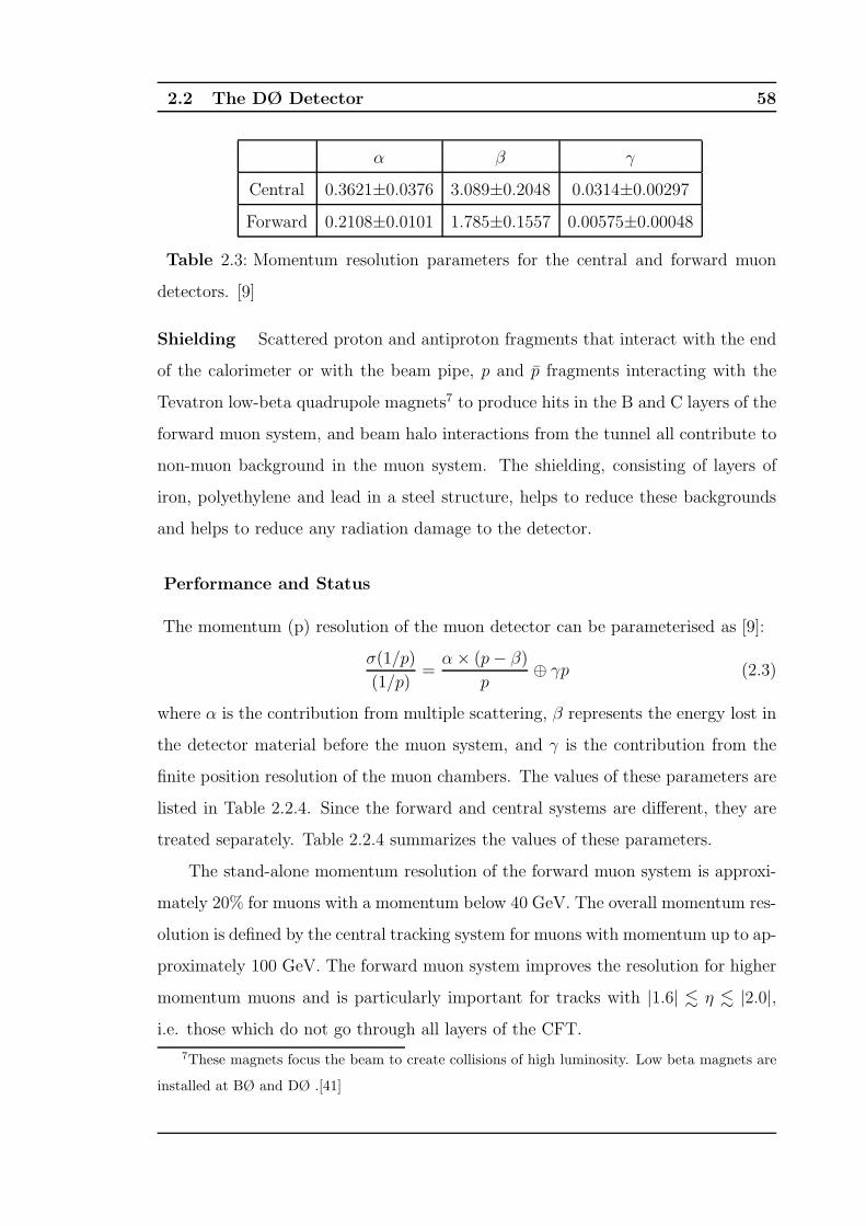
2.2 The DØ Detector 58
α β γ
Central 0.3621±0.0376 3.089±0.2048 0.0314±0.00297
Forward 0.2108±0.0101 1.785±0.1557 0.00575±0.00048
Table 2.3: Momentum resolution parameters for the central and forward muon
detectors. [9]
Shielding Scattered proton and antiproton fragments that interact with the end
of the calorimeter or with the beam pipe, p and p fragments interacting with the
Tevatron low-beta quadrupole magnets7 to produce hits in the B and C layers of the
forward muon system, and beam halo interactions from the tunnel all contribute to
non-muon background in the muon system. The shielding, consisting of layers of
iron, polyethylene and lead in a steel structure, helps to reduce these backgrounds
and helps to reduce any radiation damage to the detector.
Performance and Status
The momentum (p) resolution of the muon detector can be parameterised as [9]:
σ(1/p)
(1/p)=α× (p− β)
p⊕ γp (2.3)
where α is the contribution from multiple scattering, β represents the energy lost in
the detector material before the muon system, and γ is the contribution from the
finite position resolution of the muon chambers. The values of these parameters are
listed in Table 2.2.4. Since the forward and central systems are different, they are
treated separately. Table 2.2.4 summarizes the values of these parameters.
The stand-alone momentum resolution of the forward muon system is approxi-
mately 20% for muons with a momentum below 40 GeV. The overall momentum res-
olution is defined by the central tracking system for muons with momentum up to ap-
proximately 100 GeV. The forward muon system improves the resolution for higher
momentum muons and is particularly important for tracks with |1.6| . η . |2.0|,i.e. those which do not go through all layers of the CFT.
7These magnets focus the beam to create collisions of high luminosity. Low beta magnets are
installed at BØ and DØ .[41]
2.2 The DØ Detector 59
2.2.5 The Forward Proton Detector
This measures protons scattered at small angles (∼1 mrad) that do not interact
with the main DØ detector. A forward proton detector is necessary for access to the
full kinematics of the scattered particle. It consists of a series of momentum spec-
trometers that use the accelerator magnets in conjunction with position detectors
along the beam line. The position detectors operate a few millimetres away from
the beam and have to be moved out of the beamline during injection of protons
or antiprotons into the accelerator. The forward proton detector is not used in the
work described in this thesis.
2.2.6 Luminosity Monitor
The luminosity monitor (LM) is designed to determine the Tevatron luminosity at
the DØ interaction region. This is accomplished by detecting inelastic pp collisions
with a dedicated detector. The LM also measures beam halo rates and makes fast
measurements of the z-coordinate of the interaction vertex. The LM consists of two
arrays of 24 plastic scintillation counters with PMT readout located at z = ± 140cm,
and covers 2.7 < |η| < 4.4 . The luminosity is measured from the average number
of inelastic collisions per beam crossing detected by the LM:
L =1
σpp,eff
dN
dt(pp) (2.4)
where σpp,eff is the effective cross-section for the LM that takes into account the
acceptance and efficiency of the LM detector [42], [43]. The effective cross-section is
derived as 60.7 ± 2.4 mb [44]. Over-counting from multiple pp interactions is taken
into account by measuring the number of beam crossings with no collisions and
using Poisson statistics to determine NLM . To distinguish pp interactions from the
beam halo backgrounds, precise time-of-flight measurements are made of particles
traveling at small angles with respect to the beams to estimate the z-coordinate of
the interaction vertex. Beam halo particles traveling in the ±z direction will have
z0 ⋍ ± 140cm and are eliminated by a |z| <100 cm requirement. The luminosity
block is the fundamental unit of time for the luminosity measurement, and these
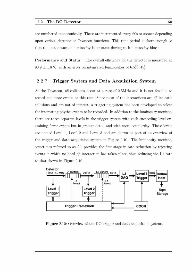
2.2 The DØ Detector 60
are numbered monotonically. These are incremented every 60s or sooner depending
upon various detector or Tevatron functions. This time period is short enough so
that the instantaneous luminosity is constant during each luminosity block.
Performance and Status The overall efficiency for the detector is measured at
90.9 ± 1.8 %, with an error on integrated luminosities of 6.5% [45].
2.2.7 Trigger System and Data Acquisition System
At the Tevatron, pp collisions occur at a rate of 2.5MHz and it is not feasible to
record and store events at this rate. Since most of the interactions are pp inelastic
collisions and are not of interest, a triggering system has been developed to select
the interesting physics events to be recorded. In addition to the luminosity monitor,
there are three separate levels in the trigger system with each succeeding level ex-
amining fewer events but in greater detail and with more complexity. These levels
are named Level 1, Level 2 and Level 3 and are shown as part of an overview of
the trigger and data acquisition system in Figure 2.10. The luminosity monitor,
sometimes referred to as L0, provides the first stage in rate reduction by rejecting
events in which no hard pp interaction has taken place, thus reducing the L1 rate
to that shown in Figure 2.10.
Figure 2.10: Overview of the DØ trigger and data acquisition systems
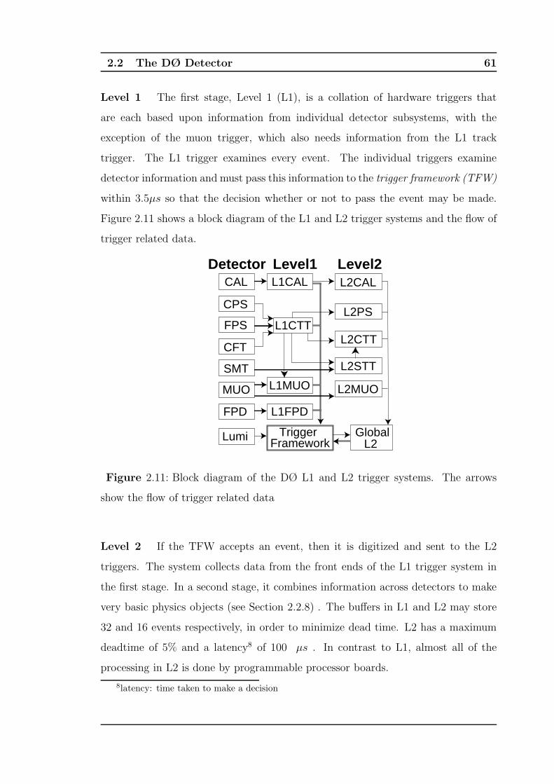
2.2 The DØ Detector 61
Level 1 The first stage, Level 1 (L1), is a collation of hardware triggers that
are each based upon information from individual detector subsystems, with the
exception of the muon trigger, which also needs information from the L1 track
trigger. The L1 trigger examines every event. The individual triggers examine
detector information and must pass this information to the trigger framework (TFW)
within 3.5µs so that the decision whether or not to pass the event may be made.
Figure 2.11 shows a block diagram of the L1 and L2 trigger systems and the flow of
trigger related data.
Level2Detector Level1
FrameworkTriggerLumi
L2Global
L2MUO
L2STT
L2CTT
L2PSL1CTT
L1MUO
L1FPDFPD
MUO
SMT
CFT
CAL L1CAL
CPS
FPS
L2CAL
Figure 2.11: Block diagram of the DØ L1 and L2 trigger systems. The arrows
show the flow of trigger related data
Level 2 If the TFW accepts an event, then it is digitized and sent to the L2
triggers. The system collects data from the front ends of the L1 trigger system in
the first stage. In a second stage, it combines information across detectors to make
very basic physics objects (see Section 2.2.8) . The buffers in L1 and L2 may store
32 and 16 events respectively, in order to minimize dead time. L2 has a maximum
deadtime of 5% and a latency8 of 100 µs . In contrast to L1, almost all of the
processing in L2 is done by programmable processor boards.
8latency: time taken to make a decision
2.2 The DØ Detector 62
Level 3 The Level 3 trigger provides additional rejection of events to enrich the
physics samples and to reduce the rate of events to be stored on tape to 50Hz for
offline analysis. The accept rate is limited by the capabilities of and cost of data
storage and offline computing. L3 is entirely software-based, reads out information
from the entire detector and is run on a dedicated PC farm. Software tools build
on the basic physics objects of L2 and decisions are using these objects and the
relationships between them such as invariant mass. The filtering software can be
changed as physics objectives or the operating parameters of the experiment change.
The list of filters and their criteria is known as a trigger list and is assigned a version
number.
2.2.8 Object Identification
This section briefly describes how different particles interact with the DØ detector.
It also explains how they are measured, calibrated, and the terminology associated
with them. It also describes certain detector objects that describe particle properties
and are useful in analyses.
Electrons and photons
Electrons and positrons lose energy primarily through ionisation and bremsstrahlung
[8]. Bremsstrahlung is the radiation emitted by a charged particle when accelerated
transversely when passing through the field of atomic nuclei. This results in a shower
of electron-positron pairs and photons. The photons themselves produce electron-
positron pairs which further shower in the fields of the nuclei. For electrons above
the critical energy of E ≈ 610MeV/(1.2 +Z) (where Z is the atomic number of the
material), bremsstrahlung is the dominant process. Similarly, a shower is produced
if the primary particle is a photon. A radiation length, χ0, can be defined, over
which the electron’s energy will be reduced by a factor of 1/e [8]:
χ0 =716gcm−2A
Z(Z + 1) ln(287/√Z)
(2.5)
2.2 The DØ Detector 63
The reconstruction of electrons and other EM objects starts in the calorimeter
with clusters of energy deposits in cells in the EM layers (EEM), and the first
hadronic layer (Ehad). A cluster is defined to be a group of 3×3 towers with energy
greater than 500MeV [46]. The primary method to reconstruct electrons proceeds
with a simple cone algorithm, with R=0.2, which is then applied to the seed-towers
with ET > 1.5GeV. At this point, photons and electrons may be differentiated since
electrons are expected to interact with the tracking system, and photons are not.
An electron track, which must have pT > 1.5GeV, should point in the same direction
as the electron’s EM shower, and have a momentum that matches the energy of the
shower. This is measured using a χ2 match quantity [47]:
χ2spatial = (
δφ
σφ)2 + (
δz
σz)2 + (
ET/pT − 1
σET /pT
)2 (2.6)
Electrons require a χ2 probability of greater than 10−2. The track now associated
with the electron provides the θ and φ coordinates, and its total energy is taken from
the calorimeter measurements; combining them gives the momentum. Without a
track match, these coordinates are reconstructed from the primary vertex and the
object’s position within the third EM layer. Several additional variables are useful
in characterising electrons and photons with high efficiency :
• Isolation (fIso) Electrons and photons (and the showers they produce) are
usually isolated from other particles in the calorimeter, unlike hadrons which
are usually in jets of particles. The measure of this isolation, the isolation
fraction, dependent on the total energy within the cone from all layers used,
Etot, is given by:
fiso =Etot(R < 0.4) − EEM(R < 0.2)
Etot(R < 0.2)(2.7)
where R defines the size of the cone.
• EM fraction, fEM This uses the measurement of the energy deposited in the
first hadronic layer, with the energy deposited in the EM layers to calculate
the fraction of energy deposited in the EM calorimeter: EMF = EEM/Etot.

2.2 The DØ Detector 64
• Coarse Hadronic Fraction, fCH In a similar way to fEM , the coarse
hadronic fraction is the fraction of energy deposited in the coarse hadronic
layers.
• Hot Fraction This is the ratio of the transverse energies of the calorimeter
tower with the highest energy, to the tower with the second highest energy.
This cut, along with the following two variables, n90 and f90, are used to elim-
inate hot cells in the calorimeter that have been misidentified as EM objects.
• n90 This is the total number of towers that make up 90% of the EM shower
energy.
• f90 Similar to n90, this is the fraction of the number of cells comprising 90%
of the EM object energy.
• HMatrix (HMx8 ) This measures how similar the shower is to an electron
shower. There are eight correlated observables used in this shower shape anal-
ysis that include EM energy fractions, the total EM energy, vertex z-position
and transverse shower width in φ and z. The 8×8 covariance matrix is a mea-
sure of the shower similarity. The HMatrix is the inverse of this covariance
matrix. It is calculated for each tower in η [48].
The offline electron reconstruction efficiencies in data, calculated from Z → e+e−
events in the CC is 84.1% ± 0.9%, and in the EC, 91.5% ± 1.3% [49]. Other types of
reconstructed electrons that are less commonly used are the road and SEM electrons,
and these are described in Section 4.3.
There are several sources of background which may be mistakenly identified as
electrons [50]
• π0 showers which overlap with a track from a charged particle.
• Photons which convert to e+e−pairs.
• π± which undergo charge exchange in the detector material.
• Fluctuations of hadronic shower shapes.
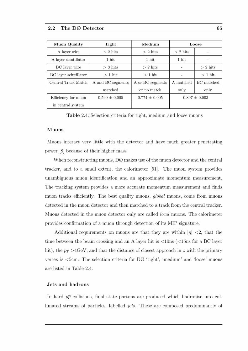
2.2 The DØ Detector 65
Muon Quality Tight Medium Loose
A layer wire > 2 hits > 2 hits > 2 hits -
A layer scintillator 1 hit 1 hit 1 hit -
BC layer wire > 3 hits > 2 hits - > 2 hits
BC layer scintillator > 1 hit > 1 hit - > 1 hit
Central Track Match A and BC segments A or BC segments A matched BC matched
matched or no match only only
Efficiency for muon 0.599 ± 0.005 0.774 ± 0.005 0.897 ± 0.003
in central system
Table 2.4: Selection criteria for tight, medium and loose muons
Muons
Muons interact very little with the detector and have much greater penetrating
power [8] because of their higher mass
When reconstructing muons, DØ makes use of the muon detector and the central
tracker, and to a small extent, the calorimeter [51]. The muon system provides
unambiguous muon identification and an approximate momentum measurement.
The tracking system provides a more accurate momentum measurement and finds
muon tracks efficiently. The best quality muons, global muons, come from muons
detected in the muon detector and then matched to a track from the central tracker.
Muons detected in the muon detector only are called local muons. The calorimeter
provides confirmation of a muon through detection of its MIP signature.
Additional requirements on muons are that they are within |η| <2, that the
time between the beam crossing and an A layer hit is <10ns (<15ns for a BC layer
hit), the pT >4GeV, and that the distance of closest approach in z with the primary
vertex is <5cm. The selection criteria for DØ ‘tight’, ‘medium’ and ‘loose’ muons
are listed in Table 2.4.
Jets and hadrons
In hard pp collisions, final state partons are produced which hadronise into col-
limated streams of particles, labelled jets. These are composed predominantly of
2.2 The DØ Detector 66
photons, pions and kaons and they are detected when the particles deposit energy
in the calorimeter cells. Jets are then reconstructed from these energy deposits using
the D0Run II jet cone algorithm [52], [53]. To relate the measured jet energy back
to the energy of the final state partons, a jet energy scale is derived to correct for
the distortions to the measured energy by various detector and physics effects.
Hadrons interact with the nuclei of the detector. A length scale, the interaction
length[8], similar to the radiation length of electrons, is given approximately by:
λI ≈ 35A13gcm−2 (2.8)
Hadrons produce showers of hadronic particles, mostly pions and nucleons, which in
turn interact with the nuclei of the detector producing a cascade. These showers are
measured as jets within the calorimeter; clustering algorithms group the cells with
energy deposits from the EM and hadronic layers. Most jets at DØ are reconstructed
using the Run II Cone algorithm [54] Cones have their origins at an interaction point
and extend outwards containing the jet particles. They have a fixed △R in η − φ
space. The cone jet corresponds to a “stable” orientation of the cone around energy
clusters in the calorimeter. A seed-based algorithm is applied which uses seeds
and midpoints of seeds as starting points for finding these stable cones. The seeds
are preclusters of calorimeter towers, instead of single (out of 5000) towers, which
reduce the time taken to find all stable cones. The Run II cone algorithm is divided
into three stages: clustering, addition of midpoints, and merging-splitting. The
clustering stage is based on the Simple Cone Algorithm and it forms the preclusters
of towers which are used to form protojets. Following this, protojets are also searched
for around the midpoints of any two already existing protojets if they are more than
△Rcone (usually R=0.5) apart. Lastly, as protojets often share items (clusters) of
energy, cones are merged or split according to how the clusters are shared. This
is to avoid double counting of energy. If a protojet shares one or more items with
another protojet and these represent 50% or more of the energy of the other jet,
then the shared clusters are assigned to that other jet, and the first jet is removed.
If the fraction of shared energy is smaller than 50% of either jet, then the two jets
are split and the items are assigned to the nearest jets.
2.2 The DØ Detector 67
The jet algorithm is not perfect, for example some of the energy of the jet may
lie outside the cone, the cone may contain energy from calorimeter noise etc. So
a correction is made for these effects and an overall calorimeter response to jets is
derived. Together, along with a number of other, smaller corrections, make up the
jet energy scale which is discussed in detail in Chapter 3. The jet energy resolution
is similar in form to the calorimeter resolution and is measured from (γ + jets) and
dijet data [55]:
(σET
ET
)2
=N
ET
⊕ S√ET
⊕ C (2.9)
where C is a correction for the jet energy scale, S is a correction for jet energy that
ends up outside the jet cone, and N is due to instrumental noise and other detector
effects. The efficiency of both identifying and reconstructing a jet depends on the
calorimeter region and is as high as 99% in the central region, and as low as 95% in
the ICR, and is 98% in the end caps.
Detector Objects
E/T , pT and neutrinos Since energy must be conserved in the collisions inside
the detector, any missing energy is a sign of neutrinos or other non-interacting
particles. We often use only the components of energy and momenta perpendicular
to the z-axis because it is difficult to measure accurately the components of these
quantities when the particles escape down the beam-pipe in the z-direction. So it
is the missing transverse energy that we use to measure non-interacting particles.
The missing transverse energy, E/T , is the negative magnitude of the vector sum of
the calorimeter tower transverse energies and is defined as:
E/T = −(∑
i
(Exi),∑
i
(Eyi)) (2.10)
where Exi and Eyi are defined the x and y components of the tower energies within
|η| < 4.5. Before the E/T can be used in an analysis, it must be adjusted to account
for the corrections that are applied to the other physics objects in the event [56]:
noisy cells in the coarse hadron calorimeter, the EM scale, the jet energy scale, and
for muons detected only in the muon system. Where jets are concerned, the scalar
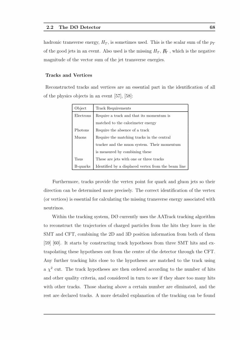
2.2 The DØ Detector 68
hadronic transverse energy, HT , is sometimes used. This is the scalar sum of the pT
of the good jets in an event. Also used is the missing HT , H/T , which is the negative
magnitude of the vector sum of the jet transverse energies.
Tracks and Vertices
Reconstructed tracks and vertices are an essential part in the identification of all
of the physics objects in an event [57], [58]:
Object Track Requirements
Electrons Require a track and that its momentum is
matched to the calorimeter energy
Photons Require the absence of a track
Muons Require the matching tracks in the central
tracker and the muon system. Their momentum
is measured by combining these
Taus These are jets with one or three tracks
B-quarks Identified by a displaced vertex from the beam line
Furthermore, tracks provide the vertex point for quark and gluon jets so their
direction can be determined more precisely. The correct identification of the vertex
(or vertices) is essential for calculating the missing transverse energy associated with
neutrinos.
Within the tracking system, DØ currently uses the AATrack tracking algorithm
to reconstruct the trajectories of charged particles from the hits they leave in the
SMT and CFT, combining the 2D and 3D position information from both of them
[59] [60]. It starts by constructing track hypotheses from three SMT hits and ex-
trapolating these hypotheses out from the centre of the detector through the CFT.
Any further tracking hits close to the hypotheses are matched to the track using
a χ2 cut. The track hypotheses are then ordered according to the number of hits
and other quality criteria, and considered in turn to see if they share too many hits
with other tracks. Those sharing above a certain number are eliminated, and the
rest are declared tracks. A more detailed explanation of the tracking can be found
2.2 The DØ Detector 69
in reference [61]. Once tracks have been found, they are extrapolated through the
detector and linked to physics objects using the Global Tracking algorithm, [60].
The tracking efficiency depends on the location of the track within the tracking
system and the pT of the particle. For a track with pT above 10GeV, the efficiency
is between 96% and 99%, with a fake rate of around 2%. For tracks below 10GeV,
the efficiency is approximately 92% with a fake rate of about 1% [62].
At DØ vertex detection depends on track identification, and there are two types
of vertices that are constructed in each event: a primary vertex, and secondary
vertices. The primary vertex is the main interaction point of the collision and must
lie along the beam line within |z| < 60cm. It is reconstructed from good quality
tracks only with an average efficiency of 98%, measured on multijet data. The
primary vertex may be located to within 15µm in x,y and to within 30µm in z.
The B-meson has a relatively long lifetime so it may travel far enough before
decaying that its decay vertex may be resolved by the tracking system. This decay
vertex is called the secondary vertex and is found using the secondary vertex tagger
(SVT) algorithm [63], [64]. The identification of jets originating from b-quarks
is called b-tagging and there are several other algorithms for identifying b-jets by
assigning a probability to the jet that came from a b-quark. This process is described
in more detail in Chapter 5.
DØ Software and Terminology
DØ analysis and processing software versions are referred to by their release number
in the format pXX, or pXX.XX.XX, for example p14, p16.07.00 [65]. A change in
release version marks major changes to the software, or introduction of new algo-
rithms or a new set of reprocessing. Any specific corrections for problems discovered,
such as bugs in the software, or corrections for hardware problems may be named
in the same fashion, or be referred to by the package name, such as d0correct [66].
Most of the analysis at DØ is carried out on data stored in the thumbnail format
[67] which requires about 10kb per event.
The trigger system uses a single version of the trigger list at any one time.
2.2 The DØ Detector 70
These trigger lists are updated to take into account changing physics programmes,
increasing luminosity and the aging of the detector. These are labelled v12, v13 etc
[68].
2.2.9 Overall Current Detector Performance and Status
The DØ Run II daily data taking efficiency is shown in Figure 2.12(a), and Fig-
ure 2.12(b) shows the luminosity delivered to and recorded by DØ to date. Since
the start of Run II, DØ has recorded 1.3fb−1 data, and has operated at a daily
efficiency around 85% for most of Run II. The increased luminosities of Run IIb
required upgrades to the silicon tracker and the trigger system and in 2002 upgrade
programmes were approved. The upgrades were installed at the end of 2005 and
the Run IIb detector upgrades are described in detail in [33]. The trigger system
upgrades included a replacement L1 Calorimeter module, a new module that uses
both tracking and calorimeter information, more L2 modules and processors, and
additional L3 processors and online storage. An additional layer, Layer 0, was also
added to the silicon tracker at about 1.6cm from the beam line, as mentioned earlier
in the chapter.
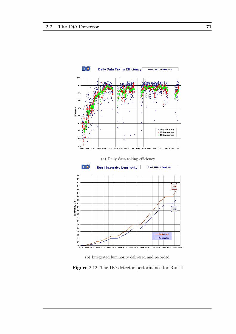
2.2 The DØ Detector 71
(a) Daily data taking efficiency
(b) Integrated luminosity delivered and recorded
Figure 2.12: The DØ detector performance for Run II

3 The Jet Energy Scale 72
Chapter 3
The Jet Energy Scale
3.1 Introduction
Almost all physics programmes at DØ involve jets so it is important that their
characteristics are well understood and that their energies and other properties are
accurately measured. For example, the Tevatron is the only collider where top
quarks are produced directly and currently the errors from the jet energy scale
dominate the error in the top mass measurement [69]. The Jet Energy Scale (JES)
is a calibration that allows the energies of reconstructed collider jets to be related
back to those of the final state particle jets1, on average.
In Run I, the jet energy scale was based on transverse energy conservation in
(γ + jets) events. Now, in Run II, with the larger datasets, the jet energy scale can
be derived using Z(e+e−)+jets events. In this chapter, the calorimeter response to
jets is derived using p14 MC and Pass 22 data events and compared to the official
response from (γ + jets) events. This formed part of the verification of version 4.2
[70] of the official DØ JES. Before the (Z + jets) response was calculated, some
1The particle level jet energy is defined as the jet energy found from final state partons using
a cone algorithm as described in Chapter 2. Particle jets cannot be seen in data, but they can be
defined in Monte Carlo samples.2Pass 2 denotes the version of data reprocessing and the corrections applied. See http:
//www-d0.fnal.gov/Run2Physics/cs/skimming/pass2.html.

3.2 The Jet Energy Scale 73
other, independent corrections were made to the jets using v4.2 of the jet energy
scale (see Section 3.3.2 for more detail). Closure tests are also performed on the
(γ + jets) JES versions 4.2 (and 5.1) using (Z + jets) events. The closure tests
using JES v4.2 are shown in this chapter. This work was carried out in 2003 and
2004 when DØ had collected only about 140pb−1 of data.
3.2 The Jet Energy Scale
Before measurement, the jet energy is affected primarily by the calorimeter re-
sponse to different particles. Although EM and hadronic particles interact with the
calorimeter though different physics processes, the calorimeter response is nearly
compensating. The jet energy is also distorted by energy losses in uninstrumented
regions, uranium decays leaving energy deposits in the argon, spectator interactions,
and reconstruction effects from the cone algorithm. The response for (γ + jets)
events is obtained by using the Missing ET Projection Fraction Method (MPFM)
which was first used in Run I and is described in [71]. Since the topology of (Z + jets)
events is similar to that of (γ + jets) events, the same procedure can be used. The
JES is implemented in a software package, jetcorr [72], which calculates the jet cor-
rections ‘on the fly’ during an analysis and also provides statistical and systematic
errors for the jet energies.
The factors affecting jet energies are summarized in Equation 3.1. This shows
the relationship of the measured energy of the jet in the calorimeter (Emeasjet ) to the
particle jet energy (Eptljet) as a function of several variables including luminosity, L,
and jet η:
Eptljet =
Emeasjet − Eo(R, η,L)
Rjet(R, η,L)Rcone(R, η,L)(3.1)
Where:
• Eo is the offset energy. This is any energy measured as part of the jet not due
to the hard interaction itself.
• Rjet is the calorimeter response to the hadronic jet known as the jet energy
3.2 The Jet Energy Scale 74
response and this is derived in the next section.
• Rcone is the fraction of the particle jet energy that is contained within the jet
reconstruction cone. This is corrected for by the showering correction.
Offset Correction The offset correction, Eo(R, η,L), includes any energy that
does not come directly from the hard interaction itself, such as uranium noise,
remains of previous bunch crossings (pile-up energy), additional interactions, and
the underlying physics event3. This is dependent on the luminosity, L , and increases
with the jet cone size, R. Eo is also dependent on the physics η. The total offset
energy correction can be considered as the sum:
Eo = (1 + 〈EZB〉)Eue + Enoise + Epile
= Eue + 〈NZB〉Eue + Enoise + Epile (3.2)
where 〈NZB〉 is the average number of hard core interactions in a zero-bias event, Eue
is the energy from the underlying physics event, 〈NZB〉Eue is the energy associated
with additional pp interactions, Enoise represents the noise from uranium decay, and
Epile is the pile-up energy. 〈NZB〉 may be calculated from the probability, which
follows a Poisson distribution, of a hard core collision at a given luminosity.
Showering Correction The showering correction compensates for the fraction of
jet energy that falls outside the reconstruction cone as the particles interact with the
calorimeter. This also corrects for energy that originates from outside the cone, but
that ends up inside, perhaps bent by the magnetic field. The showering correction is
derived from both MC and data using jet energy density profiles. It is not possible
to directly determine the instrumental showering contribution because energy left
outside the cone that is part of the jet may also be associated with gluon emission or
fragmentation at the particle level (physics out-of-cone). This contribution must be
determined from Monte Carlo events using information about the particles within
3Underlying physics event: defined as the energy coming from spectators to the hard proton
interaction.
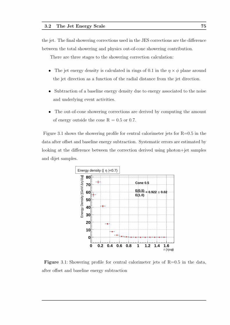
3.2 The Jet Energy Scale 75
the jet. The final showering corrections used in the JES corrections are the difference
between the total showering and physics out-of-cone showering contribution.
There are three stages to the showering correction calculation:
• The jet energy density is calculated in rings of 0.1 in the η × φ plane around
the jet direction as a function of the radial distance from the jet direction.
• Subtraction of a baseline energy density due to energy associated to the noise
and underlying event activities.
• The out-of-cone showering corrections are derived by computing the amount
of energy outside the cone R = 0.5 or 0.7.
Figure 3.1 shows the showering profile for central calorimeter jets for R=0.5 in the
data after offset and baseline energy subtraction. Systematic errors are estimated by
looking at the difference between the correction derived using photon+jet samples
and dijet samples.
)φxηr (0 0.2 0.4 0.6 0.8 1 1.2 1.4 1.6
]φ∆/η
∆E
nerg
y D
ensi
ty [G
eV/
0
10
20
30
40
50
60
70
80
|<0.7)ηEnergy density (|
Cone 0.5
0.02± = 0.922 E(1.0)E(0.5)
Figure 3.1: Showering profile for central calorimeter jets of R=0.5 in the data,
after offset and baseline energy subtraction
3.3 Jet Response 76
3.3 Jet Response
3.3.1 Missing ET Projection Fraction Method
The jet energy response (Rjet) is derived using (γ + jets) or (Z + jets) data and
Monte Carlo events where there is one photon balanced in pT by one or more jets,
relying on the much more accurately-calibrated measurement of the photon and
electron energy scales, the fact that we can measure jet direction very well, and
that in a perfect calorimeter there should be no missing energy perpendicular to
the pp collision direction. Any non-zero missing transverse energy would usually
indicate the presence of a neutrino or a muon which has not deposited its energy
in the calorimeter. Instead, as the calorimeter response is imperfect, a non-zero
E/T measures the overall imbalance of transverse energy in the calorimeter due to
different responses to photons and jets. This can be used to measure the response,
Rrecoil, relative to the precisely calibrated photon response, which is assumed to be
close to the particle level response. Here, Rrecoil is the calorimeter response to jets
and includes already the showering and offset energy corrections. If there is only a
single photon (or Z boson) and a single jet in the event, and if there were no energy
distortions from showering or offset energies, then Rrecoil is exactly EmeasT,jet /E
particleT,jet .
For events in which the photons are back-to-back4, then Rrecoil ≈ Rjet. In (γ + jets)
events, the photon (−→E Tγ)
5 and recoil transverse energies (−→E T,recoil) satisfy:
−→E T,γ +
−→E T,recoil = 0 (3.3)
However, in reality, the responses are both less than unity, and the resulting deficit
in ET is the measured E/T :
−→Emeas
T,γ +−→Emeas
T,recoil = −−→E/T
meas (3.4)
where−→Emeas
T,γ = Rem−→E T,γ and
−→Emeas
T,recoil = Rrecoil−→E T,recoil.
4back-to-back: where the azimuthal angle between the objects is π5Since the MPFM is the same for both (γ + jets) and (Z + jets) events, in this section, γ is
used interchangeably with Z
3.3 Jet Response 77
The EM scale is used to correct−→Emeas
T,γ and so Equation 3.4 becomes:
−→E T,γ +Rrecoil
−→E T,recoil = −−→
E/T (3.5)
−→E T,γ +RrecoilnT,γ
−→E T,recoil = −nT
−→E/T (3.6)
1 +RrecoilnT,γ
−→E T,recoil−→E T,γ
= − nT
−→E/T
ET,γ(3.7)
where nT,γ =−→E T,γ/|
−→E T,γ| so that Equation 3.3 can be rewritten as:
Rrecoil = 1 +
−→E/T · nT,γ
ET,γ
(3.8)
The topology of (Z + jets) events (where the Z decays to an e+e−pair) is similar
to that of (γ + jets) events, the missing ET projection fraction method may thus
be used to derive the response, substituting−→E T,Z for
−→E Tγ in Equations 3.3 to 3.8.
The Energy Estimator, E′
The response is dependent on the jet energy, not its transverse component be-
cause the EM-hadronic response ratio and the particle composition of the jets are
energy dependent. However, it is difficult to measure directly Rjet as a function of
Emeasjet as Emeas
jet is biased by many things including trigger and reconstruction effects,
event topology, and energy resolutions for photons/electrons and jets. Instead, the
response may be binned in the better-measured quantity, the energy estimator, E′:
E ′ = ETγ · cosh(η) (3.9)
where ETγ includes the electromagnetic scale correction. This helps reduce the biases
and energy smearing effects as both the ETγ and the jet η can be measured more
precisely than Emeasjet . Figures 3.2(a) and 3.2(b) show the E ′ → Emeas
jet mapping for
data and MC event samples respectively, divided into the three calorimeter regions,
CC, EC, and ICR. The mapping of actual jet energy to E′ varies between the three
regions.
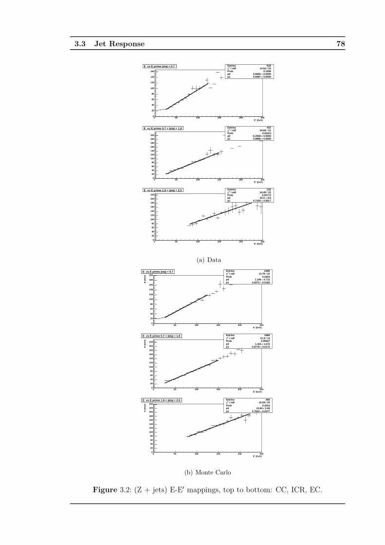
3.3 Jet Response 78
E’ (GeV)0 50 100 150 200 250
0
20
40
60
80
100
120
140
160
E vs E prime |eta| < 0.7 Entries 616 / ndf 2χ 14.52 / 10
Prob 0.1506p0 0.0000± 0.6666 p1 0.0000± 0.9487
E vs E prime |eta| < 0.7
E’ (GeV)0 50 100 150 200 250
0
20
40
60
80
100
120
140
160
180
200
220
E vs E prime 0.7 < |eta| < 1.8 Entries 415 / ndf 2χ 24.84 / 13
Prob 0.02421p0 0.0000± -0.2938 p1 0.0000± 0.8886
E vs E prime 0.7 < |eta| < 1.8
E’ (GeV)0 50 100 150 200 250
0
20
40
60
80
100
120
140
160
180
200
220
E vs E prime 1.8 < |eta| < 2.5 Entries 120 / ndf 2χ 24.46 / 15
Prob 0.05772p0 8.6± 20.5 p1 0.0617± 0.7165
E vs E prime 1.8 < |eta| < 2.5
(a) Data
E’ (GeV)0 50 100 150 200 250
E (
GeV
)
0
20
40
60
80
100
120
140
160
180
200
E vs E prime |eta| < 0.7 Entries 2486 / ndf 2χ 13.76 / 10
Prob 0.1844p0 0.713± 1.146 p1 0.0165± 0.9472
E vs E prime |eta| < 0.7
E’ (GeV)0 50 100 150 200 250
E (
GeV
)
0
20
40
60
80
100
120
140
160
180
200
220
E vs E prime 0.7 < |eta| < 1.8 Entries 1688 / ndf 2χ 21.8 / 13
Prob 0.05847p0 1.072± 1.431 p1 0.0172± 0.8778
E vs E prime 0.7 < |eta| < 1.8
E’ (GeV)0 50 100 150 200 250
E (
GeV
)
0
20
40
60
80
100
120
140
160
180
200
220
240
E vs E prime 1.8 < |eta| < 2.5 Entries 458 / ndf 2χ 15.28 / 15
Prob 0.4314p0 5.28± 15.84 p1 0.0377± 0.7932
E vs E prime 1.8 < |eta| < 2.5
(b) Monte Carlo
Figure 3.2: (Z + jets) E-E′ mappings, top to bottom: CC, ICR, EC.

3.3 Jet Response 79
Event Samples and Selection
The calorimeter response to jets in Z(e+e−) + jets events was calculated with Monte
Carlo and Pass 2 data, using software version p14 [73], and d0correct6 v8.0 [66]. For
data, 15 million Pass 2 events were used, skimmed so that each event contains two
EM objects with pT >7GeV. Closure tests were performed on the jet energy scale
given in the v6.0 JetCorr package. A good run list was used to eliminate bad events
which may contain information from noisy or malfunctioning subdetectors. For the
Monte Carlo studies, 289,000 inclusive Z+jet(s) plate7 events generated by Pythia
(v.6.155 [74]), with a kinematical cut on the Z mass of 60GeV < mZ <130GeV were
used.
The response is measured from simulated and data event samples that have
been selected using a set of criteria designed to pick ‘true’ (Z + jets) events but
remove systematic biases and unwanted backgrounds. The cuts are applied in three
stages. Firstly, general event cuts are applied to choose ‘clean’ events, secondly cuts
are applied to remove backgrounds, and lastly cuts are applied to ensure that the
event has the correct topology. For a detailed explanation of the selection criteria
used in this section, refer to Section 2.2.8. The following criteria were applied to
both data and Monte Carlo events, and the cutflow tables are given in Table 3.1.
General Cuts Since the Z boson in each event is reconstructed from two elec-
trons8 emitted back-to-back in the Z rest frame, each event must have:
• Two EM objects, both of which must be identified as an EM object with a
track match.
• The EM objects must have opposite charge signs to ensure that it is an
e+e−pair.
6This is a software package that carries out all the post processing (corrections, certifications)
for EM, muon, jet and E/T objects.7Plate MC events are those where the calorimeter has been simulated as a series of uranium
and argon plates.8In this section electron is used interchangeably with positron, unless specified otherwise
3.3 Jet Response 80
Furthermore, events must be fully within the fiducial regions of the calorimeter.
To avoid problems associated with measuring jet energies at low ET (low-ET bias),
only events with ET >25GeV are used. Lastly, primary vertices at large distances
from the detector centre can distort ET measurements so it is required that the
primary vertex must be within |z| <50cm and that it must have at least 5 tracks
associated with it.
Background cuts The official p14 recommended object-quality selection cuts9
from the EM Object [75] and Jet Identification Working Groups [76] were applied
to ensure that a good sample of electrons and jets was collected:
Electrons Jets
• fEM > 0.9 • 0.05 < fEM < 0.9
• fIso < 0.15 • fCH < 0.4
• HMx8 < 20 • Hot fraction < 10.0
• n90 > 1.0
• f90(= n90/number of towers):
f90 < (0.8 - 0.5×fCH)or fCH <0.1
The jets were reconstructed with the cone algorithm as described in Section
2.2.8, using R=0.5 cones, and with v1.2 of the recommended cuts. The electrons
were simple cone electrons, corrected using the p14 electron energy scale10. The
background is made up of instrumental backgrounds where highly EM jets are mis-
taken for electron showers, and physics backgrounds from other similar decay chan-
nels. To eliminate instrumental backgrounds, a cut is placed on the electrons to
ensure they are well-isolated from both other EM objects and highly electromag-
netic jets (mostly π0 jets). Jets with a high EM component bias the measurement
of Rjet and they may be identified and rejected using a cut on the HMatrix value
for the EM object. This cut removes many events but discriminates well between
9For definitions of physics and detector objects please refer to Chapter 2.10This EM scale correction is also included in the E/T in each event.
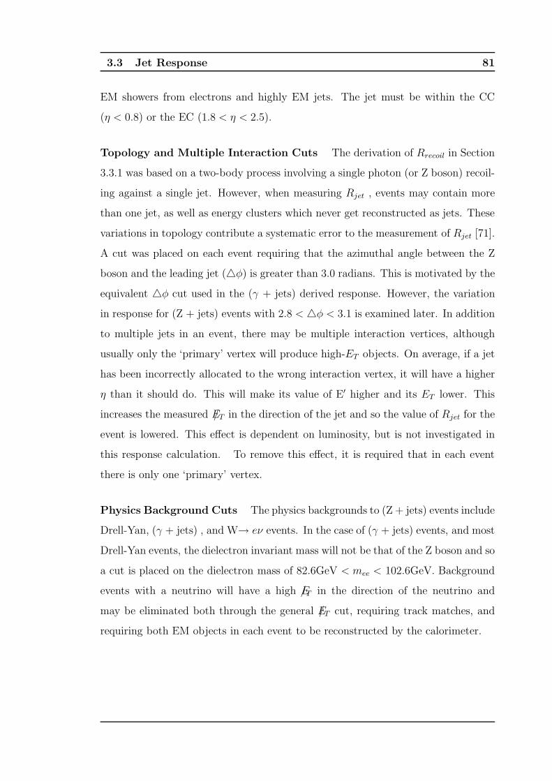
3.3 Jet Response 81
EM showers from electrons and highly EM jets. The jet must be within the CC
(η < 0.8) or the EC (1.8 < η < 2.5).
Topology and Multiple Interaction Cuts The derivation of Rrecoil in Section
3.3.1 was based on a two-body process involving a single photon (or Z boson) recoil-
ing against a single jet. However, when measuring Rjet , events may contain more
than one jet, as well as energy clusters which never get reconstructed as jets. These
variations in topology contribute a systematic error to the measurement of Rjet [71].
A cut was placed on each event requiring that the azimuthal angle between the Z
boson and the leading jet (△φ) is greater than 3.0 radians. This is motivated by the
equivalent △φ cut used in the (γ + jets) derived response. However, the variation
in response for (Z + jets) events with 2.8 < △φ < 3.1 is examined later. In addition
to multiple jets in an event, there may be multiple interaction vertices, although
usually only the ‘primary’ vertex will produce high-ET objects. On average, if a jet
has been incorrectly allocated to the wrong interaction vertex, it will have a higher
η than it should do. This will make its value of E′ higher and its ET lower. This
increases the measured E/T in the direction of the jet and so the value of Rjet for the
event is lowered. This effect is dependent on luminosity, but is not investigated in
this response calculation. To remove this effect, it is required that in each event
there is only one ‘primary’ vertex.
Physics Background Cuts The physics backgrounds to (Z + jets) events include
Drell-Yan, (γ + jets) , and W→ eν events. In the case of (γ + jets) events, and most
Drell-Yan events, the dielectron invariant mass will not be that of the Z boson and so
a cut is placed on the dielectron mass of 82.6GeV < mee < 102.6GeV. Background
events with a neutrino will have a high E/T in the direction of the neutrino and
may be eliminated both through the general E/T cut, requiring track matches, and
requiring both EM objects in each event to be reconstructed by the calorimeter.
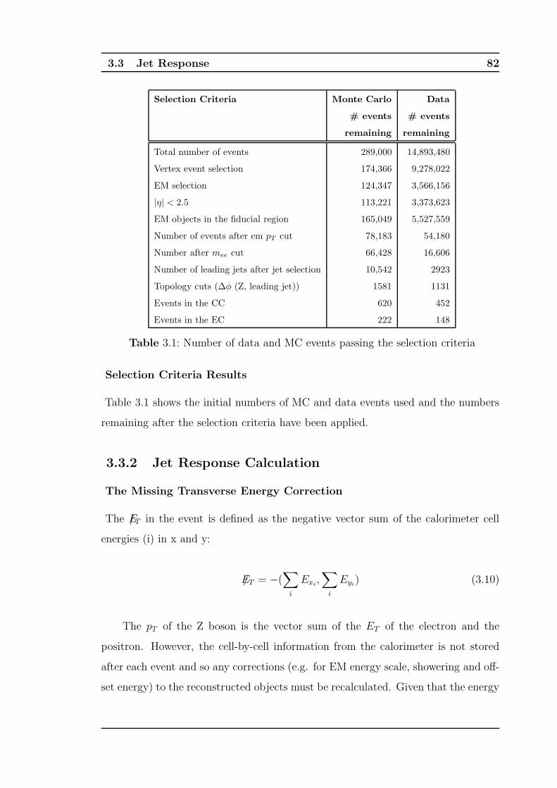
3.3 Jet Response 82
Selection Criteria Monte Carlo Data
# events # events
remaining remaining
Total number of events 289,000 14,893,480
Vertex event selection 174,366 9,278,022
EM selection 124,347 3,566,156
|η| < 2.5 113,221 3,373,623
EM objects in the fiducial region 165,049 5,527,559
Number of events after em pT cut 78,183 54,180
Number after mee cut 66,428 16,606
Number of leading jets after jet selection 10,542 2923
Topology cuts (∆φ (Z, leading jet)) 1581 1131
Events in the CC 620 452
Events in the EC 222 148
Table 3.1: Number of data and MC events passing the selection criteria
Selection Criteria Results
Table 3.1 shows the initial numbers of MC and data events used and the numbers
remaining after the selection criteria have been applied.
3.3.2 Jet Response Calculation
The Missing Transverse Energy Correction
The E/T in the event is defined as the negative vector sum of the calorimeter cell
energies (i) in x and y:
E/T = −(∑
i
Exi,∑
i
Eyi) (3.10)
The pT of the Z boson is the vector sum of the ET of the electron and the
positron. However, the cell-by-cell information from the calorimeter is not stored
after each event and so any corrections (e.g. for EM energy scale, showering and off-
set energy) to the reconstructed objects must be recalculated. Given that the energy
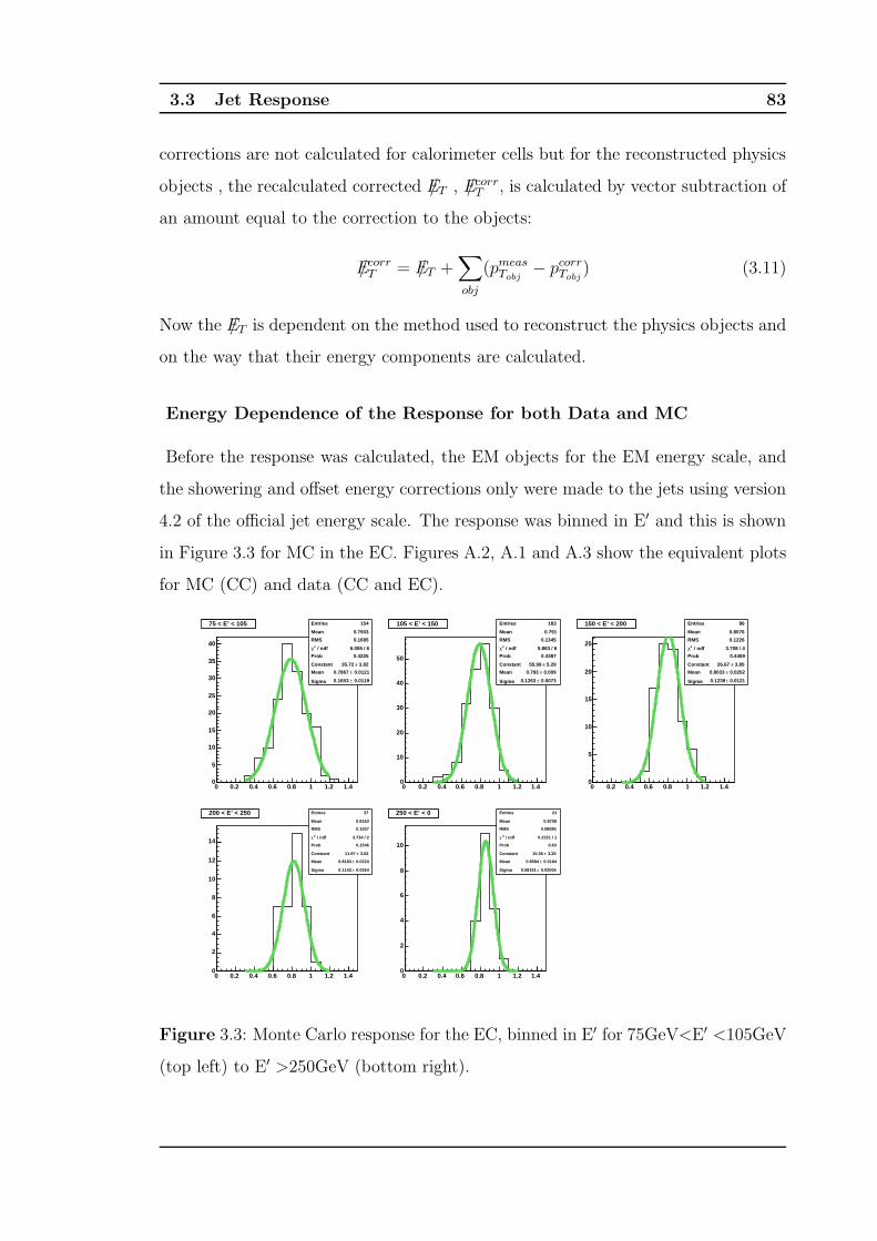
3.3 Jet Response 83
corrections are not calculated for calorimeter cells but for the reconstructed physics
objects , the recalculated corrected E/T , E/corrT , is calculated by vector subtraction of
an amount equal to the correction to the objects:
E/corrT = E/T +
∑
obj
(pmeasTobj
− pcorrTobj
) (3.11)
Now the E/T is dependent on the method used to reconstruct the physics objects and
on the way that their energy components are calculated.
Energy Dependence of the Response for both Data and MC
Before the response was calculated, the EM objects for the EM energy scale, and
the showering and offset energy corrections only were made to the jets using version
4.2 of the official jet energy scale. The response was binned in E′ and this is shown
in Figure 3.3 for MC in the EC. Figures A.2, A.1 and A.3 show the equivalent plots
for MC (CC) and data (CC and EC).
0 0.2 0.4 0.6 0.8 1 1.2 1.40
5
10
15
20
25
30
35
40
75 < E’ < 105 Entries 154
Mean 0.7903
RMS 0.1685
/ ndf 2χ 6.006 / 6
Prob 0.4225
Constant 3.82± 35.72
Mean 0.0121± 0.7867
Sigma 0.0119± 0.1653
75 < E’ < 105
0 0.2 0.4 0.6 0.8 1 1.2 1.40
10
20
30
40
50
105 < E’ < 150 Entries 183
Mean 0.791
RMS 0.1345
/ ndf 2χ 5.863 / 6
Prob 0.4387
Constant 5.29± 55.99
Mean 0.009± 0.793
Sigma 0.0073± 0.1263
105 < E’ < 150
0 0.2 0.4 0.6 0.8 1 1.2 1.40
5
10
15
20
25
150 < E’ < 200 Entries 86
Mean 0.8076
RMS 0.1226
/ ndf 2χ 3.708 / 4
Prob 0.4469
Constant 3.85± 26.67
Mean 0.0202± 0.8033
Sigma 0.0121± 0.1239
150 < E’ < 200
0 0.2 0.4 0.6 0.8 1 1.2 1.40
2
4
6
8
10
12
14
200 < E’ < 250 Entries 37
Mean 0.8163
RMS 0.1027
/ ndf 2χ 3.734 / 2
Prob 0.1546
Constant 3.02± 11.97
Mean 0.0224± 0.8183
Sigma 0.0264± 0.1143
200 < E’ < 250
0 0.2 0.4 0.6 0.8 1 1.2 1.40
2
4
6
8
10
250 < E’ < 0 Entries 21
Mean 0.8708
RMS 0.08086
/ ndf 2χ 0.2321 / 1
Prob 0.63
Constant 3.20± 10.36
Mean 0.0184± 0.8594
Sigma 0.02006± 0.08151
250 < E’ < 0
Figure 3.3: Monte Carlo response for the EC, binned in E′ for 75GeV<E′ <105GeV
(top left) to E′ >250GeV (bottom right).
3.3 Jet Response 84
The response histograms were fitted with Gaussian functions, the mean and
sigma of each fit giving the Rjet and the error on Rjet respectively. Using the
appropriate E ′ − Ejet mapping (Figures 3.2(a) and 3.2(b)), the average response is
mapped to E, and plotted against both E ′ and Ejet in Figures 3.4(a) and 3.4(b).
There is a low-ET bias that can be seen in the curve at low E′ of the E-E′ mapping
in the CC in all response plots and this is discussed later in this section. A quadratic
logarithmic function of the following form is fitted to the response:
Rjet = a + b log(Edet
E0) + c log2(
Edet
E0) (3.12)
This form was used in Run I and is motivated by consideration for the variation of
the particle content of jets with energy.
E’ (GeV)0 50 100 150 200 250 300
jet
R
0.5
0.6
0.7
0.8
0.9
1
1.1
a) Response for CC and EC vs E’, without cryostat factor
CC
EC
a) Response for CC and EC vs E’, without cryostat factor
E’ (GeV)0 50 100 150 200 250 300
jet
R
0.5
0.6
0.7
0.8
0.9
1
1.1
b) Response for CC and EC vs E, without cryostat factor
CC
EC
b) Response for CC and EC vs E, without cryostat factor
(a) Data
E’ (GeV)0 50 100 150 200 250 300
jet
R
0.5
0.6
0.7
0.8
0.9
1
1.1
a) Response for CC and EC vs E’, without cryostat factor
CC
EC
a) Response for CC and EC vs E’, without cryostat factor
E (GeV)0 50 100 150 200 250 300
jet
R
0.5
0.6
0.7
0.8
0.9
1
1.1
b) Response for CC and EC vs E, without cryostat factor
CC
EC
b) Response for CC and EC vs E, without cryostat factor
(b) Monte Carlo
Figure 3.4: Response (∆φ ≥ 3.0) with a quadratic log fit as motivated in the text,
before cryostat factor correction against a) E′(upper) and b) E (lower)
It can be seen that the response to jets is different in the CC and the EC, with a
large variation over the ICR (corresponding to the overlap region). In order that the
binned response histograms in the CC may be combined with the binned response
histograms in the EC, a cryostat factor is calculated to scale the EC response to
that of the CC.
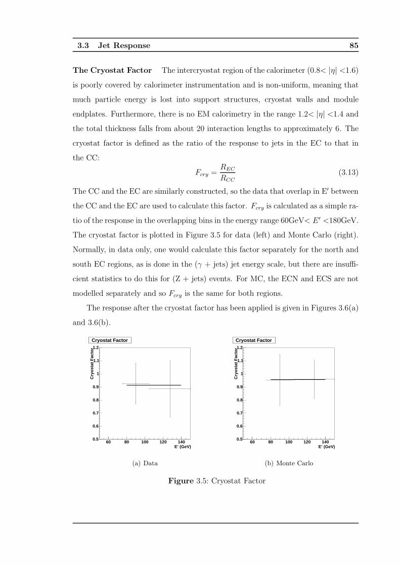
3.3 Jet Response 85
The Cryostat Factor The intercryostat region of the calorimeter (0.8< |η| <1.6)
is poorly covered by calorimeter instrumentation and is non-uniform, meaning that
much particle energy is lost into support structures, cryostat walls and module
endplates. Furthermore, there is no EM calorimetry in the range 1.2< |η| <1.4 and
the total thickness falls from about 20 interaction lengths to approximately 6. The
cryostat factor is defined as the ratio of the response to jets in the EC to that in
the CC:
Fcry =REC
RCC
(3.13)
The CC and the EC are similarly constructed, so the data that overlap in E′ between
the CC and the EC are used to calculate this factor. Fcry is calculated as a simple ra-
tio of the response in the overlapping bins in the energy range 60GeV< E′ <180GeV.
The cryostat factor is plotted in Figure 3.5 for data (left) and Monte Carlo (right).
Normally, in data only, one would calculate this factor separately for the north and
south EC regions, as is done in the (γ + jets) jet energy scale, but there are insuffi-
cient statistics to do this for (Z + jets) events. For MC, the ECN and ECS are not
modelled separately and so Fcry is the same for both regions.
The response after the cryostat factor has been applied is given in Figures 3.6(a)
and 3.6(b).
E’ (GeV)60 80 100 120 140
Cry
ost
at F
acto
r
0.5
0.6
0.7
0.8
0.9
1
1.1
1.2
Cryostat FactorCryostat Factor
(a) Data
E’ (GeV)60 80 100 120 140
Cry
ost
at F
acto
r
0.5
0.6
0.7
0.8
0.9
1
1.1
1.2
Cryostat FactorCryostat Factor
(b) Monte Carlo
Figure 3.5: Cryostat Factor
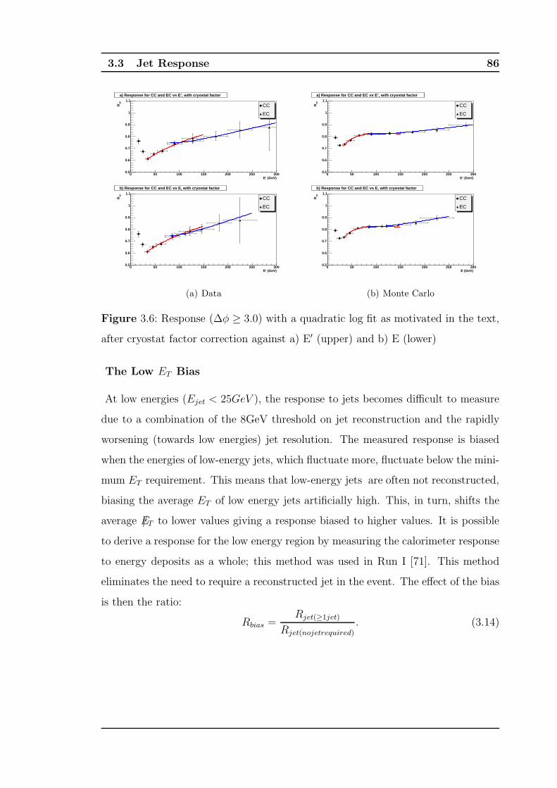
3.3 Jet Response 86
E’ (GeV)0 50 100 150 200 250 300
jet
R
0.5
0.6
0.7
0.8
0.9
1
1.1
a) Response for CC and EC vs E’, with cryostat factor
CC
EC
a) Response for CC and EC vs E’, with cryostat factor
E’ (GeV)0 50 100 150 200 250 300
jet
R
0.5
0.6
0.7
0.8
0.9
1
1.1
b) Response for CC and EC vs E, with cryostat factor
CC
EC
b) Response for CC and EC vs E, with cryostat factor
(a) Data
E’ (GeV)0 50 100 150 200 250 300
jet
R
0.5
0.6
0.7
0.8
0.9
1
1.1
a) Response for CC and EC vs E’, with cryostat factor
CC
EC
a) Response for CC and EC vs E’, with cryostat factor
E (GeV)0 50 100 150 200 250 300
jet
R
0.5
0.6
0.7
0.8
0.9
1
1.1
b) Response for CC and EC vs E, with cryostat factor
CC
EC
b) Response for CC and EC vs E, with cryostat factor
(b) Monte Carlo
Figure 3.6: Response (∆φ ≥ 3.0) with a quadratic log fit as motivated in the text,
after cryostat factor correction against a) E′ (upper) and b) E (lower)
The Low ET Bias
At low energies (Ejet < 25GeV ), the response to jets becomes difficult to measure
due to a combination of the 8GeV threshold on jet reconstruction and the rapidly
worsening (towards low energies) jet resolution. The measured response is biased
when the energies of low-energy jets, which fluctuate more, fluctuate below the mini-
mum ET requirement. This means that low-energy jets are often not reconstructed,
biasing the average ET of low energy jets artificially high. This, in turn, shifts the
average E/T to lower values giving a response biased to higher values. It is possible
to derive a response for the low energy region by measuring the calorimeter response
to energy deposits as a whole; this method was used in Run I [71]. This method
eliminates the need to require a reconstructed jet in the event. The effect of the bias
is then the ratio:
Rbias =Rjet(≥1jet)
Rjet(nojetrequired)
. (3.14)
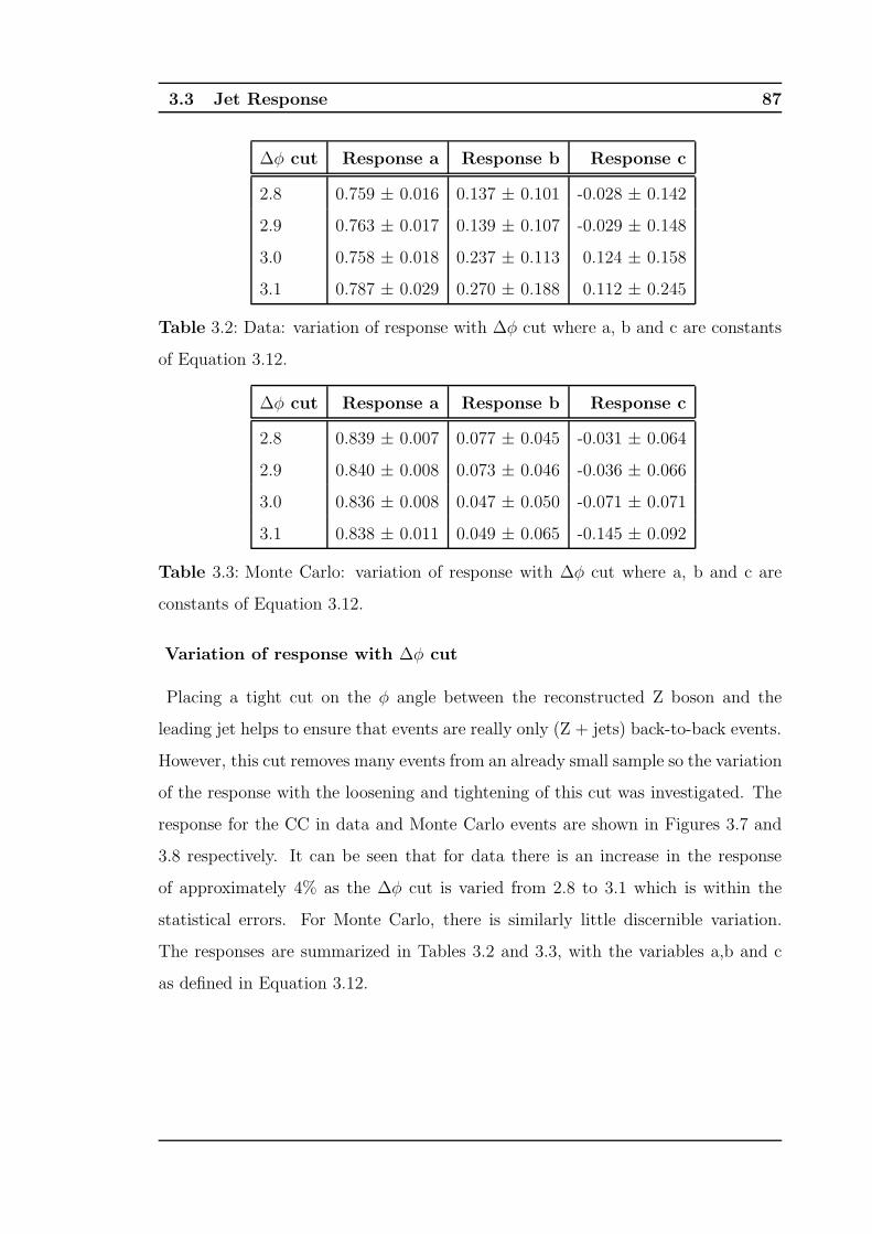
3.3 Jet Response 87
∆φ cut Response a Response b Response c
2.8 0.759 ± 0.016 0.137 ± 0.101 -0.028 ± 0.142
2.9 0.763 ± 0.017 0.139 ± 0.107 -0.029 ± 0.148
3.0 0.758 ± 0.018 0.237 ± 0.113 0.124 ± 0.158
3.1 0.787 ± 0.029 0.270 ± 0.188 0.112 ± 0.245
Table 3.2: Data: variation of response with ∆φ cut where a, b and c are constants
of Equation 3.12.
∆φ cut Response a Response b Response c
2.8 0.839 ± 0.007 0.077 ± 0.045 -0.031 ± 0.064
2.9 0.840 ± 0.008 0.073 ± 0.046 -0.036 ± 0.066
3.0 0.836 ± 0.008 0.047 ± 0.050 -0.071 ± 0.071
3.1 0.838 ± 0.011 0.049 ± 0.065 -0.145 ± 0.092
Table 3.3: Monte Carlo: variation of response with ∆φ cut where a, b and c are
constants of Equation 3.12.
Variation of response with ∆φ cut
Placing a tight cut on the φ angle between the reconstructed Z boson and the
leading jet helps to ensure that events are really only (Z + jets) back-to-back events.
However, this cut removes many events from an already small sample so the variation
of the response with the loosening and tightening of this cut was investigated. The
response for the CC in data and Monte Carlo events are shown in Figures 3.7 and
3.8 respectively. It can be seen that for data there is an increase in the response
of approximately 4% as the ∆φ cut is varied from 2.8 to 3.1 which is within the
statistical errors. For Monte Carlo, there is similarly little discernible variation.
The responses are summarized in Tables 3.2 and 3.3, with the variables a,b and c
as defined in Equation 3.12.
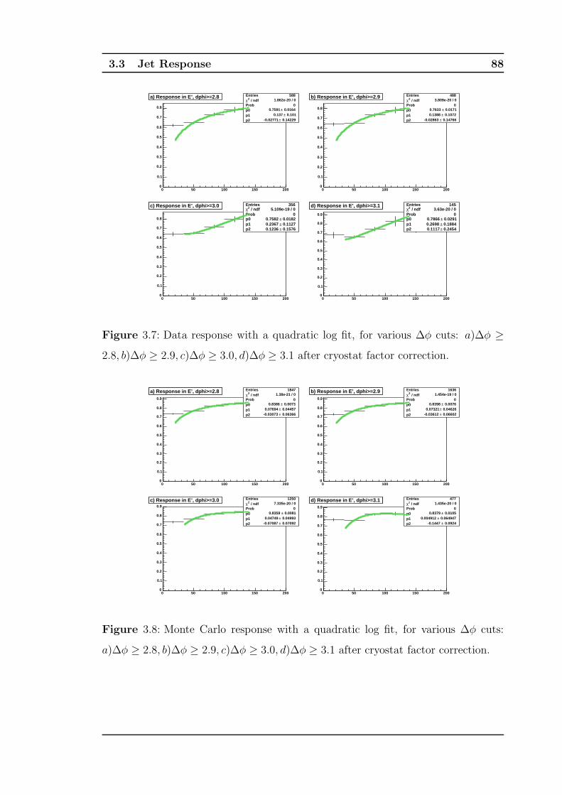
3.3 Jet Response 88
0 50 100 150 2000
0.1
0.2
0.3
0.4
0.5
0.6
0.7
0.8
a) Response in E’, dphi>=2.8 Entries 588 / ndf 2χ 1.862e-20 / 0
Prob 0p0 0.0164± 0.7591
p1 0.101± 0.137
p2 0.14229± -0.02771
a) Response in E’, dphi>=2.8
0 50 100 150 2000
0.1
0.2
0.3
0.4
0.5
0.6
0.7
0.8
b) Response in E’, dphi>=2.9 Entries 488 / ndf 2χ 3.809e-20 / 0
Prob 0p0 0.0171± 0.7633
p1 0.1072± 0.1388
p2 0.14766± -0.02863
b) Response in E’, dphi>=2.9
0 50 100 150 2000
0.1
0.2
0.3
0.4
0.5
0.6
0.7
0.8
c) Response in E’, dphi>=3.0 Entries 356 / ndf 2χ 5.109e-19 / 0
Prob 0p0 0.0182± 0.7582 p1 0.1127± 0.2367 p2 0.1576± 0.1236
c) Response in E’, dphi>=3.0
0 50 100 150 2000
0.1
0.2
0.3
0.4
0.5
0.6
0.7
0.8
0.9
d) Response in E’, dphi>=3.1 Entries 145 / ndf 2χ 3.63e-20 / 0
Prob 0p0 0.0291± 0.7866 p1 0.1884± 0.2698 p2 0.2454± 0.1117
d) Response in E’, dphi>=3.1
Figure 3.7: Data response with a quadratic log fit, for various ∆φ cuts: a)∆φ ≥2.8, b)∆φ ≥ 2.9, c)∆φ ≥ 3.0, d)∆φ ≥ 3.1 after cryostat factor correction.
0 50 100 150 2000
0.1
0.2
0.3
0.4
0.5
0.6
0.7
0.8
0.9
a) Response in E’, dphi>=2.8 Entries 1847 / ndf 2χ 1.38e-21 / 0
Prob 0p0 0.0073± 0.8386
p1 0.04457± 0.07694
p2 0.06366± -0.03073
a) Response in E’, dphi>=2.8
0 50 100 150 2000
0.1
0.2
0.3
0.4
0.5
0.6
0.7
0.8
0.9
b) Response in E’, dphi>=2.9 Entries 1636 / ndf 2χ 1.454e-19 / 0
Prob 0p0 0.0076± 0.8398
p1 0.04626± 0.07321
p2 0.06602± -0.03612
b) Response in E’, dphi>=2.9
0 50 100 150 2000
0.1
0.2
0.3
0.4
0.5
0.6
0.7
0.8
0.9
c) Response in E’, dphi>=3.0 Entries 1250 / ndf 2χ 7.335e-20 / 0
Prob 0p0 0.0081± 0.8359
p1 0.04993± 0.04749
p2 0.07092± -0.07087
c) Response in E’, dphi>=3.0
0 50 100 150 2000
0.1
0.2
0.3
0.4
0.5
0.6
0.7
0.8
0.9
d) Response in E’, dphi>=3.1 Entries 477 / ndf 2χ 1.435e-20 / 0
Prob 0p0 0.0105± 0.8379
p1 0.064947± 0.004912
p2 0.0924± -0.1447
d) Response in E’, dphi>=3.1
Figure 3.8: Monte Carlo response with a quadratic log fit, for various ∆φ cuts:
a)∆φ ≥ 2.8, b)∆φ ≥ 2.9, c)∆φ ≥ 3.0, d)∆φ ≥ 3.1 after cryostat factor correction.
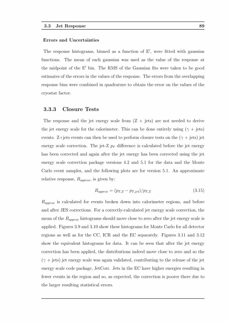
3.3 Jet Response 89
Errors and Uncertainties
The response histograms, binned as a function of E′, were fitted with gaussian
functions. The mean of each gaussian was used as the value of the response at
the midpoint of the E′ bin. The RMS of the Gaussian fits were taken to be good
estimates of the errors in the values of the response. The errors from the overlapping
response bins were combined in quadrature to obtain the error on the values of the
cryostat factor.
3.3.3 Closure Tests
The response and the jet energy scale from (Z + jets) are not needed to derive
the jet energy scale for the calorimeter. This can be done entirely using (γ + jets)
events. Z+jets events can then be used to perform closure tests on the (γ + jets) jet
energy scale correction. The jet-Z pT difference is calculated before the jet energy
has been corrected and again after the jet energy has been corrected using the jet
energy scale correction package versions 4.2 and 5.1 for the data and the Monte
Carlo event samples, and the following plots are for version 5.1. An approximate
relative response, Rapprox, is given by:
Rapprox = (pT,Z − pT,jet)/pT,Z (3.15)
Rapprox is calculated for events broken down into calorimeter regions, and before
and after JES corrections. For a correctly-calculated jet energy scale correction, the
mean of the Rapprox histograms should move close to zero after the jet energy scale is
applied. Figures 3.9 and 3.10 show these histograms for Monte Carlo for all detector
regions as well as for the CC, ICR and the EC separately. Figures 3.11 and 3.12
show the equivalent histograms for data. It can be seen that after the jet energy
correction has been applied, the distributions indeed move close to zero and so the
(γ + jets) jet energy scale was again validated, contributing to the release of the jet
energy scale code package, JetCorr. Jets in the EC have higher energies resulting in
fewer events in the region and so, as expected, the correction is poorer there due to
the larger resulting statistical errors.
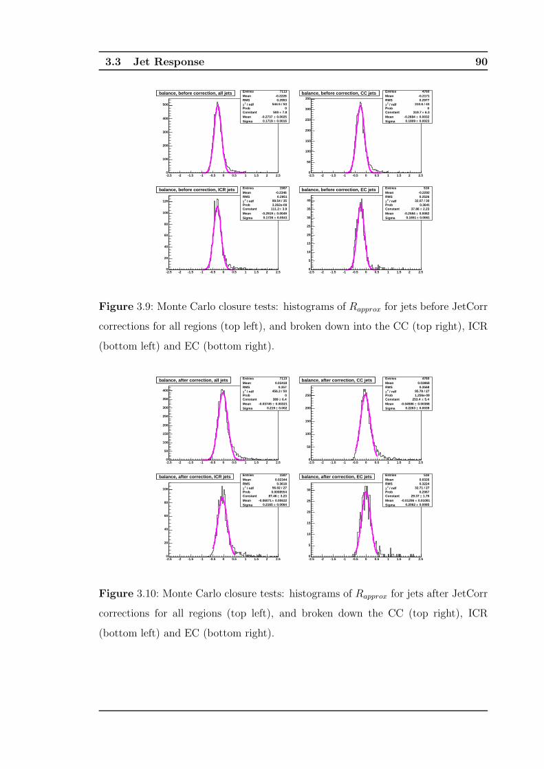
3.3 Jet Response 90
-2.5 -2 -1.5 -1 -0.5 0 0.5 1 1.5 2 2.50
100
200
300
400
500
balance, before correction, all jets Entries 7113Mean -0.2228RMS 0.2953
/ ndf 2χ 544.5 / 53Prob 0Constant 7.8± 500 Mean 0.0025± -0.2737 Sigma 0.0016± 0.1719
balance, before correction, all jets
-2.5 -2 -1.5 -1 -0.5 0 0.5 1 1.5 2 2.50
50
100
150
200
250
300
350
balance, before correction, CC jets Entries 4760Mean -0.2171RMS 0.2977
/ ndf 2χ 310.6 / 43Prob 0Constant 6.3± 319.7 Mean 0.0032± -0.2684 Sigma 0.0023± 0.1809
balance, before correction, CC jets
-2.5 -2 -1.5 -1 -0.5 0 0.5 1 1.5 2 2.50
20
40
60
80
100
120
balance, before correction, ICR jets Entries 1597Mean -0.2346RMS 0.2951
/ ndf 2χ 99.54 / 35Prob 3.262e-09Constant 3.9± 111.2 Mean 0.0049± -0.2919 Sigma 0.0041± 0.1726
balance, before correction, ICR jets
-2.5 -2 -1.5 -1 -0.5 0 0.5 1 1.5 2 2.50
5
10
15
20
25
30
35
40
balance, before correction, EC jets Entries 516Mean -0.2292RMS 0.2526
/ ndf 2χ 32.07 / 30Prob 0.3641Constant 2.23± 37.86 Mean 0.0082± -0.2584 Sigma 0.0061± 0.1651
balance, before correction, EC jets
Figure 3.9: Monte Carlo closure tests: histograms of Rapprox for jets before JetCorr
corrections for all regions (top left), and broken down into the CC (top right), ICR
(bottom left) and EC (bottom right).
-2.5 -2 -1.5 -1 -0.5 0 0.5 1 1.5 2 2.50
50
100
150
200
250
300
350
400
balance, after correction, all jets Entries 7113Mean 0.03418RMS 0.357
/ ndf 2χ 456.3 / 50Prob 0Constant 6.4± 389 Mean 0.00321± -0.03745 Sigma 0.002± 0.219
balance, after correction, all jets
-2.5 -2 -1.5 -1 -0.5 0 0.5 1 1.5 2 2.50
50
100
150
200
250
balance, after correction, CC jets Entries 4760Mean 0.03868RMS 0.3568
/ ndf 2χ 95.78 / 27Prob 1.256e-09Constant 5.4± 253.4 Mean 0.00388± -0.04586 Sigma 0.0039± 0.2263
balance, after correction, CC jets
-2.5 -2 -1.5 -1 -0.5 0 0.5 1 1.5 2 2.50
20
40
60
80
100
balance, after correction, ICR jets Entries 1597Mean 0.02344RMS 0.3618
/ ndf 2χ 56.02 / 27Prob 0.0008554Constant 3.23± 87.46 Mean 0.00632± -0.06071 Sigma 0.0064± 0.2165
balance, after correction, ICR jets
-2.5 -2 -1.5 -1 -0.5 0 0.5 1 1.5 2 2.50
5
10
15
20
25
30
balance, after correction, EC jets Entries 516Mean 0.0326RMS 0.3224
/ ndf 2χ 32.71 / 27Prob 0.2067Constant 1.76± 29.37 Mean 0.01081± -0.01296 Sigma 0.0085± 0.2062
balance, after correction, EC jets
Figure 3.10: Monte Carlo closure tests: histograms of Rapprox for jets after JetCorr
corrections for all regions (top left), and broken down the CC (top right), ICR
(bottom left) and EC (bottom right).
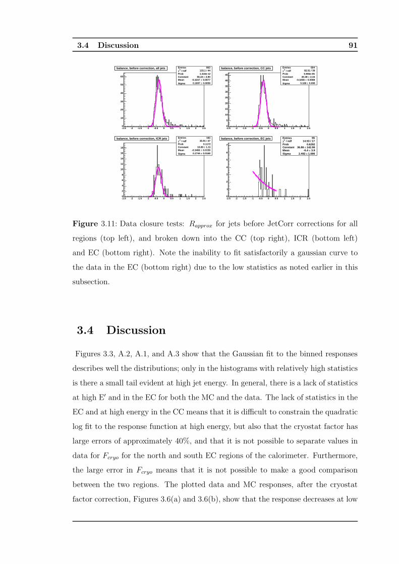
3.4 Discussion 91
-2.5 -2 -1.5 -1 -0.5 0 0.5 1 1.5 2 2.50
10
20
30
40
50
60
balance, before correction, all jets Entries 863 / ndf 2χ 133.1 / 44
Prob 1.418e-12Constant 2.80± 56.22 Mean 0.0077± -0.3237
Sigma 0.0058± 0.1697
balance, before correction, all jets
-2.5 -2 -1.5 -1 -0.5 0 0.5 1 1.5 2 2.50
5
10
15
20
25
30
35
40
45
balance, before correction, CC jets Entries 604 / ndf 2χ 82.51 / 39
Prob 5.906e-05Constant 2.34± 40.48 Mean 0.0088± -0.3258
Sigma 0.006± 0.168
balance, before correction, CC jets
-2.5 -2 -1.5 -1 -0.5 0 0.5 1 1.5 2 2.50
2
4
6
8
10
12
14
16
18
balance, before correction, ICR jets Entries 183 / ndf 2χ 35.91 / 27
Prob 0.1172Constant 1.31± 10.89 Mean 0.0159± -0.3466
Sigma 0.0168± 0.1744
balance, before correction, ICR jets
-2.5 -2 -1.5 -1 -0.5 0 0.5 1 1.5 2 2.50
1
2
3
4
5
6
7
balance, before correction, EC jets Entries 55 / ndf 2χ 14.53 / 17
Prob 0.6292Constant 142.96± 36.86 Mean 3.9± -6.4 Sigma 1.686± 2.492
balance, before correction, EC jets
Figure 3.11: Data closure tests: Rapprox for jets before JetCorr corrections for all
regions (top left), and broken down into the CC (top right), ICR (bottom left)
and EC (bottom right). Note the inability to fit satisfactorily a gaussian curve to
the data in the EC (bottom right) due to the low statistics as noted earlier in this
subsection.
3.4 Discussion
Figures 3.3, A.2, A.1, and A.3 show that the Gaussian fit to the binned responses
describes well the distributions; only in the histograms with relatively high statistics
is there a small tail evident at high jet energy. In general, there is a lack of statistics
at high E′ and in the EC for both the MC and the data. The lack of statistics in the
EC and at high energy in the CC means that it is difficult to constrain the quadratic
log fit to the response function at high energy, but also that the cryostat factor has
large errors of approximately 40%, and that it is not possible to separate values in
data for Fcryo for the north and south EC regions of the calorimeter. Furthermore,
the large error in Fcryo means that it is not possible to make a good comparison
between the two regions. The plotted data and MC responses, after the cryostat
factor correction, Figures 3.6(a) and 3.6(b), show that the response decreases at low
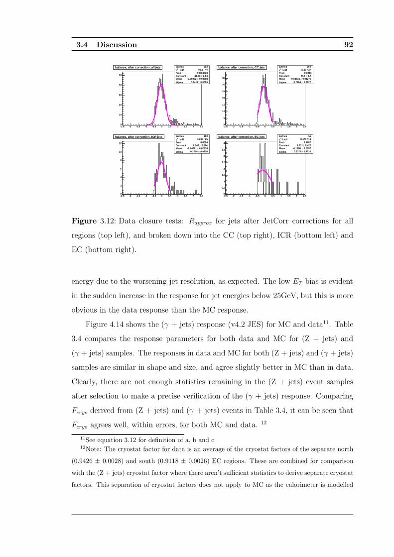
3.4 Discussion 92
-2.5 -2 -1.5 -1 -0.5 0 0.5 1 1.5 2 2.50
10
20
30
40
50
balance, after correction, all jets Entries 863 / ndf 2χ 82.1 / 44
Prob 0.0004323Constant 2.04± 41.23 Mean 0.00988± -0.05032
Sigma 0.0085± 0.2411
balance, after correction, all jets
-2.5 -2 -1.5 -1 -0.5 0 0.5 1 1.5 2 2.50
5
10
15
20
25
30
35
balance, after correction, CC jets Entries 604 / ndf 2χ 30.29 / 27
Prob 0.3011Constant 1.7± 29.1 Mean 0.01275± -0.08631
Sigma 0.0127± 0.2484
balance, after correction, CC jets
-2.5 -2 -1.5 -1 -0.5 0 0.5 1 1.5 2 2.50
2
4
6
8
10
12
balance, after correction, ICR jets Entries 183 / ndf 2χ 16.98 / 25
Prob 0.8824Constant 0.874± 7.646 Mean 0.02939± -0.04781
Sigma 0.0326± 0.2714
balance, after correction, ICR jets
-2.5 -2 -1.5 -1 -0.5 0 0.5 1 1.5 2 2.50
0.5
1
1.5
2
2.5
3
3.5
4
balance, after correction, EC jets Entries 55 / ndf 2χ 8.475 / 18
Prob 0.9707Constant 0.422± 1.911 Mean 0.2857± -0.1868
Sigma 0.4532± 0.5371
balance, after correction, EC jets
Figure 3.12: Data closure tests: Rapprox for jets after JetCorr corrections for all
regions (top left), and broken down into the CC (top right), ICR (bottom left) and
EC (bottom right).
energy due to the worsening jet resolution, as expected. The low ET bias is evident
in the sudden increase in the response for jet energies below 25GeV, but this is more
obvious in the data response than the MC response.
Figure 4.14 shows the (γ + jets) response (v4.2 JES) for MC and data11. Table
3.4 compares the response parameters for both data and MC for (Z + jets) and
(γ + jets) samples. The responses in data and MC for both (Z + jets) and (γ + jets)
samples are similar in shape and size, and agree slightly better in MC than in data.
Clearly, there are not enough statistics remaining in the (Z + jets) event samples
after selection to make a precise verification of the (γ + jets) response. Comparing
Fcryo derived from (Z + jets) and (γ + jets) events in Table 3.4, it can be seen that
Fcryo agrees well, within errors, for both MC and data. 12
11See equation 3.12 for definition of a, b and c12Note: The cryostat factor for data is an average of the cryostat factors of the separate north
(0.9426 ± 0.0028) and south (0.9118 ± 0.0026) EC regions. These are combined for comparison
with the (Z + jets) cryostat factor where there aren’t sufficient statistics to derive separate cryostat
factors. This separation of cryostat factors does not apply to MC as the calorimeter is modelled
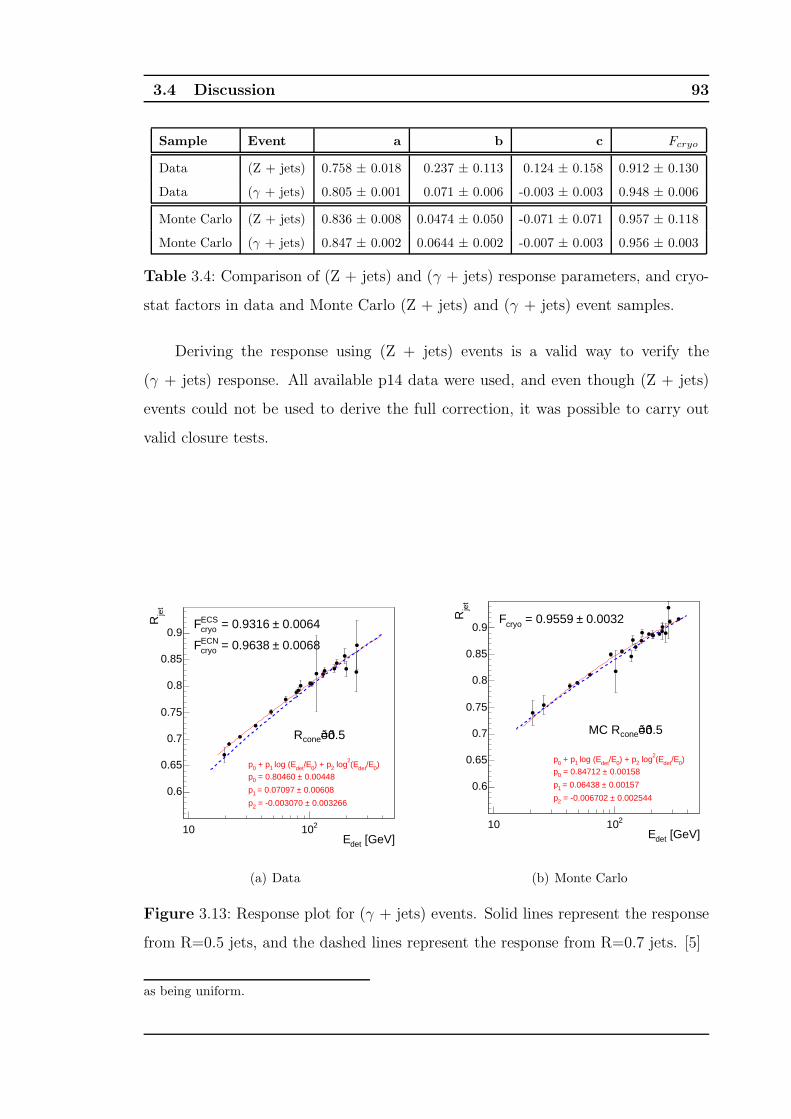
3.4 Discussion 93
Sample Event a b c Fcryo
Data (Z + jets) 0.758 ± 0.018 0.237 ± 0.113 0.124 ± 0.158 0.912 ± 0.130
Data (γ + jets) 0.805 ± 0.001 0.071 ± 0.006 -0.003 ± 0.003 0.948 ± 0.006
Monte Carlo (Z + jets) 0.836 ± 0.008 0.0474 ± 0.050 -0.071 ± 0.071 0.957 ± 0.118
Monte Carlo (γ + jets) 0.847 ± 0.002 0.0644 ± 0.002 -0.007 ± 0.003 0.956 ± 0.003
Table 3.4: Comparison of (Z + jets) and (γ + jets) response parameters, and cryo-
stat factors in data and Monte Carlo (Z + jets) and (γ + jets) event samples.
Deriving the response using (Z + jets) events is a valid way to verify the
(γ + jets) response. All available p14 data were used, and even though (Z + jets)
events could not be used to derive the full correction, it was possible to carry out
valid closure tests.
[GeV]detE10 210
jet
R
0.6
0.65
0.7
0.75
0.8
0.85
0.9
)0/Edet(E2
log2) + p0/Edet log (E1 + p0p
0.00448± = 0.80460 0p
0.00608± = 0.07097 1p
0.003266± = -0.003070 2p
ð=ð0.5cone R
0.0064± = 0.9316 ECScryoF
0.0068± = 0.9638 ECNcryoF
Figure 3.23: Jet response for jets with one size of R = 0:5. Dashed lines represent thejet response obtained for R = 0:7 one.29
(a) Data
Figure 3.31: Jet response for MC jets with one size of R = 0:7. Relative error of the �tin the entral alorimeter (left plot) and the end ap ryostats (right plot).
[GeV]detE10 210
jet
R
0.6
0.65
0.7
0.75
0.8
0.85
0.9
)0/Edet(E2
log2) + p0/Edet log (E1 + p0p
0.00158± = 0.84712 0p
0.00157± = 0.06438 1p
0.002544± = -0.006702 2p
ð=ð0.5coneMC R
0.0032± = 0.9559 cryoF
Figure 3.32: MC jet response as a fun tion of jet energy Edet for jets with one size ofR = 0:5. Dashed line represents MC response in CC for one R = 0:7.36(b) Monte Carlo
Figure 3.13: Response plot for (γ + jets) events. Solid lines represent the response
from R=0.5 jets, and the dashed lines represent the response from R=0.7 jets. [5]
as being uniform.

3.5 Conclusion 94
3.5 Conclusion
As part of the certification of version 4.2 of the (γ + jets) official jet energy response,
the response was calculated for data and MC for p14 (Z + jets) events, using the
missing ET projection fraction method. Closure tests on (Z + jets) events, using
versions 4.2 and 5.1 of the (γ + jets) jet energy scale were performed, contributing to
the release of the jet energy scale. Both the (Z + jets) response and the closure tests
verified the (γ + jets) response, providing a valid check of the response before it was
implemented as part of the jet energy scale at D��O. The (Z + jets) and (γ + jets)
response agreed well within errors and no discernible variation of the (Z + jets)
response with the variation of the back-to-back requirement of the Z boson and
the leading jet was found. Despite using all available data and MC, the lack of
statistics meant that (Z + jets) events could not be used to derive the full jet energy
correction or be used for a precision verification of the (γ + jets) response. However,
approximately 1fb−1 data are now available for use with a new collaboration-wide
analysis format; it is now possible to derive a response for (Z + jets) events with a
precision comparable to the (γ + jets) response.

4 The Calorimeter Response to Semileptonic Decays and Energy Flow95
Chapter 4
The Calorimeter Response to
Semileptonic Decays and Energy
Flow
4.1 Introduction
Many physics processes of interest at DØ involve b-jets. For example, one of the
best ways to detect a light, standard model Higgs boson is via its decay to a bb pair;
DØ has a large b-physics programme, but many other physics programmes involve
b-jets. Therefore, it is important that DØ has both a good jet energy scale that is
appropriate to its physics programmes, and that it improves the jet energy resolution
using all available techniques. In the first part of this chapter, an improvement to
the jet energy scale is calculated specifically for certain commonly-used b-jets. In
the second part of this chapter, an electromagnetic scale for calorimeter clusters
is derived as part of the implementation of a new algorithm to improve jet energy
resolution using the tracking system together with the calorimeter.
B-jets have different characteristics to light quark jets since mb ≫ mq; b-jets
have different decay kinematics and harder fragmentation leading to a different jet
energy scale. Approximately 10% of the time [8] the b-jet contains a lepton and
4.1 Introduction 96
a neutrino from the direct semileptonic decay of the original B–hadron (b → lν).
Alternatively, the B–hadron may decay via a charm-hadron, and then the c-quark
itself may decay semileptonically approximately 20% of the time [8], this process is
denoted as a cascade decay (b → c → lν). In both cascade and direct decays the
measured jet energy will not include the energy of the escaping neutrino, but will
include the energy of the lepton depending on whether it is an electron or a muon. If
the lepton is an electron, all its energy will be contained within the calorimeter, but,
for a muon, only a small amount of energy is deposited (typically on the order of 2
GeV). Thus for semileptonic decays, the energy of the b-jet has to be corrected for
the energy of the neutrino, and for muonic semileptonic decays, the muon energy
measured in the muon detector must also be added back into the jet energy. A
correction may be made as part of the jet energy scale for the special case of muonic
semileptonic decays. A scalar, Monte Carlo based, semileptonic correction to b-jets
is derived in the first part of this chapter using tt events, and this was incorporated
into versions 5.1 and 5.3 of the DØ JES [70]. The v5.1 corrections use p14 data
and Monte Carlo. In this chapter, the muonic semileptonic correction is addressed,
as part of the official jet energy scale version 5.1. A vector semileptonic correction
is also considered. The effects of the semileptonic correction on the dijet mass
resolution in Z → bb and H → bb MC events are evaluated.
At D��O, it is possible to improve the jet energy resolution and reduce the sys-
tematic error of jet energy measurements by combining the energy measured by the
calorimeter with the momentum measured in the tracking system. Since the tracker
has better momentum resolution than the calorimeter at low energy, it may be used
to compensate for the poor low-energy measurements of the calorimeter. The energy
flow (eflow) algorithm [77] reconstructs the flow of energy in an event, combining
information from the subdetectors to create eflow particles from tracks in the tracker
through to calorimeter cells. These well-understood eflow particles are used to re-
construct more complex physics objects such as jets, and event properties. In this
chapter, as a necessary part of the possible implementation of an eflow algorithm, an
electromagnetic scale is derived for calorimeter cell clusters, using low-momentum
tracks.
4.2 Semileptonic Decays: Muons 97
4.2 Semileptonic Decays: Muons
4.2.1 Definition of the Semileptonic Correction
To measure correctly the jet energy for muonic b-jets, a correction must be calculated
to compensate for the undetectable neutrino but this is not straightforward. In
addition, the muon energy must be added to the jet energy. The muonic semileptonic
correction is derived for direct and cascade decays using the method prescribed
originally in the p13 certification of the jet energy scale [78]. The correction factor
is defined as:
C =EMC
µ + EMCν
Emeasµ
(4.1)
where EMCµ and EMC
ν refer to the generator-level muon and neutrino energies re-
spectively, and Emeasµ to the reconstructed energy of the muon. The correction factor
was parameterised as a function of the reconstructed muon energy. A second-order
dependence of the correction on the b-jet energy and on prelT was also investigated,
where prelT is the pT of the muon with respect to the combined muon-b-jet axis. The
prelT can be a powerful discriminator of b-jets from charm and light jets [79]. A fit
to the correction factor using the functional form in Equation 4.2 was made.
Cfit = p0 + e(p1+p2·Emeasµ ) (4.2)
Event Selection
The event selection is divided into three main parts in addition to general event cuts:
the generator level selection, the reconstructed jet selection and the reconstructed
muon selection. The correction factor is derived from 88,000, p14.02.00, Pythia-
generated [74] plate1 tt → Wb(lν)Wb(lν) Monte Carlo events, corrected with v.5.1
of the official DØ jet energy scale.
General Event Cuts As in the derivation of the jet response, it was required
that the primary vertex z-coordinate must have |z| <50cm and that the primary
vertex must have at least two associated tracks.
1Plate MC events are those where the calorimeter has been simulated as a series of uranium
and argon plates.

4.2 Semileptonic Decays: Muons 98
Generator-Level Selection Cuts The selection at the generator level aimed
to identify events in which either of the two b-jets contained a semileptonic decay,
either direct or cascade. The generator level selection consisted of the following
steps:
1. b-quarks from the decay of the top were selected and their decay chains
inspected to see if they contained an oppositely signed muon and a neutrino,
originating from the same generator level vertex.
2. If the parent of the muon and neutrino was a B-meson then the decay was
flagged as direct.
3. If the parent was a C-meson and the parent of the C-meson was a B-meson
then the decay was flagged as cascade.
4. If one or both b-quarks from the top quarks satisfied the above requirements
the event was passed.
The above selection allowed the unambiguous identification of events containing
semileptonic decays of interest and the unambiguous selection of the generator level
muon, neutrino and b-quark. In the case of both b-quarks decaying semileptonically,
the two decays were treated independently and hence event rejection should be
understood in terms of either decay.
Muon Selection Reconstructed muons passing the medium identification (good
muons) requirements as defined in Section 2.2.8 were used. If the △R in η×φ space
between the generator-level and reconstructed muons was less than 0.2 then they
were considered matched. If more than one reconstructed muon was matched to the
same generator-level muon, the event was rejected.
Jet Selection The jets were reconstructed using the Run II cone algorithm with
a cone size of 0.5. The jets were selected using the standard jet-ID for p14, as used
in the (Z + jets) response event selection. The jet was matched to the b-jet by
requiring that the △R between the jet and the b-quark was less than the 0.5 (the
cone size of the jet). If it was possible to match more than one jet to the b-quark,
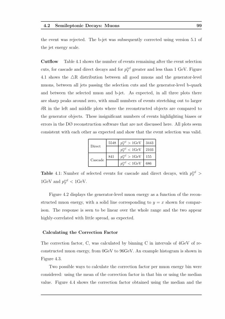
4.2 Semileptonic Decays: Muons 99
the event was rejected. The b-jet was subsequently corrected using version 5.1 of
the jet energy scale.
Cutflow Table 4.1 shows the number of events remaining after the event selection
cuts, for cascade and direct decays and for prelT greater and less than 1 GeV. Figure
4.1 shows the △R distribution between all good muons and the generator-level
muons, between all jets passing the selection cuts and the generator-level b-quark
and between the selected muon and b-jet. As expected, in all three plots there
are sharp peaks around zero, with small numbers of events stretching out to larger
δR in the left and middle plots where the reconstructed objects are compared to
the generator objects. These insignificant numbers of events highlighting biases or
errors in the DØ reconstruction software that are not discussed here. All plots seem
consistent with each other as expected and show that the event selection was valid.
Direct5548 prel
T > 1GeV 3443
prelT < 1GeV 2103
Cascade841 prel
T > 1GeV 155
prelT < 1GeV 686
Table 4.1: Number of selected events for cascade and direct decays, with prelT >
1GeV and prelT < 1GeV.
Figure 4.2 displays the generator-level muon energy as a function of the recon-
structed muon energy, with a solid line corresponding to y = x shown for compar-
ison. The response is seen to be linear over the whole range and the two appear
highly-correlated with little spread, as expected.
Calculating the Correction Factor
The correction factor, C, was calculated by binning C in intervals of 4GeV of re-
constructed muon energy, from 0GeV to 96GeV. An example histogram is shown in
Figure 4.3.
Two possible ways to calculate the correction factor per muon energy bin were
considered: using the mean of the correction factor in that bin or using the median
value. Figure 4.4 shows the correction factor obtained using the median and the
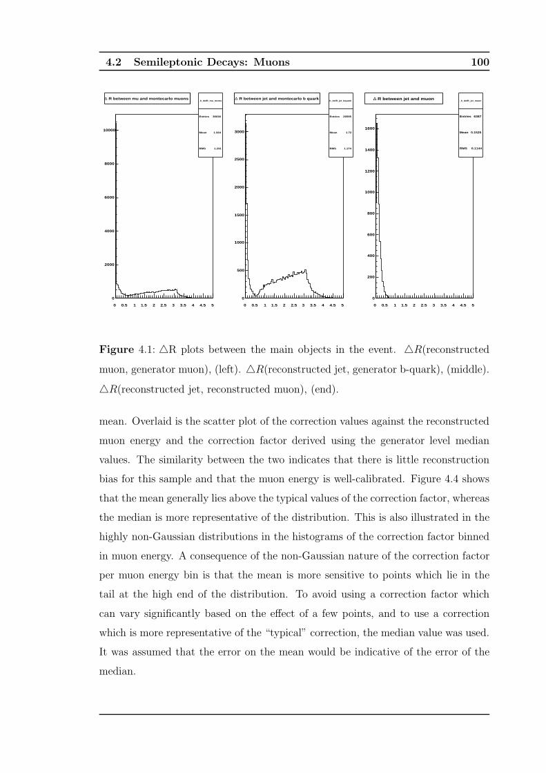
4.2 Semileptonic Decays: Muons 100
0 0.5 1 1.5 2 2.5 3 3.5 4 4.5 5
0
2000
4000
6000
8000
10000
R between mu and montecarlo muons ∆ _h_delR_mu_mcmu
Entries 36036
Mean 1.334
RMS 1.231
R between mu and montecarlo muons ∆
0 0.5 1 1.5 2 2.5 3 3.5 4 4.5 5
0
500
1000
1500
2000
2500
3000
R between jet and montecarlo b quark ∆ _h_delR_jet_bquark
Entries 26595
Mean 1.72
RMS 1.174
R between jet and montecarlo b quark ∆
0 0.5 1 1.5 2 2.5 3 3.5 4 4.5 5
0
200
400
600
800
1000
1200
1400
1600
R between jet and muon ∆ _h_delR_jet_muon
Entries 6387
Mean 0.1525
RMS 0.1144
R between jet and muon ∆
Figure 4.1: △R plots between the main objects in the event. △R(reconstructed
muon, generator muon), (left). △R(reconstructed jet, generator b-quark), (middle).
△R(reconstructed jet, reconstructed muon), (end).
mean. Overlaid is the scatter plot of the correction values against the reconstructed
muon energy and the correction factor derived using the generator level median
values. The similarity between the two indicates that there is little reconstruction
bias for this sample and that the muon energy is well-calibrated. Figure 4.4 shows
that the mean generally lies above the typical values of the correction factor, whereas
the median is more representative of the distribution. This is also illustrated in the
highly non-Gaussian distributions in the histograms of the correction factor binned
in muon energy. A consequence of the non-Gaussian nature of the correction factor
per muon energy bin is that the mean is more sensitive to points which lie in the
tail at the high end of the distribution. To avoid using a correction factor which
can vary significantly based on the effect of a few points, and to use a correction
which is more representative of the “typical” correction, the median value was used.
It was assumed that the error on the mean would be indicative of the error of the
median.
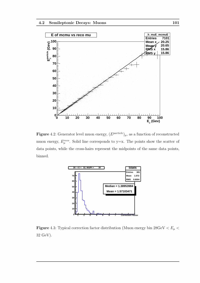
4.2 Semileptonic Decays: Muons 101
(Gev)µE0 10 20 30 40 50 60 70 80 90 100
(G
ev)
µpar
ticl
eE
0
10
20
30
40
50
60
70
80
90
100
E of mcmu vs reco mu _h_muE_mcmuEEntries 7101Mean x 20.25Mean y 20.65RMS x 15.86RMS y 15.86
E of mcmu vs reco mu
Figure 4.2: Generator level muon energy, (Eparticle)µ, as a function of reconstructed
muon energy, Erecoµ . Solid line corresponds to y=x. The points show the scatter of
data points, while the cross-hairs represent the midpoints of the same data points,
binned.
1 2 3 4 5 6 7 Correction Factor0
10
20
30
40
50
60
70
28 < E < 32, MidPt = 30 StatsEntries 381
Mean 1.572
RMS 0.6004
Median = 1.38953984
Mean = 1.57103471
28 < E < 32, MidPt = 30
Figure 4.3: Typical correction factor distribution (Muon energy bin 28GeV < Eµ <
32 GeV).
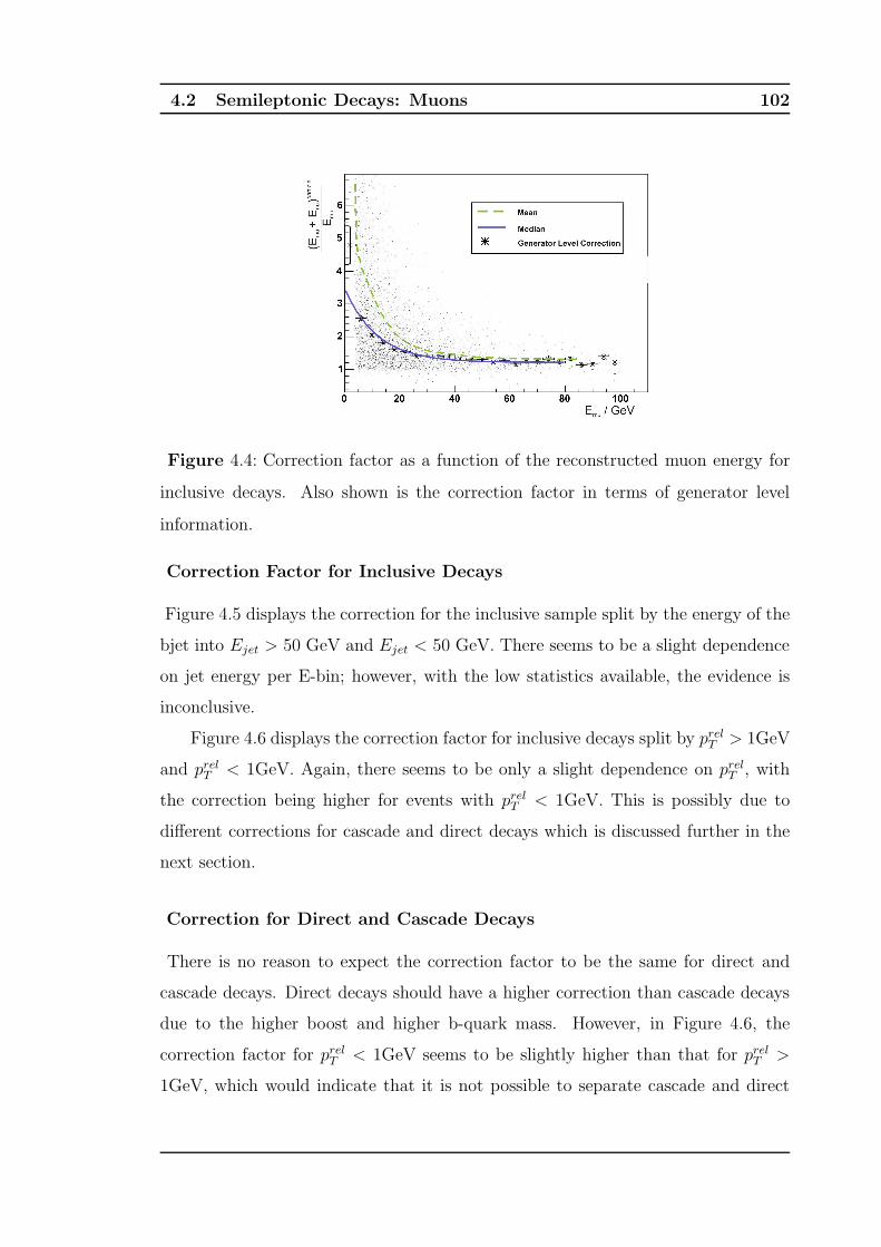
4.2 Semileptonic Decays: Muons 102
Figure 4.4: Correction factor as a function of the reconstructed muon energy for
inclusive decays. Also shown is the correction factor in terms of generator level
information.
Correction Factor for Inclusive Decays
Figure 4.5 displays the correction for the inclusive sample split by the energy of the
bjet into Ejet > 50 GeV and Ejet < 50 GeV. There seems to be a slight dependence
on jet energy per E-bin; however, with the low statistics available, the evidence is
inconclusive.
Figure 4.6 displays the correction factor for inclusive decays split by prelT > 1GeV
and prelT < 1GeV. Again, there seems to be only a slight dependence on prel
T , with
the correction being higher for events with prelT < 1GeV. This is possibly due to
different corrections for cascade and direct decays which is discussed further in the
next section.
Correction for Direct and Cascade Decays
There is no reason to expect the correction factor to be the same for direct and
cascade decays. Direct decays should have a higher correction than cascade decays
due to the higher boost and higher b-quark mass. However, in Figure 4.6, the
correction factor for prelT < 1GeV seems to be slightly higher than that for prel
T >
1GeV, which would indicate that it is not possible to separate cascade and direct
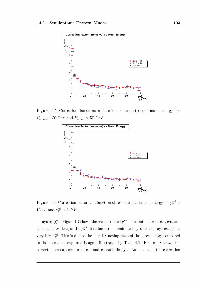
4.2 Semileptonic Decays: Muons 103
(Gev)µE0 20 40 60 80 100
µE
par
ticl
eν
+ E
µE
1
2
3
4
5
6
Correction Factor (inclusive) vs Muon Energy
Jet E > 50Jet E < 50Inclusive
Correction Factor (inclusive) vs Muon Energy
Figure 4.5: Correction factor as a function of reconstructed muon energy for
Eb−jet < 50 GeV and Eb−jet > 50 GeV.
(Gev)µE0 20 40 60 80 100
µE
par
ticl
eν
+ E
µE
1
2
3
4
5
6
Correction Factor (inclusive) vs Muon Energy
pt rel > 1pt rel < 1Inclusive
Correction Factor (inclusive) vs Muon Energy
Figure 4.6: Correction factor as a function of reconstructed muon energy for prelT >
1GeV and prelT < 1GeV
decays by prelT . Figure 4.7 shows the reconstructed prel
T distribution for direct, cascade
and inclusive decays; the prelT distribution is dominated by direct decays except at
very low prelT . This is due to the high branching ratio of the direct decay compared
to the cascade decay and is again illustrated by Table 4.1. Figure 4.8 shows the
correction separately for direct and cascade decays. As expected, the correction
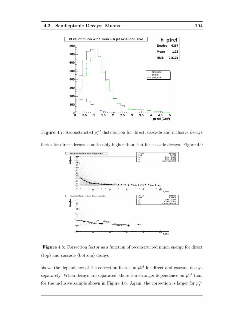
4.2 Semileptonic Decays: Muons 104
_h_ptrelEntries 6387
Mean 1.23
RMS 0.8125
pt rel (GeV)0 0.5 1 1.5 2 2.5 3 3.5 4 4.5 5
0
100
200
300
400
500
600
700
800
_h_ptrelEntries 6387
Mean 1.23
RMS 0.8125
CascadeDirectInclusive
Pt rel of muon w.r.t. muo + b jet axis inclusive
Figure 4.7: Reconstructed prelT distribution for direct, cascade and inclusive decays
factor for direct decays is noticeably higher than that for cascade decays. Figure 4.9
(Gev)µE0 20 40 60 80 100
µE
par
ticl
eν
+ E
µE
1
2
3
4
5
6
7
8
9
/ ndf 2χ 35.56 / 20Prob 0.01732p0 0.0236± 1.216 p1 0.1002± 1.176 p2 0.009007± -0.1005
/ ndf 2χ 35.56 / 20Prob 0.01732p0 0.0236± 1.216 p1 0.1002± 1.176 p2 0.009007± -0.1005
Correction Factor vs Muon Energy (direct)
(Gev)µE0 20 40 60 80 100
µE
par
ticl
eν
+ E
µE
0
1
2
3
4
5
/ ndf 2χ 46.56 / 20Prob 0.000675p0 0.2204± 0.988 p1 0.1629± -0.1005 p2 0.02246± -0.03468
/ ndf 2χ 46.56 / 20Prob 0.000675p0 0.2204± 0.988 p1 0.1629± -0.1005 p2 0.02246± -0.03468
Correction Factor vs Muon Energy (cascade)
Figure 4.8: Correction factor as a function of reconstructed muon energy for direct
(top) and cascade (bottom) decays
shows the dependence of the correction factor on prelT for direct and cascade decays
separately. When decays are separated, there is a stronger dependence on prelT than
for the inclusive sample shown in Figure 4.6. Again, the correction is larger for prelT
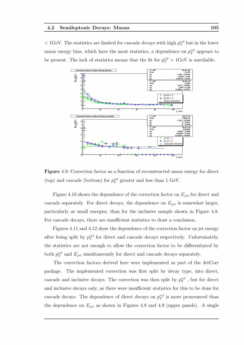
4.2 Semileptonic Decays: Muons 105
< 1GeV. The statistics are limited for cascade decays with high prelT but in the lower
muon energy bins, which have the most statistics, a dependence on prelT appears to
be present. The lack of statistics means that the fit for prelT > 1GeV is unreliable.
(Gev)µE0 20 40 60 80 100
µE
par
ticl
eν
+ E
µE
1
2
3
4
5
6
7
8
9
/ ndf 2χ 35.56 / 20Prob 0.01732p0 0.02357± 1.216 p1 0.1006± 1.176 p2 0.009023± -0.1005
/ ndf 2χ 35.56 / 20Prob 0.01732p0 0.02357± 1.216 p1 0.1006± 1.176 p2 0.009023± -0.1005
/ ndf 2χ 26.91 / 20Prob 0.1379p0 0.03145± 1.194 p1 0.152± 0.8013 p2 0.0132± -0.08778
/ ndf 2χ 26.91 / 20Prob 0.1379p0 0.03145± 1.194 p1 0.152± 0.8013 p2 0.0132± -0.08778
/ ndf 2χ 25.49 / 20Prob 0.1833p0 0.03987± 1.227 p1 0.1106± 1.498 p2 0.01047± -0.09851
/ ndf 2χ 25.49 / 20Prob 0.1833p0 0.03987± 1.227 p1 0.1106± 1.498 p2 0.01047± -0.09851
pt rel > 1pt rel < 1Direct inclusive
Correction Factor vs Muon Energy (direct)
(Gev)µE0 20 40 60 80 100
µE
par
ticl
eν
+ E
µE
0
1
2
3
4
5
/ ndf 2χ 46.56 / 20Prob 0.000675p0 0.2204± 0.988 p1 0.1629± -0.1005 p2 0.02246± -0.03468
/ ndf 2χ 46.56 / 20Prob 0.000675p0 0.2204± 0.988 p1 0.1629± -0.1005 p2 0.02246± -0.03468
/ ndf 2χ 107.8 / 20Prob 4.863e-14p0 0.02338± 1.218 p1 0.4814± -1 p2 0.2438± -2
/ ndf 2χ 107.8 / 20Prob 4.863e-14p0 0.02338± 1.218 p1 0.4814± -1 p2 0.2438± -2
/ ndf 2χ 45.24 / 20Prob 0.001023p0 0.4096± 0.9302 p1 0.1638± 0.09105 p2 0.04518± -0.04196
/ ndf 2χ 45.24 / 20Prob 0.001023p0 0.4096± 0.9302 p1 0.1638± 0.09105 p2 0.04518± -0.04196
pt rel > 1pt rel < 1Cascade inclusive
Correction Factor vs Muon Energy (cascade)
Figure 4.9: Correction factor as a function of reconstructed muon energy for direct
(top) and cascade (bottom) for prelT greater and less than 1 GeV.
Figure 4.10 shows the dependence of the correction factor on Ejet for direct and
cascade separately. For direct decays, the dependence on Ejet is somewhat larger,
particularly at small energies, than for the inclusive sample shown in Figure 4.8.
For cascade decays, there are insufficient statistics to draw a conclusion.
Figures 4.11 and 4.12 show the dependence of the correction factor on jet energy
after being split by prelT for direct and cascade decays respectively. Unfortunately,
the statistics are not enough to allow the correction factor to be differentiated by
both prelT and Ejet simultaneously for direct and cascade decays separately.
The correction factors derived here were implemented as part of the JetCorr
package. The implemented correction was first split by decay type, into direct,
cascade and inclusive decays. The correction was then split by prelT , but for direct
and inclusive decays only, as there were insufficient statistics for this to be done for
cascade decays. The dependence of direct decays on prelT is more pronounced than
the dependence on Ejet as shown in Figures 4.8 and 4.9 (upper panels). A single
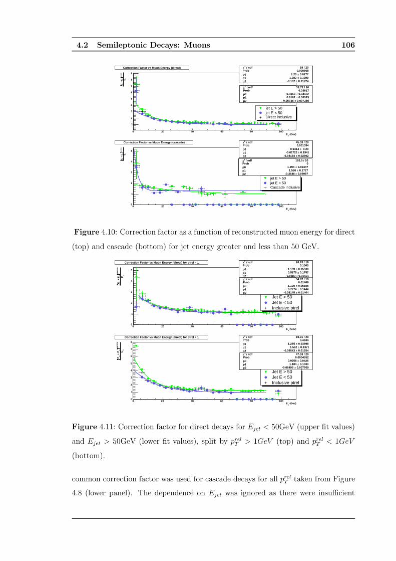
4.2 Semileptonic Decays: Muons 106
(Gev)µE0 20 40 60 80 100
µE
par
ticl
eν
+ E
µE
1
2
3
4
5
6
7
8
9
/ ndf 2χ 35.56 / 20Prob 0.01732p0 0.02357± 1.216 p1 0.1006± 1.176 p2 0.009023± -0.1005
/ ndf 2χ 35.56 / 20Prob 0.01732p0 0.02357± 1.216 p1 0.1006± 1.176 p2 0.009023± -0.1005
/ ndf 2χ 38 / 20Prob 0.008865p0 0.0277± 1.23 p1 0.1399± 1.282 p2 0.01224± -0.102
/ ndf 2χ 38 / 20Prob 0.008865p0 0.0277± 1.23 p1 0.1399± 1.282 p2 0.01224± -0.102
/ ndf 2χ 32.72 / 20Prob 0.03617p0 0.04472± 0.9353 p1 0.08593± 0.8182 p2 0.007285± -0.05736
/ ndf 2χ 32.72 / 20Prob 0.03617p0 0.04472± 0.9353 p1 0.08593± 0.8182 p2 0.007285± -0.05736
jet E > 50jet E < 50Direct inclusive
Correction Factor vs Muon Energy (direct)
(Gev)µE0 20 40 60 80 100
µE
par
ticl
eν
+ E
µE
0
1
2
3
4
5
/ ndf 2χ 46.56 / 20Prob 0.000675p0 0.2204± 0.988 p1 0.1629± -0.1005 p2 0.02246± -0.03468
/ ndf 2χ 46.56 / 20Prob 0.000675p0 0.2204± 0.988 p1 0.1629± -0.1005 p2 0.02246± -0.03468
/ ndf 2χ 45.03 / 20Prob 0.001094p0 0.29± 0.9414 p1 0.1941± -0.01722 p2 0.02302± -0.03134
/ ndf 2χ 45.03 / 20Prob 0.001094p0 0.29± 0.9414 p1 0.1941± -0.01722 p2 0.02302± -0.03134
/ ndf 2χ 193.5 / 20Prob 0p0 0.02447± 1.294 p1 0.1727± 1.526 p2 0.05987± -0.3646
/ ndf 2χ 193.5 / 20Prob 0p0 0.02447± 1.294 p1 0.1727± 1.526 p2 0.05987± -0.3646
jet E > 50jet E < 50Cascade inclusive
Correction Factor vs Muon Energy (cascade)
Figure 4.10: Correction factor as a function of reconstructed muon energy for direct
(top) and cascade (bottom) for jet energy greater and less than 50 GeV.
(Gev)µE0 20 40 60 80 100
µE
par
ticl
eν
+ E
µE
0
1
2
3
4
5
/ ndf 2χ 26.91 / 20Prob 0.1379p0 0.03145± 1.194 p1 0.152± 0.8013 p2 0.0132± -0.08778
/ ndf 2χ 26.91 / 20Prob 0.1379p0 0.03145± 1.194 p1 0.152± 0.8013 p2 0.0132± -0.08778
/ ndf 2χ 26.93 / 19Prob 0.1063p0 0.05538± 1.139 p1 0.1757± 0.5375 p2 0.01421± -0.0589
/ ndf 2χ 26.93 / 19Prob 0.1063p0 0.05538± 1.139 p1 0.1757± 0.5375 p2 0.01421± -0.0589
/ ndf 2χ 34.82 / 19Prob 0.01469p0 0.05155± 1.125 p1 0.1444± 0.7274 p2 0.01404± -0.08145
/ ndf 2χ 34.82 / 19Prob 0.01469p0 0.05155± 1.125 p1 0.1444± 0.7274 p2 0.01404± -0.08145
Jet E > 50 Jet E < 50 Inclusive ptrel
Correction Factor vs Muon Energy (direct) for ptrel > 1
(Gev)µE0 20 40 60 80 100
µE
par
ticl
eν
+ E
µE
0
1
2
3
4
5
6
7
8
/ ndf 2χ 25.49 / 20Prob 0.1833p0 0.03987± 1.227 p1 0.1106± 1.498 p2 0.01047± -0.09851
/ ndf 2χ 25.49 / 20Prob 0.1833p0 0.03987± 1.227 p1 0.1106± 1.498 p2 0.01047± -0.09851
/ ndf 2χ 19.91 / 20Prob 0.4634p0 0.03898± 1.265 p1 0.1371± 1.562 p2 0.01254± -0.09543
/ ndf 2χ 19.91 / 20Prob 0.4634p0 0.03898± 1.265 p1 0.1371± 1.562 p2 0.01254± -0.09543
/ ndf 2χ 47.53 / 20Prob 0.0004952p0 0.0426± 0.9258 p1 0.1033± 1.184 p2 0.007769± -0.06498
/ ndf 2χ 47.53 / 20Prob 0.0004952p0 0.0426± 0.9258 p1 0.1033± 1.184 p2 0.007769± -0.06498
Jet E > 50 Jet E < 50 Inclusive ptrel
Correction Factor vs Muon Energy (direct) for ptrel < 1
Figure 4.11: Correction factor for direct decays for Ejet < 50GeV (upper fit values)
and Ejet > 50GeV (lower fit values), split by prelT > 1GeV (top) and prel
T < 1GeV
(bottom).
common correction factor was used for cascade decays for all prelT taken from Figure
4.8 (lower panel). The dependence on Ejet was ignored as there were insufficient
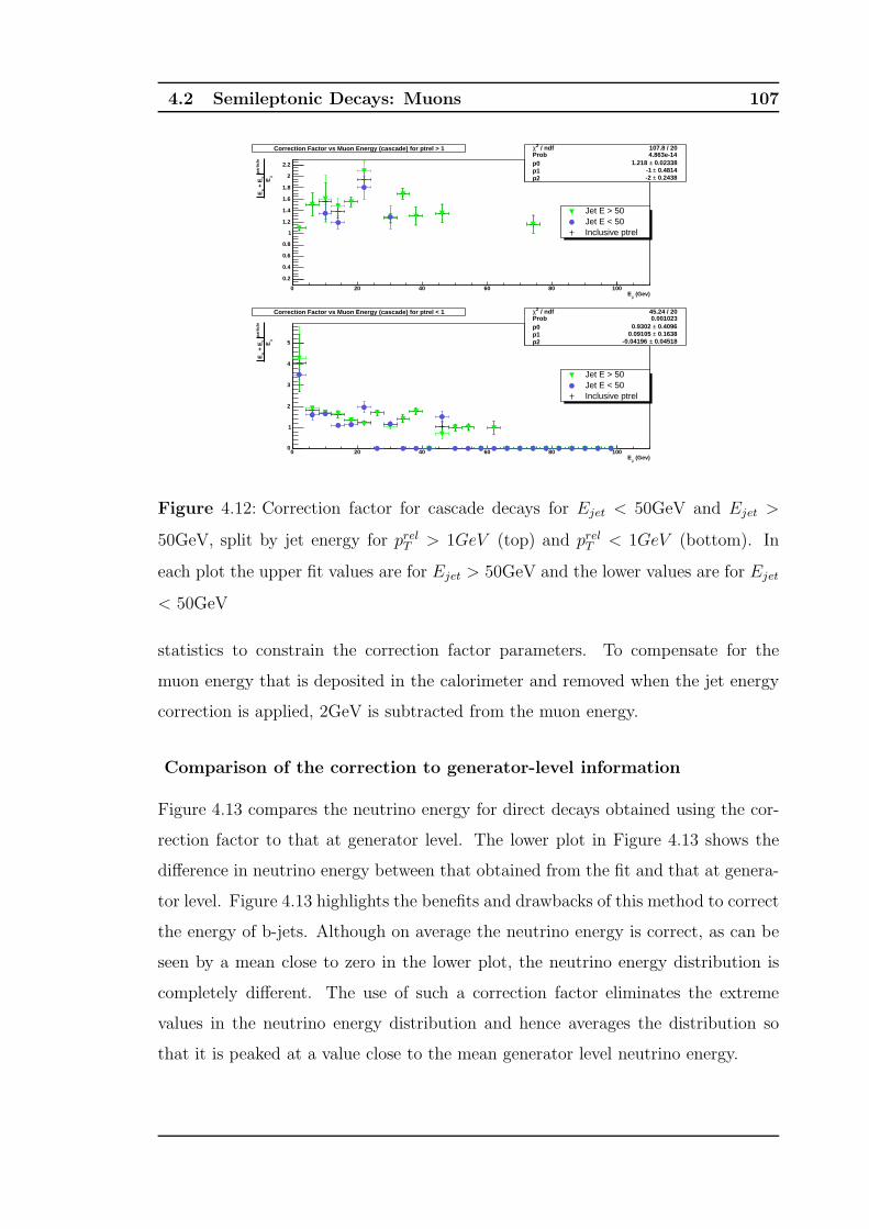
4.2 Semileptonic Decays: Muons 107
(Gev)µE0 20 40 60 80 100
µE
par
ticl
eν
+ E
µE
0.2
0.4
0.6
0.8
1
1.2
1.4
1.6
1.8
2
2.2
/ ndf 2χ 107.8 / 20Prob 4.863e-14p0 0.02338± 1.218 p1 0.4814± -1 p2 0.2438± -2
/ ndf 2χ 107.8 / 20Prob 4.863e-14p0 0.02338± 1.218 p1 0.4814± -1 p2 0.2438± -2
Jet E > 50 Jet E < 50 Inclusive ptrel
Correction Factor vs Muon Energy (cascade) for ptrel > 1
(Gev)µE0 20 40 60 80 100
µE
par
ticl
eν
+ E
µE
0
1
2
3
4
5
/ ndf 2χ 45.24 / 20Prob 0.001023p0 0.4096± 0.9302 p1 0.1638± 0.09105 p2 0.04518± -0.04196
/ ndf 2χ 45.24 / 20Prob 0.001023p0 0.4096± 0.9302 p1 0.1638± 0.09105 p2 0.04518± -0.04196
Jet E > 50 Jet E < 50 Inclusive ptrel
Correction Factor vs Muon Energy (cascade) for ptrel < 1
Figure 4.12: Correction factor for cascade decays for Ejet < 50GeV and Ejet >
50GeV, split by jet energy for prelT > 1GeV (top) and prel
T < 1GeV (bottom). In
each plot the upper fit values are for Ejet > 50GeV and the lower values are for Ejet
< 50GeV
statistics to constrain the correction factor parameters. To compensate for the
muon energy that is deposited in the calorimeter and removed when the jet energy
correction is applied, 2GeV is subtracted from the muon energy.
Comparison of the correction to generator-level information
Figure 4.13 compares the neutrino energy for direct decays obtained using the cor-
rection factor to that at generator level. The lower plot in Figure 4.13 shows the
difference in neutrino energy between that obtained from the fit and that at genera-
tor level. Figure 4.13 highlights the benefits and drawbacks of this method to correct
the energy of b-jets. Although on average the neutrino energy is correct, as can be
seen by a mean close to zero in the lower plot, the neutrino energy distribution is
completely different. The use of such a correction factor eliminates the extreme
values in the neutrino energy distribution and hence averages the distribution so
that it is peaked at a value close to the mean generator level neutrino energy.
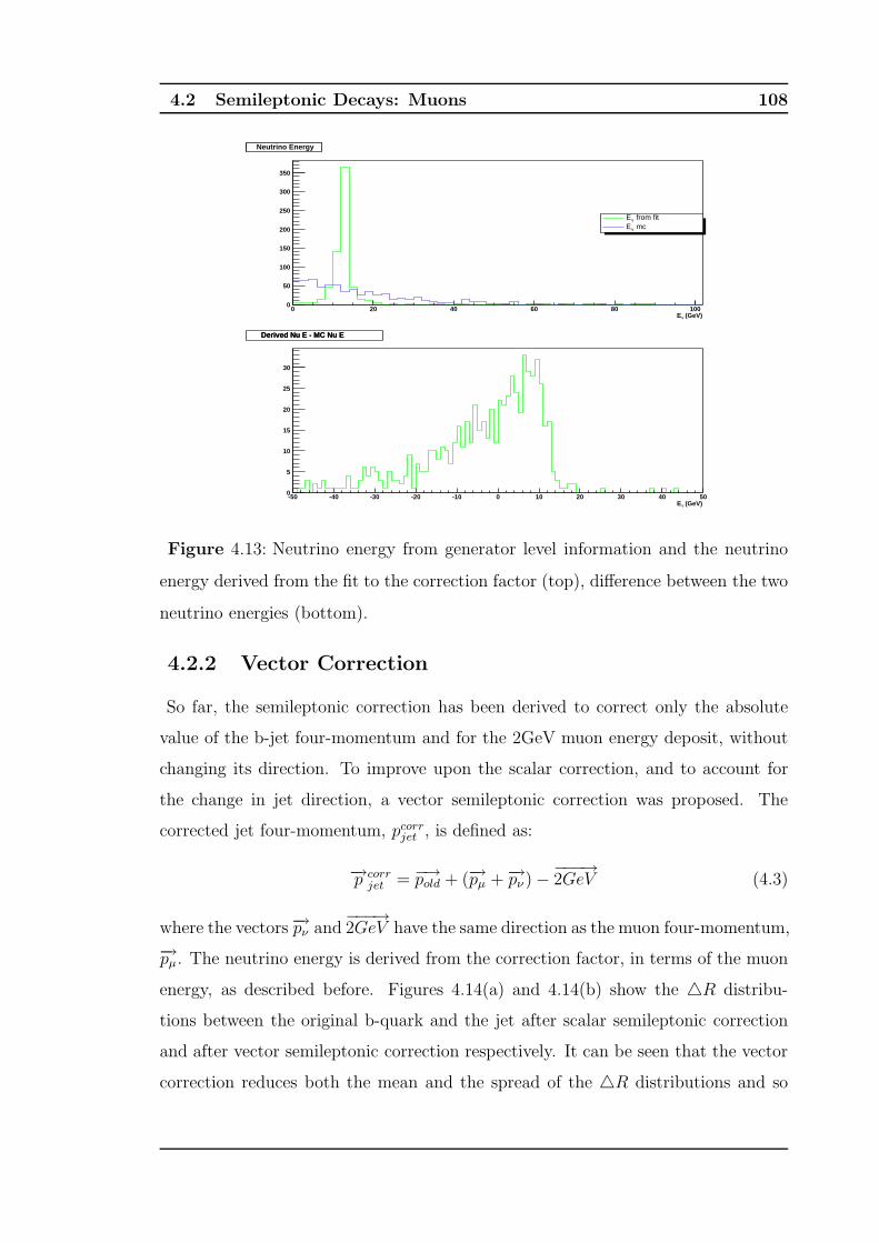
4.2 Semileptonic Decays: Muons 108
(GeV)νE0 20 40 60 80 100
0
50
100
150
200
250
300
350
Neutrino Energy
from fitνE mcνE
Neutrino Energy
(GeV)νE-50 -40 -30 -20 -10 0 10 20 30 40 500
5
10
15
20
25
30
Derived Nu E - MC Nu E Derived Nu E - MC Nu E
Figure 4.13: Neutrino energy from generator level information and the neutrino
energy derived from the fit to the correction factor (top), difference between the two
neutrino energies (bottom).
4.2.2 Vector Correction
So far, the semileptonic correction has been derived to correct only the absolute
value of the b-jet four-momentum and for the 2GeV muon energy deposit, without
changing its direction. To improve upon the scalar correction, and to account for
the change in jet direction, a vector semileptonic correction was proposed. The
corrected jet four-momentum, pcorrjet , is defined as:
−→p corrjet = −→pold + (−→pµ + −→pν ) −−−−→
2GeV (4.3)
where the vectors −→pν and−−−→2GeV have the same direction as the muon four-momentum,
−→pµ. The neutrino energy is derived from the correction factor, in terms of the muon
energy, as described before. Figures 4.14(a) and 4.14(b) show the △R distribu-
tions between the original b-quark and the jet after scalar semileptonic correction
and after vector semileptonic correction respectively. It can be seen that the vector
correction reduces both the mean and the spread of the △R distributions and so
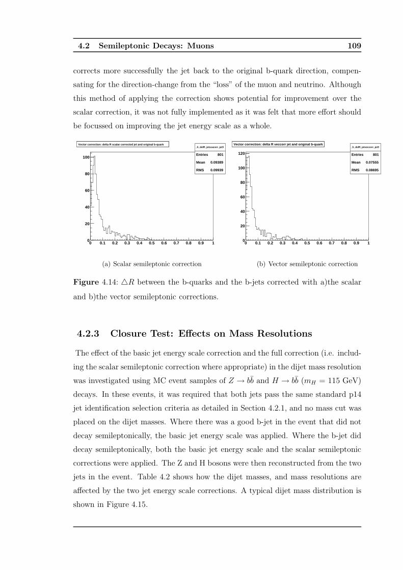
4.2 Semileptonic Decays: Muons 109
corrects more successfully the jet back to the original b-quark direction, compen-
sating for the direction-change from the “loss” of the muon and neutrino. Although
this method of applying the correction shows potential for improvement over the
scalar correction, it was not fully implemented as it was felt that more effort should
be focussed on improving the jet energy scale as a whole.
0 0.1 0.2 0.3 0.4 0.5 0.6 0.7 0.8 0.9 10
20
40
60
80
100
Vector correction: delta R scalar corrected jet and original b-quark_h_delR_jetscacorr_jet3
Entries 801
Mean 0.09389
RMS 0.09939
Vector correction: delta R scalar corrected jet and original b-quark
(a) Scalar semileptonic correction
0 0.1 0.2 0.3 0.4 0.5 0.6 0.7 0.8 0.9 10
20
40
60
80
100
120
Vector correction: delta R veccorr jet and original b-quark_h_delR_jetveccorr_jet3
Entries 801
Mean 0.07555
RMS 0.08695
Vector correction: delta R veccorr jet and original b-quark
(b) Vector semileptonic correction
Figure 4.14: △R between the b-quarks and the b-jets corrected with a)the scalar
and b)the vector semileptonic corrections.
4.2.3 Closure Test: Effects on Mass Resolutions
The effect of the basic jet energy scale correction and the full correction (i.e. includ-
ing the scalar semileptonic correction where appropriate) in the dijet mass resolution
was investigated using MC event samples of Z → bb and H → bb (mH = 115 GeV)
decays. In these events, it was required that both jets pass the same standard p14
jet identification selection criteria as detailed in Section 4.2.1, and no mass cut was
placed on the dijet masses. Where there was a good b-jet in the event that did not
decay semileptonically, the basic jet energy scale was applied. Where the b-jet did
decay semileptonically, both the basic jet energy scale and the scalar semileptonic
corrections were applied. The Z and H bosons were then reconstructed from the two
jets in the event. Table 4.2 shows how the dijet masses, and mass resolutions are
affected by the two jet energy scale corrections. A typical dijet mass distribution is
shown in Figure 4.15.
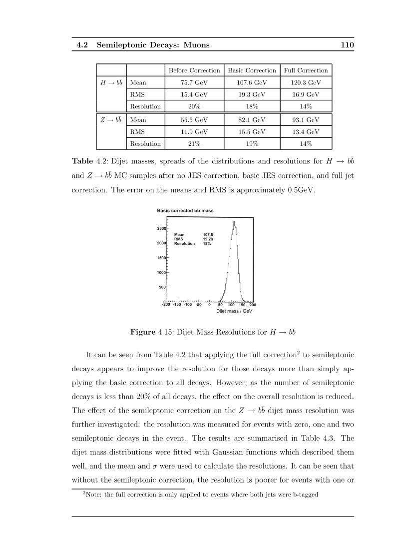
4.2 Semileptonic Decays: Muons 110
Before Correction Basic Correction Full Correction
H → bb Mean 75.7 GeV 107.6 GeV 120.3 GeV
RMS 15.4 GeV 19.3 GeV 16.9 GeV
Resolution 20% 18% 14%
Z → bb Mean 55.5 GeV 82.1 GeV 93.1 GeV
RMS 11.9 GeV 15.5 GeV 13.4 GeV
Resolution 21% 19% 14%
Table 4.2: Dijet masses, spreads of the distributions and resolutions for H → bb
and Z → bb MC samples after no JES correction, basic JES correction, and full jet
correction. The error on the means and RMS is approximately 0.5GeV.
Basic corrected bb massUncorrected bb mass
Fully corrected bb mass
Dijet mass / GeV
Dijet mass / GeV Dijet mass / GeV
Mean 75.68RMS 15.42Resolution 20%
Mean 120.3RMS 16.92Resolution 14%
Mean 107.6RMS 19.28Resolution 18%
Figure 4.15: Dijet Mass Resolutions for H → bb
It can be seen from Table 4.2 that applying the full correction2 to semileptonic
decays appears to improve the resolution for those decays more than simply ap-
plying the basic correction to all decays. However, as the number of semileptonic
decays is less than 20% of all decays, the effect on the overall resolution is reduced.
The effect of the semileptonic correction on the Z → bb dijet mass resolution was
further investigated: the resolution was measured for events with zero, one and two
semileptonic decays in the event. The results are summarised in Table 4.3. The
dijet mass distributions were fitted with Gaussian functions which described them
well, and the mean and σ were used to calculate the resolutions. It can be seen that
without the semileptonic correction, the resolution is poorer for events with one or
2Note: the full correction is only applied to events where both jets were b-tagged
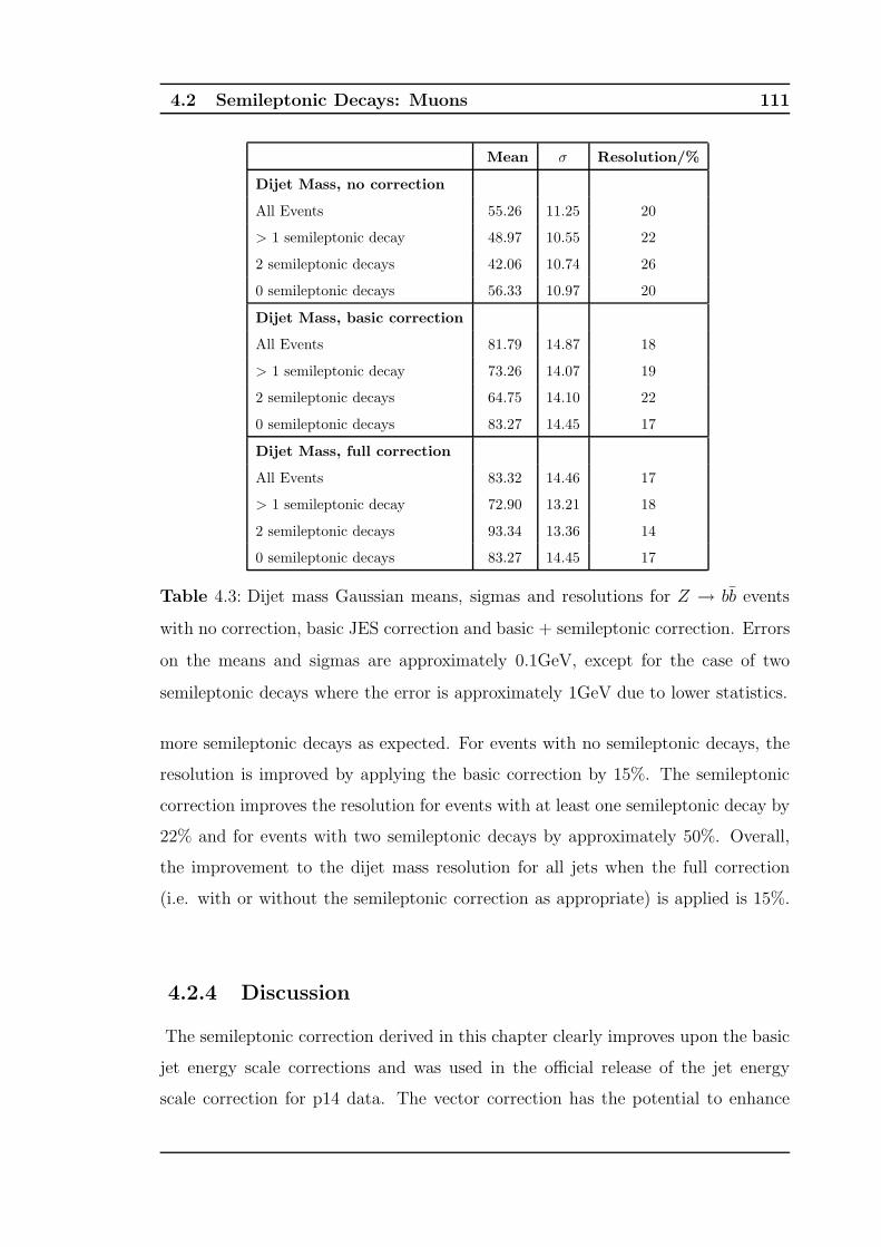
4.2 Semileptonic Decays: Muons 111
Mean σ Resolution/%
Dijet Mass, no correction
All Events 55.26 11.25 20
> 1 semileptonic decay 48.97 10.55 22
2 semileptonic decays 42.06 10.74 26
0 semileptonic decays 56.33 10.97 20
Dijet Mass, basic correction
All Events 81.79 14.87 18
> 1 semileptonic decay 73.26 14.07 19
2 semileptonic decays 64.75 14.10 22
0 semileptonic decays 83.27 14.45 17
Dijet Mass, full correction
All Events 83.32 14.46 17
> 1 semileptonic decay 72.90 13.21 18
2 semileptonic decays 93.34 13.36 14
0 semileptonic decays 83.27 14.45 17
Table 4.3: Dijet mass Gaussian means, sigmas and resolutions for Z → bb events
with no correction, basic JES correction and basic + semileptonic correction. Errors
on the means and sigmas are approximately 0.1GeV, except for the case of two
semileptonic decays where the error is approximately 1GeV due to lower statistics.
more semileptonic decays as expected. For events with no semileptonic decays, the
resolution is improved by applying the basic correction by 15%. The semileptonic
correction improves the resolution for events with at least one semileptonic decay by
22% and for events with two semileptonic decays by approximately 50%. Overall,
the improvement to the dijet mass resolution for all jets when the full correction
(i.e. with or without the semileptonic correction as appropriate) is applied is 15%.
4.2.4 Discussion
The semileptonic correction derived in this chapter clearly improves upon the basic
jet energy scale corrections and was used in the official release of the jet energy
scale correction for p14 data. The vector correction has the potential to enhance

4.3 Energy Flow: Electromagnetic Calorimeter Calibration 112
this semileptonic correction. It remains to consider how this vector correction will
be implemented in both MC and data. The muon momentum in MC is better than
that in data, and so the MC muon momentum should be smeared to match the
MC resolution to that in data. At the time this work was carried out, a muon
MC smearing had not been calculated but was planned and it would be interesting
to see how this affects the semileptonic correction. Furthermore, before the vector
correction could be used, the size of the muon calorimeter MIP energy deposit, set
at 2GeV should be investigated.
4.3 Energy Flow: Electromagnetic Calorimeter
Calibration
A first, illustrative, version of an eflow algorithm was coded in the DØ environment
in 2002 [77]. It is based on the ALEPH package [80]. Preliminary studies, based
on Monte Carlo, have shown jet resolution improvements of about 20% for low and
intermediate energy jets. The next step was to update the basic algorithm and test
it on data, a process that was started in December 2003.
Eflow Particles There are three types of eflow particles produced based on track-
calorimeter associations: charged particles, photons and neutral hadrons. Energy
flow should include information from all the subdetectors, but at DØ , mostly tracker
and calorimeter information is used, with some information from the muon system.
Charged particles are made of one track associated with a calorimeter cluster of
energy, whereas a photon or a neutral hadron is an electromagnetic or hadronic
cluster with no associated track. The energy clusters are calorimeter cells with
energy deposits that have been clustered using a nearest neighbour clustering algo-
rithm, the cellNN algorithm [81], thus a calorimeter cellNN calibration is needed.
Reconstructed tracks are extrapolated through the calorimeter along a straight line
and all clusters crossing the track are matched if their energy is <1% of the track
momentum. 3
3This cut is to strike a balance between matching efficiency and fake associations.
4.3 Energy Flow: Electromagnetic Calorimeter Calibration 113
4.3.1 Towards a Working Algorithm
Eflow is more complicated than a simple calorimeter energy measurement so several
things must be considered. To implement a working eflow algorithm, several calibra-
tions and scales need to be calculated and integrated: a calorimeter cell-level scale
for hadronic and electromagnetic particles scale, accurate cell-level calibrations for
the calorimeter itself, and a tracking scale with understanding of the systematics at
low energy. As stated earlier, effort was redirected back to eflow in December 2003
and one of the necessary steps was to derive a track-EM cell intercalibration In this
section, an electromagnetic scale for calorimeter cell clusters is derived using low
momentum (< 25GeV) MC and data J/Ψ → e+e− event samples. The electromag-
netic scale is calculated using clusters of calorimeter cells that are matched to within
0.2 in η and φ (R<0.2)of a track that has been identified as coming from an electron.
The momentum of the track is taken to give the ‘correct’ energy for the cluster and
a function is derived to map the cluster energy back to the track momentum. The
EM scale is examined for the whole detector as a function of cluster energy and
cluster detector η. Events are chosen to have at least two electrons, matched to
clusters, that reconstruct to give an invariant mass within the J/Ψ resonance peak.
Tracks from Electrons The electrons whose tracks are used in the calculation
of the EM scale are not standard DØ electrons as described in Section 2.2.8, but
are identified using the road algorithm [82], [83]. The standard way of identifying
electrons at DØ relies on the characteristic transverse and longitudinal shapes of
EM showers [84]. This method is efficient for high-energy, isolated electrons, but
it is not efficient for electrons in jets and so the ‘road’ method is used primarily to
identify such electrons. It is based on the extrapolation of charged tracks in the
tracker into the calorimeter; for a given track, only the energy contained in a tube
of R=0.2 (‘road’) along the track extrapolation into the calorimeter is used.
4.3.2 Event Samples and Selection Criteria
A sample of 6560 data events containing at least two EM objects was used as
it was the largest suitable dataset available at the time. It was reprocessed with
4.3 Energy Flow: Electromagnetic Calorimeter Calibration 114
version p14.06.00 [73] of the reconstruction code. The data were skimmed using the
low-energy electron triggers E7A 2RL3 RT3 RL5 and E7B 2RL3 RT3 RL5. Table
4.4 lists the L1, L2 and L3 trigger requirements for these triggers. For comparison
with MC, an event sample containing 13200 J/Ψ → e+e− events, processed using
p14.03.00 and generated using Pythia, was used. The MC was generated for the
central region of the calorimeter only.
Trigger Name E7A 2RL3 RT3 RL5 E7B 2RL3 RT3 RL5
L1 requirements
• Two calorimeter EM objects with ET >3GeV.
• One of the objects must have ET >6GeV.
• Two tracks with pT >3 GeV
• One of these tracks must have pT >5GeV.
L2 requirements
• Two EM objects with ET >3GeV within |η| <1.6.
• One of those objects must have ET > 6GeV
L3 requirements
• Two road electrons with loose cuts and track pT >3GeV.
• One of the electrons also must satisfy tight cuts.
• One of the electrons must have track pT >5 GeV
Table 4.4: Details of the L1, L2 and L3 trigger requirements for the
E7A 2RL3 RT3 RL5 and E7B 2RL3 RT3 RL5
Electron Track Selection
It is required that there are at least two road electrons in the event which pass the
following criteria:
• Isolation ≤ 0.9
• HMx8 ≤ 75
4.3 Energy Flow: Electromagnetic Calorimeter Calibration 115
• Be within the fiducial region of the calorimeter
• Reconstruct to give an invariant mass of between 2.096GeV and 4.096GeV.
(J/Ψ mass ±1GeV)
• Be within |η| <1.25
All road electrons have track matches by definition, and so this was not a se-
lection criterion. The standard isolation cut is to require that Isolation ≤ 0.15.
However, electrons from J/Ψ are likely to not be particularly isolated so this was
loosened to allow more events to pass the cuts. The electrons were also required
to pass the ‘tight’ road electron criteria [85]. Table 4.5 outlines the criteria for
loose, medium and tight road electrons. The kinematic distributions for the elec-
trons/tracks were as expected.
Selection Criteria Loose Road Electron Tight Road Electron
fEM > 0.6 > 0.9
ET > 0 > 0
E/p 0.4 < Ep < 1.3 0.6 < E
p < 1.05
Associated track pT > 3GeV > 3GeV
Table 4.5: Criteria for loose and tight road electrons
CellNN Cluster Selection and Track Matching
CellNN clusters were required to have pT > 3GeV and to be matched to an electron
track within R=0.2 corresponding to the size of a typical EM shower. In the MC
sample, it was found that the two highest energy clusters belong to the e+e−pair from
the J/Ψ when matching was possible. So the clusters were ordered in descending
energy before matching to electron tracks that lie within R<0.2. It was a requirement
that tracks could only be matched to one cluster, but the clusters could be matched
to more than one electron. When this was the case, the closest match in η and φ
was taken. Figure 4.16 shows a scatter plot of Ecluster/ptrack against △R between
the cluster and the matched track for data (left) and MC (right). It can be seen
that tracks and clusters match closely, and that the matching requirement is quite
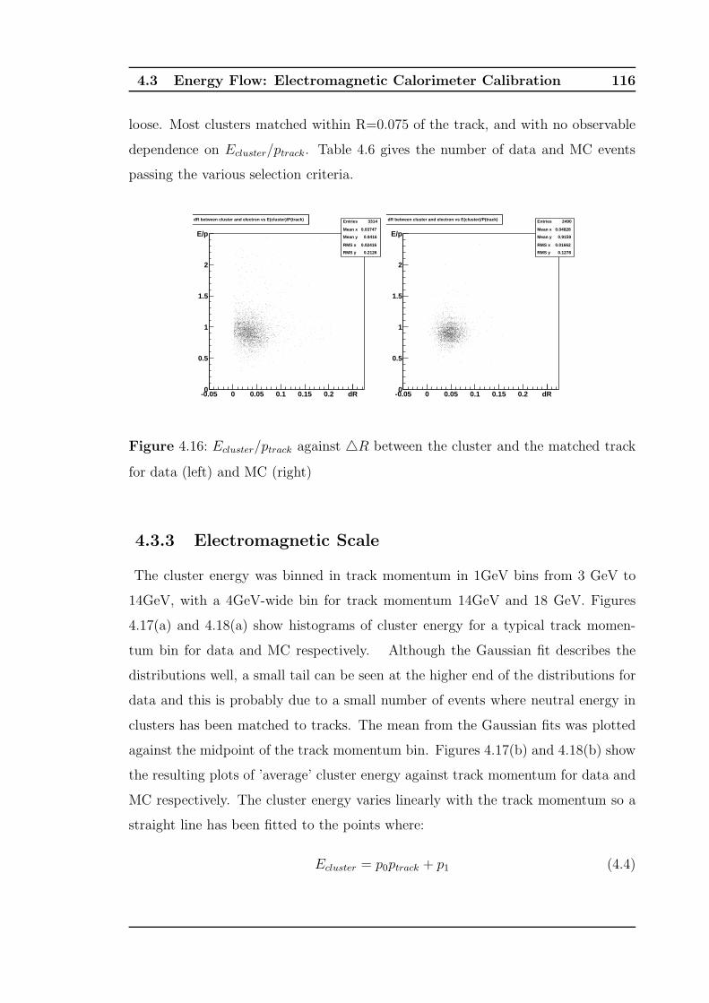
4.3 Energy Flow: Electromagnetic Calorimeter Calibration 116
loose. Most clusters matched within R=0.075 of the track, and with no observable
dependence on Ecluster/ptrack. Table 4.6 gives the number of data and MC events
passing the various selection criteria.
-0.05 0 0.05 0.1 0.15 0.2 dR0
0.5
1
1.5
2
E/p
dR between cluster and electron vs E(cluster)/P(track) Entries 3314
Mean x 0.03747
Mean y 0.9416
RMS x 0.02416
RMS y 0.2126
dR between cluster and electron vs E(cluster)/P(track)
-0.05 0 0.05 0.1 0.15 0.2 dR0
0.5
1
1.5
2
E/p
dR between cluster and electron vs E(cluster)/P(track) Entries 2490
Mean x 0.04828
Mean y 0.9159
RMS x 0.01662
RMS y 0.1278
dR between cluster and electron vs E(cluster)/P(track)
Figure 4.16: Ecluster/ptrack against △R between the cluster and the matched track
for data (left) and MC (right)
4.3.3 Electromagnetic Scale
The cluster energy was binned in track momentum in 1GeV bins from 3 GeV to
14GeV, with a 4GeV-wide bin for track momentum 14GeV and 18 GeV. Figures
4.17(a) and 4.18(a) show histograms of cluster energy for a typical track momen-
tum bin for data and MC respectively. Although the Gaussian fit describes the
distributions well, a small tail can be seen at the higher end of the distributions for
data and this is probably due to a small number of events where neutral energy in
clusters has been matched to tracks. The mean from the Gaussian fits was plotted
against the midpoint of the track momentum bin. Figures 4.17(b) and 4.18(b) show
the resulting plots of ’average’ cluster energy against track momentum for data and
MC respectively. The cluster energy varies linearly with the track momentum so a
straight line has been fitted to the points where:
Ecluster = p0ptrack + p1 (4.4)
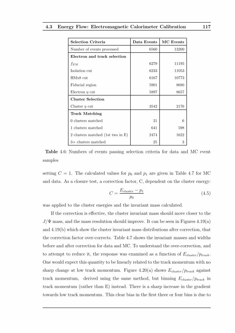
4.3 Energy Flow: Electromagnetic Calorimeter Calibration 117
Selection Criteria Data Events MC Events
Number of events processed 6560 13200
Electron and track selection
fEM 6279 11195
Isolation cut 6233 11053
HMx8 cut 6167 10773
Fiducial region 5901 8680
Electron η cut 5897 8657
Cluster Selection
Cluster η cut 3542 2176
Track Matching
0 clusters matched 21 6
1 clusters matched 641 598
2 clusters matched (1st two in E) 2474 1622
3+ clusters matched 25 3
Table 4.6: Numbers of events passing selection criteria for data and MC event
samples
setting C = 1. The calculated values for p0 and p1 are given in Table 4.7 for MC
and data. As a closure test, a correction factor, C, dependent on the cluster energy:
C =Ecluster − p1
p0(4.5)
was applied to the cluster energies and the invariant mass calculated.
If the correction is effective, the cluster invariant mass should move closer to the
J/Ψ mass, and the mass resolution should improve. It can be seen in Figures 4.19(a)
and 4.19(b) which show the cluster invariant mass distributions after correction, that
the correction factor over-corrects. Table 4.7 shows the invariant masses and widths
before and after correction for data and MC. To understand the over-correction, and
to attempt to reduce it, the response was examined as a function of Ecluster/ptrack.
One would expect this quantity to be linearly related to the track momentum with no
sharp change at low track momentum. Figure 4.20(a) shows Ecluster/ptrack against
track momentum, derived using the same method, but binning Ecluster/ptrack in
track momentum (rather than E) instead. There is a sharp increase in the gradient
towards low track momentum. This clear bias in the first three or four bins is due to
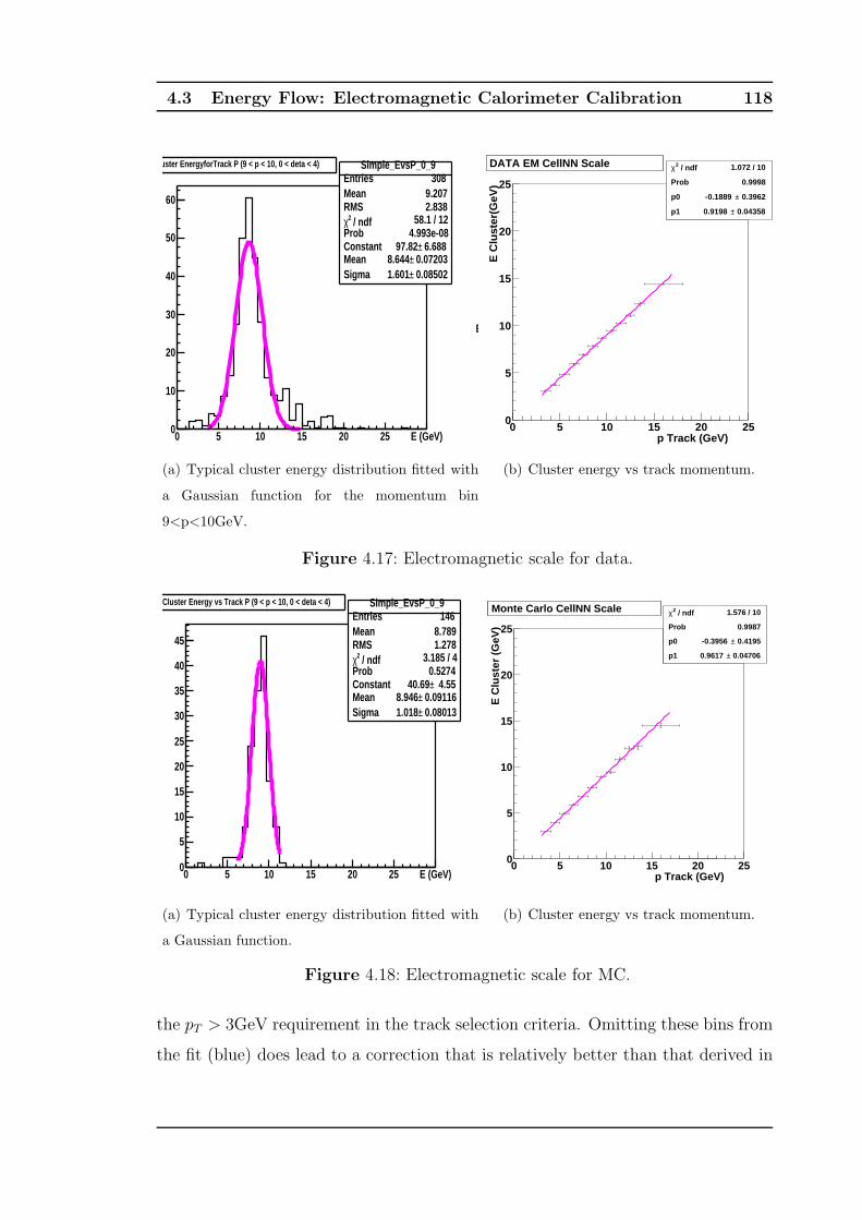
4.3 Energy Flow: Electromagnetic Calorimeter Calibration 118
0 5 10 15 20 25 E (GeV)0
10
20
30
40
50
60
Cluster EnergyforTrack P (9 < p < 10, 0 < deta < 4) Simple_EvsP_0_9Entries 308Mean 9.207RMS 2.838
/ ndf 2χ 58.1 / 12Prob 4.993e-08Constant 6.688± 97.82 Mean 0.07203± 8.644 Sigma 0.08502± 1.601
Cluster EnergyforTrack P (9 < p < 10, 0 < deta < 4)
E (GeV)
(a) Typical cluster energy distribution fitted with
a Gaussian function for the momentum bin
9<p<10GeV.
p Track (GeV)0 5 10 15 20 25
E C
lust
er(G
eV)
0
5
10
15
20
25
DATA CARLO Response Plots / ndf 2χ 1.072 / 10
Prob 0.9998
p0 0.3962± -0.1889
p1 0.04358± 0.9198
/ ndf 2χ 1.072 / 10
Prob 0.9998
p0 0.3962± -0.1889
p1 0.04358± 0.9198
DATA EM CellNN Scale
(b) Cluster energy vs track momentum.
Figure 4.17: Electromagnetic scale for data.
0 5 10 15 20 25 E (GeV)0
5
10
15
20
25
30
35
40
45
Cluster Energy vs Track P (9 < p < 10, 0 < deta < 4) Simple_EvsP_0_9Entries 146Mean 8.789RMS 1.278
/ ndf 2χ 3.185 / 4Prob 0.5274Constant 4.55± 40.69 Mean 0.09116± 8.946 Sigma 0.08013± 1.018
Cluster Energy vs Track P (9 < p < 10, 0 < deta < 4)
(a) Typical cluster energy distribution fitted with
a Gaussian function.
p Track (GeV)0 5 10 15 20 25
E C
lust
er (
GeV
)
0
5
10
15
20
25
Monte Carlo CellNN Scale / ndf 2χ 1.576 / 10
Prob 0.9987
p0 0.4195± -0.3956
p1 0.04706± 0.9617
/ ndf 2χ 1.576 / 10
Prob 0.9987
p0 0.4195± -0.3956
p1 0.04706± 0.9617
Monte Carlo CellNN Scale
(b) Cluster energy vs track momentum.
Figure 4.18: Electromagnetic scale for MC.
the pT > 3GeV requirement in the track selection criteria. Omitting these bins from
the fit (blue) does lead to a correction that is relatively better than that derived in
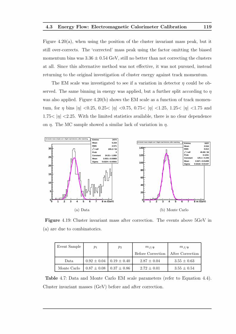
4.3 Energy Flow: Electromagnetic Calorimeter Calibration 119
Figure 4.20(a), when using the position of the cluster invariant mass peak, but it
still over-corrects. The ‘corrected’ mass peak using the factor omitting the biased
momentum bins was 3.36 ± 0.54 GeV, still no better than not correcting the clusters
at all. Since this alternative method was not effective, it was not pursued, instead
returning to the original investigation of cluster energy against track momentum.
The EM scale was investigated to see if a variation in detector η could be ob-
served. The same binning in energy was applied, but a further split according to η
was also applied. Figure 4.20(b) shows the EM scale as a function of track momen-
tum, for η bins |η| <0.25, 0.25< |η| <0.75, 0.75< |η| <1.25, 1.25< |η| <1.75 and
1.75< |η| <2.25. With the limited statistics available, there is no clear dependence
on η. The MC sample showed a similar lack of variation in η.
0 1 2 3 4 5 6 7 8 m (GeV)0
5
10
15
20
25
30
di-cluster mass simple corr: 2tight road electron, after matching Entries 2474
Mean 5.234
RMS 2.571
/ ndf 2χ 205.2 / 53
Prob 0
Constant 1.959± 24.51
Mean 0.03865± 3.553
Sigma 0.03561± 0.6324
di-cluster mass simple corr: 2tight road electron, after matching
(a) Data
0 1 2 3 4 5 6 7 8 m (GeV)
Entries 1622Mean 3.516RMS 0.612
/ ndf 2χ 45.99 / 36Prob 0.1231Constant 4.245± 125.1
Mean 0.01499± 3.547 Sigma 0.01107± 0.5418
0 1 2 3 4 5 6 7 8 m (GeV)0
20
40
60
80
100
120
140
Entries 1622Mean 3.516RMS 0.612
/ ndf 2χ 45.99 / 36Prob 0.1231Constant 4.245± 125.1
Mean 0.01499± 3.547 Sigma 0.01107± 0.5418
di-cluster mass simple corr: 2tight road electron, after matching
(b) Monte Carlo
Figure 4.19: Cluster invariant mass after correction. The events above 5GeV in
(a) are due to combinatorics.
Event Sample p1 p2 mJ/Ψ mJ/Ψ
Before Correction After Correction
Data 0.92 ± 0.04 0.19 ± 0.40 2.87 ± 0.04 3.55 ± 0.63
Monte Carlo 0.87 ± 0.08 0.37 ± 0.86 2.72 ± 0.01 3.55 ± 0.54
Table 4.7: Data and Monte Carlo EM scale parameters (refer to Equation 4.4).
Cluster invariant masses (GeV) before and after correction.
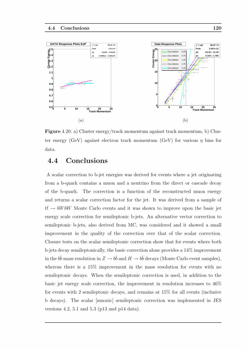
4.4 Conclusions 120
Track Momentum0 5 10 15 20 25
Clu
ster
En
erg
y
0.5
0.6
0.7
0.8
0.9
1
1.1
1.2
1.3
1.4
1.5
DATA Response Plots EoP / ndf 2χ 85.44 / 10
Prob 4.27e-14
p0 0.01032± 0.8193
p1 0.001137± 0.008511
/ ndf 2χ 85.44 / 10
Prob 4.27e-14
p0 0.01032± 0.8193
p1 0.001137± 0.008511
DATA Response Plots EoP
(a)
Track Momentum0 5 10 15 20 25
Clu
ster
En
erg
y
0
5
10
15
20
25
Data Response Plots / ndf 2χ 12.25 / 11
Prob 0.3455
p0 0.4951± -1.911
p1 0.05383± 1.171
/ ndf 2χ 12.25 / 11
Prob 0.3455
p0 0.4951± -1.911
p1 0.05383± 1.171
/ ndf 2χ 18.45 / 11
Prob 0.07177
p0 0.5613± -2.737
p1 0.06102± 1.32
/ ndf 2χ 18.45 / 11
Prob 0.07177
p0 0.5613± -2.737
p1 0.06102± 1.32
/ ndf 2χ 5.424 / 11
Prob 0.9089
p0 0.6243± -4.718
p1 0.06709± 1.38
/ ndf 2χ 5.424 / 11
Prob 0.9089
p0 0.6243± -4.718
p1 0.06709± 1.38
/ ndf 2χ 15.43 / 8
Prob 0.05123
p0 1.501± -3.555
p1 0.1393± 1.467
/ ndf 2χ 15.43 / 8
Prob 0.05123
p0 1.501± -3.555
p1 0.1393± 1.467
/ ndf 2χ 86.87 / 8
Prob 2.007e-15
p0 21.43± -52.35
p1 1.765± 5.316
/ ndf 2χ 86.87 / 8
Prob 2.007e-15
p0 21.43± -52.35
p1 1.765± 5.316
Clus deteta= 0.25
Clus deteta= 0.75
Clus deteta= 1.25
Clus deteta= 1.75
Clus deteta= 2.25
Data Response Plots
(b)
Figure 4.20: a) Cluster energy/track momentum against track momentum, b) Clus-
ter energy (GeV) against electron track momentum (GeV) for various η bins for
data.
4.4 Conclusions
A scalar correction to b-jet energies was derived for events where a jet originating
from a b-quark contains a muon and a neutrino from the direct or cascade decay
of the b-quark. The correction is a function of the reconstructed muon energy
and returns a scalar correction factor for the jet. It was derived from a sample of
tt → bWbW Monte Carlo events and it was shown to improve upon the basic jet
energy scale correction for semileptonic b-jets. An alternative vector correction to
semileptonic b-jets, also derived from MC, was considered and it showed a small
improvement in the quality of the correction over that of the scalar correction.
Closure tests on the scalar semileptonic correction show that for events where both
b-jets decay semileptonically, the basic correction alone provides a 14% improvement
in the bbmass resolution in Z → bb andH → bb decays (Monte Carlo event samples),
whereas there is a 15% improvement in the mass resolution for events with no
semileptonic decays. When the semileptonic correction is used, in addition to the
basic jet energy scale correction, the improvement in resolution increases to 46%
for events with 2 semileptonic decays, and remains at 15% for all events (inclusive
b decays). The scalar [muonic] semileptonic correction was implemented in JES
versions 4.2, 5.1 and 5.3 (p13 and p14 data).
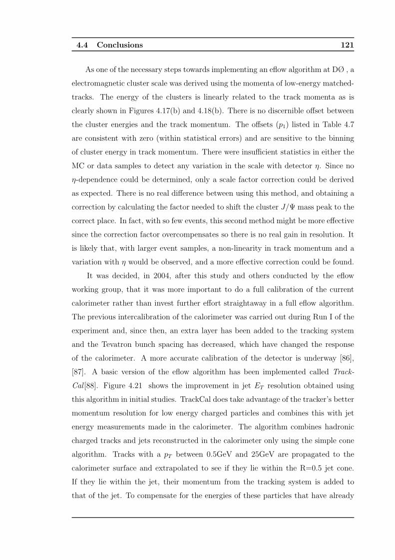
4.4 Conclusions 121
As one of the necessary steps towards implementing an eflow algorithm at DØ , a
electromagnetic cluster scale was derived using the momenta of low-energy matched-
tracks. The energy of the clusters is linearly related to the track momenta as is
clearly shown in Figures 4.17(b) and 4.18(b). There is no discernible offset between
the cluster energies and the track momentum. The offsets (p1) listed in Table 4.7
are consistent with zero (within statistical errors) and are sensitive to the binning
of cluster energy in track momentum. There were insufficient statistics in either the
MC or data samples to detect any variation in the scale with detector η. Since no
η-dependence could be determined, only a scale factor correction could be derived
as expected. There is no real difference between using this method, and obtaining a
correction by calculating the factor needed to shift the cluster J/Ψ mass peak to the
correct place. In fact, with so few events, this second method might be more effective
since the correction factor overcompensates so there is no real gain in resolution. It
is likely that, with larger event samples, a non-linearity in track momentum and a
variation with η would be observed, and a more effective correction could be found.
It was decided, in 2004, after this study and others conducted by the eflow
working group, that it was more important to do a full calibration of the current
calorimeter rather than invest further effort straightaway in a full eflow algorithm.
The previous intercalibration of the calorimeter was carried out during Run I of the
experiment and, since then, an extra layer has been added to the tracking system
and the Tevatron bunch spacing has decreased, which have changed the response
of the calorimeter. A more accurate calibration of the detector is underway [86],
[87]. A basic version of the eflow algorithm has been implemented called Track-
Cal [88]. Figure 4.21 shows the improvement in jet ET resolution obtained using
this algorithm in initial studies. TrackCal does take advantage of the tracker’s better
momentum resolution for low energy charged particles and combines this with jet
energy measurements made in the calorimeter. The algorithm combines hadronic
charged tracks and jets reconstructed in the calorimeter only using the simple cone
algorithm. Tracks with a pT between 0.5GeV and 25GeV are propagated to the
calorimeter surface and extrapolated to see if they lie within the R=0.5 jet cone.
If they lie within the jet, their momentum from the tracking system is added to
that of the jet. To compensate for the energies of these particles that have already
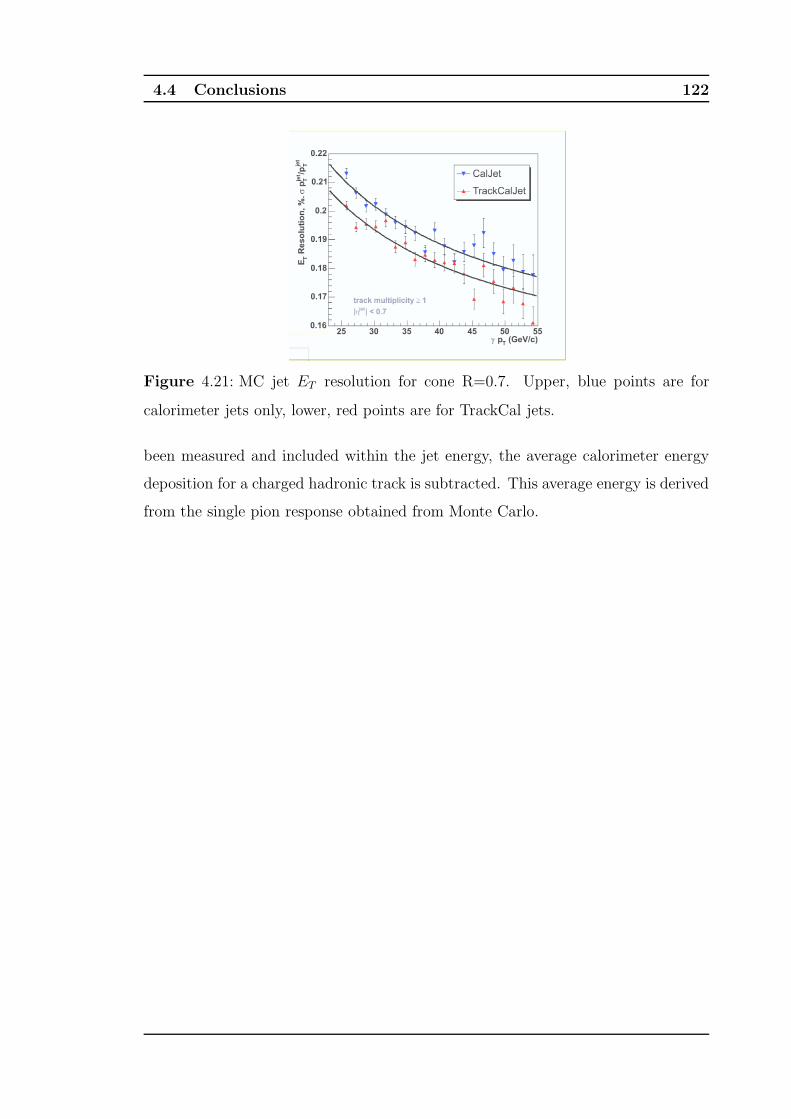
4.4 Conclusions 122
Figure 4.21: MC jet ET resolution for cone R=0.7. Upper, blue points are for
calorimeter jets only, lower, red points are for TrackCal jets.
been measured and included within the jet energy, the average calorimeter energy
deposition for a charged hadronic track is subtracted. This average energy is derived
from the single pion response obtained from Monte Carlo.

5 Search for the Standard Model Higgs Boson 123
Chapter 5
Search for the Standard Model
Higgs Boson
5.1 Introduction
The search for the Higgs boson, one of the truly basic particles and the least ex-
perimentally verified part of the Standard Model, dominates the Run II physics
programme at DØ , and this analysis focuses on a search for the Standard Model
Higgs boson. If the Higgs boson exists, the Tevatron is well-placed to produce evi-
dence of it, and perhaps even discover it as it operates at a centre of mass energy
that means it has sensitivity in the right mass range (. 200GeV) [6]. The phe-
nomenology of the Higgs boson and the global search strategies at the Tevatron are
well known and have been studied in detail in [89][7].
Direct searches at LEP2 set a 95% C.L. lower limit on the mass of the standard
model Higgs boson, mH , of 114.4GeV [26]. Indirect constraints favour a light Higgs
boson [3].
At the Tevatron, there are four important Higgs boson production mechanisms,
and Figure 5.1 shows the production cross-sections as a function of the Higgs mass,
from [7]. The most significant obstacle for Higgs searches is filtering out the large
QCD background of pp collisions and this, in turn, affects which Higgs production
mechanisms and decay channels may be most easily searched for.
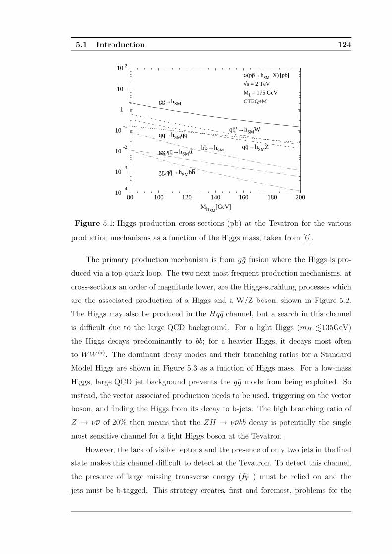
5.1 Introduction 124
σ(pp_→hSM+X) [pb]
√s = 2 TeV
Mt = 175 GeV
CTEQ4Mgg→hSM
qq→hSMqqqq
_’→hSMW
qq_→hSMZ
gg,qq_→hSMtt
_
gg,qq_→hSMbb
_
bb_→hSM
Mh [GeV]SM
10-4
10-3
10-2
10-1
1
10
10 2
80 100 120 140 160 180 200
Figure 5.1: Higgs production cross-sections (pb) at the Tevatron for the various
production mechanisms as a function of the Higgs mass, taken from [6].
The primary production mechanism is from gg fusion where the Higgs is pro-
duced via a top quark loop. The two next most frequent production mechanisms, at
cross-sections an order of magnitude lower, are the Higgs-strahlung processes which
are the associated production of a Higgs and a W/Z boson, shown in Figure 5.2.
The Higgs may also be produced in the Hqq channel, but a search in this channel
is difficult due to the large QCD background. For a light Higgs (mH .135GeV)
the Higgs decays predominantly to bb; for a heavier Higgs, it decays most often
to WW (∗). The dominant decay modes and their branching ratios for a Standard
Model Higgs are shown in Figure 5.3 as a function of Higgs mass. For a low-mass
Higgs, large QCD jet background prevents the gg mode from being exploited. So
instead, the vector associated production needs to be used, triggering on the vector
boson, and finding the Higgs from its decay to b-jets. The high branching ratio of
Z → νν of 20% then means that the ZH → ννbb decay is potentially the single
most sensitive channel for a light Higgs boson at the Tevatron.
However, the lack of visible leptons and the presence of only two jets in the final
state makes this channel difficult to detect at the Tevatron. To detect this channel,
the presence of large missing transverse energy (E/T ) must be relied on and the
jets must be b-tagged. This strategy creates, first and foremost, problems for the
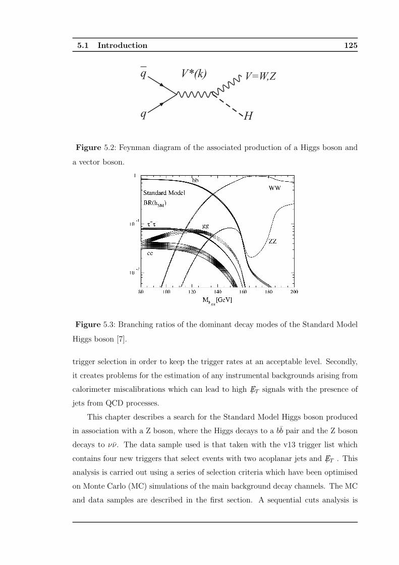
5.1 Introduction 125
q
q
H
V*(k) V=W,Z
Figure 5.2: Feynman diagram of the associated production of a Higgs boson and
a vector boson.
Figure 5.3: Branching ratios of the dominant decay modes of the Standard Model
Higgs boson [7].
trigger selection in order to keep the trigger rates at an acceptable level. Secondly,
it creates problems for the estimation of any instrumental backgrounds arising from
calorimeter miscalibrations which can lead to high E/T signals with the presence of
jets from QCD processes.
This chapter describes a search for the Standard Model Higgs boson produced
in association with a Z boson, where the Higgs decays to a bb pair and the Z boson
decays to νν. The data sample used is that taken with the v13 trigger list which
contains four new triggers that select events with two acoplanar jets and E/T . This
analysis is carried out using a series of selection criteria which have been optimised
on Monte Carlo (MC) simulations of the main background decay channels. The MC
and data samples are described in the first section. A sequential cuts analysis is
5.2 Data and Monte Carlo Event Samples Used 126
carried out and described in Section 5.3. This analysis allows the effects of cutting
on the key signal/background discriminating variables to be observed separately,
and a comparison of MC and data to be made. Advanced techniques to optimise
the MC event selection criteria and the b-tagging have been used to improve the
sensitivity, and these are evaluated in Section 5.4. The systematic uncertainties and
results for the limit on the ZH cross-section are given in Sections 5.5 and . This
analysis is based on the preliminary DØ analysis presented at Moriond ’05 [90] using
the data taken with the v12 trigger list (without acoplanar triggers).
5.2 Data and Monte Carlo Event Samples Used
5.2.1 Data Set
The analysed data were taken from the 28th of June 2004 (run 194567) to the 23rd
of August 2004 (run 196584), with a total luminosity of 55.25pb−1 . The data were
taken with the v13 version of the trigger list which contained four new triggers that
select events with acoplanar jets and missing transverse energy. The data taken
were skimmed for events passing one or more of the 10 triggers listed in Figure 5.4.
Of these 10 triggers, only events firing four of them are of interest to this analysis
and these are described later in this section. The data were reconstructed with
p14.06.01 [91], passed through the thumbnail correction software p14.fixtmb2.02
[92] and passed through d0correct v8.1 [66]. Bad calorimeter, muon, CFT and SMT
runs from the Run Quality Database were eliminated, removing a total of 193 bad
runs. Furthermore, a total of 37973 bad luminosity blocks were eliminated.
5.2.2 Monte Carlo
The signal and background samples used are listed in Tables 5.2 and 5.3, along
with their cross-sections×branching ratios and their SAM1 request ID numbers. The
Z+jets and the W+jets background samples used in this analysis are generated by
1SAM: Sequential Access Metadata. This is the storage facility for our MC and data, stored
under ID numbers.

5.2 Data and Monte Carlo Event Samples Used 127
ALPGEN [93] with the showering and hadronisation processes modelled by Pythia
[74], with p14 minimum bias events overlain . The cross-sections × branching ratios
for these samples are based on leading order ALPGEN calculations multiplied by a
K-factor2 obtained from MCFM3, [94]. The main backgrounds that are simulated
by the MC include Zjj/Zbb, W+jets/Wbb, WZ, ZZ, and top quark production
with jets or escaping leptons. The instrumental background, which is mainly QCD
multijet events, cannot be effectively modelled in MC due to the large cross-section
and small acceptance, so this background is extracted from data and described in
Section 5.3.3.
5.2.3 Trigger Terms
The four trigger terms of interest for this analysis were the set of ‘acoplanar’ [95]
triggers which were all in the same exposure group4 . The v13 trigger list was de-
signed to run up to luminosities of 1032cm−2s−1. This set of acoplanarity triggers
share the same Level 1 and Level 2 trigger requirements and some Level 3 require-
ments. In addition, these four triggers each have further individual L3 requirements
and these are listed below with the common requirements in Table 5.1.
2K-factor: also called a fudge factor, this is a way to express unknown or difficult-to-express
effects with a correction factor. A K-factor is used in comparing cross-sections calculated up to
leading order (LO), to the same up to next-to-leading order (NLO) (K = σNLO/σLO), or in
comparing observed values of cross-sections to those calculated.3MCFM is a parton-level Monte Carlo program which gives NLO predictions for processes at
hadron colliders4Triggers in a Trigger List sharing a set of scalers are called an Exposure Group

5.2 Data and Monte Carlo Event Samples Used 128
Trigger JT1 ACO MHT ER2 JT1 ACO MHT BDV JT1 ACO MHT HT JT1 ACO MHT LM0
L1 Three calorimeter towers with an ET < 5GeV
L2 E/T from jets > 20GeV
Two jets, with the leading two separated by 0 < φ < 168.75◦
L3 One jet with a ET > 9GeV
The φ angle between the two leading jets < 170◦
The vector sum of the pT of all jets (with a pT > 15GeV and with |η| < 2.5) must
be > 30GeV
Other Requires an extra
road electron.
Requires one jet to
be b-tagged and a
primary vertex with
|z| < 35cm.
Requires that scalar
sum of pT of all jets
(with pT > 15GeV
and with |η| < 2.5)
must be > 50GeV.
Requires a loose
muon to be present
at L3.
Table 5.1: Details of the L1, L2 and L3 trigger requirements for the four acopla-
narity triggers used in this analysis.
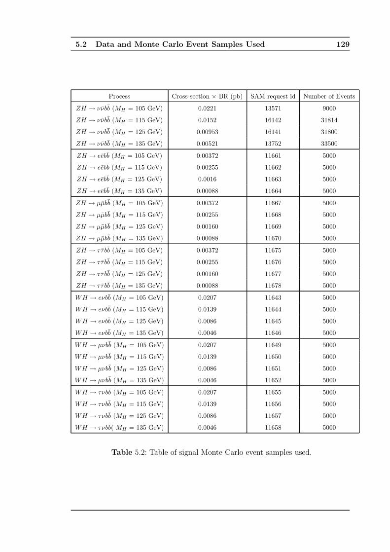
5.2 Data and Monte Carlo Event Samples Used 129
Process Cross-section × BR (pb) SAM request id Number of Events
ZH → ννbb (MH = 105 GeV) 0.0221 13571 9000
ZH → ννbb (MH = 115 GeV) 0.0152 16142 31814
ZH → ννbb (MH = 125 GeV) 0.00953 16141 31800
ZH → ννbb (MH = 135 GeV) 0.00521 13752 33500
ZH → eebb (MH = 105 GeV) 0.00372 11661 5000
ZH → eebb (MH = 115 GeV) 0.00255 11662 5000
ZH → eebb (MH = 125 GeV) 0.0016 11663 5000
ZH → eebb (MH = 135 GeV) 0.00088 11664 5000
ZH → µµbb (MH = 105 GeV) 0.00372 11667 5000
ZH → µµbb (MH = 115 GeV) 0.00255 11668 5000
ZH → µµbb (MH = 125 GeV) 0.00160 11669 5000
ZH → µµbb (MH = 135 GeV) 0.00088 11670 5000
ZH → τ τ bb (MH = 105 GeV) 0.00372 11675 5000
ZH → τ τ bb (MH = 115 GeV) 0.00255 11676 5000
ZH → τ τ bb (MH = 125 GeV) 0.00160 11677 5000
ZH → τ τ bb (MH = 135 GeV) 0.00088 11678 5000
WH → eνbb (MH = 105 GeV) 0.0207 11643 5000
WH → eνbb (MH = 115 GeV) 0.0139 11644 5000
WH → eνbb (MH = 125 GeV) 0.0086 11645 5000
WH → eνbb (MH = 135 GeV) 0.0046 11646 5000
WH → µνbb (MH = 105 GeV) 0.0207 11649 5000
WH → µνbb (MH = 115 GeV) 0.0139 11650 5000
WH → µνbb (MH = 125 GeV) 0.0086 11651 5000
WH → µνbb (MH = 135 GeV) 0.0046 11652 5000
WH → τνbb (MH = 105 GeV) 0.0207 11655 5000
WH → τνbb (MH = 115 GeV) 0.0139 11656 5000
WH → τνbb (MH = 125 GeV) 0.0086 11657 5000
WH → τνbb( MH = 135 GeV) 0.0046 11658 5000
Table 5.2: Table of signal Monte Carlo event samples used.
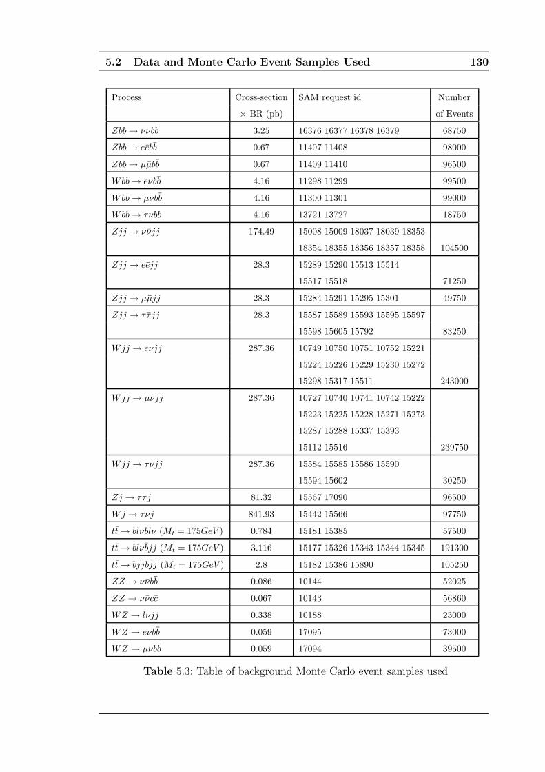
5.2 Data and Monte Carlo Event Samples Used 130
Process Cross-section SAM request id Number
× BR (pb) of Events
Zbb → ννbb 3.25 16376 16377 16378 16379 68750
Zbb → eebb 0.67 11407 11408 98000
Zbb → µµbb 0.67 11409 11410 96500
Wbb → eνbb 4.16 11298 11299 99500
Wbb → µνbb 4.16 11300 11301 99000
Wbb → τνbb 4.16 13721 13727 18750
Zjj → ννjj 174.49 15008 15009 18037 18039 18353
18354 18355 18356 18357 18358 104500
Zjj → eejj 28.3 15289 15290 15513 15514
15517 15518 71250
Zjj → µµjj 28.3 15284 15291 15295 15301 49750
Zjj → τ τ jj 28.3 15587 15589 15593 15595 15597
15598 15605 15792 83250
Wjj → eνjj 287.36 10749 10750 10751 10752 15221
15224 15226 15229 15230 15272
15298 15317 15511 243000
Wjj → µνjj 287.36 10727 10740 10741 10742 15222
15223 15225 15228 15271 15273
15287 15288 15337 15393
15112 15516 239750
Wjj → τνjj 287.36 15584 15585 15586 15590
15594 15602 30250
Zj → τ τ j 81.32 15567 17090 96500
Wj → τνj 841.93 15442 15566 97750
tt → blνblν (Mt = 175GeV ) 0.784 15181 15385 57500
tt → blνbjj (Mt = 175GeV ) 3.116 15177 15326 15343 15344 15345 191300
tt → bjjbjj (Mt = 175GeV ) 2.8 15182 15386 15890 105250
ZZ → ννbb 0.086 10144 52025
ZZ → ννcc 0.067 10143 56860
WZ → lνjj 0.338 10188 23000
WZ → eνbb 0.059 17095 73000
WZ → µνbb 0.059 17094 39500
Table 5.3: Table of background Monte Carlo event samples used
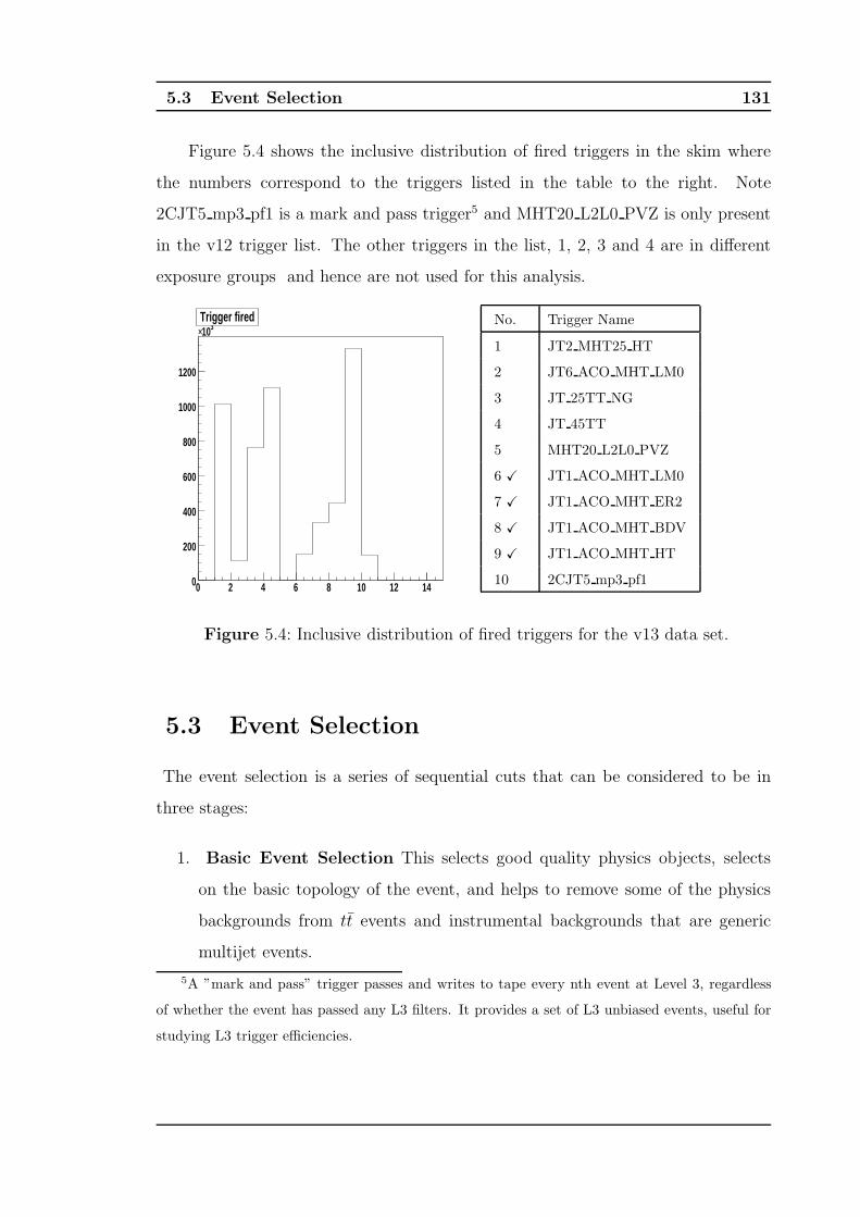
5.3 Event Selection 131
Figure 5.4 shows the inclusive distribution of fired triggers in the skim where
the numbers correspond to the triggers listed in the table to the right. Note
2CJT5 mp3 pf1 is a mark and pass trigger5 and MHT20 L2L0 PVZ is only present
in the v12 trigger list. The other triggers in the list, 1, 2, 3 and 4 are in different
exposure groups and hence are not used for this analysis.
Entries 5402395
Mean 5.217
RMS 3.088Underflow 0
Overflow 0
Integral 5.402e+06
0 2 4 6 8 10 12 140
200
400
600
800
1000
1200
310×
Entries 5402395
Mean 5.217
RMS 3.088Underflow 0
Overflow 0
Integral 5.402e+06Trigger fired No. Trigger Name
1 JT2 MHT25 HT
2 JT6 ACO MHT LM0
3 JT 25TT NG
4 JT 45TT
5 MHT20 L2L0 PVZ
6 X JT1 ACO MHT LM0
7 X JT1 ACO MHT ER2
8 X JT1 ACO MHT BDV
9 X JT1 ACO MHT HT
10 2CJT5 mp3 pf1
Figure 5.4: Inclusive distribution of fired triggers for the v13 data set.
5.3 Event Selection
The event selection is a series of sequential cuts that can be considered to be in
three stages:
1. Basic Event Selection This selects good quality physics objects, selects
on the basic topology of the event, and helps to remove some of the physics
backgrounds from tt events and instrumental backgrounds that are generic
multijet events.
5A ”mark and pass” trigger passes and writes to tape every nth event at Level 3, regardless
of whether the event has passed any L3 filters. It provides a set of L3 unbiased events, useful for
studying L3 trigger efficiencies.
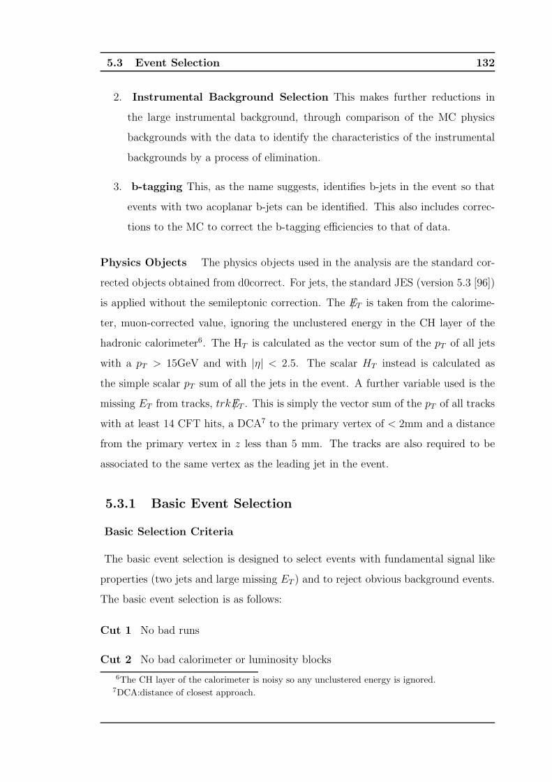
5.3 Event Selection 132
2. Instrumental Background Selection This makes further reductions in
the large instrumental background, through comparison of the MC physics
backgrounds with the data to identify the characteristics of the instrumental
backgrounds by a process of elimination.
3. b-tagging This, as the name suggests, identifies b-jets in the event so that
events with two acoplanar b-jets can be identified. This also includes correc-
tions to the MC to correct the b-tagging efficiencies to that of data.
Physics Objects The physics objects used in the analysis are the standard cor-
rected objects obtained from d0correct. For jets, the standard JES (version 5.3 [96])
is applied without the semileptonic correction. The E/T is taken from the calorime-
ter, muon-corrected value, ignoring the unclustered energy in the CH layer of the
hadronic calorimeter6. The HT is calculated as the vector sum of the pT of all jets
with a pT > 15GeV and with |η| < 2.5. The scalar HT instead is calculated as
the simple scalar pT sum of all the jets in the event. A further variable used is the
missing ET from tracks, trkE/T . This is simply the vector sum of the pT of all tracks
with at least 14 CFT hits, a DCA7 to the primary vertex of < 2mm and a distance
from the primary vertex in z less than 5 mm. The tracks are also required to be
associated to the same vertex as the leading jet in the event.
5.3.1 Basic Event Selection
Basic Selection Criteria
The basic event selection is designed to select events with fundamental signal like
properties (two jets and large missing ET ) and to reject obvious background events.
The basic event selection is as follows:
Cut 1 No bad runs
Cut 2 No bad calorimeter or luminosity blocks
6The CH layer of the calorimeter is noisy so any unclustered energy is ignored.7DCA:distance of closest approach.
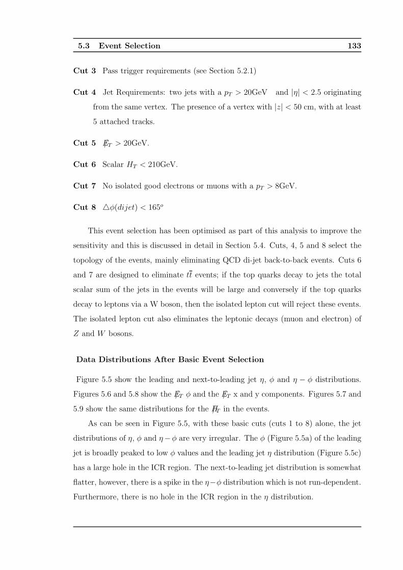
5.3 Event Selection 133
Cut 3 Pass trigger requirements (see Section 5.2.1)
Cut 4 Jet Requirements: two jets with a pT > 20GeV and |η| < 2.5 originating
from the same vertex. The presence of a vertex with |z| < 50 cm, with at least
5 attached tracks.
Cut 5 E/T > 20GeV.
Cut 6 Scalar HT < 210GeV.
Cut 7 No isolated good electrons or muons with a pT > 8GeV.
Cut 8 △φ(dijet) < 165o
This event selection has been optimised as part of this analysis to improve the
sensitivity and this is discussed in detail in Section 5.4. Cuts, 4, 5 and 8 select the
topology of the events, mainly eliminating QCD di-jet back-to-back events. Cuts 6
and 7 are designed to eliminate tt events; if the top quarks decay to jets the total
scalar sum of the jets in the events will be large and conversely if the top quarks
decay to leptons via a W boson, then the isolated lepton cut will reject these events.
The isolated lepton cut also eliminates the leptonic decays (muon and electron) of
Z and W bosons.
Data Distributions After Basic Event Selection
Figure 5.5 show the leading and next-to-leading jet η, φ and η − φ distributions.
Figures 5.6 and 5.8 show the E/T φ and the E/T x and y components. Figures 5.7 and
5.9 show the same distributions for the H/T in the events.
As can be seen in Figure 5.5, with these basic cuts (cuts 1 to 8) alone, the jet
distributions of η, φ and η−φ are very irregular. The φ (Figure 5.5a) of the leading
jet is broadly peaked to low φ values and the leading jet η distribution (Figure 5.5c)
has a large hole in the ICR region. The next-to-leading jet distribution is somewhat
flatter, however, there is a spike in the η−φ distribution which is not run-dependent.
Furthermore, there is no hole in the ICR region in the η distribution.
5.3 Event Selection 134
φLeading jet 0 1 2 3 4 5 6
0
2000
4000
6000
8000
10000
12000
a)a)
φNext to Leading jet 0 1 2 3 4 5 6
0
2000
4000
6000
8000
10000
b)b)
ηLeading jet -2.5 -2 -1.5 -1 -0.5 0 0.5 1 1.5 2 2.50
2000
4000
6000
8000
10000
12000
14000
16000
18000
20000
22000
c)c)
ηNext to Leading jet -2.5 -2 -1.5 -1 -0.5 0 0.5 1 1.5 2 2.50
2000
4000
6000
8000
10000
12000
14000
16000
d)d)
φLeading jet
01 2 3
4 5 6η
Leading jet
-2.5-2-1.5
-1-0.500.5
11.522.5
0
200
400
600
800
1000
e)e)
φNext to Leading jet
01 2 3
4 5 6η
Next to Leading jet
-2.5-2-1.5
-1-0.500.5
11.522.5
0
100
200300
400
500600
700
f)f)
Figure 5.5: Distributions for the leading and next-to-leading jet in the event after
basic cuts. a)φ-distribution for leading jet, b)φ-distribution for next-to leading jet,
c)η-distribution for leading jet, d)η-distribution for next-to leading jet, e)η − φ-
distribution for leading jet and f)η − φ-distribution for next-to leading jet.
All the E/T (Figure 5.6) and H/T (Figure 5.7) distributions are broadly similar
except for the absence of the low tail in the actual E/T distribution (due to the E/T
cut in the basic selection) and in the φ distribution at φ > 5. There are clear
asymmetries in the E/T and H/T distributions, the origins of which are not clear, but
are thought to be the result of a combination of miscalibrations in the calorimeter,
instrumental backgrounds, trigger effects, presence of ”bad” and noise jets in the
event, etc. In addition to this asymmetries in the φ distribution, the x and y-
components show the a dip around zero, characteristic of some of the problems with
DØ tracking. These are beyond the scope of this thesis and are not discussed further
here.
5.3 Event Selection 135
MET0 20 40 60 80 100 120
0
5000
10000
15000
20000
25000
30000
35000
40000
a)a)
φMET 0 1 2 3 4 5 6
0
1000
2000
3000
4000
5000
6000
7000
b)b)
xMET-100 -80 -60 -40 -20 0 20 40 60 80 1000
5000
10000
15000
20000
25000
c)c)
yMET-100 -80 -60 -40 -20 0 20 40 60 80 1000
5000
10000
15000
20000
25000
30000
d)d)
Figure 5.6: E/T distributions after basic cuts and a two-jet requirement. Top left:
E/T Top right: E/T - φ which shows the asymmetry that is thought to be due to
calorimeter miscalibrations, instrumental backgrounds, trigger effects and ’noise’
jets in the event. Bottom left: E/T x-component Bottom right: E/T y-component.
In addition to the asymmetry mentioned visible in the φ distribution, the x and
y-components show the a dip around zero characteristic of some of the problems
with DØ tracking.
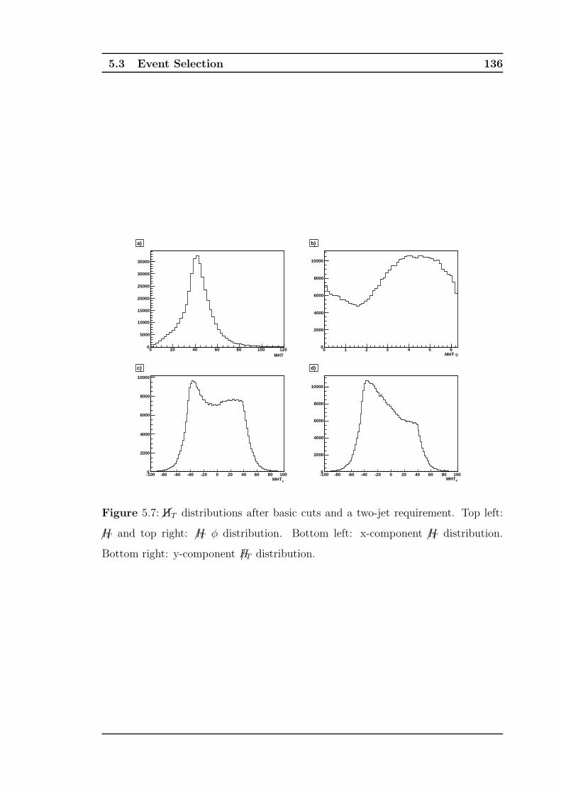
5.3 Event Selection 136
MHT0 20 40 60 80 100 120
0
5000
10000
15000
20000
25000
30000
35000
a)
φMHT 0 1 2 3 4 5 6
0
2000
4000
6000
8000
10000
b)
xMHT-100 -80 -60 -40 -20 0 20 40 60 80 1000
2000
4000
6000
8000
10000
c)
yMHT-100 -80 -60 -40 -20 0 20 40 60 80 1000
2000
4000
6000
8000
10000
d)
Figure 5.7: ��HT distributions after basic cuts and a two-jet requirement. Top left:
H/T and top right: H/T φ distribution. Bottom left: x-component H/T distribution.
Bottom right: y-component H/T distribution.
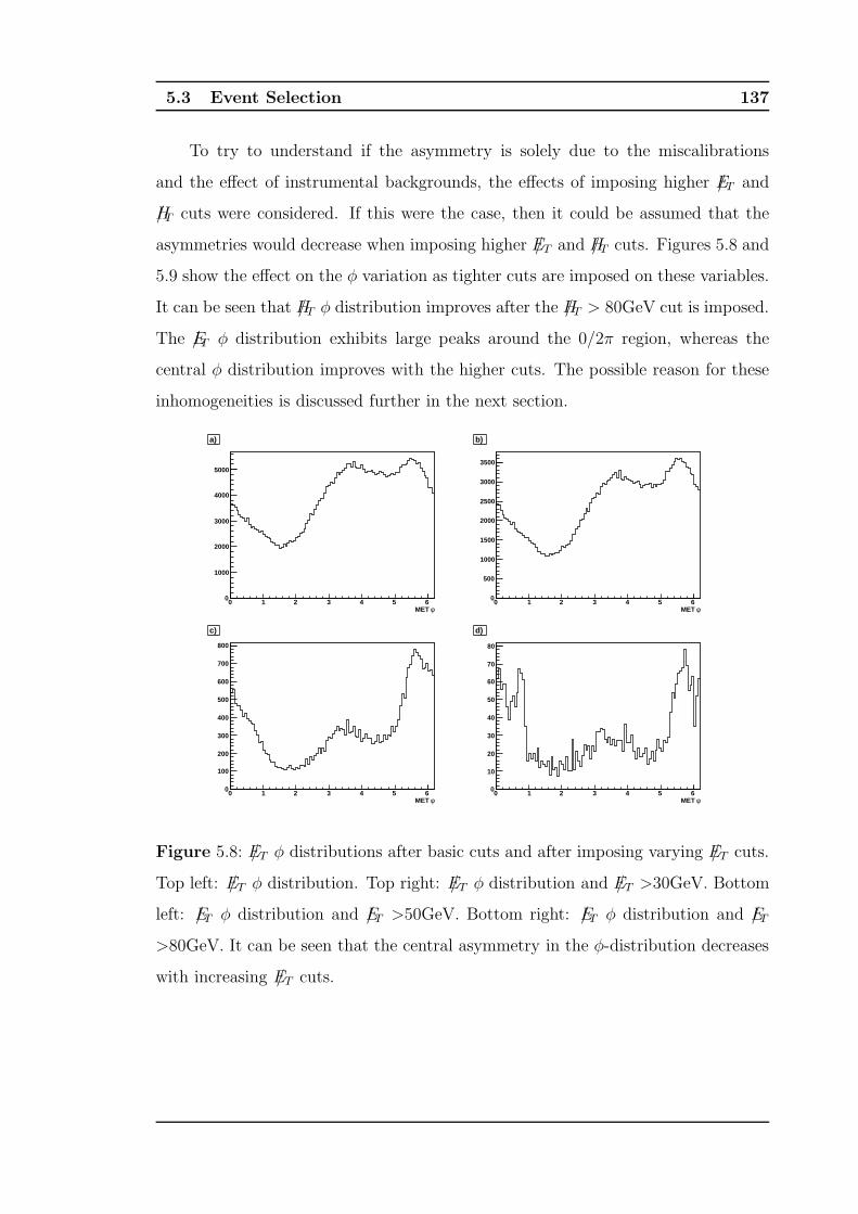
5.3 Event Selection 137
To try to understand if the asymmetry is solely due to the miscalibrations
and the effect of instrumental backgrounds, the effects of imposing higher E/T and
H/T cuts were considered. If this were the case, then it could be assumed that the
asymmetries would decrease when imposing higher E/T and H/T cuts. Figures 5.8 and
5.9 show the effect on the φ variation as tighter cuts are imposed on these variables.
It can be seen that H/T φ distribution improves after the H/T > 80GeV cut is imposed.
The E/T φ distribution exhibits large peaks around the 0/2π region, whereas the
central φ distribution improves with the higher cuts. The possible reason for these
inhomogeneities is discussed further in the next section.
φMET 0 1 2 3 4 5 6
0
1000
2000
3000
4000
5000
a)
φMET 0 1 2 3 4 5 6
0
500
1000
1500
2000
2500
3000
3500
b)
φMET 0 1 2 3 4 5 6
0
100
200
300
400
500
600
700
800
c)
φMET 0 1 2 3 4 5 6
0
10
20
30
40
50
60
70
80
d)
Figure 5.8: E/T φ distributions after basic cuts and after imposing varying E/T cuts.
Top left: E/T φ distribution. Top right: E/T φ distribution and E/T >30GeV. Bottom
left: E/T φ distribution and E/T >50GeV. Bottom right: E/T φ distribution and E/T
>80GeV. It can be seen that the central asymmetry in the φ-distribution decreases
with increasing E/T cuts.
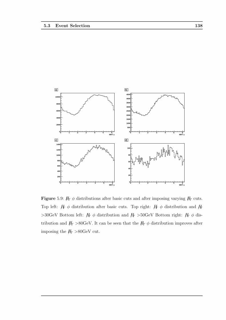
5.3 Event Selection 138
φMHT 0 1 2 3 4 5 6
0
2000
4000
6000
8000
10000
a)
φMHT 0 1 2 3 4 5 6
0
500
1000
1500
2000
2500
3000
3500
4000
4500
b)
φMHT 0 1 2 3 4 5 6
0
200
400
600
800
1000
1200
1400
c)
φMHT 0 1 2 3 4 5 6
0
20
40
60
80
100
d)
Figure 5.9: H/T φ distributions after basic cuts and after imposing varying H/T cuts.
Top left: H/T φ distribution after basic cuts. Top right: H/T φ distribution and H/T
>30GeV Bottom left: H/T φ distribution and H/T >50GeV Bottom right: H/T φ dis-
tribution and H/T >80GeV. It can be seen that the H/T φ distribution improves after
imposing the H/T >80GeV cut.
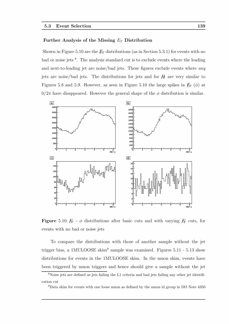
5.3 Event Selection 139
Further Analysis of the Missing ET Distribution
Shown in Figure 5.10 are the E/T distributions (as in Section 5.3.1) for events with no
bad or noise jets 8. The analysis standard cut is to exclude events where the leading
and next-to-leading jet are noise/bad jets. These figures exclude events where any
jets are noise/bad jets. The distributions for jets and for H/T are very similar to
Figures 5.8 and 5.9. However, as seen in Figure 5.10 the large spikes in E/T (φ) at
0/2π have disappeared. However the general shape of the φ distribution is similar.
φMET 0 1 2 3 4 5 6
0
500
1000
1500
2000
2500
3000
3500
4000
a)
φMET 0 1 2 3 4 5 6
0
200
400
600
800
1000
1200
1400
1600
1800
2000
2200
b)
φMET 0 1 2 3 4 5 6
0
20
40
60
80
100
120
140
c)
φMET 0 1 2 3 4 5 6
0
2
4
6
8
10
12
14
16
d)
Figure 5.10: E/T - φ distributions after basic cuts and with varying E/T cuts, for
events with no bad or noise jets
To compare the distributions with those of another sample without the jet
trigger bias, a 1MULOOSE skim9 sample was examined. Figures 5.11 - 5.13 show
distributions for events in the 1MULOOSE skim. In the muon skim, events have
been triggered by muon triggers and hence should give a sample without the jet
8Noise jets are defined as jets failing the L1 criteria and bad jets failing any other jet identifi-
cation cut9Data skim for events with one loose muon as defined by the muon id group in DØ Note 4350

5.3 Event Selection 140
trigger bias and with less QCD background (there should be a large fraction of
W+jet events). To create a E/T signal, any good isolated muons have their momenta
reversed and added to the E/T in the event. Interestingly, for this sample, the leading
jet does not have a hole in the ICR in the η distribution. Furthermore, the jet
φ distributions are a lot flatter although still show similar features. The E/T and
H/T distributions still exhibit a similar structure to the jets from the analysis data
sample. This would really indicate that although a trigger bias accounts for some
of the structure, the major features are trigger-independent and are related to the
features of the hardware or the reconstruction process. Fortunately, it is possible
to impose instrumental cuts to eliminate these inhomogeneities. These cuts are
described in detail in Section 5.3.2.
5.3.2 Instrumental and Other Selection Criteria
To compensate for the differences and the inhomogeneities in the distributions af-
ter the basic event selection, various cuts are imposed to deal with the instrumental
backgrounds which give rise to these asymmetries. For events with a ‘physical origin’
the H/T , E/T and trkE/T should all point in the same direction and should be corre-
lated. Furthermore, di-jet events in which one of the jets has been mis-measured,
so giving a E/T signal, will have the E/T in the same φ-direction as one of the jets.
In the case of trkE/T , this above statement assumes that the fake track distribution
and the tracking efficiency is flat in φ. Following earlier work for the v12 analysis
[90], the cuts below were applied, after those listed in Section 5.3.1. These cuts are
motivated and explained following their listing:
Cut 9 min∆φ(E/T , jets) > 0.15
Cut 10 E/T > −40 ×min∆φ(E/T , jets) + 80GeV
Cut 11 ∆φ(E/T , trkE/T ) < 1.0
Cut 12 0 < Asym(E/T , trkE/T ) < 0.6, where Asym(E/T , trkH/T ) ≡ (E/T−trkE/T )/(E/T+
trkE/T ) < 0.6
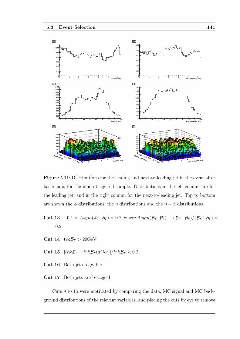
5.3 Event Selection 141
φLeading jet 0 1 2 3 4 5 60
200
400
600
800
1000
1200
a)
φNext to Leading jet 0 1 2 3 4 5 60
200
400
600
800
1000
1200
b)
ηLeading jet -2.5 -2 -1.5 -1 -0.5 0 0.5 1 1.5 2 2.50
200
400
600
800
1000
1200
1400
1600
1800
2000
2200
2400
c)
ηNext to Leading jet -2.5 -2 -1.5 -1 -0.5 0 0.5 1 1.5 2 2.50
200
400
600
800
1000
1200
1400
1600
1800
d)
φLeading jet
0 1 2 3 4 5 6η
Leading jet
-2.5-2-1.5-1
-0.500.511.52
2.50
20
40
60
80
100
120
e)
φNext to Leading jet
0 1 2 3 4 5 6
η
Next to Leading jet -2.5-2
-1.5-1-0.500.51
1.522.5
01020304050607080
f)
Figure 5.11: Distributions for the leading and next-to-leading jet in the event after
basic cuts, for the muon-triggered sample. Distributions in the left column are for
the leading jet, and in the right column for the next-to-leading jet. Top to bottom
are shown the φ distributions, the η distributions and the η − φ distributions.
Cut 13 −0.1 < Asym(E/T , H/T ) < 0.2, where Asym(E/T , H/T ) ≡ (E/T−H/T )/(E/T+H/T ) <
0.2
Cut 14 trkE/T > 20GeV
Cut 15 |trkE/T − trkE/T (dijet)|/trkE/T < 0.2
Cut 16 Both jets taggable
Cut 17 Both jets are b-tagged
Cuts 9 to 15 were motivated by comparing the data, MC signal and MC back-
ground distributions of the relevant variables, and placing the cuts by eye to remove
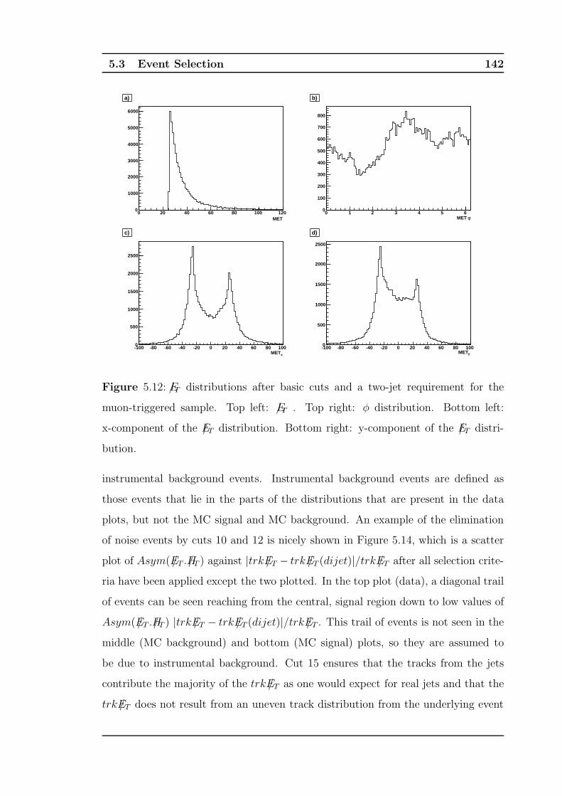
5.3 Event Selection 142
MET0 20 40 60 80 100 120
0
1000
2000
3000
4000
5000
6000
a)
φMET 0 1 2 3 4 5 6
0
100
200
300
400
500
600
700
800
b)
xMET-100 -80 -60 -40 -20 0 20 40 60 80 1000
500
1000
1500
2000
2500
c)
yMET-100 -80 -60 -40 -20 0 20 40 60 80 1000
500
1000
1500
2000
2500
d)
Figure 5.12: E/T distributions after basic cuts and a two-jet requirement for the
muon-triggered sample. Top left: E/T . Top right: φ distribution. Bottom left:
x-component of the E/T distribution. Bottom right: y-component of the E/T distri-
bution.
instrumental background events. Instrumental background events are defined as
those events that lie in the parts of the distributions that are present in the data
plots, but not the MC signal and MC background. An example of the elimination
of noise events by cuts 10 and 12 is nicely shown in Figure 5.14, which is a scatter
plot of Asym(E/T .H/T ) against |trkE/T − trkE/T (dijet)|/trkE/T after all selection crite-
ria have been applied except the two plotted. In the top plot (data), a diagonal trail
of events can be seen reaching from the central, signal region down to low values of
Asym(E/T .H/T ) |trkE/T − trkE/T (dijet)|/trkE/T . This trail of events is not seen in the
middle (MC background) and bottom (MC signal) plots, so they are assumed to
be due to instrumental background. Cut 15 ensures that the tracks from the jets
contribute the majority of the trkE/T as one would expect for real jets and that the
trkE/T does not result from an uneven track distribution from the underlying event
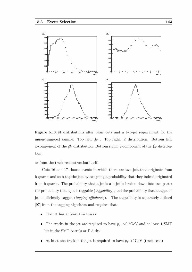
5.3 Event Selection 143
MHT0 20 40 60 80 100 120
0
500
1000
1500
2000
2500
3000
a)
φMHT 0 1 2 3 4 5 6
0
200
400
600
800
1000
1200
1400
b)
xMHT-100 -80 -60 -40 -20 0 20 40 60 80 1000
200
400
600
800
1000
1200
1400
1600
1800
2000
c)
yMHT-100 -80 -60 -40 -20 0 20 40 60 80 1000
200
400
600
800
1000
1200
1400
1600
1800
2000
2200
d)
Figure 5.13: H/T distributions after basic cuts and a two-jet requirement for the
muon-triggered sample. Top left: H/T . Top right: φ distribution. Bottom left:
x-component of the H/T distribution. Bottom right: y-component of the H/T distribu-
tion.
or from the track reconstruction itself.
Cuts 16 and 17 choose events in which there are two jets that originate from
b-quarks and so b-tag the jets by assigning a probability that they indeed originated
from b-quarks. The probability that a jet is a b-jet is broken down into two parts:
the probability that a jet is taggable (taggability), and the probability that a taggable
jet is efficiently tagged (tagging efficiency). The taggability is separately defined
[97] from the tagging algorithm and requires that:
• The jet has at least two tracks.
• The tracks in the jet are required to have pT >0.5GeV and at least 1 SMT
hit in the SMT barrels or F disks
• At least one track in the jet is required to have pT >1GeV (track seed)

5.3 Event Selection 144
• Tracks are required to have DCA<0.2cm and ZDCA <0.4cm.
A priori, it is expected that taggability will be different between data and Monte
Carlo. In MC, the taggability is higher than in data mainly due to a limited descrip-
tion of the tracking detectors resulting in a higher tracking efficiency, particularly
within jets. So the MC taggability must be calibrated to that observed in the data
and this process is described in Section 5.3.4.
5.3.3 Background Estimation
By applying the cuts outlined in the previous section, the instrumental background
is reduced significantly. However, the absolute scale of this background, which is
mainly QCD, is still unknown. It is difficult to model the scale of the QCD back-
ground accurately in Monte Carlo so the normalisation is estimated by selecting
a region of parameter space (the sideband region) which is expected to be dom-
inated by the QCD background. The parameter space chosen was Asym(E/T , H/T )
against |trkE/T − trkE/T (dijet)|/trkE/T because the signal, physics and instrumental
background events are visibly separate. The distributions for signal, MC physics
backgrounds and data are shown in Figure 5.14. The scatter plots have been divided
into three boxes, a central ‘signal’ box (cuts 10 and 12) and two sideband regions
defined by 0.4 > (E/T +H/T )/dijet(trkE/T ) < 1.0 and −0.1 < Asym(E/T , H/T ) < 0.2.
Examining Figure 5.14, the central region well defines the signal events, contains
physics background events, and excludes the instrumental background events. The
sidebands include and exclude the opposite, so they may be used to make a good
estimate, by extrapolation, of the number of unwanted ‘QCD’ events in the signal
region. The MC shape is calculated via a fit to MC events in the signal box whereas
that of the instrumental background is calculated from a fit to data in the sideband
regions. The absolute normalisation of the MC and the instrumental background is
then fixed via the combined fit of the two to the data in the signal box, allowing
only the absolute scale of the two backgrounds to float.
Figure 5.15 shows the fits to the physics background, sideband data and the
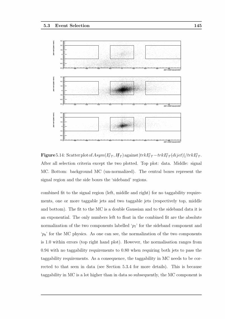
5.3 Event Selection 145
(MET-trkMET(dijet))/trkMET-1 -0.8 -0.6 -0.4 -0.2 0 0.2 0.4 0.6 0.8 1
(ME
T-M
HT
)/(M
ET
+MH
T)
-0.3
-0.2
-0.1
0
0.1
0.2
0.3
(MET-trkMET(dijet))/trkMET-1 -0.8 -0.6 -0.4 -0.2 0 0.2 0.4 0.6 0.8 1
(ME
T-M
HT
)/(M
ET
+MH
T)
-0.3
-0.2
-0.1
0
0.1
0.2
0.3
(MET-trkMET(dijet))/trkMET-1 -0.8 -0.6 -0.4 -0.2 0 0.2 0.4 0.6 0.8 1
(ME
T-M
HT
)/(M
ET
+MH
T)
-0.3
-0.2
-0.1
0
0.1
0.2
0.3
Figure5.14: ScatterplotofAsym(E/T , H/T )against |trkE/T −trkE/T (dijet)|/trkE/T .
After all selection criteria except the two plotted. Top plot: data. Middle: signal
MC. Bottom: background MC (un-normalized). The central boxes represent the
signal region and the side boxes the ‘sideband’ regions.
combined fit to the signal region (left, middle and right) for no taggability require-
ments, one or more taggable jets and two taggable jets (respectively top, middle
and bottom). The fit to the MC is a double Gaussian and to the sideband data it is
an exponential. The only numbers left to float in the combined fit are the absolute
normalization of the two components labelled ‘p7’ for the sideband component and
‘p8’ for the MC physics. As one can see, the normalization of the two components
is 1.0 within errors (top right hand plot). However, the normalisation ranges from
0.94 with no taggability requirements to 0.80 when requiring both jets to pass the
taggability requirements. As a consequence, the taggability in MC needs to be cor-
rected to that seen in data (see Section 5.3.4 for more details). This is because
taggability in MC is a lot higher than in data so subsequently, the MC component is
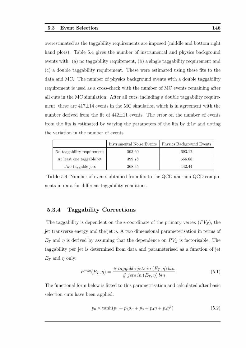
5.3 Event Selection 146
overestimated as the taggability requirements are imposed (middle and bottom right
hand plots). Table 5.4 gives the number of instrumental and physics background
events with: (a) no taggability requirement, (b) a single taggability requirement and
(c) a double taggability requirement. These were estimated using these fits to the
data and MC. The number of physics background events with a double taggability
requirement is used as a cross-check with the number of MC events remaining after
all cuts in the MC simulation. After all cuts, including a double taggability require-
ment, these are 417±14 events in the MC simulation which is in agreement with the
number derived from the fit of 442±11 events. The error on the number of events
from the fits is estimated by varying the parameters of the fits by ±1σ and noting
the variation in the number of events.
Instrumental Noise Events Physics Background Events
No taggability requirement 593.60 693.12
At least one taggable jet 399.78 656.68
Two taggable jets 268.35 442.44
Table 5.4: Number of events obtained from fits to the QCD and non-QCD compo-
nents in data for different taggability conditions.
5.3.4 Taggability Corrections
The taggability is dependent on the z-coordinate of the primary vertex (PVZ), the
jet transverse energy and the jet η. A two dimensional parameterisation in terms of
ET and η is derived by assuming that the dependence on PVZ is factorisable. The
taggability per jet is determined from data and parameterised as a function of jet
ET and η only:
P tagg(ET , η) =# taggable jets in (ET , η) bin
# jets in (ET , η) bin. (5.1)
The functional form below is fitted to this parametrisation and calculated after basic
selection cuts have been applied:
p0 × tanh(p1 + p2pT + p3 + p4η + p4η2) (5.2)
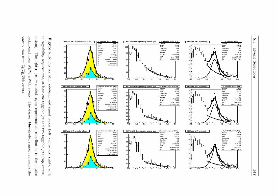
5.3
Event
Sele
ctio
n147
h_metmht_asym_allmcEntries 24445Mean 0.006606
RMS 0.06757
Underflow 0.8523Overflow 0.6106Integral 798.5
/ ndf 2χ 49.84 / 63Prob 0.886
p0 4.40± 27.24
p1 0.002082± 0.005903 p2 0.00236± 0.06426
p3 5.01± 26.71
p4 0.0051± 0.0303
-0.3 -0.2 -0.1 0 0.1 0.2 0.30
10
20
30
40
50
60
h_metmht_asym_allmcEntries 24445Mean 0.006606
RMS 0.06757
Underflow 0.8523Overflow 0.6106Integral 798.5
/ ndf 2χ 49.84 / 63Prob 0.886
p0 4.40± 27.24
p1 0.002082± 0.005903 p2 0.00236± 0.06426
p3 5.01± 26.71
p4 0.0051± 0.0303
MET and MHT asymmetry for all mc h_metmht_asym_qcdEntries 3176Mean -0.145RMS 0.1241Underflow 687Overflow 97Integral 2392
/ ndf 2χ 43.43 / 33Prob 0.1059p0 0.82± 20.16 p1 0.468± -7.044
-0.3 -0.2 -0.1 0 0.1 0.2 0.30
20
40
60
80
100
h_metmht_asym_qcdEntries 3176Mean -0.145RMS 0.1241Underflow 687Overflow 97Integral 2392
/ ndf 2χ 43.43 / 33Prob 0.1059p0 0.82± 20.16 p1 0.468± -7.044
MET and MHT asymmetry for qcd type h_metmht_asymEntries 3707Mean -0.0962RMS 0.1359Underflow 481Overflow 108Integral 3118
/ ndf 2χ 45.05 / 33Prob 0.07879p7 0.084± 1.037 p8 0.071± 0.985
-0.3 -0.2 -0.1 0 0.1 0.2 0.3
10
20
30
40
50
60
70
80
90
h_metmht_asymEntries 3707Mean -0.0962RMS 0.1359Underflow 481Overflow 108Integral 3118
/ ndf 2χ 45.05 / 33Prob 0.07879p7 0.084± 1.037 p8 0.071± 0.985
MET and MHT asymmetry
h_metmht_asym_1tag_allmcEntries 23625
Mean 0.006793
RMS 0.06761Underflow 0.8523
Overflow 0.6097Integral 781.7
/ ndf 2χ 47.79 / 63
Prob 0.9224
p0 4.29± 27.08 p1 0.002095± 0.006133
p2 0.0024± 0.0642
p3 4.91± 26.06 p4 0.00527± 0.02957
-0.3 -0.2 -0.1 0 0.1 0.2 0.30
10
20
30
40
50
60
h_metmht_asym_1tag_allmcEntries 23625
Mean 0.006793
RMS 0.06761Underflow 0.8523
Overflow 0.6097Integral 781.7
/ ndf 2χ 47.79 / 63
Prob 0.9224
p0 4.29± 27.08 p1 0.002095± 0.006133
p2 0.0024± 0.0642
p3 4.91± 26.06 p4 0.00527± 0.02957
MET and MHT asym for all mc h_metmht_asym_qcd_1tagEntries 2726Mean -0.1552RMS 0.125Underflow 650Overflow 84Integral 1992
/ ndf 2χ 37.03 / 33Prob 0.2882p0 0.67± 13.45 p1 0.551± -5.413
-0.3 -0.2 -0.1 0 0.1 0.2 0.30
10
20
30
40
50
60
70
80
90
h_metmht_asym_qcd_1tagEntries 2726Mean -0.1552RMS 0.125Underflow 650Overflow 84Integral 1992
/ ndf 2χ 37.03 / 33Prob 0.2882p0 0.67± 13.45 p1 0.551± -5.413
MET and MHT asymmetry for qcd type h_metmht_asym_1tagEntries 3481Mean -0.09654RMS 0.1371Underflow 452Overflow 106Integral 2923
/ ndf 2χ 40.73 / 33Prob 0.167p7 0.12± 1.42 p8 0.0713± 0.9441
-0.3 -0.2 -0.1 0 0.1 0.2 0.3
10
20
30
40
50
60
70
80
90
h_metmht_asym_1tagEntries 3481Mean -0.09654RMS 0.1371Underflow 452Overflow 106Integral 2923
/ ndf 2χ 40.73 / 33Prob 0.167p7 0.12± 1.42 p8 0.0713± 0.9441
MET and MHT asymmetry
h_metmht_asym_2tag_allmcEntries 21535
Mean 0.008732RMS 0.0684
Underflow 0.8483
Overflow 0.3084Integral 610.6
/ ndf 2χ 43.75 / 62
Prob 0.9619p0 4.92± 28.54
p1 0.002144± 0.008681
p2 0.00297± 0.05744 p3 5.15± 18.31
p4 0.01117± 0.01633
-0.3 -0.2 -0.1 0 0.1 0.2 0.30
10
20
30
40
50
h_metmht_asym_2tag_allmcEntries 21535
Mean 0.008732RMS 0.0684
Underflow 0.8483
Overflow 0.3084Integral 610.6
/ ndf 2χ 43.75 / 62
Prob 0.9619p0 4.92± 28.54
p1 0.002144± 0.008681
p2 0.00297± 0.05744 p3 5.15± 18.31
p4 0.01117± 0.01633
MET and MHT asym for all mc h_metmht_asym_qcd_2tagEntries 2050Mean -0.1627RMS 0.1213Underflow 503Overflow 60Integral 1487
/ ndf 2χ 27.58 / 33Prob 0.7338p0 0.542± 8.793 p1 0.727± -5.448
-0.3 -0.2 -0.1 0 0.1 0.2 0.30
10
20
30
40
50
60
70
h_metmht_asym_qcd_2tagEntries 2050Mean -0.1627RMS 0.1213Underflow 503Overflow 60Integral 1487
/ ndf 2χ 27.58 / 33Prob 0.7338p0 0.542± 8.793 p1 0.727± -5.448
MET and MHT asymmetry for qcd type h_metmht_asym_2tagEntries 2470Mean -0.1009RMS 0.1363Underflow 319Overflow 81Integral 2070
/ ndf 2χ 40.69 / 33Prob 0.168p7 0.151± 1.475 p8 0.0735± 0.8029
-0.3 -0.2 -0.1 0 0.1 0.2 0.30
10
20
30
40
50
60
70
h_metmht_asym_2tagEntries 2470Mean -0.1009RMS 0.1363Underflow 319Overflow 81Integral 2070
/ ndf 2χ 40.69 / 33Prob 0.168p7 0.151± 1.475 p8 0.0735± 0.8029
MET and MHT asymmetry
Fig
ure
5.15:Fits
forM
C,
sideb
and
and
signal
region(left,
centre
and
right),
with
no
taggability
requirem
ents,
atleast
one
taggable
jetan
dtw
otaggab
lejets
(top,cen
tre,
bottom
).T
he
lighter,
yellow-sh
aded
regionrep
resents
the
contrib
ution
toth
ephysics
back
ground
fromW
j/Wjj/W
bb
events.
The
darker,
blu
e-shad
edregion
represen
tsth
e
contrib
ution
fromZj/Z
jj/Zbb
events.
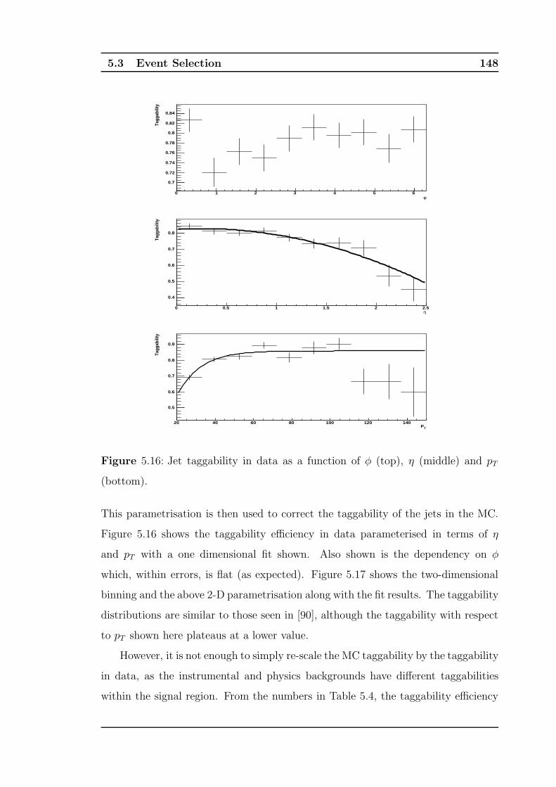
5.3 Event Selection 148
φ0 1 2 3 4 5 6
Tagg
abili
ty
0.7
0.72
0.74
0.76
0.78
0.8
0.82
0.84
η0 0.5 1 1.5 2 2.5
Tagg
abili
ty
0.4
0.5
0.6
0.7
0.8
TP20 40 60 80 100 120 140
Tagg
abili
ty
0.5
0.6
0.7
0.8
0.9
Figure 5.16: Jet taggability in data as a function of φ (top), η (middle) and pT
(bottom).
This parametrisation is then used to correct the taggability of the jets in the MC.
Figure 5.16 shows the taggability efficiency in data parameterised in terms of η
and pT with a one dimensional fit shown. Also shown is the dependency on φ
which, within errors, is flat (as expected). Figure 5.17 shows the two-dimensional
binning and the above 2-D parametrisation along with the fit results. The taggability
distributions are similar to those seen in [90], although the taggability with respect
to pT shown here plateaus at a lower value.
However, it is not enough to simply re-scale the MC taggability by the taggability
in data, as the instrumental and physics backgrounds have different taggabilities
within the signal region. From the numbers in Table 5.4, the taggability efficiency
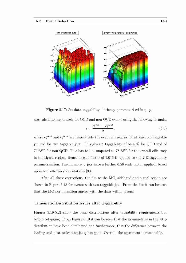
5.3 Event Selection 149
2040
6080
100120
140
0
0.5
1
1.5
2
2.50
0.2
0.4
0.6
0.8
1
h2_jet_eta_pt_tageffEntries 2136Mean x 70.69Mean y 0.9445
RMS x 32.03RMS y 0.6008 0 0 0 0 201 3 0 0 0Integral 201
/ ndf χ 9.688 / 238p0 0.7031± 0.9459 p1 1.602± -0.07105
p2 0.06323± 0.04487 p3 0.6753± 0.8991 p4 0.303± 0.0746 p5 0.1399± -0.07807 p6 0± 1
h2_jet_eta_pt_tageffEntries 2136Mean x 70.69Mean y 0.9445
RMS x 32.03RMS y 0.6008 0 0 0 0 201 3 0 0 0Integral 201
/ ndf χ 9.688 / 238p0 0.7031± 0.9459 p1 1.602± -0.07105
p2 0.06323± 0.04487 p3 0.6753± 0.8991 p4 0.303± 0.0746 p5 0.1399± -0.07807 p6 0± 1
eta phi after all cuts
2040
6080
100120
140
0
0.5
1
1.5
2
2.50.4
0.5
0.6
0.7
0.8
0.9
([6]*([0]*tanh([1]+x*[2])*([3]+[4]*y+[5]*(y*y))))
Figure 5.17: Jet data taggability efficiency parameterised in η−pT
was calculated separately for QCD and non-QCD events using the following formula:
ǫ =ǫevent1 + ǫevent
2
2, (5.3)
where ǫevent1 and ǫevent
2 are respectively the event efficiencies for at least one taggable
jet and for two taggable jets. This gives a taggability of 54.48% for QCD and of
79.63% for non-QCD. This has to be compared to 78.33% for the overall efficiency
in the signal region. Hence a scale factor of 1.016 is applied to the 2-D taggability
parametrisation. Furthermore, τ jets have a further 0.56 scale factor applied, based
upon MC efficiency calculations [90].
After all these corrections, the fits to the MC, sideband and signal region are
shown in Figure 5.18 for events with two taggable jets. From the fits it can be seen
that the MC normalisation agrees with the data within errors.
Kinematic Distribution Issues after Taggability
Figures 5.19-5.21 show the basic distributions after taggability requirements but
before b-tagging. From Figure 5.19 it can be seen that the asymmetries in the jet φ
distribution have been eliminated and furthermore, that the difference between the
leading and next-to-leading jet η has gone. Overall, the agreement is reasonable.

5.3
Event
Sele
ctio
n150
h_metmht_asym_2datatag_allmc
Entries 14967
Mean 0.01029
RMS 0.06801
Underflow 0.8483
Overflow 0.4159
Integral 403.4
/ ndf 2χ 53.69 / 62
Prob 0.7648
p0 12.4± -144.4
p1 0.00256± 0.01166
p2 0.00089± 0.05336
p3 12.4± 169.9
p4 0.00085± -0.05239
-0.3 -0.2 -0.1 0 0.1 0.2 0.3
0
5
10
15
20
25
30
h_metmht_asym_2datatag_allmc
Entries 14967
Mean 0.01029
RMS 0.06801
Underflow 0.8483
Overflow 0.4159
Integral 403.4
/ ndf 2χ 53.69 / 62
Prob 0.7648
p0 12.4± -144.4
p1 0.00256± 0.01166
p2 0.00089± 0.05336
p3 12.4± 169.9
p4 0.00085± -0.05239
MET and MHT asym for all mc h_metmht_asym_qcd_2tag
Entries 2050
Mean -0.1627
RMS 0.1213
Underflow 503
Overflow 60
Integral 1487
/ ndf 2χ 27.58 / 33
Prob 0.7338
p0 0.542± 8.793
p1 0.727± -5.448
-0.3 -0.2 -0.1 0 0.1 0.2 0.3
0
10
20
30
40
50
60
70
h_metmht_asym_qcd_2tag
Entries 2050
Mean -0.1627
RMS 0.1213
Underflow 503
Overflow 60
Integral 1487
/ ndf 2χ 27.58 / 33
Prob 0.7338
p0 0.542± 8.793
p1 0.727± -5.448
MET and MHT asymmetry for qcd type h_metmht_asym_2tag
Entries 2470
Mean -0.1009
RMS 0.1363
Underflow 319
Overflow 81
Integral 2070
/ ndf 2χ 48.87 / 33
Prob 0.03704
p7 0.141± 1.667
p8 0.105± 1.108
-0.3 -0.2 -0.1 0 0.1 0.2 0.3
0
10
20
30
40
50
60
70
h_metmht_asym_2tag
Entries 2470
Mean -0.1009
RMS 0.1363
Underflow 319
Overflow 81
Integral 2070
/ ndf 2χ 48.87 / 33
Prob 0.03704
p7 0.141± 1.667
p8 0.105± 1.108
MET and MHT asymmetry
Fig
ure
5.18:Fits
forM
C,sid
eban
dan
dsign
alregion
(left,centre
and
right)
fortw
o
taggable
jetsafter
taggability
corrections.
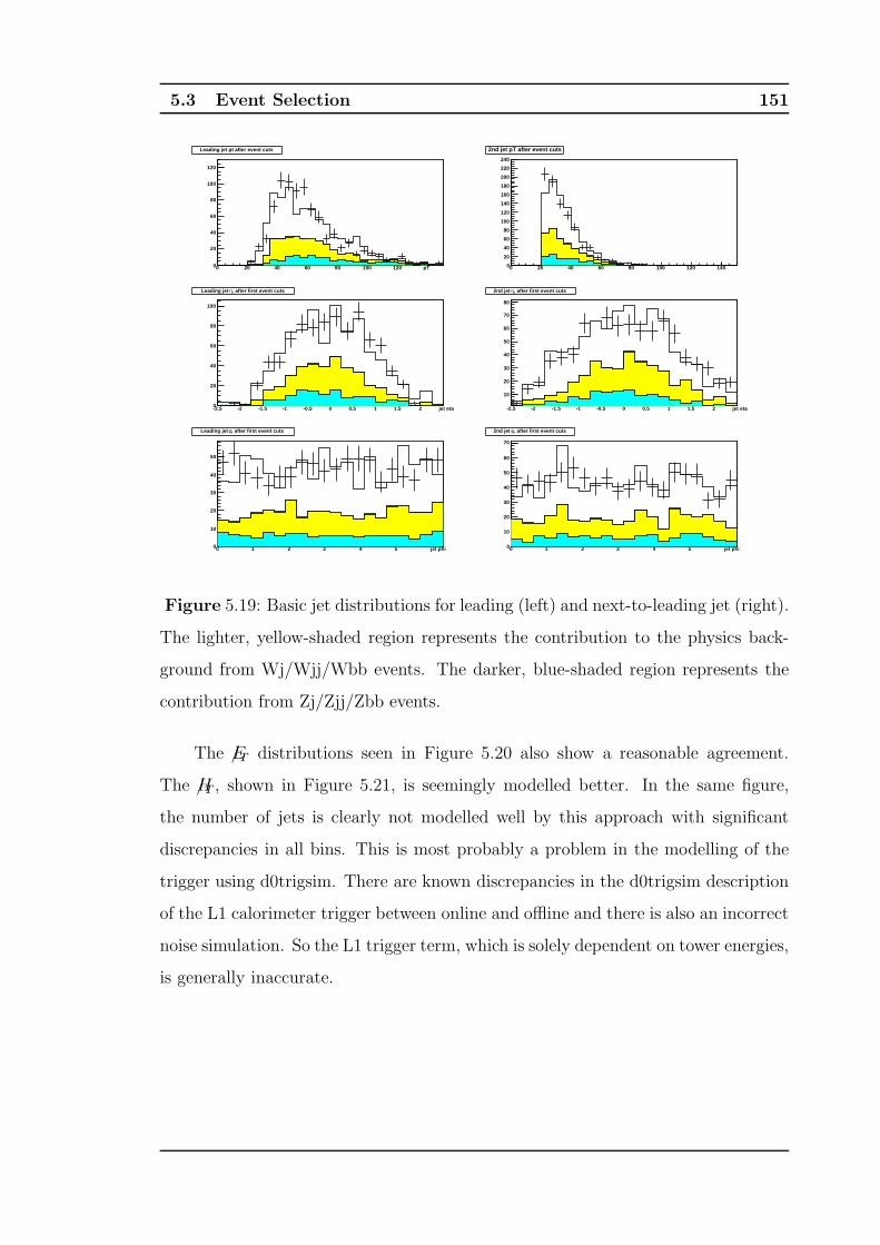
5.3 Event Selection 151
0 20 40 60 80 100 120 pT0
20
40
60
80
100
120
Leading jet pt after event cuts
0 20 40 60 80 100 120 1400
20
40
60
80
100
120
140
160
180
200
220
240
2nd jet pT after event cuts
-2.5 -2 -1.5 -1 -0.5 0 0.5 1 1.5 2 jet eta0
20
40
60
80
100
, after first event cutsηLeading jet
-2.5 -2 -1.5 -1 -0.5 0 0.5 1 1.5 2 jet eta
10
20
30
40
50
60
70
80
, after first event cutsη2nd jet
0 1 2 3 4 5 jet phi0
10
20
30
40
50
, after first event cutsφLeading jet
0 1 2 3 4 5 jet phi0
10
20
30
40
50
60
70
, after first event cutsφ2nd jet
Figure 5.19: Basic jet distributions for leading (left) and next-to-leading jet (right).
The lighter, yellow-shaded region represents the contribution to the physics back-
ground from Wj/Wjj/Wbb events. The darker, blue-shaded region represents the
contribution from Zj/Zjj/Zbb events.
The E/T distributions seen in Figure 5.20 also show a reasonable agreement.
The H/T , shown in Figure 5.21, is seemingly modelled better. In the same figure,
the number of jets is clearly not modelled well by this approach with significant
discrepancies in all bins. This is most probably a problem in the modelling of the
trigger using d0trigsim. There are known discrepancies in the d0trigsim description
of the L1 calorimeter trigger between online and offline and there is also an incorrect
noise simulation. So the L1 trigger term, which is solely dependent on tower energies,
is generally inaccurate.
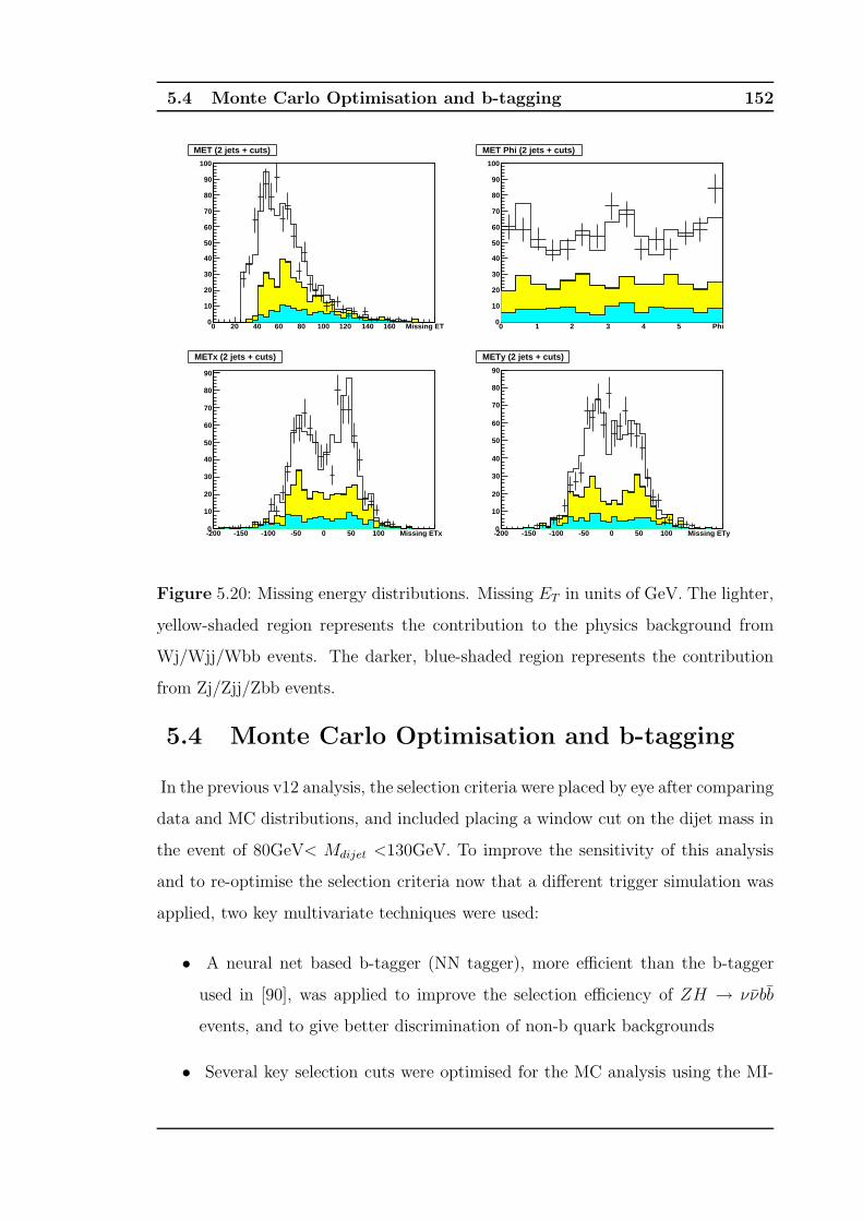
5.4 Monte Carlo Optimisation and b-tagging 152
0 20 40 60 80 100 120 140 160 Missing ET0
10
20
30
40
50
60
70
80
90
100
MET (2 jets + cuts)
0 1 2 3 4 5 Phi0
10
20
30
40
50
60
70
80
90
100
MET Phi (2 jets + cuts)
-200 -150 -100 -50 0 50 100 Missing ETx0
10
20
30
40
50
60
70
80
90
METx (2 jets + cuts)
-200 -150 -100 -50 0 50 100 Missing ETy0
10
20
30
40
50
60
70
80
90
METy (2 jets + cuts)
Figure 5.20: Missing energy distributions. Missing ET in units of GeV. The lighter,
yellow-shaded region represents the contribution to the physics background from
Wj/Wjj/Wbb events. The darker, blue-shaded region represents the contribution
from Zj/Zjj/Zbb events.
5.4 Monte Carlo Optimisation and b-tagging
In the previous v12 analysis, the selection criteria were placed by eye after comparing
data and MC distributions, and included placing a window cut on the dijet mass in
the event of 80GeV< Mdijet <130GeV. To improve the sensitivity of this analysis
and to re-optimise the selection criteria now that a different trigger simulation was
applied, two key multivariate techniques were used:
• A neural net based b-tagger (NN tagger), more efficient than the b-tagger
used in [90], was applied to improve the selection efficiency of ZH → ννbb
events, and to give better discrimination of non-b quark backgrounds
• Several key selection cuts were optimised for the MC analysis using the MI-
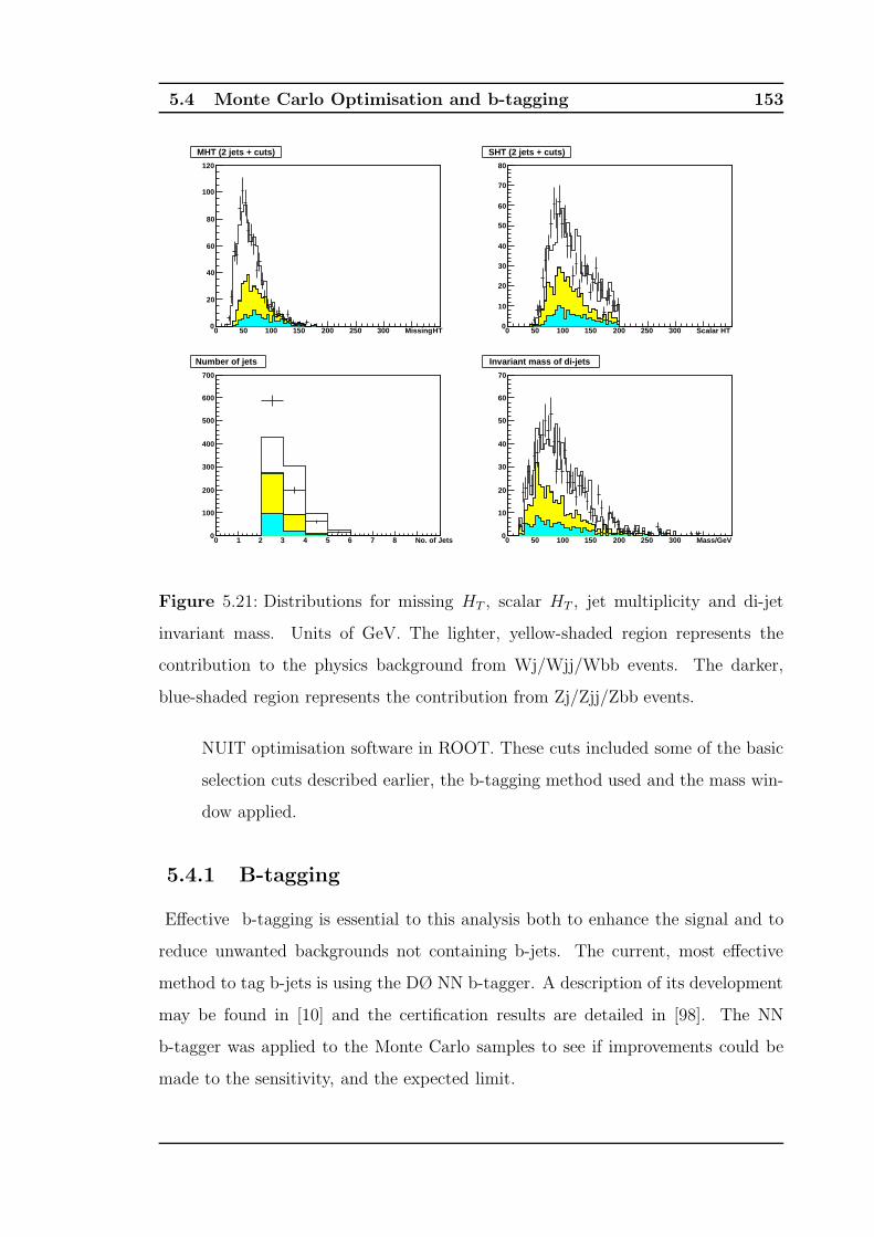
5.4 Monte Carlo Optimisation and b-tagging 153
0 50 100 150 200 250 300 MissingHT0
20
40
60
80
100
120
MHT (2 jets + cuts)
0 50 100 150 200 250 300 Scalar HT0
10
20
30
40
50
60
70
80
SHT (2 jets + cuts)
0 1 2 3 4 5 6 7 8 No. of Jets 0
100
200
300
400
500
600
700
Number of jets
0 50 100 150 200 250 300 Mass/GeV0
10
20
30
40
50
60
70
Invariant mass of di-jets
Figure 5.21: Distributions for missing HT , scalar HT , jet multiplicity and di-jet
invariant mass. Units of GeV. The lighter, yellow-shaded region represents the
contribution to the physics background from Wj/Wjj/Wbb events. The darker,
blue-shaded region represents the contribution from Zj/Zjj/Zbb events.
NUIT optimisation software in ROOT. These cuts included some of the basic
selection cuts described earlier, the b-tagging method used and the mass win-
dow applied.
5.4.1 B-tagging
Effective b-tagging is essential to this analysis both to enhance the signal and to
reduce unwanted backgrounds not containing b-jets. The current, most effective
method to tag b-jets is using the DØ NN b-tagger. A description of its development
may be found in [10] and the certification results are detailed in [98]. The NN
b-tagger was applied to the Monte Carlo samples to see if improvements could be
made to the sensitivity, and the expected limit.
5.4 Monte Carlo Optimisation and b-tagging 154
Other b-taggers Other b-taggers available are the jet lifetime impact parameter
tagger (JLIP)[99], the secondary vertex tagger (SVT)[100] and the counting signed
impact parameter (CSIP) [101] tagger; JLIP is the most effective of the three. All
three are dependent on the long decay path of the B-hadron due to its long lifetime.
The decay of a long-lived hadron produces several charged particles emanating from
a secondary vertex, displaced from the primary pp interaction point.
The JLIP tagger uses the impact parameter information of the tracks seen in
the SMT layers to calculate a probability. The impact parameters of all tracks
associated to a jet can be combined into a single variable called the jet lifetime
probability which is the probability that all tracks in a jet originate from the primary
interaction point. Light quark jets have a flat probability distribution between 0 and
1, whereas the probability distribution for b-jets peaks at a low value so they are
selected by appropriately-placed cuts.
The CSIP b-tagger also relies on the fact that tracks of charged decay products
of long-lived B-hadrons have non-zero impact parameter with respect to the primary
vertex. A sign and significance can be assigned to the impact parameter, and using
these, a jet is tagged if two, or more, tracks associated with this jet have signed
impact parameter significance greater than 3, or three or more tracks have signed
impact parameter significance greater than 2.
The SVT identifies B-hadrons based on the properties of the secondary vertex
and the decay length of the B-hadron. Using Pythia Monte Carlo, the ’average’
properties of a B-hadron secondary vertex are described in terms of the decay length,
the average number of charged particles emanating from the secondary vertex, the jet
cone size containing 99% of the jet energy and the impact parameter significance10.
The Neural Net Tagger The NN b-tagger shows an improvement of between
15% (loosest operating point) and 40% [98] in signal efficiency over the JLIP tagger,
and fake rates reduced by at least one third for a fixed signal efficiency. The NN
tagger is constructed using the ROOT class TMultiLayerPerceptron and takes as
10Impact parameter significance = Distance of closest approach/σ(Distance of closest approach)
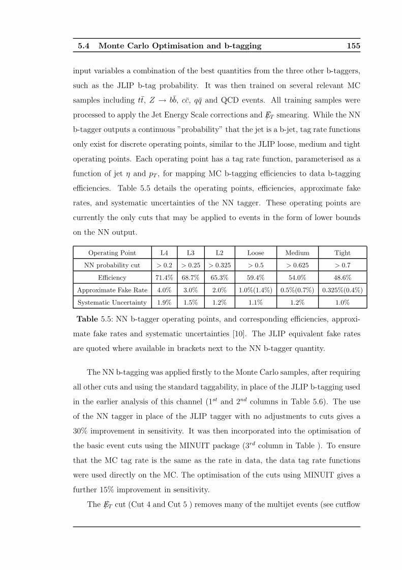
5.4 Monte Carlo Optimisation and b-tagging 155
input variables a combination of the best quantities from the three other b-taggers,
such as the JLIP b-tag probability. It was then trained on several relevant MC
samples including tt, Z → bb, cc, qq and QCD events. All training samples were
processed to apply the Jet Energy Scale corrections and E/T smearing. While the NN
b-tagger outputs a continuous ”probability” that the jet is a b-jet, tag rate functions
only exist for discrete operating points, similar to the JLIP loose, medium and tight
operating points. Each operating point has a tag rate function, parameterised as a
function of jet η and pT , for mapping MC b-tagging efficiencies to data b-tagging
efficiencies. Table 5.5 details the operating points, efficiencies, approximate fake
rates, and systematic uncertainties of the NN tagger. These operating points are
currently the only cuts that may be applied to events in the form of lower bounds
on the NN output.
Operating Point L4 L3 L2 Loose Medium Tight
NN probability cut > 0.2 > 0.25 > 0.325 > 0.5 > 0.625 > 0.7
Efficiency 71.4% 68.7% 65.3% 59.4% 54.0% 48.6%
Approximate Fake Rate 4.0% 3.0% 2.0% 1.0%(1.4%) 0.5%(0.7%) 0.325%(0.4%)
Systematic Uncertainty 1.9% 1.5% 1.2% 1.1% 1.2% 1.0%
Table 5.5: NN b-tagger operating points, and corresponding efficiencies, approxi-
mate fake rates and systematic uncertainties [10]. The JLIP equivalent fake rates
are quoted where available in brackets next to the NN b-tagger quantity.
The NN b-tagging was applied firstly to the Monte Carlo samples, after requiring
all other cuts and using the standard taggability, in place of the JLIP b-tagging used
in the earlier analysis of this channel (1st and 2nd columns in Table 5.6). The use
of the NN tagger in place of the JLIP tagger with no adjustments to cuts gives a
30% improvement in sensitivity. It was then incorporated into the optimisation of
the basic event cuts using the MINUIT package (3rd column in Table ). To ensure
that the MC tag rate is the same as the rate in data, the data tag rate functions
were used directly on the MC. The optimisation of the cuts using MINUIT gives a
further 15% improvement in sensitivity.
The E/T cut (Cut 4 and Cut 5 ) removes many of the multijet events (see cutflow
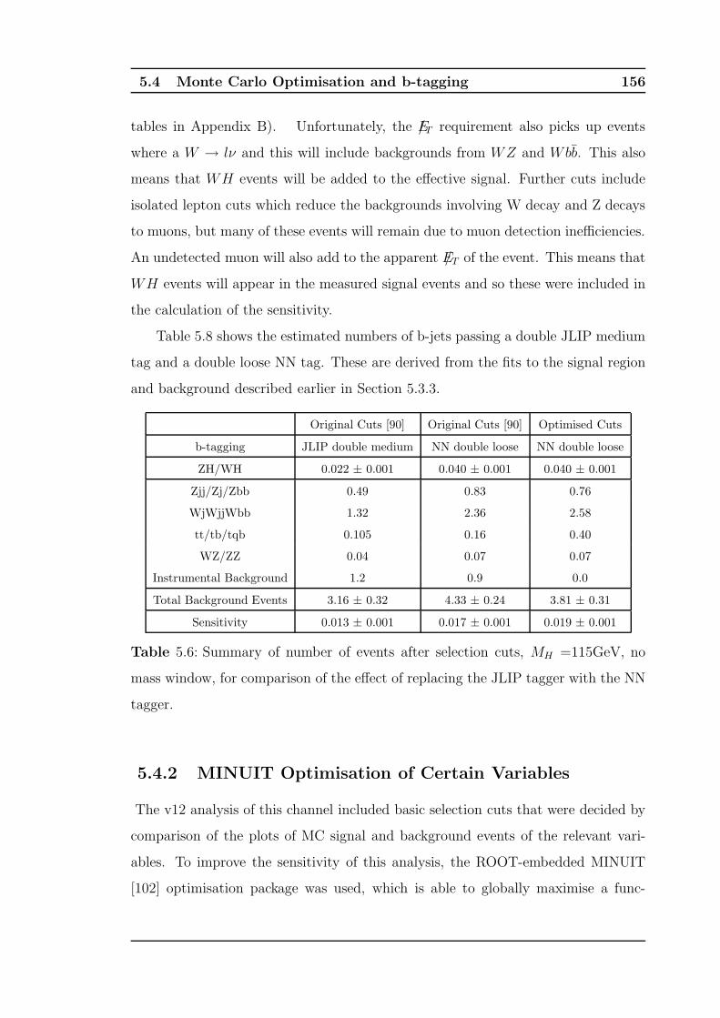
5.4 Monte Carlo Optimisation and b-tagging 156
tables in Appendix B). Unfortunately, the E/T requirement also picks up events
where a W → lν and this will include backgrounds from WZ and Wbb. This also
means that WH events will be added to the effective signal. Further cuts include
isolated lepton cuts which reduce the backgrounds involving W decay and Z decays
to muons, but many of these events will remain due to muon detection inefficiencies.
An undetected muon will also add to the apparent E/T of the event. This means that
WH events will appear in the measured signal events and so these were included in
the calculation of the sensitivity.
Table 5.8 shows the estimated numbers of b-jets passing a double JLIP medium
tag and a double loose NN tag. These are derived from the fits to the signal region
and background described earlier in Section 5.3.3.
Original Cuts [90] Original Cuts [90] Optimised Cuts
b-tagging JLIP double medium NN double loose NN double loose
ZH/WH 0.022 ± 0.001 0.040 ± 0.001 0.040 ± 0.001
Zjj/Zj/Zbb 0.49 0.83 0.76
WjWjjWbb 1.32 2.36 2.58
tt/tb/tqb 0.105 0.16 0.40
WZ/ZZ 0.04 0.07 0.07
Instrumental Background 1.2 0.9 0.0
Total Background Events 3.16 ± 0.32 4.33 ± 0.24 3.81 ± 0.31
Sensitivity 0.013 ± 0.001 0.017 ± 0.001 0.019 ± 0.001
Table 5.6: Summary of number of events after selection cuts, MH =115GeV, no
mass window, for comparison of the effect of replacing the JLIP tagger with the NN
tagger.
5.4.2 MINUIT Optimisation of Certain Variables
The v12 analysis of this channel included basic selection cuts that were decided by
comparison of the plots of MC signal and background events of the relevant vari-
ables. To improve the sensitivity of this analysis, the ROOT-embedded MINUIT
[102] optimisation package was used, which is able to globally maximise a func-
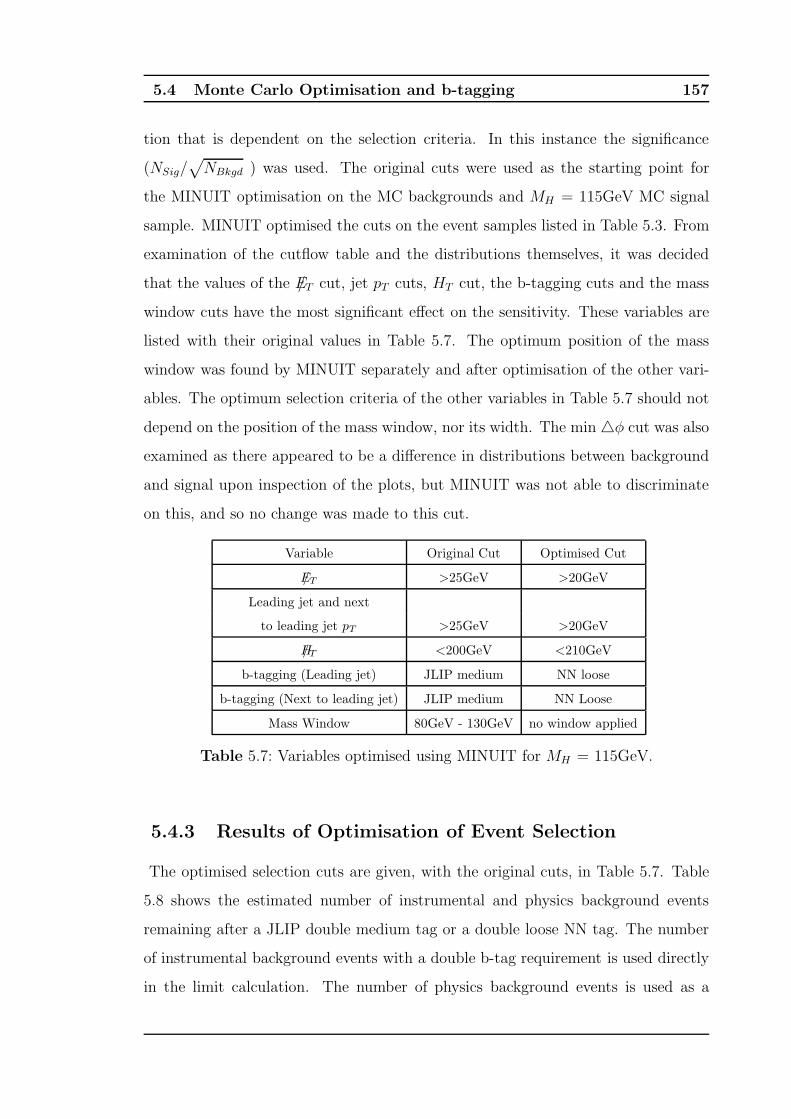
5.4 Monte Carlo Optimisation and b-tagging 157
tion that is dependent on the selection criteria. In this instance the significance
(NSig/√NBkgd ) was used. The original cuts were used as the starting point for
the MINUIT optimisation on the MC backgrounds and MH = 115GeV MC signal
sample. MINUIT optimised the cuts on the event samples listed in Table 5.3. From
examination of the cutflow table and the distributions themselves, it was decided
that the values of the E/T cut, jet pT cuts, HT cut, the b-tagging cuts and the mass
window cuts have the most significant effect on the sensitivity. These variables are
listed with their original values in Table 5.7. The optimum position of the mass
window was found by MINUIT separately and after optimisation of the other vari-
ables. The optimum selection criteria of the other variables in Table 5.7 should not
depend on the position of the mass window, nor its width. The min △φ cut was also
examined as there appeared to be a difference in distributions between background
and signal upon inspection of the plots, but MINUIT was not able to discriminate
on this, and so no change was made to this cut.
Variable Original Cut Optimised Cut
E/T >25GeV >20GeV
Leading jet and next
to leading jet pT >25GeV >20GeV
H/T <200GeV <210GeV
b-tagging (Leading jet) JLIP medium NN loose
b-tagging (Next to leading jet) JLIP medium NN Loose
Mass Window 80GeV - 130GeV no window applied
Table 5.7: Variables optimised using MINUIT for MH = 115GeV.
5.4.3 Results of Optimisation of Event Selection
The optimised selection cuts are given, with the original cuts, in Table 5.7. Table
5.8 shows the estimated number of instrumental and physics background events
remaining after a JLIP double medium tag or a double loose NN tag. The number
of instrumental background events with a double b-tag requirement is used directly
in the limit calculation. The number of physics background events is used as a

5.5 Errors 158
cross-check with the numbers remaining after selection cuts.
Double Taggable JLIP medium double tag NN loose double tag
Physics Background 437.9 2.05 3.05
Instrumental Background 268 1.2 0
Table 5.8: Estimation of the number of instrumental background events after dou-
ble medium JLIP tagging and double loose NN tagging.
5.4.4 Summary of Event Selection
Tables B.1 to B.4 in Appendix B give the selection efficiencies for data, MC signal
and MC backgrounds in percent after optimised cuts, and NN b-tagging. These
detailed tables are summarised later in Table 5.10.
5.5 Errors
The systematic errors for this analysis follow those from the v12 analysis [90] and
are summarized in Table 5.9. It is assumed that the sources of these errors are
uncorrelated and so they have been combined in quadrature. These errors arise
from the errors in the fits used to derive the corrections that have been applied to
the MC samples to correct for the MC/data differences.
These errors were estimated by varying each source of error by ±1σ from the cen-
tral value, and noting how the total background and signal acceptances are changed.
The errors arising from jet corrections (errors 1 to 3 below) are taken directly from
[90] and are assumed to be applicable to this analysis as they apply to the same sam-
ples, the remainder have been calculated as they are more affected by the differences
between the v12 and v13 analyses.
1. Jet Identification Efficiency The jet-id correction factor was varied by
±1σ or 5%, the error on the reconstruction efficiency[76].
2. Jet Energy Scale Factor The correction factor was varied by ±1σ for each
jet. The jet energy correction factor is based on light jets so the difference
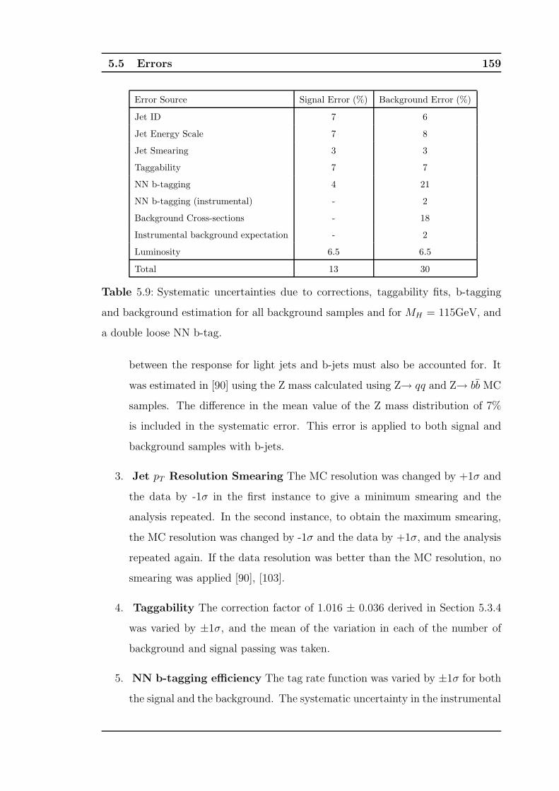
5.5 Errors 159
Error Source Signal Error (%) Background Error (%)
Jet ID 7 6
Jet Energy Scale 7 8
Jet Smearing 3 3
Taggability 7 7
NN b-tagging 4 21
NN b-tagging (instrumental) - 2
Background Cross-sections - 18
Instrumental background expectation - 2
Luminosity 6.5 6.5
Total 13 30
Table 5.9: Systematic uncertainties due to corrections, taggability fits, b-tagging
and background estimation for all background samples and for MH = 115GeV, and
a double loose NN b-tag.
between the response for light jets and b-jets must also be accounted for. It
was estimated in [90] using the Z mass calculated using Z→ qq and Z→ bb MC
samples. The difference in the mean value of the Z mass distribution of 7%
is included in the systematic error. This error is applied to both signal and
background samples with b-jets.
3. Jet pT Resolution Smearing The MC resolution was changed by +1σ and
the data by -1σ in the first instance to give a minimum smearing and the
analysis repeated. In the second instance, to obtain the maximum smearing,
the MC resolution was changed by -1σ and the data by +1σ, and the analysis
repeated again. If the data resolution was better than the MC resolution, no
smearing was applied [90], [103].
4. Taggability The correction factor of 1.016 ± 0.036 derived in Section 5.3.4
was varied by ±1σ, and the mean of the variation in each of the number of
background and signal passing was taken.
5. NN b-tagging efficiency The tag rate function was varied by ±1σ for both
the signal and the background. The systematic uncertainty in the instrumental

5.6 Limit on σ(pp→ ZH) × Br(H → bb) 160
and physics backgrounds was taken from [98] as described in Section 5.4 and
weighted by the assumed ratios of b, c and light-quark jets.
6. Background Cross-sections From comparisons of LO and NLO cross-
sections, this was estimated in the v12 analysis [90] to be a conservative 20%,
leading to an error of 18% in the total background expectation in this analysis.
This is based on information from [8].
7. Instrumental Background Expectation The uncertainty in the instru-
mental background expectation was estimated from the error of the fit to the
backgrounds as described in Section 5.3.2. The error on the fit leads to esti-
mated uncertainties of 268±9 QCD events, and 442±11 physics background
events translating to an error of 2% in the total background.
The statistical errors for the MC signal and background are assumed to be
Poisson-distributed. They are given next to the quantities in the relevant tables.
5.6 Limit on σ(pp→ ZH) ×Br(H → bb)
Upper limits were set for σ(pp→ ZH)×Br(H → bb), for four Higgs boson masses
of 105GeV, 115GeV, 125GeV and 135GeV and are given in Table 5.10. This table
details the number of MC signal events, the number of MC background events and
the number of data events passing all cuts, and the sensitivity of this analysis for
each mass point. Since the background samples used were the same, irrespective of
the Higgs samples used, the number of events for each background does not vary
with the Higgs mass. The table gives the signal acceptance after scaling by the
Z → νν branching ratio of 20% [8]. The 95% C.L. limits are calculated using a
Bayesian method [104] [105] and are found to be between 19.3pb and 57.1pb. The
expected cross-section limits in the no-signal hypothesis were calculated assuming
that Nsig ≪ Nbkg, and that Ndata = Nbkg and were found to be between 13.8pb and
40.3pb. The limits calculated include both the statistical and systematic errors as
calculated and discussed in section 5.5. Figure 5.23 shows one of the five remaining
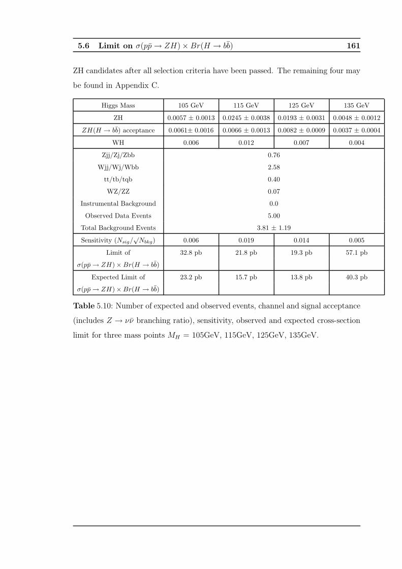
5.6 Limit on σ(pp→ ZH) × Br(H → bb) 161
ZH candidates after all selection criteria have been passed. The remaining four may
be found in Appendix C.
Higgs Mass 105 GeV 115 GeV 125 GeV 135 GeV
ZH 0.0057 ± 0.0013 0.0245 ± 0.0038 0.0193 ± 0.0031 0.0048 ± 0.0012
ZH(H → bb) acceptance 0.0061± 0.0016 0.0066 ± 0.0013 0.0082 ± 0.0009 0.0037 ± 0.0004
WH 0.006 0.012 0.007 0.004
Zjj/Zj/Zbb 0.76
Wjj/Wj/Wbb 2.58
tt/tb/tqb 0.40
WZ/ZZ 0.07
Instrumental Background 0.0
Observed Data Events 5.00
Total Background Events 3.81 ± 1.19
Sensitivity (Nsig/√
Nbkg) 0.006 0.019 0.014 0.005
Limit of 32.8 pb 21.8 pb 19.3 pb 57.1 pb
σ(pp → ZH) × Br(H → bb)
Expected Limit of 23.2 pb 15.7 pb 13.8 pb 40.3 pb
σ(pp → ZH) × Br(H → bb)
Table 5.10: Number of expected and observed events, channel and signal acceptance
(includes Z → νν branching ratio), sensitivity, observed and expected cross-section
limit for three mass points MH = 105GeV, 115GeV, 125GeV, 135GeV.
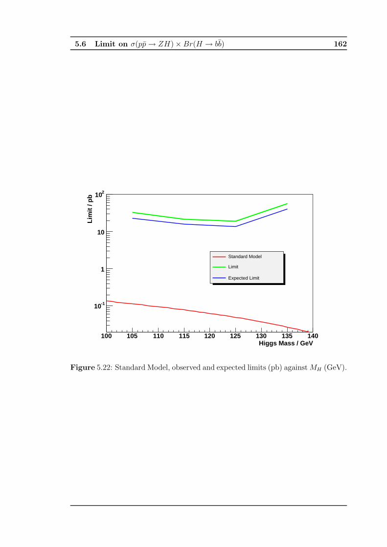
5.6 Limit on σ(pp→ ZH) × Br(H → bb) 162
Higgs Mass / GeV100 105 110 115 120 125 130 135 140
Lim
it /
pb
-110
1
10
210
Standard Model
Limit
Expected Limit
Figure 5.22: Standard Model, observed and expected limits (pb) againstMH (GeV).
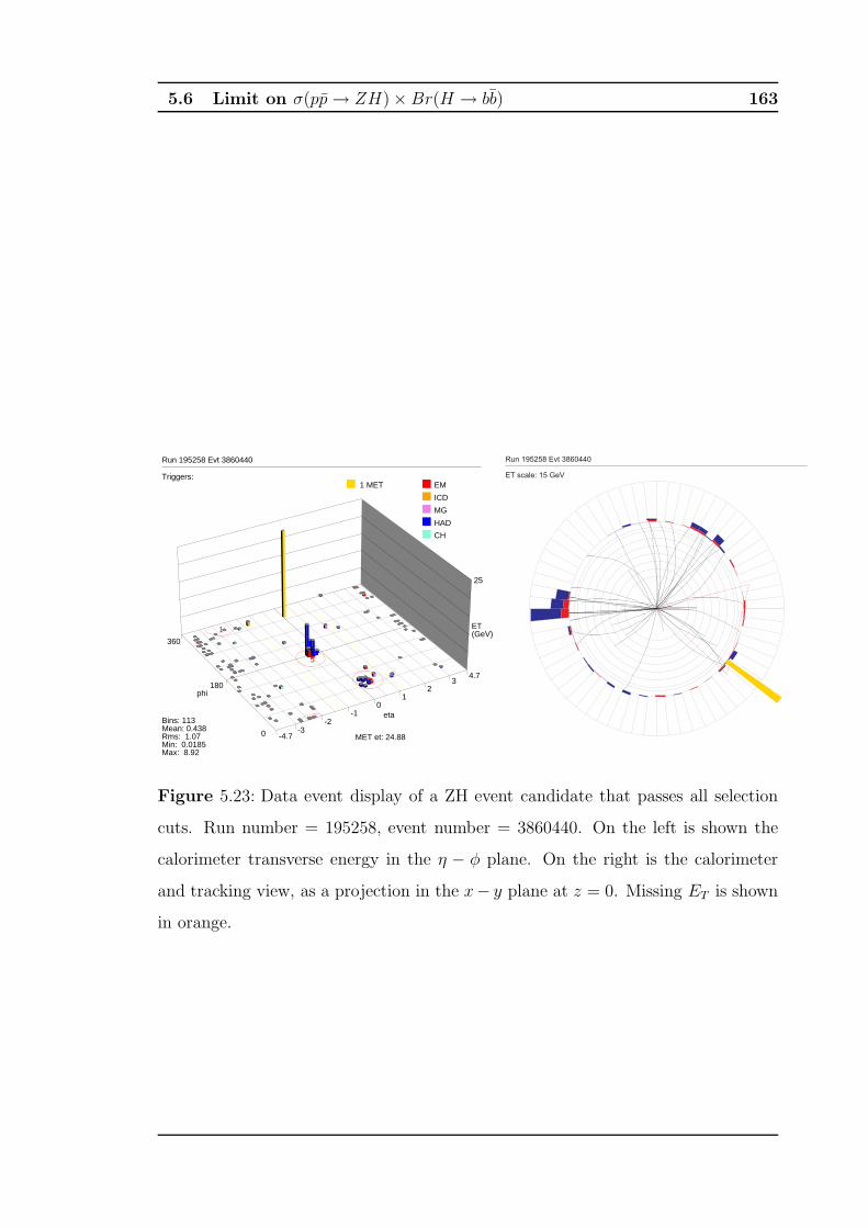
5.6 Limit on σ(pp→ ZH) × Br(H → bb) 163
eta
-4.7 -3
-2 -1
0 1
2 3
4.7
phi180
0
360
ET(GeV)
25
1
5
7
EM
ICD
MG
HAD
CH
1 MET
Bins: 113Mean: 0.438Rms: 1.07Min: 0.0185Max: 8.92
MET et: 24.88
Triggers:
Run 195258 Evt 3860440
ET scale: 15 GeV
Run 195258 Evt 3860440
Figure 5.23: Data event display of a ZH event candidate that passes all selection
cuts. Run number = 195258, event number = 3860440. On the left is shown the
calorimeter transverse energy in the η − φ plane. On the right is the calorimeter
and tracking view, as a projection in the x− y plane at z = 0. Missing ET is shown
in orange.
5.7 Conclusions 164
5.7 Conclusions
A search for ZH → ννbb events on 55.25pb−1 of data, collected with the v13 trigger
list, was carried out. The analysis follows that developed for the v12 trigger list
data sample (261pb−1) in [90]. Improvements in the offline analysis include a Monte
Carlo optimisation of the analysis selection criteria and the first use at DØ of the
neural net (NN) b-tagger tool. In MC, four different light Higgs masses (105GeV,
115GeV, 125GeV and 135GeV) and the main backgrounds listed in Tables 5.2 and
5.3 were simulated. The observed 95% C.L. limits are calculated at between 19.3pb
and 57.1pb; the expected limit is set between 13.8pb and 40.3pb. While these limits
are approximately 2 to 4 times greater than those set in the v12 analysis, they are
comparable with them and with those set in other analyses, given the relatively
small integrated luminosity. The limits set would scale to approximately 10pb for
MH = 115GeV for a 261pb−1 data set. Other recent expected limit results from DØ
include 6.6pb for WH production (174pb−1) [106] and a limit of 9.7pb was set for
ZH production in the µµbb channel[107] (320pb−1). Comparable results from CDF
include 95% C.L. upper limits of 17.8pb to 22.8pb (mH=110GeV to 130 GeV) on
the SM Higgs production cross-section for ZH/WH production, for the H→bb, and
Z→ νν or W→ lν decay channels [108]. Also, an upper limit on the WH production
cross section times branching ratio was set at 3.9pb to 1.3pb. This search used
data corresponding to an integrated luminosity of 955pb−1 and a neural network
b-tagging selection to select double-tagged W+2jet events [109].
This v13 analysis and the v12 analysis are comparable but the improvements in
sensitivity through the MC optimisation and the use of the neural net b-tagger in
this analysis are compensated for by the use of single b-tagged events in addition to
double b-tagged events in the v12 analysis. The use of the neural net b-tagger has
improved the sensitivity of this study, over that of the v12 analysis, by approximately
30% when used instead of the JLIP b-tagger. The MC optimisation of the b-tagging
selection criteria and certain basic selection criteria improves the sensitivity by a
further 15%. The main backgrounds are from the Wjj samples, with the greatest
5.7 Conclusions 165
contributions coming from the events where the W decays to µν. Further work
includes investigating the poor efficiency of the isolated lepton cut further as this
only has an efficiency of approximately 30%, and including the single b-tagged events
in the MC optimisation.
This first look at available v13 data highlights many issues which will need to
be taken into account in the p17 version of the analysis, although data and Monte
Carlo are in reasonable agreement. It is anticipated that the new electromagnetic
and hadronic calorimeter calibration in p17 will have a significant effect on the E/T
distributions and some of these conclusions will have to be revised. From the jet
multiplicity plot in Figure 5.21, it can be seen that there is either a large trigger bias
in the v13 triggers or that there is some problem with the trigger simulation. The
small integrated luminosity of this sample means that the limit set in this analysis
adds little to a combined v12/v13 analysis. So given the imminent availability of p17
data it was deemed worthwhile to spend more time understanding similar factors
in the p17 data, rather than investing further effort understanding the remaining
issues for the p14 v13 data. However as the p14 v12 data, which uses a different
approach to the trigger modelling in Monte Carlo, matches better, it is reasonable
to assume that the discrepancies seen can be traced to the use of d0trigsim to model
the effect of the v13 triggers. The approach taken in this analysis underlies the
p17 analysis and is therefore good preparation in advance of using a larger dataset,
and has demonstrated the potential of the MC optimisation and the neural net
b-tagger for increasing the sensitivity of the ZH → ννbb channel. DØ is moving
towards using more advanced multivariate analysis techniques, such as neural nets,
to make the most of the data by powerfully discriminating against the background
processes. The SUSY Higgs workshop [6] group noted the potential for a neural net
analysis of this channel and this analysis, when carried out on p17 data, will form
a good standard analysis with which to assess such a technique. There are further
improvements in the b-tagging from L0 in the silicon tracker. The new hadronic
calorimeter calibration and TrackCal should improve dijet mass resolution by about
20%.
6 Conclusions 166
Chapter 6
Conclusions
One of the major goals for DØ and the Tevatron is the observation or the ex-
clusion of the Higgs boson. Although the Standard Model, which is based on a
SU(3)⊗SU(2)L⊗U(1)Y symmetry, currently well-describes the strong, electromag-
netic and weak forces and the observed particles, it does not explain the particle
masses that we observe. The Higgs mechanism breaks the symmetry, thus gener-
ating the particle masses and the Higgs boson, but it does not predict the mass
values themselves. Combined results from indirect and direct searches compellingly
indicate that the Higgs has a mass between 114.4GeV and 200GeV. Since the Higgs
is massive, it is only high-energy facilities like the Tevatron, or LHC when it comes
online in 2007, that will be able to discover the Higgs if it exists in this form.
Both the Tevatron and the DØ experiment are running well and exceeding design
expectations. Since DØ came online in 1992, it has undergone extensive upgrades
to improve the detector, compensate for aging parts and to make the most of new
physics opportunities that have arisen with the Tevatron upgrades, most noticeable
the centre of mass energy increase from 1.8TeV to 1.96TeV. The running of the
detector is split into two main runs, Run I and Run II, which is further subdivided
into Run IIa, the focus of this thesis, and Run IIb. The total Run IIa integrated
luminosity, from 19th April 2002 to 23 May 2006, as seen by DØ was 1.18fb−1 ,
operating for much of Run IIa at over 85% efficiency.
6 Conclusions 167
The studies described in this thesis represent a significant contribution to the
DØ experiment. In pp interactions at 1.96TeV, jet production is the dominant
process and so an accurate understanding of this process and the jet energy scale is
essential. Currently, the jet energy scale represents the biggest source of systematic
uncertainty in measurements such as the top mass. At DØ , the jet energy scale, the
energy calibration for jets in the calorimeter, is derived from (γ + jets) data events
using the missing ET projection fraction method which exploits the conservation of
transverse momentum in the pp collisions. As part of the certification of versions
4.2 and 5.1 of the (γ + jets) official jet energy response, the response was calculated
for data and MC for p14 (Z + jets) events, using the missing ET projection fraction
method. Closure tests on (Z + jets) events, were also performed, contributing to the
release of the jet energy scale. These provided a valid cross-check of the response
before it was implemented as part of the jet energy scale at D��O. The (Z + jets) and
(γ + jets) response agreed well within errors but despite using all the then available
data and MC, the lack of statistics still meant that (Z + jets) events could not be
used to derive the full jet energy correction. However, approximately 1fb−1 data is
now available for use with a new collaboration-wide analysis format; it will then be
possible to derive a response for (Z + jets) events with a precision comparable to
the (γ + jets) response.
The b-quark has its own physics programme at DØ as its mass is low enough
that that b-quarks are produced abundantly but high enough that its lifetime is long
enough for it to be easily differentiated from other jets originating from the lighter
quarks. Furthermore, b-quarks are present in the final states of many decays, most
significantly in the decay of Higgs, and specifically in the pp→ZH → ννbb channel,
studied in this thesis. The identification and jet energy scale correction of b-jets is
thus important to the physics programmes at D��O. Scalar and vector corrections to
b-jet energies were derived for events where a jet originating from a b-quark contains
a muon and a neutrino from the direct or cascade decay of the b-quark. Closure
tests on the semileptonic correction showed significant improvement in resolution
over the basic correction for events with one or two semileptonic decays.
To further improve the energy resolution of the calorimeter for low-momentum
charged particles, the implementation of an energy flow algorithm was considered
6 Conclusions 168
by the experiment. This tracks low-momentum particles through the tracker and
into and through the calorimeter, using the tracker momentum measurement as the
energy measurement when the tracker resolution is better. As one of the necessary
steps towards implementing an eflow algorithm at DØ , an electromagnetic cluster
scale was derived using the momenta of low-energy matched-tracks using J/Ψ →e+e− events. The energy of the clusters was shown to be linearly related to the
track momenta with no discernible offset between the cluster energies and the track
momentum. There were insufficient statistics in either the MC or data samples to
detect any variation in the scale with detector η.
Since no η-dependence could be determined, only a scale factor correction could
be derived as expected. It is likely that, with larger event samples, a non-linearity
in track momentum and a variation with η would be observed, and a more effective
correction could be found. It was decided, in 2004, after this study and others
conducted by the eflow working group, that it was more important to do a full
calibration of the current calorimeter rather than invest further effort straightaway
in a full eflow algorithm.
A search for ZH → ννbb events on 55.25pb−1 of data, collected with the v13
trigger list, was carried out. Improvements in the offline analysis included a Monte
Carlo optimisation of the analysis selection criteria and the first use at DØ of the
neural net (NN) b-tagging tool. Four different light Higgs masses (105GeV, 115GeV,
125GeV and 135GeV) and the main backgrounds were simulated. The observed 95%
C.L. limits are calculated at between 19.3pb and 57.1pb; the expected limit is set
between 13.8pb and 40.3pb. While these limits are approximately 2 to 4 times
greater than those set in the previous v12 analysis, they are comparable with them
and with those set in other analyses, given the relatively small integrated luminosity.
This v13 analysis and the v12 analysis are comparable but the improvements in
sensitivity through the MC optimisation and the use of the neural net b-tagger in
this analysis were compensated for by the use of single b-tagged events in addition
to double b-tagged events in the v12 analysis. The use of the neural net b-tagger
improved the sensitivity of this study, over that of the v12 analysis, by approximately
30% when used instead of the JLIP b-tagger. The MC optimisation of the selection
criteria improved the sensitivity by a further 15%. By comparing the jet multiplicity

6.1 Further work and the future 169
of the v13 data with the p14 v12 data, it was apparent that discrepancies arose due
to problems with the use of the DØ trigger simulation.
6.1 Further work and the future
Considering the future of Higgs searches, success will depend critically on three
issues: event yields because the Higgs production cross-sections are small but the
backgrounds large, the efficient identification of b-quarks from Higgs decays and the
invariant Mass peak of Higgs decay products as the sensitivity depends critically on
mass resolution. As the available dataset continues to grow, it will be possible to
make continuous improvements to the jet and semileptonic jet energy scales, improv-
ing mass resolution, and refinements to this search for the Higgs boson. Although a
scalar, muonic semileptonic correction was implemented in JES versions 4.2, 5.1 and
5.3 (p13 and p14 data), there is no semileptonic correction currently available. One
will be implemented soon for our enlarged dataset, also with a vector correction may
be considered and a correction for electronic semileptonic decays. It was decided,
after this study and others conducted by the energy flow working group, that a new,
full calibration of the current calorimeter was the priority and the eflow algorithm
as I worked on it was discontinued. Rather, a basic version of the eflow algorithm,
TrackCal, has now been implemented. The new hadronic calorimeter calibration
and TrackCal will both improve dijet mass resolution by about 20% according to
initial studies. It has been found, following the Higgs Sensitivity study that, as an
approximate rule, an improvement of ±1% in the dijet mass resolution will result
in approximately ∓10% improvement in sensitivity [110].
This first look at available v13 data highlighted many issues which will need
to be taken into account in the p17 version of the analysis, although data and
Monte Carlo are in reasonable agreement. The small data sample meant that the
limit set in this analysis adds little to a combined v12/v13 analysis. So given the
imminent availability of p17 data, studies are being carried out to understand similar
factors in the p17 data, rather than investing further effort in the data set used
in this analysis. The approach taken in this analysis underlies the p17 analysis
and is therefore good preparation in advance of using the larger dataset, and has
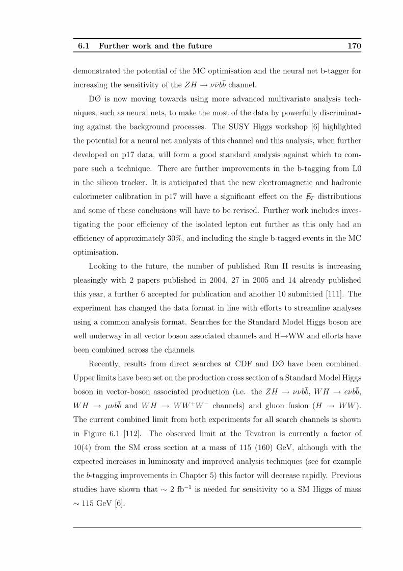
6.1 Further work and the future 170
demonstrated the potential of the MC optimisation and the neural net b-tagger for
increasing the sensitivity of the ZH → ννbb channel.
DØ is now moving towards using more advanced multivariate analysis tech-
niques, such as neural nets, to make the most of the data by powerfully discriminat-
ing against the background processes. The SUSY Higgs workshop [6] highlighted
the potential for a neural net analysis of this channel and this analysis, when further
developed on p17 data, will form a good standard analysis against which to com-
pare such a technique. There are further improvements in the b-tagging from L0
in the silicon tracker. It is anticipated that the new electromagnetic and hadronic
calorimeter calibration in p17 will have a significant effect on the E/T distributions
and some of these conclusions will have to be revised. Further work includes inves-
tigating the poor efficiency of the isolated lepton cut further as this only had an
efficiency of approximately 30%, and including the single b-tagged events in the MC
optimisation.
Looking to the future, the number of published Run II results is increasing
pleasingly with 2 papers published in 2004, 27 in 2005 and 14 already published
this year, a further 6 accepted for publication and another 10 submitted [111]. The
experiment has changed the data format in line with efforts to streamline analyses
using a common analysis format. Searches for the Standard Model Higgs boson are
well underway in all vector boson associated channels and H→WW and efforts have
been combined across the channels.
Recently, results from direct searches at CDF and DØ have been combined.
Upper limits have been set on the production cross section of a Standard Model Higgs
boson in vector-boson associated production (i.e. the ZH → ννbb, WH → eνbb,
WH → µνbb and WH → WW+W− channels) and gluon fusion (H → WW ).
The current combined limit from both experiments for all search channels is shown
in Figure 6.1 [112]. The observed limit at the Tevatron is currently a factor of
10(4) from the SM cross section at a mass of 115 (160) GeV, although with the
expected increases in luminosity and improved analysis techniques (see for example
the b-tagging improvements in Chapter 5) this factor will decrease rapidly. Previous
studies have shown that ∼ 2 fb−1 is needed for sensitivity to a SM Higgs of mass
∼ 115 GeV [6].
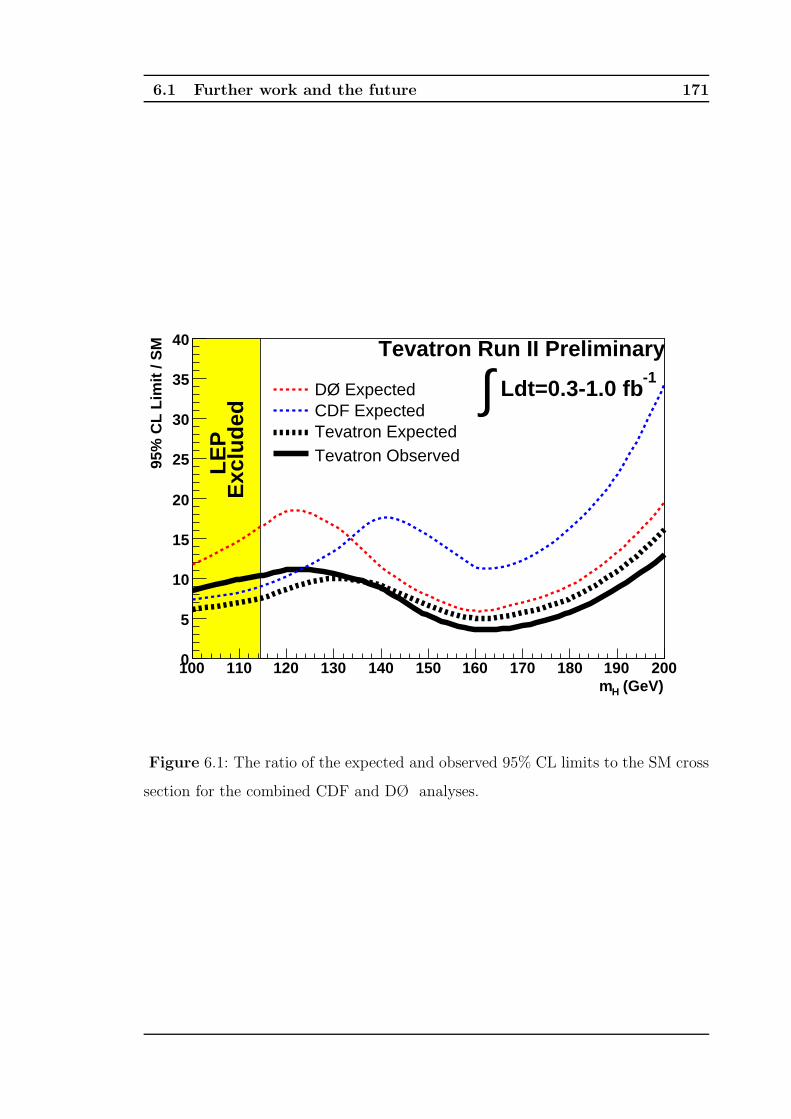
6.1 Further work and the future 171
(GeV)Hm100 110 120 130 140 150 160 170 180 190 200
95%
CL
Lim
it /
SM
0
5
10
15
20
25
30
35
40
DØ ExpectedCDF ExpectedTevatron ExpectedTevatron Observed
Tevatron Run II Preliminary-1
Ldt=0.3-1.0 fb∫
LE
PE
xclu
ded
Figure 6.1: The ratio of the expected and observed 95% CL limits to the SM cross
section for the combined CDF and DØ analyses.
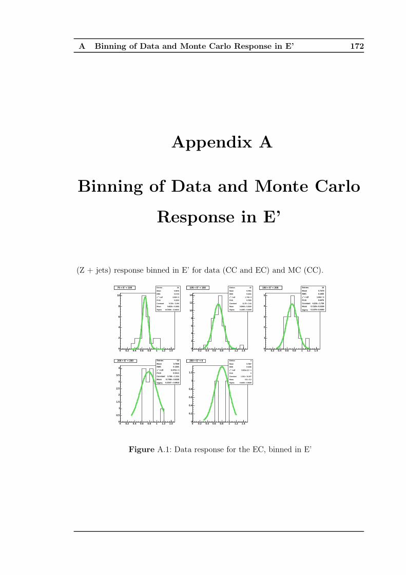
A Binning of Data and Monte Carlo Response in E’ 172
Appendix A
Binning of Data and Monte Carlo
Response in E’
(Z + jets) response binned in E’ for data (CC and EC) and MC (CC).
0 0.2 0.4 0.6 0.8 1 1.2 1.40
2
4
6
8
10
75 < E’ < 105 Entries 26
Mean 0.6976
RMS 0.1713
/ ndf 2χ 6.964 / 5
Prob 0.2233
Constant 3.194± 9.726
Mean 0.0295± 0.6826
Sigma 0.01833± 0.07808
75 < E’ < 105
0 0.2 0.4 0.6 0.8 1 1.2 1.40
2
4
6
8
10
12
14
105 < E’ < 150 Entries 43
Mean 0.7051
RMS 0.1541
/ ndf 2χ 1.745 / 4
Prob 0.7825
Constant 2.41± 11.76
Mean 0.0159± 0.6969
Sigma 0.0199± 0.1385
105 < E’ < 150
0 0.2 0.4 0.6 0.8 1 1.2 1.40
1
2
3
4
5
150 < E’ < 200 Entries 16
Mean 0.7479
RMS 0.1655
/ ndf 2χ 1.652 / 3
Prob 0.6476
Constant 1.739± 4.216
Mean 0.0299± 0.7329
Sigma 0.0680± 0.1479
150 < E’ < 200
0 0.2 0.4 0.6 0.8 1 1.2 1.40
0.5
1
1.5
2
2.5
3
3.5
4
200 < E’ < 250 Entries 12
Mean 0.7939
RMS 0.1366
/ ndf 2χ 0.3731 / 1
Prob 0.5413
Constant 1.215± 3.758
Mean 0.0230± 0.7789
Sigma 0.0912± 0.2347
200 < E’ < 250
0 0.2 0.4 0.6 0.8 1 1.2 1.40
0.2
0.4
0.6
0.8
1
1.2
250 < E’ < 0 Entries 2
Mean 0.7987
RMS 0.1046
/ ndf 2χ 3.933e-12 / -1
Prob 0
Constant 15.107± 1.351
Mean 0.0± 0.8
Sigma 0.8429± 0.1935
250 < E’ < 0
Figure A.1: Data response for the EC, binned in E’
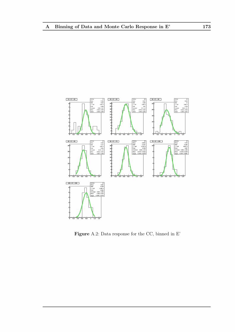
A Binning of Data and Monte Carlo Response in E’ 173
0 0.2 0.4 0.6 0.8 1 1.2 1.40
1
2
3
4
5
6
7
8
12 < E’ < 20 Entries 34
Mean 0.7488
RMS 0.2814
/ ndf 2χ 5.497 / 5
Prob 0.3583
Constant 2.147± 6.351
Mean 0.0250± 0.7626
Sigma 0.0364± 0.1356
12 < E’ < 20
0 0.2 0.4 0.6 0.8 1 1.2 1.40
2
4
6
8
10
12
14
16
18
20
22
20 < E’ < 30 Entries 108
Mean 0.6817
RMS 0.2086
/ ndf 2χ 2.686 / 6
Prob 0.847
Constant 3.0± 21.7
Mean 0.0263± 0.6745
Sigma 0.0204± 0.1849
20 < E’ < 30
0 0.2 0.4 0.6 0.8 1 1.2 1.40
5
10
15
20
25
30 < E’ < 40 Entries 99
Mean 0.6336
RMS 0.2
/ ndf 2χ 3.683 / 6
Prob 0.7195
Constant 2.72± 19.85
Mean 0.0386± 0.6136
Sigma 0.0207± 0.1909
30 < E’ < 40
0 0.2 0.4 0.6 0.8 1 1.2 1.40
5
10
15
20
25
40 < E’ < 55 Entries 83
Mean 0.6566
RMS 0.1471
/ ndf 2χ 4.051 / 5
Prob 0.5421
Constant 3.46± 21.38
Mean 0.0154± 0.6523
Sigma 0.0186± 0.1487
40 < E’ < 55
0 0.2 0.4 0.6 0.8 1 1.2 1.40
2
4
6
8
10
12
14
16
18
20
55 < E’ < 75 Entries 66
Mean 0.6805
RMS 0.1337
/ ndf 2χ 2.719 / 5
Prob 0.7432
Constant 3.40± 18.85
Mean 0.0151± 0.6773
Sigma 0.0179± 0.1343
55 < E’ < 75
0 0.2 0.4 0.6 0.8 1 1.2 1.40
2
4
6
8
10
75 < E’ < 105 Entries 34
Mean 0.739
RMS 0.1455
/ ndf 2χ 2.087 / 5
Prob 0.837
Constant 2.428± 9.485
Mean 0.0290± 0.7379
Sigma 0.0257± 0.1347
75 < E’ < 105
0 0.2 0.4 0.6 0.8 1 1.2 1.40
1
2
3
4
5
6
105 < E’ < 150 Entries 19
Mean 0.806
RMS 0.1262
/ ndf 2χ 1.459 / 2
Prob 0.4821
Constant 1.686± 4.942
Mean 0.033± 0.786
Sigma 0.0742± 0.1688
105 < E’ < 150
Figure A.2: Data response for the CC, binned in E’
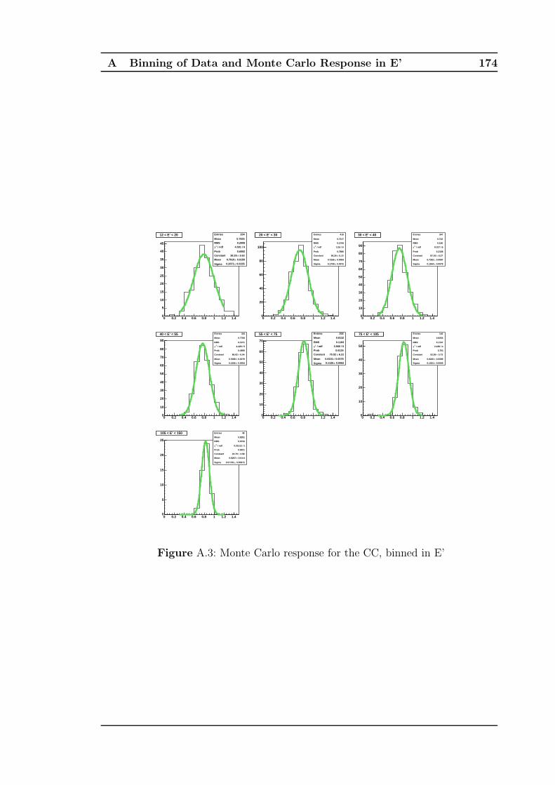
A Binning of Data and Monte Carlo Response in E’ 174
0 0.2 0.4 0.6 0.8 1 1.2 1.40
5
10
15
20
25
30
35
40
45
12 < E’ < 20 Entries 204
Mean 0.7925
RMS 0.2099
/ ndf 2χ 4.501 / 6
Prob 0.6092
Constant 3.63± 38.29
Mean 0.0150± 0.7919
Sigma 0.0155± 0.2071
12 < E’ < 20
0 0.2 0.4 0.6 0.8 1 1.2 1.40
20
40
60
80
100
20 < E’ < 30 Entries 419
Mean 0.7317
RMS 0.1744
/ ndf 2χ 3.16 / 6
Prob 0.7886
Constant 6.10± 96.26
Mean 0.0084± 0.7266
Sigma 0.0072± 0.1708
20 < E’ < 30
0 0.2 0.4 0.6 0.8 1 1.2 1.40
10
20
30
40
50
60
70
80
90
30 < E’ < 40 Entries 347
Mean 0.742
RMS 0.156
/ ndf 2χ 8.317 / 6
Prob 0.2158
Constant 6.37± 87.03
Mean 0.0087± 0.7352
Sigma 0.0078± 0.1544
30 < E’ < 40
0 0.2 0.4 0.6 0.8 1 1.2 1.40
10
20
30
40
50
60
70
80
90
40 < E’ < 55 Entries 301
Mean 0.7708
RMS 0.1371
/ ndf 2χ 4.429 / 5
Prob 0.4895
Constant 6.04± 86.62
Mean 0.0079± 0.7688
Sigma 0.0054± 0.1366
40 < E’ < 55
0 0.2 0.4 0.6 0.8 1 1.2 1.40
10
20
30
40
50
60
70
55 < E’ < 75 Entries 202
Mean 0.8132
RMS 0.1183
/ ndf 2χ 3.566 / 5
Prob 0.6134
Constant 6.31± 70.02
Mean 0.0078± 0.8101
Sigma 0.0062± 0.1125
55 < E’ < 75
0 0.2 0.4 0.6 0.8 1 1.2 1.40
10
20
30
40
50
75 < E’ < 105 Entries 140
Mean 0.8255
RMS 0.1157
/ ndf 2χ 2.189 / 4
Prob 0.701
Constant 5.73± 52.96
Mean 0.0089± 0.8245
Sigma 0.0069± 0.1031
75 < E’ < 105
0 0.2 0.4 0.6 0.8 1 1.2 1.40
5
10
15
20
25
105 < E’ < 150 Entries 48
Mean 0.8281
RMS 0.0733
/ ndf 2χ 0.01512 / 1
Prob 0.9021
Constant 4.58± 24.79
Mean 0.0111± 0.8267
Sigma 0.00973± 0.07795
105 < E’ < 150
Figure A.3: Monte Carlo response for the CC, binned in E’

B Analysis cutflow tables 175
Appendix B
Analysis cutflow tables
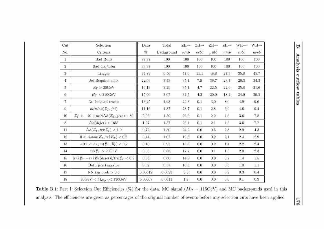
BA
naly
siscutfl
ow
table
s176
Cut Selection Data Total ZH→ ZH→ ZH→ ZH→ WH→ WH→No. Criteria % Background ννbb eebb µµbb τ τ bb eνbb µνbb
1 Bad Runs 99.97 100 100 100 100 100 100 100
2 Bad Cal/Lbn 99.97 100 100 100 100 100 100 100
3 Trigger 34.89 6.56 47.0 11.1 48.8 27.9 35.8 45.7
4 Jet Requirements 22.09 3.43 35.1 7.9 36.7 23.7 26.3 34.3
5 E/T > 20GeV 16.13 3.29 35.1 4.7 22.5 22.6 25.8 31.6
6 HT < 210GeV 15.00 3.07 32.5 4.2 20.0 18.2 24.0 29.5
7 No Isolated tracks 13.25 1.93 29.3 0.1 3.0 8.0 4.9 9.6
9 min△φ(E/T , jet) 11.16 1.87 28.7 0.1 2.8 6.9 4.6 9.4
10 E/T > −40 × min∆φ(E/T , jets) + 80 2.06 1.59 26.6 0.1 2.2 4.6 3.6 7.8
8 △φ(dijet) < 165o 1.97 1.57 26.4 0.1 2.1 4.5 3.6 7.7
11 △φ(E/T , trkE/T ) < 1.0 0.72 1.30 24.2 0.0 0.5 2.8 2.9 4.3
12 0 < Asym(E/T , trkE/T ) < 0.6 0.44 1.07 19.6 0.0 0.2 2.1 2.4 2.9
13 −0.1 < Asym(E/T , H/T ) < 0.2 0.10 0.97 18.8 0.0 0.2 1.4 2.2 2.4
14 trkE/T > 20GeV 0.05 0.88 17.7 0.0 0.1 1.3 2.0 2.3
15 |trkE/T − trkE/T (dijet)|/trkE/T < 0.2 0.03 0.66 14.9 0.0 0.0 0.7 1.4 1.5
16 Both jets taggable 0.02 0.37 10.3 0.0 0.0 0.5 1.0 1.1
17 NN tag prob > 0.5 0.00012 0.0033 3.3 0.0 0.0 0.2 0.3 0.4
18 80GeV < Mdijet < 130GeV 0.00007 0.0011 1.8 0.0 0.0 0.0 0.1 0.2
Table B.1: Part I: Selection Cut Efficiencies (%) for the data, MC signal (MH = 115GeV) and MC backgrounds used in this
analysis. The efficiencies are given as percentages of the original number of events before any selection cuts have been applied
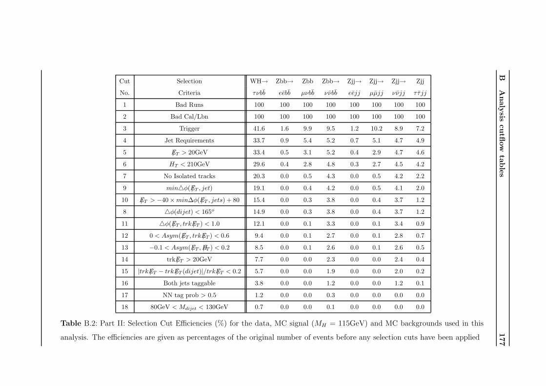
BA
naly
siscutfl
ow
table
s177
Cut Selection WH→ Zbb→ Zbb Zbb→ Zjj→ Zjj→ Zjj→ Zjj
No. Criteria τνbb eebb µνbb ννbb eejj µµjj ννjj τ τ jj
1 Bad Runs 100 100 100 100 100 100 100 100
2 Bad Cal/Lbn 100 100 100 100 100 100 100 100
3 Trigger 41.6 1.6 9.9 9.5 1.2 10.2 8.9 7.2
4 Jet Requirements 33.7 0.9 5.4 5.2 0.7 5.1 4.7 4.9
5 E/T > 20GeV 33.4 0.5 3.1 5.2 0.4 2.9 4.7 4.6
6 HT < 210GeV 29.6 0.4 2.8 4.8 0.3 2.7 4.5 4.2
7 No Isolated tracks 20.3 0.0 0.5 4.3 0.0 0.5 4.2 2.2
9 min△φ(E/T , jet) 19.1 0.0 0.4 4.2 0.0 0.5 4.1 2.0
10 E/T > −40 × min∆φ(E/T , jets) + 80 15.4 0.0 0.3 3.8 0.0 0.4 3.7 1.2
8 △φ(dijet) < 165o 14.9 0.0 0.3 3.8 0.0 0.4 3.7 1.2
11 △φ(E/T , trkE/T ) < 1.0 12.1 0.0 0.1 3.3 0.0 0.1 3.4 0.9
12 0 < Asym(E/T , trkE/T ) < 0.6 9.4 0.0 0.1 2.7 0.0 0.1 2.8 0.7
13 −0.1 < Asym(E/T , H/T ) < 0.2 8.5 0.0 0.1 2.6 0.0 0.1 2.6 0.5
14 trkE/T > 20GeV 7.7 0.0 0.0 2.3 0.0 0.0 2.4 0.4
15 |trkE/T − trkE/T (dijet)|/trkE/T < 0.2 5.7 0.0 0.0 1.9 0.0 0.0 2.0 0.2
16 Both jets taggable 3.8 0.0 0.0 1.2 0.0 0.0 1.2 0.1
17 NN tag prob > 0.5 1.2 0.0 0.0 0.3 0.0 0.0 0.0 0.0
18 80GeV < Mdijet < 130GeV 0.7 0.0 0.0 0.1 0.0 0.0 0.0 0.0
Table B.2: Part II: Selection Cut Efficiencies (%) for the data, MC signal (MH = 115GeV) and MC backgrounds used in this
analysis. The efficiencies are given as percentages of the original number of events before any selection cuts have been applied
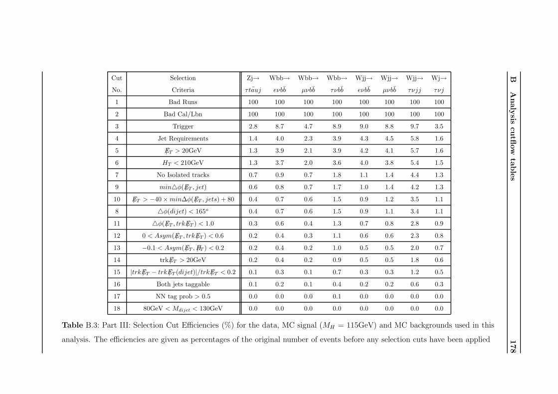
BA
naly
siscutfl
ow
table
s178
Cut Selection Zj→ Wbb→ Wbb→ Wbb→ Wjj→ Wjj→ Wjj→ Wj→No. Criteria τ ¯tauj eνbb µνbb τνbb eνbb µνbb τνjj τνj
1 Bad Runs 100 100 100 100 100 100 100 100
2 Bad Cal/Lbn 100 100 100 100 100 100 100 100
3 Trigger 2.8 8.7 4.7 8.9 9.0 8.8 9.7 3.5
4 Jet Requirements 1.4 4.0 2.3 3.9 4.3 4.5 5.8 1.6
5 E/T > 20GeV 1.3 3.9 2.1 3.9 4.2 4.1 5.7 1.6
6 HT < 210GeV 1.3 3.7 2.0 3.6 4.0 3.8 5.4 1.5
7 No Isolated tracks 0.7 0.9 0.7 1.8 1.1 1.4 4.4 1.3
9 min△φ(E/T , jet) 0.6 0.8 0.7 1.7 1.0 1.4 4.2 1.3
10 E/T > −40 × min∆φ(E/T , jets) + 80 0.4 0.7 0.6 1.5 0.9 1.2 3.5 1.1
8 △φ(dijet) < 165o 0.4 0.7 0.6 1.5 0.9 1.1 3.4 1.1
11 △φ(E/T , trkE/T ) < 1.0 0.3 0.6 0.4 1.3 0.7 0.8 2.8 0.9
12 0 < Asym(E/T , trkE/T ) < 0.6 0.2 0.4 0.3 1.1 0.6 0.6 2.3 0.8
13 −0.1 < Asym(E/T , H/T ) < 0.2 0.2 0.4 0.2 1.0 0.5 0.5 2.0 0.7
14 trkE/T > 20GeV 0.2 0.4 0.2 0.9 0.5 0.5 1.8 0.6
15 |trkE/T − trkE/T (dijet)|/trkE/T < 0.2 0.1 0.3 0.1 0.7 0.3 0.3 1.2 0.5
16 Both jets taggable 0.1 0.2 0.1 0.4 0.2 0.2 0.6 0.3
17 NN tag prob > 0.5 0.0 0.0 0.0 0.1 0.0 0.0 0.0 0.0
18 80GeV < Mdijet < 130GeV 0.0 0.0 0.0 0.0 0.0 0.0 0.0 0.0
Table B.3: Part III: Selection Cut Efficiencies (%) for the data, MC signal (MH = 115GeV) and MC backgrounds used in this
analysis. The efficiencies are given as percentages of the original number of events before any selection cuts have been applied
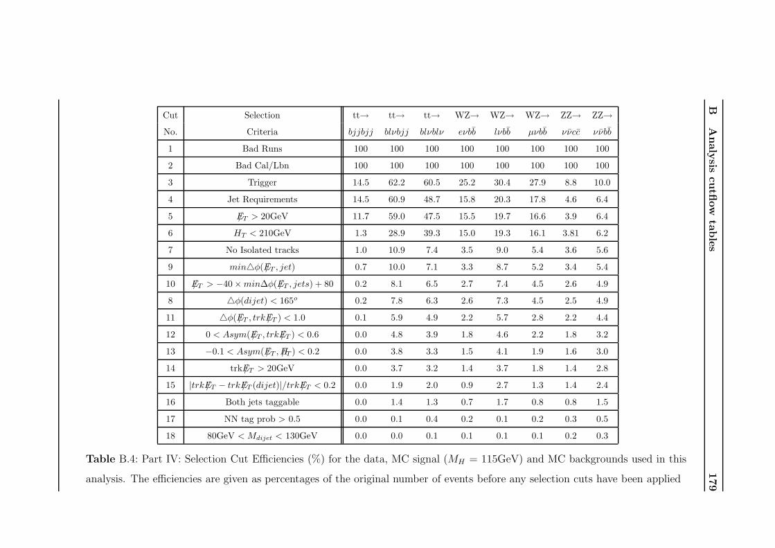
BA
naly
siscutfl
ow
table
s179
Cut Selection tt→ tt→ tt→ WZ→ WZ→ WZ→ ZZ→ ZZ→No. Criteria bjjbjj blνbjj blνblν eνbb lνbb µνbb ννcc ννbb
1 Bad Runs 100 100 100 100 100 100 100 100
2 Bad Cal/Lbn 100 100 100 100 100 100 100 100
3 Trigger 14.5 62.2 60.5 25.2 30.4 27.9 8.8 10.0
4 Jet Requirements 14.5 60.9 48.7 15.8 20.3 17.8 4.6 6.4
5 E/T > 20GeV 11.7 59.0 47.5 15.5 19.7 16.6 3.9 6.4
6 HT < 210GeV 1.3 28.9 39.3 15.0 19.3 16.1 3.81 6.2
7 No Isolated tracks 1.0 10.9 7.4 3.5 9.0 5.4 3.6 5.6
9 min△φ(E/T , jet) 0.7 10.0 7.1 3.3 8.7 5.2 3.4 5.4
10 E/T > −40 × min∆φ(E/T , jets) + 80 0.2 8.1 6.5 2.7 7.4 4.5 2.6 4.9
8 △φ(dijet) < 165o 0.2 7.8 6.3 2.6 7.3 4.5 2.5 4.9
11 △φ(E/T , trkE/T ) < 1.0 0.1 5.9 4.9 2.2 5.7 2.8 2.2 4.4
12 0 < Asym(E/T , trkE/T ) < 0.6 0.0 4.8 3.9 1.8 4.6 2.2 1.8 3.2
13 −0.1 < Asym(E/T , H/T ) < 0.2 0.0 3.8 3.3 1.5 4.1 1.9 1.6 3.0
14 trkE/T > 20GeV 0.0 3.7 3.2 1.4 3.7 1.8 1.4 2.8
15 |trkE/T − trkE/T (dijet)|/trkE/T < 0.2 0.0 1.9 2.0 0.9 2.7 1.3 1.4 2.4
16 Both jets taggable 0.0 1.4 1.3 0.7 1.7 0.8 0.8 1.5
17 NN tag prob > 0.5 0.0 0.1 0.4 0.2 0.1 0.2 0.3 0.5
18 80GeV < Mdijet < 130GeV 0.0 0.0 0.1 0.1 0.1 0.1 0.2 0.3
Table B.4: Part IV: Selection Cut Efficiencies (%) for the data, MC signal (MH = 115GeV) and MC backgrounds used in this
analysis. The efficiencies are given as percentages of the original number of events before any selection cuts have been applied
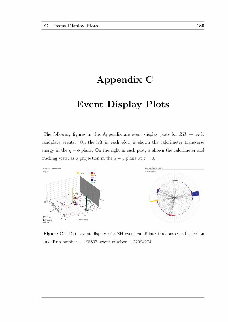
C Event Display Plots 180
Appendix C
Event Display Plots
The following figures in this Appendix are event display plots for ZH → ννbb
candidate events. On the left in each plot, is shown the calorimeter transverse
energy in the η − φ plane. On the right in each plot, is shown the calorimeter and
tracking view, as a projection in the x− y plane at z = 0.
eta
-4.7 -3
-2 -1
0 1
2 3
4.7
phi180
0
360
ET(GeV)
40
1 0
27
11 44
31
14
15
EM
ICD
MG
HAD
CH
1 MET
Bins: 271Mean: 0.682Rms: 2.91Min: 0.00949Max: 35
MET et: 37.95
Triggers:
Run 195837 Evt 22994974
ET scale: 41 GeV
Run 195837 Evt 22994974
Figure C.1: Data event display of a ZH event candidate that passes all selection
cuts. Run number = 195837, event number = 22994974
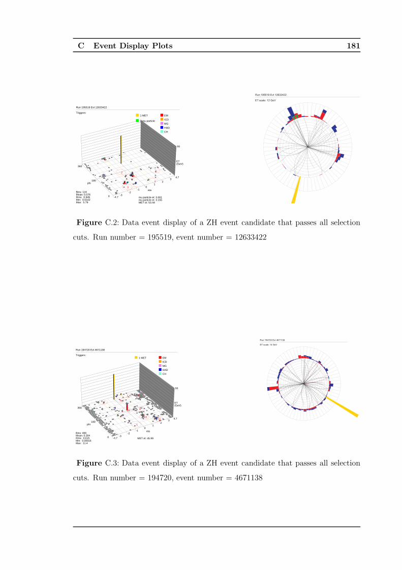
C Event Display Plots 181
eta
-4.7 -3
-2 -1
0 1
2 3
4.7
phi180
0
360
ET(GeV)
55
7
228
2
3
2
EM
ICD
MG
HAD
CH
1 MET
2 mu particle
Bins: 124Mean: 0.576Rms: 0.949Min: 0.0102Max: 5.79
mu particle et: 3.001mu particle et: 3.155MET et: 53.44
Triggers:
Run 195519 Evt 12633422
ET scale: 12 GeV
Run 195519 Evt 12633422
Figure C.2: Data event display of a ZH event candidate that passes all selection
cuts. Run number = 195519, event number = 12633422
eta
-4.7 -3
-2 -1
0 1
2 3
4.7
phi180
0
360
ET(GeV)
50
2
2
3
6
28 6
18
1
11
EM
ICD
MG
HAD
CH
1 MET
Bins: 466Mean: 0.264Rms: 0.615Min: 0.00916Max: 11.4
MET et: 45.99
Triggers:
Run 194720 Evt 4671138
ET scale: 14 GeV
Run 194720 Evt 4671138
Figure C.3: Data event display of a ZH event candidate that passes all selection
cuts. Run number = 194720, event number = 4671138
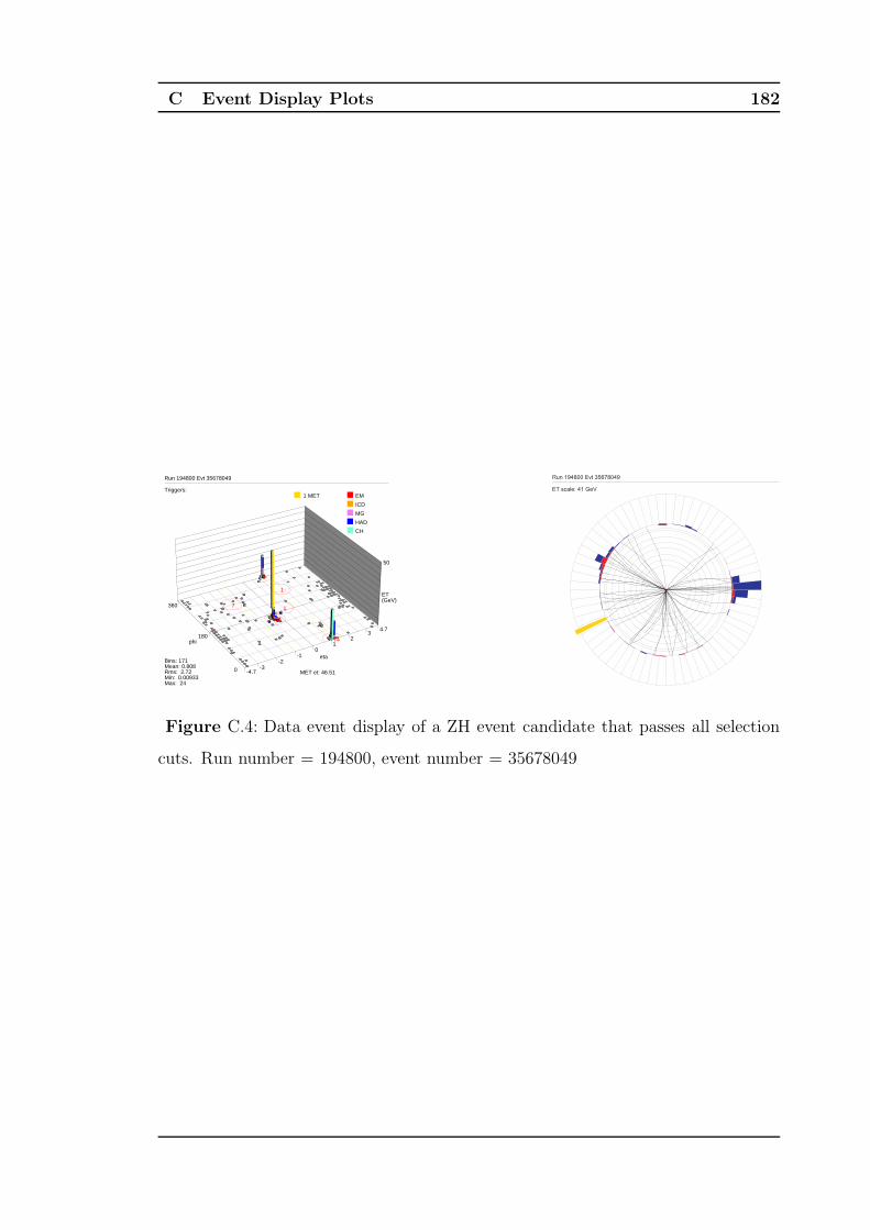
C Event Display Plots 182
eta
-4.7 -3
-2 -1
0 1
2 3
4.7
phi180
0
360
ET(GeV)
50
1
7 1
41
74
EM
ICD
MG
HAD
CH
1 MET
Bins: 171Mean: 0.808Rms: 2.72Min: 0.00933Max: 24
MET et: 46.51
Triggers:
Run 194800 Evt 35678049
ET scale: 41 GeV
Run 194800 Evt 35678049
Figure C.4: Data event display of a ZH event candidate that passes all selection
cuts. Run number = 194800, event number = 35678049
BIBLIOGRAPHYBIBLIOGRAPHY 183
Bibliography
[1] I.Brock. The Higgs Potential. http://www-zeus.physik.uni-bonn.de/
~brock/feynman/vtp_ws0506/chapter09/higgs_pot.jpg.
[2] K. Riesselmann. Limitations of a Standard Model Higgs Boson. hep-
ph/9711456, 1997.
[3] ALEPH Collaboration, DELPHI Collaboration, L3 Collaboration and OPAL
Collaboration, The SLD Collaboration, The LEP Electroweak Working Group,
The SLD Electroweak and Heavy Flavour Groups. Precision electroweak mea-
surements on the Z Resonance. hep-ex/0509008, 2006.
[4] The DØ Collaboration. Run II Luminosity. http://www-d0.fnal.gov/
runcoor/RUN/run2_lumi.html.
[5] A. Goussiou et al. Jet Energy Scale and Resolution, v4.2. DØ Note 4115,
2003.
[6] The CDF and DØ Collaborations. Results of the Tevatron Higgs Sensitivity
Study. FERMILAB-PUB-03/320-E, 2003.
[7] M. Spira. Higgs Boson Production and Decay at the Tevatron. hep-
ph/9810289, 1998.
[8] W. M. Yao et al. The Review of Particle Physics. Journal of Physics, G 33,
1, 2006.
[9] A. Askew. Parametrising the Local Muon Resolution in p13. DØ note 4314,
2003.
BIBLIOGRAPHYBIBLIOGRAPHY 184
[10] T. Scanlon and M. Anastasoaie et al. Development and Optimisation on
Monte Carlo of a Neural Network Tool to Identify b-jets. DØ note 4889, 4889.
[11] Particle Data Group. A History of Particle Physics. http:
//particleadventure.org/particleadventure/other/history/index.
html.
[12] D. Griffiths. Introduction to Elementary Particles. John Wiley and Sons,
Inc., 1987.
[13] F. Halzen and A. Martin. Quarks and Leptons: An Introductory Course in
Modern Particle Physics. John Wiley and Sons, Inc., 1984.
[14] Emmy Noether. Preface. Mathematischer Annalen, 96:26–11, 1927.
[15] C. Yang and R. Mills. Conservation of Isotopic Spin and Isotopic Gauge
Invariance. Phys. Rev., 96(1):191–195, Oct 1954.
[16] S. Glashow. Partial Symmetries of Weak Interactions. Nucl. Phys., 22:579–
588, 1961.
[17] A. Salam. Weak and Electromagnetic Interactions. Svartholm: Elementary
Particle Theory, Proceedings of the Nobel Symposium 1968, 1968.
[18] S. Weinberg. A Model of Leptons. Phys. Rev. Lett., 19(21):1264–1266, Nov
1967.
[19] The Super Kamiokande Collaboration. Evidence for the Oscillation of Atmo-
spheric Neutrinos. Phys. Rev. Lett. 81, pages 1562–1567, 1998.
[20] The Super Kamiokande Collaboration. Determination of Solar Neutrino Os-
cillation Parameters using 1496 Days of Super Kamiokande I Data. Phys. Lett.
B539, pages 179–187, 2002.
[21] N. Arkani-Hamed et al. The Hierarchy Problem and Dew Dimensions at a
Millimeter Scale. Phys. Lett., B429:263–272, 1998.
BIBLIOGRAPHYBIBLIOGRAPHY 185
[22] P. Higgs. Broken Symmetries and the Masses of Gauge Bosons. Phys. Rev.
Lett., 13(16):508–509, Oct 1964.
[23] P. Higgs. Spontaneous Symmetry Breakdown without Massless Bosons. Phys.
Rev., 145(4):1156–1163, May 1966.
[24] C. Lai. Gauge Theory of Weak and Electromagnetic Interactions. Selected
Papers. World Scientfic, 1981.
[25] B. Lee et al. Weak Interactions at Very High Energies: The Role of the Higgs
Boson Bass. Phys. Rev. D, 16(5):1519–1531, Sep 1977.
[26] ALEPH Collaboration, DELPHI Collaboration, L3 Collaboration, OPAL Col-
laboration. Search for the Standard Model Higgs Boson at LEP. Physics
Letters B, 565:61, 2003.
[27] M. Kruse et al. Combined Standard Model VH Production Cross Section
Limits for Run I CDF. CDF Note 4985, 1999.
[28] The DØ Collaboration. Description of Original DØ Detector. Nucl Instrum.
Methods Phys. Res. A, pages 338–185, 1994.
[29] The DØ Collaboration. Observation of the Top Quark. Phys. Rev. Lett.,
74(14):2632–2637, Apr 1995.
[30] The DØ Collaboration. Direct Measurement of the Top Quark Mass. Phys.
Rev. Lett., 79(7):1197–1202, Aug 1997.
[31] The DØ Collaboration. A Precision Measurement of the Mass of the Top
Quark. Nature, 429:638–642, Jun 2004.
[32] The DØ Collaboration. The Upgraded DØ Detector. Nucl.Instrum.Meth.,
A565:463–537, 2006.
[33] The DØ Collaboration. Run IIb Upgrade Technical Design Re-
port. http: // d0server1. fnal. gov/ projects/ run2b/ Silicon/ www/
smt2b/ Documentation/ documentation. html , September 2002.
BIBLIOGRAPHYBIBLIOGRAPHY 186
[34] T. Cole et al. Design Report, Superconducting Accelerator. Technical Report
Beams-doc-1888-v1, Fermilab, 1979.
[35] R. Moore. An Overview of Tevatron Collider Run II at Fermilab. Technical
Report Beams-doc-190-v1, Fermilab, Dec 2002.
[36] X. Hailey. Production of Negative Hydrogen Ions. http://sist.fnal.gov/
archive/2003/Hailey/Paper.pdf.
[37] Wikipedia. Stochastic cooling. http://en.wikipedia.org/wiki/
Stochastic_cooling, 2006.
[38] D. Adams et al. First Large Sample Study of Visible Light Photon Counters
(VLPC’s). http://d0server1.fnal.gov/users/stefan/www/como94/como.
html.
[39] The DØ Collaboration. Beam Tests of the DØ Uranium Liquid Argon End
Calorimeters. DØ Note 1434, 1992.
[40] The DØ Collaboration. The Muon System of the Run II DØ Detector. Nuclear
Instruments and Methods in Physics Research A, 552 (2005) 372-398, 2005.
[41] Definitions. http://www.fnal.gov/pub/now/definitions/.
[42] T. Edwards et al. Determination of the Effective Inelastic pp Cross-section
for the DØ Run II Luminosity Measurement. Fermilab-TM-2278-E, 2004.
[43] T. Andeen et al. The Upgraded Luminosity Detector Readout and Studies of
the New Effective Inelastic Cross-section. DØ Note 4904, 2005.
[44] S. Klimenko et al. Averaging of the Inelastic Cross-sections Measured by the
CDF and the E811 Experiments. Fermilab, 2004. FERMILAB-FN-0741.
[45] B. Casey et al. Determination of the Effective Inelastic pp Cross-section for
the DØ Luminosity Measurement Using Upgraded Readout Electronics. DØ
Note 4958, 2005.

BIBLIOGRAPHYBIBLIOGRAPHY 187
[46] G. Steinbruck. Measurement of the Angular Distribution of Electrons from
W Boson Decays at DØ . PhD thesis, University of Oklahoma, 1999.
[47] V. Buescher and J. Zhu. EM Certification Tools. DØ Note 4171, 2003.
[48] The DØ Collaboration. Top Quark Search with the DØ 1992 to 1993 Data
Sample. Phys. Rev. D, 52(9):4877–4919, Nov 1995.
[49] The EM ID Working Group. DØ EM ID Certification. http://www-d0.
fnal.gov/phys_id/emid/d0_private/certification/main_v5_0.html.
[50] J. Gardner et al. Electron Likelihood in p14. DØ Note 4449, 2004.
[51] C. Clement et al. Muon ID Certification for p14. DØ Note 4350, 2004.
[52] E. Busato and B. Andrieu. Jet Algorithms in the DØ Run II Software:
Description and User’s Guide. DØ Note 4457, 2004.
[53] G. Blazey et al. Run II Jet Physics. Proc. of the QCD and Weak Boson
Physics in Run II Workshop, 1999.
[54] N. Hadley. Cone Algorithm for Jet Finding. DØ Note 0904, 1989.
[55] The Top Physics Working Group of the DØ Collaboration. DØ Top Analysis
and Data Sample for the Winter Conference 2004. DØ Note 4419, 2004.
[56] B. Olivier et al. The Missing Transverse Energy Resolution of an Event. DØ
Note 3629, 1999.
[57] The DØ Tracking Working Group. Tracking Efficiency Overview. Technical
report, DØ Collaboration, 2006.
[58] H. Greenlee. Motion of a Charged Particle in a Magnetic Field. DØ Note
4180, 2003.
[59] D. Adams. Finding Tracks. DØ Note 2958-2, 1996.
[60] G. Hesketh. Central Track Extrapolation through the DØ Detector. DØ Note
4079, 2003.

BIBLIOGRAPHYBIBLIOGRAPHY 188
[61] G. Borissov. Technical Details of AA Tracking. Talk presented at the DØ
Workshop, December 2005.
[62] The Tracking Working Group. Performance of p14 Tracking. http://www-d0.
fnal.gov/global_tracking/results/p14.00.00_index.html.
[63] The B-ID Working Group. Secondary Vertex Tagger. http:
//www-d0.fnal.gov/phys_id/bid/d0_private/certification/p14/
secvertex/secvertex_v2.html.
[64] L. Feligioni et al. Update on b-quark Jet Identification with Secondary Vertex
Reconstruction using d0reco p14. DØ Note 4414, 2004.
[65] The DØ Collaboration. Run II Software Algorithms. http://www-d0.fnal.
gov/computing/algorithms/.
[66] The Common Samples Group. d0correct. http://www-d0.fnal.gov/
Run2Physics/cs/d0correct/d0correct.html.
[67] S. Protopopescu et al. ThumbNail: a Compact Data Format. DØ Note 3979,
2002.
[68] The DØ Collaboration. Trigger webpages. http://www-d0.fnal.gov/
detector/trigger.html.
[69] The DØ Top Physics Working Group. Public results. http://www-d0.fnal.
gov/Run2Physics/top/top_public_web_pages/top_public.html.
[70] The Jet Energy Scale Working Group. Certified Jet Energy
Scale. http://www-d0.fnal.gov/phys_id/jes/d0_private/certified/
certified_jes.html.
[71] B. Abbott et al. Determination of the Absolute Jet Energy Scale in the DØ
Calorimeters. hep-ex/9805009, 1998.
[72] The Jet Energy Scale Working Group. The Jetcorr Software Package. http:
//www-d0.fnal.gov/d0dist/dist/packages/jetcorr/.
BIBLIOGRAPHYBIBLIOGRAPHY 189
[73] The DØ Collaboration. Run II Reconstruction Status. http://www-d0.fnal.
gov/computing/algorithms/status/p14.html.
[74] T. Sjstrand et al. PYTHIA 6.3 Physics and Manual. hep-ph/0308153, 2003.
[75] The Electromagnetic Object Identification Working Group. EM Identification.
http://www-d0.fnal.gov/phys_id/emid/d0_private/emid.html.
[76] The Jet Identification Working Group. Jet Identification. http://www-d0.
fnal.gov/phys_id/jets/jetid.html.
[77] L. Duflot and M. Ridel. An Energy Flow Algorithm for DØ . DØ Note 3927,
2002.
[78] M. Petteni et al. Energy Correction for Semileptonic Decays of b-jets, using
p13. DØ Note 4248, 2003.
[79] K. Hanagaki and J. Kasper. Identification of b-jet by Soft Muon Tagging.
DØ Note 4867, 2005.
[80] The ALEPH Collaboration. Performance of the ALEPH detector at LEP.
Nuclear Instruments and Methods in Physics, A360(3):481–506, June 1995.
[81] L. Dulfot and M. Ridel. The CellNN Algorithm: Cell Level Clustering in the
DØ Calorimeter. DØ Note 3923, 2001.
[82] F. Beaudette and J.-F. Grivaz. The Road Method (an Algorithm for the
Identification of Electrons in Jets). DØ Note 3976, April 11, 2002.
[83] F. Beaudette and J.-F. Grivaz. Electron Identification and b-tagging with
the Road Method. DØ Note 4032, October 3, 2002.
[84] The Electromagnetic Object Identification Working Group. EMRECO: EM
ID Vertical Review.
[85] The Electromagnetic Object Identification Working Group. EM Particle Doc-
umentation.

BIBLIOGRAPHYBIBLIOGRAPHY 190
[86] M. Cwiok and A. Haas. Run II η-Intercalibration of the Hadronic Calorimeter.
DØ Note 5006, 2006.
[87] J. Kvita and K.Peters. Run II φ-Intercalibration of the Fine Hadronic
Calorimeter. DØ Note 5005, 2006.
[88] P. Mal. Energy Flow Status: Single Pion Response, Track-Calorimeter Jets.
DØ Calorimeter Workshop, April 2006.
[89] M. Carena et al. Report of the Tevatron Higgs Working Group. hep-
ph/0010338, 2000.
[90] M. Tomoto. A Search for SM Higgs Boson using the zh → ννbb Channel in
pp Collisions at√
(s) = 1.96TeV. DØ Note 4744, 2005.
[91] The Common Samples Working Group. p14 Data Reprocessing Pages. http:
//www-d0.fnal.gov/Run2Physics/cs/skimming/pass2.html.
[92] The Common Samples Working Group. Thumbnail Fixing. http://www-d0.
fnal.gov/Run2Physics/cs/fixing/fixing.html.
[93] M. Mangano et al. Alpgen, a generator for hard multiparton processes in
hadronic collisions. hep-ph/0206293, 2003.
[94] J. Campbell and R. Ellis. MCFM: A Monte Carlo for Femtobarn processes
at Hadron Colliders. http://mcfm.fnal.gov.
[95] A. Duperrin et al. The v13 Physics Trigger List and New Phenomena Triggers.
DØ Note 4641, 2004.
[96] The DØ Collaboration. Certified Jet Energy Scale v5.3. http://www-d0.
fnal.gov/phys_id/jes/d0_private/certified/v5.3/links.html.
[97] C. Gerber et al. Taggability in p14 Pass 2 Data. DØ Note 4995, 2006.
[98] T. Scanlon et al. Certification of the Neural Network b-tagging Tool on Pass
2 Data. DØ Note 4890, 2005.

BIBLIOGRAPHYBIBLIOGRAPHY 191
[99] D. Bloch et al. Performance of the JLIP b-tagger in p14. DØ Note 4348,
2004.
[100] B-ID Certification Group. DØ Secondary Vertex Tag Certification.
http://www-d0.fnal.gov/phys_id/bid/d0_private/certification/p14/
secvertex/secvertex_v1.html.
[101] B-ID Certification Group. The Counting Signed Impact Paramter
Tagging Method. http://www-d0.fnal.gov/phys_id/bid/d0_private/
certification/p14/CSIP/CSIP_v2.html.
[102] F. James. MINUIT, Function Minimization and Error Analysis, Reference
Manual. CERN Program Library Long Writeup D506, Version 94.1, 2000.
[103] M. Agelou et al. 0.5 and 0.7 Jet pT Resolution using JES v5.3. DØ Note
4775, 2005.
[104] I. Bertram et al. A Recipe for the Construction of Confidence Limits. DØ
Note 2775, 1995.
[105] J. Hobbs. Bayesian Limit Calculator Web Interface. http://www-d0.fnal.
gov/hobbs/limitcalc.html.
[106] The DØ Collaboration. A Search for wbb and wh Production in pp Collisions
at√
s = 1.96TeV. hep-ex/0410062, 2004.
[107] H. Dong and J. Hobbs. Search for SM Higgs Boson in zh → µµbb Channel
pp Collisions at√
s = 1.96TeV. DØ Note 5107, 2006.
[108] V. Veszpremi et al. Search for the SM Higgs Boson in the E/T +b-jets Final
State with 0.973fb−1 Run II data at CDF. CDF Note CDF8442, 2006.
[109] Y. Kusakabe et al. Search for Standard Model Higgs Boson Production in
Association with W Boson at CDF with 1fb−1. CDF Note CDF8390, 2006.
[110] Wade Fisher, On behalf of the Tevatron Higgs Sensitivity Group. Tevatron
higgs sensitivity. Conference Proceedings, 2004.

BIBLIOGRAPHYBIBLIOGRAPHY 192
[111] The DØ Collaboration. DØ Run II Publications. http://www-d0.fnal.gov/
www_buffer/pub/Run2_publications.html.
[112] G. Bernardi et al. Limits on Standard Model Higgs Boson Production. DØ
Note 5056, 2006.

“The traveller has reached the end of the journey!”
The Dhammapada, Buddha