· J. DifferentialEquations 250 (2011) 340–366 Contents lists available at ScienceDirect JournalofDifferentialEquations Homographicsolutionsofthecurved3

J. Differential Equations 250 (2011) 340–366

Contents lists available at ScienceDirect

Journal of Differential Equations

www.elsevier.com/locate/jde

Homographic solutions of the curved 3-body problem

Florin Diacu a,∗, Ernesto Pérez-Chavela b

a Pacific Institute for the Mathematical Sciences and Department of Mathematics and Statistics, University of Victoria, P.O. Box 3060 STNCSC, Victoria, BC, Canada, V8W 3R4b Departamento de Matemáticas, Universidad Autónoma Metropolitana-Iztapalapa, Apdo. 55534, México, D.F., Mexico

a r t i c l e i n f o a b s t r a c t

Article history:Received 22 January 2010Revised 13 August 2010

In the 2-dimensional curved 3-body problem, we prove the exis-tence of Lagrangian and Eulerian homographic orbits, and providetheir complete classification in the case of equal masses. We alsoshow that the only non-homothetic hyperbolic Eulerian solutionsare the hyperbolic Eulerian relative equilibria, a result that provestheir instability.

© 2010 Elsevier Inc. All rights reserved.

1. Introduction

We consider the 3-body problem in spaces of constant curvature (κ �= 0), which we will call thecurved 3-body problem, to distinguish it from its classical Euclidean (κ = 0) analogue. The potential(defined by the force function Uκ in (4), below) generalizes the Newtonian potential and preservesits basic properties: it is a harmonic function and generates a central field for which bounded orbitsare closed.

This research direction started in the 1830s, when Janos Bolyai and Nikolai Lobachevsky proposeda curved 2-body problem, which was broadly studied by several mathematicians, including ErnestSchering [22,23], Wilhem Killing [12–14], and Heinrich Liebmann [17,18]. Many of the results obtainedby these authors, as well as new ones, were recently proved with the help of modern methods byJosé Cariñena, Manuel Rañada, and Mariano Santander [1]. The study of the quantum analogue ofthe curved 2-body problem was proposed by Erwin Schrödinger [24], Leopold Infeld [10], and AlfredSchild [11]. Other attempts at extending the Newtonian case to spaces of constant curvature, such asthe one of Rudolph Lipschitz [19], did not survive, mostly because the proposed potentials lacked thebasic properties mentioned above.

The newest results occur in [3], a paper in which we obtained a unified framework that providesthe equations of motion of the curved n-body problem for any n � 2 and κ �= 0. We also proved there

* Corresponding author.E-mail addresses: [email protected] (F. Diacu), [email protected] (E. Pérez-Chavela).

0022-0396/$ – see front matter © 2010 Elsevier Inc. All rights reserved.doi:10.1016/j.jde.2010.08.011

http://dx.doi.org/10.1016/j.jde.2010.08.011

http://www.ScienceDirect.com/

http://www.elsevier.com/locate/jde

mailto:[email protected]

mailto:[email protected]

http://dx.doi.org/10.1016/j.jde.2010.08.011

F. Diacu, E. Pérez-Chavela / J. Differential Equations 250 (2011) 340–366 341

the existence of several classes of relative equilibria, including the Lagrangian orbits mentioned above.Relative equilibria are orbits for which the configuration of the system remains congruent with itselffor all time, i.e. the distances between any two bodies are constant during the motion.

The study of the curved n-body problem, for n � 3, might help us understand the nature of thephysical space. Gauss allegedly tried to determine the nature of space by measuring the angles of atriangle formed by the peaks of three mountains. Even if the goal of his topographic measurementswas different from what anecdotical history attributes to him (see [20]), this method of deciding thenature of space remains valid for astronomical distances. But since we cannot measure the anglesof cosmic triangles, we could alternatively check whether specific (potentially observable) motions ofcelestial bodies occur in spaces of negative, zero, or positive curvature, respectively.

We showed in [3] that while Lagrangian orbits (rotating equilateral triangles having the bodiesat their vertices) of non-equal masses are known to occur for κ = 0, they must have equal massesfor κ �= 0. Since Lagrangian solutions of non-equal masses exist in our solar system (for example,the triangle formed by the Sun, Jupiter, and the Trojan asteroids), we can conclude that, if assumedto have constant curvature, the physical space is Euclidean for distances of the order 101 AU. Thediscovery of new orbits of the curved 3-body problem, as defined here in the spirit of an old tradition,might help us extend our understanding of space to larger scales.

So far, the only other existing paper on the curved n-body problem, treated in a unified context,deals with singularities [4], a subject we will not approach here. But relative equilibria can be put ina broader perspective. They are also the object of Saari’s conjecture (see [21,5]), which we partiallysolved for the curved n-body problem [3]. Saari’s conjecture has recently generated a lot of interestin classical celestial mechanics (see the references in [5,6]) and is still unsolved for n > 3. Moreover,it led to the formulation of Saari’s homographic conjecture [21,6], a problem that is directly relatedto the purpose of this research.

We study here certain solutions that are more general than relative equilibria, namely orbits forwhich the configuration of the system remains similar with itself. In this class of solutions, the relativedistances between particles may change proportionally during the motion, i.e. the size of the systemmay vary, though its shape remains the same. We will call these solutions homographic, in agreementwith the classical terminology [25].

In the classical Newtonian case [25], as well as in more general classical contexts [2], the standardconcept for understanding homographic solutions is that of central configuration. This notion, how-ever, seems to have no meaningful analogue in spaces of constant curvature because it implies theexistence of the first integrals of the centre of mass, which are absent in the curved case. The inte-grals of the centre of mass and linear momentum seem to be specific only to Euclidean space. Indeed,n-body problems derived by discretizing Einstein’s field equations, as obtained by Tullio Levi-Civita[15,16], as well as Albert Einstein, Leopold Infeld, and Banesh Hoffmann [8], also lack such integrals.

We focus here on three types of homographic solutions. The first, which we call Lagrangian, forman equilateral triangle at every time instant. We ask that the plane of this triangle be always orthog-onal to the rotation axis. This assumption seems to be natural because, as proved in [3], Lagrangianrelative equilibria, which are particular homographic Lagrangian orbits, obey this property, and rela-tive equilibria that lack this property fail to exist. We prove the existence of homographic Lagrangianorbits in Section 3, and provide their complete classification in the case of equal masses in Section 4,for κ > 0, and Section 5, for κ < 0. Moreover, we show in Section 6 that Lagrangian solutions withnon-equal masses don’t exist.

We then study another type of homographic solutions of the curved 3-body problem, which wecall Eulerian, in analogy with the classical case that refers to bodies confined to a rotating straightline. At every time instant, the bodies of an Eulerian homographic orbit are on a (possibly) rotatinggeodesic. In Section 7 we prove the existence of these orbits. Moreover, for equal masses, we providetheir complete classification in Section 8, for κ > 0, and Section 9, for κ < 0.

Finally, in Section 10, we discuss the existence of hyperbolic homographic solutions, which occuronly for negative curvature. We prove that when the bodies are on the same hyperbolically rotatinggeodesic, a class of solutions we call hyperbolic Eulerian, every orbit is a hyperbolic Eulerian relativeequilibrium. Therefore hyperbolic Eulerian relative equilibria are unstable, a fact which makes themunlikely observable candidates in a (hypothetical) hyperbolic physical universe.

342 F. Diacu, E. Pérez-Chavela / J. Differential Equations 250 (2011) 340–366

2. Equations of motion

We consider the equations of motion on 2-dimensional manifolds of constant curvature, namelyspheres embedded in R

3, for κ > 0, and hyperboloids1 embedded in the Minkovski space M3, for

κ < 0.Consider the masses m1,m2,m3 > 0 in R

3, for κ > 0, and in M3, for κ < 0, whose positions are

given by the vectors qi = (xi, yi, zi), i = 1,2,3. Let q = (q1,q2,q3) be the configuration of the system,and p = (p1,p2,p3), with pi = mi qi , representing the momentum. We define the gradient operatorwith respect to the vector qi as

∇qi = (∂xi , ∂yi ,σ ∂zi ),

where σ is the signature function,

σ ={+1, for κ > 0,

−1, for κ < 0,(1)

and let ∇ denote the operator (∇q1 , ∇q2 , ∇q3 ). For the 3-dimensional vectors a = (ax,ay,az) and b =(bx,by,bz), we define the inner product

a � b := (axbx + ayby + σazbz) (2)

and the cross product

a ⊗ b := (aybz − azby,azbx − axbz,σ (axby − aybx)

). (3)

The Hamiltonian function of the system describing the motion of the 3-body problem in spaces ofconstant curvature is

Hκ (q,p) = Tκ (q,p) − Uκ (q),

where

Tκ (q,p) = 1

2

3∑i=1

m−1i (pi � pi)(κqi � qi)

defines the kinetic energy and

Uκ (q) =∑

1�i< j�3

mim j|κ |1/2κqi � q j

[σ(κqi � qi)(κq j � q j) − σ(κqi � q j)2]1/2

(4)

is the force function, −Uκ representing the potential energy.2 Then the Hamiltonian form of theequations of motion is given by the system{

qi = m−1i pi,

pi = ∇qi Uκ (q) − m−1i κ(pi � pi)qi, i = 1,2,3, κ �= 0,

(5)

1 The hyperboloid corresponds to Weierstrass’s model of hyperbolic geometry (see the appendix in [3]).2 In [3] we showed how this expression of Uκ follows from the cotangent potential for κ �= 0, and that U0 is the Newtonian

potential of the Euclidean problem, obtained as κ → 0.


where the gradient of the force function has the expression

∇qi Uκ (q) =3∑

j=1j �=i

mim j|κ |3/2(κq j � q j)[(κqi � qi)q j − (κqi � q j)qi][σ(κqi � qi)(κq j � q j) − σ(κqi � q j)

2]3/2. (6)

The motion is confined to the surface of nonzero constant curvature κ , i.e. (q,p) ∈ T∗(M2κ )3, where

T∗(M2κ )3 is the cotangent bundle of the configuration space (M2

κ )3, and

M2κ = {

(x, y, z) ∈ R3∣∣ κ(

x2 + y2 + σ z2) = 1}.

In particular, M21 = S2 is the 2-dimensional sphere, and M2−1 = H2 is the 2-dimensional hyperbolic

plane, represented by the upper sheet of the hyperboloid of two sheets (see the appendix of [3] formore details). We will also denote M2

κ by S2κ for κ > 0, and by H2

κ for κ < 0.Notice that the 3 constraints given by κqi � qi = 1, i = 1,2,3, imply that qi � pi = 0, so the 18-

dimensional system (5) has 6 constraints. The Hamiltonian function provides the integral of energy,

Hκ (q,p) = h,

where h is the energy constant. Eqs. (5) also have the integrals of the angular momentum,

3∑i=1

qi ⊗ pi = c, (7)

where c = (α,β,γ ) is a constant vector. Unlike in the Euclidean case, there are no integrals of thecenter of mass and linear momentum. Their absence complicates the study of the problem since manyof the standard methods don’t apply anymore.

Using the fact that κqi � qi = 1 for i = 1,2,3, we can write system (5) as

qi =3∑

j=1j �=i

m j|κ |3/2[q j − (κqi � q j)qi][σ − σ(κqi � q j)

2]3/2− (κ qi � qi)qi, i = 1,2,3, (8)

which is the form of the equations of motion we will use in this paper. The sums in the right-hand side of the above equations represent the gradient of the potential. When κ → 0, both thesphere (for κ → 0 through positive values) and the hyperboloid (for κ → 0 through negative values)become planes at infinity, relative to the centre of the frame. The segments through the origin ofthe frame whose angle measures the distance between two points on the curved surface becomeparallel and infinite, so the distance in the limit plane is the Euclidean distance. Consequently thepotential tends to the Newtonian potential as κ → 0 (see [3] for more details). The terms involvingthe velocities occur because of the constraints imposed by the curvature. When κ → 0, these termsobviously vanish.

3. Local existence and uniqueness of Lagrangian solutions

In this section we define the Lagrangian solutions of the curved 3-body problem, which forma particular class of homographic orbits. Then, for equal masses and suitable initial conditions, weprove their local existence and uniqueness.

Definition 1. A solution of Eqs. (8) is called Lagrangian if, at every time t , the masses form an equi-lateral triangle that is orthogonal to the z axis.


Though we explained in the Introduction why the orthogonality condition seems to be natural, wewere, so far, unable to prove that, if they don’t obey it, homographic orbits that change size do notexist. We conjecture, however, that this property is true.

According to Definition 1, the size of a Lagrangian solution can vary, but its shape is always thesame. Moreover, all masses have the same coordinate z(t), which may also vary in time, though thetriangle is always perpendicular to the z axis.

We can represent a Lagrangian solution of the curved 3-body problem in the form

q = (q1,q2,q3), with qi = (xi, yi, zi), i = 1,2,3, (9)

x1 = r cosω, y1 = r sinω, z1 = z,

x2 = r cos(ω + 2π/3), y2 = r sin(ω + 2π/3), z2 = z,

x3 = r cos(ω + 4π/3), y3 = r sin(ω + 4π/3), z3 = z,

where z = z(t) satisfies z2 = σκ−1 − σ r2; σ is the signature function defined in (1); r := r(t) is thesize function; and ω := ω(t) is the angular function.

Indeed, for every time t , we have that x2i (t) + y2

i (t) + σ z2i (t) = κ−1, i = 1,2,3, which means that

the bodies stay on the surface M2κ , each body has the same z coordinate, i.e. the plane of the triangle

is orthogonal to the z axis, and the angles between any two bodies, seen from the geometric centerof the triangle, are always the same, so the triangle remains equilateral. Therefore representation (9)of the Lagrangian orbits agrees with Definition 1.

Definition 2. A Lagrangian solution of Eqs. (8) is called Lagrangian homothetic if the equilateral trian-gle expands or contracts, but does not rotate around the z axis.

In terms of representation (9), a Lagrangian solution is Lagrangian homothetic if ω(t) is constant,but r(t) is not constant. Such orbits occur, for instance, when three bodies of equal masses lying ini-tially in the same open hemisphere are released with zero velocities from an equilateral configuration,to end up in a triple collision.

Definition 3. A Lagrangian solution of Eqs. (8) is called a Lagrangian relative equilibrium if the trianglerotates around the z axis without expanding or contracting.

In terms of representation (9), a Lagrangian relative equilibrium occurs when r(t) is constant, butω(t) is not constant. Of course, Lagrangian homothetic solutions and Lagrangian relative equilibria,whose existence we proved in [3], are particular Lagrangian orbits, but we expect that the Lagrangianorbits are not reduced to them. We now show this by proving the local existence and uniqueness ofLagrangian solutions that are neither Lagrangian homothetic, nor Lagrangian relative equilibria.

Theorem 1. In the curved 3-body problem of equal masses, m1 = m2 = m3 := m > 0, for every set of initialconditions belonging to a certain class, the local existence and uniqueness of a Lagrangian solution, which bothrotates and changes size, is assured.

Proof. We will check to see if Eqs. (8) admit solutions of the form (9) that start in the region z > 0and for which both r(t) and ω(t) are not constant. We compute then that

κqi � q j = 1 − 3κr2/2 for i, j = 1,2,3, with i �= j,

x1 = r cosω − rω sinω, y1 = r sinω + rω cosω,

x2 = r cos

(ω + 2π

3

)− rω sin

(ω + 2π

3

),


y2 = r sin

(ω + 2π

3

)+ rω cos

(ω + 2π

3

),

x3 = r cos

(ω + 4π

3

)− rω sin

(ω + 4π

3

),

y3 = r sin

(ω + 4π

3

)+ rω cos

(ω + 4π

3

),

z1 = z2 = z3 = −σ rr(σκ−1 − σ r2)−1/2

, (10)

κ qi � qi = κr2ω2 + κ r2

1 − κr2for i = 1,2,3,

x1 = (r − rω2) cosω − (rω + 2rω) sinω,

y1 = (r − rω2) sinω + (rω + 2rω) cosω,

x2 = (r − rω2) cos

(ω + 2π

3

)− (rω + 2rω) sin

(ω + 2π

3

),

y2 = (r − rω2) sin

(ω + 2π

3

)+ (rω + 2rω) cos

(ω + 2π

3

),

x3 = (r − rω2) cos

(ω + 4π

3

)− (rω + 2rω) sin

(ω + 4π

3

),

y3 = (r − rω2) sin

(ω + 4π

3

)+ (rω + 2rω) cos

(ω + 4π

3

),

z1 = z2 = z3 = −σ rr(σκ−1 − σ r2)−1/2 − κ−1r2(σκ−1 − σ r2)−3/2

.

Substituting these expressions into system (8), we are led to the system below, where the double-dotterms on the left indicate to which differential equation each algebraic equation corresponds:

x1: A cosω − B sinω = 0,

x2: A cos

(ω + 2π

3

)− B sin

(ω + 2π

3

)= 0,

x3: A cos

(ω + 4π

3

)− B sin

(ω + 4π

3

)= 0,

y1: A sinω + B cosω = 0,

y2: A sin

(ω + 2π

3

)+ B cos

(ω + 2π

3

)= 0,

y3: A sin

(ω + 4π

3

)+ B cos

(ω + 4π

3

)= 0,

z1, z2, z3: A = 0,

where

A := A(t) = r − r(1 − κr2)ω2 + κrr2

1 − κr2+ 24m(1 − κr2)

r2(12 − 9κr2)3/2,

B := B(t) = rω + 2rω.


Obviously, the above system has solutions if and only if A = B = 0, which means that the localexistence and uniqueness of Lagrangian orbits with equal masses is equivalent to the existence ofsolutions of the system of differential equations⎧⎪⎪⎪⎪⎨⎪⎪⎪⎪⎩

r = ν,

w = −2νw

r,

ν = r(1 − κr2)w2 − κrν2

1 − κr2− 24m(1 − κr2)

r2(12 − 9κr2)3/2

(11)

with initial conditions r(0) = r0, w(0) = w0, ν(0) = ν0, where w = ω. The functions r, ω, and ware analytic, and as long as the initial conditions satisfy the conditions r0 > 0 for all κ , as wellas r0 < κ−1/2 for κ > 0, standard results of the theory of differential equations guarantee the localexistence and uniqueness of a solution (r, w, ν) of Eqs. (11), and therefore the local existence anduniqueness of a Lagrangian orbit with r(t) and ω(t) not constant. The proof is now complete. �4. Classification of Lagrangian solutions for κ > 0

We can now state and prove the following result:

Theorem 2. In the curved 3-body problem with equal masses, m1 = m2 = m3 := m, and κ > 0 there are fiveclasses of Lagrangian solutions:

(i) Lagrangian homothetic orbits that begin or end in total collision in finite time;(ii) Lagrangian relative equilibria that move on a circle;

(iii) Lagrangian periodic orbits that both rotate and change size;(iv) Lagrangian non-periodic, non-collision orbits that eject at time −∞, with zero velocity, from the equator,

reach a maximum distance from the equator, which depends on the initial conditions, and return to theequator, with zero velocity, at time +∞.

None of the above orbits can cross the equator, defined as the great circle of the sphere orthogonal to the zaxis.

(v) Lagrangian equilibrium points, when the three equal masses are fixed on the equator at the vertices of anequilateral triangle.

The rest of this section is dedicated to the proof of this theorem.Let us start by noticing that the first two equations of system (11) imply that w = − 2rw

r , whichleads to

w = c

r2,

where c is a constant. The case c = 0 can occur only when w = 0, which means ω = 0. Under thesecircumstances the angular velocity is zero, so the motion is homothetic. These are the orbits whoseexistence is stated in Theorem 2(i). They occur only when the angular momentum is zero, and leadto a triple collision in the future or in the past, depending on the sense of the velocity vectors.

For the rest of this section, we assume that c �= 0. Then system (11) takes the form⎧⎨⎩r = ν,

ν = c2(1 − κr2)

3− κrν2

2− 24m(1 − κr2)

2 2 3/2.

(12)

r 1 − κr r (12 − 9κr )


Notice that the term κrν2

1−κr2 of the last equation arises from the derivatives z1, z2, z3 in (10). Butthese derivatives would be zero if the equilateral triangle rotates along the equator, because r is con-stant in this case, so the term κrν2

1−κr2 vanishes. Therefore the existence of equilateral relative equilibriaon the equator (included in statement (ii) above), and the existence of equilibrium points (stated in(v))—results proved in [3]—are in agreement with the above equations. Nevertheless, the term κrν2

1−κr2

stops any orbit from crossing the equator, a fact mentioned before statement (v) of Theorem 2.Understanding system (12) is the key to proving Theorem 2. We start with the following facts:

Lemma 1. Assume κ,m > 0 and c �= 0. Then for κ1/2c2 − (8/√

3)m < 0, system (12) has two fixed points,while for κ1/2c2 − (8/

√3)m � 0 it has one fixed point.

Proof. The fixed points of system (12) are given by r = 0 = ν. Substituting ν = 0 in the secondequation of (12), we obtain

1 − κr2

r2

[c2

r− 24m

(12 − 9κr2)3/2

]= 0.

The above remarks show that, for κ > 0, r = κ−1/2 is a fixed point, which physically represents anequilateral relative equilibrium moving along the equator. Other potential fixed points of system (12)are given by the equation

c2(12 − 9κr2)3/2 = 24mr,

whose solutions are the roots of the polynomial

729c4κ3r6 − 2916c4κ2r4 + 144(27c4κ + 4m2)r2 − 1728. (13)

Writing x = r2 and assuming κ > 0, this polynomial takes the form

p(x) = 729κ3x3 − 2916c4κ2x2 + 144(27c4κ + 4m2)x − 1728, (14)

and its derivative is given by

p′(x) = 2187c4κ3x2 − 5832c4κ2x + 144(27c4κ + 4m2). (15)

The discriminant of p′ is −5038848c4κ3m2 < 0.

By Descartes’s rule of signs, p can have one or three positive roots. If p has three positive roots,then p′ must have two positive roots, but this is not possible because its discriminant is negative.Consequently p has exactly one positive root.

For the point (r, ν) = (r0,0) to be a fixed point of Eqs. (12), r0 must satisfy the inequalities 0 <

r0 � κ−1/2. If we denote

g(r) = c2

r− 24m

(12 − 9κr2)3/2, (16)

we see that, for κ > 0, g is a decreasing function since

dg(r) = −c2

2− 648mκr

2 5/2< 0. (17)

dr r (12 − 9κr )


When r → 0, we obviously have that g(r) > 0 since we assumed c �= 0. When r → κ−1/2, we haveg(r) → κ1/2c2 − (8/

√3)m. If κ1/2c2 − (8/

√3)m > 0, then r0 > κ−1/2, so (r0,0) is not a fixed point.

Therefore, assuming c �= 0, a necessary condition that (r0,0) is a fixed point of system (12) with0 < r0 < κ−1/2 is that

κ1/2c2 − (8/√

3)m < 0.

For κ1/2c2 − (8/√

3)m � 0, the only fixed point of system (12) is (r, ν) = (κ−1/2,0). This conclusioncompletes the proof of the lemma. �4.1. The flow in the (r, ν) plane for κ > 0

We will now study the flow of system (12) in the (r, ν) plane for κ > 0. At every point with ν �= 0,the slope of the vector field is given by dν

dr , i.e. by the ratio νr = h(r, ν), where

h(r, ν) = c2(1 − κr2)

νr3− κrν

1 − κr2− 24m(1 − κr2)

νr2(12 − 9κr2)3/2.

Since h(r,−ν) = −h(r, ν), the flow of system (12) is symmetric with respect to the r axis for r ∈(0, κ−1/2]. Also notice that, except for the fixed point (κ−1/2,0), system (12) is undefined on thelines r = 0 and r = κ−1/2. Therefore the flow of system (12) exists only for points (r, ν) in the band(0, κ−1/2) × R and for the point (κ−1/2,0).

Since r = ν , no interval on the r axis can be an invariant set for system (12). Then the symmetryof the flow relative to the r axis implies that orbits cross the r axis perpendicularly. But since g(r) �= 0at every non-fixed point, the flow crosses the r axis perpendicularly everywhere, except at the fixedpoints.

Let us further treat the case of one fixed point and the case of two fixed points separately.

4.1.1. The case of one fixed pointA single fixed point, namely (κ−1/2,0), appears when κ1/2c2 − (8/

√3)m � 0. Then the function g ,

which is decreasing, has no zeroes for r ∈ (0, κ−1/2), therefore g(r) > 0 in this interval, so the flowalways crosses the r axis upwards.

For ν �= 0, the right-hand side of the second equation of (12) can be written as

G(r, ν) = g1(r)g(r) + g2(r, ν), (18)

where

g1(r) = 1 − κr2

r2and g2(r, ν) = − κrν2

1 − κr2. (19)

But ddr g1(r) = −2/r3 < 0 and ∂

∂r g2(r, ν) = − κν2(1+κr2)

(1−κr2)2 < 0. So, like g , the functions g1 and g2 are

decreasing in (0, κ−1/2), with g1, g > 0, therefore G is a decreasing function as well. Consequently,for ν = constant > 0, the slope of the vector field decreases from +∞ at r = 0 to −∞ at r = κ−1/2.For ν = constant < 0, the slope of the vector field increases from −∞ at r = 0 to +∞ at r = κ−1/2.

This behavior of the vector field forces every orbit to eject downwards from the fixed point, at timet = −∞ and with zero velocity, on a trajectory tangent to the line r = κ−1/2, reach slope zero at somemoment in time, then cross the r axis perpendicularly upwards and symmetrically return with finalzero velocity, at time t = +∞, to the fixed point (see Fig. 1(a)). So the flow of system (12) consists inthis case solely of homoclinic orbits to the fixed point (κ−1/2,0), orbits whose existence is claimedin Theorem 2(iv). Some of these trajectories may come very close to a total collapse, which theywill never reach because only solutions with zero angular momentum (like the homothetic orbits)encounter total collisions, as proved in [4].


Fig. 1. A sketch of the flow of system (12) for (a) κ = c = 1, m = 0.24, typical for one fixed point, and (b) κ = c = 1, m = 4,typical for two fixed points.

So the orbits cannot reach any singularity of the line r = 0, and neither can they begin or endin a singularity of the line r = κ−1/2. The reason for the latter is that such points are of the form(κ−1/2, ν) with ν �= 0, therefore r �= 0 at such points. But the vector field tends to infinity whenapproaching the line r = κ−1/2, so the flow must be tangent to it, consequently r must tend to zero,which is a contradiction. Therefore only homoclinic orbits exist in this case.

4.1.2. The case of two fixed pointsTwo fixed points, (κ−1/2,0) and (r0,0), with 0 < r0 < κ−1/2, occur when κ1/2c2 − (8/

√3)m < 0.

Since g is decreasing in the interval (0, κ−1/2), we can conclude that g(t) > 0 for t ∈ (0, r0) andg(t) < 0 for t ∈ (r0, κ

−1/2). Therefore the flow of system (12) crosses the r axis upwards when r < r0,but downwards for r > r0 (see Fig. 1(b)).

The function G(r, ν), defined in (18), fails to be decreasing in the interval (0, κ−1/2) along lines ofconstant ν , but it has no singularities in this interval and still maintains the properties

limr→0+ G(r, ν) = +∞ and lim

r→(κ−1/2)−G(r, ν) = −∞.

Therefore G must vanish at some point, so due to the symmetry of the vector field with respect tothe r axis, the fixed point (r0,0) is surrounded by periodic orbits. The points where G vanishes aregiven by the nullcline ν = 0, which has the expression

ν2 = (1 − κr2)2

κr3

[c2

r− 24m

(12 − 9κr2)3/2

].

This nullcline is a disconnected set, formed by the fixed point (κ−1/2,0) and a continuous curve,symmetric with respect to the r axis. Indeed, since the equation of the nullcline can be written as

ν2 = (1−κr2)2

κr3 g(r), and limr→(κ−1/2)− g(r) = κ1/2c2 − (8/√

3)m < 0 in the case of two fixed points (as

shown in the proof of Lemma 1), only the point (κ−1/2,0) satisfies the nullcline equation away fromthe fixed point (r0,0).

The asymptotic behavior of G near r = κ−1/2 also forces the flow to produce homoclinic orbitsfor the fixed point (κ−1/2,0), as in the case discussed in Section 4.1.1. The existence of these twokinds of solutions is stated in Theorem 2(iii) and (iv), respectively. The fact that orbits cannot begin


or end at any of the singularities of the lines r = 0 or r = κ−1/2 follows as in Section 4.1.1. This remarkcompletes the proof of Theorem 2.

5. Classification of Lagrangian solutions for κ < 0


Theorem 3. In the curved 3-body problem with equal masses, m1 = m2 = m3 := m, and κ < 0 there are eightclasses of Lagrangian solutions:

(i) Lagrangian homothetic orbits that begin or end in total collision in finite time;(ii) Lagrangian relative equilibria, for which the bodies move on a circle parallel with the xy plane;

(iii) Lagrangian periodic orbits that change size;(iv) Lagrangian orbits that eject at time −∞ from a certain relative equilibrium solution s (whose existence

and position depend on the values of the parameters) and return to it at time +∞;(v) Lagrangian orbits that come from infinity at time −∞ and reach the relative equilibrium s at time +∞;

(vi) Lagrangian orbits that eject from the relative equilibrium s at time −∞ and reach infinity at time +∞;(vii) Lagrangian orbits that come from infinity at time −∞ and symmetrically return to infinity at time +∞,

never able to reach the Lagrangian relative equilibrium s;(viii) Lagrangian orbits that come from infinity at time −∞, reach a position close to a total collision, and

symmetrically return to infinity at time +∞. The minimum size of this orbit is, for given κ , m, and c,smaller than the corresponding orbit described in (ii).

The rest of this section is dedicated to the proof of this theorem. Notice first that the orbits de-scribed in Theorem 3(i) occur for zero angular momentum, when c = 0, as for instance when thethree equal masses are released with zero velocities from the Lagrangian configuration, a case inwhich a total collapse takes place at the point (0,0, |κ |−1/2). Depending on the initial conditions, themotion can be bounded or unbounded. The existence of the orbits described in Theorem 3(ii) wasproved in [3]. To address the other points of Theorem 3, and show that no other orbits than the onesstated there exist, we need to study the flow of system (12) for κ < 0. Let us first prove the followingfact:

Lemma 2. Assume κ < 0, m > 0, and c �= 0. Then system (12) has no fixed points when 27c4κ + 4m2 � 0,and can have two, one, or no fixed points when 27c4κ + 4m2 > 0.

Proof. The number of fixed points of system (12) is the same as the number of positive zeroes of thepolynomial p defined in (14). If 27c4κ + 4m2 � 0, all coefficients of p are negative, so by Descartes’srule of signs, p has no positive roots.

Now assume that 27c4κ + 4m2 > 0. Then the zeroes of p are the same as the zeroes of the monicpolynomial (i.e. with leading coefficient 1):

p(x) = x3 − 4κ−1x2 + [48κ−2 + (64/81)c−4κ−3m2]x − (64/27)κ−3,

obtained when dividing p by the leading coefficient. But a monic cubic polynomial can be written as

x3 − (a1 + a2 + a3)x2 + (a1a2 + a2a3 + a3a1)x − a1a2a3,

where a1, a2, and a3 are its roots. One of these roots is always real and has the opposite sign of−a1a2a3. Since the free term of p is positive, one of its roots is always negative, independently of theallowed values of the coefficients κ , m, c. Consequently p can have two positive roots (including thepossibility of a double positive root) or no positive root at all. Therefore system (12) can have two,one, or no fixed points. As we will see later, all three cases occur. �

We further state and prove a property, which we will use to establish Lemma 4:


Lemma 3. Assume κ < 0,m > 0, c �= 0, let (r∗,0) be a fixed point of system (12), and consider the function g

defined in (16). Then ddr g(r∗) = 0 if and only if r∗ = (− 2

3κ )1/2 . Moreover, d2

dr2 g(r∗) > 0.

Proof. Since (r∗,0) is a fixed point of system (12), it follows that g(r∗) = 0. Then it follows from re-lation (16) that (12 − 9κr2∗)3/2 = 24mr∗/c2. Substituting this value of (12 − 9κr2∗)3/2 into the equationddr g(r∗) = 0, which is equivalent to

648mκr∗(12 − 9κr2∗)5/2

= −c2

r2∗,

it follows that 27κ/(12 − 9κr2∗) = −1/r2∗ . Therefore r∗ = (− 23κ )1/2. Obviously, for this value of r∗ ,

g(r∗) = 0, so the first part of Lemma 3 is proved. To prove the second part, substitute r∗ = (− 23κ )1/2

into the equation g(r∗) = 0, which is then equivalent with the relation

9√

3c2(−κ)1/2 − 4m = 0. (20)

Notice that

d2

dr2g(r) = 2c2

r3− 648mκ

(12 − 9κr2)5/2− 29160mκ2r2

(12 − 9κr2)7/2.

Substituting for r∗ = (− 23κ )1/2 in the above equation, and using (20), we are led to the conclusion

that d2

dr2 g(r∗) = −(2√

3 + 6√

2)mκ/9√

6, which is positive for κ < 0. This completes the proof. �The following result is important for understanding a qualitative aspect of the flow of system (12),

which we will discuss later in this section.

Lemma 4. Assume κ < 0,m > 0, c �= 0, and let (r∗,0) be a fixed point of system (12). If ∂∂r G(r∗,0) = 0, then

∂2

∂r2 G(r∗,0) > 0, where G is defined in (18).

Proof. Since (r∗,0) is a fixed point of (12), G(r∗,0) = 0. But for κ < 0, we have g1(r∗) > 0, so

necessarily g(r∗) = 0. Moreover, ddr g1(r∗) �= 0, and since ∂

∂r g2(r, ν) = − κν2(1+κr2)

(1−κr2)2 , it follows that∂∂r g2(r∗,0) = 0. But

∂G

∂r(r, ν) = d

drg1(r) · g(r) + g1(r)

d

drg(r) + ∂

∂rg2(r, ν),

so the condition ∂∂r G(r∗,0) = 0 implies that d

dr g(r∗) = 0. By Lemma 3, r∗ = (− 23κ )1/2 and d2

dr2 g(r∗) > 0.Using now the fact that

∂2G

∂r2(r, ν) = d2

dr2g1(r)g(r) + 2

d

drg1(r)

d

drg(r) + g1(r)

d2

dr2g(r) + ∂2

∂r2g2(r, ν),

it follows that ∂2

∂r2 G(r∗,0) = g1(r∗) d2

dr2 g(r∗). Since Lemma 3 implies that d2

dr2 g(r∗) > 0, and we know

that g1(r∗) > 0, it follows that ∂2

∂r2 G(r∗,0) > 0, a conclusion that completes the proof. �


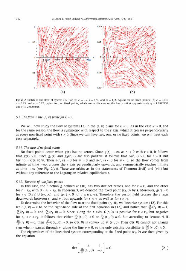
Fig. 2. A sketch of the flow of system (12) for (a) κ = −2, c = 1/3, and m = 1/2, typical for no fixed points; (b) κ = −0.3,c = 0.23, and m = 0.12, typical for two fixed points, which are in this case on the line ν = 0 at approximately r1 = 1.0882233and r2 = 2.0007055.

5.1. The flow in the (r, ν) plane for κ < 0

We will now study the flow of system (12) in the (r, ν) plane for κ < 0. As in the case κ > 0, andfor the same reason, the flow is symmetric with respect to the r axis, which it crosses perpendicularlyat every non-fixed point with r > 0. Since we can have two, one, or no fixed points, we will treat eachcase separately.

5.1.1. The case of no fixed pointsNo fixed points occur when g(r) has no zeroes. Since g(r) → ∞ as r → 0 with r > 0, it follows

that g(r) > 0. Since g1(r) and g2(r, ν) are also positive, it follows that G(r, ν) > 0 for r > 0. Buth(r, ν) = G(r, ν)/ν . Then h(r, ν) > 0 for ν > 0 and h(r, ν) < 0 for ν < 0, so the flow comes frominfinity at time −∞, crosses the r axis perpendicularly upwards, and symmetrically reaches infinityat time +∞ (see Fig. 2(a)). These are orbits as in the statements of Theorem 3(vii) and (viii) butwithout any reference to the Lagrangian relative equilibrium s.

5.1.2. The case of two fixed pointsIn this case, the function g defined at (16) has two distinct zeroes, one for r = r1 and the other

for r = r2, with 0 < r1 < r2. In Theorem 3, we denoted the fixed point (r2,0) by s. Moreover, g(r) > 0for r ∈ (0, r1) ∪ (r2,∞), and g(r) < 0 for r ∈ (r1, r2). Therefore the vector field crosses the r axisdownwards between r1 and r2, but upwards for r < r1 as well as for r > r2.

To determine the behavior of the flow near the fixed point (r1,0), we linearize system (12). For thislet F (r, ν) = ν to be the right-hand side of the first equation in (12), and notice that ∂ F

∂r (r1,0) = 1,∂ F∂ν (r1,0) = 0, and ∂G

∂ν (r1,0) = 0. Since, along the r axis, G(r,0) is positive for r < r1, but negativefor r1 < r < r2, it follows that either ∂G

∂r (r1,0) < 0 or ∂G∂r (r1,0) = 0. But according to Lemma 4, if

∂G∂r (r1,0) = 0, then ∂2

∂r2 G(r∗,0) > 0, so G(r,0) is convex up at (r1,0). Then G(r,0) cannot not change

sign when r passes through r1 along the line ν = 0, so the only existing possibility is ∂G∂r (r1,0) < 0.

The eigenvalues of the linearized system corresponding to the fixed point (r1,0) are then given bythe equation

det

[ −λ 1∂G (r ,0) −λ

]= 0. (21)

∂r 1


Since ∂G∂r (r1,0) is negative, the eigenvalues are purely imaginary, so (r1,0) is not a hyperbolic fixed

point for Eqs. (12). Therefore this fixed point could be a spiral sink, a spiral source, or a center forthe nonlinear system. But the symmetry of the flow of system (12) with respect to the r axis, and thefact that, near r1, the flow crosses the r axis upwards to the left of r1, and downwards to the rightof r1, eliminates the possibility of spiral behavior, so (r1,0) is a center (see Fig. 2(b)).

We can understand the generic behavior of the flow near the isolated fixed point (r2,0) throughlinearization as well. For this purpose, notice that ∂ F

∂r (r2,0) = 1, ∂ F∂ν (r2,0) = 0, and ∂G

∂ν (r2,0) = 0. Since,along the r axis, G(r) is negative for r1 < r < r2, but positive for r > r2, it follows that ∂G

∂r (r2,0) > 0or ∂G

∂r (r2,0) = 0. But using Lemma 4 the same way we did above for the fixed point (r1,0), we canconclude that the only possibility is ∂G

∂r (r2,0) > 0.The eigenvalues corresponding to the fixed point (r2,0) are given by the equation

det

[ −λ 1∂G∂r (r2,0) −λ

]= 0. (22)

Consequently the fixed point (r2,0) is hyperbolic, its two eigenvalues are λ1 > 0 and λ2 < 0, so (r2,0)

is a saddle.Indeed, for small ν > 0, the slope of the vector field decreases to −∞ on lines r = constant, with

r1 < r < r2, when ν tends to 0. On the same lines, with r > r2, the slope decreases from +∞ as νincreases. This behavior gives us an approximate idea of how the eigenvectors corresponding to theeigenvalues λ1 and λ2 are positioned in the rν plane.

On lines of the form ν = ηr, with η > 0, the slope h(r, ν) of the vector field becomes

h(r, ηr) = 1 − κr2

ηr3

[c2

r− 24m(1 − κr2)

(12 − 9κr2)3/2

]− κηr2

1 − κr2.

So, as r tends to ∞, the slope h(r, ηr) tends to η. Consequently the vector field doesn’t bound theflow with negative slopes, and thus allows it to go to infinity.

With the fixed point (r1,0) as a center, the fixed point (r2,0) as a saddle, and a vector field thatdoesn’t bound the orbits as r → ∞, the flow must behave qualitatively as in Fig. 2(b).

This behavior of the flow proves the existence of the following types of solutions:(a) periodic orbits around the fixed point (r1,0), corresponding to Theorem 3(iii);(b) a homoclinic orbit to the fixed point (r1,0), corresponding to Theorem 3(iv);(c) an orbit that tends to the fixed point (r2,0), corresponding to Theorem 3(v);(d) an orbit that is ejected from the fixed point (r2,0), corresponding to Theorem 3(vi);(e) orbits that come from infinity in the direction of the stable manifold of (r2,0) and inside it,

hit the r axis to the right of r2, and return symmetrically to infinity in the direction of the unstablemanifold of (r2,0); these orbits correspond to Theorem 3(vii);

(f) orbits that come from infinity in the direction of the stable manifold of (r2,0) and outside it,turn around the homoclinic loop, and return symmetrically to infinity in the direction of the unstablemanifold of (r2,0); since such an orbit hits the r axis at a point between 0 and r1, its minimumsize is, for given κ , m, and c, smaller than the corresponding orbit described in Theorem 3(ii); thesesolutions correspond to Theorem 3(viii).

Since no other orbits show up, the proof of this case is complete.

5.1.3. The case of one fixed pointWe left the case of one fixed point at the end because it is non-generic. It occurs when the two

fixed points of the previous case overlap. Let us denote this fixed point by (r0,0). Then the functiong(r) is positive everywhere except at the fixed point, where it is zero. So near r0, g is decreas-ing for r < r0 and increasing for r > r0, and the r axis is tangent to the graph of g . Consequently,∂G∂r (r0,0) = 0, and the eigenvalues obtained from Eq. (21) are λ1 = λ2 = 0. In this degenerate case,

the orbits near the fixed point influence the asymptotic behavior of the flow at (r0,0). Since the flowaway from the fixed point looks very much like in the case of no fixed points, the only difference


between the flow sketched in Fig. 2(a) and the current case is that at least an orbit ends at (r0,0),and at least another orbit one ejects from it. These orbits are described in Theorem 3(iv) and (v).

The proof of Theorem 3 is now complete.

6. Mass equality of Lagrangian solutions

In this section we show that all Lagrangian solutions that satisfy Definition 1 must have equalmasses. In other words, we will prove the following result:

Theorem 4. In the curved 3-body problem, the bodies of masses m1 , m2 , m3 can lead to a Lagrangian solutionif and only if m1 = m2 = m3 .

Proof. The fact that three bodies of equal masses can lead to Lagrangian solutions for suitable initialconditions was proved in Theorem 1. So we will further prove that Lagrangian solutions can occuronly if the masses are equal. Since the case of relative equilibria was settled in [3], we need toconsider only the Lagrangian orbits that are not relative equilibria. This means we can treat only thecase when r(t) is not constant. Recall also that the Lagrangian orbits were defined to form a triangleorthogonal to the z axis.

Assume now that the masses are m1,m2,m3, and substitute a solution of the form

x1 = r cosω, y1 = r sinω, z1 = (σκ−1 − σ r2)1/2,

x2 = r cos(ω + 2π/3), y2 = r sin(ω + 2π/3), z2 = (σκ−1 − σ r2)1/2,

x3 = r cos(ω + 4π/3), y3 = r sin(ω + 4π/3), z3 = (σκ−1 − σ r2)1/2

into the equations of motion. Computations and a reasoning similar to the ones performed in theproof of Theorem 1 lead us to the system:

r − r(1 − κr2)ω2 + κrr2

1 − κr2+ 12(m1 + m2)(1 − κr2)

r2(12 − 9κr2)3/2= 0,

r − r(1 − κr2)ω2 + κrr2

1 − κr2+ 12(m2 + m3)(1 − κr2)

r2(12 − 9κr2)3/2= 0,

r − r(1 − κr2)ω2 + κrr2

1 − κr2+ 12(m3 + m1)(1 − κr2)

r2(12 − 9κr2)3/2= 0,

rω + 2rω − 4√

3(m1 − m2)

r2(12 − 9κr2)3/2= 0,

rω + 2rω − 4√

3(m2 − m3)

r2(12 − 9κr2)3/2= 0,

rω + 2rω − 4√

3(m3 − m1)

r2(12 − 9κr2)3/2= 0,

which, obviously, can have solutions only if m1 = m2 = m3. This conclusion completes the proof. �7. Local existence and uniqueness of Eulerian solutions

In this section we define the Eulerian solutions of the curved 3-body problem and prove their localexistence for suitable initial conditions in the case of equal masses.


Definition 4. A solution of Eqs. (8) is called Eulerian if, at every time instant, the bodies are on ageodesic that contains the point (0,0, |κ |−1/2|).

Unlike the orthogonality condition imposed in Definition 1, the requirement of Definition 4 thatthe geodesic contains a certain point is not restrictive, but rather a normalization, which provides amore convenient setting.

According to Definition 4, the size of an Eulerian solution may change, but the particles are alwayson a (possibly rotating) geodesic. If the masses are equal, it is natural to assume that one body lies atthe point (0,0, |κ |−1/2|), while the other two bodies find themselves at diametrically opposed pointsof a circle. Thus, in the case of equal masses, which we further consider, we ask that the movingbodies have the same coordinate z, which may vary in time.

We can thus represent such an Eulerian solution of the curved 3-body problem in the form

q = (q1,q2,q3), with qi = (xi, yi, zi), i = 1,2,3, (23)

x1 = 0, y1 = 0, z1 = (σκ)−1/2,

x2 = r cosω, y2 = r sinω, z2 = z,

x3 = −r cosω, y3 = −r sinω, z3 = z,

where z = z(t) satisfies z2 = σκ−1 − σ r2 = (σκ)−1(1 − κr2); σ is the signature function definedin (1); r := r(t) is the size function; and ω := ω(t) is the angular function.

Notice that, for every time t , we have x2i (t)+ y2

i (t)+σ z2i (t) = κ−1, i = 1,2,3, which means that the

bodies stay on the surface M2κ . Eqs. (23) also express the fact that the bodies are on the same (possibly

rotating) geodesic. Therefore representation (23) of the Eulerian orbits agrees with Definition 4 in thecase of equal masses.

Definition 5. An Eulerian solution of Eqs. (8) is called Eulerian homothetic if the configuration expandsor contracts, but does not rotate.

In terms of representation (23), an Eulerian homothetic orbit for equal masses occurs when ω(t)is constant, but r(t) is not constant. If, for instance, all three bodies are initially in the same openhemisphere, while the two moving bodies have the same mass and the same z coordinate, and arereleased with zero initial velocities, then we are led to an Eulerian homothetic orbit that ends in atriple collision.

Definition 6. An Eulerian solution of Eqs. (8) is called an Eulerian relative equilibrium if the configu-ration of the system rotates without expanding or contracting.

In terms of representation (23), an Eulerian relative equilibrium orbit occurs when r(t) is con-stant, but ω(t) is not constant. Of course, Eulerian homothetic solutions and elliptic Eulerian relativeequilibria, whose existence we proved in [3], are particular Eulerian orbits, but we expect that theEulerian orbits are not reduced to them. We now show this fact by proving the local existence anduniqueness of Eulerian solutions that are neither Eulerian homothetic, nor Eulerian relative equilibria.

Theorem 5. In the curved 3-body problem of equal masses, m1 = m2 = m3 := m > 0, for every set of initialconditions belonging to a certain class, the local existence and uniqueness of an Eulerian solution, which bothrotates and changes size, is assured.

Proof. To check whether Eqs. (8) admit solutions of the form (23) that start in the region z > 0 andfor which both r(t) and ω(t) are not constant, we first compute that


κq1 � q2 = κq1 � q3 = (1 − κr2)1/2

,

κq2 � q3 = 1 − 2κr2,

x1 = 0, y1 = 0,

x2 = r cosω − rω sinω, y2 = r sinω + rω cosω,

x3 = −r cosω + rω sinω, y2 = −r sinω − rω cosω,

z1 = 0, z2 = z3 = − σ rr

(σκ)1/2(1 − κr2)1/2,

κ q1 � q1 = 0,

κ q2 � q2 = κ q3 � q3 = κr2ω2 + κ r2

1 − κr2,

x1 = y1 = z1 = 0,

x2 = (r − rω2) cosω − (rω + 2rω) sinω,

y2 = (r − rω2) sinω + (rω + 2rω) cosω,

x3 = −(r − rω2) cosω + (rω + 2rω) sinω,

y3 = −(r − rω2) sinω − (rω + 2rω) cosω,

z2 = z3 = −σ rr(σκ−1 − σ r2)−1/2 − κ−1r2(σκ−1 − σ r2)−3/2

.

Substituting these expressions into Eqs. (8), we are led to the system below, where the double-dotterms on the left indicate to which differential equation each algebraic equation corresponds:

x2, x3: C cosω − D sinω = 0,

y2, y3: C sinω + D cosω = 0,

z2, z3: C = 0,

where

C := C(t) = r − r(1 − κr2)ω2 + κrr2

1 − κr2+ m(5 − 4κr2)

4r2(1 − κr2)1/2,

D := D(t) = rω + 2rω.

(The equations corresponding to x1, y1, and z1 are identities, so they don’t show up). The above sys-tem has solutions if and only if C = D = 0, which means that the existence of Eulerian homographicorbits of the curved 3-body problem with equal masses is equivalent to the existence of solutions ofthe system of differential equations:⎧⎪⎪⎪⎪⎨⎪⎪⎪⎪⎩

r = ν,

w = −2νw

r,

ν = r(1 − κr2)w2 − κrν2

2− m(5 − 4κr2)

2 2 1/2,

(24)

1 − κr 4r (1 − κr )


with initial conditions r(0) = r0, w(0) = w0, ν(0) = ν0, where w = ω. The functions r, ω, and w areanalytic, and as long as the initial conditions satisfy the conditions r0 > 0 for all κ , as well as r0 <

κ−1/2 for κ > 0, standard results of the theory of differential equations guarantee the local existenceand uniqueness of a solution (r, w, ν) of Eqs. (24), and therefore the local existence and uniquenessof an Eulerian orbit with r(t) and ω(t) not constant. This conclusion completes the proof. �8. Classification of Eulerian solutions for κ > 0


Theorem 6. In the curved 3-body problem with equal masses, m1 = m2 = m3 := m > 0, and κ > 0 there arethree classes of Eulerian solutions:

(i) homothetic orbits that begin or end in total collision in finite time;(ii) relative equilibria, for which one mass is fixed at one pole of the sphere while the other two move on a

circle parallel with the xy plane;(iii) periodic homographic orbits that change size.

None of the above orbits can cross the equator, defined as the great circle orthogonal to the z axis.

The rest of this section is dedicated to the proof of this theorem.Let us start by noticing that the first two equations of system (24) imply that w = − 2r w

r , whichleads to

w = c

r2,

where c is a constant. The case c = 0 can occur only when w = 0, which means ω = 0. Under thesecircumstances the angular velocity is zero, so the motion is homothetic. The existence of these orbitsis stated in Theorem 6(i). They occur only when the angular momentum is zero, and lead to a triplecollision in the future or in the past, depending on the direction of the velocity vectors. The existenceof the orbits described in Theorem 6(ii) was proved in [3].

For the rest of this section, we assume that c �= 0. System (24) is thus reduced to⎧⎨⎩r = ν,

ν = c2(1 − κr2)

r3− κrν2

1 − κr2− m(5 − 4κr2)

4r2(1 − κr2)1/2.

(25)

To address the existence of the orbits described in Theorem 6(iii), and show that no other Eulerianorbits than those of Theorem 6 exist for κ > 0, we need to study the flow of system (25) for κ > 0.Let us first prove the following fact:

Lemma 5. Regardless of the values of the parameters m, κ > 0, and c �= 0, system (25) has one fixed point(r0,0) with 0 < r0 < κ−1/2 .

Proof. The fixed points of system (25) are of the form (r,0) for all values of r that are zeroes of u(r),where

u(r) = c2(1 − κr2)

r− m(5 − 4κr2)

4(1 − κr2)1/2. (26)

But finding the zeroes of u(r) is equivalent to obtaining the roots of the polynomial

16κ2(c4κ + m2)r6 − 8κ(6c4κ + 5m2)r4 + (

48c4κ + 25m2)r2 − 16c4.


Denoting x = r2, this polynomial becomes

q(x) = 16κ2(c4κ + m2)x3 − 8κ(6c4κ + 5m2)x2 + (

48c4κ + 25m2)x − 16c4.

Since κ > 0, Descarte’s rule of signs implies that q can have one or three positive roots. The derivativeof q is the polynomial

q′(x) = 48κ2(c4κ + m2)x2 − 16κ(6c4κ + 5m2)x + 48c4κ + 25m2, (27)

whose discriminant is 64κ2m2(21c4κ + 25m2). But, as κ > 0, this discriminant is always positive, soit offers no additional information on the total number of positive roots.

To determine the exact number of positive roots, we will use the resultant of two polynomials.Denoting by ai , i = 1,2, . . . , ζ, the roots of a polynomial P , and by b j , j = 1,2, . . . , ξ , those of apolynomial Q , the resultant of P and Q is defined by the expression

Res(P , Q ) =ζ∏

i=1

ξ∏j=1

(ai − b j).

Then P and Q have a common root if and only if Res[P , Q ] = 0. Consequently the resultant of q andq′ is a polynomial in κ, c, and m whose zeroes are the double roots of q. But

Res(q,q′) = 1024c4κ5m4(c4κ + m2)(108c4κ + 125m2).

Then, for m, κ > 0 and c �= 0, Res[q,q′] never cancels, therefore q has exactly one positive root. Indeed,should q have three positive roots, a continuous variation of κ , m, and c, would lead to some valuesof the parameters that correspond to a double root. Since double roots are impossible, the existenceof a unique equilibrium (r0,0) with r0 > 0 is proved. To conclude that r0 < κ−1/2 for all m, κ > 0and c �= 0, it is enough to notice that limr→0 u(r) = +∞ and limr→κ−1/2 u(r) = −∞. This conclusioncompletes the proof. �8.1. The flow in the (r, ν) plane for κ > 0

We can now study the flow of system (25) in the (r, ν) plane for κ > 0. The vector field is notdefined along the lines r = 0 and r = κ−1/2, so it lies in the band (0, κ−1/2) × R. Consider now theslope dν

dr of the vector field. This slope is given by the ratio νr = v(r, ν), where

v(r, ν) = c2(1 − κr2)

νr3− κrν

1 − κr2− m(5 − 4κr2)

4νr2(1 − κr2)1/2. (28)

But v is odd with respect to ν , i.e. v(r,−ν) = −v(r, ν), so the vector field is symmetric with respectto the r axis.

Since limr→0 v(r) = +∞ and limr→κ−1/2 v(r) = −∞, the flow crosses the r axis perpendicularlyupwards to the left of r0 and downwards to its right, where (r0,0) is the fixed point of the sys-tem (25) whose existence and uniqueness we proved in Lemma 5. But the right-hand side of thesecond equation in (25) is of the form

W (r, ν) = u(r)/r2 + g2(r, ν), (29)

where g2 was defined earlier as g2(r, ν) = − κrν2

1−κr2 , while u(r) was defined in (26). Notice that

limr→0

W (r, ν) = +∞ and lim−1/2

W (r, ν) = −∞.
r→κ


Fig. 3. A sketch of the flow of system (25) for κ = 1, c = 2, and m = 2, typical for Eulerian solutions with κ > 0.

Moreover, W (r0,0) = 0, and W has no singularities for r ∈ (0, κ−1/2). Therefore the flow that entersthe region ν > 0 to the left of r0 must exit it to the right of the fixed point. The symmetry withrespect to the r axis forces all orbits to be periodic around (r0,0) (see Fig. 3). This proves the existenceof the solutions described in Theorem 6(iii), and shows that no orbits other than those in Theorem 6occur for κ > 0. The proof of Theorem 6 is now complete.

9. Classification of Eulerian solutions for κ < 0


Theorem 7. In the curved 3-body problem with equal masses, m1 = m2 = m3 := m > 0, and κ > 0 there arefour classes of Eulerian solutions:

(i) Eulerian homothetic orbits that begin or end in total collision in finite time;(ii) Eulerian relative equilibria, for which one mass is fixed at the vertex of the hyperboloid while the other

two move on a circle parallel with the xy plane;(iii) Eulerian periodic orbits that change size; the line connecting the two moving bodies is always parallel

with the xy plane, but their z coordinate changes in time;(iv) Eulerian orbits that come from infinity at time −∞, reach a position when the size of the configuration is

minimal, and then return to infinity at time +∞.

The rest of this section is dedicated to the proof of this theorem.The homothetic orbits of the type stated in Theorem 7(i) occur only when c = 0. Then the two

moving bodies collide simultaneously with the fixed one in the future or in the past. Depending onthe initial conditions, the motion can be bounded or unbounded.

The existence of the orbits stated in Theorem 7(ii) was proved in [3]. To prove the existence of thesolutions stated in Theorem 7(iii) and (iv), and show that there are no other kinds of orbits, we startwith the following result:

Lemma 6. In the curved three body problem with κ < 0, the polynomial q defined in the proof of Lemma 5 hasno positive roots for c4κ + m2 � 0, but has exactly one positive root for c4κ + m2 > 0.

Proof. We split our analysis in three different cases depending on the sign of c4κ + m2:(1) c4κ + m2 = 0. In this case q has form 8κm2x2 + 23c4κx − 16c4, a polynomial that does not

have any positive root.


(2) c4κ +m2 < 0. Writing 6c4κ +5m2 = 6(c4κ +m2)−m2, we see that the term of q correspondingto x2 is always negative, so by Descartes’s rule of signs the number of positive roots depends on thesign of the coefficient corresponding to x, i.e. 48c4κ + 25m2 = 48(c4κ + m2) − 23m2, which is alsonegative, and therefore q has no positive root.

(3) c4κ + m2 > 0. This case leads to three subcases:– if 6c4κ + 5m2 < 0, then necessarily 48c4κ + 25m2 < 0 and, so q has exactly one positive root;– if 6c4κ + 5m2 > 0 and 48c4κ + 25m2 < 0, then q has one change of sign and therefore exactly

one positive root;– if 48c4κ + 25m2 > 0, then all coefficients, except for the free term, are positive, therefore q has

exactly one positive root.These conclusions complete the proof. �The following result will be used towards understanding the case when system (25) has one fixed

point.

Lemma 7. Regardless of the values of the parameters κ < 0, m > 0, and c �= 0, there is no fixed point, (r∗,0),of system (25) for which ∂

∂r W (r∗,0) = 0, where W is defined in (29).

Proof. Since u(r∗) = 0, ∂∂r g2(r∗,0) = 0, and

∂W

∂r(r, ν) = −(

2/r3)u(r) + (1/r2) d

dru(r) + ∂

∂rg2(r, ν),

it means that W (r∗,0) = 0 if and only if ddr u(r∗) = 0. Consequently our result would follow if we can

prove that there is no fixed point (r∗,0) for which ddr u(r∗) = 0. To show this fact, notice first that

d

dru(r) = −c2(1 + κr2)

r2− κmr(4κr2 − 3)

4(1 − κr2)3/2. (30)

From the definition of u(r) in (26), the identity u(r∗) = 0 is equivalent to

(1 − κr2∗

)1/2 = mr∗(5 − 4κr2∗)4c2(1 − κr2∗)

.

Regarding (1 − κr2)3/2 as (1 − κr2)1/2(1 − κr2), and substituting the above expression of (1 − κr2∗)1/2

into (30) for r = r∗ , we obtain that

κ(4κr2∗ − 3)

5 − 4κr2∗+ 1 + κr2∗

r2∗= 0,

which leads to the conclusion that r2∗ = 5/2κ < 0. Therefore there is no fixed point (r∗,0) such thatddr u(r∗) = 0. This conclusion completes the proof. �9.1. The flow in the (r, ν) plane for κ < 0

To study the flow of system (25) for κ < 0, we will consider the two cases given by Lemma 6,namely when system (25) has no fixed points and when it has exactly one fixed point.


Fig. 4. A sketch of the flow of system (25) for (a) κ = −2, c = 2, and m = 4, typical for no fixed points; (b) κ = −2, c = 2, andm = 6.2, typical for one fixed point.

9.1.1. The case of no fixed pointsSince κ < 0, and system (25) has no fixed points, the function u(r), defined in (26), has no

zeroes. But limr→0 u(r) = +∞, so u(r) > 0 for all r > 0. Then u(r)/r2 > 0 for all r > 0. Sincelimr→0 g2(r, ν) = 0, it follows that limr→0 W (r, ν) = +∞, where W (r, ν) (defined in (29)) formsthe right-hand side of the second equation in system (25). Since system (25) has no fixed points,W doesn’t vanish. Therefore W (r, ν) > 0 for all r > 0 and ν .

Notice that the slope of the vector field, v(r, ν), defined in (28), is of the form v(r, ν) = W (r, ν)/ν ,which implies that the flow crosses the r axis perpendicularly at every point with r > 0. Also, for rfixed, limν→±∞ W (r, ν) = +∞. Moreover, for ν fixed, limr→∞ W (r, ν) = 0. This means that the flowhas a simple behavior as in Fig. 4(a). These orbits correspond to those stated in Theorem 7(iv).

9.1.2. The case of one fixed pointWe start with analyzing the behavior of the flow near the unique fixed point (r0,0). Let F (r, ν) = ν

denote the right-hand side in the first equation of system (25). Then ∂∂r F (r0,0) = 0, ∂

∂ν F (r0,0) = 1,and ∂

∂ν W (r0,0) = 0. To determine the sign of ∂∂r W (r0,0), notice first that limr→0 W (r, ν) = +∞.

Since the equation W (r, ν) = 0 has a single root of the form (r0,0), with r0 > 0, it follows thatW (r,0) > 0 for 0 < r < r0.

To show that W (r,0) < 0 for r > r0, assume the contrary, which (given the fact that r0 is the onlyzero of W (r,0)) means that W (r,0) > 0 for r > r0. So W (r,0) � 0, with equality only for r = r0.But recall that we are in the case when the parameters satisfy the inequality c4κ + m2 > 0. Then aslight variation of the parameters κ < 0, m > 0, and c �= 0, within the region defined by the aboveinequality, leads to two zeroes for W (r,0), a fact which contradicts Lemma 6. Therefore, necessarily,W (r,0) < 0 for r > r0.

Consequently W (r,0) is decreasing in a small neighborhood of r0, so ∂∂r W (r0,0) � 0. But by

Lemma 7, ∂∂r W (r0,0) �= 0, so necessarily ∂

∂r W (r0,0) < 0. The eigenvalues corresponding to the systemobtained by linearizing Eqs. (25) around the fixed point (r0,0) are given by the equation

det

[ −λ 1∂W∂r (r0,0) −λ

]= 0, (31)

so these eigenvalues are purely imaginary. In terms of system (25), this means that the fixed point(r0,0) could be a spiral sink, a spiral source, or a center. The symmetry of the flow with respectto the r axis excludes the first two possibilities, consequently (r0,0) is a center (see Fig. 4(b)). We


thus proved that, in a neighborhood of this fixed point, there exist infinitely many periodic Euleriansolutions whose existence was stated in Theorem 7(iii).

To complete the analysis of the flow of system (25), we will use the nullcline ν = 0, which is givenby the equation

ν2 = 1 − κr2

κr

[c2(1 − κr2)

r3− m(5 − 4κ2)

4r2(1 − κr2)1/2

]. (32)

Along this curve, which passes through the fixed point (r0,0), and is symmetric with respect to the raxis, the vector field has slope zero. To understand the qualitative behavior of this curve, notice that

limr→∞

1 − κr2

κr

[c2(1 − κr2)

r3− m(5 − 4κ2)

4r2(1 − κr2)1/2

]= m(−κ)1/2 + κc2.

But we are restricted to the parameter region given by the inequality m2 + κc4 > 0, which is equiva-lent to [

m(−κ)1/2 − (−κ)c2][m(−κ)1/2 + (−κ)c2] > 0.

Since the second factor of this product is positive, it follows that the first factor must be positive,therefore the above limit is positive. Consequently the curve given in (32) is bounded by the horizon-tal lines

ν = [m(−κ)1/2 + κc2]1/2

and ν = −[m(−κ)1/2 + κc2]1/2

.

Inside the curve, the vector field has negative slope for ν > 0 and positive slope for ν < 0. Outsidethe curve, the vector field has positive slope for ν > 0, but negative slope for ν < 0. So the orbitsof the flow that stay outside the nullcline curve are unbounded. They correspond to solutions whoseexistence was stated in Theorem 7(iv). This conclusion completes the proof of Theorem 7.

10. Hyperbolic homographic solutions

In this last section we consider a certain class of homographic orbits, which occur only in spacesof negative curvature. They are related to hyperbolic rotations. More precisely, the Principal Axis The-orem for hyperbolic space (see [7,9], and the appendix of [3]) states that, in a convenient basis,a hyperbolic rotation can be given by a matrix of the form[1 0 0

0 cosh s sinh s0 sinh s cosh s

],

where s is a fixed real value. In the case κ = −1, we proved in [3] the existence of hyperbolic Eulerianrelative equilibria of the curved 3-body problem with equal masses. These orbits behave as follows:three bodies of equal masses move along three fixed hyperbolas, each body on one of them; the mid-dle hyperbola, which is a geodesic passing through the vertex of the hyperboloid, lies in a plane of R

3

that is parallel and equidistant from the planes containing the other two hyperbolas, none of whichis a geodesic. At every moment in time, the bodies lie equidistantly from each other on a geodesichyperbola that rotates hyperbolically. These solutions are the hyperbolic counterpart of Eulerian solu-tions, in the sense that the bodies stay on the same geodesic, which rotates hyperbolically, instead ofcircularly. The existence proof we gave in [3] works for any κ < 0. We therefore provide the followingdefinitions.


Definition 7. A solution of the curved 3-body problem is called hyperbolic homographic if the bodiesmaintain a configuration similar to itself while rotating hyperbolically. When the bodies remain onthe same hyperbolically rotating geodesic, the solution is called hyperbolic Eulerian.

While there is, so far, no evidence of hyperbolic non-Eulerian homographic solutions, we showedin [3] that hyperbolic Eulerian orbits exist in the case of equal masses. In the particular case of equalmasses, it is natural to assume that the middle body moves on a geodesic passing through the point(0,0, |κ |−1/2) (the vertex of the hyperboloid’s upper sheet), while the other two bodies are on thesame (hyperbolically rotating) geodesic, and equidistant from it.

Consequently we can seek hyperbolic Eulerian solutions of equal masses of the form:

q = (q1,q2,q3), with qi = (xi, yi, zi), i = 1,2,3, and (33)

x1 = 0, y1 = |κ |−1/2 sinhω, z1 = |κ |−1/2 coshω,

x2 = (ρ2 + κ−1)1/2

, y2 = ρ sinhω, z2 = ρ coshω,

x3 = −(ρ2 + κ−1)1/2

, y3 = ρ sinhω, z3 = ρ coshω,

where ρ := ρ(t) is the size function and ω := ω(t) is the angular function.Indeed, for every time t , we have that x2

i (t)+ y2i (t)− z2

i (t) = κ−1, i = 1,2,3, which means that thebodies stay on the surface H2

κ , while lying on the same, possibly (hyperbolically) rotating, geodesic.Therefore representation (33) of the hyperbolic Eulerian homographic orbits agrees with Definition 7.

With the help of this analytic representation, we can define Eulerian homothetic orbits and hyper-bolic Eulerian relative equilibria.

Definition 8. A hyperbolic Eulerian homographic solution is called Eulerian homothetic if the config-uration of the system expands or contracts, but does not rotate hyperbolically.

In terms of representation (33), an Eulerian homothetic solution occurs when ω(t) is constant,but ρ(t) is not constant. A straightforward computation shows that if ω(t) is constant, the bodieslie initially on a geodesic, and the initial velocities are such that the bodies move along the geodesictowards or away from a triple collision at the point occupied by the fixed body.

Notice that Definition 8 leads to the same orbits produced by Definition 5. While the configurationof the former solution does not rotate hyperbolically, and the configuration of the latter solutiondoes not rotate elliptically, both fail to rotate while expanding or contracting. This is the reason whyDefinitions 5 and 8 use the same name (Eulerian homothetic) for these types of orbits.

Definition 9. A hyperbolic Eulerian homographic solution is called a hyperbolic Eulerian relative equi-librium if the configuration rotates hyperbolically while its size remains constant.

In terms of representation (33), hyperbolic Eulerian relative equilibria occur when ρ(t) is constant,while ω(t) is not constant.

Unlike for Lagrangian and Eulerian solutions, hyperbolic Eulerian homographic orbits exist onlyin the form of homothetic solutions or relative equilibria. As we will further prove, any compositionbetween a homothetic orbit and a relative equilibrium fails to be a solution of system (8).

Theorem 8. In the curved 3-body problem of equal masses, m1 = m2 = m3 := m, and κ < 0, the only hy-perbolic Eulerian homographic solutions are either Eulerian homothetic orbits or hyperbolic Eulerian relativeequilibria.


Proof. Consider for system (8) a solution of the form (33) that is not homothetic. Then

κq1 � q2 = κq1 � q3 = |κ |1/2ρ,

κq2 � q3 = −1 − 2κρ2,

x1 = x1 = 0, y1 = |κ |−1/2ω coshω, z1 = |κ |−1/2 sinhω,

x2 = −x3 = ρρ

(ρ2 + κ−1)1/2,

y2 = y3 = ρ sinhω + ρω coshω,

z2 = z3 = ρ coshω + ρω sinhω,

κ q2 � q2 = −ω2, κ q2 � q2 = κ q3 � q3 = κρ2ω2 − κρ2

1 + κρ2,

x2 = −x3 = ρρ

(ρ2 + κ−1)1/2+ κ−1ρ2

(ρ2 + κ−1)3/2,

y2 = y3 = (ρ + ρω2) sinhω + (ρω + 2ρω) coshω,

z2 = z3 = (ρ + ρω2) coshω + (ρω + 2ρω) sinhω.

Substituting these expressions in system (8), we are led to an identity corresponding to x1. The otherequations lead to the system

x2, x3: E = 0,

y1: |κ |−1/2ω coshω = 0,

z1: |κ |−1/2ω sinhω = 0,

y2, y3: E sinhω + F coshω = 0,

z2, z3: E coshω + F sinhω = 0,

where

E := E(t) = ρ + ρ(1 + κρ2)ω2 − κρρ2

1 + κρ2+ m(1 − 4κρ2)

4ρ2|1 + κρ2|1/2,

F := F (t) = ρω + 2ρω.

This system can be obviously satisfied only if

⎧⎪⎪⎪⎪⎨⎪⎪⎪⎪⎩ω = 0,

ω = −2ρω

ρ,

ρ = −ρ(1 + κρ2)ω2 + κρρ2

1 + κρ2− m(1 + 4κρ2)

4ρ2|1 + κρ2|1/2.

(34)


The first equation implies that ω(t) = at +b, where a and b are constants, which means that ω(t) = a.Since we assumed that the solution is not homothetic, we necessarily have a �= 0. But from the secondequation, we can conclude that

ω(t) = c

ρ2(t),

where c is a constant. Since a �= 0, it follows that ρ(t) is constant, which means that the homographicsolution is a relative equilibrium. This conclusion is also satisfied by the third equation, which reducesto

a2 = ω2 = m(1 − 4κρ)

4ρ3|1 + κρ2|1/2,

being verified by two values of a (equal in absolute value, but of opposite signs) for every κ and ρfixed. Therefore every hyperbolic Eulerian homographic solution that is not Eulerian homothetic is ahyperbolic Eulerian relative equilibrium. This conclusion completes the proof. �

Since a slight perturbation of hyperbolic Eulerian relative equilibria, within the set of hyperbolicEulerian homographic solutions, produces no orbits with variable size, it means that hyperbolic Eu-lerian relative equilibria of equal masses are unstable. Therefore though they exist in a mathematicalsense, as proved above (as well as in [3], using a direct method), such equal-mass orbits are unlikelyto be found in a (hypothetical) hyperbolic physical universe.

Acknowledgments

Florin Diacu was supported by an NSERC Discovery Grant, while Ernesto Pérez-Chavela enjoyed thefinancial support of CONACYT.

References

[1] J.F. Cariñena, M.F. Rañada, M. Santander, Central potentials on spaces of constant curvature: The Kepler problem on thetwo-dimensional sphere S2 and the hyperbolic plane H2, J. Math. Phys. 46 (2005) 052702.

[2] F. Diacu, Near-collision dynamics for particle systems with quasihomogeneous potentials, J. Differential Equations 128(1996) 58–77.

[3] F. Diacu, E. Pérez-Chavela, M. Santoprete, The n-body problem in spaces of constant curvature, arXiv:0807.1747, 2008,54 pp.

[4] F. Diacu, On the singularities of the curved n-body problem, Trans. Amer. Math. Soc., in press..[5] F. Diacu, E. Pérez-Chavela, M. Santoprete, Saari’s conjecture for the collinear n-body problem, Trans. Amer. Math.

Soc. 357 (10) (2005) 4215–4223.[6] F. Diacu, T. Fujiwara, E. Pérez-Chavela, M. Santoprete, Saari’s homographic conjecture of the 3-body problem, Trans. Amer.

Math. Soc. 360 (12) (2008) 6447–6473.[7] F. Dillen, W. Kühnel, Ruled Weingarten surfaces in Minkowski 3-space, Manuscripta Math. 98 (1999) 307–320.[8] A. Einstein, L. Infeld, B. Hoffmann, The gravitational equations and the problem of motion, Ann. of Math. 39 (1) (1938)

65–100.[9] J. Hano, K. Nomizu, On isometric immersions of the hyperbolic plane into the Lorentz–Minkovski space and the Monge–

Ampère equation of certain type, Math. Ann. 262 (1983) 245–253.[10] L. Infeld, On a new treatment of some eigenvalue problems, Phys. Rev. 59 (1941) 737–747.[11] L. Infeld, A. Schild, A note on the Kepler problem in a space of constant negative curvature, Phys. Rev. 67 (1945) 121–122.[12] W. Killing, Die Rechnung in den nichteuklidischen Raumformen, J. Reine Angew. Math. 89 (1880) 265–287.[13] W. Killing, Die Mechanik in den nichteuklidischen Raumformen, J. Reine Angew. Math. 98 (1885) 1–48.[14] W. Killing, Die Nicht-Eukildischen Raumformen in Analytischer Behandlung, Teubner, Leipzig, 1885.[15] T. Levi-Civita, The relativistic problem of several bodies, Amer. J. Math. 59 (1) (1937) 9–22.[16] T. Levi-Civita, Le problème des n corps en relativité générale, Gauthier–Villars, Paris, 1950; or the English translation: The

n-Body Problem in General Relativity, D. Reidel, Dordrecht, 1964.[17] H. Liebmann, Über die Zentralbewegung in der nichteuklidische Geometrie, Berichte Königl. Sächsischen Gesell. Wiss. Math.

Phys. Kl. 55 (1903) 146–153.[18] H. Liebmann, Nichteuklidische Geometrie, G.J. Göschen, Leipzig, 1905; second ed., G.J. Göschen, 1912; third ed., Walter de

Gruyter, Berlin, Leipzig, 1923.


[19] R. Lipschitz, Extension of the planet-problem to a space of n dimensions and constant integral curvature, Quart. J. PureAppl. Math. 12 (1873) 349–370.

[20] A.I. Miller, The myth of Gauss’s experiment on the Euclidean nature of physical space, Isis 63 (3) (1972) 345–348.[21] D. Saari, Collisions, Rings, and Other Newtonian N-Body Problems, CBMS Reg. Conf. Ser. Math., No. 104, American Mathe-

matical Society, Providence, RI, 2005.[22] E. Schering, Die Schwerkraft im Gaussischen Raume, Nachr. Königl. Gesell. Wiss. Göttingen 15 (1870) 311–321.[23] E. Schering, Die Schwerkraft in mehrfach ausgedehnten Gaussischen und Riemmanschen Räumen, Nachr. Königl. Gesell.

Wiss. Göttingen 6 (1873) 149–159.[24] E. Schrödinger, A method for determining quantum-mechanical eigenvalues and eigenfunctions, Proc. Roy. Irish Acad. Sect.

A 46 (1940) 9–16.[25] A. Wintner, The Analytical Foundations of Celestial Mechanics, Princeton University Press, Princeton, NJ, 1941.

Documents

· J. DifferentialEquations 250 (2011) 340–366 Contents lists available at ScienceDirect JournalofDifferentialEquations Homographicsolutionsofthecurved3