Embed Size (px)
Citation preview

NAIVE BAYES ALGORITHM FOR TWITTER SENTIMENT ANALYSIS AND ITS IMPLEMENTATION IN MAPREDUCE
A Thesis
Presented to
The Faculty of the Graduate School
At the University of Missouri
In Partial Fulfillment
Of the Requirements for the Degree
Master of Science
By
ZHAOYU LI
Dr. Yi Shang, Advisor
DEC 2014

The undersigned, appointed by the dean of the Graduate School, have examined the thesis entitled
NAIVE BAYES ALGORITHM FOR TWITTER SENTIMENT ANALYSIS AND ITS IMPLEMENTATION IN MAPREDUCE
Presented by Zhaoyu Li
A candidate for the degree of
Master of Science
And hereby certify that, in their opinion, it is worthy of acceptance.
Dr. Yi Shang
Dr. Dong Xu
Dr. Jeffrey Uhlmann

ACKNOWLEDGEMENTS
I would like to first thank my advisor, Dr. Yi Shang. He showed me how to do
research in computer science, and he always supported and inspired me through the
whole development of my thesis. He provided me many research ideas and helped me
produce solid works.
I would also like to thank other lab mates in Dr. Shang’s lab, both those who have
left and those who have just begun. I am glad that I have known them and I really
enjoyed their company along the way.
Finally I would like to thank my committee members Dr. Dong Xu and Dr.
Jeffrey Uhlmann for their support on this thesis.
ii

TABLE OF CONTENTS
Acknowledgements………………………………………………………………………..ii
List of Figures……………………………………………………………………………..v
Abstract…………………………………………………………………………………..vii
1 . INTRODUCTION.....................................................................................................................1
1.1 PROBLEM AND MOTIVATION..................................................................................................3
1.2 CONTRIBUTIONS......................................................................................................................3
1.3 THESIS ORGANIZATION...........................................................................................................4
2 . BACKGROUND AND RELATED WORK............................................................................6
2.1 TEXT CLASSIFICATION............................................................................................................6
2.1.1 Definition of Text Classification..................................................................................6
2.1.2 Process of Text Classification......................................................................................6
2.2 SENTIMENT ANALYSIS............................................................................................................8
2.2.1 Algorithms....................................................................................................................9
2.2.2 Twitter Sentiment Analysis and Stock Price..............................................................13
2.3 CURRENT DISTRIBUTED DATA PROCESSING SYSTEM..........................................................14
2.4 MAPREDUCE MODEL............................................................................................................14
2.5 AN OVERVIEW OF HADOOP MAPREDUCE CLUSTER............................................................16
2.5.1 Hadoop Cluster Infrastructure..................................................................................17
2.5.2 Hadoop Distributed File System (HDFS)..................................................................18
2.5.3 MapReduce................................................................................................................18
3 . NAIVE BAYES FOR TWITTER SENTIMENT ANALYSIS...........................................21
iii

3.1 GEOGRAPHICAL SENTIMENT AND STOCK PRICE...................................................................21
3.2 THE SOURCE DATA...............................................................................................................22
3.3 SYSTEM METHODS AND IMPLEMENTATION..........................................................................23
3.3.1 Three Layer Design...................................................................................................23
3.3.2 Stock Market Sector...................................................................................................24
3.3.3 Geographical Location..............................................................................................25
3.4 EXPERIMENTAL RESULTS......................................................................................................26
3.4.1 Result Representations...............................................................................................27
3.4.2 Analysis of the Results...............................................................................................28
4 . NAIVE BAYES MAPREDUCE IMPLEMENTATION.....................................................31
4.1 METHODS OVERVIEW...........................................................................................................31
4.2 DATA PRE-PROCESSING........................................................................................................32
4.3 PARALLEL NAIVE BAYES IN MAPREDUCE...........................................................................35
4.3.1 Algorithm Implementation.........................................................................................35
4.3.2 Algorithm Time Complexity.......................................................................................43
5 . EXPERIMENTAL RESULTS................................................................................................45
5.1 METRICS SUMMARY.............................................................................................................45
5.1.1 Terminologies............................................................................................................45
5.1.2 Impact of Node Number.............................................................................................47
5.1.3 Impact of Data Size....................................................................................................47
5.1.4 Impact of Global Counters........................................................................................47
5.2 EVALUATION SCENARIOS......................................................................................................48
5.2.1 Dataset.......................................................................................................................48
5.2.2 Hardware Configuration...........................................................................................48
iv

5.3 CPU TIME.............................................................................................................................51
5.4 DATA SIZE............................................................................................................................53
5.4.1 Total Execution Time.................................................................................................54
5.4.2 Total Slot Execution Time..........................................................................................56
5.5 NUMBER OF NODES..............................................................................................................59
5.5.1 Total Execution Time.................................................................................................59
5.5.2 Total Slot Execution Time..........................................................................................61
5.5.3 Speedup......................................................................................................................64
5.6 HARDWARE CONFIGURATION...............................................................................................67
5.7 GLOBAL COUNTERS..............................................................................................................68
6 . CONCLUSION........................................................................................................................71
7 . FUTURE WORK.....................................................................................................................72
8 . BIBLIOGRAPHY....................................................................................................................74
v

LIST OF FIGURES
Figure 1: Supervised Text Classification.............................................................................8
Figure 2: Support Vector Machine on Classification........................................................12
Figure 3: Hadoop Cluster Infrastructure............................................................................17
Figure 4: Typical Components of a Hadoop Cluster.........................................................20
Figure 5: Three-Layer Architecture of the System............................................................23
Figure 6: Sentiment of Starbucks Corporation by City.....................................................28
Figure 7: Three Days of Sentiment of Starbucks Corporation by City.............................29
Figure 8: Whole System Method Overview......................................................................32
Figure 9: Tweets Data Pre-processing...............................................................................33
Figure 10: Basic Amazon EMR Infrastructure..................................................................50
Figure 11: CPU Time and Number of Nodes....................................................................52
Figure 12: CPU Time and Size of Data.............................................................................53
Figure 13: The Total Execution Time and Size of Data....................................................54
Figure 14: The Total Slot Time and Size of Input Data....................................................56
Figure 15: The Difference Time and Size of Input Data...................................................57
Figure 16: The Total Execution Time and The Number of Nodes....................................59
Figure 17: The Total Slot Execution Time and The Number of Nodes............................61
Figure 18: The Difference Time and Size of Input Data...................................................63
Figure 19: Speedup and Size of Data................................................................................65
Figure 20: Speedup and The Number of Nodes................................................................66
Figure 21: Total Execution Time and Size of Data From Two Clusters...........................68
Figure 22: The Total Time Execution and The Size of Data About Counters..................69
vi

ABSTRACT
The scale of social network data generated and processed is increasing
exponentially in the Big Data era. Sentiment analysis aims to determine the attitude of a
speaker or a writer with respect to some topic or the overall contextual polarity of a
document, and the sentiment analysis on Twitter has also been used as a valid indicator of
stock prices in the past. Naive Bayes is an algorithm to perform sentiment analysis.
MapReduce programming model provides a simple and powerful model to implement
distributed applications without having deeper knowledge of parallel programming.
When a new hypothetical MapReduce sentiment analysis system is built to provide
certain performance goal, we are lack of the benchmark and the traditional trial-and-error
solution is extremely time-consuming and costly.
In this thesis we implemented a prototype system using Naive Bayes to find the
correlation between the geographical sentiment on Twitter and the stock price behavior of
companies. Also we implemented the Naive Bayes sentiment analysis algorithm in
MapReduce model based on Hadoop, and evaluated the algorithm on large amount of
Twitter data with different metrics. Based on the evaluation results, we provided a
comprehensive MapReduce performance prediction model for Naive Bayes based
sentiment analysis algorithm. The prediction model can predict task execution
performance within a window, and can also be used by other MapReduce systems as a
benchmark in order to improve the performance.
vii

1. INTRODUCTION
Data has been growing exponentially in recent years. With the development of
information highway, data can be generated and collected very fast, and the data is so
large that it has exceeded the limit of our conventional processing methods and
applications. There are tons of data generated in many fields everyday, such as the
travelling data from cars and airplanes, the transaction data from stock market and
banking system, or the data we created in our daily life. We have entered into a Big Data
era [1]. Big Data is not only about the data volume, but also about variety and velocity. It
can be both structured and unstructured data, in a dumped file or in real-time streaming
format with high velocity. Data is valuable, and it always contains information that may
be useful in many aspects, such as performing analysis, making decisions, or making
predictions. Since these properties of Big Data, the traditional data mining methods are
limited to find the useful information so that many Big Data processing methods and
applications appeared. MapReduce [2] is a parallel programming model that can run on
large dataset with high scalability and efficiency. Hadoop is one of many frameworks to
implement MapReduce model and it has been widely used for both industries and
academic research.
The social network is one of many data explosion areas. In old days, people
communicated with each other around them. The spread of information is limited into
small circles. Nowadays, thanks to the development of Internet, people talked everything
on social network, including publishing posts, uploading pictures and sharing interesting
videos. The content on social network are all user-generated. There is a new word called
1

“Internet Minute”, which refers to what happens in a minute on the Internet. According to
the report from Intel [5], 347,222 tweets were published on the Twitter; 138,889 hours of
video were watched on the YouTube, and 38,194 pictures were uploaded on the
Facebook, in a single Internet Minute. The social network has become a necessary part of
our daily life, and the amount of data generated is still increasing.
Among all social network medias, Twitter has become one of the most important
platforms to share and communicate with friends. People tweets about various topics on
movies, products, brands, and many others. Also, Twitter allows people to publish only
140 characters in a single tweet, which makes the information easy to read and spread.
The most important and valuable data in these tweets is the sentiment of the publishers.
When people published a tweet, they had their own feelings and attitudes towards the
thing they talked about, such as satisfaction or un-satisfaction, positive feeling or
negative feeling. These sentiment data would be a great source for companies or
institutions to do marketing research and customer survey. It has been discussed that
there is a correlation between public opinions and the stock price [24]. One of the stock
price indicators is the market, and customers’ behavior will have a significant impact on
the market. So generally, the public sentiment about a company and its products is
proportion to its stock price behavior.
What is more, the existing data mining technologies are not able to handle this
large amount of data. The computation requirement has increased far beyond our current
machines and algorithms for Big Data. So we need to find out how to implement and
perform sentiment analysis on social network data, especially the Twitter, with Big Data
technologies efficiently.
2

1.1 Problem and Motivation
Little work has been done to actually expand on the topic of the correlation
between Twitter sentiment and stock price. There, for instance, is no time frame as to
how long it takes for a company’s stock to act in accordance to its associated twitter
sentiment, or if there is any demographic on Twitter that does a slightly better job of
predicting a stock’s behavior than another. This thesis hopes to develop a more precise
explanation - using sentiment analysis, sorted by geographic location - as to why Twitter
can be used for stock prediction, and in what ways can we make data mining via twitter
more efficient.
In the mean time, it is a good idea to use Big Data technologies to perform
sentiment analysis. However, for many sentiment analysis algorithms, they are usually
implemented in sequential. The traditional parallel methods, such as MPI [3], are lack of
scalability and ease of use. MapReduce is a good choice for Big Data solution. However,
we don’t have benchmark, and the traditional trial-and-error solution is extremely time-
consuming and costly. When we provide a hypothetical MapReduce system for sentiment
analysis, we usually want to know how to choose the cluster, how to optimize the
program, how many nodes do we need, or how to get the best performance in specific
scenarios.
1.2 Contributions
This thesis makes the following contributions:
1. This thesis describes preliminary efforts towards a system that collects tweets
about a specific company or product and filters all the tweets with
3
geographical locations information. In this system, we attempted to establish a
methodology that can be used for tracking attitude of a particular company
found on Twitter using Naive Bayes sentiment analysis algorithm and a
stock’s behavior.
2. Naive Bayes based sentiment analysis algorithm in MapReduce model was
implemented successfully. In order to test the performance of an algorithm
with different metrics, we first need a runnable program that can perform
sentiment analysis on Hadoop [4] cluster. The parallel MapReduce algorithm
implementation is adopted from sequential one and has been optimized
specifically for MapReduce.
3. We provided a comprehensive MapReduce performance prediction model for
Naive Bayes based sentiment analysis algorithm related to the size of input
data, the number of nodes, the use of global counters, and the hardware
configuration, etc. The prediction model can predict task execution
performance within a window, and can be used by other MapReduce systems
as a benchmark in order to improve the performance.
1.3 Thesis Organization
The rest of the thesis is organized as follows:
1. Chapter 2 is about the background and related work of Twitter sentiment
analysis algorithms and MapReduce model.
2. Chapter 3 is about the system to find the correlation between the geographical
Twitter sentiment and the stock price.
4

3. Chapter 4 is about the MapReduce implementation of Naive Bayes sentiment
analysis algorithm, including the algorithm design, system framework, and
evaluation methods.
4. Chapter 5 is about the experiments we performed, the dataset, the analysis of
experimental results and explanations of the plotted graphs, and based on that
we provided a comprehensive prediction model for Naive Bayes MapReduce
model.
5. Chapter 6 is about the conclusion and discussion of our work in this thesis.
6. Chapter 7 is about the future work and further areas of this topic leading from
our work.
5

2. BACKGROUND AND RELATED WORK
In this chapter, we first review related work of text classification, and sentiment
analysis algorithms. Then we have an overview of the current distributed data processing
systems, what the MapReduce model is in general, and the Hadoop cluster including
cluster infrastructure, the Hadoop distributed file system, and the MapReduce in Hadoop.
After that, we review the MapReduce performance monitoring and modeling of Hadoop.
2.1 Text Classification
2.1.1 Definition of Text Classification
Text classification is a part of data mining to classify text based on the content of
it. We can classify news, articles or books into different categories according to some
features we defined.
2.1.2 Process of Text Classification
When we talk about text classification, we usually talk about the supervised
classification, which has two stages: the training stage and the testing stage. Usually the
training stage includes creating the labeled corpora dataset, pre-processing the training
text, vectorization of the text, and training of the classifier. The testing stage includes pre-
processing of testing text, vectorization and classification of the testing text. This process
is illustrated in Figure 1.
(1) Creating Corpus
6

Collection of text based on categories. Every text belongs to one category and
has been corrected labeled. Sometimes we divided this corpus into two sets:
the training set and the testing set.
(2) Pre-processing
Remove all the unnecessary elements in the text, such as stopword,
punctuation, or unreadable text. This step is very important because it will
affect the training of the classifier.
(3) Vectorization of Text
Transform the text into vector that can be recognized for computer. All text
will be represented as feature vector based on the features we selected.
(4) Training of the Classifier
Choose one of the text classification algorithms and feed the training corpus to
the classifier to get a training model.
(5) Classification
After we get the training model, we can feed the testing data into it and get the
prediction of classification.
7

Figure 1: Supervised Text Classification
2.2 Sentiment Analysis
Sentiment analysis is a method of data mining to determine the attitude of a
speaker or a writer with respect to some topic or the overall contextual polarity of a
document. Many sentiment analysis techniques have been developed in recent years. The
simplest classification is to classify text into either a positive or a negative sentiment
category based on text classification. The basic approach is lexicon-based [17], which is
to analyze tweets based on the words that the text contains. The texts are scanned and
checked if some specific sentimental words are contained. It has been defined in a
vocabulary that some words are positive and some are negative and each of them is
assigned a sentiment score. The whole text will be determined based on the score.
However, it is difficult to maintain a dictionary of key words to calculate the sentiment
score. For this reason, some supervised and unsupervised algorithms are also developed
8

and used for text classification [16], such as Naive Bayes, Decision Tree, K-Nearest
Neighbors, Maximum Entropy, and Support Vector Machines. For these machine-
learning algorithms, in order to do the classification, sufficient labeled data needs to be
fed into the classifier to train the classifier. Based on the training dataset, the classifier
will build a probability model that is able to give a prediction of next input.
2.2.1 Algorithms
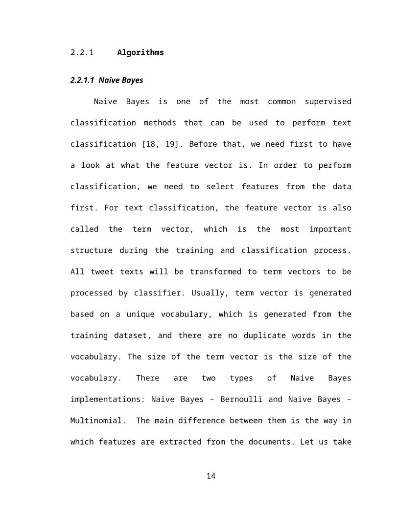
2.2.1.1 Naive Bayes
Naive Bayes is one of the most common supervised classification methods that
can be used to perform text classification [18, 19]. Before that, we need first to have a
look at what the feature vector is. In order to perform classification, we need to select
features from the data first. For text classification, the feature vector is also called the
term vector, which is the most important structure during the training and classification
process. All tweet texts will be transformed to term vectors to be processed by classifier.
Usually, term vector is generated based on a unique vocabulary, which is generated from
the training dataset, and there are no duplicate words in the vocabulary. The size of the
term vector is the size of the vocabulary. There are two types of Naive Bayes
implementations: Naive Bayes – Bernoulli and Naive Bayes – Multinomial. The main
difference between them is the way in which features are extracted from the documents.
Let us take Bernoulli implementation as example, for a sentence like a tweet, a term
vector will initialized with all elements equal to zero. Then check each word in the
vocabulary to see if the word exists in the tweet. If it exists, then mark the corresponding
element in the term vector to 1, if not, mark the corresponding element in the term vector
9

to 0. In that way, if the vocabulary is big enough, every single tweet can be represented
using a term vector with 0s and 1s.
Generally, in text classification, we will ignore the order of words in the
document. Instead, we only consider the presence or absence of the single word, for
instance, whether a word in the vocabulary is included in the document or not. This
model is called a bag of words. It is like we throw all words in a bag and they could be in
any order in the bag.
The element of term vector does not only represent the presence or absence of a
word, it can also represent the frequency of the word.
We can think every term vector as an n-dimension point in an n-dimension
coordinate system, where n is the size of the vocabulary. For the training data, we can
treat it as several classes of a bunch of n-dimension points. Then the text classification
problem becomes traditional points classification problem, though the dimension might
be very large.
For example, if we have a document D, and we have classes C, which contains
some classes. Then in order to get which class that the document D belongs to, we just
need to compute the posterior probability P(C|D), and choose the largest one. P(C|D) can
be computed by Bayes’ Theorem:
P(C∨D)= P ( D|C ) P (C )P ( D )
∝P ( D|C ) P(C )
where the prior probability and likelihood can be computed from the labeled dataset.
Here is how these two algorithms work. Every class is equal probable, so we can
easily get the prior probability P(C ¿¿ i)¿. Let V be the vocabulary, and w j is the j-th
10

word in V, so from the training data, we can get the probability of w j belongs to class C i,
i.e. P(w j∨Ci).
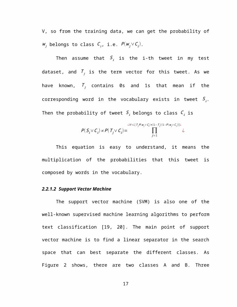
Then assume that Si is the i-th tweet in my test dataset, and T j is the term vector
for this tweet. As we have known, T j contains 0s and 1s that mean if the corresponding
word in the vocabulary exists in tweet Si. Then the probability of tweet Si belongs to class
C i is
P(Si∨Ci)∝P (T j∨C i)= ∏j=1
¿V∨¿[T j P (w j∨C i)+(1−T j)(1−P (w j∨C i))] ¿
¿
This equation is easy to understand, it means the multiplication of the
probabilities that this tweet is composed by words in the vocabulary.
2.2.1.2 Support Vector Machine
The support vector machine (SVM) is also one of the well-known supervised
machine learning algorithms to perform text classification [19, 20]. The main point of
support vector machine is to find a linear separator in the search space that can best
separate the different classes. As Figure 2 shows, there are two classes A and B. Three
hyperplanes between them, I, II and III, separate them into two classes. We will choose
the hyperplane which has the largest normal distance of any of the data points as the best
separator, which is hyperplane I in the following figure.
11

Figure 2: Support Vector Machine on Classification
2.2.1.3 Decision Tree
A decision tree [19, 21] is a simple flowchart that selects labels for input values.
This flowchart consists of decision nodes, which check feature values, and leaf nodes,
which assign labels. To choose the label for an input value, we begin at the flowchart's
initial decision node, known as its root node. This node contains a condition that checks
one of the input value's features, and selects a branch based on that feature's value.
Following the branch that describes our input value, we arrive at a new decision node,
with a new condition on the input value's features. We continue following the branch
selected by each node's condition, until we arrive at a leaf node that provides a label for
the input value.
For the text classification, the decision nodes could be the feature word we
selected, and the leaf nodes could be the categories.
12

2.2.2 Twitter Sentiment Analysis and Stock Price
In the past, public opinions and public sentiment have been suggested and
generally accepted as possible indicators of a company’s stock behavior [24]. In recent
years, there has been an emergence of number of social networks in which a person can
share their emotions, feelings, status or locations, and a surge in their popularity. More
specifically, Twitter has become one of the most important sources of public sentiment
on various topics about companies, products, movies and many others. On Twitter,
although each individual user post, which is called a tweet, is limited to only 140
characters, the millions of tweets could represent public opinions and public sentiment at
a certain extent [25]. Among all their opinions, the opinions of specific companies have
grown in prominence, and it can be argued that Twitter posts by a user are an accurate
representation of a said user’s opinions and thoughts.
It has been discussed that there is a correlation between public opinions and the
stock price [24]. One of the stock price indicators is the market, and customers’ behavior
will have a significant impact on the market. So generally, the public sentiment about a
company and its products is proportion to its stock price behavior. However, little work
has been done to actually expand on this topic. There, for instance, is no time frame as to
how long it takes for a company’s stock to act in accordance to its associated twitter
sentiment, or if there is any demographic on Twitter that does a slightly better job of
predicting a stock’s behavior than another.
13

2.3 Current Distributed Data Processing System
As we mentioned, the MapReduce is not the only solution for Big Data problem.
There are lots of other large-scale data processing solutions and frameworks. Spark [6, 7],
SCOPE [8], Dryad [9] are some other general-purpose systems for large-scale data
processing. Besides the traditional MapReduce, there is a next generation MapReduce
version called YARN in the latest version of Hadoop. In addition, Mesos [10] is a
resource manager for multiple systems including MapReduce, Spark and MPI to share
cluster resources. There are also some frameworks designed for specific computing. For
instance, HaLoop [11] is a MapReduce framework specifically optimized and designed to
perform iterative computing. Pregel [12] is famous for its large-scale graph computing.
Storm [13] is special designed to perform real-time streaming data processing.
2.4 MapReduce Model
MapReduce is a parallel data processing paradigm, which was originally
developed by Google Inc. The MapReduce model contains two phrases, the map phrase
and the reduce phrase. Tuple, which contains a key and a value, is the key data structure
in MapReduce. All data are transferred in tuple structure through the whole process of
MapReduce task. The input to the program is organized in a ¿k1 , v1>¿ pairs. The input
will flow into the map function, and the output format of the map function is a list of
¿k2 , v2>¿ pairs. These outputs will flow into the reduce function, while before that, they
will first be organized by key k 2. Each reduce function will only accepts pairs with the
same key, and a list of values of this key. After these pairs are processed, the output of
14

reduce function will be in the format of ¿k2 , v3>¿ pairs. This process can be presented as
following equations:
map ¿
reduce ¿
In general, there are three stages of a MapReduce task: the splitting stage, the
mapping stage, and the reduction stage. Here we will have an overview of the three
stages in detail.
1. Splitting Stage
When an input dataset comes, the first step is to split it into multiple chunks.
These chunks can be processed in parallel. From the view of this paper [14],
the suggested size of a chunk is equal to the size of the L1 cache available to
the hosting CPU core. Also, there is function called splitter that user can
overwrite to define their own split rules. Usually, this step will be completed
by Hadoop automatically, we do not need to configure a lot for this stage.
2. Mapping Stage
This stage will read the data chunk and partition the data into tuples. Usually,
for a text input file, the input of map function will be every single line in this
file. Through the user defined map function, each line will be processed
individually and emitted in the format of key and value. The outputs of map
functions are the partial results, and these partial results will be shuffled and
sorted by key after they are emitted into the context. We can use our own
defined key_comparator to define the rules of equality of two keys. Also,
15

these shuffled and sorted are called intermediate data and stored in local file
system to be used later in the reduction stage.
3. Reduction Stage
All the aggregation happens in this stage. This stage begins after all map tasks
have completed. Each reduce function will accept a list of values with the
same key. The inputs are from intermediate data. For the list of values, we can
define our own process, and finally, the final outputs of reduce function are
emitted at last. The output is still in tuple format, where the key is the input
key, and the value is usually the aggregation of all the values in the input. All
the output tuples will be written into files in the distributed file system.
This model can be used to apply on large amount of data. The data will be
organized into tuples and passed to map function and reduce function. Both the map
function and reduce function can be run parallel on multiple machines throughout the
cluster.
2.5 An Overview of Hadoop MapReduce Cluster
Hadoop is an open source Big Data framework with the implementation of
MapReduce from Apache software foundation. It is written in Java and it provides us a
high-level programming model for MapReduce. In this section, we will have an overview
of the typical infrastructure of a Hadoop cluster, the Hadoop Distributed File System
[15], and the MapReduce in Hadoop.
16

2.5.1 Hadoop Cluster Infrastructure
Figure 3 shows the typical two level network architecture for a Hadoop cluster.
We can see the cluster is organized into racks. There are typically 30-40 nodes in a rack,
and each rack is connected with a switch to a core switch or router.
In general, there are two kinds of nodes in a Hadoop cluster: the name node (also
called the master node) and the data node (also called worker node). The name node
manages the file system, which is known as Hadoop Distributed File System. The name
node knows the data nodes on which all the blocks for a given file are located. The data
node is the worker of the file system. When a task begins, the data node will find and
retrieve the data from the file system and process the data. The file location is got from
the name node. Also, the data node needs to report back to the name node periodically
with the block locations they are storing.
Figure 3: Hadoop Cluster Infrastructure
17
In general, a Hadoop cluster provides a whole runtime for MapReduce, plus a
distributed file system over the whole cluster.
2.5.2 Hadoop Distributed File System (HDFS)
The Hadoop Distributed File System, also known as HDFS, is another important
feature included in the Hadoop cluster. We have known from the previous part that the
HDFS contains two kinds of nodes: the name node and the data node, and the name node
is to manage the file system, while the data node is to store the data.
In a typical HDFS, the data could be stored on any one of all data nodes, which
means HDFS will divide the data into fixed size blocks, and spread them across all data
nodes in the cluster. Also, Hadoop is designed to run on commodity hardware, there
could be file failures. So each block will be replicated three times, of which two replicas
are placed in the same rack and the other one replica will be in the outside rack. The
name node knows where the blocks are located and tells the location to the data node
once needed.
2.5.3 MapReduce
Hadoop mainly contains two parts: the HDFS and the MapReduce. On the top of
HDFS, the Hadoop MapReduce is the runtime and execution framework for MapReduce
program. The typical Hadoop MapReduce contains two kinds of nodes: a single master
node called JobTracker, and the worker node called TaskTracker. Usually the
TaskTracker runs on the same nodes that HDFS data nodes run on.
18

When a task is assigned or submitted from client, the JobTracker is responsible
for taking it in and assigning TaskTrackers with tasks to be performed. Here we have a
terminology called Data Locality, which means the JobTracker will first try to assign
tasks to the TaskTracker on the data node where the data is locally stored. Otherwise, the
JobTracker will at least try to assign tasks to TaskTrackers within the same rack. In
addition, the JobTracker is responsible for failure tolerance. If a TaskTracker fails, the
JobTracker will detect that and re-assign the task to another TaskTracker. This ensures
the stability of the whole cluster.
TaskTracker runs on each data node and is ready to receive tasks from
JobTracker. In order to let the JobTracker know the running status, the TaskTracker will
send heartbeat to the JobTracker indicating that it is alive. Also, the TaskTracker will
send task running statistics to JobTracker periodically.
Figure 4 shows the relationship between the name node, the data node, the
JobTracker, and the TaskTracker. In summary, a typical data execution flow in Hadoop
cluster is as follows:
(1) The program (also called the client) initializes a MapReduce job and submit it
to the JobTracker;
(2) The JobTracker will get the file location information from the name node, and
try to put the client program in the HDFS. After that, it will try to assign tasks
to TaskTracker based on data locality;
(3) The TaskTracker receives the task and start the mapping phrase. The output of
map function will be stored on local file system as intermediate files. After
19

that, the intermediate results will be passed to reduce function and the final
output of reducing phase is written into HDFS.
(4) After the reducing phase, the job is completed.
Figure 4: Typical Components of a Hadoop Cluster
20
3. NAIVE BAYES FOR TWITTER SENTIMENT ANALYSIS
In this chapter, we will have an overview of the prototype system to find the
correlation between the geographical sentiment on Twitter and the stock price using
Naive Bayes sentiment analysis algorithm, including the data source introduction, the
system methods and implementation, and finally some experimental results.
3.1 Geographical Sentiment and Stock Price
Some researchers have shown that the public sentiment and stock price could be
correlated [24]. The micro blogging site, Twitter, has been used to obtain the public’s
mood for elections [26] and some other particular events, and the idea of using sentiment
found on Twitter and comparing it to a stock’s behavior has been explored. It has been
concluded that there is a strong indication that it may be possible to predict stocks prices
to a certain degree using sentiment analysis. However, location is also an important
aspect of social network, and the location’s sentiment could be an indicator of stock
price’s behavior. Work has not been done on correlating a specific location’s sentiment
affecting a company’s stock behavior.
Twitter doesn’t provide many demographical options, such as gender and
ethnicity. Research has been done to try to find the users’ demographical information [24,
27] by using the user’s self-reported geographic location and seeing if the demographic
information can be accurately represented by Twitter; it was found out that Twitter
sampling that represents 1% of the United States population is biased. No recent papers
on geographical sampling expressed explicitly that sampling was biased [28]. Other work
21

has been done on geographic locations as well, this was a worldwide study and included
geographical locations on user’s offline twitter locations [27]. This section applies the
geographical technique from [28] to obtain locations to locate the most populous cities.
3.2 The Source Data
It was found out that due to the privacy policy of Twitter, public tweets dataset
cannot be obtained. In addition, all the public tweets dataset do not have geographical
information included, which makes it impossible to use the existing datasets.
This system uses Twitter Streaming API to collect the real time data. The input
streaming data is from Twitter’s Streaming API, which is offered by Twitter to give
developers low latency access to Twitter's global stream of Tweet data. We can get all the
global public tweets by passing keywords. The data we receive is in JSON format. Every
tweet is in JSON format including all the information about this tweet. Once connected to
the Streaming API, the data will flow to the system constantly with long connection. The
Twitter Streaming API accepts various filters, for instance, keywords, and languages.
With the keyword filter, the system can only get the tweets about a specific company or
product. The returned data may not have geographical information; in this system only
the tweets with geographical information will be used. With the language filter, only
English tweets are accepted.
The financial data, which is the stock price, is collected from Google Financial
API [29], at 2 minutes intervals.
22

3.3 System Methods and Implementation
This section introduces the methodology and the implementation of the system.
The prototype system will be able to collect tweet data about a specific topic, process the
data, and finally give the geographical sentiment data. Also, the system is designed with
three layers, the data collection layer, the sentiment analysis layer, and the plotting layer.
3.3.1 Three Layer Design
The following figure shows the architecture of the three layer design.
Figure 5: Three-Layer Architecture of the System
The Tweets Collection Layer is to collect the tweets returned by the search query
about a keyword using Twitter Streaming API. The raw data contains a lot of information
but the system only extracts the geographical location information, the tweets body, and
23

the time stamp. For the tweets body, it will be processed by Sentiment Analysis Layer,
which will give a sentiment score based on Naive Bayes approach, and the result will be
sorted by geographical information. At last, the Plotting Layer will plot graphs as needed
for us to do analysis.
3.3.2 Stock Market Sector
A share of stock is literally a share in the ownership of a company. When a person
buys a share of stock, that person is entitled to a small fraction of the assets and earnings
of that company. This means that the more a company earns then that person will invest
in stocks since they hope the company will do well. A source of company earning is from
selling products and services; which is affected by consumer purchases. This means,
however, that the more positive the consumer’s view of a company and its potential
earnings, there may be a higher demand for the stock of said company, and, in turn, the
opportunity to raise the price of a company’s stock is presented. Essentially, this means
that a company’s reputation among consumers can influence its earnings both indirectly
and directly.
The first challenge of our experiment was choosing a company to study; this
company’s stock price and behavior would have had to be tracked and recorded, and later
graphed in order for us to analyze it alongside the graph of its associated Twitter
sentiment.
As the above requirements are somewhat specific, and as there are thousands of
companies trading stock right now, we had to narrow down the search in order to get
more suitable candidates from Standard & Poor’s 500. A specific sector was chosen, and
24

companies falling into that sector were considered. Our sector of choice was food and
restaurants, simply because there was a limited possibility of advertising-related post and
non-relevant posts to be streamed into our dataset, unlike technology companies or TV
companies that have more of an online presence. From previous works, it was very
common to use the Standard & Poor’s 500 to compare stock price and mood or
sentiment, so we decided to draw our companies from that list when deciding which one
we would actually choose.
We selected tweets based on company name keywords, stock ticker symbol, and
uniquely named popular food items for example Frappuccino or Happy Meal. Stock
ticker symbol have been commonly used to search stock related information about a
tweet. We decided to take this into consideration since previous studies have used this
technique. Our goal is to find as many stock related tweets as possible in order to
represent the full sentiment of a company on Twitter.
3.3.3 Geographical Location
As mentioned earlier, there has been some work linking tweets and the stock
market already. It is somewhat accepted in the research community that Twitter, among
other social media sites, can, in some situations, serve as a replacement for the general
public, and polls and questionnaires can now be performed with online media as a
platform. However, because of the relatively new emergence of social media, there is still
much growth for improvement in terms of research, data mining, and a number of other
things.
25

One of our main objectives is finding out whether tweets from one location have a
better correlation to a stock’s price than another, and possibly investigate why. Our
experiment relied on not only taking the general sentiment found on Twitter, but also
dividing this sentiment into different geographical locations. Twitter users have a choice
to report their geographical location on their profile. Locations were collected when
streaming the tweets, and kept a tally on how many tweets each location had. Once all the
streamed tweets were processed, and all of the self-reported locations had a count of the
tweets from users of that location, we simply chose the five states that had the highest
number of tweets. Originally, it was proposed to only filter out tweets from five pre-
specified cities – to be more specific, the five cities that contribute most to the American
GDP – but previous work suggests that Twitter population is not necessarily
representative of the American population, and any of the cities we proposed may not
have had as large of a Twitter presence as we originally thought. In addition, we also
found that if we set the location to a specific city, the amount of tweets we can get is too
small to do some reasonable analysis. Therefore in this system, we expanded the location
box to state.
3.4 Experimental Results
The system has collected all the tweets about Starbucks and McDonald’s for four
days from 9:30AM to 4:00PM EST. In this section, we take Starbucks as an example.
Before that, we will first have an overview of the result representations.
26

3.4.1 Result Representations
The first definition is bullishness score (Bt) for a time period t from paper [30]
given as:
Bt=ln( 1+N postive
1+Nnegative)
In this equation, for each time interval t, the total number of positive tweets is
aggregated as N postive, and the total number of negative tweets is aggregated as N negative. In
this system, this score will be used to plot the graphs.
The expected output is geographical sentiment (bullishness) scores over time
about a specific company or product. The result is sorted by states. The goal of our
system is to track the changes of both geographical sentiment scores and stock prices so
as to find if there is a strong correlation of them. The best way for us to understand the
result would be plot them into some.
The NASDAQ Stock Market operates from 9:30AM to 4:00PM EST. So all the
stock price data and tweets are collected between 9:30AM and 4:00PM EST. This time
period is divided by 10 minutes interval and for each interval in the sentiment graphs, the
bullishness sentiment score is used.
In addition to the plotting, this system also calculates the correlation coefficient in
order to have a measurement of how similar the two graphs are. The correlation
coefficients are calculated based on the following equation:
CORREL( X ,Y )=∑ (x− x)( y− y)
√∑ (x− x)2( y− y )2
27

In this equation, x and y are the sample means of points array X and Y. For the
result, a correlation coefficient of +1 indicates a perfect positive correlation, while a
correlation coefficient of -1 indicates a perfect negative correlation.
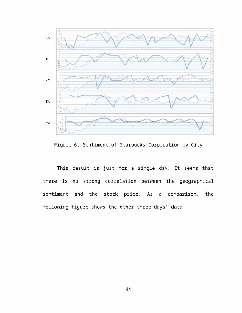
3.4.2 Analysis of the Results
The figure below is the preliminary results for a single day about Starbucks. In the
graph, each of the top five states are above, in the order of California, Illinois, New York,
Texas, and Washington. Each of the above graphs has a timeline of about six and half
hours, divided by 10 minutes interval, and an average sentiment (bullishness) score of
that time period. The graph in the shadow is the stock price line graph from Google
Finance, which is a free service for us to get the historical stock price data and graphs.
Figure 6: Sentiment of Starbucks Corporation by City
28

This result is just for a single day. It seems that there is no strong correlation
between the geographical sentiment and the stock price. As a comparison, the following
figure shows the other three days’ data.
Figure 7: Three Days of Sentiment of Starbucks Corporation by City
In order to have a clear view of their correlations, the following table shows the
correlations coefficients.
Day 1 2 3 4 AVG
CA 0.179 0.138 -0.033 0.127 0.103
IL 0.031 0.442 0.693 -0.027 0.285
NY -0.110 -0.121 0.129 -0.021 -0.031
WA 0.337 -0.184 0.224 -0.365 0.003
TX -0.281 -0.131 0.017 -0.199 -0.149
From the graphs in Figure 6 and Figure 7, it hardly shows correlations between
the shadow lines and the single lines. Sometimes, the two lines may have the same trends,
such as the Washington State in Figure 6, and the first half part of the Illinois State in the
first graph in Figure 7. However this is not always true, the Washington State has a bad
match in the third graph in Figure 7 and the Illinois State also has a bad match in the
29

second graph in Figure 7. In order to know the percentage, or the similarity of the match,
we calculated the correlation coefficients.
From the correlation coefficients table, the New York and the Texas States have
75% negative correlation in all four days, while the other three states in general have a
positive correlation. Also, the Illinois State has the strongest correlation, while the Texas
State has the weakest correlation. This conclusion is about the same as we observed from
the graphs.
Based on what we observed and calculated, we can say that for Starbucks
Corporation, the Illinois State has a strong correlation between the Twitter sentiment and
the stock price. In addition, although the headquarter of the Starbucks is located at
Washington State, the result does not show that the Washington State has a very strong
correlation. In contrast, the Washington State has a very weak but not negative
correlation. In comparison, the Texas State does not have such a strong correlation.
3.5
30

4. NAIVE BAYES MAPREDUCE IMPLEMENTATION
In this chapter, we will introduce the methodologies used and Naive Bayes
MapReduce implementation in this thesis. First, we have an overview of the data
processing methods we used to pre-process input data before it is applied to training
stage. After that, we introduce the parallel implementation of Naive Bayes based
sentiment analysis algorithms in MapReduce. In addition, we review the evaluation
metrics and scenarios used for this thesis.
4.1 Methods Overview
Before we enter into each part, let us have an overview of the whole method, as
the following Figure 8 shows.
As the graph shows, the input data is first pre-processed to remove some noises
that are not useful for sentiment analysis. We implemented a MapReduce system to
perform sentiment analysis based on Naive Bayes classification algorithm in parallel. The
pre-processed data will be fed into the system and ran under different metrics, including
the size of input data, number of nodes, use of global counters, and hardware
configurations. Based on the results, we combine the analysis with some MapReduce
performance factors and try to build the MapReduce performance prediction model.
31

Figure 8: Whole System Method Overview
4.2 Data Pre-processing
We chose Twitter as the source of our data because the Twitter is one of the most
popular social networks in the world. According to Twitter’s IPO filling [22], it has more
than 200 million monthly active users who tweet 500 million tweets per day in 2013.
Another important reason is tweets are almost all about text, while on Facebook or other
social networks the media could be videos, pictures or sharing web links. Twitter allows
people to publish texts with 140 characters limitation. When talking about something,
people intended to talk more specifically and with more feelings or attitudes.
However, Twitter also has some drawbacks. As we know, tweet is not formal text.
Besides the limitation of 140 characters, people also like to use a lot of abbreviations,
32

slangs, emoticons etc. to try to use the least words to express as much feelings as they
can. Also, Twitter allows us to post URL links in the text, to use ‘@’ to refer somebody,
and to use ‘#’ to give tags. This information is not very useful for the sentiment
classification. So the following preprocess is performed to each tweet at the very
beginning.
Figure 9: Tweets Data Pre-processing
1. URLs and ‘@’ Removal
The first step is to remove URLs and the word starts with ‘@’ symbol. We will
not track the content of the web links, so the URLs are deleted. The ‘@’ symbol always
33

has a username followed, which is useless, so the entire word starts with ‘@’ could be
removed.
2. Hashtag Removal
The word starts with ‘#’ is hashtag. Hashtag is different from other words; it gives
a tag, or a topic to the tweet. Usually, the tag is talking about the topic people saying
about in this tweet, not about people’s attitudes. This word might provide some
information but not that important. So I decided not to remove the entire word, but to just
remove the ‘#’ symbol, and treat the tag as a normal word in tweet.
3. Punctuations Removal
We do not need punctuations as the features, they are just symbols to separate
sentences and words, so they should be removed.
4. Stopwords Removal
There is a kind of word called stopword [24]. They are some common function
words in a sentence, like ‘a’, ‘the’, ‘and’, ‘to’, ‘at’, etc. These words seem to be useless
for sentiment analysis, and also these words appears a lot of time in English, if we use
term frequency to determine if a word is informative, these words will account for a large
proportion. So these words should be removed.
5. Digital words Removal
Some words start with a digit, like ‘1990’, ‘4:00pm’ etc. These words also have
no relationship with attitudes or feelings. So these words should be removed.
After the pre-process of dataset, all tweets will only have some plain words.
Through this pre-process, noises are removed so that we can build better vocabulary and
have smaller dimension of the term vector.
34

4.3 Parallel Naive Bayes in MapReduce
We have already introduced the sequential Naive Bayes algorithms for text
classification based sentiment analysis algorithms in chapter 2. MapReduce is another
new parallel programming model so that we need to adjust these algorithms to fit into
MapReduce model. In this section, we will introduce the parallel implementations of
Naive Bayes based sentiment analysis algorithm in MapReduce model.
4.3.1 Algorithm Implementation
Let us first have a look at the equation of Naive Bayes for sentiment
classification.
P(C∨D)= P ( D|C ) P (C )P ( D )
∝P ( D|C ) P(C )
We can see from the equation that the most two important values we need to
compute the posterior probabilities are class prior probabilities P(C) and likelihoods
P ( D|C ). For a training set, it seems that in order to get these two values, we need to have
some counts. Here we use C to refer to the label of the tweet, and X to refer the features
(words). What we needs are:
1. Number of tweets: the number of all tweets.
2. Number of C: the number of unique labels.
3. Number of C = c: the number of tweets with label c. This should be a global
variable and can be used with the previous number we have to compute label
prior probabilities.
4. Number of X in C = c: the number of words that are in all the tweets with
label c.
35

5. Number of X = x in C = c: the number of word x that is in all the tweets with
label c. This number and the previous number we have are combined to
compute the probabilities of a single word x under a label c.
6. |V|: the total number of unique words in all tweets. This is actually the size of
our vocabulary.
Using the above data, we can get the prior probabilities P(C) and likelihoods
P ( D|C ).
It is obvious that only one mapper and reducer job is not enough. And our goal is
to build the prediction model, which means we only need to test the training phase. In
general there are two jobs: the word job and the label job. For each job there is a map
function and a reduce function. The word job is to compute the likelihood of each word,
and the label job is to compute the prior probability of each label. Let us take a look at
each job in details.
1. The Word Job
This job is mainly about word counting. The reason we call it Word job is
because this job will output all the statistics about every single word. As we
know, the job will have a map function and a reduce function, and each function
takes tuples. Here are the inputs and outputs of these two functions.
WordMapper
Input: each line (tweet) of the text
Output: <word, label>
Algorithm:
36

map(docID, line):
label = line[0]
text = pre_processing(line[1:])
textArray = text.split(‘ ’)
for word in textArray:
emit(word, label)
The mapper will receive every single line of tweet in the input dataset.
The line contains two parts, the first part is the label, and the second part is the
tweet body. For the tweet body, we invoke a function called pre_processing()
to perform pre-processing on the tweet as we mentioned earlier in this thesis
before. We use two variables to store these two values: label and text. Then
the pre-processed tweet will be split into every single word delimitated by
space and stored in the variable textArray. Then we put every word and its
label into a tuple and emit it to the context. For example, we have a tweet with
label “positive”:
“positive I like the weather today :)”
After pre-processing we can get:
“positive like weather today”
Then the output of the mapper will be three tuples:
“<like, positive>”
“<weather, positive>”
“<today, positive>”
37

These outputs will be passed to the WordReducer.
WordReducer
Input: <word, label>
Output: <word, label_1:count label_2:count ... label_n:count>
Algorithm:
reduce(word, label[]):
|V|++
HashMap labelCounts;
for label in label[]:
if labelCounts has key label:
labelCounts[label]++
else:
labelCounts[label] = 1
for key, value in labelCounts:
output += “key:value”
emit(word, output)
During the shuffle and sort process, the output tuples from the
WordMapper will be sorted by the key word. All the labels with the same key
word will be passed into one reducer as an array. For example, we have these
three values from the mapper:
<like, negative>
<like, positive>
38

<like, positive>
Then they will be re-organized as one tuple:
<like, [negative, positive, positive]>
In the reducer, because all the tuples with the same key word will be
passed only to one reducer, so the first step is to add one to a global variable
V, which is the size of vocabulary. This variable will have the count of all
unique word in the corpus at last. Then for the label array, we use a HashMap
to count every label. The HashMap will be defined as follows:
HashMap<String, Integer>
The key of the map is the label string, and the value with key is an
integer number storing the count of the label. If the label is already in the
HashMap, the value will be added by one, otherwise a new key associated
with the label will be created.
At last, the key and value pairs will be put into an output string and
emitted by the reducer with the word. For example, the output of the previous
input will be:
<like, negative:1 positive 2>
Until now, the whole Word Job is finished. The output of the reducer
will be written into a temporary file in HDFS and this file will be used later to
get all statistics about training model.
2. The Label Job
39

This job is mainly about label counts. The reason we call it Label Job
is because this job will generate some label statistics. Let us take a look at the
mapper and reducer function.
LabelMapper
Input: each line (tweet) of the text
Output: <label, word_count>
Algorithm:
map(docID, line):
label = line[0]
text = pre_processing(line[1:])
textArray = text.split(‘ ’)
emit(label, textArray.length)
The mapper will receive every single tweet as input. After pre-
processing of the tweet, and split by space, we can get an array of the
words in that tweet. In this mapper, we simply emit the word number
along with the label. For example, if the input tweet is this:
“positive I like the weather today :)”
After pre-processing we can get:
“positive like weather today”
Then the output of the mapper will be a tuple:
<positive, 3>
40

This tuple means, this tweet is positive and it has 3 valid words or
features. The output will be written into intermediate files and passed into
the LabelReducer.
LabelReducer
Input: <label, word_count>
Output: <label, tweet_number:word_number>
Algorithm:
reduce(label, int[]):
UniqueLabelNumber++
for count in int[]:
docNumWithLabelY++
wordNumWithLabelY += count
emit(label, docNumWithLabelY:wordNumWithLabelY)
The reducer will take all the word counts associated with the same
label as input. The input is also re-organized by shuffle and sort process
before passed into the reducer. In the reducer, there is another global
variable named UniqueLabelNumber, which is the number of all unique
labels, because each reducer will only accept one kind of label. Then for
the word count array, we will iterate over each element and add the value
to a variable wordNumWithLabelY, which is the number of all words in
the tweets with label Y (the label Y here is just an example). At the same
41

time, another variable docNumWithLabelY will be added by one to
calculate the number of tweet with label Y.
At last, the variable docNumWithLabelY and wordNumWithLabelY
will be combined together and emitted out along with the label. For
example, if the output is:
<positive, 12:514>
This tuple means there are 12 tweets that are belonged to positive category
and of all that tweets there are 514 words totally. These results will be
written into HDFS and used later.
Until now, let us have a look at what data we can generate from these two jobs. In
this example, we take word “happy” as a feature word.
(happy, positive:3 negative:1)
3 positive tweets having word ‘happy’, 1 negative tweet having word ‘happy’.
(positive, 6:20)
6 positive tweets with 20 words totally.
(negative, 5:16)
5 negative tweets with 16 words totally.
|V| = 25
The vocabulary size, 25 unique words in all the tweets.
From the data above, let us see what we can get.
Prior probabilities:
P( positive)= 65+6
42

P(negative )= 55+6
Likelihoods (with Laplacian Smoothing):
P (happy|positive )= 3+16+25
= 431
P (happy|¬ative )= 1+15+25
= 115
After we get the prior probabilities and likelihoods, if we have a new tweet to be
classified, we can simply apply the equation:
P(C∨D)= P ( D|C ) P (C )P ( D )
∝P ( D|C ) P(C )
to get the posterior probabilities:
P ( p ositive|new tweet )∝P (positive)∏ P(wordn∨positive)
P (negative|newtweet )∝P(negative)∏ P(word n∨negative)
Then we select the category with a higher prediction rate as the result of our
classification.
4.3.2 Algorithm Time Complexity
The time complexity of Naive Bayes based sentiment analysis algorithm is mainly
determined by two processes: the computation of prior probabilities of classes, and the
computation of likelihoods of feature each word P(wt∨C j). Let us assume that there are
c classes, and the number of feature words, which is the size of vocabulary, is |V|. Then
we can get:
(1) Computing the prior probabilities of each class: O(c )
(2) Computing the term frequency of each feature word: O ¿
43

(3) Counting the number of documents/tweets: O(1)
(4) Computing the likelihoods of each feature word: O ¿
In total, the time complexity of Naive Bayes based classification MapReduce
algorithm on a single node is:
T (n )=O (c )+O¿
Assume that we have n nodes, and then the computation will be distributed to n
nodes. So the time complexity of the parallel MapReduce Naive Bayes sentiment analysis
algorithm on n nodes cluster will be:
T (n )=O ¿¿
From the equation, we can see that the time complexity will be decreased while
the number of nodes increases.
4.3.3
44

5. EXPERIMENTAL RESULTS
In this chapter, we will introduce some metrics we used in this thesis to test the
performance, and the testing scenarios including out datasets and hardware configuration.
We will analyze the testing results regarding to the relationship between the execution
time and number of nodes, the input data size, the use of global counters, and the
hardware configuration.
5.1 Metrics Summary
In order to have an overview of the execution status of a MapReduce job, we need
to define some metrics to observe during the job execution. In this thesis, what we call
the performance is actually defined by the time of execution. The shorter the execution
time is, the better the performance is. There are a lot of other aspects that can affect the
execution time, such as the number of nodes, the size of the input dataset, or the use of
global counters in a MapReduce job, etc. So we need to change these metrics during the
execution of the job and observe the changes of the results.
5.1.1 Terminologies
For a MapReduce job, we will first define some terminologies we used in this
thesis.
(1) Total Execution Time
This is the time consumed during the whole job, which means it is counted
from the point of job starting and to the point of job ending, including
everything happened in the job.
45

(2) Total Slot Execution Time
This is a little different from the total execution time because this slot
execution time is only about the time consumed by the mapper and reducer
execution. This time is usually shorter than the total execution time, the
difference is mainly about I/O transferring time, the network communication,
and job scheduling time, etc.
(3) CPU Time
This is a little harder to understand, because this time will not change if a job
does not change. This is the time consumed by CPU, which is used for
processing instructions of a computer program. It is only related to the number
of instructions in a program, which means if we parallelize a program, the
total execution time might be the third of the original, but the CPU time would
not change because the amount of instructions does not change but are
executed in parallel.
(4) Global Counters
Hadoop framework does not have global variable sharing mechanism, while it
provides a global counter mechanism. From the name we can know that it is
mainly for counting. We may need to keep track of some counters like how
often a certain event has occurred during the job execution. Because of this
feature of global counter, we can use it to share some global values during the
whole job, such as how many documents or tweets in total, how many unique
words in total. Global counters are reported back to the job tracker from the
task tracker repeatedly like heart beating.
46

5.1.2 Impact of Node Number
For a cluster, the number of nodes is one of the very important aspects that affect
the whole performance of execution. As we introduced in the time complexity section,
the time complexity and the number of nodes is inversely proportional. However we do
not know the exact relationship between them. Therefore, the number of nodes is one of
many metrics we will evaluate in this thesis.
5.1.3 Impact of Data Size
The data is the key to the program, and it directly affects the execution time
because the program is to process data. It is obvious that in a sequential algorithm, the
execution time should be linear to the size of data. However, in Hadoop cluster, the data
is distributed and stored in Hadoop Distributed File System. There might be many other
aspects that affect the relationship between the data size and the execution time. It is a
cluster with many nodes, data may need to be transferred or re-organized at anytime. Plus
the locality feature of Hadoop framework, the impact of data size still needs to be
observed and analyzed.
5.1.4 Impact of Global Counters
In common programming practice, the global variables are usually avoided to use
because they could bring a lot of sharing or synchronization problems. The global
variable needs to be synchronized to avoid mutual operations. Also, the global variable
will be allocated in shared memory, and any inappropriate operations would cause
unknown problems. Usually, it is impossible to share global variables between nodes in a
large cluster, or it will cost a lot of I/O and affect the performance of the program
47
seriously. Although Hadoop provides us a new mechanism to count some events across
the whole cluster, we still need to know how costly it is during a MapReduce job
execution.
5.2 Evaluation Scenarios
In this section, we will have an overview of the format of the dataset used in this
thesis, and the hardware configuration, which is the Hadoop environment.
5.2.1 Dataset
The dataset we used in this thesis is in CSV format. In the data file, each line is a
single input including two parts: the label and the body of the tweet. There are two
categories in our dataset, positive and negative. We used number 0 to represent negative
and number 4 to represent positive. Here is a snippet of the dataset:
0, I forgot my phone in my car but I'm too scared to go outside and get it.0, feels like crying, that's how sick I feel!!4, The SUN is shining!! I'm happy :)4, @hype6477 Good to hear all's cool. I've just sent you a DM hope it'll start to help you
As we can see from the snippet, there are two kinds of tweets: 0 for negative and
4 for positive. The tweet body in the second column is the original one with
abbreviations, emoticons, or ‘@’ symbol etc. in it. The size of dataset we used in this
thesis is 0.25GB, 0.5GB, 1GB, 2GB, and 4GB.
5.2.2 Hardware Configuration
We used Amazon Elastic MapReduce (EMR) [23] as the experiment
environment. As the official states, Amazon Elastic MapReduce is a web service that
48

makes it easy to quickly and cost-effectively process vast amounts of data. We can create
a Hadoop cluster with different node types and applications (Hive, HBase, etc.) on the
cloud. We can create any number of nodes in the cluster, and after that, there is SSH
access to the master node. Using the SSH connection, we can upload our jar files, data
files, execute Hadoop programs, or install our own dependencies on the master node.
After the job is done, the EMR cluster can be terminated so that the computation
resources can be assigned to others.
Besides the Amazon EMR service, there is another service called Amazon Simple
Storage Service (S3) to provide secure, durable, highly scalable object storage. The
advantage of Amazon S3 is that it can be used along with other Amazon Web Services,
such as Amazon EMR. Although we can use SSH to connect to the master node and
upload our dataset, this is not a very efficient way. If the dataset is very large, it will take
a lot of time to be uploaded and we still need to put it into HDFS after it is uploaded to
the local file system on the master node. Once the cluster is terminated, the data we
uploaded will be erased permanently. Using S3 can solve all these inconveniences. S3
can be used directly in Amazon EMR as HDFS, which means, we can upload data files to
S3 and we can get an URL to this file. This URL can be treated as an HDFS URL and
shared by multiple nodes. In this case, the data will not be lost and the size of the data
could be very large. The basic infrastructure of Amazon EMR is shown in the following
figure.
49

Figure 10: Basic Amazon EMR Infrastructure
In this thesis, the Hadoop cluster was created on Amazon EMR, and the data was
uploaded to S3. There are several different kinds of nodes provided by Amazon EMR,
and we used the M1 large type, with the following hardware configuration:
Model vCPU Memory (GiB) Storage (GB)
M1 large 2 7.5 2 x 420
As comparison, we also used the M2 4xlarge type, with the following hardware
configuration:
Model vCPU Memory (GiB) Storage (GB)
M2 4xlarge 8 68.4 4 x 420
All these features and configurations make it a perfect choice for a Hadoop
cluster. As for the number of nodes, we created several clusters with 1, 2, 4, 6 and 8
nodes, respectively to run different sizes of data and collect the results.
50

In the following part, we will demonstrate the running results of parallel
MapReduce Naive Bayes based sentiment analysis algorithm on different sizes of data
input with different clusters and configurations. Each metric will have visualized graphs
and corresponding analysis.
To classify, the data sizes are 0.25GB, 0.5GB, 1GB, 2GB, and 4GB respectively
and the numbers of nodes are 1, 2, 4, 6 and 8 respectively.
5.3 CPU Time
In this experiment, we used M1 large type of node. As we introduced before, the
CPU time is the time consumed by instructions. For a specific job, if the size of data to be
processed and the program itself are constant, the number of instructions that will be
executed in CPU is constant. Therefore, for each input size, the CPU execution time
should be constant no matter how many nodes are used for the job. The results are plotted
in Figure 11 below.
In Figure 11, the vertical axis is the CPU execution time and the unit is minute.
The horizontal axis is the number of nodes. The legend is the size of input data. There are
five serious in this figure, and each color represents a size of the input data. As we can
see from the figure, if the input size is constant, the CPU execution time is constant as
well, no matter how many nodes are used. This result verifies our hypothesis for CPU
execution time.
From the result above, we conclude that the instructions executed in a job will not
change. If the total time or total slot time changes later, then they must be affected by
other aspects. This conclusion is the foundation of later hypothesis and analysis.
51

1 node 2 node 4 node 6 node 8 node0
20
40
60
80
100
120
140
0.250.5124
Number of nodes
CP
U T
ime
(min
)
Figure 11: CPU Time and Number of Nodes
There is another important hypothesis that the amount of instructions executed by
CPU should be proportional to the input data size because the main computing is about
data processing. The following Figure 12 shows the relationship between the CPU time
and the size of input data.
In Figure 12, the vertical axis is the CPU execution time and the unit is minute.
The horizontal axis is the size the input data. The legend is the number of nodes. We can
see that the five lines overlap because the CPU time is not affected by the number of
nodes. And what the most important is the CPU time and the size of input data are
linearly related, which verifies the hypothesis we made before is correct.
52

0.25 0.5 0.75 1 1.25 1.5 1.75 2 2.25 2.5 2.75 3 3.25 3.5 3.75 40
20
40
60
80
100
120
140
1 node2 node4 node6 node8 node
Size of data (GB)
CP
U T
ime
(min
)
Figure 12: CPU Time and Size of Data
From the above analysis, let us try to find the function to define the relationship
between the CPU time and the number of nodes, size of input data. First, let us define
some variables. These variables will also be used in the later analysis. Use variable n to
define the number of nodes in a cluster. Use variable s to define the size of the input data.
For the CPU time, from the figures and analysis above, we define a function y1 to
represent the relationship. We have known that the CPU time has no relationship with the
number of nodes, and is linearly proportional to the size of input data, therefore the
function can be written as:
y1=f (s )=a ∙ s+b
In the equation, variables a and b are two coefficients.
5.4 Data Size
In this experiment, we still used M1 large type of node. We have introduced two
terminologies before: the total execution time, and the total slot execution time. For this
53

experiment, we will run the job with different size of input data on multiple clusters with
different number of nodes, and try to find the relationship between the time and the data
size. In addition, the difference between the total execution time and the total slot
execution time could be the time consumed by I/O, and scheduling. We will also have a
brief analysis on this time.
5.4.1 Total Execution Time
The total execution time is collected by the program itself. The experiment results
are plotted in Figure 13 below.
0.25 0.5 0.75 1 1.25 1.5 1.75 2 2.25 2.5 2.75 3 3.25 3.5 3.75 40
10
20
30
40
50
60
70
1 node2 node4 node6 node8 node
Size of dataset (GB)
Tot
al E
xecu
tion
Tim
e (m
in)
Figure 13: The Total Execution Time and Size of Data
In Figure 13 above, the vertical axis is the total execution time and the unit is
minute. The horizontal axis is the size the input data. The legend is the number of nodes.
From the above Figure, we can get the following conclusions:
54

(1) For each node number, the total execution time is linearly related to the
size of input data.
This result proves that the MapReduce parallelization does not change the
linear relationship between the execution time and the input data size.
(2) The total execution times of 1 node and 2 nodes cluster are the same.
According to our previous analysis, when the number of nodes increases, the
total execution time would decrease linearly. However this is not true for the
case where the number of nodes increases to 2 from 1. The reason is that when
we only had 1 node, this node will serve as both the master node and worker
node. Actually it is mainly about worker node because the main computation
is consumed by data processing on worker node. However, when we increases
the number of nodes to 2, one of them will serve as master node and the other
one will serve as the worker node, so actually, there is still only one worker
node to process the data. These two cases are almost the same. That is why
when the number of nodes increases from 1 to 2 does not have any significant
affects on the total execution time.
This is always true for the future situations, that we can see the 1 node cluster
and 2 nodes cluster would not have significant differences.
(3) The execution time decreases while the number of nodes increases.
This relationship seems not to be linearly. We will talk more about this in the
next section about number of nodes.
55

5.4.2 Total Slot Execution Time
From the previous section, we have known that the total execution is linearly
related to the input data size. However, the total execution time includes many other time
consumed in the job, such as the I/O time, and the scheduling time. These times may or
may not be proportional to the input data size, or linearly related. Since we have had all
the slot times, the differences between them are the time for this part.
First, let us have an overview of the relationship between the total slot execution
time and the input data size. It is expected to be linearly related and almost the same as
the total execution time relationship. The results are plotted in the following Figure 14:
0.25 0.5 0.75 1 1.25 1.5 1.75 2 2.25 2.5 2.75 3 3.25 3.5 3.75 40
10
20
30
40
50
60
70
1 node2 node4 node6 node8 node
Size of input data (GB)
Tot
al s
lot e
xecu
tion
tim
e (m
in)
Figure 14: The Total Slot Time and Size of Input Data
In Figure 14 above, the vertical axis is the total slot execution time and the unit is
minute. The horizontal axis is the size the input data. The legend is the number of nodes.
56

From the above Figure, we can get all the same conclusions as the relationship between
total execution time and the size of input data in the previous results.
Then let us have a look at the relationship between the differences and the input
data size, as Figure 15 shows below.
0.25 0.5 0.75 1 1.25 1.5 1.75 2 2.25 2.5 2.75 3 3.25 3.5 3.75 40
2
4
6
8
10
12
14
1 node2 node4 node6 node8 node
Size of input data (GB)
Diff
eren
ces T
ime
(min
)
Figure 15: The Difference Time and Size of Input Data
In the above Figure 15, the vertical axis is the difference time between the total
execution time and total slot execution time, and the unit is minute. The horizontal axis is
the size of input data. The legend is the number of nodes. From the above Figure, we can
get the following conclusions:
(1) For the 1 node and 2 nodes cluster, the difference time stays stable
without any changes.
57

We have talked about the reason for this phenomenon in the previous section,
that the 1 node cluster and 2 nodes cluster do not have significant differences
because there is always only 1 worker node in these two clusters. Due to the
data locality policy, there would be no data transferred between nodes, which
means not too much I/O cost, and the scheduling would be only for a single
worker node, which makes it easier and not cost too much time.
(2) The difference time starts to increase after the input data is bigger than
0.5GB, and they are linearly related.
As we mentioned before, this difference time including the I/O time, and the
scheduling time, etc. When the data is too small, the I/O cost between nodes
might be constant. While when the data size is beyond a value, this I/O cost
cannot be ignored any more because it means more data needs to be
transferred between nodes and the difference time increases. It is good to see
that the relationship is kind of linear, which means the data allocation is well
balanced in Hadoop.
From all the above analysis, let us try to find the function to define the
relationship between the total execution time and the size of input data. We still use
variable s to define the size of the input data. From the figures and analysis above, we
define a function g(s) to represent the relationship. We have known that total execution
time is linearly proportional to the size of input data; therefore the function can be written
as:
g (s )=c ∙ s+d
In the equation, variables c and d are two coefficients.
58

5.5 Number of Nodes
In the previous section, we analyzed the relationship between the execution time
and the input data size. In this experiment, we will try to analyze the results we get to find
the relationship between execution time and the number of nodes in the cluster. We still
used M1 large type of node, and run the job with different size of input data on multiple
clusters with different number of nodes. We will analyze the relationship between the
number of nodes and the total execution time, total slot execution time, and the speedup.
5.5.1 Total Execution Time
In this section we will analyze the relationship between the total execution time
and the number of nodes. The results are plotted in the following Figure 16:
1 node 2 node 3 node 4 node 5 node 6 node 7 node 8 node0
10
20
30
40
50
60
70
0.250.5124
Number of nodes
Tot
al E
xecu
tion
Tim
e (m
in)
Figure 16: The Total Execution Time and The Number of Nodes
59

In the above Figure 16, the vertical axis is the total execution time, and the unit is
minute. The horizontal axis is the number of nodes. The legend is the input size, and the
unit is GB. From the above Figure, we can get the following conclusions:
(1) The total execution time stays the same when the number of node
increases from 1 to 2.
We have observed and analyzed this phenomenon in the pervious sections.
The reason is that for both 1 node cluster and 2 nodes cluster, there is always
only 1 worker node, so the total execution time will not change.
(2) After the number of nodes is beyond 2, the relationship between the total
execution time and the number of nodes seems to be inverse proportion.
From the previous chapter of time complexity, we had the conclusion that if
we have n nodes in the cluster, the time complexity of the parallel MapReduce
Naive Bayes based sentiment analysis algorithm would be:
T (n )=O ¿¿
In this equation, c is the number of classes and |V| is the size of feature words.
From this equation, we can have a hypothesis that the total execution time
should be inverse proportional to the number of nodes. The results in Figure
16 prove that this hypothesis is correct when the number of nodes increases
from 2 to 8. And also, the bigger the input data size is, the bigger the size of |
V| is, so the graph in Figure 16 is more gently. This experiment results also
prove that the previous time complexity analysis is correct.
60

5.5.2 Total Slot Execution Time
The experiment results for this section are plotted in the following Figure 17.
In Figure 17, the vertical axis is the total slot execution time and the unit is
minute. The horizontal axis is the number of nodes. The legend is the size of input data,
and the unit is GB. From the Figure, we can get all the same conclusions as the
relationship between total execution time and the number of nodes in the previous
discussion.
1 node 2 node 3 node 4 node 5 node 6 node 7 node 8 node0
10
20
30
40
50
60
70
0.250.5124
Number of nodes
Tot
al S
lot E
xecu
tion
Tim
e (m
in)
Figure 17: The Total Slot Execution Time and The Number of Nodes
From the above analysis, let us try to find the function to define the relationship
between the total execution time and the number of nodes. We still use variable n to
define the number of nodes. From the figures and the algorithm analysis above, we define
a function q (n) to represent the relationship. We have known that total execution time is
61

inversely proportional to the size of number of nodes; therefore the function can be
written as:
q ( n )= en+ f
In the equation, variables e and f are two coefficients.
Let us define a new function y2 to represent the relationship between the total
execution time and the number of nodes, size of data. Then we can get:
y2=g ( s ) ∙ q (n )= (c ∙ s+d ) ∙( en+ f )
¿ ce ∙ sn
+cf ∙ s+ den
+df
In the equation, variables c, d, e, and f are coefficients. We can use some constant
variables to replace them. If the number of nodes is fixed, then the relationship between
the total execution time and the size of input data is:
y2=A ∙ s+B
This equation means the total execution time and the size of input data is linearly
related. If the size of input data is fixed, then the relationship between the total execution
time and the number of nodes is:
y2=A'
n+B'
This equation means the total execution time and the number of nodes is inversely
related.
In addition, just as the discussion in the previous section, the relationship between
the difference time and the size of input data, here we will have a look at the relationship
62

between the difference time and the number of node. The result is plotted in the following
Figure 18.
1 node 2 node 3 node 4 node 5 node 6 node 7 node 8 node0
2
4
6
8
10
12
14
0.250.5124
Size of input data
Diffe
renc
es T
ime
(min
)
Figure 18: The Difference Time and Size of Input Data
In the above Figure 18, the vertical axis is the difference time between the total
execution time and total slot execution time, and the unit is minute. The horizontal axis is
the size of input data. The legend is the number of nodes. From the above Figure, we can
get the following conclusions:
(1) For the 1 node and 2 nodes cluster, the difference time stays stable no
matter how input size changes.
We have talked about the reason for this phenomenon in the previous section,
that the 1 node cluster and 2 nodes cluster do not have significant differences
because there is always only 1 worker node in these two clusters. Due to the
data locality policy, there would be no data transferred between nodes, which
63

means not too much I/O cost, and the scheduling would be only for a single
worker node, which makes it easier and not cost too much time.
(2) When the number of node is 4, it gives the biggest difference time, which
means the worst performance. After 4 nodes, the difference time
converges to balances status.
Through the experiments, we figured out that for the input data size is bigger
than 1GB, the difference time would have a peak point when the number of
node is 4. After that, the difference time will decrease and converges to a
constant value. We do not have data for 3 nodes, but the difference time
would be high as well when number of node is 3, because when the number
of worker nodes increases from 1 (the number of nodes is 2), data stored in
HDFS should be duplicated to ensure the stability. The default duplication
number of data in Hadoop is 3, so when the number of nodes reaches 4,
which means the number of worker node is 3, the data duplication reaches
the peak. Data should be transferred in the network 3 times and that will cost
a lot of I/O communication. After that, when the number of nodes increases,
the data duplication will be distributed over the whole cluster, and finally it
will get a balanced status, which is why the difference time would converge
to a constant value as the number of nodes increases.
5.5.3 Speedup
The reason why we studied the speedup is to verify the relationships we found
before are correct. First, let us define the speedup here. For each job, we have a CPU
64

time, which can be treated as the ground truth or the sequential time. Also, we have a
total execution time, which usually is faster than the CPU time because it is executed in
parallel MapReduce model. If we want to know how fast the parallelization can perform,
we define a speedup variable like this:
Speedup= CPU timeTotal executiontime
Before the analysis, let us have a look at the results we got from our experiments.
The results are plotted in the following Figure 19.
0.25 0.5 0.75 1 1.25 1.5 1.75 2 2.25 2.5 2.75 3 3.25 3.5 3.75 40
1
2
3
4
5
6
7
8
9
10
1 node2 node4 node6 node8 node
Size of data (GB)
Spee
dup
Figure 19: Speedup and Size of Data
65

1 node 2 node 4 node 6 node 8 node0
1
2
3
4
5
6
7
8
9
10
0.250.5124
Number of nodes
Spee
dup
Figure 20: Speedup and The Number of Nodes
We can observe from Figure 20 that the speedup does not change when the
number of nodes increases from 1 to 2, which is the same as we analyzed before. While,
later as the size of input data and the number of nodes increase, the speedup increases as
well. In order to find the relationship, let us use the relationship functions we found
before.
We define a function y3 to represent the relationship between the speedup and the
number of nodes, size of data. We have function y1 to represent the CPU time
relationship, and function y2 to represent the total execution time relationship, then we
can get the equation:
y3=y1
y2= a ∙ s+b
ce ∙ sn
+cf ∙ s+ den
+df
66

In the equation, variables a, b, c, d, e, and f are coefficients. We can use some
constant variables to replace them. If the number of nodes n is fixed, then the relationship
between the speedup and the size of input data s is:
y3=A ∙ s+BC ∙s+D
=A+ B
s
C+ Ds
This equation means the speedup is proportional to the size of data s, but not
linearly related. And when the size of input s is too large, the speedup would be stable
and approach to a constant value. If the size of input data s is fixed, then the relationship
between the speedup and the number of nodes n is:
y3=A '
B'
n+C'
This equation means the speedup is also proportional to the number of nodes n,
but not linearly related. And when the number of nodes n is too large, the speedup would
also be stable and converge to a constant value.
5.6 Hardware Configuration
In addition to the size of input data and the number of nodes in a cluster, the
hardware configuration could also affect the performance a MapReduce program. In our
experiment, there are two types of nodes, the M1 large, and the M2 4xlarge. Here are the
configurations:
Model vCPU Memory (GiB) Storage (GB)
M1 large 2 7.5 2 x 420
M2 4xlarge 8 68.4 4 x 420
67

We run our program on two 8 nodes cluster with these two kinds of nodes in each
cluster. The size of input data is the same as previous experiments.
0.25 0.5 0.75 1 1.25 1.5 1.75 2 2.25 2.5 2.75 3 3.25 3.5 3.75 40
1
2
3
4
5
6
7
M1 largeM2 4xlarge
Size of data (GB)
Tot
al e
xecu
tion
time
(min
)
Figure 21: Total Execution Time and Size of Data From Two Clusters
As we can see from the above figure, the larger and more powerful machine can
bring some performance improvements. The Amazon Web Service calls the larger node
4xlarge, it means on the whole point the 4xlarge node is 4 times better than the large one.
However, from the results we got in Figure 21, the performance improvement is not
always exactly 4 times. To some extent, upgrading the hardware can bring performance
improvements, but in reality, we still need to make this decision carefully because
upgrading hardware of a cluster is hard, and will cost a lot.
68

5.7 Global Counters
It is hard to share global values in a distributed system. Even if we can, it would
give us a lot of problems like the synchronization. However, in MapReduce programming
model, sometimes we need to share some variables or collect some data from each
mapper or reducer. Hadoop provides us a mechanism called global counters to collect
count data from each node. We have talked about the details about global counters in the
previous section. Although global counter is well implemented in Hadoop, it still
consumes some resources. We also want to find out how the global variables will affect
the performance of our parallel MapReduce Naive Bayes based sentiment analysis
algorithm.
As the previous part introduced, there are two user defined global counter in our
algorithm, the size of vocabulary, and the unique label number. As comparison, we
removed these two global counters and used constant values. The experiment was
conducted on 6 nodes cluster with M1 large type of node. The input data is the same as
we used before. The total execution time was used to evaluate the performance. The
results are plotted in the following Figure 22.
69

0.250.50.75 1 1.251.51.75 2 2.252.52.75 3 3.253.53.75 40
2
4
6
8
10
12
14
16
18
With CountersWithout Counters
Size of data (GB)
Tot
al e
xecu
tion
time
(min
)
Figure 22: The Total Time Execution and The Size of Data About Counters
As we can see from the Figure 22Figure 22: The Total Time Execution and The
Size of Data About Counters, the differences caused by global counters are very small
and can be ignored. If we do not use global counters, we need to use other ways to share
values, such as writing to a file, which would less efficient than the global counter itself.
The conclusion is that use global counters as needed and it would not affect the whole
performance of the program very much.
70

6. CONCLUSION
Text classification is one of the most important areas in text data mining, and
sentiment analysis can be performed based on text classification. While the data is
exploded today, it becomes a problem to classify large amount of data. The MapReduce
programming model solves this problem by providing a mechanism to manage and
process data over the cluster.
Naive Bayes is one of the algorithms to perform sentiment analysis. The general
idea is to do some word counting and compute some statistics data to build the classifier.
A prototype system to find the correlations between geographical Twitter sentiment and
stock price using Naive Bayes has been implemented. Through this system, we can
collect and analyze the sentiment of tweets based on geographical information, and try to
find the correlation between the geographical sentiment and the stock prices of
companies. The preliminary results show that for the Starbucks Corporation, there is a
week correlation between them, and among the five the states the Illinois State has the
strongest correlation, while the Texas State has the weakest correlation.
The Naive Bayes sentiment analysis algorithm has also been proved to be suitable
for MapReduce programming model. Based on Hadoop framework, we implemented the
parallel Naive Bayes based sentiment analysis algorithm in MapReduce model, and
through a series of experiments and analysis, the MapReduce implementation proves to
have scalability, and we also provide a prediction model to predict and analyze the
performance of parallel Naive Bayes MapReduce program. This prediction model can
also be used for other MapReduce programs.
71

7. FUTURE WORK
Although we have made a step towards the analysis and prediction of Naive
Bayes MapReduce implementation, there is still much more work that needs more and
deeper research.
(1) The collected sample data is limited. The streaming data may be big enough,
however, less than 5% of them have geographical information available. The
amount of tweets finally flowed into our system are very small. A method to
predict or deduct the location of a tweet based on the tweet’s information and
the user’s information should be found in the future.
(2) For the parallel Naive Bayes MapReduce implementation in this thesis, it is
not only can be applied to text classification or sentiment analysis. It can also
be extended to other areas like image processing, or gene analysis etc.
(3) We have concluded the performance prediction model related to the size of
input data and the number of nodes in a cluster, we also have a certain
understanding of the relationship between the performance and the global
counters, and the hardware configuration. For the latter, we still need more
data and experiments to have more details, such as how many global counters
we should use for a certain use case, or under what situation that upgrading
the hardware is worth the improvements it brings.
(4) When the MapReduce framework is dealing with some algorithms that have
a high time complexity in the data mining area, the consumption of resource
is increased since the exchange of data will bring a lot of I/O transferring and
72

network communication during the iteration. Therefore, how to reduce and
optimize the data exchange in the MapReduce framework is also an issue that
needs to be solved.
73

8. BIBLIOGRAPHY
[1] Manyika, James, et al. "Big data: The next frontier for innovation, competition, and productivity." (2011). A
[2] Dean, Jeffrey, and Sanjay Ghemawat. "MapReduce: simplified data processing on large clusters." Communications of the ACM 51.1 (2008): 107-113.
[3] Gropp, William, et al. "A high-performance, portable implementation of the MPI message passing interface standard." Parallel computing 22.6 (1996): 789-828.
[4] Hadoop, Apache. "Hadoop." 2009-03-06]. http://hadoop. apache. org (2009).
[5] Temple, Krystal. "What Happens in an Internet Minute?." Inside Scoop (2012). A
[6] Zaharia, Matei, et al. "Spark: cluster computing with working sets." Proceedings of the 2nd USENIX conference on Hot topics in cloud computing. 2010.
[7] Zaharia, Matei, et al. "Resilient distributed datasets: A fault-tolerant abstraction for in-memory cluster computing." Proceedings of the 9th USENIX conference on Networked Systems Design and Implementation. USENIX Association, 2012.
[8] Chaiken, Ronnie, et al. "SCOPE: easy and efficient parallel processing of massive data sets." Proceedings of the VLDB Endowment 1.2 (2008): 1265-1276.
[9] Isard, Michael, et al. "Dryad: distributed data-parallel programs from sequential building blocks." ACM SIGOPS Operating Systems Review. Vol. 41. No. 3. ACM, 2007.
[10] Hindman, Benjamin, et al. "Mesos: A Platform for Fine-Grained Resource Sharing in the Data Center." NSDI. Vol. 11. 2011.
[11] Bu, Yingyi, et al. "HaLoop: Efficient iterative data processing on large clusters." Proceedings of the VLDB Endowment 3.1-2 (2010): 285-296.
[12] Malewicz, Grzegorz, et al. "Pregel: a system for large-scale graph processing." Proceedings of the 2010 ACM SIGMOD International Conference on Management of data. ACM, 2010.
[13] Marz, Nathan. "Storm-distributed and fault-tolerant realtime computation." (2013).
[14] [1] MNIST handwritten digits image recognition dataset. Available via www. http://yann.lecun.com/exdb/mnist/
74

[15] Shvachko, Konstantin, et al. "The hadoop distributed file system." Mass Storage Systems and Technologies (MSST), 2010 IEEE 26th Symposium on. IEEE, 2010.
[16] Pang, Bo, Lillian Lee, and Shivakumar Vaithyanathan. "Thumbs up?: sentiment classification using machine learning techniques." Proceedings of the ACL-02 conference on Empirical methods in natural language processing-Volume 10. Association for Computational Linguistics, 2002.
[17] Taboada, Maite, et al. "Lexicon-based methods for sentiment analysis." Computational linguistics 37.2 (2011): 267-307.
[18] McCallum, Andrew, and Kamal Nigam. "A comparison of event models for naive bayes text classification." AAAI-98 workshop on learning for text categorization. Vol. 752. 1998.
[19] Yousef, Ahmed Hassan, Walaa Medhat, and Hoda Korashy Mohamed. "Sentiment Analysis Algorithms and Applications: A Survey." (2014).
[20] Mullen, Tony, and Nigel Collier. "Sentiment Analysis using Support Vector Machines with Diverse Information Sources." EMNLP. Vol. 4. 2004.
[21] Dobra, Alin. "Decision Tree Classification." Encyclopedia of Database Systems. Springer US, 2009. 765-769.
[22] Kim, Susanna. "Twitter’s IPO Filing Shows 215 Million Monthly Active Users." ABC News 3 (2013).
[23] Guide, Developer. "Amazon Elastic MapReduce." (2010).
[24] Bollen, Johan, Huina Mao, and Xiaojun Zeng. "Twitter mood predicts the stock market." Journal of Computational Science 2.1 (2011): 1-8.
[25] E. Gilbert, K. Karahalios, Widespread worry and the stock market, in: Fourth International AAAI Conference on Weblogs and Social Media, Washington, DC, 2010, pp. 58–65, http://www.aaai.org/ocs/index.php/ICWSM/ICWSM10/paper/download/1513/1833.
[26] Bollen, Johan, Huina Mao, and Alberto Pepe. "Modeling public mood and emotion: Twitter sentiment and socio-economic phenomena." ICWSM. 2011.
[27] Kulshrestha, Juhi, et al. "Geographic Dissection of the Twitter Network."ICWSM. 2012.
[28] Mislove, Alan, et al. "Understanding the Demographics of Twitter Users."ICWSM 11 (2011): 5th.
[29] Google Finance: https://www.google.com/finance
[30] Rao, Tushar, and Saket Srivastava. "Analyzing stock market movements using twitter sentiment analysis." Proceedings of the 2012 International Conference on Advances in Social Networks Analysis and Mining (ASONAM 2012). IEEE Computer Society, 2012.
75

![EMPIRICAL STUDY OF DEEP NEURAL NETWORK …dslsrv1.rnet.missouri.edu/~shangy/Thesis/MingDu.pdfTheano. TensorFlow[8] is a python deep learning framework create by Google. Using TensorFlow,](https://img.pdfslide.us/doc/110x75/6012c7a39ea7cb76f7248842/empirical-study-of-deep-neural-network-shangythesismingdupdf-theano-tensorflow8.jpg)