Embed Size (px)
Citation preview
STUDIES ON PLANTWIDE CONTROL
by
TrulsLarsson
A ThesisSubmittedfor theDegreeof Dr. Ing.
Departmentof ChemicalEngineeringNorwegianUniversityof ScienceandTechnology
SubmittedJuly2000

i
Abstract
A chemicalplant may have thousandsof measurementsand control loops. By the termplantwidecontrol it is not meantthe tuningandbehavior of eachof theseloops,but ratherthe control philosophyof the overall plant with emphasison the structural decisions. Thestructuraldecisionincludesthe selection/placementof manipulatorsandmeasurementsaswell asthedecompositionof theoverallprobleminto smallersubproblems(thecontrolcon-figuration).
Basedon a review of theexisting methods,a plantwidecontroldesignprocedureis pro-posed.Theprocedurestartswith a top-down analysisof theplant.Wheretheemphasisis onselectingcontrolledvariables,whichwill giveaneasyandmorerobustoptimization.This isachievedby controllingtheactiveconstraints,andfor theunconstraineddegreesof freedomvariableswith a flat optimumis preferred.A flat optimumindicatesthatanimplementationerroror a disturbancewill have a smalleffect on theeconomicperformance.Thenext stepis to choosethethroughputmanipulator.
The top-down analysisis followed by a bottom-updesignof the control system. Thebottom-updesignis guidedby controllability analysis.Thegoalis first to stabilizetheplant(includingnearlyunstablepoles),suchthatit is possibleto operatetheplantmanually. Thisis theregulatorycontrollayer. Finally, thesupervisorycontrollayeris designed.
Oneissuethat needsto be resolved is if sucha control hierarchycanimposenew andfundamentallimitations, which is not presentin the original plant. It is shown, that if thesetpointsandmeasurementsof the lower layer areavailableto the next layer andthat thelower layercontrolleris stableandminimumphase,it is not possibleto introducenew fun-damentallimitations. Whenthe lower layermeasurementsand/orthe lower layersetpointsareunavailableit is possibleto introducenew limitations.
Theprocedureis appliedon severalapplications:
1. A liquid phasereactorwith adistillationcolumnandrecycle.
2. A gasphasereactorwith separator, compressorsandrecycle.
3. Themethanolsynthesisloop (aspecialcaseof application2).
4. TheTennesseeEastmanchallengeproblem.
5. An industrialheatintegrateddistillationcolumns(from themethanolplant).
All theseplantshavein commonthattheirbehavior is changedby recycleor heatintegration.In the caseof a liquid phasereactor, thereis no economicpenaltyfor increasingthe
holdupin thereactor. In fact, theholdupshouldbeaslargeaspossiblein orderto increasetheconversionperpass,whichwill makeseparationcheaper. Luybenhasproposedacontrolstrategy in which heusesthereactorholdupasa throughputmanipulator. This will give aneconomicpenaltywhichmostotherauthorssofarhaveneglected.For theremainingdegreeof freedomthereis aflat optimumfor all but afew variables.Oneof theconclusionis thatthe“Luyben-rule”, i.e. “fix oneflow in recycle” hasbadself-optimizingpropertiesandshouldnotbeappliedto this plant.
ii
For the gasphaseplant, the situationis different. Due to compressioncoststherearea costassociatedwith thehold-up(pressure).In fact, theoptimumis unconstrainedin thisvariable. Control of recycle-rate,purge fraction, or reactorpressuregivesa systemwithgoodself-optimizingproperties.This is linkedto thebehavior of thesevariablesasconver-sion increases.As expectedpurge flow is a badalternative asa controlledvariable. Moreunexpectedly, inert compositionin therecycle turnedout to have badself-optimizingprop-erties.This is alsoexplainableby thebehavior of thisvariablewhenconversionis increased.Theresultsfor thesimplegasphasereactorcarrieswell over to themethanolcasestudy.
The TennesseeEastmanproblemis a well-studiedtest problem,but few have studiedtheselectionof controlledvariablesbasedon theeconomicsof theplant. In additionto theconstrainedvariables,reactortemperature,C in purgeandrecycleflow or compressorwork,shouldbecontrolled.A verycommonclaim is thatit is necessaryto controltheinventoryofinert components,this is not true. Theshapeof theobjective function is very unfavorable,andasmall implementationerrorleadsto infeasibilities.
The heat-integrateddistillation columnsaresimilar too simpledistillation in many as-pects. But therearedifferences,e.g. the numberof degreesof freedomaredifferent. Weargue that the heattransferareabetweenthe two columns,top compositions(of valuableproducts),andpressurein thelow-pressurecolumnshouldbecontrolledat their constraints.Thereis oneunconstraineddegreeof freedom,andfor this particularcasecontrolof a tem-peraturein thelowerpartof thecolumnshowsgoodself-optimizingproperties.
It is shown thatit is notgiventhatpolesat theorigin will notshow up in therelativegainarray. It may happenif it is possibleto stabilizethe pole with two differentcontrol loops.Thisshouldbeseenasanargumentfor usingthefrequency dependentrelativegainarray.
The emphasisin this thesishasbeenon casestudies. By the useof systematictoolsfor analysis,some“rules” that have beenpresentedin the processcontrol communityareshown to have hada weaktheoreticalbasis.The thesishasimprovedtheunderstandingofthecontrolof a largescaleprocessingplants.
iii
Acknowledgment
WhenI startedto work onmy doktoringeniørdegreeI hadno ideahow muchwork thatwaswaitingfor me.A largepartof thework hasbeento getontopof thefield of processcontrol,which I feel that I have managedto do. Anotherlargepartof thework hasbeenstrugglingwith matlab,andat timesI have felt that I wasdoing a dr.ing. degreein matlab. But stilltheseyearshasbeenrewarding, I have gainedwhat I wantedfrom my dr.ing. degree: Astrongtheoreticalbackground.
For this I amin debtto professorPh.D.SigurdSkogestadfor hisguidancethroughtheseyears.Sigurdhadalwaystime for discussions,andhehasgivengoodadvisesandvaluableinputs. I would alsolike to thankSigurdfor “jule-grøtene”at Stokkanhaugen,andfor theconferencesthatI havebeenallowedto visit.
I wouldalsothankall of themembersof theprocesscontrolgroupherein Trondheim.Ithasbeenniceto work with you.
Finally I would liketo thankmy wife Ashild for supported.Shewasprobablythepersonwhomosteagerlyawaitedthecompletionof my thesis.Togetherwehavebecomeparentsofthemostloveliestchild ever: JohanEmil. To him I dedicatethis thesis.
TheNorwegianResearchCouncilandthedepartmentof ChemicalEngineeringareac-knowledgedfor financing.

Contents
1 Intr oduction 11.1 Motivation. . . . . . . . . . . . . . . . . . . . . . . . . . . . . . . . . . . 11.2 Main contributionsandthesisoverview . . . . . . . . . . . . . . . . . . . 2
2 Plantwide control -A review and a new designprocedure 32.1 Introduction . . . . . . . . . . . . . . . . . . . . . . . . . . . . . . . . . . 42.2 Termsanddefinitions . . . . . . . . . . . . . . . . . . . . . . . . . . . . . 62.3 Generalreviewsandbookson plantwidecontrol . . . . . . . . . . . . . . . 102.4 ControlStructureDesign(Themathematicallyorientedapproach) . . . . . 11
2.4.1 Selectionof controlledoutputs( � ) . . . . . . . . . . . . . . . . . . 122.4.2 Selectionof manipulatedinputs( � ) . . . . . . . . . . . . . . . . . 142.4.3 Selectionof measurements( � ) . . . . . . . . . . . . . . . . . . . . 152.4.4 Selectionof controlconfiguration . . . . . . . . . . . . . . . . . . 15
2.5 TheProcessOrientedApproach . . . . . . . . . . . . . . . . . . . . . . . 182.5.1 Degreesof freedomfor controlandoptimization . . . . . . . . . . 192.5.2 Productionrate . . . . . . . . . . . . . . . . . . . . . . . . . . . . 202.5.3 Theframework of partialcontrolanddominatingvariables . . . . . 212.5.4 Decompositionof theproblem . . . . . . . . . . . . . . . . . . . . 22
2.6 Thereactor, separatorandrecycleplant . . . . . . . . . . . . . . . . . . . 262.7 TennesseeEastmanProblem . . . . . . . . . . . . . . . . . . . . . . . . . 28
2.7.1 Introductionto thetestproblem . . . . . . . . . . . . . . . . . . . 282.7.2 McAvoy andYesolution . . . . . . . . . . . . . . . . . . . . . . . 282.7.3 Lyman,GeorgakisandPrice’s solution . . . . . . . . . . . . . . . 292.7.4 Ricker’s solution . . . . . . . . . . . . . . . . . . . . . . . . . . . 292.7.5 Luyben’ssolution. . . . . . . . . . . . . . . . . . . . . . . . . . . 292.7.6 Ng andStephanopulos’ssolution. . . . . . . . . . . . . . . . . . . 302.7.7 Larsson,HestetunandSkogestad’ssolution . . . . . . . . . . . . . 302.7.8 Otherwork . . . . . . . . . . . . . . . . . . . . . . . . . . . . . . 302.7.9 Othertestproblems. . . . . . . . . . . . . . . . . . . . . . . . . . 30
2.8 A new plantwidecontroldesignprocedure. . . . . . . . . . . . . . . . . . 312.9 Conclusion . . . . . . . . . . . . . . . . . . . . . . . . . . . . . . . . . . 31
vi CONTENTS
3 Limitations imposedbylower layer partial control 353.1 Introduction . . . . . . . . . . . . . . . . . . . . . . . . . . . . . . . . . . 363.2 PartialControl . . . . . . . . . . . . . . . . . . . . . . . . . . . . . . . . . 36
3.2.1 Perfectcontrol . . . . . . . . . . . . . . . . . . . . . . . . . . . . 383.3 Cancellationof lowercontrol layer . . . . . . . . . . . . . . . . . . . . . . 383.4 RHP-zerosandpartialcontrol . . . . . . . . . . . . . . . . . . . . . . . . 40
3.4.1 RHP-zerosin�����
. . . . . . . . . . . . . . . . . . . . . . . . . . . 403.4.2 RHP-zerosin
�����dueto RHP-polesin ��� . . . . . . . . . . . . . 42
3.5 Disturbancesandpartialcontrol . . . . . . . . . . . . . . . . . . . . . . . 423.6 Ill-conditioningandpartialcontrol . . . . . . . . . . . . . . . . . . . . . . 43
3.6.1 Introducingill-conditioning . . . . . . . . . . . . . . . . . . . . . 433.6.2 Apparentremoving ill-conditioning (distillation example) . . . . . 44
3.7 Conclusion . . . . . . . . . . . . . . . . . . . . . . . . . . . . . . . . . . 453.A Proofof Theorem1 . . . . . . . . . . . . . . . . . . . . . . . . . . . . . . 463.B Proofof Theorem2 . . . . . . . . . . . . . . . . . . . . . . . . . . . . . . 473.C Proofof Theorem3 . . . . . . . . . . . . . . . . . . . . . . . . . . . . . . 47
4 Control of Reactor, Separatorand RecyclePart I: Liquid phasesystems 494.1 Introduction . . . . . . . . . . . . . . . . . . . . . . . . . . . . . . . . . . 504.2 Procedurefor selectingcontrolledvariables . . . . . . . . . . . . . . . . . 514.3 Selectionof controlledvariables . . . . . . . . . . . . . . . . . . . . . . . 52
4.3.1 Givenfeed,minimizeoperationcost . . . . . . . . . . . . . . . . . 544.3.2 Maximizethefeedrate . . . . . . . . . . . . . . . . . . . . . . . . 55
4.4 Comparisonsto previousliterature . . . . . . . . . . . . . . . . . . . . . . 574.4.1 Theconventionalapproach. . . . . . . . . . . . . . . . . . . . . . 574.4.2 Thesnowball effectandtheLuybenrule . . . . . . . . . . . . . . 574.4.3 Thebalancedscheme. . . . . . . . . . . . . . . . . . . . . . . . . 59
4.5 Controllabilityanalysisof theliquid phasesystem. . . . . . . . . . . . . . 594.6 Conclusion . . . . . . . . . . . . . . . . . . . . . . . . . . . . . . . . . . 60
5 Control of Reactor, Separatorand RecyclePart II: Gasphasesystems 635.1 Introduction . . . . . . . . . . . . . . . . . . . . . . . . . . . . . . . . . . 645.2 Thesimplegasphasesystem . . . . . . . . . . . . . . . . . . . . . . . . . 645.3 Themethanolsynthesisloop . . . . . . . . . . . . . . . . . . . . . . . . . 68
5.3.1 Theprocessandthemodel . . . . . . . . . . . . . . . . . . . . . . 695.3.2 Selectionof controlledvariables . . . . . . . . . . . . . . . . . . . 705.3.3 Thecommonshaft . . . . . . . . . . . . . . . . . . . . . . . . . . 72
5.4 Conclusion . . . . . . . . . . . . . . . . . . . . . . . . . . . . . . . . . . 745.A Somesimplerelations. . . . . . . . . . . . . . . . . . . . . . . . . . . . . 74
CONTENTS vii
6 Selectionof controlled variablesfor the TennesseeEastmanproblem 776.1 Introduction . . . . . . . . . . . . . . . . . . . . . . . . . . . . . . . . . . 786.2 Stepwiseprocedurefor self-optimizingcontrol . . . . . . . . . . . . . . . 806.3 Degreesof freedomanalysisandoptimaloperation . . . . . . . . . . . . . 806.4 Disturbances . . . . . . . . . . . . . . . . . . . . . . . . . . . . . . . . . 816.5 Selectionof controlledvariables . . . . . . . . . . . . . . . . . . . . . . . 82
6.5.1 Activeconstraintcontrol . . . . . . . . . . . . . . . . . . . . . . . 836.5.2 Eliminatevariablesrelatedto equalityconstraints. . . . . . . . . . 836.5.3 Eliminatevariableswith no steady-stateeffect . . . . . . . . . . . . 846.5.4 Eliminate/groupcloselyrelatedvariables . . . . . . . . . . . . . . 846.5.5 Processinsight: Eliminatefurthercandidates . . . . . . . . . . . . 846.5.6 Eliminatesinglevariablesthatyield infeasibilityor largeloss . . . 856.5.7 Eliminatepairsof constantvariableswith infeasibilityor largeloss 856.5.8 Finalevaluationof lossfor remainingcombinations. . . . . . . . . 866.5.9 Evaluationof implementationloss . . . . . . . . . . . . . . . . . . 876.5.10 Summary . . . . . . . . . . . . . . . . . . . . . . . . . . . . . . . 916.5.11 Shouldinertbecontrolled?. . . . . . . . . . . . . . . . . . . . . . 91
6.6 Conclusion . . . . . . . . . . . . . . . . . . . . . . . . . . . . . . . . . . 91
7 Control of an IndustrialHeat Integrated Distillation Column 937.1 Introduction . . . . . . . . . . . . . . . . . . . . . . . . . . . . . . . . . . 947.2 Theprocessandmodeling . . . . . . . . . . . . . . . . . . . . . . . . . . 947.3 Selectionof controlledvariables . . . . . . . . . . . . . . . . . . . . . . . 957.4 Selectionof thethroughputmanipulator . . . . . . . . . . . . . . . . . . . 1017.5 Thecontrolstructure . . . . . . . . . . . . . . . . . . . . . . . . . . . . . 1017.6 Simulations . . . . . . . . . . . . . . . . . . . . . . . . . . . . . . . . . . 1027.7 Conclusion . . . . . . . . . . . . . . . . . . . . . . . . . . . . . . . . . . 102
8 Polesat the origin inthe RelativeGain Array 1058.1 Introduction . . . . . . . . . . . . . . . . . . . . . . . . . . . . . . . . . . 1068.2 Results. . . . . . . . . . . . . . . . . . . . . . . . . . . . . . . . . . . . . 1068.3 Conclusion . . . . . . . . . . . . . . . . . . . . . . . . . . . . . . . . . . 108
9 Conclusion 1099.1 Discussion. . . . . . . . . . . . . . . . . . . . . . . . . . . . . . . . . . . 1099.2 Directionsfor futurework . . . . . . . . . . . . . . . . . . . . . . . . . . 110

Chapter 1
Intr oduction
1.1 Moti vation
The behavior of a completechemicalprocessingplant is not only given by its individualunits,theconnectionsbetweentheunitsareequallyimportant.Thebehavior of a plantwiththeunitsconnectedin series,is easyto predictform thebehavior of theindividualunits.Thisdoesnot imply thattheunitscanbeoperatedlikeindividualunits:Theoutputof oneunit willact asa disturbanceon thenext unit, andat steadystatethey musthave thesamethrough-put. Even for a systemwith simpleconnection,certainconsiderationsneedsa perspectiveabove theunit operation.A simpleexampleis theplacementof level controllersfor a plantwith unitsin series.It is exactlysucha typeof structuralquestionthatthefield of plantwidecontrolseeksto answer. Chapter2 givesamoreprecisedefinitionof plantwidecontrol.
Thepresenceof heatintegrationandmassrecycle changesthedynamicandsteadystatebehavior of theplantin wayswhicharedifficult to predictfrom thebehavior of theindividualunits.Thereforheatintegrationandmassrecyclemakestheneedfor aplantwideperspectivemuchmorepronouncedwhenthecontrolstructureis designed.
Thefield of plantwidecontrolis dividedin two differentapproaches: A mathematicallyorientedapproach. A processorientedapproach.
Theprocessorientedapproachhasproposedheuristicsfor plantwidedesignbaseduponcasestudiesandtheir experience.This approachhastwo main drawbacks: The insight gainedfrom a specificcasestudymay be too narrow to make the conclusionsgeneral.Secondly,sincethecontrolobjectivesoftenareuncleartherulesthatareproposedhasaweakbasis.
In this thesisa numberof casesarestudiedin a systematicmanner. In this way we hopeto betterunderstandthe issuesthatareinvolved in plantwidecontrol. In particularwe willquestionsomeof theheuristicrules,whichwe feel hasa weaktheoreticalbasis.
A betterunderstandingof plantwidecontrolwill leadto abetterdesignof controlsystem.Bettercontrolsystemswill giveplantswith lowerenergy consumptionandbetterutilizationof raw material.This is importantfor boththesocietyandthecompany.
2 CHAPTER 1. INTRODUCTION
1.2 Main contributions and thesisoverview
This thesiscontainssevenchapters,they maybereadindependently. This is particularvalidfor Chapter3 and8. It is however recommendedto readchapter2 first. Chapter4, 5 and6arestronglyrelatedandshouldbereadtogether.
In Chapter2 wepresentalargeandcomprehensiveliteraturereview of plantwidecontrol.Basedonthis review wehavepresentedacontrolstructuredesignprocedure.Thischapterisbasedon anarticlesubmittedto Journalof ProcessControl.
Chapter3 showsthatthelowercontrollayermayimposefundamentallimitation if someinformationfrom thelower layeris unavailableto thehigherlayer. Chapter3 waspresentedat theAIChE annualmeeting1998,Miami Beach.
In Chapter4, 5 and6 we dealwith the control of processeswith recycle. In the casestudieswe have beenusingsystematicmethodfor selectionof control structure.We haveshown thatLuybensbasisfor hisrule“fix oneflow in recycle” is wrong.For theliquid phaseplantit hasbadself-optimizingproperties.Theheuristic“maximizerecycleflow” by Fisher,is not correctlyformulated.It wasnot economicallyoptimal to maximizetherecycle flow.The correctinterpretationshouldbe to avoid unnecessaryreductionsin recycle flow (openvalvesetc.).
For a chemicalplant it is importantto avoid theaccumulationof chemicalcomponents,and inert may be particularly tricky. This hasled many to believe that inert compositionshouldalwaysbecontrolled.This is not true,with a reasonablecontrolstructurethelevel ofinert is normallyself-regulating,andin our caseswe have shown that it is a badcandidatefor self-optimizingcontrol.
Chapter4 and 5 hasbeenpresented,in several versions,on NPCW-1998 Stockholm,CAPEForum99 Li egeandAIChE annualmeeting1999,Dallas.A versionof Chapter6 isto besubmittedto Ind. Eng.Chem.Res.
In Chapter7 haslookedonthecontrolof anindustrialheatintegrateddistillationcolumn.For this casetherewhereonly oneunconstraineddegreeof freedomat the optimum. Theactive constraintsare,pressurein the low pressurecolumn,heattransferareabetweenthecolumnandbothtop compositions.Temperatureon tray six hasgoodself-optimizingprop-erties.Thischapterwaspresentedat theAIChE annualmeeting,DallasNovember1999.
In Chapter8 we have shown how polesat theorigin maybepresentin therelative gainarray.
Chapter 2
Plantwide control -A review and a new designprocedure
TrulsLarssonandSigurdSkogestad
Basedonapapersubmittedto Journalof Processcontrol.
Abstract
Most (if not all) availablecontrol theoriesassumethat a control structureis given at the outset. Theythereforefail to answersomebasicquestionsthata controlengineerregularly meetsin practice(Foss,1973):“Which variablesshouldbecontrolled,which variablesshouldbemeasured,which inputsshouldbemanipu-lated,andwhich links shouldbemadebetweenthem?” Thesearethequestionsthatplantwidecontrol triestoanswer.
Thereare two main approachesto the problem,a mathematicallyorientedapproach(control structuredesign)and a processorientedapproach. Both approachesare reviewed in the paper. Emphasisis put ontheselectionof controlledvariables,andit is shown that the ideaof “self-optimizingcontrol” providesa linkbetweensteady-stateoptimizationandcontrol.
We alsoprovidesomedefinitionsof termsusedwithin theareaof plantwidecontrol.
4CHAPTER 2. PLANTWIDE CONTROL -
A REVIEW AND A NEW DESIGN PROCEDURE
2.1 Intr oduction
A chemicalplant may have thousandsof measurementsand control loops. By the termplantwidecontrol it is not meantthe tuningandbehavior of eachof theseloops,but ratherthe control philosophyof the overall plant with emphasison the structural decisions. Thestructuraldecisioninclude the selection/placementof manipulatorsand measurementsaswell asthedecompositionof theoverallprobleminto smallersubproblems(thecontrolcon-figuration).
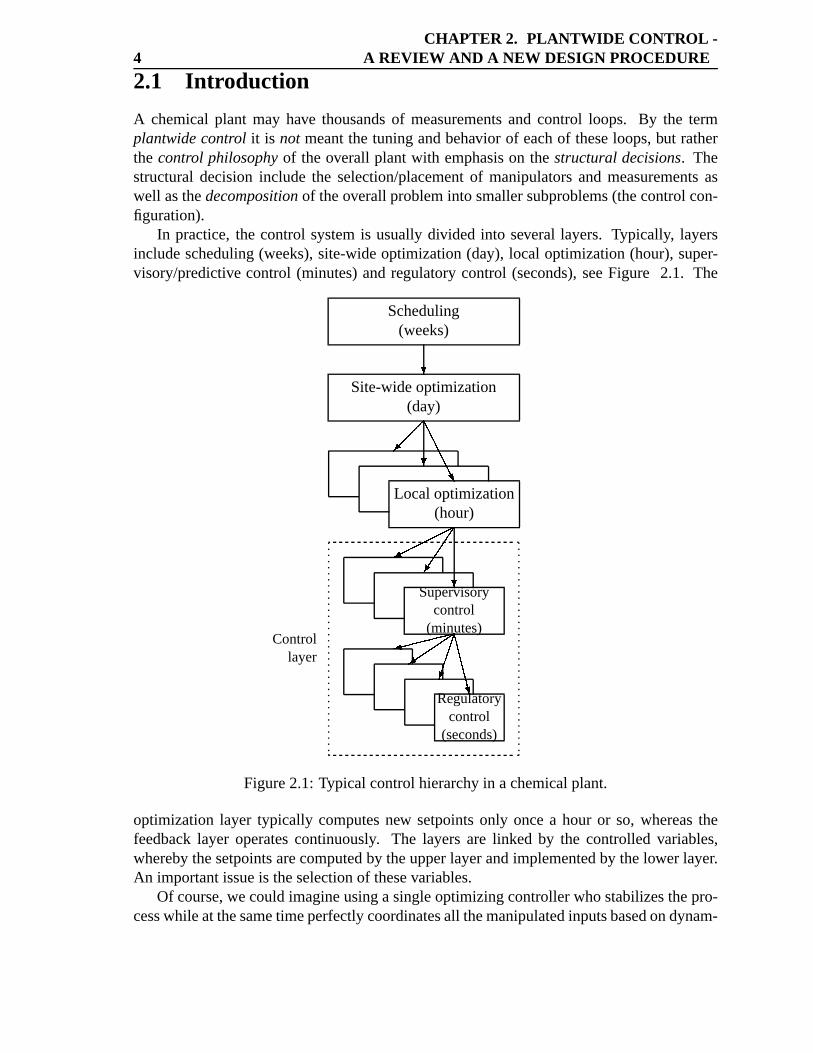
In practice,the control systemis usuallydivided into several layers. Typically, layersincludescheduling(weeks),site-wideoptimization(day), local optimization(hour),super-visory/predictive control (minutes)andregulatorycontrol (seconds),seeFigure 2.1. The
�Scheduling
(weeks)
Site-wideoptimization(day)� � � � �
Localoptimization(hour)
���� �
�Supervisory
control(minutes)
���� � ����� �� � � � ��
Regulatorycontrol
(seconds)
���� � ���� � ����� �Controllayer
Figure2.1: Typical controlhierarchyin achemicalplant.
optimizationlayer typically computesnew setpointsonly oncea hour or so, whereasthefeedbacklayer operatescontinuously. The layersare linked by the controlledvariables,wherebythesetpointsarecomputedby theupperlayerandimplementedby thelower layer.An importantissueis theselectionof thesevariables.
Of course,wecouldimagineusingasingleoptimizingcontrollerwhostabilizesthepro-cesswhile atthesametimeperfectlycoordinatesall themanipulatedinputsbasedondynam-
2.1. INTRODUCTION 5
ic on-lineoptimization.Therearefundamentalreasonswhy sucha solutionis not thebest,evenwith today’s andtomorrows computingpower. Onefundamentalreasonis thecostofmodeling,andthefactthatfeedbackcontrol,withoutmuchneedfor models,is veryeffectivewhenperformedlocally. In fact,by cascadingfeedbackloops,it is possibleto control largeplantswith thousandsof variableswithout theactualneedto developany models.However,thetraditionalsingle-loopcontrolsystemscansometimesberathercomplicated,especiallyif thecascadesareheavily nestedor if thepresenceof constraintsduringoperationmake itnecessaryto uselogic switches.Thus,modelbasedcontrol shouldbeusedwhenthemod-elingeffort givesenoughpay-backin termsof simplicity and/orimprovedperformance,andthis will usuallybeat thehigherlayersin thecontrolhierarchy.
A very important(if not themostimportant)problemin plantwidecontrolis theissueofdeterminingthecontrol structure: Which “boxes”shouldwehaveandwhatinformationshouldbesendbetweenthem?
Note that that we areherenot interestedin what shouldbe insidethe boxes,which is thecontrollerdesignor tuning problem. More precisely, control structure design is definedasthestructural decisionsinvolved in controlsystemdesign,including thefollowing tasks((Foss,1973);(Morari, 1982);(SkogestadandPostlethwaite,1996))
1. Selectionof controlledoutputs� (variableswith setpoints)
2. Selectionof manipulatedinputs �3. Selectionof measurements� (for controlpurposesincludingstabilization)
4. Selectionof control configuration (astructureinterconnectingmeasurements/setpointsandmanipulatedvariables,i.e. thestructureof thecontroller � which interconnectsthevariables��� and � (controllerinputs)with thevariables� )
5. Selectionof controller type(controllaw specification,e.g.,PID,decoupler, LQG,etc.).
In mostcasesthecontrolstructuredesignis solvedby amixtureof a top-down considerationof controlobjectivesandwhich degreesof freedomareavailableto meetthese(tasks1 and2), andawith abottom-updesignof thecontrolsystem,startingwith thestabilizationof theprocess(tasks3,4and5).
In mostcasesthe problemis solved without the useof any theoreticaltools. In fact,the industrialapproachto plantwidecontrol is still very muchalongthe linesdescribedbyPageBuckley in his bookfrom 1964.Of course,thecontrolfield hasmademany advancesover theseyears,for example,in methodsfor andapplicationsof on-lineoptimizationandpredictive control. Advanceshave alsobeenmadein control theoryandin the formulationof tools for analyzingthe controllability of a plant. Theselatter tools canbe mosthelpfulin screeningalternative control structures. However, a systematicmethodfor generatingpromisingalternative structureshasbeenlacking. This is relatedto the fact thatplantwidecontrolproblemitself hasnotbeenwell understoodor evenacknowledgedasimportant.
Thecontrolstructuredesignproblemis difficult to definemathematically, bothbecauseof thesizeof theproblem,andthelargecostinvolvedin makingapreciseproblemdefinition,
6CHAPTER 2. PLANTWIDE CONTROL -
A REVIEW AND A NEW DESIGN PROCEDURE
whichwouldinclude,for example,adetaileddynamicandsteadystatemodel.An alternativeto this is to developheuristicrulesbasedon experienceandprocessunderstanding.This iswhatwill bereferredto astheprocessoriented approach.
Therealizationthatthefield of controlstructuredesignis underdevelopedis not new. Inthe1970’s several “critique” articleswherewritten on thegapbetweentheoryandpracticein the areaof processcontrol. The mostfamousis the oneof (Foss,1973)who madetheobservationthatin many areasapplicationwasaheadof theory, andhestatedthat
The centralissuesto be resolved by the new theoriesarethe determinationofthecontrolsystemstructure.Whichvariablesshouldbemeasured,which inputsshouldbemanipulatedandwhich links shouldbe madebetweenthe two sets?... The gap is presentindeed,but contraryto the views of many, it is thetheoreticianwho mustcloseit.
A similar observation that applicationsseemto be aheadof formal theory was madebyFindeisenetal. (1980)in theirbookon hierarchicalsystems(p. 10).
Many authorspoint out that the needfor a plantwideperspective on control is mainlydueto changesin theway plantsaredesigned– with moreheatintegrationandrecycle andlessinventory. Indeed,thesefactorsleadto moreinteractionsandthereforethe needfor aperspective beyondindividual units. However, we would like to point out thatevenwithoutany integrationthereis still a needfor a plantwideperspective asa chemicalplantconsistsof a stringof unitsconnectedin series,andoneunit will actasadisturbanceto thenext, forexample,all unitsmusthave thesamethroughputat steady-state.
Outline
We will first discussin moredetail someof the termsusedabove andprovide somedefini-tions.We thenpresenta review of someof thework onplantwidecontrol. In section2.4wediscussthemathematicallyorientedapproach(controlstructuredesign).Then,in section2.5we look at the processorientedapproach.In section2.6 we considera fairly simpleplan-t consistingof reactor, separatorandrecycle. In section2.7 we considerthe moststudiedplantwidecontrol problem,namelythe TennesseeEastmanproblemintroducedby DownsandVogel(1993),andwediscusshow variousauthorshaveattemptedto solve theproblem.Finally, in section2.8weproposeanew plantwidecontroldesignprocedure.
2.2 Termsand definitions
We heremake somecommentson the termsintroducedabove, andalsoattemptto providesomemoreprecisedefinitions,of thesetermsandsomeadditionalones.
Let us first considerthe termsplant andprocess, which arealmostsynonymousterms.In thecontrolcommunityasawhole,thetermplantis somewhatmoregeneralthanprocess:A processusuallyrefersto the“processitself” (withoutany controlsystem)whereasaplantmaybeanysystemto becontrolled (includingapartiallycontrolledprocess).However, note
2.2. TERMS AND DEFINITIONS 7
that in thechemicalengineeringcommunitythetermplanthasa somewhatdifferentmean-ing, namelyasthewholefactory, which consistsof many processunits; thetermplantwidecontrolis derivedfrom this meaningof theword plant.
Let us thendiscussthe two closelyrelatedtermslayer and level which areusedin hi-erarchicalcontrol. Following the literaturee.g. Findeisenet al. (1980)the correctterm inour context is layer. In a layerthepartsactsat differenttimescalesandeachlayerhassomefeedbackor informationfrom theprocessandfollows setpointsgivenfrom layersabove. Alower layer may not know the criterion of optimality by which the setpointhasbeenset.A multi-layersystemcannotbestrictly optimalbecausetheactionsof thehigherlayersarediscreteandthusunableto follow strictly theoptimalcontinuoustimepattern.(Ontheotherhand,in a multilevel systemthereis no time scaleseparationandthe partsarecoordinat-ed suchthat thereareno performanceloss. Multilevel decompositionmay be usedin theoptimizationalgorithmbut otherwiseis of no interesthere.)
Control is the adjustmentof available degreesof freedom(manipulatedvariables)toassistin achieving acceptableoperationof theplant. Controlsystemdesignmaybedividedinto threemainactivities
1. Controlstructuredesign(structuraldecisions)
2. Controllerdesign(parametricdecisions)
3. Implementation
Thetermcontrol structure design, which is commonlyusedin thecontrolcommunity,refersto thestructuraldecisionsin thedesignof thecontrolsystem.It is definedby thefivetasks(givenin theintroduction):
1. Selectionof controlledoutputs( � with setpoints��� ).2. Selectionof manipulatedinputs( � ).
3. Selectionof measurements( � )4. Selectionof control configuration
5. Selectionof controller type
Theresultfrom thecontrol structuredesignis thecontrol structure(alternativelydenotedthecontrol strategyor control philosophyof theplant).
The term plantwidecontrol is usedonly in the processcontrol community. Onecouldregardplantwidecontrol asthe“processcontrol” versionof controlstructuredesign,but thisis probablyabit too limiting. In fact,RinardandDowns(1992)referto thecontrolstructuredesignproblemasdefinedaboveasthe“strict definitionof plantwidecontrol”, andthey pointout that plantwidecontrol also include important issuessuchas the operatorinteraction,startup,grade-change,shut-down, fault detection,performancemonitoring and designofsafetyandinterlock systems.This is morein line with the discussionby Stephanopoulos,(1982).
8CHAPTER 2. PLANTWIDE CONTROL -
A REVIEW AND A NEW DESIGN PROCEDURE
Maybe a betterdistinction is the following: Plantwidecontrol refersto the structuralandstrategic decisionsinvolved in the control systemdesignof a completechemicalplant(factory),andcontrol structuredesignis thesystematic(mathematical)approachfor solvingthis problem.
Thecontrol configuration, is definedastherestrictionsimposedby theoverallcontroller� by decomposingit into asetof localcontrollers(sub-controllers),units,elements,blocks)with predeterminedlinks and possiblywith a predetermineddesignsequencewheresub-controllersaredesignedlocally.
Operation involvesthebehavior of thesystemonceit hasbeenbuild, andthis includesalot morethancontrol. More precisely, thecontrolsystemis designedto aid theoperationoftheplant. Operability is theability of theplant(togetherwith its controlsystem)to achieveacceptableoperation(both staticallyanddynamically). Operability includesswitchabilityandcontrollabilityaswell asmany otherissues.
Flexibility refersto theability to obtainfeasiblesteady-stateoperationat a givensetofoperatingpoints. This is a steady-stateissue,andwe will assumeit to be satisfiedat theoperatingpointsweconsider. It is not consideredany furtherin this paper.
Switchability refersto theability to go from oneoperatingpoint to anotherin anaccept-ablemannerusuallywith emphasison feasibility. It is relatedto othertermssuchasoptimaloperationandcontrollability for largechanges,andis notconsideredexplicitly in thispaper.
Wewill assumethatthe“quality (goodness)of operation”canbequantifiedin termsof ascalarperformanceindex (objective function) , which shouldbeminimized.For example, canbetheoperatingcosts.
Optimaloperation usuallyrefersto thenominallyoptimalway of operatinga plantasitwould resultby applyingsteady-stateand/ordynamicoptimizationto a modelof theplant(with nouncertainty),attemptingto minimizethecost by adjustingthedegreesof freedom.
In practice,we cannotobtainoptimal operationdueto uncertainty. The differencebe-tweenthe actualvalueof the objective function and its nominally optimal value is theloss.
Thetwo mainsourcesof uncertaintyare(1) signaluncertainty(includesdisturbances( ! )andmeasurementnoise( " )) and(2) modeluncertainty.
Robustmeansinsensitive to uncertainty. Robustoptimaloperation is theoptimalway ofoperatinga plant(with uncertaintyconsiderationsincluded).
Integratedoptimizationandcontrol (or optimizingcontrol)refersto a systemwhereop-timizationandits control implementationareintegrated.In theory, it shouldbepossibletoobtainrobustoptimaloperationwith sucha system.In practice,oneoftenusesa hierarchi-cal decompositionwith separatelayersfor optimizationandcontrol. In makingthis split weassumethatfor thecontrolsystemthegoalof “acceptableoperation”hasbeentranslatedinto“keepingthecontrolledvariables( � ) within specifiedboundsfrom their setpoints( ��� )”. Theoptimizationlayersendssetpointvalues( ��� ) for selectedcontrolledoutputs( � ) to thecontrollayer. Thesetpointsareupdatedonly periodically. (Thetasks,or partsof thetasks,in eitherof theselayersmay be performedby humans.)The control layer may be further divided,e.g. into supervisorycontrolandregulatorycontrol. In general,in a hierarchicalsystem,thelower layerswork ona shortertimescale.
In additionto keepingthecontrolledvariablesat their setpoints,thecontrolsystemmust
2.2. TERMS AND DEFINITIONS 9
“stabilize” the plant. We have hereput stabilizein quotesbecausewe usethe word in anextendedmeaning,and includeboth modeswhich aremathematicallyunstableaswell asslow modes(“drift”) that needto be “stabilized” from an operatorpoint of view. Usual-ly, stabilizationis donewithin a separate(lower) layer of the control system,often calledthe regulatorycontrol layer. The controlledoutputsfor stabilizationaremeasuredoutputvariables,andtheir setpointsmaybeusedasdegreesof freedomfor thelayersabove.
For eachlayer in a control systemwe usethe termscontrolled output ( # with setpoint# � ) andmanipulatedinput ( $ ). Correspondingly, the term “plant” refersto the systemtobe controlled(with manipulatedinputs $ andcontrolledoutputs # ). The layersareoftenstructuredhierarchically, suchthatthemanipulatedinputfor ahigherlayer( $ � ) is thesetpointfor a lower layer ( # � � ), i.e. # � �&% $ � . (Thesecontrolledoutputsneedin generalnot bemeasuredvariables,andthey mayincludesomeof themanipulatedinputs( $ ).)
Fromthisweseethattheterms“plant”, “controlledoutput” ( # ) and“manipulatedinput”( $ ) takeson differentmeaningdependingon wherewe arein thehierarchy. To avoid con-fusion,we reserve specialsymbolsfor thevariablesat the top andbottomof thehierarchy.Thus,asalreadymentioned,thetermprocessis oftenusedto denotetheuncontrolledplantasseenfrom thebottomof thehierarchy. Herethemanipulatedinputsarethephysicalmanipu-lators(e.g.valvepositions),andaredenoted� . Correspondingly, at thetopof thehierarchy,we usethesymbol � to denotethecontrolledvariablesfor which thesetpointvalues( ��� ) aredeterminedby theoptimizationlayer.
Input-Outputcontrollability of aplantis theability to achieveacceptablecontrolperfor-mance,thatis, to keepthecontrolledoutputs( # ) within specifiedboundsfrom theirsetpoints( ' ), in spiteof signaluncertainty(disturbances! , noise" ) andmodeluncertainty, usingavail-ableinputs( $ ) andavailablemeasurements.In otherwords,theplantis controllableif thereis acontrollerthatsatisfiesthecontrolobjectives.
This definitionof controllability maybeappliedto thecontrolsystemasa whole,or topartsof it (in the casethe control layer is structured). The term controllability generallyassumesthat we usethebestpossiblemultivariablecontroller, but we may imposerestric-tionson theclassof allowedcontrollers(e.g.consider“controllability with decentralizedPIcontrol”).
A plantis self-regulatingif wewith constantinputscankeepthecontrolledoutputswithinacceptablebounds. (Note that this definition may be appliedto any layer in the controlsystem,sotheplantmaybeapartially controlledprocess).“True” self-regulationis definedasthecasewhereno control is ever neededat thelowestlayer(i.e. � is constant).It relieson theprocessto dampenthedisturbancesitself, e.g.by having largebuffer tanks.Werarelyhave “true” self-regulationbecauseit maybeverycostly.
Self-optimizingcontrol is whenan acceptablelosscanbe achieved usingconstantset-pointsfor thecontrolledvariables(without theneedto reoptimizewhendisturbancesoccur).“True” self-optimizationis definedasthecasewhereno re-optimizationis ever needed(so��� canbekeptconstantalways),but thisobjective is usuallynotsatisfied.Ontheotherhand,we must requirethat the processis self-optimizingwithin the time period betweeneachre-optimization,or elsewecannotuseseparatecontrolandoptimizationlayers.
A processis self-optimizingif thereexists a set of controlledoutputs( � ) suchthat ifwe with keepconstantsetpointsfor theoptimizedvariables( ��� ), thenwe cankeepthe loss
10CHAPTER 2. PLANTWIDE CONTROL -
A REVIEW AND A NEW DESIGN PROCEDURE
within anacceptableboundwithin aspecifiedtimeperiod.A steady-stateanalysisis usuallysufficient to analyzeif we have self-optimality. This is basedon the assumptionthat theclosed-looptimeconstantof thecontrolsystemis smallerthanthetimeperiodbetweeneachre-optimization(so that it settlesto a new steady-state)andthat the valueof the objectivefunction ( ) is mostly determinedby the steady-statebehavior (i.e. there is no “costly”dynamicbehavior e.g.imposedby poorcontrol).
Mostof thetermsgivenabovearein standarduseandthedefinitionsmostlyfollow thoseof SkogestadandPostlethwaite(1996).
2.3 General reviewsand bookson plantwide control
We herepresenta brief review of someof the previous reviews and bookson plantwidecontrol.
Morari (1982)presentsa well-written review on plantwidecontrol,wherehe discusseswhy moderncontrol techniqueswere not (at that time) in widespreadusein the processindustry. Thefour mainreasonswerebelievedto be
1. Largescalesystemaspects.
2. Sensitivity (robustness).
3. Fundamentallimitationsto controlquality.
4. Education.
He thenproceedsto look athow two waysof decomposetheproblem:
1. Multi-layer (vertical),wherethedifferencebetweenthelayersarein thefrequency ofadjustmentof theinput.
2. Horizontaldecomposition,wherethesystemis dividedinto noninteractingparts.
Stephanopoulos(1982)statesthatthesynthesisof a controlsystemfor a chemicalplantis still to a large extent an art. He asks: “Which variablesshouldbe measuredin orderto monitor completelythe operationof a plant? Which input shouldbe manipulatedforeffective control? How shouldmeasurementsbepairedwith themanipulationsto form thecontrol structure,and finally, what the control laws are?” He notesthat the problemofplantwidecontrol is “multi-objective” and“there is a needfor a systematicandorganizedapproachwhichwill identify all necessarycontrolobjectives”. Thearticleis comprehensive,anddiscussesmany of theproblemsin thesynthesisof controlsystemsfor chemicalplants.
RinardandDowns (1992) review muchof the relevant work in the areaof plantwidecontrol,andthey alsoreferto importantpapersthatwehavenot referred.They concludethereview by statingthat “the problemprobablynever will besolvedin thesensethata setofalgorithmswill leadto thecompletedesignof a plantwidecontrol system”. They suggeststhatmorework shouldbedoneon thefollowing items: (1) A way of answeringwhetherornot thecontrolsystemwill meetall theobjectives,(2) Sensorselectionandlocation(where
2.4. CONTROL STRUCTURE DESIGN (THE MATHEMA TICALL Y ORIENTEDAPPROACH) 11
they indicatethattheoryon partialcontrolmaybeuseful),(3) Processeswith recycle. Theyalsowelcomecomputer-aidedtools,bettereducationandgoodnew testproblems.
The book by Balchenand Mumme (1988) attemptsto combineprocessand controlknowledge,andto usethis to designcontrolsystemsfor somecommonunit operationsandalsoconsiderplantwidecontrol. The book providesmany practicalexamples,but thereislittle in termsof analysistoolsor asystematicframework for plantwidecontrol.
The book “Integratedprocesscontrol and automation”by Rijnsdorp(1991), containsseveral subjectsthatarerelevanthere. Part II in thebook is on optimaloperation.He dis-tinguishesbetweentwo situations,sellersmarked(maximizeproduction)andbuyersmarked(producea givenamountat lowestpossiblecost). He alsohasa procedurefor designof anoptimizingcontrolsystem.
Loe(1994)presentsasystematicwayof lookingatplantswith thefocusis on functions.Theauthorcovers“qualitative” dynamicsandcontrolof importantunit operations.
van de Wal andde Jager(1995) list several criteria for evaluationof control structuredesignmethods:generality, applicableto nonlinearcontrolsystems,controller-independent,direct, quantitative, efficient, effective, simpleandtheoreticallywell developed. After re-viewing they concludethatsuchamethoddoesnot exist.
The book by Skogestadand Postlethwaite (1996) hastwo chapterson controllabilityanalysisandonechapteroncontrolstructuredesign.Particularlyin chapter10 thereis sometopics,which arerelevant for plantwidecontrol, amongthemarepartial control andself-optimizingcontrol(a termintroducedlater).
The coming monographby Ng and Stephanopoulos(1998a) dealsalmostexclusivelywith plantwidecontrol.
The book by Luybenet al. (1998)hascollectedmuchof Luyben’s practicalideasandsummarizedthemin aclearmanner. Theemphasisis on casestudies.
Therealsoexistsa largebodyof system-theoreticliteraturewithin thefield of large-scalesystems,but mostof it haslittle relevanceto plantwidecontrol. Oneimportantexceptionisthe bookby Findeisenet al. (1980)on “Control andcoordinationin hierarchicalsystems”which probablydeservesto bestudiedmorecarefullyby theprocesscontrolcommunity.
2.4 Control Structur e Design(The mathematically orient-edapproach)
In this sectionwe look at themathematicallyorientedapproachto plantwidecontrol.
Structural methods
Therearesomemethodsthatusestructuralinformationabouttheplantasabasisfor controlstructuredesign.For a recentreview of thesemethodswe refer to the comingmonographof Ng andStephanopoulos(1998a). Centralconceptsarestructuralstatecontrollability, ob-servability andaccessibility. Basedonthis,setsof inputsandmeasurementsareclassifiedasviableor non-viable.Althoughthestructuralmethodsareinteresting,they arenot quantita-
12CHAPTER 2. PLANTWIDE CONTROL -
A REVIEW AND A NEW DESIGN PROCEDURE
tiveandusuallyprovide little informationotherthanconfirminginsightsaboutthestructureof theprocessthatmostengineersalreadyhave.
In the reminderof this sectionwe discussthe five tasksof the control structuredesignproblem,listedin theintroduction.
2.4.1 Selectionof controlled outputs ( ( )By “controlledoutputs”weherereferto thecontrolledvariables� for which thesetpoints���aredeterminedby theoptimizationlayer. Therewill alsobeother(internally)controlledout-putswhich resultfrom thedecompositionof thecontrollerinto blocksor layers(includingcontrolledmeasurementsusedfor stabilization),but thesearerelatedto thecontrolconfigu-rationselection,which is discussedaspartof task4.
Theissueof selectionof controlledoutputs,is probablythe leaststudiedof thetasksinthecontrolstructuredesignproblem.In fact,it seemsfrom our experiencethatmostpeopledonotconsiderit asbeinganissueatall. Themostimportantreasonfor this is probablythatit is a structuraldecisionfor which therehasnot beenmuchtheory. Thereforethedecisionhasmostlybeenbasedonengineeringinsightandexperience,andthevalidity of theselectionof controlledoutputshasseldombeenquestionedby thecontroltheoretician.
To seethattheselectionof outputis anissue,askthequestion:
Whyare wecontrolling hundredsof temperatures,pressuresandcompositionsin a chemicalplant,whenthere is no specificationon mostof thesevariables?
After somethought,onerealizesthat the main reasonfor controlling all thesevariablesisthatoneneedsto specifytheavailabledegreesof freedomin orderto keeptheplantclosetoits optimaloperatingpoint. But thereis a follow-upquestion:
Whydo weselecta particular set � of controlled variables? (e.g., whyspecify(control) the top compositionin a distillation column,which doesnot producefinal products,ratherthanjust specifyingits reflux?)
Theanswerto this secondquestionis lessobvious,becauseat first it seemslike it doesnotreally matterwhich variableswe specify(aslong asall degreesof freedomareconsumed,becausethe remainingvariablesarethenuniquelydetermined).However, this is true onlywhenthereis nouncertaintycausedby disturbancesandnoise(signaluncertainty)or modeluncertainty. Whenthereis uncertaintythen it doesmake a differencehow the solution isimplemented,thatis, whichvariablesweselectto controlat their setpoints.
Self-optimizing control
Thebasicideaof whatwe have calledself-optimizingcontrolwasformulatedabouttwentyyearsagoby Morari et al. (1980):
“in attemptingto synthesizea feedbackoptimizing control structure,our mainobjective is to translatetheeconomicobjectivesinto processcontrolobjectives.In otherwords,wewantto finda function � of theprocessvariableswhich when
2.4. CONTROL STRUCTURE DESIGN (THE MATHEMA TICALL Y ORIENTEDAPPROACH) 13
heldconstant,leadsautomaticallyto theoptimaladjustmentsof themanipulatedvariables,andwith it, theoptimaloperatingconditions. [...] Thismeansthatbykeepingthefunction �*) $,+-!/. atthesetpoint��� , throughtheuseof themanipulatedvariables$ , for variousdisturbances! , it follows uniquely that the processisoperatingat theoptimalsteady-state.”
If we replacethe term “optimal adjustments”by “acceptableadjustments(in termsof theloss)”thentheaboveisaprecisedescriptionof whatSkogestad(2000)denoteaself-optimizingcontrolstructure.Theonly factorMorari et al. (1980)fail to consideris theeffectof theim-plementationerror �102��� . Morari et al. (1980)proposeto selectthe bestsetof controlledvariablesbasedon minimizing theloss(“feedbackoptimizingcontrolcriterion1”).
Somewhat surprisingly, the ideasof Morari et al. (1980) received very little attention.Onereasonis probablythat thepaperalsodealtwith the issueof finding theoptimaloper-ation (andnot only on how to implementit), andanotherreasonis that the only examplein the paperhappenedto result in an implementationwith the controlledvariablesat theirconstraints.Theconstrainedcaseis “easy” from an implementationpoint of view, becausethesimplestandoptimal implementationis to simply maintaintheconstrainedvariablesattheir constraints.No examplewasgivenfor themoredifficult unconstrainedcase,wherethechoiceof controlled(feedback)variablesis a critical issue.The follow-up paperby ArkunandStephanopoulos(1980)concentratedfurtheron theconstrainedcaseandtrackingof ac-tiveconstraints.
SkogestadandPostlethwaite(1996)(Chapter10.3)presentanapproachfor selectingcon-trolled outputsimilar to thoseof Morari et al. (1980)andtheideaswherefurtherdevelopedin (Skogestad,2000)wherethetermself-optimizingcontrolis introduced.Skogestad(2000)stressestheneedto considerthe implementationerrorwhenevaluatingthe loss. Skogestad(2000)givesfour requirementsthata controlledvariableshouldmeet: 1) Its optimalvalueshouldbeinsensitiveto disturbances.2) It shouldbeeasyto measureandcontrolaccurately.3) Its valueshouldbe sensitive to changesin themanipulatedvariables.4) For caseswithtwo or morecontrolledvariables,theselectedvariablesshouldnotbecloselycorrelated.Byscalingof the variablesproperly, SkogestadandPostlethwaite (1996)shows that the self-optimizingcontrolstructureis relatedto maximizingtheminimumsingularvalueof thegainmatrix , where3 �4% 35$ . Zhengetal. (1999)alsousetheideasof Morari etal. (1980)asabasisfor selectingcontrolledvariables.Therelationshipto thework of Shinnaris discussedseparatelylater.
Other work
In his book Rijnsdorp(1991)giveson page99 a stepwisedesignprocedurefor designingoptimizing control systemsfor processunits. One stepis to “transfer the result into on-line algorithmsfor adjustingthe degreesof freedomfor optimization”. He statesthat this“requiresgoodprocessinsightandcontrolstructureknow-how. It is worthwhilebasingthealgorithmasfar aspossibleon processmeasurements.In any case,it is impossibleto giveaclear-cut recipehere.”
Fisheret al. (1988a) discussplanteconomicsin relationto control. They provide someinterestingheuristicideas.In particular, hiddenin theirHDA examplein part3 (p. 614)one
14CHAPTER 2. PLANTWIDE CONTROL -
A REVIEW AND A NEW DESIGN PROCEDURE
findsaninterestingdiscussionontheselectionof controlledvariables,which is quitecloselyrelatedto theideasof Morari et al. (1980).
Luyben(1988)introducedtheterm“eigenstructure”to describetheinherentlybestcon-trol structure(with thebestself-regulatingandself-optimizingproperty). However, hedidnot really definetheterm,andalsothenameis unfortunatesince“eigenstructure”hasa an-otherunrelatedmathematicalmeaningin termsof eigenvalues.Apart from this,Luybenandcoworkers(e.g. Luyben(1975),Yi andLuyben(1995))have studiedunconstrainedprob-lems,andsomeof the examplespresentedpoint in the directionof the selectionmethodspresentedin this paper. However, Luybenproposesto selectcontrolledoutputswhich mini-mizesthesteady-statesensitiveof themanipulatedvariable( $ ) to disturbances,i.e. to selectcontrolledoutputs( � ) suchthat )76 $98 6 !/.;: is small,whereaswe really want to minimize thesteady-statesensitivity of the economicloss ( < ) to disturbances,i.e. to selectcontrolledoutputs( � ) suchthat )76 <=8 6 !/.;: is small.
Narrawayetal. (1991),NarrawayandPerkins(1993)andNarrawayandPerkins(1994))stronglystresstheneedto basetheselectionof thecontrolstructureon economics,andtheydiscussthe effect of disturbanceson the economics.However, they do not formulateanyrulesor proceduresfor selectingcontrolledvariables.
Finally Mizoguchi et al. (1995)andMarlin andHrymak (1997)stressthe needto finda goodway of implementingthe optimal solutionin termshow the control systemshouldrespondto disturbances,“i.e. thekey constraintsto remainactive,variablesto bemaximizedor minimized,priority for adjustingmanipulatedvariables,andsoforth.” They suggestthatan issuefor improvementin today’s real-timeoptimizationsystemsis to selectthecontrolsystemthat yields the highestprofit for a rangeof disturbancesthat occur betweeneachexecutionof theoptimization.
Therehasalsobeendonesomework on non-squareplants,i.e. with moreoutputsthaninputs,e.g. (Cao,1995)and(ChangandYu, 1990). Theseworksassumesthat thecontrolgoal is the keepall thesevariablesascloseto “zero” aspossible,andoften the effect ofdisturbancesis not considered.It maybemoresuitableto reformulatetheseproblemsintotheframework of self-optimizingcontrol.
2.4.2 Selectionof manipulated inputs ( > )
By manipulatedinputswe referto thephysicaldegreesof freedom,typically thevalveposi-tionsor electricpower inputs. Actually, selectionof thesevariablesis usuallynot muchofanissueat thestageof controlstructuredesign,sincethesevariablesusuallyfollow asdirectconsequenceof thedesignof theprocessitself.
However, theremaybesomepossibilityof addingvalvesor moving them.For example,if we install a bypasspipelineanda valve, thenwe may usethe bypassflow asan extradegreeof freedomfor controlpurposes.
Finally, let us make it clearthat the possibility of not actively usingsomemanipulatedinputs(or only changingthemrarely), is a decisionthat is includedabove in “selectionofcontrolledoutputs”.
2.4. CONTROL STRUCTURE DESIGN (THE MATHEMA TICALL Y ORIENTEDAPPROACH) 15
2.4.3 Selectionof measurements( ? )
Controllability considerations,including dynamicbehavior, are importantwhen selectingwhich variablesto measure.Thereare often many possiblemeasurementswe canmake,and the number, locationand accuracy of the measurementis a tradeoff betweencost ofmeasurementsand benefitsof improved control. A controllability analysismay be veryuseful. In most casesthe selectionof measurementsmust be consideredsimultaneouslywith the selectionof the control configuration. For example,this appliesto the issueofstabilizationandtheuseof secondarymeasurements.
2.4.4 Selectionof control configuration
Theissueof controlconfigurationselection,includingdecentralizedcontrol,is discussedinHovd andSkogestad(1993)andin sections10.6,10.7and10.8of SkogestadandPostleth-waite(1996),andwewill herediscussmainly issueswhicharenotcoveredthere.
Thecontrolconfigurationis thestructureof thecontroller � thatinterconnectsthemea-surements,setpoints��� andmanipulatedvariables� . Thecontrollercanbestructured(de-composed)into blocksboth in anvertical (hierarchical)andhorizontal(decentralizedcon-trol) manner.
Why is thecontrollerdecomposed?(1) Thefirst reasonis thatit mayrequirelesscompu-tation.This reasonmayberelevantin somedecision-makingsystemswherethereis limitedcapacityfor transmittingandhandlinginformation(like in mostsystemswherehumansareinvolved),but it doesnothold in today’schemicalplantwhereinformationis centralizedandcomputingpower is abundant. Two otherreasonsoften givenare(2) failure toleranceand(3) theability of localunitsto actquickly to rejectdisturbances(e.g.Findeisenetal., 1980).Thesereasonsmaybemorerelevant,but,aspointedoutby SkogestadandHovd (1995)thereareprobablyotherevenmorefundamentalreasons.Themostimportantoneis probably(4)to reducethe cost involved in definingthe control problemandsettingup the detaileddy-namicmodelwhich is requiredin a centralizedsystemwith no predeterminedlinks. Also,(5) decomposedcontrol systemsare much lesssensitive to modeluncertainty(sincetheyoftenusenoexplicit model).In otherwords,by imposingacertaincontrolconfiguration,weareimplicitly providing processinformation,which we with a centralizedcontrollerwouldneedto supplyexplicitly throughthemodel.
Stabilizing control
Instability requirestheactive useof manipulatedinputs( � ) usingfeedbackcontrol. Thereexist relatively few systematictools to assistin selectinga control structurefor stabilizingcontrol. Usually, single-loopcontrollersare usedfor stabilization,and issuesare whichvariablesto measureand which manipulatedinputs to use. One problemin stabilizationis that measurementnoisemay causelarge variationsin the input such that it saturates.Havre andSkogestad(1996,1998)have shown that thepolevectors maybeusedto selectmeasurementsandmanipulatedinputssuchthatthis problemis minimized.
16CHAPTER 2. PLANTWIDE CONTROL -
A REVIEW AND A NEW DESIGN PROCEDURE
Secondarymeasurements
Extra(secondary)measurementsareoftenaddedto improve thecontrol. Threealternativesfor useof extrameasurementsare:
1. Centralizedcontroller: All themeasurementsareusedto computetheoptimal input.Thiscontrollerhasimplicitly anestimator(model)hiddeninsideit.
2. Inferentialcontrol:Basedonthemeasurementsamodelis usedto provideanestimateof theprimaryoutput(e.g. a controlledoutput � ). This estimateis sendto a separatecontroller.
3. Cascadecontrol: The secondarymeasurementsare controlledlocally and their set-pointsareusedasdegreesof freedomat somehigherlayerin thehierarchy.
Notethatbothcentralizedandinferentialcontrolusestheextrameasurementsto estimateparametersin amodel,whereascascadedcontrolthey areusedfor additionalfeedback.Thesubjectof estimationandmeasurementsselectionfor estimationis beyondthescopeof thisreview article; we refer to Ljung (1987) for a control view and to Martens(1989) for achemometricsapproachto this issue. However, we would like point out that the controlsystemshouldbe designedfor bestpossiblecontrol of the primary variables( � ), andnotthebestpossibleestimate.A drawbackof the inferentialschemeis thatestimateis usedinfeed-forwardmanner.
For cascadecontrolHavre(1998)hasshown how to selectsecondarymeasurementssuchthattheneedfor updatingthesetpointsis small.Theissuesherearesimilar to thatof select-ing controlledvariables( � ) discussedabove. Oneapproachis to minimizesomenormof thetransferfunctionfrom thedisturbanceandcontrolerrorin thesecondaryvariableto thecon-trol errorin theprimaryvariable.A simpler, but lessaccurate,alternative is to maximizetheminimumsingularvaluein thetransferfunctionfrom secondarymeasurementsto the inputusedto controlthesecondarymeasurements.LeeandMorari ((LeeandMorari, 1991),(Leeetal., 1995)and(Leeetal., 1997))consideredasimilarproblem.They usedamorerigorousapproachwheremodeluncertaintyis explicitly consideredandthestructuredsingularvalueis usedasa tool.
Partial control
Most control configurationsare structuredin a hierarchicalmannerwith fast inner loops,andslower outerloopsthatadjustthesetpointsfor the inner loops. Control systemdesigngenerallystartsby designingthe inner (fast) loops, and then outer loops are closedin asequentialmanner. Thus, the designof an “outer loop” is doneon a partially controlledsystem.Wehereprovidesomesimplebut yetveryusefulrelationshipsfor partiallycontrolledsystems.Wedivide theoutputsinto two classes: # � – (temporarily)uncontrolledoutput # � – (locally) measuredandcontrolledoutput(in theinnerloop)
2.4. CONTROL STRUCTURE DESIGN (THE MATHEMA TICALL Y ORIENTEDAPPROACH) 17
We have insertedthe word temporarily above, since # � is normally a controlledoutputatsomehigherlayer in thehierarchy. We alsosubdivide theavailablemanipulatedinputsin asimilar manner: $ � – inputsusedfor controlling # � (in theinnerloop) $ � – remaininginputs(which maybeusedfor controlling # � )
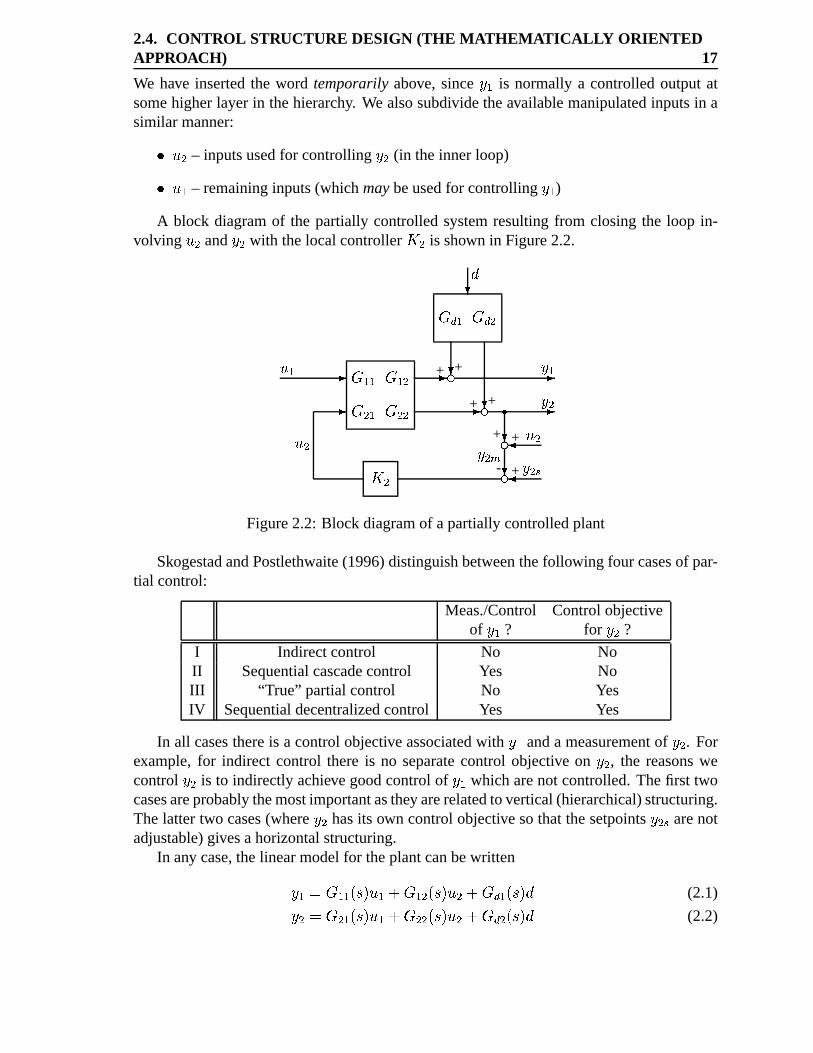
A block diagramof the partially controlledsystemresultingfrom closing the loop in-volving $ � and # � with thelocal controller � � is shown in Figure2.2.
@@$ � ��� ��� �A� ���
� !CB � CB �� �
� �$ �@ @D+ + D+ + D+ +D- +
@# �@# �E��# �GF " �HH # � �Figure2.2: Block diagramof apartially controlledplant
SkogestadandPostlethwaite(1996)distinguishbetweenthefollowing four casesof par-tial control:
Meas./Control Controlobjectiveof # � ? for # � ?
I Indirectcontrol No NoII Sequentialcascadecontrol Yes NoIII “True” partialcontrol No YesIV Sequentialdecentralizedcontrol Yes Yes
In all casesthereis a controlobjective associatedwith # � anda measurementof # � . Forexample,for indirect control thereis no separatecontrol objective on # � , the reasonswecontrol # � is to indirectly achieve goodcontrolof # � which arenot controlled.Thefirst twocasesareprobablythemostimportantasthey arerelatedto vertical(hierarchical)structuring.Thelatter two cases(where # � hasits own controlobjective sothatthesetpoints# � � arenotadjustable)givesahorizontalstructuring.
In any case,thelinearmodelfor theplantcanbewritten# � % ��� )7I .;$ �KJ ��� )LI .;$ �MJ CB � )LI .N! (2.1)# � % �A� )7I .;$ �KJ ��� )LI .;$ �MJ CB � )LI .N! (2.2)
18CHAPTER 2. PLANTWIDE CONTROL -
A REVIEW AND A NEW DESIGN PROCEDURE
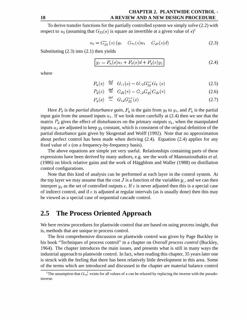
To derivetransferfunctionsfor thepartiallycontrolledsystemwesimplysolve(2.2)withrespectto $ � (assumingthat ��� )LI . is squareaninvertibleat agivenvalueof I )1
$ � % PO ���� )LI . ) # � 0 �A� )7I .;$ � 0 QB � )7I .;!/. (2.3)
Substituting(2.3) into (2.1) thenyields# � % �,R )LI .;$ �KJS� B )LI .N! JS�UT )7I .V# � (2.4)
where �,R )LI .XWZY\[% ��� )7I . 0 ��� O ���� �A� )LI . (2.5)� B )LI .XWZY\[% QB � )7I . 0 ��� O ���� QB � )7I . (2.6)�UT )LI .XWZY\[% ��� O ���� )LI . (2.7)
Here� B is thepartial disturbancegain,
�UTis thegainfrom # � to # � , and
�URis thepartial
input gainfrom theunusedinputs $ � . If we look morecarefullyat (2.4) thenweseethatthematrix
� B givestheeffect of disturbanceson theprimaryoutputs# � , whenthemanipulatedinputs $ � areadjustedto keep# � constant,whichis consistentof theoriginaldefinitionof thepartialdisturbancegaingivenby SkogestadandWolff (1992). Note thatno approximationaboutperfectcontrol hasbeenmadewhenderiving (2.4). Equation(2.4) appliesfor anyfixedvalueof I (on a frequency-by-frequency basis).
Theabove equationsaresimpleyet very useful. Relationshipscontainingpartsof theseexpressionshavebeenderivedby many authors,e.g.seethework of Manousiouthakisetal.(1986)on block relative gainsandthework of HaggblomandWaller (1988)on distillationcontrolconfigurations.
Notethat this kind of analysiscanbeperformedat eachlayer in thecontrolsystem.Atthetop layerwemayassumethatthecost is a functionof thevariables# � , andwecantheninterpret# � asthesetof controlledoutputs� . If � is neveradjustedthenthis is aspecialcaseof indirectcontrol,andif � is adjustedat regular intervals(asis usuallydone)thenthis maybeviewedasaspecialcaseof sequentialcascadecontrol.
2.5 The ProcessOriented Approach
Weherereview proceduresfor plantwidecontrolthatarebasedonusingprocessinsight,thatis, methodsthatareuniqueto processcontrol.
Thefirst comprehensive discussionon plantwidecontrolwasgivenby PageBuckley inhis book“Techniquesof processcontrol” in a chapteron Overall processcontrol (Buckley,1964). Thechapterintroducesthemain issues,andpresentswhat is still in many waystheindustrialapproachto plantwidecontrol. In fact,whenreadingthischapter, 35yearslateroneis struckwith thefeelingthattherehasbeenrelatively little developmentin this area.Someof thetermswhich areintroducedanddiscussedin thechapterarematerialbalancecontrol
1Theassumptionthat ]_^a`bLb existsfor all valuesof c canberelaxedby replacingtheinversewith thepseudo-inverse.
2.5. THE PROCESSORIENTED APPROACH 19
(in directionof flow, andin directionoppositeof flow), productionratecontrol,buffer tanksaslow-passfilters, indirect control, andpredictive optimization. He alsodiscussesrecycleandtheneedto purgeimpurities,andhepointsout thatyoucannotatagivenpoint in aplantcontrol inventory(level, pressure)andflow independentlysincethey arerelatedthroughthematerialbalance.In summary, hepresentsanumberof usefulengineeringinsights,but thereis really no overall procedure.As pointedout by Ogunnaike (1995) the basicprinciplesappliedby theindustrydoesnotdeviatefar from Buckley (1964).
Wolff andSkogestad(1994)review previouswork onplantwidecontrolwith emphasisontheprocess-orienteddecompositionapproaches.They suggestthatplantwidecontrolsystemdesignshouldstart with a “top-down” selectionof controlledand manipulatedvariables,andproceedwith a “bottom-up” designof the control system.At the endof the papertenheuristicguidelinesfor plantwidecontrolarelisted.
Thereexistsothermoreor lessheuristicsrulesfor processcontrol;e.g. seeHougenandBrockmeier(1969)andSeborg et al. (1995).
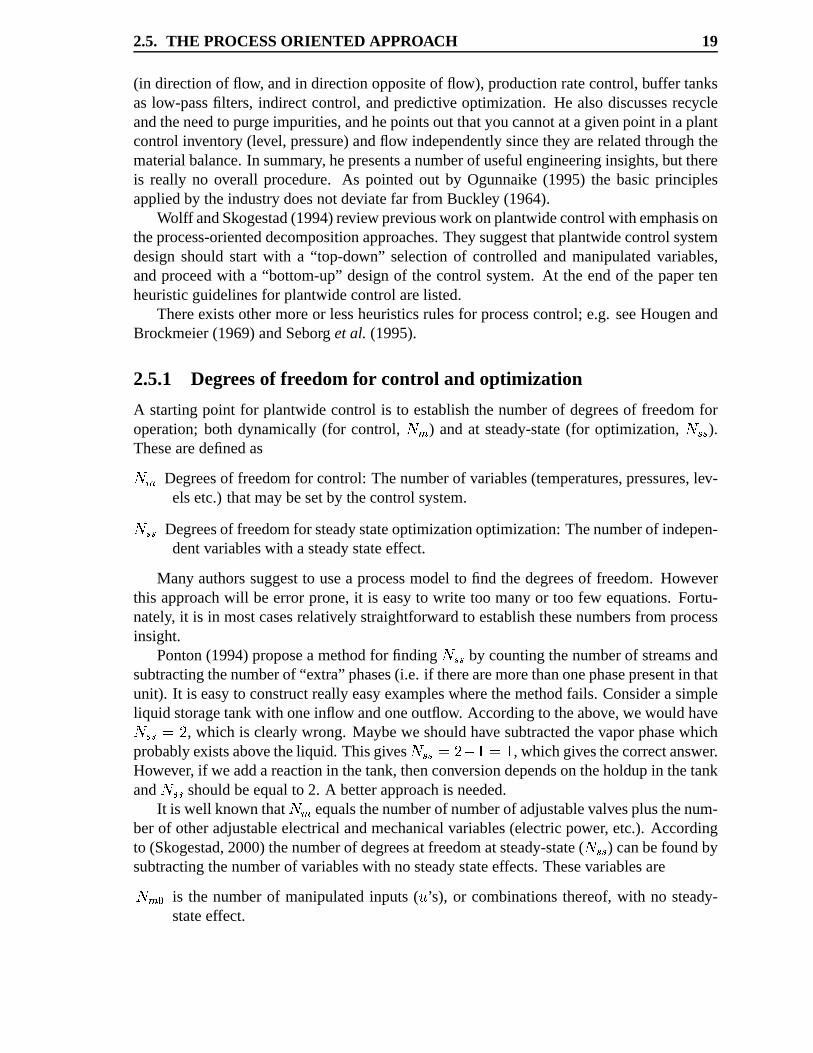
2.5.1 Degreesof fr eedomfor control and optimization
A startingpoint for plantwidecontrol is to establishthenumberof degreesof freedomforoperation;both dynamically(for control, d F ) andat steady-state(for optimization, d �L� ).Thesearedefinedasd F Degreesof freedomfor control: Thenumberof variables(temperatures,pressures,lev-
elsetc.) thatmaybesetby thecontrolsystem.d �7� Degreesof freedomfor steadystateoptimizationoptimization:Thenumberof indepen-dentvariableswith asteadystateeffect.
Many authorssuggestto usea processmodelto find thedegreesof freedom.Howeverthis approachwill beerrorprone,it is easyto write too many or too few equations.Fortu-nately, it is in mostcasesrelatively straightforwardto establishthesenumbersfrom processinsight.
Ponton(1994)proposea methodfor finding d �7� by countingthenumberof streamsandsubtractingthenumberof “extra” phases(i.e. if therearemorethanonephasepresentin thatunit). It is easyto constructreally easyexampleswherethemethodfails. Considera simpleliquid storagetankwith oneinflow andoneoutflow. Accordingto theabove,wewouldhaved �7�e%gf , which is clearlywrong. Maybewe shouldhave subtractedthevaporphasewhichprobablyexistsabovetheliquid. Thisgives d �L��%hf,0jik%li , whichgivesthecorrectanswer.However, if weaddareactionin thetank,thenconversiondependsontheholdupin thetankand d �7� shouldbeequalto 2. A betterapproachis needed.
It is well known that d F equalsthenumberof numberof adjustablevalvesplusthenum-berof otheradjustableelectricalandmechanicalvariables(electricpower, etc.). Accordingto (Skogestad,2000)thenumberof degreesat freedomatsteady-state( d �L� ) canbefoundbysubtractingthenumberof variableswith nosteadystateeffects.Thesevariablesared FMm is the numberof manipulatedinputs( $ ’s), or combinationsthereof,with no steady-
stateeffect.
20CHAPTER 2. PLANTWIDE CONTROL -
A REVIEW AND A NEW DESIGN PROCEDUREd TNm is thenumberof manipulatedinputsthatareusedto controlvariableswith no steady-stateeffect.
The latter usuallyequalsthe numberof liquid levels with no steady-stateeffect, includingmostbuffer tanklevels. However, notethatsomeliquid levelsdo have a steady-stateeffect,suchasthe level in a non-equilibriumliquid phasereactor, and levels associatedwith ad-justableheattransferareas.Also, we shouldnot includein d TAm any liquid holdupsthatareleft uncontrolled,suchasinternalstageholdupsin distillation columns.
Wefind that d TNm is nonzerofor mostchemicalprocesses,whereasweoftenhave d Fnm %o. A simpleexamplewhere d FMm is non-zerois a heatexchangerwith bypasson bothsides,
(i.e. d F %pf ). However, at steady-stated �7�1%qi sincethereis really only oneoperationaldegreeof freedom,namelytheheattransferrate r (which at steady-statemaybeachievedby many combinationsof thetwo bypasses),sowehave d FMm %li .
The optimizationis generallysubjectto several constraints.First, thereare generallyupperand lower limits on all manipulatedvariables(e.g. fully openor closedvalve). Inaddition,thereareconstraintson many dependentvariables;dueto safety(e.g. maximumpressureor temperature),equipmentlimitations (maximumthroughput)or productspecifi-cations. Someof theseconstraintswill be active at the optimum. The numberof “free”unconstrainedvariables“for steady-stateoptimization”, d �7�Vs tZu�v7v , is thenequaltod �L��s t-uGvLvw% d �L�M0 dyx;:\z|{~} vwhere dyx;:�z|{�} v is thenumberof active constraints.Notethat theterm“left for optimization”may be somewhat misleading,sincethe decisionto keepsomeconstraintsactive, reallyfollowsaspartof theoptimization;thusall d �L� variablesarereallyusedfor optimization.
Remarkon designdegreesof freedom. Above we have discussedoperationaldegreesof freedom. The designdegreeof freedom(which is not really a concernof this paper)includesall the d �7� operationaldegreesof freedomplusall parametersrelatedto thesizeoftheequipment,suchasthenumberof stagesin columnsections,areaof heatexchangers,etc.
Luyben(1996)claimsthat“designdegreesof freedomis equalto thenumberof controldegreesfor an importantclassof processes.” This is clearlynot true,asthereis no generalrelationshipbetweenthetwo numbers.For example,consideraheatexchangerbetweentwostreams.Then theremay be zero,one or two control degreesof freedom(dependingonthenumberof bypasses),but thereis alwaysonedesigndegreeof freedom(heatexchangerarea).
2.5.2 Production rate
Identifying the major disturbancesis very importantin any control problem,and for pro-cesscontrol the productionrate (throughput)is often the main disturbance. In addition,the locationof wherethe productionrate is actuallyset (“throughputmanipulator”),usu-ally determinesthe control structurefor the inventorycontrol of the variousunits. For aplant runningat maximumcapacity, the locationwheretheproductionrateis setis usuallysomewhereinside the plant, (e.g. causedby maximumcapacityof a heatexchangeror acompressor).Then,downstreamof this locationtheplanthasto processwhatever comesin
2.5. THE PROCESSORIENTED APPROACH 21
(givenfeedrate),andupstreamof this locationtheplanthasto producethedesiredquantity(givenproductrate).To avoid any “long loops”, it is preferablyto usetheinput flow for in-ventorycontrolupstreamthelocationwheretheproductionrateis set,andto usetheoutputflow for inventorycontroldownstreamthis location.
From this it follows that it is critical to know wherein the plant the productionrateisset. In practice,thelocationmayvary dependingon operatingconditions.This mayrequirereconfiguringof many control loops,but often supervisorycontrol systems,suchasmodelpredictivecontrol,providea simplerandbettersolution.
2.5.3 The framework of partial control and dominating variables
Shinnar(1981)introducedthefollowing setsof variablesS��� (the “primary” or “performance”or “economic” variables)is “the setof processvariablesthat definethe productand processspecificationsas well as processcon-straints”S� B is thesetof dynamicallymeasuredprocessvariablesS� :�B (a subsetof � B ) is the “set of processvariableson which we baseour dynamiccontrolstrategy”2� B is thedynamicinputvariables
The goal is to maintain �/� within prescribedlimits andto achieve this goal “we chooseinmostcasesa smallset � :�B andtry to keeptheseat a fixedsetof valuesby manipulating� B ”(later, in Arbel et al. (1996),heintroducedtheterm“partial control” to describethis idea).
Hewritesthattheoverallcontrolalgorithmcannormallybedecomposedinto adynamiccontrolsystem(which adjust � B ) anda steady-statecontrolwhich determinesthesetpointsof � :�B aswell asthevaluesof �n� [the latterarethemanipulationswhichonly canbechangedslowly], and that we “look for a set � :�B�+ � B that containsvariablesthat have a maximumcompensatingeffect on �/� ”. If onetranslatesthewordsandnotation,thenonerealizesthatShinnar’s ideaof “partial control” is very closeto theideaof “self-optimizingcontrol” pre-sentedin Morari et al. (1980),SkogestadandPostlethwaite (1996),andSkogestad(2000).Thedifferenceis thatShinnarassumesthat thereexist at theoutseta setof “primary” vari-ables��� thatneedto becontrolled,whereasin self-optimizingcontrolthestartingpoint is aneconomiccostfunctionthatshouldbeminimized.Theauthorsprovide someintuitive ideasandexamplesfor selectingdominantvariableswhichmaybeusefulin somecases,especiallywhennomodelinformationis available.
However, it is notclearhow helpful theideaof “dominant”variableis, sincethey arenotreally definedandno explicit procedureis givenfor identifying them. Indeed,Arbel et al.(1996)write that“the problemsof partialcontrolhavebeendiscussedin aheuristicway” andthat“considerablyfurtherresearchis neededto fully understandtheproblemsis steady-statecontrolof chemicalplants”.
22CHAPTER 2. PLANTWIDE CONTROL -
A REVIEW AND A NEW DESIGN PROCEDURE
Tyreus(1999b) provides someadditional interestingideason how to selectdominantvariables,partlybasedontheextensivevariableideaof Georgakis(1986)andthethermody-namicideasof Ydstie,(AlonsoandYdstie,1996),but againnoprocedurefor selectingsuchvariablesarepresented.
2.5.4 Decompositionof the problem
Thetaskof designingacontrolsystemfor completeplantsis alargeanddifficult task.There-fore mostmethodswill try to decomposetheprobleminto manageableparts.Four commonwaysof decomposingtheproblemare
1. Decompositionbasedonprocessunits
2. Decompositionbasedonprocessstructure
3. Decompositionbasedoncontrolobjectives(materialbalance,energy balance,quality,etc.)
4. Decompositionbasedon timescale
Thefirst is ahorizontal(decentralized)decompositionwhereasthelatterthreeprovidehierar-chicaldecompositions.Most practicalapproachescontainelementsfrom severalcategories.
Many of the methodsdescribedbelow performthe optimizationat the endof the pro-cedureafter checkingif therearedegreesof freedomleft. However, asdiscussedabove,it shouldbe possibleto identify the steady-statedegreesof freedominitially, andmake apreliminarychoiceoncontrolledoutputs( � ’s)beforegettinginto thedetaileddesign.
It is alsointerestingto seehow themethodsdiffer in termsof how importantinventory(level) control is considered.Someregard inventorycontrol as the most important(as isprobablycorrectwhenviewed purely from an operationalpoint of view) whereasPonton(1994)statesthat“inventoryshouldnormallyberegardedasthe leastimportantof all vari-ablesto beregulated”(which is correctwhenviewedfrom a designpoint of view). We feelthatthereis aneedto integratetheviewpointsof thecontrolanddesignpeople.
The unit basedapproach
Theunit-basedapproach,suggestedby Umedaet al. (1978),proposesto
1. Decomposetheplantinto individualunit of operations
2. Generatethebestcontrolstructurefor eachunit
3. Combineall thesestructuresto form acompleteonefor theentireplant.
4. Eliminate conflicts amongthe individual control structuresthrough mutual adjust-ments.
2.5. THE PROCESSORIENTED APPROACH 23
This approachhasalwaysbeenwidely usedin industry, andhasits mainadvantagethatmany effective control schemeshave beenestablishedover the yearsfor individual units(e.g.Shinskey (1988)).However, with anincreasinguseof materialrecycle,heatintegrationandthedesireto reducebuffer volumesbetweenunits,thisapproachmayresultin toomanyconflictsandbecomeimpractical.
As a result,onehasto shift to plantwidemethods,wherea hierarchicaldecompositionis used. The first suchapproachwasBuckley’s (1964)division of the control systemintomaterialbalancecontrolandproductquality control,andthreeplantwideapproachespartlybasedon his ideasaredescribedin thefollowing.
Hierar chical decompositionbasedon processstructure
Thehierarchygivenin Douglas(1988)for processdesignstartsatacruderepresentationandgetsmoredetailed:
Level 1 Batchvscontinuous
Level 2 Input-outputstructure
Level 3 Recyclestructure
Level 4 Generalstructureof separationsystem
Level 5 Energy interaction
Fisheret al. (1988a) proposeto usethis hierarchywhenperformingcontrollability analysis,andPontonandLaing (1993)point out that this hierarchy, (e.g. level 2 to level 5) couldalsobeusedfor controlsystemdesign.This framework enablesparalleldevelopmentfor theprocessandthecontrolsystem.Within eachof thelevelsaboveany designmethodmightbeapplied.
Ng andStephanopoulos(1998b) proposeto usea similar hierarchyfor controlstructuredesign.ThedifferencebetweenDouglas(1988)andNg andStephanopoulos(1998b)’shier-archyis that level 1 is replacedby a preliminaryanalysisandlevel 4 andon is replacedbymoreandmoredetailedstructures.At eachstepthe objectivesidentifiedat an earlierstepis translatedto this level andnew objectivesareidentified. The focusis on constructionofmassandenergy balancecontrol.Themethodis appliedto theTennesseeEastmancase.
All thesemethodshave in commonthat at eachlevel a key point is to checkif thereareenoughmanipulatedvariablesto meetthe constraintsand to optimizeoperation. Themethodsare easyto follow andgive a goodprocessunderstanding,and the conceptof ahierarchicalview is possibleto combinewith almostany designmethod.
Hierar chical decompositionbasedon control objectives
The hierarchybasedon control objectives is sometimescalled the tieredprocedure.Thisbottom-upprocedurefocuseson the tasksthat thecontrollerhasto perform. Normally onestartsby stabilizingthe plant, which mainly involvesplacinginventory(massandenergy)controllers.
24CHAPTER 2. PLANTWIDE CONTROL -
A REVIEW AND A NEW DESIGN PROCEDURE
Priceet al. (1993)build on the ideasthat wasintroducedby Buckley (1964)andtheyintroducea tieredframework. Theframework is dividedinto four differenttasks:
I Inventoryandproductionratecontrol.
II Productspecificationcontrol
III Equipment& operatingconstraints
IV Economicperformanceenhancement.
Their paperdoesnot discusspointsIII or IV. They performa largenumber(318)of simula-tionswith differentcontrolstructures,controllers(P or PI), andtuningson a simpleprocessconsistingof a reactor, separatorandrecycle of unreactedreactant.Theconfigurationsarerankedbasedon integratedabsoluteerrorof theproductcompositionfor stepsin thedistur-bance.Fromthesesimulationthey proposesomeguidelinesfor selectingthethroughputma-nipulatorandinventorycontrols.(1) Preferinternalflowsasthroughputmanipulator. (2) thethroughputmanipulatorandinventorycontrolsshouldbeself-consistent(self-consistency isfulfilled whenachangein thethroughputpropagatesthroughtheprocessby “itself ” anddoesnot dependon compositioncontrollers).They apply their ideason the TennesseeEastmanproblem(Priceet al., 1994).
Ricker (1996)commentsuponthe work of Priceet al. (1994). Ricker pointsout thatplantsareoftenrun at full capacity, correspondingto constraintsin oneor severalvariables.If a manipulatedvariablethat is usedfor level control saturates,one loosesa degreeoffreedomfor maximumproduction.This shouldbeconsideredwhenchoosinga throughputmanipulator.
Luybenet al. (1997)point out threelimitationsof theapproachof Buckley. First,hedidnot explicitly discussenergy management.Second,he did not look at recycles. Third, heplacedemphasison inventorycontrolbeforequalitycontrol.Their plantwidecontroldesignprocedureis listedbelow:
1. Establishcontrolobjectives.
2. Determinethe control degreesof freedomby countingthe numberof independentvalves.
3. Establishenergy inventorycontrol,for removing theheatsof reactionsandto preventpropagationof thermaldisturbances.
4. Setproductionrate. Theproductionratecanonly be increasedby increasingthe re-actionrate in the reactor. Onerecommendationis to usethe input to the separationsection.
5. Productquality andsafetycontrol.Herethey recommendtheusual“pair close”-rule.
6. Inventorycontrol.Fix aflow in all liquid recycle loops.They statethatall liquid levelsandgaspressuresshouldbecontrolled.
2.5. THE PROCESSORIENTED APPROACH 25
7. Checkcomponentbalances.(After thispoint it mightbeenecessaryto gobackto item4.)
8. Unit operationscontrol.
9. Optimizeeconomicsor improvedynamiccontrollability.
Step3 comesbeforedeterminingthe throughputmanipulator, sincethe reactoris typicallytheheartof theprocessandthemethodsfor heatremoval areintrinsicallypartof thereactordesign. In order to avoid recycling of disturbancesthey suggestto set a flow-rate in allrecyclesloops; this is discussedmorein section2.6. They suggestin step6 to control allinventories,but this may not be necessaryin all cases;e.g. it may be optimal to let thepressurefloat (Shinskey, 1988). They apply their procedureon several testproblems;thevinyl acetatemonomerprocess,theTennesseeEastmanprocess,andtheHDA process.
LarssonandSkogestad,in Chapter4, questionthe rule proposedby Luyben. By usingthesimplerecycle plant they areableto show thatapplicationof his rule may leadto largeproblem.
McAvoy (1999)presenta methodin which thecontrolobjective is dividedinto two cat-egories: variablesthat must be controlledandproductflow andquality. His approachisto find thesetof input thatwill minimizevalve movements,whereonly asmany valvesascontrolledvariablesareallowed to be used. This is first solved for the “must” variables,thenfor productrateandquality. Theoptimizationproblemis simplifiedby usinga linearstablesteadystatemodel. He givesno guidanceinto how to find which variablesthatmustbecontrolled.
Hierar chical decompositionbasedon time scales
Buckley (1964)proposedto designthequality controlsystemashigh-passfilters for distur-bancesandto designthe massbalancecontrol systemaslow passfilters. If the resonancefrequency of thequality controlsystemis designedto beanorderof magnitudehigherthanthebreakfrequency of themassbalancesystemthenthetwo loopswill benon-interacting.
McAvoy andYe(1994)divide their methodinto four stages:
1. Designof innercascadeloops.
2. Designof basicdecentralizedloops,exceptthoseassociatedwith quality andproduc-tion rate.
3. Productionrateandquality controls.
4. Higherlayercontrols.
The decompositionin stages1-3 is basedon the speedof the loops. In stage1 the ideaisto locally reducetheeffect of disturbances.In stage2 theregenerallyarea largenumberofalternative configurations.Thesemay be screenedusingsimplecontrollability tools, suchastheRGA. Oneproblemof selectingoutputsbasedona controllability analysisis thatone
26CHAPTER 2. PLANTWIDE CONTROL -
A REVIEW AND A NEW DESIGN PROCEDURE
mayendup with theoutputsthatareeasyto control,ratherthantheonesthatareimportantto control.Themethodis appliedto theTennesseeEastmantestproblem.
Douglas(1988),at page414, presentsa hierarchyfor control systemdesign,basedonthe dynamicsthat areinvolved. In this hierarchythe viewpoint is not on theflowsheetbuton steady-state,normaldynamicresponseandabnormaldynamicoperation. Zhenget al.(1999)continuethiswork. They placesagreaterattentionto feasibilityof theconstraintsandrobustoptimality (self-optimizingcontrol). In additionthey proposesto useminimumsurgecapacityasadynamiccost,(ZhengandMahajannam,1999).They havenotdocumentedthatthis will capturethetruedynamiccost.
2.6 The reactor, separatorand recycleplant
A commonfeatureof mostplantsis thepresenceof recycle. A simpleexampleis distillation,with recycle (“reflux”) of liquid from thetopof thecolumnandof vaporfrom thebottomofthecolumn.
In this section,we considerthe reactorand separatorprocesswith recycle of unre-actedfeed from a reactor. This kind of problem has lately beenstudiedby many au-thors,(Papadourakiset al., 1987),(Wolff et al., 1992),(Priceet al., 1993),(Luyben,1994),(Luyben and Floudas,1994), (Mizsey and Kalmar, 1996), (Wu and Yu, 1996), (Hansen,1998),(Ng andStephanopoulos,1998a), LarssonandSkogestad(in Chapter4) andmanymore.It maybedifficult to follow all thedetailsin thecasestudiespresented,soinsteadweaim in this sectionto gainsomebasicinsightinto theproblem.
In the simplestcase,let the reactorbe a CSTRwherecomponentA is convertedto aproductandtheamountconvertedis givenby� %h������� � ����������8 I��The amountof unreactedA is separatedfrom the productandrecycled backto the reactor(for simplicity we will hereassumeperfectseparation).To increasethe conversion
�one
thenhasthreeoptions:
1. Increasethetemperaturewhich increasesthereactionrateconstant� .2. Increasethe amountof recycle, which indirectly increasesthe fraction of A in the
reactor, ��� .
3. Increasethereactorholdup � . (In a liquid phasesystemthereactorholdupis deter-minedby thereactorlevel, andin a gasphasesystemby thereactorpressure.)
Herewewill assumethatthetemperatureis constant,sotherearetwo optionsleft.Sinceat steady-statewith givenproductspecificationstheconversionof A in thereactor
is givenby the feedrate,it follows thatonly oneof the two remainingoptionscanbecon-trolled independently(or moregenerally, onevariablethatinfluencestheseoptions),andwemustlet thesecondvariable”float” andadjustitself.
Two commoncontrolstrategiesarethen
2.6. THE REACTOR, SEPARATOR AND RECYCLE PLANT 27
(A) Controlthereactorholdup(andlet therecycleflow float)
(B) Controltherecycleflow (andlet thereactorholdupfloat).
In case(A) onemay encounterthe so-called”snowball effect” wherethe recycle goestoinfinity. Thisoccursbecauseat infinite recycleflow wehave ���&%li whichgivesthehighestpossibleproduction.In effect, thesnowball effect occursbecausethereactoris too small tohandlethegivenfeedrate,soit is really asteady-statedesignproblem.
Luyben(1992,1994)hasstudiedliquid phasesystemsandhasconcludedthat controlstrategy (B) (or a variantof it) with oneflow fixed in the recycle loop shouldbe usedtoavoid the”snowball effect”.
Wu andYu (1996)alsostudy the snowball effect for the reactor/separatorandrecycleplant. They proposeas a remedyto the snowball effect to distribute the “work” evenlybetweenthedifferentunits.To achieve this they suggestto
(C) Controlthereactorcompositionconstant.
Also in this casethereactorvolumevariesdependingon thedisturbance.
However, from an economicpoint of view oneshouldusuallyfor liquid phasesystemskeepthereactorlevel at its maximumvalue,Chapter4. This maximizestheconversionperpassandresultsin thesmallestpossiblerecycle,whichgenerallywill reducetheoperationalcost. Thus, the recommendationof Luyben(1992,1994)and(Wu andYu, 1996),hasaneconomicpenaltywhich it seemsthatmostresearcherssofar haveneglected.
On the other hand,for gasphasesystems,thereis usually an economicpenaltyfromcompressioncostsinvolvedin increasingthereactorholdup(i.e. the reactorpressure),andstrategy (B) wherewe let the holdup(pressure)float may in fact be optimal. Indeed,suchschemesareusedin industry, e.g. in ammoniaplants.For example,for processeswith gasrecycle andpurge,Fisheret al. (1988a) recommendto keepthegasrecycle constantat themaximumvalue.For a simplegasphaseplantandtherecycle plantwe have shown thattheeconomicoptimumdoesnotcoincidewith themaximumrecycleflow, Chapter5.
Wolff etal. (1992)studiedasimilarplant.They includedaninertcomponentandlookedon the effectsof recycle on the controllability of the process.Their conclusionis that thepurgestreamflow shouldbeusedto controlthecompositionof inert. They did not considerthereactorholdupasapossiblecontrolledvariable.
All the above works have in commonthat the authorsaresearchingfor the right con-trolledvariablesto keepconstant(recycleflow, reactorvolume,composition,etc.).However,acommonbasisfor comparingthealternativesseemsto belacking. In termsof futurework,weproposethatonefirst needsto defineclearlytheobjectivefunction(cost) for theopera-tion of thereactorsystem.Only whenthis is given,mayonedecidein a rigorousmanneronthebestselectionof controlledoutputs,for exampleby usingthe ideaof “self-optimizing”controlandevaluatingtheloss.This is donein asystematicmannerChapter4 and5.
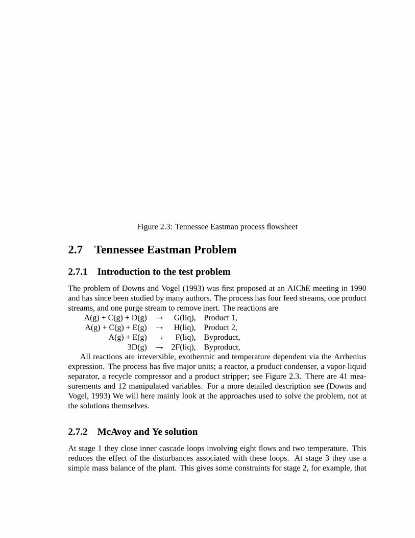
28CHAPTER 2. PLANTWIDE CONTROL -
A REVIEW AND A NEW DESIGN PROCEDURE
Stm
FI
TI
Reactor
TIFI
XA
XB
XC
XD
XF
XE
E
D
A
SC
LI
CWS
CWR
CWS
CWR
TI
FI
C
Cond
Product
FI
TI
LI
FI
Purge
FI
PI
JI Compressor
XA
XB
XC
XD
XF
XE
XG
XH
XD
XF
XE
ANALYZER
XG
XH
Vap/Liq
StripperSeparator
Condenser
1
2
3
6
4
7
12
5
8
10
11
9
LI
PI
FI
FI
FI
FI
ANALYZER
ANALYZER
PI
TI
y1
y2
y3
y4
u4
u2
u1
u3
y6
y8
u12
y7
y21
y9
u10
u11
y22
y20
y5 u5
y10
u6
y13
y12
y11y14
u7
y18
y16
y15
y17
u8
u9
y19
y3
y23
y24
y25
y26
y27
y28
y29
y30
y31
y32
y33
y34
y35
y36
y37
y38
y39
y40
y41
(y1)(y2)
(y3)
(y4)
(y5)(y6)
(y7)
(y8)
(y9)
(y10)
(y11)
Figure2.3: TennesseeEastmanprocessflowsheet
2.7 TennesseeEastmanProblem
2.7.1 Intr oduction to the testproblem
Theproblemof DownsandVogel (1993)wasfirst proposedat anAIChE meetingin 1990andhassincebeenstudiedby many authors.Theprocesshasfour feedstreams,oneproductstreams,andonepurgestreamto removeinert. Thereactionsare
A(g) + C(g) + D(g) � G(liq), Product1,A(g) + C(g)+ E(g) � H(liq), Product2,
A(g) + E(g) � F(liq), Byproduct,3D(g) � 2F(liq), Byproduct,
All reactionsareirreversible,exothermicandtemperaturedependentvia the Arrheniusexpression.Theprocesshasfive majorunits;a reactor, a productcondenser, a vapor-liquidseparator, a recycle compressoranda productstripper;seeFigure2.3. Thereare41 mea-surementsand12 manipulatedvariables.For a moredetaileddescriptionsee(Downs andVogel,1993)We will heremainly look at theapproachesusedto solve theproblem,not atthesolutionsthemselves.
2.7.2 McAvoy and Yesolution
At stage1 they closeinner cascadeloopsinvolving eightflows andtwo temperature.Thisreducesthe effect of the disturbancesassociatedwith theseloops. At stage3 they useasimplemassbalanceof theplant. This givessomeconstraintsfor stage2, for example,that
2.7. TENNESSEEEASTMAN PROBLEM 29
eithertheC-feedor theproductflow mustbeleft for thethird stage.At stage2 decentralizedloopsareclosed.They startwith the level loopssincethey are
the most importantloops. Therearethreelevel loops; reactor, separatorandstripper, andthey considerfour possiblelevel configurations.Threeof theconfigurationswereruledoutbasedon controllability analysis.Thealternative wheretheE-feedis usedfor reactorlevelcontrol is analyzedin greaterdetail. They look at three ����� , eighteen����� , andfifteen ���*�systems,wherethecontrolledoutputsseemto beratherrandomlychosen.After ananalysisinvolving RGA,Niederlinskiindex andlinearvalvesaturation,only four alternativesareleft.Thesearefurtherscreenedon their steady-statebehavior for a rangeof disturbances.
2.7.3 Lyman, Georgakis and Price’s solution
Georgakisandcoworkershavestudiedtheproblemin severalpapers(LymanandGeorgakis,1995),(Priceetal., 1994).They startby identifying theprimarypath,which is from therawmaterials,throughthereactor, condenser, thestripper, andto theproductflow. They do notconsiderthe C-feedsinceit is in excessin the recycle. In (Priceet al., 1994)they list allcandidatesfor throughputmanipulationsalongtheprimarypath: Thefeedstreams,flow ofcoolantto reactorcondenser, theseparatordrumbottomsflowsandfinal productflow. Of thefeedsonly D is considered.TheC-feedwasnotacandidateasthroughputmanipulatorsinceit wasassumednot to beon theprimarypath.Next, they list theinventoriesthatneedto becontrolled:pressure,reactorlevel, separatorlevel andstripperlevel. Inventorycontrolsarechosensoto constructaself-consistentpath(which doesnot dependon qualitycontrollers).At thispoint they havefour differentstructures.After thisreactortemperaturecontrollerandquality controllersareadded.
Theirprocedureis simpleandclearto follow. Theresultis acontrolsystemthatis fairlysimpleto understand.
2.7.4 Ricker’s solution
Ricker (1996)startsby listing the variablesthatmustbe controlled: productionrate,mole% G in product, reactorpressure,reactorliquid level, separatorlevel and stripper level.The productionrate is chosenas the input that most likely is going to saturate;namelyacombinationof D andE. Theremainingcontrolsystemfollows by applyingquality controlandinventorycontrol.After thatoverridesareinstalled.
2.7.5 Luyben’s solution
Luybenetal. (1997)look ontwocases,controlof throughputwith theproductflow orcontrolwith the A-feed. Herewe only look at the casewherethe productflow is the throughputmanipulator. At step3 they look at energy inventorycontrol,which in this caseis to controlthereactortemperaturewith thereactorcoolingwater. In step5 they assignthestrippersteamstreamto control strippertemperature,andthereforealsothe productcompositions.Sincethe pressureof the reactormustbe kept within bounds,they usethe largestgasfeed(thefeedof C) to controlthereactorpressure.Step7 is thecheckof componentbalances,which
30CHAPTER 2. PLANTWIDE CONTROL -
A REVIEW AND A NEW DESIGN PROCEDURE
givesacompositioncontrollerfor inertusingthepurgeflow andacompositioncontrollerforA usingthe A-feed. After doing somesimulationsthey adda controllerfor control of thecondenser, usingthereactortemperature.
Theresultingcontrolsystemis simple,but therecouldhavebeenabetterjustificationonwhatoutputsto control.
2.7.6 Ng and Stephanopulos’s solution
Ng andStephanopoulos(1997,1998)startby stabilizingthereactor. Thenthey proceedtolook at the input/outputlevel of the plant, wherethe centralpoint is to fulfill materialandenergy balances.At this level it shouldhave beenpossibleto saysomethingabouthow thefeedsshouldbeadjustedin orderto achievetheright mix of G andH, but they donot. Ratherthey look atwhichfeedor exit flowsthatshouldbeusedto maintainmaterialbalancecontrol.
At the final level they translatethe control objectivesto measurements.Herematerialbalancecontrol is translatedinto inventorycontrollers,like productflow to controlstripperlevel andbottomflow to controlseparatorlevel. Thenext objective is thenreactorpressurewherepurge is assigned.Finally feed E is assignedto control of productratio, andE isassignedto throughputcontrol. TheA andC feedis usedfor controllingcompositionof AandC.
The methodis somewhatdifficult to follow andthey seemto repeatmany of the argu-mentsin eachphase.
2.7.7 Larsson,Hestetunand Skogestad’ssolution
Larsson,HestetunandSkogestad(in Chapter6) usestheconceptof self-optimizingcontrolfor selectingthecontrolledvariables.This problemis well suitedsincetheeconomicobjec-tivewasdefined.Howeverthisproblemis largerin size,andthey needsto useprocessinsightto reducethenumberof alternative structures.For example,they chooseto control reactortemperaturesinceeverybodyelsedoesit. Still they manageto comeup with a solutionwithgoodself-optimizingproperties.
2.7.8 Other work
The above review is by no meanscomplete,andtherearemany authorswho have workedon this problem,someare(Wu andYu, 1997),(BanerjeeandArkun, 1995)and(Scali andCortonesi,1995). In additionthereareseveralothersthathaslookedat otheraspectsof theTennesseeEastmanplant.
2.7.9 Other testproblems
Thereareseveralothertestproblem,thataresuitablefor studyingissuesrelatedto plantwidecontrol. TheseincludetheHDA-plant (Douglas,1988),thevinyl acetatemonomerprocess(LuybenandTyreus,1998),therecycleplant(Wu andYu,1996)andtheLuybenandLuybenplant(LuybenandLuyben,1995).
2.8. A NEW PLANTWIDE CONTROL DESIGN PROCEDURE 31
2.8 A newplantwide control designprocedure
Basedthe above review andasa conclusionto this paper, we proposea plantwidedesignprocedure.The proceduremainly follows the mathematicallyorientedapproach,but withsomeelementsfrom theprocessorientedapproach.We proposeto first performa top-downanalysisto selectcontrolledvariables,basedontheideasof self-optimizingcontrol.For thiswe needa steadystatemodelandoperationalobjectives(steadystateeconomics).Theresultis oneor morealternativesetsfor (primary)controlledvariables( # � %�� . .
This top-down analysisis followed by a bottom-upassignmentandpossiblydesignofthecontrol loops. This is donein a sequentialmannerstartingwith stabilization.Next weconsiderthe fast loopsneededfor local disturbancerejection. Herewe may make useof(extra) secondarymeasurements( # � ). This is the “regulatory” control layer (system).Theobjective for theregulatorylayeris thatmanualoperationof theplantis possibleaftertheseloopsareclosed.
We now have asdegreesof freedomthe setpointsof the regulatorylayer ( ' � ) plus anyunusedmanipulators( $ � ), theseshouldbe usedto control the primary outputs( # � ). Thiscontrol layer is often called the supervisorycontrol layer. This namemay be misleadingor too limited. Oftena supervisorycontrolleris only “activated”whensomethinghasgonewrong(e.g. logical switches),but we will alsouseit for “active” controllers.An alternativenamecouldhave beenadvancedcontrol layer, but advancedis a relative word andit is notgiventhatthecontrollersin this layerareadvanced.
Therearetwo mainapproacheshere:Useof singleloop (decentralized)controllerswithpossiblefeed-forward links, or useof multivariablecontrol,e.g. decouplingor modelpre-dictivecontrol(MPC).Properlydesignedmultivariablecontrollersgivebetterperformance,but this mustbetradedagainstthecostof obtainingandmaintainingthemodelsusedin thecontroller.
Themainresultof thiswill bethecontrolstructure,but controllertuningmayalsobeob-tained.Finally, nonlineardynamicsimulationsshouldbeperformedto validatetheproposedcontrolstructure.
2.9 Conclusion
In this paperwe have givena review on plantwidecontrol with emphasison the followingtasksthatmakeup thecontrolstructuredesignproblem:
1. Selectionof controlledoutputs( � with setpoints��� ).2. Selectionof manipulatedinputs( � ).
3. Selectionof measurements( � )4. Selectionof control configuration
5. Selectionof controller type
32CHAPTER 2. PLANTWIDE CONTROL -
A REVIEW AND A NEW DESIGN PROCEDURE
Themainemphasishasbeenon theselectionof controlledoutputs,wherewe have seenthat theuseof a steady-stateeconomiccriterion is very useful. It appearsthat thesolutionto this taskprovidesthe muchneededlink betweensteady-stateoptimizationandprocesscontrol, and that the idea of “self-optimizing control” to reducethe effect of uncertaintyprovidesa very usefulframework for makingthe right decision.We thusproposethat thedesignof thecontrolsystemshouldstartwith theoptimization(or at leastidentifying whatthecontrolobjectivesreallyare)andthusproviding candidatesetsfor thecontrolledoutputs.Thecontrolproblemis thendefined,andonemayproceedto analyze(e.g. usingan input-outputcontrollabilityanalysis,whetherthecontrolobjectivescanbemet).
The actualdesignof the control systemis doneat the end, after the control problemhasbeendefined,includingtheclassificationof all variables(into inputs,disturbances,con-trolled variables,etc.). Control systemdesignusuallystartswith stabilizingcontrol whereit is usually importantto avoid input saturation.The control systemis thenbuild up in ahierarchicalmannersuchthat eachcontrolleris of limited size(usuallywith asfew inputsandoutputsaspossible).Emphasisshouldbeon avoiding “long” loops,that is, oneshouldpair inputsandoutputswith are“close” to another.
Mostof theproposedprocessorientedprocedureshaveelementsfrom thiswayof think-ing,althoughsomeproceduresfocusmostlyoncontrolandoperationandseemto skiplightlyover thephasewheretheoverallcontrolproblemis defined.
Severalcasestudieshave beenproposed,which is good.However, someof thework onthesecasestudiesseemsto provide little generalinsight, andtheir valuemay thereforebequestioned.A moresystematicapproachandacommongroundof comparisonaresuggestedfor futurework.
In summary, thefield of plantwidecontrol is still at a relatively earlystageof its devel-opment. However, the progressover the last few years,both in termsof casestudiesandtheoreticalwork, bearspromisefor thefuture.Thereis still aneedfor aclearerdefinitionofthe issues,andit is hopedthat this papermaybeusefulin this respect.In the longerterm,whereautomaticgenerationandanalysisof alternativestructuresmaybecomemoreroutine,themainproblemwill probablybeto beableto generatemodelsin anefficient way, andtoprovideefficientmeansfor their analysis(e.g.usinginput-outputcontrollability analysis).
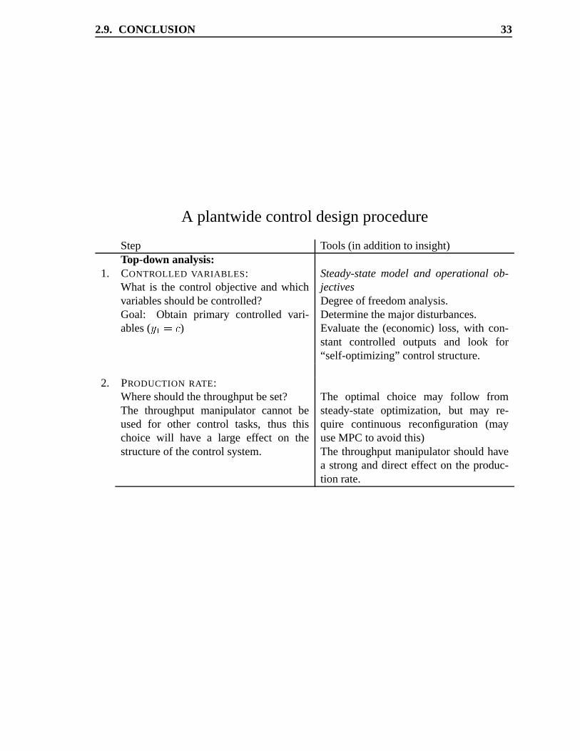
2.9. CONCLUSION 33
A plantwidecontroldesignprocedure
Step Tools(in additionto insight)Top-down analysis:
1. CONTROLLED VARIABLES:What is the control objective andwhichvariablesshouldbecontrolled?Goal: Obtain primary controlled vari-ables( # � % � )
Steady-statemodel and operational ob-jectivesDegreeof freedomanalysis.Determinethemajordisturbances.Evaluatethe (economic)loss, with con-stant controlled outputs and look for“self-optimizing” controlstructure.
2. PRODUCTION RATE:Whereshouldthethroughputbeset?The throughput manipulator cannot beused for other control tasks, thus thischoice will have a large effect on thestructureof thecontrolsystem.
The optimal choice may follow fromsteady-stateoptimization, but may re-quire continuous reconfiguration (mayuseMPC to avoid this)The throughputmanipulatorshouldhavea stronganddirect effect on the produc-tion rate.
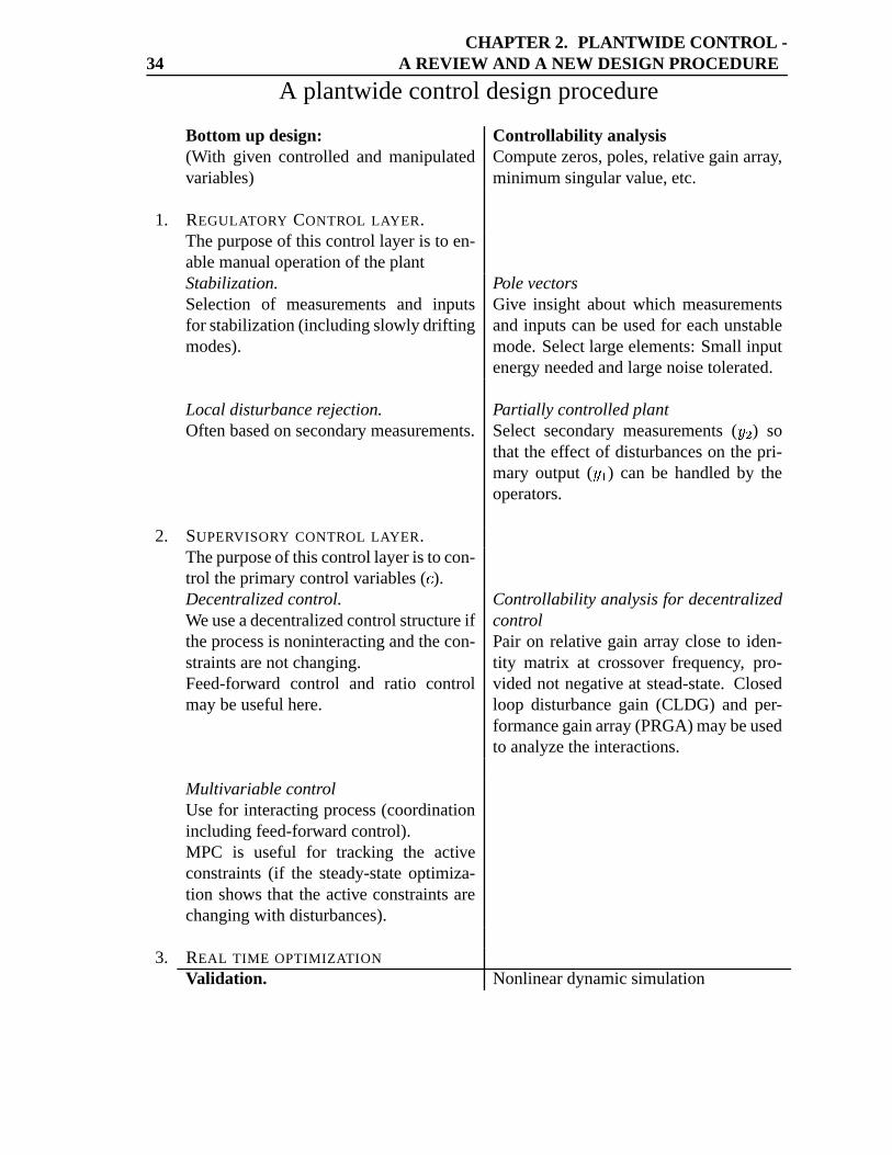
34CHAPTER 2. PLANTWIDE CONTROL -
A REVIEW AND A NEW DESIGN PROCEDURE
A plantwidecontroldesignprocedure
Bottom up design:(With given controlled and manipulatedvariables)
Controllability analysisComputezeros,poles,relativegainarray,minimumsingularvalue,etc.
1. REGULATORY CONTROL LAYER.Thepurposeof this controllayeris to en-ablemanualoperationof theplantStabilization.Selection of measurementsand inputsfor stabilization(includingslowly driftingmodes).
PolevectorsGive insight aboutwhich measurementsandinputscanbe usedfor eachunstablemode.Selectlargeelements:Small inputenergy neededandlargenoisetolerated.
Localdisturbancerejection.Oftenbasedonsecondarymeasurements.
Partially controlledplantSelect secondarymeasurements( # � ) sothat theeffect of disturbanceson thepri-mary output ( # � ) can be handledby theoperators.
2. SUPERVISORY CONTROL LAYER.Thepurposeof thiscontrollayeris to con-trol theprimarycontrolvariables( � ).Decentralizedcontrol.Weuseadecentralizedcontrolstructureiftheprocessis noninteractingandthecon-straintsarenotchanging.Feed-forward control and ratio controlmaybeusefulhere.
Controllability analysisfor decentralizedcontrolPair on relative gain arraycloseto iden-tity matrix at crossover frequency, pro-vided not negative at stead-state.Closedloop disturbancegain (CLDG) and per-formancegainarray(PRGA)maybeusedto analyzetheinteractions.
MultivariablecontrolUsefor interactingprocess(coordinationincludingfeed-forwardcontrol).MPC is useful for tracking the activeconstraints(if the steady-stateoptimiza-tion shows that the active constraintsarechangingwith disturbances).
3. REAL TIME OPTIMIZATION
Validation. Nonlineardynamicsimulation
Chapter 3
Limitations imposedbylower layer partial control
T. LarssonandS.Skogestad
Extendedversionof paperpresentedat AIChE Annualmeeting1998,Miami.
Abstract
In thischapterwestudyhow fundamentallimitationscanbeintroducedby improperdesignof thelowercontrollayer. Oneusefultool for analyzingthis problemis theconceptof partialcontrol,which shows how theplantlooksasseenfrom thehigherlayercontroller.
Theconclusionis thatwe cannotintroducenew limitations,providedthatwe have accessto themeasure-mentsof the alreadyclosedloops,that their setpointsareavailableasdegreesof freedomandthat the lowerlayercontrolleris stableandminimumphase.
However, in somecasesthe requirementsarenot met,andwe may introducelimitations. For exampleif
the setpointsof the lower layer areunavailable,pairing on a negative RGA may introducea negative RHP-
zero (inverseresponse)in the remainingsystem. We may also introducesensitivity to disturbancesand ill-
conditioninginto theremainingsystem.
36CHAPTER 3. LIMIT ATIONS IMPOSED BY
LOWER LAYER PARTIAL CONTROL
3.1 Intr oduction
A hierarchicalcontrolsystemariseswhendesignis donein a sequentialmanner. Typically,a chemicalplant hasat leastthreelayers;a regulatory (base)control layer, a supervisorycontrollayerwith localoptimization(e.g.modelpredictivecontrol),andanoptimizinglayer(usuallybasedonsteady-stateoptimization).Thefunctionsin thetwo upperlayersareoftenperformedbyhumans.Thelowerregulatorycontrollayerusuallyconsistsof PID controllers.Thetaskof this layeris to “stabilize” theplant,sothat it canbeoperatedmanually, withoutthehigh level controllersin place.
Hovd andSkogestad(1993)proposedsomerulesfor designingthe lower layer. Oneofthe pointsthey mentionis that oneshouldnot introducenew fundamentallimitations, likeRHP-zerosandill-conditioning,into theremainingcontrolproblem.Is thisreallyaproblem?That is, cananimproperselectionof thebasecontrol layer leadto unnecessarylimitations,whichcannotbeovercomeby thehigherlayers?By “unnecessary”wemeanlimitationsthatwerenotpresentasfundamentallimitationsin theoriginalplant.
The aim of this paperis to study this problemmore generally: Can we by improperdesignof a lower layercontrolsystem,introduce(new) fundamentallimitationsnot presentin theoriginal system?
We will usethe terms“lower layer” and“inner loop” assynonyms,andalsothe terms“upperlayer” and“outer loop” areusedassynonyms.Thetermfundamentallimitation willhereimply a restrictionon theattainablecontrolperformance.
Outline
We first introducethe ideaof partial control, andthendiscusshow to cancelthe effect ofthe lower control layer. We thendiscussthepossibility for RHP-zerosin subsystemsunderpartial control. Next we look at the effect of disturbanceunderpartial control,andthenatill-conditioning, asindicatedby large RGA elements.Finally oneexampleis devotedto ahigh-puritydistillationcolumn,whereit seemsthatwecanremovea fundamentallimitationby closingthelower layerlevels.
3.2 Partial Control
Oneusefultool for analyzingtheeffect of closinglower layer loops,is theconceptof par-tial control, e.g. (HaggblomandWaller, 1988), (SkogestadandWolff, 1992), (Havre andSkogestad,1996a) and(SkogestadandPostlethwaite,1996). We partition the inputs $ andoutputs# into two sets # %¢¡ # �# �¤£ +¥$ %¦¡ $ �$ �y£Thelinearmodel # % C$ J QB§! maythenbewritten# � % ��� $ �KJ ��� $ �nJ QB � ! (3.1)# � % �A� $ �KJ ��� $ �nJ QB � ! (3.2)
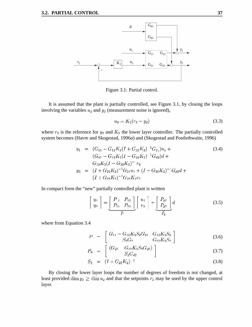
3.2. PARTIAL CONTROL 37
-
K
d G
G
G
G
u y
yur222
2 2
1
d1
d2
11 12
21 G
1
2
G
Figure3.1: Partial control.
It is assumedthat the plant is partially controlled,seeFigure3.1, by closingthe loopsinvolving thevariables$ � and # � (measurementnoiseis ignored),$ � % � � ) ' � 0 # � . (3.3)
where ' � is the referencefor # � and � � the lower layercontroller. Thepartially controlledsystembecomes(Havre andSkogestad,1996a) and(SkogestadandPostlethwaite,1996)# � % ) ��� 0 ��� � � )�¨ J ��� � � . O � �A� .V$ ��J (3.4)) CB � 0 ��� � � )�¨ J ��� � � . O � CB � .N! J ��� � � )�¨ J ��� � � .ZO � ' �# � % )�¨ J ��� � � .ZO � �A� $ �KJ )�¨ J ��� � � .-O � CB � ! J)�¨ J ��� � � .ZO � ��� � � ' �In compactform the“new” partially controlledplantis written¡ # �# � £ % ¡ �����©������U�A�©�U��� £ª «�¬ ® ¡ $ �' � £ J ¡ � B �� B � £ª «�¬ ®�¯ ! (3.5)
wherefrom Equation3.4� % ¡ ��� 0 ��� � �§°±� �A� ��� � �§°±�°±� �A� ��� � �§°±�¤£ (3.6)� B % ¡ ) QB � 0 ��� � �§°±� CB � .°±� CB � £ (3.7)°±� % )�¨ J ��� � � . O � (3.8)
By closingthe lower layer loopsthe numberof degreesof freedomis not changed,atleastprovided ²´³¶µS# �P· ²´³¶µS$ � andthat thesetpoints' � maybeusedby theuppercontrollayer.
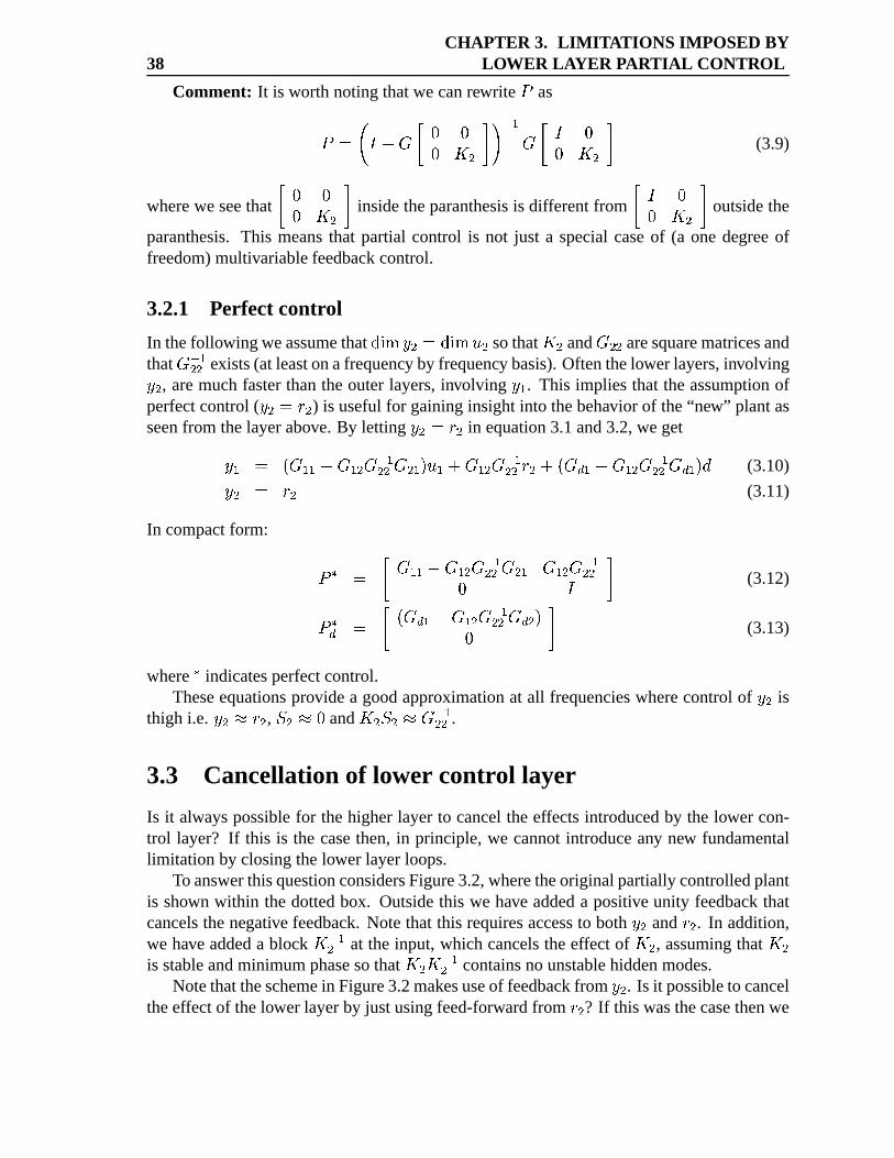
38CHAPTER 3. LIMIT ATIONS IMPOSED BY
LOWER LAYER PARTIAL CONTROL
Comment: It is worth notingthatwe canrewrite�
as� %X¸�¨ J ¡ o oo � � £�¹ O� ¡ ¨ oo � � £ (3.9)
wherewe seethat ¡ o oo � �¤£ insidetheparanthesisis differentfrom ¡ ¨ oo � �P£ outsidethe
paranthesis.This meansthat partial control is not just a specialcaseof (a onedegreeoffreedom)multivariablefeedbackcontrol.
3.2.1 Perfect control
In thefollowing weassumethat ²´³¶µS# � % ²´³ºµ»$ � sothat � � and ��� aresquarematricesandthat O ���� exists(at leastonafrequency by frequency basis).Oftenthelowerlayers,involving# � , aremuchfasterthantheouterlayers,involving # � . This implies that theassumptionofperfectcontrol( # � % ' � ) is usefulfor gaininginsightinto thebehavior of the“new” plantasseenfrom thelayerabove. By letting # � % ' � in equation3.1and3.2,weget# � % ) ��� 0 ��� O ���� �A� .;$ �KJ ��� O ���� ' �¼J ) CB � 0 ��� O ���� QB � .;! (3.10)# � % ' � (3.11)
In compactform: �Q½ % ¡ ��� 0 ��� ¾O ���� �A� ��� PO ����o ¨ £ (3.12)�Q½B % ¡ ) CB � 0 ��� O ���� QB � .o £ (3.13)
where½
indicatesperfectcontrol.Theseequationsprovide a goodapproximationat all frequencieswherecontrolof # � is
thigh i.e. # �_¿ ' � , °±�À¿ oand � ��°±�_¿ O ���� .
3.3 Cancellationof lower control layer
Is it alwayspossiblefor thehigherlayer to canceltheeffectsintroducedby the lower con-trol layer? If this is the casethen,in principle,we cannotintroduceany new fundamentallimitation by closingthelower layerloops.
To answerthisquestionconsidersFigure3.2,wheretheoriginalpartiallycontrolledplantis shown within thedottedbox. Outsidethis we have addeda positive unity feedbackthatcancelsthenegative feedback.Notethat this requiresaccessto both # � and ' � . In addition,we have addeda block �ÁO �� at the input, which cancelstheeffect of � � , assumingthat � �is stableandminimumphasesothat � � � O �� containsno unstablehiddenmodes.
Notethattheschemein Figure3.2makesuseof feedbackfrom # � . Is it possibleto canceltheeffectof thelower layerby justusingfeed-forwardfrom ' � ? If thiswasthecasethenwe
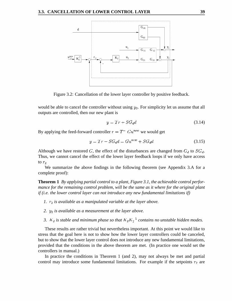
3.3. CANCELLA TION OF LOWER CONTROL LAYER 39
K2u2
-
G
uG
Gy
12
22
G
1
d1
d2
11
21 G
Gy
K2-1
2
1
2 2r
d
unew
Figure3.2: Cancellationof thelower layercontrollerby positive feedback.
would beableto cancelthecontrollerwithout using # � . For simplicity let usassumethatalloutputsarecontrolled,thenour new plantis# %2 ' Jð QB§! (3.14)
By applyingthefeed-forwardcontroller ' %Ä O � Q$ÆÅ v�Ç wewouldget# %2 ' Jð QB§! % C$ Å v7Ç Jð QB§! (3.15)
Althoughwe have restored , the effect of the disturbancesarechangedfrom CB to° QB .
Thus,we cannotcanceltheeffect of the lower layer feedbackloopsif we only have accessto ' �
We summarizethe above findings in the following theorem(seeAppendix 3.A for acompleteproof):
Theorem 1 Byapplyingpartial control to a plant,Figure3.1,theachievablecontrol perfor-mancefor theremainingcontrol problem,will bethesameasit where for theoriginal plantif (i.e. thelower control layercannot introduceanynew fundamentallimitationsif)
1. ' � is availableasa manipulatedvariableat thelayerabove.
2. # � is availableasa measurementat thelayerabove.
3. � � is stableandminimumphasesothat � � �ÁO �� containsnounstablehiddenmodes.
Theseresultsarerathertrivial but neverthelessimportant.At this point we would like tostressthat the goal hereis not to show how the lower layer controllerscould be canceled,but to show thatthelower layercontroldoesnot introduceany new fundamentallimitations,provided that the conditionsin the above theoremaremet. (In practiceonewould setthecontrollersin manual.)
In practicethe conditionsin Theorem1 (and 2), may not always be met and partialcontrol may introducesomefundamentallimitations. For exampleif the setpoints' � are
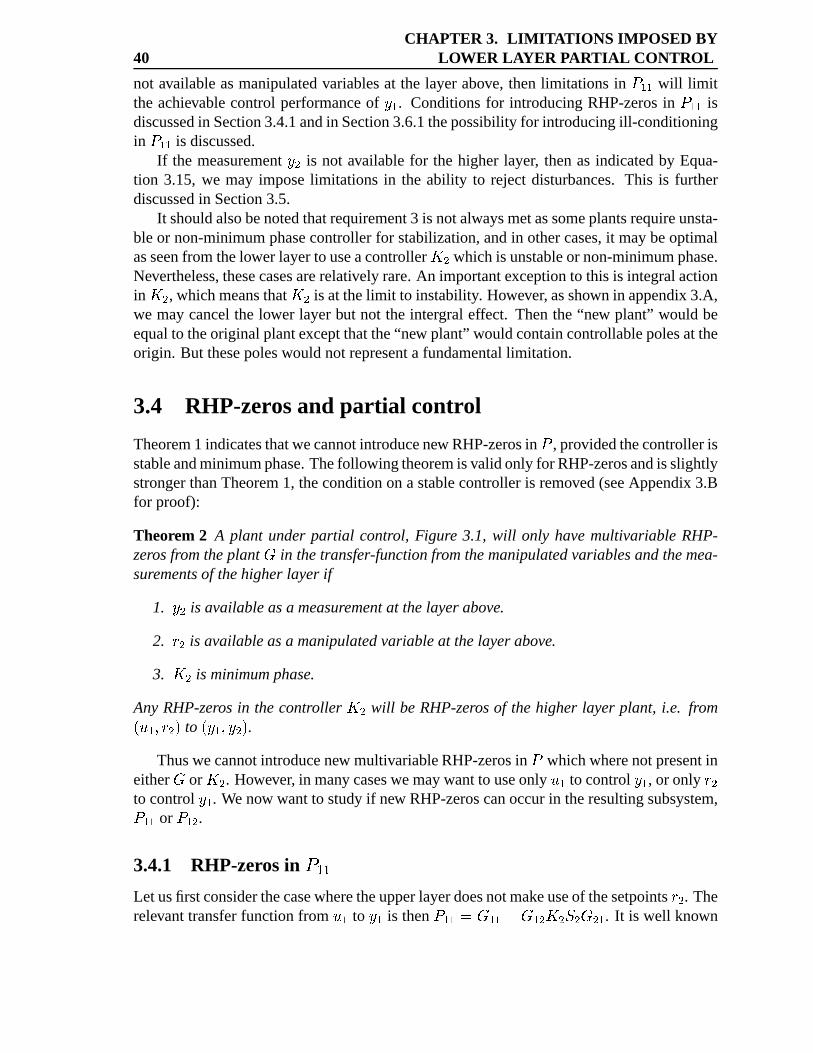
40CHAPTER 3. LIMIT ATIONS IMPOSED BY
LOWER LAYER PARTIAL CONTROL
not availableasmanipulatedvariablesat the layer above, thenlimitations in�����
will limitthe achievablecontrol performanceof # � . Conditionsfor introducingRHP-zerosin
�w���is
discussedin Section3.4.1andin Section3.6.1thepossibilityfor introducingill-conditioningin�����
is discussed.If the measurement# � is not availablefor the higher layer, thenasindicatedby Equa-
tion 3.15, we may imposelimitations in the ability to rejectdisturbances.This is furtherdiscussedin Section3.5.
It shouldalsobenotedthatrequirement3 is notalwaysmetassomeplantsrequireunsta-ble or non-minimumphasecontrollerfor stabilization,andin othercases,it maybeoptimalasseenfrom thelower layerto useacontroller � � whichis unstableor non-minimumphase.Nevertheless,thesecasesarerelatively rare.An importantexceptionto this is integralactionin � � , whichmeansthat � � is at thelimit to instability. However, asshown in appendix3.A,we maycancelthe lower layerbut not the intergral effect. Thenthe “new plant” would beequalto theoriginalplantexceptthatthe“new plant” wouldcontaincontrollablepolesat theorigin. But thesepoleswouldnot representa fundamentallimitation.
3.4 RHP-zerosand partial control
Theorem1 indicatesthatwecannotintroducenew RHP-zerosin�
, providedthecontrollerisstableandminimumphase.Thefollowing theoremis validonly for RHP-zerosandis slightlystrongerthanTheorem1, theconditionon a stablecontrolleris removed(seeAppendix3.Bfor proof):
Theorem 2 A plant underpartial control, Figure 3.1, will only havemultivariableRHP-zerosfromtheplant in thetransfer-functionfromthemanipulatedvariablesandthemea-surementsof thehigherlayer if
1. # � is availableasa measurementat thelayerabove.
2. ' � is availableasa manipulatedvariableat thelayerabove.
3. � � is minimumphase.
Any RHP-zeros in the controller � � will be RHP-zerosof the higher layer plant, i.e. from) $ � +Z' � . to ) # � +Z# � . .Thuswecannotintroducenew multivariableRHP-zerosin
�whichwherenotpresentin
either or � � . However, in many caseswemaywantto useonly $ � to control # � , or only ' �to control # � . Wenow wantto studyif new RHP-zeroscanoccurin theresultingsubsystem,�w���
or�w���
.
3.4.1 RHP-zerosin ÈCÉ�ÉLet usfirst considerthecasewheretheupperlayerdoesnotmakeuseof thesetpoints' � . Therelevanttransferfunctionfrom $ � to # � is then
�w��� % ��� 0 ��� � �§°±� �A� . It is well known
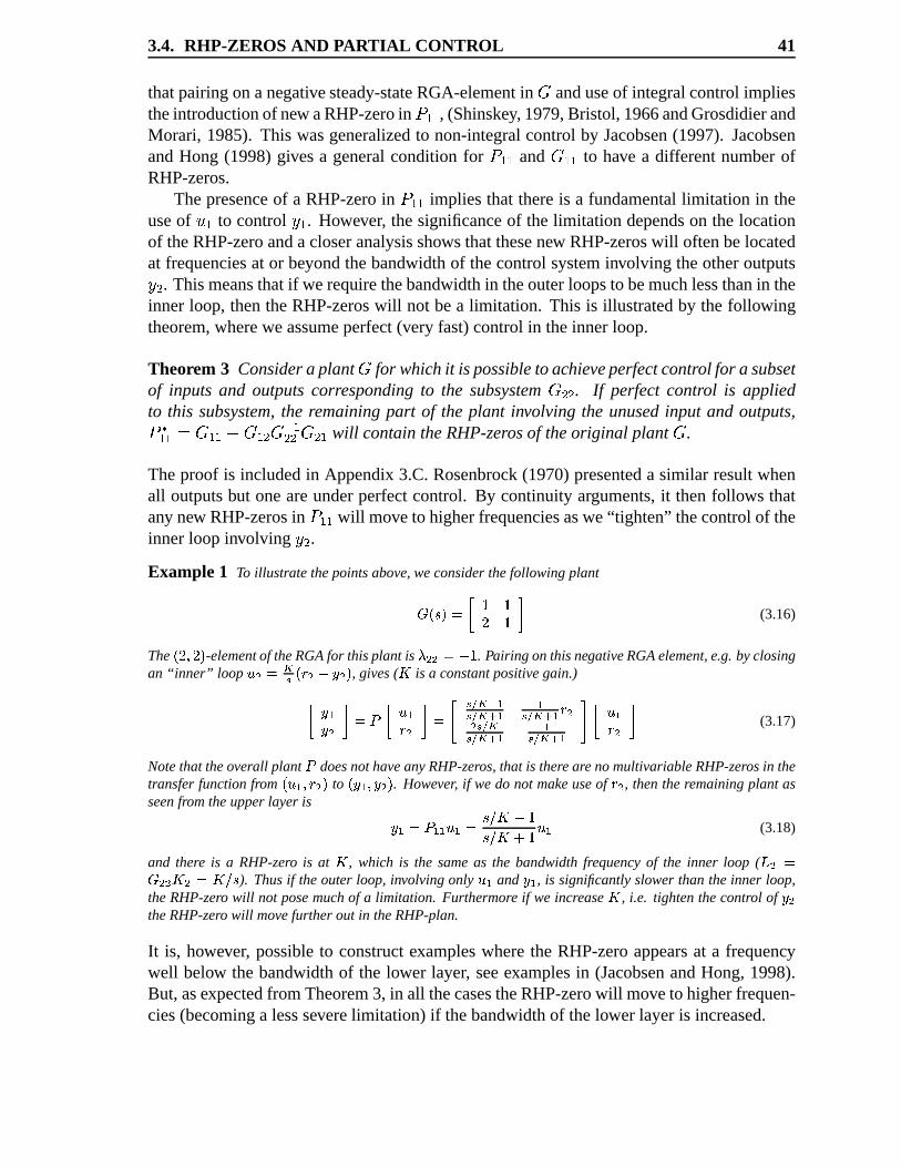
3.4. RHP-ZEROS AND PARTIAL CONTROL 41
thatpairingonanegativesteady-stateRGA-elementin anduseof integralcontrolimpliestheintroductionof new aRHP-zeroin
�w���, (Shinskey, 1979,Bristol,1966andGrosdidierand
Morari, 1985). This wasgeneralizedto non-integral controlby Jacobsen(1997). JacobsenandHong (1998)givesa generalconditionfor
�w���and ��� to have a differentnumberof
RHP-zeros.Thepresenceof a RHP-zeroin
�w���implies that thereis a fundamentallimitation in the
useof $ � to control # � . However, thesignificanceof the limitation dependson the locationof theRHP-zeroandacloseranalysisshowsthatthesenew RHP-zeroswill oftenbelocatedat frequenciesat or beyondthebandwidthof thecontrolsysteminvolving theotheroutputs# � . Thismeansthatif werequirethebandwidthin theouterloopsto bemuchlessthanin theinner loop, thentheRHP-zeroswill not bea limitation. This is illustratedby the followingtheorem,whereweassumeperfect(very fast)controlin theinnerloop.
Theorem 3 Consideraplant for which it is possibleto achieveperfectcontrol for a subsetof inputs and outputscorrespondingto the subsystem ��� . If perfectcontrol is appliedto this subsystem,the remainingpart of the plant involving the unusedinput and outputs,� ½��� % ��� 0 ��� PO ���� �A� will containtheRHP-zerosof theoriginal plant .
Theproof is includedin Appendix3.C.Rosenbrock(1970)presenteda similar resultwhenall outputsbut oneareunderperfectcontrol. By continuityarguments,it thenfollows thatany new RHP-zerosin
�����will moveto higherfrequenciesaswe“tighten” thecontrolof the
innerloop involving # � .Example 1 To illustratethepointsabove, weconsiderthefollowing plant]eʶcZËÍÌÏÎ ÉÐÉÑ ÉQÒ (3.16)
The Ê Ñ�ÓLÑ Ë -elementof theRGAfor thisplant is Ô bLb ÌÖÕ É . Pairing onthisnegativeRGAelement,e.g. byclosingan “inner” loop × b ÌÙØ Ú�ÊÜÛ b Õ¤Ý b Ë , gives( Þ is a constantpositivegain.)
Î Ý `Ý b Ò Ì�ßSÎ × `Û b Ò Ì ¡ Ú�à Ø ^�`Ú�à Ø�á ` `Ú�à Ø�á ` Û bb Ú�à ØÚ�à Ø�á ` `Ú�à Ø�á ` £ Î × `Û b Ò (3.17)
Notethat theoverall plant ß doesnothaveanyRHP-zeros,that is therearenomultivariableRHP-zerosin thetransferfunctionfrom Êâ× ` Ó Û b Ë to ÊÜÝ ` Ó Ý b Ë . However, if wedo not make useof Û b , thentheremainingplant asseenfromtheupperlayer is Ý ` Ì�ß `L` × ` Ì cZã§ÞäÕ ÉcZã§Þ»å É × ` (3.18)
and there is a RHP-zero is at Þ , which is the sameas the bandwidthfrequencyof the inner loop ( æ b Ì] bLb Þ b ÌçÞ�ã§c ). Thusif theouter loop, involvingonly × ` and Ý ` , is significantlyslowerthan theinner loop,theRHP-zero will not posemuch of a limitation. Furthermore if we increaseÞ , i.e. tightenthecontrol of Ý btheRHP-zero will movefurtherout in theRHP-plan.
It is, however, possibleto constructexampleswherethe RHP-zeroappearsat a frequencywell below the bandwidthof the lower layer, seeexamplesin (JacobsenandHong,1998).But, asexpectedfrom Theorem3, in all thecasestheRHP-zerowill moveto higherfrequen-cies(becominga lessseverelimitation) if thebandwidthof thelower layeris increased.
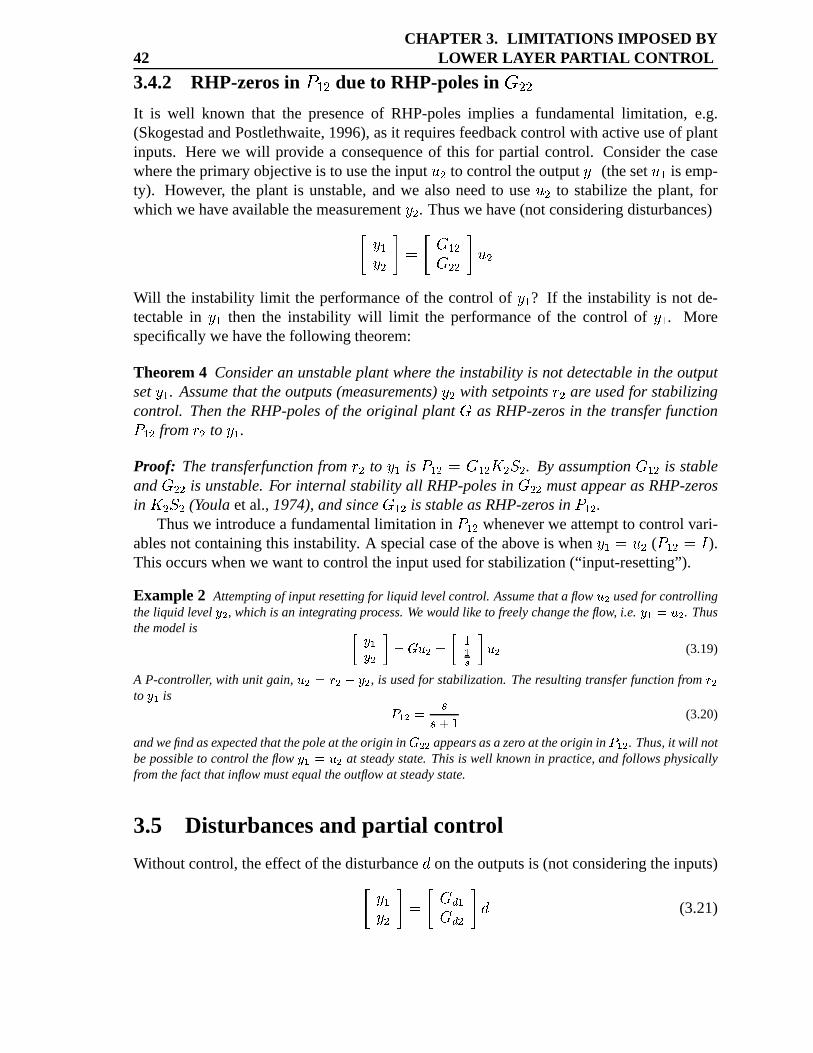
42CHAPTER 3. LIMIT ATIONS IMPOSED BY
LOWER LAYER PARTIAL CONTROL
3.4.2 RHP-zerosin ÈCÉ Ñ due to RHP-polesin è Ñ�ÑIt is well known that the presenceof RHP-polesimplies a fundamentallimitation, e.g.(SkogestadandPostlethwaite,1996),asit requiresfeedbackcontrolwith activeuseof plantinputs. Herewe will provide a consequenceof this for partial control. Considerthe casewheretheprimaryobjective is to usetheinput $ � to controltheoutput # � (theset $ � is emp-ty). However, the plant is unstable,andwe alsoneedto use $ � to stabilizethe plant, forwhich wehaveavailablethemeasurement# � . Thuswehave (notconsideringdisturbances)¡ # �# � £ % ¡ ��� ��� £ $ �Will the instability limit the performanceof the control of # � ? If the instability is not de-tectablein # � then the instability will limit the performanceof the control of # � . Morespecificallywehave thefollowing theorem:
Theorem 4 Consideran unstableplant where theinstability is not detectablein theoutputset # � . Assumethat theoutputs(measurements)# � with setpoints' � are usedfor stabilizingcontrol. ThentheRHP-polesof theoriginal plant asRHP-zeros in the transferfunction�w���
from ' � to # � .Proof: Thetransferfunctionfrom ' � to # � is
�w��� % ��� � ��°±� . By assumption ��� is stableand ��� is unstable. For internal stability all RHP-polesin ��� mustappearasRHP-zerosin � �§°±� (Youla et al., 1974),andsince ��� is stableasRHP-zerosin
�w���.
Thuswe introducea fundamentallimitation in�w���
wheneverwe attemptto controlvari-ablesnot containingthis instability. A specialcaseof theabove is when # � % $ � (
�w��� %Ϩ ).Thisoccurswhenwewantto controltheinputusedfor stabilization(“input-resetting”).
Example 2 Attemptingof input resettingfor liquid levelcontrol. Assumethata flow × b usedfor controllingtheliquid level Ý b , which is an integratingprocess.We wouldlike to freelychangetheflow, i.e. Ý ` Ì&× b . Thusthemodelis Î Ý `Ý b Ò Ì&]¼× b Ì Î É `Ú Ò × b (3.19)
A P-controller, with unit gain, × b ÌéÛ b Õ¾Ý b , is usedfor stabilization.Theresultingtransferfunctionfrom Û bto Ý ` is ß ` b Ì cc±å É (3.20)
andwefindasexpectedthat thepoleat theorigin in ] b7b appearsasa zero at theorigin in ß ` b . Thus,it will notbepossibleto control theflow Ý ` ÌÖ× b at steadystate. This is well knownin practice, andfollowsphysicallyfromthefact that inflow mustequaltheoutflowat steadystate.
3.5 Disturbancesand partial control
Withoutcontrol,theeffectof thedisturbance! on theoutputsis (notconsideringtheinputs)¡ # �# � £ % ¡ QB �QB � £ ! (3.21)
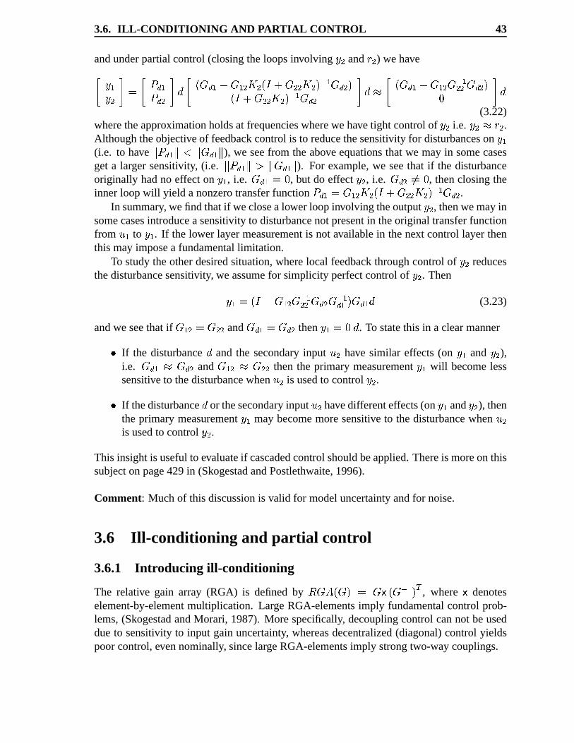
3.6. ILL-CONDITIONING AND PARTIAL CONTROL 43
andunderpartialcontrol(closingtheloopsinvolving # � and ' � ) wehave
¡ # �# � £ % ¡ � B �� B � £ ! ¡ ) QB � 0 ��� � � )�¨ J ��� � � . O � QB � .)�¨ J ��� � � . O � QB � £ ! ¿ ¡ ) CB � 0 ��� O ���� QB � .o £ !(3.22)
wheretheapproximationholdsat frequencieswherewehavetight controlof # � i.e. # �À¿ ' � .Althoughtheobjectiveof feedbackcontrolis to reducethesensitivity for disturbanceson # �(i.e. to have ê � B � ê¾ëqê�CB � ê ), we seefrom theabove equationsthatwe may in somecasesget a larger sensitivity, (i.e. ê � B � êjì¢ê�CB � ê ). For example,we seethat if the disturbanceoriginally hadno effect on # � , i.e. QB � % o
, but do effect # � , i.e. CB �îí% o, thenclosingthe
innerloopwill yield anonzerotransferfunction� B � % ��� � � )�¨ J ��� � � . O � QB � .
In summary, wefind thatif weclosealowerloopinvolving theoutput # � , thenwemayinsomecasesintroduceasensitivity to disturbancenotpresentin theoriginal transferfunctionfrom $ � to # � . If thelower layermeasurementis not availablein thenext control layerthenthis mayimposea fundamentallimitation.
To studytheotherdesiredsituation,wherelocal feedbackthroughcontrolof # � reducesthedisturbancesensitivity, weassumefor simplicity perfectcontrolof # � . Then# � %ï)�¨¤0 ��� O ���� CB � O �B � .;QB � ! (3.23)
andweseethatif ��� % ��� and QB � % CB � then # � % o ! . To statethis in aclearmanner If the disturbance! andthe secondaryinput $ � have similar effects (on # � and # � ),i.e. QB �P¿ CB � and ���ð¿ ��� thenthe primary measurement# � will becomelesssensitive to thedisturbancewhen $ � is usedto control # � . If thedisturbance! or thesecondaryinput $ � havedifferenteffects(on # � and # � ), thentheprimary measurement# � maybecomemoresensitive to thedisturbancewhen $ �is usedto control # � .
This insightis usefulto evaluateif cascadedcontrolshouldbeapplied.Thereis moreonthissubjecton page429in (SkogestadandPostlethwaite,1996).
Comment: Much of thisdiscussionis valid for modeluncertaintyandfor noise.
3.6 Ill-conditioning and partial control
3.6.1 Intr oducing ill-conditioning
The relative gain array (RGA) is definedby ñòQ� ) y. % 1� ) O � .�ó , where � denoteselement-by-elementmultiplication. LargeRGA-elementsimply fundamentalcontrolprob-lems,(SkogestadandMorari, 1987). More specifically, decouplingcontrolcannot beuseddueto sensitivity to input gainuncertainty, whereasdecentralized(diagonal)control yieldspoorcontrol,evennominally, sincelargeRGA-elementsimply strongtwo-waycouplings.
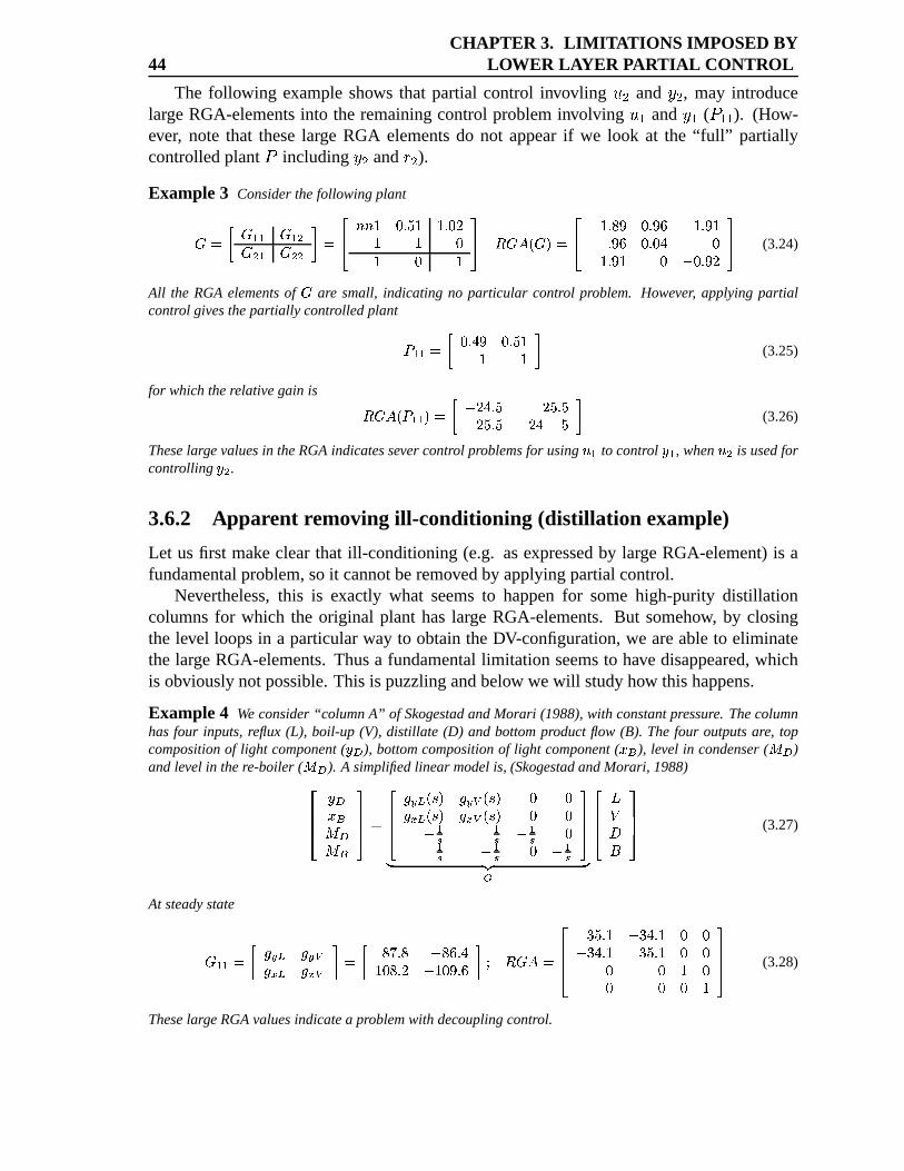
44CHAPTER 3. LIMIT ATIONS IMPOSED BY
LOWER LAYER PARTIAL CONTROL
The following exampleshows that partial control invovling $ � and # � , may introducelarge RGA-elementsinto the remainingcontrol probleminvolving $ � and # � (
�w���). (How-
ever, note that theselarge RGA elementsdo not appearif we look at the “full” partiallycontrolledplant
�including # � and ' � ).
Example 3 Considerthefollowingplant
]ÖÌ Î ] `L` ] ` b] b ` ] b7b Ò Ìõôök÷a÷ É¢ø�ù ú�É É�ù ø ÑÉ É øÉ ø ÉCûü ý ]�þ=ÊÜ]wË9Ìgôö Õ É�ù ÿ�� ø�ù ��� É�ù ��Éù ���Ðø�ù ø�� øÉ�ù ��É ø Õ ø�ù � Ñ ûü (3.24)
All the RGAelementsof ] are small, indicating no particular control problem. However, applyingpartialcontrol givesthepartially controlled plant ß `7` Ì Î ø�ù ���Ðø�ù ú�ÉÉ ÉyÒ (3.25)
for which therelativegain is ý ]�þ=ÊÜß `L` Ë Ì Î Õ Ñ �*ù ú Ñ ú�ù úÑ ú�ù ú Õ Ñ � Õ ú¾Ò (3.26)
Theselargevaluesin theRGAindicatessever control problemsfor using × ` to control Ý ` , when× b is usedforcontrolling Ý b .3.6.2 Apparent removing ill-conditioning (distillation example)
Let us first make clearthat ill-conditioning (e.g. asexpressedby large RGA-element)is afundamentalproblem,soit cannotberemovedby applyingpartialcontrol.
Nevertheless,this is exactly what seemsto happenfor somehigh-purity distillationcolumnsfor which the original plant haslarge RGA-elements.But somehow, by closingthe level loopsin a particularway to obtaintheDV-configuration,we areableto eliminatethe largeRGA-elements.Thusa fundamentallimitation seemsto have disappeared,whichis obviouslynotpossible.This is puzzlingandbelow wewill studyhow this happens.
Example 4 We consider“column A” of SkogestadandMorari (1988),with constantpressure. Thecolumnhasfour inputs,reflux(L), boil-up (V), distillate (D) and bottomproductflow (B). Thefour outputsare, topcompositionof light component( Ý�� ), bottomcompositionof light component( �� ), level in condenser( �� )andlevel in there-boiler( �� ). A simplifiedlinear modelis, (SkogestadandMorari, 1988)
ô��ö Ý �� ����� û ü Ì ô��ö ����� ʺcAË ����� ʺcZË ø ø��� � ʺcAË ��� � ʺcZË ø øÕ `Ú ` Ú Õ `Ú ø`Ú Õ `Ú ø Õ `Ú û üª «�¬ �
ô��ö æ�� � û ü (3.27)
At steadystate
] `L` Ì Î � ��� � ������ � ��� � Ò Ì Î ÿ���ù ÿ Õ ÿ���ù �ÉNø�ÿ�ù Ñ Õ ÉNø���ù � Ò�� ý ]�þ&Ì ô��ö� ú�ù�É Õ � ��ù�É ø øÕ � ��ù�É � ú�ù�É¢ø øø ø É©øø ø ø É û ü (3.28)
TheselargeRGAvaluesindicatea problemwith decouplingcontrol.
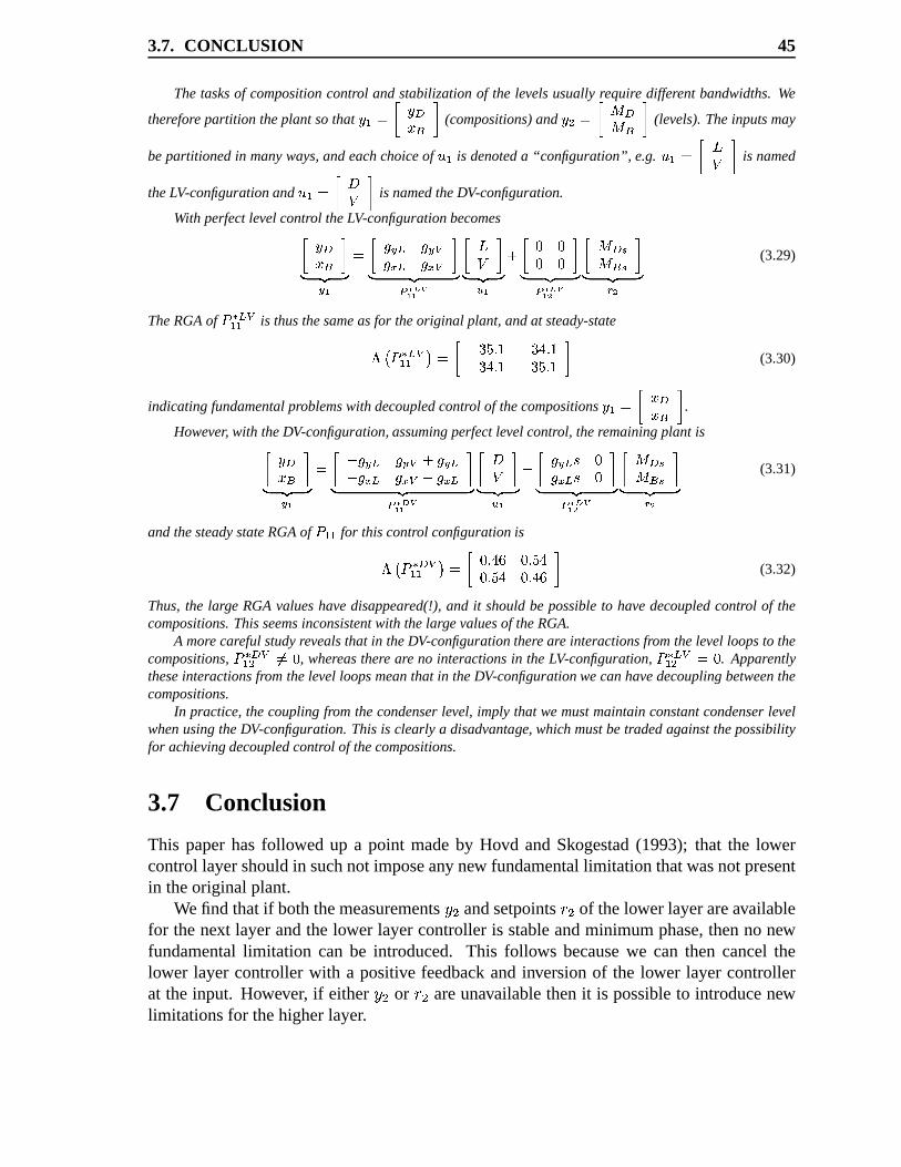
3.7. CONCLUSION 45
Thetasksof compositioncontrol andstabilizationof the levelsusuallyrequire different bandwidths.We
therefore partition theplant sothat Ý ` Ì Î Ý��� � Ò (compositions)and Ý b Ì Î �� � Ò (levels).Theinputsmay
bepartitionedin manyways,andeach choiceof × ` is denoteda “configuration”, e.g. × ` Ì Î æ� Ò is named
theLV-configurationand × ` Ì Î � � Ò is namedtheDV-configuration.
With perfectlevel control theLV-configurationbecomesÎ Ý �� � Òª «�¬ ���Ì Î ����� ������ � � � � � Òª «�¬ "!$#�%�&�
Î æ� Òª «�¬ ' �å Î ø øø ø Òª «�¬ "!(#�%�*)
Î � Ú � Ú Òª «V¬ + )(3.29)
TheRGAof ß-, ��`L` is thusthesameasfor theoriginal plant,andat steady-state
.0/ ß , ��`L` 1 Ì Î � ú�ù�É Õ � �*ù ÉÕ � ��ù�É � ú�ù�ÉCÒ (3.30)
indicatingfundamentalproblemswith decoupledcontrol of thecompositionsÝ ` ÌÏÎ ���� Ò .However, with theDV-configuration,assumingperfectlevel control, theremainingplant isÎ Ý���2� Òª «V¬ � �
Ì Î Õ � ��� � ��� å � ���Õ ��� � ��� � å ��� � Òª «�¬ "!(3%�4�Î � � Òª «�¬ ' �
å Î � ��� c ø��� � c ø Òª «�¬ "!(32%�*)Î �� Ú�� Ú Òª «�¬ + )
(3.31)
andthesteadystateRGAof ß `L` for thiscontrol configuration is
.5/ ß , � �`L` 1 Ì Î ø�ù ���Ðø�ù ú6�ø�ù ú6� ø�ù ���5Ò (3.32)
Thus,the large RGAvalueshavedisappeared(!), and it shouldbe possibleto havedecoupledcontrol of thecompositions.Thisseemsinconsistentwith thelargevaluesof theRGA.
A more careful studyrevealsthat in theDV-configurationthereare interactionsfromthelevel loopsto thecompositions,ß-, � �` b 7Ì ø , whereasthere are no interactionsin theLV-configuration, ß-, ��` b Ì ø . Apparentlytheseinteractionsfromthelevel loopsmeanthat in theDV-configurationwecanhavedecouplingbetweenthecompositions.
In practice, thecouplingfromthecondenserlevel, imply that wemustmaintainconstantcondenserlevelwhenusingtheDV-configuration. Thisis clearly a disadvantage, which mustbetradedagainstthepossibilityfor achievingdecoupledcontrol of thecompositions.
3.7 Conclusion
This paperhasfollowed up a point madeby Hovd andSkogestad(1993); that the lowercontrollayershouldin suchnot imposeany new fundamentallimitation thatwasnotpresentin theoriginal plant.
Wefind thatif boththemeasurements# � andsetpoints' � of thelower layerareavailablefor thenext layerandthe lower layercontrolleris stableandminimumphase,thenno newfundamentallimitation can be introduced. This follows becausewe can then cancelthelower layer controllerwith a positive feedbackandinversionof the lower layer controllerat the input. However, if either # � or ' � areunavailablethenit is possibleto introducenewlimitationsfor thehigherlayer.
46CHAPTER 3. LIMIT ATIONS IMPOSED BY
LOWER LAYER PARTIAL CONTROL
3.A Proof of Theorem1
We studythefollowing system(i.e. thepartially controlledsystemin Figure3.1,wheretheloop involving # � and $ � is closed)# � % ) ��� 0 ��� � �-°±� �A� .V$ ��J (3.33)) CB � 0 ��� � �§°±� CB � .N! J ��� � ��°±� ' �# � % °±� �A� $ �KJð±� QB � ! J°±� ��� � � ' �Here ' � is adegreeof freedomandweapplya ”two degreeof freedom”controller' � % �08Z$ Å v7Ç� 0 �09§# � (3.34)
Theresultingclosed-loopsystemis# � % )�¨ Jð±� ��� � � �09�. O � °±� ) �A� $ ��J QB � !/. J)�¨ Jð±� ��� � � �09�. O � °±� ��� � � �58Z$ Å v7Ç�If )�¨ J °±� ��� � � �:9�. O � °±� % ¨ thentheeffect of $ � and ! will becomethatof the originalplant. This is achieved if )�¨ J °±� ��� � �ª «V¬ ó�; �09�. % °±�
, which is satisfiedif �09 % 0 ¨ (i.e.
positive feedbackof unity gain).Then# � % ��� $ ��J QB � ! J ��� � � �08Z$ Šv7� (3.35)# � % �A� $ ��J QB � ! J ��� � � �08Z$ Šv7�To also restorethe original transferfunction from $ � to # , we need �08 % � O �� . Thus,� � hasto beminimumphaseandstable(otherwise� � � O �� would containhiddenunstablemodes).Thusminimumphasebehavior andinstabilitiesintroducedby thecontrollercannotbecanceledby thehigherlayer.
If thecontroller � � usesintegral actionthenby letting �58 beequal <� O �� , where � � %<� � 8 I and <� � is thestable,Equation3.35becomes# � % ��� $ �KJ CB � ! J ���I $ Šv�� (3.36)# � % �A� $ �KJ CB � ! J ���I $ Šv��
Providedthateither ��� or ��� doesnot have a RHP-zeroat theorigin thenthepoleat theorigin will becontrollablefrom $ Šv�� . Thustheonly differencebetweentheaboveplantandtheoriginal plant is that it containsa poleat theorigin which is not really a fundamentallimitation.
Comment: It is well-known thatzerosof aplantarenotmovedby feedbackcontrol,i.e.thezerosof Q� and )�¨ J y�ç. O � y� arethesame.However, asnotedfrom Equation3.9,partialcontrolis notaspecialcaseof feedbackcontrol,andthis is why wehave(re-)derivedTheorem2.
3.7. CONCLUSION 47
3.B Proof of Theorem2
For thesakeof argumentwe let �08 in Equation3.35beequalto ¨ , then
# % ¡ ¨ oo � � £ $ Å v7Ç� J QB�! (3.37)
Fromtheabove equationwe canclearlyseethatany RHP-zerosof thepartially controlledplanthasto comefrom either or � � evenif � � hasRHP-poles.
3.C Proof of Theorem3
Thepartially controlledplantis ����� % ��� 0 ��� O ���� �A� (3.38)
Thedeterminantof thepartially controlledplantis²>=�? ����� % ²@=�? ) ��� 0 ��� O ���� �A� . (3.39)
UsingSchursformulagives(andassumingthat ²>=�?Í ���¤í% o )²>=�? �w��� % ²@=�?Ͳ>=�?Í ��� (3.40)
The determinantof a systemcan be written in terms of the zero and pole polynomial,(MacFarlaneandKarcanias,1976):
²@=�?Í % � �Æ)LI .AU)LI . (3.41)
²@=�?Í ��� % � ��� � ��� )LI .A ��� )7I . (3.42)
where � and A arezeroandpolepolynomial(maynot necessarilyberelatively prime)andcis aconstant.Thus ²>=�? ����� %h� 8 � ��� �� ��� A ���A (3.43)
Sincethe rootsof A ��� hasto be rootsin A , they will not contribute to any zerosin ²@=�? �w��� .Secondlysinceweassumethat ��� is usedfor perfectcontrolit cannothaveany RHP-zeros.Which meansthatany RHP-zerosin ²>=�? ����� will have to comefrom � , e.g.from .

Chapter 4
Control of Reactor, SeparatorandRecyclePart I: Liquid phasesystems
T. Larsson,S.SkogestadandC. C. Yu
Partsof this work wherepresentedat NPCW-1998Stockholm,CAPEForum99 Li egeandAIChE annualmeeting1999,Dallas.
We considerthecontrolstructureselectionfor a simpleplantwith a liquid phasereactor, a distillation column
andrecycle of unreactedreactants.This classof plantshasbeenstudiedextensively in the literature.Luyben
hasusedit asa basisfor his genericrule, “fix a flow in a liquid recycle loop”. In this paperwe shows that the
basisfor his rule is questionable.This is basedon a systematicselectionof thecontrolstructure,by usingthe
conceptof self-optimizingcontrol.
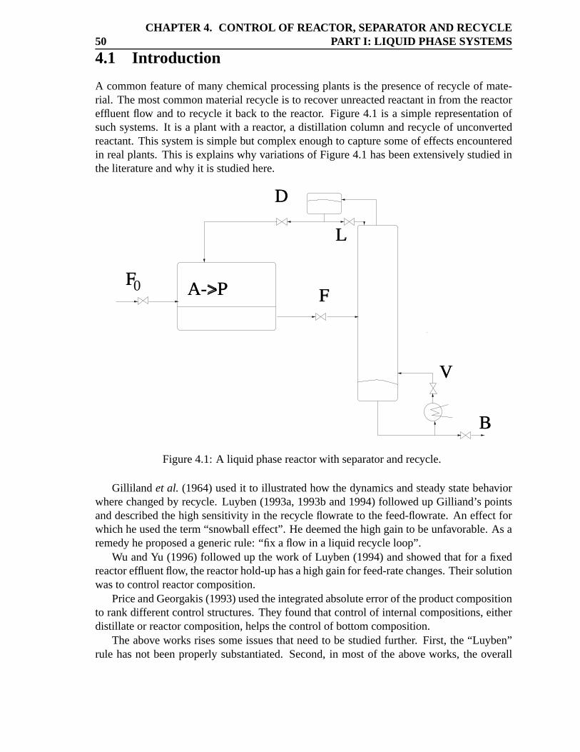
50CHAPTER 4. CONTROL OF REACTOR, SEPARATOR AND RECYCLE
PART I: LIQ UID PHASE SYSTEMS
4.1 Intr oduction
A commonfeatureof many chemicalprocessingplantsis thepresenceof recycle of mate-rial. Themostcommonmaterialrecycle is to recover unreactedreactantin from thereactoreffluent flow andto recycle it backto the reactor. Figure4.1 is a simplerepresentationofsuchsystems.It is a plant with a reactor, a distillation columnandrecycle of unconvertedreactant.This systemis simplebut complex enoughto capturesomeof effectsencounteredin realplants.This is explainswhy variationsof Figure4.1 hasbeenextensively studiedintheliteratureandwhy it is studiedhere.
0F A->P F
D
V
B
L
Figure4.1: A liquid phasereactorwith separatorandrecycle.
Gilliland et al. (1964)usedit to illustratedhow thedynamicsandsteadystatebehaviorwherechangedby recycle. Luyben(1993a,1993band1994)followedup Gilliand’s pointsanddescribedthehigh sensitivity in therecycle flowrateto thefeed-flowrate. An effect forwhich heusedtheterm“snowball effect”. He deemedthehigh gainto beunfavorable.As aremedyheproposedagenericrule: “fix aflow in a liquid recycle loop”.
Wu andYu (1996)followedup thework of Luyben(1994)andshowedthat for a fixedreactoreffluentflow, thereactorhold-uphasahighgainfor feed-ratechanges.Theirsolutionwasto controlreactorcomposition.
PriceandGeorgakis(1993)usedtheintegratedabsoluteerrorof theproductcompositionto rankdifferentcontrolstructures.They foundthatcontrolof internalcompositions,eitherdistillateor reactorcomposition,helpsthecontrolof bottomcomposition.
Theabove works risessomeissuesthatneedto be studiedfurther. First, the “Luyben”rule hasnot beenproperlysubstantiated.Second,in mostof the above works, the overall
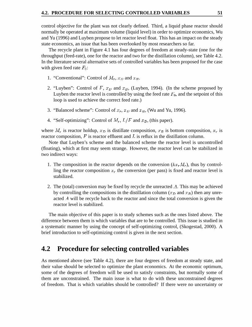
4.2. PROCEDURE FOR SELECTING CONTROLLED VARIABLES 51
controlobjective for theplantwasnot clearlydefined.Third, a liquid phasereactorshouldnormallybeoperatedatmaximumvolume(liquid level) in orderto optimizeeconomics,WuandYu (1996)andLuybenproposeto let reactorlevel float. Thishasanimpactonthesteadystateeconomics,anissuethathasbeenoverlookedby mostresearcherssofar.
Therecycle plant in Figure4.1 hasfour degreesof freedomat steady-state(onefor thethroughput(feed-rate),onefor thereactorandtwo for thedistillationcolumn),seeTable4.2.In theliteratureseveralalternativesetsof controlledvariableshasbeenproposedfor thecasewith givenfeedrate BDC :
1. “Conventional”: Controlof EGF , HJI and HJK .
2. “Luyben”: Control of B , HJI and HJK , (Luyben,1994). (In the schemeproposedbyLuybenthereactorlevel is controlledby usingthefeedrate BLC , andthesetpointof thisloop is usedto achieve thecorrectfeedrate.)
3. “Balancedscheme”:Controlof HMF , HJI and HJK , (Wu andYu, 1996).
4. “Self-optimizing”: Controlof EGF , NPOB and HJK , (thispaper).
where EGF is reactorholdup, HJI is distillate composition,HJK is bottomcomposition,HMF isreactorcomposition,B is reactoreffluentand N is reflux in thedistillationcolumn.
Note that Luyben’s schemeand the balancedschemethe reactorlevel is uncontrolled(floating),which at first mayseemstrange.However, the reactorlevel canbe stabilizedintwo indirectways:
1. Thecompositionin the reactordependson theconversion( QRHMF�EGF ), thusby control-ling the reactorcompositionHMF theconversion(perpass)is fixedandreactorlevel isstabilized.
2. The(total)conversionmaybefixedby recycle theunreactedS . Thismaybeachievedby controllingthecompositionsin thedistillation column( HJI and HJK ) thenany unre-actedS will berecycle backto thereactorandsincethetotal conversionis giventhereactorlevel is stabilized.
Themainobjective of this paperis to studyschemessuchastheoneslistedabove. Thedifferencebetweenthemis which variablesthatareto becontrolled.This issueis studiedina systematicmannerby usingtheconceptof self-optimizingcontrol, (Skogestad,2000). Abrief introductionto self-optimizingcontrolis givenin thenext section.
4.2 Procedure for selectingcontrolled variables
As mentionedabove (seeTable4.2), therearefour degreesof freedomat steadystate,andtheir valueshouldbeselectedto optimizetheplanteconomics.At theeconomicoptimum,someof the degreesof freedomwill be usedto satisfyconstraints,but normally someofthem are unconstrained.The main issueis what to do with theseunconstraineddegreesof freedom. That is which variablesshouldbe controlled?If therewereno uncertaintyor
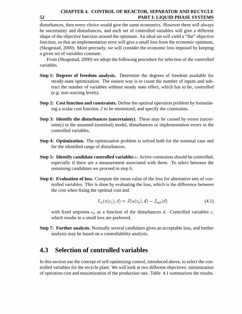
52CHAPTER 4. CONTROL OF REACTOR, SEPARATOR AND RECYCLE
PART I: LIQ UID PHASE SYSTEMS
disturbances,theneverychoicewouldgive thesameeconomics.However therewill alwaysbe uncertaintyanddisturbances,andeachsetof controlledvariableswill give a differentshapeof theobjectivefunctionaroundtheoptimum.An idealsetwill yield a “flat” objectivefunction,sothatanimplementationerrorwill giveasmalllossfrom theeconomicoptimum,(Skogestad,2000).More precisely, we will considertheeconomiclossimposedby keepingagivensetof variablesconstant.
From(Skogestad,2000)weadoptthefollowing procedurefor selectionof thecontrolledvariables.
Step1: Degreesof fr eedom analysis. Determinethe degreesof freedomavailable forsteady-stateoptimization.Theeasiestway is to countthenumberof inputsandsub-tract the numberof variableswithout steadystateeffect, which hasto be,controlled(e.g.nonreactinglevels).
Step2: Cost function and constraints. Definetheoptimaloperationproblemby formulat-ing ascalarcostfunction T to beminimized,andspecifytheconstraints.
Step3: Identify the disturbances(uncertainty). Thesemaybe causedby errors(uncer-tainty) in theassumed(nominal)model,disturbancesor implementationerrorsin thecontrolledvariables.
Step4: Optimization. Theoptimizationproblemis solvedboth for thenominalcaseandfor theidentifiedrangeof disturbances.
Step5: Identify candidatecontrolled variables U . Activeconstraintsshouldbecontrolled,especiallyif thereare a measurementassociatedwith them. To selectbetweentheremainingcandidatesweproceedto step6.
Step6: Evaluation of loss.Computethemeanvalueof thelossfor alternativesetsof con-trolled variables.This is doneby evaluatingtheloss,which is thedifferencebetweenthecostwhenfixing theoptimalcostand
N�V>W$XDWYU�Z�[�\6]R[_^`T_WaXDWYU�Z�[�\6]R[DbcTedgf�h6WY]R[ (4.1)
with fixed setpointsU�Z as a function of the disturbances] . Controlledvariables U ,which resultsin asmall lossarepreferred.
Step7: Further analysis.Normallyseveralcandidatesgivesanacceptableloss,andfurtheranalysismaybebasedon acontrollabilityanalysis.
4.3 Selectionof controlled variables
In thissectionusetheconceptof self-optimizingcontrol,introducedabove,to selectthecon-trolledvariablesfor therecycleplant.Wewill look at two differentobjectives:minimizationof operationcostandmaximizationof theproductionrate.Table 4.1summarizestheresults.
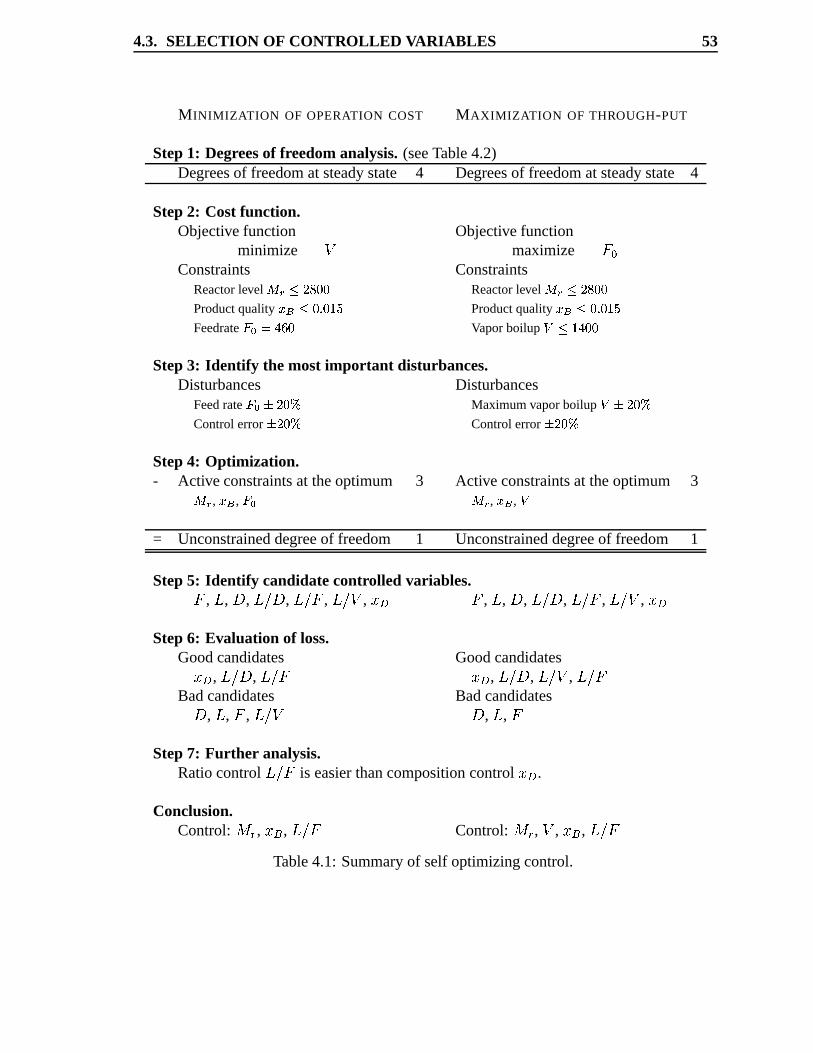
4.3. SELECTION OF CONTROLLED VARIABLES 53
M INIMIZATION OF OPERATION COST MAXIMIZATION OF THROUGH-PUT
Step1: Degreesof fr eedomanalysis.(seeTable4.2)Degreesof freedomat steadystate 4 Degreesof freedomat steadystate 4
Step2: Cost function.Objective function Objective function
minimize i maximize BLCConstraints Constraints
Reactorlevel j�kmlon�p�q�q Reactorlevel j�kmlon�p�q�qProductquality rstltqvu qvwyx Productquality rsolzqvu qvw�xFeedrate{"|m}t~���q Vaporboilup ��l�w�~�q�q
Step3: Identify the most important disturbances.Disturbances Disturbances
Feedrate {"|��5n�q�� Maximumvaporboilup ���5n�q��Controlerror ��n�q�� Controlerror ��n�q��
Step4: Optimization.- Activeconstraintsat theoptimum 3 Activeconstraintsat theoptimum 3j k , r s , { | j k , r s , �= Unconstraineddegreeof freedom 1 Unconstraineddegreeof freedom 1
Step5: Identify candidatecontrolled variables.B , N , � , N-O2� , N-O2B , N-Oei , HJI B , N , � , N-O2� , N-O2B , N-Oei , HJIStep6: Evaluation of loss.
Goodcandidates GoodcandidatesHJI , N-O2� , N-O2B HJI , NPO� , N-Oei , N-O2B
Badcandidates Badcandidates� , N , B , N-Oei � , N , B
Step7: Further analysis.Ratiocontrol NPOB is easierthancompositioncontrol HJI .
Conclusion.Control: EGF , HJK , N-O2B Control: EGF , i , HJK , N-O2B
Table4.1: Summaryof self optimizingcontrol.
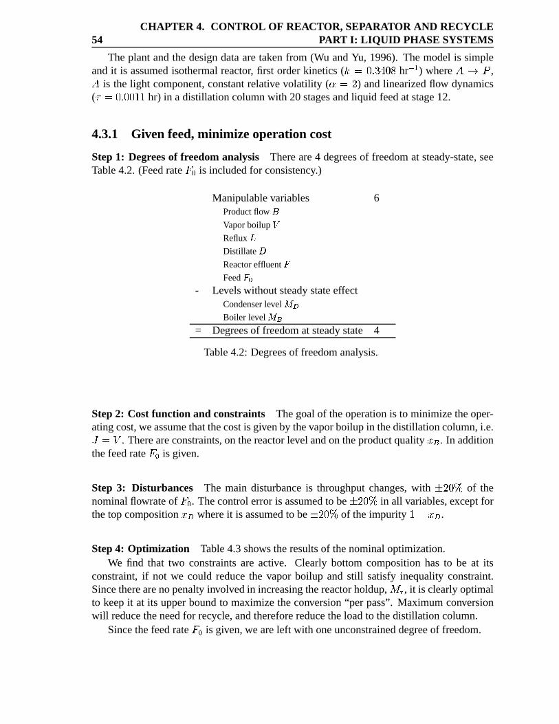
54CHAPTER 4. CONTROL OF REACTOR, SEPARATOR AND RECYCLE
PART I: LIQ UID PHASE SYSTEMS
Theplantandthedesigndataaretaken from (Wu andYu, 1996). Themodelis simpleandit is assumedisothermalreactor, first orderkinetics( Q�^��@���2���2� hr�M� ) where S�� � ,S is the light component,constantrelative volatility ( ��^�� ) andlinearizedflow dynamics( �t^��@���e�@�2� hr) in a distillationcolumnwith 20stagesandliquid feedat stage12.
4.3.1 Given feed,minimize operation cost
Step1: Degreesof fr eedomanalysis Thereare4 degreesof freedomat steady-state,seeTable4.2. (Feedrate BDC is includedfor consistency.)
Manipulablevariables 6Productflow �Vaporboilup �Reflux �Distillate �Reactoreffluent {Feed{"|
- LevelswithoutsteadystateeffectCondenserlevel j� Boiler level j s
= Degreesof freedomat steadystate 4
Table4.2: Degreesof freedomanalysis.
Step2: Cost function and constraints Thegoalof theoperationis to minimizetheoper-atingcost,weassumethatthecostis givenby thevaporboilup in thedistillationcolumn,i.e.T¡^¢i . Thereareconstraints,on thereactorlevel andontheproductquality HJK . In additionthefeedrate BLC is given.
Step 3: Disturbances The main disturbanceis throughputchanges,with £¤�2�e¥ of thenominalflowrateof BLC . Thecontrolerroris assumedto be £¦�2��¥ in all variables,exceptforthetopcompositionHJI whereit is assumedto be £¤���¥ of theimpurity �§b¨HJI .
Step4: Optimization Table4.3showstheresultsof thenominaloptimization.We find that two constraintsare active. Clearly bottom compositionhasto be at its
constraint,if not we could reducethe vaporboilup and still satisfy inequality constraint.Sincetherearenopenaltyinvolvedin increasingthereactorholdup, EGF , it is clearlyoptimalto keepit at its upperboundto maximizetheconversion“per pass”.Maximumconversionwill reducetheneedfor recycle,andthereforereducetheloadto thedistillationcolumn.
Sincethefeedrate BDC is given,weareleft with oneunconstraineddegreeof freedom.
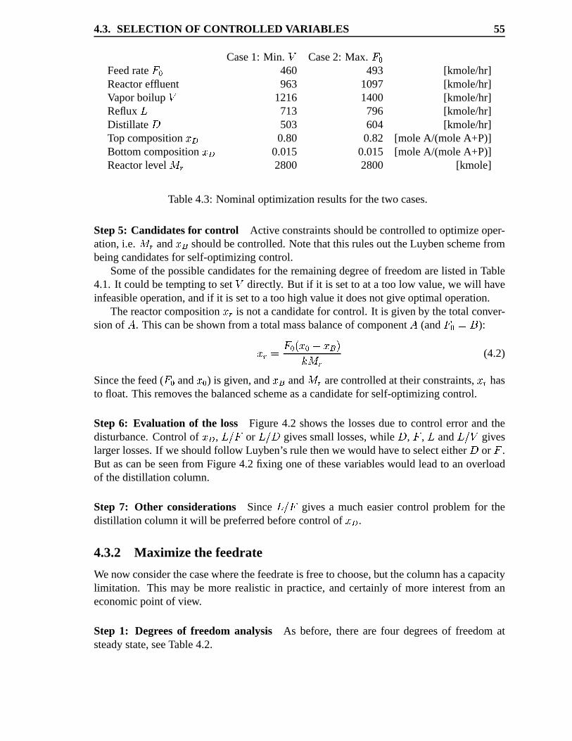
4.3. SELECTION OF CONTROLLED VARIABLES 55
Case1: Min. i Case2: Max. BDCFeedrate BDC 460 493 [kmole/hr]Reactoreffluent 963 1097 [kmole/hr]Vaporboilup i 1216 1400 [kmole/hr]Reflux N 713 796 [kmole/hr]Distillate � 503 604 [kmole/hr]Top compositionHJI 0.80 0.82 [mole A/(moleA+P)]BottomcompositionHJI 0.015 0.015 [mole A/(moleA+P)]Reactorlevel EGF 2800 2800 [kmole]
Table4.3: Nominaloptimizationresultsfor thetwo cases.
Step5: Candidatesfor control Activeconstraintsshouldbecontrolledto optimizeoper-ation,i.e. E©F and HJK shouldbecontrolled.Notethatthis rulesout theLuybenschemefrombeingcandidatesfor self-optimizingcontrol.
Someof thepossiblecandidatesfor theremainingdegreeof freedomarelistedin Table4.1. It couldbetemptingto set i directly. But if it is setto at a too low value,we will haveinfeasibleoperation,andif it is setto a toohighvalueit doesnotgiveoptimaloperation.
ThereactorcompositionHMF is not acandidatefor control. It is givenby thetotal conver-sionof S . Thiscanbeshown from a totalmassbalanceof componentS (and BLCª^�« ):
HMF¬^ BLCvW$HC-b¨HJKL[Q>EGF (4.2)
Sincethefeed( BDC and HC ) is given,and HJK and EGF arecontrolledat their constraints,HMF hasto float. This removesthebalancedschemeasacandidatefor self-optimizingcontrol.
Step 6: Evaluation of the loss Figure4.2 shows the lossesdueto control error andthedisturbance.Controlof HJI , N-O2B or N-O2� givessmall losses,while � , B , N and N-Oei giveslargerlosses.If weshouldfollow Luyben’s rule thenwewouldhave to selecteither � or B .But ascanbeseenfrom Figure4.2 fixing oneof thesevariableswould leadto anoverloadof thedistillationcolumn.
Step 7: Other considerations Since N-O2B givesa mucheasiercontrol problemfor thedistillationcolumnit will bepreferredbeforecontrolof HJI .
4.3.2 Maximize the feedrate
Wenow considerthecasewherethefeedrateis freeto choose,but thecolumnhasacapacitylimitation. This may be morerealistic in practice,andcertainlyof more interestfrom aneconomicpoint of view.
Step 1: Degreesof fr eedomanalysis As before, thereare four degreesof freedomatsteadystate,seeTable4.2.
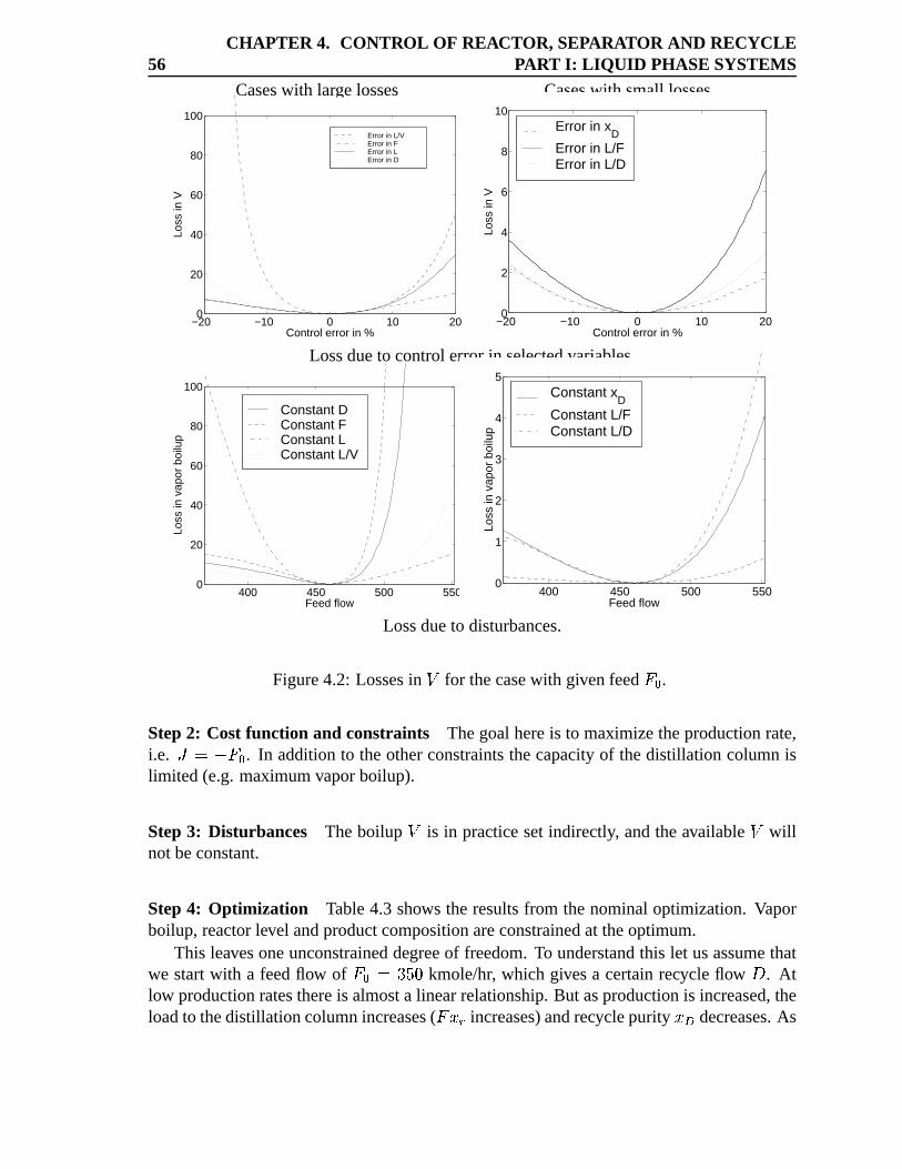
56CHAPTER 4. CONTROL OF REACTOR, SEPARATOR AND RECYCLE
PART I: LIQ UID PHASE SYSTEMS
Caseswith largelosses Caseswith small losses
−20 −10 0 10 200
20
40
60
80
100
Control error in %
Loss
in V
Error in L/VError in FError in LError in D
−20 −10 0 10 200
2
4
6
8
10
Control error in %
Loss
in V
Error in xD
Error in L/FError in L/D
Lossdueto controlerrorin selectedvariables.
400 450 500 5500
20
40
60
80
100
Feed flow
Loss
in v
apor
boi
lup
Constant DConstant FConstant LConstant L/V
400 450 500 5500
1
2
3
4
5
Feed flow
Loss
in v
apor
boi
lup
Constant xD
Constant L/FConstant L/D
Lossdueto disturbances.
Figure4.2: Lossesin i for thecasewith givenfeed BDC .
Step2: Cost function and constraints Thegoalhereis to maximizetheproductionrate,i.e. T®^¯b°BDC . In additionto theotherconstraintsthecapacityof thedistillation columnislimited (e.g.maximumvaporboilup).
Step3: Disturbances Theboilup i is in practicesetindirectly, andtheavailable i willnotbeconstant.
Step4: Optimization Table4.3 shows theresultsfrom thenominaloptimization.Vaporboilup, reactorlevel andproductcompositionareconstrainedat theoptimum.
This leavesoneunconstraineddegreeof freedom.To understandthis let usassumethatwe startwith a feedflow of BLC�^¯�e±2� kmole/hr, which givesa certainrecycle flow � . Atlow productionratesthereis almosta linearrelationship.But asproductionis increased,theloadto thedistillationcolumnincreases( B²HMF increases)andrecyclepurity HJI decreases.As
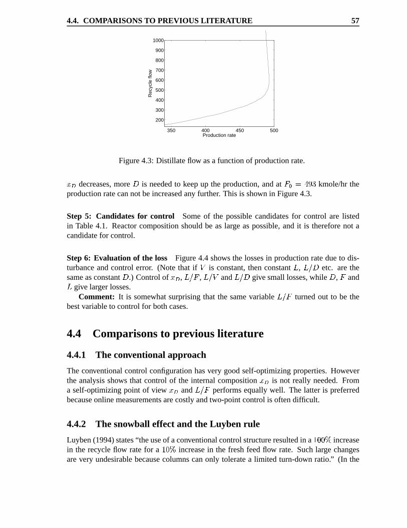
4.4. COMPARISONS TO PREVIOUS LITERA TURE 57
350 400 450 500
200
300
400
500
600
700
800
900
1000
Production rate
Rec
ycle
flow
Figure4.3: Distillate flow asa functionof productionrate.
HJI decreases,more � is neededto keepup theproduction,andat BDC³^´��µ2� kmole/hrtheproductionratecannotbeincreasedany further. This is shown in Figure4.3.
Step 5: Candidates for control Someof the possiblecandidatesfor control are listedin Table4.1. Reactorcompositionshouldbe aslarge aspossible,andit is thereforenot acandidatefor control.
Step6: Evaluation of the loss Figure4.4 shows the lossesin productionratedueto dis-turbanceandcontrol error. (Note that if i is constant,thenconstantN , NPO� etc. arethesameasconstant� .) Controlof HJI , N-O2B , N-Oei and NPO� givesmalllosses,while � , B andN give largerlosses.
Comment: It is somewhat surprisingthat the samevariable NPOB turnedout to be thebestvariableto controlfor bothcases.
4.4 Comparisonsto previous literatur e
4.4.1 The conventional approach
Theconventionalcontrol configurationhasvery goodself-optimizingproperties.Howeverthe analysisshows that control of the internalcompositionHJI is not really needed.Froma self-optimizingpoint of view HJI and N-O2B performsequallywell. The latter is preferredbecauseonlinemeasurementsarecostlyandtwo-pointcontrolis oftendifficult.
4.4.2 The snowball effectand the Luyben rule
Luyben(1994)states“the useof aconventionalcontrolstructureresultedin a �¶�e��¥ increasein the recycle flow ratefor a �¶��¥ increasein the freshfeedflow rate. Suchlarge changesarevery undesirablebecausecolumnscanonly toleratea limited turn-down ratio.” (In the
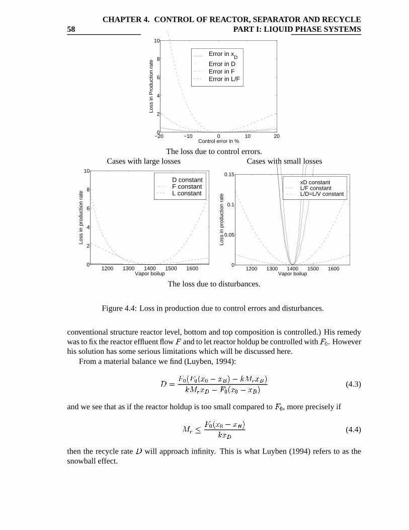
58CHAPTER 4. CONTROL OF REACTOR, SEPARATOR AND RECYCLE
PART I: LIQ UID PHASE SYSTEMS
−20 −10 0 10 200
2
4
6
8
10
Control error in %
Loss
in P
rodu
ctio
n ra
te
Error in xD
Error in DError in FError in L/F
Thelossdueto controlerrors.Caseswith largelosses Caseswith small losses
1200 1300 1400 1500 16000
2
4
6
8
10
Vapor boilup
Loss
in p
rodu
ctio
n ra
te
D constantF constantL constant
1200 1300 1400 1500 16000
0.05
0.1
0.15
Vapor boilup
Loss
in p
rodu
ctio
n ra
te
xD constantL/F constantL/D=L/V constant
Thelossdueto disturbances.
Figure4.4: Lossin productiondueto controlerrorsanddisturbances.
conventionalstructurereactorlevel, bottomandtop compositionis controlled.)His remedywasto fix thereactoreffluentflow B andto let reactorholdupbecontrolledwith BDC . Howeverhissolutionhassomeseriouslimitationswhichwill bediscussedhere.
Fromamaterialbalancewefind (Luyben,1994):
��^ BDC·WYBLC·W$HC¸b¨HJKL[mb¹Q>EGF�HJKD[Q>EGF�HJIGb®BLCvW$HC-b¨HJKL[ (4.3)
andweseethatasif thereactorholdupis too smallcomparedto BDC , morepreciselyif
EGF»º BLC·W$HC¸b¨HJKL[Q¼HJI (4.4)
thenthe recycle rate � will approachinfinity. This is whatLuyben(1994)refersto asthesnowball effect.
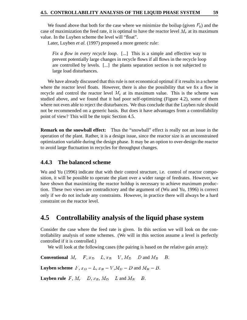
4.5. CONTROLLABILITY ANALYSIS OF THE LIQ UID PHASE SYSTEM 59
We foundabove thatbothfor thecasewherewe minimizetheboilup (given BLC ) andthecaseof maximizationthefeedrate,it is optimalto have thereactorlevel EGF at its maximumvalue.In theLuybenschemethelevel will “float”.
Later, Luybenet al. (1997)proposedamoregenericrule:
Fix a flow in every recycleloop. [...] This is a simple and effective way topreventpotentiallylargechangesin recycleflows if all flows in therecycle looparecontrolledby levels. [...] the plantsseparationsectionis not subjectedtolargeloaddisturbances.
Wehavealreadydiscussedthatthisruleis noteconomicaloptimalif it resultsin aschemewherethe reactorlevel floats. However, thereis also the possibility that we fix a flow inrecycle and control the reactorlevel EGF at its maximumvalue. This is the schemewasstudiedabove, andwe found that it hadpoor self-optimizing(Figure 4.2), someof themwherenotevenableto rejectthedisturbances.WethusconcludethattheLuybenruleshouldnot berecommendedon a genericbasis.But doesit have advantagesfrom a controllabilitypoint of view? Thiswill bethetopicSection4.5.
Remark on the snowball effect: Thusthe “snowball” effect is really not an issuein theoperationof theplant. Rather, it is a designissue,sincethereactorsizeis anunconstrainedoptimizationvariableduringthedesignphase.It maybeanoptionto over-designthereactorto avoid largefluctuationin recyclesfor throughputchanges.
4.4.3 The balancedscheme
Wu andYu (1996)indicatethatwith their control structure,i.e. control of reactorcompo-sition, it will bepossibleto operatetheplantover a wider rangeof feedrates.However, wehave shown thatmaximizingthe reactorholdupis necessaryto achieve maximumproduc-tion. Thesetwo views arecontradictoryandtheargumentof (Wu andYu, 1996)is correctonly if we do not includeany constraints.However, in practicetherewill alwaysbea hardconstrainton thereactorlevel.
4.5 Controllability analysisof the liquid phasesystem
Considerthe casewherethe feed rate is given. In this sectionwe will look on the con-trollability analysisof someschemes.(We will in this sectionassumea level is perfectlycontrolledif it is controlled.)
Wewill look at thefollowing cases(thepairingis basedon therelativegainarray):
Conventional EGF-b½B , HJI�b®N , HJK�b¹i , E�I©b®� and E�K¾b®« .
Luyben scheme B , HJI�b®N , HJK¡b®i , E�I�b®� and E�K�b®« .
Luyben rule B , EGF¸b®� , HJK , E¿IGb½N and E¿K¡b½« .
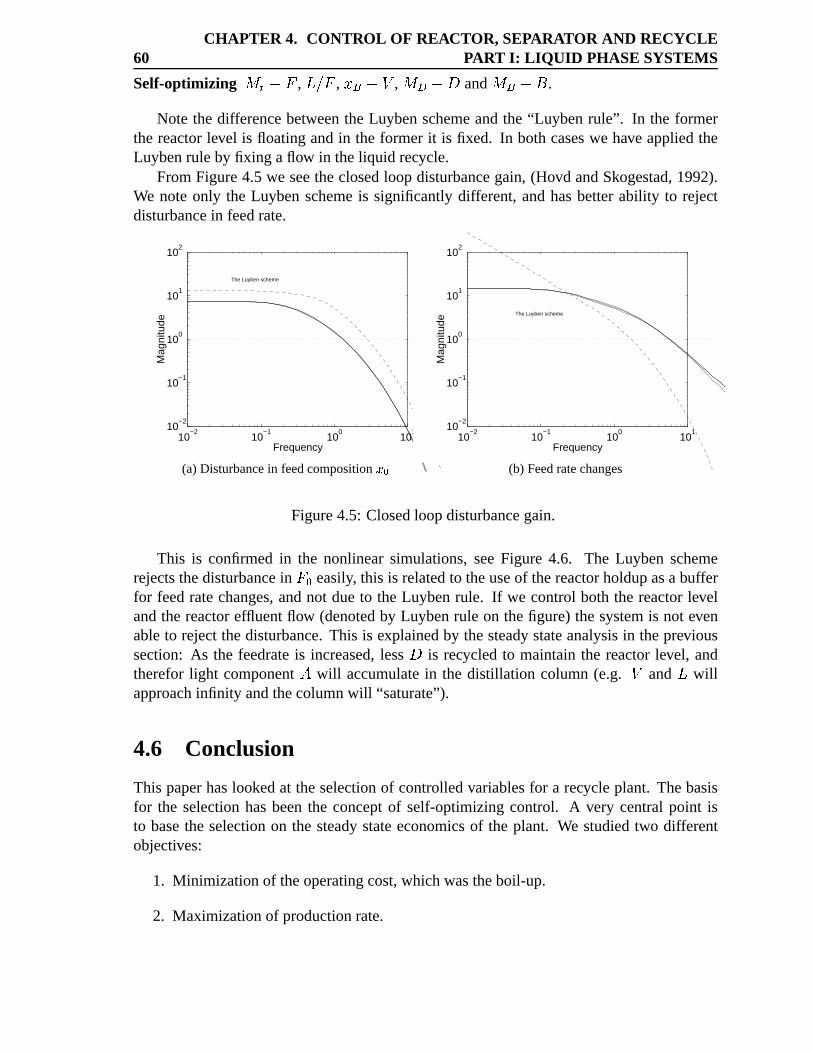
60CHAPTER 4. CONTROL OF REACTOR, SEPARATOR AND RECYCLE
PART I: LIQ UID PHASE SYSTEMS
Self-optimizing E©F¸b®B , N-O2B , HJK¾b¹i , E�I©b½� and E�K�b½« .
Note the differencebetweenthe Luybenschemeandthe “Luyben rule”. In the formerthe reactorlevel is floatingandin the former it is fixed. In bothcaseswe have appliedtheLuybenrule by fixing aflow in theliquid recycle.
FromFigure4.5 we seetheclosedloop disturbancegain,(Hovd andSkogestad,1992).We noteonly the Luybenschemeis significantlydifferent,andhasbetterability to rejectdisturbancein feedrate.
10−2
10−1
100
101
10−2
10−1
100
101
102
Frequency
Mag
nitu
de
The Luyben scheme
(a)Disturbancein feedcompositionr |10
−210
−110
010
110
−2
10−1
100
101
102
FrequencyM
agni
tude
The Luyben scheme
(b) Feedratechanges
Figure4.5: Closedloopdisturbancegain.
This is confirmedin the nonlinearsimulations,seeFigure 4.6. The Luyben schemerejectsthedisturbancein BDC easily, this is relatedto theuseof thereactorholdupasa bufferfor feedratechanges,andnot dueto the Luybenrule. If we control both the reactorlevelandthereactoreffluentflow (denotedby Luybenrule on thefigure) thesystemis not evenableto rejectthedisturbance.This is explainedby thesteadystateanalysisin theprevioussection:As the feedrateis increased,less � is recycled to maintainthe reactorlevel, andthereforlight componentS will accumulatein the distillation column(e.g. i and N willapproachinfinity andthecolumnwill “saturate”).
4.6 Conclusion
This paperhaslookedat theselectionof controlledvariablesfor a recycle plant. Thebasisfor the selectionhasbeenthe conceptof self-optimizingcontrol. A very centralpoint isto basethe selectionon the steadystateeconomicsof the plant. We studiedtwo differentobjectives:
1. Minimizationof theoperatingcost,whichwastheboil-up.
2. Maximizationof productionrate.
4.6. CONCLUSION 61
0 5 10 15 20 250.014
0.0145
0.015
0.0155
0.016
0.0165
0.017
0.0175
0.018
Time [hr]
Bot
tom
com
posi
tion
Luyben rule Self−optimizingConventional Luyben scheme
Figure4.6: A 20%stepin BLC .In both casestherewasno costassociatedwith increasinghold-up. Thereforit shouldbecontrolledat its constraint,to maximizetheconversion“per-pass”. In bothcasescontrolofHJI or N-O2B givessmalleconomiclosses.
We have shown that thebasisgivenby Luyben(1993c) for thegenericrule: “one flowratesomewherein therecycle loopshouldbeflow controlled”,canleadto excessloadin thedistillationcolumn(i.e. theoppositeeffectof whattherule seeksto avoid).
However, dynamicsimulationsshowedthattheschemeproposedby Luyben(1994)per-formsbetterthantheconventionalschemeandtheself-optimizingschemefor disturbancesin the feedrate. This is not dueto fixing a flow in the liquid recycle, it is dueto thebuffereffect by the floating reactorlevel. The schemewith both fixed reactoreffluent and levelwherenot evenableto rejecta 20 % increasein feedrate. If oneallows for a non-optimalcontrolstructure,like theLuybenscheme,it maybebetterto control thereactorlevel at itsconstraintandto over-purify theproduct.
In a gasphasesystemthe situationwould be different,therearea costassociatedwithreactorhold-up(pressure)so it is not given that optimal reactorholdupwill be at its con-strained.Thesesystemsaremorecommonin theindustry, andwill bethesubjectof Part IIof this work (Chapter5).

Chapter 5
Control of Reactor, SeparatorandRecyclePart II: Gasphasesystems
T. LarssonandS.Skogestad
Presentedat theAIChE annualmeeting1999,Dallas.
Abstract
This paperhaslooked at the selectionof controlledvariablesfor recycle processes.We looked at two maincases,a simple gasphasesystemand a more realistic case,the methanolsynthesisloop. The paperis acontinuationof work doneon a simpleliquid phasereactor. Our focushasbeenon theselectionof controlledvariables.
Controlof recycle-rate,purgefraction,or reactorpressuregivesa systemwith goodself-optimizingprop-erties. This is linked to the behavior of thesevariablesasconversionincreases.As expectedpurgeflow is abadalternativeasacontrolledvariable.Moreunexpectedly, inertcompositionin therecycle turnedout to havebadself-optimizingproperties.This is alsoexplainableby the behavior of this variablewhenconversionisincreased.
Theresultsfor thesimplegasphasereactorcarrieswell over to themethanolcasestudy.
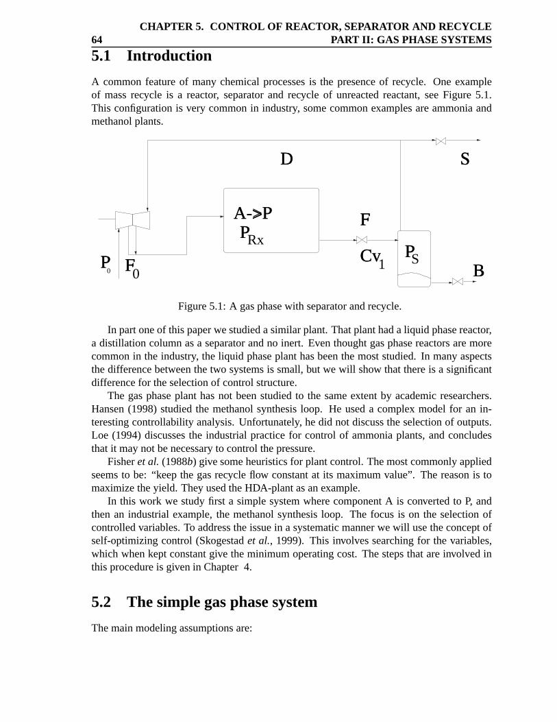
64CHAPTER 5. CONTROL OF REACTOR, SEPARATOR AND RECYCLE
PART II: GAS PHASE SYSTEMS
5.1 Intr oduction
A commonfeatureof many chemicalprocessesis the presenceof recycle. Oneexampleof massrecycle is a reactor, separatorand recycle of unreactedreactant,seeFigure 5.1.This configurationis very commonin industry, somecommonexamplesareammoniaandmethanolplants.
0P
P
D
F
B
S
Cv P
A->P
F0
Rx
1 S
Figure5.1: A gasphasewith separatorandrecycle.
In partoneof thispaperwestudiedasimilarplant.Thatplanthada liquid phasereactor,a distillation columnasa separatorandno inert. Eventhoughtgasphasereactorsaremorecommonin the industry, the liquid phaseplanthasbeenthemoststudied.In many aspectsthedifferencebetweenthetwo systemsis small,but we will show thatthereis a significantdifferencefor theselectionof controlstructure.
The gasphaseplant hasnot beenstudiedto the sameextent by academicresearchers.Hansen(1998)studiedthe methanolsynthesisloop. He useda complex model for an in-terestingcontrollability analysis.Unfortunately, hedid not discusstheselectionof outputs.Loe (1994)discussesthe industrialpracticefor control of ammoniaplants,andconcludesthatit maynot benecessaryto controlthepressure.
Fisheret al. (1988b) givesomeheuristicsfor plantcontrol.Themostcommonlyappliedseemsto be: “keepthe gasrecycle flow constantat its maximumvalue”. The reasonis tomaximizetheyield. They usedtheHDA-plantasanexample.
In this work we studyfirst a simplesystemwherecomponentA is convertedto P, andthenan industrialexample,the methanolsynthesisloop. The focus is on the selectionofcontrolledvariables.To addresstheissuein a systematicmannerwewill usetheconceptofself-optimizingcontrol (Skogestadet al., 1999). This involvessearchingfor the variables,which whenkeptconstantgive theminimumoperatingcost. Thestepsthatareinvolvedinthis procedureis givenin Chapter4.
5.2 The simplegasphasesystem
Themainmodelingassumptionsare:
5.2. THE SIMPLE GAS PHASE SYSTEM 65
À Isothermalreactor(noenergy balance).
À Sharpsplit in the separator, reactantS andinert in the gasphaseareseparatedfromtheliquid product � .
À Idealgaslaw.
À Thereactionrateof SÁ� � is givenby QRHMF�EGF , where EGF is themolarholdupin thereactor, HMF is thecompositionof S in thereactorand Q is thereactionrate.
À Thereactoreffluentflow to theseparatoris drivenby thepressuredifference,i.e. B`^Â¬Ã·Ä Å �¦ÆFÈÇ b®�²ÆZ Å . Where �ÉFÈÇ is reactorpressureand �DZ is separatorpressure.This isassumedto betheonly pressuredropin theloop.
À Thecompressorwork is modeledasisothermalidealgascompression.
À Thecompressorsaremountedon a commonshaft.This is impliesthat ÊËFgÌYÍ$Î�Í$Ï�ÌÐO·ÊËÑmÒ�ÓÕÔis constant,whereÊ is themolarwork of eitherthemainor recyclecompressor.
Wehaveassumedthatboththefeedflow rate BDC andup-streampressure�DC areindependentvariables(disturbances).This is not really possible,sincea changesin BDC mustbefollowedby achangein pressure�LC (thepressure�DC representssomelocalup-steamgashold-up).Soimplicitly we haveassumedthatthereis a controlsystemin place(i.e. themaincompressoris adjustedto keep �LC constant).
Step 1: Degreesof fr eedom We have assumedthat feedrateandup-streampressure�DCis given,this implies that themaincompressorwork is givenandthereforealsotherecyclecompressorwork (commonshaft). Sinceany valvesin the loop shouldbe fully open,weonly have two manipulatedvariables.Oneof these,« , is usedto control the liquid level intheseparator. Thereis onedegreeof freedomat steadystate.
Step 2: The objective function The goal of operationis to maximizethe valuesof theproductstreamdiminishedby the value of feed streamsand utility costs. For the liquidphaseplanttherewasonly onefeedandonly oneexit stream,henceduringtheoptimizationweneedonly to minimizethecostof utility. However for thegasphasesystemwehave twoproductflows with differentprice.Theobjective functionto bemaximizedis then
T¾^¢Ö2K׫�Ø�Ö2Ù¼Ú©b¹ÖÛ¶ÜyBLCPb¹Ý°Þ�ßáà(ßYÞ�â (5.1)
Where « is theproductflow, Ú is thepurgeflow, BDC is the feedrate. Using the total massbalance,Ú¨^ãBDC-b®« gives
T¡^äWáÖK¾b¹Ö2Ù¼[Ы`bãWYÖÛ¶Ü_b¹Ö2Ù¼[ÐBDC-b�Ý°Þ�ßáà(ßYÞ�â (5.2)
BDC is givenandmayberemovedform theobjective. Theutility is compressorwork, intro-ductionof a relativecostgives:
T¾^�«`b½ÊËFÉWáå � Øæå Æ [ (5.3)
66CHAPTER 5. CONTROL OF REACTOR, SEPARATOR AND RECYCLE
PART II: GAS PHASE SYSTEMS
where ÊËF is therelative costof compressorworkscomparedto ÖK©b�Ö2Ù . å � and å Æ com-pressorwork is
å � ^çBDC6èêé¡ë4ì �ÉF�LC (5.4)
Unlike theliquid phasesystem,thereis apenaltyfor increasingthehold-up(pressure)in thereactor. If theupstreampressureis higherthan �LF thentherewould beno needfor themaincompressorandthis termwouldvanish.Therecyclecompressorwork is givenby
å Æ ^ �tèêé¡ë&ì �LF�mÙ (5.5)
^ �tèêé¡ë&ì �LF�LF¸b®í:�
From this equationwe seethat the pressuredrop shouldbe assmall aspossible,thusanyunnecessarypressuredropshouldbeavoided(fully openvalve). Furthermoreasthereactorpressureis increased,this termwill decrease.Very often it will be negligible comparedtothemain-compressorwork. Therewill only beasmallincentivefor anindependentshaftforthecompressors.They areoftenmountedon a commonshaft,which will bethecasein thisstudy(seesection5.3.3).
The last term in 5.3 representsthe valuableproduct. Henceit shouldbe as large aspossible.Productionratecanbe increasedby increasingthe reactorpressureandtherebydecreasingthe purge. This gives an increasein compressorwork, the optimum may beunconstrained.
Step3: Disturbances Weassumethatthroughputis themaindisturbancehere: BLCË^î���e�e�mole/s £¤�2�e¥ .
Step4: Optimization Figure5.2 shows thecontributionsto theobjective function T . Aspurgeflow is reduced,we producemorevaluableproduct.But thepressureandcompressorwork increases.At full conversion,thereactorpressureandcompressorwork wouldbecomeinfinite.
In Figure5.2(c),theobjectivehasbeenplottedfor severalrelativecostsÊËF (i.e. rangingfrom 0 to 4 mole/MJ.It showshow theoptimumwouldmovetowardslowerpurgeandhigherconversionif therelativeweightwerereducedsothatcompressorcostsareless.If ÊËF is lowenoughthe optimum will be constrained,either by maximumpressureor by compressorload. We will studyanunconstrainedcase,with a relative weight ÊËF§^�� mole/MJ,markedwith ax in Figure 5.2(c).
Step5: Candidatesfor control Our candidatesfor theremainingdegreeof freedomare:purgeflow Ú , recycle flow è , purgeflow fraction Ú×O2è , inert compositionin recycle ï�ð andreactorpressure�LF .
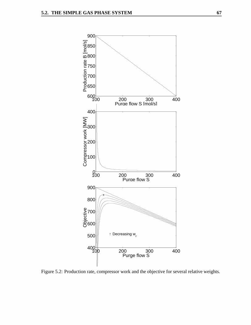
5.2. THE SIMPLE GAS PHASE SYSTEM 67
100 200 300 400600
650
700
750
800
850
900
Purge flow S [mol/s]
Pro
duct
ion
rate
B [m
ol/s
]
100 200 300 4000
100
200
300
400
Purge flow S
Com
pres
sor
wor
k [M
W]
100 200 300 400400
500
600
700
800
900
Purge flow S
Obj
ectiv
e
x
↑ Decreasing wr
Figure5.2: Productionrate,compressorwork andtheobjective for severalrelativeweights.
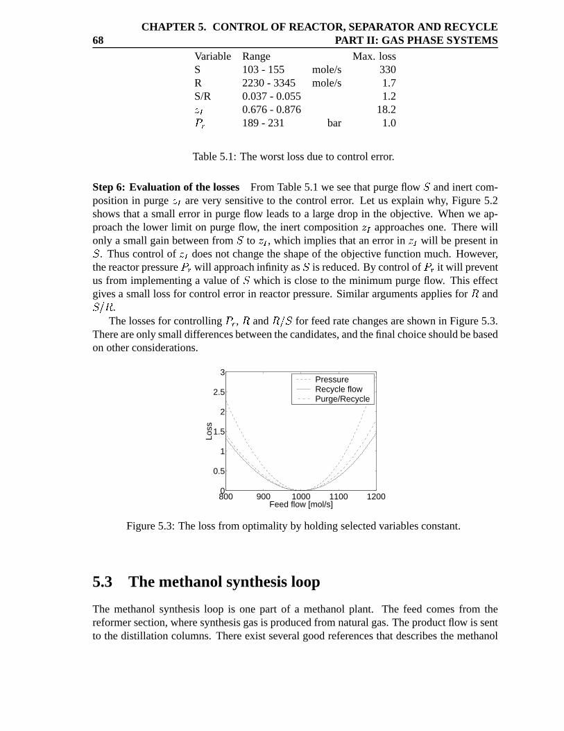
68CHAPTER 5. CONTROL OF REACTOR, SEPARATOR AND RECYCLE
PART II: GAS PHASE SYSTEMS
Variable Range Max. lossS 103- 155 mole/s 330R 2230- 3345 mole/s 1.7S/R 0.037- 0.055 1.2ï�ð 0.676- 0.876 18.2�LF 189- 231 bar 1.0
Table5.1: Theworstlossdueto controlerror.
Step6: Evaluation of the losses FromTable5.1we seethatpurgeflow Ú andinert com-positionin purge ï�ð arevery sensitive to the control error. Let us explain why, Figure5.2shows thata small error in purgeflow leadsto a large drop in theobjective. Whenwe ap-proachthe lower limit on purge flow, the inert compositionï�ð approachesone. Therewillonly a smallgainbetweenfrom Ú to ï�ð , which impliesthatanerror in ï�ð will bepresentinÚ . Thuscontrolof ï�ð doesnot changetheshapeof theobjective functionmuch. However,thereactorpressure�LF will approachinfinity as Ú is reduced.By controlof �LF it will preventus from implementinga valueof Ú which is closeto theminimumpurge flow. This effectgivesa small lossfor controlerror in reactorpressure.Similar argumentsappliesfor è andÚ×O2è .
Thelossesfor controlling �LF , è and è²O2Ú for feedratechangesareshown in Figure5.3.Thereareonly smalldifferencesbetweenthecandidates,andthefinal choiceshouldbebasedon otherconsiderations.
800 900 1000 1100 12000
0.5
1
1.5
2
2.5
3
Feed flow [mol/s]
Loss
Pressure Recycle flow Purge/Recycle
Figure5.3: Thelossfrom optimality by holdingselectedvariablesconstant.
5.3 The methanol synthesisloop
The methanolsynthesisloop is one part of a methanolplant. The feed comesfrom thereformersection,wheresynthesisgasis producedfrom naturalgas.Theproductflow is sentto thedistillation columns.Thereexist severalgoodreferencesthatdescribesthemethanol
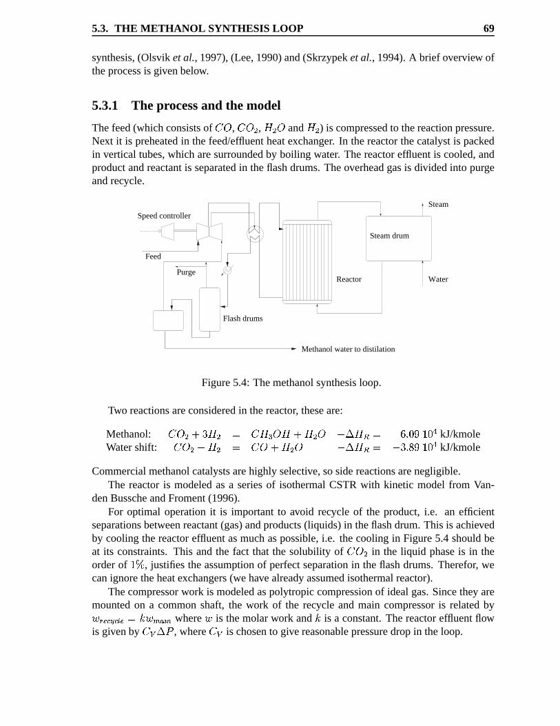
5.3. THE METHANOL SYNTHESIS LOOP 69
synthesis,(Olsvik etal., 1997),(Lee,1990)and(Skrzypeketal., 1994).A brief overview oftheprocessis givenbelow.
5.3.1 The processand the model
Thefeed(whichconsistsof¤ñ
,¦ñ Æ , ò Æ ñ and ò Æ ) is compressedto thereactionpressure.
Next it is preheatedin thefeed/effluentheatexchanger. In thereactorthecatalystis packedin verticaltubes,which aresurroundedby boiling water. Thereactoreffluentis cooled,andproductandreactantis separatedin theflashdrums.Theoverheadgasis dividedinto purgeandrecycle.
Water
Steam drum
Methanol water to distilation
Steam
Speed controller
Flash drums
ReactorPurge
Feed
Figure5.4: Themethanolsynthesisloop.
Two reactionsareconsideredin thereactor, theseare:
Methanol:¦ñ Æ Ø¹�eò Æ ^  ò:ó ñ ò�Øæò Æ ñ b°í0ò:ô�^ õ"�ö�eµ¤�¶�÷ kJ/kmole
Watershift:¦ñ Æ Øæò Æ ^ ¦ñ Øæò Æ ñ b°í0ò:ô�^ bê�"�ö�eµ¤�¶�÷ kJ/kmole
Commercialmethanolcatalystsarehighly selective,sosidereactionsarenegligible.The reactoris modeledasa seriesof isothermalCSTRwith kinetic model from Van-
denBusscheandFroment(1996).For optimal operationit is importantto avoid recycle of the product,i.e. an efficient
separationsbetweenreactant(gas)andproducts(liquids) in theflashdrum.This is achievedby coolingthereactoreffluentasmuchaspossible,i.e. thecooling in Figure5.4 shouldbeat its constraints.This andthe fact that the solubility of
¤ñ Æ in the liquid phaseis in theorderof �v¥ , justifiestheassumptionof perfectseparationin theflashdrums.Therefor, wecanignoretheheatexchangers(wehavealreadyassumedisothermalreactor).
Thecompressorwork is modeledaspolytropiccompressionof idealgas.Sincethey aremountedon a commonshaft, the work of the recycle andmain compressoris relatedbyÊËFgÌáÍ(Î�Í$Ï�ÌË^äQ"ÊËÑDÒÐÓöÔ where Ê is themolarwork and Q is a constant.Thereactoreffluentflowis givenby
ªø í:� , whereªø
is chosento givereasonablepressuredropin theloop.
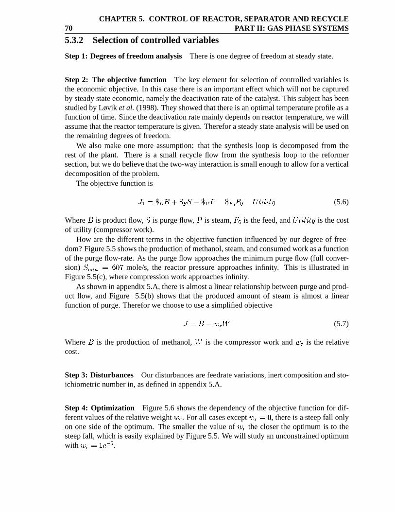
70CHAPTER 5. CONTROL OF REACTOR, SEPARATOR AND RECYCLE
PART II: GAS PHASE SYSTEMS
5.3.2 Selectionof controlled variables
Step1: Degreesof fr eedomanalysis Thereis onedegreeof freedomat steadystate.
Step 2: The objective function The key elementfor selectionof controlledvariablesistheeconomicobjective. In this casethereis an importanteffect which will not becapturedby steadystateeconomic,namelythedeactivationrateof thecatalyst.Thissubjecthasbeenstudiedby Løvik etal. (1998).They showedthatthereis anoptimaltemperatureprofileasafunctionof time. Sincethedeactivationratemainlydependson reactortemperature,wewillassumethatthereactortemperatureis given.Thereforasteadystateanalysiswill beusedontheremainingdegreesof freedom.
We alsomake onemore assumption:that the synthesisloop is decomposedfrom therest of the plant. There is a small recycle flow from the synthesisloop to the reformersection,but wedobelievethatthetwo-wayinteractionis smallenoughto allow for averticaldecompositionof theproblem.
Theobjective functionis
T � ^¢ÖK׫çØæÖ2Ù¼Ú¡ØæÖù×��b¹Ö·Û¶ÜyBDC-bæÝ»Þ�ßÈà(ßaÞ�â (5.6)
Where « is productflow, Ú is purgeflow, � is steam,BDC is thefeed,and Ý»Þ�ßÈà(ßaÞ�â is thecostof utility (compressorwork).
How arethe differenttermsin the objective function influencedby our degreeof free-dom?Figure5.5showstheproductionof methanol,steam,andconsumedwork asafunctionof thepurgeflow-rate.As thepurgeflow approachestheminimumpurgeflow (full conver-sion) ÚúÑLÓÕÔã^ õe��û mole/s, the reactorpressureapproachesinfinity. This is illustratedinFigure5.5(c),wherecompressionwork approachesinfinity.
As shown in appendix5.A, thereis almosta linearrelationshipbetweenpurgeandprod-uct flow, and Figure 5.5(b) shows that the producedamountof steamis almosta linearfunctionof purge.Thereforwechooseto useasimplifiedobjective
T¾^�«`b½ÊËF6å (5.7)
Where « is the productionof methanol,å is the compressorwork and ÊËF is the relativecost.
Step3: Disturbances Our disturbancesarefeedratevariations,inert compositionandsto-ichiometricnumberin, asdefinedin appendix5.A.
Step4: Optimization Figure5.6 shows thedependency of theobjective functionfor dif-ferentvaluesof therelativeweight ÊËF . For all casesexcept ÊËFP^ç� , thereis asteepfall onlyon onesideof the optimum. The smallerthe valueof ÊËF the closerthe optimumis to thesteepfall, which is easilyexplainedby Figure5.5.Wewill studyanunconstrainedoptimumwith ÊËF¬^`�¶ü �Rý .
5.3. THE METHANOL SYNTHESIS LOOP 71
800 1000 1200 1400 1600600
650
700
750
800
850
900
Purge flow [mol/s]
Pro
duct
ion
of C
H3O
H [m
ol/s
]
800 1000 1200 1400 1600
1.15
1.2
1.25
1.3
1.35
1.4
1.45x 10
8
Purge flow [mol/s]
Ste
am [J
/s]
600 800 1000 1200 1400 1600
1
1.5
2
2.5
3
3.5
x 107
Purge flow [mol/s]
Com
pres
sor
wor
k [J
/s]
Figure5.5: Productionrate,steamproductionandtheobjective.
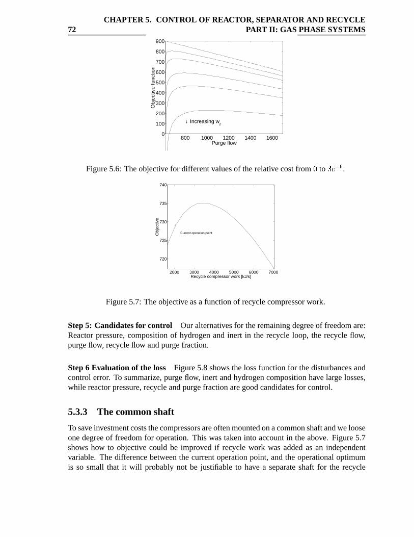
72CHAPTER 5. CONTROL OF REACTOR, SEPARATOR AND RECYCLE
PART II: GAS PHASE SYSTEMS
800 1000 1200 1400 16000
100
200
300
400
500
600
700
800
900
Purge flow
Obj
ectiv
e fu
nctio
n
↓ Increasing wr
Figure5.6: Theobjective for differentvaluesof therelativecostfrom þ to ÿ���� � .
2000 3000 4000 5000 6000 7000
720
725
730
735
740
Recycle compressor work [kJ/s]
Obj
ectiv
e
Current operation point
Figure5.7: Theobjectiveasa functionof recyclecompressorwork.
Step5: Candidatesfor control Our alternativesfor theremainingdegreeof freedomare:Reactorpressure,compositionof hydrogenandinert in the recycle loop, the recycle flow,purgeflow, recycleflow andpurgefraction.
Step6 Evaluation of the loss Figure5.8shows thelossfunctionfor thedisturbancesandcontrolerror. To summarize,purgeflow, inert andhydrogencompositionhave large losses,while reactorpressure,recycleandpurgefractionaregoodcandidatesfor control.
5.3.3 The commonshaft
To saveinvestmentcoststhecompressorsareoftenmountedonacommonshaftandwelooseonedegreeof freedomfor operation.This wastaken into accountin theabove. Figure5.7shows how to objective could be improved if recycle work wasaddedasan independentvariable. Thedifferencebetweenthecurrentoperationpoint, andtheoperationaloptimumis so small that it will probablynot be justifiable to have a separateshaft for the recycle
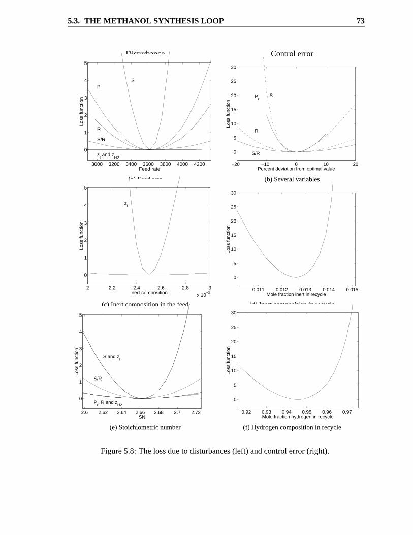
5.3. THE METHANOL SYNTHESIS LOOP 73
Disturbance Controlerror
3000 3200 3400 3600 3800 4000 4200
0
1
2
3
4
5
Feed rate
Loss
func
tion
SP
r
R
S/R
zI and z
H2
(a)Feedrate
−20 −10 0 10 20
0
5
10
15
20
25
30
Percent deviation from optimal value
Loss
func
tion
S/R
SPr
R
(b) Severalvariables
2 2.2 2.4 2.6 2.8 3
x 10−3
0
1
2
3
4
5
Inert composition
Loss
func
tion
zI
(c) Inert compositionin thefeed
0.011 0.012 0.013 0.014 0.015
0
5
10
15
20
25
30
Mole fraction inert in recycle
Loss
func
tion
(d) Inert compositionin recycle
2.6 2.62 2.64 2.66 2.68 2.7 2.72
0
1
2
3
4
5
SN
Loss
func
tion
Pr, R and z
H2
S/R
S and zI
(e)Stoichiometricnumber
0.92 0.93 0.94 0.95 0.96 0.97
0
5
10
15
20
25
30
Mole fraction hydrogen in recycle
Loss
func
tion
(f) Hydrogencompositionin recycle
Figure5.8: Thelossdueto disturbances(left) andcontrolerror(right).
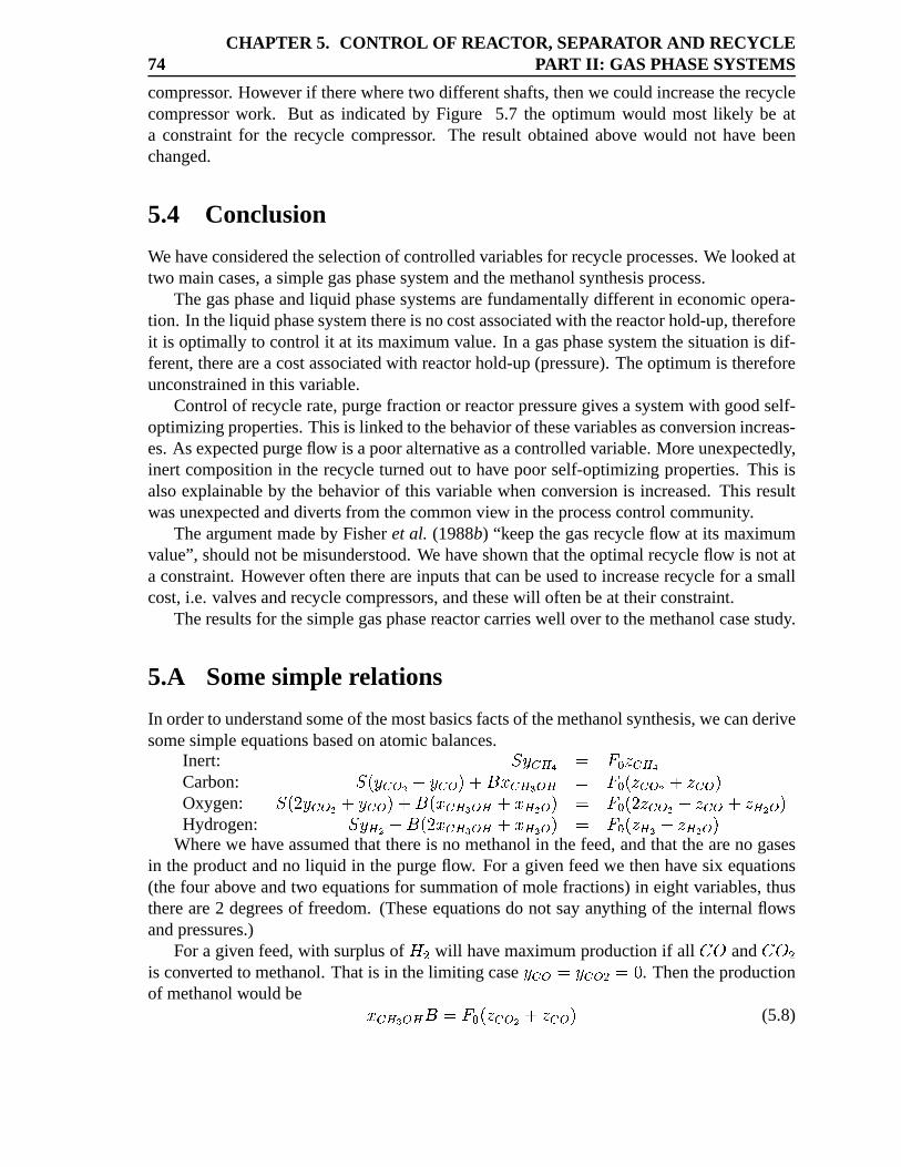
74CHAPTER 5. CONTROL OF REACTOR, SEPARATOR AND RECYCLE
PART II: GAS PHASE SYSTEMS
compressor. However if therewheretwo differentshafts,thenwecouldincreasetherecyclecompressorwork. But as indicatedby Figure 5.7 the optimum would most likely be ata constraintfor the recycle compressor. The result obtainedabove would not have beenchanged.
5.4 Conclusion
Wehaveconsideredtheselectionof controlledvariablesfor recycleprocesses.We lookedattwo maincases,asimplegasphasesystemandthemethanolsynthesisprocess.
Thegasphaseandliquid phasesystemsarefundamentallydifferentin economicopera-tion. In theliquid phasesystemthereis nocostassociatedwith thereactorhold-up,thereforeit is optimally to control it at its maximumvalue. In a gasphasesystemthesituationis dif-ferent,therearea costassociatedwith reactorhold-up(pressure).Theoptimumis thereforeunconstrainedin this variable.
Controlof recycle rate,purgefractionor reactorpressuregivesa systemwith goodself-optimizingproperties.This is linkedto thebehavior of thesevariablesasconversionincreas-es.As expectedpurgeflow is apooralternativeasacontrolledvariable.Moreunexpectedly,inert compositionin the recycle turnedout to have poorself-optimizingproperties.This isalsoexplainableby the behavior of this variablewhenconversionis increased.This resultwasunexpectedanddivertsfrom thecommonview in theprocesscontrolcommunity.
Theargumentmadeby Fisheret al. (1988b) “keepthegasrecycle flow at its maximumvalue”,shouldnot bemisunderstood.We have shown thattheoptimalrecycle flow is not ata constraint.However oftenthereareinputsthatcanbeusedto increaserecycle for a smallcost,i.e. valvesandrecyclecompressors,andthesewill oftenbeat their constraint.
Theresultsfor thesimplegasphasereactorcarrieswell over to themethanolcasestudy.
5.A Somesimple relations
In orderto understandsomeof themostbasicsfactsof themethanolsynthesis,wecanderivesomesimpleequationsbasedonatomicbalances.
Inert:������� ���������
Carbon:������������������� �"!$#���%&�� �����'����(�)�"���� �
Oxygen:���'*�����(� �+���������!,�-#���%&�./�+#���0��� �����1*�����(�)������2����3�0���
Hydrogen:�4��3� ��!,�1*5#���%&�./�+#���0��� �����'��3�)����3�0� �
Wherewe have assumedthat thereis no methanolin thefeed,andthat theareno gasesin theproductandno liquid in thepurgeflow. For a givenfeedwe thenhave six equations(thefour above andtwo equationsfor summationof molefractions)in eightvariables,thusthereare2 degreesof freedom.(Theseequationsdo not sayanything of the internalflowsandpressures.)
For a givenfeed,with surplusof 687 will have maximumproductionif all 9;: and 9$:<7is convertedto methanol.Thatis in thelimiting case
����= >���� 7 þ . Thentheproductionof methanolwouldbe #�� % �.?!@ >�)�5�'���� � �"���� �
(5.8)
5.4. CONCLUSION 75
Theminimumamountof hydrogenin thepurgeflow������? >���A������(�)�"���� �B�'�4CED�*��(5.9)
Wherethestoichiometricnumberis definedas�4CF G ���H � G ��(�-HG ���HJI G ��(�KH . Which togetherwith the
amountof inertgivestheminimumpurgeflow�L M�)�5�'�����N�>�'����(� ������ �B�'�OCPD+*��Q�(5.10)
If�OCR S*
thenwewill losenohydrogenin thepurgefor full conversion.What theseequationtells us is obvious,for a givenfeedthereis anupperlimit for pro-
ducedmethanolwhich is givenby the amountof carbonin the feed. And thereis a lowerlimit for purge gas,which is given by the amountof inert andsurplusof hydrogenin thefeed.
Purgeflow is relatedto feedflow andproductflow by (from a totalmolebalance)�T M���OD+!,� ÿ #���%&�./�U#�3�0���(5.11)

Chapter 6
Selectionof controlled variablesfor the TennesseeEastmanproblem
T. Larsson,K. HestetunandS.Skogestad
Abstract
Thischapteraddressestheselectionof controlledvariables,thatis, “what shouldwecontrol”. Theconceptof self-optimizingcontrolprovidesasystematictool for this,andin thepaperweshow how it maybeappliedtotheTennesseeEastmanprocess,whichhasa very largenumberof candidatevariables.In thepaperwepresenta systematicprocedurefor reducingthenumberof alternatives.Onestepis to eliminatevariables,which withconstantsetpointsresultin largelossesor infeasibilitywhentherearedisturbances(with theremainingdegreesof freedomreoptimized).
Thefollowing controlledvariablesarerecommendedfor this problem:V Equalityconstrainedvariables:Productcompositionandproduct-rate.(Wehavenotassignedmeasure-mentsor manipulatedvariablesto these.)V Optimally constrainedvariables: Reactorlevel, reactorpressure,compressorrecycle valve, strippersteamvalveandagitatorspeed.V Unconstrainedvariableswith goodself-optimizingproperties:Reactortemperature,compositionof Cin purgeandrecycleflow or compressorwork.
A commonsuggestionis to control the inventoryof inert components.However, this is a poorchoicefor this
problem,sinceanunfavorableshapeof theeconomicobjective function implies thata smallerrorcanleadto
infeasibility. Thus,werecommendleetinginertcompositionfloat.
78CHAPTER 6. SELECTION OF CONTROLLED VARIABLES
FOR THE TENNESSEEEASTMAN PROBLEM
6.1 Intr oduction
Thispaperaddressestheselectionof controlledvariablesfor theTennesseeEastmanprocess.Webasetheselectionontheconceptof self-optimizingcontrolusingsteadystatemodelsandsteadystateeconomics.
“Self-optimizingcontrol” is whenanacceptable(economic)losscanbeachievedusingconstantsetpointsfor thecontrolledvariables,without theneedto reoptimizewhendistur-bancesoccur(Morari etal., 1980),(Skogestad,2000).Theconstantsetpointpolicy is simple,but it will notbeoptimal(andthushaveapositive loss)dueto thefollowing two factors
1. Disturbances,i.e. changesin (independent)variablesandparameterscomparedto theirnominalvalues,which causetheoptimalsetpointsto change.
2. Implementationerrors,i.e. differencesbetweenthesetpointsandtheactualvaluesofthecontrolledvariables(e.g. dueto measurementerrorsor poorcontrol) (Skogestad,2000).
Theeffect of thesefactors(the loss)dependson thechoiceof controlledvariables,andtheobjective is to find asetof controlledvariablesfor which thelossis acceptable.
Downs and Vogel (1993) introducedthe TennesseeEastmanchallengeproblemat anAIChE meetingin 1990.Thepurposewasto supplytheacademicswith aproblemthatcon-tainedmany of the challengesthat peoplein industrymeet. Thereareeight components,includinganinert (B) anda byproduct(F). ThereactionsareA(g) + C(g) + D(g) W G(liq) (Product)A(g) + C(g) + E(g) W H(liq) (Product)
A(g) + E(g) W F(liq) (Byproduct)3D(g) W 2F(liq) (Byproduct)
The processhasfour feedstreams(of A, D, E andA+C), oneproductstreamandonepurgestream.Theinert (B) entersin theA+C feedstream.Theprocesshasfivemajorunits;a reactor, a productcondenser, a vapor-liquid separator, a recycle compressoranda productstripper, seeFigure 6.1. Thereare 41 measurementsand 12 manipulatedvariables. Weherestudytheoptimaloperationof thebasecase(mode1) with a given50/50productratiobetweencomponentsG andH, andagivenproductionrate.
This plant hasbeenstudiedby many authors,andit hasbeenimportantfor the devel-opmentof plantwidecontrol as a field. Many authorshave usedit to demonstratetheirprocedurefor thedesignof a controlsystem,e.g. seeChapter2 for a review of thevariousapproaches.Wehereonly considertheselectionof controlledvariables.
McAvoy andYe (1994)selectthecontrolledvariablesin a somewhatad hoc fashion.Inadditionto theliquid levels,they controlreactortemperature,reactorpressure,recycle flowrate,compressorwork, concentrationof B (inert) in purge, concentrationof E in productflow.
LymanandGeorgakis(1995)recommenda control structurewherethe following vari-ablesare controlled: Reactortemperature,reactorlevel, recycle flow rate, agitationrate,compositionof A, D andE in reactorfeed,compositionof B (inert) in purgeandcomposi-tion of E in product.Eventhoughthey considertheoperationcostfor thecontrolstructure,
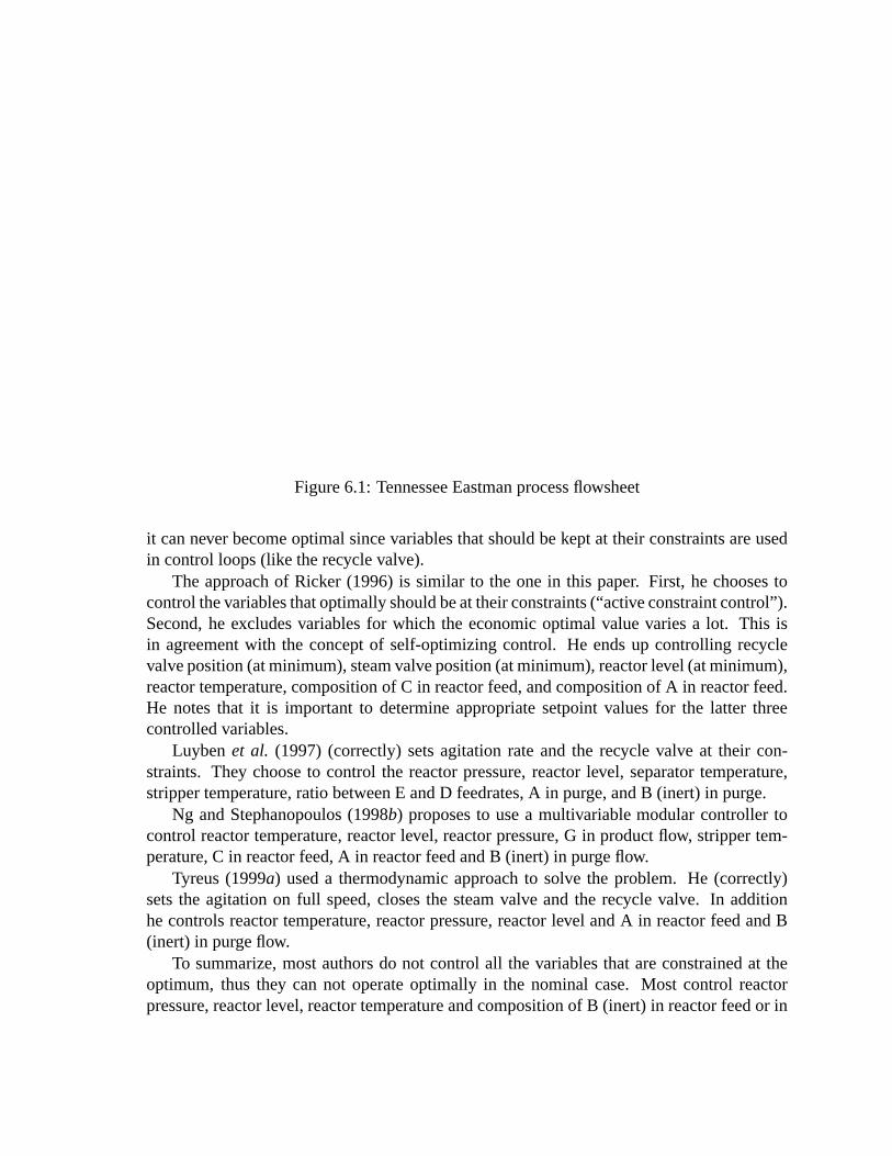
6.1. INTRODUCTION 79
Stm
FI
TI
Reactor
TIFI
XA
XB
XC
XD
XF
XE
E
D
A
SC
LI
CWS
CWR
CWS
CWR
TI
FI
C
Cond
Product
FI
TI
LI
FI
Purge
FI
PI
JI Compressor
XA
XB
XC
XD
XF
XE
XG
XH
XD
XF
XE
ANALYZER
XG
XH
Vap/Liq
StripperSeparator
Condenser
1
2
3
6
4
7
12
5
8
10
11
9
LI
PI
FI
FI
FI
FI
ANALYZER
ANALYZER
PI
TI
y1
y2
y3
y4
u4
u2
u1
u3
y6
y8
u12
y7
y21
y9
u10
u11
y22
y20
y5 u5
y10
u6
y13
y12
y11y14
u7
y18
y16
y15
y17
u8
u9
y19
y3
y23
y24
y25
y26
y27
y28
y29
y30
y31
y32
y33
y34
y35
y36
y37
y38
y39
y40
y41
(y1)(y2)
(y3)
(y4)
(y5)(y6)
(y7)
(y8)
(y9)
(y10)
(y11)
Figure6.1: TennesseeEastmanprocessflowsheet
it cannever becomeoptimalsincevariablesthatshouldbekeptat their constraintsareusedin controlloops(like therecyclevalve).
The approachof Ricker (1996) is similar to the onein this paper. First, he choosestocontrolthevariablesthatoptimallyshouldbeattheirconstraints(“activeconstraintcontrol”).Second,he excludesvariablesfor which the economicoptimal valuevariesa lot. This isin agreementwith the conceptof self-optimizingcontrol. He endsup controlling recyclevalveposition(atminimum),steamvalveposition(atminimum),reactorlevel (atminimum),reactortemperature,compositionof C in reactorfeed,andcompositionof A in reactorfeed.He notesthat it is important to determineappropriatesetpointvaluesfor the latter threecontrolledvariables.
Luybenet al. (1997) (correctly) setsagitationrate and the recycle valve at their con-straints. They chooseto control the reactorpressure,reactorlevel, separatortemperature,strippertemperature,ratio betweenE andD feedrates,A in purge,andB (inert) in purge.
Ng andStephanopoulos(1998b) proposesto usea multivariablemodularcontroller tocontrol reactortemperature,reactorlevel, reactorpressure,G in productflow, strippertem-perature,C in reactorfeed,A in reactorfeedandB (inert) in purgeflow.
Tyreus(1999a) useda thermodynamicapproachto solve the problem. He (correctly)setsthe agitationon full speed,closesthe steamvalve and the recycle valve. In additionhecontrolsreactortemperature,reactorpressure,reactorlevel andA in reactorfeedandB(inert) in purgeflow.
To summarize,mostauthorsdo not control all the variablesthat areconstrainedat theoptimum, thus they can not operateoptimally in the nominal case. Most control reactorpressure,reactorlevel, reactortemperatureandcompositionof B (inert) in reactorfeedor in
80CHAPTER 6. SELECTION OF CONTROLLED VARIABLES
FOR THE TENNESSEEEASTMAN PROBLEM
purge. It is commonto controlstrippertemperature,separatortemperature,andcompositionof C and/orA in reactorfeed.
6.2 Stepwiseprocedure for self-optimizing control
We will apply thestepwiseprocedurefor self-optimizingcontrolof Skogestad(2000). Themainstepsare
1. Degreeof freedomanalysis
2. Definitionof optimaloperation(costandconstraints)
3. Identificationof importantdisturbances
4. Optimization
5. Identificationof candidatecontrolledvariables
6. Evaluationof thelosswith constantsetpointsfor thealternativecombinationsof con-trolledvariables(causedby disturbancesor implementationerrors)
7. Final evaluationandselection(includingcontrollability analysis)
In the earlierChapters,therewasonly oneunconstraineddegreeof freedom,so the eval-uation in step6 wasmanageable.However, for the TennesseeEastmanprocesstherearethreeunconstraineddegreesof freedom,so it is necessaryto do somemoreeffort in step5to reducethenumberof alternatives.We presentbelow somegeneralcriteriathatareusefulfor eliminatingcontrolledvariables.
6.3 Degreesof fr eedomanalysisand optimal operation
Theprocesshas12 manipulatedvariables,41 measurementsand20 disturbances.In addi-tion, all the manipulatedvariableshave constraintsandthereare“output” constraints,in-cludingequalityconstraintson productquality andproductrate.
DownsandVogel (1993)specifytheeconomiccost X [$/h] for theprocess,which is tobeminimized.In words,X Y�'Z-[�\A\�[�]_^�`ba"cd`�e � ^5fg`hZ�\�f'i$jk.^Al � `hi3mnj^�[5mbk�opeq\A�r� (6.1)�1\Be � `bcsot[�\Beq\A���M�'ou[Acvj^ � \A\wfg[Aixou[�\weq\A�Thefirst termdominatesthecost.
An analysis,seeTable6.1,shows thatthereareeightdegreesof freedomat steadystatewhich may be usedfor steady-stateoptimization. Ricker (1995) solved the optimizationproblemusingthe costfunction of DownsandVogel (1993)andgivesa goodexplanationon whathappensat theoptimum.At theoptimumtherearefive activeconstraintsandtheseshouldbecontrolledto achieveoptimaloperation(at leastnominally).
This leavesthreeunconstraineddegreesof freedom,which we wantto selectsuchthataconstantsetpointspolicy resultsin anacceptableeconomicloss(self-optimizingcontrol).
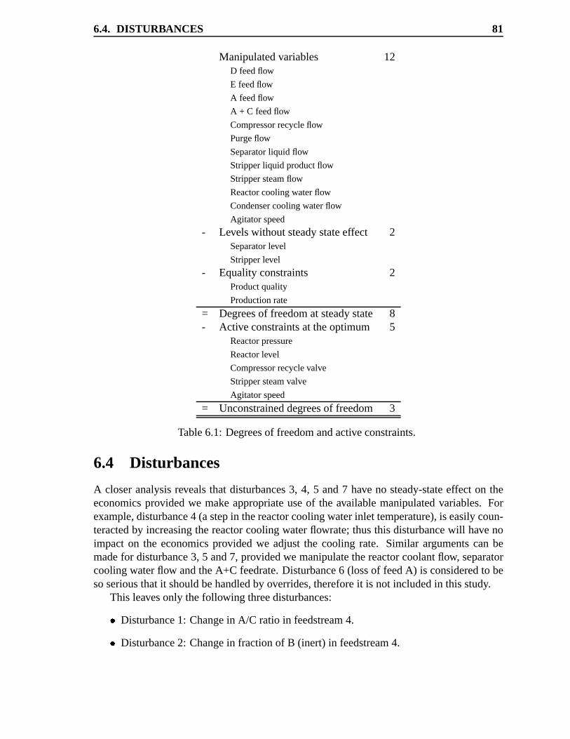
6.4. DISTURBANCES 81
Manipulatedvariables 12D feedflow
E feedflow
A feedflow
A + C feedflow
Compressorrecycleflow
Purgeflow
Separatorliquid flow
Stripperliquid productflow
Strippersteamflow
Reactorcoolingwaterflow
Condensercoolingwaterflow
Agitator speed
- Levelswithoutsteadystateeffect 2Separatorlevel
Stripperlevel
- Equalityconstraints 2Productquality
Productionrate
= Degreesof freedomat steadystate 8- Activeconstraintsat theoptimum 5
Reactorpressure
Reactorlevel
Compressorrecyclevalve
Strippersteamvalve
Agitator speed
= Unconstraineddegreesof freedom 3
Table6.1: Degreesof freedomandactiveconstraints.
6.4 Disturbances
A closeranalysisrevealsthat disturbances3, 4, 5 and7 have no steady-stateeffect on theeconomicsprovided we make appropriateuseof the availablemanipulatedvariables. Forexample,disturbance4 (astepin thereactorcoolingwaterinlet temperature),is easilycoun-teractedby increasingthereactorcoolingwaterflowrate;thusthis disturbancewill have noimpact on the economicsprovided we adjustthe cooling rate. Similar argumentscan bemadefor disturbance3, 5 and7, providedwe manipulatethereactorcoolantflow, separatorcoolingwaterflow andtheA+C feedrate.Disturbance6 (lossof feedA) is consideredto besoseriousthatit shouldbehandledby overrides,thereforeit is not includedin this study.
This leavesonly thefollowing threedisturbances:y Disturbance1: Changein A/C ratio in feedstream4.y Disturbance2: Changein fractionof B (inert) in feedstream4.
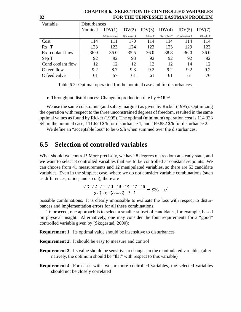
82CHAPTER 6. SELECTION OF CONTROLLED VARIABLES
FOR THE TENNESSEEEASTMAN PROBLEM
Variable DisturbancesNominal IDV(1) IDV(2) IDV(3) IDV(4) IDV(5) IDV(7)
A/C in stream4 B in stream4 D feedT Rx coolantT CondcoolantT C headerP
Cost 114 111 170 114 114 114 114Rx. T 123 123 124 123 123 123 123Rx. coolantflow 36.0 36.0 35.5 36.0 38.8 36.0 36.0SepT 92 92 93 92 92 92 92Condcoolantflow 12 12 12 12 12 14 12C feedflow 9.2 8.7 9.3 9.2 9.2 9.2 9.2C feedvalve 61 57 61 61 61 61 76
Table6.2: Optimaloperationfor thenominalcaseandfor disturbances.y Throughputdisturbances:Changein productionrateby z|{A} %.
Weusethesameconstraints(andsafetymargins)asgivenby Ricker (1995).Optimizingtheoperationwith respectto thethreeunconstraineddegreesof freedom,resultedin thesameoptimalvaluesasfoundby Ricker (1995).Theoptimal(minimum)operationcostis 114.323$/h in thenominalcase,111.620$/h for disturbance1, and169.852$/h for disturbance2.
Wedefinean“acceptableloss” to be6 $/hwhensummedover thedisturbances.
6.5 Selectionof controlled variables
Whatshouldwe control?More precisely, we have 8 degreesof freedomat steadystate,andwe want to select8 controlledvariablesthatareto be controlledat constantsetpoints.Wecanchoosefrom 41 measurementsand12 manipulatedvariables,so thereare53 candidatevariables.Evenin thesimplestcase,wherewe do not considervariablecombinations(suchasdifferences,ratios,andsoon), thereare}2ÿ<~5} * ~5}�{�~5}2þ�~��b�<~��b��~��h��~������~���~A��~5}<~���~¶ÿ�~ * ~b{ �����<~b{¶þ��possiblecombinations.It is clearly impossibleto evaluatethe losswith respectto distur-bancesandimplementationerrorsfor all thesecombinations.
To proceed,oneapproachis to selecta smallersubsetof candidates,for example,basedon physical insight. Alternatively, one may considerthe four requirementsfor a “good”controlledvariablegivenby (Skogestad,2000):
Requirement1. Its optimalvalueshouldbeinsensitive to disturbances
Requirement2. It shouldbeeasyto measureandcontrol
Requirement3. Its valueshouldbesensitiveto changesin themanipulatedvariables(alter-natively, theoptimumshouldbe“flat” with respectto thisvariable)
Requirement4. For caseswith two or more controlledvariables,the selectedvariablesshouldnotbecloselycorrelated
6.5. SELECTION OF CONTROLLED VARIABLES 83
However, theserequirementsrequirequite a lot of effort with respectto optimization,andareat the sametime ratherqualitative. We thereforewant to find somemorequantitativecriteriafor eliminatingvariables,until weareleft with amanageablenumber.
Thefollowing criteriaareproposedto reducethenumberof alternatives. Most of themareratherobvious,but neverthelesswe find themuseful.
1. Active constraintcontrol: We chooseto control the active constraints.This reducesthenumberof controlledvariablesto beselected(in our casefrom 8 to 3). Of course,wemustalsoeliminatethecorrespondingvariablesfrom furtherconsideration.
2. Eliminatevariablesrelatedto equalityconstraints
3. Eliminatevariableswith noeffecton theeconomics(i.e. with no steady-stateeffect)
4. Eliminate/groupcloselyrelatedvariables
5. Processinsight: Eliminatefurthercandidates
6. Eliminatesinglevariableswhichwith constantsetpointsyield infeasibilityor largelosswhenthereare(1) disturbances(with theremainingdegreesof freedomreoptimized)or (2) implementationerrors.
7. Eliminate combinations(pairs, triplets, etc.) of variablesthat yield infeasibility orlargeloss
After this weenterinto thefinal evaluation:
8. Evaluationof disturbancelossfor remainingcombinations
9. Evaluationof implementationloss
6.5.1 Activeconstraint control
As mentioned,thereare5 active constraints.3 of the constraintsarerelatedto themanip-ulatedvariables(compressorrecycle, strippersteamandagitatorspeed);this eliminates3manipulatedvariablesand also 1 directly relatedmeasurement(strippersteam). 2 of theconstraintsarerelatedto outputs(reactorlevel andpressure);this eliminatesanother2 mea-surements.
We are now left with 38 measurementsand 9 manipulatedvariables,from which wewantto select3 unconstrainedcontrolledvariables.Thisgives16215possiblecombinations,which is still muchtoo large.
6.5.2 Eliminate variables relatedto equality constraints
The equality constraintsmust be satisfied,and if thereare directly relatedvariablesthenthesemustbeeliminatedfrom furtherconsideration.
84CHAPTER 6. SELECTION OF CONTROLLED VARIABLES
FOR THE TENNESSEEEASTMAN PROBLEMy Thestripperliquid flow (productrate)is directlycorrelatedwith productionrate(whichis specified)andshouldnot bekeptconstant(eliminates1 manipulatedvariablesand1 directly relatedmeasurement).y The ratio of componentsG andH in the productis specified;this eliminatesat leastthecombineduseof themeasurementsof G andH in product.
Comment: We have not saidthatwe shall not control throughputor productcomposition.Theratio of G andH hasto becontrolled.Thethroughputneedsalsoto besetsomewhere,but we will not addressit here.
6.5.3 Eliminate variableswith no steady-stateeffect
Two variableshave no steady-stateeffect, namelystripperlevel andseparatorlevel (elim-inates2 measurements).Of course,we will measureandcontrol thesetwo variablesforstabilization,but wehaveactuallyalreadyaccountedfor thatin ourdegreesof freedomanal-ysis.
6.5.4 Eliminate/group closelyrelatedvariables
Thecontrolledvariablesshouldbeindependent(requirement4).y Six of theremainingmanipulatedvariablesaremeasured(A feed,D feed,E feed,A+Cfeed,stripperliquid flow, purge flow) that is, thereis a oneto onecorrelationwith ameasurement(eliminates5 measurements).y Hestetun(1999) consideredseveral pairs of variablesand found that thereare onlysmall differencesbetweencontrolling the compositionin the purge flow and in thereactorfeed.We thereforeeliminatereactorfeedcomposition(eliminates6 measure-ments)
Notethatthechoiceof which variablesto keepandwhich to eliminatewasmoreor lessarbitrary, but sincethevariablesarecloselyrelatedit doesnotmatterverymuchin thefurtheranalysis.Themainideais to keeponevariablein eachgroupof relatedvariables.
6.5.5 Processinsight: Eliminate further candidates
Basedon understandingof theprocesssomefurthervariablescanbeexcludedform thesetof possiblecandidatesfor control:y Thepressuresin separatorandstripperareprobablyameasureof thesame“quantity”
namelygasholdup.Weexpectthemto becorrelatedwith reactorpressureandwill notcontrolthem(eliminates2 measurements).y Thecondenserandreactorcoolingwaterflowratesshouldnot beheldconstant,sincethatwould imply a lossfor disturbances4 and5 (eliminates2 manipulatedvariables).For thesamereasonweshouldnotkeepthereactorandseparatorcoolingwateroutlettemperaturesconstant(eliminates2 measurements).
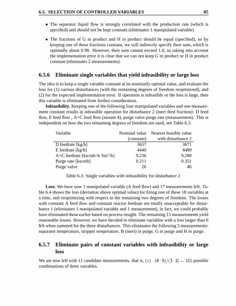
6.5. SELECTION OF CONTROLLED VARIABLES 85y The separatorliquid flow is strongly correlatedwith the productionrate (which isspecified)andshouldnotbekeptconstant(eliminates1 manipulatedvariable)y The fractionsof G in productand H in productshouldbe equal(specified),so bykeepingoneof thesefractionsconstant,we will indirectly specifytheir sum,which isoptimally about0.98. However, their sumcannotexceed1.0, so taking into accounttheimplementationerror it is clearthatwe cannot keepG in productor H in productconstant(eliminates2 measurements).
6.5.6 Eliminate singlevariables that yield infeasibility or largeloss
Theideais to keepasinglevariableconstantat its nominallyoptimalvalue,andevaluatethelossfor (1) variousdisturbances(with theremainingdegreesof freedomreoptimized),and(2) for theexpectedimplementationerror. If operationis infeasibleor thelossis large,thenthis variableis eliminatedfrom furtherconsideration.
Infeasibility . Keepingoneof thefollowing four manipulatedvariablesandonemeasure-mentconstantresultsin infeasibleoperationfor disturbance2 (inert feedfraction): D feedflow, E feedflow , A+C feedflow (stream4), purgevalvepurgerate(measurement).This isindependenton how thetwo remainingdegreesof freedomareused,seeTable6.3.
Variable Nominalvalue Nearestfeasiblevalue(constant) with disturbance2
D feedrate[kg/h] 3657 3671E feedrate[kg/h] 4440 4489A+C feedrate[kscmh=kSm� /h] 9.236 9.280Purgerate[kscmh] 0.211 0.351Purgevalve 26 46
Table6.3: Singlevariableswith infeasibility for disturbance2
Loss.Wehavenow 1 manipulatedvariable(A feedflow) and17 measurementsleft. Ta-ble 6.4showstheloss(deviation aboveoptimalvalue)for fixing oneof these18 variablesata time, andreoptimizingwith respectto theremainingtwo degreesof freedom.The losseswith constantA feedflow andconstantreactorfeedratearetotally unacceptablefor distur-bance1 (eliminates1 manipulatedvariableand1 measurement),in fact,we couldprobablyhaveeliminatedtheseearlierbasedonprocessinsight.Theremaining15measurementsyieldreasonablelosses.However, wehavedecidedto eliminatevariableswith a losslargerthan6$/hwhensummedfor thethreedisturbances.Thiseliminatesthefollowing 5 measurements:separatortemperature,strippertemperature,B (inert) in purge,G in purgeandH in purge.
6.5.7 Eliminate pairs of constant variables with infeasibility or largeloss
Wearenow left with 11candidatemeasurements.thatis,� {�{?~A{¶þ�~u� �q�(� ÿ�~ *��4 {��b} possible
combinationsof threevariables.
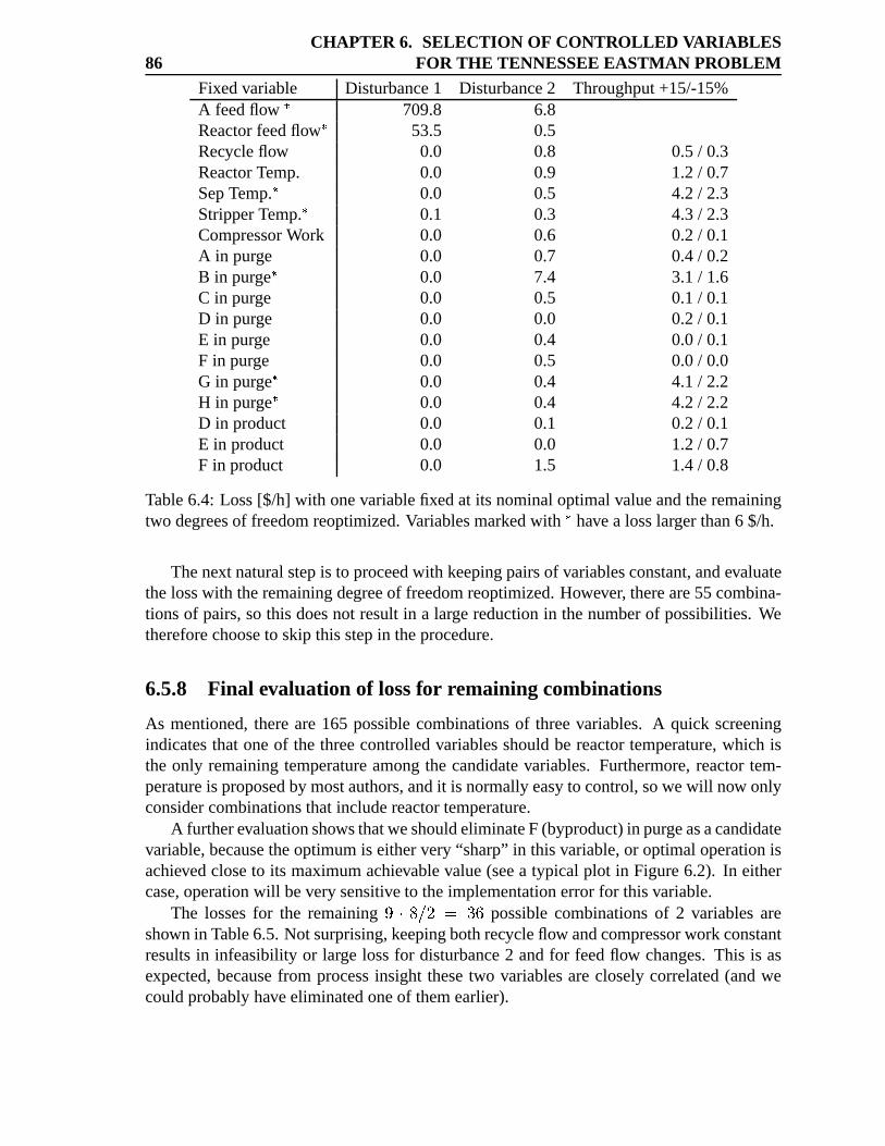
86CHAPTER 6. SELECTION OF CONTROLLED VARIABLES
FOR THE TENNESSEEEASTMAN PROBLEM
Fixedvariable Disturbance1 Disturbance2 Throughput+15/-15%A feedflow � 709.8 6.8Reactorfeedflow � 53.5 0.5Recycle flow 0.0 0.8 0.5/ 0.3ReactorTemp. 0.0 0.9 1.2/ 0.7SepTemp.� 0.0 0.5 4.2/ 2.3StripperTemp.� 0.1 0.3 4.3/ 2.3CompressorWork 0.0 0.6 0.2/ 0.1A in purge 0.0 0.7 0.4/ 0.2B in purge� 0.0 7.4 3.1/ 1.6C in purge 0.0 0.5 0.1/ 0.1D in purge 0.0 0.0 0.2/ 0.1E in purge 0.0 0.4 0.0/ 0.1F in purge 0.0 0.5 0.0/ 0.0G in purge� 0.0 0.4 4.1/ 2.2H in purge� 0.0 0.4 4.2/ 2.2D in product 0.0 0.1 0.2/ 0.1E in product 0.0 0.0 1.2/ 0.7F in product 0.0 1.5 1.4/ 0.8
Table6.4: Loss[$/h] with onevariablefixedat its nominaloptimalvalueandtheremainingtwo degreesof freedomreoptimized.Variablesmarkedwith � havea losslargerthan6 $/h.
Thenext naturalstepis to proceedwith keepingpairsof variablesconstant,andevaluatethelosswith theremainingdegreeof freedomreoptimized.However, thereare55combina-tionsof pairs,so this doesnot resultin a largereductionin thenumberof possibilities.Wethereforechooseto skip this stepin theprocedure.
6.5.8 Final evaluation of lossfor remainingcombinations
As mentioned,thereare165 possiblecombinationsof threevariables. A quick screeningindicatesthatoneof the threecontrolledvariablesshouldbe reactortemperature,which isthe only remainingtemperatureamongthe candidatevariables.Furthermore,reactortem-peratureis proposedby mostauthors,andit is normallyeasyto control,sowewill now onlyconsidercombinationsthatincludereactortemperature.
A furtherevaluationshowsthatweshouldeliminateF (byproduct)in purgeasacandidatevariable,becausetheoptimumis eithervery “sharp” in this variable,or optimaloperationisachievedcloseto its maximumachievablevalue(seea typical plot in Figure6.2). In eithercase,operationwill beverysensitive to theimplementationerrorfor thisvariable.
The lossesfor the remaining �,~�� ��*M ÿ�� possiblecombinationsof 2 variablesareshown in Table6.5.Not surprising,keepingbothrecycleflow andcompressorwork constantresultsin infeasibility or large lossfor disturbance2 andfor feedflow changes.This is asexpected,becausefrom processinsight thesetwo variablesarecloselycorrelated(andwecouldprobablyhaveeliminatedoneof themearlier).
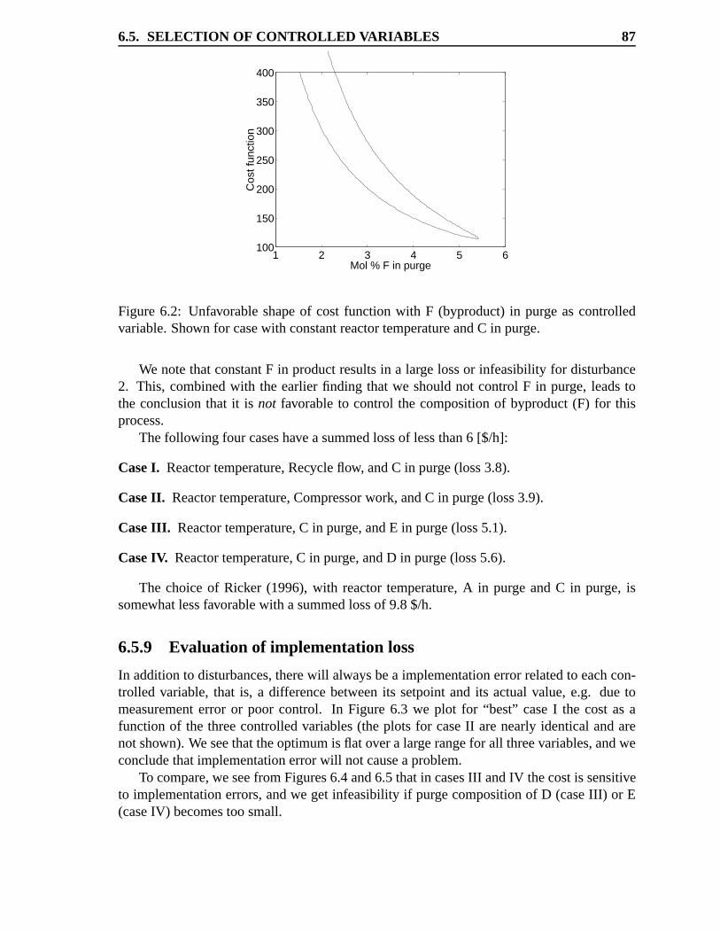
6.5. SELECTION OF CONTROLLED VARIABLES 87
1 2 3 4 5 6100
150
200
250
300
350
400
Mol % F in purgeC
ost f
unct
ion
Figure6.2: Unfavorableshapeof cost function with F (byproduct)in purge ascontrolledvariable.Shown for casewith constantreactortemperatureandC in purge.
We notethatconstantF in productresultsin a large lossor infeasibility for disturbance2. This, combinedwith the earlierfinding that we shouldnot control F in purge, leadstothe conclusionthat it is not favorableto control the compositionof byproduct(F) for thisprocess.
Thefollowing four caseshaveasummedlossof lessthan6 [$/h]:
CaseI. Reactortemperature,Recycleflow, andC in purge(loss3.8).
CaseII. Reactortemperature,Compressorwork, andC in purge(loss3.9).
CaseIII. Reactortemperature,C in purge,andE in purge(loss5.1).
CaseIV. Reactortemperature,C in purge,andD in purge(loss5.6).
The choiceof Ricker (1996),with reactortemperature,A in purge andC in purge, issomewhatlessfavorablewith asummedlossof 9.8$/h.
6.5.9 Evaluation of implementation loss
In additionto disturbances,therewill alwaysbea implementationerrorrelatedto eachcon-trolled variable,that is, a differencebetweenits setpointand its actualvalue,e.g. duetomeasurementerror or poor control. In Figure 6.3 we plot for “best” caseI the cost asafunction of the threecontrolledvariables(the plots for caseII arenearly identicalandarenotshown). Weseethattheoptimumis flat overa largerangefor all threevariables,andweconcludethatimplementationerrorwill not causeaproblem.
To compare,weseefrom Figures6.4and6.5thatin casesIII andIV thecostis sensitiveto implementationerrors,andwe get infeasibility if purgecompositionof D (caseIII) or E(caseIV) becomestoo small.
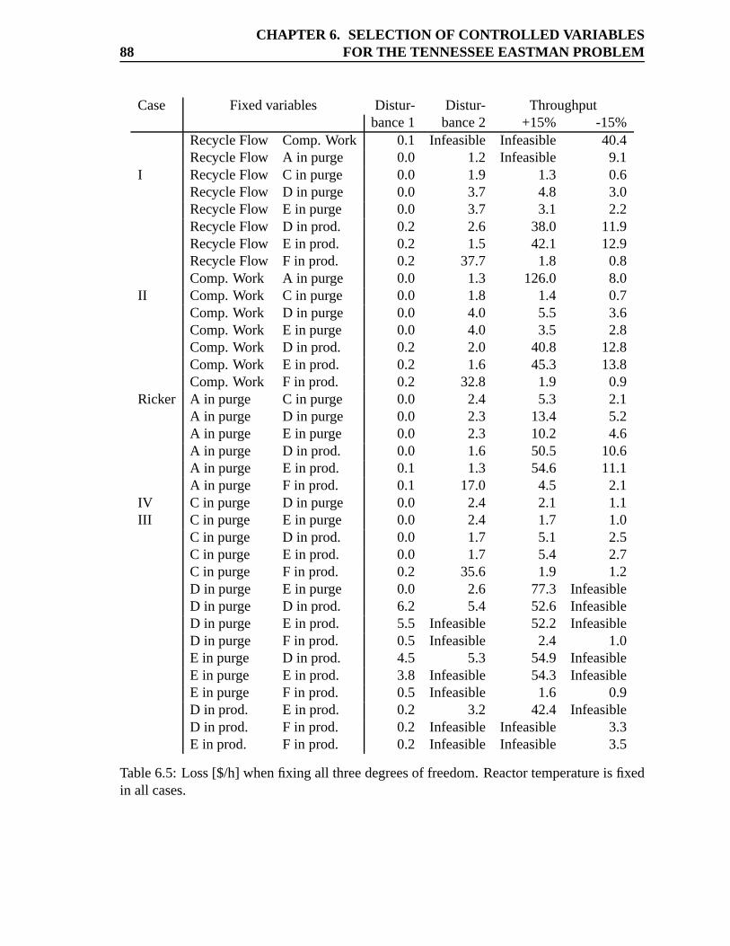
88CHAPTER 6. SELECTION OF CONTROLLED VARIABLES
FOR THE TENNESSEEEASTMAN PROBLEM
Case Fixedvariables Distur- Distur- Throughputbance1 bance2 +15% -15%
RecycleFlow Comp.Work 0.1 Infeasible Infeasible 40.4RecycleFlow A in purge 0.0 1.2 Infeasible 9.1
I RecycleFlow C in purge 0.0 1.9 1.3 0.6RecycleFlow D in purge 0.0 3.7 4.8 3.0RecycleFlow E in purge 0.0 3.7 3.1 2.2RecycleFlow D in prod. 0.2 2.6 38.0 11.9RecycleFlow E in prod. 0.2 1.5 42.1 12.9RecycleFlow F in prod. 0.2 37.7 1.8 0.8Comp.Work A in purge 0.0 1.3 126.0 8.0
II Comp.Work C in purge 0.0 1.8 1.4 0.7Comp.Work D in purge 0.0 4.0 5.5 3.6Comp.Work E in purge 0.0 4.0 3.5 2.8Comp.Work D in prod. 0.2 2.0 40.8 12.8Comp.Work E in prod. 0.2 1.6 45.3 13.8Comp.Work F in prod. 0.2 32.8 1.9 0.9
Ricker A in purge C in purge 0.0 2.4 5.3 2.1A in purge D in purge 0.0 2.3 13.4 5.2A in purge E in purge 0.0 2.3 10.2 4.6A in purge D in prod. 0.0 1.6 50.5 10.6A in purge E in prod. 0.1 1.3 54.6 11.1A in purge F in prod. 0.1 17.0 4.5 2.1
IV C in purge D in purge 0.0 2.4 2.1 1.1III C in purge E in purge 0.0 2.4 1.7 1.0
C in purge D in prod. 0.0 1.7 5.1 2.5C in purge E in prod. 0.0 1.7 5.4 2.7C in purge F in prod. 0.2 35.6 1.9 1.2D in purge E in purge 0.0 2.6 77.3 InfeasibleD in purge D in prod. 6.2 5.4 52.6 InfeasibleD in purge E in prod. 5.5 Infeasible 52.2 InfeasibleD in purge F in prod. 0.5 Infeasible 2.4 1.0E in purge D in prod. 4.5 5.3 54.9 InfeasibleE in purge E in prod. 3.8 Infeasible 54.3 InfeasibleE in purge F in prod. 0.5 Infeasible 1.6 0.9D in prod. E in prod. 0.2 3.2 42.4 InfeasibleD in prod. F in prod. 0.2 Infeasible Infeasible 3.3E in prod. F in prod. 0.2 Infeasible Infeasible 3.5
Table6.5: Loss[$/h] whenfixing all threedegreesof freedom.Reactortemperatureis fixedin all cases.
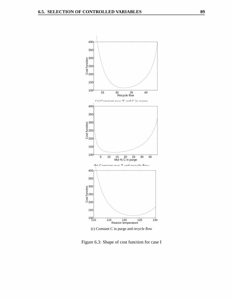
6.5. SELECTION OF CONTROLLED VARIABLES 89
25 30 35 40100
150
200
250
300
350
400
Recycle flow
Cos
t fun
ctio
n
(a)Constantreac.TandC in purge
5 10 15 20 25 30 35100
150
200
250
300
350
400
Mol % C in purge
Cos
t fun
ctio
n
(b) Constantreac.Tandrecycleflow
110 115 120 125 130100
150
200
250
300
350
400
Reactor temperature
Cos
t fun
ctio
n
(c) ConstantC in purgeandrecycleflow
Figure6.3: Shapeof costfunctionfor caseI
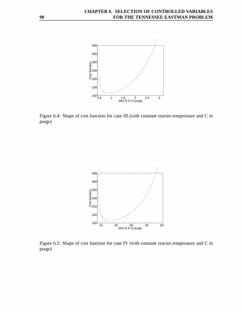
90CHAPTER 6. SELECTION OF CONTROLLED VARIABLES
FOR THE TENNESSEEEASTMAN PROBLEM
0.5 1 1.5 2 2.5 3100
150
200
250
300
350
400
Mol % D in purge
Cos
t fun
ctio
n
Figure6.4: Shapeof costfunction for caseIII (with constantreactortemperatureandC inpurge)
10 20 30 40 50100
150
200
250
300
350
400
Mol % E in purge
Cos
t fun
ctio
n
Figure6.5: Shapeof costfunction for caseIV (with constantreactortemperatureandC inpurge)
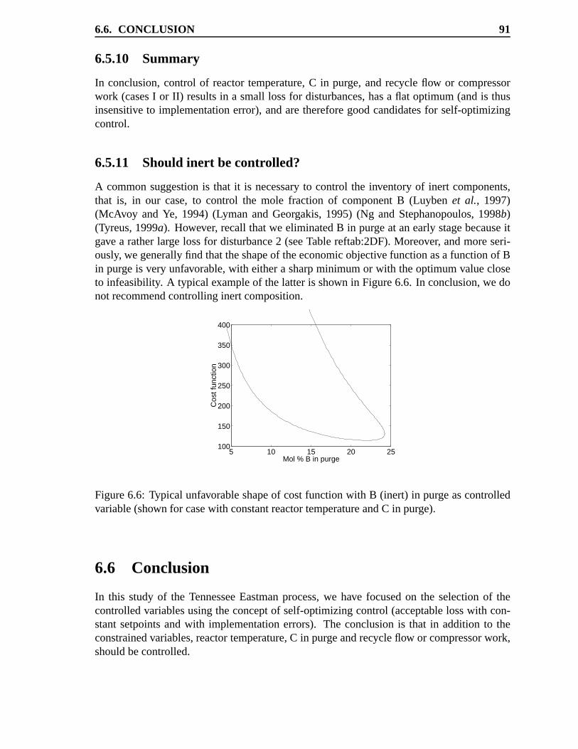
6.6. CONCLUSION 91
6.5.10 Summary
In conclusion,control of reactortemperature,C in purge, andrecycle flow or compressorwork (casesI or II) resultsin a small lossfor disturbances,hasa flat optimum(andis thusinsensitive to implementationerror), andarethereforegoodcandidatesfor self-optimizingcontrol.
6.5.11 Should inert becontrolled?
A commonsuggestionis that it is necessaryto control the inventoryof inert components,that is, in our case,to control the mole fraction of componentB (Luyben et al., 1997)(McAvoy and Ye, 1994) (Lyman and Georgakis,1995) (Ng and Stephanopoulos,1998b)(Tyreus,1999a). However, recall thatwe eliminatedB in purgeat anearlystagebecauseitgave a ratherlarge lossfor disturbance2 (seeTablereftab:2DF).Moreover, andmoreseri-ously, wegenerallyfind thattheshapeof theeconomicobjective functionasa functionof Bin purgeis very unfavorable,with eithera sharpminimumor with theoptimumvaluecloseto infeasibility. A typical exampleof thelatter is shown in Figure6.6. In conclusion,we donot recommendcontrollinginert composition.
5 10 15 20 25100
150
200
250
300
350
400
Mol % B in purge
Cos
t fun
ctio
n
Figure6.6: Typical unfavorableshapeof costfunctionwith B (inert) in purgeascontrolledvariable(shown for casewith constantreactortemperatureandC in purge).
6.6 Conclusion
In this study of the TennesseeEastmanprocess,we have focusedon the selectionof thecontrolledvariablesusingtheconceptof self-optimizingcontrol (acceptablelosswith con-stantsetpointsandwith implementationerrors). The conclusionis that in addition to theconstrainedvariables,reactortemperature,C in purgeandrecycleflow or compressorwork,shouldbecontrolled.
92CHAPTER 6. SELECTION OF CONTROLLED VARIABLES
FOR THE TENNESSEEEASTMAN PROBLEM
Somewhat arbitrarily, we selectedto control reactortemperature.However, sinceourfinal candidateshave goodself-optimizingproperties,it is justifiable. This doesnot meanthatthey arethebestalternative,but “acceptable”is goodenoughhere.
A very commonsuggestion,is that it is necessaryto control theinventoryof inert com-ponents.However, this choicemayleadto seriousoperationalproblemsasdemonstratedbyFigure6.6,andin a morecarefulevaluationwe did not find any favorablecombinationthatincludedtheinert composition.
Wehavepresentedanumberof criteriafor reducingthenumberof alternatives.However,notethatthenumberof alternativeswould havebeenmuchlarger if we alsohadconsideredcombinationsof variables,suchassums,differences,ratiosandsoon. In someapplications,suchasdistillation, theuseof variablecombinationshasprovedto beveryuseful.
All the analysisin this paperis basedon steady-stateeconomics. We have not saidanything on how theproposedcontrol structureshouldbe implemented.This couldbe thesubjectof futurework, andshouldpreferablybebasedon acontrollabilityanalysis.
Chapter 7
Control of an IndustrialHeat Integrated Distillation Column
TrulsLarssonandSigurdSkogestad
Presentedat theAIChE annualmeeting,DallasNovember1999.
Abstract
Heatintegrationof distillationcolumns,wherecondenserandreboilerdutiesarecoupled,is usedto reducetheenergy consumptionusedfor separation.It is well known which variablesto control in normaldistillationcolumns,but for heatintegrateddistillation columnsit is morean openissue. This work will focuson theselectionof controlledvariables.
We usethe conceptof self-optimizingcontrol, (Skogestadet al., 1999), in orderto selectthe controlled
variables.This involvesa searchfor the variableswhich whenkept constantgive operationwith acceptable
economicloss. This providesus with a systematicframework for selectionof controlledvariablesbasedon
steadystateeconomics.
94CHAPTER 7. CONTROL OF AN INDUSTRIAL
HEAT INTEGRATED DISTILLA TION COLUMN
7.1 Intr oduction
Much work hasbeendoneon thecontrolof distillation columns,see(Skogestad,1992)andreferencestherein.Thisshortreview is limited to controlstudiesondoubleeffectdistillationcolumns,andit is far from complete.Therearegoodpapersthathavenotbeenincluded.
TyreusandLuyben(1976)publishedoneof the first papersaddressingcontrol of heatintegrateddistillation columns. Their main conclusionwas to decouplethe two columnsby introducingauxiliary boilersandcondensers.Their conclusionswheresolely basedonsimulations.Lenhoff andMorari (1982)questionedtheir conclusionsincethey did not findsuchaneffect.
Thework by Roffel andFontein(1979)is mostsimilar to our work. They discusssomeaspectsrelatedto constrainedcontrol. Much of their discussionis basedon steadystateeconomicsandactive constraints.Lenhoff andMorari (1982)point out that it is not alwaysoptimalthattheoverheadcompositionsof bothdistillationcolumnsareat their constraints.
Frey et al. (1984)recommendedusingratiosof materialflows asmanipulatedvariables.They usedtherelativegainarrayasacontrollabilitymeasure.
Muchof theabovework usedsimplemodelsthatdid not includeimportanteffects,(likeflow dynamicsor heattransferarea).Grossetal. (1998)presentresultsfor arigorousmodel.They usedcontrollability analysisandnon-linearsimulation,andconcludedthata detailedmodelis neededin orderto captureessentialdetails.
Wewill usetheconceptof self-optimizingcontrol,(Skogestadetal., 1999),for selectionof thecontrolledvariables.This involvesa searchfor thevariablesthatwhenkeptconstantwill giveminimumoperationcost.This providesuswith a systematicframework for selec-tion of controlledvariablesbasedon steadystateeconomics.Finally nonlinearsimulationisusedto confirmthattheself-optimizingcontrolstructurewill work.
7.2 The processand modeling
The plant is shown in Figure 7.1. Methanoland water are feed to the first column thatoperatesat a high pressure.Thebottomflow is feedto thesecondcolumnthatoperatesata lower pressure.Sincethereis ethanolin thefeed,thereis a small sidestreamin the low-pressurecolumnto avoid accumulationof ethanol.Heatis transferredfrom thecondenserinthehigh-pressurecolumnto thereboilerin thelow-pressurecolumn.
This paperis basedon anindustrialcasebut thedesignparametershavebeensomewhatmodified.Themainassumptionsarey Idealequilibriumstages(with fewerstagesthantheactuallynumberof trays).y Thermodynamicsis basedon NRTL-activity coefficientsandidealgas,with parame-
tersfrom (GmehlingandOnken,1977)and(Reidetal., 1987).y Both columnsoperatebelow 10 bar, sothehold-upof vaporis neglected.y Theliquid flows aremodeledby asimplifiedFrancisweir formula.
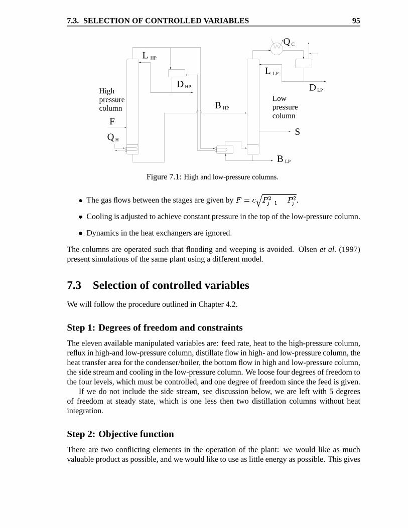
7.3. SELECTION OF CONTROLLED VARIABLES 95
QH
columnpressureHigh
F
Q
L HP
D HP
B HP
C
L LP
D LP
S
B LP
columnpressureLow
Figure7.1: High andlow-pressurecolumns.� Thegasflowsbetweenthestagesaregivenby ���M�A� ����p��)� ���� .� Coolingis adjustedto achieveconstantpressurein thetopof thelow-pressurecolumn.� Dynamicsin theheatexchangersareignored.
The columnsareoperatedsuchthat flooding andweepingis avoided. Olsenet al. (1997)presentsimulationsof thesameplantusingadifferentmodel.
7.3 Selectionof controlled variables
Wewill follow theprocedureoutlinedin Chapter4.2.
Step1: Degreesof fr eedomand constraints
Theelevenavailablemanipulatedvariablesare: feedrate,heatto thehigh-pressurecolumn,refluxin high-andlow-pressurecolumn,distillateflow in high-andlow-pressurecolumn,theheattransferareafor thecondenser/boiler, thebottomflow in highandlow-pressurecolumn,thesidestreamandcoolingin thelow-pressurecolumn.Weloosefour degreesof freedomtothefour levels,whichmustbecontrolled,andonedegreeof freedomsincethefeedis given.
If we do not includethe sidestream,seediscussionbelow, we are left with 5 degreesof freedomat steadystate,which is one lessthen two distillation columnswithout heatintegration.
Step2: Objective function
Thereare two conflicting elementsin the operationof the plant: we would like asmuchvaluableproductaspossible,andwewould liketo useaslittle energy aspossible.Thisgives
96CHAPTER 7. CONTROL OF AN INDUSTRIAL
HEAT INTEGRATED DISTILLA TION COLUMN
theobjective(profit function)to bemaximized:� �M�8�������8 �� �+¡ �)�r¢n£ (7.1)
Where�8���;�¤�| ��¦¥¨§d©5ª-«A¬�B® is thetopproduct(methanol),and ¡ �)�=¥°¯S±M® is theheatloadto thehigh- pressurecolumn,and ¢n£ is therelativecostof energy.
Theconstraintsare:� Thelow-pressurecolumnpressuremustbeabove1 bar.� Thehigh-pressurecolumnpressuremustbebelow 10 bar.� Maximumheattransferareain thecombinedreboiler/condenser.� Purity constrainton topproduct���)�_�"�| �� (molefraction0.99methanol).� Theconstrainton bottompurity ²� �� (molefraction0.99water)is only consideredinrelationto thesidestream.
Step3: Optimization
The five steadystatedegreesof freedomwill be usedfor optimizationandsatisfyingtheconstraints.Wefind thatthefollowing constraintsareat activeat theoptimum:� Thelow-pressurecolumnpressuremustbeabove1 bar.� Maximumheattransferareain thecombinedreboiler/condenser.� Purity constraintson topproduct�8���_�"�| �� (molefraction0.99methanol).
It wasnotedin Roffel andFontein (1979)andLenhoff andMorari (1982) that it wasoptimal for thestreamsof the two distillation columnsto have a differenttop composition.We did not find suchan effect in this work; it wasoptimal with both compositionsat thesamevalues(their constraint).
This resultsin four constraints,andleavesonedegreeof freedomasunconstrained.Fig-ure7.2(a)showsthecombinedmethanolproductionratefrom thetwo columnsasa functionof theheatload.For low heatloadstheproductionincreasessharply. But asthebottomprod-uctgetspurertheincreasein productionratereduces,andapproachestheupperlimit slowly.This figureshows usethat if energy is free(i.e. very low relativecost)thentheprocesswillbeconstrained,eitherby maximumheatload,floodingor pressureconstraints.
SinceFigure7.2(a)hasasharptransitionbetweenasteepincreaseandno increase,it in-dicatesthattheoptimumis nearlyinsensitiveto therelativecostof energy. This is confirmedby Figure7.2(b),which shows the objective asa function of heatload for several relativecosts.With therelativecostof 0.6488mole/MJ,theoptimumheatloadis 66.1MW.
Step4: Disturbances
Themaindisturbanceis feedratevariations,with anassumedrangeof 1200mole/s ³$´�µb¶Feedcompositionhasonly smallvariations,andwill notbeconsidered.
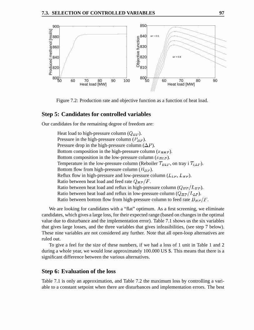
7.3. SELECTION OF CONTROLLED VARIABLES 97
50 60 70 80 90 100800
820
840
860
880
900
Heat load [MW]
Pro
duce
d m
etha
nol [
mol
/s]
50 60 70 80 90800
810
820
830
840
850
Heat load [MW]
Obj
ectiv
e fu
nctio
n
wr = 0.8
wr = 0.5
Figure7.2: Productionrateandobjective functionasa functionof heatload.
Step5: Candidatesfor controlled variables
Our candidatesfor theremainingdegreeof freedomare:
Heatloadto high-pressurecolumn( ¡ �)� ).Pressurein thehigh-pressurecolumn( �N�)� ).Pressuredropin thehigh-pressurecolumn( ·8� ).Bottomcompositionin thehigh-pressurecolumn( ¸�¹.��� ).Bottomcompositionin thelow-pressurecolumn( ¸�¹ �� ).Temperaturein thelow-pressurecolumn(Reboilerº3¹ �� , on tray i º�»½¼ �� ).Bottomflow from high-pressurecolumn( ²<��� ).Refluxflow in high-pressureandlow-pressurecolumn( ¾4 �� , ¾O��� ).Ratiobetweenheatloadandfeedrate ¡ ��� ¬�� .Ratiobetweenheatloadandreflux in high-pressurecolumn( ¡ ����¬�¾O��� ).Ratiobetweenheatloadandreflux in low-pressurecolumn( ¡ ����¬�¾4 �� ).Ratiobetweenbottomflow from high-pressurecolumnto feedrate ²<��� ¬�� .
We arelooking for candidateswith a “flat” optimum.As a first screening,we eliminatecandidates,whichgivesalargeloss,for theirexpectedrange(basedonchangesin theoptimalvaluedueto disturbanceandtheimplementationerror).Table7.1showsusthesix variablesthat giveslarge losses,andthe threevariablesthat givesinfeasibilities,(seestep7 below).Theseninevariablesarenot consideredany further. Notethatall open-loopalternativesareruledout.
To give a feel for thesizeof thesenumbers,if we hada lossof 1 unit in Table1 and2duringawholeyear, wewould loseapproximately100.000US $. Thismeansthatthereis asignificantdifferencebetweenthevariousalternatives.
Step6: Evaluation of the loss
Table7.1 is only anapproximation,andTable7.2 themaximumlossby controllinga vari-ableto a constantsetpointwhentherearedisturbancesandimplementationerrors.Thebest
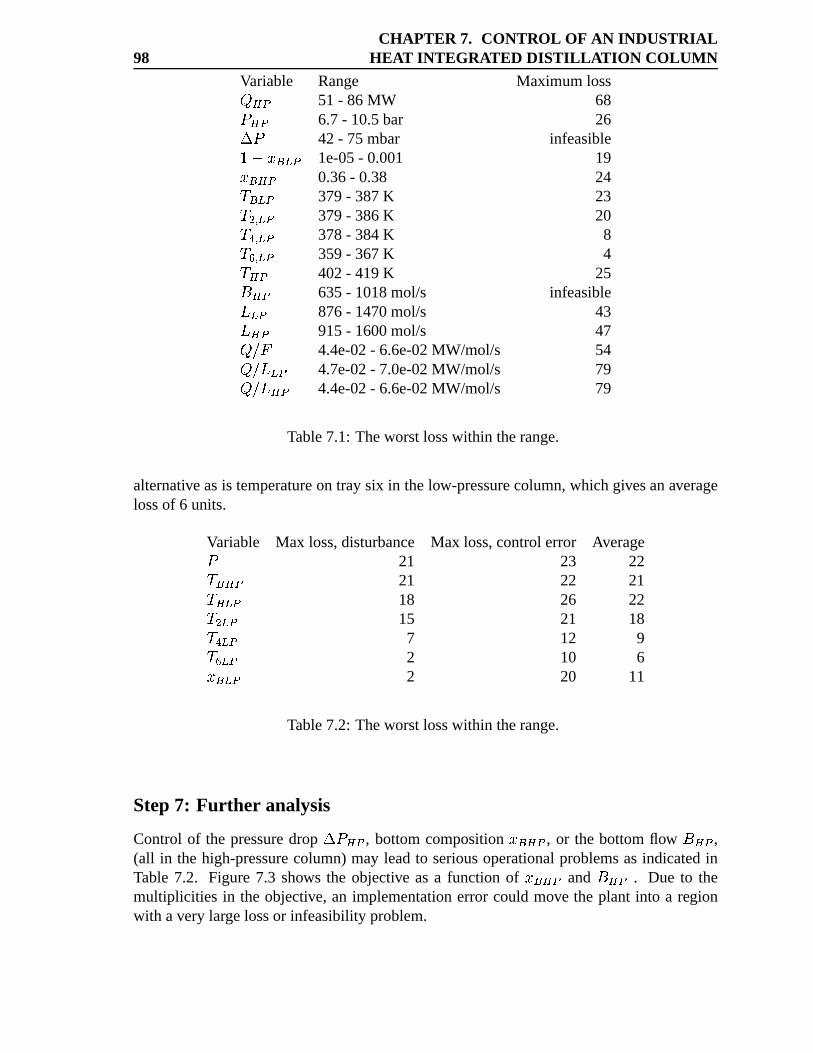
98CHAPTER 7. CONTROL OF AN INDUSTRIAL
HEAT INTEGRATED DISTILLA TION COLUMN
Variable Range Maximumloss¡ ��� 51- 86 MW 68����� 6.7- 10.5bar 26·8� 42- 75 mbar infeasible¿ � ¸�¹ �� 1e-05- 0.001 19¸�¹.��� 0.36- 0.38 24º3¹ �� 379- 387K 23º � ¼ �� 379- 386K 20º�À�¼ �� 378- 384K 8º�ÁQ¼ �� 359- 367K 4º3��� 402- 419K 25²<�)� 635- 1018mol/s infeasible¾4 �� 876- 1470mol/s 43¾O��� 915- 1600mol/s 47¡ ¬�� 4.4e-02- 6.6e-02MW/mol/s 54¡ ¬�¾4 �� 4.7e-02- 7.0e-02MW/mol/s 79¡ ¬�¾O��� 4.4e-02- 6.6e-02MW/mol/s 79
Table7.1: Theworstlosswithin therange.
alternativeasis temperatureon tray six in thelow-pressurecolumn,which givesanaveragelossof 6 units.
Variable Max loss,disturbance Max loss,controlerror Average� 21 23 22º3¹��)� 21 22 21º3¹. �� 18 26 22º � �� 15 21 18º�À& �� 7 12 9º�Á0 �� 2 10 6¸�¹ �� 2 20 11
Table7.2: Theworstlosswithin therange.
Step7: Further analysis
Control of the pressuredrop ·8�N�)� , bottomcomposition�¹.��� , or the bottomflow ²<��� ,(all in the high-pressurecolumn)may leadto seriousoperationalproblemsasindicatedinTable7.2. Figure7.3 shows the objective asa function of ¸�¹.�)� and ²���� . Due to themultiplicities in the objective, an implementationerror could move the plant into a regionwith avery largelossor infeasibilityproblem.
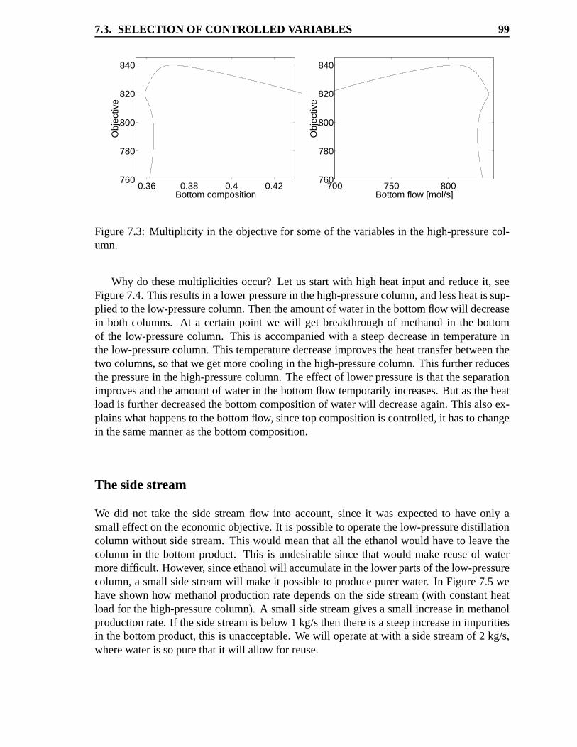
7.3. SELECTION OF CONTROLLED VARIABLES 99
0.36 0.38 0.4 0.42760
780
800
820
840
Bottom composition
Obj
ectiv
e
700 750 800760
780
800
820
840
Bottom flow [mol/s]
Obj
ectiv
e
Figure7.3: Multiplicity in theobjective for someof thevariablesin thehigh-pressurecol-umn.
Why do thesemultiplicities occur? Let usstartwith high heatinput andreduceit, seeFigure7.4.This resultsin a lowerpressurein thehigh-pressurecolumn,andlessheatis sup-plied to thelow-pressurecolumn.Thentheamountof waterin thebottomflow will decreasein both columns. At a certainpoint we will get breakthroughof methanolin the bottomof the low-pressurecolumn. This is accompaniedwith a steepdecreasein temperatureinthelow-pressurecolumn.This temperaturedecreaseimprovestheheattransferbetweenthetwo columns,sothatwegetmorecoolingin thehigh-pressurecolumn.This furtherreducesthepressurein thehigh-pressurecolumn.Theeffect of lowerpressureis thattheseparationimprovesandtheamountof waterin thebottomflow temporarilyincreases.But astheheatloadis furtherdecreasedthebottomcompositionof waterwill decreaseagain.Thisalsoex-plainswhathappensto thebottomflow, sincetopcompositionis controlled,it hasto changein thesamemannerasthebottomcomposition.
The sidestream
We did not take the side streamflow into account,sinceit was expectedto have only asmalleffect on theeconomicobjective. It is possibleto operatethelow-pressuredistillationcolumnwithout sidestream.This would meanthatall theethanolwould have to leave thecolumn in the bottomproduct. This is undesirablesincethat would make reuseof watermoredifficult. However, sinceethanolwill accumulatein thelowerpartsof thelow-pressurecolumn,a smallsidestreamwill make it possibleto producepurerwater. In Figure7.5wehave shown how methanolproductionratedependson the sidestream(with constantheatloadfor thehigh-pressurecolumn). A smallsidestreamgivesa small increasein methanolproductionrate.If thesidestreamis below 1 kg/sthenthereis asteepincreasein impuritiesin thebottomproduct,this is unacceptable.We will operateat with a sidestreamof 2 kg/s,wherewateris sopurethatit will allow for reuse.
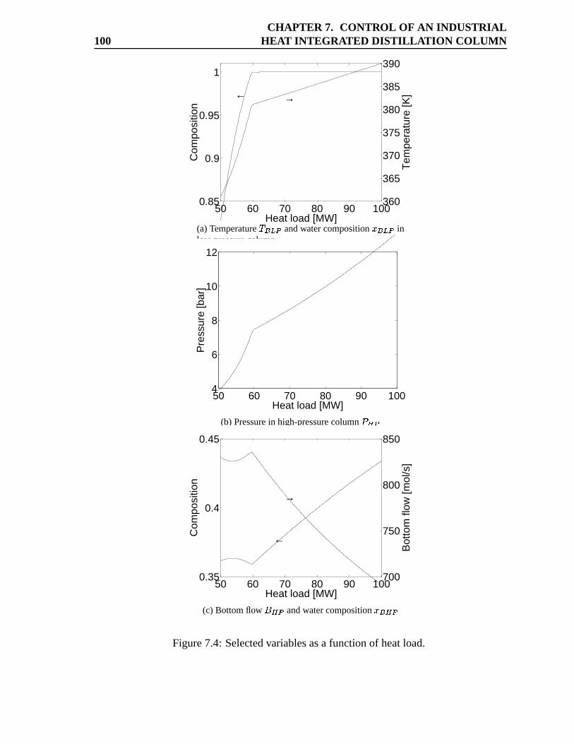
100CHAPTER 7. CONTROL OF AN INDUSTRIAL
HEAT INTEGRATED DISTILLA TION COLUMN
50 60 70 80 90 1000.85
0.9
0.95
1
Com
posi
tion
Heat load [MW]
←
360
365
370
375
380
385
390
Tem
pera
ture
[K]→
(a)TemperatureÂbÃ�ÄAÅ andwatercompositionÆ�Ã�ÄAÅ inlow-pressurecolumn
50 60 70 80 90 1004
6
8
10
12
Heat load [MW]
Pre
ssur
e [b
ar]
(b) Pressurein high-pressurecolumn Ç�È Å
50 60 70 80 90 1000.35
0.4
0.45
Com
posi
tion
Heat load [MW]
←
700
750
800
850
Bot
tom
flow
[mol
/s]
→
(c) Bottomflow ÉNÈ Å andwatercompositionÆ Ã È ÅFigure7.4: Selectedvariablesasa functionof heatload.
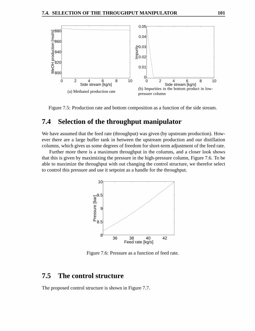
7.4. SELECTION OF THE THROUGHPUT MANIPULA TOR 101
0 2 4 6 8 10
800
820
840
860
880
Side stream [kg/s]
MeO
H p
rodu
ctio
n [m
ol/s
]
(a)Methanolproductionrate
0 2 4 6 8 100
0.01
0.02
0.03
0.04
0.05
Side stream [kg/s]
Impu
rity
(b) Impuritiesin the bottomproductin low-pressurecolumn
Figure7.5: Productionrateandbottomcompositionasa functionof thesidestream.
7.4 Selectionof the thr oughput manipulator
Wehaveassumedthatthefeedrate(throughput)wasgiven(by upstreamproduction).How-ever therearea large buffer tank in betweenthe upstreamproductionandour distillationcolumns,whichgivesussomedegreesof freedomfor short-termadjustmentof thefeedrate.
Furthermorethereis a maximumthroughputin the columns,anda closerlook showsthatthis is givenby maximizingthepressurein thehigh-pressurecolumn,Figure7.6. To beableto maximizethethroughputwith out changingthecontrolstructure,we thereforselectto controlthis pressureanduseit setpointasahandlefor thethroughput.
36 38 40 428
8.5
9
9.5
10
Feed rate [kg/s]
Pre
ssur
e [b
ar]
Figure7.6: Pressureasa functionof feedrate.
7.5 The control structur e
Theproposedcontrolstructureis shown in Figure7.7.
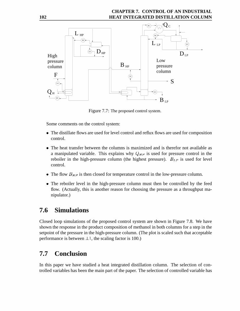
102CHAPTER 7. CONTROL OF AN INDUSTRIAL
HEAT INTEGRATED DISTILLA TION COLUMN
columnpressureHigh
B LP
LC
LC
LC
QH
LC
F
Q
L HP
D HP
B HP
C
L LP
D LP
S
columnpressureLow
PC
TC
PC
XC
XC
Figure7.7: Theproposedcontrolsystem.
Somecommentson thecontrolsystem:� Thedistillateflowsareusedfor level controlandrefluxflowsareusedfor compositioncontrol.� The heattransferbetweenthecolumnsis maximizedandis therefornot availableasa manipulatedvariable. This explainswhy ¡ ��� is usedfor pressurecontrol in thereboiler in the high-pressurecolumn (the highestpressure). ²� �� is usedfor levelcontrol.� Theflow ²<�)� is thenclosedfor temperaturecontrolin thelow-pressurecolumn.� The reboiler level in the high-pressurecolumnmust thenbe controlledby the feedflow. (Actually, this is anotherreasonfor choosingthepressureasa throughputma-nipulator.)
7.6 Simulations
Closedloop simulationsof theproposedcontrol systemareshown in Figure7.8. We haveshown theresponsein theproductcompositionof methanolin bothcolumnsfor astepin thesetpointof thepressurein thehigh-pressurecolumn.(Theplot is scaledsuchthatacceptableperformanceis between³ ¿ , thescalingfactoris 100.)
7.7 Conclusion
In this paperwe have studieda heatintegrateddistillation column. The selectionof con-trolledvariableshasbeenthemainpartof thepaper. Theselectionof controlledvariablehas
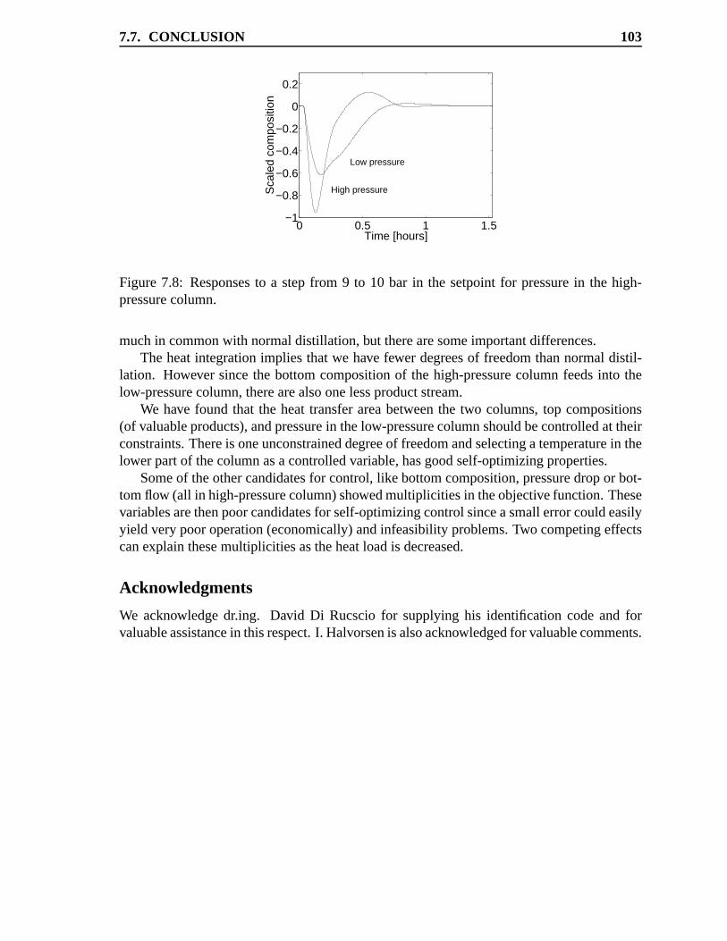
7.7. CONCLUSION 103
0 0.5 1 1.5−1
−0.8
−0.6
−0.4
−0.2
0
0.2
Time [hours]
Sca
led
com
posi
tion
High pressure
Low pressure
Figure7.8: Responsesto a stepfrom 9 to 10 bar in the setpointfor pressurein the high-pressurecolumn.
muchin commonwith normaldistillation,but therearesomeimportantdifferences.Theheatintegrationimplies thatwe have fewer degreesof freedomthannormaldistil-
lation. However sincethe bottomcompositionof the high-pressurecolumnfeedsinto thelow-pressurecolumn,therearealsoonelessproductstream.
We have found that the heattransferareabetweenthe two columns,top compositions(of valuableproducts),andpressurein thelow-pressurecolumnshouldbecontrolledat theirconstraints.Thereis oneunconstraineddegreeof freedomandselectingatemperaturein thelowerpartof thecolumnasacontrolledvariable,hasgoodself-optimizingproperties.
Someof theothercandidatesfor control,likebottomcomposition,pressuredropor bot-tomflow (all in high-pressurecolumn)showedmultiplicities in theobjectivefunction.Thesevariablesarethenpoorcandidatesfor self-optimizingcontrolsinceasmallerrorcouldeasilyyield verypooroperation(economically)andinfeasibilityproblems.Two competingeffectscanexplain thesemultiplicities astheheatloadis decreased.
Acknowledgments
We acknowledgedr.ing. David Di Rucsciofor supplyinghis identificationcodeand forvaluableassistancein thisrespect.I. Halvorsenis alsoacknowledgedfor valuablecomments.

Chapter 8
Polesat the origin inthe Relative Gain Array
TrulsLarssonandSigurdSkogestad
Abstract
Thispapershowshow it is possibleto getpolesat theorigin in therelativegainarray. Thesourceof these
polescanbezerosor polesof theoriginal plant. It is possiblethat integratorswill not cancelout in theRGA,
thereforcaremustbe taken if onewish to follow the approachoutlinedby Woolverton(1980)andMcAvoy
(1998).Thework presentedhereis anargumentfor usingthefrequency dependentRGA.
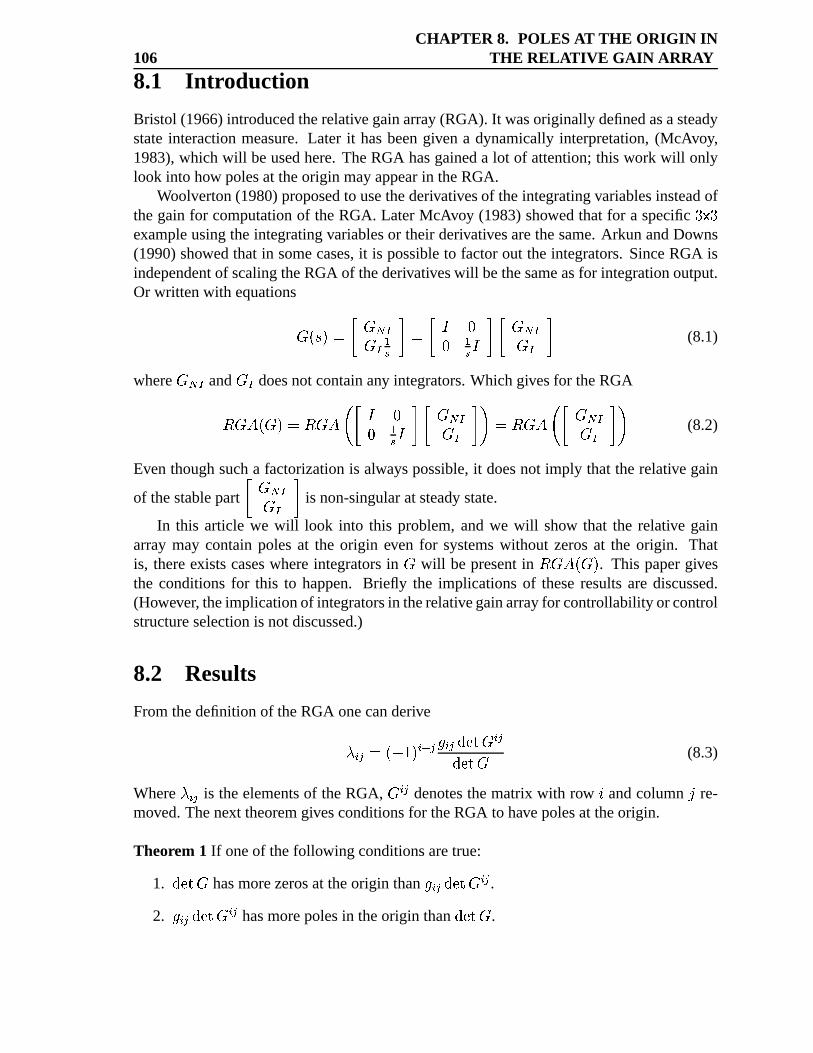
106CHAPTER 8. POLES AT THE ORIGIN IN
THE RELATIVE GAIN ARRAY
8.1 Intr oduction
Bristol (1966)introducedtherelativegainarray(RGA). It wasoriginally definedasasteadystateinteractionmeasure.Later it hasbeengiven a dynamicallyinterpretation,(McAvoy,1983),which will beusedhere.TheRGA hasgaineda lot of attention;this work will onlylook into how polesat theorigin mayappearin theRGA.
Woolverton(1980)proposedto usethederivativesof theintegratingvariablesinsteadofthegain for computationof theRGA. LaterMcAvoy (1983)showedthat for a specific ÊAË�Êexampleusingtheintegratingvariablesor their derivativesarethesame.Arkun andDowns(1990)showedthat in somecases,it is possibleto factorout the integrators.SinceRGA isindependentof scalingtheRGA of thederivativeswill bethesameasfor integrationoutput.Or writtenwith equationsÌ_Í AÎO�ÐÏ Ì;Ñ�ÒÌ;Ò �ÓÕÔ �ÐÏ�Ö µµ �Ó Ö Ô Ï Ì$Ñ)ÒÌ;Ò Ô (8.1)
whereÌ;Ñ�Ò
andÌ�Ò
doesnot containany integrators.Whichgivesfor theRGA× Ì�Ø|Í'Ì ÎO� × Ì�ØÚÙ Ï�Ö µµ �Ó Ö Ô Ï Ì;Ñ�ÒÌ�Ò ÔbÛ � × Ì�ØÚÙ Ï Ì;Ñ�ÒÌ�Ò ÔhÛ (8.2)
Eventhoughsucha factorizationis alwayspossible,it doesnot imply that therelative gain
of thestablepart Ï Ì;Ñ�ÒÌ�Ò Ô is non-singularatsteadystate.
In this article we will look into this problem,andwe will show that the relative gainarray may containpolesat the origin even for systemswithout zerosat the origin. Thatis, thereexists caseswhereintegratorsin
Ìwill be presentin
× Ì;ØvÍ'Ì Î . This papergivesthe conditionsfor this to happen. Briefly the implicationsof theseresultsare discussed.(However, theimplicationof integratorsin therelativegainarrayfor controllabilityorcontrolstructureselectionis notdiscussed.)
8.2 Results
Fromthedefinitionof theRGA onecanderiveÜ » � � Í � ¿ Î »ÞÝ �bß » ��à(átâ Ì » �à(átâ Ì (8.3)
WhereÜ » � is theelementsof theRGA,
Ì » � denotesthematrix with row ã andcolumn ä re-moved.Thenext theoremgivesconditionsfor theRGA to havepolesat theorigin.
Theorem 1 If oneof thefollowing conditionsaretrue:
1. à(áuâ Ì hasmorezerosat theorigin than ß » ��à�átâ Ì » � .2. ß » ��à(áuâ Ì » � hasmorepolesin theorigin than à(áuâ Ì .
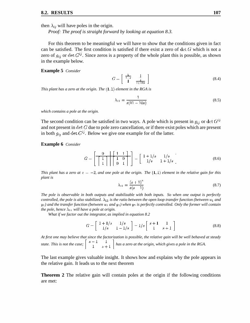
8.2. RESULTS 107
thenÜ » � will havepolesin theorigin.
Proof: Theproof is straight forward by lookingat equation8.3.
For this theoremto bemeaningfulwe will have to show thattheconditionsgivenin factcanbesatisfied.Thefirst conditionis satisfiedif thereexist a zeroof à(áuâ Ì which is not azeroof ß » � or à(áuâ Ì » � . Sincezerosis a propertyof thewholeplantthis is possible,asshownin theexamplebelow.
Example 5 Consider å=æ�çéèè�êìë íí èè-ê�è-î0ë|ï (8.4)
Thisplanthasa zero at theorigin. The ð íuñqíQò elementin theRGAisó è1è æ ô íõ ð íuí�ö,íQ÷ õ ò (8.5)
which containsa poleat theorigin.
Thesecondconditioncanbesatisfiedin two ways.A polewhich is presentin ß » � or à�átâ Ì » �andnotpresentin à(átâ Ì dueto polezerocancellation,or if thereexistpoleswhicharepresentin both ß » � and à(átâ Ì » � . Below wegiveoneexamplefor of thelatter.
Example 6 Consider å=æùøú ÷ û íüí$ýç íí$ï ç íÐ÷÷ í$ïxþÿ æMç í�ödí�� õ í�� õí�� õ í�ödí�� õ ï (8.6)
This plant hasa zero at �æ ô��
, andonepole at the origin. The ð íuñqíQò elementin the relativegain for thisplant is ó è'è æ ð õ ö,í�ò��õ ð õ ö,í�ò (8.7)
The pole is observablein both outputsand stabilizablewith both inputs. So whenone output is perfectlycontrolled, thepoleis alsostabilized.
ó è1èis theratio betweentheopenloop transferfunction(between� è and è ) andthetransferfunction(between� è and è ) when � is perfectlycontrolled. Only theformerwill contain
thepole, henceó è'è
will havea poleat origin.Whatif wefactor out theintegrator, asimpliedin equation8.2å¤æ ç í�ödí�� õ í�� õí�� õ í�ö,í�� õ ï æ í�� õ ç õ ö,í íí õ ö,í ï (8.8)
At firstonemaybelievethat sincethefactorizationis possible, therelativegain will bewell behavedat steady
state. Thisis not thecase;
ç õ ödí íí õ ödí;ï hasa zero at theorigin, which givesa polein theRGA.
Thelastexamplegivesvaluableinsight. It showshow andexplainswhy thepoleappearsintherelativegain. It leadsusto thenext theorem
Theorem 2 The relative gain will containpolesat the origin if the following conditionsaremet:
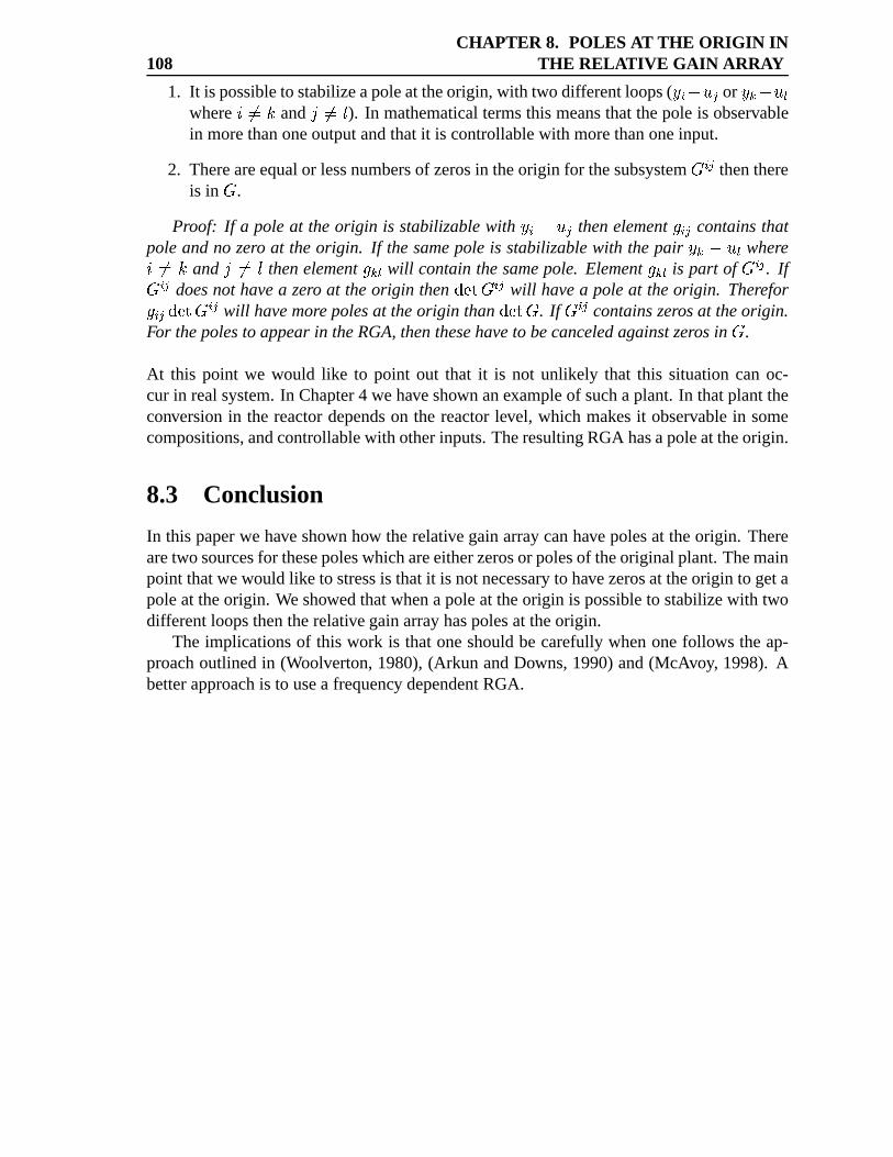
108CHAPTER 8. POLES AT THE ORIGIN IN
THE RELATIVE GAIN ARRAY
1. It is possibleto stabilizeapoleat theorigin, with two differentloops( �» ��� � or � �����where ã����� and ä����ª ). In mathematicaltermsthis meansthatthepole is observablein morethanoneoutputandthatit is controllablewith morethanoneinput.
2. Thereareequalor lessnumbersof zerosin theorigin for thesubsystemÌ » � thenthere
is inÌ
.
Proof: If a poleat theorigin is stabilizablewith �» ��� � thenelementß » � containsthatpoleandno zero at theorigin. If thesamepole is stabilizablewith thepair � ����� whereã����� and ä���ùª thenelementß � will containthesamepole. Elementß � is part of
Ì » � . IfÌ » � doesnot havea zero at theorigin then à(átâ Ì » � will havea poleat theorigin. Thereforß » ��à(áuâ Ì » � will havemorepolesat theorigin than à�átâ Ì . IfÌ » � containszerosat theorigin.
For thepolesto appearin theRGA,thenthesehaveto becanceledagainstzerosinÌ
.
At this point we would like to point out that it is not unlikely that this situationcan oc-cur in realsystem.In Chapter4 wehaveshown anexampleof suchaplant. In thatplanttheconversionin the reactordependson the reactorlevel, which makesit observablein somecompositions,andcontrollablewith otherinputs.TheresultingRGA hasapoleat theorigin.
8.3 Conclusion
In this paperwe have shown how therelativegainarraycanhave polesat theorigin. Therearetwo sourcesfor thesepoleswhichareeitherzerosor polesof theoriginalplant.Themainpoint thatwewould like to stressis thatit is notnecessaryto havezerosat theorigin to getapoleat theorigin. Weshowedthatwhenapoleat theorigin is possibleto stabilizewith twodifferentloopsthentherelativegainarrayhaspolesat theorigin.
The implicationsof this work is thatoneshouldbe carefullywhenonefollows theap-proachoutlinedin (Woolverton,1980),(Arkun andDowns,1990)and(McAvoy, 1998). Abetterapproachis to usea frequency dependentRGA.
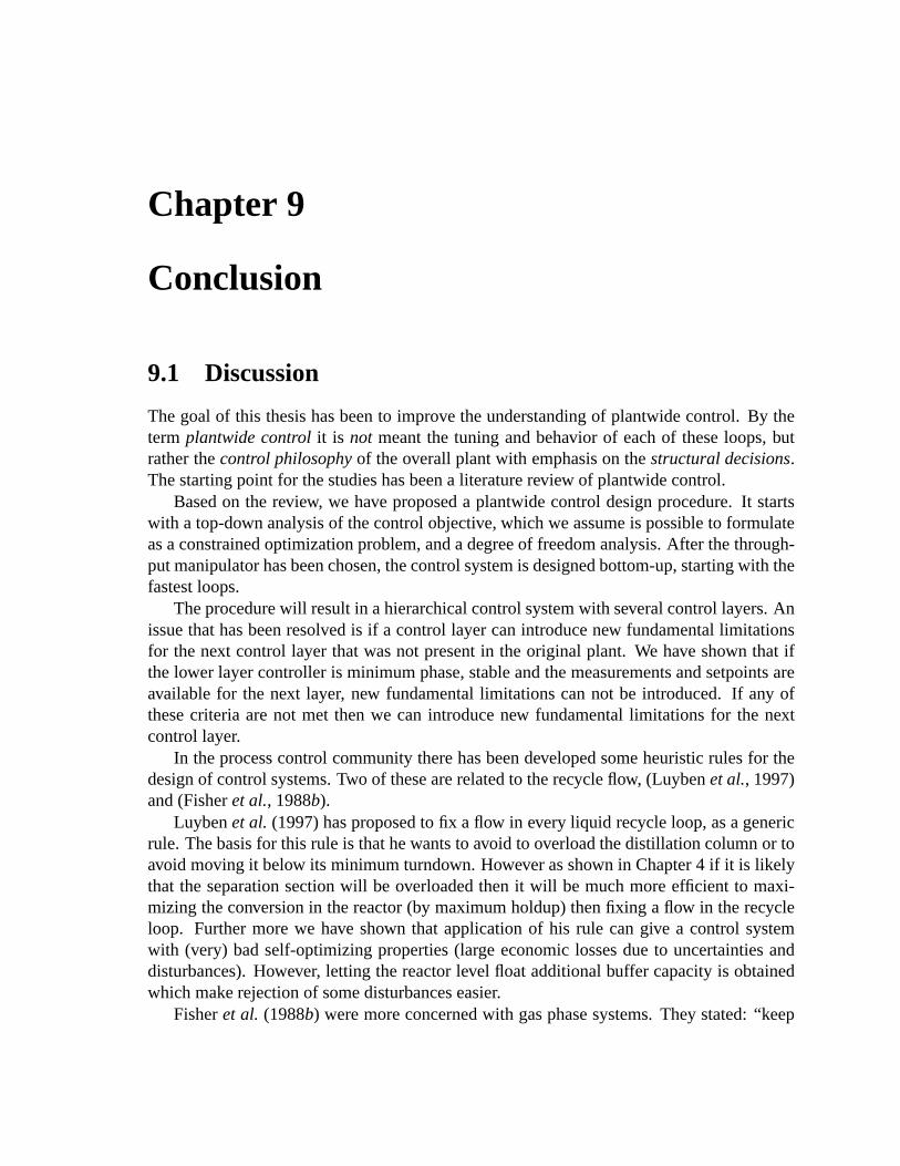
Chapter 9
Conclusion
9.1 Discussion
Thegoalof this thesishasbeento improve theunderstandingof plantwidecontrol. By theterm plantwidecontrol it is not meantthe tuning andbehavior of eachof theseloops,butratherthecontrol philosophyof theoverall plantwith emphasison thestructural decisions.Thestartingpoint for thestudieshasbeena literaturereview of plantwidecontrol.
Basedon the review, we have proposeda plantwidecontrol designprocedure.It startswith a top-down analysisof thecontrolobjective,which we assumeis possibleto formulateasaconstrainedoptimizationproblem,andadegreeof freedomanalysis.After thethrough-putmanipulatorhasbeenchosen,thecontrolsystemis designedbottom-up,startingwith thefastestloops.
Theprocedurewill resultin ahierarchicalcontrolsystemwith severalcontrollayers.Anissuethathasbeenresolvedis if a control layercanintroducenew fundamentallimitationsfor thenext control layer thatwasnot presentin the original plant. We have shown that ifthelower layercontrolleris minimumphase,stableandthemeasurementsandsetpointsareavailablefor the next layer, new fundamentallimitations cannot be introduced. If any ofthesecriteria arenot met thenwe can introducenew fundamentallimitations for the nextcontrollayer.
In theprocesscontrolcommunitytherehasbeendevelopedsomeheuristicrulesfor thedesignof controlsystems.Two of thesearerelatedto therecycleflow, (Luybenetal., 1997)and(Fisheret al., 1988b).
Luybenet al. (1997)hasproposedto fix a flow in every liquid recycle loop,asagenericrule. Thebasisfor this rule is thathewantsto avoid to overloadthedistillationcolumnor toavoid moving it below its minimumturndown. Howeverasshown in Chapter4 if it is likelythat the separationsectionwill be overloadedthenit will be muchmoreefficient to maxi-mizing theconversionin thereactor(by maximumholdup)thenfixing a flow in therecycleloop. Furthermorewe have shown that applicationof his rule cangive a control systemwith (very) badself-optimizingproperties(large economiclossesdueto uncertaintiesanddisturbances).However, letting thereactorlevel float additionalbuffer capacityis obtainedwhich makerejectionof somedisturbanceseasier.
Fisheret al. (1988b) weremoreconcernedwith gasphasesystems.They stated:“keep
110 CHAPTER 9. CONCLUSION
thegasrecycleflow constantatits maximumvalue”,whichis notentirelycorrect.In Chapter5 and 6 we showedthat the recycle flow is an“unconstraineddegreeof freedom”(i.e. theoptimal valueof recycle flow is an unconstrainedvariableandit maximumvaluedoesnotcoincidewith theeconomicoptimum). What they probablymeantwasto keepequipment,like recycle compressor, at their constraints.Which is what they have donein theexamplein (Fisheret al., 1988b). This is confirmedin our casestudies,inputslike control-valvesintherecycle loop, compressor-recycle valve andrecycle compressor(if mountedon separateshaft)whereat their constraintsat theoptimum. Therecycle flow-ratecanalsobeaffected“indirectly” (for exampleby purgeflow), andit actuallyhasgoodself-optimizingproperties.
In a chemicalprocessingplant it is very importantto avoid build-up of inert. Inert willaccumulatewhenits massbalanceis not satisfied.This canhappenif a purge flow is toosmall. This doesnot meantthat the inert compositionshouldbe controlled,with a propersetsof controlledvariablestheinertcompositionwill beself-regulating(e.g.pressurecontrolusingthepurgeflow). Still it is oftenassumedthatcontrol of inert compositionis needed,but aswehaveshown in ourcasestudiesthatit is not true.Inertcompositionis likely to havebadself-optimizingproperties.Often the optimal inert compositionis closeto the highestattainableinert composition,seefigure6.6. Thusa small implementationerrorcanleadtoinfeasibilities.Basedon (Downs,1992),Luybenet al. (1998)recommendsto make a tableover all thecomponentsin orderto checkhow thecontrolsystemwill correctanimbalancein achemicalcomponent.If oneappliestheconceptsof self-optimizingcontrol,suchatablewill notbenecessary.
9.2 Dir ectionsfor futur ework
In this work we have successfullyusedthe conceptof self-optimizingcontrol on severalcasestudies. With a cleardefinition of the control objective anda systematicframeworkfor analysisof the control structurewe have beenable to questionsomeof the heuristicsproposedin processcontrolcommunity. However, thecasestudieshave alsorevealedsomeof theshortcomingsof theprocedure.
In our casestudiesthe numberof measurementand the degreesof freedomto assignthemto wheremodest.But whenthedegreesof freedomthatneedsto beassignedgrows, itquickly becomesimpossibleto analyzeall thealternatives.Goodprocessunderstandingcanhelpat this point,but it mayalsopreventtheengineerfrom seeingthebestsolution.A wayto screenamongthemany alternativesis needed.
Onealternative is to usethemaximizationof theminimumsingularvalue(with properscaling),unfortunatelythelocal informationis probablynot enoughinformation.As canbeseenfrom someof thefiguresin this thesis,it is whenweareatadistancefrom theoptimumthatwegetthelargelosses.Still this approachshouldbefurtherstudied.
A differentalternative could be a mixed-integer-nonlinearprogramming(MINLP) ap-proach.Theproblemformulationanda goodsolver have to befound. Theproblemformu-lation is probablyeasy, but thesolverhasto exploit thestructureof thisproblem.Firstly, thelower boundof a branchis easyto calculatefrom optimization.Secondly, theoptimizationandsteady-statesolver mustbebasedon a continuationmethod.Thelastpoint maybeim-
9.2. DIRECTIONS FOR FUTURE WORK 111
portantsinceinfeasibilitiesarelikely to occur. At leasttoolboxfor automatingmany of thecalculationsis needed.
Very oftentheobjective functionturnedout to have a flat surfacefor severalof thepos-sible controlledvariables. This doesimply that the final choiceshouldbe basedon otherconsiderations.Therearea leasttwo suchvery importantissues,whichhasnotbeenproper-ly addressed:Constraintshandlingandabnormalsituations.
In this thesisall constraintshasbeentreatedequally. However, thereare differences.Someconstraintsarehard if they areviolated it would leadto shutdown of the plant andtherefora largeloss(like theconstraintson reactorpressurein theTennesseeEastmanplan-t). Someconstraintsare “soft”; they may be violateddynamically(like compositionin adistillation column).It is notevengiventhatall theactiveconstraintsaremeasured.For theunmeasuredconstraints,theconceptof partialcontrol,(SkogestadandPostlethwaite,1996),maybesuitable.
For the caseof hardconstraintswith a measurement,a back-off in the setpointfor thiscontrolledvariable is neededto avoid violation of the constraint. The size of the back-off shouldbe assmall aspossible(i.e. ascloseto theoptimumaspossible).However therequiredsizeof theback-off will dependonthecontrolsystemsability to minimizevariationsin thatmeasurement.In futureworks,moreemphasisshouldbegivento thisproblem,it maybe wise to usesomeof the unconstraineddegreesof freedomto achieve tighter control oftheconstraints.A dynamicanalysiswill beneededto addressthis issueproperly. A startingpoint for future work could be alongthe lines of Narraway andPerkins(1993),combinedwith partialcontrolideasof SkogestadandPostlethwaite(1996).
A soft constraintmay not be ascritical, but theremay be caseswherethereis a largeraveragecostfor fluctuationsthenthereis for steadybehavior. Distillation is agoodexample,overpurificationrequiresmoreenergy thanwhatis savedby underpurification.Fewer fluc-tuationsin the compositionwill save energy. Suchbehavior is likely to appearfrequently,dueto the“law” of decreasingoutcome.This dynamiccostis probablymuchmoreimpor-tant than the dynamiccost that is given in (ZhengandMahajannam,1999). This will bechallengingsinceadynamicnon-linearanalysisis needed.
Themostimportanttaskof thecontrolsystemis to avoid ashutdown of theplant.An in-creasein theregularityof theplantwill probablyhaveamuchlargereffectontheeconomicsof the plant thanoptimization. This implies thatgreateremphasisshouldbe placedon thecontrolsystemsability to tackleabnormalsituations.In practicethismeansthatwewill haveto accepta largerlossfor “the usual”disturbance,to beableto handle“rare” disturbance.Itmayevenbeneededto back-off from theoptimumto handlelargeand“rare” disturbances.
As statedmany placesin this thesis,thecontrolsystemis oftendesignedin ahierarchicalmanner, i.e. with abasecontrollayer, asupervisorycontrollayeretc.Thiswastoucheduponin Chapter3 wherewe lookedat thepossibilityto introducenew fundamentallimitationsbyimproperdesignof thelowerlayer. Moreworkshouldbedoneonhow thisstructuringshouldbeandwhich benefitsit is possibleto obtainfrom usinga several layers.Onesuchbenefitof amultilayeredcontrolsystemis believedto robustnessof thehigherlayers.
In practicethe differentcontrol layershave a differentsamplingtime, this implies thatthe higherlayer reactsslower thenthe lower layer. Thusthe higherlayer may not be ableto canceltheeffectsof thelower layer;henceif thesamplingtime is lockedthelower layer

112 CHAPTER 9. CONCLUSION
mayintroducelimitationsfor thehigherlayer. Thiseffectneedsto bestudiedfurther.
Bibliography
Alonso, A.A. and B.E. Ydstie (1996). Processsystems,passivity and the secondlaw ofthermodynamics.Computers& ChemicalEngineering20, S1119–S1124.
Arbel, A., I.H. RinardandR. Shinnar(1996).DynamicsandControlof FluidizedCatalyt-ic Crackers.3. Designingthe Control System:Choiceof ManipulatedandMeasuredVariablesfor PartialControl.Ind. Eng. Chem.Res.35, 2215–2233.
Arkun, Y. andG. Stephanopoulos(1980).Studiesin the synthesisof control structuresforchemicalprocesses:Part iv. designof steady-stateoptimizing control structuresforchemicalprocessunits.AIChEJournal26(6), 975–991.
Arkun, Y. andJ. Downs (1990).A generalmethodto calculateinput-outputgainsandtherelativegainarrayfor integratingprocesses.Computerschem.Engng26, 1101–1110.
Balchen,J.G.andK.I. Mumme (1988).ProcessControl, Structuresand applications. VanNostrandReinhold.
Banerjee,A. and Y. Arkun (1995).Control configurationdesignappliedto the tennesseeeastmanplant-widecontrolproblem.Computers.chem.Engng. 19(4), 453–480.
Bristol,E.H.(1966).Onanew measureof interactionfor multivariableprocesscontrol.IEEETrans.on automaticcontrol pp.133–134.
Buckley, P.S.(1964).Techniquesof Processcontrol. Chap.13. JohnWiley & Sons.
Cao,Y. (1995).ControlStructureSelectionfor ChemicalProcessesUsingInput-OutputCon-trollability Analysis.PhDthesis.Universityof Exeter.
Chang,J.W. andC.C. Yu (1990).The relative gain for non-squaremultivariablesystems.Chem.Eng. Sci.45, 1309–1323.
Douglas,J.M. (1988).ConceptualDesignof ChemicalProcesses. McGraw-Hill.
Downs, J.J.(1992).Distillation control in a plantwidecontrol environment.In: PracticalDistillation Control (W.L. Luyben,Ed.).Chap.20, pp. 413–439.VanNostrandRein-hold.
Downs,J.J.andE.F. Vogel (1993).A plant-wideindustrialprocesscontrol problem.Com-puterschem.Engng. 17, 245–255.
114 BIBLIOGRAPHY
Findeisen,W, F.N. Bailey, M. Brdys,K. Malinowski, P. Tatjewski andA. Wozniak(1980).Control andcoordinationin Hierarchical Systems. JohnWiley & sons.
Fisher, W.R., M.F. DohertyandJ.M. Douglas(1988a). The interfacebetweendesignandcontrol.1, 2 and3.; 1: Processcontrollability, 2: Processoperability3: Selectinga setof controlledvariables..Ind. Eng. Chem.Res.27(4), 597–615.
Fisher, W.R., M.F. DohertyandJ.M. Douglas(1988b). The interfacebetweendesignandcontrol.3: Selectingasetof controlledvariables..Ind. Eng. Chem.Res.27, 611–615.
Foss,C.S.(1973).Critiqueof chemicalprocesscontrol theory. AIChEJournal 19(2), 209–214.
Frey, R.M., M.F. Doherty, J.M. Douglasand M.F. Malone (1984).Controlling thermallylinkeddistillationcolumns.Ind. Eng. Chem.Res.23, 483–490.
Georgakis,C. (1986).On the useof extensive variablesin processdynamicsandcontrol.ChemicalEngineeringScience47(6), 1471–1484.
Gilliland, E.R., L.A. Gould and T.J. Boyle (1964). Dynamic effects of material recycle.PreprintsJACC,Stanford, Calif. pp.140–146.
Gmehling, J. and U. Onken (1977). Vapor-Liquid equilibrium data collection. Vol. 1.DECHEMA.
Grosdidier, P. andM. Morari (1985).Closed-looppropertiesfrom steady-stategaininforma-tion. Ind. Eng. Chem.Fundam.24(2), 221–235.
Gross,F., E. Baumann,A. Geser, D.W.T. RippinandL. Lang(1998).Modelling,simulationandcontrollability analysisof an industrialheat-integrateddistillation process.Com-puters.chem.Engng. 22(1), 223–237.
Haggblom,K.E. andK.V. Waller (1988).Transformationsandconsistency relationsof dis-tillation controlstructures.AIChEJ. 34(10),1634–1648.
Hansen,J.E.(1998).Plantwidedynamicsimulationandcontrolof chemicalprocesses.PhDthesis.DanmarksTekniskeUniversitet.
Havre,K. (1998).Studiesoncontrollabilityanalysisandcontrolstructuredesign.PhDthesis.NTNU Trondheim.Aviablefrom http://www.chembio.ntnu.no/users/skoge/.
Havre, K. andS. Skogestad(1996a). Input/outputselectionandpartial control. PreprintsIFAC ’96, 13th World Congressof IFAC, SanFrancisco,CA, June30-July 5, 1996,VolumeM pp.181–186.
Havre,K. andS.Skogestad(1996b). Selectionof variablesfor regulatorycontrolusingpoledirections.1996AIChEAnnualMeeting, Chicago, Illinois; Paper45f.
BIBLIOGRAPHY 115
Havre, K. andS. Skogestad(1998).Selectionof variablesfor regulatorycontrolusingpolevectors.DYCOPS-5,5th IFAC Symposiumon Dynamicsand Control of ProcessSys-tems,Corfu,Greece, June8-10,1998pp.614–619.
Hestetun,K. (1999).Reguleringav TennesseeEastmanprosessen.Master’s thesis.NTNU.In Norwegian.
Hougen,J. O. and N. F. Brockmeier(1969). Developing ProcessControl Strategies - I:ElevenBasicPrinciples.InstrumentationTechnologypp.45–49.
Hovd, M. andS.Skogestad(1992).Simplefrequency-dependentanttoolsfor controlsystemanalysis,structureselectionanddesign.Automatica.
Hovd, M. andS. Skogestad(1993).Procedurefor RegulatoryControl StructureSelectionwith Applicationto theFCCProcess.AIChEJournal39(12),1938–1953.
Jacobsen,E.W. (1997).Onthedynamicsof integratedplants- non-minimumphasebehavior.To bepublishedin journalof processcontrol.
Jacobsen,E. W. and C. Hong (1998).Zero crossingdue to loop closurein decentralizedcontrolsystems.Presentedat 1998AIChE Annualmeeting,Miami. Paper233e.
Lee, J.H. andM. Morari (1991).Robust measurementsselection.Automatica27(3), 519–527.
Lee,J.H.,P. KesavanandM. Morari (1997).Control structureselectionandrobustcontrolsystemdesignfor a high-puritydistillation column.IEEE Transactionson control sys-temstechnologypp.402–416.
Lee,J.H.,R.D.Braatz,M. Morari andA. Packard(1995).Screeningtoolsfor robustcontrolstructureselection.Automatica31(2), 229–235.
Lee,S. (1990).MethanolSynthesistechnology. CRCPress.
Lenhoff, A.M. andM. Morari (1982).Designof resilientprocessingplants- I. ProcessDe-signUnderConsiderationof DynamicAspects.Chem.Eng. Sci.37(2), 245–258.
Ljung, L. (1987).SystemIdentification- Theoryfor theUser. Prentice-Hall.
Loe, I. (1994).System-struktureri prosessindustrien.Lecturenotes,for a coursegiven atTelemarkCollege.In Norwegian.
Løvik, I, M HillestadandT Hertzberg (1998).Longtermdynamicoptimizationof acatalyticreactorsystem..Computers& ChemicalEngineering22(Supplement),S707–S710.
Luyben,M.L. andB.D. Tyreus(1998).An industrialdesign/controlstudyfor thevinyl ac-etatemonomerprocess.Computers.chem.Engng. 22(7-8),876–877.
116 BIBLIOGRAPHY
Luyben, M.L. andC.A. Floudas(1994).Analyzing the interactionof designandcontrol.2. reactorseparatorrecycle system.Computers & ChemicalEngineering18(10),971–994.
Luyben,M.L. andW.L. Luyben(1995).Designandcontrolof a complex processinvolvingtwo reactionsteps,threedistillationcolumns,andtwo recyclestreams.Ind.Eng. Chem.Res.34(11),3885–3898.
Luyben,M.L., B.D. TyreusandW.L. Luyben(1997).Plantwidecontrol designprocedure.AICHE journal 43(12),3161–3174.
Luyben,W.L. (1975).Steady-stateenergy conservationaspectsof distillationcolumncontrolsystemdesign.Ind. Eng. Chem.Fundam.14(4), 321–325.
Luyben,W.L. (1988).Theconceptof eigenstructurein processcontrol.Ind.Eng. Chem.Res.27(4), 206–208.
Luyben,W.L. (1992).Designandcontrolof recycle processesin ternarysystemswith con-secutive reactions.In: Interactionsbetweenprocessdesignandprocesscontrol. IFACWorkshop.PergamonPress.pp.65–74.
Luyben,W.L. (1993a). Dynamicsandcontrolof recycle systems.1. simpleopen-loopandclosedloopsystems.Ind. Eng. Chem.Res.32(3), 466–475.
Luyben,W.L. (1993b). Dynamicsandcontrolof recycle systems.2. comparisonof alterna-tiveprocessdesigns.Ind. Eng. Chem.Res.32(3), 476–486.
Luyben,W.L. (1993c). DynamicsandControl of Recycle Systems.3. Alternative ProcessDesignsin aTernarySystem. Ind. Eng. Chem.Res.32(6), 1142–1153.
Luyben,W.L. (1994).Snowball effect in reactor/separatorprocesseswith recycle. Ind. Eng.Chem.Res.33(2), 299–305.
Luyben, W.L. (1996). Design and control degreesof freedom. Ind. Eng. Chem. Res.35(7), 2204–2214.
Luyben,W.L., B.D. TyreusandM. Luyben(1998).PlantwideProcessControl. McGraw-Hill.
Lyman,P.R.andC.Georgakis(1995).Plant-widecontrolof theTennesseeEastmanProblem.Computerschem.Engng. 19(3), 321–331.
MacFarlane,A.G.J. andN. Karcanias(1976).Polesandzerosof linear multivariablesys-tems:A survey of thealgebraic,geometricandcomplex-variabletheory. Int. J. Control24(1), 33–74.
Manousiouthakis,V., R. SavageandY. Arkun (1986).Synthesisof decentralizedprocesscontrolstructures.AIChEJournal 32(6), 991–1003.
BIBLIOGRAPHY 117
Marlin, T.E.andA.N. Hrymak(1997).Real-timeoperationsoptimizationof continuouspro-cesses.In: Fifth internationalconferenceon chemicalprocesscontrol (CPC-5,LakeTahoe, Jan.1996). Vol. 93of AIChESymposiumSeries. pp.156–164.
Martens,H. (1989).Multivariatecalibration. Wiley.
McAvoy, T. J. (1983).InteractionAnalysis- PrinciplesandApplications. ISA.
McAvoy, T. J. (1998).A methodologyfor screeninglevel control structuresin plantwidecontrolsystems.Computers.Chem.Engng22(11),1543–1552.
McAvoy, T.J. (1999).Synthesisof plantwidecontrolsystemsusingoptimization.Ind. Eng.Chem.Res.38(8), 2984–2994.
McAvoy, T.J.andN. Ye(1994).Basecontrolfor theTennesseeEastmanproblem.Computerschem.Engng. 18(5), 383–413.
Mizoguchi,A., T.E. Marlin andA.N. Hrymak (1995).Operationsopimizationandcontroldesignfor apetroleumdistillationprocess.CanadianJ. of Chem.Engng. 73, 896–907.
Mizsey, P. and I. Kalmar (1996). Effects of recycle on control of chemicalprocesses.ESCAPE-6,26-29May 1996,Rhodes,Greece;Supplementto Computers & Chemi-cal Engineeringpp.S883–S888.
Morari, M. (1982).Integratedplant control: A solutionat handor a researchtopic for thenext decade?.In: CPC-II. pp.467–495.
Morari, M., G. Stephanopoulosand Y. Arkun (1980).Studiesin the synthesisof controlstructuresfor chemicalprocesses.Part I: Formulationof theproblem.Processdecom-positionandthe classificationof the control task.Analysisof the optimizing controlstructures..AIChEJournal26(2), 220–232.
Narraway, L. andJ. Perkins(1994).Selectionof processcontrol structuresbasedin eco-nomics.Computerschem.Engng18(supplement),S511–S515.
Narraway, L.T. andJ.D.Perkins(1993).Selectionof processcontrolstructurebasedonlineardynamiceconomics.Ind. Eng. Chem.Res.32(11),2681–2692.
Narraway, L.T., J.D. PerkinsandG.W. Barton(1991).Interactionbetweenprocessdesignandprocesscontrol: economicanalysisof processdynamics.J. Proc. Cont. 1, 243–250.
Ng, C. andG. Stephanopoulos(1998a). Plant-widecontrol structuresandstrategies.To bepublishedin ProcessSystemEngineeringSeriesof Academicpress.
Ng, C. and G. Stephanopoulos(1998b). Plant-Wide control structuresand strategies. In:PreprintsDycops-5. IFAC. pp.1–16.
118 BIBLIOGRAPHY
Ogunnaike, B.A. (1995).A contemporaryindustrialperspective on processcontrol theoryandpractice.Dycord+ ’95, 4thIFAC SymposiumonDynamicsandControl of ChemicalReactors,Distillation Columns,andBatchProcesses,Preprints,7-9June1995pp.1–8.
Olsen,I., G.O. EndrestølandT. Sira (1997).A rigorousandefficient distillation columnmodelfor engineeringandtrainingsimulators.Computers.chem.Engng. 21, 193–198.
Olsvik, O.,S.VadaandR. Hansen(1997).StatoilsmetanolanleggpaTjeldbergodden.Kjemipp.42–46.
Papadourakis,A., M.F. DohertyandJ.M. Douglas(1987).Relative gain arrayfor units inplantswith recycle. Ind. Eng. Chem.Res.26(6), 1259–1262.
Ponton,J.W. (1994).Degreesof freedomanalysisin processcontrol.ChemicalEngineeringScience49(13),2089–2095.
Ponton,J.W. andD.M. Laing(1993).A hierarchicalapproachto thedesignof processcontrolsystems.TransIChemE71(PartA), 181–188.
Price,R.M. andC.Georgakis(1993).A plantwideregulatorycontroldesignprocedureusinga tieredframework. Ind. Eng. Chem.Res.32(11),2693–2705.
Price,R.M., P.R. LymanandC. Georgakis(1993).Selectionof throughputmanipulatorsforplant-widecontrolstructures.ECC’93 pp.1060–1066.
Price,R.M., P.R. LymanandC. Georgakis(1994).Throughputmanipulationin plantwidecontrolstructures.Ind. Eng. Chem.Res.33(5), 1197–1207.
Reid, R.C., J.M Prausnitzand B.E Polling (1987). The propertiesof gasesand liquids.McGraw-Hill.
Ricker, N.L. (1995).Optimalsteady-stateoperationof thetennesseeeastmanchallengepro-cess.Computerschem.Engng19(9), 949–959.
Ricker, N.L. (1996).Decentralizedcontrolof theTennesseeEastmanChallengeProcess.J.Proc.Cont.6(4), 205–221.
Rijnsdorp,J.E.(1991).IntegratedProcessControl andautomation. Elsevier.
Rinard,I.H. andJ.J.Downs(1992).Plantwidecontrol:A review andcritique.AIChESpringMeeting1992,New Orleans,paper67f.
Roffel, B. andH.J.Fontein(1979).Constraintcontrolof distillation processes..Chem.Eng.Sci.34, 1007–1018.
Rosenbrock,H.H. (1970).StateSpaceandMultivariableTheory. Nelson.
Scali, C. and C. Cortonesi(1995).Control of the tennesseeeastmanbenchmark:Perfor-manceversusintegrity tradeoff. Proc. of 3rd EuropeanControl Conference, Rome, I-taly, 1995pp.3913–3918.
BIBLIOGRAPHY 119
Seborg, D.E.,T.F. EdgarandD.A. Mellichamp(1995).Processdynamicsandcontrol. Wiley.
Shinnar, R. (1981).Chemicalreactormodelling for purposesof controllerdesign.Cheng.Eng. Commun.9, 73–99.
Shinskey, F.G. (1979).ProcessControl Systems. McGraw-Hill.
Shinskey, F.G. (1988).ProcessControl Systems. McGraw-Hill.
Skogestad,S. (1992).Dynamicsandcontrol of distillation columns- a critical survey. In:PreprintsIFAC-symposiumDYCORD+’92. IFAC. pp.1–25.
Skogestad,S. (2000).Plantwidecontrol: The searchfor the self-optimizingcontrol struc-ture..Acceptedfor publicationsin J. Proc.Control.
Skogestad,S. and E.A. Wolff (1992). Controllability measuresfor disturbancerejection.IFAC Workshop,London,Sept.7-8 1992pp.23–30.Laterprintedin Modeling, Indeti-ficationandControl, 1996,pp167-182.
Skogestad,S. andI. Postlethwaite (1996).Multivariable Feedback Control. JohnWiley &Sons.
Skogestad,S.andM. Hovd (1995).Letterto theeditoronthedecentralizedversusmultivari-ablecontrol.J. Proc.Cont.5(6), 499–400.
Skogestad,S.andM. Morari (1987).Implicationsof largeRGA-elementsoncontrolperfor-mance.Ind. Eng. Chem.Res.26(11),2323–2330.
Skogestad,S. and M. Morari (1988).Understandingthe dynamicbehavior of distillationcolumns.Ind. Eng. Chem.Res.27(10),1848–1862.
Skogestad,S., I.J. Halvorsen,T. LarssonandM.S Govatsmark(1999).Plantwidecontrol:The searchfor the self-optimizingcontrol structure.In: Precedingsof the 13th IFACWorld Congress.
Skrzypek,J.,J.SlooczynskiandS.Ledakowicz (1994).MethanolSynthesis. PolishScientificPublishers.
Stephanopoulos,G. (1982).Synthesisof control systemsfor chemicalplants- a challengefor creativity. Computers& ChemicalEngineering7(4), 331–365.
Tyreus,B.D. (1999a). DominantVariablesfor Partial Control. 2. Application to the Ten-nesseeEastmanChallengeProcess..Ind. Eng. Chem.Res.pp.1444–1455.
Tyreus,B.D. (1999b). Dominantvariablesfor partialcontrol;Part 1 and2. Ind. Eng. Chem.Res.38(4), 1432–1455.
Tyreus, B.D. and W.L. Luyben (1976). Controlling heat integrateddistillation columns.ChemicalEngineeringProgresspp.59–66.
120 BIBLIOGRAPHY
Umeda,T., T. Kuriyamaand A. Ichikawa (1978).A logical structurefor processcontrolsystemsynthesis.Proc. IFAC Congress(Helsinki)1978.
vandeWal, M. andB. deJager(1995).Controlstructuredesign:A survey. In: Proceedingsof theAmericancontrol conference. pp.225–229.
VandenBussche,K. M. andG.F. Froment(1996).A steady-statekineticmodelfor methanolsynthesisandthewatergasshift reactionon a commercial���! #"%$'&( *),+.-�&0/ Catalyst.Journalof Catalysispp.1–10.
Wolff, E. andS.Skogestad(1994).Operabilityof integratedplants.PSE’94, Korea30May-3 June1994pp.63–69.
Wolff, E.A., S. SkogestadandM. Hovd (1992).Controllability of integratedplants.AIChESpringNationalMeetingPaper67a.
Woolverton,P.F. (1980).How to userelative gainanalysisin systemswith integratingvari-ables.InTech pp.63–65.
Wu, K.L. andC.-C.Yu (1996).Reactor/separatorprocesswith recycle-1.candidatecontrolstructurefor operability. Computers.chem.Engng. 20(11),1291–1316.
Wu, K.L. andC.-C.Yu (1997).Operabilityfor processeswith recycles:Interactionbetweendesignandoperationwith applicationto thetennesseeeastmanchallengeprocess.Ind.Eng. Chem.Res.36(6), 2239–2251.
Yi, C.K. andW.L. Luyben(1995).Evaluationof plant-widecontrolstructuresbysteady-statedisturbancesensitivity analysis.Ind. Eng. Chem.Res.34, 2393–2405.
Youla, D.C., J.J.jr. BongiornoandC.N. Lu (1974).Single-loopfeedback-stabilizationoflinearmultivariabledynamicalplants.Automatica10, 159–173.
Zheng,A. andR.V. Mahajannam(1999).A qualitativecontrollability index andits applica-tions.Ind. Eng. Chem.Res.pp.999–1006.
Zheng,A., R.V. MahajannamandJ.M.Douglas(1999).Hierarchicalprocedurefor plantwidecontrolsystemsynthesis.AIChEJournal45, 1255–1265.