NC-4153

Staff: VHPR Problem: 01

Code: I.!] Reprints: Yes

_) EtOLOGI(flL'_ :_ _ mODELLInG

,_ _ ELSEVIER Ecological Modelling II9 (1999) 1-19

-,-I

i.__ An object-oriented forest landscape model and its

,_ _ representation of tree speciesd Hong S. He a.., David J. Mladenoff a, Joel Boeder b0O

" Department of Forest Ecology amt Management, Unieersity of Wisconsin-Madison, 1630 Linden Drive, Madison,WI 53706-1598, USA

_ _ _ _ _ _7"_t,,,_.Ice.,_,_,w_t.g.:_...,io.Soh,tio,,..E,I_.,,.,Vt,V55_35,USA/ Received 24 January 1998; accepted 5 January 1999

v--q 3

Abstract

LANDIS is a forest hmdscape model that simulates the interaction of large landscape processes and forestsuccessional dynamics at tree species level. We discuss how object-oriented design (ODD) approaches such asmodularity, abstraction and encapsulation are integrated into the design of LANDIS. We show that using ODDapproaches, model decisions (olden as model assumptions) can be made at three levels parallel to our understandingof ecological processes. These decisions can be updated with relative efficiency because ODD components are lessinterdependent than those designed with traditional approaches. To further examine object design, we examined howforest species objects, AGELIST (tree age-classes), SPECIE (single species) and SPECIES (species list), are designed,linked and functioned. We also discuss in detail the data structure of AGELIST and show that different data

structures can significantly affect model performance and model application scopes. Following the discussion of forest

species objects, we apply the model to a real forest landscape in northern Wisconsin. We demonstrate the model'scapability of tracking species age cohorts in a spatially explicit manner at each time step. The use of these models at!arge spatial and temporal scales reveals importat:t infarmatkm thct is essential for the management of f(_res_edecosystem. © 1999 Elsevier Science B.V. All rights reserved.

Keywords: Landscape model; LANDIS; Object-oriented design (ODD); Spatially explicit; Tree species; Age class

1. Introduction Pastor, 1993; Turner et al., 1993; Pickett andCadenasso, 1995). These questions must be ad-

Forest ecological research and management are dressed by simulation models that incorporateincreasingly being required to answer questions at spatially explicit dynamics (Mladenoff and Baker,larger, spatial and temporal scales (Mladenoff and 1999). Landscape modelers face the problem that

ecological processes such as seed dispersal,

- *Corresponding author. Tel.: + 1-608-2656321; fax: + 1- seedling establishment, succession, wind and fire608-2629922. disturbance, insect defoliation, forest diseases and

E-mailaddress:hshe@facstaff.wisc.edu (H.S. He) harvesting operate at various spatial and temporal

0304-3800/99/8 - see [}ont matter © 1999 Elsevier Science B.V. All rights reserved.Pti:$0304-3800(99)00041-1

I

2 H.S. ,_feet al. Ecological._lodelh'ng119(1999_1 19

scales. Interactions among these processes are tion). Models using the OOD approach containcomplex and not fully understood. This complex- individual modules that are less interdependent onity has resulted in relatively simple landscape each other, allowing model assumptions to bemodels focusing on a few ecological processes updated with greater flexibility than those de-(Baker and Mladenoff, 1999). To design a land- signed with traditional modeling approaches.

scape model that balances the integration of eco- Applications of OOD to the modeling of bio-logical processes across different spatial and logical systems are increasing (Sequeira et al.,temporal scales, the ability to simulate large areas 1997). Various applications are found in the de-

over long time spans and current computational sign of crop or plant models (Sequeira et al., 1991;capability, is challenging. Acock and Reddy, 1997; Acock and Reynolds,

No model can address issues at all scales. Ex- 1997; Chen and Reynolds, 1997; Lemmon and

plicit and inexplicit assumptions must be made Chuk, 1997; Luo et al., 1997), ecosystem modelingduring the design stage of model development. (Silvert, 1993; Reynolds and Acock, 1997), popu-Decisions are typically made at three levels: (t) lation and forage/energetics dynamics (Moen etwhat ecological processes should be incorporated; al., 1996; Congleton et al. 1997) and species mi-(2) how do these processes interact; and (3) how gration (Maley and Caswell, 1993; Downing andare they represented. These decisions will affect Reed, 1996). Forest landscape modeling is a re-the scopes of the model application as well as the cent endeavor (e.g., Keane et al., 1996; Roberts,model reusability. To be reusable, model updating 1996; Gardner et al., 1999; Mladenoff and He,

is necessary to incorporate increasing understand- 1999; Urban et al., 1999) often assisted by theing of landscape processes. Often, updating a development of spatial information capture andlandscape model involves modifications of built-in processing using remote sensing techniques andmodel assumptions, which can be difficult andtime consuming for models designed with tradi- geographic information system (GIS). The major-tional approaches (Rumbaugh et al., 1991). ity of existing landscape models focus on one

Model development involves a lengthy and in- landscape process, typically fire, assuming thatteractive process of specification, design, verifica- this process overwrites fine-scale dynamics (e.g.,tion, coding, testing, refining, production and Green, 1989; Baker et al., 1991; Turner et al.,maintenance (Carrano, 1995). Approximateiy 60% 1994; Wu and Levin, 1994; Gardner et al., 1996;of development cost lie in the maintenance Li et al., t997). In these models, vegetations are(Varhol, 1992). Therefore, more effective pro- generalized as fire susceptibility classes (Turner etgramming approaches such as object-oriented al., 1994) or as homogeneous stands or patchesprogramming (OOP) are important for optimal with ages represented indirectly by the time sincesoftware reusability and interchangeability. Pro- last distmbancc (Baker et al., 1991; Gustafsougramming tools, however, do not guarantee and Crow, 1994; Gardner et al., 1996; Li et al.,model reusability, as model design plays a major 1997). While disturbance-affected landscape pat-role especially when simulating large complex sys- terns can be successfully investigated over time,terns. Coupled with OOP, object-oriented design the feedbacks and interactions within the dis-(OOD) has emerged as a tool to help build models turbed ecosystems, such as seed dispersal that canthat are maintainable and upgradable. The accelerate ecosystem restoration after distur-essence of OOD includes modularity, abstraction bances (He and Mladenofl; 1998), cannot be sire-and encapsulation fRumbaugh et al., t991; ulated. These feedbacks reveal importantYourdon and Argdar. 1996_. These techniques information when measuring the rates and magni-can be coupled with model decision making pro- tndes of landscape changes (He et al., 1998a).cess at these corresponding levels: tit to specify Vegetation data, with which landscape processeswhat objects to be included tmodularity); (2) to interact, is not incorporated and therefore interac-define how objects interact abstraction); and (3) tions of multiple landscape processes are difficultto decide how objects are represented (encapsula- to examine using these models.

H S, He et _d. Ecologicczl .'_[odelling 119 (1999) 1 19 3

We have developed LANDIS, a spatially ex- • operate on large heterogeneous landscapes atplicit and stochastic landscape model (Mladenoff various spatial resolutions (10-500 m).et al., 1996; Mladenoff and He, 1999). LANDIS • simulate forest succession dynamics at 10-yearsimulates large-scale landscape processes as well time-steps and over long time periods.as fine-scale, species-level vegetation dynamics. • simulate forest landscape change at the individ-The design of LANDIS is based on the OOD ual species level.approach, differing from other forest landscape • simulate wind, fire and harvest disturbances.models. In this paper, we will discuss how OOD • simulate the interaction between succession and

approach is integrated into LANDIS model de- disturbances simultaneously.sign. Specifically, we present the methodology of • simulate seed dispersal in a spatially explicithow species-level vegetation information, such as manner.a list of species present and their age class, in a From the model's perspective, a landscape is aspatially explicit context. We further discuss the grid of equal-sized cells or sites, each havingdata structure of AGELIST and show that differ- unique coordinates. Thus, site (i,j) is the place on

ent data structures can significantly affect model the ground at column i and rowj in the grid (Fig.performance and model application scopes. To 1). The cell size can be varied to accommodatedemonstrate the model capability of tracking studies at different scales. At each site, one orthese species and age-cohort dynamics explicitly multiple species is present, similar to observationsand over long time spans, we analyze the results in the field. Furthermore, existing species mayderived for a real landscape in northern have single or multiple age-cohorts, which areWisconsin. divided into 10-year intervals from age 10 to the

It is impossible to present all components of average longevity of that species (Fig. 1). TheLANDIS in this paper. Further information on species list at one site may differ from those atspecific elements of LANDIS, such as the overall adjacent sites and even if the species list is identi-

cal, the age-classes, may differ. The initial distri-ecological dynamics and model behavior (Mlade- bution of the dominant species can be derivednoff et al., 1996; Mladenoff and He, 1999), fire from a classified satellite image (e.g. Wolter et al.,object (He and Mladenoff, 1999), seed dispersal 1995), or from existing vegetation maps. The as-(He and Mladenoff, 1998) and model parameteri- sociated species and species age-class data can bezation (He et al., 1996; He et al. 1998a,b), can be derived from available GIS and forest survey datafound elsewhere.

te.g. He et al., 1998b). However. use of the modeldoes not have to be strictly subject to theavailability of these detailed data sets, since as-

2. Overall LANDIS design: an OOD perspective sumptlons of species distribution and age can bealways made for a particular area based on the

2.1. Specification of model purpose and scope modeling purposes. For example, randomly dis-tributed, even aged stands are assumed in examin-

The ecological design of LANDIS is similar to mg forest succession dynamics m the MissouriLANDSIM tRoberts. 1996) in successional dy- Ozarks ;Franklin et al.. 1997; Shifley et al.. 1997l.

namics, seed dispersal and fire disturbance, but its Satellite imagery, usually with fine spatial reso-design is object-oriented and it is a raster-based lution such as 30 × 30 m for Landsat TM. can be

model, optimized for greater spatial complexity, re-sampled to a different resolution reflecting theSpecification involves the statement of purpose scale required for a particular research object. It isand model capability in terms of input and out- worth noting that since only the presence or ab-put. The following requirements were identified sence of species age cohorts are tracked, notwhen building LANDIS: individual trees, varying the cell size has less effect

• use satellite imagery as input, which should be on the way that species information is recordedin a format compatible with most GIS than when tracking individuals /Mladenoff andsoftware. He. t999_.

4 H.S. He et aL Eco/ogic*d Modelling II9 (I999) I I9

The environmental condition of each site is scales in LANDIS allows model application to a

defined by ecoregions or landtypes stratifying the wide range of conditions. Assumptions are ap-landscape (Fig. l). Landtype classes are typically plied to the landtype layer in the model design.processed from other GIS layers such as climate Within a landtype unit, homogeneous fire charac-zones, soil maps, or digital elevation models teristics, fuel accumulation rate and individual(DEM), using standard GIS operations (He et al., species response are assumed (Fig. 1). These as-1996). This data layer can also be derived with a sumptions are largely validated by numerousquantitative ecosystem classification that com- studies and expert experiences. For example, firesbines several environmental factors (e.g. Host et are more frequent and have shorter mean returnah, 1996). Landtype coverage is scaleable since interval on xeric landtypes than mesic landtypesproper GIS data layers can be processed accord- (e.g. Kauffman et al., 1988); fuel decompositioning to the research scale. Often however, a re- rate is lower on a xeric landtype than that onsearch scale is confined by the availability of input mesic landtypes (Brown et al., 1982); and speciesdata. The flexibility of using input data at various establishment ability may vary among landtypes.

STRAT,FtEDBV SPEClESAnE F,BEW,NDTHRAWRARVESTSUB-DOMINANT AS t0 YEAR _' ,[, ,_ at site(i,])SPECIES AGECOHORTS

,_ _ DISTURBANCE --SPECIES LIST AND AGE COHORTSspeclesl: age 1, age 2,.., longevity1

SATELLITE J, species: age 1, age 2, ..., longevity 2IMAGERYOR duC mn i

speclesr.: age 1, age 2, ..., tongevi_'mVEGETATION

MAP _ -- SPECIESlife historyattributeestablishmentcapability

I' speciesfire susceptibilityCANBE species.wind susceptibility

RE-SAMPLEDTO VARIOUS sial, j) towj -- FIRE DISTURBANCE

SPATIAL the time since lasttire

PROCESSEDFROM RESOLUTIONS fuel levelOTHERGIBLAYERS fire probabilitySUCHASSOIL,DEM, fireseverity

ANDCLIMATE.

CANBESCALEABLE -- WINDTHRAW DISTURBANCETO REFLECTi - the umesince lastwindVARIOUSSCALES FUEL i winclthrawprobability

ACCUMULATION CONCEPTUALGRID win_hraw severity

t -- HARVEST[ managementunit

ECOREGtON SUCCESSION, stand IDOR LANDTYPE SEED DISPERSAL lasttreatment

neighboringstand IDsa,,

EFFECTIVESPECIES MEANFIRE SHADETOLERANCE ANDMAXIMUM

ESTABLISHMENT SIZEAND FIRETOLERANCE SEEDINGDIFFERENCES RETURNINTERVAL LONGEVITY DISTANCES

Fig. 1. Specifications in LANDIS model design. A landscape can be conceptualized as a grid of equal-sized individual cells or sites.

e.g, site (i,j) and is stratified into environmentally homogeneous units as landtypes or ecoregions. Each site (i,j on a certain

[andtype. records a unique species list and age cohorts of species. These species data change wa establishment, succession and seed

dispersal and interact with disturbances. The initial species and age cohort informauon can be derived from a species-level satelliteclassification or other existing vegetauon map.

H S. He et al. Et'o ogical ,_[oddling 119 (I999) I I9 5

In other words, certain laudtypes favor certain decomposition dynamics of the particular land-species over others. Therefore when a seed travels type. Interactions between these two disturbancesfrom site (re,n) to site (x,y), it may or may not can be interesting and complex. Generally,establish there depending on its establishment windthrow becomes more important on landtypesability on the landtype where site (x, y) is lo- with long-lived species and where fire frequency iscared, low. Mean disturbance return intervals and mean

Succession at each site is a competitive process disturbance sizes can be derived from informationdriven by species life history attributes. In con- in the literature on the region of interest (e.g.trast to most gap models which track each indi- Heinselman, 1973, 1981; Canham and Loucks,vidual tree, succession (if included) is simplified in 1984; Frelich and Lorimer, 1991).landscape models (e.g. Mladenoff et al., 1996;Roberts, 1996). Species competitive ability is 2.2. Modularity and abstractionmainly the combination of shade tolerance,longevity, vegetative reproduction capability, The essence of OOD is modularity, to where aseeding capability and landtype suitability (Fig. complex problem is broken into multiple small1). Seed dispersal is directly related to species and simple modules. In our case, the modules areeffective and maximum seeding distances and it is the various ecological processes identified duringalso strongly affected by the existing seed source, model specification. Ecological processes differ inwhich in turnt can be highly altered by human terms of the spatial and temporal scales at whichand natural disturbances (He and Mladenoff, they operate. For example, species life history1998). Spatially explicit seed dispersal needs to be attributes are static, independent of both spatialdesigned to reflect this reality (Mladenoff et al., and temporal scales. Landtype, which may vary1996). with spatial scales, is independent of temporal

Simulation of disturbance is combined with scale. Processes such as succession are constantlysimulating succession. Any simulated disturbance occurring on every site as long as a species exists.is a result of spatially explicit interaction of envi- Seeding or seed dispersal also occurs constantlyronmental variables, vegetation information and but operates at spatial extents larger than a singlethe nature of disturbance itself. Fire and site. Other ecological processes such as fire, windwindthrow disturbances may occur at various 1o- and harvest occur at landscape scales with strong

cations on the landscape, with each event varying temporal variations. Therefore in abstraction,in time and form of occurrence. Neither the time ecological processes can be described as moduleswhen a disturbance occurs nor the pattern and or objects from the spatially and temporally con-shape of the disturbance is deterministic. They stant to the spatially and temporally explicit (Fig.appea_ to be stochastic for a single site. Over a 2). For spatially explicit landscape modeling, it isheterogeneous landscape however, they are not also necessary to identify the geographic objectspurely stochastic events since some landtypes and where ecological processes occur. SITES andsites may be more prone to disturbance than SITE occur as geographical objects on the land-others, scape where various processes interact. SITES

Fire is a bottom-up disturbance, since fires of divide the entire landscape into rows andincreasing severity affect younger age-classes first, columns comprising singular SITEs (Fig. 1).Fire severity is determined by fuel availability, SITES and SITE link spatially and/or temporallywhich is based on time since the last fire and constant modules with spatially and/or tempo-landtype characteristics that influence fuel pro- rally explicit modules (Fig. 2). Each SITE con-duction and decomposition (He and Mladenoff. tains unique information regarding SPECIES and1999). Windthrow is a top-down disturbance and their AGELISTs. which change via SUCCES-the probability increases with tree age and s_ze. SION through time. Information on LAND-The time since a windthrow event can also influ- TYPE. a spatially explicit and temporallyence the potential fire severity class, depending on constant object, can be referenced from each

6 H.S. He et al. EcologicalModelling119(1999)1 19

Fig. 2. LANDIS Modules.The modulescorrespondto the realworldobjectsfromspatiallyand temporallyconstantto spatiallyandtemporallyexplicit.

SITE. SEEDING, WIND, FIRE and HARVEST, 2.3. Encapsulationall spatially and temporally explicit processes, re-quire spatial extents larger than a single SITE and If modularity and abstraction involve high-leveloperate on SITES, Interactions among FIRE. model decisions related to multiple objects, encap-WIND and HARVEST exist stnce windthrows sulations involves low-level decisions that are ob-

can potentially increase fire severity by adding jeer-specific, linking the high level model designfuels load due to blown-down trees and harvest- (modularity and abstraction) to low level imple-mg also affects fire probability and severity by menting, Encapsulation emphasizes the design ofchanging the fuel regimes (Fig. 2). each object, including its internal (private member

Modularity and abstraction are often closely funt:tions/and external (public member function)tied with model assumptions made during the _nterfaces and data structure [data member).design stage based on the purpose of the model.For example, wind, fire. or other disturbances 2.3.1. Interfacecan be integrated into one module. DISTUR- An internal interface contains the internal func-BANCE. or separated into individual modules, tions or operattons that can be only initiatedNew spatially and temporally explicit modules within an object (e.g. Fig. 41. The idea of ansuch as forest DISEASE or INSECT defolia- internal interface originated with the informationtion can be added to the model LANDTYPE hiding approach (Pohl. 19931. The basic approachcan be further stratified into LANDFORM and is that certain operations on the internal dataSOIL In all cases, assumptions built into the structure should only be accessed from the objectmodel define the scope of model application when inheritance and polymorphism are revolvedto disturbance. With OOD approaches these up- m the model design (Carrano, 1995l. The tech-dates have little impact on the overall model tuque ts widely used in commercial software sincestructure, accessibility involves highly sensitive security is-

H.S. He et al. Ecoiogu'al Modelling 119 ¢I999) 1-I9 7

sues (Booch, 1994). Internal functions can be 3. Example of object design: forest species objectsomitted while external interfaces communicate

with other objects and operate on the internal In the following sections, we further discuss thedata members. It is generally true for ecological design of forest species objects, AGELIST, SPE-modeling that little effort is made on information CIE and SPECIES, particularly their data struc-

hiding (e.g. Sequeira et al., 1997). For LANDIS tures, linkages and functions.objects, several internal operations are imple-mented, including the ability to 'read', 'write', 3.1. Age class (AGELIST object)'copy' and 'dump' the internal data structure (e.g.Fig. 4). These are designed for input, output and AGELIST is an object designed to store speciesdebugging purposes. These operations are stan- age class information. It is generic and once de-dard for all LANDIS objects, signed, it can be populated with any forest spe-

The external interface of an object includes a cies. AGELISTs are objects processing the

set of public operations defined for the object (e.g. greatest computer memory requirements in LAN-Fig. 4). It defines how a given object communi- DIS model. Factors to consider when choosing acares with other objects. In most cases model data structure include the efficiency (of commonupdates involve re-defining, refining, replacing, operations on the data), the memory overheador adding new functions to the external interface and implementation complexity. To illustrateof certain objects. Under an OOD approach, these, we use an example to compare several

typical data structures that can be employed inchanging an interface does not necessarily affect

other object components. For example, changes AGELIST. Assuming that we are simulating amade to the external interface of an object landscape with only ten species, species and their

age cohort data for a particular SITE are listed inmay have no impact on the internal interface Table 1.and the data structure of that object. Thismakes the model updates and software reuse eas-

3.1.I. Array based data structureier than those designed with the traditional ap- Arrays are the most popular data structures. Aproaches, single species can be represented as an array with

s_ze corresponding to the longevity of the species.2.3.2. Data structure To record all the possible age cohorts of the

The selection of data structures for the internal above species, ten arrays with various sizes areimplementation of an object is an important needed: Balsam-fir E15], Aspen [9], Sugar-maple

process in model design. Data structures for [30], Yellow-birch [20], Paper-birch [12], White-different objects can vary significantly, such as pine [40], Red-pine [25], Red-oak [25], White-those for fire (He and Mladenoff, 1999) and cedar [25] and hemlock [45]. Arrays are designedfor species age cohorts, each designed to effec- for efficient access. Some common succession op-tively accommodate the corresponding func- erations such as insertion (insert an age cohort,tions. The data structure implemented can sub- e.g, germination or new seed establishment) and

stantially affect the performance in terms of deletion _remove an age cohort, e.g. species death)running time of an application or simulation are very efficient. Retrieval (e.g. locate certain age

size limit. The rationale for employing a particu- cohort_ is very efficient too. These operations arelar data structure is often not fully explained in used by SUCCESSION and HARVEST for re-descriptions of models that simulate biological moval of certain species which have reached their

systems (e.g. Chen and Reynolds, 1997: Sequeira longevity, or for planting certain species at age 10.et al., 1997). Since increasing model updates m- However. existence querying (e.g. search age co-volve the replacement of old data structures, a hort to determine if a species exists) is inefficientcomparison of various alternatives becomes im- with arrays. In the wirst case. every data memberportant, has to be visited before the program knows that

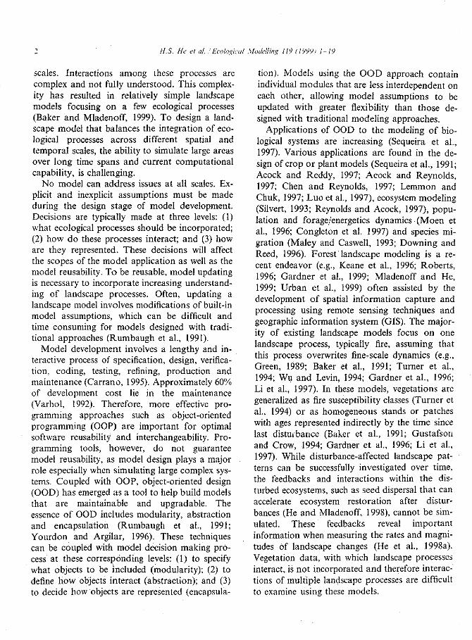
8 H.S. He eta] EcologicalModetloTg1I9 (1999) 1-19

Table 1Typicalarray representationof speciesage cohorts

Species Age-cohorts(years) Longevity(years) Arrays

Balsamfir 10,80 150 Balsam-for[1-15]Quaking aspen not present 90 Aspen[1-91Sugar maple 40, 90, 190,270, 290 300 Sugar-maple[1-30]Yellowbirch 200 300 Yellow-birch[I-30]Paper birch not present 120 Paper-birch[1-12]White pine 250 400 White-pine[1-40]Red pine not present 250 Red-pine[l-25]Red oak not present 250 Red-oak [1-25]Whitecedar not present 250 White-cedar[1-25]Hemlock 10,20, I00, 150, 200 450 Hemlock[I-45]

aspen is not present at the above sample SITE. tion is contained in an array, say, BitArray [10]This may suggest a significant drawback in speed, (Table 2).

since existence querying is one of the most corn- Since each digit represents a bit, on a 32-bitmon and time-consuming operations in machine, 64 digits can represent species longevity

AGELIST. up to 640 years, which satisfies all common treeIf age presence or absence is represented as an species found in the Eastern US (Burns and Han-

integer (each array element holding one integer), kala, 1990). For the example SITE, the bit-wise

there is a total of 256 integers needed for the representation of an array of size 10 takes only 40SITE, the sum of all array elements. On a 32-bit bytes to represent all age cohorts in the SITEcomputer, with each integer taking 4 bytes of (Table 2). For a landscape containing 300 x 300memory, this equals 1024 bytes (Table 1). Since SITEs, total memory required for storing speciesthe same set of arrays is needed for every single age information is less than 4 MB. If simulatingSITE, assuming the simulated landscape contains300 (rows)× 300 (columns) SITEs, the total Table 2amount of memory used for species information is Bit-wisearray representation of species age-cohorts300 x 300 x 1024 bytes, or about 90 MB. For asimulation of the same landscape containing 30 Species Age-cohorts Array

species assuming the longevity of average spectesis 150 years, the minimum memory required for Balsamfir 0100000010000000 Bit-array [1]Aspen 00000000_0 Bit-array [2]species information alone is about 154 MB. Even Sugar maple O00010000100000000010Bit-array [3]if we replace the integer representation with char- 0000001010acters [one character requtres 2 bytes), reducing Yellowbirch 000000000000000000001 Bxt-array[4]the memory requirement to about 77 MB. an 0000000000array-based implementation is impractical as Paper birch 000000000000 Bit-array[5]Whitepine 000000000000000000000 Bit-array[6]demonstrated. If employed it can significantly 00001000000000000oo0limit model application to small areas Red pine 00000000O000000000000Bit-array[7]

00000Red _ak 0O0000000000000000000 Bit-array[8]

3.1.2. Bit-wise based data structure ooooo

In bit-wise representation, the species age list is Whitecedar 000000O00000000000000Bit-array [9j

represented as an array of binary data with each oooooHemlock 01lgO0000010000010000 Bit-arra_[10]element containing 0 or 1: O. denotes the species OLOOOOOOOOOOOOOOOOOOOage cohort absent: and 1, denotes present. Thus 0000for the example SITE, species age cohort informa-

It.S He et a: Ecok_ica! ._fode::i_lg 119 (1999) I- 19 9

tSug,rmo 'o i :70 .-

r W t°pin°

b)

...) ...)

Speciesm .,., ...,

Fig. 3. Sorted linkedlist representationfor:(a) speciesage-cohorts;(b) speciesage-cohortsand number of individualtreesor density.

the same landscape with 30 species, total memory are not present) is another inefficiency. It not only

requirement for storing species age cohorts is less wastes memory, but more importantly, can signifi-than 11 MB. Because the bit-wise array is so cantly increase the run time by lengthening the

space efficient, it allows the model to be applied time of existence queries.to large landscapes. Operations such as msertion

at the youngest end and deletion at the oldest end 3.1.3 Sorted linked list

of age cohorts are very efficient in bit-wise opera- A linked list is an abstract data type with each

tion, involving bit shifting. Inserting a particular data element (node) referring to the next elementage cohort (such as planting), or deleting a certain with a pointer. A sorted linked list manages theage cohort in the middle (due to cutting or distur- data in a sequential order (e.g. sorted by value orbance) is no less efficient than insertion or dele- name) One of the advantages of a linked list ts Itstion at the ends. Similar to the array based data reliance upon dynamic allocation of computerstructure, query operation is inefficient. For the memory. Only species and age cohorts present areworst case, every bit has tO be visited to decide stored. The species and their age cohort informa-that aspen does not exist on this SITE. tion from the example SITE can be represented

A significant deficiency that exists for both the with multiple sorted linked lists (Fig. 3a)array and the bit-wise data structure exists with Among these lists, the vertical list constitutes athe fixed 10-year age cohort representation (al- species name list. while horizontal lists comprise

though it wag a specification of design). It is the corresponding age cohorts of the species (Fig.impossible to apply this data structure to simula- 3a_. For this particular SITE. if ages are presentedtions of a time step other than 10 years. Holding as integers, it takes 128 bytes (each pointer takesof empty spaces (e.g. when species or age cohorts 4 bytes). For a landscape containing 300 x 300

i

10 H.S. He et al. Ecological Modelling II9 (I999) I 19

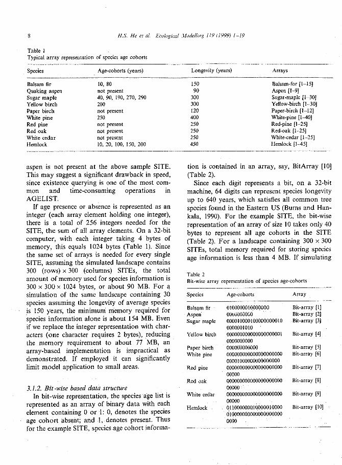
AGELIST A significant advantage of using a linked listdata structure is that the datum of each node canInternal interface External interfacebe any integer. In other words, the model can be

Set youngesttrue ,--- potentially applied to various model time-stepssuch as 1 or 3 years. Also. each node can theoret-

Set oldest null o_ ically have another attribute to keep track either

Shift right _ individual tree species or forest density (Fig. 3b),•"o providing greater potential of model application.

-,_ Set one null oE Disadvantages to using a sorted linked list or2 Set one true -, _ other advanced abstract data types such as vari-t_ ' a ous tree data structures (Carrano. 1995) include-_ query Z that they are more difficult to code than the other

li <c-a ' clear .-J two. Implementation can be much longer than theother two and the resulting programs can be.fie

read _ difficult to debug.

write -] 3.1.4. Interface of AGELISTcopy All external operations defined for AGELIST

dump are species related (Fig. 4). 'Sel youngest true'simulates birth of a species, when a new agecohort is set present at 10 years old. 'Set last null'

Fig, 4. LANDIS obJeCt AGELIST. containing information simulates deatk, when the last age cohort of afor speciesage cohorts on a gwensite (cell). species lS set to null. 'Shift right' simulates

growth, when all age cohorts increase 10 years bySITEs, assuming other SITEs contains the similar moving rightward in the bit-level data structure.species information, total memory required for 'Set one null' simulates removal of a certain spe-storing species age information is only approxi- cles age cohort. 'Set one true' sets a given agemately 12 MB. When expanded to 30 species, the cohort mot necessarily the first), a method usedamount of memory increase• if any, will not be for initialization of age information. 'Clear' simu-significant compared to the other two data struc- lares the removal of an entire age cohort of atures described above. It should be pointed out species. 'Query age cohort' allows other objects tothat with dynamic memory allocation• the actual query for certain age classes, a method frequentlyamount of memory required to represent species requested by SUCCESSION, DISPERSAL•information varies. When the majority of SITEs FIRE. WIND and HARVEST.on the landscape contain most species and multi-

ple ages, memory requirements can be large. 3.2. Single species (SPECIE object_However, [orest landscapes are more often com-

posed of many fewer species and age cohorts than SPECIE is an object designed for a single forestthe theoretical maximums due to compennon, species. Each SPECIE has its own AGELIST andTherefore. the sorted linked list can be a memory- species-specific functions.efficient method for storing species age informa-tion. Common operations of this data structure 3.2.1. Data structure of SPECIEsuch as insertion and deletion are as efficient as a SPECIE inherits data members and interfaces

bit-wise data structure. Additionally, existence from AGELIST. Inheritance. an important fea-querying is much more efficient than the other ture of OOD. is the mechanism by which some

two data structures since only species and age objects are specified as the decedents of others; cohorts present are recorded in lists that are iBooch, t994: Carrano. 1995), In this case. SPE-

, sorted. CIE. a single species object, has whatever data

i

?

ILS, He et ui. Eeo )go _lodelling I19(1999) 1-19 11 _

structure AGELIST implements, whether it is an For example, wind disturbance tends to remove , :.array of integers, a bit-wise array, or horizontal older age cohorts, while fire disturbance tends tosorted linked list. remove younger age cohorts. 'Remove' differs

from 'death' in that it can remove any age cohort

3.2.2. Interface of SPECIE of the species. 'Clear' simulates the removal of the )Operations defined for SPECIE includes the species (entire age cohorts) on the site, which

'name', 'attribute', 'birth', 'death', 'growth', 're- usually accompanies severe fire disturbances or ,move', 'clear' and 'query' (Fig. 5). 'Name' and clear-cut harvest. For example, when SPECIE'attribute' are used to reference species name and interacts with a fire object with severity class ofattributes. 'Birth', 'death', 'growth', 'remove' and four, all age cohorts are cleared if the species' fire'clear' mirror those in AGELIST. 'Birth' simu- tolerance class is of one (He and Mladenoff,

1999).lares a new species seeding in from another site, oron-site species regeneration. The latter usually

3.3. Species list (SPECIES)applies to high shade tolerance species. For somespecies 'birth' simulates vegetative reproduction.'Death' typically simulates species reaching their SPECIES is a list of one or more speciesmaximum longevity. It applies only to the particu- present on a given site. It is implemented with

some generic operations for a list.lar age cohort that reaches species longevity.'Growth' simulates species age-class incrementduring each model iteration. 'Remove' simulates 3.3.1. Data structure of SPECIESthe removal of one or more age cohorts of a SPECIES is an object that maintains a list ofspecies from the site due to various causes. Dis- species present on each SITE. Since it does not

deal with the features of any particular species,turbances, harvest and background mortality can data members of AGELIST are not available to a

all result in removal of certain species age cohorts. SPECIES object. However, since a species list

SPECIE such as the vertical list in the sorted linked listalready exists for any given SITE, there is no need

Internalinterface Externalinterface to define new data structures or allocate separatememory locations to duplicate the same informa-tion. Rather, a pointer to AGELIST is a data _member of SPECIES. This allows a SPECIES

i object to reference an individual SPECIE object. ,_

-- _ Other data members of SPECIES include integers

tracking the current species (ID) and the total.boO

_. number of species on the SITE and a pointer to"_ reference species attributes.

_ -- 3.3.2. Interface of SPECIES-- clear "-' '

._ [ For the most part. the external interface of

_ re-ad_ _],--- _ [ SPECIES includes utility fnnctions to manage thespecies list (Fig. 6I. 'First' sets an internal iterator

___. _ to point at the first species in the list. 'Current'returns a reference to the species currently pointed

----, to by the internal iterator. 'Next' moves the inter-, nal iterator to the next species in the list. 'At-

tributes' returns a reference to the attribute object

Fig. 5. LANDIS object SPECIE, containing information l'or of a given species. 'Number' returns the totalsinglespecieson a givensite (cell). number of species on the SITE. SPECIES is m-

|2 H.S. He et at. Ecologica!Modeth)_g119(1999)1 19

SPECIES dominated by pine (Pinus Strobus, P. resinosa),eastern hemlock (Tsuga canadensis) and sugar

Internalinter[ace Externalinterface maple (Acer saccharum). Yellow birch (Betula _

, _r first _ alleghaniensis), paper birch (B. papyrifera), spruce.... (Picea glauca) and balsam-fir tAbles balsamea)

t ,11 current : ; were also common. Today the region is largely' " next . _._ covered by second and third growth forests fol- i

............. _ -_ lowing extensive logging and fire in the late 19th::3 ( )ll attributes , o

' '" number ;i CO 1992; Mladenoff and Pastor, 1993)....... ... _ t= and early 20th centuries (Pastor and Mladenoff,

k-

t_ O

° d The modelinput map was derived from a clas-

sification of multi-temporal Landsat TM/MSSsatellite imagery, representing spatial distributionsof dominant canopy species or forest types atspecies and genus levels (Wolter et al., 1995).

Fig.6. LANDISobject--SPECIES, containinginformationof Secondary associated species and age-class infor-specieslist on a givensite. marion were derived by integrating the TM clas-

sification with forest inventory plot data (Hansenherited by SITE. The request of query for theet al., 1992), stratified by landtypes (He et al.,

oldest or the youngest species on the SITE is a 1998b). A total of 23 species and 134 unique

common operation. _'_:species-age cohort combinations resulted on theinput map. To reflect the relative growth capabil-

ity of each tree species under the environmental4. Model application conditions of different landtypes, individual spe-

cies establishment coefficients (0-1) were calcu-

To demonstrate the capability of tracking age lated based on species relative performance oncohorts of individual species by the forest species differeut landtypes. These coefficients can be as-objects, we chose a real landscape in northern signed directly by interpreting the available litera-Wisconsin, where simulations have been con- ture or derived from an ecosystem process model _.ducted to examine fire disturbance and succes- (He et at., 1998a)..All life history attributes ofsional dynamics at forest type level (He and species were derived from the literature as re-Mladenoff, 1999). In this paper, we further ana- ported elsewhere (Mladenoff et al., 1996; Mlade-lyze dynamics of forest species at age-classes level, noff and He, 1999). Historical fire data (mean i_illustrating the previous description of forest spe- disturbance size and mean fire return intervals) _

cies objects, were interpreted from empirical studies in theregion (Heinselman. t973 1981: Frelich and

4.1. Study area Lorimer, 1991) Mean fire size was set to 3200 ha.about 3% of the total area. with a maximum fire

The study landscape, comprising nearly 500000 size of 16000 ha. about 15% of the landscape.ha, is located in northwestern Wisconsin (46°9l ° Mean fire return intervals vary among landtypesto 47°92% It is in a transitional zone between the from 200 years on dry and sandy soil. to 500 yearsboreal forest of Canada and the central deciduous well-drained loam), to 800 years tmoderate toforests to the south ICurtis. 1959J. The area has well-drained silt) and 1000 years tmoderatebeen glaciated and there is little topographic re- drained silt and clay). Landtype boundaries werelief. In the 19th century the region was largely derived from an existing quantitative ecosystem

%,

H.S. He et al. 'Ecological Modelling 119 (1999) 1-19 13

classification. The landscape was processed into tion increased at year 10 with mature 60, 70 and121 362 SITEs (358 × 339 cells) with a 200 x 200 80 year hemlock present (0.9-t.3% of the tand-m cell size. scape). Due to its competitive ability and low

initial population, the increase of hemlock4.3. Results and analysis seedlings continues for about 100 years. However,

after year 100, hemlock seedlings begin to decline. ?We examined four tree species hemlock, sugar The decrease of hemlock seedlings before year 200

maple, white pine and quaking aspen, to analyze is due to the fire simulated for that period (He _'

their age-class dynamics in a spatially explicit and Mladenoff, 1999), since young trees are more i

manner. The four species differ significantly in susceptible to fires than the old trees. At year 200, !successional stage and current spatial distribution, hemlock has substantially increased compared to iHemlock and sugar maple, with 450 and 400 its starting level. In general, the increasing trend iyears longevity, respectively, are shade tolerant, will continue as indicated by the abundant seedlate successional species. They allow us to exam- sources of age-classes from 80 to 180:ine the multiple age-classes that may occur within Sugar maple is the dominant species in the _I

stands. White pine is also long-lived (400 years study area. At year 0, both regeneration of 10 !longevity), but medium in shade tolerance. Quak- years old age-class and other age-classes are abun-

ing aspen is an early successional species with 90 dant, with 2.2-4.2% of the landscape containing 1years longevity. Maps of age cohorts at 10-year sugar maple seedlings and 50, 60, 70 and 150intervals were generated for each species. When years old sugar maple occurring on 4.2-8.7% ofmultiple age cohorts occurred at a SITE, the the landscape (Fig. 7b). The older maple at vari-oldest was plotted at that site. The frequencies of ous age-classes provide the potential seed sources.each age-class were then tallied across the land- However, since sugar maple is the most fire intol-

erant species, its youngest seedlings are most sus-scape from these maps. The number of SITEs at ceptible to fire. The simulation results indicate 'lwhich a given age cohort occurred was repre- that maple seedlings, largely at 0.4-1.2% of thesented as the percentages of the landscape, e.g. landscape, did not re-attain their initial highs of(number of SITEs where age cohort n occurred)/

years 0-20. The age-classes of sugar maple are(total number of SITEs) x 100%. This was done uniformly distributed (Fig. 7b). This presentsfor all the four species at each time step from year great potential for seedling increase when fire-0 to year 200. To summarize age-class dynamics, breaks occur. At year 200, no significant increasethe age-class tally was then divided into five of sugar maple is simulated (Fig. 7b).classes using natural breaks that identified break- White pine, another native dominant species,points between classes so that each class has has very low abundance due to historical cuttingminimum variance (ESRI, 1996, Fig. 7a-d). (Fig. 7c), with the largest age class covering only

Hemlock, in general, is not abundant due to the 0.4-0.5% of the landscape. It is interesting to note

historical logging of the past 100 years (Mlade- that there is a 110 year age-class of white pine,noff and Steams, 1993). At year 0, the largest then seedlings, occurring at 0.2-0.4% of the land-group of hemlock is 60 years old, occupying only scape (Fig. 70. Combined with other age-classes0.9-1.3% of the landscape (Fig. 7a). The oldest existing at year 0, white pine regeneration is _age-class is 80 years old, covering 0.3-0.9% of the strong at year 0. White pine is not negativelylandscape. Hemlock regeneration, represented as affected by fire as are hemlock and sugar maple,_< 10 years old seedlings, occurs on 0.3-0.9% of but is less shade tolerant. Its seedlings need openthe landscape (Fig. 7a). At year 10, all the previ- space to establish. A repeated seedling pattern isous age-classes of hemlock are increased by 10 simulated reflecting the periodicity of fire distur-years. The continuing increments create diagonal bance. Increases in white pine seedlings from yearpatterns depicting the percentage of species occur- 160-200 where fires are frequent were observedring on the landscape in relation to the simulation (Fig. 7c). At year 200, white pine is significantlyyears and species age-classes. Hemlock regenera- increased compared to year 0.

14 HS. lie er al. Ecologica/ MoJellin_ II9 (I999) 1-19

Quaking aspen is abundant at year 0 as a result All aspen age cohorts are within the 90 yearsof historical cutting and fires that favored its range of its longevity (Fig. 7d).

regeneration. While simulating the realism of the Species age-class information can be examinedhistorical fire regime, the percentage of aspen in a spatially explicit manner. To show this, we

seedlings on the landscape shows a similar pattern took a snapshot of hemlock and sugar maple atas found for white pine (Fig. 7d). Aspen generally year 0, 100 and 200 (Fig. 8a-f). At year 0, mostdecreases with the year of simulation but responds hemlock is rare and young ( < 60 years). A few

positively when fires are frequent (years 160-200). scattered pixels of hemlock old growth (about 120

a) * 0-0.3% ° 0.90.9% • 0._1.3% • 1.3-1.5% • 1._1,9%e o _ooeooooo0eooo•oo • * • • • ° • .....

o • o o o o oooo.00oo • • • • • • • ° o • • ......

180 e • o egO0000000• • oo • • • • • ° • ° ° " " "o• OO000000000O •Oo e o'° • • • " • • • • •OOOQOOOO•QOOOOO,e°**e'°'''''"

180 ••••DO•DO••COO• * _ ' " _ * ........O• •••gO•O• • e• e • ° ' * • • * ° " • .....

, _.,°oo.OOOO••QOoo oO. o . • • • • ° •

120oooOOOOoooo° • • • • • ° .............O00•OOee O• • • ° • _ • • • ° ° .........OOQO•o • • Oe • .............

90 •••••cOO* • ° • " • ..........,--_ 000•000 • ° - • ' • ° .... " ' " "

O000•O• • • • • °* ........60 OO0•O• • • - • o* ...........

• ••go ° • • • o • • • ..........OOO• ° . . , °* • ° ............

30 O0o,- • "" * ................0o.oo°o*. o°,°

O000n.tOtO'''O0o0.°O°e'o'°

e o''oo.m606`' ..o''''''' o.,.

D_ • 0-0.4% * 0,4-1.2% • 1.2-2.2% • 2.2_.2% • 4.2-8,7%oBOO_•_eOOeO,e_OOOO•O.°QOO_ ''''

180 = _ o o e o _ _ e e o _ e e _OO0 ° • OOO0 •

°ooee_° eeOo°OOO'°O•OOeO"t_0o • ° • • . • _ o • OOO0 • • O_O0 ° O ° "

e° • • =_ ° OOOO0 ' "O•OOeO° .°'

120. • • , ,. o eoooo. -oOOo,o- • • • 'Dee oe _oOOOO° "O_ OeO° °O° °° " °

.O • _ = o ° • eOO0 • • O•_O ° • . • O * ° O °90 °. ° ° _ e oOIO • ° OO•O ° O ° . O . ° 0 ° "

• ° ° o•O00. -OOO0"O " ' O" " O° • • oOO0 • " OO•• e• . " O ' ° • °

60 o o e oOo . • O_OOeO • - • ° "• " '° o • O• • ° O_OO •O " * O " ' • ° " 'e o •DO . . oO_O•O _ . o • • • ....

.....OOO*o ° ._ _*

o• . • OOOOeO • .0 • "_ ........

Age classes (years)

Fig, 7. The _rcentage ratings m response to age-class and simulation year _r: (a) hemlock; (b- sugar maple; ,c) white pine: and

(d) quaking aspen.

years) which are not apparent in Fig. 7a are scape with age classes mostly <60 years. Sugar _:visible in Fig. 8a. At year 100, older hendock maple okt growth (age classes 120 and t50 years,age+classes ( > 120 years) emerge while the major- Fig. 7b) is visible on some parts of the landscape

ity remains young (< 60 years). Although some (Fig. 8b)+ At year 100, sugar maple age+classes _hemlock has been removed by fire disturbance, its have diversified, with the majority reaching 150- _-abundance is significantly increased at this point 180 years old (Fig. 8d)+ The pattern of fire patches _'+'_(Fig, 8c). At year 200, hemlock patches are more is reflected in the distribution of sugar maple ageconsolidated and their age-classes more all-aged classes' across the landscape because sugar maple(Fig. Be), as previously summarized (Fig, 7a)+ is the most fire intolerant species (Fig, 8d). AtSugar maple at year 0 is donfimmt on the hind- year 200, sugar maple remains dominant through- _

16 H.S. He el al. Eco og c _fodelling 119 (1999) 1-19

Hemlock Sugar maple _:

. _ b)_ : _*_'_'_' " '_:'""_" ' ,._;._'_.U.a.,_-;_

,- •...... -. _, - ;-._- o .... :d)

•. t.

. f ,

0

o" N

" i) ,,..: (yrs)e ": =:_ ,

-+ - " 0-3030-60

• - 60-90": ._.: 90-120-_,:::i -- 120-150

o 150-180e_ i_ 180-210

_. 210-240240-270 _

-- 270-300300-330>330non-forest

0 10 20 30 40 50 km

Fig. 8. Age-class distribution for hemlock (a. c. e] and sugar maple (b, d. 13 for years 0, 100 and 200. respectxvely

/I.S. He e_ a/. E,'<_A_g_c.l/Mc_delling 119 (1999) I-I9 I7

out (Fig. 7b) and the spaces opened by fires are act and how to represent them, are research ques-gradually re-colonized with younger maples ( < 90 tions of interest and are also the assumptions thatyears, Fig. 8fL As shown here, we are able to need to be made at modularity, abstraction andcapture spatially explicit dynamics at the species encapsulation levels. With OOD approach, theseage-class level with forest species object design in assumptions can be updated as our understandingLANDIS. of landscape processes increase. In general, model

updates involve modifying model assumptions byadding/removing new objects, redefining external

5. Conclusion interfaces of the objects to support new opera-tions and replacing the internal object representa-

The OOD approach is used in LANDIS to tions with the ones that better utilize newintegrate various ecological processes for simulat- hardware resources. Since the interface of an ob-ing fbrest landscape change at the species level ject is independent to the data structure em-over large spatial and time domains. The indepen- ployed, varying data structure should not affectdence of LANDIS objects allows us to examine the interface and varying interface should notthe consequence of landscape change under differ- affect the data structure. With ODD, variousent sets of simulation conditions. For instance, components of objects are less interdependentthe simulation described in this paper has fire as than the traditional programs and updates ofthe only active disturbance. Simulations involving ODD models can be done more efficiently thanno disturbance, both wind and fire distnrbances, that for monolithic models.or forest cutting can also be carried out (Mlade-noff et al., 1996; l-Ie and Mladenoff, 1999;

Gustafson et al., submitted). The ability to track Acknowledgementseach species as a 10-year age cohort from seedlingto death for all sites can reveal new and important We appreciate suggestions from Ted Sickley, _ecological information. The spatially explicit re- Barry DeZonia, Volker Radeloff and Gary Wock-suits are essential to issues such as species regener- ner. This work was funded in part through aation, harvest, pIanning and forest management cooperative agreement with the USDA Forestdecision-making. The capability of spatially ex- Service Northern Global Change Program.plicit simulation of forest species in combinationwith various disturbances makes LANDIS, using ::_the OOD approach, a useful tool for investigating Referencesissues such as forest landscape response to poten-iial climate warming, landscape succession under Acock, B., Reynolds, J.F, 1997. Introduction: modularity in

different disturbance regimes and the impact on plant models.Ecol. Model. 94, t-6.Acock, B., Reddy, V.R., 1997. Designing an object-oriented

species composition of different harvesting structure for crop models. Ecol. Modell. 94, 33-44.

regimes. Baker, W.L., Egbert, S.L., Frazier. G.F., 1991. A spatial

Programming methodology, either ODD or a model for studying the effects of climatic change on the

traditional approach, does not change the essence structure of landscapes subject to large disturbances. Ecol.

of modeling. Modeling defines complex processes Model. 56. I09-125.Baker. W.L.. Mladertoff. DJ.. 1999. Progress on spatial rood-and their interactions logically and mathemati-

eling of forest landscapes. In: Mladenoff. D.J.. Baker.

cany to deduce results that otherwise cannot be W.L. (Eds.), Advancesin spatial modeling of forest land-investigated. As described however, techniques of scape change: approaches and applications. Cambridge

OOD are beneficial to the design of complicated UniversityPress. Cambridge, UK.models such as LANDIS. OOD is complementary Booch. G.. 1994. Object-oriented analysis and design with

to our understanding of ecological processes since applications. Benjamin/Cummings, Redwood.CA.Brown. J.K., Oberheu. R.D.. Johnson. C.M. 1982. Handbook

often, when analyzing landscape dynamics, what for inventory surface fuel and biomass in the interior

ecological processes are involved, how they inter- forest. USDA Forest Service]TechnicalReport INT t29.

I

IS tI.S. tie et aL Ecological ._iodelling 119 (1999) 1-19

Burns, R.M., Hankala, B.H. (teeh. coords.), 1990. Silvics of He, H.S., Mladenofl, D.J., 1998. Spatially expIicit simulation of

North America Volume 1. Conifers and Volume 2. Hard- seed dispersal using a forest landscape model. In: Proceed-

woods. USDA Forest Service Agriculture Handbook 654. ing of Modeling of Complex System Conference and COMCanham, C.D., Loueks, O.L., 1984. Catastrophic windtbrow in Workshop. June, New Orleans, LA.

the presettlement forests of Wisconsin. Ecology 65, 803 He, H.S., Mladenoff, D.J., Boeder, J., 1996. LANDIS, a

809. spatially explicit model of forest landscape disturbance,

Carrano, F.M., 1995. Data Abstraction and Problem Solving management and succession LANDIS 2.0 users' guide.with C+ + Walls and Mirrors. Benjamin/Cummings, Department of Forest Ecology and Management, Univer-

Redwood City, CA. sity of Wisconsin-Madison, Madison, WI.

Chen, J., Reynolds, LF., 1997. GePSi: A generic plant simulator He, H.S., Mindenoff, D.J., Crow, T.R., I998a. Linking an

based on object-oriented principles. Ecol. Model. 94, 53-66. ecosystem model and a landscape model to study forest

Congleton, W.R., Pearce, B.R., Beal, B.F., 1997. A C+ + species response to climate warming. Ecol. Model. 112,

impIementation of an individual/landscape model. Ecol. 213-233.Model. 94, 1-17. He, H.S., Mladenoff, D.J., Radeloff, V.C., Crow, T.R., 1998b.

Curtis, J.T., 1959. The vegetation of Wisconsin: an ordination Integration of GIS data and classified satellite imagery for

of plant communities. University of Wisconsin Press, regional forest assessment. Ecol. Appl. 8, 1072-1083.Madison, WI. Heinselman, M.L., 1973. Fire in the virgin forests of the

Downing, K., Reed, M., 1996. Object-oriented migration mod- boundary waters canoe area, Minnesota. Quat. Res. 3,

cling for biological impact assessment. Ecol. Modell. 93, 329-382.203-219. Heinselman, M.L., 1981. Fire intensity and frequency as factors

ESRI, 1996. Arcview 3.0. ESRI Inc. Redlands, CA. in the distribution and structure of northern ecosystems. In:

Franklin, J., Martin, R., Miller, J., Mladenol'f, D.J., He, H.S., Mooney, H.A. Bonnicksen, T.M., Christensen, N.C. (Eds).

1997. Parameterizing and calibrating the LANDIS model of Fire regimes and ecosystem properties. USDA Forest Ser-

disturbance and succession to examine the effects of altered vice General Technical Report WO-26.

fire regimes on vegetation patterns in southern California. Host, G.E., Polzer, P.L., Mladenofl, D.J., Crow, T.R., 1996. A

International Society for Mediterranean Ecosystems quantitative approach to developing regional ecosystem

MEDECOS VIII: Conference on Mediterranean Type classifications. Ecol. AppL 6, 608-618.

Ecosystems (Abstract). San Diego. CA. Kauffman, J.B., Uhl, C., Cummings, D.L., 1988. Fire in the

Frefich, L.E., Lorimer, C.G., 1991. Natural disturbance regimes Venezuelan Amazon 1: fuel biomass and tree chemistry in

in hemlock hardwood forests of the upper Great Lakes the evergreen rainforest of Venezuela. Oikos 53, 167-175.region. Ecol. Monogr. 61, 145-164. Keane, R.E., Morgan, P., Running, S.W., 1996. Fire-BGC a

Gardner. R.H., Hargrove, W.W, Turner, M.G., Romme, mechanistic ecological process model for simulating fire

W.H., 1996. Climate change, disturbances, and landscape succession on coniferous forest landscapes of the northerndynamics. In: Walker, B.H., Steffen, W.L. (Eds.), IGBP Rocky Mountains. USDA Forest Service Research Paper

Book Series, No. 2. Cambridge University Press. UK. INT-RP-484.Gardner, R.H., Romme, W.H., Turner, M.G., 1999. Effects of Lemmon, H., Chuk, N., 1997. Object-oriented design of a

scale-dependent processes on predicting patterns of forest cotton crop model. Ecol. Model. 94, 45-51.ftres. In: Mladenoff, D.J., Baker, W.L. (Eds.), Advances in Li, C., Ter-Mikaelian, M., Perera, A., 1997. Temporal fire

Spatial Modeling of Forest Landscape Change: Approaches disturbance patterns on a forest landscape. Ecol. Model. 99,and Applications. Cambridge University Press, Cambridge, 137-150.

UK. Luo, Y., Field, C.B., Monney, H.A., 1997. Adapting GePSi

Green, D.G., 1989. Simulated effects of fire, dispersal and (Generic Plant Simulator) for modeling studies in the Jasperspatial pattern on competition within forest mosaics. Vege- Ridge CO_, project. Ecol. Model. 94, 81-88.

ratio 82, 139-153. Maley, C.C., Caswell, H., 1993. Implementing i-state configura-

Gustafson, E.L, Crow, T.R., 1994. Modeling the effects of tion models for population dynamics: an object-oriented

forest harvesting on landscape structure and the spatial approach. Ecol. Model. 68, 75-89.distribution of cowbird brood parasitism. Landscape Eco. Mladenofl, D.J., Host, G.E., Boeder, L, Crow, T.R., 1996.

9, 237-248. LANDIS: a spatial model of forest landscape dtsturbance,

Gustafson, E.J., Shirley, S.R., Mladenoff, D.J.. Nimerfro. succession and management. In: Goodehdd. M.F., Steyaert.K.K., He, I-t.S. Spatial simulation of forest succession and L.T.. Parks. B.O. (Eds.L GIS and Environmental Modeling:

harvesting using LANDIS. Can. J. For. Res. (submitted). Progress and Research Issues. GIS World Books. Fort

Hansen, M.H., Frieswyk. T., Glover, J.F., Kelly. J.F.. 1992. Collins. CO.

The eastwide forest inventory data base: user's manual. Mladenoff. D.J., Baker, W.L.. 1999. Development of forest

USDA Forest Service General Technical Report. NC 151 modeling approaches. In: Mladenoff. D.J.. Baker. W.L

He, H.S., Mladenoff, D.J., 1999. Spatially explicit and stochas- rEds.I. Advances in Spatial Modeling of Forest Landscapetic simulation of forest landscape fire disturbance and Change: Approaches and Applications. Cambridge Univer-

succession. Ecology 80. sity Press, Cambridge. UK.

H.S. He et al./Ecological Modelling 119 (1999) 1-19 19

Mladenoff, D.J., He, H.S., 1999. Design and behavior of Model. 94, 17-31.

LANDIS, an object-oriented model of forest landscape Sequeira, R.A., Sharpe, P.J.H., Stone, N.D., EI-Zik, K.M..disturbance and succession. In: Mladenoff, D.J., Baker, Makela. M.E., 1991. Object-oriented simulation: plant

W.L. (Eds,), Advances in Spatial Modeling of Forest growth and discrete organ to organ interactions. Ecol.

Landscape Change: Approaches and Applications. Cam- Model. 67, 285-306.bridge University Press, Cambridge. UK. Shirley. S.R., "[hompson, F.R., Larsen, D.R., Mladenoff, D.J.,

Mladenoff, D.J., Pastor, J., 1993. Sustainable forest ecosys- 1997. Modeling forest landscape change in the Ozarks:

terns in the northern hardwood and conifer forest region: guiding principles and preliminary implementation, USDA

concepts and management. In: Aplet, G.H., Johnson, N., Forest Service General Technical Report NC-188.

Olson, J.T., Sample, V.A. (Eds.), Defining Sustainable Silvert, W., 1993. Object-oriented ecosystem modelling. Ecol.

Forestry. Island Press, Washington DC. Model. 68, 91-118.Mladenoff, D.J., Stearns, F., 1993. Eastern hemlock regenera- Turner, IVI.G., Romme, W.H., Gardner, R.H., 1994. Land-

lion and deer browsing in the Northern Great Lakes scape disturbance models and the long-term dynamics of

region-a re-examination and model simulation. Conserv. natural areas. Natural Areas J. 14, 3-11.

Biol. 7, 889-900. Tamer, M,G., Rornme, W.H., Gardner, R.H., O'Neill, R.V..

Moen, R., Pastor, J.. Cohen, Y., 1996. A spatially explicit Kratz, T.K., I993. A revised concept of landscape equi-model of moose foraging and energetics. Ecology 77, 505- librium: disturbance and stability on scaled landscapes.521. Landscape Ecol, 8, 213-227.

Pastor, J., Mladenoff, D.J., 1992. The southern boreal-north- Urban, D.L., Acevedo, M.F., Garman, S.L., 1999. Scaling

em hardwood forest border. In: Shugart, R.L., Bonan, fine-scale processes to large scale patterns using models

G.B. (Eds.), A Systems Analysis of the Global Boreal derived from models: recta-models. In: Mladenoff, D.J.,

Forest. Cambridge University Press, Cambridge, UK. Baker, W.L. (Eds.), Advances in Spatial Modeling of

Pickett, S.T.A., Cadenasso, M.L., 1995. Landscape ecology: Forest Landscape Change: Approaches and Applications.

spatial heterogeneity in ecological systems. Science 26, Cambridge University Press, Cambridge, UK.331-334. Varhol, P.D., 1992. Object-oriented programming--the soft-

Pohl, I., 1993. Object-oriented programming using C + +. ware development revolution. Computer Technology Re-

Benjamin/Cummings, Redwood, CA. search Corporation, Charleston, SC.

Reynolds, J.F., Acock, B., 1997. Modularity and genericness Wolter, P.T., Mladenoff, D.J., Host, G.E., Crow, T.R., 1995.

in plant and ecosystem models. Ecol. Modell. 94, 7-16. Improved forest classification in the Northern Lake StatesRoberts, D.W., 1996. Modeling forest dynamics with vital using multi-temporal Landsat imagery. Photogr. Eng. Re-

attributes and fuzzy systems theory. Ecol. Model. 90, mote Sen. 61, I129-1143,161-173. Wu, J., Levin, S.A., 1994. A spatial patch dynamic modeling

Rumbaugh, J., Blaha, M., Premerlani, W., Eddy, F., approach to pattern and processing in an annual grassland.

Lorensen, W.. 1991. Object-orientated modeling and de- Ecoh Monogr. 64, 447-464.

sign. Prentice-Hall, New York. Yourdon, E., Argilar, C., 1996. Case studies in object oriented

Sequeira, R.A,, Olson, R.L., MeKinion, J.M., 1997, Imple- analysis and design. Yourdon Press, Upper Saddle River.

menting generic, object-oriented models in biology. Ecol. NJ.