Embed Size (px)
Citation preview
© H. Heck 2008 Section 2.1 1
Module 2: Transmission LinesTopic 1: Theory
OGI EE564
Howard Heck
© H. Heck 2008 Section 2.1 2
Tra
nsm
issi
on
Lin
e T
heo
ryEE 5
64
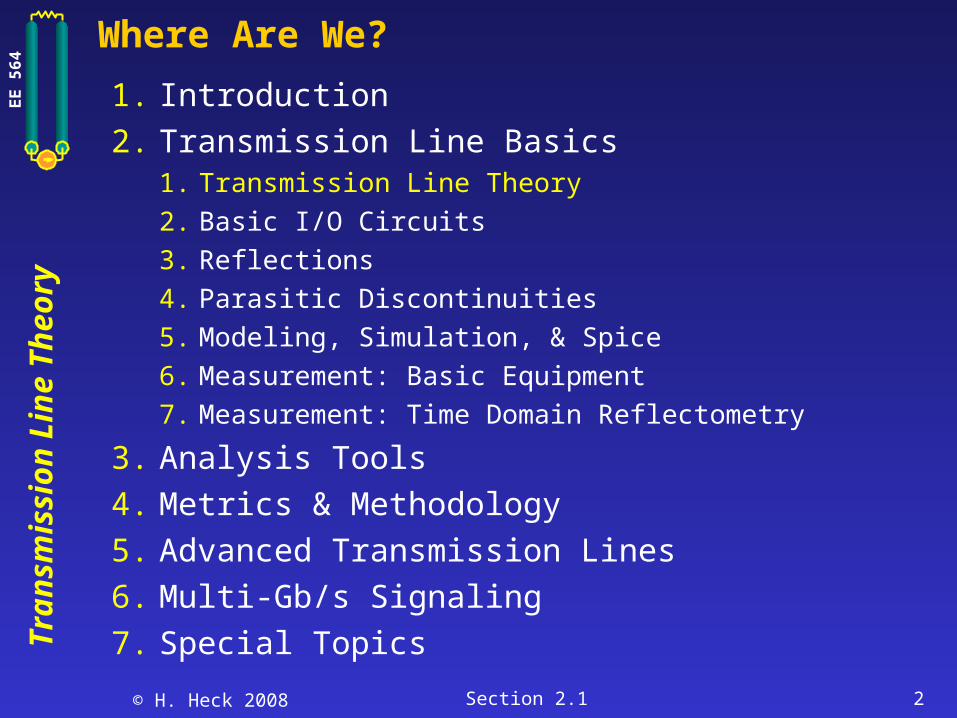
Where Are We?
1. Introduction
2. Transmission Line Basics1. Transmission Line Theory
2. Basic I/O Circuits
3. Reflections
4. Parasitic Discontinuities
5. Modeling, Simulation, & Spice
6. Measurement: Basic Equipment
7. Measurement: Time Domain Reflectometry
3. Analysis Tools
4. Metrics & Methodology
5. Advanced Transmission Lines
6. Multi-Gb/s Signaling
7. Special Topics
© H. Heck 2008 Section 2.1 3
Tra
nsm
issi
on
Lin
e T
heo
ryEE 5
64
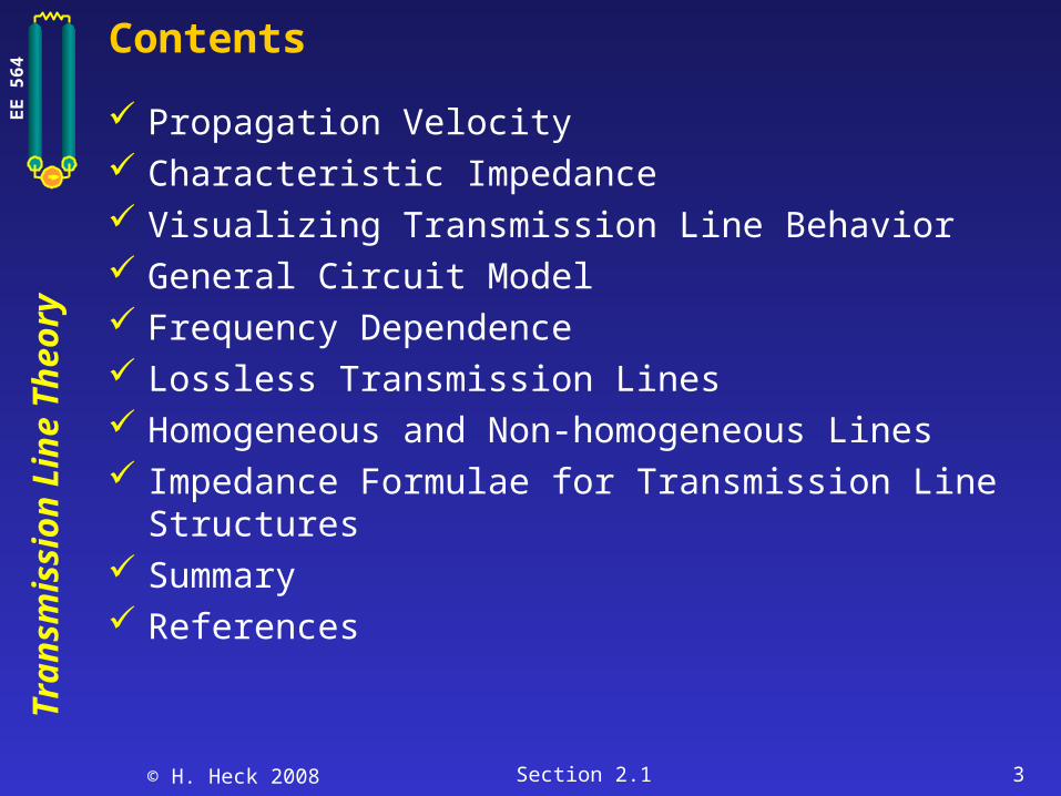
Contents
Propagation Velocity Characteristic Impedance Visualizing Transmission Line Behavior General Circuit Model Frequency Dependence Lossless Transmission Lines Homogeneous and Non-homogeneous Lines Impedance Formulae for Transmission Line Structures Summary References
© H. Heck 2008 Section 2.1 4
Tra
nsm
issi
on
Lin
e T
heo
ryEE 5
64
Propagation Velocity
Physical example:
Wave propagates in z direction
Circuit: L = [nH/cm]C = [pF/cm]
t
ILdzdz
z
V
Total voltage change across Ldz (use ): V L dI
dt
Total current change across Cdz (use ): dt
dVCI
t
VCdzdz
z
I
[2.1.1]
[2.1.2]
Simplify [2.1.1] & [2.1.2] to get the Telegraphist’s Equations [2.1.3a]
t
IL
z
V
t
VC
z
I
[2.1.3b]
I
V
Ldz
Cdz
dz
V+ dzdVdz
I+ dzdIdz
z
xy
V, I
© H. Heck 2008 Section 2.1 5
Tra
nsm
issi
on
Lin
e T
heo
ryEE 5
64
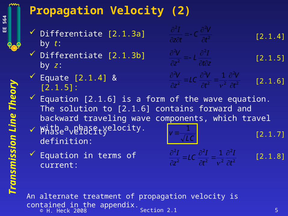
Propagation Velocity (2)
Phase velocity definition: vLC
1
[2.1.7]
Equation in terms of current:2
2
22
2
2
2 1
t
I
t
ILC
z
I
[2.1.8]
Equate [2.1.4] & [2.1.5]: [2.1.6]2
2
22
2
2
2 1
t
V
t
VLC
z
V
Differentiate [2.1.3b] by z: [2.1.5]zt
IL
z
V
2
2
2
Differentiate [2.1.3a] by t: [2.1.4]2
22
t
VC
tz
I
Equation [2.1.6] is a form of the wave equation. The solution to [2.1.6] contains forward and backward traveling wave components, which travel with a phase velocity.
An alternate treatment of propagation velocity is contained in the appendix.
© H. Heck 2008 Section 2.1 6
Tra
nsm
issi
on
Lin
e T
heo
ryEE 5
64
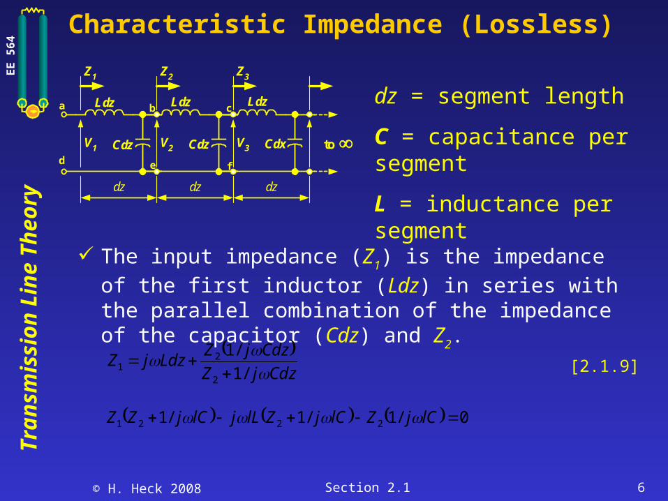
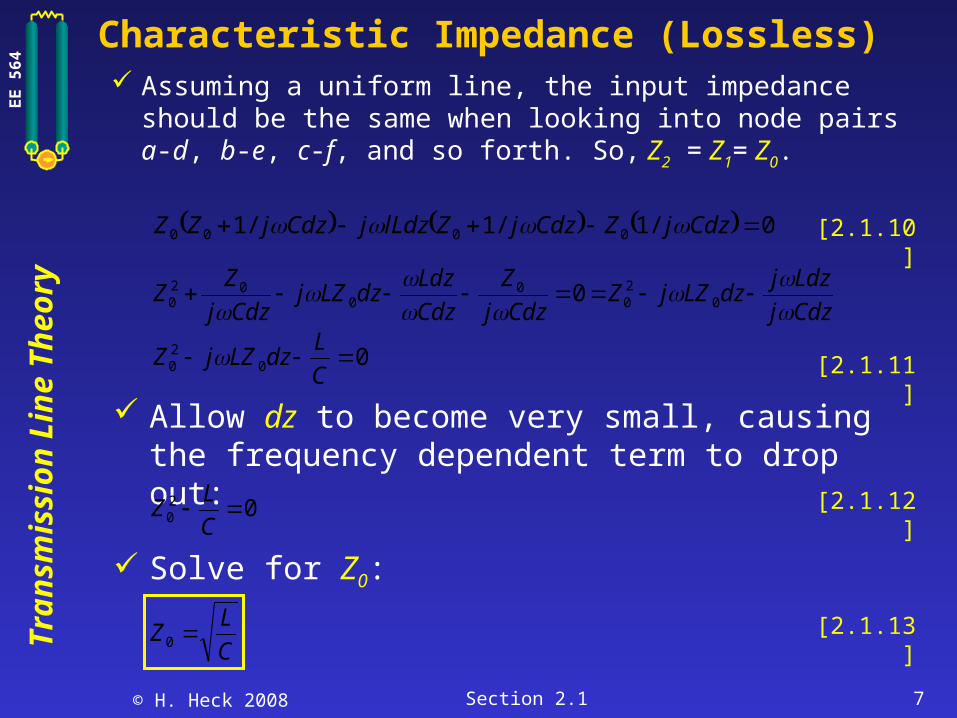
Characteristic Impedance (Lossless)
The input impedance (Z1) is the impedance of the first
inductor (Ldz) in series with the parallel combination of the impedance of the capacitor (Cdz) and Z2.
Ldz
Cdx
Z1 Z2 Z3
Ldz
Cdz
Ldz
Cdz
dz dz
V1 V3V2 to
a
fed
cb
dz
dz = segment length
C = capacitance per segment
L = inductance per segment
[2.1.9]
CdzjZ
CdzjZLdzjZ
/1
/1
2
21
0/1/1/1 2221 lCjZlCjZlLjlCjZZ
© H. Heck 2008 Section 2.1 7
Tra
nsm
issi
on
Lin
e T
heo
ryEE 5
64
Characteristic Impedance (Lossless) Assuming a uniform line, the input impedance should
be the same when looking into node pairs a-d, b-e, c-f, and so forth. So, Z2 = Z1= Z0.
0/1/1/1 0000 CdzjZCdzjZlLdzjCdzjZZ [2.1.10]
Cdzj
LdzjdzLZjZ
Cdzj
Z
Cdz
LdzdzLZj
Cdzj
ZZ
0
20
00
020 0
Allow dz to become very small, causing the frequency dependent term to drop out:
0020
C
LdzLZjZ [2.1.11]
020
C
LZ [2.1.12]
Solve for Z0:
C
LZ 0
[2.1.13]
© H. Heck 2008 Section 2.1 8
Tra
nsm
issi
on
Lin
e T
heo
ryEE 5
64
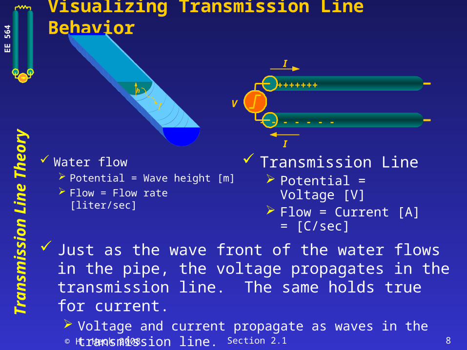
Visualizing Transmission Line Behavior
Water flow Potential = Wave height [m] Flow = Flow rate [liter/sec]
I
I
V
+++++++
- - - - - - -
Transmission Line Potential = Voltage [V] Flow = Current [A] =
[C/sec]
Just as the wave front of the water flows in the pipe, the voltage propagates in the transmission line. The same holds true for current. Voltage and current propagate as waves in the transmission line.
h
f
© H. Heck 2008 Section 2.1 9
Tra
nsm
issi
on
Lin
e T
heo
ryEE 5
64
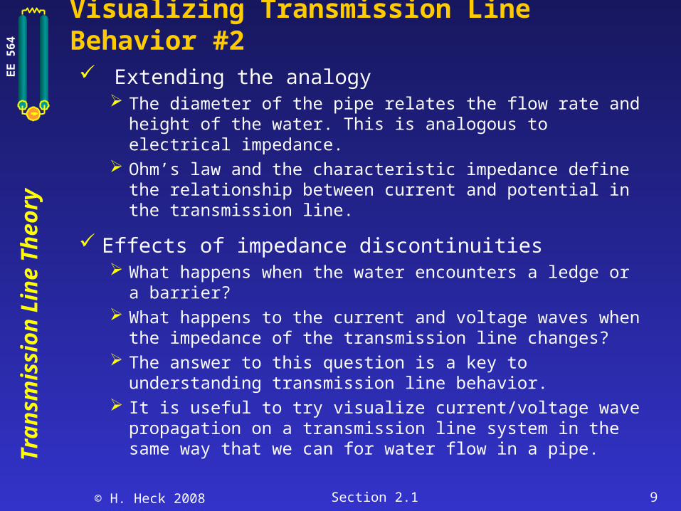
Visualizing Transmission Line Behavior #2 Extending the analogy
The diameter of the pipe relates the flow rate and height of the water. This is analogous to electrical impedance.
Ohm’s law and the characteristic impedance define the relationship between current and potential in the transmission line.
Effects of impedance discontinuities What happens when the water encounters a ledge or a
barrier? What happens to the current and voltage waves when the
impedance of the transmission line changes? The answer to this question is a key to understanding
transmission line behavior. It is useful to try visualize current/voltage wave propagation
on a transmission line system in the same way that we can for water flow in a pipe.
© H. Heck 2008 Section 2.1 10
Tra
nsm
issi
on
Lin
e T
heo
ryEE 5
64
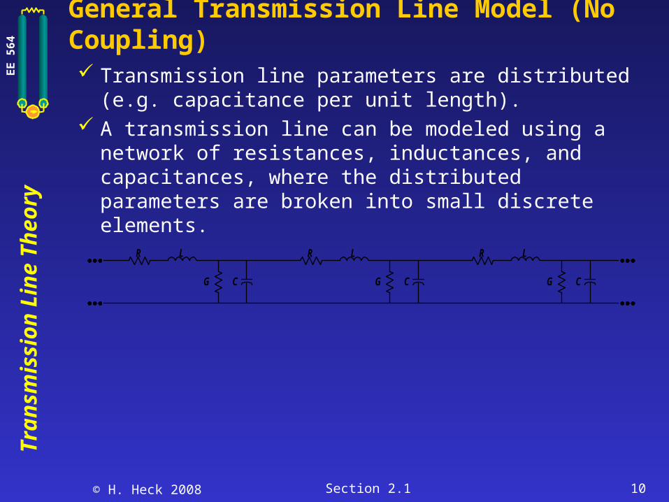
General Transmission Line Model (No Coupling) Transmission line parameters are distributed (e.g.
capacitance per unit length). A transmission line can be modeled using a network
of resistances, inductances, and capacitances, where the distributed parameters are broken into small discrete elements.
R L
G C
R L
G C
R L
G C
© H. Heck 2008 Section 2.1 11
Tra
nsm
issi
on
Lin
e T
heo
ryEE 5
64
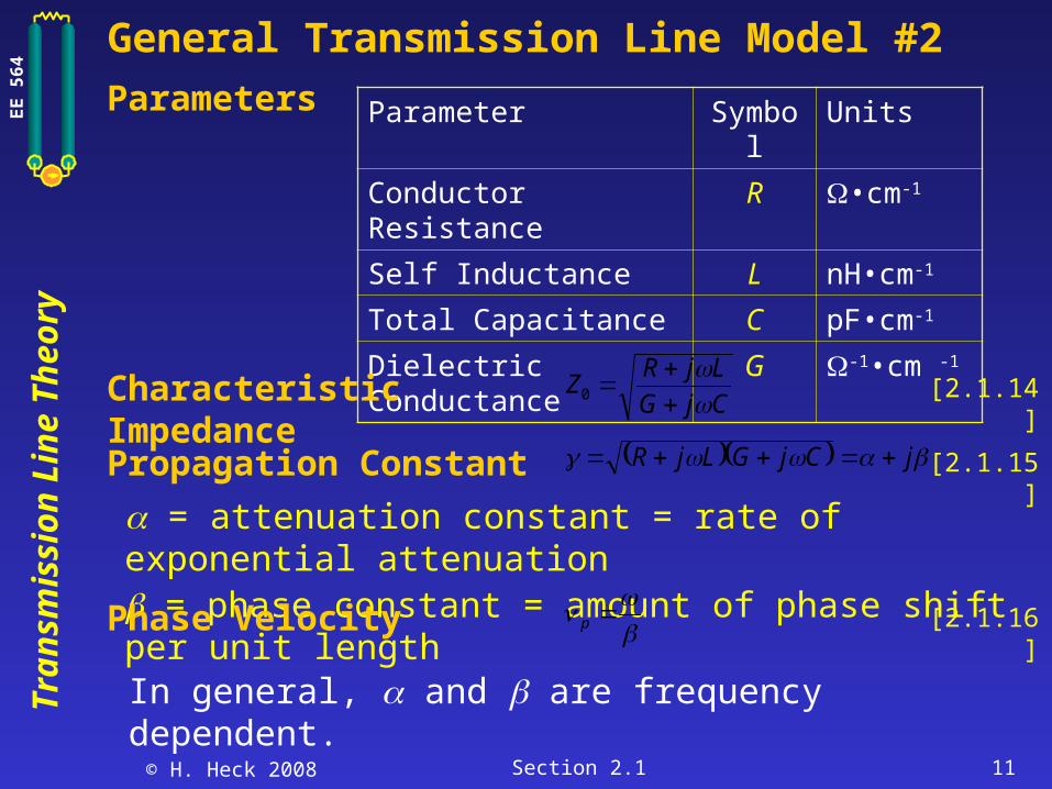
General Transmission Line Model #2
Parameter Symbol Units
Conductor Resistance R •cm-1
Self Inductance L nH•cm-1
Total Capacitance C pF•cm-1
Dielectric Conductance G -1•cm -1
Parameters
Characteristic Impedance
ZR j L
G j C0
[2.1.14]
Propagation Constant jCjGLjR [2.1.15]
= attenuation constant = rate of exponential attenuation = phase constant = amount of phase shift per unit length
pPhase Velocity [2.1.16]
In general, and are frequency dependent.
© H. Heck 2008 Section 2.1 12
Tra
nsm
issi
on
Lin
e T
heo
ryEE 5
64
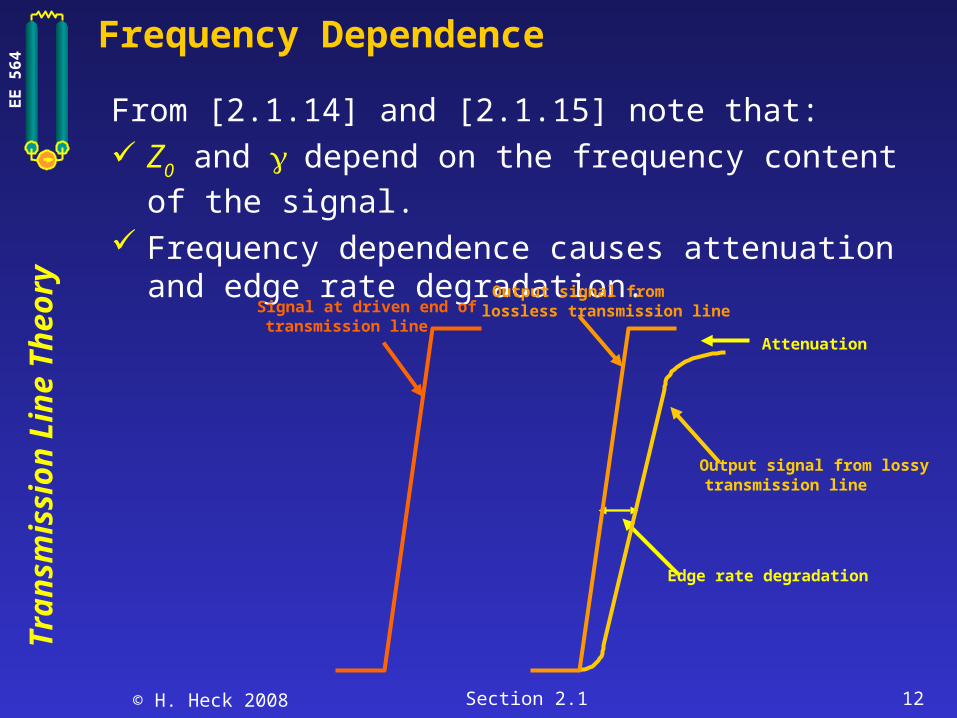
Frequency Dependence
From [2.1.14] and [2.1.15] note that: Z0 and depend on the frequency content of the
signal. Frequency dependence causes attenuation and edge
rate degradation.
Attenuation
Edge rate degradation
Output signal from lossytransmission line
Signal at driven end oftransmission line
Output signal fromlossless transmission line
© H. Heck 2008 Section 2.1 13
Tra
nsm
issi
on
Lin
e T
heo
ryEE 5
64
Frequency Dependence #2
R and G are sometimes negligible, particularly at low frequencies Simplifies to the lossless case: no attenuation & no
dispersion
In modules 2 and 3, we will concentrate on lossless transmission lines.
Modules 5 and 6 will deal with lossy lines.
© H. Heck 2008 Section 2.1 14
Tra
nsm
issi
on
Lin
e T
heo
ryEE 5
64
Lossless Transmission Lines
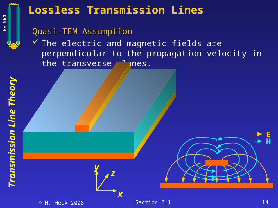
Quasi-TEM AssumptionQuasi-TEM Assumption The electric and magnetic fields are perpendicular to
the propagation velocity in the transverse planes.
x
zy
HE
© H. Heck 2008 Section 2.1 15
Tra
nsm
issi
on
Lin
e T
heo
ryEE 5
64
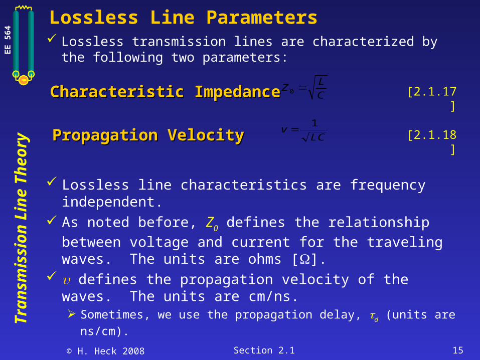
Lossless Line Parameters
Lossless line characteristics are frequency independent. As noted before, Z0 defines the relationship between
voltage and current for the traveling waves. The units are ohms [].
defines the propagation velocity of the waves. The units are cm/ns. Sometimes, we use the propagation delay, d (units are ns/cm).
C
LZ 0
vLC
1
Characteristic ImpedanceCharacteristic Impedance
Propagation VelocityPropagation Velocity
[2.1.17]
[2.1.18]
Lossless transmission lines are characterized by the following two parameters:
© H. Heck 2008 Section 2.1 16
Tra
nsm
issi
on
Lin
e T
heo
ryEE 5
64
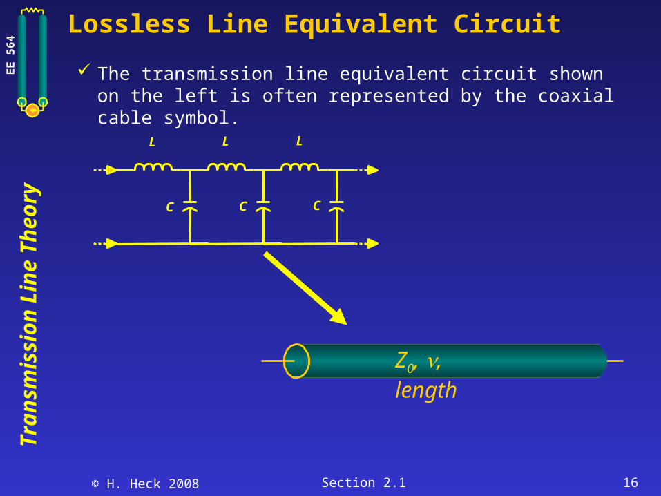
Lossless Line Equivalent Circuit
The transmission line equivalent circuit shown on the left is often represented by the coaxial cable symbol.
L
C
L
C
L
C
Z0, v, lengthZ0, , length
© H. Heck 2008 Section 2.1 17
Tra
nsm
issi
on
Lin
e T
heo
ryEE 5
64
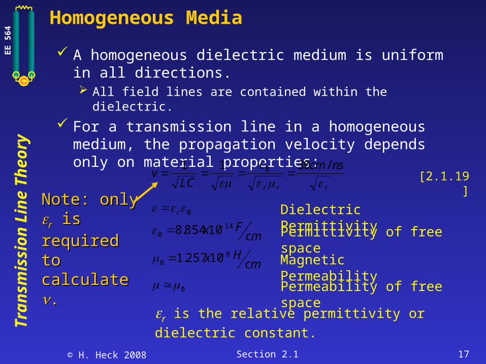
Homogeneous Media
A homogeneous dielectric medium is uniform in all directions. All field lines are contained within the dielectric.
For a transmission line in a homogeneous medium, the propagation velocity depends only on material properties:
vLC
c cm ns
r r r
1 1 300
/
[2.1.19]
0 r Dielectric Permittivity
cmFx 14
0 10854.8 Permittivity of free space
cmHx 8
0 10257.1 Magnetic Permeability
0 Permeability of free space
r is the relative permittivity or dielectric constant.
Note: only Note: only rr
is required to is required to calculate calculate ..
© H. Heck 2008 Section 2.1 18
Tra
nsm
issi
on
Lin
e T
heo
ryEE 5
64
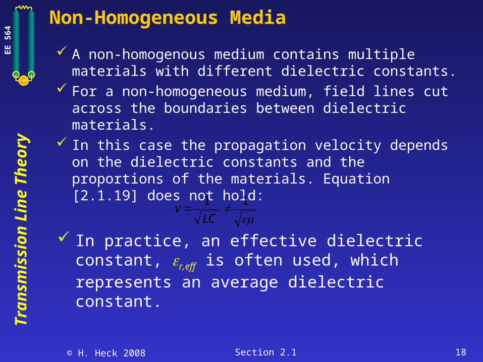
Non-Homogeneous Media
A non-homogenous medium contains multiple materials with different dielectric constants.
For a non-homogeneous medium, field lines cut across the boundaries between dielectric materials.
In this case the propagation velocity depends on the dielectric constants and the proportions of the materials. Equation [2.1.19] does not hold:
11
LC
v
In practice, an effective dielectric constant, r,eff is often used, which represents an average dielectric constant.
© H. Heck 2008 Section 2.1 19
Some Typical Transmission Line Structures
And useful formulas for Z0
© H. Heck 2008 Section 2.1 20
Tra
nsm
issi
on
Lin
e T
heo
ryEE 5
64
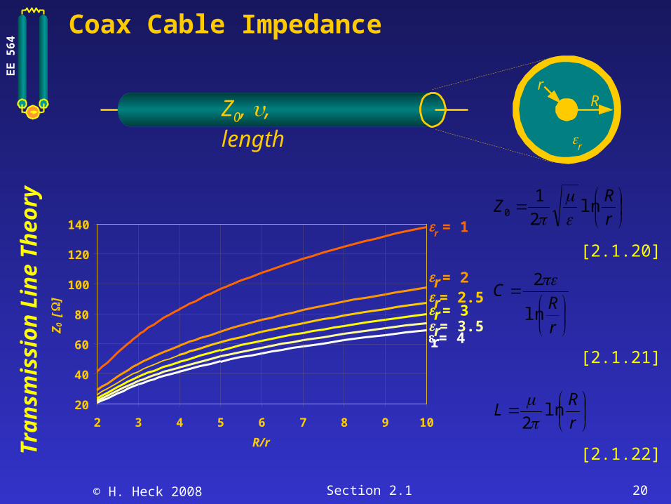
rR
r
Coax Cable Impedance
2 3 4 5 6 7 8 9 10
R/r
20
40
60
80
100
120
140
Z0 [
]
r = 1
r = 4r = 3.5r = 3r = 2.5r = 2
Z0, v, lengthZ0, , length
r
RZ ln
2
10
[2.1.20]
r
RC
ln
2
[2.1.21]
r
RL ln
2
[2.1.22]
© H. Heck 2008 Section 2.1 21
Tra
nsm
issi
on
Lin
e T
heo
ryEE 5
64
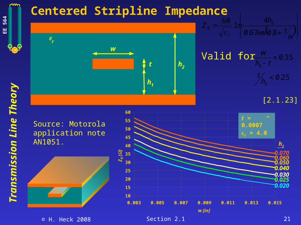
Centered Stripline Impedance
wtw
hZ
r 8.067.0
4ln
60 20
w
t
h1
h2
r
Source: Motorola application note AN1051.
35.02
th
wValid for
25.02h
t
0.003 0.005 0.007 0.009 0.011 0.013 0.015
w [in]
10
15
20
25
30
35
40
45
50
55
60
Z0
[]
0.0700.0600.0500.0400.0300.0250.020
h2
t = 0.0007”r = 4.0
[2.1.23]
© H. Heck 2008 Section 2.1 22
Tra
nsm
issi
on
Lin
e T
heo
ryEE 5
64
Dual Stripline Impedance
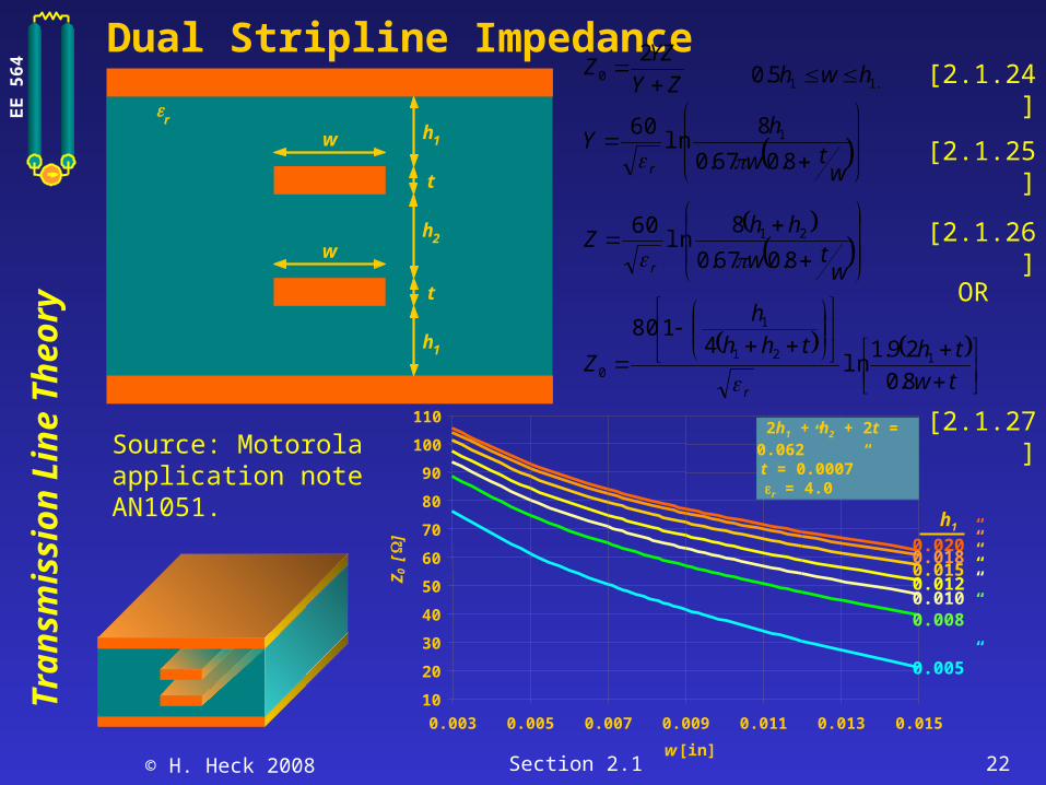
w
t
h2
h1
r
w
t
h1
ZY
YZZ
20
wtw
hY
r 8.067.0
8ln
60 1
wtw
hhZ
r 8.067.0
8ln
60 21
tw
ththh
h
Zr
8.0
29.1ln
4180
121
1
0
.115.0 hwh
Source: Motorola application note AN1051.
OR
0.003 0.005 0.007 0.009 0.011 0.013 0.015
w [in]
10
20
30
40
50
60
70
80
90
100
110Z
0 [
]
0.020”0.018”0.015”0.012”0.010”0.008”
0.005”
2h1 + h2 + 2t = 0.062” t = 0.0007”r = 4.0
h1
[2.1.24]
[2.1.27]
[2.1.25]
[2.1.26]

© H. Heck 2008 Section 2.1 23
Tra
nsm
issi
on
Lin
e T
heo
ryEE 5
64
Surface Microstrip Impedancew
t
h
r
0
d
hZ
eff
4ln
2
10
twd 67.0536.0
067.0475.0 reff
Source: National AN-991.
Source: Motorola MECL Design Handbook.
tw
hZ
r8.0
98.5ln
41.1
870
0.003 0.005 0.007 0.009 0.011 0.013 0.015
w [in]
20
40
60
80
100
120
140
160Z
0 [
]
0.025”0.020”0.015”0.012”0.009”0.006”0.004”
h
t = 0.0007”
r = 4.0
[2.1.28]
[2.1.29]
[2.1.30]
[2.1.31]
© H. Heck 2008 Section 2.1 24
Tra
nsm
issi
on
Lin
e T
heo
ryEE 5
64
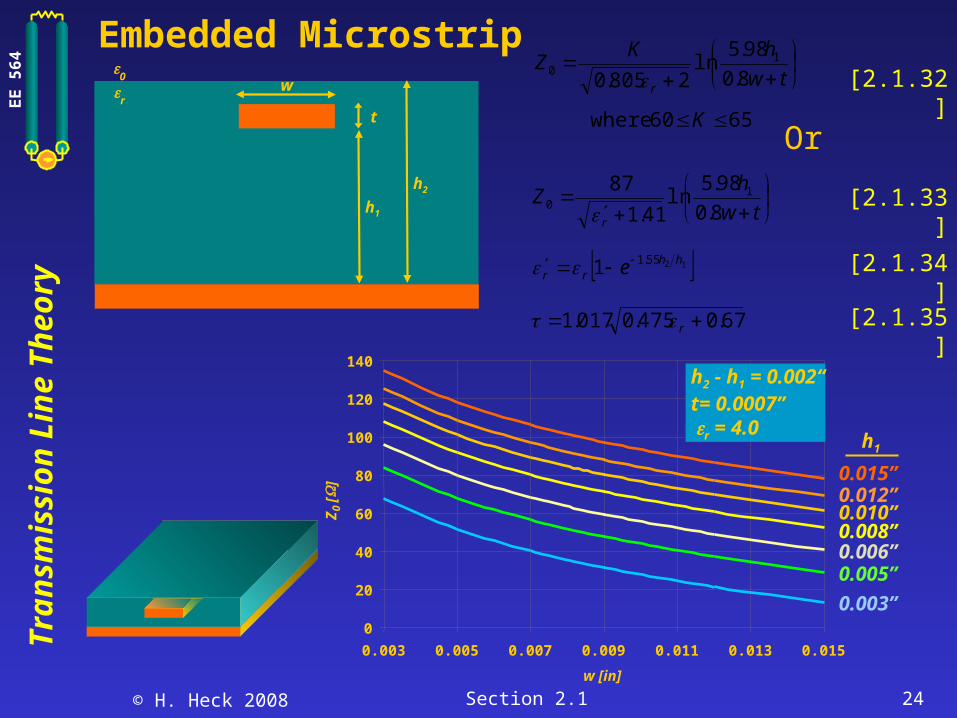
Embedded Microstrip
t
h1
r
0
w
h2
tw
hKZ
r8.0
98.5ln
2805.01
0
6560 where K
tw
hZ
r8.0
98.5ln
41.1
87 10
1255.11 hhrr e
67.0475.0017.1 r
Or
0.003 0.005 0.007 0.009 0.011 0.013 0.015
w [in]
0
20
40
60
80
100
120
140
Z0
[] 0.015”
0.012”0.010”0.008”0.006”0.005”
0.003”
h2 - h1 = 0.002“ t= 0.0007”r = 4.0
h1
[2.1.32]
[2.1.33]
[2.1.34]
[2.1.35]
© H. Heck 2008 Section 2.1 25
Tra
nsm
issi
on
Lin
e T
heo
ryEE 5
64
Summary
System level interconnects can often be treated as lossless transmission lines.
Transmission lines circuit elements are distributed. Voltage and current propagate as waves in
transmission lines. Propagation velocity and characteristic impedance
characterize the behavior of lossless transmission lines.
Coaxial cables, stripline and microstrip printed circuits are the typical transmission line structures in PCs systems.
© H. Heck 2008 Section 2.1 26
Tra
nsm
issi
on
Lin
e T
heo
ryEE 5
64
References
S. Hall, G. Hall, and J. McCall, High Speed Digital System Design, John Wiley & Sons, Inc. (Wiley Interscience), 2000, 1st edition.
H. Johnson and M. Graham, High-Speed Signal Propagation: Advanced Black Magic, Prentice Hall, 2003, 1st edition, ISBN 0-13-084408-X.
W. Dally and J. Poulton, Digital Systems Engineering, Cambridge University Press, 1998.
R.E. Matick, Transmission Lines for Digital and Communication Networks, IEEE Press, 1995.
R. Poon, Computer Circuits Electrical Design, Prentice Hall, 1st edition, 1995.
H.B.Bakoglu, Circuits, Interconnections, and Packaging for VLSI, Addison Wesley, 1990, ISBN 0-201-060080-6.
B. Young, Digital Signal Integrity, Prentice-Hall PTR, 2001, 1st edition, ISBN 0-13-028904-3.
© H. Heck 2008 Section 2.1 27
Tra
nsm
issi
on
Lin
e T
heo
ryEE 5
64
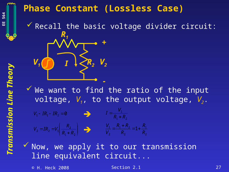
Phase Constant (Lossless Case)
Recall the basic voltage divider circuit:R1
R2V1
+
V2
-
I
We want to find the ratio of the input voltage, V1, to the output voltage, V2.
Now, we apply it to our transmission line equivalent circuit...
0211 IRIRV21
1
RR
VI
21
2122 RR
RVIRV
2
1
2
21
2
1 1R
R
R
RR
V
V
© H. Heck 2008 Section 2.1 28
Tra
nsm
issi
on
Lin
e T
heo
ryEE 5
64
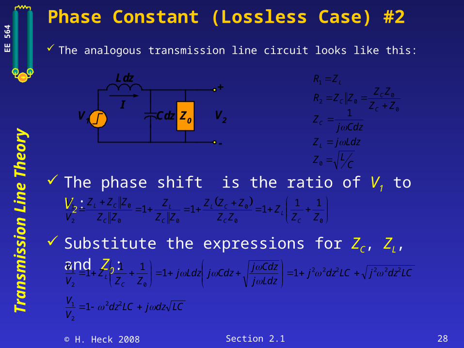
Phase Constant (Lossless Case) #2
The analogous transmission line circuit looks like this:
The phase shift is the ratio of V1 to V2:
Substitute the expressions for ZC, ZL, and Z0:
00
0
00
0
2
1 11111
ZZZ
ZZ
ZZZ
ZZ
Z
ZZ
ZZZ
V
V
CL
C
CL
C
L
C
CL
LZR 1
0
002 ZZ
ZZZZR
C
CC
CdzjZC
1
LdzjZL
CLZ 0
LCdzjLCdzjLdzj
CdzjCdzjLdzj
ZZZ
V
V
CL
222222
02
1 1111
1
LCdzjLCdzV
V 22
2
1 1
Ldz
CdzV1
+
V2
-
Z0
I
© H. Heck 2008 Section 2.1 29
Tra
nsm
issi
on
Lin
e T
heo
ryEE 5
64
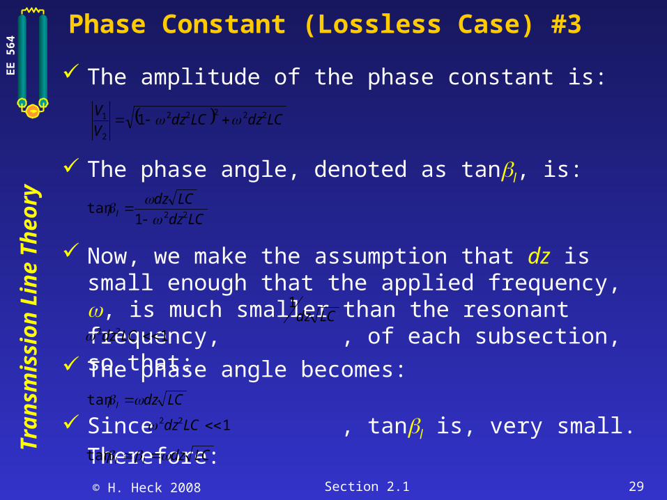
Phase Constant (Lossless Case) #3
The amplitude of the phase constant is:
The phase angle, denoted as tanl, is:
Now, we make the assumption that dz is small enough that the applied frequency, , is much smaller than the resonant frequency, , of each subsection, so that:
LCdzLCdzV
V 22222
2
1 1
LCdz
LCdzl 221
tan
LCdz1
122 LCdz
The phase angle becomes:LCdzl tan
Since , tanl is, very small. Therefore: LCdzll tan
122 LCdz
© H. Heck 2008 Section 2.1 30
Tra
nsm
issi
on
Lin
e T
heo
ryEE 5
64
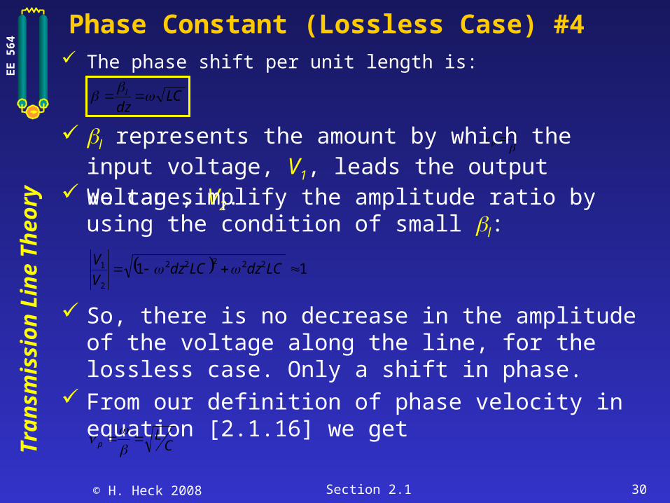
Phase Constant (Lossless Case) #4 The phase shift per unit length is:
p l represents the amount by which the input voltage, V1,
leads the output voltage, V2. We can simplify the amplitude ratio by using the
condition of small l:
So, there is no decrease in the amplitude of the voltage along the line, for the lossless case. Only a shift in phase.
From our definition of phase velocity in equation [2.1.16] we get
LCdz
l
11 22222
2
1 LCdzLCdzV
V
CL
p